Download Get - Wiley Online Library

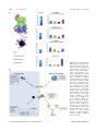
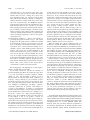
Proteomics 2011, 11, 1153–1159
1153
DOI 10.1002/pmic.201000548
TECHNICAL BRIEF
Mass spectrometry-based immuno-precipitation
proteomics – The user’s guide
Sara ten Have, Se´verine Boulon, Yasmeen Ahmad and Angus I. Lamond
Wellcome Trust Centre for Gene Regulation and Expression, College of Life Sciences, University of Dundee,
Dundee, Scotland, UK
Immuno-precipitation (IP) experiments using MS provide a sensitive and accurate way of
characterising protein complexes and their response to regulatory mechanisms. Differences in
stoichiometry can be determined as well as the reliable identification of specific binding partners. The quality control of IP and protein interaction studies has its basis in the biology that is
being observed. Is that unusual protein identification a genuine novelty, or an experimental
irregularity? Antibodies and the solid matrices used in these techniques isolate not only the
target protein and its specific interaction partners but also many non-specific ‘contaminants’
requiring a structured analysis strategy. These methodological developments and the speed and
accuracy of MS machines, which has been increasing consistently in the last 5 years, have
expanded the number of proteins identified and complexity of analysis. The European Science
Foundation’s Frontiers in Functional Genomics programme ‘Quality Control in Proteomics’
Workshop provided a forum for disseminating knowledge and experience on this subject. Our
aim in this technical brief is to outline clearly, for the scientists wanting to carry out this kind of
experiment, and recommend what, in our experience, are the best potential ways to design an
IP experiment, to help identify possible pitfalls, discuss important controls and outline how to
manage and analyse the large amount of data generated. Detailed experimental methodologies
have been referenced but not described in the form of protocols.
Received: August 31, 2010
Revised: December 7, 2010
Accepted: December 10, 2010
Keywords:
Cell biology / Cumulative analysis / Immuno-precipitation / Protein frequency /
Quality control / SILAC
The ability to purify and specifically produce antibodies in
the late 1960s and 1970s [1–3] facilitated the development of
targeted protein analysis. Antibodies facilitated protein
Western blotting [4]. Protein interaction studies began
analysing one protein at a time. Today the use of MS
[5, 6] in combination with immuno-precipitation (IP) [7]
allows hundreds of proteins to be identified in a single
experiment. However, usually the majority of proteins identified in IP experiments are non-specific binders [6]. The solid
Correspondence: Dr. Sara ten Have, Wellcome Trust Centre for
Gene Regulation and Expression, College of Life Sciences,
University of Dundee, Dow Street, Dundee DD1 5EH, Scotland,
UK
E-mail: [email protected]
Fax: 144-1382-348072
Abbreviations: IP, immuno-precipitation; PFL, Protein Frequency
Library
& 2011 WILEY-VCH Verlag GmbH & Co. KGaA, Weinheim
matrices, e.g. agarose, sepharose and magnetic beads, which
are essential to the IP protocol, are the main contributors to
non-specific binding, with a smaller contribution from
protein binding to antibodies and tags (Fig. 1A).
SILAC [8] has ushered in a more accurate, multiplexed
method of condition-dependent comparison, which has in
turn enabled the relative quantitation of putative protein
interactors and contaminants in IP experiments [5–6].
SILAC labelling utilises artificially increased levels (98% in
specific amino acids – generally arginine and lysine) of
stable isotopes (i.e. carbon 13, nitrogen 15 and deuterium).
Cells of choice can be grown in normal ‘light’ cell culture
media (arginine 0, lysine 0), or combinations of arginine
(13C6, ‘R6’ or 13C6, 15N4, ‘R10’) and lysine (4, 4, 5, 5-D4,
‘K4’, 13C6, ‘K6’ or 13C6, 15N2, ‘K8’) supplemented media.
Aside from the convenience of combining the bead control
(arginine 0, lysine 0), with the IP of interest (arginine 6,
lysine 4), and if required a third condition (e.g. comparing
www.proteomics-journal.com
1154
S. ten Have et al.
Proteomics 2011, 11, 1153–1159
Figure 1. (A) The above diagram
characterises the relative changes (percentage of protein identified in IP results (right) and
total percentage of protein as a
fraction of cell extract (left)) in
terms of the abundance of the
proteins identified in response
to different experimental procedures.
Whether
comparing
intensities directly in a label-free
experiment, or utilising a SILAC
approach to quantify proteins,
these changes should be taken
into consideration. It also indicates the importance of having
a bead control (non-specific
proteins which bind to beads)
characterised for every experiment – because the non-specific
proteins identified in bead
controls vary for different cell
lines, antibodies, beads, etc.
(B) The immuno-precipitation
workflow. Protein–protein interactions analysis utilising IP
techniques can be approached
in many different ways, using
complex samples such as tissue
biopsies, or single cell-type
samples, and with labelled or
label-free scenarios, illustrated
by the flow chart.
& 2011 WILEY-VCH Verlag GmbH & Co. KGaA, Weinheim
www.proteomics-journal.com
Proteomics 2011, 11, 1153–1159
interaction partners of wild type and mutant proteins,
arginine 10, lysine 8), this protocol can reduce or eliminate
both machine variation and human error.
The IP preparations from each sample are mixed in equal
ratios (1:1:1); therefore, proteins that do not change between
conditions (experimental contaminants) will have an expected
log 2 ratio of 0 (in practice 0.32olog 2 ratioo0.26, which is
not symmetrical, but characterised experimentally). Proteins
that have been enriched relative to the control (putative
specific interaction partners) will have increased log 2 ratios
(i.e. usually 40.26) and environmental contaminants generally have a low log 2 ratio (typically o 0.32, see Fig. 3).
Protocols and information regarding these SILAC methodologies are available at www.LamondLab.com.
Experimental design is dependent on the question being
asked (Fig. 1B), and therefore dictates control(s) required to
accurately distinguish changes due to biologically relevant
effects. An initial, exploratory IP experiment is usually
1155
recommended. Tricks for the optimisation of IP experimental design are given in Table 1 to help increase the
efficiency of the protein recovery and to reduce and/or
identify putative contaminants.
One important step to improve the accuracy of conclusions drawn from IP data is to characterise the range of nonspecific binding proteins. The non-specific proteins identified in IP experiments vary considerably and depend on
parameters such as cellular fraction utilised, cell type, bead
type, etc. This was described previously in ‘Identifying
specific protein interaction partners using quantitative MS
and bead proteomes’ [6], and has since been developed into a
more general approach in the form of the Protein Frequency
Library (PFL) [5] and described below (see Data management section).
To look at and assess the statistics of the entire population of identified proteins is required for labelled and unlabelled scenarios alike (Figs. 2 and 3). The way to go about
Figure 2. The graph depicts the normalised distribution of average (log) protein intensities detected in all protein identifications, showing
the normalised distribution of the population. The three graphs derived from the main graph describe the frequency of occurrence of the
proteins in each protein intensity region. It is interesting to note that the number of proteins in the highest intensity range is 100-fold less
than the numbers seen in the low and mid-intensity ranges. This indicates that the very high intensity proteins are only a small percentage
of the proteins seen. Secondly, the graphs show a positive correlation between protein intensity and frequency of occurrence, which
suggests that high-intensity proteins have a higher likelihood of being contaminants. Therefore, using a tool such as the Protein
Frequency Library to tease apart significance of these protein identifications is helpful. The data shown above consists of 21 682 independent protein identifications, from 140 IP experiments performed in two different laboratories. These IP experiments included GFPtagged protein pull downs, endogenous protein pull downs and included the use of agarose, sepharose and dynabeads. The peak of 600
proteins at 0 is due to the ability of MaxQuant to identify proteins/peptides from the MS/MS spectra, with insufficient information from the
MS spectra to determine intensities.
& 2011 WILEY-VCH Verlag GmbH & Co. KGaA, Weinheim
www.proteomics-journal.com
1156
S. ten Have et al.
this is described below in two sections – firstly for (a) labelfree IPs and secondly for (b) labelled IP experiments:
(a) Unlabelled IP analysis
(i) Population statistics – This requires the frequency of
protein intensities to be measured (note raw ion
intensities should not be compared directly, but the
median of the intensities from all peptides identified for
a protein, with any skewing due to experimental and/or
machine error/inaccuracy factored into these data).
Examine the range of these values (using the log of the
intensity values as this is more practical to deal with) and
logically divide these evenly into bins. Then group
proteins by their corresponding bins. This gives the
frequency of the average intensity values of the identified
proteins (Fig. 2). This is useful for two main reasons. It
provides a measure of the quality of the data (i.e. it
should show a normal or bell-shaped curve, if not the
data are biased or skewed) and highlights which proteins
Proteomics 2011, 11, 1153–1159
are significantly enriched – and therefore putative,
specific interactor(s) for the bait protein.
(ii) Determining significance – In Fig. 2, the graph was
generated from 140 separate IP experiments – consisting of 21 682 protein identifications, using human
cell lines, many different antibodies, bead types
and GFP tagged proteins from multiple researchers
in two different laboratories, using Thermo Orbitrap
XL and Velos mass spectrometers. The analysis of
ion intensities, as an example of label-free experimental design, generated a log of peak intensity
population centred over 6.75. This value may vary
for different mass spectrometers and/or experimental
set ups. Be aware it is dependent on the accuracy
and level of detection possible in the mass spectrometer but the graph should still have a bell-shaped
distribution.
With label-free analysis, the margins of siginificance
are less clear than with the SILAC (or other labelling
Figure 3. An example of protein ratio frequency graph showing the normalised distribution and the median value of the data. The
‘normalised bell-shaped curve’ is centred over a log ratio of 0; this means the mixing of SILAC samples was done accurately (i.e. exactly
equal protein levels from each extract mixed). If the ratios deviate significantly from this, then likely an error was made when mixing, and
ratio values will need to be adjusted accordingly (see Determining significance section). The green and red vertical lines indicate the
(arbitrary) borders of significance. In general, proteins with high SILAC ratios usually correspond to specific interaction partners.
Ambiguity appears largely in the pink zone, where proteins have log ratios close to 0 and can correspond either to contaminants, or to
specific interaction partners with low affinity and/or low abundance. To discriminate, the PFL can be helpful.
& 2011 WILEY-VCH Verlag GmbH & Co. KGaA, Weinheim
www.proteomics-journal.com
Proteomics 2011, 11, 1153–1159
1157
Table 1. Pitfalls of immuno-precipitation methodology
Antibody specificity
Do you know how specific your antibody is for binding to your target protein? Do not rely on specificity of commercial
antibodies without checking this! It may be the case that it is targeted to a motif of your protein that has high homology in other
proteins that have a similar function. Check this possibility by blasting your protein (http://blast.ncbi.nlm.nih.gov/Blast.cgi). Do
some of the proteins identified in your experiment match these homologous proteins? If so, the significance of the assumed
interaction must be confirmed.
Antibody affinity
There is the possibility that the binding of an antibody to its target is weak, or that there is competition within the sample for the
binding sites. This can be checked by analysing the sample flow-through. Additionally, using a different solid matrix, e.g.
agarose, sepharose or magnetic beads as an alternative could be considered. Antibody specificity and affinity should be
checked and the IP protocol optimised prior to MS analysis.
Pre-clearing
Many commercial IP methods specify ‘pre-clearing’ of cell extracts with sepharose G-beads. This does reduce levels of nonspecific binding proteins, but it may also be the case that the genuine target protein has a high affinity for the matrix, or is of low
abundance and lost during the ‘pre-clearing’ step. Avoid this by analysing the eluate of the pre-clearing beads – you never know
what you might find! Also, keep incubation times short to limit the loss of weak interactions partners.
Affinity tags
Be aware that protein (e.g. GST) tags can also bind certain non-specific proteins in the extract. Additionally, they may cause
steric hindrance that masks the binding site of an important interactor. Counter this problem by the location of the tag, i.e. C
and N terminal.
Bead controls
Always characterise non-specific binding possibilities. Run all control samples exactly the same way as for the analysis of
interest, with a control antibody, or with beads only, and compare which proteins are identified. In the case of SILAC, this is
included in the final sample run for analysis; in label-free scenarios this needs to be run in parallel to the IP. This can be treated
as your Bead Control. By compiling data from separate experiments, a global bead proteome can be compiled. To verify the
legitimacy of either a contaminant or a putative interactor, check proteins against the Protein Frequency Library.
(www.proteinfrequencylibrary.com).
Statistical analysis
It is crucial to remember that an IP enriches a specific group of proteins. To normalise the data the contaminating proteins
which are inherent with IPs can be used (see Figs. 2 and 3).
Washing stringency
Washing steps, which are common in all IP protocols, are a major determining factor of the final protein identifications (Fig. 1).
Having a high number of washing steps (43) with high salt concentration (4150 mM salt component) will increase the risk of
losing weak interacting proteins and also increase the chance of disassembling protein complexes. The best way to perform IPs
to increase detection of weakly interacting proteins is to use short incubation times (30 min to 1 h), preferably at 41C, and with
minimal low salt washing.
Sample complexity
Due to many of the above-described pitfalls IPs are, despite being an enriched sample, still inherently complex. To eliminate
co-elution of peptides and the statistical and quantitative issues that may arise from this, performing pre-fractionation of your
samples is practical. This can be done, for example, with size exclusion and/or reverse-phase chromatography, as well as by ingel digestion or IEF fractionation techniques.
strategy) ratios. This is due to the SILAC ratios of
high abundance, non-specific binding proteins being
unchanged (i.e. having a ratio of 1) whereas with labelfree experiments the proteins with log intensities 47.25
will comprise both specific, enriched proteins and
abundant contaminant proteins. The remaining proteins
in the lower intensity ranges (o7.25) may contain both
contaminants and lower abundance specific interaction
proteins. In the case of label-free experiments, it is
therefore important to have a well-characterised bead
control for your experiment, to help identify likely
contaminant proteins. Quantification generally requires
at least three technical and biological replicates of the
& 2011 WILEY-VCH Verlag GmbH & Co. KGaA, Weinheim
control IP, specific IP and bead control, with identical
protein loading, MS and HPLC conditions.
(b) Labelled IP analysis (SILAC, iTRAQ, etc.)
(i) Population statistics – It should be noted that although a
level of significance can be determined, proteins with
label ratios values below this significance level may still
be specific and of interest (Fig. 3). The normalised curve
should, in a labelled context, be centred over a log ratio
value of zero (assuming mixing of labelled samples was
1:1), because the majority of proteins (which are nonspecific binding proteins or contaminants) in the
samples should be unchanged and therefore have
www.proteomics-journal.com
1158
S. ten Have et al.
equivalent ratios. In cases where the centre of the curve
is located over log ratio of 0.08, for example, this visually
indicates there has been a mixing error, where more
heavy labelled proteins were mixed in with the light
label, and all ratios should be adjusted accordingly (i.e.
all ratios should be recalculated with the increase of log
ratio 0.08 compensated for). The MaxQuant output is
in.txt file format and generates ratio information in H/L,
H/M and M/L (which are also reversible to necessitate
label swapping experiments), and also intensity information for label-free analysis, allowing convenient manipulation via either custom software or Microsoft Excel and
comprises detailed SILAC information, peptide identification and statistical significance values on the peptide
and protein levels.
(ii) Determining significance – This is done initially by
generating the graph described in Fig. 3. The cut-off
designated on the graph shown is arbitrary and should
be decided by the scientist. It is important to note that
there are inevitably some limitations in this experimental method, due to non-stoichiometric binding of, low
abundance and/or weakly binding genuine interaction
partners. This means the proteins identified in the
region coloured pink in Fig. 3 may nonetheless contain
some specific proteins of interest. Within the current
scope of one single experiment, this significance cannot
be determined unambiguously. Therefore, the use of the
PFL, with its cumulative statistical strength, based on
large numbers (hundreds) of IP experiments can help to
predict which of the proteins in this region will be
contaminants or putative interaction partners.
Data management – The following two sections apply to
label-free and labelled scenarios alike.
As previously mentioned, typically the numbers of
proteins identified using MS in IP experiments range from
70 to 600, depending on washing conditions, antibody
affinity, etc. (Fig. 1A). Generating a dynamic record of
which proteins are detected under which conditions (e.g.
bead type, cell type, antibody, etc.) is a beneficial, accurate
and in the long term, time saving exercise. This has been
done using data management systems derived from Business Intelligence methodologies, providing a dynamic,
continually updated list of proteins, with statistics of
occurrence and significance in relation to experimental
metadata. The PFL [5] helps to evaluate objectively whether a
protein identified is a genuine interactor or is likely to be a
non-specific binder (see http://www.proteinfrequency
library.com/). The magnitude of data now being produced
in MS analyses is not, in our opinion, a reason for
employing purification techniques with greater stringency,
which risks losing important specific interaction partners.
The technologies have increased in speed and accuracy with
the rationale of allowing more peptides to be identified and
quantified in each experiment/run. Therefore, utilising all
of these data is a more economical and sensible application
& 2011 WILEY-VCH Verlag GmbH & Co. KGaA, Weinheim
Proteomics 2011, 11, 1153–1159
of time and resources. The benefits of such data ‘conservation’ have been seen with initiatives such as the Cochrane
Reviews [9], in the medical trial field, which used only
randomised, controlled medical trials. This meant the data
going into the analyses was of higher quality (randomised
controlled trials are a better sampling method for seeing the
true effects of medical interventions) and therefore significance, and the outcomes of a number of trials were collectively analysed, yielding stronger statistics and more
accurate conclusions. This is a similar strategy to the one
employed in the Lamond Laboratory (www.lamondlab.com)
and the Wellcome Trust Centre for Gene Regulation and
Expression (http://gre.lifesci.dundee.ac.uk/index.html) with
proteomic approaches. We are curating all of the metadata;
results and machine variables to better understand, scrutinise and critically appraise our data, with an aim to apply the
results rapidly to biology and medicine, and to generate
publicly available resources such as the PFL.
When presenting these data in publication form, one
should also consider the Minimum Information About a
Proteomics Experiment (MIAPE) [10] and Minimum Information about a Molecular Interaction Experiment (MIMIx)
[11] guidelines for what to include. Also depositing Proteomics results in databases such as PRIDE (http://www.ebi.ac.uk/pride/) [12], and interaction data into an IMEx
Consortium database such as IntAct [13] allows for cumulative data analysis and easy access by reviewers for your data.
Pathway analysis – The log ratios or log intensity values
alone of proteins which could potentially be interactors (i.e. in
the pink region of Fig. 2) do not justify their identification as
interaction partners. Their biological functions, and therefore
previously known interactions, can moreover provide additional confidence to justify their inclusion. In addition to coIP experiments to verify specific interactors, in silico analysis
can be done by individually searching the proteins and
assessing the literature for their known associations, or else
several software packages are available with which you can do
this. It is also helpful to perform follow-up experiments
using, for example, Western blot analysis and immunofluorescence studies, to provide additional independent
evidence to support the protein interactions identified using
MS. String analysis software (http://string-db.org/ [14]) is
freely available and the protein associations are selectable, i.e.
you can specify experimental associations, etc. A more
expensive option, but more extensive software, is the Ingenuity Pathway Analysis package (www.ingenuity.com).
The authors thank Doulas Lamont and Kenneth Beattie at the
University of Dundee’s Fingerprints Proteomics facility for technical
support, Matthias Mann and his Laboratory for data contribution.
This work was supported in part by Wellcome Trust Program Grant
073980/Z/03/Z (to A.I. L.) with additional support from
European Union (EU) FP7 Grant Proteomics Specification in
Time and Space (PROSPECTS), EU Network of Excellence Grant
European Alternative Splicing Network (EURASNET) and an
www.proteomics-journal.com
Proteomics 2011, 11, 1153–1159
interdisciplinary Radical Solutions for Researching the Proteome
(RASOR) initiative, which is supported by the Biotechnology and
Biological Sciences Research Council (BBSRC), Engineering and
Physical Sciences Research Council, Scottish Higher Education
Funding Council and Medical Research Council (MRC).
The authors have declared no conflict of interest.
References
[1] Gally, J. A., Edelman, G. M., Protein–protien interactions
among L polypeptide chains of Bence-Jones proteins
and human gamma-globulins. J. Exp. Med. 1964, 119,
817–836.
[2] Heidelberger, M., Kendall, F. E., A quantitative study of the
precipitin reaction between type III Pneumococcus polysaccharide and purified homologous antibody. J. Exp. Med.
1929, 50, 809–823.
[3] Kohler, G., Milstein, C., Continuous cultures of fused cells
secreting antibody of predefined specificity. Nature 1975,
256, 495–497.
[4] Burnette, W., ‘‘Western blotting’’: electrophoretic transfer of
proteins from sodium dodecyl sulfate–polyacrylamide gels
to unmodified nitrocellulose and radiographic detection
with antibody and radioiodinated protein A. Anal. Biochem.
1981, 112, 195–203.
[5] Boulon, S., Ahmad, Y., Trinkle-Mulcahy, L., Verheggen, C.
et al., Establishment of a Protein Frequency Library and
its application in the reliable identification of specific
protein interaction partners. Mol. Cell. Proteomics 2010, 9,
861–879.
& 2011 WILEY-VCH Verlag GmbH & Co. KGaA, Weinheim
1159
[6] Trinkle-Mulcahy, L., Boulon, S., Lam, Y. W., Urcia, R. et al.,
Identifying specific protein interaction partners using
quantitative mass spectrometry and bead proteomes. J. Cell
Biol. 2008, 183, 223–239.
[7] Bonifacino, J. S., Dell’Angelica, E. C., Springer, T. A.,
Current Protocols in Immunology, Wiley, New York 2001,
pp. 8.3.1–8.3.28.
[8] Ong, S.-E., Blagoev, B., Kratchmarova, I., Kristensen, D. B.
et al., Stable isotope labeling by amino acids in cell culture,
SILAC, as a simple and accurate approach to expression
proteomics. Mol. Cell. Proteomics 2002, 1, 376–386.
[9] Levin, A., The Cochrane Collaboration. Ann. Intern. Med.
2001, 135, 309–312.
[10] Taylor, C. F., Paton, N. W., Lilley, K. S., Binz, P.-A. et al., The
minimum information about a proteomics experiment
(MIAPE). Nat. Biotech. 2007, 25, 887–893.
[11] Orchard, S., Salwinski, L., Kerrien, S., Montecchi-Palazzi, L.
et al., The minimum information required for reporting a
molecular interaction experiment (MIMIx). Nat. Biotech.
2007, 25, 887–893.
[12] Vizcaı´no, J. A., Coˆte´, R., Reisinger, F., Foster, J. M. et al.,
A guide to the Proteomics Identifications Database proteomics data repository. Proteomics 2009, 9, 4276–4283.
[13] Aranda, B., Achuthan, P., Alam-Faruque, Y., Armean, I.
et al., The IntAct molecular interaction database in 2010.
Nucleic Acids Res. 2010, 38, 525–531.
[14] Jensen, L. J., Kuhn, M., Stark, M., Chaffron, S. et al.,
STRING 8 – a global view on proteins and their functional
interactions in 630 organisms. Nucleic Acids Res. 2009, 37,
D412–D416.
www.proteomics-journal.com