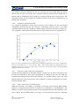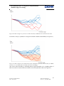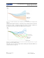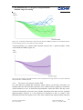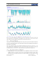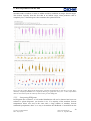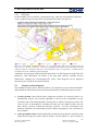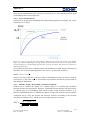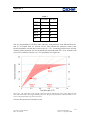
1
User guide to ECMWF forecast
products
© Copyright 2011, 2013 ECMWF
Location: Livelink 4320059
Date: 23/07/2013
Owner: Erik Andersson
Version 1.1
Date of original issue:
Author:
Version number
1.1
October 2011
Anders Persson
Date
23/07/2013
Changed by
Erik Andersson
Change description
New terminology, ENS
initial perturbations
2
Location: Livelink 4320059
Date: 23/07/2013
Owner: Erik Andersson
Version 1.1, Page 2 of 129
1.
Introduction.............................................................................................................................. 1
2.
The ECMWF forecasting and assimilation system ............................................................... 2
2.1.
2.1.1.
The model equations..................................................................................... 2
2.1.2.
The numerical formulation .......................................................................... 2
2.1.3.
The rationale for high resolution ................................................................. 3
2.1.4.
Topographical and climatological fields ...................................................... 3
2.1.5.
The formulation of physical processes ......................................................... 4
2.1.6.
The land surface model ................................................................................ 6
2.1.7.
The ocean wave model.................................................................................. 6
2.2.
The dynamic ocean model .............................................................................................. 7
2.3.
Data assimilation ............................................................................................................. 7
2.3.1.
The four-dimensional data assimilation (4D-Var) ....................................... 8
2.3.2.
The ECMWF early delivery system ............................................................. 8
2.4.
3.
The ECMWF global atmospheric model ....................................................................... 2
Retrieving ECMWF forecasts ......................................................................................10
2.4.1.
Temporal retrieval ..................................................................................... 10
2.4.2.
Spatial retrieval .......................................................................................... 10
2.4.3.
Orography .................................................................................................. 10
2.4.4.
The bi-linear interpolation ......................................................................... 10
2.4.5.
The subsampling procedure ....................................................................... 12
2.4.6.
Interpolating land and sea points............................................................... 13
2.5.
The relation between grid point values and observations...........................................15
2.6.
Some characteristics of NWP output ...........................................................................16
2.6.1.
Forecast error growth ................................................................................ 16
2.6.2.
Downstream spread of influence ................................................................ 16
2.6.3.
The relation between scale and predictive skill ......................................... 17
2.6.4.
Forecast “jumpiness” ................................................................................. 20
2.6.5.
Flip-flopping forecasts ................................................................................ 21
2.6.6.
Jumpiness and forecast skill....................................................................... 22
2.6.7.
Forecast trends cannot be extrapolated ..................................................... 22
2.6.8.
Other state-of-the-art deterministic models .............................................. 22
The forecast ensemble ...........................................................................................................25
3.1.
The rationale behind the ensemble...............................................................................25
3.1.1.
Qualitative use of the ensemble .................................................................. 25
3.1.2.
Quantitative use of the ENS ....................................................................... 25
3.1.3.
Characteristics of a good ensemble ............................................................ 26
3.2.
Generation of the ENS ..................................................................................................26
i
Location: Livelink 4320059
Date: 23/07/2013
Owner: Erik Andersson
Version 1.1, Page i of 129
3.2.1.
Different perturbation techniques ............................................................. 26
3.2.2.
Quality of the individual perturbed analyses ............................................ 29
3.2.3.
Quality of the individual perturbed forecasts............................................ 31
3.3.
3.3.1.
The 10-day range ........................................................................................ 32
3.3.2.
The day 9 to 10 overlap .............................................................................. 33
3.3.3.
The 10 to 15 day range ............................................................................... 33
3.3.4.
Forecasts from 15 to 32 days ...................................................................... 33
3.3.5.
Seasonal forecast ........................................................................................ 33
3.4.
4.
The ensemble at different lead times ...........................................................................32
Basic forecast products .................................................................................................33
3.4.1.
“Postage stamp maps”................................................................................ 33
3.4.2.
“Spaghetti diagrams” ................................................................................. 34
3.4.3.
“Plumes” ..................................................................................................... 34
3.4.4.
Ensemble mean and median....................................................................... 35
3.4.5.
Ensemble spread......................................................................................... 35
3.4.6.
Probabilities ................................................................................................ 36
3.4.7.
Forecast expressed in terms of intervals .................................................... 36
Recommendations on categorical and probabilistic medium-range forecasting ...............37
4.1.
Relation between deterministic and probabilistic forecasts .......................................37
4.2.
Differences between short- and medium-range operational use of NWP .................37
4.3.
Medium-range forecasting without the ensemble .......................................................38
4.3.1.
Assessment based on the latest forecasts ................................................... 38
4.3.2.
Assessment based on the two latest forecasts............................................. 38
4.3.3.
Assessment based on the last three or more forecasts ............................... 38
4.3.4.
Is it possible to compare manual and computer-generated deterministic
forecasts? ................................................................................................................... 39
4.4.
Medium-range forecasting based only on the ENS .....................................................40
4.4.1.
Use of the ensemble mean (EM) ................................................................. 40
4.4.2.
Criticism of the EM .................................................................................... 40
4.4.3.
A synoptic example of combining EM and probabilities ........................... 40
4.4.4.
Use of probabilities ..................................................................................... 42
4.4.5.
Probabilities over time intervals ................................................................ 43
4.4.6.
Probabilities over areas .............................................................................. 44
4.4.7.
Probabilities of combined events................................................................ 44
4.4.8.
Modification of the probabilities ................................................................ 45
4.4.9.
Calibration of probabilities ........................................................................ 45
4.4.10.
Ensemble “jumpiness” ............................................................................... 45
4.5.
Medium-range forecasting with the ENS and HRES .................................................46
ii
Location: Livelink 4320059
Date: 23/07/2013
Owner: Erik Andersson
Version 1.1, Page ii of 129
4.5.1.
Weather situations with good agreement between ENS and HRES ......... 46
4.5.2.
When the ENS and HRES differ with respect to spread only .................. 47
4.5.3.
Weather situations where agreement between the ENS and HRES is poor
48
4.5.4.
Forecaster intervention with the ENS........................................................ 51
4.6.
4.6.1.
The forecaster’s role ................................................................................... 52
4.6.2.
Probabilities or categorical forecasts? ....................................................... 52
4.7.
5.
Forecasting high-impact weather in the medium range ..............................................52
Summary: do the opposite to the computer! ...............................................................53
Derived products based on the ENS .....................................................................................55
5.1.1.
5.2.
6.
Ensemble mean and spread charts ............................................................ 55
EPSgrams.......................................................................................................................55
5.2.1.
Overview ..................................................................................................... 55
5.2.2.
Ten-day EPSgrams ..................................................................................... 56
5.2.3.
Fifteen-day EPSgrams ................................................................................ 57
5.2.4.
The weather parameters in EPSgrams ...................................................... 57
5.2.5.
Interpreting EPSgrams .............................................................................. 59
5.3.
Wave EPSgrams ............................................................................................................61
5.4.
The Extreme Forecast Index (EFI)...............................................................................63
5.4.1.
The EFI reference climate .......................................................................... 63
5.4.2.
The cumulative distribution function ........................................................ 63
5.4.3.
Calculating the EFI .................................................................................... 65
5.4.4.
The interpretation of the EFI ..................................................................... 66
5.4.5.
EFI maps .................................................................................................... 67
5.5.
Tropical cyclone diagrams ...........................................................................................67
5.6.
Cyclone track maps .......................................................................................................70
5.7.
Clustering.......................................................................................................................71
5.7.1.
Weather scenario clustering ....................................................................... 72
5.7.2.
Climatological weather regimes ................................................................. 73
5.7.3.
Tubing......................................................................................................... 74
Epilogue: how to increase the public’s trust in medium-range weather forecasts ............75
6.1.
How can trust in medium-range forecasts be increased? ...........................................75
6.1.1.
Improving the forecast system ................................................................... 75
6.1.2.
Trust in individual forecasts ...................................................................... 75
6.1.3.
When the deterministic forecast cannot be trusted. .................................. 75
6.2.
The role of the forecaster in the medium-range ..........................................................76
6.3.
How the forecaster can “add value”.............................................................................76
Appendix A Some statistical concepts to facilitate the use and interpretation of deterministic
medium-range forecasts ................................................................................................................77
iii
Location: Livelink 4320059
Date: 23/07/2013
Owner: Erik Andersson
Version 1.1, Page iii of 129
Introduction ................................................................................................................................77
A-1
Forecast validation ......................................................................................................77
A-1.1
The mean error ........................................................................................... 77
A-1.2
Forecast variability..................................................................................... 78
A-1.3
False systematic errors ............................................................................... 79
A-1.4
False model climate drift ............................................................................ 80
A-2
Forecast verification ...................................................................................................81
A-2.1
Measures of accuracy ................................................................................. 81
A-2.2
The effect of mean, analysis and observation errors on the RMSE .......... 81
A-2.3
The decomposition of MSE ........................................................................ 82
A-2.4
Forecast error baseline ............................................................................... 82
A-2.5
Error saturation level ................................................................................. 83
A-2.6
Measure of skill - the anomaly correlation coefficient .............................. 83
A-3
Interpretation of verification statistics ....................................................................84
A-3.1
Interpretation of RMSE and ACC ............................................................. 84
A-3.2
Effect of flow dependency .......................................................................... 84
A-3.3
The “double penalty effect” ....................................................................... 85
A-3.4
Subjective evaluations ................................................................................ 85
A-4
Graphical representation ...........................................................................................85
A-4.1
Forecast errors ........................................................................................... 86
A-4.2
Flow dependence ........................................................................................ 87
A-4.3
Damping of forecast anomalies .................................................................. 88
A-4.4
Forecast error correlation .......................................................................... 88
A-4.5
Forecast jumpiness and forecast skill ........................................................ 89
A-4.6
Combining forecasts ................................................................................... 89
A-5
The usefulness of statistical know-how ....................................................................90
A-6
Utility verification .......................................................................................................91
A-6.1
The contingency table ................................................................................. 91
A-6.2
The “expected expenses” ............................................................................ 91
A-7
Practical examples ......................................................................................................92
A-7.1
A situation with no weather forecast service ............................................. 92
A-7.2
The benefit of a local weather service ........................................................ 93
A-7.3
The establishment of two new weather services ........................................ 93
A-8
An introduction to probabilistic weather forecasting ...........................................95
A-8.1
Uncertainty - how to turn a disadvantage into an advantage ................... 95
A-8.2
Making even more use of uncertainty - probabilities ................................ 96
A-8.3
Towards more useful weather forecasts .................................................... 98
A-8.4
Quality of probabilistic forecasts ............................................................... 98
iv
Location: Livelink 4320059
Date: 23/07/2013
Owner: Erik Andersson
Version 1.1, Page iv of 129
A-8.5
When probabilities are not required ......................................................... 98
A-8.6
An extension of the contingency table – the “SEEPS” score ..................... 99
Appendix B
forecasts
Some statistical concepts to facilitate the use and interpretation of ensemble
101
Introduction ..............................................................................................................................101
B-1
The reliability diagram ............................................................................................101
B-1.1
Reliability ................................................................................................. 103
B-1.2
Sharpness .................................................................................................. 103
B-1.3
Under- and overconfident probability forecasts ...................................... 104
B-2
Rank histogram (Talagrand diagram) ..................................................................105
B-3
Verification measures ...............................................................................................107
B-3.1
The Brier score - the MSE of probability forecasts ................................. 107
B-3.2
Decomposition of the Brier score ............................................................. 107
B-3.3
The Brier score is a “proper” score ......................................................... 109
B-3.4
The Brier skill score ................................................................................. 109
B-3.5
The rank probability score (RPS) ............................................................ 109
B-4
The relative operating characteristics (ROC) diagram ......................................109
B-5
Calibration of probabilities .....................................................................................111
B-6
Statistical post-processing – model output statistics............................................113
B-6.1
The MOS equation ................................................................................... 113
B-6.2
Simultaneous corrections of mean error and variability ........................ 113
B-6.3
Short-range MOS ..................................................................................... 114
B-6.4
Medium-range MOS ................................................................................ 114
B-6.5
Adaptive MOS methods ........................................................................... 115
References and further literature.................................................................................................119
v
Location: Livelink 4320059
Date: 23/07/2013
Owner: Erik Andersson
Version 1.1, Page v of 129
1. Introduction
1.
Introduction
“Behind good forecast practices are often hidden good theories;
equally, good theories should provide a basis for good forecast
practices.” Professor Tor Bergeron, personal communication 1974
The aim of this User Guide is to help meteorologists make optimal use of the forecast
products from ECMWF, develop new products and reach new sectors of society and thereby
satisfy new demands. This is done by presenting the forecast system and advising on how best
to use the output, not least how to build up trust in the forecast information. The emphasis is
on the medium-range forecast products, since the way forecasters deal with medium-range
NWP output differs in many ways from how they deal with short-range NWP on the one hand
and monthly and seasonal NWP on the other. The main outline:
1. The ECMWF forecasting system, i.e. the dynamical model, the data assimilation and
the product delivery system, are described in broad and non-technical terms.
2. The interpretation of the NWP output is complicated by its often counter-intuitive,
non-linear behaviour. The high-resolution forecast (HRES) should therefore not be
over-interpreted, in particular not in the medium-range or when extreme weather is
likely. Then the use of probabilities or other risk assessments are needed.
3. A good forecast that is not trusted is a worthless forecast. The ECMWF forecast
ensemble (ENS), which is given extensive coverage, provides a basis for formulating
the most accurate categorical forecasts and the probabilities of alternative
developments. Methods to combine HRES and ENS are suggested.
4. In the medium-range the use of statistical know-how counts as much as synoptic
experience, since daily operational work is to a large extent a matter of assessing,
combining and correcting NWP information. In two appendices statistical concepts
for validating and verifying deterministic and probabilistic forecasts and for making
the best use of NWP information are presented.
5. The forecaster is not a computer. Throughout the User Guide forecasters are advised
not to try to imitate NWP, but to perform quite differently, with fewer details, more
uncertainty and no “U-turns”.
This User Guide is the fruit of several years of discussions with scientists, forecasters and
meteorologists who are interested in statistics, both from Europe and elsewhere. The
interaction between these three specialized groups has been the main driving force and
inspiration for this publication.
The User Guide gives only an introduction to the forecast information provided by ECMWF.
Users are advised to keep themselves updated about the products through the ECMWF
Newsletter and web site.
1
Location: Livelink 4320059
Date: 23/07/2013
Owner: Erik Andersson
Version 1.1, Page 1 of 129
2. The ECMWF deterministic forecasting system
2.
The ECMWF forecasting and assimilation system
The ECMWF forecasting system (the IFS) consists of several components: an atmospheric
general circulation model, an ocean wave model, a land surface model, an ocean general
circulation model and perturbation models for the data assimilation (EDA) and forecast (ENS)
ensembles (see Chapter 3), producing forecasts from days to weeks and months ahead.
2.1.
The ECMWF global atmospheric model
The atmospheric general circulation model describes the dynamical evolution on the resolved
scale and is augmented by the physical parameterisation, describing the mean effect of subgrid processes and the land-surface model. Coupled to this is an ocean wave model (Bechtold
et al, 2008).
2.1.1.
The model equations
The model formulation is based on a set of basic equations, of which some are diagnostic and
describe the static relationship between pressure, density, temperature and height, and some
are prognostic and describe the time evolution of the horizontal wind components, surface
pressure, temperature and the water vapour contents of an air parcel.
Additional equations describe changes in the hydrometeors (rain, snow, liquid water, cloud
ice content etc). There are options for passive tracers such as ozone. The processes of
radiation, gravity wave drag, vertical turbulence, convection, clouds and surface interaction
are, due to their relatively small scales (unresolved by the model’s resolution), described in a
statistical way as parametrization processes (arranged in entirely vertical columns).
2.1.2.
The numerical formulation
The model equations are discretized in space and time and solved numerically by a semiLagrangian advection scheme. It ensures stability and accuracy, while using as large timesteps as possible to progress the computation of the forecast within an acceptable time.
For the horizontal representation a dual representation of spectral components and grid
points is used. All fields are described in grid point space. Due to the convergence of the
meridians, computational time can be saved by applying a “reduced Gaussian grid”. This
keeps the east-west separation between points almost constant by gradually decreasing the
number of grid points towards the poles at every latitude in the extra-tropics. For the
convenience of computing horizontal derivatives and to facilitate the time-stepping scheme, a
spectral representation, based on a series expansion of spherical harmonics, is used for a
subset of the prognostic variables.
The vertical resolution is finest in geometric height in the planetary boundary layer and
coarsest near the model top. The “σ-levels” follow the earth’s surface in the lower-most
troposphere, where the Earth’s orography displays large variations. In the upper stratosphere
and lower mesosphere they are surfaces of constant pressure with a smooth transition in
between.
2
Location: Livelink 4320059
Date: 23/07/2013
Owner: Erik Andersson
Version 1.1, Page 2 of 129
2. The ECMWF deterministic forecasting system
2.1.3.
The rationale for high resolution
The higher the numerical resolution, the more accurate the calculations become. A high
spatial resolution also enables a better representation of topographical fields, such as
mountains and coastlines, and the effect they have on the large-scale flow. It also produces a
more accurate description of horizontal and vertical structures, which facilitates the
assimilation of observations.
The smallest atmospheric features which can be resolved by high-resolution forecasts have
wave lengths four or five times the numerical resolution. Although these atmospheric systems
have a predictability of only some hours, which is about the time it takes to disseminate the
forecasts, their representation is nevertheless important for energetic exchanges between
different atmospheric scales.
Increasing the resolution not only benefits the analyses and forecasts of the small-scale
systems associated with severe weather but also those of large-scale systems. The ability
accurately to forecast the formation of large-scale blocking “omega” anticyclones and “cutoff lows” depends crucially on increasing the resolution to kilometres (Miller et al, 2010).
The interpolation technique used when forecasts are retrieved is presented in section 2.4.
2.1.4.
Topographical and climatological fields
The model orography is derived from a data set with a resolution of about 1 km which
contains values of the mean elevation above the mean sea level, the fraction of land and the
fractional cover of different vegetation types. This detailed data is aggregated (“upscaled”) to
the coarser model resolution.
The resulting mean orography contains the values of the mean elevation above the mean sea
level. In mountainous areas it is supplemented by sub-grid orographic fields, to enable the
parametrization of the effects of gravity waves and provide flow-dependent blocking of the
air flow. For example, cold air drainage in valleys makes the cold air effectively “lift” the
orography.
The land-sea mask is a geographical field that contains the percentage of land and water
between 0 (100% sea) and 1 (100% land) for every grid point. A grid point is defined as a
land point if its value indicates that more than 50% of the area within the grid-box is covered
by land, see section 2.4.6.
The albedo is determined by a combination of background monthly climate fields and
forecast surface fields (e.g. from snow depth). Continental, maritime, urban and desert
aerosols are provided as monthly means from data bases derived from transport models
covering both the troposphere and the stratosphere.
Soil temperatures and moisture in the ground are prognostic variables. There is a lack of
observational data, so observed 2m temperature and relative humidity act as very efficient
proxy data for the analysis.
The snow coverage depth is analysed every six hours from snow-depth observations, satellite
snow extent and a snow-depth background field. The snow temperature is also analysed from
satellite observations. They are forecast variables.
3
Location: Livelink 4320059
Date: 23/07/2013
Owner: Erik Andersson
Version 1.1, Page 3 of 129
2. The ECMWF deterministic forecasting system
Sea surface temperature (SST) and ice concentration are based on analyses received daily
from the Met Office (OSTIA, 5 km). It is updated during the model integration, according to
the tendency obtained from climatology.
The temperature at the ice surface is variable and calculated according to a simple energy
balance/heat budget scheme, where the SST of the underlying ocean is assumed to be -1.7°C.
The sea-ice cover, which is kept constant in the 10-day forecast integration, is relaxed
towards climatology between days 10 and 30, with a linear regression. Beyond day 30 the
sea-ice concentration is based on climatological values only (from the ERA 1979-2001 data).
2.1.5.
The formulation of physical processes
The effect of sub-scale physical processes on weather systems is expressed in terms of
resolved model variables in a technique called parametrization. It involves both statistical
methods and simplified mathematical-physical models, such as adjustment processes. So, for
example, the air closest to the earth’s surface exchanges heat with the surface through
turbulent diffusion or convection, which adjusts unstable air towards neutral stability (Jung et
al, 2010).
The convection scheme does not predict individual convective clouds, only their physical
effect on the surrounding atmosphere, in terms of latent heat release, precipitation and the
associated transport of moisture and momentum. The scheme differentiates between deep,
shallow and mid-level convection. Only one type of convection can occur at any given grid
point at one time (see Figure 1).
Figure 1: The ECMWF total convective rainfall forecast from 28 November 2010 12 UTC + 30h. The
convection scheme has difficulty in advecting wintery showers inland over Scotland and northern
England from the relatively warm North Sea. The convection scheme is diagnostic and works on a
model column, so cannot produce large amounts of precipitation over the relatively dry and cold
4
Location: Livelink 4320059
Date: 23/07/2013
Owner: Erik Andersson
Version 1.1, Page 4 of 129
2. The ECMWF deterministic forecasting system
(stable) wintery land areas. In nature these showers succeed in penetrating inland through a
convectively induced upper-level warm anomaly leading to large-scale lifting and saturation.
Clouds, both convective and non-convective, are handled by explicit equations for cloud
water, ice and cloud cover. Liquid and frozen precipitation are strongly coupled to other
parametrized processes, in particular the convective scheme and the radiation. The scheme
also takes into account important cloud processes, such as cloud-top entrainment and the
evaporation of water. Fog is represented in the scheme as clouds that form in the lowest
model level.
The radiation spectrum is divided into a long-wave part (thermal) and a short-wave part
(solar radiation). Since it has to take the cloud-radiation interaction into account in
considerable detail, it makes use of a cloud-overlap algorithm, which calculates the relative
placement of clouds across levels. For the sake of computational efficiency, the radiation
scheme is called less frequently than the model time step on a reduced grid. Nevertheless, it
accounts for a considerable fraction of the total computational time.
For the precipitation and hydrological cycles both convective and stratiform precipitation
are included in the ECMWF model. Evaporation of the precipitation, before it reaches the
ground, is assumed not to take place within the cloud, only in the cloud-free, non-saturated air
beside or below the model clouds. The melting of falling snow occurs in a thin layer of a few
hundred metres below the freezing level. It is assumed that snow can melt in each layer,
whenever the temperature exceeds 0°C. The cloud-overlap algorithm is also important for the
“life history” of falling precipitation: from level-with-cloud to level-with-clear-sky and vice
versa.
The near-surface wind forecast displays severe weaknesses in some mountain areas, due to
the difficulty in parametrizing the interaction between the air flow and the highly varying subgrid orography (see Figure 2). As with many other sub-grid-scale physical processes that need
to be treated in simplified ways, this problem will ultimately be reduced when the air-surface
interaction can be described explicitly, thanks to a higher and appropriate resolution. The
system also produces wind-gust forecasts as part of post-processing (Balsamo et al, 2011).
5
Location: Livelink 4320059
Date: 23/07/2013
Owner: Erik Andersson
Version 1.1, Page 5 of 129
2. The ECMWF deterministic forecasting system
Figure 2: MSLP and 10 m wind forecast from 2 March 2011 12 UTC + 12 h. The 10 m winds are
unrealistically weak over the rugged Norwegian mountains. Values of 10 m/s might be realistic in
sheltered valleys, but not on exposed mountain ranges.
2.1.6.
The land surface model
In the H-TESSEL scheme (Hydrology-Tiled ECMWF Scheme for Surface Exchange over
Land) the main types of natural surfaces found over land are represented by a "mosaic"
approach. In other words, each atmospheric model grid-box is in contact and exchanges
energy and water with up to 6 different types of parcel or "tile" on the ground. These are: bare
soil, low and high vegetation, water intercepted by leaves, and shaded and exposed snow.
Each land-surface tile has its own properties, describing the heat, water and momentum
exchanges with the atmosphere; particular attention is paid to evaporation, as near-surface
temperature and humidity are very closely related to this process.
The soil (with its four layers) and the snow-pack (with one layer) have dedicated physical
parametrizations, since they represent the main land reservoirs that can store water and energy
and release them into the atmosphere in lagged mode.
Finally, the vegetation seasonality is described by the leaf area index (LAI) from
climatalogical data. The LAI describes the growing, mature, senescent and dormant phases of
several vegetation types in H-TESSEL (four types of forests and ten types of low vegetation).
2.1.7.
The ocean wave model
The wave model at ECMWF is called the “WAM”. It describes the rate of change of the 2dimensional wave spectrum, in any water depth, caused by advection, wind input, dissipation
due to white capping and bottom friction and non-linear wave interactions. It is set up so as
to allow the two-way interaction of wind and waves with the atmospheric model. It is also
incorporated in the medium-range, monthly and seasonal ensembles.
6
Location: Livelink 4320059
Date: 23/07/2013
Owner: Erik Andersson
Version 1.1, Page 6 of 129
2. The ECMWF deterministic forecasting system
Radar altimeter wave-height data are assimilated from satellites. Buoy wave data are not
assimilated; instead, they serve as an independent check on the quality of modelled wave
parameters. The propagation of swell in the wave model is handled by a simple scheme that
gives rise to a smoothing of the wave field. At present the effects of surface currents on the
sea state are not taken into account. In particular areas, such as the Gulf Stream or Agulhas
current, the current effect may give rise to localised changes of up to one metre in the wave
height.
The representation of the sea-ice fields is not as accurate as would be needed to handle waves
near the ice edge. Due to the present model resolution, wave products near the coasts and, to a
lesser extent, in small enclosed basins (e.g. the Baltic Sea) may be of lower quality than the
open-ocean products.
2.2.
The dynamic ocean model
The three-dimensional general circulation ocean model can reproduce the general features of
the circulation and the thermal structure of the upper layers of the ocean and its seasonal and
inter-annual variations. It has, however, systematic errors, some of which are caused by the
coarse vertical and horizontal resolution: the model thermocline is too diffuse; the Gulf
Stream does not separate at the right location.
The ocean analysis is performed every 10 days, down to a depth of 2000 m. Observational
input comes from all around the globe, but mostly from the tropical Pacific, the tropical
Atlantic and, to an increasing degree, from the Indian Ocean. In places where the ocean floor
is below 2000 m the information from above 2000 m is “propagated” downwards by
statistical vertical influence functions, similar to those in the atmospheric data assimilation.
The ocean-atmosphere coupling is achieved by a two-way interaction: the atmosphere affects
the ocean through its wind, heat and net precipitation (precipitation-evaporation), whilst the
ocean affects the atmosphere through its SST.
For the seasonal forecasts the interaction is once a day, while for the ENS it is every hour.
This high-frequency coupling may have some positive impact on the development of some
synoptic-scale systems, such as tropical cyclones.
2.3.
Data assimilation
The observations used for the analysis of the atmosphere can be divided roughly into
conventional, in-situ observations and non-conventional, remote-sensing observations.
The conventional observations consist of direct observations from surface weather stations,
ships, buoys, radiosonde stations and aircraft, both at synoptic and, increasingly, at asynoptic
hours. All surface and mean sea-level-pressure observations are used, with the exception of
cloud cover, 2 m temperature and wind speed (over land). 2 m temperature and dew point
observations are used in the analysis of soil moisture. Observed winds are used from ships
and buoys but not from land stations, not even from islands or coastal stations.
The non-conventional observations are achieved in two different ways: passive technologies
sense natural radiation emitted by the earth and atmosphere or solar radiation reflected by the
earth and atmosphere; active technologies transmit radiation and then sense how much is
7
Location: Livelink 4320059
Date: 23/07/2013
Owner: Erik Andersson
Version 1.1, Page 7 of 129
2. The ECMWF deterministic forecasting system
reflected or scattered back. In this way surface-wind vector information is, for example,
derived from the influence of the ocean capillary waves on the back-scattered radar signal of
scatterometer instruments (Hersbach and Janssen, 2007).
2.3.1.
The four-dimensional data assimilation (4D-Var)
The increasing availability of asynoptic data and non-conventional observations has
necessitated the use of advanced analysis procedures, such as four-dimensional variational
data assimilation (4D-Var), where the concept of a continuous feedback between observations
and model data is put on a firm mathematical foundation (Andersson and Thépaut, 2008).
The 4D-Var analysis uses the model dynamics and physics to create, over a time window,
(currently 12 hours), a sequence of model states that fits as closely as possible with the
available observations and background, i.e. a short-range forecast that serves to bring the
information forward from the previous cycle. These states are consistent with the dynamics
and physics of the atmosphere, as expressed by the equations of the model. The correction of
one model variable generates physically and dynamically consistent corrections of other
variables. For instance, a sequence of observations of humidity from a satellite infrared
instrument that shows a displacement of atmospheric structures will entail a correction not
only of the moisture field but also of the wind and temperature fields.
The impact of the observations is determined by the assumed accuracy of the observations
and the model short-range forecasts. While the former can be regarded as more or less static,
the latter are flow-dependent; the uncertainty may be larger in a developing baroclinic low
than in a subtropical high-pressure system. The background-error accuracy is also dependent
on the local observation density. To estimate the flow-dependent uncertainty, a set of 3-hour
forecasts, valid at the start of the 4D-Var time window, is computed from ten perturbed,
equally likely analyses. They differ because of small variations imposed on the observations,
the sea surface temperature and model error parameterization. These variations reflect the
uncertainties in the observations, the SST and the forecast evolution. The perturbations
produced using this ensemble of data assimilations (EDA) are also used for the construction
of the perturbations in the forecast ensemble (see chapter 3, in particular Section 3.2.1. For
further detail on the EDA see Isaksen et al, 2010).
The 4D-Var system handles all observational data similarly, including radiances from
satellites. It compares the actual observations with what would be expected, given the model
fields. For satellite radiances the variational scheme modifies the model fields of temperature,
wind, moisture and ozone in such a way that the simulated observations are brought closer to
the observed values.
2.3.2.
The ECMWF early delivery system
The 4D-Var analysis uses observations from a 12-hour time window, either 21 - 09 UTC (for
the 00 and 06 UTC analyses) or 09 - 21 UTC (for the 12 and 18 UTC analyses). To provide
the best initial condition for the next analysis a full resolution 3-hour forecast is run, based on
the previous 4D-Var analysis (see Figure 3).
8
Location: Livelink 4320059
Date: 23/07/2013
Owner: Erik Andersson
Version 1.1, Page 8 of 129
2. The ECMWF deterministic forecasting system
Figure 3: The 00 UTC cycle of the delayed cut-off 4D-Var analysis covering 21 – 09 UTC starts with a
15-hour forecast from the previous 18 UTC 4D-Var delayed cut-off analysis (the 09 - 21UTC
assimilation). Waiting for most of the available observations to arrive, the delayed cut-off analysis
starts at 14:00 UTC using the 3-hour forecast as initial condition. The rest of the 15-hour forecast is
used as background (“first guess”) for the 12-hour delayed cut-off 4D-Var analysis (and similarly for
the next 12 UTC analysis cycle).
To ensure the most comprehensive global data coverage, including southern hemisphere
surface data and global satellite-sounding data, the 4D-Var analysis waits about 5 hours to
ensure that almost all available observations have arrived.
Figure 4: The 12 UTC cycle of the early delivery analysis also starts from a 3-hour forecast, now from
06 UTC, which is used as the background (“first guess”) for a 6-hour early delivery 4D-Var analysis
covering the time interval 09 - 15 UTC. The operational ten-day forecast then starts from the 12 UTC
analysis at about 16:30 UTC. The early delivery cut-off 12 UTC analysis starts at 16:00 UTC.
Although waiting for later data benefits the quality of the analysis and its subsequent forecast,
it adversely affects product timeliness. To overcome this problem, ECMWF has introduced its
early delivery system, which allows the 00 and 12 UTC operational analyses to be produced
significantly earlier, without compromising the operational quality of the forecast products
(see Figure 4).
To achieve this, an early cut-off analysis is made, relying on observations arriving during the
first four hours, which accounts for about 85% of the available global observations. Since 80 85% of the value of each 4D-Var analysis stems from the background (“first guess”)
information and only 15-20% from the latest observations, not making use of the remaining
15% of the observations reduces the predictive skill by a few hours. Since this enables
ECMWF to disseminate its forecasts 10 hours earlier, there is an operational gain of 4 - 6
hours in effective predictability. It is important to note that the background information
always comes from the 12-hour 4D-Var where, thanks to the late cut-off, almost all available
observations have been used.
9
Location: Livelink 4320059
Date: 23/07/2013
Owner: Erik Andersson
Version 1.1, Page 9 of 129
2. The ECMWF deterministic forecasting system
2.4.
Retrieving ECMWF forecasts
The exact value of the forecast parameters can be affected by the way the data is retrieved,
interpolated and presented.
2.4.1.
Temporal retrieval
All forecast parameters, both surface and upper air, based on 00 and 12 UTC HRES and ENS,
are available at 3-hourly intervals up to +144 hours and at 6-hourly intervals from +150 to
+240 hours. The parameters are available hourly up to +90 hours to members of the Boundary
Conditions (BC) optional programme. Also available to BC programme members are two
additional cycles, at 06 and 18 UTC, with all forecast parameters, both surface and upper air
available hourly up to +90h.
Precipitation forecasts are provided as values accumulated from the start of the forecast
integration. The range of the daily variation of the forecast 2 m temperature and wind gust is
best estimated by retrieving the forecast maximum and minimum values. In both cases the
valid time is defined as the time at the end of the period. The combination of accumulated and
instantaneous forecast information can occasionally lead to inconsistencies, for instance,
during the passage of a cold front: whereas there might be almost cloud-free conditions at the
end of the interval, they will be timed together with significant precipitation amounts
accumulated over the whole time interval.
2.4.2.
Spatial retrieval
ECMWF forecast products can be retrieved at a wide range of spatial resolutions, from
regular and rotated lat-lon grids to the original regular and reduced Gaussian grid. The data
can be retrieved from model, pressure, isentropic or iso-potential vorticity (PV) levels,
depending on the parameter.
Temperature, wind and geopotential forecast information is stored in spectral components but
can be interpolated to any specified latitude-longitude grid. This interpolation can also be
applied to near-surface parameters, although direct use of the original reduced Gaussian grid
point values is strongly recommended, especially for precipitation and other surface fluxes to
avoid the undesired effects of interpolation.
2.4.3.
Orography
Because valleys and mountain peaks are smoothed out by the model orography the direct
model output of 2 m temperature may represent an altitude significantly different from the
real one. A more representative height might be found at one of the nearby grid points. Any
remaining discrepancy can be overcome by a correction using the Standard Atmosphere lapse
rate or statistical adaptation (see Appendix B-6).
2.4.4.
The bi-linear interpolation
Since 1979 ECMWF has used a bi-linear interpolation technique because of its efficiency. It
uses the 2 x 2 grid points closest to the selected interpolation location and takes a weighted
average to arrive at the interpolated value (see Figure 5).
10
Location: Livelink 4320059
Date: 23/07/2013
Owner: Erik Andersson
Version 1.1, Page 10 of 129
2. The ECMWF deterministic forecasting system
Figure 5: Bi-linear interpolation of four model grid points (black crosses) starts by linear interpolation
between each pair of grid points (red circles). These two, in either the latitudinal or longitudinal
direction, are then used for interpolation to the requested location (filled circle), weighted according to
their distance from each of the model grid points.
The weights are based on the distance of the interpolated location from each of the model grid
points. Although linear in both directions, the bi-linear interpolation is not linear but
quadratic, except along lines which connect the model grid points (see Figure 6).
Figure 6: Example of bilinear interpolation for any location within the grid box. The interpolated value
for the centre is 1.25, but may take any value between 0 and 2 elsewhere.
Every interpolation technique has its advantages and disadvantages. When the interpolation
grid length is significantly coarser than the model grid, small-scale variability might
misleadingly appear to represent larger scales. If, for example, the interpolation is made to a
location close to one of the grid points, it will more or less take this value, even if it happens
to represent a small-scale extreme. Only if the interpolation point is in the centre, does an
interpolated value represent the mean over the grid-box area.
For the dissemination, all fields are bi-linearly interpolated to a 0.125º lat/lon grid,
corresponding to a 13.5 km resolution in the meridional direction.
11
Location: Livelink 4320059
Date: 23/07/2013
Owner: Erik Andersson
Version 1.1, Page 11 of 129
2. The ECMWF deterministic forecasting system
Figure 7: For a given interpolation grid (red circles) the proportion of model information taken into
account depends on the model grid resolution (black crosses). When the interpolated grid is twice the
model grid length (or less), all model grid values will be used in the interpolation.
When the model grid is less than half the interpolation grid length, the proportion of used grid
points decreases (see Figure 7). If, for example, the model grid length is a quarter of the
interpolation grid, only a quarter of the model grid points are taken into account. This has the
undesired effect of not conserving area totals, which makes it unacceptable for use for surface
fields, such as precipitation.
2.4.5.
The subsampling procedure
Data may be requested on grids much coarser than 0.125º or 13.5 km. Then a subsample of
the 0.125º resolution grid points is selected. If, for example, interpolated values in 0.5º, 1.0º or
1.5º resolutions are requested, every 4th, 8th or 12th interpolated value will be selected and
disseminated (see Figure 8).
Figure 8: When the requested interpolation grid length is, for example 0.5°, every 4th of the bi-linearly
interpolated values (red circles) in a 0.125° resolution is selected.
This will have the undesired effect that model grid point values which, essentially represent
small scales, may by chance appear to represent much larger scales (see Figure 9).
12
Location: Livelink 4320059
Date: 23/07/2013
Owner: Erik Andersson
Version 1.1, Page 12 of 129
2. The ECMWF deterministic forecasting system
Figure 9: Example of the effect of inappropriate interpolation of precipitation fields. To the left the
forecast is interpolated in a 0.25 x 0.25° grid, to the right in a 1.5 x 1.5° grid.
2.4.6.
Interpolating land and sea points
When the interpolation of the 2 m temperature or 10 m wind takes place over or near a coast
line, the interpolation makes use of the land-sea mask (see Section 2.1.4) to decide whether
the four grid points are land or sea points (see Figure 10). This determines whether the
interpolated value should be regarded as a land or sea point. In this way there will be no
undesired smoothing of gradients along coast lines.
Figure 10: A rather detailed coast line (grey line) is defined by the model high-resolution grid
(crosses). In the interpolation to a coarser grid, only the four nearest grid points to the interpolated
position are used. Depending on whether they are predominantly of land or sea character, they will
unambiguously define an interpolated land (green) or sea (blue) point.
13
Location: Livelink 4320059
Date: 23/07/2013
Owner: Erik Andersson
Version 1.1, Page 13 of 129
2. The ECMWF deterministic forecasting system
Systematic differences between HRES and ENS (see chapter 3) can, for example, occur in
connection with strong gradients along coasts, small islands or in mountainous regions. Any
such discrepancy is most clearly apparent during the first few days, when the spread is
normally small (see Figure 11 and Figure 12).
Figure 11: EPSgram for Kontiolahti in eastern Finland, 22 April 2011 12 UTC. The systematic
difference between the HRES (blue line) and the ensemble Control forecast (red line) is around 5°C.
Kontiolahti lies close to a small lake resolved in HRES but not in the ENS (for more details about
EPSgrams see Section 5.2).
Figure 12: The difference in 2 m temperature between the HRES and the ensemble Control forecast for
23 April 2011 00 UTC + 12h. The maximum and minimum differences are indicated as integers. The
interval is 2°C. The differences are largest where the discrepancy between the HRES and ENS land-sea
mask or orography is largest.
At grid points along coastlines the marine influence may be overestimated and statistical
interpretation schemes can be beneficial, in particular for temperature forecasts (see Appendix
B-6).
14
Location: Livelink 4320059
Date: 23/07/2013
Owner: Erik Andersson
Version 1.1, Page 14 of 129
2. The ECMWF deterministic forecasting system
2.5.
The relation between grid point values and observations
The reduced Gaussian grid values, like all other grid values, should not be considered as
representing the weather conditions at the exact location of the grid point, but as a time-space
average within a two- or three–dimensional grid box (Göber et al, 2008). The discrepancy
between the grid-point value and the verifying observed average can be both systematic and
non-systematic. The systematic errors reflect the limitations of the model’s ability to simulate
the physical and dynamic properties of the system; the non-systematic errors reflect synoptic
phase and intensity errors (see Figure 13).
Figure 13:The comparison between NWP model output and observations ought ideally to follow a twostep procedure: first from grid-point average to observation area average. The systematic errors are
then due to model shortcomings; the non-systematic stem from synoptic phase and intensity errors. In
the next step, the systematic errors between observation average and point observation result from
station representativeness and the non-systematic from sub-grid scale variability.
When the NWP model output is compared with point observations, additional systematic and
non-systematic errors are introduced, due to the unrepresentativeness of the location and the
observations’ sub-grid variability (see Figure 14).
Figure 14: In reality, the comparison between NWP and observations must for simplicity bypass the
area average stage. This results in the systematic and non-systematic errors emanating from distinctly
different sources.
15
Location: Livelink 4320059
Date: 23/07/2013
Owner: Erik Andersson
Version 1.1, Page 15 of 129
2. The ECMWF deterministic forecasting system
Systematic errors due to model deficiencies and/or observational representativeness can be
partly corrected by statistical means (see Appendix B-6). Non-systematic synoptic errors can
be dampened by different ensemble approaches (see Chapter 4), but the errors due to sub-grid
variability can only be remedied by new model versions with higher numerical resolutions. A
model-independent estimate of the sub-grid “noise” can be made by verifying the
observations from one observing station as “forecasts” for a neighbouring observing station.
A typical value for homogenous terrain is about 1°C with typical distances of 50-150 km.
2.6.
Some characteristics of NWP output
Output from NWP models does not behave in a simple or regular way due to the non-linear
nature of the forecast system.
2.6.1.
Forecast error growth
Forecast error growth is, on average, largest at the beginning of the forecast. At longer
forecast ranges it levels off asymptotically towards the error level of persistence forecasts,
pure guesses or the difference between two randomly chosen atmospheric states (see Figure
15). This error level is significantly higher than the average error level for a simple
climatological average used as a forecast (see Appendix A-2 for details).
Figure 15: A schematic illustration of the forecast error development of a state-of-the-art NWP (full
curve), persistence and guesses (dotted curve), whose errors converge to a higher error saturation
level than modified forecasts, which converge at a lower level (dashed curve).
2.6.2.
Downstream spread of influence
Influences in the forecasts, both good and bad, often travel faster downstream than the
synoptic systems themselves. A two-day forecast over Europe may be affected by the initial
conditions over most of the North Atlantic, a five-day forecast also by the initial conditions
over the North American continent and easternmost North Pacific. There is also an ever
16
Location: Livelink 4320059
Date: 23/07/2013
Owner: Erik Andersson
Version 1.1, Page 16 of 129
2. The ECMWF deterministic forecasting system
present influence from the subtropical and tropical latitudes, particularly when a subtropical
depression, tropical storm or hurricane enters the westerlies (see Figure 16).
Figure 16: Schematic illustration of the typical propagation of forecast errors over the northern
hemisphere towards Europe in situations with generally zonal flow. The errors propagate mainly along
the storm track, which during the warm season is displaced polewards. Forecast errors or “jumpiness”
at D+3 typically have their origin over the eastern part of the North American continent, at D+5 over
the western part or the eastern part of the North Pacific. In rare cases, forecast failures at D+7 have
been traced back even further. During all seasons, but in particular during the summer and autumn,
forecast errors associated with disturbances in the tropics or subtropics can move into the zonal
westerlies.
Hence, if the short-range forecast is initially poor (good) over the area of interest, this does
not mean that the medium-range forecast for the same area is necessarily poor (good). Any
attempt to judge the medium-range performance a priori from the short-range performance
ought to be made over large upstream areas and also involve the upper-air flow (Bright and
Nutter, 2004).
2.6.3.
The relation between scale and predictive skill
It is known from theory and synoptic experience that the larger the scale of an atmospheric
system, the longer its timescale and the more predictable it normally is (see Figure 17).
17
Location: Livelink 4320059
Date: 23/07/2013
Owner: Erik Andersson
Version 1.1, Page 17 of 129
2. The ECMWF deterministic forecasting system
Figure 17: A schematic illustration of the relationship between atmospheric scale and timescale. The
typical predictability is currently approximately twice the timescale, but might ultimately be three times
the timescale
Small baroclinic systems or fronts are well forecast to around D+2, cyclonic systems to
around D+4 and the long planetary waves defining weather regimes to around D+8.
Exceptions are features that are coupled to the orography, such as lee-troughs, or to the
underlying surface, such as heat lows. The predictable scales also show the largest
consistency from one run to the next.
Figure 18 shows 1000 hPa forecasts from the operational model. The forecast details differ
between the forecasts but large-scale systems, such as a low close to Ireland, a high over
central Europe and a trough over the Baltic States are common features.
The +144 h forecast from 14 August predicted a south-westerly gale over the British Isles six
days later. It would, however, have been unwise to make such a detailed interpretation of the
forecast, considering the typical skill at that range. Only a statement of windy, unsettled and
cyclonic conditions would have been justified. Such a cautious interpretation would have
avoided any embarrassing forecast “jump”, when the subsequent +132 h and +120 h runs
showed a weaker circulation. The same cautious approach would have minimized the forecast
“jump” with the arrival of the +108 h forecast.
18
Location: Livelink 4320059
Date: 23/07/2013
Owner: Erik Andersson
Version 1.1, Page 18 of 129
2. The ECMWF deterministic forecasting system
Figure 18: A sequence of 1000 hPa forecast maps ranging from +156 h to +96 h, all verify on 20
August 2010, 00 UTC.
Smoothing out or, more correctly, filtering away small-scale details, in order to highlight the
predictable scale, does not necessarily have to be done subjectively (“by eye”). There are also
various convenient ways to do it objectively. For example, retaining only the first 20 spectral
components filters away all scales smaller than 1000 km and brings out the more predictable
large-scale pattern (see Figure 19).
19
Location: Livelink 4320059
Date: 23/07/2013
Owner: Erik Andersson
Version 1.1, Page 19 of 129
2. The ECMWF deterministic forecasting system
Figure 19: Same as Figure 18 but based on the 20 largest spectral components.
Five of the six forecasts now show much larger coherence, with a cyclonic feature
approaching the British Isles and a stationary high pressure system over central Europe.
Spectral filtering does not take into account how the predictability varies due its flow
dependency: a small-scale feature near Portugal might be less predictable than an equally
sized feature over Finland. Section 4.4.3 shows how the ensemble forecasting system would
treat the same synoptic situation in a more consistent and optimal way.
2.6.4.
Forecast “jumpiness”
Since every new forecast run is, on average, better than the previous one, it is also different.
These differences occur because of new observations that modify previous analyses of the
atmospheric state and thereby the subsequent forecasts generated from these analyses.
Usually, the differences in the forecasts are small or moderate but can occasionally be quite
large and appear as “forecast jumps”. This “jumpiness” is an unavoidable consequence of a
non-perfect dynamical forecast system and not a problem per se. Only when the forecasts are
perfect will there never be any “jumpiness” (Persson and Strauss, 1995).
Just because the most recent forecast is, on average, better than the previous one, does not
mean that it is always better. A more recent forecast can, as shown in Figure 20, frequently be
worse than a previous one; with increasing forecast range it becomes increasingly likely that
the 12 or 24 hours older forecast is the better one. Chapter 4 describes how forecasters can
handle forecast “jumpiness” by combining previous forecasts with the most recent one.
20
Location: Livelink 4320059
Date: 23/07/2013
Owner: Erik Andersson
Version 1.1, Page 20 of 129
2. The ECMWF deterministic forecasting system
Figure 20: The likelihood that a 12-h or 24-h forecast is “better” (in terms of RMSE) than today’s
forecast. The parameter is the MSLP for N Europe and the period October 2009-September 2010. The
result is almost identical, if ACC is used as the verification measure.
2.6.5.
Flip-flopping forecasts
The order in which the “jumpiness” occurs can provide additional insights. According to
Table 1 the likelihood that precipitation occurs seems to be about equal for the last two
forecasts being consistent (R R -) or the last three “flip-flopping” (R - R).
Last 3
forecasts
Numerical
probability
Observed
frequency
84,96,108h
Number
of
forecasts
-
-
-
0%
6%
598
-
- R
33%
15%
66
-
33%
22%
46
R - -
33%
36%
59
- R R
67%
30%
43
R - R
67%
44%
27
R R
-
67%
47%
43
R R
R
100%
74%
157
- R
Table 1: The percentage of cases when > 2mm/24 h has been observed, when up to three
consecutive ECMWF runs (+84, +96 and +108h) have forecast >2mm/24 h for Volkel,
Netherlands October 2007-September 2010. Similar results are found for other west and
north European locations and for other NWP medium-range models.
21
Location: Livelink 4320059
Date: 23/07/2013
Owner: Erik Andersson
Version 1.1, Page 21 of 129
2. The ECMWF deterministic forecasting system
This might be because, although the last two forecasts are more skilful than the earliest
forecast, they are also, on average, more correlated. What the earliest forecast might lack in
forecast skill, it compensates for by being less correlated with the most recent forecast. The
agreement between two on average less correlated forecasts carries more weight than two on
average more correlated.
2.6.6.
Jumpiness and forecast skill
It is intuitively appealing to assume that a forecast is more reliable, if it has not changed
substantially from the previous run. Objective verifications, however, show a very small
correlation between forecast “jumpiness” and the quality of the latest forecast (see Figure 21).
The “jumpiness” relates rather to the skill of the average of the forecasts (see Appendix A-5).
Figure 21: The correlation between 24 hour forecast jumpiness and forecast error for 2 m temperature
forecasts for Heathrow at 12 UTC, October 2006 - March 2007. While the relationship between
jumpiness and error is low in the short range, it increases with forecast range and asymptotically
approaches the 0.50 correlation.
2.6.7.
Forecast trends cannot be extrapolated
Trends in the development of individual synoptic systems over successive forecasts do not
provide any indication of their future development. If, during its last runs, the NWP has
systematically changed the position and/or intensity of a synoptic feature, it does not mean
that the behaviour of the next forecast can be deduced by simple extrapolation of previous
forecasts (Hamill, 2003).
2.6.8.
Other state-of-the-art NWP models
What has been said so far applies, in principle, to all major state-of-the-art NWP models,
spectral- or grid-point-based, global or limited area, hydrostatic or non-hydrostatic. The
differences in their average forecast quality are less significant than the daily variability of the
scores. Hence, the best NWP model, on average, is not necessarily the best on a particular
22
Location: Livelink 4320059
Date: 23/07/2013
Owner: Erik Andersson
Version 1.1, Page 22 of 129
2. The ECMWF deterministic forecasting system
day. An NWP model that has recently performed significantly better (or worse) than other
models (of about the same average skill), is not likely to continue to do so.
However, as mentioned in Section 2.6.2 and further discussed in Section 4.2, it is as difficult
to determine the “model of the day” from one of several NWP model forecasts as it is from
consecutive forecasts from the same model. Forecasters are advised to treat forecasts from
different NWP models as a “multi-model ensemble” whose members differ slightly in their
initial conditions and model characteristics. The better forecasters learn to handle the NWP
output in this way, the better they will be able to manage the ensemble forecasts, where these
problems are more consistently addressed (see Chapter 4).
23
Location: Livelink 4320059
Date: 23/07/2013
Owner: Erik Andersson
Version 1.1, Page 23 of 129
3. The forecast ensemble
3.
The forecast ensemble
The value of NWP forecasts would be greatly enhanced if the quality of the forecasts could be
assessed a priori; consequently, in parallel with improving the observational network, the data
assimilation system and the models, methods of providing advance knowledge on how certain
(or uncertain) a particular forecast is and what possible alternative developments might occur
are being developed.
3.1.
The rationale behind the ensemble
The ECMWF forecast ensemble is based upon the notion that erroneous forecasts result from
a combination of initial analysis errors and model deficiencies, the former dominating during
the first five days or so. Analysis errors amplify most easily in the sensitive parts of the
atmosphere, in particular where strong baroclinic systems develop. These errors then move
downstream and amplify and thereby affect the large-scale flow. To estimate the effect of
possible initial analysis errors and the consequent uncertainty of the forecasts, small changes
to the 4D-Var analysis are made, creating an ensemble of many (currently 50) different,
“perturbed”, initial states. Model deficiencies are represented by a stochastic process. In order
to save computational time, the ensemble members are run with a lower resolution version of
the IFS.
3.1.1.
Qualitative use of the ensemble
If forecasts starting from these perturbed analyses agree more or less with the forecast from
the non-perturbed analysis (the ensemble Control forecast), then the atmosphere can be
considered to be in a predictable state and any unknown analysis errors would not have a
significant impact. In such a case, it would be possible to issue a categorical forecast with
great certainty.
If, on the other hand, the perturbed forecasts (the ENS) deviate significantly from the Control
forecast and from each other, it can be concluded that the atmosphere is in a rather
unpredictable state. In this case, it would not be possible to issue a categorical forecast with
great certainty. However, the way in which the perturbed forecasts differ from each other may
provide valuable indications of which weather patterns are likely to develop or, often equally
importantly, not develop.
3.1.2.
Quantitative use of the ENS
The ENS provides the ensemble mean (EM) forecast (or the ensemble median) where the less
predictable atmospheric scales tend to be averaged out. The accuracy of the EM can be
estimated a priori by the spread of the ensemble: the larger the spread, the larger the expected
EM error, on average.
More importantly, the ENS provides information from which the probability of alternative
developments is calculated, in particular those related to risk of extreme or high-impact
weather.
25
Location: Livelink 4320059
Date: 23/07/2013
Owner: Erik Andersson
Version 1.1, Page 25 of 129
3. The forecast ensemble
3.1.3.
Characteristics of a good ensemble
a) The ensemble forecasts should display no mean errors (bias), otherwise the
probabilities will be biased as well.
b) The forecasts should have the ability to span the full climatological range, otherwise the
probabilities will either over- or under-forecast the risks of anomalous or extreme weather
events.
c) Any systematic errors with respect to mean error or variability can be detected by the
deterministic verification methods discussed in Appendix A. They can, however, also be
measured through the probabilistic verification methods outlined in Appendix B.
3.2.
Generation of the ENS
3.2.1.
Different perturbation techniques
The small perturbations added to the Control analysis to create 50 perturbed initial conditions
are computed by a combination of three methods:
a) A singular vector (SV) technique seeks perturbations on wind, temperature and pressure
that will maximize their impact on a 48 hour forecast, measured by the total energy over
the hemisphere outside the tropics. The maximization does not mean that the SV only
intensifies weather systems; equally often it weakens them. In addition, the systems can
be slightly displaced. Since SV calculations are quite costly, they have to be run at a low,
T42, resolution corresponding to almost 500 km.
To specifically address uncertainties in the moisture processes typical of low latitudes, in
particular of tropical cyclones, a special version of the SV is created using a linearised
diabatic version of the model. These tropical SVs may also influence forecasts of extratropical developments, when, for example, tropical cyclones enter the mid-latitude some
days into the forecast and interact with the baroclinic developments in the westerlies.
b) The perturbations are modified by using differences between the members of an ensemble
of data assimilations (EDA). The EDA is an ensemble of independent 4D-Var data
assimilations where the main analysis error sources (observation, model and boundary
conditions errors) are represented by perturbing the relative quantities (observations,
forecast model and sea surface temperature, respectively) according to their estimated
accuracy.
c) Model uncertainty is represented by two different stochastic perturbation techniques. One,
“stochastic physics”, randomly perturbs the tendencies in the physical parametrization
schemes. The other, “stochastic backscatter”, models the kinetic energy in the unresolved
scales by randomly perturbing the vorticity tendencies. The whole globe is perturbed,
including the tropics. The Control forecast is run without stochastic physics.
In the idealized schematics Figure 22, one can see how the 4D-Var 12-hour assimilation
window (left part of the diagram) modifies the initial trajectories of the EDA members (in
yellow) to reflect the information from the assimilated observations (black dots with error
bars). The analysis trajectories (in green) show the impact of the new observations on the
26
Location: Livelink 4320059
Date: 23/07/2013
Owner: Erik Andersson
Version 1.1, Page 26 of 129
3. The forecast ensemble
ensemble: the spread of the ensemble has been reduced and a bias has been corrected by
reducing the magnitude of some of the highest values.
At the end of the assimilation window the EDA is used to provide (a) background error
information for the successive deterministic analysis update and (b) the initial perturbations of
the ensemble around the control analysis.
Figure 22 Schematic representation of the ensemble of assimilations (EDA, green) and its link with the
forecast ensemble (ENS, blue). The yellow area represents the spread of forecasts starting from the
previous EDA analyses 12 hours earlier.
Once the different sets of SVs have been separately calculated over the northern and southern
hemispheres and over the tropics between 30° N and 30° S, they are linearly combined (using
coefficients randomly sampled from a Gaussian distribution) and added to the EDA
perturbations to make a set of 25 global perturbations. The signs of these 25 global
perturbations are then reversed to obtain another set of 25 “mirrored” global perturbations.
This yields a total of 50 global perturbations for 50 alternative analyses and forecasts.
Consecutive members therefore have, pair-wise anti-symmetric perturbations. The anti
symmetry may, depending on the synoptic situation and the distribution of the perturbations,
disappear after one day or so, but can occasionally be noticed 3-4 days into the perturbed
forecasts (see Figure 23 and Figure 24).
27
Location: Livelink 4320059
Date: 23/07/2013
Owner: Erik Andersson
Version 1.1, Page 27 of 129
3. The forecast ensemble
Figure 23:1000 hPa perturbed analyses and forecasts of members 1 and 2 from 15 August 2010, 12
UTC; the positive and negative perturbations in red and blue dashed lines respectively. At initial time
the perturbations are pair-wise anti symmetric, weakening or deepening a shallow low-pressure system
on the westernmost Atlantic (upper images). 24 hours into the forecast, the perturbations in member 1
have led to the low splitting into two cyclonic pressure systems, in member 2 to a significant deepening
of the single low pressure system.
28
Location: Livelink 4320059
Date: 23/07/2013
Owner: Erik Andersson
Version 1.1, Page 28 of 129
3. The forecast ensemble
Figure 24: Same as Figure 23 but for 15 August 2010 00 UTC. In this case the anti symmetry is still
clearly seen 24 hours into the forecast, member 1 having the low deepened and displaced into a slightly
more westerly position, member 2 having the low weakened and displaced into a slightly more easterly
position.
3.2.2.
Quality of the individual perturbed analyses
An unavoidable consequence of modifying the initial conditions around the most likely
estimate of the truth, the 4D-Var analyses, is that the perturbed analysis is on average slightly
degraded. The RMS distance from truth for a perturbed analysis is, in the ideal case, on
average √2 times the RMS distance of the unperturbed analysis from the truth (see Figure
25).
29
Location: Livelink 4320059
Date: 23/07/2013
Owner: Erik Andersson
Version 1.1, Page 29 of 129
3. The forecast ensemble
Figure 25: A schematic illustration of why the perturbed initial conditions will, on average, be further
from the true state than the Control analysis is. The analysis is known, as well as its average error, but
not the true state of the atmosphere (which can be anywhere on the circle). Any perturbed analysis can
be very close to the truth, but is in a majority of the cases much further away: in the ideal case the
average distance is the analysis error times √𝟐
Consequently, the proportion of the perturbed analyses that are better than the Control
analysis for a specific location and for a specific parameter, such as the 2 m temperature or
MSLP, is only 35% (see Figure 26); considering more than one grid point lowers the
proportion even further.
Figure 26: Although the perturbed analyses differ on average from the Control analysis as much as
Control from the truth, for a specific gridpoint only 35% of the perturbed analyses are closer to the
truth than the Control analysis.
If an ensemble member is closer to the truth than to the Control in, for example, Paris, it
might not be so in Berlin. Indeed, the larger the area, the less likely that any of the perturbed
30
Location: Livelink 4320059
Date: 23/07/2013
Owner: Erik Andersson
Version 1.1, Page 30 of 129
3. The forecast ensemble
members are better than the non-perturbed Control analysis (Palmer et al, 2006). For a region
the size of a small ECMWF Member State, only about 7% of the perturbed analyses are, on
average, better than the Control analysis, for the larger Member States this decreases to only
2% (see Figure 27).
With respect to the forecasts, in the short range only a small number of the perturbed forecasts
are, on average, more skilful than the Control forecast. However, with increasing forecast
range the average proportion of perturbed forecasts that are better than the Control forecast
increases, eventually asymptoting to 50%.
Figure 27: Schematic representation of the percentage of perturbed forecasts with lower RMS error
than the Control forecast for regions of different sizes: northern hemisphere, Europe, a typical “small”
Member State and a specific location. With increasing forecast range, fewer and fewer perturbed
members are worse than the Control (from Palmer et al 2006).
3.2.3.
Quality of the individual perturbed forecasts
Since the perturbed analyses have, ideally on average, 41% larger analysis errors than
Control, this makes the individual ensemble forecasts on average less skilful than the
unperturbed Control forecast. The difference in predictive skill varies with season and
geographical location, but is about one day (see Figure 28).
31
Location: Livelink 4320059
Date: 23/07/2013
Owner: Erik Andersson
Version 1.1, Page 31 of 129
3. The forecast ensemble
Figure 28: Schematic image of the RMS error of the ensemble members, ensemble mean and Control
forecast as a function of lead-time. The asymptotic predictability limit is defined as the average
difference between two randomly chosen atmospheric states. In a perfect ensemble system the RMS
error of an average ensemble member is √𝟐 times the error of the ensemble mean.
However, what the perturbed forecasts may lack in individual skill, they compensate for by
their large number, their ability to form good median or ensemble mean values and reliable
probability estimations. The information should therefore be used in its totality, i.e. from all
the members in the ensemble. The low proportion of perturbed forecast members “better”
than the Control in the short range makes the task of trying to select the “member of the day”
very difficult and, perhaps, impossible. There are no known methods to a priori identify the
“best” ensemble member beyond the first day or so (see Sections 2.6.2 and 4.2).
3.3.
The ensemble at different lead times
To use computer resources cost-efficiently, the horizontal resolution of the ensemble is
reduced at day 10, and the remainder of the forecast (out to 15 or 32 days) is run at half the
horizontal resolution of the first 10 days.
3.3.1.
The 10-day range
In spite of its coarser resolution, which is half that of HRES, the ensemble Control forecast
performs very similarly to HRES with respect to synoptic patterns. Differences are most
noticeable for small-scale extreme weather events, where HRES is able to generate, for
example, stronger winds and higher precipitation values.
There is no ocean coupling for the first 10 days of the forecasts.
32
Location: Livelink 4320059
Date: 23/07/2013
Owner: Erik Andersson
Version 1.1, Page 32 of 129
3. The forecast ensemble
3.3.2.
The day 9 to 10 overlap
It is worth noting that the ENS resolution becomes coarser at day 10. Between day 9 and day
10 there is a 24-hour overlap period, to reduce the “shock” of the change, in particular for the
parameters that are most sensitive, for example convection and large-scale precipitation.
Accumulations of precipitation (and other fluxes) for periods that span the resolution change
(day 10) need to use low-resolution data from the overlap period and such data is therefore
available via dissemination. An example showing how to make use of these extra fields and
how to obtain them in dissemination can be found in the Meteorological Bulletin M3.1:
http://www.ecmwf.int/services/dissemination/3.1/Meteorological_Bulletin_M3_1_50.html
3.3.3.
The 10 to 15 day range
From day 10 onwards the atmospheric model is coupled with the ocean model. To account for
initial uncertainties, the oceanic Control temperature analysis, including the SST and the deep
ocean temperature, is complemented by four alternative analyses. They are produced by
adding randomly chosen wind perturbations to the ocean data assimilation, driven by five
slightly different meteorological fields based on the Control analysis, slightly and randomly
perturbed. The resulting five ocean analyses are then distributed among the Control and
ensemble members.
3.3.4.
Forecasts from 15 to 32 days
The treatment of the ensemble members between day 15 and day 32 is the same as for the 1015 day range described earlier. In order to estimate and compensate for any model drift, a
five-member ensemble is integrated from the same calendar date for the last 18 years. This
results in “back statistics”, based on a 90-member ensemble of re-forecasts from which
systematic errors can be calculated. Systematic errors are then corrected during postprocessing, after the forecast is run.
3.3.5.
Seasonal forecast
Seasonal forecasts (SEAS) are run once a month, based on a slightly different version of the
IFS, at an even coarser resolution than the 32-day forecast. The SST and the atmospheric
analyses are globally perturbed to form 40 members, using only SV and stochastic physics
(See References for further details).
3.4.
Basic forecast products
The multitude of products created by the IFS can be separated into basic products and derived
products. Basic products display only the raw data, without any particular modification or
post-processing. (For derived products see Chapter 5.)
3.4.1.
“Postage stamp maps”
All the ensemble members, individually plotted as charts with MSLP and 850 hPa
temperature, are displayed, together with the HRES and the Control, as “postage stamp
maps”. The charts are intended to be used for reference, for example to explain the spread in
synoptic terms, in particular the reasons for extreme weather (see also Section 5.6, Cyclone
track maps). Any attempt to determine a “Member of the Day” is difficult, since the
33
Location: Livelink 4320059
Date: 23/07/2013
Owner: Erik Andersson
Version 1.1, Page 33 of 129
3. The forecast ensemble
performance of any member during the first 12 hours of the forecast has little relevance to its
skill beyond + 48 hours in the same area (see Sections 2.6.2 and 4.2).
3.4.2.
“Spaghetti diagrams”
Spaghetti diagrams display certain pre-defined isolines (for a specific value of geopotential or
temperature at 850 hPa or 500 hPa, for example) drawn for each member. While the isolines
are initially very tightly packed, they spread out more and more with increasing lead time,
reflecting the flow-dependent increase in forecast uncertainty.
Being visual images, “spaghetti diagrams” are sensitive to gradients. In areas of weak
gradient they can show large isoline spread, even if the situation is highly predictable. On the
other hand, in areas of strong gradient they can display a small isoline spread, even if there
are important forecast variations.
3.4.3.
“Plumes”
Plumes are a collection of curves from the HRES, Control and ENS for ten days for 850 hPa
temperature, 500 hPa geopotential and 12-hourly accumulated precipitation, for different
locations in Europe. The colouring indicates the proportion of members within ±2ºC (see
Figure 29).
Figure 29: A plume diagram for Oslo 16 April 2011 00 UTC. The ensemble forecast indicates a bimodal distribution between days 5 and 7, whereas the HRES and the Control follow one branch.
In contrast to EPSgrams (see Figure 44), plumes can display “bi-modal” characteristics. One
part of the ensemble might, for example, favour a transition to blocking, while the rest shows
a zonal regime. Such “large-scale bi-modality”, should be distinguished from “local bimodality”, when, for example, a front or minor low is forecast by different members either
upstream or downstream of a particular location, resulting in quite different local weather
forecasts.
34
Location: Livelink 4320059
Date: 23/07/2013
Owner: Erik Andersson
Version 1.1, Page 34 of 129
3. The forecast ensemble
3.4.4.
Ensemble mean and median
The ensemble mean (EM) forecast is a simple but effective product. The averaging serves as a
filter to reduce or remove atmospheric features that vary amongst the members and are
therefore likely to be regarded as less predictable at the time. Such non-predictable features
are effectively removed from the EM. Significant high-impact events are often weakened or
absent in the EM. Use of probabilities is therefore essential in conjunction with the EM.
The EM is most suited to parameters like temperature and pressure, which usually have a
rather symmetric Gaussian distribution. It is less suitable for wind speeds and precipitation
because of their skewed distributions. For these parameters, the median might be more useful.
It is defined as the value of the middle ensemble member, if the members are ordered
according to rising (ranked) values. Due to the anti-symmetry of the initial perturbations, the
EM is very similar to the Control (or HRES) in the short range.
The EM tends to weaken gradients: all members might forecast an intense low-pressure
system with 15-20 m/s winds in different positions. These differences in position lead to a
rather shallow low in the EM, which gives the impression of weak average winds.
3.4.5.
Ensemble spread
The ensemble spread is a measure of the difference between the members and is represented
by the standard deviation (Std) with respect to the EM. On average, small spread indicates
high a priori forecast accuracy and large spread low a priori forecast accuracy. The ensemble
spread is flow-dependent and varies for different parameters. It usually increases with the
forecast range, but there can be cases when the spread is larger at shorter forecast ranges than
at longer. This might happen when the first days are characterized by strong synoptic systems
with complex structures but are followed by large-scale “fair weather” high pressure systems.
The spread around the EM as a measure of a priori accuracy applies only to the EM forecast
error, not to the median, the Control or HRES, even if they happen to lie mid-range within the
ensemble. The spread of the ensemble, relative to a particular ensemble member is, for
example, about 41% larger than the spread around the EM. The spread with respect to the
Control is initially the same as for the EM, but gradually increases, ultimately reaching the
same 41% excess as any member (see Figure 30).
35
Location: Livelink 4320059
Date: 23/07/2013
Owner: Erik Andersson
Version 1.1, Page 35 of 129
3. The forecast ensemble
Figure 30: The diagram to the left shows schematically the relation between the spread of the ensemble
for the whole forecast range (orange shaded area) and an individual forecast and the EM. The EM (red
line) lies in the middle of the ensemble spread whereas any individual ensemble member (green line),
can lie anywhere within the spread. The Control, which does not constitute a part of the plume, can
even on rare occasions (theoretically on average 4% of the time) be outside the plume.
The ensemble spread should reflect the diversity of all possible outcomes, in particular when
the deterministic forecasts are “jumpy”, which might indicate that different weather
developments are possible (see Section 4.5).
Two similar-looking forecast maps may display large differences in geopotential if they
contain systems with strong gradients that are slightly out of phase. On the other hand, two
synoptically rather different forecast maps will display small differences if the gradients are
weak. This is clearly reflected in maps of ensemble spread.
3.4.6.
Probabilities
The most consistent way to convey forecast uncertainty information is by the probability of
the occurrence of an event. The event can be general or user-specific representing the
exceedance of a threshold. The event threshold often corresponds to the point at which the
user has to take some action to mitigate for the potential damage of a significant weather
event.
Probabilities can be instantaneous, such as 10 m wind probabilities. They can also be
calculated over a time interval, for instance precipitation, because the values are themselves
originally computed as values accumulated over some time interval. Probabilities for extreme
wind gusts are computed as probabilities over 24 hours because it is considered more
important to know that an extreme wind gust might occur than to know exactly when within a
24 h interval.
3.4.7.
Forecast expressed in terms of intervals
Forecast intervals, such as “temperatures between 2˚ and 5˚C” or “precipitation between 5 and
8 mm/24h”, can be used as a hybrid between categorical and probabilistic forecasts. The
standard deviation of a normal distribution corresponds approximately to 63% of the members
centred around the ensemble mean or median and can be chosen as a suitable interval. With
50 members, this corresponds to the central 31-32 members.
36
Location: Livelink 4320059
Date: 23/07/2013
Owner: Erik Andersson
Version 1.1, Page 36 of 129
4. Recommendations on categorical and probabilistic
medium-range forecasting
4.
Recommendations on categorical and probabilistic medium-range
forecasting
The ECMWF forecast products can be used at different levels of complexity, from
categorical, single-valued forecasts to probabilistic, multi-valued forecasts. They can be used
as guidance to forecasters but also to provide direct input to elaborate decision-making
systems. The choice largely depends on user demands but is also influenced by the traditions,
and constraints of the particular meteorological service. The emphasis here will be on a
combined use of HRES and ENS. The use of ECMWF products for categorical and
probabilistic forecasting will be discussed.
4.1.
Relation between deterministic and probabilistic forecasts
Issuing reliable categorical weather forecasts is of crucial importance for any meteorological
service during normal weather conditions. It builds up trust with the public. If they have
confidence in the weather service’s ability to ‘get it right’ in normal weather conditions, they
will of course be more likely to trust its forecasts, even probabilistic ones, in cases of extreme
weather. The provision of categorical and probabilistic forecasts to the public and end-users
therefore support and complement each other.
However, the categorical forecasts should also be fairly consistent over time. Nothing
undermines the public’s confidence more than “jumpy” forecasts, in particular in connection
with anomalous or extreme weather events. A bad five-day forecast will be identified as such
only after five days; a “jumpy” forecast will be identified immediately. Although NWP must,
by necessity, be “jumpy” to some extent (see Section 2.6.4), there is no reason to convey this
“jumpiness” to the public by basing one’s forecast on the very latest deterministic NWP
output. This can best be avoided by making active use of uncertainty information.
In Appendix A-7 it will be shown not only that probability forecasts convey more information
than simple deterministic statements, but also that weather forecasters may, paradoxically,
sometimes aid their end-users more by not issuing a very uncertain forecast.
4.2.
Differences between short- and medium-range operational use of NWP
There are some fundamental differences between how forecasters work in the short range and
the medium range.
•
In the short range forecasters use real-time observations, which have not been used by the
NWP (e.g. due to their late arrival), to determine which NWP guidance is “on track” (the
“Model of the Day” approach). They then use their meteorological knowledge and
experience to determine to what degree the NWP needs to be modified. Due to upstream
influences (see Section 2.6.2) this “Model of the Day” approach cannot, however, be
applied in the medium range. Instead, forecasters have to choose between or, rather,
combine information from different NWP sources (Bright and Nutter, 2004).
•
In the medium range forecast errors are usually dominated by non-systematic errors
related to the positions and intensities of atmospheric systems, rather than systematic
errors. Whereas in the short range forecasters rarely have to question the existence of
37
Location: Livelink 4320059
Date: 23/07/2013
Owner: Erik Andersson
Version 1.1, Page 37 of 129
4. Recommendations on categorical and probabilistic
medium-range forecasting
predicted synoptic systems, in the medium range such systems might not come into
existence at all.
•
Finally, whereas short-range forecasts must first of all show their skill versus persistence,
the main objective in the medium range is to be more skilful than climate.
Weather forecasting involves the application of meteorological and statistical knowhow.
Whereas the former is most important in the short range, the latter is most important in the
medium range.
4.3.
Medium-range forecasting without the ensemble
It will be assumed that ensemble forecast material is not available, only the latest HRES. The
main strategy is to avoid over-interpreting non-predictable features. The most recent forecast
should, therefore, not be used in isolation. The forecast “jumpiness” can on the one hand be
tackled as something negative that has to be dampened, on the other hand as something
positive which can enrich the forecast information.
4.3.1.
Assessment based on the latest forecasts
By making use of the relationship between scale and predictability, forecasters may disregard
the smaller and unpredictable scales and concentrate on the larger and predictable ones. As
mentioned in Section 2.6.3, small baroclinic systems or fronts are well forecast up to around
D+2, large cyclonic systems up to around D+4 and the long planetary waves, defining
weather regimes, up to around D+8. Exceptions to these rules are meteorological features that
are coupled to the underlying surface, for example lee-troughs or heat lows.
4.3.2.
Assessment based on the two latest forecasts
Use of the scale-predictability relation will normally highlight similarities in the latest two
NWP forecasts, reduce the error, dampen any “jumpiness” and thereby make the final forecast
more trustworthy. The scale-predictability relation also applies when the latest two NWP
forecasts are highly consistent. Paradoxically, it is in cases of high consistency that
forecasters might be lured into unfounded over-interpretation of non-predictable synoptic
features.
4.3.3.
Assessment based on the last three or more forecasts
One way to take advantage of the skill of previous forecasts is to combine them, together with
the latest forecast, into a consensus forecast. Together, they can be regarded as a miniensemble that has started from slightly different initial conditions (“lagged average forecast”).
A consensus forecast will preserve those synoptic features which the individual NWP
forecasts have in common and can, therefore, be considered more reliable and predictable.
The spread of the lagged “mini-ensemble” will define the degree of uncertainty and indicate
possible alternative developments. It might even be possible to infer crude but realistic
probabilities with respect to weather parameters. The “mini-ensemble” technique will train
forecasters to manage the fully fledged ensemble forecasts, where these problems are more
consistently addressed (see Sections 4.4 - 4.6).
38
Location: Livelink 4320059
Date: 23/07/2013
Owner: Erik Andersson
Version 1.1, Page 38 of 129
4. Recommendations on categorical and probabilistic
medium-range forecasting
4.3.4.
Is it possible to compare manual and computer-generated deterministic
forecasts?
Forecasts from NWP models and human forecasters cannot really be compared, because they
play different games: NWP modellers strive to provide forecast systems with optimum
accuracy, the overriding proviso being that the atmospheric motions contain all scales,
irrespective of whether they are predictable or not. (see Figure 31). Weather forecasters do the
opposite, they disregard and damp unpredictable features, in order to improve the accuracy
and reduce the ‘jumpiness’ of their categorical forecasts (see Figure 32).
Figure 31: The root-mean-square error and variability of two NWP systems: one a good state-of-theart high-resolution NWP model (blue curve in left figure), the other a poor NWP model due to
excessive diffusion or coarse numerical resolution (red curve in left figure). The errors of the good
model approach a high error level because it is able to represent the whole spectrum of resolvable
atmospheric scales throughout the forecast(straight blue line in the right figure), while the errors of the
bad model approach a lower level because it suffers from a gradual reduction of the scales and
thereby the variability (red curve in the right figure) .
Figure 32: The same as figure 30 but for two different forecast practices: one experienced practice
which disregards or damps less likely synoptic features, the other which naïvely reads off the raw
output from a state-of-the-art NWP model. The errors of the experienced practice (blue curve in the left
figure) approach a low error level because of a gradual reduction of the less predictable scales and
thereby the forecast variability (blue curve in the right figure), while the errors of the naïve practice
approach a higher error level (red curve in the left figure) because the forecasts maintain the whole
spectrum of resolvable atmospheric scales for all lead times irrespective of whether they are
predictable or not (straight red line in the right figure).
To summarise: “Good” deterministic forecast performance cannot be judged with the same
yardstick as NWP modellers, forecasters and end-users: “what looks bad might be good, what
39
Location: Livelink 4320059
Date: 23/07/2013
Owner: Erik Andersson
Version 1.1, Page 39 of 129
4. Recommendations on categorical and probabilistic
medium-range forecasting
looks good might be bad”. If the reduction in categorical forecast errors occurs during the
forecast integration, due to deficiencies in the NWP model, then it is “bad”; if it happens after
the forecast integration, by some subjective or objective post-processing of the NWP output,
then it is “good”. Any “competition” between NWP modellers and forecasters is without
relevance outside the meteorological community. Besides the NWP models would easily be
beaten, in particular in the medium range! (see also Section 2.6.1, Figure 14 and Appendix
A).
4.4.
Medium-range forecasting based only on the ENS
The ensemble prediction system offers the most consistent method of achieving what was
mentioned above: identifying the predictable scale and dampening forecast jumpiness,
estimating the overall confidence and drawing attention to possible alternative developments,
in particular those which involve extreme or hazardous weather events.
4.4.1.
Use of the ensemble mean (EM)
Generally, whether the ensemble spread is small or large, the EM (or median) will, beyond
the short range, exhibit higher accuracy than the Control (and the high-resolution forecast);
this is particularly true for “dry” parameters, such as MSLP and temperature. With increasing
spread, the forecast information will depend more heavily on the probabilities; this is
particularly true for “wet” parameters, such as precipitation and cloud amounts. The EM will
also display a higher degree of day-to-day consistency. The relative dampening of forecast
“jumpiness” is, on average, about three times larger than the reduction in error.
4.4.2.
Criticism of the EM
Although EM forecasts and, similarly, averages of forecasts from the same or different
models provide more accurate and considerably less “jumpy” deterministic forecasts,
meteorologists are somewhat apprehensive about using them. This reluctance derives mainly
from three reasons:
a) Ensemble averages do not constitute genuine, dynamically three-dimensional
representations of the atmosphere.
b) Ensemble averages are less able to represent extreme or anomalous weather events. Use
event probabilities or the EFI instead.
c) Ensemble averages might lead to inconsistencies between different parameters. For
example, the ensemble cloud average (or median) might not be consistent with the
average (or median) of the precipitation.
4.4.3.
A synoptic example of combining EM and probabilities
To avoid over-interpreting the EM, in particular underestimating the risk of extreme weather
events, it should preferably be presented together with a measure of the ensemble spread or
event probabilities; these will convey an impression complementary to the EM.
Since the EM and the probabilities relate naturally to each other, they should be presented
together. So, for example, the EM of the MSLP (or 1000 hPa) presented together with gale
40
Location: Livelink 4320059
Date: 23/07/2013
Owner: Erik Andersson
Version 1.1, Page 40 of 129
4. Recommendations on categorical and probabilistic
medium-range forecasting
probabilities will put the latter into a synoptic context that will facilitate interpretation (see
Figure 33).
Figure 33: 1000 hPa forecast from 13 August 12 UTC +156 h to 16 August 00 UTC + 96 h, all valid
at 20 August 00 UTC. Full lines are the 1000 hPa geopotential EM overlaid by the probabilities of
wind speeds > 10 m/s. Probabilities are coloured in 20% intervals starting from 20%. Compare with
Figure 18 and Figure 19.
Figure 17 and Figure 18 (Section 2.6.3) showed an example, from 20 August 2010, of how
filtering less predictable synoptic scales can increase the accuracy and reduce the jumpiness
of forecasts. This filtering is much better accomplished through the ensemble. Thanks to its
flow dependency, it serves as a superior dynamic filter. The +12 h ensemble forecast is used
as an analysis proxy for the verification (see Figure 34).
41
Location: Livelink 4320059
Date: 23/07/2013
Owner: Erik Andersson
Version 1.1, Page 41 of 129
4. Recommendations on categorical and probabilistic
medium-range forecasting
Figure 34: 1000 hPa EM 19 August 12 UTC +12 h valid at 20 August 00 UTC may serve as a proxy
analysis for verification because of the small forecast range and the fact that the EM, thanks to the
initial anti-symmetric nature of the perturbations, is almost identical to the Control. The probabilities
essentially show where the verifying wind speed was > 10 m/s.
In retrospect, it can be seen that some of the HRES medium-range forecasts in Figure 18
(+96, +108 and perhaps +144 h) were quite good with respect to strong winds over Britain
and Ireland but at the time the ENS indicated that gale force winds were not certain.
4.4.4.
Use of probabilities
Probabilities give no indication of the physical nature of the uncertainty. A 25% probability of
precipitation >5 mm/24h might be related to a showery regime or to the uncertainty of the
arrival of a frontal rain band. A 25% risk forecast for temperatures < 0°C might be related to
the possible early morning clearing of low cloud cover or the possible arrival of arctic air.
Probability forecasts cannot be linearly extrapolated into the future. If an event was assigned a
10% probability in the forecast two days ago, 20% in yesterday’s forecast and 30% in today’s,
there is no reason that it will necessarily further increase in tomorrow’s forecast; it could
equally well remain at its current level or decrease (see Figure 35).
42
Location: Livelink 4320059
Date: 23/07/2013
Owner: Erik Andersson
Version 1.1, Page 42 of 129
4. Recommendations on categorical and probabilistic
medium-range forecasting
Figure 35: A schematic illustration of an average event probability development for a specific location
over ten days. The climatological probability of the event (lime green line) is the event probability in
the absence of other information. If very few or no ensemble members forecast the event the event
probability gradually reduces to zero with time (orange dotted line). On the other hand, if day by day
the ensemble forecasts the event with increasing frequency, the event probability increases (turquoise
line). However, at any lead time, the increase may stop and fall back to the lower levels or to zero
(dashed orange line). In this particular scenario, at day 6 there is a 40% chance that the event will
verify and, consequently, a 60% probability that the event will not occur and that the probabilities will
later decrease to zero (continuous orange line).
4.4.5.
Probabilities over time intervals
Increased certainty in forecasting an occurrence is gained by sacrificing knowledge of exactly
when the event will occur: the longer the time interval over which event probabilities are
calculated, the higher their values. The uncertainty in individual rain forecasts for days 5, 6
and 7 is always higher than for the whole three-day interval. A high probability statement,
such as “70% risk of precipitation > 40 mm/24 h any time during Friday - Sunday”, may
convey a stronger message than a low, 30% risk that it will occur on each of the days
separately.
Probabilities cannot easily be combined: if the probability for an event in one time interval is
40% and for the next time interval 20%, there is normally no straightforward way to find out
the probability over both time intervals together, except when the events are uncorrelated.
Depending on the correlation between the two time intervals, the combined probability that it
will rain in either period might be anything between 40% and 60% and the probability that
both periods will have rain can vary between 0% and 20% (see Figure 36).
43
Location: Livelink 4320059
Date: 23/07/2013
Owner: Erik Andersson
Version 1.1, Page 43 of 129
4. Recommendations on categorical and probabilistic
medium-range forecasting
Figure 36: If the events in the two adjacent time intervals are non-correlated, the combined
probability is (1 - (1 - 0.4) (1 - 0.2)) =52% (far right figure). If they are correlated, so that rain in the
first interval is followed by rain in the second, the probability for rain at any time during the whole
period is 40% (far left figure). If they are anti-correlated, so that rain in the first period is followed by
dry conditions in the second, and dry in the first period is followed by rain in the second, then the total
probability is 60% (centre figure).
The only way to get a correct probability for combined time intervals is to go to the original
ensemble data and count the proportion of members having rain in either or both of the time
intervals.
4.4.6.
Probabilities over areas
Probabilities are normally calculated for individual locations. Calculating probabilities with
respect to several grid points within a certain geographical area increases the event probability
for the same reason as increasing the time windows. Similarly, a probability statement, such
as “a 70% risk of precipitation >40 mm/24 somewhere in Belgium”, may convey a stronger
message than a forecast of 10% probability at an individual location.
Since heavy rainfall has hydrological consequences far away from its immediate location,
there are also practical advantages in calculating the probabilities of rain over a river’s
catchment area as a whole, rather than for individual grid points in the area.
4.4.7.
Probabilities of combined events
As with probabilities over longer time intervals or larger areas, probabilities for combined
events such as “cloud cover <6/8 and temperatures >20°C” or blizzards (combination of
heavy snowfall and strong winds) cannot be made from the separate probabilities but can be
calculated from the ensemble data.
44
Location: Livelink 4320059
Date: 23/07/2013
Owner: Erik Andersson
Version 1.1, Page 44 of 129
4. Recommendations on categorical and probabilistic
medium-range forecasting
4.4.8.
Modification of the probabilities
As mentioned in Section 3.4.6, ECMWF calculate event probabilities from the proportion of
members exceeding a certain threshold. If, for example, 34% of members forecast 2 mm/12h
or more, then the probability for this event is considered to be 34%. Since the number of
ensemble members is limited, the probability of an event is not necessarily 0% just because
no member has forecast it; nor is it necessarily 100% because all members have forecast the
event. Depending on the underlying mathematical-statistical assumptions and the size of the
ensemble, probabilities such as 1-2% and 98-99% could be assigned to situations when no or
all members forecast an event, with intermediate probabilities adjusted slightly upwards or
downwards accordingly.
4.4.9.
Calibration of probabilities
Forecast probabilities often show systematic deviations from the observed frequencies (see
(see Appendix B-5). Low probabilities are often too low, high probabilities often too high.
Calibration (see Appendix B-5) or statistical post-processing (see Appendix B-6) can improve
the reliability of the probability forecasts. This might affect the internal consistency between
parameters. If an over-prediction of rain is coupled to an over-prediction of cloud and perhaps
under-prediction of temperature, ideally all the parameters would have to be calibrated jointly,
in order to maintain a physical consistency.
4.4.10. Ensemble “jumpiness”
As with HRES, in order to improve, the ENS must develop from one run to the next, but in
contrast to HRES, these “forecast jumps” should be fairly regular with no “zigzagging” or
“flip-flopping”. Although this is generally the case, the ENS is still occasionally affected by
some undesirable “jumpiness”.
At very short range, the EM is almost identical to the Control (and to HRES) and about
equally “jumpy”. With increasing uncertainty (increasing forecast range), the “jumpiness”
increases in HRES but decreases in the EM. Zsótér et al, 2009 found that from about T+72
hours, the EM provides more consistent forecasts than the control and this benefit gradually
increases with forecast range to day 15. Another aspect of the higher consistency of the EM is
that, although the flip frequencies (single jumps) are very similar for both the control and the
EM, zigzagging occurs clearly less frequently with the EM. This suggests that the forecast
uncertainty is not sufficiently well sampled in the two ENSs. This could be because the
ensemble size is not large enough or because the perturbations do not adequately represent all
sources of uncertainty.
Like Persson and Strauss (1995), Zsótér et al. (2009) found that the connection between
forecast inconsistency and forecast error is weak. There is a more substantial relationship
between ensemble spread and EM forecast error.
Forecasters should always check whether the EM and probabilities are fairly consistent with
previous runs. If not, forecasters should consider creating a “grand ensemble” of the last two
or three ENSs, comprising two or three times the number of members (see Section 4.5.3).
45
Location: Livelink 4320059
Date: 23/07/2013
Owner: Erik Andersson
Version 1.1, Page 45 of 129
4. Recommendations on categorical and probabilistic
medium-range forecasting
4.5.
Medium-range forecasting with the ENS and HRES
The main problem for forecasters is how to react when the information from the ENS and the
latest HRES and/or other forecast guidance appear to diverge. The ENS should ideally reflect
the characteristics of the latest HRES. So, for example, during periods of “jumpy” HRES, the
spread should ideally be larger than normal and reflect the difference between consecutive
HRES. When the spread is small, the HRES should ideally develop along similar synoptic
lines. What should forecasters do, when this does not seem to be the case?
The HRES and ENS Control synoptic flow predictions have almost the same skill and are
usually very similar. In the following discussion, they are considered to be identical.
4.5.1.
Weather situations with good agreement between ENS and HRES
The most common scenario is when the two latest HRES fall within the spread of the
ensemble. In cases of small spread and correspondingly good run-to-run consistency, the
latest HRES can be trusted. Since there might still be large uncertainties in the weather
details, however, forecasters should be careful not to over-interpret synoptic details and
should use their experience of what is predictable (see Figure 37).
Figure 37: Schematic illustration of the relation between the ENS (blue lines) and the three latest
HRES (red lines) for the common case of general agreement. Since the order in which the forecasts
have arrived might be significant, the thick, longest red line denotes the latest HRES, the thinnest,
shortest red line the earliest.
In cases of large spread and correspondingly large run-to-run “jumpiness”, the latest HRES
cannot add much information. For any categorical forecast, the safest strategy is to rely on the
46
Location: Livelink 4320059
Date: 23/07/2013
Owner: Erik Andersson
Version 1.1, Page 46 of 129
4. Recommendations on categorical and probabilistic
medium-range forecasting
EM and use the ENS to indicate the uncertainty of this forecast, particularly if there are
significant probabilities of extreme weather events.
4.5.2.
When the ENS and HRES differ with respect to spread only
It is assumed here that the average development of the few latest HRES agrees fairly well
with the average ENS development but that the spread does not agree with the forecast
“jumpiness” of the latest HRES.
In cases of large spread and good HRES run-to-run consistency (see Figure 38) there may be
high sensitivity to initial conditions. The latest HRES can be trusted but forecasters should be
careful to use their experience of what is predictable and not over-interpret synoptic details.
They should consider alternatives and probabilities as indicated by the ENS, in particular if
they involve extreme weather developments.
Figure 38: The same as Figure 37for the case when the latest HRES are consistent, with smaller
spread than the ENS.
In cases of small spread but poor HRES run-to-run consistency the ensemble has obviously
not been able to identify some sensitive regions and/or not been able to perturb the analysis
appropriately (see Figure 39).
47
Location: Livelink 4320059
Date: 23/07/2013
Owner: Erik Andersson
Version 1.1, Page 47 of 129
4. Recommendations on categorical and probabilistic
medium-range forecasting
Figure 39: Same as Figure 37 for the situation with large forecast “jumpiness”, in spite of small
spread.
Forecasters are in a difficult position; they are recommended not to trust the latest HRES but,
rather, to base their categorical forecast on the EM. The uncertainty of this forecast should,
however, be regarded as larger than indicated by the spread. If the HRES contains extreme
weather events not covered by the ENS, or only covered by a few members, the information
from HRES should be used to upgrade the probabilities.
4.5.3.
Weather situations where agreement between the ENS and HRES is poor
The problem becomes even more difficult for forecasters when, irrespective of the agreement
between the spread and “jumpiness”, there is a clear divergence between the developments in
the EM and the latest HRES, the latter being outside the spread (see Figure 40).
48
Location: Livelink 4320059
Date: 23/07/2013
Owner: Erik Andersson
Version 1.1, Page 48 of 129
4. Recommendations on categorical and probabilistic
medium-range forecasting
Figure 40: Same as Figure 37, for the case when the latest few HRES are not contained in the ENS
Forecasters can try to synthesise or merge the ensemble with the latest HRES (see Figure 41).
Figure 41: Same as Figure 40; an illustration of the combination of the ENS with the latest few HRES,
as if they were two independent ensembles (blue and red shading).
This can be achieved either by combining them as equal ensembles or by weighting them, if
there are reasons to assume that one of them is more likely than the other (see Figure 42).
49
Location: Livelink 4320059
Date: 23/07/2013
Owner: Erik Andersson
Version 1.1, Page 49 of 129
4. Recommendations on categorical and probabilistic
medium-range forecasting
Figure 42: A schematic illustration of the combination of two ensemble forecasts with different EM
(full lines).
Another possible approach would be to consult the previous ensemble forecasts. If the latest
ENS have been “jumpy” - normally they should not be (Zsótér et al, 2009) - it enables us to
see whether they favour the last ENS or the HRES solution (see Figure 43).
Figure 43: A schematic illustration of a case where the previous ENS (green lines) is in good
agreement with the latest HRES (red lines).
If the latter is the case, forecasters might consider combining the ENS and the HRES in an
extended ensemble (see Figure 44).
50
Location: Livelink 4320059
Date: 23/07/2013
Owner: Erik Andersson
Version 1.1, Page 50 of 129
4. Recommendations on categorical and probabilistic
medium-range forecasting
Figure 44: A schematic illustration to show how the latest few HRES (red lines) are combined with the
previous ENS (green lines, the thick line being the EM).
A third possibility is to combine both ensemble forecasts into a “grand ensemble” which
would include the HRES (Figure 45).
Figure 45: The resulting expanded ensemble, where the EM is the average of the two systems’ EMs and
the spread their combined spread.
4.5.4.
Forecaster intervention with the ENS
It is often taken for granted that forecasters cannot improve on the ENS. Forecasters can
manually intervene and, from their experience for a certain location or guided by verification,
correct tendencies to over- or under-forecast probabilities. Unless the ENS is the only source
of forecast information, forecasters may consider information from other sources, primarily
higher-resolution forecasts. It is not unusual for forecasters to have to weigh a 50%
probability from the ENS against a 30% value from a different, but equally reliable, statistical
51
Location: Livelink 4320059
Date: 23/07/2013
Owner: Erik Andersson
Version 1.1, Page 51 of 129
4. Recommendations on categorical and probabilistic
medium-range forecasting
or ensemble system, while taking account of the fact that five of the last six HRES and/or
other state-of-art models have forecast the event.
4.6.
Forecasting high-impact weather in the medium range
“Extreme” or “severe” weather is coupled to both the small and large atmospheric scales and
is mainly of three types:
•
large-scale cold outbreaks or heat waves lasting for three days or more
•
intense synoptic-scale dynamic precipitation and extreme synoptic-scale winds
•
strong and organized sub-grid-scale convection
The ENS is well equipped to forecast the first two types of anomalous events with the current
resolution. Sub-grid-scale features can, to some extent, be added by experienced forecasters
or statistical interpretation schemes (see Appendix B-6). The Extreme Forecast Index (see
Section 5.4) has been developed to help forecasters relate the probabilities to the
climatological conditions at every location.
4.6.1.
The forecaster’s role
What has been said above about the forecaster’s role applies in particular to extreme weather
forecasting. Calibrating or otherwise applying statistically based modifications to extreme
weather events is very difficult because of their rarity. However, forecasters can accumulate
some experience of the models’ ability from extreme weather events in neighbouring areas.
Complementary information, in particular forecasts from different models and/or runs, might
motivate forecasters to upgrade or downgrade the probabilities. Forecasters also have a
unique role in supplying probability forecasts of events not explicitly covered by the ECMWF
forecasting system, such as fog and thunderstorms.
Perhaps the most important task is to help end-users, such as regional and national authorities,
to make the optimal decision about protective action.
4.6.2.
Probabilities or categorical forecasts?
Since severe or extreme weather is often characterized by low protective costs, compared to
high potential losses, relatively low probabilities become highly decisive (see Appendix A7.2). Protective action might be prompted at a level as low as 10% event probability, often
even lower.
Forecasters’ advice does not have to be probabilistic; if they are very familiar with their
customer’s decision process and preferences, purely categorical forecasts may be generated.
In cases of extreme weather, the necessary actions may be obvious - evacuating the area or
taking shelter.
52
Location: Livelink 4320059
Date: 23/07/2013
Owner: Erik Andersson
Version 1.1, Page 52 of 129
4. Recommendations on categorical and probabilistic
medium-range forecasting
4.7.
Summary: do the opposite to the computer!
General advice could be summarized in a rather unexpected manner: weather forecasters
should not try to “compete” with the NWP output on its own terms but, rather, do the
opposite:
1. Deterministic NWP output provides highly detailed synoptic scenarios, irrespective of
how predictable they are. Forecasters are advised not to do the same. With increasing
forecast range, they should not try to add detailed information to the NWP, but rather
remove information, providing fewer and fewer unreliable details in their own forecasts.
2. Deterministic NWP must change run by run. These changes can be quite profound, in
particular in the medium-range. Forecasters are advised to dampen any forecast
“jumpiness”, in order to increase the end-user’s confidence in the deterministic forecast.
Forecast ”jumpiness” can also be used constructively, by indicating possible alternative
developments.
3. Deterministic NWP gives an impression of very high certainty. Forecasters are advised
to make use of uncertainty. The public and end-users are better served by having an
uncertain weather forecast presented as such, rather than with misleading certainty. This
will not only make the weather forecast service much more beneficial for decisionmakers, but also make the difficult task of weather forecasting more gratifying for the
forecasters themselves.
These three rules apply in particular to extreme weather events, such as cold outbreaks, heat
waves, heavy rainfall and strong winds, which are more susceptible to unrealistic details and
“forecast jumps” and for which uncertainty indices or probabilities are the most appropriate
ways to convey forecast information.
53
Location: Livelink 4320059
Date: 23/07/2013
Owner: Erik Andersson
Version 1.1, Page 53 of 129
5. Derived products from the EPS
5.
Derived products based on the ENS
A wide range of products is specially derived from the ENS: the EM and spread charts,
EPSgrams, the Extreme Forecast Index, tropical cyclone charts, clusters and extra-tropical
cyclone charts.
5.1.1.
Ensemble mean and spread charts
Special composite maps have been created to facilitate comparisons between EM and HRES.
Such maps normally show great consistency from one forecast to the next and can help
forecasters judge how far into the future the EM can carry informative value for large
synoptic patterns. The spread refers to the uncertainty of the values of mean sea-level
pressure, geopotential height, wind or temperature, not necessarily to the flow patterns.
The ensemble spread tends to show a strong geographical dependence. For geopotential and
pressure it takes low values at low latitudes and high values at mid-latitudes, where the
variability is higher. Since this latitude dependence tends to obscure the particularities of
today’s current situation, a normalised spread (Nstd) has been defined as
Nstd = Std/Mstd
where Mstd (the mean spread) is a field that represents the mean of the spread of the 30 most
recent 00 UTC ENS. It is a function of lead time and geographical location. The Nstd
highlights geographical areas of unusually high or low spread, where the uncertainty is larger
or smaller than over the last 30 days.
If the spread in a particular area, for example at day 5, seems to be large but has recently
tended to be equally large in the same area, then the Nstd is ≈ 1. Conversely, if the spread
exceeds the spread that has been seen recently, then the Nstd is > 1.
5.2.
EPSgrams
The EPSgram provides a probabilistic interpretation of the ENS for specific locations. It
displays the time evolution of the distribution of several meteorological parameters from the
ensemble at each forecast range by a box and whisker plot.
5.2.1.
Overview
EPSgrams come in several flavours: a 10-day medium-range plot for weather and wave
forecast use and a 15-day extended-range version for weather only.
a) The medium-range version provides meteorological information every 6 hours throughout
the first 10 days.
b) The extended-range version displays the daily average evolution of the meteorological
parameters for a 15-day forecast period at a coarser resolution.
c) The 15-day extended EPSgram has a version where the typical climatological values and
variance are included, to help in the assessment of useful predictability and to highlight
how anomalous a forecast is.
55
Location: Livelink 4320059
Date: 23/07/2013
Owner: Erik Andersson
Version 1.1, Page 55 of 129
5. Derived products from the EPS
d) The 10-day EPSgram has a wave version with the directions, strengths and periods of
waves.
Common to all versions is the title section, which gives the name (unless overwritten by the
user) and height of the chosen location and the co-ordinates of the grid point used, based on
the ENS resolution.
When creating an EPSgram for a specific location, the four surrounding grid points are
considered. If there is at least one land grid point within these four, then the nearest land point
will be chosen. Otherwise, if only sea points are available, the nearest sea grid point will be
chosen. This situation is noted in the EPSgram title section by the words “EPS sea point”.
5.2.2.
Ten-day EPSgrams
For each 6-hour time interval, forecast distributions are displayed using a box and whisker
plot (see Figure 46) which shows the median (short horizontal line), the 25th and 75th
percentiles (wide vertical box), 10th and 90th percentiles (narrower boxes) and the minimum
and maximum values (vertical lines). The HRES is interpolated onto the ENS grid
(meteorological fields and the model orography) from the four nearest grid points in this
model to the location of the selected grid point (see Figure 10 in Section 2.4.6).
Figure 46: The box and whisker plot used in the ECMWF 10- and 15-day EPSgrams
The HRES and ENS Control are included in the 10-day EPSgram for reference (see Figure
47).
56
Location: Livelink 4320059
Date: 23/07/2013
Owner: Erik Andersson
Version 1.1, Page 56 of 129
5. Derived products from the EPS
Figure 47: The 10-day EPSgram for Strassbourg, based on the ENS from 12 July 2011, 12 UTC. The
expected 6-hourly rain on Wednesday 13 and Sunday 17 July cannot easily be converted into 24-hourly
values. Blue lines indicate HRES, the dashed red lines the ENS Control forecast.
5.2.3.
Fifteen-day EPSgrams
To provide a consistent product throughout the 15-day forecast period, the fields from the first
10 days are interpolated onto the coarser grid used for the forecast integrations beyond day 10
(see Section 3.3 for details).
The 15-day EPSgram displays the probability distribution from 00 UTC to 00 UTC, i.e. for
each calendar day. Consequently, for the 12 UTC forecast the first and last 12 hours are
excluded and only 14, instead of 15, daily distributions are generated (see Figure 48).
5.2.4.
The weather parameters in EPSgrams
a) Total cloud cover in the 10-day EPSgram is the instantaneous forecast value in oktas
(eighths of the sky covered by cloud); in the 15-day EPSgram, the daily average. When
all members have 0 cloudiness (clear sky) or 8 oktas cloudiness (overcast), there is no line
57
Location: Livelink 4320059
Date: 23/07/2013
Owner: Erik Andersson
Version 1.1, Page 57 of 129
5. Derived products from the EPS
or box at all. Be aware that when the forecast is very uncertain and all cloud amounts are
more or less equally likely, the blue columns cover almost the whole range from 0 to 8,
which gives a misleading visual impression of “overcast”. An alternative display has a
circle divided clockwise into eight arcs, each arc representing 1/8 cloud cover. So, for
example, the arc covering 45°-90° represents 2/8 cloud cover. The shading within each
arc is proportional to the number of members that forecast this particular degree of cloud
cover or more.
b) Total precipitation in the 10-day EPSgram is accumulated precipitation (sum of
convective and large-scale) over six-hour periods (00-06 UTC, 06-12 UTC, etc);
accumulated over 24-hour periods (00-24 UTC) in the 15-day extended EPSgram.
Probabilities for intervals longer than the 6- and 24-hour time intervals cannot be deduced
from the EPSgram (except in dry weather, when all members repeatedly forecast no rain).
Be aware that periods of probabilities >0% in every interval can give a visual impression
of uninterrupted rain. Conversely, if one looks only at the median, one can sometimes get
the false impression that protracted dry spells are likely. Because of its higher resolution,
the HRES is generally better able to generate realistic precipitation amounts than the
ENS.
The y-axis range is chosen separately for each EPSgram, so that at least 90% of the
predicted values are covered; consequently, the y-axis range commonly varies in steps
from one location to the next and, for the same location, from one forecast to the next.
When the top of the distribution is beyond the scale maximum in the 10-day EPSgram,
the largest 6-hourly totals are shown at the top as red numbers.
c) 10m wind speed is shown as an instantaneous forecast value in m/s in the 10-day
EPSgram; as the 24-hour wind-speed average in the 15-day extended EPSgram. As with
extreme precipitation, in cases of strong small-scale wind systems, the maximum wind
can be considerably stronger in HRES than in the ENS. The peaks of the whiskers should
not be interpreted as wind gusts. Users are referred to the special products related to gusts,
such as probability maps (see Section 5.4.5).
d) 10m wind direction is shown only in the 15-day EPSgram. It is presented as daily
distributions, by taking each 6-hourly forecast step (06-12-18-24 UTC) and allocating it
to the relevant octant. The size and the shading of the octants are proportional to the
number of forecasts falling in each octant. To aid visualisation, each wind rose is scaled
to the size of the most populated octant.
e) 2m temperature is shown as instantaneous forecast values at 6-hourly intervals in the 10day EPSgram; as daily maximum and minimum temperatures in °C in the 15-day
EPSgram. The forecast temperature is adjusted by the 6.5°K/km difference between the
station height (as displayed in the title) and the ENS or HRES orography, as displayed in
the title of the temperature panel.
At longer lead times, the EM and the median will display a tendency to gravitate
asymptotically towards the model’s climate. This is most clearly seen when the first ten days
of the forecast are anomalous. For example, after an initial spell of cold and rainy weather, the
58
Location: Livelink 4320059
Date: 23/07/2013
Owner: Erik Andersson
Version 1.1, Page 58 of 129
5. Derived products from the EPS
ensemble tends to indicate a return to milder and drier conditions at longer forecast ranges.
This follows logically from the fact that at an infinite range, when predictive skill is
completely lost, a climatological value constitutes the optimal forecast.
Figure 48: The 15-day EPSgram for Strassbourg, based on the ENS from 12 July 2011, 12 UTC. Here,
24-hourly rainfall probabilities are computed, showing a significant risk of 10 - 15 mm, information
that was not obvious from the 6-hourly values in the previous EPSgram.
5.2.5.
Interpreting EPSgrams
In EPSgrams the occurrence of a bi-modal distribution will not be detected and users are
referred to “plume diagrams” (see Section 3.4.3). If a majority of the members forecast
temperatures below zero and, at the same time, a large number of members forecast
substantial precipitation, there is no way to determine the likelihood of snowfall from the
59
Location: Livelink 4320059
Date: 23/07/2013
Owner: Erik Andersson
Version 1.1, Page 59 of 129
5. Derived products from the EPS
diagram alone: the precipitating members might all have temperatures well above zero; as
with the probability of combined events (see Section 4.4.7), this can only be calculated from
the original ENS data.
Figure 49: The 10-day EPSgram for Hong Kong, based on ENS from 29 June 2011, 00 UTC. The
discrepancy between HRES (blue line) and the EBS Control (red dotted line) is due to the grid-point
definitions. The closest HRES grid point is fairly close to Hong Kong, whereas the closest ENS grid
point is situated on mainland China, with its warmer and less windy climate.
The relative forecast spread may vary considerably between one parameter and another in the
same forecast step. During a high-pressure blocking event, there may be a relatively small
spread in precipitation and wind, but a large spread in clouds and temperature. Conversely, in
60
Location: Livelink 4320059
Date: 23/07/2013
Owner: Erik Andersson
Version 1.1, Page 60 of 129
5. Derived products from the EPS
a zonal regime, there might be a large spread in the precipitation and wind and a small spread
in the temperature and cloudiness.
The ensemble can only predict severe weather events of the kind that the model can resolve.
The HRES has a small advantage over the ENS with respect to rainfall rate or wind speed.
This is another good reason to consider the last HRES together with the ENS in a miniensemble.
When the HRES deviates systematically from the ENS, forecasters, relying on their
experience or local knowledge, have to decide which information is the more realistic or
representative and, if necessary, adjust one to the other. In such circumstances, it may be
appropriate to give more weight to HRES (see Figure 49).
5.3.
Wave EPSgrams
The data are based on the resolution of the wave model (WAM) HRES and ENS. All
ensemble members use the unperturbed wave analysis as the initial condition. The divergence
between the ensemble members with respect to ocean waves is, therefore, due only to
different wind forcing, if the coupled atmospheric ensemble members develop in different
directions (see Figure 50).
10 m wind direction (“wind rose”) is divided into eight main directions or octants, each
covering 45° (N, NE, E, SE etc) e.g. the northerly octant is between 337.5° and 22.5°. The
length of the radius of an octant is proportional to the probability of that wind direction (i.e. to
the proportion of forecasts falling in that octant). The exact probability of each octant is
indicated by shading, obtained using a continuous colour scale from light to dark blue (see
colour scale in the upper right corner).
10 m wind speed (m/s) is given as the mean of the instantaneous forecast wind speed in m/s.
The length of the whiskers should not be interpreted as likely wind gusts.
Significant wave height is given as an instantaneous forecast value in metres. It is an
estimate of the mean height of the highest 1/3 of the waves, corresponding with international
conventions.
Mean wave direction is the mean direction of propagation of the waves, based on a weighted
average of the wave spectrum. Distribution roses for wave direction are created similarly to
those for wind direction (see above). Directions are shown in accordance with oceanographic
convention, i.e. the direction towards which waves are propagating, the opposite to the way in
which wind direction is displayed: e.g. zero means waves propagating towards the north,
wind blowing from the north.
The instantaneous distribution is shown for the first 12 hours into the forecast and then for all
subsequent 24 hour intervals. In order to relate wave height to direction, each octant is
coloured, based on the distribution of the significant wave height associated with each mean
wave direction. The straight red and blue lines are the mean direction of the control and
deterministic forecasts.
61
Location: Livelink 4320059
Date: 23/07/2013
Owner: Erik Andersson
Version 1.1, Page 61 of 129
5. Derived products from the EPS
Mean wave period is given as an instantaneous value in seconds. The mean period presented
corresponds to the “energy period”. The key point for users is that more weight is given to
low frequency waves containing swell than to high frequency waves.
Note also that waves might appear unrealistic near small islands that are not represented by at
least one land point: in this case, the model’s wave energy will pass the location undisturbed
rather than, as in reality, being partly blocked by the island. Similarly, coastlines are
represented differently in the ENS and HRES owing to the difference in their resolutions.
Moreover, wave data are always selected from the closest sea point in the relevant grid. For
these reasons, care should be taken when using wave EPSgrams for points very near
complicated coastlines.
Figure 50: An example of a wave EPSgram for the North Sea 18 July 2011, 12 UTC. A north-westerly
wind is forecast to increase over the location, giving rise to amplified waves with increasing periods.
The mean wave direction indicates that during the weekend the waves travel mainly to the south with a
higher proportion of large waves.
62
Location: Livelink 4320059
Date: 23/07/2013
Owner: Erik Andersson
Version 1.1, Page 62 of 129
5. Derived products from the EPS
5.4.
The Extreme Forecast Index (EFI)
The extraction of extreme weather-related information from the ensemble is not always
straightforward. For example, the probabilities themselves do not reveal whether a certain
value is unusual or even extreme. A 30% probability of >20 mm rainfall in 6 hours in July
would not be “extreme” in New Delhi, but would be in Cairo. The Extreme Forecast Index
(EFI) has been developed to alert forecasters to anomalous or extreme events by relating the
forecast probability distribution to the climatological one (Lalaurette, 2003; Zsótér, 2006).
5.4.1.
The EFI reference climate
In EFI the forecast probability distribution is compared to the model climate (M-climate)
distribution for the chosen location, time of year and lead time. The underlying assumption is
that, if a forecast is anomalous or extreme with respect to the M-climate, the real weather is
also likely to be anomalous or extreme compared to the real climate.
The M-climate is based on five consecutive weekly 32-day re-runs of the ENS, with four
perturbed and one unperturbed initial conditions and started from ERA-Interim re-analyses
from each of the last 20 years. The resolution decreases with forecast range exactly as in the
ENS. This procedure allows seasonal variations and model changes to be taken into account,
as well as model drift. By construction the EFI compensates for systematic errors in the model
climate.
The model climate for the EFI calculations on Sunday 31 October 2010 at 12 UTC is, for
example, prepared from five re-runs of forecast from five Thursdays, centred on the 28
October, i.e.14, 21 and 28 October and 4 and 11 November, for all the 20 years, totalling 500
re-forecasts (see Figure 51).
5.4.2.
The cumulative distribution function
The EFI value is computed from the difference between two cumulative distribution function
(CDF) curves: one for the M-Climate, and the other for the current ENS forecast distribution.
The calculations are made so that more weight is given to differences in the tails of the
distribution (see Figure 51).
63
Location: Livelink 4320059
Date: 23/07/2013
Owner: Erik Andersson
Version 1.1, Page 63 of 129
5. Derived products from the EPS
Figure 51: A schematic explanation of the principle behind the Extreme Forecast Index, measured by
the area between the cumulative distribution functions (CDFs) of the M-Climate and the ensemble
members. The CDF shows the probability (y-axis) against the exceedance threshold value (x-axis). The
EFI is, in this case, positive (red line to the right of the blue), indicating higher than normal
probabilities of warm anomalies.
From a CDF curve it is also easy to determine the median and any other percentiles as the
point on the x-axis where a horizontal line intersects the curve. The most likely values are
associated with those where the CDF is steepest. Another way to assess it is by the probability
density function (pdf), which is a derivative of the CDF (i.e. the gradient of the curve). The
highest probability intervals are easily recognised as the peaks in a pdf (see Figure 52).
Figure 52: The temperature climatology (blue curve) and the forecast distribution (red curve)
presented as probability density functions corresponding to the CDF curves in Figure 51. The pdf is
the derivative of the CDF. Here the forecast pdf is to the right (red curve) of the M-climate pdf (blue
64
Location: Livelink 4320059
Date: 23/07/2013
Owner: Erik Andersson
Version 1.1, Page 64 of 129
5. Derived products from the EPS
curve), indicating that the forecast predicts warmer than normal conditions with high probability,
consistent with the conclusions on positive EFI from Figure 51.
The EFI can be understood and interpreted with both the CDF and pdf in mind; the former
relates to the EFI value, the latter clarifies the connection to probabilities.
5.4.3.
Calculating the EFI
The Extreme Forecast Index is calculated according to the formula
where Ff(p) denotes the proportion of EPS members lying below the p quantile of the climate
record. The EFI is computed for many weather parameters, for different forecast ranges and
accumulation periods. Charts are accessible via the ECMWF web pages.
Figure 53: The EFI can have both negative and positive values: positive for positive anomalies (upper
figures) and negative for negative anomalies (lower figures).
If the forecast probability distribution agrees with the M-climate distribution then EFI = 0. If
the probability distribution (mean, spread and asymmetry) does not agree with the climate
probability distribution, the EFI takes non-zero values. In the special case where all the
members forecast values above the absolute maximum in the M-climate, the EFI = +1; if they
all forecast values below the absolute minimum in the M-climate the EFI = -1 (see Figure 53).
65
Location: Livelink 4320059
Date: 23/07/2013
Owner: Erik Andersson
Version 1.1, Page 65 of 129
5. Derived products from the EPS
Experience suggests that EFI values of 0.5 - 0.8 (irrespective of sign) can be generally
regarded as signifying that “unusual” weather is likely and values above 0.8 as usually
signifying that “very unusual” or extreme weather is likely.
A convenient way to depict the current forecast together with previous runs verifying at the
same time (“lagged ensembles”) is to depict the CDF from previous runs (see Figure 54).
Figure 54: A schematic illustration of the CDF (left) and pdf (right) for forecasts of 12-hour
accumulated precipitation. The last EPS forecast +48 hour ahead (light green curves) is presented
together with the climate (black curves) and the EPS forecasts four (dark green) and six days back
(blue curves).
5.4.4.
The interpretation of the EFI
Although a high EFI value indicates that an extreme event is more likely than usual, the
values do not represent probabilities. Any forecasts or warnings must be based on a careful
study of probabilistic and deterministic information in addition to the EFI.
Since potentially extreme situations (wind storms, for example) are characterized by high
dynamical instability in the atmosphere and large spread, EFI users should be aware that it is
not uncommon for an extreme event to be preceded by wide-ranging shallow slope CDFs,
yielding EFI values that are not particularly high. CDFs should be directly referenced. If, for
example, the EFI indicates to forecasters that anomalous wind speeds or rainfall rates are
more likely than normal, they have to find out from the CDF diagram what this means for a
specific threshold, e.g. 5 mm/12 hours. If the climatological risk is 5% and the predicted
probability is 20%, the risk is four times larger than normal. Any action will, however,
depend on whether this 20% is high enough for a specific end-user to undertake protective
action.
Finally, another key issue of the EFI is that members well beyond M-climate extremes
contribute no more to the EFI than members matching the M-climate extreme. Recently the
‘Shift of Tails’ has been developed to address this, and is offered as an additional product
(Tsonevsky and Richardosn 2012).
66
Location: Livelink 4320059
Date: 23/07/2013
Owner: Erik Andersson
Version 1.1, Page 66 of 129
5. Derived products from the EPS
5.4.5.
EFI maps
On the ECMWF web site, the EFI is presented in maps, either for each parameter separately
or on a composite map for temperature, precipitation and wind (see Figure 55)
Figure 55: The global “anomalous weather” or “interactive EFI” chart from 17 August 2011, 00
UTC between +48 and +72 hours. It shows the geographical distribution of the EFI of the principal
weather parameters: maximum wind gust, 24 h precipitation and 2 m temperature, overlaid with the
ensemble mean of the 1000 hPa geopotential field.
Attached to each grid point of the global EFI maps there is a CDF diagram for each of the EFI
parameters, with information on climate at the grid point and the available forecast
distributions, including the corresponding EFI values. These diagrams can be displayed
interactively by clicking on the desired location.
5.5.
Tropical cyclone diagrams
The ECMWF tropical cyclone forecast products are designed to provide both deterministic
and probabilistic information on the movement and intensity of individual tropical cyclones.
a) Cyclone position: Once official reports signify the existence of a tropical cyclone, it is
automatically tracked. The tracking algorithm is based on the extrapolation of past
movement and of the mid-tropospheric steering flow to obtain a first-guess position. The
actual position is determined by searching for mean sea level (MSL) pressure and 850
hPa vorticity extremes around the first-guess position. In some circumstances the
thickness maximum, the central MSL pressure and the orography are also considered in
the evaluation.
b) Strike probability charts: Strike probability is defined as the proportion of members that
predict that the tropical cyclone will pass within a 120 km radius of a given location at
67
Location: Livelink 4320059
Date: 23/07/2013
Owner: Erik Andersson
Version 1.1, Page 67 of 129
5. Derived products from the EPS
any time during the next five days. In other words, the time dimension is integrated over
the forecast range (see Figure 56). This allows for a quick assessment of high-risk areas,
regardless of the exact timing. A 40% probability at a specific location means that, within
a circular area of 120 km, 40% of members have a tropical cyclone centre during the
coming five days.
Figure 56: Strike probability map for tropical storm Danielle from the 28 August 2010, 00 UTC.
c) Lagrangian meteograms are a convenient way of evaluating the forecast for a specific
tropical cyclone. They contain time series of the central pressure and of the 10 m wind
speed maximum predicted within a 7˚ x 7˚ lat-long box, centred on the cyclone and
following its motion in each forecast member. The symbols are similar to those used on
the EPSgrams. The number of members which contain the tropical cyclone is also
presented in the diagram at the top of Lagrangian meteograms; the other parameters need
to be interpreted with this number in mind (see Figure 57).
68
Location: Livelink 4320059
Date: 23/07/2013
Owner: Erik Andersson
Version 1.1, Page 68 of 129
5. Derived products from the EPS
Figure 57: Corresponding Lagrangian meteogram for Tropical Cyclone Danielle, 28 August 2010.
Note the decreasing number of members which forecast any tropical cyclone at the end of the ten-day
period. Although there is no marked difference between the ENS and the HRES wind speed (blue line),
the latter forecasts deeper central pressure. The green line indicates the Control.
Both the strike probability charts and the Lagrangian meteograms are dependent on
observations from various tropical cyclone centres around the world and do not take TC
genesis into account.
A specific product has been developed to show the potential tropical cyclone activity at
different time ranges in the forecast. It includes both tropical cyclones that are present at
analysis time and those that develop during the forecast but have not yet come into existence.
The maps show the "strike probability", based on the number of members that predict a
tropical cyclone, each member having equal weight. To be counted, the tropical cyclone
69
Location: Livelink 4320059
Date: 23/07/2013
Owner: Erik Andersson
Version 1.1, Page 69 of 129
5. Derived products from the EPS
centre must track within a 300 km radius of the location within a time window of 48 hours
(see Figure 58).
Figure 58: The Tropical Storm Strike Probability chart from Saturday 23 July 2011, indicating the probability of
the passage of two not yet developed storms, within a 300 km radius, between 5 and 7 days ahead, i.e. during the
48 hours between Thursday and Saturday 28-30 July 00 UTC. The western system developed into tropical storm
NOCK-TEN and briefly reached typhoon status with maximum sustained winds of 75 mph late on Tuesday
evening. The eastern system developed into a tropical depression on the 25th, a tropical storm, named MUIFA, on
the 28th and a typhoon on the 30 July.
This product provides a quick assessment of high-risk areas, allowing for some uncertainty in
the exact timing or position. The strike probabilities are generated for three storm categories:
all tropical cyclones (wind speeds >8m/s), tropical storms and above (>17 m/s) and
hurricanes/typhoons (> 32m/s). Wind assignation is tuned on the 7° × 7° latitude/longitude
box maximum, as represented on Lagrangian meteograms.
5.6.
Cyclone track maps
Through a new, feature-based approach to post-processing ECMWF is developing a suite of
products that provide synoptic insights into ensemble handling. These web page products aim
to represent, objectively and in a variety of ways, the location and behaviour of near-surface,
synoptic-scale features, such as fronts, frontal waves, cyclonic features and cyclonic feature
tracks, in the ensemble forecasts. The features represented are those typically associated with
adverse weather: barotropic lows, frontal systems and frontal waves.
Co-location masking, using a feature-type hierarchy and a minimum separation threshold,
helps to keep all cyclonic features 300 km or more apart. Mean sea level pressure, as
estimated from 1000 hPa geopotential height and temperature, is also shown as a reference
point on many plots. A tracking algorithm has been used to follow the cyclonic features as
they evolve in each ensemble member. As a severe weather event approaches, the new
70
Location: Livelink 4320059
Date: 23/07/2013
Owner: Erik Andersson
Version 1.1, Page 70 of 129
5. Derived products from the EPS
products can indicate that there is an increasing risk of a major storm system in the area of
interest, they highlight the track that the system is likely to take and they also suggest the
degree of confidence that can be placed in that track (see Figure 59).
Figure 59: A still image of ensemble member 15 on 30 January 2011, 12 UTC + 228 hour forecast.
Automatically diagnosed positions of fronts and troughs are indicated by lines and important synoptic
features by filled circles.
The inherent automation should vastly reduce the amount of time forecasters need to spend
analysing the ENS and HRES outputs. Since synoptic ‘features’ have historically been used,
in part, to highlight the likelihood of severe weather occurring, these products inherently
focus, by proxy, on this potential (see further Hewson, 2009; Hewson and Titley, 2010).
5.7.
Clustering
To compress the amount of information being produced by the ensemble and highlight the
most predictable parts, individual members that are "similar" according to some measure
(norm) are grouped together. The norm for measuring which members are “similar” can be
defined in different ways. Cluster means (average over all members in the cluster) or
representative members provide a convenient overview of the ensemble forecast information.
Clustering can be performed over different geographical areas and for different parameters; it
can be done for each forecast time or for different forecast intervals. Every possible
clustering is a compromise: the advantage of condensing information is balanced by the
disadvantage of losing information that, on some occasions, could have been important to
retain.
At ECMWF two types of clustering are currently applied, one is based on “weather scenarios”
and the other on “weather regimes”; another variant, “tubing”, is a combination of a “refined”
ensemble mean and ensemble outliers.
71
Location: Livelink 4320059
Date: 23/07/2013
Owner: Erik Andersson
Version 1.1, Page 71 of 129
5. Derived products from the EPS
5.7.1.
Weather scenario clustering
Since the emphasis is on large-scale developments, the 500 hPa geopotential forecast field
was chosen for the clustering of daily weather scenarios. The clustering is performed over an
area that covers Europe and its immediate surroundings, including the northeast Atlantic
(75N-30N, 20W-40E).
Clustering is performed over four predefined time windows: 3-4 days, 5-7 days, 8-10 days
and 11-15 days, with the root mean square (RMS) metric as the norm. To ensure synoptic
consistency, each individual ensemble member must belong to the same cluster through the
time window. For two members to be assigned to the same cluster, they must display similar
synoptic 500 hPa development over the whole time window. Weak gradients in 500 hPa
forecasts can lead to synoptically rather different members being assigned to the same cluster
because of the RMS norm.
Clustering in this way, rather than on individual forecast days, has the advantage that the
temporal continuity and synoptic consistency are retained. Since all members are regarded a
priori as equally likely, the number of members in each cluster could define its probability or,
rather, “weight”. The clustering scheme is designed to create no more than six clusters
(Ferranti and Corti, 2011).
A cluster is represented not by the mean of its members but by its most representative
member (MRM), which is selected by a pattern-matching algorithm, based on minimizing the
distance between the cluster’s “centre of gravity” and the member, using the RMS norm. The
MRM is chosen to symbolize the cluster; it should not be seen as a substitute for the cluster
average and should not be used as a deterministic forecast.
The number of cluster scenarios is related to the characteristics of the ensemble forecast
distribution. If the distribution is made up of few, well separated groups of “similar forecasts”
(“multi-modal distribution”) the cluster scenarios will represent the range of possible weather
conditions (see Figure 60).
72
Location: Livelink 4320059
Date: 23/07/2013
Owner: Erik Andersson
Version 1.1, Page 72 of 129
5. Derived products from the EPS
Figure 60: The most representative 1000 hPa members selected to describe the clustering of the
forecast 23 April 2011, 12 UTC +120 to +168 hours.
If the ensemble distribution is very homogeneous and the cluster algorithm cannot partition
the ensemble, no significant clusters are detected and the ensemble median is presented as the
sole cluster MRM. The existence of a large spread does not therefore mean that a cluster will
necessarily be created. On the other hand, even if the spread is small, clusters will be created,
provided that a partition is possible. Large ensemble spread does not automatically lead to
more clusters, or vice versa.
The clusters are intended to give an overview of the ensemble forecast information and should
not be over-interpreted. The differences between two clusters will be mainly related to
genuine differences in the 500 hPa flow pattern, in particular if the differences are large scale.
Minor differences may partly be due to the choice of MRM for each of the two clusters. For
the MSL clusters, major differences might also be due to the relation between the flow at 500
hPa and the MSL pressure; fairly similar 500 hPa patterns might be linked to quite different
MSL pressure patterns.
5.7.2.
Climatological weather regimes
The clustering described above is flow-dependent; there are no a priori prescribed regimes.
Pre-defined climatological weather regimes are used for another type of clustering. Four
common large-scale flow patterns have been computed from 29 years of reanalysis data
(ERA-Interim and ERA-40): Euro-Atlantic blocking (regime 2); the positive (regime 1) and
negative (regime 3) phases of the North Atlantic Oscillation and a pronounced ridge over the
73
Location: Livelink 4320059
Date: 23/07/2013
Owner: Erik Andersson
Version 1.1, Page 73 of 129
5. Derived products from the EPS
Atlantic (regime 4). One set of fixed climatological regimes is valid for the cold (October to
April) and another for the warm (May to September) seasons.
A pattern-matching algorithm is used to assign each of the cluster representative members to
the closest climatological weather regime, sometimes called “Grosswetterlage” (German for
large-scale weather regime). This is associated with a specific colour: positive NAO pattern is
associated with blue, negative NAO with green, Euro-Atlantic blocking with red and the
Atlantic ridge pattern with violet. The simplification into “Grosswetterlagen” increases the
predictability and usefulness of the system.
5.7.3.
Tubing
All ensemble members which, in RMS terms, are “close to” the EM are averaged to provide a
more “refined” EM: the central cluster mean (CCM). Members which are significantly
different, “outliers”, are grouped together in a number of tubes (maximum 9). Each tube is
represented not by an average of the members in the tube but by its most extreme member;
this allows better visualization of the different scenarios in the ensemble.
The CCM and the tubes are computed for the whole forecast range. For each reference step
(+96 h, +144 h, +168 h, +192 h and +240 h), tubing products are generated over a 48-hour
sequence, finishing on the reference step. For example +48/+72/+96 h are used for the +96 h
tubing, the +120/+144/+168 h for the +168 h tubes.
The tubes are not intended to serve as probability alternatives, only to give an indication of
what is not included in the central cluster mean. They show the "direction" towards which
tube members deviate from the main central cluster mean. Synoptic experience suggests,
however, that every tube has a 10% chance of verifying, which leaves the central cluster with
a typical probability of 60-90% of verifying, depending on the number of tubes. Forecast
experience also suggests that 2-3 tubes represent normal large-scale predictability; fewer
tubes yield higher predictability and more tubes lower predictability. Forecasters should not
use the CCM as the basis for a categorical forecast, if it contains unusually few members and
there are an unusually high number of “tubes”.
74
Location: Livelink 4320059
Date: 23/07/2013
Owner: Erik Andersson
Version 1.1, Page 74 of 129
6. Epilogue
6.
Epilogue: how to increase the public’s trust in medium-range weather
forecasts
At the time when ECMWF was founded, it was estimated that medium-range weather
forecasts would lead to large economic gains for society. Currently, forecasts are, on average,
synoptically useful for up to a week or more, with extreme weather events generally forecast
three to four days in advance. Nevertheless, medium-range forecast information is not always
used to its full potential; when decisions on the protective action to be taken against extreme
weather are made, medium-range forecasts too often serve only as background information.
6.1.
How can trust in medium-range forecasts be increased?
Increasing the trust in medium-range weather forecasts would make them an even more
essential part of core meteorological activities at the meteorological services, in particular for
warnings of extreme events.
6.1.1.
Improving the forecast system
One way to increase the trust in medium-range forecasts is, of course, to further improve the
skill of the ECMWF deterministic forecast system. Its skill has increased by a day per decade
since 1979 and it is likely that this trend will continue, thanks to improvements to the
deterministic forecast system planned for the next ten years:
•
Systematic increase in the resolution of the assimilation and forecasting systems
•
Enhancement of the representation of physical processes in the model
•
Exploitation of better data and their assimilation, in particular from satellites
However, an overall improvement of the deterministic forecasts may not be enough to
increase the use of the medium-range forecasts. It is not enough that the forecasts are high
quality, they must also be trusted.
6.1.2.
Trust in individual forecasts
The ultimate criterion of a good forecast system is the quality of the decisions based on it.
Although decision-makers have always had high confidence in the skill of the forecasts in
general, there is less confidence in the skill of specific forecasts for a particular event, for
example, when extreme weather is likely. It is therefore essential that every single forecast is
so trusted that it can be used for decision-making. A good forecast that is not trusted is a
forecast without value, irrespective of how well it verifies retrospectively. A fourth planned
improvement is therefore:
•
Better ways to quantify the forecast uncertainty by means of the ENS.
The ENS is able to pinpoint which deterministic forecasts can be relied on and thereby
increase end-users’ willingness to make decisions based on these good forecasts.
6.1.3.
When the deterministic forecast cannot be trusted.
It is self-evident that useful decisions can be made when there is high confidence in the skill
of deterministic forecasts. However, it is less obvious that useful decisions can also be made
75
Location: Livelink 4320059
Date: 23/07/2013
Owner: Erik Andersson
Version 1.1, Page 75 of 129
6. Epilogue
when the deterministic forecast is likely to be wrong – provided that forecasters are aware of
this uncertainty! As shown in the example in Appendix A-8, most users are in this case better
served by not receiving a forecast at all, rather than receiving one with misleading certainty.
The optimum solution in such cases is to present the uncertainties in probabilistic or similar
terms. This brings to the fore the role of human forecasters.
6.2.
The role of the forecaster in the medium-range
What is and will be the role of the human forecaster, given the steadily increasing skill of
NWP? The demise of weather forecasters “within 5 - 10 years” has been prophesied almost
since the start of NWP. However, human forecasters obviously serve a purpose because there
are more of them in operational duty today than ever before, increasingly so in the
commercial sector. What function do they really serve?
The proportion of freely available, automatically generated weather forecasts has increased
tremendously because of the expansion of the Internet. Such forecasts might satisfy needs
during normal weather conditions but not in situations of extreme or high-impact weather. A
decision to evacuate an area will never be made purely on the basis of automated NWP output
nor is there, and might never be, one single source of NWP information with a concerted
message, in particular in situations threatening extreme or high-impact weather.
Weather forecasting has never been primarily about getting it “right” or “wrong”, as in some
quiz show, but, rather, about providing information for decision-making, maximizing
advantages and minimizing disadvantages.
It is here, in the decision-making process, that professional weather forecasters can really
“add value”, thanks to their education, their unique position in the centre of the information
flow and their experience in the skill and characteristics of different forecast systems.
6.3.
How the forecaster can “add value”
What distinguishes professional meteorologists is their ability to make use of uncertainty. In
highly predictable weather situations anybody can confidently report “what the weather is
going to be” just by reading off the computer output, but in difficult weather situations it is
only the professionals who can cleverly express uncertainty: “This cold air might arrive over
our area later in the week”...”The rain might exceed 50 mm in places”...”We cannot exclude
hurricane force wind gusts.” It is this uncertainty information that adds “extra value” to the
forecast.
76
Location: Livelink 4320059
Date: 23/07/2013
Owner: Erik Andersson
Version 1.1, Page 76 of 129
Appendix A
Appendix A
Some statistical concepts to facilitate the use and interpretation
of deterministic medium-range forecasts
Introduction
An NWP system can be evaluated in at least two ways. Validation measures the realism of the
model with respect to its ability to simulate the atmosphere’s behaviour whereas verification
measures the system’s ability to predict atmospheric states.
Only the most commonly used validation and verification methods will be discussed here,
mainly with respect to upper air variables, 2 m temperature and 10 m wind. Verification of
binary forecasts will be discussed in relation to utility. For a full presentation the reader is
referred to Nurmi (2003; Joliffe and Stephenson, 2003; Wilks, 2006).
A-1
Forecast validation
A forecast system that perfectly simulates the behaviour of the atmosphere has the same
degree of variability as the atmosphere with no systematic errors.
A-1.1 The mean error
The mean error (ME) of forecasts (f) relative to analyses (a) can be defined as
𝑀𝐸 = 𝑓 − 𝑎
where the over-bar denotes an average over a large sample in time and space. A perfect score,
ME=0, does not exclude very large errors of opposite signs which cancel each other out. If the
mean errors are independent of the forecast and vary around a fixed value, this constitutes an
“unconditional bias”. If the ME is flow dependent i.e. if the errors are dependent on the
forecast itself or some other parameter, then we are dealing with systematic errors of
“conditional bias” type; in this case, variations in the ME from one month to another might
not necessarily reflect changes in the model but in the large-scale flow patterns (see Figure 61
below).
Figure 61: A convenient way to differentiate between “unconditional” and “conditional” biases is to
plot scatter diagrams, with forecasts vs. forecast errors or observations (analyses) vs. forecast error.
From the slope and direction of the scatter in these diagrams it is also possible to find out if the
forecasts are over- or under-variable In this case the colder the forecasts the larger the positive error,
the warmer the forecast the larger the negative error. This implies that cold anomalies are not cold
enough and warm anomalies not warm enough, i.e. the forecasts are under-variable.
77
Location: Livelink 4320059
Date: 23/07/2013
Owner: Erik Andersson
Version 1.1, Page 77 of 129
Appendix A
A-1.2 Forecast variability
The ability of a NWP model to forecast extremes with the same frequency as they occur in the
atmosphere is crucial for any ensemble approach, either lagged, multi-model or EPS. If the
model has a tendency to over- or under-forecast certain weather elements, their probabilities
will, of course, also be biased.
More generally, the forecast variability over time and space should be equal to at least the
analysed, ideally the observed variability. There are different variance measures to monitor
this variability:
•
Variability around the climatological average, which measures the model’s ability to span
the full climatological range
•
The averaged analysed and forecast spatial variance over a specified area at a specific
time e.g. a day; it may be presented as a time series
•
The averaged temporal variability over a specified area, calculated over a sufficiently
long time period. The variance can be computed for every grid point or as the change
over 12 or 24 hours. It may be presented as geographical distributions (see Figure 62).
For all three methods the level of variability averaged over many forecasts in the medium
range should be the same as for the initial analysis or a short-range forecast.
Figure 62: 500 hPa geopotential variability, October 2010 - March 2011. The standard deviation over
the period is calculated for every grid point. The analysis (left) shows maximum variability between
Greenland and Canada and in the North Pacific. This is well captured by the D+5 forecast (centre)
and D+10 forecast (right) but with slightly decreasing values.
If a perfect model has, by definition, no systematic errors, then a stable model might have
systematic errors which do not change their characteristics during the forecast range. Most
state-of-the-art NWP models are fairly stable in the medium range but start to display some
model drift, such as gradual cooling or warming, moistening or drying, in the extended
ranges.
78
Location: Livelink 4320059
Date: 23/07/2013
Owner: Erik Andersson
Version 1.1, Page 78 of 129
Appendix A
A-1.3 False systematic errors
One of the complexities of interpreting the ME is that apparent systematic errors might, in
fact, have a non-systematic origin. If this is the case, a perfect model appears to have
systematic errors; a stable model appears to suffer from model drift. This is a reflection of a
general statistical artefact, the “regression to the mean” effect 1 .
The fact that a perfect model forecasts anomalies with the same intensity and frequencies as
observed does not mean that they will be correct in time and place. Due to decreasing
predictive skill it will, with increasing lead time, have less success in getting the forecast
anomalies right in intensity, time and place. If the forecast is wrong for a specific forecast
anomaly, in particular for a strong anomaly, the verifying truth might be more anomalous but
in most cases will be less anomalous. Even if the forecast anomaly has the right intensity,
phase errors will tend to displace it rather towards less anomalous patterns than towards even
more anomalous configurations (see Figure 63).
Figure 63: A schematic picture of a medium range forecast (black) and the verifying analysis. The
forecast anomalies have about the same magnitudes as the verifying anomalies, but they are out of
phase. This will yield a tendency for positive anomalies to verify against less positive or even negative
anomalies, negative anomalies to verify against less negative or even positive anomalies.
Anomalies will therefore appear as if they have been systematically exaggerated, increasingly
so as skill decreases with increasing lead time. Plotted in a scatter diagram, these nonsystematic forecast errors therefore give a misleading impression that positive anomalies are
systematically over-forecast and negative anomalies systematically under-forecast (see Figure
64).
1
The “regression to the mean” effect was first discussed by Francis Galton (1822-1911) who found
that tall (short) fathers tended to have tall (short) sons, but on average slightly shorter (taller) than
themselves.
79
Location: Livelink 4320059
Date: 23/07/2013
Owner: Erik Andersson
Version 1.1, Page 79 of 129
Appendix A
Figure 64: A scatter diagram of forecasts versus forecast error. Warm forecasts appear too warm, cold
forecasts appear too cold. If the forecasts are short range, it is reasonable to infer that the system is
over-active, overdeveloping warm and cold anomalies. If, on the other hand, the forecasts are well into
the medium range, this might not be the case. Due to decreased forecast skill, predicted anomalies tend
to verify against less anomalous observed states.
A-1.4 False model climate drift
This “regression to the mean” effect gives rise to another type of false systematic error.
Forecasts produced and verified over a period characterized by on average anomalous
weather will display a false impression of a model climate drift. A perfect model will produce
natural looking anomalies, independent of lead time, but since the initial state is already
anomalous, the forecasts are, with decreasing skill, more likely to be less anomalous than
even more anomalous. At a range where there is no longer any predictive skill, the mean error
will be equal to the observed mean anomaly with the opposite sign (see Figure 65).
Figure 65: A sequence of consecutive NWP forecasts (thin black lines, their mean (thick black line) and
the observations (red line). Forecasts starting in an anomalous state are less likely to forecast even
more extreme conditions. With increasing lead time and decreasing skill the forecasts will tend to
cluster increasingly around the climate average and give an impression of increasing ME. The mean
error will therefore give the false impression of a drift in the model climate.
80
Location: Livelink 4320059
Date: 23/07/2013
Owner: Erik Andersson
Version 1.1, Page 80 of 129
Appendix A
The ME can be trusted to reflect the properties of the model’s performance only during
periods with no or small average anomalies.
A-2
Forecast verification
Objective weather forecast verification can be performed from at least three different
perspectives: accuracy (the difference between forecast and verification), skill (comparison
with some reference method, such as persistence, climate or an alternative forecast system)
and utility (the economic value or political consequences of the forecast). They are all
“objective” in the sense that the numerical results are independent of who calculated them,
but not necessarily objective with respect to what is considered “good” or “bad”. The skill
measure depends on a subjective choice of reference and the utility measure depends on the
preferences of the end-user. Only the first approach, the accuracy measure, can be said to be
fully “objective”, but, as seen in 4.3.4, in particular Figure 31 and Figure 32, the purpose of
the forecast might influence what is deemed “good” or “bad”.
A-2.1 Measures of accuracy
The most common accuracy measure is the Root Mean Square Error (RMSE):
𝑅𝑀𝑆𝐸 = �(𝑓 − 𝑎)2
which measures the distance between the forecast and the verifying analysis or observation.
The RMSE is negatively orientated, i.e. increasing numerical values indicate increasing
“failure”.
The mean absolute error:
𝑀𝐴𝐸 = |𝑓 − 𝑎|
is also negatively orientated. Due to its quadratic nature, the RMSE penalizes large errors
more than the non-quadratic MAE and thus takes higher numerical values. This might be one
reason why MAE is sometimes preferred, although the practical consequences of forecast
errors are probably better represented by the RMSE. We will concentrate on the RMSE, or
rather the squared version, the mean square error:
𝑀𝑆𝐸 = (𝑓 − 𝑎)2
which is more convenient to analyse mathematically.
A-2.2 The effect of mean, analysis and observation errors on the RMSE
If the forecasts have a mean error (ME), f = fo + ME, where fo is a forecast with no systematic
errors. If (fo-a) is uncorrelated to ME, then the MSE is their quadratic sum:
𝑀𝑆𝐸 = (𝑓𝑜 − 𝑎 + 𝑀𝐸)2 =(𝑓𝑜 − 𝑎)2 +𝑀𝐸 2
If the analysis or observation errors (ERR) have to be taken into account and they are noncorrelated with (fo-a), the MSE is their quadratic sum:
𝑀𝑆𝐸 = (𝑓𝑜 − 𝑎 + 𝐸𝑅𝑅)2 =(𝑓𝑜 − 𝑎)2 +𝐸𝑅𝑅2
Location: Livelink 4320059
Date: 23/07/2013
81
Owner: Erik Andersson
Version 1.1, Page 81 of 129
Appendix A
Systematic forecast errors, as well as analysis and observational errors, have their highest
impact in the short range, when the non-systematic error level is still relatively low (see
Figure 66).
Figure 66: Forecasts verified against analyses often display a “kink” for the first forecast interval.
This is because the error curve starts from the origin, where the forecast at t=0 is identical to the
analysis. However, the true forecast error (forecasts vs. correct observations) at initial time (t=0)
represents the analysis error and is rarely zero. The true error curve with respect to the correct
observations lies at a slightly higher level than the error curve with respect to the analysis, in
particular initially.
Any improvement of the NWP output must, therefore, with increasing forecast range,
increasingly address the non-systematic errors (see Appendix B-6 on the statistical postprocessing of NWP output).
A-2.3 The decomposition of MSE
The MSE can be decomposed around c, the climate of the verifying day:
𝑀𝑆𝐸 = ���������������������
(𝑓 − 𝑐 + 𝑐 − 𝑎)2 = (𝑓 − 𝑐)2 + (𝑎 − 𝑐)2 − 2(𝑓 − 𝑐)(𝑎 − 𝑐)
which can be written:
𝑀𝑆𝐸 = 𝐴𝑓2 + 𝐴2𝑎 − 2𝑐𝑜𝑣[(𝑓 − 𝑐)(𝑎 − 𝑐)]
where Aa and Af are the atmospheric and model variability respectively around the climate.
Hence the level of forecast accuracy is determined not only by the predictive skill, as
reflected in the covariance term, but also by the general variability of the atmosphere,
expressed by Aa , and how well the model simulates this, expressed by Af.
A-2.4 Forecast error baseline
When a climatological average replaces the forecast (f = c), the model variability Af and the
covariance term become zero and
RMSE = Eclimate= Aa
which is the accuracy of climatological weather information used as forecasts. Since
climatological averages can be found in tourist brochures, any deterministic medium-range
forecast to an end-user should be more accurate than them (see 4.3.4. for a discussion of why
82
Location: Livelink 4320059
Date: 23/07/2013
Owner: Erik Andersson
Version 1.1, Page 82 of 129
Appendix A
errors of user-orientated forecasts should not exceed the Eclimate level whereas forecasts from
good NWP models at some range must.
A-2.5 Error saturation level
Forecast errors do not grow indefinitely but asymptotically approach a maximum, the “Error
Saturation Level” (ESL).
Figure 67: The error growth in a state-of-the-art NWP forecast system will at some stage display
larger errors than a climatological average used as forecast and will, as do the errors of persistence
forecasts and guesses, asymptotically approach an error level 41% above that of a forecast based on a
climatological average
For extended forecast ranges, with decreasing correspondence between forecast and observed
anomalies, the covariance term approaches zero. For Af=Aa this yields an ESL at
RMSE = Esaturation= Aa√2
which is 41% larger than Eclimate, the error when a climatological average is used as a forecast
(see Figure 67). The value Aa√2 is also the ESL for persistence forecasts or guesses based on
climatological distributions.
A-2.6 Measure of skill - the anomaly correlation coefficient
Another way to measure the quality of a forecast system is to calculate the correlation
between forecasts and observations. However, correlating forecasts directly with observations
or analyses may give misleadingly high values because of the seasonal variations. It is
therefore established practice to subtract the climate average from both the forecast and the
verification and to verify the forecast and observed anomalies according to the anomaly
correlation coefficient (ACC), which in its most simple form can be written:
𝐴𝐶𝐶 =
(𝑓 − 𝑐 )(𝑎 − 𝑐 )
�(𝑓 − 𝑐 )2 (𝑎 − 𝑐)2
Location: Livelink 4320059
Date: 23/07/2013
83
Owner: Erik Andersson
Version 1.1, Page 83 of 129
Appendix A
The WMO definition also takes any mean error into account:
𝐴𝐶𝐶 =
(𝑓 − 𝑐 ) − (���������
(𝑎 − 𝑐 )�
��������������������������������������������������
𝑓 − 𝑐 )��(𝑎 − 𝑐 ) − ����������
��(𝑓 − 𝑐 ) − ���������
(𝑓 − 𝑐 )�
2
2
�(𝑎 − 𝑐 ) − (𝑎 − 𝑐)�
The ACC can be regarded as a skill score relative to the climate. It is positively orientated,
with increasing numerical values indicating increasing “success”. It has been found
empirically that ACC=60% corresponds to the range up to which there is synoptic skill for the
largest scale weather patterns. ACC=50% corresponds to forecasts for which the error is the
same as for a forecast based on a climatological average, i.e. RMSE = Aa. An ACC of about
80% would correspond to a range where there is still some skill in large-scale synoptic
patterns.
A-3
Interpretation of verification statistics
The mathematics of statistics can be relatively simple but the results are often quite difficult
to interpret, due to their counter-intuitive nature: what looks “good” might be “bad”, what
looks “bad” might be “good”. As we have seen in A-1.3, seemingly systematic errors can
have a non-systematic origin and forecasts verified against analyses can yield results different
from those verified against observations. As we will see below, different verification scores
can give divergent impressions of forecast quality and, perhaps most paradoxically,
improving the realism of an NWP model might give rise to increasing errors.
A-3.1 Interpretation of RMSE and ACC
Both Af and Aa and, consequently, the RMSE vary with geographical area and season. In the
mid-latitudes they display a maximum in winter, when the atmospheric flow is dominated by
large-scale and stronger amplitudes, and a minimum in summer, when the scales are smaller
and the amplitudes weaker.
For a forecast system that realistically reflects atmospheric synoptic-dynamic activity Af =Aa.
If Af < Aa the forecasting system underestimates atmospheric variability, which will
contribute to a decrease in the RMSE. As discussed in Chapter 4, this is “bad” if we are
dealing with a NWP model but “good”, if we are dealing with post-processed deterministic
forecasts to end-users. On the other hand, if Af > Aa the model overestimates synopticdynamic activity, which will contribute to increasing the RMSE. This is normally “bad” for
all applications.
Comparing RMSE verifications of different models or of different versions of the same model
is most straightforward when Af =Aa and the models have the same general variability as the
atmosphere.
A-3.2 Effect of flow dependency
Both RMSE and ACC are flow dependent, sometimes in a contradictory way. In nonanomalous conditions (e.g. zonal flow) the ACC can easily take low (“bad”) values, while in
anomalous regimes (e.g. blocking flow) it can take quite high (“good”) values. The opposite
is true for RMSE, which can easily take high (“bad”) values in meridional or blocked flow
regimes and low (“good”) values in zonal regimes. Conflicting indications are yet another
84
Location: Livelink 4320059
Date: 23/07/2013
Owner: Erik Andersson
Version 1.1, Page 84 of 129
Appendix A
example of “what looks bad is good”, as they reflect different virtues of the forecasts and
thereby provide the basis for a more nuanced overall assessment.
A-3.3 The “double penalty effect”
A special case of the flow dependence of the RMSE and ACC is the “double penalty effect”,
where a bad forecast is “penalised” twice: first for not having a system where there is one and
second for having a system where there is none. It can be shown that, if a wave is forecast
with a phase error of half a wave length or more, it will score worse in RMSE and ACC than
if the wave had not been forecast at all (see Figure 68).
Figure 68: When the phase error Δφ is larger than half a wave length, the scores will be worse than if
there was no wave forecast at all.
The double penalty effect often appears in the late medium range, where phase errors become
increasingly common. At this range they will strongly contribute to false systematic errors
(see A-1.3).
A-3.4 Subjective evaluations
Considering the many pitfalls in interpreting objective verification results, purely subjective
verifications should not be dismissed. They might serve as a good balance and check on the
interpretation of the objective verifications. This applies in particular to the verification of
extreme events, where the low number of cases makes any statistical verification very
difficult or even impossible.
A-4
Graphical representation
The interpretation of RMSE and ACC outlined above may be aided by a graphical vector
notation, based on elementary trigonometry. The equation for the decomposition of the MSE
is mathematically identical to the “cosine law”. From this it follows that the cosine of the
angle ß between the vectors (f-c) and (a-c) corresponds to the ACC (see Figure 69).
85
Location: Livelink 4320059
Date: 23/07/2013
Owner: Erik Andersson
Version 1.1, Page 85 of 129
Appendix A
Figure 69: The relationship between the cosine theorem and the decomposition of the RMSE.
A-4.1 Forecast errors
When the predicted and observed anomalies are uncorrelated, i.e. there is no skill in the
forecast, they are in a geometrical sense orthogonal and the angle β between vectors (a-c) and
(f-c) is 90° and the error is on average √𝟐 times the atmospheric variability around climate.
Figure 70: When the forecast and observed anomalies are orthogonal (i.e. uncorrelated) β=90° and
the forecasts (f-c) have on average errors equal to √𝟐 times Aa (the atmospheric variability) or the
error of a climatological average.
From Figure 70 it can also be seen that the climate average (c) is more accurate than the
forecast at extended or infinite range. From vector-geometrical arguments it is easy to
understand why ACC=50% when the RMSE=Eclimate and RMSE < Eclimate for higher ACC, for
example 60%, which is the empirically determined limit for useful predictions (see Figure
71).
86
Location: Livelink 4320059
Date: 23/07/2013
Owner: Erik Andersson
Version 1.1, Page 86 of 129
Appendix A
Figure 71: When the ACC=50%, i.e. the angle between the anomalies (a-c) and (f-c) =60°, the
RMSE=Aa, the atmospheric variability (left). When ACC>50% the RMSE is smaller. An ACC=60% is
agreed to indicate the limit of useful synoptic forecast skill.
A-4.2 Flow dependence
The flow dependence of RMSE and ACC is illustrated in Figure 72, for (left) a case of, on
average, large anomaly, when a large RMS error is associated with a large ACC (small angle
β), and (right) a less anomalous case, when a smaller RMS error is associated with a small
ACC (large angle β).
Figure 72: In situations with large variability around the climate average (left) relatively large RMSE
can be associated with relatively large ACC (small β) and (right) in situations with relatively small
variability around the climate relatively small RMSE can be associated with small ACC (larger β). For
these cases the RMSE and ACC will give conflicting signals.
87
Location: Livelink 4320059
Date: 23/07/2013
Owner: Erik Andersson
Version 1.1, Page 87 of 129
Appendix A
If the RMSE is used as the norm, it would in principle be possible, at an extended range, to
pick out those “Members of the Day” that are better than the average, just by selecting those
members which are less anomalous. If, however, the ACC is used as the norm, the “Members
of the Day” may turn out to be those members which are more anomalous.
A-4.3 Damping of forecast anomalies
As discussed in Chapter 4., dampening the variability of the forecasts increases their
accuracy. It can be shown, see Figure 73, that optimal damping is achieved when the
variability is reduced by a proportion that is equal to cosine (β) or the ACC.
Figure 73: Damping the forecast variability Af will minimize the RMSE, if it becomes orthogonal to the
forecast. This happens when Af = ACC · Aa and the forecast vector f-c varies along a semi-circle with a
radius equal to half Aa.
A-4.4 Forecast error correlation
At an extended forecast range, when there is low skill in the forecast anomalies and weak
correlation between them, there is still a fairly high correlation between the forecast errors.
This is because the forecasts are compared with the same analysis. Consider (see Figure 74)
two consecutive forecasts f and g, from the same model or two different models, with errors
(f-a) and (g-a). Although the angles between (f-c), (g-c) and (a-c) at an infinite range are 90°
and thus the correlations zero, the angle between the errors (f-a) and (g-a) is 60°, which yields
a correlation of 50%. For shorter ranges the correlation decreases when the forecast anomalies
are more correlated and the angle between them <60°. The perturbations in the analyses are
constructed to be uncorrelated.
88
Location: Livelink 4320059
Date: 23/07/2013
Owner: Erik Andersson
Version 1.1, Page 88 of 129
Appendix A
Figure 74: A 3-dimensional vector figure to clarify the relation between forecast jumpiness and error.
Two forecasts, f and g, are shown at a range when there is no correlation between the forecast and
observed anomalies (f-c), (g-c) and (a-c). The angles between the three vectors are 90°. The angles in
the triangle a-f-g measure up to 60° which means that there is a 50% correlation between the
“jumpiness” (g-f) and the errors (f-a) and (g-a). The same is true for the correlation between (f-a) and
(g-a).
A-4.5 Forecast jumpiness and forecast skill
From the same Figure 74 it follows that since the angle between the forecast “jumpiness” (fg) and the error (f-a) is 60°, the correlation at an infinite range between “jumpiness” and error
is 50%. For shorter forecast ranges the correlations decrease because the forecast anomalies
become more correlated, with the angle between them <60°.
A-4.6 Combining forecasts
Combining different forecasts into a “consensus” forecast either from different models (“the
multi-model ensemble”) or from the same model (“the lagged average forecast”) normally
yields higher forecast accuracy (lower RMSE). The forecasts should be weighted together
with respect not only to their average errors but also to the correlation between these errors
(see Figure 75).
89
Location: Livelink 4320059
Date: 23/07/2013
Owner: Erik Andersson
Version 1.1, Page 89 of 129
Appendix A
Figure 75: Forecasts f and g, either from two different NWP systems or from the same, but with
different lead times, verifying at the same time. The errors Ef=(f-a) and Eg=(g-a) correlate cosine (β).
Weighted together they yield a forecast mfg with a RMSE which is lower than the errors Ef and Eg of the
two averaged forecasts. The smaller the β, the larger their error correlation and the less mfg will yield
an error reduction.
However, when Ef and Eg correlate less than their fraction Eg/Ef, combining forecasts does not
yield a reduction in errors (see Figure 76).
Figure 76: For certain relations between forecast accuracy and forecast error correlation no
combination will be able to reduce the RMSE.
The discussion can be extended to any number of participating forecasts. In ensemble systems
the forecast errors are initially uncorrelated but slowly increase in correlation over the
integration period, though never exceeding 50%.
A-5
The usefulness of statistical know-how
Statistical verification is normally associated with forecast product control. Statistical knowhow is not only able to assure a correct interpretation but also to help add value to the
medium-range NWP output. The interventions and modifications performed by experienced
90
Location: Livelink 4320059
Date: 23/07/2013
Owner: Erik Andersson
Version 1.1, Page 90 of 129
Appendix A
forecasters are to some extent statistical in nature. Modifying or adjusting a short-range NWP
in the light of later observations is qualitatively similar to “optimal interpolation” in data
assimilation. Correcting for systematic errors is similar to linear regression analysis and
advising end-users in their decision-making involves an understanding of cost-loss analysis.
Weather forecasters are not always aware that they make use of Bayesian principles in their
daily tasks, even if the mathematics is not formally applied in practice (Doswell, 2004).
Investigations have shown that forecasters who have a statistical education and training do
considerably better than those who do not have such understanding (Doswell, 2004).
Forecasters should therefore keep themselves informed about recent statistical validations and
verifications of NWP performance.
A-6
Utility verification
The ultimate verification of a forecast service is the value of the decisions that end-users
make based on its forecasts, providing that it is possible to quantify the usefulness of the
forecasts; this brings a subjective element into weather forecast verification.
A-6.1 The contingency table
For evaluating the utility aspect of forecasts it is often convenient to present the verification in
a contingency table with the corresponding hits (H), false alarms (F), misses (M) and correct
no-forecasts (Z). If N is the total number of cases then N=H+F+M+Z. The sample
climatological probability of an event occurring is then Pclim=(H+M)/N.
Table 2
Event
obs
Event
not obs
Event
forecast
H
F
Event not
forecast
M
Z
A wide range of verification scores 2 can be computed from this table, but here we will only
mention the Hit Rate HR=H/(H+M) and the false alarm rate FR=F/(Z+F) 3.
A-6.2 The “expected expenses”
The expected expenses (EE) are defined as the sum of the costs due to protective actions and
the losses endured:
EE=c· (H+F) + L·M
2
Note that the terminology here may be different from that used in other books. We refer to the
definitions given by Nurmi (2003) and the recommendations from the WWRP/WGNE working group
on verification.
3
The FR should not be confused with the false alarm ratio FAR=F/(H+F), i.e. the proportion of false
alarms, given the event was forecast, which is one of the main parameters, together with the HR, in
ROC diagrams.
91
Location: Livelink 4320059
Date: 23/07/2013
Owner: Erik Andersson
Version 1.1, Page 91 of 129
Appendix A
where c is the cost of protective action, when warnings have been issued, and L is the loss, if
the event occurs without protection. Always protecting makes EE=c·N and never protecting
EE=L·(M+H). The break-even point, when protecting and not protecting are equally costly,
occurs when cN = L(H+M) which yields c/L=(H+M)/N=Pclim. Whenever the “cost-loss ratio”
c/L < Pclim, it is advantageous to protect, if Pclim is the only information available.
A-7
Practical examples
The following set of examples is inspired by real events in California in the 1930s (Lewis,
1994, p.73-74).
A-7.1 A situation with no weather forecast service
Imagine a location where, on average, it rains 3 days out of 10. Two enterprises, X and Y,
each lose €100, if rain occurs and they have not taken protective action. But whereas X only
has to invest €20 for protection, Y has to pay €60.
Thanks to his low protection cost, X protects every day, which costs on average €20 per day
over a longer period. Y, on the other hand, chooses never to protect, due to the high cost, and
suffers an average loss of €30 per day over an average 10-day period, owing to the three rain
events (see Figure 77).
Figure 77: The triangle defined by the expected daily expenses for different costs (c), when the loss (L)
is 100€. End-users who always protect increase their expenses (yellow), end-users who never protect
lose on average 30 € per day. Even if perfect forecasts were supplied, protection costs could not be
avoided (blue line). The triangle defines the area within which weather forecasts can reduce the
expected expenses.
92
Location: Livelink 4320059
Date: 23/07/2013
Owner: Erik Andersson
Version 1.1, Page 92 of 129
Appendix A
Note that the baseline is not a lack of expenses but the cost of the protection necessary, if
perfect knowledge about the future weather is available, in X’s case €6 and in Y’s €18 per
day.
A-7.2 The benefit of a local weather service
The local weather forecast office A issues deterministic forecasts. They are meteorologically
realistic in that rain is forecast with the same frequency as it is observed. The overall forecast
performance is reflected in a contingency table (overleaf:
Table 3
A
Obs
rain
Obs
dry
Fcst rain
Fcst dry
2
1
1
6
Relying on these forecasts over a typical 10-day period, both X and Y protect three times and
are caught out unprotected only once. X is able to lower his loss from €20 to €16, and Y from
€30 to €28 (see Figure 78).
Figure 78: The same as above, but with the expected expenses for end-users served by forecast service
A. The red area indicates the added benefits for X and Y from basing their decisions on deterministic
weather forecasts from service A.
Note that end-users with very low or very high protection costs do not benefit from A’s
forecast service.
A-7.3 The establishment of two new weather services
Two new weather agencies, B and C, start to provide forecasts to X and Y. The newcomers B
and C have forecast performances in terms of H, F, M and Z:
93
Location: Livelink 4320059
Date: 23/07/2013
Owner: Erik Andersson
Version 1.1, Page 93 of 129
Appendix A
Table 4
B
Obs
rain
Obs
dry
Fcst rain
1
2
0
7
Fcst dry
Table 5
C
Obs
rain
Obs
dry
Fcst rain
3
0
3
4
Fcst dry
Agency B heavily under-forecasts rain and agency C heavily over-forecasts. Both give a
distorted image of atmospheric behaviour - but what might seem “bad” is actually “good”.
By following B’s forecasts, which heavily under-forecast rain, end-user Y, who has high
protection costs, reduces his expenses from €28 to €26.
By following C’s forecasts, which heavily overforecast rain, end-user X, who has low
protection costs, reduces his expenses from €16 to €12 (see Figure 79).
Figure 79: The cost-loss diagram with the expected expenses according to forecasts from agencies B
and C for different end-users, defined by their cost-loss ratios. Weather service A is able to provide
only a section of the potential end-users, the ones with C/L-ratios between 33 and 50%, with more
useful forecasts than B and C. The green and yellow areas indicate where X and Y benefit from the
forecasts from agencies B and C respectively.
94
Location: Livelink 4320059
Date: 23/07/2013
Owner: Erik Andersson
Version 1.1, Page 94 of 129
Appendix A
B has also managed to provide a useful weather service to those with very low protection
costs, C to those with very high protection costs. In general, any end-user with protection
costs <€33 benefits from C’s services, any end-user with protection costs >€50 benefits from
B’s services. Only end-users with costs between €33 and €50 benefit from A’s services more
than they do from B’s and C’s.
There seem to be only two ways in which weather service A can compete with B and C:
•
It can improve the deterministic forecast skill – this would involve NWP model
development, which takes time and is costly
•
It can “tweak” the forecasts in the same way as B and C, thus violating its policy of well
tuned forecasts
There is, however, a third way, which will enable weather service A to quickly outperform B
and C with no extra cost and without compromising its well tuned forecasts policy.
A-8
An introduction to probabilistic weather forecasting
The late American physicist and Nobel Laureate Richard Feynman (1919-88) held the view
that it is better not to know than to be told something that is wrong or misleading. This has
recently been re-formulated thus: it is better to know that we do not know than to believe that
we know when we don’t.
A-8.1 Uncertainty - how to turn a disadvantage into an advantage
Local forecast office A in its competitive battle with B and C starts to make use of this
insight. It offers a surprising change of routine service: it issues a categorical rain or no-rain
forecast only when the forecast is absolutely certain. If not, a “don’t know” forecast is issued.
If such a “don’t know” forecast is issued about four times during a typical ten-day period, the
contingency table might look like this (assuming “don’t know” equates to “50-50” or 50%):
Table 6
Fcst rain
??
Fcst dry
Obs
rain
Obs
dry
1
2
0
0
2
5
This does not look very impressive, rather the opposite, but, paradoxically, both X and Y
benefit highly from this special service. This is because they are now free to interpret the
forecasts in their own way.
User X, with low protection costs, can afford to interpret the “don’t know” forecast as if it
could rain and therefore takes protective action. By doing so, X drastically lowers his costs to
€10 per day, €20 cheaper than following C’s forecasts.
Y, on the other hand, having expensive protection, prefers to interpret “don’t know” as if
there will be no rain and decides not to protect. By doing so, Y lowers his costs to €26 per
day, on a par with following service B’s forecasts (see Figure 80).
95
Location: Livelink 4320059
Date: 23/07/2013
Owner: Erik Andersson
Version 1.1, Page 95 of 129
Appendix A
Figure 80: The expected daily expenses when the end-users are free to interpret the “don’t know”
forecast either as “rain”, if they have a low c/L ratio, or as “no rain”, if their c/L ratio is high.
So what might appear as “cowardly” forecasts prove to be more valuable for the end-users! If
forecasters are uncertain, they should say so and thereby gain respect and authority in the
longer term.
A-8.2 Making even more use of uncertainty - probabilities
However, service A can go further and quantify how uncertain the rain is. This is best done by
expressing the uncertainty of rain in probabilistic terms. If “don’t know” is equal to 50% 4
then 60% and 80% indicate less uncertainty, 40% and 20 % larger uncertainty. Over a 10-day
period the contingency table might, on average, look like this, where the four cases of
uncertain forecasts have been grouped according to the degree of uncertainty or certainty:
4
A “do not know” forecast does not necessarily mean “50-50”. It could mean the climatological
probability. In fact, unless the climatological rain frequency is 50% a “50-50” statement actually
provides the non-trivial information that the risk is higher or lower than normal.
96
Location: Livelink 4320059
Date: 23/07/2013
Owner: Erik Andersson
Version 1.1, Page 96 of 129
Appendix A
Table 7
Obs rain Obs dry
100%
1
0
80%
60%
40%
20%
.8
.6
.4
.2
.2
.4
.6
.8
0%
0
5
The use of probabilities will allow other end-users, with protection costs different from X’s
and Y’s, to benefit from A’s forecast service. They should take protective action if the
forecast probability exceeds their cost/loss ratio (P > c/L). Assuming possible losses of €100,
someone with a protection cost of €30 should take action when the risk > 30%, someone with
costs of €75, when the forecast is of >75% probability (see Figure 81).
Figure 81: The same figures but with the expected expenses indicated for cases where different endusers take action after receiving probability forecasts. The general performance (thick blue line) is now
closer to the performance for perfect forecasts.
X lowers his expenses to €10 and Y to €24.
97
Location: Livelink 4320059
Date: 23/07/2013
Owner: Erik Andersson
Version 1.1, Page 97 of 129
Appendix A
A-8.3 Towards more useful weather forecasts
What looks “bad” has indeed been “good”. Refraining from giving a forecast, vague phrasing
or expressing probabilities is often regarded by the public as a sign of professional
incompetence. As Edward Lorenz once noted:
“Unfortunately, a segment of the public tends to look upon probability forecasting as
a means of escape for the forecaster” (Lorenz, 1970).
Instead, it has been shown that what looks like “cowardly” forecast practice is, in reality,
more beneficial to the public and end-users than perceived “brave” forecast practice. Lorenz:
“What the critics of probability forecasting fail to recognize or else are reluctant to
acknowledge is that a forecaster is paid not for exhibiting his skill but for providing
information to the public, and that a probability forecast conveys more information,
as opposed to guesswork, than a simple [deterministic] forecast of rain or no
rain.”(Lorenz, 1970)
Although the ultimate rationale of probability weather forecasts is their usefulness, which
varies from end-user to end-user, forecasters and developers also need verification and
validation measures which are objective, in the sense that they do not reflect the subjective
needs of different end-user groups.
A-8.4 Quality of probabilistic forecasts
The forecast performance in Table 7 exemplifies skilful probability forecasting. In contrast to
categorical forecasts, probability forecasts are never “right” or “wrong” (except when 0% or
100% has been forecast). They can therefore not be verified and validated in the same way as
categorical forecasts. This will be further explained in Appendix B.
A-8.5 When probabilities are not required
If an end-user does not appreciate forecasts in probabilistic terms and, instead, asks for
categorical “rain” or “no rain” statements, the forecaster must make the decisions for him.
Unless the relevant cost-loss ratio is known, this restriction puts forecasters in a difficult
position.
If, on the other hand, they have a fair understanding of the end-user’s needs, forecasters can
simply convert their probabilistic forecast into a categorical one, depending on whether the
end-user’s particular probability threshold is exceeded or not. The forecasters are, in other
words, doing what the end-user should have done. So, for example, to an end-user with a 40%
threshold weather service A would issue categorical forecasts which during a 100 day period
would verify like this:
Table 8
A
Obs
rain
Obs
dry
Fcst rain
Fcst dry
28
2
12
58
Note that for this particular end-user the rain has been over-forecast: 40 forecasts against 30
occurrences. For an end-user with a threshold of 60% the contingency table would look like
98
Location: Livelink 4320059
Date: 23/07/2013
Owner: Erik Andersson
Version 1.1, Page 98 of 129
Appendix A
Table 9 below.
Table 9
A
Obs
rain
Obs
dry
Fcst rain
18
2
Fcst dry
12
68
In the example in Table 9, the rain is under-forecast: 18 forecasts against 30 occurrences.
Generally, categorical forecasts have to be biased, either positively i.e. over-forecasting the
event, for end-users with low cost-loss ratios or negatively, i.e. under-forecasting, for endusers with high cost-loss ratios5.
A-8.6 An extension of the contingency table – the “SEEPS” score
The “SEEPS” score (Stable Equitable Error in Probability Space) has been developed to
address the task of verifying deterministic precipitation forecasts. In contrast to traditional
deterministic precipitation verification, it makes use of three categories: “dry”, “light
precipitation” and “heavy precipitation”. “Dry” is defined according to WMO guidelines as
≤0.2 mm per 24 hours. The “light” and “heavy” categories are defined by local climatology,
so that light precipitation occurs twice as often as “heavy” precipitation. In Europe the
threshold between “light” and “heavy” precipitation is generally between 3 and 15 mm per 24
hours.
5
As discussed in Section 4.3.4 a good NWP model should not over- or under-forecast at any forecast
range. This is yet another example of how computer -based forecasts differ from customer -orientated
forecasts.
99
Location: Livelink 4320059
Date: 23/07/2013
Owner: Erik Andersson
Version 1.1, Page 99 of 129
Appendix B
Appendix B Some statistical concepts to facilitate the use and interpretation of
ensemble forecasts
This chapter discusses only the most commonly used probabilistic validation and verification
methods. For a full presentation the reader is referred to Nurmi (2003).
Introduction
The distinction between validation (forecast system’s characteristics) and verification
(forecast system’s predictive skill) is as relevant in probabilistic as in deterministic
forecasting. As with the deterministic forecasting system, probability verification can address
the accuracy (how close the forecast probabilities are to the observed frequencies), the skill
(how the probability forecasts compare with some reference system) and utility (the economic
or other advantages of the probability forecasts).
Sceptics of probability forecasts argue that forecasters might exaggerate uncertainty “to cover
their backs”. However, as will be shown, the verification of probabilistic forecasts takes the
“reliability” of the probabilities into account and will detect any such misbehaviour. Indeed,
one of the most used verification scores, the Brier score, is mathematically constructed in a
way that encourages forecasters to state the probability they really believe in, rather than
some misperceived “tactical” probability.
B-1
The reliability diagram
The most transparent way to illustrate the performance and characteristics of a probabilistic
forecast system is the reliability diagram, where the x-axis is the predicted probability and the
y-axis the frequency with which the forecasts verify. It serves both as a way to validate the
system and to verify its forecasts (see Figure 82).
Figure 82: Schematic explanation of the reliability diagram. Out of thirty 20% probability forecasts,
the predicted event should verify six times, i.e. in 20% of the time, not more, not less.
101
Location: Livelink 4320059
Date: 23/07/2013
Owner: Erik Andersson
Version 1.1, Page 101 of 129
Appendix B
102
Location: Livelink 4320059
Date: 23/07/2013
Owner: Erik Andersson
Version 1.1, Page 102 of 129
Appendix B
B-1.1 Reliability
When the forecast probabilities agree with the frequency of events for this particular
probability the distribution should lie along the 45° diagonal. In such a case the probability
forecasts are considered reliable. The frequency of forecast probabilities is represented by
green circles of varying sizes (see Figure 83).
Figure 83: Probabilities with good sharpness. The probabilities cluster as far away as possible from
the climatological frequency, here assumed to be 50%.
B-1.2 Sharpness
Climatological probability averages used as forecasts would yield perfect reliability, since the
distribution would be exactly on the 45° diagonal, but would not be very useful. Ideally, we
want the forecast system, while mainly reliable, to span as wide a probability interval as
possible, with as many forecasts as possible away from the climatological average and as
close to 0% and 100% as possible. The property of a probabilistic forecast system to spread
away from the climatological average is called sharpness. The distribution in Figure 83 has
good sharpness, whereas it is poor in Figure 84.
103
Location: Livelink 4320059
Date: 23/07/2013
Owner: Erik Andersson
Version 1.1, Page 103 of 129
Appendix B
Figure 84: An example of a reliable forecast system with poor sharpness. When the predictability of a
certain weather parameter is low, the forecasts might still be reliable but will tend to cluster around
the climatological average.
Improvements in probability forecasts will, provided they are reliable, be accompanied by
improved sharpness until, ultimately, only 0% and 100% forecasts are issued and verify,
corresponding to a perfect deterministic forecast system. However, an improvement in
sharpness does not necessarily mean that the forecast system has improved.
B-1.3 Under- and overconfident probability forecasts
Most probabilistic forecast systems, both subjective and objective, tend to give distributions
flatter than 45°. This means that low risks are underestimated and high risks overestimated the forecast system is overconfident. Figure 85 shows an example of overconfidence.
104
Location: Livelink 4320059
Date: 23/07/2013
Owner: Erik Andersson
Version 1.1, Page 104 of 129
Appendix B
Figure 85: Probability forecasts with good sharpness but overconfident, since 0% forecasts are not
always followed by dry weather, 100% forecasts not always followed by rain.
The less common case: the distribution is steeper than 45°, low risks have been overestimated
and high risks underestimated. The forecast systems are then under-confident (see Figure 86).
Figure 86: Probabilities indicating reluctance to use very high or low probabilities. The probability
forecasts are under-confident.
Under- or overconfidence can be corrected by the calibration of probabilities (see B-5).
B-2
Rank histogram (Talagrand diagram)
A more detailed way of validating the spread is by a rank histogram (sometimes called a
Talagrand diagram). It is constructed from the notion that in an ideal ensemble system the
105
Location: Livelink 4320059
Date: 23/07/2013
Owner: Erik Andersson
Version 1.1, Page 105 of 129
Appendix B
verifying analysis is equally likely to lie in any “bin” defined by any two ordered adjacent
members, including when the analysis is outside the ensemble range on either side of the
distribution. This can be understood from induction, if we consider an ideal ensemble with
one, two or three members:
With one ensemble member ( I ) verifying observations (●) will always (100%) fall “outside”
●I●
With two ensemble members (I I), verifying observations will for this ideal ensemble fall
outside in two cases out of three ●I●I●
With three ensemble members (I I I), verifying observations will fall for this ideal ensemble
outside in two cases out of four ●I●I●I●
In general, if N = number of members, the verification will in two cases out of N + 1 always
fall outside, yielding a proportion of 2/(N+1) outside. For the same reasons the HRES and the
ENS Control should lie outside the ensemble 2/(N+1) of the time. For a 50-member ensemble
system this means 4%. This is consistent with the discussion in Section 4.4.8, that due to the
limited number of ensemble members, it would be unrealistic to assume that the probability
was 0% or 100% just because none or all of the members forecast the event.
In an ideal ensemble, the rank histogram distribution should, on average, be flat with equal
numbers of verifying observations in each interval. If there is a lack of spread, this will result
in a U-shaped distribution with an over-representation of cases where the verifications fall
outside the ensemble and under-representation of cases when they fall within the ensemble
centre. If the system has a bias with respect to the verifying parameter, the U-shape might
degenerate into a J-shape.
An ideal ensemble system might, however, display a U-shape distribution due to observation
uncertainties. For example, with 50 ensemble members an ensemble spread of 20°C yields an
average bin width of 0.4°C, an ensemble spread of 5°C yields an average bin width of only
0.1°C, smaller than the observation uncertainty (see Figure 87).
Figure 87: An observation (a filled circle) and its uncertainty assumed symmetric (the arrows). Since
the forecast bins widen their intervals away from the centre (the mean of the distribution), an
observation is more likely, for random reasons, to fall into an outer and wider bin than an inner and
narrower one.
The small bin size introduces an element of chance with respect to which bin the observation
will fall into. Since the bin sizes due to the normal distribution will increase with increasing
106
Location: Livelink 4320059
Date: 23/07/2013
Owner: Erik Andersson
Version 1.1, Page 106 of 129
Appendix B
distance from the centre, an observation is more likely to end up in a bin further away from
the centre than closer to the centre. This will result in a misleading U-shaped distribution.
B-3
Verification measures
In contrast to deterministic forecasts, an individual probabilistic forecast can never be “right”
or “wrong” except when 0% or 100% have been stated. Probability forecasts can therefore,
only be verified from large samples of forecasts.
B-3.1 The Brier score - the MSE of probability forecasts
The most common verification method for probabilistic forecasts, the Brier score (BS), has a
mathematical structure similar to the MSE
𝐵𝑆 = (𝑝 − 𝑜)2
BS measures the difference between the forecast probability of an event (p) and its occurrence
(o), expressed as 0 or 1, depending on whether the event has occurred or not. As with RMSE,
the BS is negatively orientated, i.e. the lower, the “better”.
B-3.2 Decomposition of the Brier score
Similarly to the MSE the BS can be decomposed into three terms, the most often quoted was
suggested by Allan Murphy (1973, 1986) who used “binned” probabilities:
𝐵𝑆 = 𝑛𝑘 (𝑝𝑘 − 𝑜)2 - 𝑛𝑘 (𝑜 − 𝑜𝑘 )2 + 𝑜(1 − 𝑜)
where nk is the number of forecasts of the same probability category k. The first term on the
right hand side measures how much the forecast probabilities can be taken at face value, their
reliability. On the reliability diagram this is the nk weighted sum of the distance (vertical or
horizontal) between each point and the 45° diagonal (see Figure 88).
The second term measures how much the predicted probabilities differ from a climatological
average and therefore contribute information, the resolution. On the reliability diagram this is
the weighted sum of the distances to a horizontal line defined by the climatological
probability reference.
107
Location: Livelink 4320059
Date: 23/07/2013
Owner: Erik Andersson
Version 1.1, Page 107 of 129
Appendix B
Figure 88: Summary of Allan Murphy’s reliability and resolution terms
Resolution, the degree to which the forecasts can discriminate between more or less probable
events, should not be confused with sharpness, the tendency to have predictions close to 0%
and 100%. They are also independent of one another.
The final term in the decomposition, called uncertainty, is the variance of the observations. It
takes its highest, most “uncertain”, value when 𝑜=0.5 (see Figure 89).
Figure 89: Uncertainty is at its maximum for a climatological observed probability average of 50%.
The name “uncertainty” can be understood from the familiar fact that it is easier to predict the
outcome of tossing a coin if it is heavily biased. In the same way, if it rains frequently in a
region and rarely stays dry, forecasting can be said to be “easier” than if rain and dry events
occur equally often,
108
Location: Livelink 4320059
Date: 23/07/2013
Owner: Erik Andersson
Version 1.1, Page 108 of 129
Appendix B
The uncertainty is purely dependent on the observations, just as the Aa-term in the RMSE
decomposition. It is also the BS of the sample climatology forecast and plays the same role
with the BS as the Aa term with the RMSE (see Section A-2.4). Comparisons of Brier scores
for different forecast samples can only be made if the uncertainty is the same.
B-3.3 The Brier score is a “proper” score
The Brier score is strictly “proper”, i.e. it encourages forecasters to really try to find out the
probability, without thinking about whether the forecast value is “tactical” or not. Indeed, if
forecasters deviate from their true beliefs, the BS will “punish” them! This sounds strange.
How can an abstract mathematical equation know someone’s inner beliefs?
Assume forecasters honestly think the probability of an event is p but have, for misguided
“tactical” reasons, instead stated r. If the event occurs, the contribution to the BS will be (1r)2, if the event does not occur (r-0)2 weighted by the probabilities of the outcomes to occur.
But for this, the “honest” probability p respectively 1-p must be used. This is where the
forecaster’s true beliefs are revealed!
The expected contribution to the BS is therefore:
𝛥𝐵𝑆 = (1 − 𝑟)2 𝑝 + (𝑟 − 0)2 (1 − 𝑝)
Differentiating with respect to r yields
𝑑𝛥𝐵𝑆
𝑑𝑟
= −2𝑝 + 2𝑟
with a minimum for r = p, i.e. to minimize the expected contribution to the Brier score,
the honestly believed probability value should be stated.
B-3.4 The Brier skill score
A Brier skill score (BSS) is conventionally defined as the relative probability score compared
with the probability score of a reference forecast.
𝐵𝑆𝑆 =
𝐵𝑆𝑟𝑒𝑓 − 𝐵𝑆
𝐵𝑆𝑟𝑒𝑓
“Uncertainty” plays no role in the BSS.
B-3.5 The rank probability score (RPS)
Probabilities often refer to the risk that some threshold might be exceeded, for example that
the precipitation >1 mm/12h or that the wind >15 m/s. However, when evaluating a
probabilistic system, there are no reasons why these thresholds are particularly significant.
For the rank probability score (RPS) the BS is calculated for different (one-sided) discreet
thresholds and then averaged over all thresholds. A generalization is the continuous rank
probability score (CRPS) where the thresholds are continuous (see Nurmi, 2003; Jollife and
Stephenson, 2003; Wilks, 2006).
B-4
The relative operating characteristics (ROC) diagram
A powerful way to verify probability forecasts and in particular to compare their performance
with deterministic forecast systems, is the two-dimensional “relative operating
characteristics” or “ROC” diagram. These categorical forecasts will produce a set of pairs of
“hit rate” and “false alarm rate” values to be entered into the ROC diagram: false alarm rate
109
Location: Livelink 4320059
Date: 23/07/2013
Owner: Erik Andersson
Version 1.1, Page 109 of 129
Appendix B
(FR) on the x-axis and hit rate (HR) value on the y-axis. The upper left corner of the ROC
diagram represents a perfect forecast system (no false alarms, only hits). The closer any
verification is to this upper left corner, the higher the skill. The lower left corner (no hits or
false alarms) represents a system which never warns of an event. The upper right corner
represents a system where the event is always warned for (see Figure 90).
Figure 90: The principle of the ROC diagram: a large number of probability forecasts are turned into
categorical forecasts depending on whether the probability values of individual forecasts are above or
below a certain threshold. The false alarm rate and the hit rate are calculated, thus determining the
position in the diagram (red filled circle).
Probabilistic forecasts are transformed into categorical yes/no forecasts defined by thresholds
varying from 0% to 100% (see Figure 91).
110
Location: Livelink 4320059
Date: 23/07/2013
Owner: Erik Andersson
Version 1.1, Page 110 of 129
Appendix B
Figure 91: The same as above, but repeated for several thresholds between 0 and 100%, including the
hit rates and false alarm rates of the deterministic model; although not providing probabilistic
predictions it can be represented on the diagram by its typical hit rate and false alarm rate (green
filled circle).
The ROC score is the area underneath the forecast curve (see Figure 92).
Figure 92: The area underneath the points, joined by straight lines, defines the ROC area, which is,
ideally, 1.0 and at worst 0.0. Random forecasts yield 0.5, the triangular area underneath the 45° line.
There are two schools on how to calculate this: either with a smooth spline or linearly,
connecting the points.
B-5
Calibration of probabilities
111
Location: Livelink 4320059
Date: 23/07/2013
Owner: Erik Andersson
Version 1.1, Page 111 of 129
Appendix B
For operational purposes the reliability can be improved by calibration using verification
statistics. For instance, if it is found that in cases when 0% has been forecast, the event tends
to occur in 30% of the cases, and when 100% has been forecast, only in 70% of the cases. If
the misfit is linearly distributed in between these two extremes, the reliability can be made
perfect by calibration - but at the expense of reduced sharpness, since very low and very high
probabilities are never forecast (see Figure 93).
Figure 93: The probability distribution from an overconfident forecast system is calibrated, limiting
the range from 0% - 100% to 30% - 70%.
On the other hand, when the probability forecasts are under-confident, calibration might
restore the reliability without giving up the sharpness (see Figure 94).
112
Location: Livelink 4320059
Date: 23/07/2013
Owner: Erik Andersson
Version 1.1, Page 112 of 129
Appendix B
Figure 94: The probabilities from an under-confident forecast system are calibrated, widening the
range from 30% to 70% to 0% to 100%.
This means that there is some “hidden skill” in probability forecasts biased in this way.
B-6
Statistical post-processing – model output statistics
An efficient way to improve the ensemble forecast, both the EM and the probabilities, is by
statistical post-processing (SPP), which is an advanced form of calibration of the output from
the deterministic ensemble members. The most commonly used SPP method is “model output
statistics” (MOS).
B-6.1 The MOS equation
Deterministic NWP forecasts are statistically matched against a long record of verifying
observations though a linear regression scheme. The predictand (Y) is normally scalar (for
example 2 m temperature) and the predictors (X) one or several forecast parameters, selected
by a linear regression system as the parameters which provide the most information (for
example forecasts of 2 m temperature, 850 hPa temperature, 500 hPa geopotential etc):
Y = X1 + X2 ·T2m + X3 ·T850hPa + X4 ·Z500 + …etc
where the coefficients Xi=1, 2, 3 ...n are estimated by the regression scheme. For this
discussion it is sufficient to consider the simple MOS equation:
Y = X1 + X2·T2m
where X1 and X2 have been estimated from a large amount of representative historical
material. This is often quite an effective correction equation, since the errors in many
meteorological forecast parameters in a first approximation tend to be linearly dependent on
the forecast itself (except perhaps precipitation and cloudiness).
Simultaneous corrections of mean error and variability
The MOS equation not only minimizes the RMSE, it also corrects simultaneously for both
systematic mean errors and for the variability. In the above equation X1 represents the mean
113
B-6.2
Location: Livelink 4320059
Date: 23/07/2013
Owner: Erik Andersson
Version 1.1, Page 113 of 129
Appendix B
error correction and X2 the variability correction. There is therefore no necessity to apply two
different schemes, one for reducing the systematic error (“bias”) and one for correcting the
spread.
B-6.3 Short-range MOS
However, the corrections imposed by MOS have different emphases in the short and medium
range. In the short range, where most synoptic features are forecast with realistic variability,
the MOS equation mainly corrects true systematic errors and representativeness errors.
Figure 95: A scatter diagram of forecast errors versus forecast for Tromsö in northern Norway,
November 2010 - February 2011. Cold temperatures are too cold and, as a whole, the forecasts
overestimate the variability of the temperature.
The scatter diagram in Figure 95 depicts the errors at D+1 and therefore shows true
systematic errors: the colder the forecast, the larger the mean error, which is equivalent to
over-forecast variability.
B-6.4 Medium-range MOS
MOS also improves forecasts in the medium range but, with increasing forecast range, less
and less of this improvement is due to the MOS equation’s ability to remove systematic
errors.
In the medium range, the dominant errors are non-systematic. As discussed in A-1.43, these
non-systematic errors can appear as false systematic errors (see, for example, Figure 64).
They will thus be “corrected” by the MOS in the same way as true systematic errors. By this
means MOS is essentially dampening the forecast anomalies and thereby minimizing the
RMSE.
114
Location: Livelink 4320059
Date: 23/07/2013
Owner: Erik Andersson
Version 1.1, Page 114 of 129
Appendix B
This might be justified in a purely deterministic context but not in an ensemble context, where
the most skilful damping of less predictable anomalies is achieved by ensemble averaging
through the EM.
It is therefore recommended that MOS equations are calculated in the short range, typically at
D+1, based on forecasts from the Control, and then applied to all the members in the
ensemble throughout the whole forecast range, as long as any genuine model drift can be
discarded.
B-6.5 Adaptive MOS methods
About every few years, NWP models undergo significant changes that make the MOS
regression analysis obsolete. There are, however, techniques whereby the MOS can be
updated on a regular (monthly or quarterly) basis, although this does not completely eliminate
the drawback of historic inertia.
Alternatively, adaptive methods have increasingly come into use. Here the coefficients X1 and
X2 in the error equation are constantly updated in the light of daily verification (Persson,
1991).
Figure 96 shows forecasts and observations for the location with severe systematic 2 m
temperature errors depicted in Figure 95. It is not a case of “plain bias” but of “conditional
bias”, since mild forecasts are less at error than cold forecasts. A simple mean-error correction
would therefore not be optimal.
Figure 96: Adaptive Kalman filtering of 2-metre temperature forecasts for Tromsö in northern Norway
during winter 2011. The forecasts are too cold and over-variable, both of which are remedied by X1
and X2 in a 2-parameter error equation.
115
Location: Livelink 4320059
Date: 23/07/2013
Owner: Erik Andersson
Version 1.1, Page 115 of 129
Appendix B
By a daily verification, the Kalman filter estimates the coefficients X1 and X2 in the error
equation:
Err = X1 + X2·Tfc
where Tfc is the verified forecast. The coefficients are updated from a variational principle of
“least effort”, whereby the equation line is translated (by modifying X1) and rotated (by
modifying X2), so that it takes the verification into account, considering the uncertainties in
the verification and the coefficients (see Figure 97).
Figure 97: A schematic illustration of the workings of an adaptable MOS by Kalman filtering. At a
given time the error equation has a certain orientation (full red line) with a certain estimated
uncertainty (red dashed lines). A forecast is verified and yields an error (red filled circle) that does not
normally fall on the error line. Depending on the interplay between the equation uncertainty and the
verification uncertainty (dashed red circle), the error equation line is translated and rotated to take the
new information into account, after which this information is discarded.
Note that the system keeps information only about the error equation and its uncertainty and
the last, not yet verified forecast. When the forecast is verified and the verification has
affected the error equation, the verifying observation is discarded.
Figure 98 shows an ensemble forecast for the same location with severe systematic 2 m
temperature errors.
116
Location: Livelink 4320059
Date: 23/07/2013
Owner: Erik Andersson
Version 1.1, Page 116 of 129
Appendix B
Figure 98: A plume diagram for Tromsö, 12 February 2011. The forecast is too cold with 50-100%
probabilities of temperatures < -15°C.
The two-dimensional error equation is able to apply corrections which are different for
different forecast temperatures and thus take the flow dependence into account to some
degree. The error equation is applied to all ensemble members at all ranges, assuming no
significant model drift (see Figure 99).
117
Location: Livelink 4320059
Date: 23/07/2013
Owner: Erik Andersson
Version 1.1, Page 117 of 129
Appendix B
Figure 99: The same as Figure 98 but after the Kalman-filtered errors equation has been applied. Mild
forecasts have hardly been modified, whereas cold ones have been substantially warmed, leading to
less spread and more realistic probabilities with, for example, 0% probabilities for 2 m temperature <15°C.
A two- or multi-dimensional error equation is able not only to correct for mean errors, but
also systematic over- and under-forecasting of the variability, thereby providing realistic
probabilities.
118
Location: Livelink 4320059
Date: 23/07/2013
Owner: Erik Andersson
Version 1.1, Page 118 of 129
References and further literature
References and further literature
An ECMWF Newsletter is published quarterly. It covers topics in meteorology and the
operational activities at the Centre, including short descriptions of operational changes to the
analysis and forecasting system. The Newsletter is widely distributed and is available at the
ECMWF web site http://www.ecmwf.int/publications/newsletters/
Proceedings from the Centre’s annual seminar and workshops are distributed widely to
national weather services and scientific institutions of the meteorological community.
The ECMWF web site www.ecmwf.int is the main repository for its documentation.
Comprehensive information on the analysis and forecasting system, the archive and
dissemination can be found there. Proceedings from the Centre’s annual seminar and
workshops are published there, as is ECMWF’s series of Technical Memoranda, describing
scientific and technical aspects of the Centre’s work. Please refer to:
www.ecmwf.int/publications
Useful references mentioned in the User Guide:
www.ecmwf.int/products/forecasts/seasonal/documentation/system4/index.html (Seasonal
forecast documentation and User Guide)
Andersson, E. J-N Thépaut, 2008: ECMWF’s 4D-Var data assimilation system –the genesis
and ten years in operations, ECMWF Newsletter 115, 8-12
Balsamo, G., S. Boussetta, E. Dutra, A. Beljaars, P. Viterbo, B. Van den Hurk, 2011:
Evolution of land surface processes in the IFS, ECMWF Newsletter, 127, 17-22.
Bechtold, P., M. Köhler, T. Jung, F. Doblas-Reyes, M. Leutbecher, M. J. Rodwell , F. Vitart,
G. Balsamo, 2008: Advances in simulating atmospheric variability with the ECMWF model:
from synoptic to decadal time-scales. Q.J.R.Meterol. Soc., 134, 1337-1351, also available as
ECMWF Tech. Memo. 556
Bright, D. and P.A.Nutter, 2004: On the challenges of identifying the ''best'' ensemble
member in operational forecasting, 20th Conference on Weather Analysis and
Forecasting/16th Conference on Numerical Weather Prediction, J11.3
Buizza, R., M.Leutbecher, L.Isaksen, J.Haseler, 2010: Combined use of EDA- and SV-based
perturbations in the EPS, ECMWF Newsletter 123, 22-28.
Doswell, C.A. III, 2004: Weather forecasting by humans - Heuristics and decision making.
Wea. Forecasting, 19, 1115-1126.
Ferranti, L. and S. Corti 2011: New clustering products, ECMWF Newsletter 127, 6-12,
Spring 2011
Göber, M., E. Zsótér, D. Richardson, 2008: Could a perfect model ever satisfy a naïve
forecaster? On grid box mean versus point verification, Meteorological Applications 15:3,
359–365,
Hamill, T.M., 2003: Evaluating Forecasters' Rules of Thumb: A Study of d(prog)/dt, Weather
and Forecasting, vol. 18:5, 933-37
119
Location: Livelink 4320059
Date: 23/07/2013
Owner: Erik Andersson
Version 1.1, Page 119 of 129
References and further literature
Hersbach, H. P. Janssen, 2007: Operational assimilation of surface wind data from the MetOp
ASCAT scatterometer at ECMWF, ECMWF Newsletter, 113, 6-8.
Hewson, T.D., 2009: Tracking fronts and extra-tropical cyclones. ECMWF Newsletter. 121,
9-19.
Hewson, T.D. & H.A. Titley, 2010: Objective identification, typing and tracking of the
complete life-cycles of cyclonic features at high spatial resolution. Meteorol. Appl., 17, 355381.
Isaksen, L., J.Haseler, R. Buizza, M. Leutbecher, 2010: The new Ensemble of Data
Assimilations, ECMWF Newsletter 123, 15-21
Jolliffe, I.T. and D.B. Stephenson, D.B. Eds, 2003: Forecast Verification: A Practitioner's
Guide in Atmospheric Science, Wiley and Sons, Chichester
Jung, T., G. Balsamo, P. Bechtold, A. Beljaars, M. Köhler, M. Miller, J.-J. Morcrette, A. Orr,
M. Rodwell, A. Tompkins, 2010 : The ECMWF model climate: Recent progress through
improved physical parametrizations. Quart. J. Roy. Meteor. Soc., 136(650), 1145-1160, doi:
10.1002/qj.63 also available as ECMWF Tech. memo. 623.
Lalaurette F. 2003: Early detection of abnormal weather conditions using a probabilistic
extreme forecast index. Quarterly Journal of the Royal Meteorological Society, Volume 129,
Issue 594, 3037–3057, Part A
Lewis, J., 1994: Cal Tech’s program in meteorology: 1933 – 1948. Bull. Amer. Meteor. Soc.,
75, 69 -81, in particular 73-74
Lorenz, E.N., 1970: Forecast for another century of weather progress. A Century of Weather
Progress. Amer. Meteor. Soc., 18-24.
Murphy, A.H. 1973: A new vector partition of the probability score. Journal of Applied
Meteorology 12 (4): 595–600. http://ams.allenpress.com/archive/1520-0450/12/4/pdf/i15200450-12-4-595.pdf.
Murphy, A. H. 1986: A New Decomposition of the Brier Score: Formulation and
Interpretation, Monthly Weather Review, 114:12, 2671-2673
Miller M., R. Buizza, J. Haseler, M. Hortal, P. Janessen and A. Untch, 2010: Increased
resolution in the ECMWF deterministic and ensemble prediction systems, ECMWF
Newsletter No. 124 pp.10-16,
Nurmi, P., 2003: Recommendations on the verification of local weather forecasts. ECMWF
Tech. Mem. 430.
Palmer, T., R. Buizza, R. Hagedorn, A. Lawrence, M. Leutbecher, and L. Smith, 2006:
Ensemble prediction: A pedagogical perspective. ECMWF Newsletter, 106, 10–17.
Persson, A., 1991: Kalman filtering - a new approach to adaptive statistical interpretation of
numerical forecasts. Lectures and papers presented at the WMO training workshop on the
interpretation of NWP products in terms of local weather phenomena and their verification,
WMO, Wageningen, the Netherlands, XX-27-XX-32.
120
Location: Livelink 4320059
Date: 23/07/2013
Owner: Erik Andersson
Version 1.1, Page 120 of 129
References and further literature
Persson, A and B. Strauss, 1995: On the skill and consistency in medium-range weather
forecasts, ECMWF Newsletter 70, 12-15.
Tsonevsky, I and D Richardson, 2012: Application of the new EFI products to a case of early
snowfall in Central Europe, ECMWF Newsletter 133, 4.
Wilks, D., 2006: Statistical Methods in the Atmospheric Sciences. 2nd ed. Elsevier, 627 pp.
Zsoter, E., R. Buizza & R. Richardson, 2009: 'Jumpiness' of the ECMWF and UK Met Office
EPS control and ensemble-mean forecasts. Mon. Wea. Rev., 137, 3823-3836.
Zsótér, E. 2006: Recent developments in extreme weather forecasting, ECMWF Newsletter
107, 8-1
121
Location: Livelink 4320059
Date: 23/07/2013
Owner: Erik Andersson
Version 1.1, Page 121 of 129