Download G A M E S S - U K USER'S GUIDE Version 8.0 June 2008 MOPAC

0.1 GAMESS-UK/MOPAC Interface
Page 1
G A M E S S - U K USER’S GUIDE
Version 8.0 June 2008
MOPAC Interface
J.M.H. Thomas
0.1
GAMESS-UK/MOPAC Interface
This document is the original MOPAC 7.0 Manual written by Dr. James J. P. Stewart
with a section pre-pended to it that serves to document the directives that allow users of
GAMESS-UK to drive MOPAC from within GAMESS-UK. The original MOPAC manual
is freely available for download on the web at:
http://ccl.osc.edu/cca/software/SOURCES/FORTRAN/mopac7_sources/ \
mopac-uncompressed-manuals/mopac-man-latex-source/index.shtml
No changes have been made to the manual itself, bar the inclusion of this section.
The MOPAC interface within GAMESS-UK allows MOPAC to be run from a standard
GAMESS-UK input file. The MOPAC version that is supplied with GAMESS-UK is
version 7.0
The interface between GAMESS-UK and MOPAC currently permits geometries from a
MOPAC run to be imported into GAMESS-UK for incorporation in a standard GAMESSUK calculation. This permits users to run, for example, a quick optimisation with the
AM1 semi-emprical method before importing the optimised geometry into GAMESS-UK
to run a full ab inito calculation.
There are example input files for running MOPAC from within GAMESS-UK in the
directory:
GAMESS-UK/examples/mopac
0.1.1
Running MOPAC from GAMESS-UK
The MOPAC directives should be included in a standard GAMESS-UK input file and
must appear before any GAMESS-UK directives. The first line of the input file should
consist of the single keyword MOPAC (in A format). A standard MOPAC input (as
described in the rest of this manual) should then follow, terminated by a single blank line.
With an input of this format, all that will happen is that GAMESS-UK will drive
MOPAC, and the output produced will be a standard MOPAC output prepended with
the some minimal output generated by the GAMESS-UK input processor.
An example of a such a simple MOPAC job is below, which shows a MNDO calculation on water, run for a single SCF cycle.
The input for this example is the file: mopac 1.in
mopac
mndo 1scf
h
o 1 1
h 1 1 111 1
Page 2
0.1.2
Using MOPAC together with GAMESS-UK
As described above, GAMESS-UK serves as little more than a wrapper for running
MOPAC. Of greater interest is the use of the results generated by MOPAC in a GAMESSUK run. Currently, the only data that can be exported from MOPAC for use by GAMESSUK are the atomic coordinates, allowing MOPAC to serve as a quick optimiser for
GAMESS-UK.
For this to work, the directive out=gamess must be included on the MOPAC keyword
line (the first line of the MOPAC directives). This instructs MOPAC to create an archive
file that stores the coordinates for retrieval by GAMESS-UK.
Following the MOPAC directives, there should be a blank line followed the keyword
”GAMESS” (in A format), indicating the start of the GAMESS-UK directives. From this
line onwards, the directives should just be standard GAMESS-UK directives.
To use the geometry from a MOPAC run in a GAMESS-UK job, the flag ”MOPAC”
should be appended to the GAMESS-UK GEOMETRY keyword, as demonstrated in the
example below.
The input for this example is the file: mopac 2.in
mopac
prec density local vect mullik pi bonds xyz graph pm3 out=gamess
acetone.dat
" "
0008 -1.2166
0001 -0.0214
0001 0.0000
0001 0000 0000 0000
0006 0.0028
0001 0.0032
0001 0.0000
0001 0000 0000 0000
0006 0.7539
0001 1.3084
0001 0.0000
0001 0000 0000 0000
0006 0.7915
0001 -1.2794
0001 0.0000
0001 0000 0000 0000
0001 0.5285
0001 -1.8623
0001 -0.8951
0001 0000 0000 0000
0001 0.5285
0001 -1.8623
0001 0.8951
0001 0000 0000 0000
0001 1.8767
0001 -1.0977
0001 0.0000
0001 0000 0000 0000
0001 1.3862
0001 1.3756
0001 -0.8976
0001 0000 0000 0000
0001 1.3862
0001 1.3756
0001 0.8976
0001 0000 0000 0000
0001 0.0485
0001 2.1532
0001 0.0000
0001 0000 0000 0000
gamess
title
acetone 6-31g geometry optimisation from mopac starup
nosym
geometry mopac
basis 6-31g
runtype optxyz
xtol 0.003
enter
Specifying the archive file to use
By default MOPAC will create an archive file called archive containing the coordinates,
and this is what GAMESS-UK will expect to find. If however a file named archive already
exists in the directory, MOPAC will create one called archiveaa, or if this exists, one called
archiveab etc. If an archive file called ”archive” cannot be found when GAMESS-UK
attempts to import the geometry then it will crash with the following error message:
0: GAMESS-UK Error: requested archive file missing or empty
It is possible to tell GAMESS-UK which archive file to look for by setting the envirnment variable ”archive” to the name of the file before the job is run. This shown below
for the Bourne/BASH shells.
archive=myarchive; export archive
0.1 GAMESS-UK/MOPAC Interface
Page 3
This also allows one to use geometries stored in MOPAC archive files from previous
runs, by setting the ”archive” environment variable to point to the relevant file and then
inserting the ”GEOMETRY MOPAC” directive in a standard GAMESS-UK input file.
Page 4
MOPAC Manual (Seventh Edition)
Dr James J. P. Stewart
PUBLIC DOMAIN COPY (NOT SUITABLE FOR
PRODUCTION WORK)
January 1993
0.1 GAMESS-UK/MOPAC Interface
This document is intended for use by developers of semiempirical programs and software. It is not intended for use as a guide to MOPAC.
All the new functionalities which have been donated to the MOPAC project during
the period 1989-1993 are included in the program. Only minimal checking has been done
to ensure conformance with the donors’ wishes. As a result, this program should not be
used to judge the quality of programming of the donors. This version of MOPAC-7 is not
supported, and no attempt has been made to ensure reliable performance.
This program and documentation have been placed entirely in the public domain, and
can be used by anyone for any purpose. To help developers, the donated code is packaged
into files, each file representing one donation.
In addition, some notes have been added to the Manual. These may be useful in
understanding the donations.
If you want to use MOPAC-7 for production work, you should get the copyrighted copy
from the Quantum Chemistry Program Exchange. That copy has been carefully written,
and allows the donors’ contributions to be used in a full, production-quality program.
Contents
0.1
GAMESS-UK/MOPAC Interface . . . . . . . . . . . . . . . . . . . . . . .
0.1.1 Running MOPAC from GAMESS-UK . . . . . . . . . . . . . . . .
0.1.2 Using MOPAC together with GAMESS-UK . . . . . . . . . . . . .
1
1
2
1 Description of MOPAC
1.1 Summary of MOPAC capabilities . . . . . . . . .
1.2 Copyright status of MOPAC . . . . . . . . . . . .
1.3 Porting MOPAC to other machines . . . . . . . .
1.4 Relationship of AMPAC and MOPAC . . . . . .
1.5 Programs recommended for use with MOPAC . .
1.6 The data-file . . . . . . . . . . . . . . . . . . . .
1.6.1 Example of data for ethylene . . . . . . .
1.6.2 Example of data for polytetrahydrofuran
.
.
.
.
.
.
.
.
.
.
.
.
.
.
.
.
.
.
.
.
.
.
.
.
.
.
.
.
.
.
.
.
.
.
.
.
.
.
.
.
.
.
.
.
.
.
.
.
.
.
.
.
.
.
.
.
.
.
.
.
.
.
.
.
.
.
.
.
.
.
.
.
.
.
.
.
.
.
.
.
.
.
.
.
.
.
.
.
.
.
.
.
.
.
.
.
.
.
.
.
.
.
.
.
.
.
.
.
.
.
.
.
1
1
2
3
3
4
5
5
6
2 Keywords
2.1 Specification of keywords .
2.2 Full list of keywords used in
2.3 Definitions of keywords . . .
2.4 Keywords that go together .
.
.
.
.
.
.
.
.
.
.
.
.
.
.
.
.
.
.
.
.
.
.
.
.
.
.
.
.
.
.
.
.
.
.
.
.
.
.
.
.
.
.
.
.
.
.
.
.
.
.
.
.
.
.
.
.
9
9
9
12
40
.
.
.
.
.
.
.
41
41
41
42
43
43
44
46
4 Examples
4.1 MNRSD1 test data file for formaldehyde . . . . . . . . . . . . . . . . . . .
4.2 MOPAC output for test-data file MNRSD1 . . . . . . . . . . . . . . . . .
49
49
50
5 Testdata
5.1 Data file for a force calculation . . . . . . . . . . . . . . . . . . . . . . . .
5.2 Results file for the force calculation . . . . . . . . . . . . . . . . . . . . . .
5.3 Example of reaction path with symmetry . . . . . . . . . . . . . . . . . .
55
55
56
63
6 Background
6.1 Introduction . . . . . . . . . . . . . . .
6.2 AIDER . . . . . . . . . . . . . . . . .
6.3 Correction to the peptide linkage . . .
6.4 Level of precision within MOPAC . . .
6.5 Convergence tests in subroutine ITER
6.6 Convergence in SCF calculation . . . .
65
65
65
66
67
69
69
. . . . .
MOPAC
. . . . .
. . . . .
3 Geometry specification
3.1 Internal coordinate definition . . . .
3.1.1 Constraints . . . . . . . . . .
3.2 Gaussian Z-matrices . . . . . . . . .
3.3 Cartesian coordinate definition . . .
3.4 Conversion between various formats
3.5 Definition of elements and isotopes .
3.6 Examples of coordinate definitions .
.
.
.
.
.
.
.
.
.
.
.
.
.
.
.
.
.
.
.
.
.
.
.
.
.
.
.
.
.
.
.
.
.
.
.
.
.
.
.
.
.
.
.
.
.
.
.
.
.
.
.
.
.
.
.
.
.
.
.
.
.
.
.
.
.
.
.
.
.
.
.
.
.
.
.
.
.
.
.
.
.
.
.
.
.
.
.
.
.
.
.
.
.
.
.
.
.
.
.
.
.
.
.
.
.
.
.
.
.
.
.
.
.
.
.
.
.
.
.
.
.
.
.
.
.
.
.
.
.
.
.
.
.
.
.
.
.
.
.
.
.
.
.
.
.
.
.
.
.
.
.
.
.
.
.
.
.
.
.
.
.
.
.
.
.
.
.
.
.
.
.
.
.
.
.
.
.
.
.
.
.
.
.
.
.
.
.
.
.
.
.
.
.
.
.
.
.
.
.
.
.
.
.
.
.
.
.
.
.
.
.
.
.
.
.
.
.
.
.
.
.
.
.
.
.
.
.
.
.
.
.
.
.
.
.
.
.
.
.
.
.
.
.
.
.
.
.
.
.
.
.
.
.
.
.
.
.
.
.
.
.
.
.
.
.
.
.
.
.
.
.
.
.
.
.
.
.
.
.
.
.
.
.
.
.
.
.
.
CONTENTS
6.7
6.8
6.9
6.10
6.11
6.12
6.13
6.14
6.15
6.16
6.17
6.18
6.19
6.20
Causes of failure to achieve an SCF . . . . . . . . . .
Torsion or dihedral angle coherency . . . . . . . . . .
Vibrational analysis . . . . . . . . . . . . . . . . . .
A note on thermochemistry . . . . . . . . . . . . . .
6.10.1 Basic Physical Constants . . . . . . . . . . .
6.10.2 Thermochemistry from ab initio MO methods
Reaction coordinates . . . . . . . . . . . . . . . . . .
Sparkles . . . . . . . . . . . . . . . . . . . . . . . . .
Mechanism of the frame in FORCE calculation . . .
Configuration interaction . . . . . . . . . . . . . . .
Reduced masses in a force calculation . . . . . . . .
Use of SADDLE calculation . . . . . . . . . . . . . .
How to escape from a hilltop . . . . . . . . . . . . .
6.17.1 EigenFollowing . . . . . . . . . . . . . . . .
6.17.2 Franck-Condon considerations . . . . . . . . .
Outer Valence Green’s Function . . . . . . . . . . . .
6.18.1 Example of OVGF calculation . . . . . . . .
COSMO (Conductor-like Screening Model) . . . . .
Solid state capability . . . . . . . . . . . . . . . . . .
7 Program
7.1 Main geometric sequence . . .
7.2 Main electronic flow . . . . .
7.3 Control within MOPAC . . .
7.3.1 Subroutine GMETRY
.
.
.
.
.
.
.
.
.
.
.
.
.
.
.
.
.
.
.
.
8 Error messages produced by MOPAC
.
.
.
.
.
.
.
.
.
.
.
.
.
.
.
.
.
.
.
.
.
.
.
.
.
.
.
.
.
.
.
.
.
.
.
.
.
.
.
.
.
.
.
.
.
.
.
.
.
.
.
.
.
.
.
.
.
.
.
.
.
.
.
.
.
.
.
.
.
.
.
.
.
.
.
.
.
.
.
.
.
.
.
.
.
.
.
.
.
.
.
.
.
.
.
.
.
.
.
.
.
.
.
.
.
.
.
.
.
.
.
.
.
.
.
.
.
.
.
.
.
.
.
.
.
.
.
.
.
.
.
.
.
.
.
.
.
.
.
.
.
.
.
.
.
.
.
.
.
.
.
.
.
.
.
.
.
.
.
.
.
.
.
.
.
.
.
.
.
.
.
.
.
.
.
.
.
.
.
.
.
.
.
.
.
.
.
.
.
.
.
.
.
.
.
.
.
.
.
.
.
.
.
.
.
.
.
.
.
.
.
.
.
.
.
.
.
.
.
.
.
.
.
.
.
.
.
.
.
.
.
.
.
.
.
.
.
.
.
.
.
. 70
. 71
. 71
. 71
. 72
. 72
. 77
. 86
. 87
. 87
. 92
. 92
. 94
. 95
. 97
. 98
. 99
. 99
. 100
.
.
.
.
.
.
.
.
.
.
.
.
.
.
.
.
.
.
.
.
.
.
.
.
.
.
.
.
.
.
.
.
.
.
.
.
.
.
.
.
.
.
.
.
.
.
.
.
103
103
104
104
105
107
9 Criteria
115
9.1 SCF criterion . . . . . . . . . . . . . . . . . . . . . . . . . . . . . . . . . . 115
9.2 Geometric optimization criteria . . . . . . . . . . . . . . . . . . . . . . . . 115
10 Debugging
119
10.1 Debugging keywords . . . . . . . . . . . . . . . . . . . . . . . . . . . . . . 119
11 Installing MOPAC
123
11.1 ESP calculation . . . . . . . . . . . . . . . . . . . . . . . . . . . . . . . . . 126
A Names of FORTRAN-77 files
129
B Subroutine calls in MOPAC
131
C Description of subroutines
139
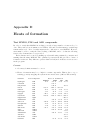
D Heats of formation
151
E References
153
CONTENTS
• New Functionalities:
– Michael B. Coolidge, The Frank J. Seiler Research Laboratory, U.S. Air
Force Academy, CO 80840, and James J. P. Stewart, Stewart Computational
Chemistry, 15210 Paddington Circle, Colorado Springs, CO 80921-2512. (The
Air Force code was obtained under the Freedom of Information Act)
Symmetry is used to speed up FORCE calculations, and to facilitate the analysis of molecular vibrations.
– David Danovich, The Fritz Haber Research Center for Molecular Dynamics,
The Hebrew University of Jerusalem, 91904 Jerusalem, Israel.
Ionization potentials are corrected using Green’s Function techniques. The
resulting I.P.s are generally more accurate than the conventional I.P.s.
The point–group of the system is identified, and molecular orbitals are characterized by irreducible representation.
– Andreas Klamt Bayer AG, Q18, D-5090 Leverkusen-Beyerwerk, Germany.
A new approach to dielectric screening in solvents with explicit expressions for
the screening energy and its gradient has been added.
• Existing Functionalities:
– Victor I. Danilov, Department of Quantum Biophysics, Academy of Sciences of the Ukraine, Kiev 143, Ukraine.
Edited the MOPAC 7 Manual, and provided the basis for Section 6.17.2, on
excited states.
– Henry Kurtz and Prakashan Korambath, Department of Chemistry,
Memphis State University, Memphis TN 38152.
The Hyperpolarizability calculation, originally written by Prof Kurtz, has been
improved so that frequency dependent non-linear optical calculations can be
performed. (Prakashan Korambath, dissertation research)
– Frank Jensen, Department of Chemistry, Odense Universitet, Campusvej
55, DK–5230 Odense M, Denmark.
The efficiency of Baker’s EF routine has been improved.
– John M. Simmie, Chemistry Department, University College, Galway, Ireland.
The MOPAC Manual has been completely re-formatted in the LaTeX document
preparation system. Equations are now much easier to read and to understand.
– Jorge A. Medrano, 5428 Falcon Ln., West Chester, OH 45069, and Roberto
Bochicchio (Universidad de Buenos Aires).
The BONDS function has been extended to allow free valence and other quantities to be calculated.
– George Purvis III, CAChe Scientific, P.O. Box 500, Delivery Station 13400, Beaverton, OR 97077.
The STO-6G Gaussian expansion of the Slater orbitals has been expanded
to Principal Quantum Number 6. These expansions are used in analytical
derivative calculations.
• Bug-reports/bug-fixes:
– Victor I. Danilov, Department of Quantum Biophysics, Academy of Sciences of the Ukraine, Kiev 143, Ukraine.
Several faults in the multi-electron configuration interaction were identified,
and recommendations made regarding their correction.
CONTENTS
Chapter 1
Description of MOPAC
MOPAC is a general-purpose semi-empirical molecular orbital package for the study of
chemical structures and reactions. The semi-empirical Hamiltonians MNDO, MINDO/3,
AM1, and PM3 are used in the electronic part of the calculation to obtain molecular
orbitals, the heat of formation and its derivative with respect to molecular geometry.
Using these results MOPAC calculates the vibrational spectra, thermodynamic quantities,
isotopic substitution effects and force constants for molecules, radicals, ions, and polymers.
For studying chemical reactions, a transition state location routine and two transition
state optimizing routines are available. For users to get the most out of the program,
they must understand how the program works, how to enter data, how to interpret the
results, and what to do when things go wrong.
While MOPAC calls upon many concepts in quantum theory and thermodynamics
and uses some fairly advanced mathematics, the user need not be familiar with these
specialized topics. MOPAC is written with the non-theoretician in mind. The input data
are kept as simple as possible so users can give their attention to the chemistry involved
and not concern themselves with quantum and thermodynamic exotica.
The simplest description of how MOPAC works is that the user creates a data-file
which describes a molecular system and specifies what kind of calculations and output
are desired. The user then commands MOPAC to carry out the calculation using that
data-file. Finally the user extracts the desired output on the system from the output files
created by MOPAC.
1. This is the “sixth edition”. MOPAC has undergone a steady expansion since its first
release, and users of the earlier editions are recommended to familiarize themselves
with the changes which are described in this manual. If any errors are found, or
if MOPAC does not perform as described, please contact Dr. James J. P. Stewart,
Frank J. Seiler Research Laboratory, U.S. Air Force Academy, Colorado Springs,
CO 80840–6528.
2. MOPAC runs successfully on normal CDC, Data General, Gould, and DEC computers, and also on the CDC 205 and CRAY–XMP “supercomputers”. The CRAY
version has been partly optimized to take advantage of the CRAY architecture.
Several versions exist for microcomputers such as the IBM PC-AT and XT, Zenith,
etc.
1.1
Summary of MOPAC capabilities
1. MNDO, MINDO/3, AM1, and PM3 Hamiltonians.
2. Restricted Hartree-Fock (RHF) and Unrestricted Hartree-Fock (UHF) methods.
3. Extensive Configuration Interaction
Description of MOPAC
(a) 100 configurations
(b) Singlets, Doublets, Triplets, Quartets, Quintets, and Sextets
(c) Excited states
(d) Geometry optimizations, etc., on specified states
4. Single SCF calculation
5. Geometry optimization
6. Gradient minimization
7. Transition state location
8. Reaction path coordinate calculation
9. Force constant calculation
10. Normal coordinate analysis
11. Transition dipole calculation
12. Thermodynamic properties calculation
13. Localized orbitals
14. Covalent bond orders
15. Bond analysis into sigma and pi contributions
16. One dimensional polymer calculation
17. Dynamic Reaction Coordinate calculation
18. Intrinsic Reaction Coordinate calculation
1.2
Copyright status of MOPAC
At the request of the Air Force Academy Law Department the following notice has been
placed in MOPAC.
Notice of Public Domain nature of MOPAC.
“This computer program is a work of the United States Government and as
such is not subject to protection by copyright (17 U.S.C. # 105.) Any person
who fraudulently places a copyright notice or does any other act contrary to
the provisions of 17 U.S. Code 506(c) shall be subject to the penalties provided
therein. This notice shall not be altered or removed from this software and is
to be on all reproductions.”
I recommend that a user obtain a copy by either copying it from an existing site or
ordering an ‘official’ copy from the Quantum Chemistry Program Exchange, (QCPE),
Department of Chemistry, Indiana University, Bloomington, Indiana, 47405. The cost
covers handling only. Contact the Editor, Richard Counts, at (812) 855–4784 for further
details.
1.3 Porting MOPAC to other machines
1.3
Porting MOPAC to other machines
MOPAC is written for the DIGITAL VAX computer. However, the program has been
written with the idea that it will be ported to other machines. After such a port has
been done, the new program should be given the version number 6.10, or, if two or more
versions are generated, 6.20, 6.30, etc. To validate the new copy, QCPE has a test-suite
of calculations. If all tests are passed, within the tolerances given in the tests, then the
new program can be called a valid version of MOPAC 6. Insofar as is practical, the mode
of submission of a MOPAC job should be preserved, e.g.,
(prompt) MOPAC <data-set> [<queue-options>...]
Any changes which do not violate the FORTRAN–77 conventions, and which users
believe would be generally desirable, can be sent to the author.
1.4
Relationship of AMPAC and MOPAC
In 1985 MOPAC 3.0 and AMPAC 1.0 were submitted to QCPE for distribution. At that
time, AMPAC differed from MOPAC in that it had the AM1 algorithm. Additionally,
changes in some MNDO parameters in AMPAC made AMPAC results incompatable with
MOPAC Versions 1-3. Subsequent versions of MOPAC, in addition to being more highly
debugged than Version 3.0, also had the AM1 method. Such versions were compatible
with AMPAC and with versions 1–3 of MOPAC.
In order to avoid confusion, all versions of MOPAC after 3.0 include journal references
so that the user knows unambiguously which parameter sets were used in any given job.
Since 1985 AMPAC and MOPAC have evolved along different lines. In MOPAC I
have endeavoured to provide a highly robust program, one with only a few new features,
but which is easily portable and which can be relied upon to give precise, if not very
exciting, answers. At Austin, the functionality of AMPAC has been enhanced by the
research work of Prof. Dewar’s group. The new AMPAC 2.1 thus has functionalities not
present in MOPAC. In publications, users should cite not only the program name but also
the version number.
Commercial concerns have optimized both MOPAC and AMPAC for use on supercomputers. The quality of optimization and the degree to which the parent algorithm
has been preserved differs between MOPAC and AMPAC and also between some machine
specific versions. Different users may prefer one program to the other, based on considerations such as speed. Some modifications of AMPAC run faster than some modifications
of MOPAC, and vice versa, but if these are modified versions of MOPAC 3.0 or AMPAC
1.0, they represent the programming prowess of the companies doing the conversion, and
not any intrinsic difference between the two programs.
Testing of these large algorithms is difficult, and several times users have reported
bugs in MOPAC or AMPAC which were introduced after they were supplied by QCPE.
Cooperative Development of MOPAC
MOPAC has developed, and hopefully will continue to develop, by the addition of contributed code. As a policy, any supplied code which is incorporated into MOPAC will be
described in the next release of the Manual, and the author or supplier acknowledged. In
the following release only journal references will be retained. The objective is to produce
a good program. This is obviously not a one-person undertaking; if it was, then the product would be poor indeed. Instead, as we are in a time of rapid change in computational
chemistry, a time characterized by a very free exchange of ideas and code, MOPAC has
been evolving by accretion. The unstinting and generous donation of intellectual effort
speaks highly of the donors. However, with the rapid commercialization of computational
Description of MOPAC
chemistry software in the past few years, it is unfortunate but it seems unlikely that this
idyllic state will continue.
1.5
Programs recommended for use with MOPAC
MOPAC is the core program of a series of programs for the theoretical study of chemical
phenomena. This version is the sixth in an on-going development, and efforts are being
made to continue its further evolution. In order to make using MOPAC easier, five other
programs have also been written. Users of MOPAC are recommended to use all four
programs. Efforts will be made to continue the development of these programs.
HELP
HELP is a stand-alone program which mimics the VAX HELP function. It is intended for
users on UNIX computers. HELP comes with the basic MOPAC 6.00, and is recommended
for general use.
DRAW
DRAW, written by Maj. Donn Storch, USAF, and available through QCPE, is a powerful editing program specifically written to interface with MOPAC. Among the various
facilities it offers are:
1. The on-line editing and analysis of a data file, starting from scratch or from an
existing data file, an archive file, or from a results file.
2. The option of continuous graphical representation of the system being studied.
Several types of terminals are supported, including DIGITAL, TEKTRONIX, and
TERAK terminals.
3. The drawing of electron density contour maps generated by DENSITY on graphical
devices.
4. The drawing of solid-state band structures generated by MOSOL.
5. The sketching of molecular vibrations, generated by a normal coordinate analysis.
DENSITY
DENSITY, written by Dr. James J. P. Stewart, and available through QCPE, is an
electron-density plotting program. It accepts data-files directly from MOPAC, and is
intended to be used for the graphical representation of electron density distribution, individual M.O.’s, and difference maps.
MOHELP
MOHELP, also available through QCPE, is an on-line help facility, written by Maj. Donn
Storch and Dr. James J. P. Stewart, to allow non-VAX users access to the VAX HELP
libraries for MOPAC, DRAW, and DENSITY.
MOSOL
MOSOL (Distributed by QCPE) is a full solid-state MNDO program written by Dr.
James J. P. Stewart. In comparison with MOPAC, MOSOL is extremely slow. As a
result, while geometry optimization, force constants, and other functions can be carried
out by MOSOL, these slow calculations are best done using the solid-state facility within
MOPAC. MOSOL should be used for two or three dimensional solids only, a task that
MOPAC cannot perform.
1.6 The data-file
1.6
The data-file
This section is aimed at the complete novice — someone who knows nothing at all about
the structure of a MOPAC data-file.
First of all, there are at most four possible types of data-files for MOPAC, but the
simplest data-file is the most commonly used. Rather than define it, two examples are
shown below. An explanation of the geometry definitions shown in the examples is given
in the chapter “GEOMETRY SPECIFICATION”.
1.6.1
Example of data for ethylene
Line
Line
Line
Line
Line
Line
Line
Line
Line
Line
1 :
2 :
3 :
4a:
4b:
4c:
4d:
4e:
4f:
5 :
UHF PULAY MINDO3 VECTORS DENSITY LOCAL T=300
EXAMPLE OF DATA FOR MOPAC
MINDO/3 UHF CLOSED-SHELL D2D ETHYLENE
C
C
H
H
H
H
1.400118
1.098326
1.098326
1.098326
1.098326
1
1
1
1
1
123.572063
123.572063
123.572063
123.572063
1
1
1
1
180.000000
90.000000
270.000000
0
0
0
2
1
1
1
2
2
As can be seen, the first three lines are textual. The first line consists of keywords
(here seven keywords are shown). These control the calculation. The next two lines are
comments or titles. The user might want to put the name of the molecule and why it is
being run on these two lines.
These three lines are obligatory. If no name or comment is wanted, leave blank lines.
If no keywords are specified, leave a blank line. A common error is to have a blank line
before the keyword line: this error is quite tricky to find, so be careful not to have four
lines before the start of the geometric data (lines 4a-4f in the example). Whatever is
decided, the three lines, blank or otherwise, are obligatory.
In the example given, one line of keywords and two of documentation are shown.
By use of keywords, these defaults can be changed. Modifying keywords are +, &, and
SETUP. These are defined in the KEYWORDS chapter. The following table illustrates
the allowed combinations:
Line 1
Line 2
Keys
Keys
Keys
Keys
Keys
Keys
Keys
Keys
Text
Keys
Keys
Keys
Keys
Text
Keys
Keys
+
+
&
&
SETUP
+
&
Line 3
Text
Text
+
Keys
Text
&
Keys
Text
SETUP Text
SETUP Text
Line 4
Z-matrix
Text
Text
Z-matrix
Z-matrix
Z-matrix
Text
Z-matrix
Line 5
Setup used
Z-matrix not used
Z-matrix not used
Text
not used
Z-matrix not used
Z-matrix not used
Z-matrix 1 or 2 lines used
Z-matrix 1 line used
Z-matrix 1 line used
No other combinations are allowed.
The proposed use of the SETUP option is to allow a frequently used set of keywords
to be defined by a single keyword. For example, if the default criteria are not suitable,
SETUP might contain:
" SCFCRT=1.D-8
"
SHIFT=30 ITRY=600 GNORM=0.02 ANALYT "
"
3
3
3
Description of MOPAC
The order of usage of a keyword is:
Line 1 > Line 2 > Line 3.
Line 1 > SETUP.
Line 2 > SETUP.
SETUP > built in default values.
The next set of lines defines the geometry. In the example, the numbers are all neatly
lined up; this is not necessary, but does make it easier when looking for errors in the data.
The geometry is defined in lines 4a to 4f; line 5 terminates both the geometry and the
data-file. Any additional data, for example symmetry data, would follow line 5.
Summarizing, then, the structure for a MOPAC data-file is:
Line 1 Keywords. (See chapter 2 on definitions of keywords)
Line 2 Title of the calculation, e.g. the name of the molecule or ion.
Line 3 Other information describing the calculation.
Lines 4 Internal or cartesian coordinates (See chapter on specification of geometry)
Line 5 Blank line to terminate the geometry definition.
Other layouts for data-files involve additions to the simple layout. These additions
occur at the end of the data-file, after line 5. The three most common additions are:
• Symmetry data: This follows the geometric data, and is ended by a blank line.
• Reaction path: After all geometry and symmetry data (if any) are read in, points
on the reaction coordinate are defined.
• Saddle data: A complete second geometry is input. The second geometry follows
the first geometry and symmetry data (if any).
1.6.2
Example of data for polytetrahydrofuran
The following example illustrates the data file for a four hour polytetrahydrofuran calculation. As you can see the layout of the data is almost the same as that for a molecule,
the main difference is in the presence of the translation vector atom “Tv”.
Line
Line
Line
Line
Line
Line
Line
Line
Line
Line
Line
Line
Line
Line
Line
Line
Line
Line
1 :T=4H
2 :
3 :
4a:
C
4b:
C
4c:
O
4d:
C
4e:
C
4f:
C
4g:
C
4h:
O
4i:
C
4j:
C
4k: XX
4l: XX
4m:
H
4n:
H
4o:
H
POLY-TETRAHYDROFURAN (C4 H8 O)2
0.000000
1.551261
1.401861
1.401958
1.551074
1.541928
1.551502
1.402677
1.402671
1.552020
1.552507
1.547723
1.114250
1.114708
1.123297
0
1
1
1
1
1
1
1
1
1
1
1
1
1
1
0.000000
0.000000
108.919034
119.302489
108.956238
113.074843
113.039652
108.663575
119.250433
108.665746
112.659354
113.375266
89.824605
89.909148
93.602831
0
0
1
1
1
1
1
1
1
1
1
1
1
1
1
0.000000
0.000000
0.000000
-179.392581
179.014664
179.724877
179.525806
179.855864
-179.637345
-179.161900
-178.914985
-179.924995
126.911018
-126.650667
127.182594
0
0
0
1
1
1
1
1
1
1
1
1
1
1
1
0 0
1 0
2 1
3 2
4 3
5 4
6 5
7 6
8 7
9 8
10 9
11 10
1 3
1 3
2 4
0
0
0
1
2
3
4
5
6
7
8
9
2
2
3
1.6 The data-file
Line
Line
Line
Line
Line
Line
Line
Line
Line
Line
Line
Line
Line
Line
Line
4p:
4q:
4r:
4s:
4t:
4u:
4v:
4w:
4x:
4y:
4z:
4A:
4B:
4C:
5 :
H
H
H
H
H
H
H
H
H
H
H
H
H
Tv
0
1.123640
1.123549
1.123417
1.114352
1.114462
1.114340
1.114433
1.123126
1.123225
1.123328
1.123227
1.113970
1.114347
12.299490
0.000000
1
1
1
1
1
1
1
1
1
1
1
1
1
1
0
93.853406
90.682924
90.679889
90.239157
89.842852
89.831790
89.753913
93.644744
93.880969
90.261019
91.051403
90.374545
90.255788
0.000000
0.000000
1
1
1
1
1
1
1
1
1
1
1
1
1
0
0
-126.320187
126.763659
-127.033695
126.447043
-127.140168
126.653999
-126.926618
127.030541
-126.380511
127.815464
-125.914234
126.799259
-126.709810
0.000000
0.000000
1
1
1
1
1
1
1
1
1
1
1
1
1
0
0
2
4
4
5
5
6
6
7
7
9
9
10
10
1
0
4
6
6
7
7
8
8
9
9
11
11
12
12
11
0
3
5
5
6
6
7
7
8
8
10
10
11
11
10
0
Polytetrahydrofuran has a repeat unit of (C4 H8 O)2 ; i.e., twice the monomer unit.
This is necessary in order to allow the lattice to repeat after a translation through 12.3 ˚
A.
See the section on Solid State Capability for further details.
Note the two dummy atoms on lines 4k and 4l. These are useful, but not essential,
for defining the geometry. The atoms on lines 4y to 4B use these dummy atoms, as does
the translation vector on line 4C. The translation vector has only the length marked for
optimization. The reason for this is also explained in the Background chapter.
Description of MOPAC
Chapter 2
Keywords
2.1
Specification of keywords
All control data are entered in the form of keywords, which form the first line of a datafile. A description of what each keyword does is given in Section 2.3. The order in
which keywords appear is not important although they must be separated by a space.
Some keywords can be abbreviated, allowed abbreviations are noted in Section 2.3 (for
example 1ELECTRON can be entered as 1ELECT). However the full keyword is preferred
in order to more clearly document the calculation and to obviate the possibility that an
abbreviated keyword might not be recognized. If there is insufficient space in the first
line for all the keywords needed, then consider abbreviating the longer words. One type
of keyword, those with an equal sign, such as, BAR=0.05, may not be abbreviated, and
the full word needs to be supplied.
Most keywords which involve an equal sign, such as SCFCRT=1.D-12 can, at the user’s
discretion, be written with spaces before and after the equal sign. Thus all permutations of SCFCRT=1.D-12, such as SCFCRT =1.D-12, SCFCRT = 1.D-12, SCFCRT= 1.D-12,
SCFCRT = 1.D-12, etc. are allowed. Exceptions to this are T=, T-PRIORITY=, HPRIORITY=, X-PRIORITY=, IRC=, DRC= and TRANS=. ‘ T=’ cannot be abbreviated to ‘ T ’ as many keywords start or end with a ‘T’; for the other keywords the
associated abbreviated keywords have specific meanings.
If two keywords which are incompatible, like UHF and C.I., are supplied, or a keyword
which is incompatible with the species supplied, for instance TRIPLET and a methyl
radical, then error trapping will normally occur, and an error message will be printed.
This usually takes an insignificant time, so data are quickly checked for obvious errors.
2.2
Full list of keywords used in MOPAC
&
+
0SCF
1ELECTRON1SCF
AIDER
AIGIN
AIGOUT
ANALYT
AM1
BAR=n.n BIRADICALBONDS
C.I.
-
TURN NEXT LINE INTO KEYWORDS
ADD ANOTHER LINE OF KEYWORDS
READ IN DATA, THEN STOP
PRINT FINAL ONE-ELECTRON MATRIX
DO ONE SCF AND THEN STOP
READ IN AB INITIO DERIVATIVES
GEOMETRY MUST BE IN GAUSSIAN FORMAT
IN ARC FILE, INCLUDE AB-INITIO GEOMETRY
USE ANALYTICAL DERIVATIVES OF ENERGY WRT GEOMETRY
USE THE AM1 HAMILTONIAN
REDUCE BAR LENGTH BY A MAXIMUM OF n.n
SYSTEM HAS TWO UNPAIRED ELECTRONS
PRINT FINAL BOND-ORDER MATRIX
A MULTI-ELECTRON CONFIGURATION INTERACTION SPECIFIED
Keywords
CHARGE=n
COMPFG
CONNOLLY
DEBUG
DENOUT
DENSITY
DEP
DEPVAR=n
DERIV
DFORCE
DFP
DIPOLE
DIPX
DIPY
DIPZ
DMAX
DOUBLET
DRC
DUMP=n
ECHO
EF
EIGINV
EIGS
ENPART
ESP
ESPRST
ESR
EXCITED
EXTERNAL
FILL=n
-
FLEPO
FMAT
FOCK
FORCE
GEO-OK
GNORM=n.nGRADIENTSGRAPH
HCORE
HESS=N
H-PRIO
HYPERFINEIRC
ISOTOPE ITER
ITRY=N
IUPD
K=(N,N) KINETIC LINMIN
LARGE
LET
LOCALIZE -
CHARGE ON SYSTEM = n (e.g. NH4 => CHARGE=1)
PRINT HEAT OF FORMATION CALCULATED IN COMPFG
USE CONNOLLY SURFACE
DEBUG OPTION TURNED ON
DENSITY MATRIX OUTPUT (CHANNEL 10)
PRINT FINAL DENSITY MATRIX
GENERATE FORTRAN CODE FOR PARAMETERS FOR NEW ELEMENTS
TRANSLATION VECTOR IS A MULTIPLE OF BOND-LENGTH
PRINT PART OF WORKING IN DERIV
FORCE CALCULATION SPECIFIED, ALSO PRINT FORCE MATRIX.
USE DAVIDON-FLETCHER-POWELL METHOD TO OPTIMIZE GEOMETRIES
FIT THE ESP TO THE CALCULATED DIPOLE
X COMPONENT OF DIPOLE TO BE FITTED
Y COMPONENT OF DIPOLE TO BE FITTED
Z COMPONENT OF DIPOLE TO BE FITTED
MAXIMUM STEPSIZE IN EIGENVECTOR FOLLOWING
DOUBLET STATE REQUIRED
DYNAMIC REACTION COORDINATE CALCULATION
WRITE RESTART FILES EVERY n SECONDS
DATA ARE ECHOED BACK BEFORE CALCULATION STARTS
USE EF ROUTINE FOR MINIMUM SEARCH
PRINT ALL EIGENVALUES IN ITER
PARTITION ENERGY INTO COMPONENTS
ELECTROSTATIC POTENTIAL CALCULATION
RESTART OF ELECTROSTATIC POTENTIAL
CALCULATE RHF UNPAIRED SPIN DENSITY
OPTIMIZE FIRST EXCITED SINGLET STATE
READ PARAMETERS OFF DISK
IN RHF OPEN AND CLOSED SHELL, FORCE M.O. n
TO BE FILLED
PRINT DETAILS OF GEOMETRY OPTIMIZATION
PRINT DETAILS OF WORKING IN FMAT
PRINT LAST FOCK MATRIX
FORCE CALCULATION SPECIFIED
OVERRIDE INTERATOMIC DISTANCE CHECK
EXIT WHEN GRADIENT NORM DROPS BELOW n.n
PRINT ALL GRADIENTS
GENERATE FILE FOR GRAPHICS
PRINT DETAILS OF WORKING IN HCORE
OPTIONS FOR CALCULATING HESSIAN MATRICES IN EF
HEAT OF FORMATION TAKES PRIORITY IN DRC
HYPERFINE COUPLING CONSTANTS TO BE CALCULATED
INTRINSIC REACTION COORDINATE CALCULATION
FORCE MATRIX WRITTEN TO DISK (CHANNEL 9 )
PRINT DETAILS OF WORKING IN ITER
SET LIMIT OF NUMBER OF SCF ITERATIONS TO N.
MODE OF HESSIAN UPDATE IN EIGENVECTOR FOLLOWING
BRILLOUIN ZONE STRUCTURE TO BE CALCULATED
EXCESS KINETIC ENERGY ADDED TO DRC CALCULATION
PRINT DETAILS OF LINE MINIMIZATION
PRINT EXPANDED OUTPUT
OVERRIDE CERTAIN SAFETY CHECKS
PRINT LOCALIZED ORBITALS
2.2 Full list of keywords used in MOPAC
MAX
MECI
MICROS
MINDO/3
MMOK
MODE=N
MOLDAT
MS=N
MULLIK
NLLSQ
NOANCI
NODIIS
NOINTER
NOLOG
NOMM
NONR
NOTHIEL
NSURF=N
NOXYZ
NSURF
OLDENS
OLDGEO
OPEN
ORIDE
PARASOK
PI
PL
PM3
POINT=N
POINT1=N
POINT2=N
POLAR
POTWRT
POWSQ
PRECISE
PULAY
QUARTET
QUINTET
RECALC=N
RESTART
ROOT=n
ROT=n
SADDLE
SCALE
SCFCRT=n
SCINCR
SETUP
SEXTET
SHIFT=n
SIGMA
SINGLET
SLOPE
SPIN
STEP
-
PRINTS MAXIMUM GRID SIZE (23*23)
PRINT DETAILS OF MECI CALCULATION
USE SPECIFIC MICROSTATES IN THE C.I.
USE THE MINDO/3 HAMILTONIAN
USE MOLECULAR MECHANICS CORRECTION TO CONH BONDS
IN EF, FOLLOW HESSIAN MODE NO. N
PRINT DETAILS OF WORKING IN MOLDAT
IN MECI, MAGNETIC COMPONENT OF SPIN
PRINT THE MULLIKEN POPULATION ANALYSIS
MINIMIZE GRADIENTS USING NLLSQ
DO NOT USE ANALYTICAL C.I. DERIVATIVES
DO NOT USE DIIS GEOMETRY OPTIMIZER
DO NOT PRINT INTERATOMIC DISTANCES
SUPPRESS LOG FILE TRAIL, WHERE POSSIBLE
DO NOT USE MOLECULAR MECHANICS CORRECTION TO CONH BONDS
DO NOT USE THIEL’S FSTMIN TECHNIQUE
NUMBER OF SURFACES IN AN ESP CALCULATION
DO NOT PRINT CARTESIAN COORDINATES
NUMBER OF LAYERS USED IN ELECTROSTATIC POTENTIAL
READ INITIAL DENSITY MATRIX OFF DISK
PREVIOUS GEOMETRY TO BE USED
OPEN-SHELL RHF CALCULATION REQUESTED
IN AM1 CALCULATIONS SOME MNDO PARAMETERS ARE TO BE USED
RESOLVE DENSITY MATRIX INTO SIGMA AND PI BONDS
MONITOR CONVERGENCE OF DENSITY MATRIX IN ITER
USE THE MNDO-PM3 HAMILTONIAN
NUMBER OF POINTS IN REACTION PATH
NUMBER OF POINTS IN FIRST DIRECTION IN GRID CALCULATION
NUMBER OF POINTS IN SECOND DIRECTION IN GRID CALCULATION
CALCULATE FIRST, SECOND AND THIRD ORDER POLARIZABILITIES
IN ESP, WRITE OUT ELECTROSTATIC POTENTIAL TO UNIT 21
PRINT DETAILS OF WORKING IN POWSQ
CRITERIA TO BE INCREASED BY 100 TIMES
USE PULAY’S CONVERGER TO OBTAIN A SCF
QUARTET STATE REQUIRED
QUINTET STATE REQUIRED
IN EF, RECALCULATE HESSIAN EVERY N STEPS
CALCULATION RESTARTED
ROOT n TO BE OPTIMIZED IN A C.I. CALCULATION
THE SYMMETRY NUMBER OF THE SYSTEM IS n.
OPTIMIZE TRANSITION STATE
SCALING FACTOR FOR VAN DER WAALS DISTANCE IN ESP
DEFAULT SCF CRITERION REPLACED BY THE VALUE SUPPLIED
INCREMENT BETWEEN LAYERS IN ESP
EXTRA KEYWORDS TO BE READ OF SETUP FILE
SEXTET STATE REQUIRED
A DAMPING FACTOR OF n DEFINED TO START SCF
MINIMIZE GRADIENTS USING SIGMA
SINGLET STATE REQUIRED
MULTIPLIER USED TO SCALE MNDO CHARGES
PRINT FINAL UHF SPIN MATRIX
STEP SIZE IN PATH
Keywords
STEP1=n
STEP2=n
STO-3G
SYMAVG
SYMMETRY
T=n
THERMO
TIMES
T-PRIO
TRANS
-
TRIPLET
TS
UHF
VECTORS
VELOCITY
WILLIAMS
X-PRIO
XYZ
-
2.3
STEP SIZE n FOR FIRST COORDINATE IN GRID CALCULATION
STEP SIZE n FOR SECOND COORDINATE IN GRID CALCULATION
DEORTHOGONALIZE ORBITALS IN STO-3G BASIS
AVERAGE SYMMETRY EQUIVALENT ESP CHARGES
IMPOSE SYMMETRY CONDITIONS
A TIME OF n SECONDS REQUESTED
PERFORM A THERMODYNAMICS CALCULATION
PRINT TIMES OF VARIOUS STAGES
TIME TAKES PRIORITY IN DRC
THE SYSTEM IS A TRANSITION STATE
(USED IN THERMODYNAMICS CALCULATION)
TRIPLET STATE REQUIRED
USING EF ROUTINE FOR TS SEARCH
UNRESTRICTED HARTREE-FOCK CALCULATION
PRINT FINAL EIGENVECTORS
SUPPLY THE INITIAL VELOCITY VECTOR IN A DRC CALCULATION
USE WILLIAMS SURFACE
GEOMETRY CHANGES TAKE PRIORITY IN DRC
DO ALL GEOMETRIC OPERATIONS IN CARTESIAN COORDINATES.
Definitions of keywords
The definitions below are given with some technical expressions which are not further
defined. Interested users are referred to Appendix E of this manual to locate appropriate
references which will provide further clarification.
There are three classes of keywords:
1. those which CONTROL substantial aspects of the calculation, i.e., those which
affect the final heat of formation,
2. those which determine which OUTPUT will be calculated and printed, and
3. those which dictate the WORKING of the calculation, but which do not affect the
heat of formation. The assignment to one of these classes is designated by a (C),
(O) or (W), respectively, following each keyword in the list below.
& (C)
An ‘ &’ means ‘turn the next line into keywords’. Note the space before the ‘&’ sign.
Since ‘&’ is a keyword, it must be preceeded by a space. A ‘ &’ on line 1 would mean
that a second line of keywords should be read in. If that second line contained a ‘ &’,
then a third line of keywords would be read in. If the first line has a ‘ &’ then the first
description line is omitted, if the second line has a ‘ &’, then both description lines are
omitted.
Examples: Use of one ‘&’
VECTORS DENSITY RESTART & NLLSQ T=1H SCFCRT=1.D-8 DUMP=30M ITRY=300
PM3 FOCK OPEN(2,2) ROOT=3 SINGLET SHIFT=30
Test on a totally weird system: Use of two ‘&’s
LARGE=-10 & DRC=4.0 T=1H SCFCRT=1.D-8 DUMP=30M ITRY=300 SHIFT=30
PM3 OPEN(2,2) ROOT=3 SINGLET NOANCI ANALYT T-PRIORITY=0.5 &
LET GEO-OK VELOCITY KINETIC=5.0
2.3 Definitions of keywords
+ (C)
A ‘ +’ sign means ‘read another line of keywords’. Note the space before the ‘+’ sign.
Since ‘+’ is a keyword, it must be preceeded by a space. A ‘ +’ on line 1 would mean
that a second line of keywords should be read in. If that second line contains a ‘ +’, then
a third line of keywords will be read in. Regardless of whether a second or a third line of
keywords is read in, the next two lines would be description lines.
Example of ‘ +’ option
RESTART T=4D FORCE OPEN(2,2) SHIFT=20 PM3 +
SCFCRT=1.D-8 DEBUG + ISOTOPE FMAT ECHO singlet ROOT=3
THERMO(300,400,1) ROT=3
Example of data set with three lines of keywords. Note: There are two lines of
description, this and the previous line.
0SCF (O)
The data can be read in and output, but no actual calculation is performed when this
keyword is used. This is useful as a check on the input data. All obvious errors are
trapped, and warning messages printed.
A second use is to convert from one format to another. The input geometry is printed
in various formats at the end of a 0SCF calculation. If NOINTER is absent, cartesian coordinates are printed. Unconditionally, MOPAC Z-matrix internal coordinates are
printed, and if AIGOUT is present, Gaussian Z-matrix internal coordinates are printed.
0SCF should now be used in place of DDUM.
1ELECTRON (O)
The final one-electron matrix is printed out. This matrix is composed of atomic orbitals;
the array element between orbitals i and j on different atoms is given by:
H(i, j) = 0.5 × (βi + βj ) × overlap(i, j)
The matrix elements between orbitals i and j on the same atom are calculated from
the electron-nuclear attraction energy, and also from the U (i) value if i = j.
The one-electron matrix is unaffected by (a) the charge and (b) the electron density.
It is only a function of the geometry. Abbreviation: 1ELEC.
1SCF (C)
When users want to examine the results of a single SCF calculation of a geometry, 1SCF
should be used. 1SCF can be used in conjunction with RESTART, in which case a single
SCF calculation will be done, and the results printed.
When 1SCF is used on its own (that is, RESTART is not also used) then derivatives
will only be calculated if GRAD is also specified.
1SCF is helpful in a learning situation. MOPAC normally performs many SCF calculations, and in order to minimize output when following the working of the SCF calculation,
1SCF is very useful.
AIDER (C)
AIDER allows MOPAC to optimize an ab-initio geometry. To use it, calculate the ab-initio
gradients using, e.g., Gaussian. Supply MOPAC with these gradients, after converting
them into kcal/mol. The geometry resulting from a MOPAC run will be nearer to the
optimized ab-initio geometry than if the geometry optimizer in Gaussian had been used.
Keywords
AIGIN (C)
If the geometry (Z-matrix) is specified using the Gaussian-8X, then normally this will be
read in without difficulty. In the event that it is mistaken for a normal MOPAC-type
Z-matrix, the keyword AIGIN is provided. AIGIN will force the data-set to be read in
assuming Gaussian format. This is necessary if more than one system is being studied in
one run.
AIGOUT (O)
The ARCHIVE file contains a data-set suitable for submission to MOPAC. If, in addition
to this data-set, the Z-matrix for Gaussian input is wanted, then AIGOUT (ab initio
geometry output), should be used.
The Z-matrix is in full Gaussian form. Symmetry, where present, will be correctly defined. Names of symbolics will be those used if the original geometry was in Gaussian format, otherwise ‘logical’ names will be used. Logical names are of form <t><a><b>[<c>][<d>]
where <t> is ‘r’ for bond length, ‘a’ for angle, or ‘d’ for dihedral, <a> is the atom number,
<b> is the atom to which <a> is related, <c>, if present, is the atom number to which <a>
makes an angle, and <d>, if present, is the atom number to which <a> makes a dihedral.
ANALYT (W)
By default, finite difference derivatives of energy with respect to geometry are used. If
ANALYT is specified, then analytical derivatives are used instead. Since the analytical
derivatives are over Gaussian functions—a STO-6G basis set is used—the overlaps are
also over Gaussian functions. This will result in a very small (less than 0.1 kcal/mole)
change in heat of formation. Use analytical derivatives (a) when the mantissa used is less
than about 51–53 bits, or (b) when comparison with finite difference is desired. Finite
difference derivatives are still used when non-variationally optimized wavefunctions are
present.
AM1 (C)
The AM1 method is to be used. By default MNDO is run.
BAR=n.nn (W)
In the SADDLE calculation the distance between the two geometries is steadily reduced
until the transition state is located. Sometimes, however, the user may want to alter the
maximum rate at which the distance between the two geometries reduces. BAR is a ratio,
normally 0.15, or 15 percent. This represents a maximum rate of reduction of the bar
of 15 percent per step. Alternative values that might be considered are BAR=0.05 or
BAR=0.10, although other values may be used. See also SADDLE.
If CPU time is not a major consideration, use BAR=0.03.
BIRADICAL (C)
Note: BIRADICAL is a redundant keyword, and represents a particular configuration
interaction calculation. Experienced users of MECI (q.v.) can duplicate the effect of the
keyword BIRADICAL by using the MECI keywords OPEN(2,2) and SINGLET.
For molecules which are believed to have biradicaloid character the option exists to
optimize the lowest singlet energy state which results from the mixing of three states.
These states are, in order, (1) the (micro)state arising from a one electron excitation
from the HOMO to the LUMO, which is combined with the microstate resulting from
the time-reversal operator acting on the parent microstate, the result being a full singlet
state; (2) the state resulting from de-excitation from the formal LUMO to the HOMO;
2.3 Definitions of keywords
and (3) the state resulting from the single electron in the formal HOMO being excited
into the LUMO.
Microstate 1
Alpha Beta
LUMO
*
---
Alpha Beta
---
---
Microstate 2
Microstate 3
Alpha
Alpha
*
---
---
---
*
---
Beta
Beta
---
*
---
*
---
*
---
---
---
+
HOMO
---
*
---
*
---
A configuration interaction calculation is involved here. A biradical calculation done
without C.I. at the RHF level would be meaningless. Either rotational invariance would
be lost, as in the D2d form of ethylene, or very artificial barriers to rotations would
be found, such as in a methane molecule “orbiting” a D2d ethylene. In both cases the
inclusion of limited configuration interaction corrects the error. BIRADICAL should not
be used if either the HOMO or LUMO is degenerate; in this case, the full manifold of
HOMO × LUMO should be included in the C.I., using MECI options. The user should be
aware of this situation. When the biradical calculation is performed correctly, the result
is normally a net stabilization. However, if the first singlet excited state is much higher
in energy than the closed-shell ground state, BIRADICAL can lead to a destabilization.
Abbreviation: BIRAD. See also MECI, C.I., OPEN, SINGLET.
BONDS (O)
The rotationally invariant bond order between all pairs of atoms is printed. In this context
a bond is defined as the sum of the squares of the density matrix elements connecting
any two atoms. For ethane, ethylene, and acetylene the carbon-carbon bond orders are
roughly 1.00, 2.00, and 3.00 respectively. The diagonal terms are the valencies calculated
from the atomic terms only and are defined as the sum of the bonds the atom makes
with other atoms. In UHF and non-variationally optimized wavefunctions the calculated
valency will be incorrect, the degree of error being proportional to the non-duodempotency
of the density matrix. For an RHF wavefunction the square of the density matrix is equal
to twice the density matrix.
The bonding contributions of all M.O.’s in the system are printed immediately before
the bonds matrix. The idea of molecular orbital valency was developed by Gopinathan,
Siddarth, and Ravimohan. Just as an atomic orbital has a ‘valency’, so has a molecular
orbital. This leads to the following relations: The sum of the bonding contributions of
all occupied M.O.’s is the same as the sum of all valencies which, in turn is equal to two
times the sum of all bonds. The sum of the bonding contributions of all M.O.’s is zero.
C.I.=n (C)
Normally configuration interaction is invoked if any of the keywords which imply a C.I.
calculation are used, such as BIRADICAL, TRIPLET or QUARTET. Note that ROOT=
does not imply a C.I. calculation: ROOT= is only used when a C.I. calculation is done.
However, as these implied C.I.’s involve the minimum number of configurations practical,
Keywords
the user may want to define a larger than minimum C.I., in which case the keyword C.I.=n
can be used. When C.I.=n is specified, the n M.O.’s which ‘bracket’ the occupied- virtual
energy levels will be used. Thus, C.I.=2 will include both the HOMO and the LUMO,
while C.I.=1 (implied for odd-electron systems) will only include the HOMO (This will
do nothing for a closed-shell system, and leads to Dewar’s half-electron correction for
odd-electron systems). Users should be aware of the rapid increase in the size of the C.I.
with increasing numbers of M.O.’s being used. Numbers of microstates implied by the
use of the keyword C.I.=n on its own are as follows:
Keyword
C.I.=1
C.I.=2
C.I.=3
C.I.=4
C.I.=5
C.I.=6
C.I.=7
C.I.=8
Even-electron systems
No. of electrons, configs
Alpha
Beta
Odd-electron systems
No. of electrons, configs
Alpha Beta
1
1
1
1
0
1
1
1
4
1
0
2
2
2
9
2
1
9
2
2
36
2
1
24
3
3
100
3
2
100
3
3
400
3
2
300
4
4
1225
4
3
1225
(Do not use unless other keywords also used, see below)
If a change of spin is defined, then larger numbers of M.O.’s can be used up to a
maximum of 10. The C.I. matrix is of size 100 x 100. For calculations involving up to 100
configurations, the spin-states are exact eigenstates of the spin operators. For systems
with more than 100 configurations, the 100 configurations of lowest energy are used. See
also MICROS and the keywords defining spin-states.
Note that for any system, use of C.I.=5 or higher normally implies the diagonalization
of a 100 by 100 matrix. As a geometry optimization using a C.I. requires the derivatives
to be calculated using derivatives of the C.I. matrix, geometry optimization with large
C.I.’s will require more time than smaller C.I.’s.
Associated keywords: MECI, ROOT=, MICROS, SINGLET, DOUBLET, etc.
C.I.=(n,m)
In addition to specifying the number of M.O.’s in the active space, the number of electrons
can also be defined. In C.I.=(n,m), n is the number of M.O.s in the active space, and m
is the number of doubly filled levels to be used. Examples:
Keywords
Number of M.O.s
C.I.=2
C.I.=(2,1)
C.I.=(3,1)
C.I.=(3,2)
C.I.=(3,0) OPEN(2,3)
C.I.=(3,1) OPEN(2,2)
C.I.=(3,1) OPEN(1,2)
2
2
3
3
3
3
3
No. Electrons
2
2
2
4
2
4
N/A
(1)
(3)
(3)
(5)
(N/A)
(N/A)
(3)
Odd electron systems given in parentheses.
CHARGE=n (C)
When the system being studied is an ion, the charge, n, on the ion must be supplied by
CHARGE=n. For cations n can be 1, 2, 3, etc, for anions −1 or −2 or −3, etc. Examples:
2.3 Definitions of keywords
ION
NH4(+)
C2H5(+)
SO4(=)
HSO4(-)
KEYWORD
CHARGE=1
CHARGE=1
CHARGE=-2
CHARGE=-1
ION
CH3COO(-)
(COO)(=)
PO4(3-)
H2PO4(-)
KEYWORD
CHARGE=-1
CHARGE=-2
CHARGE=-3
CHARGE=-1
DCART (O)
The cartesian derivatives which are calculated in DCART for variationally optimized
systems are printed if the keyword DCART is present. The derivatives are in units of
kcals/Angstrom, and the coordinates are displacements in x, y, and z.
DEBUG (O)
Certain keywords have specific output control meanings, such as FOCK, VECTORS and
DENSITY. If they are used, only the final arrays of the relevant type are printed. If
DEBUG is supplied, then all arrays are printed. This is useful in debugging ITER.
DEBUG can also increase the amount of output produced when certain output keywords
are used, e.g. COMPFG.
DENOUT (O)
The density matrix at the end of the calculation is to be output in a form suitable for
input in another job. If an automatic dump due to the time being exceeded occurs during
the current run then DENOUT is invoked automatically. (see RESTART)
DENSITY (O)
At the end of a job, when the results are being printed, the density matrix is also printed.
For RHF the normal density matrix is printed. For UHF the sum of the alpha and beta
density matrices is printed.
If density is not requested, then the diagonal of the density matrix, i.e., the electron
density on the atomic orbitals, will be printed.
DEP (O)
For use only with EXTERNAL=. When new parameters are published, they can be
entered at run-time by using EXTERNAL=, but as this is somewhat clumsy, a permanent
change can be made by use of DEP.
If DEP is invoked, a complete block of FORTRAN code will be generated, and this
can be inserted directly into the BLOCK DATA file.
Note that the output is designed for use with PM3. By modifying the names, the
output can be used with MNDO or AM1.
DEPVAR=n.nn (C)
In polymers the translation vector is frequently a multiple of some internal distance. For
example, in polythene it is the C1–C3 distance. If a cluster unit cell of C6H12 is used, then
symmetry can be used to tie together all the carbon atom coordinates and the translation
vector distance. In this example DEPVAR=3.0 would be suitable.
Keywords
DFP (W)
By default the Broyden–Fletcher–Goldfarb–Shanno method will be used to optimize geometries. The older Davidon–Fletcher–Powell method can be invoked by specifying DFP.
This is intended to be used for comparison of the two methods.
DIPOLE (C)
Used in the ESP calculation, DIPOLE will constrain the calculated charges to reproduce
the cartesian dipole moment components calculated from the density matrix and nuclear
charges.
DIPX (C)
Similar to DIPOLE, except the fit will be for the X-component only.
DIPY (C)
Similar to DIPOLE, except the fit will be for the Y-component only.
DIPZ (C)
Similar to DIPOLE, except the fit will be for the Z-component only.
DMAX=n.nn (W)
In the EF routine, the maximum step-size is 0.2 (Angstroms or radians), by default.
This can be changed by specifying DMAX=n.nn. Increasing DMAX can lead to faster
convergence but can also make the optimization go bad very fast. Furthermore, the
Hessian updating may deteriorate when using large stepsizes. Reducing the stepsize to
0.10 or 0.05 is recommended when encountering convergence problems.
DOUBLET (C)
When a configuration interaction calculation is done, all spin states are calculated simultaneously, either for component of spin=0 or 1/2. When only doublet states are of
interest, then DOUBLET can be specified, and all other spin states, while calculated, are
ignored in the choice of root to be used.
Note that while almost every odd-electron system will have a doublet ground state,
DOUBLET should still be specified if the desired state must be a doublet.
DOUBLET has no meaning in a UHF calculation.
DRC (C)
A Dynamic Reaction Coordinate calculation is to be run. By default, total energy is
conserved, so that as the ‘reaction’ proceeds in time, energy is transferred between kinetic
and potential forms.
DRC=n.nnn (C)
In a DRC calculation, the ‘half-life’ for loss of kinetic energy is defined as n.nnn femtoseconds. If n.nnn is set to zero, infinite damping simulating a very condensed phase is
obtained.
This keyword cannot be written with spaces around the ‘=’ sign.
2.3 Definitions of keywords
DUMP (W)
Restart files are written automatically at one hour cpu time intervals to allow a long job
to be restarted if the job is terminated catastrophically. To change the frequency of dump,
set DUMP=nn to request a dump every nn seconds. Alternative forms, DUMP=nnM,
DUMP=nnH, DUMP=nnD for a dump every nn minutes, hours, or days, respectively.
DUMP only works with geometry optimization, gradient minimization, path, and FORCE
calculations. It does not (yet) work with a SADDLE calculation.
ECHO (O)
Data are echoed back if ECHO is specified. Only useful if data are suspected to be corrupt.
EF (C)
The Eigenvector Following routine is an alternative to the BFGS, and appears to be much
faster. To invoke the Eigenvector Following routine, specify EF. EF is particularly good
in the end-game, when the gradient is small. See also HESS, DMAX, EIGINV.
EIGINV (W)
Not recommended for normal use. Used with the EF routine. See source code for more
details.
ENPART (O)
This is a very useful tool for analyzing the energy terms within a system. The total
energy, in eV, obtained by the addition of the electronic and nuclear terms, is partitioned
into mono- and bi-centric contributions, and these contributions in turn are divided into
nuclear and one- and two-electron terms.
ESP (C)
This is the ElectroStatic Potential calculation of K. M. Merz and B. H. Besler. ESP
calculates the expectation values of the electrostatic potential of a molecule on a uniform
distribution of points. The resultant ESP surface is then fitted to atom centered charges
that best reproduce the distribution, in a least squares sense.
ESPRST (W)
ESPRST restarts a stopped ESP calculation. Do not use with RESTART.
ESR (O)
The unpaired spin density arising from an odd-electron system can be calculated both
RHF and UHF. In a UHF calculation the alpha and beta M.O.’s have different spatial
forms, so unpaired spin density can naturally be present on in-plane hydrogen atoms such
as in the phenoxy radical.
In the RHF formalism a MECI calculation is performed. If the keywords OPEN and
C.I.= are both absent then only a single state is calculated. The unpaired spin density
is then calculated from the state function. In order to have unpaired spin density on the
hydrogens in, for example, the phenoxy radical, several states should be mixed.
Keywords
EXCITED (C)
The state to be calculated is the first excited open-shell singlet state. If the ground state
is a singlet, then the state calculated will be S(1); if the ground state is a triplet, then
S(2). This state would normally be the state resulting from a one-electron excitation from
the HOMO to the LUMO. Exceptions would be if the lowest singlet state were a biradical,
in which case the EXCITED state could be a closed shell.
The EXCITED state will be calculated from a BIRADICAL calculation in which the
second root of the C.I. matrix is selected. Note that the eigenvector of the C.I. matrix is
not used in the current formalism. Abbreviation: EXCI.
Note: EXCITED is a redundant keyword, and represents a particular configuration
interaction calculation. Experienced users of MECI can duplicate the effect of the keyword
EXCITED by using the MECI keywords OPEN(2,2), SINGLET, and ROOT=2.
EXTERNAL=name (C)
Normally, PM3, AM1 and MNDO parameters are taken from the BLOCK DATA files
within MOPAC. When the supplied parameters are not suitable, as in an element recently
parameterized, and the parameters have not yet installed in the user’s copy of MOPAC,
then the new parameters can be inserted at run time by use of EXTERNAL=<filename>,
where <filename> is the name of the file which contains the new parameters.
<filename> consists of a series of parameter definitions in the format:
<Parameter> <Element> <Value of parameter>
where the possible parameters are USS, UPP, UDD, ZS, ZP, ZD, BETAS, BETAP, BETAD, GSS, GSP, GPP, GP2, HSP, ALP, FNnm, n=1,2, or 3, and m=1 to 10, and the
elements are defined by their chemical symbols, such as Si or SI.
When new parameters for elements are published, they can be typed in as shown.
This file is ended by a blank line, the word END or nothing, i.e., no end-of-file delimiter.
An example of a parameter data file would be (put at least 2 spaces before and after
parameter name):
Line 1:
Line 2:
Line 3:
Line 4:
Line 5:
Line 6:
Line 7:
Line 8:
Line 9:
Line 10:
Line 11:
Line 12:
USS
UPP
BETAS
BETAP
ZS
ZP
ALP
GSS
GPP
GSP
GP2
HSP
Si
Si
Si
Si
Si
Si
Si
Si
Si
Si
Si
Si
-34.08201495
-28.03211675
-5.01104521
-2.23153969
1.28184511
1.84073175
2.18688712
9.82
7.31
8.36
6.54
1.32
Derived parameters do no need to be entered; they will be calculated from the optimized parameters. All ”constants” such as the experimental heat of atomization are
already inserted for all elements.
NOTE: EXTERNAL can only be used to input parameters for MNDO, AM1, or PM3.
It is unlikely, however, that any more MINDO/3 parameters will be published.
See also DEP to make a permanent change.
FILL=n (C)
The n’th M.O. in an RHF calculation is constrained to be filled. It has no effect on a
UHF calculation. After the first iteration (NOTE: not after the first SCF calculation, but
2.3 Definitions of keywords
after the first iteration within the first SCF calculation) the n’th M.O. is stored, and, if
occupied, no further action is taken at that time. If unoccupied, then the HOMO and the
n’th M.O.’s are swapped around, so that the n’th M.O. is now filled. On all subsequent
iterations the M.O. nearest in character to the stored M.O. is forced to be filled, and the
stored M.O. replaced by that M.O. This is necessitated by the fact that in a reaction a
particular M.O. may change its character considerably. A useful procedure is to run 1SCF
and DENOUT first, in order to identify the M.O.’s; the complete job is then run with
OLDENS and FILL=nn, so that the eigenvectors at the first iteration are fully known.
As FILL is known to give difficulty at times, consider also using C.I.=n and ROOT=m.
FLEPO (O)
The predicted and actual changes in the geometry, the derivatives, and search direction
for each geometry optimization cycle are printed. This is useful if there is any question
regarding the efficiency of the geometry optimizer.
FMAT
Details of the construction of the Hessian matrix for the force calculation are to be printed.
FORCE (C)
A force-calculation is to be run. The Hessian, that is the matrix (in millidynes per
Angstrom) of second derivatives of the energy with respect to displacements of all pairs
of atoms in x, y, and z directions, is calculated. On diagonalization this gives the force
constants for the molecule. The force matrix, weighted for isotopic masses, is then used
for calculating the vibrational frequencies. The system can be characterized as a ground
state or a transition state by the presence of five (for a linear system) or six eigenvalues
which are very small (less than about 30 reciprocal centimeters). A transition state is
further characterized by one, and exactly one, negative force constant.
A FORCE calculation is a prerequisite for a THERMO calculation.
Before a FORCE calculation is started, a check is made to ensure that a stationary
point is being used. This check involves calculating the gradient norm (GNORM) and if
it is significant, the GNORM will be reduced using BFGS. All internal coordinates are
optimized, and any symmetry constraints are ignored at this point. An implication of
this is that if the specification of the geometry relies on any angles being exactly 180 or
zero degrees, the calculation may fail.
The geometric definition supplied to FORCE should not rely on angles or dihedrals
assuming exact values. (The test of exact linearity is sufficiently slack that most molecules
that are linear, such as acetylene and but-2-yne, should not be stopped.) See also
THERMO, LET, TRANS, ISOTOPE.
In a FORCE calculation, PRECISE will eliminate quartic contamination (part of the
anharmonicity). This is normally not important, therefore PRECISE should not routinely
be used. In a FORCE calculation, the SCF criterion is automatically made more stringent;
this is the main cause of the SCF failing in a FORCE calculation.
GEO-OK (W)
Normally the program will stop with a warning message if two atoms are within 0.8
Angstroms of each other, or, more rarely, the BFGS routine has difficulty optimizing the
geometry. GEO-OK will over-ride the job termination sequence, and allow the calculation
to proceed. In practice, most jobs that terminate due to these checks contain errors in
data, so caution should be exercised if GEO-OK is used. An important exception to this
warning is when the system contains, or may give rise to, a Hydrogen molecule. GEO-OK
Keywords
will override other geometric safety checks such as the unstable gradient in a geometry
optimization preventing reliable optimization.
See also the message "GRADIENTS OF OLD GEOMETRY, GNORM= nn.nnnn".
GNORM=n.nn (W)
The geometry optimization termination criteria in both gradient minimization and energy
minimization can be over-ridden by specifying a gradient norm requirement. For example,
GNORM=20 would allow the geometry optimization to exit as soon as the gradient norm
dropped below 20.0, the default being 1.0.
For high-precision work, GNORM=0.0 is recommended. Unless LET is also used,
the GNORM will be set to the larger of 0.01 and the specified GNORM. Results from
GNORM=0.01 are easily good enough for all high-precision work.
GRADIENTS (O)
In a 1SCF calculation gradients are not calculated by default: in non-variationally optimized systems this would take an excessive time. GRADIENTS allows the gradients to
be calculated. Normally, gradients will not be printed if the gradient norm is less than
2.0. However, if GRADIENTS is present, then the gradient norm and the gradients will
unconditionally be printed. Abbreviation: GRAD.
GRAPH (O)
Information needed to generate electron density contour maps can be written to a file by
calling GRAPH. GRAPH first calls MULLIK in order to generate the inverse-square-root
of the overlap matrix, which is required for the re-normalization of the eigenvectors. All
data essential for the graphics package DENSITY are then output.
HESS=n (W)
When the Eigenvector Following routine is used for geometry optimization, it frequently
works faster if the Hessian is constructed first. If HESS=1 is specified, the Hessian matrix
will be constructed before the geometry is optimized. There are other, less common,
options, e.g. HESS=2. See comments in subroutine EF for details.
H-PRIORITY (O)
In a DRC calculation, results will be printed whenever the calculated heat of formation
changes by 0.1 kcal/mole. Abbreviation: H-PRIO.
H-PRIORITY=n.nn (O)
In a DRC calculation, results will be printed whenever the calculated heat of formation
changes by n.nn kcal/mole.
IRC (C)
An Intrinsic Reaction Coordinate calculation is to be run. All kinetic energy is shed at
every point in the calculation. See Background.
IRC=n (C)
An Intrinsic Reaction Coordinate calculation to be run; an initial perturbation in the
direction of normal coordinate n to be applied. If n is negative, then perturbation is
reversed, i.e., initial motion is in the opposite direction to the normal coordinate. This
keyword cannot be written with spaces around the ‘=’ sign.
2.3 Definitions of keywords
ISOTOPE (O)
Generation of the FORCE matrix is very time-consuming, and in isotopic substitution
studies several vibrational calculations may be needed. To allow the frequencies to be
calculated from the (constant) force matrix, ISOTOPE is used. When a FORCE calculation is completed, ISOTOPE will cause the force matrix to be stored, regardless of
whether or not any intervening restarts have been made. To re-calculate the frequencies,
etc. starting at the end of the force matrix calculation, specify RESTART.
The two keywords RESTART and ISOTOPE can be used together. For example, if a
normal FORCE calculation runs for a long time, the user may want to divide it up into
stages and save the final force matrix. Once ISOTOPE has been used, it does not need
to be used on subsequent RESTART runs.
ISOTOPE can also be used with FORCE to set up a RESTART file for an IRC=n
calculation.
ITRY=NN (W)
The default maximum number of SCF iterations is 200. When this limit presents difficulty,
ITRY=nn can be used to re-define it. For example, if ITRY=400 is used, the maximum
number of iterations will be set to 400. ITRY should normally not be changed until all
other means of obtaining a SCF have been exhausted, e.g. PULAY CAMP-KING etc.
IUPD=n (W)
IUPD is used only in the EF routine. IUPD should very rarely be touched. IUPD=1 can
be used in minimum searches if the message
"HEREDITARY POSITIVE DEFINITENESS ENDANGERED.
UPDATE SKIPPED THIS CYCLE"
occurs every cycle for 10–20 iterations. Never use IUPD=2 for a TS search! For more
information, read the comments in subroutine EF.
K=(n.nn,n) (C)
Used in band-structure calculations, K=(n.nn,n) specifies the step-size in the Brillouin
zone, and the number of atoms in the monomeric unit. Two band-structure calculations
are supported: electronic and phonon. Both require a polymer to be used. If FORCE is
used, a phonon spectrum is assumed, otherwise an electronic band structure is assumed.
For both calculations, a density of states is also done. The band structure calculation is
very fast, so a small step-size will not use much time.
The output is designed to be fed into a graphics package, and is not ‘elegant’. For
polyethylene, a suitable keyword would be K=(0.01,6).
KINETIC=n.nnn (C)
In a DRC calculation n.nnn kcals/mole of excess kinetic energy is added to the system as
soon as the kinetic energy builds up to 0.2 kcal/mole. The excess energy is added to the
velocity vector, without change of direction.
LARGE (O)
Most of the time the output invoked by keywords is sufficient. LARGE will cause lesscommonly wanted, but still useful, output to be printed.
1. To save space, DRC and IRC outputs will, by default, only print the line with the
percent sign. Other output can be obtained by use of the keyword LARGE, according to
the following rules:
Keywords
LARGE Print all internal and cartesian coordinates and cartesian velocities.
LARGE=1 Print all internal coordinates.
LARGE=-1 Print all internal and cartesian coordinates and cartesian velocities.
LARGE=n Print every n’th set of internal coordinates.
LARGE=-n Print every n’th set of internal and cartesian coordinates and cartesian
velocities.
If LARGE=1 is used, the output will be the same as that of Version 5.0, when LARGE
was not used. If LARGE is used, the output will be the same as that of Version 5.0, when
LARGE was used. To save disk space, do not use LARGE.
LINMIN (O)
There are two line-minimization routines in MOPAC, an energy minimization and a gradient norm minimization. LINMIN will output details of the line minimization used in a
given job.
LET (W)
As MOPAC evolves, the meaning of LET is changing.
Now LET means essentially “I know what I’m doing, override safety checks”.
Currently, LET has the following meanings:
1. In a FORCE calculation, it means that the supplied geometry is to be used, even if
the gradients are large.
2. In a geometry optimization, the specified GNORM is to be used, even if it is less
than 0.01.
3. In a POLAR calculation, the molecule is to be orientated along its principal moments
of inertia before the calculation starts. LET will prevent this step being done.
LOCALIZE (O)
The occupied eigenvectors are transformed into a localized set of M.O.’s by a series of 2 by
2 rotations which maximize hψ 4 i. The value of 1/hψ 4 i is a direct measure of the number
of centers involved in the MO. Thus the value of 1/hψ 4 i is 2.0 for H2, 3.0 for a three-center
bond and 1.0 for a lone pair. Higher degeneracies than allowed by point group theory
are readily obtained. For example, benzene would give rise to a 6-fold degenerate C–H
bond, a 6-fold degenerate C–C sigma bond and a three-fold degenerate C–C pi bond. In
principle, there is no single step method to unambiguously obtain the most localized set
of M.O.’s in systems where several canonical structures are possible, just as no simple
method exists for finding the most stable conformer of some large compound. However,
the localized bonds generated will normally be quite acceptable for routine applications.
Abbreviation: LOCAL.
MAX
In a grid calculation, the maximum number of points (23) in each direction is to be used.
The default is 11. The number of points in each direction can be set with POINTS1 and
POINTS2.
2.3 Definitions of keywords
MECI (O)
At the end of the calculation details of the Multi Electron Configuration Interaction
calculation are printed if MECI is specified. The state vectors can be printed by specifying
VECTORS. The MECI calculation is either invoked automatically, or explicitly invoked
by the use of the C.I.=n keyword.
MICROS=n (C)
The microstates used by MECI are normally generated by use of a permutation operator.
When individually defined microstates are desired, then MICROS=n can be used, where
n defines the number of microstates to be read in.
Format for Microstates
After the geometry data plus any symmetry data are read in, data defining each microstate
is read in, using format 20I1, one microstate per line. The microstate data is preceded
by the word “MICROS” on a line by itself. There is at present no mechanism for using
MICROS with a reaction path.
For a system with n M.O.’s in the C.I. (use OPEN=(n1,n) or C.I.=n to do this), the
populations of the n alpha M.O.’s are defined, followed by the n beta M.O.’s. Allowed
occupancies are zero and one. For n=6 the closed-shell ground state would be defined
as 111000111000, meaning one electron in each of the first three alpha M.O.’s, and one
electron in each of the first three beta M.O.’s.
Users are warned that they are responsible for completing any spin manifolds. Thus
while the state 111100110000 is a triplet state with component of spin = 1, the state
111000110100, while having a component of spin = 0 is neither a singlet nor a triplet. In
order to complete the spin manifold the microstate 110100111000 must also be included.
If a manifold of spin states is not complete, then the eigenstates of the spin operator
will not be quantized. When and only when 100 or fewer microstates are supplied, can
spin quantization be conserved.
There are two other limitations on possible microstates. First, the number of electrons
in every microstate should be the same. If they differ, a warning message will be printed,
and the calculation continued (but the results will almost certainly be nonsense). Second,
the component of spin for every microstate must be the same, except for teaching purposes.
Two microstates of different components of spin will have a zero matrix element connecting
them. No warning will be given as this is a reasonable operation in a teaching situation.
For example, if all states arising from two electrons in two levels are to be calculated, say
for teaching Russel-Saunders coupling, then the following microstates would be used:
Microstate
1100
1010
1001
0110
0101
0011
No. of alpha, beta electrons
2
1
1
1
1
0
0
1
1
1
1
2
Ms
1
0
0
0
0
-1
State
Triplet
Singlet
Mixed
Mixed
Singlet
Triplet
Constraints on the space manifold are just as rigorous, but much easier to satisfy. If
the energy levels are degenerate, then all components of a manifold of degenerate M.O.’s
should be either included or excluded. If only some, but not all, components are used,
the required degeneracy of the states will be missing.
As an example, for the tetrahedral methane cation, if the user supplies the microstates
corresponding to a component of spin = 3/2, neglecting Jahn-Teller distortion, the minimum number of states that can be supplied is 90 = (6!/(1!5!))(6!/(4!2!)).
Keywords
While the total number of electrons should be the same for all microstates, this number
does not need to be the same as the number of electrons supplied to the C.I.; thus in the
example above, a cationic state could be 110000111000.
The format is defined as 20I1 so that spaces can be used for empty M.O.’s.
MINDO/3 (C)
The default Hamiltonian within MOPAC is MNDO, with the alternatives of AM1 and
MINDO/3. To use the MINDO/3 Hamiltonian the keyword MINDO/3 should be used.
Acceptable alternatives to the keyword MINDO/3 are MINDO and MINDO3.
MMOK (C)
If the system contains a peptide linkage, then MMOK will allow a molecular mechanics
correction to be applied so that the barrier to rotation is increased (to 14.00 kcal/mole in
N-methyl acetamide).
MODE (C)
MODE is used in the EF routine. Normally the default MODE=1 is used to locate a
transition state, but if this is incorrect, explicitly define the vector to be followed by
using MODE=n. (MODE is not a recommended keyword). If you use the FORCE option
when deciding which mode to follow, set all isotopic masses to 1.0. The normal modes
from FORCE are normally mass-weighted; this can mislead. Alternatively, use LARGE
with FORCE: this gives the force constants and vectors in addition to the mass-weighted
normal modes. Only the mass-weighted modes can be drawn with DRAW.
MS=n
Useful for checking the MECI calculation and for teaching. MS=n overrides the normal
choice of magnetic component of spin. Normally, if a triplet is requested, an MS of 1
will be used; this excludes all singlets. If MS=0 is also given, then singlets will also be
calculated. The use of MS should not affect the values of the results at all.
MULLIK (O)
A full Mulliken Population analysis is to be done on the final RHF wavefunction. This
involves the following steps:
1. The eigenvector matrix is divided by the square root of the overlap matrix, S.
2. The Coulson-type density matrix, P , is formed.
3. The overlap population is formed from P (i, j)S(i, j).
4. Half the off-diagonals are added onto the diagonals.
NLLSQ (C)
The gradient norm is to be minimized by Bartel’s method. This is a Non-Linear Least
Squares gradient minimization routine. Gradient minimization will locate one of three
possible points:
(a) A minimum in the energy surface. The gradient norm will go to zero, and the
lowest five or six eigenvalues resulting from a FORCE calculation will be approximately
zero.
(b) A transition state. The gradient norm will vanish, as in (a), but in this case the
system is characterized by one, and only one, negative force constant.
2.3 Definitions of keywords
(c) A local minimum in the gradient norm space. In this (normally unwanted) case
the gradient norm is minimized, but does not go to zero. A FORCE calculation will not
give the five or six zero eigenvalues characteristic of a stationary point. While normally
undesirable, this is sometimes the only way to obtain a geometry. For instance, if a system
is formed which cannot be characterized as an intermediate, and at the same time is not
a transition state, but nonetheless has some chemical significance, then that state can be
refined using NLLSQ.
NOANCI (W)
RHF open-shell derivatives are normally calculated using Liotard’s analytical C.I. method.
If this method is NOT to be used, specify NOANCI (NO ANalytical Configuration Interaction derivatives).
NODIIS (W)
In the event that the G-DIIS option is not wanted, NODIIS can be used. The G-DIIS
normally accelerates the geometry optimization, but there is no guarantee that it will do
so. If the heat of formation rises unexpectedly (i.e., rises during a geometry optimization
while the GNORM is larger than about 0.3), then try NODIIS.
NOINTER (O)
The interatomic distances are printed by default. If you do not want them to be printed,
specify NOINTER. For big jobs this reduces the output file considerably.
NOLOG (O)
Normally a copy of the archive file will be directed to the LOG file, along with a synopsis
of the job. If this is not wanted, it can be suppressed completely by NOLOG.
NOMM (C)
All four semi-empirical methods underestimate the barrier to rotation of a peptide bond.
A Molecular Mechanics correction has been added which increases the barrier in N-methyl
acetamide to 14 kcal/mole. If you do not want this correction, specify NOMM (NO
Molecular Mechanics).
NONR (W)
Not recommended for normal use. Used with the EF routine. See source code for more
details.
NOTHIEL (W)
In a normal geometry optimization using the BFGS routine, Thiel’s FSTMIN technique
is used. If normal line-searches are wanted, specify NOTHIEL.
NOXYZ (O)
The cartesian coordinates are printed by default. If you do not want them to be printed,
specify NOXYZ. For big jobs this reduces the output file considerably.
NSURF (C)
In an ESP calculation, NSURF=n specifies the number of surface layers for the Connolly
surface.
Keywords
OLDENS (W)
A density matrix produced by an earlier run of MOPAC is to be used to start the current
calculation. This can be used in attempts to obtain an SCF when a previous calculation
ended successfully but a subsequent run failed to go SCF.
OLDGEO (C)
If multiple geometries are to be run, and the final geometry from one calculation is to be
used to start the next calculation, OLDGEO should be specified. Example: If a MNDO,
AM1, and PM3 calculation were to be done on one system, for which only a rough
geometry was available, then after the MNDO calculation, the AM1 calculation could
be done using the optimized MNDO geometry as the starting geometry, by specifying
OLDGEO.
OPEN(n1,n2) (C)
The M.O. occupancy during the SCF calculation can be defined in terms of doubly occupied, empty, and fractionally occupied M.O.’s. The fractionally occupied M.O.’s are
defined by OPEN(n1,n2), where n1 = number of electrons in the open-shell manifold, and
n2 = number of open-shell M.O.’s; n1/n2 must be in the range 0 to 2. OPEN(1,1) will
be assumed for odd-electron systems unless an OPEN keyword is used. Errors introduced
by use of fractional occupancy are automatically corrected in a MECI calculation when
OPEN(n1,n2) is used.
ORIDE (W)
Do not use this keyword until you have read Simons’ article. ORIDE is part of the
EF routine, and means “Use whatever Λ’s are produced even if they would normally be
‘unacceptable’.”
J. Simons, P. Jorgensen, H. Taylor, J. Ozment, J. Phys. Chem. 87:2745 (1983).
PARASOK (W)
Use this keyword with extreme caution! The AM1 method has been parameterized for
only a few elements, less than the number available to MNDO or PM3. If any elements
which are not parameterized at the AM1 level are specified, the MNDO parameters, if
available, will be used. The resulting mixture of methods, AM1 with MNDO, has not
been studied to see how good the results are, and users are strictly on their own as far
as accuracy and compatibility with other methods is concerned. In particular, while all
parameter sets are referenced in the output, other programs may not cite the parameter
sets used and thus compatibility with other MNDO programs is not guaranteed.
PI (O)
The normal density matrix is composed of atomic orbitals, that is s, px, py and pz. PI
allows the user to see how each atom-atom interaction is split into σ and π bonds. The
resulting “density matrix” is composed of the following basis-functions:- s-σ, p-σ, p-π, dσ, d-π, d-δ. The on-diagonal terms give the hybridization state, so that an sp2 hybridized
system would be represented as s-σ: 1.0, p-σ: 2.0, p-π: 1.0.
PM3 (C)
The PM3 method is to be used.
2.3 Definitions of keywords
POINT=n (C)
The number of points to be calculated on a reaction path is specified by POINT=n. Used
only with STEP in a path calculation.
POINT1=n (C)
In a grid calculation, the number of points to be calculated in the first direction is given
by POINT1=n. ‘n’ should be less than 24; default: 11.
POINT2=n (C)
In a grid calculation, the number of points to be calculated in the second direction is
given by POINT2=n. ‘n’ should be less than 24, default: 11;
POTWRT (W)
In an ESP calculation, write out surface points and electrostatic potential values to UNIT
21.
POLAR (C)
The polarizability and first and second hyperpolarizabilities are to be calculated. At
present this calculation does not work for polymers, but should work for all other systems.
Two different options are implemented: the older finite field method and a new timedependent Hartree-Fock method.
Time-Dependent Hartree-Fock
This procedure is based on the detailed description given by M. Dupuis and S. Karna (J.
Comp. Chem. 12, 487 (1991)). The program is capable of calculating:
Frequency Dependent Polarizability
Second Harmonic Generation
Electrooptic Pockels Effect
Optical Rectification
Third Harmonic Generation
DC-EFISH
Optical Kerr Effect
Intensity Dependent Index of Refraction
alpha(-w;w)
beta(-2w;w,w)
beta(-w;0,w)
beta(0;-w,w)
gamma(-3w;w,w,w)
gamma(-2w;0,w,w)
gamma(-w;0,0,w)
gamma(-w;w,-w,w)
The input is given at the end of the MOPAC deck and consists of two lines of free-field
input followed by a list energies. The variables on the first line are:
Keywords
Nfreq =
How many energies will be used to calculate
the desired quantities.
Iwflb = Type of beta calculation to be performed.
This valiable is only important if iterative
beta calculations are chosen.
0 - static
1 - SHG
2 - EOPE
3 - OR
Ibet =
Type of beta calculation:
0 - beta(0;0) static
1 - iterative calculation with type of
beta chosen by Iwflb.
1 - Noniterative calculation of SHG
-2 - Noniterative calculation of EOPE
-3 - Noniterative calculation of OR
Igam = Type of gamma calculation:
0 - No gamma calculation
1 - THG
2 - DC-EFISH
3 - IDRI
4 - OKE
The vaiables on the second line are:
Atol =
Cutoff tolerance for alpha calculations
(1.0e-4 seems reasonable)
Maxitu = Maximum number of iteractions for beta
calculations
Maxita = Maximum number of iterations for alpha
calculations
Btol =
Cutoff tolerance for beta calculations
Nfreq lines follow, each with an energy value in eV’s at which the hyperpolarizabilites
are to be calculated.
POWSQ (C)
Details of the working of POWSQ are printed out. This is only useful in debugging.
PRECISE (W)
The criteria for terminating all optimizations, electronic and geometric, are to be increased
by a factor, normally, 100. This can be used where more precise results are wanted. If
the results are going to be used in a FORCE calculation, where the geometry needs to be
known quite precisely, then PRECISE is recommended; for small systems the extra cost
in CPU time is minimal. PRECISE is not recommended for experienced users, instead
GNORM=n.nn and SCFCRT=n.nn are suggested. PRECISE should only very rarely be
necessary in a FORCE calculation: all it does is remove quartic contamination, which
only affects the trivial modes significantly, and is very expensive in CPU time.
PULAY (W)
The default converger in the SCF calculation is to be replaced by Pulay’s procedure as
soon as the density matrix is sufficiently stable. A considerable improvement in speed can
be achieved by the use of PULAY. If a large number of SCF calculations are envisaged, a
sample calculation using 1SCF and PULAY should be compared with using 1SCF on its
own, and if a saving in time results, then PULAY should be used in the full calculation.
2.3 Definitions of keywords
PULAY should be used with care in that its use will prevent the combined package of
convergers (SHIFT, PULAY and the CAMP-KING convergers) from automatically being
used in the event that the system fails to go SCF in (ITRY-10) iterations.
The combined set of convergers very seldom fails.
QUARTET (C)
RHF interpretation: The desired spin-state is a quartet, i.e., the state with component of
spin = 1/2 and spin = 3/2. When a configuration interaction calculation is done, all spin
states of spin equal to, or greater than 1/2 are calculated simultaneously, for component
of spin = 1/2. From these states the quartet states are selected when QUARTET is
specified, and all other spin states, while calculated, are ignored in the choice of root to
be used. If QUARTET is used on its own, then a single state, corresponding to an alpha
electron in each of three M.O.’s is calculated.
UHF interpretation: The system will have three more alpha electrons than beta electrons.
QUINTET (C)
RHF interpretation: The desired spin-state is a quintet, that is, the state with component
of spin = 0 and spin = 2. When a configuration interaction calculation is done, all spin
states of spin equal to, or greater than 0 are calculated simultaneously, for component of
spin = 0. From these states the quintet states are selected when QUINTET is specified,
and the septet states, while calculated, will be ignored in the choice of root to be used.
If QUINTET is used on its own, then a single state, corresponding to an alpha electron
in each of four M.O.’s is calculated.
UHF interpretation: The system will have three more alpha electrons than beta electrons.
RECALC=n
RECALC=n calculates the Hessian every n steps in the EF optimization. For small n this
is costly but is also very effective in terms of convergence. RECALC=10 and DMAX=0.10
can be useful for difficult cases. In extreme cases RECALC=1 and DMAX=0.05 will
always find a stationary point, if it exists.
RESTART (W)
When a job has been stopped, for whatever reason, and intermediate results have been
stored, then the calculation can be restarted at the point where it stopped by specifying
RESTART. The most common cause of a job stopping before completion is its exceeding
the time allocated. A saddle-point calculation has no restart, but the output file contains
information which can easily be used to start the calculation from a point near to where
it stopped.
It is not necessary to change the geometric data to reflect the new geometry. As a
result, the geometry printed at the start of a restarted job will be that of the original
data, not that of the restarted file. A convenient way to monitor a long run is to specify
1SCF and RESTART; this will give a normal output file at very little cost.
Note 1: In the FORCE calculation two restarts are possible. These are (a) a restart
in FLEPO if the geometry was not optimized fully before FORCE was called, and
(b) the normal restart in the construction of the force matrix. If the restart is
in FLEPO within FORCE then the keyword FORCE should be deleted, and the
keyword RESTART used on its own. Forgetting this point is a frequent cause of
failed jobs.
Keywords
Note 2: Two restarts also exist in the IRC calculation. If an IRC calculation stops while
in the FORCE calculation, then a normal restart can be done. If the job stops while
doing the IRC calculation itself then the keyword IRC=n should be changed to IRC,
or it can be omitted if DRC is also specified. The absence of the string ”IRC=” is
used to indicate that the FORCE calculation was completed before the restart files
were written.
ROOT=n (C)
The n’th root of a C.I. calculation is to be used in the calculation. If a keyword specifying
the spin-state is also present, e.g. SINGLET or TRIPLET, then the n’th root of that
state will be selected. Thus ROOT=3 and SINGLET will select the third singlet root. If
ROOT=3 is used on its own, then the third root will be used, which may be a triplet,
the third singlet, or the second singlet (the second root might be a triplet). In normal
use, this keyword would not be used. It is retained for educational and research purposes.
Unusual care should be exercised when ROOT= is specified.
ROT=n (C)
In the calculation of the rotational contributions to the thermodynamic quantities the
symmetry number of the molecule must be supplied. The symmetry number of a point
group is the number of equivalent positions attainable by pure rotations. No reflections
or improper rotations are allowed. This number cannot be assumed by default, and may
be affected by subtle modifications to the molecule, such as isotopic substitution. A list
of the most important symmetry numbers follows:
----
C1
C2
C3
C4
C6
CI CS
C2V C2H
C3V C3H
C4V C4H
C6V C6H
TABLE OF SYMMETRY NUMBERS
1
2
3
4
6
D2
D3
D4
D6
S6
D2D
D3D
D4D
D6D
D2H
D3H
D4H
D6H
4
6
8
12
3
----
C(INF)V
D(INF)H
T TD
OH
1
2
12
24
SADDLE (C)
The transition state in a simple chemical reaction is to be optimized. Extra data are
required. After the first geometry, specifying the reactants, and any symmetry functions
have been defined, the second geometry, specifying the products, is defined, using the
same format as that of the first geometry.
SADDLE often fails to work successfully. Frequently this is due to equivalent dihedral
angles in the reactant and product differing by about 360 degrees rather than zero degrees.
As the choice of dihedral can be difficult, users should consider running this calculation
with the keyword XYZ. There is normally no ambiguity in the definition of cartesian
coordinates. See also BAR=.
Many of the bugs in SADDLE have been removed in this version. Use of the XYZ
option is strongly recommended.
SCALE (C)
SCALE=n.n specifies the scaling factor for Van der Waals’ radii for the initial layer of
the Connolly surface in the ESP calculation.
2.3 Definitions of keywords
SCFCRT=n.nn (W)
The default SCF criterion is to be replaced by that defined by SCFCRT=.
The SCF criterion is the change in energy in kcal/mol on two successive iterations.
Other minor criteria may make the requirements for an SCF slightly more stringent. The
SCF criterion can be varied from about 0.001 to 1.D-25, although numbers in the range
0.0001 to 1.D-9 will suffice for most applications.
An overly tight criterion can lead to failure to achieve a SCF, and consequent failure
of the run.
SCINCR=n.nn
In an ESP calculation, SCINCR=n.nn specifies the increment between layers of the surface
in the Connolly surface. (default: 0.20)
SETUP (C)
If, on the keyword line, the word ‘SETUP’ is specified, then one or two lines of keywords
will be read from a file with the logical name SETUP. The logical file SETUP must exist,
and must contain at least one line. If the second line is defined by the first line as a
keyword line, and the second line contains the word SETUP, then one line of keywords
will be read from a file with the logical name SETUP.
SETUP=name (C)
Same as SETUP, only the logical or actual name of the SETUP file is ‘name’.
SEXTET (C)
RHF interpretation: The desired spin-state is a sextet: the state with component of spin
= 1/2 and spin = 5/2.
The sextet states are the highest spin states normally calculable using MOPAC in its
unmodified form. If SEXTET is used on its own, then a single state, corresponding to one
alpha electron in each of five M.O.’s, is calculated. If several sextets are to be calculated,
say the second or third, then OPEN(n1,n2) should be used.
UHF interpretation: The system will have five more alpha electrons than beta electrons.
SHIFT=n.nn (W)
In an attempt to obtain an SCF by damping oscillations which slow down the convergence
or prevent an SCF being achieved, the virtual M.O. energy levels are shifted up or down
in energy by a shift technique. The principle is that if the virtual M.O.’s are changed
in energy relative to the occupied set, then the polarizability of the occupied M.O.’s will
change pro rata. Normally, oscillations are due to autoregenerative charge fluctuations.
The SHIFT method has been re-written so that the value of SHIFT changes automatically to give a critically-damped system. This can result in a positive or negative shift of
the virtual M.O. energy levels. If a non-zero SHIFT is specified, it will be used to start
the SHIFT technique, rather than the default 15eV. If SHIFT=0 is specified, the SHIFT
technique will not be used unless normal convergence techniques fail and the automatic
“ALL CONVERGERS . . . ” message is produced.
SIGMA (C)
The McIver-Komornicki gradient norm minimization routines, POWSQ and SEARCH are
to be used. These are very rapid routines, but do not work for all species. If the gradient
Keywords
norm is low, i.e., less than about 5 units, then SIGMA will probably work; in most cases,
NLLSQ is recommended. SIGMA first calculates a quite accurate Hessian matrix, a slow
step, then works out the direction of fastest decent, and searches along that direction
until the gradient norm is minimized. The Hessian is then partially updated in light of
the new gradients, and a fresh search direction found. Clearly, if the Hessian changes
markedly as a result of the line-search, the update done will be inaccurate, and the new
search direction will be faulty.
SIGMA should be avoided if at all possible when non-variationally optimized calculations are being done.
If the Hessian is suspected to be corrupt within SIGMA it will be automatically
recalculated. This frequently speeds up the rate at which the transition state is located.
If you do not want the Hessian to be reinitialized — it is costly in CPU time — specify
LET on the keyword line.
SINGLET (C)
When a configuration interaction calculation is done, all spin states are calculated simultaneously, either for component of spin = 0 or 1/2. When only singlet states are of
interest, then SINGLET can be specified, and all other spin states, while calculated, are
ignored in the choice of root to be used.
Note that while almost every even-electron system will have a singlet ground state,
SINGLET should still be specified if the desired state must be a singlet.
SINGLET has no meaning in a UHF calculation, but see also TRIPLET.
SLOPE (C)
In an ESP calculation, SLOPE=n.nn specifies the scale factor for MNDO charges. (default=1.422)
SPIN (O)
The spin matrix, defined as the difference between the alpha and beta density matrices,
is to be printed. If the system has a closed-shell ground state, e.g. methane run UHF,
the spin matrix will be null.
If SPIN is not requested in a UHF calculation, then the diagonal of the spin matrix,
that is the spin density on the atomic orbitals, will be printed.
STEP (C)
In a reaction path, if the path step is constant, STEP can be used instead of explicitly
specifying each point. The number of steps is given by POINT. If the reaction coordinate
is an interatomic distance, only positive STEPs are allowed.
STEP1=n.nnn (C)
In a grid calculation the step size in degrees or Angstroms for the first of the two parameters is given by n.nnn. By default, an 11 by 11 grid is generated. See POINT1
and POINT2 on how to adjust this number. The first point calculated is the supplied
geometry, and is in the upper left hand corner. This is a change from Version 5.00, where
the supplied geometry was the central point.
STEP2=n.nnn (C)
In a grid calculation the step size in degrees or Angstroms for the second of the two
parameters is given by n.nnn.
2.3 Definitions of keywords
STO3G (W)
In an ESP calculation STO3G means “Use the STO-3G basis set to de-orthogonalize the
semiempirical orbitals”.
SYMAVG (W)
Used by the ESP, SYMAVG will average charges which should have the same value by
symmetry.
SYMMETRY (C)
Symmetry data defining related bond lengths, angles and dihedrals can be included by
supplying additional data after the geometry has been entered. If there are any other
data, such as values for the reaction coordinates, or a second geometry, as required by
SADDLE, then it would follow the symmetry data. Symmetry data are terminated by one
blank line. For non-variationally optimized systems symmetry constraints can save a lot
of time because many derivatives do not need to be calculated. At the same time, there
is a risk that the geometry may be wrongly specified, e.g. if methane radical cation is
defined as being tetrahedral, no indication that this is faulty will be given until a FORCE
calculation is run. (This system undergoes spontaneous Jahn-Teller distortion.)
Usually a lower heat of formation can be obtained when SYMMETRY is specified.
To see why, consider the geometry of benzene. If no assumptions are made regarding the
geometry, then all the C–C bond lengths will be very slightly different, and the angles
will be almost, but not quite 120 degrees. Fixing all angles at 120 degrees, dihedrals at
180 or 0 degrees, and only optimizing one C–C and one C–H bond-length will result in a
2–D optimization, and exact D6h symmetry. Any deformation from this symmetry must
involve error, so by imposing symmetry some error is removed.
The layout of the symmetry data is:
<defining atom> <symmetry relation> <defined atom> <defined atom>,...
where the numerical code for <symmetry relation> is given in the table of symmetry
functions below.
For example, ethane, with three independent variables, can be defined as:
SYMMETRY
ETHANE, D3D
C
C
H
H
H
H
H
H
0
3,
3,
1.528853 1
1.105161 1
1.105161 0
1.105161 0
1.105161 0
1.105161 0
1.105161 0
0.000000 0
1,
4,
2,
4,
NA NB NC
110.240079 1
110.240079 0
110.240079 0
110.240079 0
110.240079 0
110.240079 0
0.000000 0
5,
6,
5,
6,
120.000000 0
240.000000 0
60.000000 0
180.000000 0
300.000000 0
0.000000 0
7,
8,
7,
8,
1
2
2
2
1
1
1
0
1
1
1
2
2
2
0
3
3
3
3
3
0
Here atom 3, a hydrogen, is used to define the bond lengths (symmetry relation 1) of
atoms 4,5,6,7 and 8 with the atoms they are specified to bond with in the NA column of
the data file; similarly, its angle (symmetry relation 2) is used to define the bond-angle of
atoms 4,5,6,7 and 8 with the two atoms specified in the NA and NB columns of the data
file. The other angles are point-group symmetry defined as a multiple of 60 degrees.
Keywords
Spaces, tabs or commas can be used to separate data. Note that only three parameters
are marked to be optimized. The symmetry data can be the last line of the data file unless
more data follows, in which case a blank line must be inserted after the symmetry data.
The full list of available symmetry relations is as follows:
<Symmetry
relation>
1
2
3
4
5
6
7
8
9
10
11
12
13
14
15
16
17
18
SYMMETRY FUNCTIONS
BOND LENGTH
IS SET EQUAL TO THE REFERENCE BOND LENGTH
BOND ANGLE
IS SET EQUAL TO THE REFERENCE BOND ANGLE
DIHEDRAL ANGLE IS SET EQUAL TO THE REFERENCE DIHEDRAL ANGLE
DIHEDRAL ANGLE VARIES AS 90 DEGREES - REFERENCE DIHEDRAL
DIHEDRAL ANGLE VARIES AS 90 DEGREES + REFERENCE DIHEDRAL
DIHEDRAL ANGLE VARIES AS 120 DEGREES - REFERENCE DIHEDRAL
DIHEDRAL ANGLE VARIES AS 120 DEGREES + REFERENCE DIHEDRAL
DIHEDRAL ANGLE VARIES AS 180 DEGREES - REFERENCE DIHEDRAL
DIHEDRAL ANGLE VARIES AS 180 DEGREES + REFERENCE DIHEDRAL
DIHEDRAL ANGLE VARIES AS 240 DEGREES - REFERENCE DIHEDRAL
DIHEDRAL ANGLE VARIES AS 240 DEGREES + REFERENCE DIHEDRAL
DIHEDRAL ANGLE VARIES AS 270 DEGREES - REFERENCE DIHEDRAL
DIHEDRAL ANGLE VARIES AS 270 DEGREES + REFERENCE DIHEDRAL
DIHEDRAL ANGLE VARIES AS THE NEGATIVE OF THE REFERENCE
DIHEDRAL
BOND LENGTH VARIES AS HALF THE REFERENCE BOND LENGTH
BOND ANGLE VARIES AS HALF THE REFERENCE BOND ANGLE
BOND ANGLE VARIES AS 180 DEGREES - REFERENCE BOND ANGLE
BOND LENGTH IS A MULTIPLE OF REFERENCE BOND-LENGTH
Function 18 is intended for use in polymers, in which the translation vector may be
a multiple of some bond-length. 1,2,3 and 14 are most commonly used. Abbreviation:
SYM.
SYMMETRY is not available for use with cartesian coordinates.
T= (W)
This is a facility to allow the program to shut down in an orderly manner on computers
with execution time cpu limits.
The total cpu time allowed for the current job is limited to nn.nn seconds; by default
this is one hour, i.e., 3600 seconds. If the next cycle of the calculation cannot be completed
without running a risk of exceeding the assigned time the calculation will write a restart
file and then stop. The safety margin is 100 percent; that is, to do another cycle, enough
time to do at least two full cycles must remain.
Alternative specifications of the time are T=nn.nnM, this defines the time in minutes,
T=nn.nnH, in hours, and T=nn.nnD, in days, for very long jobs. This keyword cannot
be written with spaces around the ‘=’ sign.
THERMO (O)
The thermodynamic quantities, internal energy, heat capacity, partition function, and
entropy can be calculated for translation, rotation and vibrational degrees of freedom for
a single temperature, or a range of temperatures. Special situations such as linear systems
and transition states are accommodated. The approximations used in the THERMO
calculation are invalid below 100K, and checking of the lower bound of the temperature
range is done to prevent temperatures of less than 100K being used.
2.3 Definitions of keywords
Another limitation, for which no checking is done, is that there should be no internal
rotations. If any exist, they will not be recognized as such, and the calculated quantities
will be too low as a result.
In order to use THERMO the keyword FORCE must also be specified, as well as the
value for the symmetry number; this is given by ROT=n.
If THERMO is specified on its own, then the default values of the temperature range
are assumed. This starts at 200K and increases in steps of 10 degrees to 400K. Three
options exist for overriding the default temperature range. These are:
THERMO(nnn) (O)
The thermodynamic quantities for a 200 degree range of temperatures, starting at nnnK
and with an interval of 10 degrees are to be calculated.
THERMO(nnn,mmm) (O)
The thermodynamic quantities for the temperature range limited by a lower bound of
nnn Kelvin and an upper bound of mmm Kelvin, the step size being calculated in order
to give approximately 20 points, and a reasonable value for the step. The size of the step
in Kelvin degrees will be 1, 2, or 5, or a power of 10 times these numbers.
THERMO(nnn,mmm,lll) (O)
Same as for THERMO(nnn,mmm), only now the user can explicitly define the step size.
The step size cannot be less than 1K.
T-PRIORITY (O)
In a DRC calculation, results will be printed whenever the calculated time changes by 0.1
femtoseconds. Abbreviation, T-PRIO.
T-PRIORITY=n.nn (O)
In a DRC calculation, results will be printed whenever the calculated time changes by
n.nn femtoseconds.
TRANS (C)
The imaginary frequency due to the reaction vector in a transition state calculation must
not be included in the thermochemical calculation. The number of genuine vibrations
considered can be: 3N − 5 for a linear ground state system, 3N − 6 for a non-linear
ground state system, or 3N − 6 for a linear transition-state complex, 3N − 7 for a nonlinear transition-state complex.
This keyword must be used in conjunction with THERMO if a transition state is being
calculated.
TRANS=n (C)
The facility exists to allow the THERMO calculation to handle systems with internal rotations. TRANS=n will remove the n lowest vibrations. Note that TRANS=1 is equivalent
to TRANS on its own. For xylene, for example, TRANS=2 would be suitable.
This keyword cannot be written with spaces around the ‘=’ sign.
TRIPLET (C)
The triplet state is defined. If the system has an odd number of electrons, an error message
will be printed.
Keywords
UHF interpretation
The number of alpha electrons exceeds that of the beta electrons by 2. If TRIPLET is
not specified, then the numbers of alpha and beta electrons are set equal. This does not
necessarily correspond to a singlet.
RHF interpretation
An RHF MECI calculation is performed to calculate the triplet state. If no other C.I.
keywords are used, then only one state is calculated by default. The occupancy of the
M.O.’s in the SCF calculation is defined as (. . . 2,1,1,0,. . . ), that is, one electron is put in
each of the two highest occupied M.O.’s.
See keywords C.I.=n and OPEN(n1,n2).
TS (C)
Within the Eigenvector Following routine, the option exists to optimize a transition state.
To do this, use TS. Preliminary indications are that the TS method is much faster and
more reliable than either SIGMA or NLLSQ.
TS appears to work well with cartesian coordinates.
In the event that TS does not converge on a stationary point, try adding RECALC=5
to the keyword line.
UHF (C)
The unrestricted Hartree-Fock Hamiltonian is to be used.
VECTORS (O)
The eigenvectors are to be printed. In UHF calculations both alpha and beta eigenvectors
are printed; in all cases the full set, occupied and virtual, are output. The eigenvectors
are normalized to unity, that is the sum of the squares of the coefficients is exactly
one. If DEBUG is specified, then ALL eigenvectors on every iteration of every SCF
calculation will be printed. This is useful in a learning context, but would normally be
very undesirable.
VELOCITY (C)
The user can supply the initial velocity vector to start a DRC calculation. Limitations
have to be imposed on the geometry in order for this keyword to work. These are (a)
the input geometry must be in cartesian coordinates, (b) the first three atoms must not
be coaxial, (c) triatomic systems are not allowed (See geometry specification - triatomic
systems are in internal coordinates, by definition.)
Put the velocity vector after the geometry as three data per line, representing the x,
y, and z components of velocity for each atom. The units of velocity are centimeters per
second.
The velocity vector will be rotated so as to suit the final cartesian coordinate orientation of the molecule.
If KINETIC=n.n is also specified, the velocity vector will be scaled to equal the
velocity corresponding to n.n kcal/mole. This allows the user to define the direction of
the velocity vector; the magnitude is given by KINETIC=n.n.
2.3 Definitions of keywords
WILLIAMS (C)
Within the ESP calculation, the Connolly surface is used as the default. If the surface
generation procedure of Donald Williams is wanted, the keyword WILLIAMS should be
used.
X-PRIORITY (O)
In a DRC calculation, results will be printed whenever the calculated geometry changes
by 0.05 ˚
A. The geometry change is defined as the linear sum of the translation vectors of
motion for all atoms in the system. Abbreviation, X-PRIO.
X-PRIORITY=n.nn (O)
In a DRC calculation, results will be printed whenever the calculated geometry changes
by n.nn ˚
A.
XYZ (W)
The SADDLE calculation quite often fails due to faulty definition of the second geometry
because the dihedrals give a lot of difficulty. To make this option easier to use, XYZ
was developed. A calculation using XYZ runs entirely in cartesian coordinates, thus
eliminating the problems associated with dihedrals. The connectivity of the two systems
can be different, but the numbering must be the same. Dummy atoms can be used; these
will be removed at the start of the run. A new numbering system will be generated by
the program, when necessary.
XYZ is also useful for removing dummy atoms from an internal coordinate file; use
XYZ and 0SCF.
If a large ring system is being optimized, sometimes the closure is difficult, in which
case XYZ will normally work.
Except for SADDLE, do not use XYZ by default: use it only when something goes
wrong!
In order for XYZ to be used, the supplied geometry must either be in cartesian coordinates or, if internal coordinates are used, symmetry must not be used, and all coordinates
must be flagged for optimization. If dummy atoms are present, only 3N-6 coordinates
need to be flagged for optimization.
If at all possible, the first 3 atoms should be real. Except in SADDLE, XYZ will still
work if one or more dummy atoms occur before the fourth real atom, in which case more
than 3N-6 coordinates will be flagged for optimization. This could cause difficulties with
the EF method, which is why dummy atoms at the start of the geometry specification
should be avoided. The coordinates to be optimized depend on the internal coordinate
definition of real atoms 1, 2, and 3. If the position of any of these atoms depends on
dummy atoms, then the optimization flags will be different from the case where the first
three atoms defined are all real. The geometry is first converted to cartesian coordinates
and dummy atoms excluded. The cartesian coordinates to be optimized are:
Atoms
Atom 1
2
3
4 on
R R R
R R X
R X R
X R R
R X X
X R X
X X R
X X X
X Y Z
X Y Z
X Y Z
X Y Z
X Y Z
X Y Z
X Y Z
X Y Z
+
+ +
+ + +
+
+ + +
+ + +
+ +
+ + +
+ + +
+ +
+ + +
+ + +
+ + +
+ + +
+ + +
+ +
+ + +
+ + +
+ + +
+ + +
+ + +
+ + +
+ + +
+ + +
Where R and X apply to real and dummy atoms in the internal coordinate Z-matrix,
and atoms 1, 2, 3, and 4 are the real atoms in cartesian coordinates. A ‘+’ means that
Keywords
the relevant coordinate is flagged for optimization. Note that the number of flagged
coordinates varies from 3N − 6 to 3N − 3, atom 1 is never optimized.
2.4
Keywords that go together
Normally only a subset of keywords are used in any given piece of research. Keywords
which are related to each other in this way are:
1. In getting an SCF: SHIFT, PULAY, ITRY, CAMP, SCFCRT, 1SCF, PL.
2. In C.I. work: SINGLET, DOUBLET, etc., OPEN(n,m), C.I.=(n,m), LARGE, MECI,
MS=n, VECTORS, ESR, ROOT=n, MICROS.
3. In excited states: UHF with (TRIPLET, QUARTET, etc.), C.I.=n, C.I.=(n,m).
4. In geometry optimization:
(a) Using BFGS: GNORM=n.n, XYZ, PRECISE.
(b) Using EF: GNORM=n.n, XYZ, PRECISE
(c) Using NLLSQ: GNORM=n.n, XYZ, PRECISE
(d) Using SIGMA: GNORM=n.n, XYZ, PRECISE
5. In Gaussian work: AIGIN, AIGOUT, AIDER.
6. In SADDLE: XYZ, BAR=n.n
Chapter 3
Geometry specification
FORMAT: The geometry is read in using essentially “Free-Format” of FORTRAN-77. In
fact, a character input is used in order to accommodate the chemical symbols, but the
numeric data can be regarded as “free-format”.indexdata!free-format This means that
integers and real numbers can be interspersed, numbers can be separated by one or more
spaces, a tab and/or by one comma. If a number is not specified, its value is set to zero.
The geometry can be defined in terms of either internal or cartesian coordinates.
3.1
Internal coordinate definition
For any one atom (i) this consists of an interatomic distance in Angstroms from an alreadydefined atom (j), an interatomic angle in degrees between atoms i and j and an already
defined k, (k and j must be different atoms), and finally a torsional angle in degrees
between atoms i, j, k, and an already defined atom l (l cannot be the same as k or j). See
also dihedral angle coherency.
Exceptions:
1. Atom 1 has no coordinates at all: this is the origin.
2. Atom 2 must be connected to atom 1 by an interatomic distance only.
3. Atom 3 can be connected to atom 1 or 2, and must make an angle with atom 2 or
1 (thus 3–2–1 or 3–1–2); no dihedral is possible for atom 3. By default, atom 3 is
connected to atom 2.
3.1.1
Constraints
1. Interatomic distances must be greater than zero. Zero Angstroms is acceptable
only if the parameter is symmetry-related to another atom, and is the dependent
function.
2. Angles must be in the range 0.0 to 180.0, inclusive. This constraint is for the benefit
of the user only; negative angles are the result of errors in the construction of the
geometry, and angles greater than 180 degrees are fruitful sources of errors in the
dihedrals.
3. Dihedrals angles must be definable. If atom i makes a dihedral with atoms j, k, and
l, and the three atoms j, k, and l are in a straight line, then the dihedral has no
definable angle. During the calculation this constraint is checked continuously, and
if atoms j, k, and l lie within 0.02 Angstroms of a straight line, the calculation will
output an error message and then stop. Two exceptions to this constraint are:
(a) if the angle is zero or 180 degrees, in which case the dihedral is not used.
Geometry specification
(b) if atoms j, k, and l lie in an exactly straight line (usually the result of a
symmetry constraint), as in acetylene, acetonitrile, but-2-yne, etc.
If the exceptions are used, care must be taken to ensure that the program does not
violate these constraints during any optimizations or during any calculations of derivatives
- see also FORCE.
Conversion to Cartesian Coordinates
By definition, atom 1 is at the origin of cartesian coordinate space—be careful, however,
if atom 1 is a dummy atom. Atom 2 is defined as lying on the positive X axis — for atom
2, Y=0 and Z=0. Atom 3 is in the X-Y plane unless the angle 3–2–1 is exactly 0 or 180
degrees. Atom 4, 5, 6, etc. can lie anywhere in 3-D space.
3.2
Gaussian Z-matrices
With certain limitations, geometries can now be specified within MOPAC using the Gaussian Z-matrix format.
Exceptions to the full Gaussian standard
1. The option of defining an atom’s position by one distance and two angles is not
allowed. In other words, the N4 variable described in the Gaussian manual must
either be zero or not specified. MOPAC requires the geometry of atoms to be defined
in terms of, at most, one distance, one angle, and one dihedral.
2. Gaussian cartesian coordinates are not supported.
3. Chemical symbols must not be followed by an integer identifying the atom. Numbers
after a symbol are used by MOPAC to indicate isotopic mass. If labels are desired,
they should be enclosed in parentheses, thus "Cl(on C5)34.96885".
4. The connectivity (N1, N2, N3) must be integers. Labels are not allowed.
Specification of Gaussian Z-matrices
The information contained in the Gaussian Z-matrix is identical to that in a MOPAC
Z-matrix. The order of presentation is different. Atom N, (real or dummy) is specified in
the format:
Element
N1
Length
N2
Alpha
N3
Beta
where Element is the same as for the MOPAC Z-matrix. N1, N2, and N3 are the connectivity, the same as the MOPAC Z-matrix NA, NB, and NC: bond lengths are between N
and N1, angles are between N, N1 and N2, and dihedrals are between N, N1, N2, and N3.
The same rules apply to N1, N2, and N3 as to NA, NB, and NC.
Length, Alpha, and Beta are the bond lengths, the angle, and dihedral. They can be
‘real’, e.g. 1.45, 109.4, 180.0, or ‘symbolic’. A symbolic is an alphanumeric string of up to
8 characters, e.g. R51, A512, D5213, CH, CHO, CHOC, etc. Two or more symbolics can
be the same. Dihedral symbolics can optionally be preceeded by a minus sign, in which
case the value of the dihedral is the negative of the value of the symbolic. This is the
equivalent of the normal MOPAC SYMMETRY operations 1, 2, 3, and 14.
If an internal coordinate is real, it will not be optimized. This is the equivalent of the
MOPAC optimization flag “0”. If an internal coordinate is symbolic, it can be optimized.
The Z-matrix is terminated by a blank line, after which comes the starting values of
the symbolics, one per line. If there is a blank line in this set, then all symbolics after
3.3 Cartesian coordinate definition
the blank line are considered fixed; that is, they will not be optimized. The set before the
blank line will be optimized.
Example of Gaussian Z-matrix geometry specification
Line
Line
Line
Line
Line
Line
Line
Line
Line
Line
Line
Line
Line
Line
Line
Line
Line
Line
Line
3.3
1
AM1
2 Ethane
3
4
C
5
C
1
6
H
2
7
H
2
8
H
2
9
H
1
10
H
1
11
H
1
12
13
r21
14
r32
15
a321
16
d4313
17
18
d300
19
r21
r32
r32
r32
r32
r32
r32
1
1
1
2
2
2
a321
a321
a321
a321
a321
a321
3 d4213
3 -d4213
3
60.
3 180.
3 d300
1.5
1.1
109.5
120.0
300.0
Cartesian coordinate definition
A definition of geometry in cartesian coordinates consists of the chemical symbol or atomic
number, followed by the cartesian coordinates and optimization flags but no connectivity.
MOPAC uses the lack of connectivity to indicate that cartesian coordinates are to be
used. A unique case is the triatomics for which only internal coordinates are allowed.
This is to avoid conflict of definitions: the user does not need to define the connectivity of
atom 2, and can elect to use the default connectivity for atom 3. As a result, a triatomic
may have no explicit connectivity defined, the user thus taking advantage of the default
connectivity. Since internal coordinates are more commonly used than cartesian, the
above choice was made.
If the keyword XYZ is absent every coordinate must be marked for optimization. If any
coordinates are not to be optimized, the keyword XYZ must be present. The coordinates
of all atoms, including atoms 1, 2 and 3 can be optimized. Dummy atoms should not be
used, for obvious reasons.
3.4
Conversion between various formats
MOPAC can accept any of the following formats: cartesian, MOPAC internal coordinates,
and Gaussian internal coordinates. Both MOPAC and Gaussian Z-matrices can also
contain dummy atoms. Internally, MOPAC works with either a cartesian coordinate set
(if XYZ is specified) or internal coordinates (the default). If the 0SCF option is requested,
the geometry defined on input will be printed in MOPAC Z-matrix format, along with
other optional formats.
The type(s) of geometry printed at the end of a 0SCF calculation depend only on the
keywords XYZ, AIGOUT, and NOXYZ. The geometry printed is independent of the type
of input geometry, and therefore makes a convenient conversion mechanism.
If XYZ is present, all dummy atoms are removed and the internal coordinate definition
remade. All symmetry relations are lost if XYZ is used.
Geometry specification
If NOXYZ is present, cartesian coordinates will not be printed.
If AIGOUT is present, a data set using Gaussian Z-matrix format is printed.
Note: (1) Only if the keyword XYZ is absent and the keyword SYMMETRY present in
a MOPAC internal coordinate geometry, or two or more internal coordinates in a Gaussian
Z-matrix have the same symbolic will symmetry be present in the MOPAC or Gaussian
geometries output. (2) This expanded use of 0SCF replaces the program DDUM, supplied
with earlier copies of MOPAC.
3.5
Definition of elements and isotopes
Elements are defined in terms of their atomic numbers or their chemical symbols, case
insensitive. Thus, chlorine could be specified as 17, or Cl. In Version 6, only main-group
elements and transition metals for which the ‘d’ shell is full are available.
Acceptable symbols for MNDO are:
Elements
H
Li
Na’
K’
Rb’
*
’
+
*
o
*
*
* ...
* ...
* ...
B
Al
Zn *
* *
Hg *
Dummy atom, sparkles and
Translation Vector
C
Si
Ge
Sn
Pb
N
P
*
*
*
O F
S Cl
* Br
* I
+
o
XX Cb ++
+ -- Tv
99 102 103 104 105 106 107
These symbols refer to elements which lack a basis set.
This is the dummy atom for assisting with geometry specification.
Element not parameterized.
This is the translation vector for use with polymers.
Old parameters for some elements are available. These are provided to allow compatibility with earlier copies of MOPAC. To use these older parameters, use a keyword
composed of the chemical symbol followed by the year of publication of the parameters.
Keywords currently available: Si1978, S1978.
For AM1, acceptable symbols are:
Elements
H
*
Na’
K’
Rb’
*
*
*
* ...
* ...
* ...
Dummy atom, sparkles and
Translation Vector
B C
Al Si
Zn * Ge
* * Sn
Hg * *
N
P
*
*
*
O F
S Cl
* Br
* I
+
o
XX Cb ++
+ -- Tv
99 102 103 104 105 106 107
If users need to use other elements, such as beryllium or lead, they can be specified, in
which case MNDO-type atoms will be used. As the behavior of such systems is not well
investigated, users are cautioned to exercise unusual care. To alert users to this situation,
the keyword PARASOK is defined.
For PM3, acceptable symbols are:
Elements
H
*
Be
Dummy atom, sparkles and
Translation Vector
*
C
N
O
F
3.5 Definition of elements and isotopes
Na’
K’
Rb’
*
Mg
* ...
* ...
* ...
Zn
Cd
Hg
Al
Ga
In
Tl
Si P S Cl
Ge As Se Br
Sn Sb Te I
Pb Bi
+
o
XX Cb ++
+ -- Tv
99 102 103 104 105 106 107
Diatomics Parameterized within the MINDO/3 Formalism
H
B
C
N
O
F Si
P
S Cl
A star (*) indicates
----------------------------------------that the atom-pair is
H *
*
*
*
*
*
*
*
*
*
parameterized within
B *
*
*
*
*
*
MINDO/3.
C *
*
*
*
*
*
*
*
*
*
N *
*
*
*
*
*
*
*
O *
*
*
*
*
*
*
*
F *
*
*
*
*
*
*
Si *
*
*
P *
*
*
*
*
*
S *
*
*
*
*
*
Cl *
*
*
*
*
*
Note: MINDO/3 should now be regarded as being of historical interest only. MOPAC
contains the original parameters. These do not reproduce the original reported results in
the case of P, Si, or S. The original work was faulty, see G. Frenking, H. Goetz, and F.
Marschner, J. Am. Chem. Soc., 100:5295 (1978). Re-optimized parameters for P–C and
P–Cl were derived later which gave better results. These are:
• Alpha(P–C): 0.8700 G. Frenking, H. Goetz, F. Marschner,
• Beta(P–C): 0.5000 J. Am. Chem. Soc., 100:5295-5296 (1978).
• Alpha(P–Cl): 1.5400 G. Frenking, F. Marschner, H. Goetz,
• Beta(P–Cl): 0.2800 Phosphorus and Sulfur, 8:337-342 (1980).
Although better than the original parameters, these have not been adopted within
MOPAC because to do so at this time would prevent earlier calculations from being
duplicated. Parameters for P–O and P–F have been added: these were abstracted from
Frenking’s 1980 paper. No inconsistency is involved as MINDO/3 historically did not
have P–O or P–F parameters.
Extra entities available to MNDO, MINDO/3, AM1 and PM3:
+
++
-Cb
A
A
A
A
A
100% ionic alkali metal.
100% ionic alkaline earth metal.
100% ionic halogen-like atom
100% ionic group VI-like atom.
special type of monovalent atom
Elements 103, 104, 105, and 106 are the sparkles; elements 11 and 19 are sparkles
tailored to look like the alkaline metal ions; Tv is the translation vector for polymer
calculations. See “Full description of sparkles” in Chapter 6.
Element 102, symbol Cb, is designed to satisfy valency requirements of atoms for which
some bonds are not completed. Thus in “solid” diamond the usual way to complete the
normal valency in a cluster model is to use hydrogen atoms. This approach has the defect
that the electronegativity of hydrogen is different from that of carbon. The “capped
bond” atom, Cb, is designed to satisfy these valency requirements without acquiring a
net charge.
Cb behaves like a monovalent atom, with the exception that it can alter its electronegativity to achieve an exactly zero charge in whatever environment it finds itself. It is thus
Geometry specification
all things to all atoms. On bonding to hydrogen it behaves similar to a hydrogen atom.
On bonding to fluorine it behaves like a very electronegative atom. If several capped bond
atoms are used, each will behave independently. Thus if the two hydrogen atoms in formic
acid were replaced by Cb’s then each Cb would independently become electroneutral.
Capped bonds internal coordinates should not be optimized. A fixed bond-length of
˚
1.7 A is recommended, if two Cb are on one atom, a contained angle of 109.471221 degrees
is suggested, and if three Cb are on one atom, a contained dihedral of −120 degrees (note
sign) should be used.
Element 99, X, or XX is known as a dummy atom, and is used in the definition of
the geometry; it is deleted automatically from any cartesian coordinate geometry files.
Dummy atoms are pure mathematic points, and are useful in defining geometries; for
example, in ammonia the definition of C3v symmetry is facilitated by using one dummy
atom and symmetry relating the three hydrogens to it.
Output normally only gives chemical symbols.
Isotopes are used in conjunction with chemical symbols. If no isotope is specified,
the average isotopic mass is used, thus chlorine is 35.453. This is different from some
earlier versions of MOPAC, in which the most abundant isotope was used by default.
This change was justified by the removal of any ambiguity in the choice of isotope. Also,
the experimental vibrational spectra involve a mixture of isotopes. If a user wishes to
specify any specific isotope it should immediately follow the chemical symbol (no space),
e.g., H2, H2.0140, C(meta)13, or C13.00335.
The sparkles ++, +, –, and − have no mass; if they are to be used in a force calculation,
then appropriate masses should be used.
Each internal coordinate is followed by an integer, to indicate the action to be taken.
Integer
1
0
-1
Action
Optimize the internal coordinate.
Do not optimize the internal coordinate.
Reaction coordinate, or grid index.
Remarks: Only one reaction coordinate is allowed, but this can be made more versatile
by the use of SYMMETRY. If a reaction coordinate is used, the values of the reaction
coordinate should follow immediately after the geometry and any symmetry data. No
terminator is required, and free-format-type input is acceptable.
If two “reaction coordinates” are used, then MOPAC assumes that the two-dimensional
space in the region of the supplied geometry is to be mapped. The two dimensions to be
mapped are in the plane defined by the “−1” labels. Step sizes in the two directions must
be supplied using STEP1 and STEP2 on the keyword line.
Using internal coordinates, the first atom has three unoptimizable coordinates, the
second atom two, (the bond-length can be optimized) and the third atom has one unoptimizable coordinate. None of these six unoptimizable coordinates at the start of the
geometry should be marked for optimization. If any are so marked, a warning is given,
but the calculation will continue.
In cartesian coordinates all parameters can be optimized.
3.6
Examples of coordinate definitions
Two examples will be given. The first is formic acid, HCOOH, and is presented in the
normal style with internal coordinates. This is followed by formaldehyde, presented in
such a manner as to demonstrate as many different features of the geometry definition as
possible.
MINDO/3
Formic acid
3.6 Examples of coordinate definitions
Example of normal geometry definition
O
C
1.20 1
O
1.32 1 116.8 1
2 1
H
0.98 1
123.9 1
0.0 0
3
2
1
H
0
1.11 1
0.00 0
127.3 1
0.0 0
180.0 0
0.0 0
2
0
1
0
3
0
Atom 1 needs no coordinates.
Atom 2 bonds to atom 1.
Atom 3 bonds to atom 2 and
makes an angle with atom 1.
Atom 4 has a dihedral of 0.0
with atoms 3, 2 and 1.
Atom 2, a carbon, is bonded to oxygen by a bond-length of 1.20 Angstroms, and
to atom 3, an oxygen, by a bond-length of 1.32 Angstroms. The O-C-O angle is 116.8
degrees. The first hydrogen is bonded to the hydroxyl oxygen and the second hydrogen
is bonded to the carbon atom. The H-C-O-O dihedral angle is 180 degrees.
MOPAC can generate data-files, both in the Archive files, and at the end of the normal
output file, when a job ends prematurely due to time restrictions. Note that the data are
all neatly lined up. This is, of course, characteristic of machine-generated data, but is
useful when checking for errors.
Format of internal coordinates in ARCHIVE file
O
C
O
H
H
0
0.000000
1.209615
1.313679
0.964468
1.108040
0.000000
0
1
1
1
1
0
0.000000
0.000000
116.886168
115.553316
128.726078
0.000000
0
0
1
1
1
0
0.000000
0.000000
0.000000
0.000000
180.000000
0.000000
0
0
0
0
0
0
0
1
2
3
2
0
0
0
1
2
1
0
0
0
0
1
3
0
Polymers are defined by the presence of a translation vector. In the following example,
polyethylene, the translation vector spans three monomeric units, and is 7.7 Angstroms
long. Note in this example the presence of two dummy atoms. These not only make the
geometry definition easier but also allow the translation vector to be specified in terms of
distance only, rather than both distance and angles.
Example of polymer coordinates from ARCHIVE file:
T=20000
POLYETHYLENE, CLUSTER UNIT :
C6H12
C
C
C
C
C
C
XX
XX
H
H
H
H
H
H
H
H
H
0.000000
0.000000
0.000000
179.823613
179.811764
-179.862648
-179.732346
-178.950271
126.747447
-127.134856
126.717889
-127.034513
126.681098
-126.931090
127.007845
-126.759550
127.041363
0.000000
1.540714
1.542585
1.542988
1.545151
1.541777
1.542344
1.540749
1.114786
1.114512
1.114687
1.114748
1.114474
1.114433
1.114308
1.114434
1.114534
0
1
1
1
1
1
1
1
1
1
1
1
1
1
1
1
1
0.000000
0.000000
113.532306
113.373490
113.447508
113.859804
108.897076
108.360151
90.070026
90.053136
90.032722
89.975504
90.063308
89.915262
90.028131
90.189506
88.522263
0
0
1
1
1
1
1
1
1
1
1
1
1
1
1
1
1
0
0
0
1
1
1
1
1
1
1
1
1
1
1
1
1
1
0
1
2
3
4
5
6
7
1
1
2
2
3
3
4
4
5
0
0
1
2
3
4
5
6
3
3
4
4
5
5
6
6
7
0
0
0
1
2
3
4
5
2
2
3
3
4
4
5
5
6
Geometry specification
H
H
H
Tv
0
1.114557
1.114734
1.115150
7.746928
0.000000
1
1
1
1
0
88.707407
90.638631
91.747016
0.000000
0.000000
1 -126.716355
1 127.793055
1 -126.187496
0
0.000000
0
0.000000
1
1
1
0
0
5
6
6
1
0
7
8
8
7
0
6
7
7
8
0
Chapter 4
Examples
In this chapter various examples of data-files are described. With MOPAC comes two
sets of data for running calculations. One of these is called MNRSD1.DAT, and this will
now be described.
4.1
MNRSD1 test data file for formaldehyde
The following file is suitable for generating the results described in the next section, and
would be suitable for debugging data.
Line 1:
Line 2:
Line 3:
Line 4:
Line 5:
Line 6:
Line 7:
Line 8:
Line 9:
Line 10:
Line 11:
SYMMETRY
Formaldehyde, for Demonstration Purposes
O
C 1.2 1
H 1.1 1 120 1
H 1.1 0 120 0 180 0 2 1 3
3 1 4
3 2 4
These data could be more neatly written as:
Line 1:
Line 2:
Line 3:
Line 4:
Line 5:
Line 6:
Line 7:
Line 8:
Line 9:
Line 10:
Line 11:
SYMMETRY
Formaldehyde, for Demonstration Purposes
O
C
H
H
1.20
1.10
1.10
3,
3,
1,
2,
1
1
0
120.00
120.00
1
0
180.00
0
1
2
2
1
1
3
4,
4,
These two data-files will produce identical results files.
In all geometric specifications, care must be taken in defining the internal coordinates
to ensure that no three atoms being used to define a fourth atom’s dihedral angle ever
fall into a straight line. This can happen in the course of a geometry optimization, in
a SADDLE calculation or in following a reaction coordinate. If such a condition should
develop, then the position of the dependent atom would become ill-defined.
Examples
4.2
MOPAC output for test-data file MNRSD1
****************************************************************************
** FRANK J. SEILER RES. LAB., U.S. AIR FORCE ACADEMY, COLO. SPGS., CO. 80840
****************************************************************************
MNDO CALCULATION RESULTS
Note 1
****************************************************************************
*
MOPAC: VERSION 6.00
CALC’D. 4-OCT-90
Note 2
* SYMMETRY - SYMMETRY CONDITIONS TO BE IMPOSED
*
T=
- A TIME OF 3600.0 SECONDS REQUESTED
* DUMP=N
- RESTART FILE WRITTEN EVERY 3600.0 SECONDS
********************************************************************043BY043
PARAMETER DEPENDENCE DATA
REFERENCE ATOM
FUNCTION NO.
DEPENDENT ATOM(S)
3
1
4
3
2
4
DESCRIPTIONS OF THE FUNCTIONS USED
1
BOND LENGTH
IS SET EQUAL TO THE REFERENCE BOND LENGTH
2
BOND ANGLE
IS SET EQUAL TO THE REFERENCE BOND ANGLE
SYMMETRY
Note 3
Formaldehyde, for Demonstration Purposes
ATOM
NUMBER
(I)
1
2
3
4
CHEMICAL
SYMBOL
BOND LENGTH
(ANGSTROMS)
NA:I
BOND ANGLE
(DEGREES)
NB:NA:I
TWIST ANGLE
(DEGREES)
NC:NB:NA:I
NA NB NC
Note 4
1
2
1
2
1
3
O
C
1.20000 *
H
1.10000 *
120.00000 *
H
1.10000
120.00000
180.00000
CARTESIAN COORDINATES
NO.
ATOM
X
Y
Z
1
O
0.0000
0.0000
0.0000
2
C
1.2000
0.0000
0.0000
Note 5
3
H
1.7500
0.9526
0.0000
4
H
1.7500
-0.9526
0.0000
H: (MNDO): M.J.S. DEWAR, W. THIEL, J. AM. CHEM. SOC., 99, 4899, (1977)
C: (MNDO): M.J.S. DEWAR, W. THIEL, J. AM. CHEM. SOC., 99, 4899, (1977)
O: (MNDO): M.J.S. DEWAR, W. THIEL, J. AM. CHEM. SOC., 99, 4899, (1977)
RHF CALCULATION, NO. OF DOUBLY OCCUPIED LEVELS = 6
INTERATOMIC DISTANCES
O 1
C 2
H 3
H 4
-----------------------------------------------------O
1
0.000000
C
2
1.200000
0.000000
H
3
1.992486
1.100000
0.000000
Note 6
H
4
1.992486
1.100000
1.905256
0.000000
CYCLE:
1 TIME:
0.75 TIME LEFT:
3598.2 GRAD.:
6.349 HEAT:-32.840147
CYCLE:
2 TIME:
0.37 TIME LEFT:
3597.8 GRAD.:
2.541 HEAT:-32.880103
HEAT OF FORMATION TEST SATISFIED
Note 7
PETERS TEST SATISFIED
Note 8
--------------------------------------------------------------------------SYMMETRY
Note 9
Formaldehyde, for Demonstration Purposes
Note 10
4.2 MOPAC output for test-data file MNRSD1
PETERS TEST WAS SATISFIED IN BFGS
SCF FIELD WAS ACHIEVED
MNDO
OPTIMIZATION
Note 11
Note 12
CALCULATION
Note 13
VERSION 6.00
4-OCT-90
KCAL
EV
EV
EV
FINAL HEAT OF FORMATION =
-32.88176
TOTAL ENERGY
=
-478.11917
ELECTRONIC ENERGY
=
-870.69649
CORE-CORE REPULSION
=
392.57733
IONIZATION POTENTIAL
=
11.04198
NO. OF FILLED LEVELS
=
6
MOLECULAR WEIGHT
=
30.026
SCF CALCULATIONS =
15
COMPUTATION TIME =
2.740 SECONDS
ATOM
CHEMICAL BOND LENGTH
BOND ANGLE
TWIST ANGLE
NUMBER SYMBOL
(ANGSTROMS)
(DEGREES)
(DEGREES)
(I)
NA:I
NB:NA:I
NC:NB:NA:I
1
O
2
C
1.21678 *
3
H
1.10590 *
123.50259 *
4
H
1.10590
123.50259
180.00000
INTERATOMIC DISTANCES
O 1
C 2
H 3
H 4
-----------------------------------------------------O
1
0.000000
C
2
1.216777
0.000000
H
3
2.046722
1.105900
0.000000
H
4
2.046722
1.105900
1.844333
0.000000
Note 14
Note 15
NA
1
2
2
NB
NC
Note 16
1
1
3
EIGENVALUES
-42.98352 -25.12201 -16.95327 -16.29819 -14.17549 -11.04198 0.85804 3.6768
3.84990
7.12408
Note 17
NET ATOMIC CHARGES AND DIPOLE CONTRIBUTIONS
ATOM NO.
TYPE
CHARGE
ATOM ELECTRON DENSITY
1
O
-0.2903
6.2903
2
C
0.2921
3.7079
Note 18
3
H
-0.0009
1.0009
4
H
-0.0009
1.0009
DIPOLE
X
Y
Z
TOTAL
POINT-CHG.
1.692
0.000
0.000
1.692
HYBRID
0.475
0.000
0.000
0.475
Note 19
SUM
2.166
0.000
0.000
2.166
CARTESIAN COORDINATES
NO.
ATOM
X
Y
Z
1
O
0.0000
0.0000
0.0000
2
C
1.2168
0.0000
0.0000
3
H
1.8272
0.9222
0.0000
4
H
1.8272
-0.9222
0.0000
ATOMIC ORBITAL ELECTRON POPULATIONS
1.88270
1.21586
1.89126
1.30050
1.25532
0.86217
0.89095 0.69950
1.00087
1.00087
Note 20
TOTAL CPU TIME:
3.11 SECONDS
== MOPAC DONE ==
Examples
Note 1: The banner indicates whether the calculation uses a MNDO, MINDO/3, AM1
or PM3 Hamiltonian; here, the default MNDO Hamiltonian is used.
Note 2: The Version number is a constant for any release of MOPAC, and refers to the
program, not to the Hamiltonians used. The version number should be cited in
any correspondence regarding MOPAC. Users’ own in-house modified versions of
MOPAC will have a final digit different from zero, e.g. 6.01.
All the keywords used, along with a brief explanation, should be printed at this time.
If a keyword is not printed, it has not been recognized by the program. Keywords
can be in upper or lower case letters, or any mixture. The cryptic message at the
right end of the lower line of asterisks indicates the number of heavy and light atoms
this version of MOPAC is configured for.
Note 3: Symmetry information is output to allow the user to verify that the requested
symmetry functions have in fact been recognized and used.
Note 4: The data for this example used a mixture of atomic numbers and chemical
symbols, but the internal coordinate output is consistently in chemical symbols.
The atoms in the system are, in order:
• Atom 1, an oxygen atom; this is defined as being at the origin.
• Atom 2, the carbon atom. Defined as being 1.2 Angstroms from the oxygen
atom, it is located in the +x direction. This distance is marked for optimization.
• Atom 3, a hydrogen atom. It is defined as being 1.1 Angstroms from the carbon
atom, and making an angle of 120 degrees with the oxygen atom. The asterisks
indicate that the bond length and angle are both to be optimized.
• Atom 4, a hydrogen atom. The bond length supplied has been overwritten
with the symmetry-defined C-H bond length. Atom 4 is defined as being 1.1 ˚
A
from atom 2, making a bond-angle of 120 degrees with atom 1, and a dihedral
angle of 180 degrees with atom 3.
None of the coordinates of atom 4 are marked for optimization. The bondlength and angle are symmetry-defined by atom 3, and the dihedral is grouptheory symmetry-defined as being 180 degrees. (The molecule is flat.)
Note 5: The cartesian coordinates are calculated as follows:
Stage 1: The coordinate of the first atom is defined as being at the origin of cartesian
space, while the coordinate of the second atom is defined as being displaced by its
defined bond length along the positive x-axis. The coordinate of the third atom is
defined as being displaced by its bond length in the x-y plane, from either atom 1
or 2 as defined in the data, or from atom 2 if no numbering is given. The angle it
makes with atoms 1 and 2 is that given by its bond angle.
The dihedral, which first appears in the fourth atom, is defined according to the
IUPAC convention. Note: This is different from previous versions of MNDO and
MINDO/3, where the dihedral had the opposite chirality to that defined by the
IUPAC convention.
Stage 2: Any dummy atoms are removed. As this particular system contains no
dummy atoms, nothing is done.
Note 6: The interatomic distances are output for the user’s advice, and a simple check
made to insure that the smallest interatomic distance is greater than 0.8 ˚
A.
4.2 MOPAC output for test-data file MNRSD1
Note 7: The geometry is optimized in a series of cycles, each cycle consisting of a line
search and calculation of the gradients. The time given is the cpu time for the
cycle; time left is the total time requested (here 100 seconds) less the cpu time
since the start of the calculation (which is earlier than the start of the first cycle!).
These times can vary slightly from cycle to cycle due to different options being
used, for example whether or not two or more SCF calculations need to be done to
ensure that the heat of formation is lowered. The gradient is the scalar length in
kcal/mole/Angstrom of the gradient vector.
Note 8: At the end of the BFGS geometry optimization a message is given which indicates how the optimization ended. All “normal” termination messages contain
the word “satisfied”; other terminations may give acceptable results, but more care
should be taken, particularly regarding the gradient vector.
Notes 9, 10: The keywords used, titles and comments are reproduced here to remind
the user of the name of the calculation.
Notes 11, 12: Two messages are given here. The first is a reminder of how the geometry
was obtained, whether from the Broyden–Fletcher–Goldfarb–Shanno, Eigenvector
Following, Bartel’s or the McIver–Komornicki methods. For any further results to
be printed the second message must be as shown; when no SCF is obtained no
results will be printed.
Note 13: Again, the results are headed with either MNDO or MINDO/3 banners, and
the version number. The date has been moved to below the version number for
convenience.
Note 14: The total energy of the system is the addition of the electronic and nuclear
terms. The heat of formation is relative to the elements in their standard state. The
I.P. is the negative of the energy level of the highest occupied, or highest partially
occupied molecular orbital (in accordance with Koopmans’ theorem).
Note 15: Advice on time required for the calculation. This is obviously useful in estimating the times required for other systems.
Note 16: The fully optimized geometry is printed here. If a parameter is not marked for
optimization, it will not be changed unless it is a symmetry-related parameter.
Note 17: The roots are the eigenvalues or energy levels in electron volts of the molecular
orbitals. There are six filled levels, therefore the HOMO has an energy of -11.041eV;
analysis of the corresponding eigenvector (not given here) shows that it is mainly
lone-pair on oxygen. The eigenvectors form an orthonormal set.
Note 18: The charge on an atom is the sum of the positive core charge; for hydrogen,
carbon, and oxygen these numbers are 1.0, 4.0, and 6.0, respectively, and the negative of the number of valence electrons, or atom electron density on the atom, here
1.0010, 3.7079, and 6.2902 respectively.
Note 19: The dipole is the scalar of the dipole vector in cartesian coordinates. The components of the vector coefficients are the point-charge dipole and the hybridization
dipole. In formaldehyde there is no z-dipole since the molecule is flat.
Note 20: MNDO AM1, PM3, and MINDO/3 all use the Coulson density matrix. Only
the diagonal elements of the matrix, representing the valence orbital electron populations, will be printed, unless the keyword DENSITY is specified.
Extra lines are added as a result of user requests:
Examples
1. The total CPU time for the job, excluding loading of the executable, is printed.
2. In order to know that MOPAC has ended, the message == MOPAC DONE == is printed.
Chapter 5
Testdata
TESTDATA.DAT, supplied with MOPAC 6.00, is a single large job consisting of several
small systems, which are run one after the other. In order, the calculations run are:
1. A FORCE calculation on formaldehyde. The extra keywords at the start are to be
used later when TESTDATA.DAT acts as a SETUP file. This unusual usage of a
data set was made necessary by the need to ensure that a SETUP file existed. If
the first two lines are removed, the data set used in the example given below is
generated.
2. The vibrational frequencies of a highly excited dication of methane are calculated.
A non-degenerate state was selected in order to preserve tetrahedral symmetry (to
avoid the Jahn-Teller effects).
3. Illustration of the use of the & in the keyword line, and of the new optional definition
of atoms 2 and 3
4. Illustration of Gaussian Z-matrix input.
5. An example of Eigenvector Following, to locate a transition state.
6. Use of SETUP. Normally, SETUP would point to a special file which would contain
keywords only. Here, the only file we can guarantee exists, is the file being run, so
that is the one used.
7. Example of labelling atoms.
8. This part of the test writes the density matrix to disk, for later use.
9. A simple calculation on water.
10. The previous, optimized, geometry is to be used to start this calculation.
11. The density matrix written out earlier is now used as input to start an SCF.
This example is taken from the first data-file in TESTDATA.DAT, and illustrates the
working of a FORCE calculation.
5.1
Line
Line
Line
Line
Line
Data file for a force calculation
1
2
3
4
5
nointer noxyz + mndo dump=8
t=2000 + thermo(298,298) force isotope
ROT=2
DEMONSTRATION OF MOPAC - FORCE AND THERMODYNAMICS CALCULATION
FORMALDEHYDE, MNDO ENERGY = -32.8819 See Manual.
Testdata
Line 6
Line 7
Line 8
Line 9
Line 10
5.2
O
C
H
H
0
1.216487
1.106109
1.106109
0.000000
1
1
1
0
123.513310
123.513310
0.000000
1
1
0
180.000000
0.000000
1
2
2
0
1
0
0
1
1
0
0
0
3
0
Results file for the force calculation
****************************************************************************
** FRANK J. SEILER RES. LAB., U.S. AIR FORCE ACADEMY, COLO. SPGS., CO. 80840
****************************************************************************
MNDO CALCULATION RESULTS
***************************************************************************
*
MOPAC: VERSION 6.00
CALC’D. 12-OCT-90
*
T=
- A TIME OF 2000.0 SECONDS REQUESTED
* DUMP=N
- RESTART FILE WRITTEN EVERY
8.0 SECONDS
* FORCE
- FORCE CALCULATION SPECIFIED
* PRECISE - CRITERIA TO BE INCREASED BY 100 TIMES
* NOINTER - INTERATOMIC DISTANCES NOT TO BE PRINTED
Note 1
* ISOTOPE - FORCE MATRIX WRITTEN TO DISK (CHAN. 9 )
* NOXYZ
- CARTESIAN COORDINATES NOT TO BE PRINTED
* THERMO
- THERMODYNAMIC QUANTITIES TO BE CALCULATED
* ROT
- SYMMETRY NUMBER OF 2 SPECIFIED
*******************************************************************040BY040
NOINTER NOXYZ + MNDO DUMP=8
T=2000 + THERMO(298,298) FORCE ISOTOPE
ROT=2 PRECISE
DEMONSTRATION OF MOPAC - FORCE AND THERMODYNAMICS CALCULATION
FORMALDEHYDE, MNDO ENERGY = -32.8819 See Manual.
ATOM
NUMBER
(I)
ATOM
CHEMICAL
SYMBOL
CHEMICAL
1
O
2
C
3
H
4
H
H: (MNDO):
C: (MNDO):
O: (MNDO):
BOND LENGTH
(ANGSTROMS)
NA:I
BOND LENGTH
BOND ANGLE
(DEGREES)
NB:NA:I
BOND ANGLE
TWIST ANGLE
(DEGREES)
NC:NB:NA:I
TWIST ANGLE
1.21649 *
1.10611 *
123.51331 *
1.10611 *
123.51331 * 180.00000
M.J.S. DEWAR, W. THIEL, J. AM. CHEM. SOC., 99,
M.J.S. DEWAR, W. THIEL, J. AM. CHEM. SOC., 99,
M.J.S. DEWAR, W. THIEL, J. AM. CHEM. SOC., 99,
RHF CALCULATION, NO. OF DOUBLY OCCUPIED LEVELS =
HEAT OF FORMATION =
-32.881900 KCALS/MOLE
6
NA
NB
NC
1
2
1
* 2
1
3
4899, (1977)
4899, (1977)
4899, (1977)
5.2 Results file for the force calculation
INTERNAL COORDINATE DERIVATIVES
ATOM
1
2
3
4
AT. NO.
O
C
H
H
BOND
ANGLE
0.000604
0.000110
0.000110
DIHEDRAL
-0.000054
-0.000054
GRADIENT NORM =
0.000000
0.00063
Note 2
TIME FOR SCF CALCULATION =
0.45
TIME FOR DERIVATIVES
0.32
MOLECULAR WEIGHT =
=
Note 3
30.03
PRINCIPAL MOMENTS OF INERTIA IN CM(-1)
A =
9.832732
B =
1.261998
C =
1.118449
PRINCIPAL MOMENTS OF INERTIA IN UNITS OF 10**(-40)*GRAM-CM**2
A =
2.846883
B =
22.181200
C =
25.028083
ORIENTATION OF MOLECULE IN FORCE CALCULATION
NO.
ATOM
1
2
3
4
8
6
1
1
X
-0.6093
0.6072
1.2179
1.2179
Y
0.0000
0.0000
0.9222
-0.9222
Z
0.0000
0.0000
0.0000
0.0000
FIRST DERIVATIVES WILL BE USED IN THE CALCULATION OF SECOND DERIVATIVES
STEP:
STEP:
STEP:
STEP:
STEP:
STEP:
STEP:
STEP:
STEP:
ESTIMATED TIME TO COMPLETE CALCULATION =
1 TIME =
2.15 SECS, INTEGRAL =
2.15
2 TIME =
2.49 SECS, INTEGRAL =
4.64
3 TIME =
2.53 SECS, INTEGRAL =
7.17
4 TIME =
2.31 SECS, INTEGRAL =
9.48
5 RESTART FILE WRITTEN, INTEGRAL =
11.97
6 TIME =
2.43 SECS, INTEGRAL =
14.40
7 TIME =
2.32 SECS, INTEGRAL =
16.72
8 TIME =
2.30 SECS, INTEGRAL =
19.02
9 RESTART FILE WRITTEN, INTEGRAL =
22.17
36.96 SECONDS
TIME LEFT:
1997.08
TIME LEFT:
1994.59
TIME LEFT:
1992.06
TIME LEFT:
1989.75
TIME LEFT:
1987.26
TIME LEFT:
1984.83
TIME LEFT:
1982.51
TIME LEFT:
1980.21
TIME LEFT:
1977.06
Testdata
STEP:
STEP:
STEP:
10 TIME =
11 TIME =
12 TIME =
2.52 SECS, INTEGRAL =
2.25 SECS, INTEGRAL =
3.15 SECS, INTEGRAL =
24.69 TIME LEFT:
26.94 TIME LEFT:
30.09 TIME LEFT:
1974.54
1972.29
1969.14
FORCE MATRIX IN MILLIDYNES/ANGSTROM
0
O 1
C 2
H 3
H 4
-----------------------------------------------------O
1
9.557495
C
2
8.682982 11.426823
H
3
0.598857
2.553336
3.034881
H
4
0.598862
2.553344
0.304463
3.034886
HEAT OF FORMATION =
ZERO POINT ENERGY
-32.881900 KCALS/MOLE
18.002 KILOCALORIES PER MOLE
Note 4
THE LAST 6 VIBRATIONS ARE THE TRANSLATION AND ROTATION MODES
THE FIRST THREE OF THESE BEING TRANSLATIONS IN X, Y, AND Z, RESPECTIVELY
NORMAL COORDINATE ANALYSIS
ROOT NO.
1
1209.90331
1
2
3
4
5
6
7
8
9
10
11
12
3
4
5
Note 5
6
1214.67040
1490.52685
2114.53841
3255.93651
3302.12319
0.00000
0.00001
-0.03807
0.00000
-0.00002
0.15172
-0.00005
0.00003
-0.60187
0.00006
0.00003
-0.60187
-0.04158
0.00000
0.00000
-0.03819
0.00000
0.00000
0.55756
-0.38524
0.00001
0.55757
0.38524
0.00001
-0.25182
0.00000
0.00000
0.32052
0.00000
0.00000
0.08893
0.15510
0.00000
0.08893
-0.15509
0.00000
0.00000
0.00409
0.00000
0.00000
0.08457
0.00000
-0.39806
-0.53641
0.00000
0.39803
-0.53637
0.00000
0.00067
0.00000
0.00000
-0.06298
0.00000
0.00000
0.36994
0.57206
0.00000
0.36997
-0.57209
0.00000
7
8
9
10
11
12
-0.00019
-0.00044
-0.00016
3.38368
2.03661
-0.76725
0.25401
0.00000
0.00000
0.00000
0.00000
0.00000
0.00000
0.06810
0.00000
0.00000
-0.13631
-0.00002
-0.53308
0.27166
0.00007
0.53307
0.27165
0.00007
ROOT NO.
1
2
5.2 Results file for the force calculation
2
3
4
5
6
7
8
9
10
11
12
0.00000
0.00000
0.25401
0.00000
0.00000
0.25401
0.00000
0.00000
0.25401
0.00000
0.00000
-0.25401
0.00000
0.00000
-0.25401
0.00000
0.00000
-0.25401
0.00000
0.00000
-0.25401
0.00000
0.00000
-0.25401
0.00000
0.00000
-0.25401
0.00000
0.00000
-0.25401
0.00000
0.00000
-0.25401
0.00000
0.00000
0.00000
0.00000
0.00000
0.00000
0.00000
0.70572
0.00000
0.00000
-0.70572
0.00000
-0.19832
0.00000
0.00000
0.19764
0.00000
0.00000
0.39642
0.00000
0.00000
0.39642
-0.17792
0.00000
0.00000
0.17731
0.00000
-0.26930
0.35565
0.00000
0.26930
0.35565
0.00000
MASS-WEIGHTED COORDINATE ANALYSIS
Note 6
ROOT NO.
1
1209.90331
1
2
3
4
5
6
7
8
9
10
11
12
3
4
5
6
1214.67040
1490.52685
2114.53841
3255.93651
3302.12319
0.00000
0.00003
-0.15005
0.00000
-0.00005
0.51814
-0.00005
0.00003
-0.59541
0.00006
0.00003
-0.59541
-0.16877
0.00000
0.00000
-0.13432
0.00000
0.00000
0.56805
-0.39249
0.00001
0.56806
0.39249
0.00001
-0.66231
0.00000
0.00000
0.73040
0.00000
0.00000
0.05871
0.10238
0.00000
0.05871
-0.10238
0.00000
0.00000
0.01649
0.00000
0.00001
0.29524
0.00000
-0.40255
-0.54246
0.00000
0.40252
-0.54242
0.00000
0.00271
0.00000
0.00000
-0.22013
0.00001
0.00000
0.37455
0.57918
0.00000
0.37457
-0.57922
0.00000
7
8
9
10
11
-0.00025
-0.00022
-0.00047
3.38368
2.03661
-0.76725
0.72996
0.00000
0.00000
0.63247
0.00000
0.00000
0.18321
0.00000
0.00000
0.18321
0.00000
0.00000
0.00000
-0.72996
0.00000
0.00000
-0.63247
0.00000
0.00000
-0.18321
0.00000
0.00000
-0.18321
0.00000
0.00000
0.00000
-0.72996
0.00000
0.00000
-0.63247
0.00000
0.00000
-0.18321
0.00000
0.00000
-0.18321
0.00000
0.00000
0.00000
0.00000
0.00000
0.00000
0.00000
0.00000
0.70711
0.00000
0.00000
-0.70711
0.00000
0.00000
-0.66681
0.00000
0.00000
0.57578
0.00000
0.00000
0.33455
0.00000
0.00000
0.33455
0.00000
-0.62774
0.00000
0.00000
0.54204
0.00000
-0.23848
0.31495
0.00000
0.23848
0.31495
0.00000
0.00000
0.26985
0.00002
0.00000
-0.46798
-0.00006
-0.53018
0.27018
0.00007
0.53018
0.27018
0.00007
ROOT NO.
1
2
3
4
5
6
7
8
9
10
11
12
2
Note 7
12
Testdata
DESCRIPTION OF VIBRATIONS
VIBRATION
1
FREQ.
1209.90
T-DIPOLE
0.8545
TRAVEL
0.1199
RED. MASS 1.9377
ATOM PAIR
C 2 -- H 3
C 2 -- H 4
O 1 -- C 2
ENERGY CONTRIBUTION
42.7% ( 79.4%)
42.7%
14.6%
RADIAL
12.6%
12.6%
0.0%
VIBRATION
2
FREQ.
1214.67
T-DIPOLE
0.1275
TRAVEL
0.1360
RED. MASS 1.5004
ATOM PAIR
C 2 -- H 3
C 2 -- H 4
O 1 -- C 2
ENERGY CONTRIBUTION
45.1% ( 62.3%)
45.1%
9.8%
RADIAL
0.0%
0.0%
0.0%
VIBRATION
3
FREQ.
1490.53
T-DIPOLE
0.3445
TRAVEL
0.1846
RED. MASS 0.6639
ATOM PAIR
C 2 -- H 4
C 2 -- H 3
O 1 -- C 2
ENERGY CONTRIBUTION
49.6% ( 61.5%)
49.6%
0.9%
RADIAL
0.6%
0.6%
100.0%
VIBRATION
4
FREQ.
2114.54
T-DIPOLE
3.3662
TRAVEL
0.0484
RED. MASS 6.7922
ATOM PAIR
O 1 -- C 2
C 2 -- H 4
C 2 -- H 3
ENERGY CONTRIBUTION
60.1% (100.5%)
20.0%
20.0%
RADIAL
100.0%
17.7%
17.7%
VIBRATION
5
FREQ.
3255.94
T-DIPOLE
0.7829
TRAVEL
0.1174
RED. MASS 0.7508
ATOM PAIR
C 2 -- H 3
C 2 -- H 4
O 1 -- C 2
ENERGY CONTRIBUTION
49.5% ( 72.2%)
49.5%
1.0%
RADIAL
98.1%
98.1%
0.0%
VIBRATION
6
FREQ.
3302.12
T-DIPOLE
0.3478
TRAVEL
0.1240
RED. MASS 0.6644
ATOM PAIR
C 2 -- H 4
C 2 -- H 3
O 1 -- C 2
ENERGY CONTRIBUTION
49.3% ( 69.8%)
49.3%
1.4%
RADIAL
95.5%
95.5%
100.0%
SYSTEM IS A GROUND STATE
FORMALDEHYDE, MNDO ENERGY = -32.8819 See Manual.
DEMONSTRATION OF MOPAC - FORCE AND THERMODYNAMICS CALCULATION
MOLECULE IS NOT LINEAR
THERE ARE 6 GENUINE VIBRATIONS IN THIS SYSTEM
THIS THERMODYNAMICS CALCULATION IS LIMITED TO
MOLECULES WHICH HAVE NO INTERNAL ROTATIONS
Note 8
5.2 Results file for the force calculation
TEMP. (K)
298
CALCULATED THERMODYNAMIC PROPERTIES
*
PARTITION FUNCTION
H.O.F.
ENTHALPY
HEAT CAPACITY ENTROPY
KCAL/MOL
CAL/MOLE
CAL/K/MOL
CAL/K/MOL
VIB.
ROT.
INT.
TRA.
TOT.
1.007
709.
714.
0.159E+27
-32.882
23.39484
888.305
911.700
1480.509
2392.2088
0.47839
2.981
3.459
4.968
8.4274
0.09151
16.026
16.117
36.113
52.2300
* NOTE: HEATS OF FORMATION ARE RELATIVE TO THE
ELEMENTS IN THEIR STANDARD STATE AT 298K
TOTAL CPU TIME:
32.26 SECONDS
== MOPAC DONE ==
Note 1: All three words, ROT, FORCE, and THERMO are necessary in order to obtain
thermodynamic properties. In order to obtain results for only one temperature,
THERMO has the first and second arguments identical. The symmetry number for
the C2v point-group is 2.
Note 2: Internal coordinate derivatives are in kcal/Angstrom or kcal/radian. Values of
less than about 0.2 are quite acceptable.
Note 3: In larger calculations, the time estimates are useful. In practice they are pessimistic, and only about 70% of the time estimated will be used, usually. The
principal moments of inertia can be directly related to the microwave spectrum of
the molecule. They are simple functions of the geometry of the system, and are
usually predicted with very high accuracy.
Note 4: Zero point energy is already factored into the MNDO parameterization. Force
constant data are not printed by default. If you want this output, specify LARGE
in the keywords.
Note 5: Normal coordinate analysis has been extensively changed. The first set of eigenvectors represent the ‘normalized’ motions of the atoms. The sum of the speeds (not
the velocities) of the atoms adds to unity. This is verified by looking at the motion
in the ‘z’ direction of the atoms in vibration 2. Simple addition of these terms,
unsigned, adds to 1.0, whereas to get the same result for mode 1 the scalar of the
motion of each atom needs to be calculated first.
Users might be concerned about reproducibility. As can be seen from the vibrational
frequencies from Version 3.00 to 6.00 given below, the main difference over earlier
FORCE calculations is in the trivial frequencies.
Real Frequencies of Formaldehyde
Version
Version
Version
Version
3.00
3.10
4.00
5.00
1209.96
1209.99
1209.88
1209.89
1214.96
1215.04
1214.67
1214.69
1490.60
1490.59
1490.52
1490.53
2114.57
2114.57
2114.52
2114.53
3255.36
3255.36
3255.92
3255.93
3301.57
3301.58
3302.10
3302.10
Testdata
Version 6.00
1209.90
Version
Version
Version
Version
Version
Trivial Frequencies of
T(x)
T(y)
T(z)
-0.00517 -0.00054 -0.00285
-0.00557
0.00049 -0.00194
-0.00044 -0.00052 -0.00041
0.00040 -0.00044 -0.00062
-0.00025 -0.00022 -0.00047
3.00
3.10
4.00
5.00
6.00
1214.67
1490.53
2114.54
3255.94
Formaldehyde
R(x)
R(y)
57.31498 11.59518
87.02506 11.18157
12.99014 -3.08110
21.05654
2.80744
3.38368
2.03661
3302.12
R(z)
9.01619
10.65295
-3.15427
3.83712
-0.76725
Note 6: Normal modes are not of much use in assigning relative importance to atoms
in a mode. Thus in iodomethane it is not obvious from an examination of the
normal modes which mode represents the C–I stretch. A more useful description
is provided by the energy or mass-weighted coordinate analysis. Each set of three
coefficients now represents the relative energy carried by an atom. (This is not
strictly accurate as a definition, but is believed (by JJPS) to be more useful than
the stricter definition.)
Note 7: The following description of the coordinate analysis is given without rigorous
justification. Again, the analysis, although difficult to understand, has been found
to be more useful than previous descriptions.
On the left-hand side are printed the frequencies and transition dipoles. Underneath
these are the reduced masses and idealized distances traveled which represent the
simple harmonic motion of the vibration. The mass is assumed to be attached by a
spring to an infinite mass. Its displacement is the travel.
The next column is a list of all pairs of atoms that contribute significantly to the
energy of the mode. Across from each pair (next column) is the percentage energy
contribution of the pair to the mode, calculated according to the formula described
below.
Formula for energy contribution
The total vibrational energy, T , carried by all pairs of bonded atoms in a molecule
is first calculated. For any given pair of atoms, A and B, the relative contribution,
R(A, B), as a percentage, is given by the energy of the pair, P (A, B), times 100
divided by T , i.e.,
100 × P (A, B)
R(A, B) =
T
As an example, for formaldehyde the energy carried by the pair of atoms (C,O)
is added to the energy of the two (C,H) pairs to give a total, T . Note that this
total cannot be related to anything which is physically meaningful (there is obvious
double-counting), but it is a convenient artifice. For mode 4, the C=O stretch, the
relative contribution of the carbon-oxygen pair is 60.1%. It might be expected to
be about 100% (after all, we envision the C=O bond as absorbing the photon);
however, the fact that the carbon atom is vibrating implies that it is changing its
position relative to the two hydrogen atoms. If the total vibrational energy, Ev (the
actual energy of the absorbed photon, as distinct from T ), were carried equally by
the carbon and oxygen atoms, then the relative contributions to the mode would
be C=O, 50% ; C–H, 25% ; C–H, 25%, respectively. This leads to the next entry,
which is given in parentheses.
For the pair with the highest relative contribution (in mode 4, the C=O stretch),
the energy of that pair divided by the total energy of the mode, Ev , is calculated
5.3 Example of reaction path with symmetry
as a percentage. This is the absolute contribution, A as a percentage, to the total
energy of the mode.
100 × P (A, B)
A(A, B) =
Ev
Now the C=O is seen to contribute 100.5 percent of the energy. For this sort of
partitioning only the sum of all A’s must add to 100%, each pair can contribute
more or less than 100%. In the case of a free rotator, e.g. ethane, the A of any
specific bonded pair to the total energy can be very high (several hundred percent).
It may be easier to view P/Ev as a contribution to the total energy of the mode,
Ev . In this case the fact that P/Ev can be greater than unity can be explained
by the fact that there are other relative motions within the molecule which make a
negative contribution to Ev .
From the R’s an idea can be obtained of where the energy of the mode is going;
from the A value the significance of the highest contribution can be inferred. Thus,
in mode 4 all three bonds are excited, but because the C=O bond carries about
100% of the energy, it is clear that this is really a C=O bond stretch mode, and
that the hydrogens are only going along for the ride.
In the last column the percentage radial motion is printed. This is useful in assigning
the mode as stretching or bending. Any non-radial motion is de-facto tangential or
bending.
To summarize: The new analysis is more difficult to understand, but is considered
by the author (JJPS) to be the easiest way of describing what are often complicated
vibrations.
Note 8: In order, the thermodynamic quantities calculated are:
1. The vibrational contribution,
2. The rotational contribution,
3. The sum of (1) and (2), this gives the internal contribution,
4. The translational contribution.
For partition functions the various contributions are multiplied together.
A new quantity is the heat of formation at the defined temperature. This is
intended for use in calculating heats of reaction. Because of a limitation in the
data available, the H.o.F. at T Kelvin is defined as “The heat of formation of
the compound at T Kelvin from it’s elements in their standard state at 298
Kelvin”. Obviously, this definition of heat of formation is incorrect, but should
be useful in calculating heats of reaction, where the elements in their standard
state at 298 Kelvin drop out.
5.3
Example of reaction path with symmetry
In this example, one methyl group in ethane is rotated relative to the other and the
geometry is optimized at each point. As the reaction coordinate involves three hydrogen
atoms moving, symmetry is imposed to ensure equivalence of all hydrogens.
Line
Line
Line
Line
Line
Line
Line
1:
2:
3:
4:
5:
6:
7:
SYMMETRY
T=600
ROTATION OF METHYL GROUP IN ETHANE
EXAMPLE OF A REACTION PATH CALCULATION
C
C
1.479146 1
H
1.109475 1 111.328433 1
H
1.109470 0 111.753160 0 120.000000 0
2
1
3
Testdata
Line
Line
Line
Line
Line
Line
Line
Line
Line
Line
Line
8:
9:
10:
11:
12:
13:
14:
15:
16:
17:
18:
H
H
H
H
0
3
3
6
6
1.109843
1.082055
1.081797
1.081797
0.000000
1 4 5 6 7 8
2 4 5 6 7 8
7 7
11 8
0
0
0
0
0
110.103163
121.214083
121.521232
121.521232
0.000000
0
0
0
0
0
240.000000
60.000000
180.000000
-60.000000
0.000000
0
-1
0
0
0
2
1
1
1
0
1
2
2
2
0
3
3
3
3
0
70 80 90 100 110 120 130 140 150
Points to note:
1. The dihedrals of the second and third hydrogens are not marked for optimization:
the dihedrals follow from point-group symmetry.
2. All six C–H bond lengths and H–C–C angles are related by symmetry: see lines 13
and 14.
3. The dihedral on line 9 is the reaction coordinate, while the dihedrals on lines 10
and 11 are related to it by symmetry functions on lines 15 and 16. The symmetry
functions are defined by the second number on lines 13 to 16 (see SYMMETRY for
definitions of functions 1, 2, 7, and 11).
4. Symmetry data are ended by a blank line.
5. The reaction coordinate data are ended by the end of file. Several lines of data are
allowed.
6. Whenever symmetry is used in addition to other data below the geometry definition
it will always follow the “blank line” immediately following the geometry definition.
The other data will always follow the symmetry data.
Chapter 6
Background
6.1
Introduction
While all the theory used in MOPAC is in the literature, so that in principle one could
read and understand the algorithm, many parts of the code involve programming concepts
or constructions which, while not of sufficient importance to warrant publication, are
described here in order to facilitate understanding.
6.2
AIDER
AIDER will allow gradients to be defined for a system. MOPAC will calculate gradients,
as usual, and will then use the supplied gradients to form an error function. This error
function is: (supplied gradients − initial calculated gradients), which is then added to
the computed gradients, so that for the initial SCF, the apparent gradients will equal the
supplied gradients.
A typical data-set using AIDER would look like this:
PM3 AIDER AIGOUT GNORM=0.01 EF
Cyclohexane
X
X
C
C
C
X
X
C
C
C
H
H
H
H
H
H
H
H
H
H
H
1
1
1
1
1
1
1
1
1
3
4
5
8
9
10
3
4
5
8
9
1.0
CX
CX
CX
1.0
1.0
CX
CX
CX
H1C
H1C
H1C
H1C
H1C
H1C
H2C
H2C
H2C
H2C
H2C
2
2
2
2
6
7
7
7
1
1
1
1
1
1
1
1
1
1
1
CXX
CXX
CXX
90.0
90.0
CXX
CXX
CXX
H1CX
H1CX
H1CX
H1CX
H1CX
H1CX
H2CX
H2CX
H2CX
H2CX
H2CX
3 120.000000
3 -120.000000
3
0.000000
2 180.000000
3 180.000000
3
60.000000
3 -60.000000
2
0.000000
2
0.000000
2
0.000000
2 180.000000
2 180.000000
2 180.000000
2 180.000000
2 180.000000
2 180.000000
2
0.000000
2
0.000000
Background
H
10
H2C
CX
1.46613
H1C
1.10826
H2C
1.10684
CXX
80.83255
H1CX 103.17316
H2CX 150.96100
AIDER
0.0000
13.7589
13.7589
13.7589
0.0000
0.0000
13.7589
13.7589
13.7589
-17.8599
-17.8599
-17.8599
-17.8599
-17.8599
-17.8599
-17.5612
-17.5612
-17.5612
-17.5612
-17.5612
-17.5612
1
H2CX
-1.7383
-1.7383
-1.7383
0.0000
0.0000
-1.7383
-1.7383
-1.7383
-2.1083
-2.1083
-2.1083
-2.1083
-2.1083
-2.1083
-0.6001
-0.6001
-0.6001
-0.6001
-0.6001
-0.6001
2
0.000000
0.0000
0.0000
0.0000
0.0000
0.0000
0.0000
0.0000
0.0000
0.0000
0.0000
0.0000
0.0000
0.0000
0.0000
0.0000
0.0000
0.0000
0.0000
0.0000
Each supplied gradient goes with the corresponding internal coordinate. In the example given, the gradients came from a 3-21G calculation on the geometry shown. Symmetry
will be taken into account automatically. Gaussian prints out gradients in atomic units;
these need to be converted into kcal/mol/Angstrom or kcal/mol/radian for MOPAC to
use. The resulting geometry from the MOPAC run will be nearer to the optimized 3-21G
geometry than if the normal geometry optimizers in Gaussian had been used.
6.3
Correction to the peptide linkage
The residues in peptides are joined together by peptide linkages, –HNCO–. These linkages
are almost flat, and normally adopt a trans configuration; the hydrogen and oxygen atoms
being on opposite sides of the C–N bond. Experimentally, the barrier to interconversion in
N-methyl acetamide is about 14 kcal/mole, but all four methods within MOPAC predict
a significantly lower barrier, PM3 giving the lowest value.
The low barrier can be traced to the tendency of semiempirical methods to give pyramidal nitrogens. The degree to which pyramidalization of the nitrogen atom is preferred
can be seen in the following series of compounds.
Compound
Ammonia
Aniline
Formamide
MINDO/3
Py
Py
Py
MNDO
AM1
PM3
Exp
Py
Py
Py
Py
Py
Flat
Py
Py
Py
Py
Py
Py
6.4 Level of precision within MOPAC
Acetamide
N-methyl formamide
N-methyl acetamide
Flat
Flat
Flat
Py
Py
Flat
Flat
Flat
Flat
Py
Py
Py
Flat
Flat
Flat
To correct this, a molecular-mechanics correction has been applied. This consists of
identifying the -R-HNCO- unit, and adding a torsion potential of form:
k × sin θ2
where θ is the X–N–C–O angle, X=R or H, and k varies from method to method. This
has two effects: there is a force constraining the nitrogen to be planar, and HNCO barrier
in N–methyl acetamide is raised to 14.00 kcal/mole. When the MM correction is in place,
the nitrogen atom for all methods for the last three compounds shown above is planar.
The correction should be user-transparent.
Cautions
1. This correction will lead to errors of 0.5–1.5 kcal/mole if the peptide linkage is made
or broken in a reaction calculation.
2. If the correction is applied to formamide the nitrogen will be flat, contrary to experiment.
3. When calculating rotation barriers, take into account the rapid rehybridization
which occurs. When the dihedral is 0 or 180 degrees the nitrogen will be planar (sp2), but at 90 degrees the nitrogen should be pyramidal, as the partial double
bond is broken. At that geometry the true transition state involves motion of the
nitrogen substituent so that the nitrogen in the transition state is more nearly sp2.
In other words, a simple rotation of the HNCO dihedral will not yield the activation
barrier, however it will be within 2 kcal/mole of the correct answer. The 14 kcal
barrier mentioned earlier refers to the true transition state.
4. Any job involving a CONH group will require either the keyword NOMM or MMOK.
If you do not want the correction to be applied, use the keyword “NOMM” (NO
Molecular Mechanics).
6.4
Level of precision within MOPAC
Several users have criticised the tolerances within MOPAC. The point made is that significantly different results have been obtained when different starting conditions have been
used, even when the same conformer should have resulted. Of course, different results
must be expected — there will always be small differences — nonetheless any differences
should be small, e.g. heats of formation (HoF) differences should be less than about 0.1
kcal/mole. MOPAC has been modified to allow users to specify a much higher precision
than the default when circumstances warrant it.
Reasons for low precision
There are several reasons for obtaining low quality results. The most obvious cause of
such errors is that for general work the default criteria will result in a difference in HoF of
less than 0.1 kcal/mole. This is only true for fairly rigid systems, e.g. formaldehyde and
benzene. For systems with low barriers to rotation or flat potential surfaces, e.g. aniline
or water dimer, quite large HoF errors can result.
Background
Various precision levels
In normal (non-publication quality) work the default precision of MOPAC is recommended. This will allow reasonably precise results to be obtained in a reasonable time.
Unless this precision proves unsatisfactory, use this default for all routine work.
The best way of controlling the precision of the geometry optimization and gradient
minimization is by specifying a gradient norm which must be satisfied. This is done via the
keyword GNORM=. Altering the GNORM automatically disables the other termination
tests resulting in the gradient norm dominating the calculation. This works both ways:
a GNORM of 20 will give a very crude optimization while a GNORM of 0.01 will give a
very precise optimization. The default GNORM is 1.0.
When the highest precision is needed, such as in exacting geometry work, or when you
want results which cannot be improved, then use the combination keywords GNORM=0.0
and SCFCRT=1.D-NN; NN should be in the range 2–15. Increasing the SCF criterion (the
default is SCFCRT=1.D-4) helps the line search routines by increasing the precision of the
heat of formation calculation; however, it can lead to excessive run times, so take care.
Also, there is an increased chance of not achieving an SCF when the SCF criterion is
excessively increased.
Superficially, requesting a GNORM of zero might seem excessively stringent, but as
soon as the run starts, it will be cut back to 0.01. Even that might seem too stringent.
The geometry optimization will continue to lower the energy, and hopefully the GNORM,
but frequently it will not prove possible to lower the GNORM to 0.01. If, after 10 cycles,
the energy does not drop then the job will be stopped. At this point you have the best
geometry that MOPAC, in its current form, can give.
If a slightly less than highest precision is needed, such as for normal publication quality
work, set the GNORM to the limit wanted. For example, for a flexible system, a GNORM
of 0.1 to 0.5 will normally be good enough for all but the most demanding work.
If higher than the default, but still not very high precision is wanted, then use the
keyword PRECISE. This will tighten up various criteria so that higher than routine
precision will be given.
If high precision is used, so that the printed GNORM is 0.000, and the resulting
geometry resubmitted for one SCF and gradients calculation, then normally a GNORM
higher than 0.000 will result. This is NOT an error in MOPAC: the geometry printed
is only precise to six figures after the decimal point. Geometries need to be specified to
more than six decimals in order to drive the GNORM to less than 0.000.
If you want to test MOPAC, or use it for teaching purposes, the GNORM lower limit
of 0.01 can be overridden by specifying LET, in which case you can specify any limit for
GNORM. However, if it is too low the job may finish due to an irreducible minimum in
the heat of formation being encountered. If this happens, the “STATIONARY POINT”
message will be printed.
Finally there is a full analytical derivative function within MOPAC. These use STO6G Gaussian wavefunctions because the derivatives of the overlap integral are easier to
calculate in Gaussians than in STO’s. Consequently, there will be a small difference in
the calculated HoFs when analytical derivatives are used. If there is any doubt about
the accuracy of the finite derivatives, try using the analytical derivatives. They are a bit
slower than finite derivatives but are more precise (a rough estimate is 12 figures for finite
difference, 14 for analytical).
Some calculations, mainly open shell RHF or closed shell RHF with C.I. have untracked
errors which prevent very high precision. For these systems GNORM should be in the
range 1.0 to 0.1.
6.5 Convergence tests in subroutine ITER
How large can a gradient be and still be acceptable?
A common source of confusion is the limit to which the GNORM should be reduced in
order to obtain acceptable results. There is no easy answer, however a few guidelines can
be given.
First of all reducing the GNORM to an arbitarily small number is not sensible. If
the keywords GNORM=0.000001, LET, and EF are used, a geometry con be obtained
which is precise to about 0.000001 ˚
A. If ANALYT is also used, the results obtained will
be slightly different. Chemically, this change is meaningless, and no significance should
be attached to such numbers. In addition, any minor change to the algorithm, such as
porting it to a new machine, will give rise to small changes in the optimized geometry.
Even the small changes involved in going from MOPAC 5.00 to MOPAC 6.00 caused small
changes in the optimized geometry of test molecules.
As a guide, a GNORM of 0.1 is sufficient for all heat-of-formation work, and a GNORM
of 0.01 for most geometry work. If the system is large, you may need to settle for a
GNORM of 1.0–0.5.
This whole topic was raised by Dr. Donald B. Boyd of Lilly Research Laboratories,
who provided unequivocal evidence for a failure of MOPAC and convinced me of the
importance of increasing precision in certain circumstances.
6.5
Convergence tests in subroutine ITER
Self–consistency test
The SCF iterations are stopped when two tests are satisfied. These are (1) when the
difference in electronic energy, in eV, between any two consecutive iterations drops below
the adjustable parameter, SELCON, and the difference between any three consecutive iterations drops below ten times SELCON, and (2) the difference in density matrix elements
on two successive iterations falls below a preset limit, which is a multiple of SELCON.
SELCON is set initially to 0.0001 kcal/mole; this can be made 100 times smaller by
specifying PRECISE or FORCE. It can be over-ridden by explicitly defining the SCF
criterion via SCFCRT=1.D-12.
SELCON is further modified by the value of the gradient norm, if known. If GNORM
is large, then a more lax SCF criterion is acceptable, and SCFCRT can be relaxed up to
50 times it’s default value. As the gradient norm drops, the SCF criterion returns to its
default value.
The SCF test is performed using the energy calculated from the Fock matrix which
arises from a density matrix, and not from the density matrix which arises from a Fock.
In the limit, the two energies would be identical, but the first converges faster than the
second, without loss of precision.
6.6
Convergence in SCF calculation
A brief description of the convergence techniques used in subroutine ITER follows.
ITER, the SCF calculation, employs six methods to achieve a self-consistent field. In
order of usage, these are:
1. Intrinsic convergence by virtue of the way the calculation is carried out. Thus a
trial Fock gives rise to a trial density matrix, which in turn is used to generate a
better Fock matrix.
This is normally convergent, but many exceptions are known. The main situations
when the intrinsic convergence does not work are:
(a) A bad starting density matrix. This normally occurs when the default starting
density matrix is used. This is a very crude approximation, and is only used to
Background
get the calculation started. A large charge is generated on an atom in the first
iteration, the second iteration overcompensates, and an oscillation is generated.
(b) The equations are only very slowly convergent. This can be due to a long-lived
oscillation or to a slow transfer of charge.
2. Oscillation damping. If, on any two consecutive iterations, a density matrix element
changes by more than 0.05, then the density matrix element is set equal to the old
element shifted by 0.05 in the direction of the calculated element. Thus, if on
iterations 3 and 4 a certain density matrix element was 0.55 and 0.78, respectively,
then the element would be set to 0.60 (=0.55+0.05) on iteration 4. The density
matrix from iteration 4 would then be used in the construction of the next Fock
matrix. The arrays which hold the old density matrices are not filled until after
iteration 2. For this reason they are not used in the damping before iteration 3.
3. Three-point interpolation of the density matrix. Subroutine CNVG monitors the
number of iterations, and if this is exactly divisible by three, and certain other
conditions relating to the density matrices are satisfied, a three-point interpolation
is performed. This is the default converger, and is very effective with normally
convergent calculations. It fails in certain systems, usually those where significant
charge build-up is present.
4. Energy-level shift technique. The virtual M.O. energy levels are normally shifted to
more positive energy. This has the effect of damping oscillations, and intrinsically
divergent equations can often be changed to intrinsically convergent form. With
slowly-convergent systems the virtual M.O. energy levels can be moved to a more
negative value.
The precise value of the shift used depends on the behavior of the iteration energy.
If it is dropping, then the HOMO-LUMO gap is reduced, if the iteration energy
rises, the gap is increased rapidly.
5. Pulay’s method. If requested, when the largest change in density matrix elements
on two consecutive iterations has dropped below 0.1, then routine CNVG is abandoned in favor of a multi-Fock matrix interpolation. This relies on the fact that the
eigenvectors of the density and Fock matrices are identical at self-consistency, so
[P.F]=0 at SCF. The extent to which this condition does not occur is a measure of
the deviance from self-consistency. Pulay’s method uses this relationship to calculate that linear combination of Fock matrices which minimize [P.F]. This new Fock
matrix is then used in the SCF calculation.
Under certain circumstances, Pulay’s method can cause very slow convergence, but
sometimes it is the only way to achieve a self-consistent field. At other times the
procedure gives a ten-fold increase in speed, so care must be exercised in its use.
(invoked by the keyword PULAY)
6. The Camp-King converger. If all else fails, the Camp-King converger is just about
guaranteed to work every time. However, it is time-consuming, and therefore should
only be invoked as a last resort.
It evaluates that linear combination of old and current eigenvectors which minimize
the total energy. One of its strengths is that systems which otherwise oscillate due
to charge surges, e.g. CHO–H, the C–H distance being very large, will converge
using this very sophisticated converger.
6.7
Causes of failure to achieve an SCF
In a system where a biradical can form, such as ethane decomposing into two CH3 units,
the normal RHF procedure can fail to go self-consistent. If the system has marked birad-
6.8 Torsion or dihedral angle coherency
icaloid character, then BIRADICAL or UHF and TRIPLET can often prove successful.
These options rely on the assumption that two unpaired electrons can represent the open
shell part of the wave-function.
Consider H–Cl, with the interatomic distance being steadily increased. At first the
covalent bond will be strong, and a self-consistent field is readily obtained. Gradually
the bond will become more ionic, and eventually the charge on chlorine will become very
large. The hydrogen, meanwhile, will become very electropositive, and there will be an
increased energy advantage to any one electron to transfer from chlorine to hydrogen. If
this in fact occurred, the hydrogen would suddenly become very electron-rich and would,
on the next iteration, lose its extra electron to the chlorine. A sustained oscillation would
then be initiated. To prevent this, if BIRADICAL is specified, exactly one electron will
end up on hydrogen. A similar result can be obtained by specifying TRIPLET in a UHF
calculation.
6.8
Torsion or dihedral angle coherency
MOPAC calculations do not distinguish between enantiomers, consequently the sign of
the dihedrals can be multiplied by −1 and the calculations will be unaffected. However,
if chirality is important, a user should be aware of the sign convention used.
The dihedral angle convention used in MOPAC is that defined by Klyne and Prelog in
Experientia 16, 521 (1960). In this convention, four atoms, AXYB, with a dihedral angle
of 90 degrees, will have atom B rotated by 90 degrees clockwise relative to A when X and
Y are lined up in the direction of sight, X being nearer to the eye. In their words, “To
distinguish between enantiomeric types the angle ‘tau’ is considered as positive when it is
measured clockwise from the front substituent A to the rear substituent B, and negative
when it is measured anticlockwise.” The alternative convention was used in all earlier
programs, including QCPE 353.
6.9
Vibrational analysis
Analyzing normal coordinates is very tedious. Users are normally familiar with the internal coordinates of the system they are studying, but not familiar with the cartesian
coordinates. To help characterize the normal coordinates, a very simple analysis is done
automatically, and users are strongly encouraged to use this analysis first, and then to
look at the normal coordinate eigenvectors.
In the analysis, each pair of bonded atoms is examined to see if there is a large relative
motion between them. By bonded is meant within the Van der Waals’ distance. If there
is such a motion, the indices of the atoms, the relative distance in Angstroms, and the
percentage radial motion are printed. Radial plus tangential motion adds to 100%, but
as there are two orthogonal tangential motions and only one radial, the radial component
is printed.
6.10
A note on thermochemistry
By
Tsuneo Hirano
Department of Synthetic Chemistry
Faculty of Engineering
University of Tokyo
Hongo, Bunkyo-ku, Tokyo, Japan
Background
6.10.1
Basic Physical Constants
Taken from: “Quantities, Units and Symbols in Physical Chemistry,” Blackwell Scientific
Publications Ltd, Oxford OX2 0EL, UK, 1987 (IUPAC, based on CODATA of ICSU,
1986). pp 81–82.
Speed of light, c = 2.99792458 × 1010 cm/s (Definition)
Boltzmann constant, k = R/N a = 1.380658 × 10−23 J/K = 1.380658 × 10−16 erg/K
Planck constant, h = 6.6260755 × 10−34 J s = 6.6260755 × 10−27 erg s
Gas constant, R = 8.314510 J/mol/K = 1.987216 cal/mol/K
Avogadro number, Na = 6.0221367 × 1023 /mol
Volume of 1 mol of gas, V0 = 22.41410 l/mol (at 1 atm, 25 C)
1 J = 1. × 107 erg
1 kcal = 4.184 kJ (Definition)
1 eV = 23.0606 kcal/mol
1 a.u. = 27.21135 eV/mol = 627.509 6 kcal/mol
1 cm−1 = 2.859144 cal/mol = Na hc/4.1847
1 atm = 1.01325 × 105 Pa = 1.01325 × 106 dyn/cm2 (Definition)
Moment of inertia: I 1 amu angstrom2 = 1.660540 × 10−40 g cm2 .
Rotational constants: A, B, and C (e.g. A = h/(8π 2 I))
With I in amu angstroms2 then: A (in MHz) = 5.053791 × 105 /I
A (in cm−1 ) = 5.053791 × 105 /cI = 16.85763/I
6.10.2
Thermochemistry from ab initio MO methods
Ab initio MO methods provide total energies, Eeq , as the sum of electronic and nuclearnuclear repulsion energies for molecules, isolated in vacuum, without vibration at 0 K.
Eeq = Eel + Enuclear−nuclear
(6.1)
¿From the 0 K potential surface and using the harmonic oscillator approximation, we can
calculate the vibrational frequencies, νi , of the normal modes of vibration. Using these, we
can calculate vibrational, rotational and translational contributions to the thermodynamic
quantities such as the partition function and heat capacity which arise from heating the
system from 0 to T K.
Q: partition function, E: energy, S: entropy, and C: heat capacity.
[Vibration]
Qvib =
X
i
1
[1 − exp(−hνi /kT )]
(6.2)
Evib , for a molecule at the temperature T as:
Evib =
X hνi
i
hνi exp(−hνi /kT )
+
2
[1 − exp(−hνi /kT )]
(6.3)
where h is the Planck constant, νi the i–th normal vibration frequency, and k the Boltzmann constant. For 1 mole of molecules, Evib should be multiplied by the Avogadro
number Na = R/k. Thus:
Evib = Na
X hνi
2
+
hνi exp(−hνi /kT )
[1 − exp(−hνi /kT )]
(6.4)
6.10 A note on thermochemistry
Note that the first term in equation (6.4) is the Zero-point vibration energy. Hence, the
second term in eq. (6.4) is the additional vibrational contribution due to the temperature
increase from 0 K to T K. Namely,
Evib = Ezero + Evib (0 → T )
X hνi
Ezero = Na
2
i
Evib (0 → T ) = Na
(6.5)
(6.6)
X hνi exp(−hνi /kT )
i
(6.7)
[1 − exp(−hνi /kT )]
The value of Evib from GAUSSIAN 82 and 86 includes Ezero as defined by Eqs. (6.4,6.7).
Svib = R
X (hνi /kT ) exp(−hνi /kT )
[1 − exp(−hνi i/kT )]
i
(
Cvib = R
X
i
− ln[1 − exp(−hνi /kT )]
(hνi /kT )2 exp(−hνi /kT )
[1 − exp(−hνi /kT )]2
(6.8)
)
(6.9)
At temperature T > 0 K, a molecule rotates about the x, y, and z-axes and translates
in x, y, and z-directions. By assuming the equipartition of energy, energies for rotation
and translation, Erot and Etr , are calculated.
[Rotation]
σ is symmetry number. I is moment of inertia. IA , IB , and IC are moments of inertia
about A, B, and C axes.
Linear molecule
8π 2 IkT
σh2
= (2/2)RT
Qrot =
Erot
"
Srot = R ln
(6.10)
(6.11)
8π 2 IkT
#
+R
σh2
= R ln I + R ln T − R ln σ − 4.349203
(6.12)
where −4.349203 = R ln[8 × 10−16 π 2 k/(Na h2 )] + R.
Crot = (2/2)R
(6.13)
Non-linear molecule
Qrot =
=
√ ! " 2 #3/2
p
π
8π kT
IA IB IC
σ
h2
!
!
!#1/2 √ !"
π
8π 2 cIA
8π 2 cIB
8π 2 cIC
kT 3/2
σ
h
h
h
hc
Erot = (3/2)RT
Srot =
R
ln
2
(
(6.14)
(6.15)
π
√
σ
8π 2 cIA
!
h
8π 2 cIB
h
!
8π 2 cIC
h
!
kT
hc
3 )
= (R/2) ln (IA IB IC ) + (3/2)R ln T − R ln σ − 5.3863921
Here, −5.3863921 is calculated as:

1
R ln
 h3
10−16
Na
!3/2 q
(3 × 29 × π 7 × k)



+ (3/2)R.
+ (3/2)R (6.16)
Background
Crot = (3/2)R
(6.17)
[Translation]
M is Molecular weight.
p
Qtra =
2πM kT /Na
h
!3
(6.18)
Etra = (3/2)RT
5 3
3
5
2πk
M
Stra = R
+ ln k + ln
+ ln T − ln p
+ ln
2 2
h2
2
Na
2
= (5/2)R ln T + (3/2)R ln M − R ln p − 2.31482
(6.19)
(6.21)
Ctra = (5/2)R
(6.22)
(6.20)
or Htra = (5/2)RT due to the pV term (cf. H = U + pV ). The internal energy U at T is:
U = Eeq + [Evib + Erot + Etra ]
(6.23)
U = Eeq + [(Ezero + Evib (0 → T )) + Erot + Etra ]
(6.24)
or
Enthalpy H for one mole of gas is defined as
H = U + pV
(6.25)
Assumption of an ideal gas (i.e., pV = RT ) leads to
H = U + pV = U + RT
(6.26)
Thus, Gibbs free energy G can be calculated as:
G = H − T S(0 → T )
(6.27)
Thermochemistry in MOPAC
It should be noted that MO parameters for MINDO/3, MNDO, AM1 and PM3 are optimized so as to reproduce the experimental heat of formation (i.e., standard enthalpy of
formation or the enthalpy change to form a mole of compound at 25 degrees C from its
elements in their standard state) as well as observed geometries (mostly at 25 degrees C),
and not to reproduce the Eeq and equilibrium geometry at 0 K.
In this sense, Escf (defined as Heat of formation), force constants, normal vibration
frequencies etc are all related to the values at 25 degree C, not to 0 K!!!!! Therefore, the
Ezero calculated in FORCE is not the true Ezero . Its use as Ezero should be made at your
own risk, bearing in mind the situation discussed above.
Since Escf is standard enthalpy of formation (at 25 degree C):
Escf = Eeq +Ezero +Evib (0 → 298.15)+Erot +Etra +pV +
X
[−Eelec (atom) + ∆Hf (atom)]
(6.28)
To avoid the complication arising from the definition of Escf , within the thermodynamics
calculation the Standard Enthalpy of Formation, ∆H, is calculated by
∆H = Escf + (HT − H298 )
(6.29)
Here, Escf is the heat of formation (at 25 degree C) given in the output list, and HT
and H298 are the enthalpy contributions for the increase of the temperature from 0 K to
T and 298.15, respectively. In other words, the enthalpy of formation is corrected for the
6.10 A note on thermochemistry
difference in temperature from 298.15 K to T . The method of calculation for T and H298
will be given below.
In MOPAC, the variables defined below are used:
hc
kT
(6.30)
νi = ωi c
(6.31)
EWJ = exp(−hνi /kT ) = exp(−ωi hc/kT ) = exp(−ωi C1 )
(6.32)
C1 =
The wavenumber, ωi , in cm−1 :
The rotational constants A, B, and C in cm−1 :
A=
h
(6.33)
(8π 2 cIA )
Energy and Enthalpy in cal/mol, and Entropy in cal/mol/K. Thus, eqs. (6.2–6.27)
can be written as follows.
[Vibration]
Qvib = π
1
(1 − EWJ )
X
i
E0 =
(6.34)
0.5Na hc X
ωi
4.184 × 107 i
= 1.429572
X
(6.35)
ωi
(6.36)
i
Evib (0 → T ) = Na hc
X ωi EWJ
i
1 − EWJ
X ωi EWJ
(
Cvib = R(hc/kT )
2
X
i
(
=
RC12
X
i
(1 − EWJ )
i
−R
(1 − EWJ )
i
X Wi EWJ
i
X ωi EWJ
Svib = R(hc/kT )
= RC1
= (R/k)hc
−R
X
(6.37)
ln(1 − EWJ )
i
X
ln(1 − EWJ )
(6.38)
i
ωi2 EWJ
(1 − EWJ )2
ωi2 EWJ
(1 − EWJ )2
1 − EWJ
)
)
(6.39)
[Rotation]
Linear molecule
Qrot = (1/σ)(1/A)(kT /hc) =
1
σAC1
Erot = (2/2)RT
kT
1
kT
Srot = R ln
+ R = R ln
+ R = R ln
+R
σhcA
σAC1
σhcA
Crot = (2/2)R
(6.40)
(6.41)
(6.42)
(6.43)
Background
Non-linear molecule
π
1
=
σ (ABCC13 )
= (3/2)RT
Qrot
Erot
R
ln
2
Srot =
(
1/2
(6.44)
(6.45)
π
σ 2 ABC
kT
hc
3 )
+ (3/2)R
= 0.5R3 ln(kT /hc) − 2 ln σ + ln
= 0.5R−3 ln C1 − 2 ln σ + ln
π
ABC
π
ABC
+3
(6.46)
+3
Crot = (3/2)R
(6.47)
[Translation]
p
Qtra =
2πM kT /Na
h
√
!3
=
1.660540 ×−24 ×2πM kT
h
!3
(6.48)
Etra = (3/2)RT
(6.49)
Htra = (3/2)RT + pV = (5/2)RT cf. pV = RT
(6.50)
Stra = (R/2)[5 ln T + 3 ln M ] − 2.31482 cf. p = 1atm
= 0.993608[5 ln T + 3 ln M ] − 2.31482
(6.51)
In MOPAC:
Hvib = Evib (0 → T )
(6.52)
(Note: Ezero is not included in Hvib ωi is not derived from force-constants at 0 K) and
for T :
HT = [Hvib + Hrot + Htra ]
(6.53)
while for T = 298.15 K:
H298 = [Hvib + Hrot + Htra ]
(6.54)
Note that HT (and H298 ) is equivalent to:
(Evib − Ezero ) + Erot + (Etra + pV )
(6.55)
except that the normal frequencies are those obtained from force constants at 25 degree
C, or at least not at 0 K.
Thus, Standard Enthalpy of Formation, ∆H, can be calculated according to Eqs. (6.24,6.25)
and (6.28), as shown in Eq. (6.29);
∆H = Escf + (HT − H298 )
(6.56)
Note that Ezero is already counted in Escf , see Eq. (6.28).
By using Eq. (6.26), Standard Internal Energy of Formation, ∆U , can be calculated
as:
∆U = ∆H − R(T − 298.15)
(6.57)
Standard Gibbs Free-Energy of Formation, ∆G, can be calculated by taking the difference from that for the isomer or that at different temperature:
∆G = [∆H − T S] (for the state under consideration) − [∆H − T S] (for reference state)
(6.58)
Taking the difference is necessary to cancel the unknown values of standard entropy
of formation for the constituent elements.
6.11 Reaction coordinates
6.11
Reaction coordinates
The Intrinsic Reaction Coordinate method pioneered and developed by Mark Gordon has
been incorporated in a modified form into MOPAC. As this facility is quite complicated
all the keywords associated with the IRC have been grouped together in this section.
DRC
The Dynamic Reaction Coordinate is the path followed by all the atoms in a system
assuming conservation of energy, i.e., as the potential energy changes the kinetic energy
of the system changes in exactly the opposite way so that the total energy (kinetic plus
potential) is a constant. If started at a ground state geometry, no significant motion
should be seen. Similarly, starting at a transition state geometry should not produce any
motion - after all it is a stationary point and during the lifetime of a calculation it is
unlikely to accumulate enough momentum to travel far from the starting position.
In order to calculate the DRC path from a transition state, either an initial deflection
is necessary or some initial momentum must be supplied.
Because of the time-dependent nature of the DRC the time elapsed since the start of
the reaction is meaningful, and is printed.
Description
The course of a molecular vibration can be followed by calculating the potential and
kinetic energy at various times. Two extreme conditions can be identified: (a) gas phase,
in which the total energy is a constant through time, there being no damping of the kinetic
energy allowed, and (b) liquid phase, in which kinetic energy is always set to zero, the
motion of the atoms being infinitely damped.
All possible degrees of damping are allowed. In addition, the facility exists to dump
energy into the system, appearing as kinetic energy. As kinetic energy is a function of
velocity, a vector quantity, the energy appears as energy of motion in the direction in
which the molecule would naturally move. If the system is a transition state, then the
excess kinetic energy is added after the intrinsic kinetic energy has built up to at least
0.2 kcal/mole.
For ground-state systems, the excess energy sometimes may not be added; if the
intrinsic kinetic energy never rises above 0.2kcal/mole then the excess energy will not be
added.
Equations used
Force acting on any atom:
g(i) + g 0 (i)t + g 00 (i)t2 =
dE
d2 E
d3 E
+
+
dx(i) dx(i)2 dx(i)3
Acceleration due to force acting on each atom:
a(i) =
1
(g(i) + g 0 (i)t + g 00 (i)t2 )
M (i)
New velocity:
V (o) +
1 Dtg(i) + (1/2)Dt2 g 0 (i) + (1/3)Dt3 g 00 (i)
M (i)
or:
V (i) = V (i) + V 0 (i)t + V 00 (i)t2 + V 000 (i)t3
Background
That is, the change in velocity is equal to the integral over the time interval of the
acceleration.
New position of atoms:
X(i) = X(o) + V (o)t + (1/2)V 0 t2 + (1/3)V 00 t3 + (1/4)V 000 t4
That is, the change in position is equal to the integral over the time interval of the velocity.
The velocity vector is accurate to the extent that it takes into account the previous
velocity, the current acceleration, the predicted acceleration, and the change in predicted
acceleration over the time interval. Very little error is introduced due to higher order
contributions to the velocity; those that do occur are absorbed in a re-normalization of
the magnitude of the velocity vector after each time interval.
The magnitude of Dt, the time interval, is determined mainly by the factor needed
to re-normalize the velocity vector. If it is significantly different from unity, Dt will be
reduced; if it is very close to unity, Dt will be increased.
Even with all this, errors creep in and a system, started at the transition state, is unlikely to return precisely to the transition state unless an excess kinetic energy is supplied,
for example 0.2kcal/mole.
The calculation is carried out in cartesian coordinates, and converted into internal
coordinates for display. All cartesian coordinates must be allowed to vary, in order to
conserve angular and translational momentum.
IRC
The Intrinsic Reaction Coordinate is the path followed by all the atoms in a system
assuming all kinetic energy is completely lost at every point, i.e., as the potential energy
changes the kinetic energy generated is annihilated so that the total energy (kinetic plus
potential) is always equal to the potential energy only.
The IRC is intended for use starting with the transition state geometry. A normal
coordinate is chosen, usually the reaction coordinate, and the system is displaced in either
the positive or negative direction along this coordinate. The internal modes are obtained
by calculating the mass-weighted Hessian matrix in a force calculation and translating the
resulting cartesian normal mode eigenvectors to conserve momentum. That is, the initial
cartesian coordinates are displaced by a small amount proportional to the eigenvector
coefficients plus a translational constant; the constant is required to ensure that the total
translational momentum of the system is conserved as zero. At the present time there may
be small residual rotational components which are not annihilated; these are considered
unimportant.
General description of the DRC and IRC
As the IRC usually requires a normal coordinate, a force constant calculation normally
has to be done first. If IRC is specified on its own a normal coordinate is not used and
the IRC calculation is performed on the supplied geometry.
A recommended sequence of operations to start an IRC calculation is as follows:
1. Calculate the transition state geometry. If the T/S is not first optimized, then the
IRC calculation may give very misleading results. For example, if NH3 inversion
is defined as the planar system but without the N–H bond length being optimized
the first normal coordinate might be for N–H stretch rather than inversion. In that
case the IRC will relax the geometry to the optimized planar structure.
2. Do a normal FORCE calculation, specifying ISOTOPE in order to save the FORCE
matrices. Do not attempt to run the IRC directly unless you have confidence that
the FORCE calculation will work as expected. If the IRC calculation is run directly,
6.11 Reaction coordinates
specify ISOTOPE anyway: that will save the FORCE matrix and if the calculation
has to be re-done then RESTART will work correctly.
3. Using IRC=n and RESTART run the IRC calculation. If RESTART is specified
with IRC=n then the restart is assumed to be from the FORCE calculation. If
RESTART is specified without IRC=n, say with IRC on its own, then the restart
is assumed to be from an earlier IRC calculation that was shut down before going
to completion.
A DRC calculation is simpler in that a force calculation is not a prerequisite; however,
most calculations of interest normally involve use of an internal coordinate. For this
reason IRC=n can be combined with DRC to give a calculation in which the initial motion
(0.3kcal worth of kinetic energy) is supplied by the IRC, and all subsequent motion obeys
conservation of energy. The DRC motion can be modified in three ways:
1. It is possible to calculate the reaction path followed by a system in which the generated kinetic energy decays with a finite half-life. This can be defined by DRC=n.nnn,
where n.nnn is the half-life in femtoseconds. If n.nn is 0.0 this corresponds to infinite damping simulating the IRC. A limitation of the program is that time only has
meaning when DRC is specified without a half-life.
2. Excess kinetic energy can be added to the calculation by use of KINETIC=n.nn.
After the kinetic energy has built up to 0.2kcal/mole or if IRC=n is used then
n.nn kcal/mole of kinetic energy is added to the system. The excess kinetic energy
appears as a velocity vector in the same direction as the initial motion.
3. The RESTART file <filename>.RES can be edited to allow the user to modify the
velocity vector or starting geometry. This file is formatted.
Frequently DRC leads to a periodic, repeating orbit. One special type — the orbit
in which the direction of motion is reversed so that the system retraces its own path
— is sensed for and if detected the calculation is stopped after exactly one cycle. If the
calculation is to be continued, the keyword GEO-OK will allow this check to be by-passed.
Due to the potentially very large output files that the DRC can generate extra keywords are provided to allow selected points to be printed. After the system has changed
by a preset amount the following keywords can be used to invoke a print of the geometry.
KeyWord
X-PRIO
T-PRIO
H-PRIO
Default
0.05 Angstroms
0.10 Femtoseconds
0.10 kcal/mole
User Specification
X-PRIORITY=n.nn
T-PRIORITY=n.nn
H-PRIORITY=n.nn
Option to allow only extrema to be output
In the geometry specification, if an internal coordinate is marked for optimization then
when that internal coordinate passes through an extremum a message will be printed and
the geometry output.
Difficulties can arise from the way internal coordinates are processed. The internal
coordinates are generated from the cartesian coordinates, so an internal coordinate supplied may have an entirely different meaning on output. In particular the connectivity
may have changed. For obvious reasons dummy atoms should not be used in the supplied
geometry specification. If there is any doubt about the internal coordinates or if the starting geometry contains dummy atoms then run a 1SCF calculation specifying XYZ. This
will produce an ARC file with the “ideal” numbering — the internal numbering system
used by MOPAC. Use this ARC file to construct a data file suitable for the DRC or IRC.
Notes:
Background
1. Any coordinates marked for optimization will result in only extrema being printed.
2. If extrema are being printed then kinetic energy extrema will also be printed.
Keywords for use with the IRC and DRC
1. Setting up the transition state: NLLSQ SIGMA TS.
2. Constructing the FORCE matrix: FORCE or IRC=n, ISOTOPE, LET.
3. Starting an IRC: RESTART and IRC=n, T-PRIO, X-PRIO, H-PRIO.
4. Starting a DRC: DRC or DRC=n.nn, KINETIC=n.nn.
5. Starting a DRC from a transition state: (DRC or DRC=n) and IRC=n, KINETIC=n.
6. Restarting an IRC: RESTART and IRC.
7. Restarting a DRC: RESTART and (DRC or DRC=n.nn).
8. Restarting a DRC starting from a transition state: RESTART and (DRC or DRC=n.nn).
Other keywords, such as T=nnn or GEO-OK can be used anytime.
Examples of DRC/IRC data
Use of the IRC/DRC facility is quite complicated. In the following examples various
‘reasonable’ options are illustrated for a calculation on water. It is assumed that an
optimized transition-state geometry is available.
Example 1: A Dynamic Reaction Coordinate, starting at the transition state for water
inverting, initial motion opposite to the transition normal mode, with 6kcal of excess
kinetic energy added in. Every point calculated is to be printed (Note all coordinates are
marked with a zero, and T-PRIO, H-PRIO and X-PRIO are all absent). The results of an
earlier calculation using the same keywords is assumed to exist. The earlier calculation
would have constructed the force matrix. While the total cpu time is specified, it is in
fact redundant in that the calculation will run to completion in less than 600 seconds.
KINETIC=6 RESTART
WATER
H
O
H
0
0.000000
0.911574
0.911574
0.000000
0
0
0
0
IRC=-1 DRC T=600
0.000000
0.000000
180.000000
0.000000
0
0
0
0
0.000000
0.000000
0.000000
0.000000
0
0
0
0
0
1
2
0
0
0
1
0
0
0
0
0
Example 2: An Intrinsic Reaction Coordinate calculation. Here the restart is from
a previous IRC calculation which was stopped before the minimum was reached. Recall
that RESTART with IRC=n implies a restart from the FORCE calculation. Since this is
a restart from within an IRC calculation the keyword IRC=n has been replaced by IRC.
IRC on its own (without the “=n”) implies an IRC calculation from the starting position
— here the RESTART position — without initial displacement.
RESTART
WATER
H
O
H
0
IRC
0.000000
0.911574
0.911574
0.000000
T=600
0
0
0
0
0.000000
0.000000
180.000000
0.000000
0
0
0
0
0.000000
0.000000
0.000000
0.000000
0
0
0
0
0
1
2
0
0
0
1
0
0
0
0
0
6.11 Reaction coordinates
Output format for IRC and DRC
The IRC and DRC can produce several different forms of output. Because of the large size
of these outputs, users are recommended to use search functions to extract information.
To facilitate this, specific lines have specific characters. Thus, a search for the “%” symbol
will summarize the energy profile while a search for “AA” will yield the coordinates of
atom 1, whenever it is printed. The main flags to use in searches are:
SEARCH FOR
’% ’
’%M’
’%MAX’
’%MIN’
’%’
’AA*’
’AE*’
’123AB*’
YIELDS
Energies for all points calculated,
excluding extrema
Energies for all turning points
Energies for all maxima
Energies for all minima
Energies for all points calculated
Internal coordinates for atom 1 for every point
Internal coordinates for atom 5 for every point
Internal coordinates for atom 5 for point 123
As the keywords for the IRC/DRC are interdependent, the following list of keywords
illustrates various options.
KEYWORD
DRC
RESULTING ACTION
The Dynamic Reaction Coordinate is calculated.
Energy is conserved, and no initial impetus.
DRC=0.5
In the DRC kinetic energy is lost with a halflife of 0.5 femtoseconds.
DRC=-1.0
Energy is put into a DRC with an half-life of
-1.0 femtoseconds, i.e., the system gains
energy.
IRC
The Intrinsic Reaction Coordinate is
calculated. No initial impetus is given.
Energy not conserved.
IRC=-4
The IRC is run starting with an impetus in the
negative of the 4th normal mode direction. The
impetus is one quantum of vibrational energy.
IRC=1 KINETIC=1
The first normal mode is used in an IRC, with
the initial impetus being 1.0kcal/mole.
DRC KINETIC=5
In a DRC, after the velocity is defined, 5 kcal
of kinetic energy is added in the direction of
the initial velocity.
IRC=1 DRC KINETIC=4
After starting with a 4 kcal impetus in the
direction of the first normal mode, energy is
conserved.
DRC VELOCITY KINETIC=10 Follow a DRC trajectory which starts with an
initial velocity read in, normalized to a
kinetic energy of 10 kcal/mol.
Instead of every point being printed, the option exists to print specific points determined by the keywords T-PRIORITY, X-PRIORITY and H-PRIORITY. If any one of
these words is specified, then the calculated points are used to define quadratics in time
for all variables normally printed. In addition, if the flag for the first atom is set to T
then all kinetic energy turning points are printed. If the flag for any other internal coordinate is set to T then, when that coordinate passes through an extremum, that point
Background
will be printed. As with the PRIORITYs, the point will be calculated via a quadratic to
minimize non-linear errors.
N.B.: Quadratics are unstable in the regions of inflection points, in these circumstances
linear interpolation will be used. A result of this is that points printed in the region of an
inflection may not correspond exactly to those requested. This is not an error and should
not affect the quality of the results.
Test of DRC—verification of trajectory path
Introduction: Unlike a single-geometry calculation or even a geometry optimization, verification of a DRC trajectory is not a simple task. In this section a rigorous proof of the
DRC trajectory is presented; it can be used both as a test of the DRC algorithm and as
a teaching exercise. Users of the DRC are asked to follow through this proof in order to
convince themselves that the DRC works as it should.
Part 1: The nitrogen molecule
For the nitrogen molecule and using MNDO, the equilibrium distance is 1.103802 ˚
A, the
heat of formation is 8.276655 kcal/mole and the vibrational frequency is 2739.6 cm−1 .
For small displacements, the energy curve versus distance is parabolic and the gradient
curve is approximately linear, as is shown in the following table. A nitrogen molecule is
thus a good approximation to a harmonic oscillator.
STRETCHING CURVE FOR NITROGEN MOLECULE
N--N DIST
(Angstroms)
1.1180
1.1170
1.1160
1.1150
1.1140
1.1130
1.1120
1.1110
1.1100
1.1090
1.1080
1.1070
1.1060
1.1050
1.1040
1.1030
1.1020
1.1010
1.1000
1.0990
1.0980
1.0970
1.0960
1.0950
1.0940
1.0930
1.0920
HoF
GRADIENT
(kcal/mole) (kcal/mole/Angstrom)
8.714564
8.655723
8.601031
8.550512
8.504188
8.462082
8.424218
8.390617
8.361303
8.336299
8.315628
8.299314
8.287379
8.279848
8.276743
8.278088
8.283907
8.294224
8.309061
8.328444
8.352396
8.380941
8.414103
8.451906
8.494375
8.541534
8.593407
60.909301
56.770564
52.609237
48.425249
44.218525
39.988986
35.736557
31.461161
27.162720
22.841156
18.496393
14.128353
9.736959
5.322132
0.883795
-3.578130
-8.063720
-12.573055
-17.106213
-21.663271
-26.244309
-30.849404
-35.478636
-40.132083
-44.809824
-49.511939
-54.238505
6.11 Reaction coordinates
1.0910
1.0900
8.650019
8.711394
-58.989621
-63.765330
Period of vibration
The period of vibration (time taken for the oscillator to undertake one complete vibration,
returning to its original position and velocity) can be calculated in three ways. Most direct
is the calculation from the energy curve; using the gradient constitutes a faster, albeit
less direct, method, while calculating it from the vibrational frequency is very fast but
assumes that the vibrational spectrum has already been calculated.
1. From the energy curve. For a simple harmonic oscillator the period r is given by:
r
r = 2π
m
k
where m is the reduced mass and k is the force constant. The reduced mass (in
amu) of a nitrogen molecule is 14.0067/2 = 7.00335, and the force-constant can be
calculated from:
E − c = (1/2)k(R − Ro )2
Given Ro = 1.1038, R = 1.092, c = 8.276655 and E = 8.593407 kcal/mol then:
= 4548.2 kcal/mole/A2
= 4545 × 4.184 × 103 × 107 × 1016 ergs/cm2
= 1.9029 × 1030 ergs/cm2
Therefore:
s
r = 2 × 3.14159 ×
7.0035
seconds = 12.054 × 10−15 s = 12.054 fs
1.9029 × 1030
2. From the gradient curve. The force constant is the derivative of the gradient wrt
distance:
dG
k=
dx
Since we are using discrete points, the force constant is best obtained from finite
differences:
(G2 − G1 )
k=
(x2 − x1 )
For x2 = 1.1100, G2 = 27.163 and for x1 = 1.0980, G1 = −26.244, giving rise to
k = 4450 kcal/mole/A2 and a period of 12.186 fs.
3. From the vibrational frequency. Given a “frequency” (wavenumber) of vibration of
N2 of ν¯ = 2739.6 cm−1 , the period of oscillation, in seconds, is given directly by:
r=
1
1
=
c¯
ν
2739.6 × 2.998 × 1010
or as 12.175 femtoseconds.
Summarizing, by three different methods the period of oscillation of N2 is calculated
to be 12.054, 12.186 and 12.175 fs, average 12.138 fs.
Background
Initial dynamics of N2 with N–N distance = 1.094 ˚
A
A useful check on the dynamics of N2 is to calculate the initial acceleration of the two
nitrogen atoms after releasing them from a starting interatomic separation of 1.094 ˚
A.
At R(N-N) = 1.094 ˚
A, G = −44.810 kcal/mole/˚
A or −18.749×1019 erg/cm. Therefore
acceleration, f = −18.749 × 1019 /14.0067 cm/sec/sec or −13.386 × 1018 cm/s2 which is
−13.386 × 1015 × Earth surface gravity!
Distance from equilibrium = 0.00980 ˚
A. After 0.1 fs, velocity is 0.110−15 (−13.3861018 )
cm/sec or 1338.6 cm/s.
In the DRC the time-interval between points calculated is a complicated function of
the curvature of the local surface. By default, the first time-interval is 0.105fs, so the
calculated velocity at this time should be 0.105 × 1338.6 = 1405.6 cm/s, in the DRC
calculation the predicted velocity is 1405.6 cm/s.
The option is provided to allow sampling of the system at constant time-intervals, the
default being 0.1 fs. For the first few points the calculated velocities are as follows.
TIME
0.000
0.100
0.200
0.300
0.400
0.500
0.600
CALCULATED
VELOCITY
0.0
1338.6
2673.9
4001.0
5317.3
6618.5
7900.8
LINEAR
VELOCITY
0.0
1338.6
2677.2
4015.8
5354.4
6693.0
8031.6
DIFF.
VELOCITY
0.0
0.0
-3.3
-14.8
-37.1
-74.5
-130.8
As the calculated velocity is a fourth-order polynomial of the acceleration, and the
acceleration, its first, second and third derivatives, are all changing, the predicted velocity
rapidly becomes a poor guide to future velocities.
For simple harmonic motion the velocity at any time is given by:
v = v0 sin(2πt/r)
By fitting the computed velocities to simple harmonic motion, a much better fit is obtained:
Time
Calculated
Velocity
0.000
0.100
0.200
0.300
0.400
0.500
0.600
0.0
1338.6
2673.9
4001.0
5317.3
6618.5
7900.8
Simple Harmonic
25316.Sin(0.529t)
0.0
1338.6
2673.4
4000.8
5317.0
6618.3
7901.0
Diff
0.0
0.0
+0.5
+0.2
+0.3
+0.2
-0.2
The repeat-time required for this motion is 11.88 fs, in good agreement with the three
values calculated using static models. The repeat time should not be calculated from
the time required to go from a minimum to a maximum and then back to a minimum –
only half a cycle. For all real systems the potential energy is a skewed parabola, so that
the potential energy slopes are different for both sides; a compression (as in this case)
normally leads to a higher force-constant, and shorter apparent repeat time (as in this
case). Only the addition of the two half-cycles is meaningful.
6.11 Reaction coordinates
Conservation of normal coordinate
So far this analysis has only considered a homonuclear diatomic. A detailed analysis of
a large polyatomic is impractical, and for simplicity a molecule of formaldehyde will be
studied.
In polyatomics, energy can transfer between modes. This is a result of the nonparabolic nature of the potential surface. For small displacements the surface can be
considered as parabolic. This means that for small displacements interconversion between
modes should occur only very slowly. Of the six normal modes, mode 1, at 1204.5 cm−1 ,
the in-plane C–H asymmetric bend, is the most unsymmetric vibration, and is chosen to
demonstrate conservation of vibrational purity.
Mode 1 has a frequency corresponding to 3.44 kcal/mole and a predicted vibrational
time of 27.69 fs. By direct calculation, using the DRC, the cycle time is 27.55 fs. The
rate of decay of this mode has an estimated half-life of a few thousands femtoseconds.
Rate of decay of starting mode
For trajectories initiated by an IRC=n calculation, whenever the potential energy is a
minimum the current velocity is compared with the supplied velocity. The square of the
cosine of the angle between the two velocity vectors is a measure of the intensity of the
original mode in the current vibration.
Half-Life for decay of initial mode
Vibrational purity is assumed to decay according to zero’th order kinetics. The half-life is
thus −0.6931472t/ log(ψ 2 ) fs, where ψ 2 is the square of the overlap integral of the original
vibration with the current vibration. Due to the very slow rate of decay of the starting
mode, several half-life calculations should be examined. Only when successive half-lives
are similar should any confidence be placed in their value.
DRC print options
The amount of output in the DRC is controlled by three sets of options. These sets are:
• Equivalent Keywords H-PRIORITY, T-PRIORITY, and X-PRIORITY
• Potential Energy Turning Point option.
• Geometry Maxima Turning Point options.
If T-PRIORITY is used then turning points cannot be monitored. Currently H-PRIORITY
and X-PRIORITY are not implemented, but will be as soon as practical.
To monitor geometry turning points, put a “T” in place of the geometry optimization
flag for the relevant geometric variable.
To monitor the potential energy turning points, put a “T” for the flag for atom 1 bond
length (Do not forget to put in a bond-length (zero will do)!).
The effect of these flags together is as follows.
1. No options: All calculated points will be printed. No turning points will be calculated.
2. Atom 1 bond length flagged with a “T”: If T-PRIO, etc. are NOT specified, then
potential energy turning points will be printed.
3. Internal coordinate flags set to “T”: If T-PRIO, etc. are NOT specified, then geometry extrema will be printed. If only one coordinate is flagged, then the turning
point will be displayed in chronologic order; if several are flagged then all turning
points occuring in a given time-interval will be printed as they are detected. In other
Background
words, some may be out of chronologic order. Note that each coordinate flagged will
give rise to a different geometry: minimize flagged coordinates to minimize output.
4. Potential and geometric flags set: The effect is equivalent to the sum of the first
two options.
5. T-PRIO set: No turning points will be printed, but constant time-slices (by default
0.1 fs) will be used to control the print.
6.12
Sparkles
Four extra ‘elements” have been put into MOPAC. These represent pure ionic charges,
roughly equivalent to the following chemical entities:
Chemical Symbol
+
++
--
Equivalent to
Tetramethyl ammonium radical, Potassium
atom or Cesium atom.
Barium atom.
Borohydride radical, Halogen, or
Nitrate radical
Sulfate, oxalate.
For the purposes of discussion these entities are called ‘sparkles’: the name arises from
consideration of their behavior.
Behavior of sparkles in MOPAC
Sparkles have the following properties:
1. Their nuclear charge is integer, and is +1, +2, −1, or −2; there are an equivalent
number of electrons to maintain electroneutrality, +1, +2, −1, and −2 respectively.
For example, a ‘+’ sparkle consists of a unipositive nucleus and an electron. The
electron is donated to the quantum mechanics calculation.
˚. Any two sparkles of opposite sign will form
2. They all have an ionic radius of 0.7 A
an ion-pair with a interatomic separation of 1.4 ˚
A.
3. They have a zero heat of atomization, no orbitals, and no ionization potential.
They can be regarded as unpolarizable ions of diameter 1.4˚
A. They do not contribute
to the orbital count, and cannot accept or donate electrons.
Since they appear as uncharged species which immediately ionize, attention should
be given to the charge on the whole system. For example, if the alkaline metal salt of
formic acid was run, the formula would be: HCOO+ where ‘+’ is the unipositive sparkle.
The charge on the system would then be zero.
A water molecule polarized by a positive sparkle would have the formula H2 O+ , and
the charge on the system would be +1.
At first sight, a sparkle would appear to be too ionic to be a point charge and would
combine with the first charge of opposite sign it encountered.
This representation is faulty, and a better description would be of an ion, of diameter
1.4˚
A, and the charge delocalized over its surface. Computationally, a sparkle is an integer
charge at the center of a repulsion sphere of form exp(−αr). The hardness of the sphere
is such that other atoms or sparkles can approach within about 2˚
A quite easily, but only
with great difficulty come closer than 1.4˚
A.
6.13 Mechanism of the frame in FORCE calculation
Uses of Sparkles
1. They can be used as counterions, e.g. for acid anions or for cations. Thus, if the
ionic form of an acid is wanted, then the moieties H·X, H·−, and +·X could be
examined.
2. Two sparkles of equal and opposite sign can form a dipole for mimicking solvation
effects. Thus water could be surrounded by six dipoles to simulate the solvent cage.
A dipole of value D can be made by using the two sparkles + and −, or using ++
and --. If + and − are used, the inter-sparkle separation would be D/4.803˚
A. If ++
and -- are used, the separation would be D/9.606˚
A. If the inter-sparkle separation
is less than 1.0˚
A (a situation that cannot occur naturally) then the energy due to
the dipole on its own is subtracted from the total energy.
3. They can operate as polarization functions. A controlled, shaped electric field can
easily be made from two or more sparkles. The polarizability in cubic Angstroms
of a molecule in any particular orientation can then easily be calculated.
6.13
Mechanism of the frame in FORCE calculation
The FORCE calculation uses cartesian coordinates, and all 3N modes are calculated,
where N is the number of atoms in the system. Clearly, there will be 5 or 6 “trivial”
vibrations, which represent the three translations and two or three rotations. If the
molecule is exactly at a stationary point, then these “vibrations” will have a force constant
and frequency of precisely zero. If the force calculation was done correctly, and the
molecule was not exactly at a stationary point, then the three translations should be
exactly zero, but the rotations would be non-zero. The extent to which the rotations are
non-zero is a measure of the error in the geometry.
If the distortions are non-zero, the trivial vibrations can interact with the low-lying
genuine vibrations or rotations, and with the transition vibration if present.
To prevent this the analytic form of the rotations and vibrations is calculated, and arbitrary eigenvalues assigned; these are 500, 600, 700, 800, 900, and 1000 millidynes/angstrom
for Tx, Ty, Tz, Rx, Ry and Rz (if present), respectively. The rotations are about the
principal axes of inertia for the system, taking into account isotopic masses. The “force
matrix” for these trivial vibrations is determined, and added on to the calculated force
matrix. After diagonalization the arbitrary eigenvalues are subtracted off the trivial vibrations, and the resulting numbers are the “true” values. Interference with genuine
vibrations is thus avoided.
6.14
Configuration interaction
MOPAC contains a very large Multi-Electron Configuration Interaction calculation, MECI,
which allows almost any configuration interaction calculation to be performed. Because
of its complexity, two distinct levels of input are supported; the default values will be of
use to the novice while an expert has available an exhaustive set of keywords from which
a specific C.I. can be tailored.
A MECI calculation involves the interaction of microstates representing specific permutations of electrons in a set of M.O.’s. Starting with a set electronic configuration,
either closed shell or open shell, but unconditionally restricted Hartree-Fock, the first
step in a MECI calculation is the removal from the M.O.’s of the electrons to be used in
the C.I.
Each microstate is then constructed from these empty M.O.’s by adding in electrons
according to a prescription. The energy of the configuration is evaluated, as is the energy
of interaction with all previously-defined configurations. Diagonalization then results in
Background
state functions. From the eigenvectors the expectation value of s2 is calculated, and the
spin-states of the state functions calculated.
General overview of keywords
Keywords associated with the operations of MECI are:
SINGLET
TRIPLET
QUINTET
OPEN(n1,n2)
ROOT=n
DOUBLET
QUARTET
SEXTET
C.I.=n
EXCITED
BIRADICAL
ESR
MECI
Each keyword may imply others; thus TRIPLET implies an open-shell system, therefore OPEN(2,2), and C.I.=2 are implied, if not user specified.
Starting electronic configuration
MECI is restricted to RHF calculations, but with that single restriction any starting
configuration will be supported. Examples of starting configurations would be
System
KeyWords used
Starting Configuration
Methane
<none>
Methyl Radical
<none>
Twisted Ethylene
TRIPLET
Twisted Ethylene
OPEN(2,2)
Twisted Ethylene Cation OPEN(1,2)
Methane Cation
CHARGE=1 OPEN(5,3)
2.00
2.00
2.00
2.00
2.00
2.00
2.00
2.00
2.00
2.00
2.00
2.00
2.00
2.00
2.00
2.00
2.00
1.67
2.00
2.00
1.00
1.00
0.50
1.67
2.00
1.00
1.00
1.00
0.50
1.67
Choice of starting configuration is important. For example, if twisted ethylene, a
ground-state triplet, is not defined using TRIPLET or OPEN(2,2), then the closed-shell
ground-state structure will be calculated. Obviously, this configuration is a legitimate
microstate, but from the symmetry of the system a better choice would be to define one
electron in each of the two formally degenerate pi-type M.O.’s. The initial SCF calculation
does not distinguish between OPEN(2,2) and TRIPLET since both keywords define the
same starting configuration. This can be verified by monitoring the convergence using
PL, for which both keywords give the same SCF energy.
Removal of electrons from starting configuration
For a starting configuration of alpha M.O. occupancies O(i), O(i) being in the range 0.0
to 1.0, the energies of the M.O.’s involved in the MECI can be calculated from:
E(i) =
X
{[2J(i, j) − K(i, j)]O(j)}
j
where J(i, j) and K(i, j) are the coulomb and exchange integrals between M.O.’s i and
j. The M.O. index j runs over those M.O.’s involved in the MECI only. Most MECI
calculations will involve between 1 and 5 M.O.’s, so a system with about 30 filled or partly
filled M.O.’s could have M.O.’s 25–30 involved. The resulting eigenvalues correspond to
those of the cationic system resulting from removal of n electrons, where n is twice the
sum of the orbital occupancies of those M.O.’s involved in the C.I.
The arbitrary zero of energy in a MECI calculation is the starting ground state,
without any correction for errors introduced by the use of fractional occupancies. In
order to calculate the energy of the various configurations, the energy of the vacuum
6.14 Configuration interaction
state (i.e., the state resulting from removal of the electrons used in the C.I.) needs to be
evaluated. This energy is defined by:

GSE =
X

E(i)O(i) + J(i, i) × O(i) × O(i) +
i
X
{2[2J(i, j) − K(i, j)] × O(i) × O(j)}
j<i
Formation of microstate configuration
Microstates are particular electron configurations. Thus if there are 5 electrons in 5 levels,
then various microstates could be as follows:
Microstates for 5 electrons in 5 M.O.’s
Electron Configuration
Electron Configuration
1
2
3
Alpha
1 2 3 4 5
Beta
1 2 3 4 5
1,1,1,0,0
1,1,0,0,0
1,1,1,0,0
1,1,0,0,0
1,1,1,0,0
0,0,0,1,1
M(s)
1/2
-1/2
1/2
Alpha
1 2 3 4 5
4
5
6
Beta
1 2 3 4 5
1,1,1,1,1
1,1,0,1,0
1,1,0,1,0
0,0,0,0,0
1,1,0,0,0
1,0,1,0,0
M(s)
5/2
1/2
1/2
For 5 electrons in 5 M.O.’s there are 252 microstates (10!/(5!5!)), but as states of
different spin do not mix, we can use a smaller number. If doublet states are needed then
100 states (5!/(2!3!)(5!/3!2!) are needed. If only quartet states are of interest then 25
states (5!/(1!4!)(5!/4!1!) are needed and if the sextet state is required, then only one state
is calculated.
In the microstates listed, state 1 is the ground-state configuration. This can be written
as (2,2,1,0,0), meaning that M.O.’s 1 and 2 are doubly occupied, M.O. 3 is singly occupied
by an alpha electron, and M.O.’s 4 and 5 are empty. Microstate 1 has a component of spin
of 1/2, and is a pure doublet. By Kramer’s degeneracy — sometimes called time-inversion
symmetry — microstate 2 is also a doublet, and has a spin of 1/2 and a component of
spin of −1/2.
Microstate 3, while it has a component of spin of 1/2, is not a doublet, but is in fact
a component of a doublet, a quartet and a sextet. The coefficients of these states can
be calculated
p from the Clebsch-Gordon 3-J symbol. For example, the coefficient in the
sextet is 1/ (5).
Microstate 4 is a pure sextet. If all 100 microstates of component of spin = 1/2 were
used in a C.I., one of the resulting states would have the same energy as the state resulting
from microstate 4.
Microstate 5 is an excited doublet, and microstate 6 is an excited state of the system,
but not a pure spin-state.
By default, if n M.O.’s are included in the MECI, then all possible microstates which
give rise to a component of spin = 0 for even electron systems, or 1/2 for odd electron
systems, will be used.
Permutations of Electrons among Molecular Orbitals
(0,1) =
0
(1,1) =
1
(0,2) =
0
(1,2) =
10
(2,4) = 1100
1010
1001
0110
0101
0011
(3,5) = 11100
11010
11001
10110
10101
10011
01110
(2,5) = 11000
10100
10010
10001
01100
01010
01001
Background
01
(1,3) = 100
010
001
(1,4) = 1000
0100
0010
0001
01101
01011
00111
00110
00101
00011
(2,3) = 110
101
011
Sets of Microstates for Various MECI Calculations
Odd Electron Systems
Even Electron Systems
Alpha
Beta
No. of
Alpha
Beta
No. of
Configs.
Configs.
C.I.=1 (1,1) * (0,1) =
1
(1,1) * (1,1) =
1
2 (1,2) * (0,2) =
2
(1,2) * (1,2) =
4
3 (2,3) * (1,3) =
9
(2,3) * (2,3) =
9
4 (2,4) * (1,4) = 24
(2,4) * (2,4) =
36
5 (3,5) * (2,5) = 100
(3,5) * (3,5) = 100
Multi electron configuration interaction
The numbering of the M.O.’s used in the MECI is standard, and follows the Aufbau
principle. The order of filling is in order of energy, and alpha before beta. This point is
critically important in deciding the sign of matrix elements. For a 5 M.O. system, then,
the order of filling is:
(1)(¯
1)(2)(¯2)(3)(¯3)(4)(¯4)(5)(¯5)
A triplet state arising from two microstates, each with a component of spin = 0, will
thus be the positive combination.
(¯1)(2) + (1)(¯2)
This is in variance with the sign convention used in earlier programs for running
MNDO. This standard sign convention was chosen in order to allow the signs of the
microstate coefficients to conform to those resulting from the spin step-down operator.
Matrix elements between all pairs of microstates are calculated in order to form the
secular determinant. Many elements will be identically zero, due to the interacting determinants differing by more than two M.O.’s. For the remaining interactions the following
types can be identified.
1. The two determinants are identical: No permutations are necessary in order to
calculate the sign of the matrix element. E(p, p) is given simply by:
where: Oα (i, p) is the occupancy of α M.O. i in microstate p and Oβ (i, p) is the
occupancy of β M.O. i in microstate p.
2. Determinants differing by exactly one M.O.: The differing M.O. can be of type α or
β. It is sufficient to evaluate the case in which both M.O.’s are of alpha type, the
beta form is obtained in like manner.
E(p, q) =
X
{(hij|kki − hik|jki)[Occa(k) − Occg(k)] + (hij|kki)[Occb(k) − Occg(k)]}
k
E(p, q) may need to be multiplied by −1, if the number of two electron permutations
required to bring M.O.’s i and j into coincidence is odd.
Where Occa(k) is the alpha molecular orbital occupancy in the configuration interaction.
6.14 Configuration interaction
3. Determinants differing by exactly two M.O.’s: The two M.O.’s can have the same
or opposite spins. Three cases can be identified:
(a) Both M.O.’s have alpha spin: For the first microstate having M.O.’s i and j,
and the second microstate having M.O.’s k and l, the matrix element connecting
the two microstates is given by:
Q(p, q) = hik|jli − hil|jki
E(p, q) may need to be multiplied by −1, if the number of two electron permutations required to bring M.O. i into coincidence with M.O. k and M.O. j
into coincidence with M.O. l is odd.
(b) Both M.O.’s have beta spin: The matrix element is calculated in the same
manner as in the previous case.
(c) One M.O. has alpha spin, and one beta spin: For the first microstate having
M.O.’s alpha(i) and beta(j), and the second microstate having M.O.’s alpha(k)
and beta(l), the matrix element connecting the two microstates is given by:
Q(p, q) = hik|jli
E(p, q) may need to be multiplied by −1, if the number of two electron permutations required to bring M.O. i into coincidence with M.O. k and M.O. j
into coincidence with M.O. l is odd.
States arising from various calculations
Each MECI calculation invoked by use of the keyword C.I.=n normally gives rise to states
of quantized spins. When C.I. is used without any other modifying keywords, the following
states will be obtained.
No. of M.O.’s
in MECI
1
2
3
4
5
States Arising
From Odd Electron Systems
Doublets
1
2
8
20
75
1
4
24
1
States Arising From
Even Electron Systems
Singlets Triplets
1
3
6
20
50
1
3
15
45
1
5
These numbers of spin states will be obtained irrespective of the chemical nature of the
system.
Calculation of spin-states
In order to calculate the spin-state, the expectation value of S2 is calculated.
where N e is the no. of electrons in C.I., C(i, k) is the coefficient of microstate i in
State k, Nα (i) is the number of alpha electrons in microstate i, Nβ (i) is the number of
beta electrons in microstate i, Oα (l, k) is the occupancy of alpha M.O. l in microstate k,
Oβ (l, k) is the occupancy of beta M.O. l in microstate k, S(+) is the spin shift up or step
up operator, S(−) is the spin shift down or step down operator, the Kroneker delta is 1
if the two terms in brackets following it are identical.
The spin state is calculated from:
q
S = (1/2)[ (1 + 4S2) − 1]
Background
In practice, S is calculated to be exactly integer, or half integer. That is, there is insignificant error due to approximations used. This does not mean, however, that the method
is accurate. The spin calculation is completely precise, in the group theoretic sense, but
the accuracy of the calculation is limited by the Hamiltonian used, a space-dependent
function.
Choice of state to be optimized
MECI can calculate a large number of states of various total spin. Two schemes are
provided to allow a given state to be selected. First, ROOT=n will, when used on its
own, select the n’th state, irrespective of its total spin. By default n=1. If ROOT=n
is used in conjunction with a keyword from the set SINGLET, DOUBLET, TRIPLET,
QUARTET, QUINTET, or SEXTET, then the n’th root of that spin-state will be used.
For example, ROOT=4 and SINGLET will select the 4th singlet state. If there are two
triplet states below the fourth singlet state then this will mean that the sixth state will
be selected.
Calculation of unpaired spin density
Starting with the state functions as linear combinations of configurations, the unpaired
spin density, corresponding to the alpha spin density minus the beta spin density, will be
calculated for the first few states. This calculation is straightforward for diagonal terms,
and only those terms are used.
6.15
Reduced masses in a force calculation
Reduced masses for a diatomic are given by:
m1 × m2
m1 + m2
For a Hydrogen molecule the reduced mass is thus 0.5; for heavily hydrogenated
systems, e.g. methane, the reduced mass can be very low. A vibration involving only
heavy atoms , e.g. a C–N in cyanide, should give a large reduced mass.
For the ‘trivial’ vibrations the reduced mass is ill-defined, and where this happens the
reduced mass is set to zero.
6.16
Use of SADDLE calculation
A SADDLE calculation uses two complete geometries, as shown on the following data file
for the ethyl radical hydrogen migration from one methyl group to the other.
Line
Line
Line
Line
Line
Line
Line
Line
Line
Line
Line
Line
Line
1:
2:
3:
4:
5:
6:
7:
8:
9:
10:
11:
12:
13:
UHF SADDLE
ETHYL RADICAL HYDROGEN MIGRATION
C
C
H
H
H
H
H
0
C
C
0.000000
1.479146
1.109475
1.109470
1.109843
1.082055
1.081797
0.000000
0.000000
1.479146
0
1
1
1
1
1
1
0
0
1
0.000000
0.000000
111.328433
111.753160
110.103163
121.214083
121.521232
0.000000
0.000000
0.000000
0
0
1
1
1
1
1
0
0
0
0.000000
0.000000
0.000000
120.288410
240.205278
38.110989
217.450268
0.000000
0.000000
0.000000
0
0
0
1
1
1
1
0
0
0
0
1
2
2
2
1
1
0
0
1
0
0
1
1
1
2
2
0
0
0
0
0
0
3
3
3
3
0
0
0
6.16 Use of SADDLE calculation
Line
Line
Line
Line
Line
Line
Line
14:
15:
16:
17:
18:
19:
20:
H
H
H
H
H
0
1.109475
1.109470
2.109843
1.082055
1.081797
0.000000
1
1
1
1
1
0
111.328433
111.753160
30.103163
121.214083
121.521232
0.000000
1
1
1
1
1
0
0.000000
120.288410
240.205278
38.110989
217.450268
0.000000
0
1
1
1
1
0
2
2
2
1
1
0
1
1
1
2
2
0
0
3
3
3
3
0
Details of the mathematics of SADDLE appeared in print in 1984, (M. J. S. Dewar,
E. F. Healy, J. J. P. Stewart, J. Chem. Soc. Faraday Trans. II , 3, 227, (1984)) so only a
superficial description will be given here.
The main steps in the saddle calculation are as follows:
1. The heats of formation of both systems are calculated.
2. A vector R of length 3N − 6 defining the difference between the two geometries is
calculated.
3. The scalar P of the difference vector is reduced by some fraction, normally about 5
to 15 percent.
4. Identify the geometry of lower energy; call this G.
5. Optimize G, subject to the constraint that it maintains a constant distance P from
the other geometry.
6. If the newly-optimized geometry is higher in energy then the other geometry, then
go to 1. If it is higher, and the last two steps involved the same geometry moving,
make the other geometry G without modifying P , and go to 5.
7. Otherwise go back to 2.
The mechanism of 5 involves the coordinates of the moving geometry being perturbed
by an amount equal to the product of the discrepancy between the calculated and required
P and the vector R.
As the specification of the geometries is quite difficult, in that the difference vector
depends on angles (which are, of necessity ill-defined by 360 degrees) SADDLE can be
made to run in cartesian coordinates using the keyword XYZ. If this option is chosen then
the initial steps of the calculation are as follows:
1. Both geometries are converted into cartesian coordinates.
2. Both geometries are centered about the origin of cartesian space.
3. One geometry is rotated until the difference vector is a minimum — this minimum
is within 1 degree of the absolute bottom.
4. The SADDLE calculation then proceeds as described above.
Limitations:
The two geometries must be related by a continuous deformation of the coordinates. By
default, internal coordinates are used in specifying geometries, and while bond lengths
and bond angles are unambiguously defined (being both positive), the dihedral angles can
be positive or negative. Clearly 300 degrees could equally well be specified as −60 degrees.
A wrong choice of dihedral would mean that instead of the desired reaction vector being
used, a completely incorrect vector was used, with disastrous results.
To correct this, ensure that one geometry can be obtained from the other by a continuous deformation, or use the XYZ option.
Background
6.17
How to escape from a hilltop
A particularly irritating phenomenon sometimes occurs when a transition state is being
refined. A rough estimate of the geometry of the transition state has been obtained by
either a SADDLE or reaction path or by good guesswork. This geometry is then refined
by SIGMA or by NLLSQ, and the system characterized by a force calculation. It is at
this point that things often go wrong. Instead of only one negative force constant, two
or more are found. In the past, the recommendation has been to abandon the work and
to go on to something less masochistic. It is possible, however, to systematically progress
from a multiple maximum to the desired transition state. The technique used will now
be described.
If a multiple maximum is identified, most likely one negative force constant corresponds to the reaction coordinate, in which case the objective is to render the other force
constants positive. The associated normal mode eigenvalues are complex, but in the output are printed as negative frequencies, and for the sake of simplicity will be described as
negative vibrations. Use DRAW-2 to display the negative vibrations, and identify which
mode corresponds to the reaction coordinate. This is the one we need to retain.
Hitherto, simple motion in the direction of the other modes has proved difficult. However the DRC provides a convenient mechanism for automatically following a normal
coordinate. Pick the largest of the negative modes to be annihilated, and run the DRC
along that mode until a minimum is reached. At that point, refine the geometry once
more using SIGMA and repeat the procedure until only one negative mode exists.
To be on the safe side, after each DRC+SIGMA sequence do the DRC+SIGMA operation again, but use the negative of the initial normal coordinate to start the trajectory.
After both stationary points are reached, choose the lower point as the starting point for
the next elimination. The lower point is chosen because the transition state wanted is
the highest point on the lowest energy path connecting reactants to products. Sometimes
the two points will have equal energy: this is normally a consequence of both trajectories
leading to the same point or symmetry equivalent points.
After all spurious negative modes have been eliminated, the remaining normal mode
corresponds to the reaction coordinate, and the transition state has been located.
This technique is relatively rapid, and relies on starting from a stationary point to
begin each trajectory. If any other point is used, the trajectory will not be even roughly
simple harmonic. If, by mistake, the reaction coordinate is selected, then the potential
energy will drop to that of either the reactants or products, which, incidentally, forms a
handy criterion for selecting the spurious modes: if the potential energy only drops by a
small amount, and the time evolution is roughly simple harmonic, then the mode is one
of the spurious modes. If there is any doubt as to whether a minimum is in the vicinity of
a stationary point, allow the trajectory to continue until one complete cycle is executed.
At that point the geometry should be near to the initial geometry.
Superficially, a line-search might appear more attractive than the relatively expensive
DRC. However, a line-search in cartesian space will normally not locate the minimum in
a mode. An obvious example is the mode corresponding to a methyl rotation.
Keyword Sequences to be Used
1. To locate the starting stationary point given an approximate transition state:- SIGMA
2. To define the normal modes:- FORCE ISOTOPE
At this point, copy all the files to a second filename, for use later.
3. Given vibrational frequencies of −654, −123, 234, and 456, identify via DRAW–2
the normal coordinate mode, let’s say that is the −654 mode. Eliminate the second
mode by: IRC=2 DRC T=30M RESTART LARGE
6.17 How to escape from a hilltop
Use is made of the FORCE restart file.
4. Identify the minimum in the potential energy surface by inspection or using the
VAX SEARCH command, of form: SEARCH <Filename>.OUT %
5. Edit out of the output file the data file corresponding to the lowest point, and refine
the geometry using: SIGMA
6. Repeat the last three steps but for the negative of the normal mode, using the copied
files. The keywords for the first of the two jobs are: IRC=-2 DRC T=30M RESTART LARGE
7. Repeat the last four steps as often as there are spurious modes.
8. Finally, carry out a DRC to confirm that the transition state does, in fact, connect
the reactants and products. The drop in potential energy should be monotonic. If
you are unsure whether this last operation will work successfully, do it at any time
you have a stationary point. If it fails at the very start, then we are back where we
were last year – give up and go home!!
6.17.1
EigenFollowing
Description of the EF and TS function
by
Dr Frank Jensen
Department of Chemistry
Odense University
5230 Odense
Denmark
The current version of the EF optimization routine is a combination of the original
EF algorithm of Simons et al. (J. Phys. Chem. 89, 52) as implemented by Baker (J.
Comp. Chem. 7, 385) and the QA algorithm of Culot et al. (Theo. Chim. Acta 82, 189),
with some added features for improving stability.
The geometry optimization is based on a second order Taylor expansion of the energy
around the current point. At this point the energy, the gradient and some estimate of
the Hessian are available. There are three fundamental steps in determining the next
geometry based on this information:
• finding the “best” step within or on the hypersphere with the current trust radius.
• possibly reject this step based on various criteria.
• update the trust radius.
1. For a minimum search the correct Hessian has only positive eigenvalues. For a
Transition State (TS) search the correct Hessian should have exactly one negative
eigenvalue, and the corresponding eigenvector should be in the direction of the
desired reaction coordinate. The geometry step is parameterized as g/(s − H),
where s is a shift factor which ensure that the step-length is within or on the
hypersphere. If the Hessian has the correct structure, a pure Newton-Raphson step
is attempted. This corresponds to setting the shift factor to zero. If this step is
longer than the trust radius, a P-RFO step is attempted. If this is also too long,
then the best step on the hypersphere is made via the QA formula. This three step
procedure is the default. The pure NR step can be skipped by giving the keyword
NONR. An alternative to the QA step is to simply scale the P-RFO step down to
the trust radius by a multiplicative constant, this can be accomplished by specifying
RSCAL.
Background
2. Using the step determined from 1), the new energy and gradient are evaluated. If it is
a TS search, two criteria are used in determining whether the step is “appropriate”.
The ratio between the actual and predicted energy change should ideally be 1.
If it deviates substantially from this value, the second order Taylor expansion is
no longer accurate. RMIN and RMAX (default values 0 and 4) determine the
limits on how far from 1 the ratio can be before the step is rejected. If the ratio
is outside the RMIN and RMAX limits, the step is rejected, the trust radius
reduced by a factor of two and a new step is determined. The second criteria is
that the eigenvector along which the energy is being maximized should not change
substantially between iterations. The minimum overlap of the TS eigenvector with
that of the previous iteration should be larger than OMIN, otherwise the step is
rejected. Such a step rejection can be recognized in the output by the presence of
(possibly more) lines with the same CYCLE number. The default OMIN value
is 0.8, which allows fairly large changes to occur, and should be suitable for most
uncomplicated systems. See below for a discussion of how to use RMIN, RMAX
and OMIN for difficult cases. The selection of which eigenvector to follow towards
the TS is given by MODE=n, where n is the number of the Hessian eigenvector
to follow. The default is MODE=1. These features can be turned off by giving
suitable values as keywords, e.g. RMIN=-100 RMAX=100 effectively inhibits
step rejection. Similarly setting OMIN=0 disables step rejection based on large
changes in the structure of the TS mode. The default is to use mode following even
if the TS mode is the lowest eigenvector. This means that the TS mode may change
to some higher mode during the optimization. To turn of mode following, and thus
always follow the mode with lowest eigenvalue, set MODE=0. If it is a minimum
search the new energy should be lower than the previous.
The acceptance criteria used is that the actual/predicted ratio should be larger than
RMIN, which for the default value of RMIN=0 is equivalent to a lower energy. If
the ratio is below RMIN, the step is rejected, the trust radius reduced by a factor
of two and a new step is predicted. The RMIN, RMAX and OMIN features
has been introduced in the current version of EF to improve the stability of TS
optimizations. Setting RMIN and RMAX close to one will give a very stable,
but also very slow, optimization. Wide limits on RMIN and RMAX may in some
cases give a faster convergence, but there is always the risk that very poor steps are
accepted, causing the optimization to diverge. The default values of 0 and 4 rarely
rejects steps which would lead to faster convergence, but may occasionally accept
poor steps. If TS searches are found to cause problems, the first try should be to
lower the limits to 0.5 and 2. Tighter limits like 0.8 and 1.2, or even 0.9 and 1.1,
will almost always slow the optimization down significantly but may be necessary
in some cases.
In minimum searches it is usually desirable that the energy decreases in each iteration. In certain very rigid systems, however, the initial diagonal Hessian may be
so poor that the algorithm cannot find an acceptable step larger than DDMIN, and
the optimization terminates after only a few cycles with the “TRUST RADIUS BELOW DDMIN” warning long before the stationary point is reached. In such cases
the user can specify RMIN to some negative value, say -10, thereby allowing steps
which increases the energy.
The algorithm has the capability of following Hessian eigenvectors other than the
one with the lowest eigenvalue toward a TS. Such higher mode following are always
much more difficult to make converge. Ideally, as the optimization progresses, the
TS mode should at some point become the lowest eigenvector. Care must be taken
during the optimization, however, that the nature of the mode does not change
all of a sudden, leading to optimization to a different TS than the one desired.
OMIN has been designed for ensuring that the nature of the TS mode only changes
6.17 How to escape from a hilltop
gradually, specifically the overlap between to successive TS modes should be higher
than OMIN. While this concept at first appears very promising, it is not without
problems when the Hessian is updated.
As the updated Hessian in each step is only approximately correct, there is a upper
limit on how large the TS mode overlap between steps can be. To understand this,
consider a series of steps made from the same geometry (e.g. at some point in the
optimization), but with steadily smaller step-sizes. The update adds corrections to
the Hessian to make it a better approximation to the exact Hessian. As the step-size
become small, the updated Hessian converges toward the exact Hessian, at least in
the direction of the step. The old Hessian is constant, thus the overlap between
TS modes thus does not converge toward 1, but rather to a constant value which
indicate how well the old approximate Hessian resembles the exact Hessian. Test
calculations suggest a typical upper limit around 0.9, although cases have been seen
where the limit is more like 0.7. It appears that an updated Hessian in general is not
of sufficient accuracy for reliably rejecting steps with TS overlaps much greater than
0.80. The default OMIN of 0.80 reflects the typical use of an updated Hessian. If
the Hessian is recalculated in each step, however, the TS mode overlap does converge
toward 1 as the step-size goes toward zero, and in this cases there is no problems
following high lying modes.
Unfortunately setting RECALC=1 is very expensive in terms of computer time,
but used in conjecture with OMIN=0.90 (or possibly higher), and maybe also
tighter limits on RMIN and RMAX, it represents an option of locating transitions
structures that otherwise might not be possible. If problems are encountered with
many step rejections due to small TS mode overlaps, try reducing OMIN, maybe
all the way down to 0. This most likely will work if the TS mode is the lowest
Hessian eigenvector, but it is doubtful that it will produce any useful results if a
high lying mode is followed. Finally, following modes other than the lowest toward
a TS indicates that the starting geometry is not “close” to the desired TS. In most
cases it is thus much better to further refined the starting geometry, than to try
following high lying modes. There are cases, however, where it is very difficult to
locate a starting geometry which has the correct Hessian, and mode following may
be of some use here
6.17.2
Franck-Condon considerations
This section was written based on discussions with
Victor I. Danilov
Department of Quantum Biophysics
Academy of Sciences of the Ukraine
Kiev 143
Ukraine
The Frank-Condon principle states that electronic transitions take place in times that are
very short compared to the time required for the nuclei to move significantly. Because of
this, care must be taken to ensure that the calculations actually do reflect what is wanted.
Examples of various phenomena which can be studied are:
Photoexcitation If the purpose of a calculation is to predict the energy of photoexcitation, then the ground-state should first be optimized. Once this is done, then a C.I.
calculation can be carried out using 1SCF. With the appropriate keywords (MECI
C.I.=n etc.), the energy of photoexcitation to the various states can be predicted.
A more expensive, but more rigorous, calculation, would be to optimize the geometry
using all the C.I. keywords. This is unlikely to change the results significantly,
however.
Background
Fluorescence If the excited state has a sufficiently long lifetime, so that the geometry
can relax, then if the system returns to the ground state by emission of a photon,
the energy of the emitted photon will be less (it will be red-shifted) than that of the
exciting photon. To do such a calculation, proceed as follows:
• Optimize the ground-state geometry using all the keywords for the later steps,
but specify the ground state, e.g. C.I.=3 EF GNORM=0.01 MECI.
• Optimize the excited state, e.g. C.I.=3 ROOT=2 EF GNORM=0.01
MECI.
• Calculate the Franck-Condon excitation energy, using the results of the groundstate calculation only.
• Calculate the Franck-Condon emission energy, using the results of the excited
state calculation only.
• If indirect emission energies are wanted, these can be obtained from the ∆Hf
of the optimized excited and optimized ground-state calculations.
In order for fluorescence to occur, the photoemission probability must be quite large,
therefore only transitions of the same spin are allowed. For example, if the ground
state is S0 , then the fluorescing state would be S1 .
Phosphorescence If the photoemission probability is very low, then the lifetime of the
excited state can be very long (sometimes minutes). Such states can become populated by S1 → T1 intersystem crossing. Of course, the geometry of the system will
relax before the photoemission occurs.
Indirect emission If the system relaxes from the excited electronic, ground vibrational
state to the ground electronic, ground vibrational state, then a more complicated
calculation is called for. The steps of such a calculation are:
• Optimize the geometry of the excited state.
• Using the same keywords, except that the ground state is specified, optimize
the geometry of the ground state.
• Take the difference in ∆Hf of the optimized excited and optimized groundstate calculations.
• Convert this difference into the appropriate units.
Excimers An excimer is a pair of molecules, one of which is in an electronic excited state.
Such systems are usually stabilized relative to the isolated systems. Optimization
of the geometries of such systems is difficult. Suggestions on how to improve this
type of calculation would be appreciated.
6.18
Outer Valence Green’s Function
This section is based on materials supplied by
Dr David Danovich
The Fritz Haber Research Center for Molecular Dynamics
The Hebrew University of Jerusalem
91904 Jerusalem
Israel
The OVGF technique was used with the self-energy part extended to include third
order perturbation corrections, [?]. The higher order contributions were estimated by
the renormalization procedure. The actual expression used to calculate the self-energy
6.19 COSMO (Conductor-like Screening Model)
part, pp (w), chosen in the diagonal form, is given in equation (6.59), where (2)
pp (w)
P(3)
and pp (w) are the second- and third-order corrections, and A is the screening factor
accounting for all the contributions of higher orders.
P
P
X
(2)
X
3
X
pp
pp
pp
(w) =
(w) + (1 − A)−1
(w)
(6.59)
The particular expression which was used for the second-order corrections is given in
equation (6.60).
(2)
X
(w) =
pp
X X (2Vpaij − Vpaji )Vpaij
a
i,j
w + ea − ei − ej
where
Z Z
Vpqrs =
+
X X (2Vpiab − Vpiba )Vpiab
a,b
i
w + ei − ea − eb
(6.60)
φ∗p (1)φ∗q (2)(1/r12 )φ∗r (1)φ∗s (2)dτ1 dτ2
In equation (6.60), i and j denote occupied orbitals, a and b denote virtual orbitals, p
denotes orbitals of unspecified occupancy, and e denotes an orbital energy. The equations
are solved by an iterative procedure, represented in equation (6.61).
wpi+1 = ep +
X
(wi )
(6.61)
pp
The SCF energies and the corresponding integrals, which were calculated by one of the
semiempirical methods (MNDO, AM1, or PM3), were taken as the zero’th approximation
and all M.O.s may be included in the active space for the OVGF calculations.
P
The expressions used for (3)
pp and A are given in [?].
The OVGF method itself, is described in detail in [?].
6.18.1
Example of OVGF calculation
Because Danovich’s OVGF method is new to MOPAC, users will want to see how well
it works. The data-set test green.dat will calculate the first 8 I.P.s for dimethoxy-stetrazine. This calculation is discussed in detail in [?]. The experimental and calculated
I.P.s are shown in Table 6.1.
Table 6.1: OVGF Calculation, Comparison with Experiment
M.O. Expt* PM3 Error OVGF(PM3) Error
n1
9.05
10.15 1.10
9.46
0.41
π1
9.6
10.01 0.41
9.65
0.05
n2
11.2
11.96 0.76
11.13
-0.07
π2
11.8
12.27 0.47
11.43
-0.37
*: R. Gleiter, V. Schehlmann, J. Spanget-Larsen, H. Fischer and F. A. Neugebauer, J.
Org. Chem., 53, 5756 (1988).
From this, we see that for PM3 the average error is 0.69eV, but after OVGF correction,
the error drops to 0.22eV. This is typical of nitrogen heterocycle calculations.
6.19
COSMO (Conductor-like Screening Model)
This section was written based on material provided by:
Background
Andreas Klamt
Bayer AG
Q18, D-5090 Leverkusen-Bayerwerk
Germany
Unlike the Self-Consistent Reaction Field model [?], the Conductor-like Screening
Model (COSMO) is a new continuum approach which, while more complicated, is computationally quite efficient. The expression for the total screening energy is simple enough
to allow the first derivatives of the energy with respect to atomic coordinates to be easily
evaluated.
Details of the procedure have been submitted for publication: A. Klamt and G. Schuurmann, COSMO: A New Approach to Dielectric Screening in Solvents with Explicit Expressions for the Screening Energy and its Gradient, J. Chem. Soc., Perkin Trans. 2,
1993. (in press).
The COSMO procedure generates a conducting polygonal surface around the system
(ion or molecule), at the van der Waals’ distance. By introducing a ε-dependent correction
factor,
(ε − 1)
f (ε) =
,
(ε + 12 )
into the expressions for the screening energy and its gradient, the theory can be extended
to finite dielectric constants with only a small error.
The accuracy of the method can be judged by how well it reproduces known quantities,
such as the heat of solution in water (water has a dielectric constant of 78.4 at 25◦ C),
Table 6.2. Here, the keywords used were
NSPA=60 GRADIENTS 1SCF EPS=78.4 AM1 CHARGE=1
From the Table we see that the glycine zwitterion becomes the stable form in water,
while the neutral species is the stable gas-phase form.
The COSMO method is easy to use, and the derivative calculation is of sufficient
precision to allow gradients of 0.1 to be readily achieved.
Table 6.2: Calculated and Observed Hydration Energies
Compound Method
∆Hf (kcal/mol)
Hydration
gas phase solution phase ∆H(calc.) Enthalpy(exp.) †
AM1
150.6
59.5
91.1
88.0
NH+
4
AM1
157.1
101.1
56.0
59.9
N(Me)+
4
N(Et)+
AM1
132.1
84.2
47.9
57.0
4
Glycine
neutral
AM1
-101.6
-117.3
15.7
−−
zwitterion
AM1
-59.2
-125.6
66.4
−−
†: Y. Nagano, M. Sakiyama, T. Fujiwara, Y. Kondo, J. Phys. Chem., 92, 5823 (1988).
6.20
Solid state capability
Currently MOPAC can only handle up to one-dimensional extended systems. As the
solid-state method used is unusual, details are given at this point.
If a polymer unit cell is large enough, then a single point in k-space, the Gamma
point, is sufficient to specify the entire Brillouin zone. The secular determinant for this
point can be constructed by adding together the Fock matrix for the central unit cell plus
those for the adjacent unit cells. The Born–von Karman cyclic boundary conditions are
satisfied, and diagonalization yields the correct density matrix for the Gamma point.
At this point in the calculation, conventionally, the density matrix for each unit cell
is constructed. Instead, the Gamma-point density and one-electron density matrices are
6.20 Solid state capability
combined with a “Gamma-point-like” Coulomb and exchange integral strings to produce
a new Fock matrix. The calculation can be visualized as being done entirely in reciprocal
space, at the Gamma point.
Most solid-state calculations take a very long time. These calculations, called “Cluster” calculations after the original publication, require between 1.3 and 2 times the equivalent molecular calculation.
A minor ‘fudge’ is necessary to make this method work. The contribution to the
Fock matrix element arising from the exchange integral between an atomic orbital and its
equivalent in the adjacent unit cells is ignored. This is necessitated by the fact that the
density matrix element involved is invariably large.
The unit cell must be large enough that an atomic orbital in the center of the unit
cell has an insignificant overlap with the atomic orbitals at the ends of the unit cell. In
practice, a translation vector of more that about 7 or 8˚
A is sufficient. For one rare group
of compounds a larger translation vector is needed. Polymers with delocalized π–systems,
and polymers with very small band-gaps will require a larger translation vector, in order
to accurately sample k-space. For these systems, a translation vector in the order of 15-20
Angstroms is needed.
Background
Chapter 7
Program
The logic within MOPAC is best understood by use of flow-diagrams.
There are two main sequences, geometric and electronic. These join only at one
common subroutine COMPFG. It is possible, therefore, to understand the geometric or
electronic sections in isolation, without having studied the other section.
7.1
Main geometric sequence
______
|
|
| MAIN |
|
|
|______|
_____________________|______________________________
|
|
___|___
____|_____
|
___|___
|
___|___
|
|
|
|
| |
|
| |IRC/DRC|
| FORCE |
| REACT1 |
| | PATHS |
| | or
|
|
|
|
|
| |
|
| | EF
|
|_______|___ |__________|
| |_______|
| | or
|
|
|
|
|
|
|
| | POLAR |
|
|
|
|
|
|
| |_______|
|
|__
|
|_________|______|
_|_____
|
_|____
| |
___|___
| NLLSQ | |
|
| | |____________|
|
| and | |
| FMAT | |
| FLEPO |
| POWSQ | |
|
| |
|
|
|_______| |
|______| |
|_______|
____|___ |
|
|
|
_____|__
|
| SEARCH | |
|
|
|
|
| |
|
or
| |
|
|
|
| LINMIN | |
| LOCMIN | |
|
|
|
|
| |
|________| |
|
|
|
|________| |
|______|___|_________|_____|______________|______|
____|___
|
|
| COMPFG | (See ELECTRONIC SEQUENCE)
|
|
|________|
Program
7.2
Main electronic flow
________
|
|
| COMPFG | (See GEOMETRIC SEQUENCE)
|
|
|________|
_______________|____________________
___|___
___|___
___|____
|
|
|
|
|
|
| |
| HCORE |_______| DERIV |____| GMETRY | |
|
|
|
|
|
| |
|_______|
|_______|
| SYMTRY | |
|
|
|
|
| |
|
____|__
|
|________| |
|
|
| |
|
|
| DCART | |
|
|
|
| |
|
|
|_______| |______
_______|
|
__|__
_|__|_
_________
|
|
|
|
|
|
|
|
| DHC |
____| ITER |____|
RSP
|
|
|
|
|
|
|
|
|
|
|_____|
|
|______|
|_________|
|
|
|
|
| |
|___
__|
|
|
| |
________
|
|
|
|
| |
|
|
_|____|_
|____|_
| |______| DENSIT |
|
| |
|
|
|
|
| ROTATE | | FOCK1 |
|
| CNVG |
|
| |
|
|
| PULAY |
| H1ELEC | | FOCK2 |
|
|________|
|
| |
|
|
|________| |_______|
|_____
|
|
|
___|__
| MECI |
|
|
|
|
| DIAT |
|______|
|
|
|______|
|
__|_
|
|
| SS |
|____|
7.3
Control within MOPAC
Almost all the control information is passed via the single datum “KEYWRD”, a string
of 80 characters, which is read in at the start of the job.
Each subroutine is made independent, as far as possible, even at the expense of extra
code or calculation. Thus, for example, the SCF criterion is set in subroutine ITER, and
nowhere else. Similarly, subroutine DERIV has exclusive control of the step size in the
7.3 Control within MOPAC
finite-difference calculation of the energy derivatives. If the default values are to be reset,
then the new value is supplied in KEYWRD, and extracted via INDEX and READA.
The flow of control is decided by the presence of various keywords in KEYWRD.
When a subroutine is called, it assumes that all data required for its operation are
available in either common blocks or arguments. Normally no check is made as to the
validity of the data received. All data are “owned” by one, and only one, subroutine.
Ownership means the implied permission and ability to change the data. Thus MOLDAT
“owns” the number of atomic orbitals, in that it calculates this number, and stores it
in the variable NORBS. Many subroutines use NORBS, but none of them is allowed to
change it. For obvious reasons no exceptions should be made to this rule. To illustrate the
usefulness of this convention, consider the eigenvectors, C and CBETA. These are owned
by ITER. Before ITER is called, C and CBETA are not calculated, after ITER has been
called C and CBETA are known, so any subroutine which needs to use the eigenvectors
can do so in the certain knowledge that they exist.
Any variables which are only used within a subroutine are not passed outside the
subroutine unless an overriding reason exists. This is found in PULAY and CNVG,
among others where arrays used to hold spin-dependent data are used, and these cannot
conveniently be defined within the subroutines. In these examples, the relevant arrays are
“owned” by ITER.
A general subroutine, of which ITER is a good example, handles three kinds of data:
First, data which the subroutine is going to work on, for example the one and two electron
matrices; second, data necessary to manipulate the first set of data, such as the number
of atomic orbitals; third, the calculated quantities, here the electronic energy, and the
density and Fock matrices.
Reference data are entered into a subroutine by way of the common blocks. This is
to emphasize their peripheral role. Thus the number of orbitals, while essential to ITER,
is not central to the task it has to perform, and is passed through a common block.
Data the subroutine is going to work on are passed via the argument list. Thus the one
and two electron matrices, which are the main reason for ITER’s existence, are entered
as two of the four arguments. As ITER does not own these matrices it can use them but
may not change their contents. The other argument is EE, the electronic energy. EE is
owned by ITER even though it first appears before ITER is called.
Sometimes common block data should more correctly appear in an argument list.
This is usually not done in order to prevent obscuring the main role the subroutine has
to perform. Thus ITER calculates the density and Fock matrices, but these are not
represented in the argument list as the calling subroutine never needs to know them;
instead, they are stored in common.
7.3.1
Subroutine GMETRY
Description for programmers
GMETRY has two arguments, GEO and COORD. On input GEO contains either (a)
internal coordinates or (b) cartesian coordinates. On exit COORD contains the cartesian
coordinates.
The normal mode of usage is to supply the internal coordinates, in which case the
connectivity relations are found in common block GEOKST.
If the contents of NA(1) is zero, as required for any normal system, then the normal
internal to cartesian conversion is carried out.
If the contents of NA(1) is 99, then the coordinates found in GEO are assumed to be
cartesian, and no conversion is made. This is the situation in a FORCE calculation.
A further option exists within the internal to cartesian conversion. If STEP, stored in
common block REACTN, is non-zero, then a reaction path is assumed, and the internal
coordinates are adjusted radially in order that the “distance” in internal coordinate space
Program
from the geometry specified in GEO is STEPP away from the geometry stored in GEOA,
stored in REACTN.
During the internal to cartesian conversion, the angle between the three atoms used
in defining a fourth atom is checked to ensure that it is not near to 0 or 180 degrees. If
it is near to these angles, then there is a high probability that a faulty geometry will be
generated and to prevent this the calculation is stopped and an error message printed.
Note:
1. If the angle is exactly 0 or 180 degrees, then the calculation is not terminated: This
is the normal situation in a high-symmetry molecule such as propyne.
2. The check is only made if the fourth atom has a bond angle which is not zero or
180 degrees.
Chapter 8
Error messages produced by
MOPAC
MOPAC produces several hundred messages, all of which are intended to be self-explanatory.
However, when an error occurs it is useful to have more information than is given in the
standard messages.
The following alphabetical list gives more complete definitions of the messages printed.
AN UNOPTIMIZABLE GEOMETRIC PARAMETER ...
When internal coordinates are supplied, six coordinates cannot be optimized. These are
the three coordinates of atom 1, the angle and dihedral on atom 2 and the dihedral on
atom 3. An attempt has been made to optimize one of these. This is usually indicative
of a typographic error, but might simply be an oversight. Either way, the error will be
corrected and the calculation will not be stopped here.
ATOM NUMBER nn IS ILLDEFINED
The rules for definition of atom connectivity are:
1. Atom 2 must be connected to atom 1 (default - no override)
2. Atom 3 must be connected to atom 1 or 2, and make an angle with 2 or 1.
3. All other atoms must be defined in terms of already-defined atoms: these atoms
must all be different. Thus atom 9 might be connected to atom 5, make an angle
with atom 6, and have a dihedral with atom 7. If the dihedral was with atom 5,
then the geometry definition would be faulty.
If any of these rules is broken, a fatal error message is printed, and the calculation
stopped.
ATOMIC NUMBER nn IS NOT AVAILABLE ...
An element has been used for which parameters are not available. Only if a typographic
error has been made can this be rectified. This check is not exhaustive, in that even if the
elements are acceptable there are some combinations of elements within MINDO/3 that
are not allowed. This is a fatal error message.
ATOMIC NUMBER OF nn ?
An atom has been specified with a negative or zero atomic number. This is normally
caused by forgetting to specify an atomic number or symbol. This is a fatal error message.
Error messages produced by MOPAC
ATOMS nn AND nn ARE SEPARATED BY nn.nnnn ANGSTROMS
Two genuine atoms (not dummies) are separated by a very small distance. This can
occur when a complicated geometry is being optimized, in which case the user may wish
to continue. This can be done by using the keyword GEO-OK. More often, however, this
message indicates a mistake, and the calculation is, by default, stopped.
ATTEMPT TO GO DOWNHILL IS UNSUCCESSFUL ...
A quite rare message, produced by Bartel’s gradient norm minimization. Bartel’s method
attempts to minimize the gradient norm by searching the gradient space for a minimum.
Apparently a minimum has been found, but not recognized as such. The program has
searched in all (3N −6) directions, and found no way down, but the criteria for a minimum
have not been satisfied. No advice is available for getting round this error.
BOTH SYSTEMS ARE ON THE SAME SIDE ...
A non-fatal message, but still cause for concern. During a SADDLE calculation the two
geometries involved are on opposite sides of the transition state. This situation is verified
at every point by calculating the cosine of the angle between the two gradient vectors.
For as long as it is negative, then the two geometries are on opposite sides of the T/S. If,
however, the cosine becomes positive, then the assumption is made that one moiety has
fallen over the T/S and is now below the other geometry. That is, it is now further from
the T/S than the other, temporarily fixed, geometry. To correct this, identify geometries
corresponding to points on each side of the T/S. (Two geometries on the output separated
by the message "SWAPPING...") and make up a new data-file using these geometries. This
corresponds to points on the reaction path near to the T/S. Run a new job using these two
geometries, but with BAR set to a third or a quarter of its original value, e.g. BAR=0.05.
This normally allows the T/S to be located.
C.I. NOT ALLOWED WITH UHF
There is no UHF configuration interaction calculation in MOPAC. Either remove the
keyword that implies C.I. or the word UHF.
CALCULATION ABANDONED AT THIS POINT
A particularly annoying message! In order to define an atom’s position, the three atoms
used in the connectivity table must not accidentally fall into a straight line. This can
happen during a geometry optimization or gradient minimization. If they do, and if the
angle made by the atom being defined is not zero or 180 degrees, then its position becomes
ill-defined. This is not desirable, and the calculation will stop in order to allow corrective
action to be taken. Note that if the three atoms are in an exactly straight line, this
message will not be triggered. The good news is that the criterion used to trigger this
message was set too coarsely. The criterion has been tightened so that this message now
does not often appear. Geometric integrity does not appear to be compromized.
CARTESIAN COORDINATES READ IN, AND CALCULATION ...
If cartesian coordinates are read in, but the calculation is to be carried out using internal
coordinates, then either all possible geometric variables must be optimized, or none can be
optimized. If only some are marked for optimization then ambiguity exists. For example,
if the “X” coordinate of atom 6 is marked for optimization, but the “Y” is not, then
when the conversion to internal coordinates takes place, the first coordinate becomes a
bond-length, and the second an angle. These bear no relationship to the “X” or “Y”
coordinates. This is a fatal error.
Error messages produced by MOPAC
CARTESIAN COORDINATES READ IN, AND SYMMETRY ...
If cartesian coordinates are read in, but the calculation is to be carried out using internal
coordinates, then any symmetry relationships between the cartesian coordinates will not
be reflected in the internal coordinates. For example, if the “Y” coordinates of atoms 5
and 6 are equal, it does not follow that the internal coordinate angles these atoms make
are equal. This is a fatal error.
ELEMENT NOT FOUND
When an external file is used to redefine MNDO, AM1, or PM3 parameters, the chemical
symbols used must correspond to known elements. Any that do not will trigger this fatal
message.
ERROR DURING READ AT ATOM NUMBER ...
Something is wrong with the geometry data. In order to help find the error, the geometry
already read in is printed. The error lies either on the last line of the geometry printed,
or on the next (unprinted) line. This is a fatal error.
FAILED IN SEARCH, SEARCH CONTINUING
Not a fatal error. The McIver-Komornicki gradient minimization involves use of a linesearch to find the lowest gradient. This message is merely advice. However, if SIGMA
takes a long time, consider doing something else, such as using NLLSQ, or refining the
geometry a bit before resubmitting it to SIGMA.
<<<<----**** FAILED TO ACHIEVE SCF. ****---->>>>
The SCF calculation failed to go to completion; an unwanted and depressing message that
unfortunately appears every so often.
To date three unconditional convergers have appeared in the literature: the SHIFT
technique, Pulay’s method, and the Camp-King converger. It would not be fair to the
authors to condemn their methods. In MOPAC all sorts of weird and wonderful systems
are calculated, systems the authors of the convergers never dreamed of. MOPAC uses a
combination of all three convergers at times. Normally only a quadratic damper is used.
If this message appears, suspect first that the calculation might be faulty, then, if
you feel confident, use PL to monitor a single SCF. Based on the SCF results either
increase the number of allowed iterations, default: 200, or use PULAY, or Camp-King,
or a mixture.
If nothing works, then consider slackening the SCF criterion. This will allow heats of
formation to be calculated with reasonable precision, but the gradients are likely to be
imprecise.
GEOMETRY TOO UNSTABLE FOR EXTRAPOLATION ...
In a reaction path calculation the initial geometry for a point is calculated by quadratic
extrapolation using the previous three points.
If a quadratic fit is likely to lead to an inferior geometry, then the geometry of the
last point calculated will be used. The total effect is to slow down the calculation, but no
user action is recommended.
** GRADIENT IS TOO LARGE TO ALLOW ...
Before a FORCE calculation can be performed the gradient norm must be so small that
the third and higher order components of energy in the force field are negligible. If, in
Error messages produced by MOPAC
the system under examination, the gradient norm is too large, the gradient norm will
first be reduced using FLEPO, unless LET has been specified. In some cases the FORCE
calculation may be run only to decide if a state is a ground state or a transition state,
in which case the results have only two interpretations. Under these circumstances, LET
may be warranted.
GRADIENT IS VERY LARGE ...
In a calculation of the thermodynamic properties of the system, if the rotation and translation vibrations are non-zero, as would be the case if the gradient norm was significant,
then these ‘vibrations’ would interfere with the low-lying genuine vibrations. The criteria for THERMO are much more stringent than for a vibrational frequency calculation,
as it is the lowest few genuine vibrations that determine the internal vibrational energy,
entropy, etc.
ILLEGAL ATOMIC NUMBER
An element has been specified by an atomic number which is not in the range 1 to 107.
Check the data: the first datum on one of the lines is faulty. Most likely line 4 is faulty.
IMPOSSIBLE NUMBER OF OPEN SHELL ELECTRONS
The keyword OPEN(n1,n2) has been used, but for an even-electron system n1 was specified as odd or for an odd-electron system n1 was specified as even. Either way, there is a
conflict which the user must resolve.
IMPOSSIBLE OPTION REQUESTED
A general catch-all. This message will be printed if two incompatible options are used,
such as both MINDO/3 and AM1 being specified. Check the keywords, and resolve the
conflict.
INTERNAL COORDINATES READ IN, AND CALCULATION ...
If internal coordinates are read in, but the calculation is to be carried out using cartesian
coordinates, then either all possible geometric variables must be optimized, or none can be
optimized. If only some are marked for optimization, then ambiguity exists. For example,
if the bond-length of atom 6 is marked for optimization, but the angle is not, then when
the conversion to cartesian coordinates takes place, the first coordinate becomes the ‘X’
coordinate and the second the ‘Y’ coordinate. These bear no relationship to the bond
length or angle. This is a fatal error.
INTERNAL COORDINATES READ IN, AND SYMMETRY ...
If internal coordinates are read in, but the calculation is to be carried out using cartesian
coordinates, then any symmetry relationships between the internal coordinates will not
be reflected in the cartesian coordinates. For example, if the bond-lengths of atoms 5 and
6 are equal, it does not follow that these atoms have equal values for their ‘X’ coordinates.
This is a fatal error.
JOB STOPPED BY OPERATOR
Any MOPAC calculation, for which the SHUTDOWN command works, can be stopped by
a user who issues the command "$SHUT <filename>, from the directory which contains
<filename>.DAT.
Error messages produced by MOPAC
MOPAC will then stop the calculation at the first convenient point, usually after the
current cycle has finished. A restart file will be written and the job ended. The message
will be printed as soon as it is detected, which would be the next time the timer routine
is accessed.
**** MAX. NUMBER OF ATOMS ALLOWED: ...
At compile time the maximum sizes of the arrays in MOPAC are fixed. The system being
run exceeds the maximum number of atoms allowed. To rectify this, modify the file DIMSIZES.DAT to increase the number of heavy and light atoms allowed. If DIMSIZES.DAT
is altered, then the whole of MOPAC should be re-compiled and re-linked.
**** MAX. NUMBER OF ORBITALS: ...
At compile time the maximum sizes of the arrays in MOPAC are fixed. The system
being run exceeds the maximum number of orbitals allowed. To rectify this, modify
the file DIMSIZES.DAT to change the number of heavy and light atoms allowed. If
DIMSIZES.DAT is altered, then the whole of MOPAC should be re-compiled and relinked.
**** MAX. NUMBER OF TWO ELECTRON INTEGRALS ...
At compile time the maximum sizes of the arrays in MOPAC are fixed. The system
being run exceeds the maximum number of two-electron integrals allowed. To rectify
this, modify the file DIMSIZES.DAT to modify the number of heavy and light atoms
allowed. If DIMSIZES.DAT is altered, then the whole of MOPAC should be re-compiled
and re-linked.
NAME NOT FOUND
Various atomic parameters can be modified in MOPAC by use of EXTERNAL=. These
comprise:
Uss
Upp
Udd
Zs
Zp
Zd
Betas
Betap
Betad
Gss
Gsp
Gpp
Gp2
Hsp
AM1
Expc
Gaus
Alp
GSD
GPD
GDD
FN1
FN2
FN3
Thus to change the Uss of hydrogen to −13.6 the line USS
H
-13.6 could be
used. If an attempt is made to modify any other parameters, then an error message is
printed, and the calculation terminated.
NUMBER OF PARTICLES, nn GREATER THAN ...
When user-defined microstates are not used, the MECI will calculate all possible microstates that satisfy the space and spin constraints imposed. This is done in PERM,
which permutes N electrons in M levels. If N is greater than M, then no possible permutation is valid. This is not a fatal error - the program will continue to run, but no C.I.
will be done.
NUMBER OF PERMUTATIONS TOO GREAT, LIMIT 60
The number of permutations of alpha or beta microstates is limited to 60. Thus if 3
alpha electrons are permuted among 5 M.O.’s, that will generate 10 = 5!/(3!2!) alpha microstates, which is an allowed number. However if 4 alpha electrons are permuted among
Error messages produced by MOPAC
8 M.O.’s, then 70 alpha microstates result and the arrays defined will be insufficient. Note
that 60 alpha and 60 beta microstates will permit 3600 microstates in all, which should
be more than sufficient for most purposes. (An exception would be for excited radical
icosohedral systems.)
SYMMETRY SPECIFIED, BUT CANNOT BE USED IN DRC
This is self explanatory. The DRC requires all geometric constraints to be lifted. Any
symmetry constraints will first be applied, to symmetrize the geometry, and then removed
to allow the calculation to proceed.
SYSTEM DOES NOT APPEAR TO BE OPTIMIZABLE
This is a gradient norm minimization message. These routines will only work if the
nearest minimum to the supplied geometry in gradient-norm space is a transition state or
a ground state. Gradient norm space can be visualized as the space of the scalar of the
derivative of the energy space with respect to geometry. To a first approximation, there
are twice as many minima in gradient norm space as there are in energy space.
It is unlikely that there exists any simple way to refine a geometry that results in this
message. While it is appreciated that a large amount of effort has probably already been
expended in getting to this point, users should steel themselves to writing off the whole
geometry. It is not recommended that a minor change be made to the geometry and the
job re-submitted.
Try using SIGMA instead of POWSQ.
TEMPERATURE RANGE STARTS TOO LOW, ...
The thermodynamics calculation assumes that the statistical summations can be replaced
by integrals. This assumption is only valid above 100K, so the lower temperature bound
is set to 100, and the calculation continued.
THERE IS A RISK OF INFINITE LOOPING ...
The SCF criterion has been reset by the user, and the new value is so small that the SCF
test may never be satisfied. This is a case of user beware!
THIS MESSAGE SHOULD NEVER APPEAR, CONSULT A PROGRAMMER!
This message should never appear; a fault has been introduced into MOPAC, most probably as a result of a programming error. If this message appears in the vanilla version of
MOPAC (a version ending in 00), please contact JJPS as I would be most interested in
how this was achieved.
THREE ATOMS BEING USED TO DEFINE ...
If the cartesian coordinates of an atom depend on the dihedral angle it makes with three
other atoms, and those three atoms fall in an almost straight line, then a small change
in the cartesian coordinates of one of those three atoms can cause a large change in its
position. This is a potential source of trouble, and the data should be changed to make
the geometric specification of the atom in question less ambiguous.
This message can appear at any time, particularly in reaction path and saddle-point
calculations.
An exception to this rule is if the three atoms fall into an exactly straight line. For
example, if, in propyne, the hydrogens are defined in terms of the three carbon atoms,
then no error will be flagged. In such a system the three atoms in the straight line must
Error messages produced by MOPAC
not have the angle between them optimized, as the finite step in the derivative calculation
would displace one atom off the straight line and the error-trap would take effect.
Correction involves re-defining the connectivity. LET and GEO-OK will not allow the
calculation to proceed.
- - - - - - - TIME UP - - - - - - The time defined on the keywords line or 3,600 seconds, if no time was specified, is likely to
be exceeded if another cycle of calculation were to be performed. A controlled termination
of the run would follow this message. The job may terminate earlier than expected: this
is ordinarily due to one of the recently completed cycles taking unusually long, and the
safety margin has been increased to allow for the possibility that the next cycle might
also run for much longer than expected.
TRIPLET SPECIFIED WITH ODD NUMBER OF ELECTRONS
If TRIPLET has been specified the number of electrons must be even. Check the charge
on the system, the empirical formula, and whether TRIPLET was intended.
""""""""""""""UNABLE TO ACHIEVE SELF-CONSISTENCY
See the error-message: <<<<----**** FAILED TO ACHIEVE SCF.
****---->>>>.
UNDEFINED SYMMETRY FUNCTION USED
Symmetry operations are restricted to those defined, i.e., in the range 1–18. Any other
symmetry operations will trip this fatal message.
UNRECOGNIZED ELEMENT NAME
In the geometric specification a chemical symbol which does not correspond to any known
element has been used. The error lies in the first datum on a line of geometric data.
**** WARNING ****
Don’t pay too much attention to this message. Thermodynamics calculations require a
higher precision than vibrational frequency calculations. In particular, the gradient norm
should be very small. However, it is frequently not practical to reduce the gradient norm
further, and to date no-one has determined just how slack the gradient criterion can be
before unacceptable errors appear in the thermodynamic quantities. The 0.4 gradient
norm is only a suggestion.
WARNING: INTERNAL COORDINATES ...
Triatomics are, by definition, defined in terms of internal coordinates. This warning is
only a reminder. For diatomics, cartesian and internal coordinates are the same. For
tetra-atomics and higher, the presence or absence of a connectivity table distinguishes
internal and cartesian coordinates, but for triatomics there is an ambiguity. To resolve
this, cartesian coordinates are not allowed for the data input for triatomics.
Error messages produced by MOPAC
Chapter 9
Criteria
MOPAC uses various criteria which control the precision of its stages. These criteria are
chosen as the best compromise between speed and acceptable errors in the results. The
user can override the default settings by use of keywords; however, care should be exercised
as increasing a criterion can introduce the potential for infinite loops, and decreasing a
criterion can result in unacceptably imprecise results. These are usually characterized by
‘noise’ in a reaction path, or large values for the trivial vibrations in a force calculation.
9.1
SCF criterion
Name:
Defined in
Default value
Basic Test
SCFCRT.
ITER.
0.0001 kcal/mole
Change in energy in kcal/mole on successive
iterations is less than SCFCRT.
Exceptions:
If PRECISE is specified,
SCFCRT=0.000001
If a polarization calculation
SCFCRT=1.D-11
If a FORCE calculation
SCFCRT=0.0000001
If SCFCRT=n.nnn is specified
SCFCRT=n.nnn
If a BFGS optimization, SCFCRT becomes a function
of the difference between the current energy and
the lowest energy of previous SCFs.
Secondary tests: (1) Change in density matrix elements on two
successive iterations must be less than 0.001
(2) Change in energy in eV on three successive
iterations must be less than 10 x SCFCRT.
9.2
Geometric optimization criteria
Name:
Defined in
Default value
Basic Test
TOLERX
"Test on X Satisfied"
FLEPO
0.0001 Angstroms
The projected change in geometry is less than
TOLERX Angstroms.
Exceptions
If GNORM is specified, the TOLERX test is not used.
Name:
Defined in
Default value
DELHOF
FLEPO
0.001
"Herbert’s Test Satisfied"
Criteria
Basic Test
The projected decrease in energy is less than
DELHOF kcals/mole.
Exceptions
If GNORM is specified, the DELHOF test is not used.
Name:
Defined in
Default value
Basic Test
TOLERG
"Test on Gradient Satisfied"
FLEPO
1.0
The gradient norm in kcals/mole/Angstrom is less
than TOLERG multiplied by the square root of the
number of coordinates to be optimized.
Exceptions
If GNORM=n.nnn is specified, TOLERG=n.nnn divided
by the square root of the number of coordinates
to be optimized, and the secondary tests are not
done. If LET is not specified, n.nnn is reset to
0.01, if it was smaller than 0.01.
If PRECISE is specified, TOLERG=0.2
Name:
Defined in
Default value
Basic Test
Exceptions
If a SADDLE calculation, TOLERG is made a function
of the last gradient norm.
TOLERF
"Heat of Formation Test Satisfied"
FLEPO
0.002 kcal/mole
The calculated heats of formation on two successive
cycles differ by less than TOLERF.
If GNORM is specified, the TOLERF test is not used.
Secondary Tests For the TOLERG, TOLERF, and TOLERX tests, a
second test in which no individual component of the
gradient should be larger than TOLERG must be
satisfied.
Other Tests
If, after the TOLERG, TOLERF, or TOLERX test has been
satisfied three consecutive times the heat of
formation has dropped by less than 0.3kcal/mole, then
the optimization is stopped.
Exceptions
If GNORM is specified, then this test is not performed.
Name:
Defined in
Default value
Basic Test
TOL2
POWSQ
0.4
The absolute value of the largest component of the
gradient is less than TOL2
Exceptions
If PRECISE is
If GNORM=n.nn
If LET is not
0.01, if n.nn
Name:
Defined in
TOLS1
NLLSQ
specified, TOL2=0.01
is specified, TOL2=n.nn
specified, TOL2 is reset to
was smaller than 0.01.
9.2 Geometric optimization criteria
Default Value
Basic Test
0.000 000 000 001
The square of the ratio of the projected change in the
geometry to the actual geometry is less than TOLS1.
Name:
Defined in
Default Value
Basic Test
<none>
NLLSQ
0.2
Every component of the gradient is less than 0.2.
Criteria
Chapter 10
Debugging
There are three potential sources of difficulty in using MOPAC, each of which requires
special attention. There can be problems with data, due to errors in the data, or MOPAC
may be called upon to do calculations for which it was not designed. There are intrinsic
errors in MOPAC which extensive testing has not yet revealed, but which a user’s novel
calculation uncovers. Finally there can be bugs introduced by the user modifying MOPAC,
either to make it compatible with the host computer, or to implement local features.
For whatever reason, the user may need to have access to more information than the
normal keywords can provide, and a second set, specifically for debugging, is provided.
These keywords give information about the working of individual subroutines, and do not
affect the course of the calculation.
10.1
Debugging keywords
A full list of keywords for debugging subroutines:
1ELEC
COMPFG
DCART
DEBUG
DEBUGPULAY
DENSITY
DERI1
DERI2
DERITR
DERIV
DERNVO
DFORCE
DIIS
EIGS
FLEPO
FMAT
FOCK
HCORE
ITER
LARGE
LINMIN
MOLDAT
MECI
PL
LINMIN
the one-electron matrix.
Heat of Formation.
Cartesian derivatives.
Pulay matrix, vector, and error-function.
Every density matrix.
Details of DERI1 calculation
Details of DERI2 calculation
Details of DERITR calculation
All gradients, and other data in DERIV.
Details of DERNVO calculation
Print Force Matrix.
Details of DIIS calculation
All eigenvalues.
Details of BFGS minimization.
Note 1
Note 2
Note 3
Note 1
Every Fock matrix
Note 1
The one electron matrix, and two electron integrals.
Values of variables and constants in ITER.
Increases amount of output generated by other keywords.
Details of line minimization (LINMIN, LOCMIN, SEARCH)
Molecular data, number of orbitals, "U" values, etc.
C.I. matrices, M.O. indices, etc.
Differences between density matrix elements
Note 4
in ITER.
Function values, step sizes at all points in the
Debugging
TIMES
VECTORS
line minimization (LINMIN or SEARCH).
Times of stages within ITER.
All eigenvectors on every iteration.
Note 1
Notes
1. These keywords are activated by the keyword DEBUG. Thus if DEBUG and FOCK
are both specified, every Fock matrix on every iteration will be printed.
2. DEBUG is not intended to increase the output, but does allow other keywords to
have a special meaning.
3. PULAY is already a keyword, so DEBUGPULAY was an obvious alternative.
4. PL initiates the output of the value of the largest difference between any two density
matrix elements on two consecutive iterations. This is very useful when investigating
options for increasing the rate of convergence of the SCF calculation.
Suggested procedure for locating bugs
Users are supplied with the source code for MOPAC, and, while the original code is
fairly bug-free, after it has been modified there is a possibility that bugs may have been
introduced. In these circumstances the author of the changes is obviously responsible for
removing the offending bug, and the following ideas might prove useful in this context.
First of all, and most important, before any modifications are done a back-up copy
of the standard MOPAC should be made. This will prove invaluable in pinpointing
deviations from the standard working. This point cannot be over-emphasized — make a
back-up before modifying MOPAC!.
Clearly, a bug can occur almost anywhere, and a logical search sequence is necessary
in order to minimize the time taken to locate it.
If possible, perform the debugging with a small molecule, in order to save time (debugging is, of necessity, time consuming) and to minimize output.
The two sets of subroutines in MOPAC, those involved with the electronics and those
involved in the geometrics, are kept strictly separate, so the first question to be answered
is which set contains the bug. If the heats of formation, derivatives, I.P.s, and charges,
etc., are correct, the bug lies in the geometrics; if faulty, in the electronics.
Bug in the Electronics Subroutines
Use formaldehyde for this test. The supplied data-file MNRSD1.DAT could be used as a
template for this operation. Use keywords 1SCF, DEBUG, and any others necessary.
The main steps are:
1. Check the starting one-electron matrix and two-electron integral string, using the
keyword HCORE. It is normally sufficient to verify that the two hydrogen atoms
are equivalent, and that the pi system involves only pz on oxygen and carbon. Note
that numerical values are not checked, but only relative values.
If an error is found, use MOLDAT to verify the orbital character, etc.
If faulty the error lies in READ, GETGEO or MOLDAT.
Otherwise the error lies in HCORE, H1ELEC or ROTATE.
If the starting matrices are correct, go on to step (2).
2. Check the density or Fock matrix on every iteration, with the words FOCK or
DENSITY. Check the equivalence of the two hydrogen atoms, and the pi system,
as in (1).
10.1 Debugging keywords
If an error is found, check the first Fock matrix. If faulty, the bug lies in ITER,
probably in the Fock subroutines FOCK1 or FOCK2. or in the (guessed) density
matrix (MOLDAT). An exception is in the UHF closed-shell calculation, where a
small asymmetry is introduced to initiate the separation of the alpha and beta UHF
wavefunctions.
If no error is found, check the second Fock matrix. If faulty, the error lies in the
density matrix DENSIT, or the diagonalization RSP.
If the Fock matrix is acceptable, check all the Fock matrices. If the error starts in
iterations 2 to 4, the error probably lies in CNVG, if after that, in PULAY, if used.
If SCF is achieved, and the heat of formation is faulty, check HELECT. If C.I. was
used check MECI.
If the derivatives are faulty, use DCART to verify the cartesian derivatives. If these
are faulty, check DCART and DHC. If they are correct, or not calculated, check
the DERIV finite difference calculation. If the wavefunction is non-variationally
optimized, check DERNVO.
If the geometric calculation is faulty, use FLEPO to monitor the optimization, DERIV may also be useful here.
For the FORCE calculation, DCART or DERIV are useful for variationally optimized functions, COMPFG for non-variationally optimized functions.
For reaction paths, verify that FLEPO is working correctly; if so, then PATHS is
faulty.
For saddle-point calculations, verify that FLEPO is working correctly; if so, then
REACT1 is faulty.
Keep in mind the fact that MOPAC is a large calculation, and while intended to be
versatile, many combinations of options have not been tested. If a bug is found in the
original code, please communicate details to the Academy, to Dr. James J. P. Stewart,
Frank J. Seiler Research Laboratory, U.S. Air Force Academy, Colorado Springs, CO
80840–6528.
Debugging
Chapter 11
Installing MOPAC
MOPAC is distributed on a magnetic tape as a set of FORTRAN-77 files, along with
ancillary documents such as command, help, data and results files. The format of the
tape is that of DIGITAL’S VAX computers. The following instructions apply only to users
with VAX computers: users with other machines should use the following instructions as
a guide to getting MOPAC up and running.
1. Put the magnetic tape on the tape drive, write protected.
2. Allocate the tape drive with a command such as $ALLOCATE MTA0:
3. Go into an empty directory which is to hold MOPAC
4. Mount the magnetic tape with the command $MOUNT MTA0:
MOPAC
5. Copy all the files from the tape with the command $COPY MTA0:*.* *
A useful operation after this would be to make a hard copy of the directory. You
should now have the following sets of files in the directory:
1. A file, AAAINVOICE.TXT, summarizing this list.
2. A set of FORTRAN–77 files, see Appendix A.
3. The command files COMPILE, MOPACCOM, MOPAC, RMOPAC, and SHUT.
4. A file, MOPAC.OPT, which lists all the object modules used by MOPAC.
5. Help files MOPAC.HLP and HELP.FOR
6. A text file MOPAC.MAN.
7. A manual summarizing the updates, called UPDATE.MAN.
8. Two test-data files: TESTDATA.DAT and MNRSD1.DAT, and corresponding results files, TESTDATA.OUT and MNRSD1.OUT.
Structure of command files: COMPILE
The parameter file DIMSIZES.DAT should be read and, if necessary, modified before
COMPILE is run.
DO NOT RUN COMPILE AT THIS TIME!!
Installing MOPAC
COMPILE should be run once only. It assigns DIMSIZES.DAT, the block of FORTRAN which contains the PARAMETERS for the dimension sizes to the logical name
“SIZES”. This is a temporary assignment, but the user is strongly recommended to make
it permanent by suitably modifying LOGIN file(s). COMPILE is a modified version of
Maj Donn Storch’s COMPILE for DRAW-2.
All the FORTRAN files are then compiled, using the array sizes given in DIMSIZES.DAT: these should be modified before COMPILE is run. If, for whatever reason, DIMSIZES.DAT needs to be changed, then COMPILE should be re-run, as modules
compiled with different DIMSIZES.DAT will be incompatible.
The parameters within DIMSIZES.DAT that the user can modify are MAXLIT, MAXHEV, MAXTIM and MAXDMP. MAXLIT is assigned a value equal to the largest number
of hydrogen atoms that a MOPAC job is expected to run, MAXHEV is assigned the corresponding number of heavy (non-hydrogen) atoms. The ratio of light to heavy atoms
should not be less than 1/2. Do not set MAXHEV or MAXLIT less than 7. If you do,
some subroutines will not compile correctly. Some molecular orbital eigenvector arrays
are overlapped with Hessian arrays, and to prevent compilation time error messages, the
number of allowed A.O.’s must be greater than, or equal to three times the number of
allowed real atoms. MAXTIM is the default maximum time in seconds a job is allowed to
run before either completion or a restart file being written. MAXDMP is the default time
in seconds for the automatic writing of the restart files. If your computer is very reliable,
and disk space is at a premium, you might want to set MAXDMP as MAXDMP=999999.
If SYBYL output is wanted, set ISYBYL to 1, otherwise set it to zero.
If you want, NMECI can be changed. Setting it to 1 will save some space, but will
prevent all C.I. calculations except simple radicals.
If you want, NPULAY can be set to 1. This saves memory, but also disables the
PULAY converger.
If you want, MESP can be varied. This is only meaningful if ESP is installed.
Compile MOPAC. This operation takes about 7 minutes, and should be run “on-line”,
as a question and answer session is involved.
When everything is successfully compiled, the object files will then be assembled into
an executable image called MOPAC.EXE. Once the image exists, there is no reason to
keep the object files, and if space is at a premium these can be deleted at this time.
If you need to make any changes to any of the files, COMPILE followed by the names
of the changed files will reconstruct MOPAC, provided all the other OBJ files exist. For
example, if you change the version number in DIMSIZES.DAT, then READ.FOR and
WRITE.FOR are affected and will need to be recompiled. This can be done using the
command @COMPILE WRITE,READ
In the unlikely event that you want to link only, use the command @COMPILE LINK
Sometimes the link stage will fail, and give the message
"%LINK-E-INSVIRMEM, insufficient virtual memory for 2614711. pages
-LINK-E-NOIMGFIL, image file not created",
or your MOPAC will not run due to the size of the image. In these cases you should
ask the system manager to alter your PGFLQUO and WSEXTENT limits. Possibly the
system limits, VIRTUALPAGECNT CURRENT and MAX will need to be changed. As
an example, on a Microvax 3600 with 16Mb of memory:
PGFLQUO=50000, WSEXTENT=16000,
VIRTUALPAGECNT MAX=600000
VIRTUALPAGECNT
CURRENT=40768,
are sufficient for the default MOPAC values of 43 heavy and 43 light atoms.
In order for users to have access to MOPAC they must insert in their individual
LOGIN.COM files the line:
$@ <Mopac-directory>MOPACCOM
Installing MOPAC
where <Mopac-directory> is the name of the disk and directory which holds all the
MOPAC files. For example:
DRA0:[MOPAC]
thus: $@ DRA0:[MOPAC]MOPAC
MOPACCOM.COM should be modified once to accommodate local definitions of the
directory which is to hold MOPAC. This change must also be made to RMOPAC.COM
and to MOPAC.COM.
MOPAC
This command file submits a MOPAC job to a queue. Before use, MOPAC.COM should
be modified to suit local conditions. The user’s VAX is assumed to run three queues, called
QUEUE3, QUEUE2, and QUEUE1. The user should substitute the actual names of the
VAX queues for these symbolic names. Thus, for example, if the local names of the queues
are “TWELVEHOUR”, for jobs of length up to 12 hours, “ONEHOUR”, for jobs of less
than one hour, and “30MINS” for quick jobs, then in place of “QUEUE3”, “QUEUE2”,
and “QUEUE1” the words “TWELVEHOUR”, “ONEHOUR”, and “30MINS” should be
inserted.
RMOPAC
RMOPAC is the command file for running MOPAC. It assigns all the data files that
MOPAC uses to the channels. If the user wants to use other file-name endings than those
supplied, the modifications should be made to RMOPAC.
When a long job ends, RMOPAC will also send a mail message to the user giving a
brief description of the job. You may want to change the default definition of “a long
job”; currently it is 12 hours. This feature was written by Dr. James Petts of Kodak Ltd
Research Labs.
A recommended sequence of operations to get MOPAC up and running would be:
1. Modify the file DIMSIZES.DAT. The default sizes are 40 heavy atoms and 40 light
atoms. Do not make the size less than 7 by 7.
2. Read through the COMMAND files to familiarize yourself with what is being done.
3. Edit the file MOPAC.COM to use the local queue names.
4. Edit the file RMOPAC.COM if the default file-names are not acceptable.
5. Edit MOPACCOM.COM to assign MOPACDIRECTORY to the disk and directory
which will hold MOPAC.
6. Edit the individual LOGIN.COM files to insert the following line:
$@ <Mopac-directory>MOPACCOM
Note that MOPACDIRECTORY cannot be used, as the definition of MOPACDIRECTORY is made in MOPACCOM.COM
7. Execute the modified LOGIN command so that the new commands are effective.
8. Run COMPILE.COM. This takes about 8 minutes to execute.
Installing MOPAC
9. Enter the command $MOPAC
You will receive the message What file? : to which the reply should be the actual
data-file name. For example, “MNRSD1”, the file is assumed to end in .DAT, e.g.
MNRSD1.DAT. You will then be prompted for the queue:
What queue? :
Any queue defined in MOPAC.COM will suffice: "SYS$BATCH"
Finally, the priority will be requested: What priority? [5]: To which any value
between 1 and 5 will suffice. Note that the maximum priority is limited by the system
(manager).
11.1
ESP calculation
As supplied, MOPAC will not do the ESP calculation because of the large memory requirement of the ESP. To install the ESP, make the following changes:
1. Rename ESP.ROF to ESP.FOR
2. Add to the first line of MOPAC.OPT the string “ ESP, ” (without the quotation
marks).
3. Edit MNDO.FOR to uncomment the line C# CALL ESP.
4. Compile ESP and MNDO, and relink MOPAC using, e.g. @COMPILE ESP,MNDO.
5. If the resulting executable is too large, modify DIMSIZES.DAT to reduce MAXHEV
and MAXLIT, then recompile everything and relink MOPAC with @COMPILE.
To familiarize yourself with the system, the following operations might be useful.
1. Run the (supplied) test molecules, and verify that MOPAC is producing “acceptable” results.
2. Make some simple modifications to the datafiles supplied in order to test your understanding of the data format
3. When satisfied that MOPAC is working, and that data files can be made, begin
production runs.
Working of SHUTDOWN command
If, for whatever reason, a run needs to be stopped prematurely, the command $SHUT <jobname>
can be issued. This will execute a small command-language file, which copies the data-file
to form a new file called <filename>.END.
The next time MOPAC calls function SECOND, the presence of a readable file called
SHUTDOWN, logically identified with <filename>.END, is checked for, and if it exists,
the apparent elapsed CPU time is increased by 1,000,000 seconds, and a warning message
issued. No further action is taken until the elapsed time is checked to see if enough time
remains to do another cycle. Since an apparently very long time has been used, there is
not enough time left to do another cycle, and the restart files are generated and the run
stopped.
SHUTDOWN is completely machine–independent.
Specific instructions for mounting MOPAC on other computers have been left out due
to limitations of space in the Manual; however, the following points may prove useful:
11.1 ESP calculation
1. Function SECOND is machine-specific. SECOND is double-precision, and should
return the CPU time in seconds, from an arbitary zero of time. If the SHUT
command has been issued, the value returned by SECOND should be increased by
1,000,000.
2. On UNIX-based and other machines, on-line help can be provided by using help.f.
Documentation on help.f is in help.f.
3. OPEN and CLOSE statements are a fruitful source of problems. If MOPAC does
not work, most likely the trouble lies in these statements.
4. RMOPAC.COM should be read to see what files are attached to what logical channel.
How to use MOPAC
The COM file to run the MOPAC can be accessed using the command “MOPAC” followed
by none, one, two or three arguments. Possible options are:
MOPAC
MOPAC
MOPAC
MYDATAFILE 120
MYDATAFILE 120
MYDATAFILE
4
In the latter case it is assumed that the shortest queue will be adequate. The COM
file to run the MOPAC can be accessed using the command ”MOPAC” followed by none,
one or two arguments. Possible options are:
MOPAC
MOPAC
MYDATAFILE 120
MYDATAFILE
In the latter case it is assumed that the default time (15 seconds) will be adequate.
MOPAC
In this case you will be prompted for the datafile, and then for the queue. Restarts should
be user transparent. If MOPAC does make any restart files, do not change them (It would
be hard to do anyhow, as they’re in machine code), as they will be used when you run a
RESTART job. The files used by MOPAC are:
File
<filename>.DAT
<filename>.OUT
<filename>.RES
<filename>.DEN
SYS$OUTPUT
<filename>.ARC
<filename>.GPT
<filename>.SYB
SETUP.DAT
Description
Data
Results
Restart
Density matrix (in binary)
LOG file
Archive or summary
Data for program DENSITY
SYBYL data
SETUP data
Logical name
FOR005
FOR006
FOR009
FOR010
FOR011
FOR012
FOR013
FOR016
SETUP
Short version
For various reasons it might not be practical to assemble the entire MOPAC program.
For example, your computer may have memory limitations, or you may have very large
systems to be run, or some options may never be wanted. For whatever reason, if using
the entire program is undesirable, an abbreviated version, which lacks the full range of
options of the whole program, can be specified at compile time.
Installing MOPAC
At the bottom of the DIMSIZES.DAT file the programmer is asked for various options
to be used in compiling. These options allow arrays of MECI, PULAY, and ESP to assume
their correct size.
As long as no attempt is made to use the reduced subroutines, the program will
function normally. If an attempt is made to use an option which has been excluded then
the program will error.
Size of MOPAC
The amount of storage required by MOPAC depends mainly on the number of heavy and
light atoms. As it is useful for programmers to have an idea of how large various MOPACs
are, the following data are presented as a guide.
Sizes of various MOPAC Version 6.00 executables in which the number of heavy atoms
is equal to the number of light atoms, assembled on a VAX computer, are:
No. of heavy atoms
10
20
30
40
50
60
100
200
300
Size of Executable (Kbytes)
MOPAC 5.00
MOPAC 6.00
(AMPAC 2.00)
1,653
2,054
N/A
3,442
4,689
4,590
6,356
8,990
9,150
10,400
14,955
15,588
15,572
22,586
23,944
21,872
31,880
34,145
58,361
87,519
228,602
336.867
511,723
754,540
The size, S, of any given MOPAC executable, in Kbytes, may be estimated for
MOPAC 5.00 as:
S = 9939 + N ∗ 9.57 + N ∗ N ∗ 5.64
and for MOPAC 6.00 as:
S = 1091 + N ∗ 13.40 + N ∗ N ∗ 8.33
The large increase in size of MOPAC was caused mainly by the inclusion of the analytical C.I. derivatives. Because they are so much more efficient and accurate than finite
differences, and because computer memory is becoming more available, this increase was
accepted as the lesser of two evils.
The size of MOPAC executables will vary from machine to machine, due to the different
sizes of the code. For a VAX, this amounts to approximately 0.1Mb. Most machines use
a 64 bit or 8 byte double precision real number, so the multipliers of N and N*N should
apply to them. For large jobs, 0.1Mb is negligible, therefore the above expression should
be applicable to most computers.
No. of lines in program in Version 5.00 = 22,084 = 17,718 code + 4,366 comment.
Version 6.00 = 31,857 = 22,526 code + 9,331 comment.
Appendix A
Names of FORTRAN-77 files
AABABC
CALPAR
DCART
DERI1
DERNVO
DIIS
DRC
FMAT
FREQCY
GMETRY
HQRII
LOCMIN
MECIP
NUCHAR
POWSAV
REFER
SETUPG
VECPRT
ANALYT
CAPCOR
DELMOL
DERI2
DERS
DIJKL1
DRCOUT
FOCK1
GEOUT
GOVER
IJKL
MAMULT
MNDO
PARSAV
POWSQ
REPP
SOLROT
WRITE
ANAVIB
CDIAG
DELRI
DERI21
DFOCK2
DIJKL2
EF
FOCK2
GEOUTG
GRID
INTERP
MATOUT
MOLDAT
PARTXY
PRTDRC
ROTAT
SWAP
WRTKEY
AXIS
CHRGE
DENROT
DERI22
DFPSAV
DIPIND
ENPART
FORCE
GETGEG
H1ELEC
ITER
MATPAK
MOLVAL
PATHK
QUADR
ROTATE
SYMTRY
WRTTXT
BLOCK
CNVG
DENSIT
DERI23
DIAG
DIPOLE
EXCHNG
FORMXY
GETGEO
HADDON
JCARIN
MECI
MULLIK
PATHS
REACT1
RSP
THERMO
XYZINT
BONDS
COMPFG
DEPVAR
DERITR
DIAT
DOFS
FFHPOL
FORSAV
GETSYM
HCORE
LINMIN
MECID
MULT
PERM
READ
SEARCH
TIMER
BRLZON
DATIN
DERI0
DERIV
DIAT2
DOT
FLEPO
FRAME
GETTXT
HELECT
LOCAL
MECIH
NLLSQ
POLAR
READA
SECOND
UPDATE
Names of FORTRAN-77 files
Appendix B
Subroutine calls in MOPAC
A list of the program segments which call various subroutines.
SUBROUTINE
AABABC
AABACD
AABBCD
AINTGS
ANALYT
ANAVIB
AXIS
BABBBC
BABBCD
BANGLE
BFN
BINTGS
BKRSAV
BONDS
BRLZON
CALPAR
CAPCOR
CDIAG
CHRGE
CNVG
COE
COMPFG
DANG
DATIN
DCART
DELMOL
DELRI
DENROT
DENSIT
DEPVAR
DERI0
DERI1
DERI2
DERI21
CALLS
DERS
DELRI
DELMOL
RSP
GEOUT
VECPRT MPCBDS
CDIAG DOFS
ME08A
EC08C
SETUPG SYMTRY
DIHED DERIV
UPDATE
ANALYT
ROTAT
MOLDAT
DHC
GMETRY
COE
TIMER
DIJKL1
DERI21
DIJKL2
MTXMC
DHCORE
MECID
DERI22
MECID
HQRII
SORT
GMETRY
MECIP
TIMER
HCORE
ITER
CALPAR
DIHED
SCOPY
MECIH
MXM
MECIH
MXM
DFOCK2 SUPDOT MTXM
SUPDOT TIMER
OSINV MTXM
SCOPY
SUPDOT
MXM
DERI23
Subroutine calls in MOPAC
DERI22
DERI23
DERITR
DERNVO
DERS
DFOCK2
DFPSAV
DHC
DHCORE
DIAG
DIAGI
DIAT
DIAT2
DIHED
DIIS
DIJKL1
DIJKL2
DIPIND
DIPOLE
DOFS
DRC
DRCOUT
EA08C
EA09C
EC08C
EF
ENPART
EPSETA
EXCHNG
FFHPOL
FLEPO
FMAT
FOCK2
FOCK2D
FORCE
FORMD
FORMXY
FORSAV
FRAME
FREQCY
GEOUT
GEOUTG
GETDAT
GETGEG
GETGEO
GETSYM
GETTXT
GMETRY
GOVER
GRID
H1ELEC
MXM
SCOPY
SYMTRY
JCARIN
DERI0
MXMT
FOCK2
FOCK1
GMETRY
MXM
DERI1
HCORE
GEOUT
DERI2
ITER
DERIV
DERITR
JAB
XYZINT
H1ELEC
H1ELEC
EPSETA
KAB
GEOUT
ROTATE
ROTATE
COE
SET
DANG
SPACE
FORMXY
GOVER
DIAT2
VECPRT
MINV
CHRGE
GMETRY
GMETRY
COMPFG
PRTDRC
EA08C
BKRSAV
COMPFG
BKRSAV
COMPFG
DFPSAV
FORSAV
JAB
DIPIND
COMPFG
COMPFG
KAB
GMETRY
FMAT
DRC
OVERLP
SOLROT
SUPDOT
DERNVO
DCART
FOCK2
EA09C
UPDHES
HQRII
VECPRT
SCOPY
CHRGE
RSP
GEOUT
MATOUT
SUPDOT
LINMIN
DIIS
COMPFG
VECPRT
ANAVIB
NLLSQ
FRAME
THERMO
FLEPO
RSP
WRITE
MATOUT
XYZINT
FREQCY
AXIS
MATOUT
AXIS
BRLZON
XYZINT
XXX
FRAME
WRTTXT
RSP
CHRGE
GETVAL
GEOUT
GETVAL
NUCHAR
GETVAL
XYZINT
FLEPO
GEOUT
UPCASE
GEOUT
DFPSAV
DIAT
WRTTXT
FORMD
SYMTRY
Subroutine calls in MOPAC
HADDON
HCORE
HELECT
HQRII
IJKL
INTERP
ITER
JAB
JCARIN
KAB
LINMIN
LOCAL
LOCMIN
MNDO
MAMULT
MATOUT
ME08A
ME08B
MECI
MECIH
MECIP
MINV
MOLDAT
MOLVAL
MPCBDS
MPCPOP
MPCSYB
MTXM
MTXMC
MULLIK
MULT
MXM
MXMT
NLLSQ
NUCHAR
OSINV
OVERLP
PARSAV
PARTXY
PATHK
PATHS
PERM
POLAR
POWSAV
POWSQ
PRTDRC
PULAY
QUADR
REACT1
READ
DEPVAR
H1ELEC
ROTATE
SOLROT VECPRT
PARTXY
HQRII
EPSETA
HQRII
SCHMIT
VECPRT
DIAG
SCHMIB
FOCK2
MATOUT
SYMTRY
GMETRY
COMPFG
MATOUT
COMPFG
GETDAT
PATHK
FLEPO
EXCHNG
SPLINE
FOCK1 WRITE INTERP
SWAP
DENSIT CNVG
EXCHNG
READ MOLDAT
FORCE DRC
WRITE POLAR
DATIN
NLLSQ
REACT1
COMPFG
GRID
POWSQ
PERM
VECPRT
HQRII
MATOUT
PULAY
PATHS
EF
ME08B
IJKL
MECIH
MXM
REFER
GMETRY VECPRT
MXM
RSP
GMETRY
MULT
DENSIT
VECPRT
PARSAV COMPFG
GEOUT
LOCMIN
XYZINT
FORMXY
DFPSAV
DFPSAV
GEOUT
GEOUT
WRITE
WRTTXT
GMETRY
XYZINT
POWSAV
CHRGE
MAMULT
AXIS
COMPFG FFHPOL
GEOUT
COMPFG VECPRT RSP
XYZINT QUADR
OSINV
GETGEO
GETTXT
SYMTRY
SYMTRY
GETGEG
NUCHAR
FLEPO
FLEPO
GEOUT GMETRY
GETGEO DATE
WRTTXT GMETRY
PARSAV
SEARCH
FLEPO
GEOUT
COMPFG
WRTKEY
WRITE
GETSYM
Subroutine calls in MOPAC
REFER
REPP
ROTAT
ROTATE
RSP
SAXPY
SCHMIB
SCHMIT
SCOPY
SEARCH
SECOND
SET
SETUPG
SOLROT
SORT
SPACE
SPLINE
SUPDOT
SWAP
SYMTRY
THERMO
TIMCLK
TIMER
TIMOUT
TQL2
TQLRAT
TRBAK3
TRED3
UPCASE
UPDATE
UPDHES
VECPRT
WRITE
WRTKEY
WRTTXT
XXX
XYZGEO
XYZINT
REPP
EPSETA
TRED3
TQLRAT
TQL2
TRBAK3
COMPFG
AINTGS
BINTGS
ROTATE
BFN
HADDON
DATE
WRTTXT
VECPRT MATOUT
LOCAL ENPART
GEOUT DERIV
CHRGE BRLZON
MULLIK MPCPOP
BANGLE DIHED
DIHED BANGLE
XYZGEO
TIMOUT SYMTRY
MPCSYB DENROT
GEOUTG
GMETRY GEOUT
MOLVAL BONDS
A list of subroutines called by various segments (the inverse of the first list)
Subroutine
AABABC
AABACD
AABBCD
AINTGS
ANALYT
ANAVIB
AXIS
BABBBC
BABBCD
BANGLE
BFN
Called by
MECIH
MECIH
MECIH
SET
DCART
FORCE
FORCE
MECIH
MECIH
XYZGEO
SPLINE
FRAME
XYZINT
POLAR
Subroutine calls in MOPAC
BINTGS
BKRSAV
BONDS
BRLZON
CALPAR
CAPCOR
CDIAG
CHRGE
CNVG
COE
COMPFG
DANG
DATIN
DCART
DELMOL
DELRI
DENROT
DENSIT
DEPVAR
DERI0
DERI1
DERI2
DERI21
DERI22
DERI23
DERITR
DERNVO
DERS
DFOCK2
DFPSAV
DHC
DHCORE
DIAG
DIAGI
DIAT
DIAT2
DIHED
DIIS
DIJKL1
DIJKL2
DIPIND
DIPOLE
DOFS
DRC
DRCOUT
EA08C
EA09C
EC08C
EF
ENPART
EPSETA
EXCHNG
SET
EF
WRITE
FREQCY
DATIN
ITER
BRLZON
DIPIND
ITER
DENROT
DRC
FORCE
POLAR
DIHED
MNDO
DERITR
ANALYT
ANALYT
WRITE
ITER
HADDON
DERNVO
DERNVO
DERI2
DERI2
DERI2
DERI2
DERITR
DERITR
ANALYT
DERI1
FLEPO
DCART
DERI1
DERI21
DERI21
DIAT
DIAT
COMPFG
FLEPO
DERI1
DERI2
FFHPOL
FMAT
BRLZON
FORCE
PRTDRC
EC08C
EA08C
CDIAG
MNDO
WRITE
DIAG
LINMIN
WRITE
FMAT
GEOUT
PRTDRC
WRITE
DIAT
EF
LINMIN
POWSQ
FFHPOL
LOCMIN
REACT1
FLEPO
MNDO
SEARCH
FMAT
NLLSQ
PATHK
PATHS
XYZGEO
XYZINT
MULLIK
DERNVO
GRID
DERI1
ITER
H1ELEC
DCART
WRITE
MNDO
ITER
LOCMIN
RSP
Subroutine calls in MOPAC
FFHPOL
FLEPO
FMAT
FOCK2
FORCE
FORMD
FORMXY
FORSAV
FRAME
FREQCY
GEOUT
WRITE
GEOUTG
GETDAT
GETGEG
GETGEO
GETSYM
GETTXT
GMETRY
GOVER
GRID
H1ELEC
HADDON
HCORE
HELECT
HQRII
IJKL
INTERP
ITER
JAB
JCARIN
KAB
LINMIN
LOCAL
LOCMIN
MNDO
MAMULT
MATOUT
ME08A
ME08B
MECI
MECIH
MECIP
MINV
MOLDAT
MOLVAL
MPCBDS
MPCPOP
POLAR
FORCE
GRID
REACT1
FORCE
DERI22
DHC
MNDO
EF
DIJKL1
PARTXY
FMAT
FORCE
FREQCY
FORCE
BKRSAV
DERITR
GMETRY
GRID
POWSAV
REACT1
WRITE
WRITE
MNDO
READ
REACT1
READ
READ
READ
COMPFG
DENROT
FORCE
JCARIN
REACT1
READ
DIAT
MNDO
DHC
DHCORE
SYMTRY
COMPFG
DERITR
DCART
DERI2
EF
INTERP
MECI
ITER
COMPFG
DERITR
DFOCK2
FOCK2
DERITR
DFOCK2
FOCK2
FLEPO
WRITE
NLLSQ
(main segment)
PULAY
FFHPOL
FORCE
WRITE
CDIAG
ME08A
COMPFG
DERI1
DERI1
DERI2
COMPFG
DIIS
DATIN
MNDO
WRITE
BONDS
WRITE
MNDO
PATHK
PATHS
DFPSAV
NLLSQ
READ
FLEPO
PARSAV
GETGEO
PATHK
DERITR
MOLDAT
WRITE
DIPIND
MULLIK
DRC
POLAR
ITER
HCORE
ITER
ITER
MECI
ITER
LOCAL
DERI2
MECI
MECI
MECI
Subroutine calls in MOPAC
MPCSYB
MTXM
MTXMC
MULLIK
MULT
MXM
MXMT
NLLSQ
NUCHAR
OSINV
OVERLP
PARSAV
PARTXY
PATHK
PATHS
PERM
POLAR
POWSAV
POWSQ
PRTDRC
PULAY
QUADR
REACT1
READ
REFER
REPP
ROTAT
ROTATE
RSP
SCHMIB
SCHMIT
SCOPY
SEARCH
SECOND
SET
SETUPG
SOLROT
SORT
SPACE
SPLINE
SUPDOT
SWAP
SYMTRY
THERMO
TIMCLK
TIMER
TIMOUT
TQL2
WRITE
DERI1
DERI21
WRITE
MULLIK
DERI1
MECIP
DERI22
FORCE
GETGEO
DERI2
FORMD
NLLSQ
IJKL
MNDO
MNDO
MECI
MNDO
POWSQ
MNDO
DRC
ITER
PRTDRC
MNDO
MNDO
MOLDAT
ROTATE
DELMOL
DHC
AXIS
POWSQ
INTERP
INTERP
DERI1
POWSQ
DERI2
FMAT
NLLSQ
TIMER
COMPFG
COMPFG
DHC
CDIAG
DIIS
INTERP
DERI1
ITER
COMPFG
READ
FORCE
SECOND
COMPFG
WRITE
RSP
DERI2
DERI21
DERI2
MTXMC
DERI21
DERI22
DERITR
DHC
DHCORE
FFHPOL
DHCORE
HCORE
FORCE
HCORE
SOLROT
FREQCY
SOLROT
DERI2
DERI23
FLEPO
DRC
FORCE
PATHK
WRITE
DIAT2
EF
GRID
PATHS
ESP
ITER
POWSQ
FLEPO
MNDO
REACT1
DERI1
DERI2
DERI22
FLEPO
DERITR
WRITE
EF
JCARIN
REACT1
DERI1
DERI1
MNDO
READ
PULAY
MULLIK
HCORE
Subroutine calls in MOPAC
TQLRAT
TRBAK3
TRED3
UPCASE
UPDATE
UPDHES
VECPRT
WRITE
WRTKEY
WRTTXT
XXX
XYZGEO
XYZINT
RSP
RSP
RSP
GETTXT
DATIN
EF
BONDS
ITER
WRITE
FORCE
READ
GEOUT
GEOUTG
XYZINT
DFPSAV
POWSAV
DIIS
MECI
FFHPOL
MOLDAT
FORCE
MULLIK
HCORE
POWSQ
ITER
MNDO
PATHS
REACT1
GRID
PATHK
READ
WRITE
FORCE
PRTDRC
GEOUT
GETGEO
PARSAV
Appendix C
Description of subroutines
• AABABC Utility: Calculates the configuration interaction matrix element between
two configurations differing by exactly one alpha M.O. Called by MECI only.
• AABACD Utility: Calculates the configuration interaction matrix element between
two configurations differing by exactly two alpha M.O.’s. Called by MECI only.
• AABBCD Utility: Calculates the configuration interaction matrix element between
two configurations differing by exactly two M.O.’s; one configuration has alpha M.O.
“A” and beta M.O. “C” while the other configuration has alpha M.O. “B” and beta
M.O. “D”. Called by MECI only.
• AINTGS Utility: Within the overlap integrals, calculates the A-integrals. Dedicated
to function SS within DIAT.
• ANALYT Main Sequence: Calculates the analytical derivatives of the energy with
respect to cartesian coordinates for all atoms. Use only if the mantissa is short (less
than 52 bits) or out of interest. Should not be used for routine work on a VAX.
• ANAVIB Utility: Gives a brief interpretation of the modes of vibration of the
molecule. The principal pairs of atoms involved in each vibration are identified,
and the mode of motion (tangential or radial) is output.
• AXIS Utility: Works out the three principal moments of inertia of a molecule. If
the system is linear, one moment of inertia is zero. Prints moments in units of cm−1
and 10−40 g cm2 .
• BABBBC Utility: Calculates the configuration interaction matrix element between
two configurations differing by exactly one beta M.O. Called by MECI only.
• BABBCD Utility: Calculates the configuration interaction matrix element between
two configurations differing by exactly two beta M.O.’s. Called by MECI only.
• BANGLE Utility: Given a set of coordinates, BANGLE will calculate the angle
between any three atoms.
• BFN Utility: Calculates the B-functions in the Slater overlap.
• BINTGS Utility: Calculates the B-functions in the Slater overlap.
• BKRSAV Utility: Saves and restores data used by the eigenvector following subroutine. Called by EF only.
• BONDS Utility: Evaluates and prints the valencies of atoms and bond-orders between atoms. Main argument: density matrix. No results are passed to the calculation, and no data are changed. Called by WRITE only.
Description of subroutines
• BRLZON Main Sequence: BRLZON generates a band structure, or phonon structure, for high polymers. Called by WRITE and FREQCY.
• CALPAR Utility: When external parameters are read in via EXTERNAL=, the
derived parameters are worked out using CALPAR. Note that all derived parameters
are calculated for all parameterized elements at the same time.
• CAPCOR Utility: Capping atoms, of type Cb, should not contribute to the energy of
a system. CAPCOR calculates the energy contribution due to the Cb and subtracts
it from the electronic energy.
• CDIAG Utility: Complex diagonalization. Used in generating eigenvalues of complex Hermitian secular determinant for band structures. Called by BRLZON only.
• CHRGE Utility: Calculates the total number of valence electrons on each atom.
Main arguments: density matrix, array of atom charges (empty on input). Called
by ITER only.
• CNVG Utility: Used in SCF cycle. CNVG does a three-point interpolation of the
last three density matrices. Arguments: Last three density matrices, Number of
iterations, measure of self-consistency (empty on input). Called by ITER only.
• COE Utility: Within the general overlap routine COE calculates the angular coefficients for the s, p and d real atomic orbitals given the axis and returns the rotation
matrix.
• COMPFG Main Sequence: Evaluates the total heat of formation of the supplied
geometry, and the derivatives, if requested. This is the nodal point connecting
the electronic and geometric parts of the program. Main arguments: on input:
geometry, on output: heat of formation, gradients.
• DANG Utility: Called by XYZINT, DANG computes the angle between a point,
the origin, and a second point.
• DATIN Utility: Reads in external parameters for use within MOPAC. Originally
used for the testing of new parameters, DATIN is now a general purpose reader for
parameters. Invoked by the keyword EXTERNAL.
• DCART Utility: Called by DERIV, DCART sets up a list of cartesian derivatives
of the energy wrt coordinates which DERIV can then use to construct the internal
coordinate derivatives.
• DELMOL Utility: Part of analytical derivates. Two-electron.
• DELRI Utility: Part of analytical derivates. Two-electron.
• DENROT Utility: Converts the ordinary density matrix into a condensed density
matrix over basis functions s (sigma), p (sigma) and p (pi), i.e., three basis functions.
Useful in hybridization studies. Has capability to handling “d” functions, if present.
• DENSIT Utility: Constructs the Coulson electron density matrix from the eigenvectors. Main arguments: Eigenvectors, No. of singly and doubly occupied levels,
density matrix (empty on input) Called by ITER.
• DEPVAR Utility: A symmetry-defined “bond length” is related to another bond
length by a multiple. This special symmetry function is intended for use in Cluster
calculations. Called by HADDON.
• DERI0 Utility: Part of the analytical C.I. derivative package. Calculates the diagonal dominant part of the super-matrix.
Description of subroutines
• DERI1 Utility: Part of the analytical C.I. derivative package. Calculates the frozen
density contribution to the derivative of the energy wrt cartesian coordinates, and
the derivatives of the frozen Fock matrix in M.O. basis. It’s partner is DERI2.
• DERI2 Utility: Part of the analytical C.I. derivative package. Calculates the relaxing density contribution to the derivative of the energy wrt cartesian coordinates.
Uses the results of DERI1.
• DERI21 Utility: Part of the analytical C.I. derivative package. Called by DERI2
only.
• DERI22 Utility: Part of the analytical C.I. derivative package. Called by DERI2
only.
• DERI23 Utility: Part of the analytical C.I. derivative package. Called by DERI2
only.
• DERITR Utility: Calculates derivatives of the energy wrt internal coordinates using
full SCF’s. Used as a foolproof way of calculating derivatives. Not recommended
for normal use.
• DERIV Main Sequence: Calculates the derivatives of the energy with respect to
the geometric variables. This is done either by using initially cartesian derivatives
(normal mode), by analytical C.I. RHF derivatives, or by full SCF calculations
(NOANCI in half-electron and C.I. mode). Arguments: on input: geometry, on
output: derivatives. Called by COMPFG.
• DERNVO Analytical C.I. Derivative main subroutine. Calculates the derivative of
the energy wrt geometry for a non-variationally optimized wavefunction (a SCF-CI
wavefunction).
• DERS Utility: Called by ANALYT, DERS calculates the analytical derivatives of
the overlap matrix within the molecular frame.
• DEX2 Utility: A function called by ESP.
• DFOCK2 Utility: Part of the analytical C.I. derivative package. Called by DERI1,
DFOCK2 calculates the frozen density contribution to the derivative of the energy
wrt cartesian coordinates.
• DFPSAV Utility: Saves and restores data used by the BFGS geometry optimization.
Main arguments: parameters being optimized, gradients of parameters, last heat of
formation, integer and real control data. Called by FLEPO.
• DHC Utility: Called by DCART and calculates the energy of a pair of atoms using
the SCF density matrix. Used in the finite difference derivatve calculation.
• DHCORE Utility: Part of the analytical C.I. derivative package. Called by DERI1,
DHCORE calculates the derivatives of the 1 and 2 electron integrals wrt cartesian
coordinates.
• DIAG Utility: Rapid pseudo-diagonalization. Given a set of vectors which almost
block-diagonalize a secular determinant, DIAG modifies the vectors so that the
block-diagonalization is more exact. Main arguments: Old vectors, Secular Determinant, New vectors (on output). Called by ITER.
• DIAGI Utility: Calculates the electronic energy arising from a given configuration.
Called by MECI.
Description of subroutines
• DIAT Utility: Calculates overlap integrals between two atoms in general cartesian
space. Principal quantum numbers up to 6, and angular quantum numbers up
to 2 are allowed. Main arguments: Atomic numbers and cartesian coordinates in
Angstroms of the two atoms, Diatomic overlaps (on exit). Called by H1ELEC.
• DIAT2 Utility: Calculates reduced overlap integrals between atoms of principal
quantum numbers 1, 2, and 3, for s and p orbitals. Faster than the SS in DIAT.
This is a dedicated subroutine, and is unable to stand alone without considerable
backup. Called by DIAT.
• DIGIT Utility: Part of READA. DIGIT assembles numbers given a character string.
• DIHED Utility: Calculates the dihedral angle between four atoms. Used in converting from cartesian to internal coordinates.
• DIIS Utility: Pulay’s Geometric Direct Inversion of the Iterative Subspace (G-DIIS)
accelerates the rate at which the BFGS locates an energy minimum. (In MOPAC
6.00, the DIIS is only partially installed — several capabilities of the DIIS are not
used)
• DIJKL1 Utility: Part of the analytical C.I. derivative package. Called by DERI1,
DIJKL1 calculates the two-electron integrals over M.O. bases, e.g. <i,j (1r) k,l¿/.
• DIJKL2 Utility: Part of the analytical C.I. derivative package. Called by DERI2,
DIJKL2 calculates the derivatives of the two-electron integrals over M.O. bases, e.g.
<i,j (1r) k,l¿/, wrt cartesian coordinates.
• DIPIND Utility: Similar to DIPOLE, but used by the POLAR calculation only.
• DIPOLE Utility: Evaluates and, if requested, prints dipole components and dipole
for the molecule or ion. Arguments: Density matrix, Charges on every atom, coordinates, dipoles (on exit). Called by WRITE and FMAT.
• DIST2 Utility: Called by ESP only, DIST2 works out the distance between two
points in 3D space.
• DOFS Main Sequence: Calculates the density of states within a Brillouin zone.
Used in polymer work only.
• DOT Utility: Given two vectors, X and Y, of length N, function DOT returns with
the dot product X.Y. I.e., if X=Y, then DOT = the square of X. Called by FLEPO.
• DRC Main Sequence: The dynamic and intrinsic reaction coordinates are calculated
by following the mass-weighted trajectories.
• DRCOUT Utility: Sets up DRC and IRC data in quadratic form preparatory to
being printed.
• EA08C Part of the diagonalizer RSP.
• EA09C Part of the diagonalizer RSP.
• EC08C Part of the diagonalizer RSP.
• EF Main Sequence: EF is the Eigenvector Following routine. EF implements the
keywords EF and TS.
• ELESP Utility: Within the ESP, ELESP calculates the electronic contribution to
the electrostatic potential.
Description of subroutines
• ENPART Utility: Partitions the energy of a molecule into its monatomic and diatomic components. Called by WRITE when the keyword ENPART is specified.
No data are changed by this call.
• EPSETA Utility: Calculates the machine precision and dynamic range for use by
the two diagonalizers.
• ESP Main Sequence: ESP is not present in the default copy of MOPAC. ESP
calculates the atomic charges which would reproduce the electrostatic potential of
the nuclii and electronic wavefunction.
• ESPBLO Block Data: Used by the ESP calculation, ESPBLO fills two small arrays!
• ESPFIT Utility: Part of the ESP. ESP fits the quantum mechanical potential to a
classical point charge model
• EXCHNG Utility: Dedicated procedure for storing 3 parameters and one array in
a store. Used by SEARCH.
• FFHPOL Utility: Part of the POLAR calculation. Evaluates the effect of an electric
field on a molecule.
• FLEPO Main Sequence: Optimizes a geometry by minimizing the energy. Makes
use of the first and estimated second derivatives to achieve this end. Arguments:
Parameters to be optimized, (overwritten on exit with the optimized parameters),
Number of parameters, final optimized heat of formation. Called by MAIN, REACT1, and FORCE.
• FM06AS Utility: Part of CDIAG.
• FM06BS Utility: part of CDIAG.
• FMAT Main sequence: Calculates the exact Hessian matrix for a system This is
done by either using differences of first derivatives (normal mode) or by four full
SCF calculations (half electron or C.I. mode). Called by FORCE.
• FOCK1 Utility: Adds on to Fock matrix the one-center two electron terms. Called
by ITER only.
• FOCK2 Utility: Adds on to Fock matrix the two-center two electron terms. Called
by ITER and DERIV. In ITER the entire Fock matrix is filled; in DERIV, only
diatomic Fock matrices are constructed.
• FOCK2D Written out of MOPAC 6.00.
• FORCE Main sequence: Performs a force-constant and vibrational frequency calculation on a given system. If the starting gradients are large, the geometry is
optimized to reduce the gradient norm, unless LET is specified in the keywords.
Isotopic substitution is allowed. Thermochemical quantities are calculated. Called
by MAIN.
• FORMD Main Sequence: Called by EF. FORMD constructs the next step in the
geometry optimization or transition state location.
• FORMXY Utility: Part of DIJKL1. FORMXY constructs part of the two- electron
integral over M.O.’s.
• FORSAV Utility: Saves and restores data used in FMAT in FORCE calculation.
Called by FMAT.
Description of subroutines
• FRAME Utility: Applies a very rigid constraint on the translations and rotations
of the system. Used to separate the trivial vibrations in a FORCE calculation.
• FREQCY Main sequence: Final stage of a FORCE calculation. Evaluates and prints
the vibrational frequencies and modes.
• FSUB Utility: Part of ESP.
• GENUN Utility: Part of ESP. Generates unit vectors over a sphere. called by
SURFAC only.
• GEOUT Utility: Prints out the current geometry. Can be called at any time. Does
not change any data.
• GEOUTG Utility: Prints out the current geometry in Gaussian Z-matrix format.
• GETDAT Utility: Reads in all the data, and puts it in a scratch file on channel 5.
• GETGEG Utility: Reads in Gaussian Z-matrix geometry. Equivalent to GETGEO
and GETSYM combined.
• GETGEO Utility: Reads in geometry in character mode from specified channel,
and stores parameters in arrays. Some error-checking is done. Called by READ and
REACT1.
• GETSYM Utility: Reads in symmetry data. Used by READ.
• GETTXT Utility: Reads in KEYWRD, KOMENT and TITLE.
• GETVAL Utility: Called by GETGEG, GETVAL either gets an internal coordinate
or a logical name for that coordinate.
• GMETRY Utility: Fills the cartesian coordinates array. Data are supplied from the
array GEO, GEO can be (a) in internal coordinates, or (b) in cartesian coordinates.
If STEP is non-zero, then the coordinates are modified in light of the other geometry
and STEP. Called by HCORE, DERIV, READ, WRITE, MOLDAT, etc.
• GOVER Utility: Calculates the overlap of two Slater orbitals which have been
expanded into six gaussians. Calculates the STP-6G overlap integrals.
• GRID Main Sequence: Calculates a grid of points for a 2-D search in coordinate
space. Useful when more information is needed about a reaction surface.
• H1ELEC Utility: Given any two atoms in cartesian space, H1ELEC calculates the
one-electron energies of the off-diagonal elements of the atomic orbital matrix.
H(i, j) = −S(i, j)[β(i) + β(j)]/2
Called by HCORE and DERIV.
• HADDON Utility: The symmetry operation subroutine, HADDON relates two geometric variables by making one a dependent function of the other. Called by
SYMTRY only.
• HCORE Main sequence: Sets up the energy terms used in calculating the SCF heat
of formation. Calculates the one and two electron matrices, and the nuclear energy.
Called by COMPFG.
• HELECT Utility: Given the density matrix, and the one electron and Fock matrices,
calculates the electronic energy. No data are changed by a call of HELECT. Called
by ITER and DERIV.
Description of subroutines
• HQRII Utility: Rapid diagonalization routine. Accepts a secular determinant, and
produces a set of eigenvectors and eigenvalues. The secular determinant is destroyed.
• IJKL Utility: Fills the large two-electron array over a M.O. basis set. Called by
MECI.
• INTERP Utility: Runs the Camp-King converger. q.v.
• ITER Main sequence: Given the one and two electron matrices, ITER calculates
the Fock and density matrices, and the electronic energy. Called by COMPFG.
• JAB Utility: Calculates the coulomb contribution to the Fock matrix in NDDO
formalism. Called by FOCK2.
• JCARIN Utility: Calculates the difference vector in cartesian coordinates corresponding to a small change in internal coordinates.
• KAB Utility: Calculates the exchange contribution to the Fock matrix in NDDO
formalism. Called by FOCK2.
• LINMIN Main sequence: Called by the BFGS geometry optimized FLEPO, LINMIN
takes a step in the search-direction and if the energy drops, returns. Otherwise it
takes more steps until if finds one which causes the energy to drop.
• LOCAL Utility: Given a set of occupied eigenvectors, produces a canonical set of
localized bonding orbitals, by a series of 2×2 rotations which maximize hψ 4 i. Called
by WRITE.
• LOCMIN Main sequence: In a gradient minimization, LOCMIN does a line- search
to find the gradient norm minimum. Main arguments: current geometry, search
direction, step, current gradient norm; on exit: optimized geometry, gradient norm.
• MAMULT Utility: Matrix multiplication. Two matrices, stored as lower half triangular packed arrays, are multiplied together, and the result stored in a third array
as the lower half triangular array. Called from PULAY.
• MATOUT Utility: Matrix printer. Prints a square matrix, and a row-vector, usually
eigenvectors and eigenvalues. The indices printed depend on the size of the matrix:
they can be either over orbitals, atoms, or simply numbers, thus M.O.’s are over
orbitals, vibrational modes are over numbers. Called by WRITE, FORCE.
• ME08A, ME08B Utilities: Part of the complex diagonalizer, and called by CDIAG.
• MECI Main sequence: Main function for Configuration Interaction, MECI constructs the appropriate C.I. matrix, and evaluates the roots, which correspond to
the electronic energy of the states of the system. The appropriate root is then
returned. Called by ITER only.
• MECID Utility: Constructs the differential C.I. secular determinant.
• MECIH Utility: Constructs the normal C.I. secular determinant.
• MECIP Utility: Reforms the density matrix after a MECI calculation.
• MINV Utility: Called by DIIS. MINV inverts the Hessian matrix.
• MNDO Main sequence: MAIN program. MNDO first reads in data using READ,
then calls either FLEPO to do geometry optimization, FORCE to do a FORCE
calculation, PATHS for a reaction with a supplied coordinate, NLLSQ for a gradient
minimization or REACT1 for locating the transition state. Starts the timer.
Description of subroutines
• MOLDAT Main Sequence: Sets up all the invariant parameters used during the
calculation, e.g. number of electrons, initial atomic orbital populations, number of
open shells, etc. Called once by MNDO only.
• MOLVAL Utility: Calculates the contribution from each M.O. to the total valency
in the molecule. Empty M.O.’s normally have a negative molecular valency.
• MTXM Utility: Part of the matrix package. Multiplies together two rectangular
packed arrays, i.e., C = A.B.
• MTXMC Utility: Part of the matrix package. Similar to MTXM.
• MULLIK Utility: Constructs and prints the Mulliken Population Analysis. Available only for RHF calculations. Called by WRITE.
• MULT Utility: Used by MULLIK only, MULT multiplies two square matrices together.
• MXM Utility: Part of the matrix package. Similar to MTXM.
• MXMT Utility: Part of the matrix package. Similar to MTXM.
• MYWORD Utility: Called in WRTKEY, MYWORD checks for the existance of a
specific string. If it is found, MYWORD is set true, and the all occurances of string
are deleted. Any words not recognised will be flagged and the job stopped.
• NAICAP Utility: Called by ESP.
• NAICAP Utility: Called by ESP.
• NLLSQ Main sequence: Used in the gradient norm minimization.
• NUCHAR Takes a character string and reads all the numbers in it and stores these
in an array.
• OSINV Utility: Inverts a square matrix. Called by PULAY only.
• OVERLP Utility: Part of EF. OVERLP decides which normal mode to follow.
• OVLP Utility: Called by ESP only. OVLP calculates the overlap over Gaussian
STO’s.
• PARSAV Utility: Stores and restores data used in the gradient-norm minimization
calculation.
• PARTXY Utility: Called by IJKL only, PARTXY calculates the partial product
<i,j (1r) in ¡i,j (1/r) k,l¿/.
• PATHK Main sequence: Calculates a reaction coordinate which uses a constant
step-size. Invoked by keywords STEP and POINTS.
• PATHS Main sequence: Given a reaction coordinate as a row-vector, PATHS performs a FLEPO geometry optimization for each point, the later geometries being
initially guessed from a knowledge of the already optimized geometries, and the
current step. Called by MNDO only.
• PDGRID Utility: Part of ESP. Calculates the Williams surface.
• PERM Utility: Permutes n1 electrons of alpha or beta spin among n2 M.O.’s.
Description of subroutines
• POLAR Utility: Calculates the polarizability volumes for a molecule or ion. Uses
19 SCF calculations, so appears after WRITE has finished. Cannot be used with
FORCE, but can be used anywhere else. Called by WRITE.
• POWSAV Utility: Calculation store and restart for SIGMA calculation. Called by
POWSQ.
• POWSQ Main sequence: The McIver - Komornicki gradient minimization routine.
Constructs a full Hessian matrix and proceeds by line-searches Called from MAIN
when SIGMA is specified.
• PRTDRC Utility: Prints DRC and IRC results according to instructions. Output
can be (a) every point calculated (default), (b) in constant steps in time, space or
energy.
• PULAY Utility: A new converger. Uses a powerful mathematical non-iterative
method for obtaining the SCF Fock matrix. Principle is that at SCF the eigenvectors
of the Fock and density matrices are identical, so [F.P] is a measure of the non-self
consistency. While very powerful, PULAY is not universally applicable. Used by
ITER.
• QUADR: Utility: Used in printing the IRC - DRC results. Sets up a quadratic in
time of calculated quantities so that PRTDRC can select specific reaction times for
printing.
• REACT1 Main sequence: Uses reactants and products to find the transition state.
A hypersphere of N dimensions is centered on each moiety, and the radius steadily
reduced. The entity of lower energy is moved, and when the radius vanishes, the
transition state is reached. Called by MNDO only.
• READ Main sequence: Almost all the data are read in through READ. There is a
lot of data-checking in READ, but very little calculation. Called by MNDO.
• READA Utility: General purpose character number reader. Used to enter numerical
data in the control line as <variable>=n.nnn where <variable> is a mnemonic such
as SCFCRT or CHARGE. Called by READ, FLEPO, ITER, FORCE, and many
other subroutines.
• REFER Utility: Prints the original references for atomic data. If an atom does not
have a reference, i.e., it has not been parameterized, then a warning message will
be printed and the calculation stopped.
• REPP Utility: Calculates the 22 two-electron reduced repulsion integrals, and the
8 electron-nuclear attraction integrals. These are in a local coordinate system.
Arguments: atomic numbers of the two atoms, interatomic distance, and arrays to
hold the calculated integrals. Called by ROTATE only.
• ROTAT Utility: Rotates analytical two-electron derivatives from atomic to molecular frame.
• ROTATE Utility: All the two-electron repulsion integrals, the electron- nuclear
attraction integrals, and the nuclear-nuclear repulsion term between two atoms are
calculated here. Typically 100 two- electron integrals are evaluated.
• RSP Utility: Rapid diagonalization routine. Accepts a secular determinant, and
produces a set of eigenvectors and eigenvalues. The secular determinant is destroyed.
• SAXPY Utility: Called by the utility SUPDOT only!
Description of subroutines
• SCHMIB Utility: Part of Camp-King converger.
• SCHMIT Utility: Part of Camp-King converger.
• SCOPY Utility: Copies an array into another array.
• SDOT Utility: Forms the scalar of the product of two vectors.
• SEARCH Utility: Part of the SIGMA and NLLSQ gradient minimizations. The
line-search subroutine, SEARCH locates the gradient minimum and calculates the
second derivative of the energy in the search direction. Called by POWSQ and
NLLSQ.
• SECOND Utility: Contains VAX specific code. Function SECOND returns the
number of CPU seconds elapsed since an arbitrary starting time. If the SHUTDOWN command has been issued, the CPU time is in error by exactly 1,000,000
seconds, and the job usually terminates with the message “time exceeded”.
• SET Utility: Called by DIAT2, evaluates some terms used in overlap calculation.
• SETUP3 Utility: Sets up the Gaussian expansion of Slater orbitals using a STO-3G
basis set.
• SETUPG Utility: Sets up the Gaussian expansion of Slater orbitals using a STO-6G
basis set.
• SOLROT Utility: For Cluster systems, adds all the two-electron integrals of the
same type, between different unit cells, and stores them in a single array. Has no
effect on molecules.
• SORT Utility: Part of CDIAG, the complex diagonalizer.
• SPACE Utility: Called by DIIS only.
• SPCG Written out of Version 6.00.
• SPLINE Utility: Part of Camp-King converger.
• SS Utility: An almost general Slater orbital overlap calculation. Called by DIAT.
• SUPDOT Utility: Matrix mutiplication A=B.C
• SURFAC Utility: Part of the ESP.
• SWAP Utility: Used with FILL=, SWAP ensures that a specified M.O. is filled.
Called by ITER only.
• SYMTRY Utility: Calculates values for geometric parameters from known geometric
parameters and symmetry data. Called whenever GMETRY is called.
• THERMO Main sequence: After the vibrational frequencies have been calculated,
THERMO calculates thermodynamic quantities such as internal energy, heat capacity, entropy, etc, for translational, vibrational, and rotational, degrees of freedom.
• TIMCLK Utility: Vax-specific code for determining CPU time.
• TIMER Utility: Prints times of various steps.
• TIMOUT Utility: Prints total CPU time in elegant format.
• TQL2 Utility: Part of the RSP.
Description of subroutines
• TQLRAT Utility: Part of the RSP.
• TRBAK3 Utility: Part of the RSP.
• TRED3 Utility: Part of the RSP.
• UPDATE Utility: Given a set of new parameters, stores these in their appropriate
arrays. Invoked by EXTERNAL.
• UPDHES Utility: Called by EF, UPDHES updates the Hessian matrix.
• VECPRT Utility: Prints out a packed, lower-half triangular matrix. The labeling
of the sides of the matrix depend on the matrix’s size: if it is equal to the number
of orbitals, atoms, or other. Arguments: The matrix to be printed, size of matrix.
No data are changed by a call of VECPRT.
• WRITE Main sequence: Most of the results are printed here. All relevant arrays
are assumed to be filled. A call of WRITE only changes the number of SCF calls
made, this is reset to zero. No other data are changed. Called by MAIN, FLEPO,
FORCE.
• WRTKEY Main Sequence: Prints all keywords and checks for compatability and to
see if any are not recognised. WRTKEY can stop the job if any errors are found.
• WRTTXT Main Sequence: Writes out KEYWRD, KOMENT and TITLE. The
inverse of GETTXT.
• XXX Utility: Forms a unique logical name for a Gaussian Z-matrix logical. Called
by GEOUTG only.
• XYZINT Utility: Converts from cartesian coordinates into internal.
• XYZGEO XYZINT sets up its own numbering system, so no connectivity is needed.
Description of subroutines
Appendix D
Heats of formation
Test MNDO, PM3 and AM1 compounds
In order to verify that MOPAC is working correctly, a large number of tests need to be
done. These take about 45 minutes on a VAX 11–780, and even then many potential bugs
remain undetected. It is obviously impractical to ask users to test MOPAC. However,
users must be able to verify the basic working of MOPAC, and to do this the following
tests for the elements have been provided.
Each element can be tested by making up a data-file using estimated geometries and
running that file using MOPAC. The optimized geometries should give rise to heats of
formation as shown. Any difference greater than 0.1 kcal/mole indicates a serious error
in the program.
Caveats
1. Geometry definitions must be correct.
2. Heats of formation may be too high for certain compounds. This is due to a poor
starting geometry trapping the system in an excited state. (Affects ICl at times)
Element
Hydrogen
Lithium
Beryllium
Boron
Carbon
Nitrogen
Oxygen
Fluorine
Magnesium
Aluminium
Silicon
Phosphorus
Sulfur
Chlorine
Zinc
Gallium
Germanium
Arsenic
Selenium
Bromine
Test Compound
CH4
LiH
BeO
BF3
CH4
NH3
CO2
CF4
MgF2
AlF
SiH
PH3
H2S
HCl
ZnMe2
GaCl3
GeF
AsH3
SeCl2
HBr
Heat of Formation
MINDO/3
MNDO
AM1
PM3
-6.3
-11.9
-8.8 -13.0
+23.2
+38.6
+53.0
-270.2
-261.0 -272.1*
-6.3
-11.9
-8.8 -13.0
-9.1
-6.4
-7.3
-3.1
-95.7
-75.1 -79.8 -85.0
-223.9
-214.2 -225.7 -225.1
-160.7
-83.6 -77.9 -50.1
+82.9
+90.2 +84.5 +94.6
+2.5
+3.9 +10.2
+0.2
-2.6
+3.8
+1.2
-0.9
-21.1
-15.3 -24.6 -20.5
+19.9 +19.8
8.2
-79.7
-16.4 -19.7
-3.3
+12.7
-38.0
+3.6 -10.5
+5.3
Heats of formation
Cadmium
CdCl2
Indium
InCl3
Tin
SnF
Antimony
SbCl3
Tellurium
TeH2
Iodine
ICl
Mercury
HgCl2
Thallium
TlCl
Lead
PbF
Bismuth
BiCl3
* Not an exhaustive test of AM1 boron.
-20.4
-6.7 -4.6
-36.9 -44.8
-22.6
-48.6
-72.8
-17.5
-72.4
+23.8
+10.8
-32.7
-13.4
-21.0
-42.6
Appendix E
References
On G-DIIS
“Computational Strategies for the Optimization of Equilibrium Geometry and TransitionState Structures at the Semiempirical Level”, Peter L. Cummings, Jill E. Gready, J.
Comp. Chem., 10:939-950 (1989).
On Analytical C.I. Derivatives
“An Efficient Procedure for Calculating the Molecular Gradient, using SCF-CI Semiempirical Wavefunctions with a Limited Number of Configurations”, M. J. S. Dewar, D. A.
Liotard, J. Mol. Struct. (Theochem), 206:123-133 (1990).
On Eigenvector Following
J. Baker, J. Comp. Chem., 7:385 (1986).
On ElectroStatic Potentials (ESP)
“Atomic Charges Derived from Semiempirical Methods”, B. H. Besler, K. M. Merz, Jr.,
P. A. Kollman, J. Comp. Chem., 11:431-439 (1990).
On MNDO
“Ground States of Molecules. 38. The MNDO Method. Approximations and Parameters.”, M.J.S. Dewar, W.Thiel, J. Am. Chem. Soc., 99:4899, (1977).
Original References for Elements Parameterized in MNDO:
H M.J.S. Dewar, W. Thiel, J. Am. Chem. Soc., 99, 4907, (1977).
Li Parameters taken from the MNDOC program, written by Walter Thiel, Quant. Chem.
Prog. Exch. No. 438; 2:63, (1982).
Be M.J.S. Dewar, H.S. Rzepa, J. Am. Chem. Soc., 100:777, (1978).
B M.J.S. Dewar, M.L. McKee, J. Am. Chem. Soc., 99:5231, (1977).
C M.J.S. Dewar, W. Thiel, J. Am. Chem. Soc., 99:4907, (1977).
N M.J.S. Dewar, W. Thiel, J. Am. Chem. Soc., 99:4907, (1977).
O M.J.S. Dewar, W. Thiel, J. Am. Chem. Soc., 99:4907, (1977).
F M.J.S. Dewar, H.S. Rzepa, J. Am. Chem. Soc., 100:58, (1978).
Al L.P. Davis, R.M. Guidry, J.R. Williams, M.J.S. Dewar, H.S. Rzepa J. Comp. Chem.,
2:433, (1981).
References
Si (a) M.J.S. Dewar, M.L. McKee, H.S. Rzepa, J. Am. Chem. Soc., 100:3607 (1978). ‡
(c) M.J.S. Dewar, J. Friedheim, G. Grady, E.F. Healy, J.J.P. Stewart, Organometallics,
5:375 (1986).
P M.J.S. Dewar, M.L. McKee, H.S. Rzepa, J. Am. Chem. Soc., 100: 3607 (1978).
S (a) M.J.S. Dewar, M.L. McKee, H.S. Rzepa, J. Am. Chem. Soc., 100:3607 (1978). ‡
(b) M.J.S. Dewar, C. H. Reynolds, J. Comp. Chem., 7:140 (1986).
Cl (a) M.J.S. Dewar, M.L. McKee, H.S. Rzepa, J. Am. Chem. Soc., 100, 3607 (1978). ‡
(b) M.J.S. Dewar, H.S. Rzepa, J. Comp. Chem., 4, 158, (1983)
Zn M.J.S. Dewar, K. M. Merz, Organometallics, 5:1494 (1986).
Ge M.J.S. Dewar, G.L. Grady, E.F. Healy, Organometallics, 6:186 (1987).
Br M.J.S. Dewar, E.F. Healy, J. Comp. Chem., 4:542, (1983).
I M.J.S. Dewar, E.F. Healy, J.J.P. Stewart, J. Comp. Chem., 5:358, (1984).
Sn M.J.S. Dewar, G.L. Grady, J.J.P. Stewart, J. Am. Chem. Soc., 106:6771 (1984).
Hg M.J.S. Dewar, G.L. Grady, K. Merz, J.J.P. Stewart, Organometallics, 4:1964, (1985).
Pb M.J.S. Dewar, M. Holloway, G.L. Grady, J.J.P. Stewart, Organometallics, 4:1973,
(1985).
N.B.: ‡— Parameters defined here are obsolete.
On MINDO/3
Part XXVI, Bingham, R.C., Dewar, M.J.S., Lo, D.H, J. Am. Chem. Soc., 97, (1975).
On AM1
“AM1: A New General Purpose Quantum Mechanical Molecular Model”, M.J.S. Dewar,
E.G. Zoebisch, E.F. Healy, J.J.P. Stewart, J. Am. Chem. Soc., 107:3902–3909 (1985).
On PM3
“Optimization of Parameters for Semi-Empirical Methods I–Method”, J.J.P. Stewart, J.
Comp. Chem., 10:221 (1989).
“Optimization of Parameters for Semi-Empirical Methods II–Applications, J.J.P. Stewart,
J. Comp. Chem., 10:221 (1989). (These two references refer to H, C, N, O, F, Al, Si, P,
S, Cl, Br, and I).
“Optimization of Parameters for Semi-Empirical Methods III–Extension of PM3 to
Be, Mg, Zn, Ga, Ge, As, Se, Cd, In, Sn, Sb, Te, Hg, Tl, Pb, and Bi”, J.J.P. Stewart, J.
Comp. Chem. (In press, expected date of publication, Feb. 1991).
Original References for Elements Parameterized in AM1:
H M.J.S. Dewar, E.G. Zoebisch, E.F. Healy, J.J.P. Stewart, J. Am.
107:3902-3909 (1985).
Chem.
Soc.,
B M.J.S. Dewar, C Jie, E. G. Zoebisch, Organometallics, 7:513-521 (1988).
C M.J.S. Dewar, E.G. Zoebisch, E.F. Healy, J.J.P. Stewart, J. Am. Chem. Soc., 107:39023909 (1985).
N M.J.S. Dewar, E.G. Zoebisch, E.F. Healy, J.J.P. Stewart, J. Am.
107:3902-3909 (1985).
Chem.
Soc.,
References
O M.J.S. Dewar, E.G. Zoebisch, E.F. Healy, J.J.P. Stewart, J. Am. Chem. Soc., 107:39023909 (1985).
F M.J.S. Dewar, E.G. Zoebisch, Theochem., 180:1 (1988).
Al M.J.S. Dewar, A.J. Holder, Organometallics, 9:508 (1990).
Si M.J.S. Dewar, C. Jie, Organometallics, 6:1486-1490 (1987).
P M.J.S. Dewar, C.Jie, Theochem., 187:1 (1989)
S (No reference)
Cl M.J.S. Dewar, E.G. Zoebisch, Theochem., 180:1 (1988).
Zn M.J.S. Dewar, K.M. Merz, Jr., Organometallics, 7:522 (1988).
Ga M.J.S. Dewar, C. Jie, Organometallics, 8:1544 (1989).
Br M.J.S. Dewar, E.G. Zoebisch, Theochem., 180:1 (1988).
I M.J.S. Dewar, E.G. Zoebisch, Theochem., 180:1 (1988).
Hg M. J. S. Dewar, C. Jie, Organometallics, 8:1547 (1989). (see also PARASOK for the
use of MNDO parameters for other elements)
On Shift
“The Dynamic ‘Level Shift’ Method for Improving the Convergence of the SCF Procedure”, A. V. Mitin, J. Comp. Chem., 9:107-110 (1988).
On Half-Electron
“Ground States of Conjugated Molecules. IX. Hydrocarbon Radicals and Radical Ions”,
M.J.S. Dewar, J.A. Hashmall, C.G. Venier, J.A.C.S., 90:1953 (1968).
“Triplet States of Aromatic Hydrocarbons”, M.J.S. Dewar, N. Trinajstic, Chem. Comm.,
646, (1970).
“Semiempirical SCF-MO Treatment of Excited States of Aromatic Compounds”, M.J.S.
Dewar, N. Trinajstic, J. Chem. Soc., (A), 1220, (1971).
On Pulay’s Converger
“Convergence Acceleration of Iterative Sequences. The Case of SCF Iteration”, Pulay, P.,
Chem. Phys. Lett., 73:393, (1980).
On Pseudodiagonalization
“Fast Semiempirical Calculations”, Stewart. J.J.P., Csaszar, P., Pulay, P., J. Comp.
Chem., 3:227, (1982).
On Localization
“A New Rapid Method for Orbital Localization.”, P.G. Perkins and J.J.P. Stewart,J.C.S.
Faraday (II), 77:000, (1981).
On Diagonalization
Beppu, Y., Computers and Chemistry, Vol.6 (1982).
References
On MECI
“Molecular Orbital Theory for the Excited States of Transition Metal Complexes”, D.R.
Armstrong, R. Fortune, P.G. Perkins, and J.J.P. Stewart, J. Chem. Soc., Faraday II,
68:1839-1846 (1972).
On Broyden-Fletcher-Goldfarb-Shanno Method
Broyden, C. G., Journal of the Institute for Mathematics and Applications, Vol. 6, pp
222–231, 1970.
Fletcher, R., Computer Journal, Vol. 13, pp 317–322, 1970. Goldfarb, D., Mathematics
of Computation, Vol. 24, pp 23-26, 1970.
Shanno, D. F., Mathematics of Computation, Vol. 24, pp 647-656 1970. See also summary
in: Shanno, D. F., J. of Optimization Theory and Applications, Vol.46, No 1 pp 87-94
1985.
On Polarizability
“Calculation of Nonlinear Optical Properties of Molecules”, H. A. Kurtz, J. J. P. Stewart,
K. M. Dieter, J. Comp. Chem., 11:82 (1990). See also “Semiempirical Calculation of
the Hyperpolarizability of Polyenes”, H. A. Kurtz, I. J. Quant. Chem. Symp., 24, xxx
(1990).
On Thermodynamics
“Ground States of Molecules. 44 MINDO/3 Calculations of Absolute Heat Capacities and
Entropies of Molecules without Internal Rotations. Dewar, M.J.S., Ford, G.P., J. Am.
Chem. Soc., 99:7822 (1977).
On SIGMA Method
Komornicki, A., McIver, J. W., Chem. Phys. Lett., 10:303, (1971).
Komornicki, A., McIver, J. W., J. Am. Chem. Soc., 94:2625 (1971).
On Molecular Orbital Valency
“Valency and Molecular Structure”, Gopinathan, M. S., Siddarth, P., Ravimohan, C.,
Theor. Chim. Acta , 70:303 (1986).
On Bonds
“Bond Indices and Valency”, Armstrong, D.R., Perkins, P.G., Stewart, J.J.P., J. Chem.
Soc., Dalton, 838 (1973). For a second, equivalent, description, see also: Gopinathan, M.
S., and Jug, K., Theor. Chim. Acta, 63:497 (1983).
On Locating Transition States
“Location of Transition States in Reaction Mechanisms”, M.J.S. Dewar, E.F. Healy, J.J.P.
Stewart, J. Chem. Soc., Faraday Trans. II, 3:227, (1984).
On Dipole Moments for Ions
“Molecular Quadrupole Moments”, A.D. Buckingham, Quarterly Reviews, 182 (1958 or
1959).
References
On Polymers
“MNDO Cluster Model Calculations on Organic Polymers”, J.J.P. Stewart, New Polymeric Materials, 1:53-61 (1987).
“Calculation of Elastic Moduli using Semiempirical Methods”, H. E. Klei, J.J.P. Stewart,
Int. J. Quant. Chem., 20:529-540 (1986).