Download User guide for QSDP-0 – a Matlab software package for convex

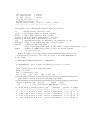
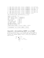
User guide for QSDP-0 – a Matlab software package
for convex quadratic semidefinite programming
Kim-Chuan Toh
∗
February 25, 2010
Working paper
Abstract
This software is designed to solve a convex quadratic semidefinite programming
(QSDP) problem, possibly with a log-determinant term. It employs an infeasible primal-dual predictor-corrector path-following method using the Nesterov-Todd
search direction. The basic code is written in Matlab, but key subroutines in C
are incorporated via Mex interface. It also uses functions in the software for linear
semidefinite programming, SDPT3-3.1. Here we briefly describe how to install and
run QSDP-0. We should emphasize that the current version is an experimental software and it is not intended to be a general purpose solver. Some numerical results
are presented to illustrate the performance of the software on QSDPs arising from the
nearest correlation matrix and the Euclidean distance matrix completion problems.
1
Introduction
n the cone of n × n symLet S n be the space of real n × n symmetric matrices, and S+
metric positive semidefinite matrices. The software package, QSDP-0, is designed to
solve a convex quadratic semidefinite programming (QSDP) problem of the following
form:
o
n1
X • Q(X) + C • X − β log det(X) : A(X) = b, X º 0 ,
(1)
min
X
2
where β ≥ 0 is a given parameter, Q : S n → S n is a given self-adjoint positive
semidefinite linear operator, A : S n → IRm is a linear map, and b ∈ IRm . The
∗
Department of Mathematics, National University of Singapore, Blk S17 (SOC1), 10 Lower Kent Ridge
Road, Singapore 119076 ([email protected]); and Singapore-MIT Alliance, 4 Engineering Drive 3,
Singapore 117576.
1
n . The linear map A can explicitly be written as:
notation X º 0 means that X ∈ S+


A1 • X


..
A(X) = 
,
.
Am • X
m
T
n
where A1 , . . . , Am ∈ S n are given constraint
Pm matrices. Let A : IR → S be the
T
adjoint of A, which is defined by A y = k=1 yk Ak . The Lagrangian dual problem
of (1) is given by:
max
− 21 X • Q(X) + bT y + β log det(Z) + βn(1 − log β)
s.t.
AT (y) − Q(X) + Z = C, Z º 0.
X,y,Z
(2)
Caveats. Our algorithm needs to store the primal iterate X, which is typically
dense. Thus our software may not be able to handle a QSDP with matrix dimension
n ≥ 3000 on an average PC available today. We also assume that the number of
linear constraints m in (1) is less than a few thousands, say m ≤ 5000, so that a
matrix of form A(U ~ V )AT can be computed and stored explicitly. Here U ~ V is
the symmetrized Kronecker product of the symmetric matrices U, V .
It is well-known that (1) can be reformulated into a standard semidefinite-quadraticlinear program (SQLP) by modeling the quadratic term in the objective function by a
second order cone constraint together with q extra linear equality constraints, where
q is the rank of Q. As the resulting SQLP problem has at least m + q linear equality
constraints, and the computational cost of a standard interior-point method for solving such a problem is at least Θ(m + q)3 , it is not difficult to see that reformulating
(1) as an SQLP would be computational undesirable when q = O(n2 ). However,
for n ≤ 100, the SQLP reformulation of (1) can be quite attractive since there are
efficiently and robust interior-point methods for solving a standard SQLP.
There is another form of quadratic SDP given by miny {y T Hy/2 + bT y : AT y ¹
C, y ∈ IRm }, where H is a given positive semidefinite matrix. For this problem, the
Schur complement matrix arising at each interior-point iteration has the form H + M
(with M being the Schur complement matrix associated with the linear SDP without
the quadratic term), and the computation involved at each iteration is very similar to
that for a standard linear SDP. As our interest is in problems with quadratic terms
involving the matrix variables, we shall not consider this form of quadratic SDP in
this software.
For later discussion, we state an example of QSDP arising from estimating the
nearest correlation matrix (NCM) of a given data matrix K ∈ S n :
min
X
n1
2
o
kL(X − K)k2F : diag(X) = e, X º 0 ,
(3)
where e is the vector of ones, and L : S n → S n is a given linear map. By ignoring the
constant term, it is easily seen that (3) can be written in the form (1) with Q = LT L
2
and C = −Q(K). There are two popular choices of Q [7] for the NCM problem:
(a) Q(X) = (H ◦ H) ◦ X corresponding to L(X) = H ◦ X, where H ∈ S n is a
given non-negative matrix and “◦” denotes elementwise product; (b) Q(X) = U XU
corresponding to L(X) = U 1/2 XU 1/2 , where U ∈ S n is a given positive semidefinite
matrix.
Another example of QSDP comes from the Euclidean distance matrix (EDM)
completion problem.
2
Installation
The current version is written in Matlab 7.3. It is available from the internet site:
http://www.math.nus.edu.sg/~mattohkc/qsdp.html
Our software uses a number of Mex routines generated from C programs written
to carry out certain operations that Matlab is not efficient at. To install QSDP-0
and generate these Mex routines, the user can simply follow the steps below:
(a) unzip QSDP-0.zip;
(b) run Matlab in the directory QSDP-0;
(c) run the m-file Installmex.m.
To check whether QSDP-0 has been installed correctly, the user can run the m-files:
>> startup
>> qsdpdemo
3
The algorithm
The algorithm implemented in QSDP-0 is an infeasible primal-dual Mehrotra-type
predictor-corrector path-following algorithm, described in detail in Appendix A. At
each iteration, we first compute a predictor search direction aimed at decreasing the
duality gap by as much as possible. After that, the algorithm generates a Mehrotratype corrector step [9] with the intention of keeping the iterates close to the central path. At each iteration with current iterate (X, y, Z), the predictor direction
(δX, δy, δZ) is computed from the following linear system:
"
#"
#
"
#
−W −1 ~ W −1 − Q AT
δX
Rd − Rc
=
,
(4)
A
0
δy
Rp
δS = Rd − AT δy + Q(δX),
(5)
where W Â 0 is the unique matrix satisfying W ZW = X (W is known as the
Nesterov-Todd scaling matrix), and
Rp = b − A(X), Rd = C − Z − AT y + Q(X), Rc = max{σµ(X, Z), β}X −1 − Z. (6)
3
Here σ ∈ (0, 1) is a centering parameter, and
µ(X, Z) =
1
(X • Z − β log det(XZ) − βn(1 − log β)).
n
(7)
The corrector direction (∆X, ∆y, ∆Z) is also computed from the same linear system
but with Rc in (4) appropriately replaced.
The dimension of the linear system (4) is m + n(n + 1)/2. Typically this system is
too large for solution via a direct solver when n is larger than 100. In this software, we
use a preconditioned symmetric quasi-minimal residual (PSQMR) iterative method
[3] to solve such a system. In [14], three different choices of preconditioners are
designed and analyzed, and their relative performance are described in [14].
3.1
4
Preconditioners used for solving (4)
The main function: qsdp.m
The main routine that corresponds to Algorithm QSDP-IPC described in Appendix
A is qsdp.m, whose calling syntax is as follows:
[obj,X,y,Z,info,runhist] = qsdp(blk,At,C,b,Q,beta,OPTIONS,X0,y0,Z0).
Input arguments.
blk: a cell array describing the block structure of the QSDP problem.
At, C, b, Q: QSDP data.
beta: parameter for the log-determinant term in (1).
If it is not supplied, beta is assumed to be 0.
OPTIONS: a structure array of parameters (optional).
X0, y0, Z0: an initial iterate (optional).
If the input argument OPTIONS is omitted, default values specified in the function
qsdparameters.m are used. More detail on OPTIONS is given in Section 4.1.
Output arguments.
The names chosen for the output arguments explain their contents. Note that X,Z
are cell arrays such that the contents of X{1},Z{1} are approximately optimal primal
and dual solutions, respectively, when the corresponding problems are feasible. The
reason for using cell arrays X,Z to store the matrix variables X, Z is because such a
data structure is more flexible for future extension to QSDP problems with multiple
positive semidefinite matrix variables.
The argument info is a structure array containing performance information such
as
4
info.termcode, info.obj,
info.gap,
info.pinfeas, info.dinfeas, info.cputime
whose meanings are explained in qsdp.m. The argument runhist is a structure
array which records the history of various performance measures during the run; for
example, runhist.gap records the complementarity gap, nµ(X, Z), at each interiorpoint iteration.
Note that, while the output (X, y, Z) normally gives approximately optimal solutions, if info.termcode is 1 the problem is suspected to be primal infeasible and
(0, y, Z) is an approximate certificate of infeasibility, with bT y = 1, Z Â 0, and
kAT y + ZkF small, while if info.termcode is 2 the problem is suspected to be dual
infeasible and X is an approximate certificate of infeasibility, with C •X = −1, X Â 0,
and max{kA(X)k2 , kQ(X)kF } small.
4.1
The structure array OPTIONS for parameters
qsdp.m uses a number of parameters which are specified in a Matlab structure array
called OPTIONS in the m-file qsdparameters.m. If desired, the user can change the
values of these parameters. The meaning of a few of the specified fields in OPTIONS
are given below:
OPTIONS.gaptol
OPTIONS.maxit
OPTIONS.psqmrmaxit
OPTIONS.precond
=
=
=
=
accuracy tolerance
maximum number of interior-point iterations allowed
maximum number of PSQMR steps allowed per linear system
type of preconditioner to use when solving linear system
As an example, if the user wants to solve the QSDP problem to an accuracy tolerance
of 1e-4 instead of the default value of 1e-6 while using the default values for all other
parameters, he only needs to set OPTIONS.gaptol = 1e-4.
4.2
Stopping criteria
At a given iterate (X, y, Z), the algorithm QSDP-IPC is stopped when any of the
following cases occur.
1. solutions with the desired accuracy have been obtained, i.e.,
φ := max {relgap, pinfeas, dinfeas} ≤ OPTIONS.gaptol,
(8)
where
relgap =
pinfeas =
kRp k2
1+kbk2 ,
nµ(X,Z)
1+|pobj|+|dobj| ,
dinfeas =
(9)
kRd kF
1+kCkF
.
(10)
Here, “pobj” and “dobj” denote the primal and dual objective values, and Rp ,
Rd are defined as in (10).
5
2. primal infeasibility is suggested because
bT y/kAT y + ZkF > 108 ;
3. dual infeasibility is suggested because
−C • X/ max{kA(X)k2 , kQ(X)kF } > 108 ;
4. slow progress is detected, measured by a rather complicated set of tests including
relgap < max{pinfeas, dinfeas} ;
5. numerical problems are encountered, such as the iterates not being positive
definite or the Schur complement matrix not being positive definite; or
6. the step sizes fall below 10−6 ;
7. the number of PSQMR steps required to solve the linear system (4) exceeds the
maximum specified in OPTIONS.psqmrmaxit.
5
Coding the problem data
The data structure we adopted for QSDP-0 follows that of the linear SDP software,
SDPT3-3.1.
To be consistent with SDPT3-3.1, the user needs to specify the block structure of
the QSDP problem through the 1 × 2 cell array blk, with
blk{1,1} = ’s’;
blk{1,2} = n;
n and “n” is the dimension. The
where ’s’ indicates that the constraint cone is S+
constraint matrices A1 , . . . , Am are stored in an 1 × m cell array At, where At{1,k}
= Ak , k = 1, . . . , m. The data C ∈ S n is stored in a cell array as C{1} = C, and
b ∈ IRm is stored as the usual Matlab vector. As an example, the data blk, At, b
for the QSDP problem in (3) can be coded as follows:
blk{1,1} = ’s’; blk{1,2} = n;
At = cell(1,n);
for k = 1:n; At{1,k} = spconvert([k,k,1; n,n,0]); end
b = ones(n,1);
The user also needs to specify the linear map Q through a Matlab structure
array Q by setting Q.QXfun to be the name of the Matlab function in which Q(X)
is evaluated given X. Any auxiliary variables needed in Q.QXfun can be stored in
Q. As an example, we consider the QSDP in (3) arising from the nearest correlation
matrix problem with Q(X) = H ◦ X. Suppose the latter is evaluated in the function
QXHadamard.m (supplied in the software) given by
6
function QX = QX_Hadamard(blk,Q,X)
QX = Q.mat{1}.*X{1};
In this case, we set Q.QXfun = ’QX Hadamard’; Q.mat{1} = H. For the linear map
Q(X) = U XU , the user can set Q.QXfun = ’QX SKP’; Q.mat{1} = U .
Important note: the calling syntax for Q.QXfun must have the form as shown in
QX Hadamard.m.
6
Examples
We will now generate some sample runs to illustrate how our package might be used
to solve some test problems. We assume that the current directory is QSDP-0.
>>
>>
>>
>>
startup
%% set up Matlab paths
n=50; m=100;
[blk,At,C,b,Q] = randQSDP(n,m); %% generate a random QSDP
[obj,X,y,Z,info,runhist] = qsdp(blk,At,C,b,Q);
qsdp: converting At into required format
Qnorm = 1.00e+00
num. of constraints = 100
dim. of sdp
var = 50,
num. of sdp blk = 1
************************************************************************
qsdp: Inexact primal-dual path-following algorithms
************************************************************************
version predcorr gam
precond
QXfun
kappa
NT
1
0.000 constrained QXalphaI 1.00e-02
it pstep dstep p_infeas d_infeas gap
mean(obj)
cputime r psqmr
-----------------------------------------------------------------------0 0.000 0.000 1.9e+01 1.5e+01 5.8e+06 1.686322e+06 0:0:00 |%| 5 5
1 0.913 0.913 1.6e+00 1.3e+00 6.1e+05 1.455295e+05 0:0:01 |%| 7 9
2 1.000 1.000 8.2e-12 3.7e-16 1.7e+05 5.217435e+04 0:0:01 |%| 17 16
3 0.917 0.917 1.3e-11 4.1e-16 2.3e+04 3.948290e+04 0:0:02 |%| 33 23
4 1.000 1.000 5.0e-12 4.6e-16 2.9e+03 3.923376e+04 0:0:03 |%| 55 32
5 1.000 1.000 6.4e-13 4.8e-16 1.4e+03 3.905145e+04 0:0:05 |$| 5 5
6 0.972 0.972 1.0e-07 4.6e-16 4.6e+01 3.892347e+04 0:0:05 |$| 5 5
7 0.973 0.973 5.9e-08 4.6e-16 1.7e+00 3.891905e+04 0:0:06 |$| 5 5
8 0.972 0.972 2.4e-08 4.4e-16 5.6e-02 3.891882e+04 0:0:07 |$| 5 5
9 0.967 0.967 9.4e-10 4.7e-16 2.0e-03 3.891881e+04 0:0:07
Stop: max(relative gap, infeasibilities) < 1.00e-06
---------------------------------------------------number of iterations
= 9
primal objective value = 3.89188089e+04
dual
objective value = 3.89188069e+04
gap := trace(XZ)
= 1.96e-03
relative gap
= 5.03e-08
7
actual relative gap
= 5.06e-08
rel. primal infeas
= 9.36e-10
rel. dual
infeas
= 4.65e-16
Total CPU time (secs) = 7.3
CPU time per iteration = 0.8
norm(X),norm(u),norm(S) = 2.06e+02, 1.71e+01, 5.92e+02
----------------------------------------------------
The meaning of the columns in the displayed output are as follows:
it
=
pstep
=
dsetp
=
pinfeas =
dinfeas =
gap
=
mean(obj)
cputime
r
psqmr
interior-point iteration count
step-length taken for primal variable
step-length taken for dual variable
relative primal infeasibility, see (10)
relative dual infeasibility, see (10)
complementarity gap, as defined in the numerator of (9)
= mean of the primal and dual objective values
= cumulative CPU time taken
= type of preconditioner used, or the number of small eigenvalues of Z
= number of PSQMR steps taken to solve the linear systems
at each iteration
In the next example, we generate a sample run for a QSDP arising from the nearest
correlation matrix problem (3). The reader is referred to the m-file NCMexample.m
for the details.
>> NCMexample(’NCM100-Randcorr-1’,’Hadamard’);
0.5*norm(Q(X-B),’fro’)^2 based on simple projection = 2.00e+01
qsdp: converting At into required format
Qnorm = 5.52e+00
num. of constraints = 100
dim. of sdp
var = 100,
num. of sdp blk = 1
************************************************************************
qsdp: Inexact primal-dual path-following algorithms
************************************************************************
version predcorr gam
precond
QXfun
kappa
NT
1
0.000 constrained QXHadamard 1.00e-02
it pstep dstep p_infeas d_infeas gap
mean(obj)
cputime r psqmr
-----------------------------------------------------------------------0 0.000 0.000 6.3e+01 3.1e+01 8.6e+04 -1.594707e+04 0:0:00 |%| 10 7
1 0.964 0.964 2.3e+00 1.1e+00 4.1e+03 -1.093712e+03 0:0:01 |%| 5 6
2 1.000 1.000 9.5e-08 1.3e-16 4.5e+02 -1.509343e+02 0:0:01 |%| 10 9
3 0.971 0.971 5.6e-08 8.0e-17 7.0e+01 -4.971453e+00 0:0:01 |%| 14 13
8
4 0.990 0.990 1.1e-08 7.4e-17 9.7e+00 1.082545e+01
5 0.972 0.972 3.5e-09 7.4e-17 1.1e+00 1.202468e+01
6 0.949 0.949 7.7e-10 7.4e-17 9.0e-02 1.208213e+01
7 0.919 0.919 6.0e-07 8.0e-17 9.7e-03 1.208395e+01
8 0.774 0.774 1.1e-07 7.7e-17 2.2e-03 1.208418e+01
9 0.992 0.992 2.9e-10 8.2e-17 5.2e-04 1.208416e+01
10 0.966 0.966 8.5e-10 8.9e-17 2.0e-05 1.208421e+01
11 0.977 0.977 2.8e-11 8.0e-17 2.1e-06 1.208421e+01
Stop: max(relative gap, infeasibilities) < 1.00e-06
---------------------------------------------------number of iterations
= 11
primal objective value = 1.20842082e+01
dual
objective value = 1.20842061e+01
gap := trace(XZ)
= 2.08e-06
relative gap
= 1.59e-07
actual relative gap
= 1.59e-07
rel. primal infeas
= 2.83e-11
rel. dual
infeas
= 8.02e-17
Total CPU time (secs) = 8.6
CPU time per iteration = 0.8
norm(X),norm(u),norm(S) = 2.11e+01, 7.69e+00, 1.27e+01
---------------------------------------------------0.5*norm(Q(X-B),’fro’)^2 based on QSDP = 1.208e+01
----------------------------------------------------
0:0:02
0:0:03
0:0:05
0:0:05
0:0:06
0:0:07
0:0:08
0:0:09
|%| 29 26
|%|. 107 86
|$| 10 8
|$| 11 9
|$| 13 13
|$| 13 11
|$| 17 14
Appendix: reformulating QSDP as an SQLP
As mentioned in the Introduction, one can reformulate (1) as a standard SQLP, we
show how this is done here. First, factorize Q as Q = RT R. Then hX, Q(X)i ≤ t is
equivalent to the constraints: kR(X)k ≤ s and s2 ≤ t. Hence (1) can equivalently be
written as follows:
minX
1
2t
s.t.
A(X) = b,
+C •X
Xº0
R(X) − z = 0,
s2
≤ t.
9
kzk ≤ s
The standard SQLP reformulation of (1) then becomes:
min
s.t.
1
2t






+C •X


A

R 



0 X + 


0 
0


0
0
0 0
· ¸  0 0
0 −I 
 s


0
0 
 z + 2 0

 0 2
0
0
−1 0
0 0
0
0
0
0
1




 u



 v  + 


 w

0
0
−1
−1
0






t=




b
0
1
−1
0
X º 0, kzk ≤ s, k[v; w]k ≤ u, t ≥ 0.
Here we give a pseudo-code for the algorithm we implemented.
Algorithm QSDP-IPC. Suppose we are given an initial iterate (X 0 , y 0 , Z 0 ) with
X 0 , Z 0 Â 0. Set γ 0 = 0.9.
For k = 0, 1, . . .
(Let the current and the next iterate be (X, y, Z) and (X + , y + , Z + ) respectively.
Also, let the current and the next step-length parameter be denoted by γ and γ +
respectively.)
• Compute µ(X, Z) as in (7).
• (Convergence test)
Stop the iteration if the accuracy measure φ defined in (8) is sufficiently small.
• (Predictor step)
Compute the predictor direction (δX, δy, δZ) from (4)–(5) by choosing σ = 0 in
Rc .
• (Predictor step-length)
Compute
(12)
Here α is the maximum step length that can be taken so that X + αδX and
Z + αδZ remain positive semidefinite.
• (Centering parameter)
Set σ = µ(X + αp δX, Z + αp δZ)/µ(X, Z).
• (Corrector step)
Compute the correct direction (∆X, ∆y, ∆Z) from (4)–(5), with Rc in (4) appropriately replaced.
10





(11)
Appendix: An infeasible primal-dual interiorpoint algorithm
αp = min (1, τ α) .

• (Corrector step-length)
Compute αc as in (12) but with (δX, δZ) replaced by (∆X, ∆Z).
• Update (X, y, Z) to (X + , y + , Z + ) by
X + = X + αc ∆X,
y + = y + αc ∆y,
Z + = Z + αc ∆Z.
(13)
• Update the step-length parameter by τ + = 0.9 + 0.08αc .
References
[1] P. Apkarian, D. Noll, J.-P. Thevenet, and H. D. Tuan, A spectral quadratic-SDP
method with applications to fixed-order H2 and H∞ synthesis, Research Report,
Universite Paul Sabaitier, Toulouse, France, 2004.
[2] B. Borchers, SDPLIB 1.2, a library of semidefinite programming test problems,
Optimization Methods and Software, 11 & 12 (1999), pp. 683–690. Available at
http://www.nmt.edu/~borchers/sdplib.html.
[3] R.W. Freund and N.M. Nachtigal, A new Krylov-subspace method for symmetric
indefinite linear systems, Proceedings of the 14th IMACS World Congress on
Computational and Applied Mathematics, Atlanta, USA, W.F. Ames ed., July
1994, pp. 1253–1256.
[4] K. Fujisawa, M. Kojima, K. Nakata, and M. Yamashita, SDPA (SemiDefinite
Programming Algorithm) User’s manual — version 6.2.0, Research Report B308, Department Mathematical and Computing Sciences, Tokyo Institute of
Technology, December 1995, revised September 2004.
[5] K. Fujisawa, M. Kojima, and K. Nakata, Exploiting sparsity in primal-dual
interior-point method for semidefinite programming, Mathematical Programming, 79 (1997), pp. 235–253.
[6] G.H. Golub and C.F. Van Loan, Matrix Computations, 2nd ed., Johns Hopkins
University Press, Baltimore, MD, 1989.
[7] N.J. Higham, Computing the nearest correlation matrix — a problem from finance. IMA J. Numerical Analysis, 22 (2002), pp. 329–343.
[8] M. Kojima, S. Shindoh, and S. Hara, Interior-point methods for the monotone
linear complementarity problem in symmetric matrices, SIAM J. Optimization,
7 (1997), pp. 86–125.
[9] S. Mehrotra, On the implementation of a primal-dual interior point method,
SIAM J. Optimization, 2 (1992), pp. 575–601.
[10] M.J. Todd, K.C. Toh, and R.H. T¨
ut¨
unc¨
u, On the Nesterov-Todd direction in
semidefinite programming, SIAM J. Optimization, 8 (1998), pp. 769–796.
[11] K.C. Toh, M.J. Todd, and R.H. T¨
ut¨
unc¨
u, SDPT3 — a Matlab software package for semidefinite programming, Optimization Methods and Software, 11/12
(1999), pp. 545-581.
11
[12] R.H. T¨
ut¨
unc¨
u, K.C. Toh, and M.J. Todd, Solving semidefinite-quadratic-linear
programs using SDPT3, Mathematical Programming Ser. B, 95 (2003), pp. 189–
217.
[13] K.C. Toh, R.H. T¨
ut¨
unc¨
u, and M.J. Todd, Inexact primal-dual path-following
algorithms for a special class of convex quadratic SDP and related problems.
Pacific J. Optimization, 3 (2007), pp. 135–164
[14] K.C. Toh, An inexact primal-dual path-following algorithm for convex quadratic
SDP, Mathematical Programming, 112 (2007), pp. 221–254.
12