Download USER'S GUIDE to PROGRAM DBWS-9807a RIETVELD

DBWS-9807a User's Guide
17.5.99
USER'S GUIDE
to
PROGRAM DBWS-9807a
for
RIETVELD ANALYSIS OF X-RAY AND NEUTRON
POWDER DIFFRACTION PATTERNS
with a `PC' and various other computers
R. A. Young, Allen C. Larson1 and C.O. Paiva-Santos2
School of Physics
Georgia Institute of Technology
Atlanta, GA 30332
(17.5.99)
20.8.00
Copyright notice:
© 1998, 1999,2000 R. A. Young
All rights reserved
Current Addresses:
1) Dr. Allen C. Larson, 14 Cerrado Loop, Santa Fe, NM 87505-8248
2) Prof. C. O. Paiva Santos, Instituto de Quimica - UNESP, C.P. 355, 14800-900 Araraquara, SP,
BRAZIL
DBWS-9807a User's Guide
20.8.00
CONTENTS OF THIS GUIDE
Item
Page
Part 1. Preliminaries
I. Foreword A. History of DBWS
B. What is new in the 9807 version
4
5
II. Platforms and Environments
A. Portability
B. Windows environment
8
III. Contents of the Distribution Package
9
Part 2. The refinement programs
I. General information
A. General plan and data types accommodated
B. Calculated intensities
C. Selectable models
1. Profile shape models (functions)
2. Preferred orientation models
3. Profile asymmetry models
4. Background representation - four types
5. Models for surface roughness effects
D. Quantitative phase analysis
1. Procedure
a) With no internal standard
b) With an internal standard
2. Microabsorption
E. Codewords and constraints
F. Array size selection and executable program size
II. Description of input files
A. The Input Control File (ICF)
1. What it is and how to create and update it
2. Line by line instructions
3. Example
2
11
12
13
17
17
18
18
19
20
20
21
22
24
25-35
36
DBWS-9807a User's Guide
20.8.00
B. The observed data files
Category 1: Constant incident flux and a single detector
(7 data formats accepted)
Category 2: Varying incident x-ray flux (e.g., synchrotron) and
a single detector
Category 3. Fixed wavelength and multiple detectors
(e.g., CW neutron sources)
C. Background data files
1. 'Tape 3'
2. 'Tape 11'
III. Description of output files
A. Plot files
1. PLOTINFO file for general use
2. PLOT FILES when NBCKGD = -1
B. Updated Input Control File
C. Output to terminal during run
D. The main output file
1. Standard parts of the main output file
2. Optional outputs to this and other files
E. Definitions and interpretations of the numerical criteria of fit,
1. e.s.d.'s, R's, GofF, DW-d
2. Comment about interpretation of R's
Part 3. Further comments on using DBWS-9411 and 9807 with a PC
A. Compiling
B. Plots
1. Production and chacteristics
2. Use - An adroit example
C. Execution procedure
1. In DOS
2. Using DBWS in Windows
37
39
40
40
40
42
42
43
43
44
44
45
46
48
48
49
50
51
REFERENCES
54
APPENDICES
A. Other programs
1. Other Rietveld refinement programs
2. Programs ancillary to DBWS
a) ICF preparation programs
56
57
3
DBWS-9807a User's Guide
20.8.00
b) DB2dI assembly program
B. Copyright and Fair Use
57
59
FIGURES
60 - 74
PART 1. Preliminaries
I. FOREWORD - History of DBWS and what is new in this version
A. History
The program is designed to carry out Rietveld refinements with X-ray or neutron powder diffraction
data in digitized form collected under any of several of the most commonly used instrumental conditions.
Fixed wavelength(s) and equal increments in the scattering angle, 2?, are required conditions.
The current program is the latest in a long chain of versions, each updated and upgraded from its
predecessor and each distributed in a `distribution package' containing the source code, a User's Guide,
plus data and Input Control Files for test cases. For the 1990 (the date of the first PC version) and later
distributions, executable versions of PC-compatible (MSDOS) plot programs were included. These plot
programs were offered by third parties as Shareware items.
The chain started with DBW2.9 (Young and Wiles, 1981) which was written in FORTRAN IV and
incorporated some parts of Rietveld's (1969) original code, particularly the codeword system, A. W.
Hewat's code for anisotropic thermal parameters, and A. C. Larson's code for dealing with space group
symmetries and reflection multiplicities. However, it was otherwise written `from scratch' and incorporated
many new features, some quite major. It was written to be used with x-ray as well as neutron data, to be
modular, single pass, and portable. Some of the other new features were choice of a variety of profile
functions, a refinable background model, a multiple phase capability, and a number of other features listed
in Wiles and Young (1981). DBW2.9 (which, incidentally, had several `bugs') was soon followed by
DBW 3.2 (1982) written in FORTRAN V. DBW3.2 was superseded in 1987 by DBW3.2S, a rather
major revision made by A. Sakthivel and more nearly conforming to ANSI 77 standards. Next followed
versions DBWS-8711 (November, 1987) and, in turn, DBWS-8804 (April 1988). Version
DBWS-8804 had a small bug which allowed only 2 phases, rather than the intended 8, to be refined
correctly. That error was corrected in version DBWS-8804a. In the next major modification, the program
was adapted to run on PC-type computers and was named DBWS-9006PC. This version, with the
CalComp instruction routine omitted, was fully ANSI77. Subsequently, various of the several hundred
users of record have successfully compiled and run DBWS-9006 on a variety of computers, both small
and large. The principal differences between successive versions, up to this point, were listed in the
appendices to the relevant versions of the User's Guide and, for the DBWS-8804 to DBWS-9006
differences, in the Foreword of the User's Guide for DBWS-9006.
The principal differences between the next version, DBWS-9411, and DBWS-9006 were (1)
4
DBWS-9807a User's Guide
20.8.00
rearrangement of the input control file (ICF) to make it more user-friendly, (2) correction of the
long-standing error (noted in the earlier User's Guides) of a factor of two in the multiplicities calculated for
some Laue groups, (3) addition of four surface-roughness models with refinable parameters, (4) addition
of a split Pearson VII profile function to provide another means of modeling (still imperfectly) profile
asymmetry, (5) addition of a quantitative phase analysis routine (see comments below), (6) an improved
method for inputting the selectable sizes of certain arrays at compilation time (via a `param.inc' file) plus
readout of those sizes to screen during and to output file after each refinement, (7) addition of a dynamic
screen display of the progress of the current refinement cycle, (8) additions to the output to the plotting file
PLOTINFO and addition of PLOTINFO.BIN so that the plotting program DMPLOT can display the
Miller indices at each reflection location and can display (simultaneously) the separate calculated patterns
for each of the various phases being refined in a multiphase specimen, (9) change of the Durbin-Watson
statistic, d, to the mathematically preferred unweighted version, and (10) some additional diagnostics.
We are indebted to Dr. H. Marciniak (author of DMPLOT) for providing features 6, 7 and 8, above.
The split Pearson VII code is based on the mathematics actually used by Toraya for this function in
his program PRO-FIT introduced in Toraya (1986).
The quantitative phase analysis calculation, provided by Paiva-Santos, uses the formulation of Hill
and Howard (1987) to produce the phase fraction, by weight, that each modelled phase constitutes of the
total weight of the modelled phases. The calculation is based on the refined values of the scale factors,
lattice parameters, and atom-site occupancies as updated in each least-squares cycle plus the
incorporated table of atomic weights. The atomic-weights table covers all atoms for which scattering
factors are included in their incorporated table. If other atoms are used, their atomic weights must be
supplied by the user in line 8.1 of the ICF (Input Control File; see §IIA). If the mol fraction is also wanted,
the number of formula units per cell must be provided by the user. It is important to note that in the version
9411 form the phase-fraction calculation is made WITHOUT any correction for microabsorption. In
x-ray work, especially, that can be a serious problem requiring separate analysis. But see (9), below and
§II1D2.
B. What is new in the 9807 and 9807a versions
The changes from version 9411 made to produce the current version, 9807, include the following.
(Listed in arbitrary order.)
1) The format of the ICF (Input Control File) has been changed, particularly with respect to
atom-site multiplicity and site occupation number. In the ICF for the 9411 version, the parameter N for
the 'site occupancy multiplier' for an atom was in the last position in the first of the four lines for the atom.
In the 9807 (the current) version, N has been replaced by the actual, refinable site occupancy, 'So', in
the last position and the actual site multiplicity, M, (not refinable) is called for in the newly created third
position. The user must supply M. It is always an integer value which depends on the particular space
group and Wyckoff site. The values of M for all space groups and Wyckoff sites are given in the
5
DBWS-9807a User's Guide
20.8.00
International Tables for Crystallography. They can also be found in the Inorganic Crystal Structure
Database for many of those materials for which the crystal structures are included. They can also be
deduced from the atom's coordinates and the full set of symmetry operations for the space group. Setting
flag 9 in line 3 of the ICF will cause the full set of symmetry operators to be printed out. Categories 2 and
3 remain unchanged.
2) A subroutine for converting the format of an ICF for the 9411 version to the format for the 9807
version is provided. It is called up by setting NPROF, the profile function identifier in the second position
of line 2 of the ICF, to any single integer value <0. Runnning the program as though one were doing a cycle
of least squares then produces the converted ICF under the name specified as the output file in the
command line. The user has then to fill in correct values for M, So and other parameters, if any, not
present in the 9411 version. As a further aid to the user, the multiplicity of the general site (for the space
group involved) is printed in the first part of the main output file, on the line between the first mention of the
space group and the listing of the initial parameters.
3) The variety of data formats accepted by DBWS in Category 1 (See § 2.II.B) has been increased
to include, in addition to the ‘standard DBWS format, a free format, the GSAS 'standard' format, Philips
UDF format, a Scintag text format, a Siemens UXD format, and a Rigaku ASCII format. All of the
additions are based on equal steps in 2?, a single detector, and constant incident beam intensity.
4) The output of structure-factor magnitudes, called for by flag 3 in line 3 of the ICF, can now be
called to report the structures factor phases, as well.
Setting the flag at '2' calls for the phase angles to be reported, as such, for use in
FK = |FK| exp (i f K)
where f K is the phase angle and i is the square root of (-1).
Setting the flag at '3' calls for this output to include phase angle information by reporting F in the A
+ iB form.
In the process of making these changes to the structure factor outputs, an earlier error was corrected
so that the |F|'s are now reported to 3 decimal places and do not differ for the a1 and a2 wavelengths.
5) The number of phases that can be handled at once has been increased from 8 to 15. The main rational
for this increase is to accommodate quantitative phase analyses which can benefit from inclusion of many
phases for which the structure is known and only the scale factor and one or two other parameters need
to be refined. Dr. Marciniak's DMPLOT also handles 15 phases now.
6)* The quantitative phase analysis routines have now been extended to include an option for operation
6
DBWS-9807a User's Guide
20.8.00
directly with an internal standard.
7)* A calculation of the wt% of the ‘amorphous’ component is now offered when an internal standard
is used.
8) X-ray anomalous dispersion coefficients for the atoms have been added for 5 more wavelengths,
bringing the total to 10 sampling the wavelength range from 2.75 to 0.18 A. We are grateful to Ian
Madsen and Dr. R. J. Hill of CSIRO Minerals (Australia) for providing the values and associated coding
for these coefficients.
9) The preferred orientation correction now works correctly for high-symmetry, non-unique axis cases
as well as the others. The existence of the now-fixed problem and conditions under which it might have had
significant effects were pointed out in the User's Guide to the 9411 version.
10) FWHM. As recommended by the ICDD (Lowe-Ma, et al, 1997) and by Cheary and Cline (1994),
a term in cot2? has been added to the 'Caglioti' (Caglioti, et al. 1958) expression for the FWHM (Full
Width at Half Maximum) in profile functions 0,1,2,3,5 and 6, i.e., for the Gaussian, Lorentzian, simple
pseudo-Voigt and symmetric Pearson VII functions.
11) A tentative model for microabsorption effects (relevant to quantitative phase analysis) has been
provided for testing and user suggestions for improvements.
12) Much of the source code, primarily that relating to space groups and symmetry operations and
multiplicities, has been 'cleaned' in the sense of improved readability, consistency in formatting and in use
of variable names (e.g., floating point and integer arrays can not use the same name even though used in
different places), and removal of unused code.
-----------------------------------------------------------------------------------------------------------------Additions 13 through 17, below, have been made at the suggestion of Fagherazzi's group in Italy, who
made these and other additions to their copy of DBWS-9006 (Riello, Canton, and Fagherazzi, 1995;
Riello, Fagherazzi, et al., 1995). We thank them for kindly supplying their code for us to work with.
13) An alternative model for profile asymmetry has been added.
14) Code has been added for calculation of the background contributions of Compton scattering and
disorder-diffuse scattering. This is a part of their (Riello, et al.) 'physically based background'.
15) An intensity correction for transmissivity (low absorption) has been added which may be useful for
a flat-plate sample mounted in forward transmission geometry.
7
DBWS-9807a User's Guide
20.8.00
16) A model data set for some component of the sample may now be imported (Tape 11) and have its
scale factor refined along with the parameters related to the main data set and the instrument. Reillo, et al.
developed this feature to model an amorphous component of the background with a pattern of an
amorphous material stored on Tape 11. The possibility is being explored that this scheme may work for
a crystalline component for which the diffraction pattern is known but not the structural data needed for
regular Rietveld refinement. In version 9807, a modest step has been taken to deal with this problem.
17) Plots can be made of the separate contributions to the background (e.g,, Compton and disorder) as
well as the entire modeled background.
________________________________________________
*New in version 9807a.
II. Platforms and Environments
A. Portability
The source code provided can be used to carry out Rietveld refinements on various mainframes,
workstations, and PC's as well as MacIntosh personal computers. The user must comment out the parts
not applicable to the platform at hand. For example, it might be necessary to verify that the
bitwise-mapped logic statements AND, OR and XOR are properly recast in all occurrences. The
DBWS source code now provided is fully ANSI 77 as passed by Microsoft FORTRAN PowerStation
1.0a.
The executable code provided for DBWS is DOS-executable, but can be run rather advantageously
in the Windows-95/98 environment. (See §IIB, below.)
Only executable code is provided for the Shareware plotting program included in the distribution
package for making the plots of the Rietveld results (see Note 3, below). The DBWS program does
output two files which can be used for plotting, PLOTINFO and PLOTINFO.BIN. PLOTINFO can
probably be used by a number of plotting programs including the formerly distributed Shareware program
SPLOT by Sakthivel and the presently distributed Shareware program DMPLOT (DMPLOT3.48 as of
this writing) by Diduszko and Marciniak. PLOTINFO.BIN is a binary file tailored specifically for the
program DMPLOT which, then, can display the Miller indices and the patterns of the separate phases,
as noted above. The plots can be produced on-screen and dumped to a printer or produced directly on
a plotter.
B. Windows environment
Although they are DOS programs, the executables provided for DBWS can run in the Windows 95
8
DBWS-9807a User's Guide
20.8.00
(also 98 and NT) environments in a DOS window automatically called up when the program execution
starts. Advantage can thereby be taken of some of the 'drag and drop' and file handling conveniences of
Windows 95/98/NT. In combination with a windows-based file editor that does not leave ‘tracks’ (i.e.,
control characters, etc.) incompatible with program, the convenience and ease of operation under
Windows can be equal to that to be expected if DBWS were written as a Windows based program.
Further, detailed information about how to achieve this convenience and ease is given in Part 3, §C3.
III.
CONTENTS OF THE DISTRIBUTION PACKAGE
The files in the distribution package for DBWS-9807a are generally provided on two 3-1/2 inch 1.44
MB diskettes written under MSDOS. Distribution on other media can be arranged on special request.
The distribution package consists of this User's Guide plus the following files on magnetic media in
six subdirectories, all written under MSDOS.
1. In subdirectory FOR:
DBWS-9807a.FOR (the DBWS source code)
PARAM.INC
DOSXMSF.EXE
The file, PARAM.INC, is needed at compilation time. It conveys the user's choice of the sizes for the
five most-likely-to-be-redimensioned arrays.
DOSXMSF.EXE must be either in the path or in the same directory with the executable version of
DBWS that is running.
2. In subdirectory FTEST: files for a test case with fluorapatite. This is a single phase case with a moderate
quantity of “lines” (Bragg reflection profiles).
FDATA - the observed-data file
FIN - the ICF (set up for refining 31 parameters) as rewritten after the last cycle run.
PLFAP - the PLOTINFO file needed by SPLOT and DMPLOT, renamed for saving
PLFAP.BIN - the binary file needed by DMPLOT to display the Miller indices and the
calculated patterns for the separate phases.
FOUT - the main output file from a run based on FIN
README - Comments about this example.
3. In subdirectory QTEST: files for a two phase case of quartz with alumina as a minor impurity:
9
DBWS-9807a User's Guide
20.8.00
QOUT - the main output file from a run based on QIN
PLQ - the PLOTINFO file, renamed for saving, needed by DMPLOT.
PLQ.BIN - the binary file needed by DMPLOT to display the indices and separate phase
patterns
QDATA - the observed-data file
QIN - the Input Control File (ICF) as rewritten at the end of the last cycle.
4. In the subdirectory QPATEST you find the files for a somewhat more advanced case involving
quantitative phase analysis: 3 phases, one of which is the internal standard, plus an amorphous component.
To be determined are the wt% present of two phases plus the amorphous component.
QPADATA - the observed data (3 crystalline phases plus an amorphous component)
QPA .IN - the input control file (ICF)
QPA.OUT
‘TAPE11" - whole-pattern observed data for an amorphous silica sample
PLQPA - thePLOTINFO file for this case (note how well the amorphous component is fit)
PLQPA.BIN
5. In subdirectory DMPLOT: files for using this proprietary program offered as a SHAREWARE item:
DMPLOT.CFG - Configuration for DMPLOT
DMPLOT.EXE (Version 3.48)
DMPLOT.TXT - Notes on DMPLOT
6. In the subdirectory XCUTABLE there are three DOS-executable versions of DBWS-9807. They
differ only in the choices of dimensions of the five arrays listed in PARAM.INC. See the accompanying
Read.me file for details.
7. The current distribution program includes another diskette with a PC-executable program named
DB2dI provided by the International Center for Diffraction Data (ICDD). The ICDD hope you will use
it to provide good patterns properly formatted for acceptance in their PDF (Powder Diffraction File.) See
§2b of Appendix A (p. 54) for further information about this program.
NOTES
1) Some of the test-case data files are rather long (e.g., 20 - 140 °2? in 0.02° steps). You may wish to
use only a portion of each, e.g., 20 - 60°, to save computer time when you are making your first trial runs.
See the discussion (Part 2, §II B) of the data file to find how to do this.
2) At the beginning of refinement with a new data set, it is advantageous to refine just a few parameters
at first, then those plus a few more, etc. It is, therefore, advantageous to assign the lowest-numbered
codewords to those first-to-be-refined parameters. The choice of codeword sequence in the Input
Control Files (Part 2, §IIA) for these test-cases has been influenced (but not fully controlled) by that
10
DBWS-9807a User's Guide
20.8.00
thought.
PART 2. The Rietveld refinement program
I. General Information
A. General plan and data types accommodated
This program is designed to perform Rietveld (1967, 1969) analysis on x-ray or neutron
(nuclear scattering, only) powder diffraction data collected:
(i) with a fixed-slits ? - 2? diffractometer (`Bragg-Brentano' geometry) operated in a step-scan
mode (equal steps in 2?) with a single detector and with either one or two (e.g., a-doublet) wavelengths
in the constant intensity incident x-ray beam (Data in this category are now accepted in six specific formats
and a free format.)
(ii) as for (i) but with a varying incident x-ray beam intensity as from a synchrotron source, or
(iii) with fixed incident neutron-beam intensity (or monitor count) and wavelength and with multiple
counters which do not all contribute at every step, such as the HRNPD instrument at Brookhaven National
Laboratory (USA) and the D1A and D2B instruments at ILL (France).
It can also be used with data collected in HDS geometry from non-absorbing specimens.
It can be used with other geometries if an external data-preparation step is taken, e.g. to compensate
for the differences, e.g., the effects of a varying divergence slit or the angle-dependent absorption in
absorbing specimens used in HDS or Guinier geometry.
The program can also be used in a pattern calculation, only, mode.
The program is currently set up to handle up to fifteen phases simultaneously. The previously used
number, eight, was chosen on the presumption that most powder diffraction patterns are not likely to have
enough information in them to support refinement of structural details in more than eight phases at once.
However, there is now widespread and growing recognition that multiphase Rietveld refinement is the
very best way to do quantitative phase analysis (QPA) if the structures are known or are known well
enough to be refined. Therefore cases will occur commonly, in quantitative phase analysis, in which only
a few parameters, often only the scale factor, need be refined for most of the phases. In such cases,
sensible QA results can be expected for many more than 8 phases with good data. Even the 15 now
accommodated may not always be enough.
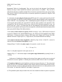
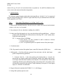
The program uses the Newton-Raphson algorithm to minimize the quantity:
11
DBWS-9807a User's Guide
20.8.00
Sy = S wi(yi - yci)2
where
wi = 1/yi,
yi = observed (gross) intensity at the ith step,
yci = calculated intensity at the ith step,
and the sum is over all data points.
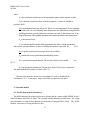
The normal matrix elements formally given by
∂2yci
∂yci ∂yci
Mjk = -Si 2wi[(yi-yci) --- - (---) (--)] ,
∂?j ∂?k ∂?j ∂?k
(where the ?k are the adjustable parameters) are approximated by deletion of the
∂2yci
(yi - yci)--- term.
∂?j∂?k
Parameters are stored internally in arrays XL(I,J), GLB(I), and PAR(I,J). XL contains the data for
the atoms. The first index runs over the atoms; the second over the parameters for the atom. GLB
contains `global' parameters, those which apply to all phases, such as surface roughness, 2?-zero,
specimen displacement, background and others. PAR contains crystalline-phase dependent parameters
such as lattice constants, scale factor, profile shape parameters ? and m, and preferred orientation
parameters. The first index runs over the phases. There are corresponding arrays LP, LGLB, and LPAR
which map the parameters to the normal matrix elements. This mapping is determined by the user through
the use of `codewords'. See §ID, below.
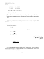
B. Calculated intensities
The calculated counts yci are determined by summing the contributions from neighboring Bragg
reflections, K, for all phases, p, plus the background, bi:
yci = SR[Σ p sp Ab [SK [FK2 F(2? i - 2? K) As LK PK]]p + ybi]
12
DBWS-9807a User's Guide
20.8.00
where
sp is the scale factor for phase p (note that quantitative phase analysis depends on this),
SR is a function to model the effects of surface roughness. A choice of 4 models is
provided (§IC4).
Ab is an absorption factor, here left at 1.00. That is, it is not implemented. That is acceptable
for (1) the x-ray case of an "infinitely" thick flat specimen in a diffractometer using fixed slits
and Bragg-Brentano geometry (the most common case) and (2) the neutron case of any
shape of specimen with negligible absorption and completely bathed in the neutron beam.
FK is the structure factor,
F is a reflection profile function which approximates the effects of both instrumental
and, possibly, specimen features. A choice of 8 analytical functions is provided. See
§I.C.1.
As is a profile asymmetry function (two choices are available)
LK contains the Lorentz, polarization and multiplicity factors,
PK is a preferred orientation function. The user has a choice of two models.
See
§I.C.2.
bi is the background contribution. The user has a choice of four ways to represent it.
The fourth method has a number of subsets. (2§I.C.4).
The ratio of the intensities for the two a wavelengths (if used) is absorbed in the
calculation of FK2, so that only a single scale factor is required for each phase.
C. Selectable models
C.1. Profile shape models (functions), F .
The profile function to be used in a given run is selected with the control variable NPROF in line 2
of the ICF (Input Control File, see §IIA). The currently available functions are listed below. The origins
and performances of most of these functions are discussed in Young and Wiles (1982). The TCHZ
function is discussed in Young and Desai (1989).
13
DBWS-9807a User's Guide
20.8.00
NPROF
FUNCTION
NAME
0) √Co exp(-Co (2? i -2? K)2 /HK2 )
HK√p
Gaussian (`G')
1) √C1
p HK
Lorentzian (`L')
1/[1+C1(2? i -2? K)2/HK2]
2) 2 √C2 1/[1+C2(2? i-2? K)2/HK2]2
p HK
Mod 1 Lorentzian
3) √C3_ 1/[1+C3(2? i-2? K)2/HK2]3/2}
2 HK
Mod 2 Lorentzian
4) Split Pearson VII
(`SPVII)
Low-angle side, Split Pearson VII
C 4 [1+ (
(`SPVII-L')
1 + A 2 1/ mL
2 ) ( 2 - 1) (2 θ i - 2θ K ) ] mL
A
High-angle side, Split Pearson VII
(`SPVII-H')
2
2 -m
1/
C 4 [1+ (1 + A ) ( 2 mH - 1) (2 θ i - 2 θ K ) ] H
`A' in this function is a refinable asymmetry parameter. The shape parameters mL and mH can
be refined individually as a function of 2? in the same way as can m in the single PVII, profile function 6.
These formulations of the normalized SPVII functions are taken from Toraya (1986).
14
DBWS-9807a User's Guide
20.8.00
5) ?L + (1-?)G
pseudo-Voigt (`pV')
The mixing parameter, ?, can be refined as a linear function of 2? wherein the refinable variables
are NA and NB:
? = NA + NB*2?
Hastings, et al. (1984) have shown how the FWHM's of the individual L and G components can be
recovered from the ? values in this profile function.
6) (C 5/HK) [1 + 4(21/m - 1)(2? i - 2? i)2/HK2]
Pearson VII (`PVII')
and m can be refined as a function of 2? as
m = NA + NB/2? + NC/(2?)2 ,
where the refinable variables are NA, NB, and NC.
We note that PVII = L if m = 1 and G if m = ∞.
7) Modified* Thompson-Cox-Hastings pseudo-Voigt
(Thompson, et al., 1987)
Mod-TCH pV (`TCHZ')
[Note: The G used in the description of this function is simply a symbol related to the profile
breadth and is not to be confused with the gamma function represented by G(m) in the definition of the
normalizing constants, C4 and C5, in the PVII functions.]
TCHZ = ?L + (1-?)G
where
? = 1.36603q - 0.47719q2 + 0.1116q3
q = GL/G
G = (GG5 + AGG4GL + BGG3GL2 + CGG2GL3 + DGGGL4 + GL5)0.2 = HK
15
DBWS-9807a User's Guide
20.8.00
A = 2.69269
C = 4.47163
B = 2.42843
D = 0.07842
GG = (U tan2? + V tan ? + W + Z/cos2?)1/2
GL = X tan ? + Y/cos ?
[*The modification consists of addition the parameter Z to provide a component of the Gaussian
FWHM which is constant in d*, as is the Y component of the Lorentzian FWHM (Young and Desai,
1989)]
In the above profile functions, the refinable parameters are those in ?, m, HK and (in the SPVII
functions) A.
The normalizing constants are
Co = 4 ln2
C1 = 4
C 2 = 4( 2 - 1 )
C 3 = 4( 2 2/3 - 1)
C4 =
C5 =
2 (1+ A)
[
π HK
2 Γ(m)( 21/m - 1 )1/2
π Γ(m - 0.5)
HK is the full-width-at-half-maximum (FWHM) of the Kth Bragg reflection. Except as otherwise
specified (e.g., in Profile 7), the angular dependence of HK is modeled in accord with the ICDD
recommendation (Lowe-Ma et al., 1997) as
16
A Γ( mL
21/ mL - 1
DBWS-9807a User's Guide
20.8.00
HK2 = U tan 2? + V tan ? + W + CT cot2 ?
where U, V, W and CT are refinable parameters.
C.2. Preferred orientation (PK) models
In position 8 of line 2 in the ICF, a 0 selects the Rietveld-Toraya model and a 1 selects the
March-Dollase model. The Rietveld-Toraya model, Toraya's modification of the function Rietveld put in
his original code, is
PK = [G2 + (1-G2) exp(G1a K2)]
and the March-Dollase model is
PK = (G12 cos2a + (1/G1) sin2a)-3/2),
where G1 and G2 are refinable parameters and a K is the angle between d*K and the presumed
cylindrical-symmetry axis of the texture (e.g., fiber axis direction). We note that the value of G1
corresponding to no preferred orientation is 0 in the Rietveld-Toraya function and 1.00 in the
March-Dollase function.
It may be noted here that in the Rietveld-Toraya model, the G1 parameter tends to be correlated with
the scale factor, Sp, highly so if the preferred orientation is strong.
C. 3. Profile asymmetry models
Two choices are available:
Setting flag 9 in ICF line 2 to 0 selects the "usual Rietveld asymmetry model":
As = 1-P*sign(2? i-2? K)*(2? i-2? K)2/tan? K
Setting that flag to 1 selects the Riello, Canton and Fagherazzi (1995) model
(2θ - 2 θ K )
| 2θ - 2 θ K |
As(2θ - 2θ K ) = 1+ C M
exp()
2 wK
wK ( tan θ K )
17
DBWS-9807a User's Guide
20.8.00
where CM is the refinable parameter, 2? K is the position of the peak of the Kth reflection profile, (2? 2? K) is the displacement of the observed peak from the calculated one` and wK is the refined value of the
FWHM of the Kth reflection.
C.4. Background representation
The background intensity ybi at the ith step may be obtained by any of several methods. The user's
choice is indicated by the value of NBCKGD entered in the fourth position in line 2 of the ICF. The
choices are
(1) an operator-supplied table (‘Tape 3') of background intensities (NBCKGD = 1), or
(2) linear interpolation between operator-selected points in the pattern
(NBCKGD = n, where n is the number of points), or
(3) a specified background function (NBCKGD = 0) or
(4) the alternative background representation of Reillo, et al (NBCKGD = -1)
If the background is to be refined in the NBCKGD = 0 option, ybi must be obtained from a refinable
background function. The one available in the current version of DBWS is
5
ybi = S Bm [(2? i/BKPOS)-1]m.
m=0
where BKPOS is user-specified in line 4 of the Input Control File (ICF). See §IIA.
If the alternative background (NBCKGD = -1) is to be used, there are several choices to be made.
(1) Absorption correction for Bragg-Brentano geometry
(2) Compton and disorder diffuse scattering contribution for each phase using either individual isotropic
or overall atom-displacement factors.
(3) Refinement of the scale factor for an ‘amorphous’ (or other?) component represented by
whole-pattern intensity data on Tape 11.
C.5. Models for Surface Roughness effects (SR)
As was dramatically demonstrated by Sparks, et al. (1992), surface roughness has a far more
important effect on the relative intensities than had been generally appreciated. Here we offer the user a
choice among four models in the spirit of experimentation: no guarantees that any of them are particularly
18
DBWS-9807a User's Guide
20.8.00
appropriate. Their refinable parameters are likely to be highly correlated with each other and, of course,
with the overall scale factor. However, they do represent a gesture in the right direction. We would be
grateful to learn of your experiences in using one or more of these options.
The user's choice among the 4 different models is indicated by the digit entered for IABSR in line 2
of the ICF.
The choices of model are:
IABSR
Model
1
Combination of the Sparks and Suortti models
2
Sparks, et al., (1992) model (straight line)
3
Suortti (1972) model (exponential)
4
Pitschke, et al., (1993) model
The models, as recast and normalized to 1.00 at ? = 90° by us, are:
1 - Combination model:
SR = r{1.0 - p(exp[-q]) + p(exp[-q/sin(?)])} + (1-r)(1+t(?-p/2))
2 - Sparks, et al., model:
SR = 1.0 - t(?-p/2) [? in radians]
3 - Suortti, et al., model:
SR = 1.0 - p(exp[-q]) + p(exp[-q/sin(?)]
4 - Pitschke, et al., model:
SR = 1.0 - [pq(1.0-q)] - [pq/sin(?)][1.0-q/sin(?)]
The refinable parameters are p,q,r, and t. Note that ? is expressed in radians.
If no correction is being applied for surface roughness effects, then set (and fix) p = q = 0 and r = 1.0 if
IABSR = 1 and p = q = r = t = 0 for all other choices of IABSR (2,3,4). In the Pitschke, et al. model,
q must not be 0 (zero) if a codeword is declared for it, else a `divide by zero' error message will appear.
D. Quantitative phase analysis
1. Procedure.
a) No internal standard
19
DBWS-9807a User's Guide
20.8.00
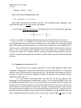
If no internal standard is used and amorphous content is taken to be negligible, the program calculates
the weight fraction for each phase refined, on the assumption that the phases being refined account for
100% of the specimen, via the following relation (Hill and Howard, 1987):
S p (ZMV ) p
W p= N
∑S i (ZMV )i
i=1
where p is the value of i for a particular phase among the N phases present, Si is the refined scale factor,
ZM is the weight of the unit cell in atomic weight units (number of formula units, Z, per cell times the atomic
weight, M, of the formula unit), and V is the volume of the unit cell. For this calculation, the program uses
internally tabulated atomic weights and the refined lattice parameters, scale factors, and atom
site-occupancies. Atomic weights not in the incorporated table may be inserted in line 8.1 of the ICF.
Mole fractions, as well as weight fractions, will be reported at the end of each cycle if the user supplies the
number of formula units per unit cell in ICF line 11.2.
b) With internal standard
DBWS can also make use of an internal standard in Quantitative Phase Analysis. The fact that an internal
standard is to be used is signified with a number in the last position (the twelfth) in line 2.1 of the ICF. The
crystallographic data for the internal standard phase are entered as a set of l1-* lines, just as is done for
the other phases present. The sequence number of this internal standard phase among all of those entered
in this section of the ICF is the ISPHASE number to be entered in line 2.1. The wt% which this phase
contributes to the total sample weight is entered in line 11.2 at the last position in the line in F72 format.
For example, if the standard constitutes 28.42% of the weight of the entire sample, the number 28.42 will
be entered there.
CAUTION: As they stand, above, these QPA calculations do not take into account any
microabsorption effects (see, for example, Taylor and Matulis, 1991). They will be important unless the
linear absorption coefficients are the same, or nearly so, for all phases being analyzed. Therefore, the
neglect of microabsorption effects will generally be a much more serious error in the x-ray powder
diffraction case than in the neutron powder diffraction case.
2. Microabsorption
A beginning effort at providing a microabsorption correction has been made in DBWS-9807. It
involves the use of a particle absorption factor for each phase. Necessarily such a correction also involves
the sizes and shapes, and distributions thereof, of the particles. An approximation to the needed value for
20
DBWS-9807a User's Guide
20.8.00
this particle absorption factor, AFQPA in the ICF, can be obtained from table V, page 368, of the
Brindley paper (1945, Philos. Mag. 36, 347-369) or after evaluation of equation (3) in the Taylor &
Matulis paper (1991, J. Appl. Cryst. 24, 14-17), which is:
t a = (1/Va) ∫exp[-(µa - (µ-bar))] x dVa .
where t a is a particle absorption factor for phase a, the integral is taken from 0 to Va, Va is the particle
volume of phase "a", µa is its linear absorption coefficient, x is the path of the radiation in particle "a" when
diffracted by the volume element dVa, and µ-bar is the mean linear absorption coefficient of the solid
matrix of the powder. The user needs to be cautious with the u-bar. According to Brindley (1945. p.
349), this value must be the mean value for the solid material, excluding the spaces between particles.
Table V in the Brindley paper was computed for spherical particles for use as a 'better than none'
approximation. He well recognized, of course, that a naturally occurring material consisting entirely of
spherical particles of identical size would not be often found.
The value of t (herein coded as AFQPA) for each phase is then used to correct the scale factor for
each phase in the specimen for microabsorption. The equation for phase abundance then becomes (Taylor
and Matulis, 1991)
W p=
S p (ZMV)/ τ p
N
∑S
j
(ZMV ) j / τ j
j=1
E. Codewords and constraints
This effective codeword system has been carried over from Rietveld's original code. A `codeword'
is entered for each parameter. Each codeword has two parts, (1) the designation of a matrix position
for the parameter and (2) specification of the fraction of the calculated shift that is to be applied to this
parameter. The codewords have the form
sdddc.cc
where the ddd digits specify the matrix position for the particular parameter. The c.cc digits specify what
fraction (or multiple) of the calculated shift is to be applied to update the parameter and s is the sign (+ or
-) desired for the applied shift. (A positive shift will be applied if no minus sign (-) is present.) Separately
from the codewords, the user may also supply a group `relaxation' factor to be applied to the
21
DBWS-9807a User's Guide
20.8.00
calculated shifts for all parameters in each of four different groups of parameters. See line 5 of the Input
Control File.
As an example, assume that one wishes to refine the x,y,z coordinates of an atom and that y = x/2 is
required by the crystallographic symmetry. If we let the codewords be given as
x: 131.00,
y: 130.50,
and z: 141.00,
then x and y will be assigned to the 13th normal matrix parameter and z to the 14th. Also, 1.00 times the
calculated shift in the 13th parameter will be applied to x and 0.50 times it to y. The full calculated shift
in the 14th parameter will be applied to z. If, on the other hand, one were to set up the codewords as
x: 131.00
y: -131.00
then the sum of x and y would remain constant.
This `constraint by codewords' feature can be useful in connection with site occupancies also. One
may let two different atoms occupy the same crystallographic site and then determine how much of each
is present in that site by refining their site occupancies under the constraint that the total site occupancy
(atomic per cent) is to remain constant, i.e., by assigning the same codeword to both atoms but beginning
one with a negative sign, so that the applied shift in the occupancy for one atom is the negative of that for
the other.
Zero values for the three c's in a codeword result in the parameter not being refined. However, this
is not always an advisable way to `turn off' a parameter: If some codewords are non-zero but their
applied shifts are set to zero, the result can be the physically unrealistic one of correlation-matrix elements
>100%.
If N parameters are to be refined, then no codeword with a ddd value in the range from 1 to N can
be missing. If any are, the program will stop, a "hole in the matrix" error message will be sent to the
screen (in the PC context) along with identification of the missing codeword. The missing codeword(s)
will also be specified at the end of the aborted main output file.
The number of codewords declared (i.e., entered as non-zero in the Input Control File), whether or
not called for to be refined (line 9 of the ICF), must not exceed the declared size for the array MSZ (see
below).
F. Array size selection and executable program size
Although the issue is rapidly being made moot with the recent great increases in PC memory and
speed, redimensioning of certain arrays was often wanted in order to make best use of limited memory
22
DBWS-9807a User's Guide
20.8.00
and time. This requires making changes in the array sizes at all occurrences in the source code and then
recompiling. With today’s powerful PC’s, one may be able to do the bulk of one’s Rietveld refinement
work by just setting the array sizes to arbitrarily large values and leaving them there. However, if that is
not feasible for some reason, the following are the array-size statements one would most often wish to
modify:
IDSZ = number of data points
IRS = maximum number of allowed reflections (Ka1 + Ka2)
NATS = maximum number of atoms in the asymmetric unit allowed
MSZ = maximum number of elements in the normal matrix, i.e., codewords
NOTE: If the number of codewords declared exceeds the declared value of
MSZ, the excess will be quietly ignored.
NOV = maximum number of reflections allowed to contribute to the intensity
yi at a single data point
The task of changing the numbers in these statements at every occurrence in the DBWS source code
has been greatly simplified in ‘modern’ versions of DBWS: One need only specify the numbers a single
time in the file PARAM.INC and then keep that file in the same subdirectory with the source code file, or
in the path, when the compiling is done.
If the refinement stops and an error message to the effect that "IDSZ is less than MSZ*MAXS"
appears, it will be necessary to increase IDSZ or reduce MSZ or MAXS until IDSZ is equal to or greater
than MSZ*MAXS. The reason is that the space in memory set aside for IDSZ is also used, at different
times, by MSZ*MAXS. MAXS is the number of parameters being varied (line 9 in the ICF).
Obviously, as the matrix size and number of parameters being refined increases, one could quickly run
into the `640K barrier' characteristic of MSDOS and PCDOS. Compilers are commonly available that
can overcome that problem and also make use of the full 32-bit architecture in today's PC's. One such is
the compiler is a part of Microsoft's FORTRAN PowerStation. It makes use of a separate memory
manager program, DOSXMSF.EXE, which then must be in the same directory or in the path with the
*.exe program being used.
The executable versions of DBWS-9807a in the distribution package have been so prepared. Even
under Windows 95/98 the DOSXMSF.EXE file is needed because the actual carrying out of the
operations is still (subliminally!) a DOS activity.
23
DBWS-9807a User's Guide
20.8.00
II. Description of input files
A. The input control file (ICF), (`Tape/Unit 5')
1. What it is and how to create and update it
For compatibility with other programs ( e.g. DB2dI which produces 'd and I' files in the
format needed by the ICDD for the PDF), the name you give this file should include the extension .in or
.inp. This also guards against the propensity Windows 95/98 has for opening a file with a program
selected on the basis of that file's extension.
This file, the ICF, contains the control variables along with the structural and other refinable
parameters. If output of a new ICF is selected (flag 5 for NXT in line 3), the current ICF will be
updated at the end of the last cycle.
The following line-by-line description tells the user how to set up the ICF control file for any
given case. Some users have developed menu-driven preparation programs with which to set up the
input control files. A good program of that sort can certainly be a help to the beginner. However, once
one becomes familiar with the format detail, then to set up a new ICF using an old one as a template, or
to make adjustments to the ICF between runs it is probably quicker and easier to do so by editing the ICF
directly on-screen using a full screen editor. Particularly for making adjustments to the ICF between runs
(of successive batches of cycles), using the the full-screen approach is quicker and easier than plodding
through a menu-driven approach which forces one through preset sequences.
Users who are not fully familiar with the format detail of the ICF, and either do not have or do
not wish to use a menu-driven file-preparation program, will find useful the example ICF placed at the end
of this line-by-line description. It is based on the quartz-plus-alumina case.
An ICF format conversion subroutine is provided for the convenience of users who have on hand the
ICF’s from problems for which they used DBWS-9411. This routine will convert an ICF in DBWS-9411
format into one in the format needed for DBWS-9807. It is called up by entering a negative integer for
NPROF in line 2.1 of the ICF. One then goes through the steps of starting a refinement cycle. As is stated
elsewhere in this Guide, the basic command line to run a Rietveld refinement with DBWS is
PGM DATA ICF OUT
where the actual names are to be entered for the four files indicated. PGM is to be the name for the
executable version of DBWS being used. DATA is to be replaced by the name of either a real data file
(as it is in an actual Rietveld refinement run) or a dummy name, ICF is to be replaced by the name of the
ICF being converted, and OUT is to be replaced by the name wanted for the converted ICF. In special
cases, another file may need to be specified in the command line, that relating a separately determined
whole-pattern background if it is called for in the ICF being converted. See §C1 of Part 2 of this Guide
24
DBWS-9807a User's Guide
20.8.00
for further comment on these files.
2. Line by line instructions for setting up the Input Control File (ICF)
The line-by-line instructions follow. A star (*) before a line number indicates that the line's existence
depends on the value of a control variable.
Line Format Description
1. (A70) TITLE - any 70 characters to be used to label the main output file and the plots
2 Selection of modules in the Refinement model
2.1 (12I4)
JOBTYP
0
X-ray case
1
Neutron case (nuclear scattering only)
2
pattern calculation only, X-ray
3
pattern calculation only, Neutron
NPROF Profile selection
0
Gaussian
1
Lorentzian (Cauchy)
2
Mod 1 Lorentzian
3
Mod 2 Lorentzian
4
Split Pearson VII (asymmetric)
5
pseudo-Voigt (pV)
6
Pearson VII (symmetric)
7
Modified Thompson-Cox-Hastings ('TCHZ') pV
<0 If you set NPROF < 0, an ICF from DBWS 9411 will be converted to DBWS-9807
format and given the name you specified for the output file. See §IIA1 (p. 24) for further
"how to" information.
NPHASE = number of phases ( up to 15 possible )
NBCKGD = background model control
0
- background to be refined (5th order polynomial in 2θ)
1
- background to be read from file tape 3
2,3,.,N - background to be determined by linear interpolation between the N given points
(see instructions for ICF line 6.)
-1 - Alternative, physically based background (Riello, Fagherazzi, Clemente, & Canton,
25
DBWS-9807a User's Guide
20.8.00
1995)
NEXCRG = number of excluded regions
NSCAT = number of atomic scattering factor sets to be added manually
INSTRM = Laboratory _-2θ X-ray, synchrotron X-ray, or neutron diffractometers using a fixed
wavelength radiation
0 - Laboratory ___2θ X-ray data or single detector neutron data
1 - varying incident intensity data (e.g., synchrotron X-ray ) and a single detector or
multiple counters and “fixed” (e.g., constant monitor counts per step) incident intensity
(e.g., neutron CW data)
IPREF= preferred orientation function
0 - Rietveld-Toraya function
1 - March-Dollase function
IASYM = 0 for usual Rietveld asymmetry model
= 1 for Riello, Canton and Fagherazzi (1995) model
IABSR= Choice of surface roughness model
1 - Combination model
2 - Sparks, et al. model
3 - Suortti model
4 - Pitschke, et al. Model
IDATA = Additional identification of the format of the particular i nput diffraction-data file for
the 7 cases in Category 1 (single detector, constant incident beam intensity and wavelength). See
section II.B. Category 1 for further description of these formats and how DBWS utilizes them.
.
0 - the standard DBWS format
1 - free format (see §IIB category 1b)
2 - GSAS format
3 - Philips UDF format
4 - Scintag text format
5 - Siemens UXD format as converted from a RAW file by XCH program ver.1.4 (DOS)
6 - Rigaku ASCII format
Note: It will sometimes be possible to utilize data in some other formats by reducing the format
to one of the above, particularly the free format case (1).
ISPHASE = Sequence number of the internal-standard phase as it appears in the ICF. If ‘0' is
placed here (item 12 in line 2 of the ICF), no internal standard will be used or sought in the
refinement process. If an internal standard is specified here, its weight % of the total sample will
be entered for ISWT in the last position in line 11.2 of the ICF.
26
DBWS-9807a User's Guide
20.8.00
Line
Format
Description
*2.2 (2I4) This line applies only if NBCKGD = -1, i.e., for the 'alternate' background.
All modules on this line are from Riello, et al. (1995)
IAS= Absorption correction
0 - no correction
1 - an 'absorption' (really transmissivity) model for B-B reflection
geometry:
A = 1 - exp(-2mT/sin θ) where m (coded as TMR) is the linear
absorption coefficient for the sample and T (coded as SW) is the
effective sample thickness
FONDO: 'alternate'-background module choice
0 - Standard background
[with options 1& 2, below, the 'standard' polynomial background can also
be used and the Compton and disorder scattering will be added to it.]
1 - Individual isotropic "temperature factors" ( the IUCr recommends the
term ‘atom displacement' rather than 'temperature' or 'thermal') will be
used in calculation of the Compton and disorder-diffuse scattering
contribution of each phase to the background.
2 – Overall “temperature” factor will be used in the above calculations.
3. 4(5I1,1X)
Output control flags.
A flag is set "off" with 0 and "on" with 1, 2 or 3.
(For further information about what these flags control, see §III.D.2)
Flag No.
(1)
(2)
(3)
Flag setting and output called for
IOT =1, observed & calculated intensities at each step
IPL =1, line printer plot file
IPC =1, |structure factors| & R-Bragg
= 2, as for 1 plus |F| , |F| & R- F with the phases with the phases
reported directly as phase angles,
=3, as for 1 plus |F| , |F| & R- F with the Fobs and Fcalc written in
A + iB form to include the phase information
NOTE that this flag must be set `on' (i.e., non-zero)
(i) to cause the inclusion of the possible Bragg reflection positions in the
PLOTINFO file and
(ii) for the DMPLOT display of the calc’d patterns of the separate crystalline
phases to work.
(4) MAT =1, correlation matrix
(5) NXT=1, input file updated from last-cycle results
(6) LST1=1, initial reflection list with indices, multiplicities, breadths, positions,
2
obs
obs
calc
27
calc
DBWS-9807a User's Guide
20.8.00
LP factors, and mixing parameters.
(7) LST2=1, data list (as corrected, e.g., for background)
(8) LST3=1, merged reflection list
(9) IPL1=1, symmetry operators
(10) IPL2=1, Not used. Reserved for possible alternate plot-file creation
11) IPLST:
=1, Stacked summary of the cycle-by cycle value of each parameter, applied shift, and
R-value
=2, output file as for IPLST=1 plus a separate summary of the last-cycle parameters and their
e.s.d.=s.
The following options, 12 - 18, to output the specified plot files are intended primarily for use in the
NBCKGD = -1 case:
(12)
(13)
(14)
(15)
(16)
(17)
(18)
PLOSS=1, Observed data plot file corrected for absorption scattering
PLCAL=1, Calculated 'data' plot file
PLPOL=1, polynomial background plot file
PLCOM=1, Compton scattering plot file
PLDIS=1, uncorrelated disorder plot file
PLAM=1, Plot file of data in 'amorphous' diffraction data file. (Could be for a
polycrystalline rather than an amorphous material.)
PLOTBIG=1, Observed corrected for absorption, amorphous, amorphous plus
Compton, Comp
NOTE: if PLOTBIG is set to 1, PLOSS, PLCAL, PLPOL, PLCOM, PLDIS, and PLAM, will not be
created. To have these plotfiles created, set PLOTBIG=0
(9F8.0)
Fixed parameter values to be supplied by the operator
WAVELENGTH 1 of the incident radiation
WAVELENGTH 2 of the incident radiation
RATIO = intensity ratio e.g., a 2/a
BKPOS= origin of polynomial for background (in °2θ)
WDT = width (range on either side of peak max) of calc. profile in units of HK
CTHM = monochromator coeff. in polarization term of the LP factor:
(1+CTHM*cos 2?)/(sin ? cos ?)
TMR = linear absorption coefficient (cm ) needed for the transparency
correction.
RLIM = A 2? value that determines the 2? range(s) over which the asymmetry
correction is applied.
If IASYM = 0 (Rietveld model) , only the profiles below RLIM are
corrected.
If IASYM =1 (Riello et al. model), the asymmetry correction is applied
1
2
2
-1
28
DBWS-9807a User's Guide
20.8.00
in the regions
2? min < 2? < 90-RLIM
and
90+RLIM<2? <2? max
(so RLIM must be 0<RLIM<90_)
SW = Measured sample Thickness (cm)
5. (I4,5F4,3F8.0)
Some operational choices:
MCYCLE = number of cycles [can not be 0 or no calc’n will be done]
EPS = run terminates when all calculated shifts (not the
actually applied shifts shown in the output) are < (EPS*e.s.d.)
Relaxation factors for shifts by parameter groups:
RELAX 1 - co-ordinates & isotropic atom displacement ("temperature") factors
and site occupancies
RELAX 2 - anisotropic atom displacement parameters
RELAX 3 - profile width, asymmetry, overall atom displacement ("temperature"),
preferred orientation parameters, lattice parameters and overall scale factor.
RELAX 4 -2θ-zero, specimen displacement, specimen transparency, surface
roughness, amorphous scale factor and monochromator band-pass parameters.
Needed for pattern calculation only:
THMIN - starting angle (_2θ) for the pattern to be calculated
STEP - step size (_2_)
THMAX - ending angle (_2θ)
*6.
(2F8.2) if NBCKGD >2 in ICF line 2, enter NBCKGD lines here specifying the
background intensities measured at those NBCKGD points:
POS = position in degrees 2?
BCK = background counts at this position
*7. (2F8.2)
if NEXCRG in line 2 is > 0, enter NEXCRG lines with
ALOW = low angle bound (°2?)
AHIGH = high angle bound
*8. Here is the place to enter scattering factors and scattering lengths which are not in the
If NSCAT>0, enter here NSCAT sets of lines in the formats shown below for your case:
The x-ray scattering factors and neutron coherent scattering lengths that are incorporated here
are those listed in the 1974 version of Vol. 4 or, in some cases, the 1995 Vol. C of the International
Tables for X- ray Crystallography.
29
incorporated ta
DBWS-9807a User's Guide
20.8.00
NOTE that the anomalous dispersion corrections, ?f ' and ?f '', to the atomic scattering factors are
now given in this program for 10 Ka1 wavelengths (2.748510:Ti, 2.289620:Cr, 1.935970:Fe,
1.788965:Co, 1.540520:Cu, 0.709260:Mo, 0.559360:Ag, 0.215947:Ta, 0.209010:W, and
0.180195:Au in A) instead of only those of Cr, Fe, Cu, Mo and Ag given in previous versions of
DBWS. The coefficients provided before were taken from the International Tables for X-ray
Crystallography Vol. 1 (1974) and the now-added ones come from Vol. C (1995). One reason for
providing these additional data is so that scattering factors for working wavelengths chosen from a
continuum (e.g., synchrotron X-radiation) might be better approximated.
a) Line 8 for the X-ray case:
*8-1 (A4,3F8.0) NAM =symbol identifying this set
DFP =f ' (real part of the anomalous dispersion)
DFPP =f " (imaginary part of the anomalous dispersion)
AW - atomic weight (must be included as part of the set)
*8-2 (9F8.0)
Either one line of the form
A1 B1 A2 B2 A3 B3 A4 B4 C,
the coefficients for the approximation to f, as used in the Int'l Tables,
or a set of lines of the form
Posi Scat
where
Posi = (sin _ )/λ__and Scat=f
The set is terminated by a line with -100 in the first position.
If the first form is desired, A2 can not = 0
b) Line 8 for the neutron case:
*8.1 (A4,2F8.0)
NAM symbol identifying this set
DFP - b (scattering length in units of 10-12 cm)
AW - atomic weight (must be included as part of the set)
9. (I8)
MAXS = number of parameters to be refined in this pass
10. Refinable global parameters
10-1. (7F8.0)
ZER DISP TRANS P
-
offset of the 2_-zero point (in _2___
sample displacement
parameter for effect of sample transparency on apparent 2_
surface roughness parameter p
30
DBWS-9807a User's Guide
20.8.00
Q
R
T
10-11 (7F8.0)
*10-2
(3F8.0)
focusing graphite
scattering,
wavelengths,
parameters and
-
surface roughness parameter q
surface roughness parameter r
surface roughness parameter t
FLZER codeword for 2θ-zero point offset
(codeword makeup is described near end of §I of Part 2.)
FLDISP codeword for sample displacement
FLTRNS codeword for transparency coeff.
FLGP codeword for surface roughness parameter p
FLGQ codeword for surface roughness parameter q
FLGR codeword for surface roughness parameter r
FLGT codeword for surface roughness parameter t
[See 2§I.C.5 (this part) of this Guide for explanation of usage and
how to nullify the surface roughness correction.]
AM= scale factor for amorphous, or other, pattern on Tape 11.
MON1 = monochromator band-pass parameter
(if there is a monochromator in the diffracted beam, put MON1=1 and put
MON2=0 if a monochromator works on the incident beam)
______________MON2 = monochromator band-pass parameter ( for a
monochromator, MON1 could be equal to 4 and MON2 could
be equal to 2.
NOTE: MONO1 and MONO2 are needed
mostly when Compton
or other scattering which is not confined to a narrow band of
is important to the experiment. For a description of these
of their values and use, see Riello, Canton & Fagherazzi (1997).
*10-21 (3F8.0)
FLAM= codeword for 'amorphous' (i. e., Tape 11 data) scale factor
FLMON1=codeword for the first monochromator constant, MON1
FLMON2=codeword for MON2
10-3 (6F9.4)
BACK - background coefficients in 'standard' (NBCKGD = 0) polynomial
representation
FBACK - codewords for background coefficients
10-31 (6F9.4)
11. First group of phase-specific parameters: NPHASE (as specified in Line 2) sets of these lines
numbered 11-* are needed, i. e., one set for each phase.
11-1
(A70)
PHSNM = phase name and number
31
DBWS-9807a User's Guide
20.8.00
11-2
(2I4,F8.0,3F4.0, F7.2)
N - number of atoms in the asymmetric unit
FU - number of formula units in the unit cell (used only for
reporting molar phase fraction)
AFQPA - particle absorption factor, t p, for each phase, used in the
microabsorption correction. The value can be taken from
table V, page 368, in the Brindley paper (1945, Philos. Mag.
36, 347-369) or after evaluation of equation (3) in the Taylor
& Matulis paper (1991, J. Appl. Cryst. 24, 14-17). Also see §IID2.
PREF* - preferred orientation direction in reciprocal space, expressed as Miller
indices
ISWT = wt% of the total sample contributed by the internal standard
*Note: In previous versions of DBWS there was a problem with the preferred orientation
correction that could be significant in cases of very high preferred orientation and high symmetry.
That problem has now been corrected.
11-3 (20A1)
SYMB = space group symbol
e.g., P6 /m = P 63/M
P2 2 2 = P 21 21 21
Pb = PB (and sometimes P 1 1 B, etc.)
_
P3 = P -3
Fm3m = F M 3 M
3
1
1
1
(Note the upper case in this symbol. It is needed for some other space groups,
also. The program treats the lower case m in this example as specification of
an hexagonal space group and tries to be accommodating)
For rhombohedral space groups, add H to the symbol to be sure that hexagonal
axes will be used, e.g., R -3 C H, and add R to demand rhombohedral axes.
11-4
11-41
Atom specific parameters: 4 lines for each of the N atoms
(A4,1x,I4,1x,A4,2x,5F8)
LABEL - identification characters for atom
M - multiplicity of the particular site, as given in International Tables for X-ray
Crystallography, Vol 1 or Vol A. It is not refinable.
NTYP - link to scattering data for atom (use all caps): either
(a0 the atom's name from line 8.1, which will access its manually added scattering
factor set or
(b0 its chemical symbol and valence, which will access the incorporated list of
f-coefficients taken from the Int=l Tables. NTYP must start in column 11.
The nominal valence is to be indicated for the X-ray case (e.g. Ca+2) but not
the neutron case.
32
DBWS-9807a User's Guide
20.8.00
x, y, z - fractional atomic coordinates
B - isotropic atom displacement ('temperature') parameter for the atom
So = site occupancy. It should be 1.000 if all equivalent positions are exactly fully
occupied. It is refinable.
11-42 (16X,5F8) CX, CY, CZ =codewords for fractional atomic coordinates
CB = codeword for the atom's isotropic 'thermal' parameter
CSo = codeword for site occupancy
11-43 (6F8)
Beta11, Beta 22, Beta 33, Beta 12, Beta 13, Beta 23
anisotropic 'thermal' parameters
11-44 (6F8)
CB11, CB22, CB33, CB12, CB13, CB23,
codewords for the atom's anisotropic thermal parameters
11-5
11-51 (2F8)
SF = scale factor
BO = overall 'thermal' parameter
11-52 (2F8)
CS = codeword for scale factor
CBO = codeword for overall 'thermal' parameter for the phase
11-6
11-61 (6F8)
U, V, W, CT, Z, X, Y = FWHM ("H") parameters for the expression
HK2=Utan2 θ +Vtan θ +W+CTcot2_ for NPROF = 0-3, 5,6
HK2=Utan2_ +Vtan θ +W for NPROF = 4 (split Pearson VII)
Z, X & Y are used only when NPROF = 7. When not used, their values
must be set to zero (0.00)
11-62 (6F8)
CU, CV, CW, CCT, CZ, CX, CY - codewords for the FWHM parameters
11-7
11-71 (6F8)
A, B, C - cell dimensions a, b, c in Ångstroms
ALPHA, BETA, GAMMA - cell angles a , ß , ? in degrees
11-72 (6F8)
CA, CB, CC, CALPHA, CBETA, CGAMMA - codewords for the cell constants.
Note that within the operations of the program the angles are expressed in terms
of cross
products of the reciprocal-space cell-edge vectors in the program. Thus,
for example,
in a trigonal or an hexagonal system the codeword CGAMMA must be the same as CA
(=CB).
11-8
11-81 (3F8) Enter G1, G2, P, where G1 and G2 are the preferred orientation parameters (see
formulae below) and P is the asymmetry parameter (see RLIM in line 4 for the 2θ range
over
which P is effective)
11-82 (3F8)
CG1, CG2 - codewords for preferred orientation parameters
CP - codeword for asymmetry parameter
If IASYM = 0 in line 2 , the asymmetry function is that given by Rietveld (1969)
33
DBWS-9807a User's Guide
20.8.00
If IASYM = 1, the asymmetry function is that given by Riello et al, (1995).
For both asymmetry models, P and its codeword should be set = 0 when the split
Pearson VII profile function (number 4) is used.
G1, G2 are the preferred orientation parameters used in the formulae (see Part
2,§IC2):
(a) if IPREF = 0 (see line 2.1), Icor = Iobs(G2+(1-G2)*exp[-G1a K2])
(Rietveld-Toraya case, G1 = 0 for no preferred orientation)
NOTE: Expect strong correlation between the Rietveld G1 and the phase
scale factor if strong preferred orientation is present.
(b) if IPREF = 1, Icor = Iobs(G12cos 2? K+(1/G1)sin2? K)-3/2
(March-Dollase case, G1 = 1.000 for no preferred orientation)
where a K is the acute angle between the scattering vector (e.g. dK) and the orientation
direction (e.g. fiber axis direction) specified in line 11-2.
A special feature: With the IPREF = 0 model, setting G1 to any number >99.0 for a phase
causes the program to generate for it only those reflections for which d* is parallel to the preferred
orientation vector PREF specified in line 11.2, as though that phase had a 100% complete fiber-axis
texture.
Note, however, that since the LP factor has not been corrected for the texture, the relative intensities
among orders of a reflection so generated are not correct but are the same as those for a randomly
oriented powder. This is true for all preferred orientation corrections in this program.
Line
Format
Description
11-9
MIXING/SHAPE PARAMETERS
NOTE: for the usual pseudo-Voigt (NPROF=5) the mixing parameter, ? , can vary with
2? as
?__ NA + NB *(2?)
where NA and NB are refinable and NC must be set = 0.
34
DBWS-9807a User's Guide
20.8.00
For the Pearson-VII functions (NPROF=4 and NPROF=6)
the shape parameter, m, is calculated as
m = NA + NB/(2θ) +NC/(2θ)2 (m=m or mL or mH)
where NA, NB and NC are refinable parameters. For NPROF=5, NC
and its codeword must be set =0.
For all other profiles listed (1-3, 7), NA, NB & NC and their codewords must all be set to
zero.
11-91
11-92
11-93
11-94
11-95
11-96
(3F8.4)
(3F8.2)
(3F8.4)
(3F8.2)
(F8.4)
(F8.2)
NA,NB,NC for pV and PVII or the low angle side of SP7
CNA,CNB,CNC ( Codewords for NA, NB, NC)
NA,NB,NC for the high angle side of SP7 (‘Split Pearson VII’)
Codewords for NA, NB, NC on the high angle side of SP7
A, the SP7 asymmetry factor
CA, codeword for A
NOTE: When the Split PVII function is not being used, the parameters and codewords for both m
and A on the high angle side should be set to zero.
When the Split PVII function is being used, one should start with small parameter values and
proceed cautiously, as this function tends to ‘run away’ easily. One strategy that has been used
successfully is that of using the results from refinement with PVII for the initial values in SPVII and
then alternating refinement of the parameters for the High side and the Low side.
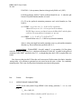
NEXT PAGE: Example of an Input Control File for a simple two-phase case as it appears on
the screen. This is a copy of the QIN file in the QTEST subdirectory on the distribution diskette.
Other examples are provided in the test cases. The ICF for the test case with an internal standard and
an underlying amorphous component may be particularly interesting for advanced users.
35
DBWS-9807a User's Guide
20.8.00
QDATA 2 PHASE TEST CASE QUARTZ+ alumina 8FWHM 13.5.99
0
5
2
0
0
0
0
1
0
1
0
0
00211 10000 10000 000
1.54050 1.54430 .50000 90.0000 8.0000
.8009 1.0000
2 .10 .95 .95 .95 .95
24
.0000 -.0183
.0000
.0000
.0000 1.0000
.0000
.0000 21.0000
.0000
.0000
.0000
.0000
.0000
38.62
116.96
134.91
.00
.00
.00
31.0000 41.0000 181.0000
.0000
.0000
.0000
Alpha quartz
2
3 1.0000 .00 .001.00
.00
P 32 2 1
SI1
3 SI+4
.47002 .47002 .00000 .54982 1.00000
91.00
91.00
.00 190.50
.00
.00490 .00270 .00490 .00140 -.00010 -.00002
.00
.00
.00
.00
.00
.00
O1
6 O-1
.14855 .41914 .11983 1.14715 1.03409
101.00 111.00 121.00 200.50 210.40
.01430 .00000 .01900 .00850 -.00320 -.00420
.00
.00
.00
.00
.00
.00
.658E-02
.0000
11.00
.00
.01959 -.00327 .00594 .00000 .00000 .00000 .00000
160.25
.00
80.25
.00
.00
.00
.00
4.9139 4.9139 5.4052 90.0000 90.0000120.0000
61.00
61.00
71.00
.00
.00
61.00
1.00000 .00000 .16680
.00
.00 130.50
.5100
.0000
.0000
140.50
.00
.00
.0000
.0000
.0000
.00
.00
.00
.0000
.00
PHASE 2
ALPHA ALUMINA
2
6 1.00001.001.00 .00
.00
R -3 C H
AL1
12 AL+3
.00000 .00000 .34998 .80000 1.00000
.00
.00 220.50
.00
.00
.00000 .00000 .00000 .00000 .00000 .00000
.00
.00
.00
.00
.00
.00
O1
18 O-1
.31309 .00000 .25000 1.00000 1.00000
230.10
.00
.00
.00
.00
.00000 .00000 .00000 .00000 .00000 .00000
.00
.00
.00
.00
.00
.00
.469E-04 3.2945
51.00 240.50
-.03121 -.00327 .02430 .00000 .00000 .00000 .00000
170.10
.00 150.30
.00
.00
.00
.00
4.7609 4.7609 12.9962 90.0000 90.0000120.0000
.00
.00
.00
.00
.00
.00
1.00000 .00000 .00000
.00
.00
.00
36
2/24
LINE 2.1
LINE 3
35.0000
.0000
CYCLS EPS RELAX P_CALC
PARAMS REFINED
ZER DISP TRANS p q r t
CODEWORDS
BACKGROUND
CODEWORDS
PHASE NUMBER 1
#ATMS #FU AFQPA PREFDIR ISWT
SPACE GROUP
LBL M NTYP x y z B So
CODEWORDS
BETAS
CODEWORDS
LBL M NTYP x y z B So
CODEWORDS
BETAS
CODEWORDS
SCALE Bo(OVERALL)
U V W CT Z X Y
CELL PARAMETERS
PREF1 PREF2 R/RCF_ASYM
NA NB NC (MIX_PARAMS)
NA NB NC (HIGH SIDE)
PEARSON ASYM.FACTOR
PHASE NUMBER 2
#ATMS #FU AFQPA PREFDIR ISWT
SPACE GROUP
LBL M NTYP x y z B So
CODEWORDS
BETAS
CODEWORDS
LBL M NTYP x y z B So
CODEWORDS
BETAS
CODEWORDS
SCALE Bo(OVERALL)
U V W CT Z X Y
CELL PARAMETERS
PREF1 PREF2 R/RCF_ASYM
DBWS-9807a User's Guide
20.8.00
.5850
.00
.0000
.00
.0000
.00
.0000
.00
.0000
.00
.0000
.00
.0000
.00
NA NB NC (MIX_PARAMS)
NA NB NC (HIGH SIDE)
PEARSON ASYM.FACTOR
II.B The observed data file, Tape/Unit 4
Tape 4 contains the observed (experimental) data from the 'diffractometer'. The format can be in any of
several formats, depending on the type of instrument and the software used on it. The acceptable formats
are here divided into categories which differ according to whether the incident beam intensity is fixed or
varying and whether a single or multiple detectors are used. All require 'steps' consisting of equal
increments in 2?.
The data format type is specified in the ICF by a combination of flags in line 2. For case (a) of Category
1 and for categories 2 and 3, set the flag IDATA=0. (That is the flag in position 11 in line 2.) For other
cases in Category 1, the IDATA flag will be set to other values, as is shown below. For case (a) of
category 1 and for categories 2 and 3 (IDATA=0), the data format is further identified in ICF line 2 by
the combination of the settings of flags 1 (JOBTYP) and 7 (INSTRUM).
Category 1:
Constant incident x-ray or neutron flux and a single detector collecting x-ray or neutron data at
equal increments in 2θ (JOBTYP = 0 or 1, INSTRUM = 0 )
Case (0): The 'standard' DBWS observed data file (Tape/Unit 4) . IDATA= 0
The first line contains the variables START, STEP, STOP, and DATAID in (3F8.3, A48) format:
START- beginning angle in degrees 2θ
STEP- step size in degrees 2θ
STOP- last angle in degrees 2θ
DATAID- An alphanumeric string identifying the data.
The rest of the file consists of the intensity data themselves in (8(F7.0,1X)) format. There may be,
but need not be, a ninth column listing the 2? angle for the last datum in each row.
NOTE: The START angle assigned here must correspond to that of the first datum not in an
excluded region. The STOP angle can be any angle less than that of the last datum in the file. One
can select any desired a ngular range for the refinement, without removing any data from the file,
by
(i) declaring an excluded region (NEXCRG in line 2 of the ICF) and specifying its bounds (line 7 of
the ICF) as beginning at the START angle declared in the first line of the data file and ending at the
desired beginning angle for the calculations and
(ii) assigning the desired ending angle to STOP.
37
DBWS-9807a User's Guide
20.8.00
Case (1): Free format. IDATA= 1
The first line contains the variables START, STEP, STOP, and DATAID in (3F8.2, A48) format, just as
in case (0). The rest of the file consists of the intensity data, only, in free format. Any number of columns
of any width are allowed. The delimiters are commas or spaces. Angle data are not allowed.
Case (2): GSAS 'standard' format. IDATA= 2.
The DBWS program searches through the header material that starts with 'BANK' to find the start angle,
step size, and stop angle. The rest of the file consists of the intensity data in format 10(I2,F6.0). No
commas or angle data are allowed. Note that in the 'standard' GSAS format for the data all rows must be
filled out to 80 characters. Use spaces if necessary to fill out the row(s).
Case (3): Philips UDF format. IDATA= 3.
The program searches through the (voluminous!) header material for the lines "DataAngleRange" and
"ScanStepSize", from which it gets the start angle, stop angle, and step size information. It then looks for
the start of the data file immediately following the "RawScan" line. The intensity data are expected to be in
format (8F8,1X) where X in this case is actually a comma
Case (4) Scintag "text" format. IDATA= 4.
The program searches through the multi-line header for the start angle, step size, and stop angle. It then
ignores the 'axis' blocks and goes to the four column main output: angle, count, time, and e.s.d..
The DBWS program then reads the intensity data from column 2 and ignores the other three columns
Case (5) Siemens UXD format. IDATA = 5.
As in cases 2-4, above, the program searches through the header material to find the start angle, step size
and stop angle (or step), ignores the rest of the heading material and proceeds to read just the intensity data
(in counts) from the rest of the file.
38
DBWS-9807a User's Guide
20.8.00
Case (6) Rigaku ASCII format. IDATA = 6.
.
The program proceeds as in (5).
Category 2.
Varying incident x-ray flux (e.g., synchrotron x-radiation) and a single detector collecting data in
equal increments of 2?.
(JOBTYP = 0, INSTRM = 1, IDATA= 0).
DBWS programs use the normalized intensity data both directly as the observed data and, with the other
data provided in the file, to reconstruct the originally observed total count at each step and, from that, to
assign the statistically correct weight to each observed step intensity yio .
The first line contains the variables DATE (for date or place) and DATAID in (A5,A56) format:
Line Format
Content
1 (A5,A56) DATE - Identifies the format of the data. Currently supported values are (a) OCT85,
respectively.
FEB86,
DATAID - an alphanumeric string identifying the data.
2
(I8,F8,G10) NRANGE - No.of blocks in which the data are written.
CHMBRI - Value of incident-beam counts-per-step to which all data are to be
normalized. (DBWS assigns the weights on the basis of the actually observed,
not
normalized, number of counts at a step.)
TAUK - Coefficient for deadtime correction for the diffracted-beam detector (in
seconds)
3. For each of the NRANGE no. of blocks:
3.1 (6F8) ANGMIN - beginning angle for this block in °2?.
STEP - step size in °2? (identical for all blocks)
ANGMAX - last angle for this block in °2?.
STPTIM - counting time at each step in seconds
OFSTI0 - "dark current" counts-per-step in the incident-beam monitor
OFSTI1 - "dark current" counts-per-step in the diffracted-beam detector
3.2
IPTS lines of data in one of the following formats, where IPTS is the no. of data points
(24X,F7,1X,F7) for DATE = (OCT85 OR FEB86)
39
(i.e., 2?
DBWS-9807a User's Guide
20.8.00
(51X,F10,1X,F10) for DATE = AUG86
(37X,F9.0,1X,F9.0) for DATE = SRS83
(29X,F9.0,10X,F9.0) for DATE = SRS91
where Io and I1 are the data entered in F format and
I0 - actual total counts from the incident beam monitor at this step
I1 - actual total counts from diffracted beam detector at a given step
Also, I1 comes before I o in the OCT85 and FEB86 formats and vice versa in the other three.
Category 3. Fixed wavelength, constant intensity (or monitor count) neutron beam (for example)
incident and multiple diffracted-beam detectors , but not all detectors contribute to the count at every
step (e.g., instruments D1A and D2B at ILL and the HRNPD at BNL).
(JOBTYP = 1, INSTRM = 1, IDATA= 0)
The first line contains the variables START, STEP, STOP and DATAID in (3F8,A56) format.
START - beginning angle in °2?.
STEP - step size in °2?.
STOP - last angle in °2?.
DATAID- An alphanumeric string identifying the data.
The rest of the file consists of the data and the no. of counters in (10(F2,F6)) format:
NCOUNT - no. of counters
Y(I) - Average intensity
DBWS programs use these data to reconstruct the originally observed total count at each step and, from
that, to assign the statistically correct weight to each observed step intensity yio .
II.C. Background data file 1) `Tape/Unit 3'
If NBCKGD = 1 (ICF line 2), this file contains background data to be subtracted from the
diffraction pattern data (Tape 4). The start angle, step size, stop angle, and data format must be the same
as they are in Tape 4. In the present version of the program, this requirement probably means that this
option for Tape 3 can only be used when the experimental pattern data are in the ‘standard’ DBWS
format, (8(F7.0,1X)).
If NBCKGD <1, Tape 3 is used only as a scratch file.
40
DBWS-9807a User's Guide
20.8.00
If NBCKGD ≥2, (a) Tape 3 is used only as a scratch file and (b) the background will be interpolated
from the NBCKGD number of intensity/angle points listed in the ICF by the operator according to the
instructions in ICF line 6.
2) Tape/Unit 11
If NBCKGD = -1, this file contains “background” data for which the scale factor can be
refined in the Rietveld refinement process. These data may be partly calculated (e.g., Compton and
disorder-diffuse scattering) or real data from an amorphous or other sample, or both. (See Reillo,
Fagherazzi, et al., 1995)
For the Tape 11 data (i.e., for the amorphous or other material for which only the scale factor is to
be refined):
The first line contains the variables START1, STEP1, STOP1, TMV, SW1, DATAID1 (6F8.2,
A16):
START1- beginning angle in degrees 2_, it must be equal to START in the main
data file (tape 4)
STEP1- step size in degrees in 2θ, it must be equal to STEP in the main data file
STOP1- last angle in degrees 2θ, it must be equal to STOP in the main data file
TMV-linear absorption coefficient for the amorphous phase (cm )
SW1- sample thickness (cm)
DATAID1- an alphanumeric string identifying the data
-1
The rest of the file consists of the intensity data in free format.
These background data from Tape 11 are called for by inclusion of the file name in the fifth position
on the command line used to start a refinement. For example:
PGM DATA ICF OUT TAPE11
41
DBWS-9807a User's Guide
20.8.00
III. Description of Output files
A. Plot files.
1) PLOTINFO
A file called PLOTINFO (identified internally as Unit 9) is generated by DBWS. It is an alpha-numeric
file containing the title information from line 1 of the Input Control File, a separately labeled listing of the
geometrically possible Bragg reflection positions and their Miller indices h,k,l for each phase involved in
the refinement (flag 3 in line 3 of the input control file must be `on' for these positions to be included), and
a listing of the calculated and observed intensities at each step, i.e., yic and yio. With PLOTINFO, the
DMPLOT program (offered as a Shareware item with the PC version of the DBWS program) can
produce a plot of the calculated and observed patterns, the difference plot, and position markers for the
possible Bragg reflections from each of the phases involved either (a) on-screen, which can then be
dumped to a printer to provide a hard copy, or (b) directly via a plotter. With PLOTINFO and the
additionally generated binary file, PLOTINFO.BIN, DMPLOT can display on screen (1) the Miller
indices for the various reflections and (2) the component patterns (one for each phase) which make up the
total calculated pattern in a multiphase refinement. DMPLOT also offers Mouse control, dynamic `zoom',
on screen display of 2? and d values at the cursor position, and several other advanced features. Apart
from Rietveld refinement plots, DMPLOT can also display up to 4 `raw data' patterns simultaneously on
screen and move them around relative to each other. To use DMPLOT in this mode, the raw data file
names must have the extensions *.rit for x-ray data *.neu for neutron data.
It should be a relatively simple matter to make a useful Rietveld refinement plot from PLOTINFO
with any of several other generally available software packages.
2) PLOT FILES that can be generated when NBCKGD = -1 (Riello, et al. case) and one
or more of flags 12-18 in ICF line 3 is/are set to 1.
File name
Flag no.
PLOTOSS
12
Total observed plot file corrected for ‘absorption’ scattering expressed in
counts
PLOTCAL
13
Total calculated plot file, obtained by summing the background
PLOTPOL
PLOTCOM
14
15
Background representation obtained from refining it with a polynomial
Plot file for total Compton scattering contribution to the background,
corrected for the monochromator band-pass function if a
is present on the diffracted beam
monochromator
PLOTDIS
16
Description
Total uncorrelated, calculated disorder contribution to the
42
DBWS-9807a User's Guide
20.8.00
background
PLOTAM
17
Plot of Tape 11 data (e.g., "amorphous") corrected for ‘transmissivity’
PLOTBIG
18
Multiple columns file, to do plots using commercial programs like
TM
Origin _ ExcelTM etc.. It contains, in each column respectively,
PLOTOSS, PLOTCAL, PLOTAM, PLOTAM + PLOTPOL, PLOTAM
+PLOTPOL +PLOTCOM, PLOTAM + PLOTPOL + PLOTCOM +
PLOTDIS, and weighted residuals defined as Σ(Ycal -Yobs) 2⁄Σ(Yobs)]
NOTE: if the PLOTBIG flag in ICF line 3 is set to 1, the other 6 PLOT*
files will not be created. To have those plotfiles created, set PLOTBIG=0
B. An updated Input Control File (`Tape 5'), which is updated with the final-cycle parameters, is
output if flag 5 in line 3 of the ICF is set at 1. Routinely, one does want this file to be generated so that the
next step of the refinement process can proceed from the last ending point without extra keyboarding.
NOTE:. The updated ICF is written over the old one, which is then lost.
C. Output to terminal during run
This file is assigned to the terminal when the program is run interactively, e.g., when the program is
run on a PC or workstation. It displays the program name (DBWS) and version, the sizes declared for the
five most frequently redimensioned arrays, the title information for the run, the number of cycles called for,
the number of parameters being refined, the START and STOP angles plus the step size, and a dynamic
series of dots marking the progress of the program through the current cycle. At the end of each cycle, it
reports R-p, R-wp, R-exp, and S (GofF). We thank Dr. H. Marciniak for his very useful additions of
much of the information content and the dynamic display to this output-to-terminal. A compilation of R-p
and R-wp cycle-by-cycle values are saved to the working directory as “Unit 7".
D. The main output file - (`Tape 6').
1. Standard parts of the main output file.
All control variables and structure parameters are printed out so that a given run can be
reconstructed unambiguously. At the end of each cycle, the parameters with their shifts (applied, not the
full calculated ones), the quantitative phase analysis result (wt. % and molar %), plus various numerical
43
DBWS-9807a User's Guide
20.8.00
criteria of fit (e.g., R's and e.s.d.'s) and related values are printed out. See §III.E for definitions of the
various criteria and comments about their interpretation.
2. Optional outputs.
The following optional outputs, mostly in the main output file, are selected (1, 2 or 3) or suppressed
(0) by the settings of the flags in line 3 of the ICF (input control file). They are numbered below in the order
of their appearance in ICF line 3.
Flag #
Items output if flag setting is 1 or, for flags 3 and 11, 1 or 2.
1. Observed and calculated intensities. After the last cycle, a table of the observed and calculated
counts at each step can be printed.
2. Line-printer plot. (For use when there is nothing else available!)
3. It is this same flag which must be set `on' to cause the inclusion of the possible Bragg
reflection
positions in the PLOTINFO file. Different choices of the flag ("IPC") value produce these
results in the main output file:
IPC =1, |structure factors| & R-Bragg
=3, as for 1 plus |F| , |F| & R- F with the Fobs and Fcalc written in A + iB form
to include the phase information
= 2, as for 3 except that the phases are reported in terms of the phase angles
2
obs
calc
4. Correlation matrix.
5. This flag controls creation of the updated input control file, discussed in §III.B, above,
which is output s
6. Reflection list - A list of the reflections generated from each phase with the initial input
profile-component mixing parameters.
7. Corrected data list - A list of the point-by-point intensity data as corrected for
background, the assigned weight, and the identifying number of the highest angle and the
lowest angle reflections which contribute to the data point. The reflection list is sorted so that
contributing reflections may be indicated by giving a pair of integers. K1 is the number of the
reflection in the merged list at the smallest 2? angle contributing to the point. K2 is the highest
angle (2?) reflection for contribution.
8. Merged reflection list (includes hkl, FWHM, 2?, Ic, Io, & R-Bragg.)
9. Listing of the symmetry operators used
44
paramete
DBWS-9807a User's Guide
20.8.00
10. Plot files which are stored and printed out separately. See part A of this section, §III.
11. A stacked summary of the cycle-by-cycle values of each parameter, another of the R
generation.
E. Definitions and interpretations of the numerical criteria of fit.
1. Numerical criteria
a) The standard deviation, a mathematical statistic that should not be confused with
e.s.d. = s jj = { M-1jj S (yoi-yic)²/(N-P+C) }1/2
where
M-1jj is the corresponding diagonal element in the inverted normal matrix,
N is the number of observations,
P is the no. of parameters that are refined, and
C is the total number of constraints.
b) The numbers after "R-factors" are:
R-p = 100 S|yoi-yci|/S|yoi|, the pattern R-factor.
R-wp = 100 { S wi(yoi-yci)²/S wi (yoi)² }1/2, the weighted pattern R-factor.
R-expected = 100 { (N-P+C)/S wi (yoi)2}1/2,
where N is the total number of data points ("observations"), P is the number of parameters
adjusted, and C is the number of constraints applied.
S is the "goodness of fit", the ratio R-wp/R-expected.
Calling for the reflection list (flag 3 in line 3 of the Input Control File) causes R-Bragg and R-F
to be printed out at the end of the final cycle, where
45
values, a
DBWS-9807a User's Guide
20.8.00
R-Bragg = 100 S|"Io "- Ic|/S"Io",
which is the R-value for Bragg intensities, and
R-F = 100 S| |F"obs"| - |Fcalc||/ S |F"obs"|,
which is the R-value based on the deduced "observed" and calculated structure amplitudes. Some
workers find this useful in ab initio structure determination.
c) D-W D is the Durbin-Watson statistic, d, (Hill and Flack, 1987). It is included in the output from
N
d = ∑ ( ∆ y i - ∆ y i-1 ) /
2
i= 2
NDELTA
∑
yi
2
i =1
each cycle as a possibly useful additional indicator of the progress of the refinement. It is given by
where ?yi = wi(yio - yic). In DBWS-9411 and 9807 the wi's are all taken to be 1.00 in order to yield
the unweighted form. That is preferred by some statisticians over the weighted form discussed by Hill and
Flack (1987) and given in Schwarzenbach, et al. (1989). (The weighted form is used in DBWS-9006.)
This d is sensitive to misfit of the calculated and observed reflection profiles, both because their areas may
differ as well as their positions and, importantly, because their shapes may be inherently different.
Consider, for example, how d would be small for a symmetric calculated Lorentzian profile used to fit a
symmetric Gaussian experimental profile even if the two profiles had the same peak positions, peak heights
and areas.
2. A Comment about interpretation of R's:
R-p and R-wp are not directly comparable to the R-values obtained in single crystal
refinements. R-Bragg and R-F come closer to that mark but suffer from the fact that "Io" is not directly
observable where reflection profiles overlap (the usual case). The actual observed intensity in a clutch of
reflections is parceled out among the component reflections in proportion to the calculated reflection
intensities to produce the "Io's".
As is well known to experienced users, R-p and R-wp are also very sensitive to the
background level if the background is included in the yoi's above. It is so included by DBWS-9807 when
the refinable background model is used. It is obvious that R-wp (for example) will be decreased as the
background level is increased (signal-to-noise level decreased) because it is easier to get a good fit to a
function that varies slowly and near to monotonically with angle, as the background does, than to one that
has many sharp maxima along the way, as the pattern of the Bragg reflections does. Experienced users
therefore do not expect to judge the relative quality of Rietveld refinement's made with different data sets
and even different materials by the relative R-wp or R-p values. Those R-values are, however, good
46
DBWS-9807a User's Guide
20.8.00
indicators of the progress of a particular refinement. Obviously, it would be helpful in some cases if the
DBWS programs output the various R-values as calculated both with and without the background
included. Coding for that would probably not be very difficult, but it has not yet been done. Users,
particularly those to whom this effect of background is a new thought, may find interesting the Jansen,
Schäfer and Will (1994) paper in which are given specific examples of the effects of excluding vs including
the background in R-value calculations.
Almost all users may find interesting the Cox and Papoular (1996) paper on R-factors, Errors and
Significance tests. Although ‘Synchrotron Data’ is a part of the title, the content of the paper has much
wider potential applicability.
47
DBWS-9807a User's Guide
20.8.00
PART 3. Further comments on using DBWS-9411 AND 9807 with a PC
A. Compiling
The executables provided in this distribution package and used for the test-case examples
given here were produced with the Microsoft FORTRAN PowerStation compiler. It has the capability
of producing executable versions which can make use of nearly all of the RAM available (i.e, not limited
to 640K). We have run some of the executable versions under MSDOS 6.0. We suppose, but have
not demonstrated, that they would also run under some older versions of MSDOS. They also ran very
well in the Windows 95/98 environment. See §C2 of Part 3.
B. Plots
1. Production and character
Although it has no plotting code embedded in it, DBWS-9807 does produce the output file
PLOTINFO which can be used by other programs to make `Rietveld refinement' (RR) plots.
The separate plotting program, offered as SHAREWARE, for which the MSDOS
executable code is here included, is DMPLOT.EXE. It will use PLOTINFO or specified other file with
the same structure to make a plot with selectable X and Y magnifications, either on-screen or (for
better resolution) with many HP and similar plotters, of the observed and calculated patterns, the
difference, and the Bragg-reflection position markers for all phases. The on-screen plots can then be
dumped to a laser or dot-matrix printer. The program works with various commonly available graphics
adapters for both monochrome and color monitors of various resolution capabilities. DMPLOT has
many very useful features, including separate plots for the phases, multiple zoom, d and I readouts, etc..
See the “Read.me” file in the DMPLOT subdirectory on the distribution diskettes.
DMPLOT is the property of its author, Dr. H. Marciniak. The executable version is offered here
as a 'Shareware' item, which means that you, the user, should try out the program and, IF you find it really
useful, you should send the requested fee to the author. Dr. Marciniak's address is included on one
of the screens you will see when you use his program.
The usual format of the RR plots is that the observed pattern is plotted in the upper field as
a series of unconnected symbols (dots, squares, or e.s.d. bars) the calculated pattern is plotted in the same
field as a solid line formed by straight line connections of adjacent points, the difference pattern (observed
minus calculated) is plotted in the lower field as a continuous curve, and the positions of the geometrically
possible Bragg reflections are indicated as a series of short vertical lines in the intermediate field. To let
them be distinguished, the `Bragg markers' for each phase are plotted at different levels in the intermediate
field to let them be distinguished. However, the user may choose other positioning of the plots and other
48
DBWS-9807a User's Guide
20.8.00
symbols or connections.
The RR plots in the FIGURES section are screen dumps of plots produced with DMPLOT.
The jagged appearance of the enlarged plot sections is due to the pixel size, not to any problem with
DMPLOT. Had we used the output-to-plotter feature of DMPLOT, this jagged appearance would not
be present.
2. Adroit use - an example
In the following figures one may see an example of the use of RR plots to guide fine tuning
of a refinement from a `maybe we can quit here' stage to a very much better stage. The data used are in
the QTEST subdirectory in the distribution package. The codeword numbers assigned to the various
paraemters varied are shown following table.
Codeword numbers for parameters in sample used for Figures 1-5.
I = quartz phase
II = alumina phase
Codeword
Parameter(s)
Phase
1
2
3
4
5
6
7
8
9
10
11
12
13
14
15
16
17
18
19
20
Scale factor
displacement of sample all
background coeff. #1
background coeff. #2
Scale factor
a, b
c
W - (in FWHM)
x,y of Si
x of O
y of O
z of O
asymmetry (profile)
NA - mixing parameter
W
U
U
background coeff. #3
B for Si
B for O
I
all
all
II
I
I
I
I
I
I
I
I
I
II
I
II
all
I
I
49
DBWS-9807a User's Guide
20.8.00
21
22
23
24
So (occupancy) for O
z of Al
x of O
B(overall)
I
II
II
II
Figures 1 - 5 show the progressive improvement in the refinement, done with a part of the QDATA
(20.12 - 60.10 °2?), as the `zoom' feature first revealed the character of the remaining misfit at each stage
and then appropriate changes were made in the calculated profile tail lengths and in the number and
selection of parameters varied. In the process, the Goodness-of-Fit parameter went from being >2.0
(usually not considered to be very good) to 1.40 (usually considered to be quite good) and R-wp went
from 18.1% to 13.77%. From the data in the heading for each plot and the preceding table of the
codewords numbers of the parameters varied in this refinement sequence, one can deduce just what was
changed at each step. The length set for the calculated profile tails is the number of FWHM's given in the
heading. The note resembling a fraction that appears there, i.e., 5/21, is the (number of cycles in this
pass)/(number of parameters varied). From the following table, one can see which parameters have
codeword numbers small enough so that they were included in the number of parameters varied, 21 in this
case.
Figure 6 is the RR plot corresponding to data in the subdirectory FTEST on the distribution
diskette. Fig. 6a shows the plot for the range of the fluorapatite data used (15 - 90 °2?). Figure 6b shows
a closeup of the most troubled looking portion of Figure 6a. On such inspection, and noting that the R-exp
is unusually small, one sees that the refinement appears to be better than would be expected from the GofF
('S', the "Goodness of Fit" ) alone.
Figure 7 is an enlarged portion of a RR plot from a recent PZT study of Dr. Paiva's. It is an
example of how DMPLOT can display the separate calculated patterns in a multiphase refinement. In this
case, there are four phases.
C. Execution procedure with a `PC'
1. In DOS
A possible Start-up routine:
Create a subdirectory on the hard disk
Copy all related files in to that subdirectory, including the executable versions of the
programs you w
Make sure that you are using a version of your ICF that is compatible with this version of the DBWS
program. You can use DBWS-9807 to convert an ICF used for DBWS-9411 to a format compatible
with DBWS-9807. See the instructions given in Part 2, §IIA1.
50
DBWS-9807a User's Guide
20.8.00
Execution:
Modify the INPUT CONTROL FILE (ICF) and DATA files as needed, using the instructions in
Part 2 of this guide for the Input Control File (`Tape 5') and the observed data file (`Tape 4').
To run the program in the MSDOS environment, on the command line type:
DBWS DATA INPUT OUTPUT [Tape 11] [Tape 3]
using single spaces between the entries, the actual file names you have for the executable program, the
observed data file, the Input Control File, and your choice of output file name, respectively. Tape 11 and
Tape 3 relate to (a) data representing an ‘amorphous’ component and (b) a predetermined or assumed
whole-pattern background, respectively. For most work, they are not used.
2.Using DBWS in a Windows environment
Although they are DOS programs, the executables provided for DBWS can run in the Windows 95
(also 98 and NT) environment in a DOS window automatically called up when the program execution
starts. Advantage can thereby be taken of some of the 'drag and drop' and file handling conveniences of
Windows 95/98.
In a Windows environment you may either (1) work in a DOS window into which you can
drag-and-drop the command line files, in sequence, or (2) you can drag-and-drop them onto the
command line that is brought up when you select "run" from the Windows Start Up menu. The second
option here takes more advantage of Windows features and eliminates retyping of the same command
line..
With a good text editor that will operate in Windows and not leave ‘tracks’ (e.g., control characters
and anything else not compatible with ASCII text), one may enjoy essentially all of the benefits of the
Windows operating system while using DBWS.
The text editor that we are presently using with considerable satisfaction is the Programmer’s File
Editor (‘PFE32') from Alan Phillips at Lancaster University (UK). It is available free from his website:
http://www.lancs.ac.uk/people/cpaap/pfe/
We find it is very helpful to keep a 'Shortcut to Pfe32.exe' icon on our 'desktop', preferably in or near
one corner of the screen where it can be accessed with little or no movement of the windows that are open.
A procedure for using DBWS under Windows that has worked well for us
51
DBWS-9807a User's Guide
20.8.00
The first step in the procedure is to prepare all of the files that will be needed for the next set
of Rietveld refinement cycles (the next 'run') and to put them in one subdirectory not far from the root
directory. The results worth keeping can be transferred later from this 'working directory' to another, more
comprehensive file directory. The purpose of the 'not far' specification is to maximize the probability that
files generated during the refinement run will find their way back to your working directory rather than
going off someplace where you have to hunt for them, e.g. in the Windows directory. *
The files that are always wanted in the working directory are (1) the executable version of DBWS to
be used (e.g., DB9807.exe), (2) the DOS extender file DOSxmfs.exe, (3) the data file for the particular
case (e.g. case1.dat), (4) the input control file (the “ICF”, e.g., case1.in), (5) the output file named as
wanted (e.g., case1.out. It can be an empty file at this point), and (6) the two DMPLOT files (i. e.,
dmplot.exe and dmplot.cfg) which you will use to examine the refinement results as you proceed. Other
files that are needed in this working directory for some refinement options are the 'amorphous' data file
(Tape/Unit 11) for which the scale factor will be refinable and a file containing predetermined
whole-pattern background data (Tape/Unit 3) which are to be subtracted from the experimental
diffraction pattern data.
The next step is to click on START (lower left corner of your screen) and select ‘run’. That opens a
command line (labeled 'open') into which you will drag-and-drop the needed files from the working
directory in the sequence: program file, data file, ICF, and 'out' file. For some refinement options you will
have to put a fifth and sometimes a sixth file name on the command line. These are the file names for the
data in Unit 11 and in Unit 3, described in the previous paragraph. If both are used, the file containing the
whole-pattern 'amorphous' component data is entered in the fifth place. Be sure to put all of the files that
will be needed into the working directory first so you can drag-and-drop them onto the command line.
By doing so you will avoid the tedium and typographical errors of having to type in both the file names and
the paths to them.
If all has gone well, when the specified number of cycles is completed you will find in the
working directory the new 'out' file, the ICF (rewritten if you called for that with flag 5 in line 3 of the ICF),
a PLOTINFO file, a POTINFO.BIN file and a file called 'unit 7' along with the files that have not been
changed. You will probably want first to look at the 'Rietveld' plot resulting from the run just finished.
You can do that by dragging PLOTINFO onto DMPLOT.EXE and following the screen instructions. The
PLOTINFO.BIN file is the one that makes it possible for you
(1) to see all of the reflection indices for all phases by simply pressing the F3 key and
(2) to see the individual calculated patterns for all phases superimposed on the standard Rietveld plot.
You can now look at the content of, and edit, any text file by dragging it to the desktop and dropping
it on the Pfe32.exe icon. If you have enough information from the plot to make wise choices now for
improving the fit, you may wish to go directly to editing the ICF for the next run (i. e., batch of cycles).
52
DBWS-9807a User's Guide
20.8.00
You do that, of course, by dragging the ICF to the Pfe32.exe icon to open the file and then using the Pfe
features to do the desired editing. You may want to look at the 'unit 7' file to see, again, the R values that
appeared on the screen during the run. At some point, you will want to look at the 'out' file, perhaps print
parts of it, (all easily done with Pfe32.exe) and perhaps check the magnitude and pattern of the parameter
shifts, the calculated e.s.d.'s for them, and the correlation matrix in order to guide your choice of changes
to make in the ICF for the next run.
When you have finished setting up the ICF for the next run, you can press the Start button and then
'run', again. The command line you used before now appears. If the file names have not changed you need
do nothing but press the 'OK' button and the computer takes off on the next set of refinement cycles while
you look on with delight at seeing all this work being done for you while you just sit there.
------------------------------------------------------------------------------------------------*If you do not keep all of the needed files, including program files, in the working subdirectory, the
problem may then occur that a file created during the operation of the program will go to another
directory. That will usually be the Windows directory, where at t he expense of some effort and
exasperation it can be captured and brought back to the working directory. However, DBWS-9807
includes some special programming that is supposed to avoid that problem by sending a newly created file
(e.g., PLOTINFO) to the same place that the main output file (e.g., *.out or whatever other name was
specified in position 4 of the command line) goes. To assure that the place to which it goes will be the
working directory, it is necessary either (1) to have the *.out file in the working directory before it is
dragged over and dropped on the DOS window in which the DBWS program is about to run or (2) to
type out, in the command line being constructed in the window, the full path for the *.out file --- which,
of course, gives but little advantage over the plain DOS procedure. With option (1), above, the *.out file
thereby brings its path information with it. This feature has worked well for the PLOTINFO and
PLOTINFO.BIN files in our PC operating system (WIN95/98 with a PII chip).
53
DBWS-9807a User's Guide
20.8.00
REFERENCES
Caglioti G, Paoletti A, and Ricci FP, (1958) Nuclear Instruments and Methods, 35, 223-228.
Cheary, R. W. and Cline, J. P., (1994) Adv. in X-ray Analysis 38, 75-82.
Cox, D. E. and Papoular, R. J., (1996) Mat. Sci. Forum, v. 228-231, pp. 233-238.
Hastings JB, Thomlinson W, and Cox DE (1984) J. Appl. Cryst. 17, 85-95.
Hill RJ and Flack HD, (1987) J. Appl. Cryst. 20, 356-361.
Hill RJ and Howard CJ, (1987) J. Appl. Cryst. 20, 467-474.
Jansen E, Schäfer W, and Will G, (1994) J. Appl. Cryst. 27, 492-496.
Lowe-Ma, C. K., Cline, J. P., Crowder, C. E., Kaduk, J. A., Robie, S. B., Smith, D. K., and
Young, R. A. (1
Pitschke W, Hermann H, and Mattern N, (1993) Powder Diffraction 8, 74-83.
Pitschke W, Mattern N, and Hermann H, (1993) Powder Diffraction 8, 223-228.
Riello, P., Canton, P., and Fagherazzi, G. (1995) Powder Diffraction, 10, 204-206.
Riello, P., Fagherazzi, P., Clemente, D. and Canton, P. (1995) J. Appl. Cryst. 28, 115-120.
Riello, P., Canton, P., and Fagherazzi, G. (1997) Powder Diffraction 12, 160-166.
Rietveld HM, (1967) Acta Crystallogr. 22, 151-2.
Rietveld HM, (1969) J. Appl. Cryst. 2, 65-71.
Schwarzenbach D, Abrahams SC, Flack HD, Gonschorek W, Hahn Th, Huml K, Marsh RE,
Smith, DK and Young RA, (1998) “Extracting Peak-Height d-I data from Rietveld analyses for
the Powder diffraction File”, Presented at the 47th Annual Denver X-ray Conference 3-7 August
1998; To be published in Advances in X-ray Analyis 42, 1999? 2000?
Prince E, Rober
Sparks CJ, Kumar R, Specht ED, Zschack P and Ice GE, (1992) Adv. in X-RayAnalysis 35,
57-62.
Suortti P, (1972) J. Appl. Cryst. 5, 325-331.
54
DBWS-9807a User's Guide
20.8.00
Taylor JC and Matulis CE, (1991) J. Appl. Cryst. 24, 14-17.
Thompson P, Cox DE, and Hastings JB (1987),J. Appl.Cryst. 20, 79-83.
Toraya H, (1986) J. Appl. Cryst. 19, 440-447.
Wiles DB and Young RA, (1981) J. Appl. Cryst. 14, 149-151.
Young RA and Desai P, (1989) Archiwum Nauki o Materialach 10, 71-90.
Young RA, Sakthivel A, Moss TS and Paiva-Santos CO (1995) "DBWS-9411, an Upgrade of
Young RA and Wiles DB, (1982) J. Appl. Cryst. 10, 262-269.
55
the DBWS*.* P
DBWS-9807a User's Guide
20.8.00
APPENDIX A
OTHER PROGRAMS
1. Other Rietveld-refinement programs
There are now many other Rietveld analysis programs available. Most are distributed by the
authors or their institutions for a nominal distribution-cost reimbursement fee or no fee. A few are
commercial products, of which most seem to be based on the DBWS programs. The DBWS programs
have always been (and still are) distributed without charge for the software. A report prepared for the
IUCr Commission on Powder Diffraction (Smith, D. and Gorter, S., 1991, "Powder Diffraction Program
Information 1990 Program List", J. Appl. Cryst. 24, 369-402) lists 25 Rietveld analysis programs, of
which 5 can be run on a PC. [That report also lists programs for many other kinds of powder diffraction
analyses for a total of 280 programs.]
Of the Rietveld analysis programs listed in that report, the two most widely distributed, at least
on the record, during the last decade have been DBWS*.* (Young et al.) and GSAS (General Structure
Analysis System, Allen C. Larson and Robert B. Von Dreele). FULLPROF, by Rodriguez(France) and
RIETAN by Izumi (JaPan) are being increasingly widely distributed and cited. GSAS runs under UNIX
as well as VMS. Recently (8 years), it has been adapted to run on a PC. It is a very comprehensive
(about 100,000+ lines of code, now), sophisticated, and up-to-date program which can handle most of
the calculations one could wish to do in carrying out and assessing the quality of the results of structure
refinement with powders or single crystals. It can utilize multiple data sets, even of different kinds,
simultaneously. The executable codes and necessary files are available by anonymous FTP from machine
MIST.LANSCE.LANL.GOV (or 128.165.83.145). For `user' type `anonymous' and for the password
give your e-mail address or any other identifier. Then go to subdirectory `DOS' and transfer the main files
as binary files. GSAS is upgraded frequently.
FULLPROF is a PC-based distant descendant of an earlier DBW*.* program that has been
much upgraded and extended. FULLPROF is rapidly becoming more and more widely used. It is
available from its author: Dr. Juan Rodriguez-Carjaval, Laboratoire Leon Brillouin (CEA-CNRS), Centre
d'Etudes de Saclay. 91191 Gif sur Yvette Cedex, FRANCE. It has many extra features, including models
for crystallographic anisotropy in the reflection profile breadths. Dr. Rodriguez makes no charge for the
program if it is to be used strictly for scientific, non-commercial purposes. The beta version of
FULLPROF.98 is discussed in CPD Newsletter, No. 20, Summer 1998, pp. 35-37. It is “freely
available” at
ftp://charybde.saclay.cea.fr/pub/divers/fullprof.98/windows/winfp98.zip.
A `Bucky ball' (C60) module is available in an earlier version of DBWS from Dr. Theo
Seigrist, 1D-348, AT&T Bell Laboratories, 600 Mountain Avenue, Murray Hill, NJ 07974, U.S.A
56
DBWS-9807a User's Guide
20.8.00
There are, no doubt, many other PC-based Rietveld refinement programs available from the
authors, some but not all based on DBWS*.*. For example, D. Mucha and W. _asocha (Faculty of
Chemistry, Jagellonian University, ul. Ingardena 3, 30-060 Kraków, POLAND) have implemented
XRS-82 to run on 386/486 PC's. A Rietveld program is incorporated. See their note in J. Appl. Cryst.
27, 201-202 (1994).
Among the PC versions, if one is willing to pay for a program, that by Schneider (WYRIET)
might be especially interesting because of its improved speed, its use of extended memory, and all of the
ancillary programs that come with it. e.g., "Fourier" (electron density) mapping, bond distance and angle
calculations, menu-driven preparation of the input control file, and various kinds of plots. It is available
from
Margarita Schneider E D V - Vetrieb,
Starnbergerweg 18,
D-8134 Pöcking
GERMANY
2. Programs ancillary to DBWS
a)
Input-file Control File preparation programs
As distributed, the Input Control File is to be prepared with a full-screen editor. For the
experienced user, that method is more convenient and faster than a menu-driven system such as might be
preferred by the beginning user. Such a menu system is provided as WYIN.EXE and WYIN.HLP in J.
Schneider's WYRIET package. Free distribution of WYIN.EXE has been permitted.
2)
DB2dI assembly program
The ICDD (International Centre for Diffraction Data) is always interested in adding more high quality
diffraction patterns of well characterized materials to its Powder Diffraction File (PDF-2), in the
established, searchable format. The PDF-2 now has >100,000 patterns in the form of d's and I's plus
much related information. The ICDD offers some incentives for submission of patterns. (See the ICDD
home page at www.icdd.com). Every successful Rietveld analysis results in a powder diffraction pattern
which is potentially a source of a high quality d & I type pattern of a well characterized material. A direct
listing of the d's and I's as they are normally output from a Rietveld refinement program is not sufficient.
See below.
On behalf of the ICDD, the DB2dI program has been developed (D. K. Smith and R. A. Young,
DXC 1998) to extract d's and peak-height I's plus other wanted information from the output and input files
of a Rietveld refinement (RR) made with the DBWS-9411 or DBWS-9807 program. DB2dI then to
57
DBWS-9807a User's Guide
20.8.00
arrange all of the data for a pattern in a form ready to go into the PDF-2 file. A menu driven program,
DB2dI uses the calculated pattern to locate each resolvable peak and to determine its position and height.
It then determines all the contributing reflections to each peak and retains for the final listing the hkl's of the
two strongest contributors. The DB2dI routine obtains other necessary information from the RR files and
from interrogation of the user. Once all the necessary information is gathered, DB2dI prepares an output
file in AIDS format ready for direct submission to
Editor, Powder Diffraction File
International Centre for Diffraction Data
12 Campus Boulevard
Newtown Square, PA 19073-3273, USA.
58
DBWS-9807a User's Guide
20.8.00
APPENDIX B
COPYRIGHT AND FAIR USE
Program DBWS-9807 is copyrighted by us, as is this User's Guide. Permission is hereby granted
to individual scientists to use the program for their own scientific work, but not for commercial exploitation.
We have no objection to its being shared with other users meeting the same criteria.
It may not be incorporated into other products which are then sold nor otherwise used for commercial
gain without specific arrangements being made with the copyright holder.
From those individual users sharing the program with colleagues in the aforementioned,
non-commercial spirit, we ask the following:
1) Please pass on a copy of the entire distribution package, not just a bare-bones electronic
copy of the program alone. This package includes all test case files and a hard copy of this User's Guide.
The requests that we have received, and still receive, for missing parts of the package show clearly that
many, perhaps most, people who get copies from their friends are really not getting fully functional copies
of the distribution package and will surely have unnecessary trouble trying to use the program.
2) So that the recipients may receive our future notices of errors and upgrades, please
communicate to Prof. Young (address on cover page)
a) Full name and address of recipient
b) Program number and version transferred
c) A listing of the package elements transferred
d) Date of transfer
3) Please inform the recipient that we can not accept any responsibility for missing parts of the
primary distribution package, such as documentation and test-case files, nor for any modifications that
might have been made in the program, nor for the currency of the version so distributed. Unfortunately,
such problems do seem to be common in secondary distributions.
4) Please pass on to the recipient a copy of this notice, who should then pass on a copy with
each copy of the program package he might distribute, etc..
5) From all users we request that proper credit (citation) be given in all written works for which
this program played a role. The best citation to DBWS-9807a is as an upraded version of DBWS-9411,
described by Young, Sakthivel, Moss and Paiva-Santos (1955). The full reference appears in the list of
references in this Guide and in the print out of the main output file.
59