Download User Guide - The Macaulay Land Use Research Institute

FEARLUS
Model 0-6-8+ELMM-0-2
Bill Adam, Nick Gotts,
Luis Izquierdo, Alistair Law
Gary Polhill
Dawn Parker
Macaulay Institute
Center for Social Complexity
Craigiebuckler, Aberdeen AB15 8QH
United Kingdom
George Mason University, Fairfax, VA
United States of America
User Guide
by Gary Polhill
Contents
1
INTRODUCTION
1
2
INSTALLATION
1
3
SYNOPSIS AND COMMAND-LINE OPTIONS
1
3.1
Controlling the seed
2
3.2
Controlling the output
2
3.3
Summary
3
4
ONTOLOGY
4
4.1
Environment
4
4.2
Yield generation
6
4.3
Land Parcel transfer
8
4.4
Land Use decision making
4.5
Schedule
4.5.1
Initial schedule
4.5.2
Main schedule
5
PARAMETER FILES
10
14
14
14
14
5.1
Model parameters
5.1.1
Model file
5.1.2
Climate and Economy toggle probability files
5.1.3
Subpopulation contest file
5.1.4
Subpopulation file
5.1.5
Strategy selector file
5.1.6
Land Parcel Biophysical Properties file
5.1.7
Land Use file
5.1.8
Climate and Economy files
15
15
17
17
18
20
21
21
21
5.2
Observation parameters
5.2.1
Report configuration file
5.2.2
Observer file
22
22
23
6
BATCH MODE
25
7
GUI MODE
26
7.1
Strategy displays
29
7.2
Land Manager displays
30
7.3
Land Use displays
31
7.4
Land Parcel display
33
7.5
Subpopulation displays
33
8
OUTPUT
36
8.1
History
38
8.2
Debugging
8.2.1
Land Parcels (P)
8.2.2
Land Uses (U)
8.2.3
Land Managers (M)
8.2.4
Land Allocator (A)
8.2.5
Environment (E)
8.2.6
Core (c)
8.2.7
Inner Core (i)
8.2.8
ObserverSwarm (o)
8.2.9
ModelSwarm (m)
9
STRATEGIES
41
42
42
42
42
42
43
44
44
44
45
9.1
Strategies following the ImitativeStrategy Protocol (see 10.2)
9.1.1
Cautious Imitative Optimum
9.1.2
Habit
9.1.3
Imitative Optimum
9.1.4
Parcel Corrected Yield Weighted Copying
9.1.5
Parcel Weighted Copying
9.1.6
Random Copying
9.1.7
Simple Copying
9.1.8
Simple Physical Copying
9.1.9
Yield Average Weighted Temporal Copying
9.1.10
Yield Weighted Copying
9.1.11
Yield Weighted Temporal Copying
45
45
46
46
46
47
47
48
48
48
48
49
9.2
Strategies following the NonImitativeStrategy Protocol (see 10.2)
9.2.1
Eccentric Specialist
9.2.2
Fickle
9.2.3
Last N Years’ Optimum
9.2.4
Last Year’s Optimum
9.2.5
Match Weighted Optimum
9.2.6
Match Weighted Random
9.2.7
Random
9.2.8
Stochastic Last Year’s Optimum
9.2.9
Stochastic Match Weighted Optimum
49
49
49
49
50
50
50
50
50
50
10 ADVANCED FEATURES
50
10.1
Creating new reports
10.1.1
Creating the report interface file
10.1.2
Creating the report implementation file
10.1.3
Adding the report to the Makefile
50
51
52
54
10.2
Creating new Strategies
10.2.1
Strategy interface file template
10.2.2
Imitative Strategy implementation file template
10.2.3
Innovative Strategy implementation file template
54
55
55
60
10.2.4
10.2.5
Scoring Land Uses with the SelectUseBucket class
Adding the Strategy to the Makefile
10.3
Accessing information from the model in the code
10.3.1
Model Swarm
10.3.2
Parameters
10.3.3
Environment
10.3.4
Land Allocator
10.3.5
Land Use
10.3.6
Land Parcel
10.3.7
Land Manager
10.3.8
Subpopulation
10.3.9
Bitstrings
61
62
63
63
64
64
65
65
65
66
67
68
1 of 69
1
Introduction
This document outlines the usage of the FEARLUS model0-6-8+ELMM0-2 agent-based model of
land-use change. FEARLUS was developed at the Macaulay Institute by Nick Gotts, Alistair
Law, and Gary Polhill with contributions from Luis Izquierdo and Bill Adam, whilst ELMM, an
additional component to simulate land markets was developed by Nick Gotts and Gary Polhill,
together with Dawn Parker from George Mason University. Model 0-6-8+ELMM0-2 is an
abstract model of land use change (as are all FEARLUS models in the model 0 family), with no
‘real’ land uses, climate, economy, or biophysical properties of land parcels directly modelled on
real-world data. Instead, these objects are represented using bitstrings (strings of binary digits),
and the relationship between them designed to mirror certain aspects of how they relate in the real
world. Model 0-6-8+ELMM0-2 differs from model 0-6-8 in that it features an Endogenised Land
Market Model. Model 0-6-8 is an upgrade from model 0-6-4 (the last version of FEARLUS for
which a manual is available) with a few bug fixes and an enhancement to provide a unique ID for
each run to facilitate storing them in a database.
The code is written in Objective-C, and is known to work with Swarm version 2.1.1 on a PC
running Windows 2000, version 2.2 on a PC running Windows XP, with Swarm testing 2001-1218 and 2.2 on a Sun running Solaris 8, and Swarm CVS 2006-06-12 configured without the GUI
on a Sun running Solaris 8 and a x86_64 Redhat enterprise Linux box. *
2
Installation
Assuming you have the appropriate version of Swarm installed on your platform, and your
environment set up to use it, installation of FEARLUS model 0-6-8+ELMM0-2 involves
unpacking the gzipped tar file, and compiling the source code therein from a terminal window in
Unix, or the Swarm >> Terminal application in Windows. Make sure your SWARMHOME
environment variable points to the directory containing the installed Swarm etc, lib and include
directories.
gunzip –c FEARLUS-model0-6-8+ELMM0-2.tar.gz | tar xf –
cd model0-6-8+ELMM0-2
make
The application should compile successfully without error, creating the executable model0-68+ELMM0-2 on a Unix platform, or model0-6-8+ELMM0-2.exe on Windows. (Users of gcc-4.x
will find some warnings are given as this version of gcc is fussier, and Cygwin users will get
several linking messages at the end of the compilation, which can be ignored.)
3
Synopsis and command-line options
In the synopsis below, curly brackets { } are used to denote one of a series of options separated by
a vertical bar | for an element value, square brackets [ ] are used to denote an optional element,
and angle brackets < > to describe some value the user should provide. Greyed out options denote
elements that are either deprecated or ignored.
model0-6-8+ELMM0-2 [-s] [-S <seed>] [-X {<seed>|TIME|DEFAULT}]
[-Z {<seed>|TIME}] [-b] [-m <mode>] [-t] [-v] [-R <report
configuration file> [-r <report output file> [-a]]]
[-h <history output file>] [-d] [-D <debug output flags>]
[-P <land parcel file>] [-U <land use file>] [-o <observer file>]
–p <parameter file>
*
On Redhat it was necessary to explicitly declare atof after the #imports in DiscountingBiddingStrategy.m,
using the declaration found in /usr/include/stdlib.h
Created 2007-02-15
Modified 2007-02-21
Printed 2007-02-21
2 of 69
As will be seen, the only required option is -p, to specify the parameter file. The other most
commonly used flag is the -b flag, which is used to specify a batch mode run rather than the
default GUI mode run. Batch mode is faster than GUI mode, and suitable for running as a
background process. If batch mode is not specified, then the –o flag should be used to specify an
observer file. Model 0-6-8+ELMM0-2 now has more rasters available for display than Swarm can
manage at one time.
The other command line options are explained below.
3.1
Controlling the seed
A number of options are provided for controlling the seed. Beyond version 2.1.1, the Swarm
libraries have the default options -s and -S <seed> to do this. The option -X
{<seed>|TIME|DEFAULT} applies to FEARLUS models compiled with versions 2.1.1 and
earlier of Swarm that did not have the same flexibility in determining the seed. The -s option uses
the current time to determine the seed value to use. The -S option allows the user to specify a 32bit integer to use as seed. It is recommended that these two options be used rather than -X where
possible, but on a PC with version 2.1.1 of Swarm, use -X <seed> to get the same behaviour as -S
<seed> in later versions of Swarm. Optionally, you can specify a second seed for use after the
initialisation schedule has completed (see section 4.5.1) using the -Z {<seed>|TIME} option. This
allows comparison between models with identical initial conditions. The seed specified using the
-X, -s, or -S options is used for the initialisation schedule, and the seed specified using -Z is used
thereafter.
3.2
Controlling the output
There are three forms of output that the FEARLUS model can generate, discussed in more detail
in section 0. These output options are not mutually exclusive.
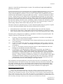
For debugging output, use the -D flag. The argument to this flag consists of one or more of a
series of characters designed to denote a particular level of debugging or object being debugged.
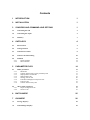
Table 1 contains a list of these characters and the kinds of messages that will be obtained. Any
number of these characters may be specified and in any order. For example, to get messages from
the Land Manager and Land Allocator objects, you would give -D MA as a command line option.
-D option
character
Kinds of debugging message received
P
U
M
A
E
i
c
o
m
n
b
Messages from the Land Parcel objects
Messages from the Land Use objects
Messages from the Land Manager objects
Messages from the Land Allocator object
Messages from the Environment object
Very detailed messages from all objects
Detailed messages from all objects
Messages from the Observer Swarm object
Messages from the Model Swarm object
Messages relating to neighbourhood
Messages relating to bitstrings
Table 1 — List of options to be given as argument to the -D flag, and
their arguments.
For history output, use the -h flag, and give as argument the name of a file to save the history to.
History output records certain properties of objects such as climate, economy, land use, land
Created 2007-02-15
Modified 2007-02-21
Printed 2007-02-21
3 of 69
parcels and land manager each year, in a text format suitable for importing into applications such
as Microsoft Excel.
For specific report output, you need to create a report configuration file indicating what reports
you want made and when you want them to be run. This file is specified using the -R option. Use
the -r option to specify the file you want the report saved to, which if not specified, is
fearlus-report.txt by default. The -a option is used if you are running the model several times, and
rather than creating lots of different report files, you want the reports for all the runs to be stored
in one file. If the -a option is given, then the report will be appended to the file specified with the
-r option if it exists already.
The -d option is used to specify DOS mode output for history and report files. Here, each line is
terminated with Carriage Return, Line Feed, rather than just Carriage Return.
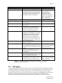
3.3
Summary
For reference purposes, a summary of the command line options that can be given to the model06-8+ELMM0-2 executable is provided in Table 2.
Command line flag
Status
Effect
-a
Optional
-b
Optional
-d
Optional
-D <flags>
-h <file>
-m <mode>
-o <file>
Optional
Optional
Ignored
Optional
-p <file>
-P <file>
Required
Deprecated
-r <file>
Optional
-R <file>
Optional
-s
-S <integer>
-t
-U <file>
Optional
Optional
Ignored
Deprecated
-v
-X {integer | TIME |
DEFAULT}
Ignored
Optional
-Z {integer | TIME}
Optional
Appends to report file rather than creating a
new one if it exists.
Run the model in batch rather than GUI
mode. The default for non-GUI Swarm.
DOS mode output using CR+LF at the end of
each line rather than just CR.
Debugging output.
File to save the history to.
This is a Swarm argument.
Specify a file containing a set of observer
displays you want in GUI mode.
Specify a parameter file for the model.
Specify a land parcel file containing
biophysical properties. This should be done
in the parameter file instead.
File name to save report to if -R option
specified.
Specify the report configuration file to
generate the desired reports.
Set the seed from the current system clock.
Set the seed from the specified argument.
This is a Swarm argument.
Specify a land use file to load land uses in
from. This should be done in the parameter
file instead.
This is a Swarm argument.
Legacy way to set the seed — either specify
an integer or use the word TIME to set the
seed from the system clock, or DEFAULT to
use the Swarm seed.
Specify a second seed to use after
initialisation.
Table 2 — A list of the command line options that may be given to the
model0-6-8+ELMM0-2 executable.
Created 2007-02-15
Modified 2007-02-21
Printed 2007-02-21
4 of 69
4
Ontology
FEARLUS model0-6-8+ELMM0-2 is an abstract agent-based spatially-explicit model of land use
change. It is abstract in the sense that the phenomena simulated are modelled in a manner
designed to mirror the kind of behaviour involved, but are not actually based on any fitted model
of specific objects in the real world. It is agent-based in the sense that it contains objects intended
to represent human decision-makers in the real world: farmers, or (more generally) land
managers, and models these decision-makers individually. It is spatially-explicit in that it has land
parcel objects that are topologically related to each other, decision-making processes that are
bounded in their information sources to a spatial neighbourhood, and outcomes that change the
pattern of certain spatial features (specifically, land use).
Henceforth, entities in the model will be referred to using Title Case to distinguish them from
real-world entities.
4.1
Environment
The Environment consists of a rectangular grid of Land Parcels, and specifies the topological
relationship between those Land Parcels, determining which Land Parcels in the grid have which
other Land Parcels as spatial neighbours. The Topology of the Environment specifies what
happens at the edges of the grid, and the Neighbourhood of the Environment specifies more
generally the size and shape of cells’ neighbourhoods.
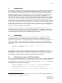
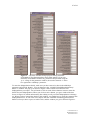
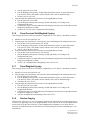
The Topology may be Planar, Toroidal, or Cylindrical. In a Toroidal Topology, edge cells at the
North of the grid ‘wrap-around’ to those at the South (and vice versa), as do those at the East and
West. In a Cylindrical Topology wrap-around occurs in only in the North/South direction
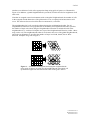
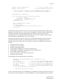
(HorizontalCylindrical) or only in the East/West direction (VerticalCylindrical). Figure 1 shows
the topological effect of wrapping around. In a Planar Topology, no wrap-around of edge cells
takes place.
Figure 1 — Wrapping around a grid of cells in one dimension to form a
cylinder and in two dimensions to form a torus.
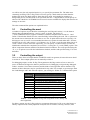
The Neighbourhood Function of the Environment may be von Neumann (squares sharing an edge
are neighbours) or Moore (squares sharing an edge or a corner are neighbours), the two standard
neighbourhoods used in grids of squares, as well as hexagonal or triangular. These last two
Created 2007-02-15
Modified 2007-02-21
Printed 2007-02-21
5 of 69
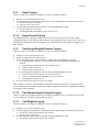
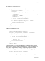
simulate a tessellation of cells of the appropriate shape using grids of squares, as illustrated in
Figure 2. In addition, a global Neighbourhood is provided, in which all cells are neighbours of all
other cells.
Note that in wrapped around environments with a triangular Neighbourhood, the number of cells
in the wrapped around dimension of the grid must be even, or topological inconsistencies will
occur. The software does not check for these inconsistencies, so beware.
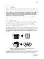
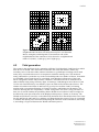
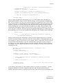
The neighbourhood of a cell can also be adjusted using the neighbourhood radius. For all
Neighbourhood Functions except global and von Neumann, the neighbourhood radius specifies
the number of steps to be taken using the Neighbourhood Function to include all cells in the
neighbourhood (i.e. a radius of 2 implies two steps of the Neighbourhood Function, radius 3 three
steps, and so on). The neighbourhood radius is irrelevant in the case of the global Neighbourhood,
and in the von Neumann, it specifies the number of steps in a North, South, East or West
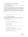
direction. Examples are given in Figure 3.
Figure 2 — Simulation of hexagonal and triangular neighbourhoods
using grids of squares. In each case the neighbourhood of the third cell
up and to the right from the bottom-left corner of the grid is shown.
Created 2007-02-15
Modified 2007-02-21
Printed 2007-02-21
6 of 69
Figure 3 — The effect of neighbourhood radius on various different
Neighbourhood Functions (clockwise from top left: von Neumann,
Moore, triangular, and hexagonal). The outermost cells of the
neighbourhood of the centremost cell is shown for a neighbourhood
radius of 1 (black), 2 (dark grey) and 3 (light grey).
4.2
Yield generation
The Agents in the model survive by generating sufficient Yield from their Land Parcels to enable
them to accrue Wealth. This mirrors the real world to the extent that farmers without any
secondary source of income either continue in business or go bankrupt according to how much
money they can sell their harvest for in comparison with their running costs. The amount of
money obtained for a particular crop in the real world depends on a number of factors. In model06-8+ELMM0-2, three such factors are considered: local Biophysical Properties of the Land
Parcel, and global Climatic and Economic conditions. These three factors are simulated in an
abstract fashion using strings of binary digits, or bitstrings. Land Managers must choose a Land
Use for each Land Parcel they own that they expect to match well with these three factors. The
amount of wealth accrued from a Land Parcel is given by how well the Land Use bitstring
matches with a concatenated bitstring of Climate, Economy, and Biophysical Properties. The
Land Use bitstring has two components, a ‘match’ string and a ‘don’t care’ string. The latter of
these two is used to simulate the possibility that the Wealth accrued from a Land Use might not
be affected by some part of the state of the Biophysical Properties, Climate, or Economy. The
Wealth accrued from a Land Use is also affected by the Break Even Threshold, which is the same
for all Land Parcels and Land Uses, and does not change during the course of a run. It is intended
to simulate the running costs associated with putting the Land Use on the Land Parcel, harvesting
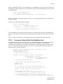
it, and selling it. Figure 4 illustrates the Wealth calculation process.
Created 2007-02-15
Modified 2007-02-21
Printed 2007-02-21
7 of 69
Biophysical Properties
Land Use
Match String
Climate
Economy
0
0
0
1
1
1
0
0
0
0
0
0
1
1
1
0
0
0
1
0
1
1
0
0
1
0
0
0
0
0
0
1
Bitwise Parity
1
1
0
0
1
1
1
1
0
1
1
1
0
0
0
0
LU ‘Don’t
Care’ String
0
0
0
0
0
0
0
0
0
0
0
0
0
1
1
0
Yield String
1
1
1
0
1
1
0
Bitwise OR
1
0
0
1
1
1
1
0
1
Number of 1s in Yield String: 11
Less Break Even Threshold: 8
=> Wealth accrued: 3
Figure 4 — Example Wealth calculation. The Biophysical Properties,
Climate, and Economy are compared with the match string of the Land
Use using the bitwise parity operator, and then the ‘don’t care’ string
applied to the result using a bitwise OR to give the Yield string. The
Wealth accrued is the number of 1s in the Yield string less the Break
Even Threshold.
The number of bits to use for each of the Biophysical Properties, Climate, and Economy are
model parameters, allowing the user to vary the degree to which each of these factors influences
the Wealth accrued from a particular Land Use. The Biophysical Properties vary spatially (in that
each Land Parcel has its own individual Biophysical Properties bitstring), but not temporally (i.e.
this bitstring remains unchanged during the course of a run). The Climate and Economy, by
contrast, do not vary spatially, but may change with each cycle of the model. The bitstrings for
the Land Uses do not change temporally, and do not vary spatially either.
There are two ways in which any of these bitstrings can be set — either using model parameters
to control a stochastic process for setting them, or specifying a file containing the bitstrings to
use. The following discusses the stochastic processes. For Land Uses, the match bitstring is
chosen at random at the beginning of the run, with an equal probability of a 1 or a 0. The ‘don’t
care’ bitstring is also determined during initialisation, using a parameter that specifies, for each
bit, the probability that it will have value 1.
The Climate and Economy are determined initially at random, with an equal probability of either
bit value. Their change over time is determined by a set of parameters with one parameter for
each bit of Climate and Economy specifying the probability that the bit will change in value from
one cycle to the next. A toggle probability of 0 means no change, 1 a certain change. A random
bit value each cycle would be achieved through specifying a toggle probability of 0.5.
The Land Parcel Biophysical Properties are determined at the beginning of the run randomly with
an equal probability of 1 or 0 for each bit. Optionally, a clumping algorithm may be specified,
with the purpose of making neighbouring Land Parcels more similar in their Biophysical
Properties. Model 0-6-8+ELMM0-2 has two clumping algorithms. One (CAVNT3Clumper) is a
cellular automaton which is run on each bit in the Biophysical Properties bitstring in turn. The
transition rule for each bit is to change its value if three or more of its von Neumann neighbours
have the opposite value. The other clumping algorithm (Same10PropClumper) is designed to
maximise the spatial clumpiness of each bit in the Biophysical Properties bitstring whilst
Created 2007-02-15
Modified 2007-02-21
Printed 2007-02-21
8 of 69
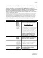
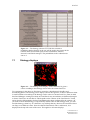
maintaining the same number of 1s and 0s as the initial random setting. The CA clumper takes as
parameter a number of cycles — the more cycles, the more clumped the space. Typically 6 or 7
cycles are sufficient for the CA to converge to a state in which no change is made. The other
clumper takes as a parameter the number of bits in the Biophysical Properties bitstring to clump.
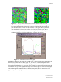
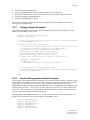
The effect of each clumper is contrasted in Figure 5.
CAVNT3Clumper
Same10PropClumper
Figure 5 — The effect of the two clumpers. Left: Original Biophysical
Properties generated at random, which was used as the initial state for
both clumpers shown. Middle: CAVNT3Clumper after 6 cycles (the 7th
having no effect). Right: Same10PropClumper.
4.3
Land Parcel transfer: ELMM0-2
ELMM stands for Endogenised Land Market Model. ELMM0-1 is discussed in a paper to ESSA
2005 1 . ELMM0-2 consists of a minor upgrade to that model. In ELMM, rather than exchanging
Land Parcels using a fixed price as in FEARLUS, Land Managers bid for their Land Parcels in an
auction.
Land Managers are divided into Subpopulations according to their decision-making processes.
Each Subpopulation is defined by a set of parameters that determine how its member Land
Managers will decide a Land Use for each Land Parcel (see section 4.4) and how they will make
decisions about acquiring Land Parcels. This section pertains to the latter.
The rules for transfer of Land Parcels depend in part on which class of Land Manager is being
used by a Subpopulation. Two such classes are available: PositiveLandManager and
LandManager. Land Managers from the LandManager class who have negative accrued Wealth
are regarded as being bankrupt, and must sell off all their Land Parcels; whilst those from the
PostiveLandManager class must sell off their Land Parcels if they have non-positive Wealth.
Since this is the only restriction on the length of time a Land Manager may spend in the
simulation, a Land Manager is better thought of as representing a farming business or family, than
an individual farmer.
1
Polhill, J. G., Parker, D. C., & Gotts, N. M. (2005) “Introducing land markets to an agent based model of
land use change: A design.” In Troitzsch, K. G. (ed.) Representing Social Reality: Pre-Proceedings of the
Third Conference of the European Social Simulation Association, Koblenz, September 5-9 2005. Koblenz,
Germany: Verlag Dietmar Fölbach. pp. 150-157.
Created 2007-02-15
Modified 2007-02-21
Printed 2007-02-21
9 of 69
All Land Managers in the physical neighbourhood of the Land Parcel being put up for sale are
notified of the availability of the Land Parcel. Each Land Manager has an individual Land Offer
Threshold, which specifies the amount of Wealth they must have before they will consider putting
in a bid for a Land Parcel. Assuming the Land Offer Threshold is exceeded, Land Managers then
proceed to make a bid price for the Land Parcel using a Bidding Strategy. From this set of
potential bids, a Land Parcel Selection Strategy is then used to choose which bids will actually be
made. The total of all bids made must ensure the Land Offer Threshold is still in the Land
Manager’s Account. The Land Allocator is then notified of all the bids made. If a bid is negative
or zero, the Land Allocator ignores it.
The Bidding and Selection Strategies available are listed in the tables below. Note that some of
the Selection Strategies have an issue with potentially making negative bids. These Selection
Strategies should not be used with Bidding Strategies that could make negative bids. For now,
this is just the Discounting Bidding Strategy. Note also that the configuration options for the
Bidding Strategies apply at the Subpopulation level, defining distributions for parameters of
member Land Managers that, once set for an individual Land Manager, do not change.
Bidding Strategy class
Configuration
options
Description
DiscountingBiddingStrategy
rateDist,
rateMin,
rateMax,
rateMean,
rateVar,
windowMin,
windowMax,
lpwgtMin,
lpwgtMax
The bid price, bmp, of Land Manager m for
Parcel p is given by the following formula:
FixedPriceBiddingStrategy
WealthMultipleBiddingStrategy
YieldMultipleBiddingStrategy
priceDist,
priceMin,
priceMax,
priceMean,
priceVar
wealthcDist,
wealthcMin,
wealthcMax,
wealthcMean,
wealthcVar
yieldcDist,
yieldcMin,
yieldcMax,
yieldcMean,
yieldcVar
bmp =
(1 − wm )Pm − wm (y p − T )
rm
where lpwgtMin ≤ wm ≤ lpwgtMax represents
how much Manager m is concerned with the
Parcel’s Yield or their own profit when
making bids, yp is the Yield of Parcel p, T is
the Break Even Threshold, rm is the Land
Manager’s ‘interest rate’ or perceived risk,
sampled from rateDist (‘normal’ or
‘uniform’), and Pm is the mean profit the
Manager has made over the last nm Years,
where windowMin ≤ nm ≤ windowMax
The bid price is a fixed price. Each Land
Manager has their own fixed, constant price
offered, taken from the Subpopulation
distribution priceDist (‘normal’ or ‘uniform’)
The bid price is a constant multiple of the
Land Manager’s account. The coefficient is
taken from the Subpopulation distribution
wealthcDist (‘normal’ or ‘uniform’)
The bid price is a constant multiple of the
most recent Yield of the Land Parcel for sale.
The coefficient is taken from the
Subpopulation distribution yieldcDist
(‘normal’ or ‘uniform’)
Table 3 — The Bidding Strategies available and their configuration
parameters.
Created 2007-02-15
Modified 2007-02-21
Printed 2007-02-21
10 of 69
Selection Strategy class
Description
BuyCheapestSelectionStrategy
Intended to represent an acquisitive strategy for accumulation
of Land, Managers using this strategy bid for the Parcels they
give the least value to. * This is a bit odd, however, as
presumably the bids will not be particular competitive, and if
the Manager did win, the Parcels themselves are not estimated
by the Manager to have much value.
Managers using this strategy bid for the Parcels they value
most highly first.
A random selection of bids is made. Note that some Bidding
Strategies (such as Wealth Multiple) do not discriminate
among Land Parcels. **
BuyDearestSelectionStrategy
RandomSelectionStrategy
Table 4 — The Land Parcel Selection Strategies available.
Once the Land Allocator has received all the bids from existing Land Managers for a Land Parcel,
it generates an in-migrant bid from a randomly chosen Subpopulation, using that Subpopulation’s
In-migrant Offer Price Distribution. The winning bid is then the largest bid made (or if two or
more bids have equal maximum offer price, then a uniform random choice is made among them).
The Land Manager making the winning bid is then the new owner of the Land Parcel. If a
Vickrey auction has been specified, then the price of the exchange is that of the second-highest
bidder. If only one bid is made in a Vickrey auction, or if a first price sealed bid auction is
specified (by setting the vickrey parameter to 0), then the winning bid price is the price of the
exchange.
4.4
Land Use decision making
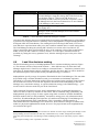
The decision-making process of all Subpopulations has a common underlying structure (Figure
6). The structure consists of three main elements — three different ways in which the Land
Manager might choose a Land Use according to contextual factors — satisfaction, imitation, and
innovation. A fourth element, entirely artefactual, specifies how the Land Use will be decided in
the initialisation phase of the model (usually a Random Strategy is used here).
Subpopulations specify a range of Aspiration Thresholds for their Land Managers. This can either
be specified using a uniform distribution (with given maximum and minimum Aspiration
Threshold), or a normal distribution (with the mean and variance being specified). If the Yield of
the decision Parcel meets or exceeds the Aspiration Threshold of the Land Manager, then the
Manager uses a satisfaction strategy. A typical satisfaction strategy is the Habit Strategy — just
use the Land Use that was used last year on the Land Parcel.
If the Aspiration Threshold is not met, then Land Managers have an individual propensity to
choose a Land Use either by imitation or innovation. This is simulated using a probability, and
Subpopulations specify a range of values (again using either a normal or uniform distribution)
that their members have for this probability. An imitative strategy uses only information about
Land Uses, Wealth and Biophysical Properties of Land Parcels belonging to Land Managers in
the social neighbourhood of the Land Manager. This is intended to simulate transfer of
information between Land Managers on a social basis. Some imitative strategies available in the
model use physical neighbourhoods instead, however. The physical and social neighbourhoods
are contrasted in Figure 7.
*
There is a potential bug here, as negative bids are not filtered out at this stage, meaning the Manager could
end up bidding for more Land Parcels than they could afford to buy. Further, though the bid would be
ignored by the Land Allocator, the Manager would be bidding for Parcels on which they expect to make a
loss!
**
The negative bid bug is also a potential issue here.
Created 2007-02-15
Modified 2007-02-21
Printed 2007-02-21
11 of 69
Start
Yes
Year=0?
Use Initial Strategy
No
Yield >=
Aspiration
Threshold
?
Yes
Use Contentment Strategy
No
Rand() ∈ [0,1]
<= Imitative
Probability
?
Yes
Use Imitative Strategy
No
Use Innovative Strategy
Stop
Figure 6 — Flowchart of underlying structure of the Land Manager
Land Use Decision Algorithm.
O
O M N M M
L
K
K
O
A M M M
E
O
O M A
E
E
E
L
L
E
K
J
P
P
A
A
Z
E
P
O
H
A
Z
Z
J
J
Y
F
X
Y
B
Q
Q
H
F
F
F
G
X
B
B
R
S
H
C
Z
D
S
T
F
G
G
X
U
V
G
I
C
C
W
S
T
V
V
I
I
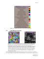
Figure 7 — The social and physical neighbourhoods contrasted. Each
cell in the Environment above is given a letter according to the Land
Manager who owns it. The solid line denotes the boundary of the
physical neighbourhood of Land Manager Z in an Environment with a
von Neumann neighbourhood radius 1. These consist of those Parcels
that share a border with one of the Parcels owned by Z. By contrast, the
social neighbourhood, shown by a grey shading to the included cells,
consists of all Land Parcels owned by Land Managers with Land
Parcels in the physical neighbourhood of Z.
Created 2007-02-15
Modified 2007-02-21
Printed 2007-02-21
12 of 69
There are two other parameters that imitative strategies may or may not use as part of their
algorithm. One is the Neighbourhood Weighting, for which a range of values for Land Managers
is specified at the Subpopulation level. This is intended to represent the degree to which Land
Managers weight information from neighbouring Land Parcels as opposed to their own when
choosing a Land Use to imitate. At a Neighbourhood Weighting of zero, Land Managers only pay
attention to their own Land Parcels, and at a Neighbourhood Weighting of one, Land Managers
give equal weight to all information. The Neighbourhood Weighting otherwise be any positive
floating point number. The one way in which Land Managers’ decision-making processes may be
changed during a simulation run is a legacy provision for the Neighbourhood Weighting to
change. This, somewhat inconveniently, is specified at the global, rather than Subpopulation
level. It specifies the amount to add to the Neighbourhood Weighting of a Land Manager for each
Land Parcel lost, and to subtract from it for each Land Parcel gained.
The other parameter is Neighbourhood Noise, which is determined at the Land Manager level
from a globally specified uniform distribution. (Again, this might be more appropriately specified
at either the Subpopulation level — or even the Environment for that matter.) It is intended to
represent the fact that Land Managers might not always be able to get accurate information about
their neighbours’ Land Parcels. When getting information about neighbouring Parcels’
Biophysical Properties, the Neighbourhood Noise specifies a probability applied to each bit in the
bitstring that a random value will be substituted for the true value of that bit in the bitstring the
Land Manager receives. A Neighbourhood Noise of zero means the Land Manager gets the true
bitstring when querying neighbouring Biophysical Properties, whilst a value of one means the
Land Manager gets an entirely random bitstring.
Innovative strategies do not use neighbourhood information, but involve some other heuristic for
deciding a Land Use to apply from those available. Both imitative and innovative strategies may
involve examining data from earlier cycles. To this end, Subpopulations specify a range of values
for the Memory of Land Managers — which specifies the maximum number of cycles’ Climate,
Economy, Land Use and Yield data the Land Manager may examine when choosing the Land
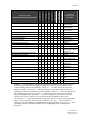
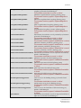
Use. Table 5 compares the list of strategies available for use in model 0-6-8+ELMM0-2. More
detail is given in section 9.
The use of Aspiration Thresholds represents a “satisficing” element to Land Manager behaviour –
i.e. the acceptance of a course of action which is “good enough”, as opposed to a (riskier) attempt
to find the optimum. This satisficing element may be eliminated in a Subpopulation by setting the
minimum threshold higher than the maximum possible Yield — the length of the Land Use
bitstring. In this way, Land Manager decision-making behaviour has some basis in established
theory.
Created 2007-02-15
Modified 2007-02-21
Printed 2007-02-21
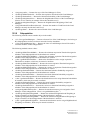
Imitative?
Historical?
Memory?
Phys/Soc
Optimum?
Deterministic?
Nbr wgt?
Nbr noise?
13 of 69
CautiousImitativeOptimumStrategy
Y
Y
N
S
Y
N
N
Y
EccentricSpecialistStrategy
N
Y
N
-
-
-
-
-
FickleStrategy
N
N
N
-
-
-
-
-
HabitStrategy
ImitativeOptimumStrategy
LastNYearsOptimumStrategy
LastYearsOptimumStrategy
MajorityCopyingStrategy
N
Y
N
N
Y
Y
Y
Y
Y
Y
N
N
Y
N
N
S
S
Y
Y
Y
Y
N
Y
Y
N
Y
Y
Y
N
MatchWeightedOptimumStrategy
MatchWeightedRandomStrategy
NeighbouringOptimumStrategy
NoStrategy
N
N
Y
-
N
N
Y
-
N
N
N
-
S
-
Y
N
Y
-
Y
N
-
Y
-
N
-
ParcelCorrectedYieldWeightedCopyingStrategy
ParcelWeightedCopyingStrategy
RandomCopyingStrategy
Y
Y
Y
Y
Y
Y
N
N
N
S
S
S
N
N
N
-
Y
Y
Y
Y
Y
N
RandomStrategy
SimpleCopyingStrategy
N
Y
N
Y
N
N
S
N
N
-
Y
N
SimplePhysicalCopyingStrategy
Y
Y
N
P
N
-
Y
N
StableImitativeOptimumStrategy
StochasticLastYearsOptimumStrategy
StochasticMatchWeightedOptimumStrategy
YieldAverageWeightedTemporalCopyingStrategy
Y
N
N
Y
Y
Y
N
Y
N
N
N
Y
S
S
Y
Y
Y
N
Y
N
N
-
Y
Y
Y
N
YieldRandomOptimumTemporalCopyingStrategy
Y
Y
Y
S
N
-
Y
N
YieldWeightedCopyingStrategy
YieldWeightedTemporalCopyingStrategy
Y
Y
Y
Y
N
Y
S
S
N
N
-
Y
Y
N
N
Strategy name
Land Use
scoring basis /
description
Expected yield with
minimum variance
Random LU first time
retained thereafter
Random LU selected to
use on all Parcels
Retain LU on Parcel
Expected yield
Expected yield
Expected yield
Times LU appears in
neighbourhood
BP match
BP match
BP match
For when a particular
decision algorithm element
won’t be used
BP match * Last yield
BP match
Random if alternative
exists in neighbourhood
Random
Times LU appears in
neighbourhood
Times LU appears in
neighbourhood
Expected yield
Expected yield
BP match
Last N years’ average
yield
Last N years’ average
yield
Last year’s yield
Last N years’ yield
Table 5 — A list of strategies available in model0-6-8+ELMM0-2, their properties and a
brief description. BP refers to Biophysical Properties, and LU refers to Land Use. The
column headings indicate the following: ‘Imitative?’ — Can the strategy be used as an
imitative strategy? ‘Historical?’ — Does the strategy use any data from previous years?
(Meaning it would be unsuitable for an initial strategy) ‘Memory?’ — Does the strategy use
the Land Manager’s memory? ‘Soc/Phys’ — Does an imitative strategy use a social or
physical neighbourhood? ‘Optimum?’ — Does the strategy choose a Land Use with the
highest score? (If not, Land Uses are selected at random weighted by their score.)
‘Deterministic?’ — Does the optimising strategy deal with two or more equally maximum
high scores by choosing consistently (or at random)? ‘Nbr wgt?’ — Does an imitative
strategy use the Land Manager’s neighbourhood weighting property? ‘Nbr noise?’ — Does
an imitative strategy mutate the bitstrings of any neighbouring Parcels’ Biophysical
Properties?
Created 2007-02-15
Modified 2007-02-21
Printed 2007-02-21
14 of 69
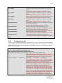
4.5
Schedule
The model contains two schedules, one to run during initialisation, the other to run thereafter. The
main difference between the two (apart from the creation of various objects) is that Land
Managers do not accrue Wealth or exchange Land Parcels during the initialisation schedule, and
they use a different strategy to decide the Land Use.
4.5.1
•
•
•
•
•
•
•
•
•
•
•
Create the Land Parcels, and give them random initial Biophysical Properties.
If a file name is given for the Biophysical Properties and the file exists, then load them from
that file, else if they are to be clumped, then apply the clumper. If a file name for the
Biophysical Properties was given, but the file did not exist, then save them in a file of that
name.
Create the Land Uses, and give them random initial match and ‘don’t care’ bitstrings.
If a file name is given for Land Uses and the file exists, then load them from that file, else if a
file name was specified but the file did not exist, then save them to a file of that name.
Determine the bitstring for the initial Climate, which may involve it being loaded from a file
if a file name was given and the file exists. If a file name was given but the file does not
exist, the Climate bitstrings will be saved to that file each cycle.
Determine the bitstring for the initial Economy, which may involve it being loaded from a file
if a file name was given and the file exists. If a file name was given but the file does not
exist, the Economy bitstrings will be saved to that file each cycle.
Create the Land Managers and assign them to the Land Parcels. Parameters exist that allow
Land Managers to be initially assigned more than one Land Parcel. Essentially they specify
the size of a rectangle of Land Parcels to give to each Land Manager. A whole number of
these rectangles must fit into the Environment grid.
Each Land Manager then determines the initial Land Use of the Land Parcel(s) they own.
Calculate the Yield from each Land Parcel.
If the user has requested a second seed to use after the initialisation schedule (with the -Z
option) then set the random generator to use that seed.
Activate the main schedule.
4.5.2
•
•
•
•
•
•
•
•
•
•
•
Initial schedule
Main schedule
Increment the Year counter. (Each cycle in the model is intended to represent one year.)
Land Managers each choose a Land Use for the Land Parcels they own.
Determine the Climate (and save it to a file if this was specified).
Determine the Economy (and save it to a file if this was specified).
Calculate the Yield.
Land Managers harvest their Yield and accrue Wealth accordingly.
Land Managers with negative Wealth put all their Land Parcels up for sale by informing the
Land Allocator.
The Land Allocator notifies Land Managers neighbouring each Land Parcel for sale.
Neighbouring Land Managers generate bids for each Land Parcel they have been notified of.
The Land Allocator conducts an auction, assigning a (possibly in-migrant) new Land
Manager to the Land Parcels.
Land Managers who sold all their Land Parcels are removed from the schedule.
Created 2007-02-15
Modified 2007-02-21
Printed 2007-02-21
15 of 69
5
Parameter files
In the following section, a bold Courier font is used to indicate text that must appear in the
file as is, whilst an italic Times font is used for text that should be replaced by some appropriate
value. Comments are in a red Arial Narrow font and should not appear in the file.
5.1
Model parameters
Many model parameters take double precision floating point values. Floating point arithmetic is a
means of doing calculations with non-integers and large numbers whilst using a finite number of
bits. In the case of double precision, this is typically an 8-byte word, or 64 bits. Clearly, using this
finite number of bits means that not all numbers between -1.7976931348623157E+308 and
+1.7976931348623157E+308 (see /usr/include/float.h) can be represented accurately. Trivially, in
fact, only 264 or just over 1019 such numbers can maximally be represented. Inevitably, therefore,
floating point arithmetic involves a degree of approximation. Whilst this may be acceptable for
most intents and purposes (double precision giving 15 significant figures of accuracy), there are
some quite simple cases where inaccuracies can occur (try comparing 0.4 + 0.4 + 0.4 – 0.4 – 0.4 –
0.4 with zero, for example). In non-linear applications, such as FEARLUS, where decisions
depend critically on such things as comparisons of floating point numbers with zero, even slight
inaccuracies can have unexpected emergent effects. These inaccuracies can occur simply because
the number in question has a recurring fraction in binary notation (e.g. 0.4 = 0.0110 0110 …), or
because a small number is added to a large number (e.g. 134217728 + 0.00000001 = 134217728).
FEARLUS model 0-6-8+ELMM0-2 does not currently deal effectively with such problems, other
than to issue a warning in one particular case where they are known to have a detectable effect. In
general they should be avoidable by ensuring that any floating point parameters set to nonintegral values uses decimals that are sums of negative powers of two — e.g. 0.5 (2-1), 0.75 (2-1 +
2-2), 0.1875 (2-3 + 2-4), and that the model is not left running for a huge number of Years (which
makes the sum of large and small numbers more likely to be an issue).
5.1.1
Model file
The model file is the main parameter file, and it is this that should be supplied as argument to the
–p flag on the command line. The ‘environmentType’ parameter needs a little explanation. The
value given is a string consisting of a Topology and Neighbourhood Function, separated by a
minus sign. The Topology may be one of ‘Global’, ‘Planar’, ‘HorizontalCylindrical’,
‘VerticalCylindrical’, or ‘Toroidal’. The Neighbourhood Function may be one of
‘TriangularVonNeumann’, ‘VonNeumann’, ‘HexagonalParallelogram’, ‘Moore’, or ‘Global’.
Thus examples for this parameter value are such strings as ‘Planar-VonNeumann’, ‘ToroidalHexagonalParallelogram’, or ‘HorizontalCylindrical-Moore’. The ‘Global’ Topology and
‘Global’ Neighbourhood are intended to be used exclusively together, in the environment type
‘Global-Global’. Combining the Global Topology or Neighbourhood with any other
Neighbourhood or Topology is an error, but will not cause the model to fail.
The ‘clumping’ parameter also needs some explanation. The value to use for this parameter is a
string in which the type of clumper and any parameters it needs are given. The format of this
string is clumper:param1=value1;param2=value2;…;paramN=valueN. Two clumpers are
available in model0-6-8+ELMM0-2: ‘CAVNT3Clumper’, and ‘Same10PropClumper’, described
earlier in this document. The ‘CAVNT3Clumper’ has one parameter ‘Cycles’ which should
always be specified, and tells the clumper how many cycles of the CA to do. The
‘Same10PropClumper’ has one parameter ‘bitsToClump’ which specifies how many bits of the
Biophysical Properties bitstring should be clumped (the CA clumper does not have such an
option). This is an optional parameter, as by default the ‘Same10PropClumper’ will clump all
bits. Examples of settings for the ‘clumping’ parameter are ‘CAVNT3Clumper:Cycles=6’,
‘Same10PropClumper’, or ‘Same10PropClumper:bitsToClump=1’. If no clumping is required,
then the string ‘None’ should be used.
Created 2007-02-15
Modified 2007-02-21
Printed 2007-02-21
16 of 69
The model file format is given below:
@begin
environmentType
neighbourhoodRadius
climateBSSize
economyBSSize
landParcelBSSize
nLandUse
pLandUseDontCare
clumping
envXSize
envYSize
landParcelFile
useLandParcelFile
landUseFile
useLandUseFile
economyFile
useEconomyFile
economyToggleProbFile
climateFile
useClimateFile
climateToggleProbFile
maxYear
infiniteTime
Environment type string, as described in the main text
Neighbourhood radius (integer)
The neighbourhoodRadius must be less than half of both
envXSize and envYSize. This is not validated, but will result in
invalid neighbourhoods being computed.
Number of bits to use for the Climate bitstring (integer)
Number of bits to use for the Economy bitstring (integer)
Number of bits to use for the Land Parcel Biophysical
Properties bitstring (integer)
The length of the Land Use bitstring is always the sum of the
Climate, Economy, and Biophysical Properties bitstring lengths
Number of Land Uses (integer)
Probability of a 1 in the ‘Don’t care’ bitstring of any Land
Use
Clumping algorithm to use and any parameter settings as
described in the main text
Number of horizontal cells to use in the Environment grid
(Integer)
Number of vertical cells to use in the Environment grid
(Integer)
File to use to load (or save) Biophysical Properties from
The useLandParcelFile parameter must be set to 1 for this file to
be used. If the file already exists (and useLandParcelFile = 1),
then the Biophysical Properties will be loaded from it. If not, then
they will be saved to it.
Flag indicating whether or not to use the landParcelFile
File to use to load (or save) Land Use bitstrings from
Flag indicating whether or not to use the landUseFile
The useLandUseFile and landUseFile parameters are linked in
the same way as the useLandParcelFile and landParcelFile
parameters, and the same behaviour relative to the existence of
the file also applies here.
File to use to load (or save) Economy bitstrings from
If the file contains fewer Years’ worth of Economy bitstrings than
are used in the model run, then once the bitstrings in the file are
used up random bitstrings are generated using the toggle
probabilities.
Flag indicating whether or not to use the economyFile
Again, the file won’t be used unless the corresponding ‘use…’
parameter = 1, and the load/save behaviour is the same.
File to load the Economy toggle probabilities from
File to use to load (or save) Climate bitstrings from
Flag indicating whether or not to use the climateFile
climateFile behaviour is just the same as economyFile behaviour.
File to load the Climate toggle probabilities from
Number of iterations of annual cycle
Essential for batch runs! The number entered here should
actually be one more than the maximum Year you want reported.
Flag indicating whether or not to run indefinitely (1 to run
indefinitely, 0 to use maxYear)
Created 2007-02-15
Modified 2007-02-21
Printed 2007-02-21
17 of 69
nSubPops
subPopFile
strategyChangeUnit
neighbourNoiseMax
neighbourNoiseMin
breakEvenThreshold
vickrey
nInitXParcels
nInitYParcels
dumpHistory
maxHistoryLength
Must be 0 for batch runs!
Number of subpopulations in this run (integer)
File to load subpopulation contest data from
Amount by which to update all Land Managers’
Neighbourhood Weighting (floating point)
Maximum probability of corrupting each bit in a
neighbouring Parcel Biophysical Properties query to
endow Land Managers with (floating point)
Corresponding minimum probability (floating point)
Amount to subtract from Yield to get Wealth accrued to
Land Manager from one Land Parcel (floating point)
Flag indicating whether to use a Vickrey auction or a firstprice sealed bid auction (1 to use Vickrey, 0 to use firstprice sealed bid)
Number of initial horizontal Land Parcels to endow the
Land Managers created at the beginning of the run with
(integer)
envXSize must be an integer multiple of this parameter value
Number of initial vertical Land Parcels to endow the Land
Managers created at the beginning of the run with
(integer)
envYSize must be an integer multiple of this parameter value
Flag indicating whether or not to save off the history
gathered so far into an intermediate file (to save memory
and size of each history file) (1 to use intermediate files, 0
to save everything to one big file at the end of the run)
How many Years’ data to save in each intermediate history
file (integer)
To use these history parameters, the -h option must be specified
on the command line.
@end
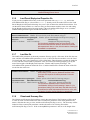
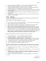
5.1.2
Climate and Economy toggle probability files
The Climate and Economy toggle probability files both have the same format. They are used to
specify the probability of changing value each Year for each bit of their respective bitstrings. Zero
length Climate and Economy bitstrings are permitted in model0-6-8+ELMM0-2, but
unfortunately you still have to provide a toggle probability file (which consists of a single line
saying “NumberOfElements: 0”). The format is given below:
NumberOfElements: Number of bits for which probabilities are provided (integer)
The number entered here must correspond to the model file
parameters climateBSSize or economyBSSize according to
which of the Climate or Economy this file is for.
d Probability this bit will flip each Year (floating point)
The above line should appear the number of times indicated by
the NumberOfElements entry.
5.1.3
Subpopulation contest file
The Subpopulation contest file specifies which Subpopulations will be competing for land
ownership in this run of the model.
Created 2007-02-15
Modified 2007-02-21
Printed 2007-02-21
18 of 69
NumberOfSubPopulations: Number of Subpopulations in the contest (integer)
The number entered here must correspond to the model file
parameter nSubPops.
SubPopulationFile Subpopulation file number (integer): Subpopulation file name
The above line should appear the number of times indicated by
the NumberOfSubPopulations entry. The Subpopulation file
number should start at 1 on the first SubPopulationFile line and
increase in steps of 1.
5.1.4
Subpopulation file
The Subpopulation file contains details of the ranges of parameters that will be assigned to Land
Managers belonging to this Subpopulation. Some ranges of parameters can be specified using a
normal or a uniform distribution. In each of these cases, there will be a parameter called ‘…Dist’
that specifies which to use (the value for which should be either ‘normal’ or ‘uniform’). If the
‘…Dist’ parameter is ‘uniform’, then the range of values is specified using the corresponding
‘…Min’ and ‘…Max’ parameters, otherwise, the ‘…Mean’ and ‘…Var’ parameters should be
used. The file also contains a pointer to the strategy selector file, which determines which
strategies member Land Managers will use for contentment, imitation, innovation or initially.
The ‘biddingStrategyConfig’ parameter needs some explanation. This is given as a semicolonseparated string of Bidding Strategy configuration parameter settings, similarly to the clumper in
the main model file: param1=value1;param2=value2;…;paramN=valueN. Refer to Table 3 for
more information on these parameters. An example biddingStrategyConfig string for a
FixedPriceBiddingStrategy would be:
priceDist=normal;priceMean=1.0;priceVar=0.0
@begin
label
colour
probability
landMgrClass
strategySelectorFile
memorySizeMin
memorySizeMax
String containing a unique name for this Subpopulation
The label is optional — a label will be generated automatically if
none is specified. The label is of most use in GUI mode to tell the
Subpopulations apart on the graphs.
A colour to use for this Subpopulation (integer)
The colour is also optional, and only relevant in GUI mode.
Colours are preset in a colourmap, and they are indexed by this
integer, which should be a positive integer. Colours will be
automatically assigned to Subpopulations if not specified here.
The only reason to specify the colour is for consistency across a
number of runs.
The probability that any newly created Land Manager will
belong to this Subpopulation (floating point)
Which class to use to represent the Land Managers.
This parameter should either be ‘LandManager’ or
‘PositiveLandManager’, depending on the Land Parcel transfer
mechanism required.
The name of a file to get the strategies for this
Subpopulation from
The minimum number of Years a member of this
Subpopulation will be able to recall Climate, Economy,
Yield and Land Use data for. (integer)
The maximum number of Years… (integer)
Created 2007-02-15
Modified 2007-02-21
Printed 2007-02-21
19 of 69
Distribution from which to set the neighbourhood
weighting of member Land Managers
This parameter should either be ‘normal’ or ‘uniform’.
neighbourWeightMin
Minimum neighbourhood weighting (floating point)
This parameter should only appear if ‘neighbourWeightDist’ is
‘uniform’.
neighbourWeightMax
Maximum neighbourhood weighting (floating point)
This parameter should only appear if ‘neighbourWeightDist’ is
‘uniform’.
neighbourWeightMean
Mean neighbourhood weighting (floating point)
This parameter should only appear if ‘neighbourWeightDist’ is
‘normal’.
neighbourWeightVar
Neighbourhood weighting variance (floating point)
This parameter should only appear if ‘neighbourWeightDist’ is
‘normal’.
imitateProbDist
Distribution from which to set the probability of imitation
of member Land Managers
This parameter should either be ‘normal’ or ‘uniform’.
imitateProbMin
Minimum imitation probability (floating point)
This parameter should only appear if ‘imitateProbDist’ is ‘uniform’.
imitateProbMax
Maximum imitation probability (floating point)
This parameter should only appear if ‘imitateProbDist’ is ‘uniform’.
imitateProbMean
Mean imitation probability (floating point)
This parameter should only appear if ‘imitateProbDist’ is ‘normal’.
imitateProbVar
Imitation probability variance (floating point)
This parameter should only appear if ‘imitateProbDist’ is ‘normal’.
habitImitateThresholdDist Distribution from which to set the aspiration threshold of
member Land Managers
This parameter should either be ‘normal’ or ‘uniform’.
habitImitateThresholdMin Minimum aspiration threshold (floating point)
This parameter should only appear if ‘habitImitateThresholdDist’
is ‘uniform’.
habitImitateThresholdMax Maximum aspiration threshold (floating point)
This parameter should only appear if ‘habitImitateThresholdDist’
is ‘uniform’.
habitImitateThresholdMean Mean aspiration threshold (floating point)
This parameter should only appear if ‘habitImitateThresholdDist’
is ‘normal’.
habitImitateThresholdVar Aspiration threshold variance (floating point)
This parameter should only appear if ‘habitImitateThresholdDist’
is ‘normal’.
biddingStrategyClass
Class to use for the Bidding Strategy of member Land
Managers
This parameter should either be ‘normal’ or ‘uniform’.
biddingStrategyConfig
Configuration string for the Bidding Strategy
This parameter should only appear if ‘habitImitateThresholdDist’
is ‘uniform’.
selectionStrategyClass
Class to use for the Land Parcel Selection Strategy of
member Land Managers
This parameter should only appear if ‘habitImitateThresholdDist’
is ‘uniform’.
priceDist
Distribution from which to set the in-migrant Land Parcel
Offer Price of member Land Managers
neighbourWeightDist
Created 2007-02-15
Modified 2007-02-21
Printed 2007-02-21
20 of 69
priceMin
priceMax
priceMean
priceVar
landOfferDist
landOfferMin
landOfferMax
landOfferMean
landOfferVar
This parameter should either be ‘normal’ or ‘uniform’.
Minimum in-migrant Land Parcel Offer Price (floating
point)
This parameter should only appear if ‘priceDIst’ is ‘uniform’.
Maximum in-migrant Land Parcel Offer Price (floating
point)
This parameter should only appear if ‘priceDist’ is ‘uniform’.
Mean in-migrant Land Parcel Offer Price (floating point)
This parameter should only appear if ‘priceDist’ is ‘normal’.
In-migrant Land Parcel Offer Price variance (floating
point)
This parameter should only appear if ‘priceDist’ is ‘normal’.
Distribution from which to set the Land Offer Threshold of
member Land Managers
This parameter should either be ‘normal’ or ‘uniform’.
Minimum Land Offer Threshold (floating point)
This parameter should only appear if ‘landOfferDist’ is ‘uniform’.
Maximum Land Offer Threshold (floating point)
This parameter should only appear if ‘landOfferDist’ is ‘uniform’.
Mean Land Offer Threshold (floating point)
This parameter should only appear if ‘landOfferDist’ is ‘normal’.
Aspiration Land Offer Threshold (floating point)
This parameter should only appear if ‘landOfferDist’ is ‘normal’.
@end
5.1.5
Strategy selector file
The strategy selector file contains a list of strategies to use for each element in the Land Manager
Decision Algorithm, and the probability that the strategy will be selected. This allows, if required,
Subpopulations to consist of Land Managers using different strategies for different elements in
the Decision Algorithm.
NumberOfStrategyClasses: Number of strategies appearing in this file (integer)
Class AboveThresholdProbability \
BelowThresholdNonImitativeProbability \
BelowThresholdImitativeProbability InitialProbability
The above headings should all appear on one line. The file is
designed to be readable in a spreadsheet package, so separating
the headings with tabs is a good idea, though not necessary.
Name of strategy
Probability1 Probability2 Probability3 Probability4
The strategy names are given in Table 5. The first probability is
the probability the strategy will be assigned as the contentment
strategy of a Land Manager. The second probability is the
probability it will be assigned as the innovative strategy. The third
is for the imitative strategy, and the fourth the initial strategy
(typically ‘RandomStrategy’). Where the distributions of
parameters in the corresponding Subpopulation file have been
appropriately set, ‘NoStrategy’ should be used with probability 1
to generate an error message if the Land Manager attempts to
use it. Thus, for example, if the minimum aspiration threshold is
greater than the maximum possible yield, then NoStrategy should
be in here with Probability1 replaced with 1.0, and 0.0 for
Probability2-4. The number of strategy lines in the file should
Created 2007-02-15
Modified 2007-02-21
Printed 2007-02-21
21 of 69
correspond to the number entered for
‘NumberOfStrategyClasses’ above.
5.1.6
Land Parcel Biophysical Properties file
If you provide a landParcelFile entry in the main parameter file (say, file1.lp), and set the
useLandParcelFile flag to 1, then unless file1.lp already exists, the model will save the Land
Parcel Biophysical Properties bitstrings for you to a file of that name with the format below. You
can then have them loaded in to a later run using an Environment with the same size and setting
for the Biophysical Properties bitstring length, if the useLandParcelFile flag is set to 1, and the
landParcelFile parameter again contains the filename file1.lp.
EnvironmentXSize: Number of horizontal cells in the Environment (integer)
EnvironmentYSize: Number of vertical cells in the Environment (integer)
LandParcelBitStringLength: Number of bits in the Biophysical Properties (integer)
XCoord
YCoord
BitString
Cell X co-ordinate
Cell Y co-ordinate
Biophysical Properties bitstring
The line above is repeated for each cell (Land Parcel) in the
Environment. Note that when the file is saved from the model,
tabs separate each item on a line, with the intention of making the
file readable in a spreadsheet.
5.1.7
Land Use file
The landUseFile parameter in the main parameter file may specify a file name. If the file does not
exist, and the useLandParcelFile parameter is set to 1, this will cause the model to save the Land
Use match and ‘don’t care’ bitstrings in a file of that name. These bitstrings can then be loaded in
to a run with the same nLandUse parameter value, and Land Use bitstring length (given by the
sum of the lengths of the Biophysical Properties, Climate and Economy bitstrings). The
useLandParcelFile parameter should be set to 1, and the landUseFile contain the name of the file
saved from the earlier run.
NumberOfLandUses: Number of Land Uses (integer)
When loading in Land Uses, the ‘NumberOfLandUses’ value
given here must equal the nLandUse parameter in the main
model file.
LandUseBitStringLength: Number of bits in the Land Use bitstring (integer)
LandUseIndex
MatchBitString
DontCareBitString
LU number (integer) Match bitstring of Land Use
‘don’t care’ bitstring of Land Use
The line above is repeated for each Land Use, with the
‘LandUseIndex’ starting at 0 and increasing in steps of 1 (it is
ignored when loading in the Land Uses). Note that when the file
is saved from the model, tabs separate each item on a line, with
the intention of making the file readable in a spreadsheet.
5.1.8
Climate and Economy files
The Climate and Economy files both have exactly the same format. The Economy will be saved
to a file for each Year the model runs if the economyFile parameter in the main parameter file
names a file that does not yet exist, and the useEconomyFile flag is set to 1. The Economy will be
loaded in if the economyFile parameter contains the name of an existing file and the
useEconomyFile flag is set to 1. If the economyBSSize parameter is not set to the length of the
Created 2007-02-15
Modified 2007-02-21
Printed 2007-02-21
22 of 69
bitstrings in the file, then the model will generate an error message. The same applies to the
Climate, and the climateBSSize, climateFile and useClimateFile parameters.
The format of the file is simple: one line per Year, with each line having the required bitstring. If
the run is loading in bitstrings from a file, and the file ends before the run’s termination Year,
then subsequent Climates/Economies will be generated using the toggle probabilities. Note that
these probabilities must be set, even if it is not expected they will be needed.
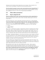
5.2
Observation parameters
5.2.1
Report configuration file
The report configuration file is used to specify the reports that are required as output from the
model, any options for those reports, and in what Years the reports are to be made. Reports are
discussed in more detail in section 0, where a table of currently available reports is also to be
found (Table 7).
The format of this file is a series of statements separated by white space in a simple language.
Every report configuration file must finish with the word “End”. The simplest configuration file
consists solely of this word, and will call every report each Year. Optionally, the first statement in
the file can be one saying “DefaultYearsToReport: Year list” (without the quotes). A
Year list is a comma-separated list of terms, where each term may be one of the following:
• integer1
• integer2-integer3
• Every integer4
Here, integer1 is greater than or equal to 0, and specifies a fixed Year in which the report will be
made. Next, integer2 is also greater than or equal to 0, and integer3 is greater than integer2, and
they together specify an inclusive fixed range of Years in which to report. Finally, integer4 is a
repeat interval. The report will be called in Year 0 (the initialisation Year), and then in intervals
of integer4 thereafter. There must be no white space between a term and a comma following it.
For example: “DefaultYearsToReport: 7, 9, Every 20, 70-80, Every 99, 199” would, in a run with
the maxYear parameter set to 200, stipulate the default that reports would be called in Years 0, 7,
9, 20, 40, 60, 70, 71, 72, 73, 74, 75, 76, 77, 78, 79, 80, 99, 100, 120, 140, 160, 180, 198, and 199.
Note that Year 200 is not reported on; the maxYear parameter specifies the Year to stop the
simulation, and reports are never issued for that Year.
The next simplest report configuration file besides that consisting only of the word “End” is one
consisting of a DefaultYearsToReport statement followed by the word “End”. For example, a file
containing “DefaultYearsToReport: 200 End” would specify (in a run with maxYear more than or
equal to 201) that all reports were to be written in Year 200.
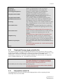
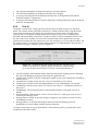
More typically, however, only a few of the available reports in Table 7 will be required.
Following the optional DefaultYearsToReport statement, a series of statements should be
specified for each report required. Each such statement consists of the name of the report class (as
given in Table 7), followed (if required) by a list of options, followed (if DefaultYearsToReport
have not been specified and the report is not required every Year, or the defaults are to be overridden for this report) by a Year list. An option list is preceded by the term “Options:” if it
appears, and a Year list by the term “YearsToReport:”.
Created 2007-02-15
Modified 2007-02-21
Printed 2007-02-21
23 of 69
Report configuration file
What it does
End
DefaultYearsToReport: Every 10
End
ParcelSubPopReport
YearsToReport: 200
End
DefaultYearsToReport: Every 1
ClimateBitStringReport
EconomyBitStringReport
ClumpinessReport
Options: Histo
YearsToReport: 0
ParcelSubPopReport
YearsToReport: 200
End
Every report, every Year.
Every report, every 10 Years.
ParcelSubPopReport
in Year 200 only.
ClimateBitStringReport and
EconomyBitStringReport every Year,
ClumpinessReport
showing a histogram
in Year 0 only,
and ParcelSubPopReport
in Year 200 only.
Table 6 — Some example report configuration files. Note that spacing
in the file is irrelevant so long as white space of some kind appears
where it appears in the example — the layout shown here is to improve
readability.
An option list is a comma-separated list of option terms specifying the value of each option.
Options come in two forms, variables and flags. The following shows the format for setting them:
•
•
•
variable1=value
flag1
Noflag2
Here, variable1 is set to the specified value, flag1 is set to “True” and flag2 is set to “False”.
When specifying a list of options, there must be no white space between an option term and any
following comma. Any report having options will have default values for them. In model0-68+ELMM0-2 the only report with any option is the ClumpinessReport, which has a Histo flag.
Some examples are given in Table 6.
5.2.2
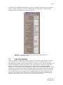
Observer file
The observer file specifies which displays are required when the model is being run in GUI mode.
The default is to show all displays, which, unless you have an unusually large screen, is likely to
lead to rather a lot of clutter. Examples of each of the displays are given in section 7 which
discusses GUI mode in more detail. The format of the observer file is given below:
@begin
showStrategyColourKey
showUseRaster
showLPBitStringRaster
showLPBitStringDiffs
boolean
The Strategy raster shows a colour on each Land Parcel for the
Strategy used to determine its Land Use. This display shows the
key to those colours. The value 1 means the raster should be
shown the value 0 that it should not.
boolean
Show the Land Parcels coloured by their current Land Use
boolean
Show a raster containing a display of the setting of a particular bit
in the Biophysical Properties of the Land Parcels. You can cycle
through the bit displayed by left and right clicking in the raster.
boolean
Created 2007-02-15
Modified 2007-02-21
Printed 2007-02-21
24 of 69
If the Land Use raster is displayed, setting this flag to 1 will show
on the border between each von Neumann neighbouring Land
Parcel a grey line whose shade indicates the number of bits that
match between that pair of Land Parcels’ Biophysical Properties.
Black is no match, white is all matching.
showManagerRaster
boolean
Show the Land Parcels coloured by the Land Managers owning
them.
showSubPopRaster
boolean
Show the Land Parcels coloured by the Subpopulation of the
Land Managers owning them.
showStrategyRaster
boolean
Show the Land Parcels coloured by the Strategy used to choose
their Land Use.
showUseChangeRaster
boolean
Show the Land Parcels in shades of grey according to the relative
number of times their Land Uses have been changed (black =
least, white = most).
showManagerChangeRaster
boolean
Show the Land Parcels in shades of grey according to the relative
number of times their Land Managers have been changed (black
= least, white = most).
showPriceRankRaster
boolean
Show the Land Parcels in shades of grey according to the relative
most recent price (black = cheapest, white = most expensive,
yellow = not sold yet).
showAveragePriceRankRaster boolean
Show the Land Parcels in shades of grey according to the relative
average price at which they have been sold (black = cheapest,
white = most expensive, yellow = not sold yet).
showTotalPriceRankRaster boolean
Show the Land Parcels in shades of grey according to the relative
total price of all times they have been sold (black = cheapest,
white = most expensive).
showParcelsOwnedGraph
boolean
Show a time series graph of the total number of Land Parcels
owned by members of each Subpopulation. If there is only one
Subpopulation, show the mean, minimum and maximum over all
Land Managers.
showYieldGraph
boolean
Show a time series graph of the mean, minimum and maximum
Yield from the Land Parcels.
showPopulationGraph
boolean
Show a time series graph of the number of Land Managers in
each Subpopulation.
showUseGraph
boolean
Show a time series graph of the number of Land Parcels
assigned to each Land Use.
showWealthGraph
boolean
Show a time series graph of the mean Wealth accumulated by
members of each Subpopulation. If there is only one
Subpopulation, show the mean, minimum and maximum over all
Land Managers.
showManagersDist
boolean
Created 2007-02-15
Modified 2007-02-21
Printed 2007-02-21
25 of 69
showAgeGraph
showPriceGraph
showNewBidGraph
showBidGraph
showNWeightDist
showThresholdDist
showImitProbDist
nHistogramBins
zoomSize
displayFrequency
saveDumpedHistory
blackAndWhite
Show a distribution of the number of Land Managers owning
each possible number of Land Parcels.
boolean
Show a time series graph of the mean Age (in Years) of members
of each Subpopulation. If there is only one Subpopulation, show
the mean, minimum and maximum over all Land Managers.
boolean
Show a time series graph of the mean, minimum and maximum
price at which Land Parcels have been sold.
boolean
Show a time series graph of the mean bids offered by in-migrant
members of each Subpopulation for each Land Parcel.
boolean
Show a time series graph of the mean bids offered by non-inmigrant members of each Subpopulation for each Land Parcel.
boolean
Show (if appropriate) a distribution of the Neighbourhood
Weighting over members of each Subpopulation — so, one graph
for each Subpopulation with parameters set to allow this to vary.
boolean
As showNWeightDist, but for the Aspiration Threshold.
boolean
As showNWeightDist, but for the Imitation Probability.
integer
Number of bins to use in the distribution graphs except that
displayed if showManagersDist = 1. (So, all graphs have the
same number of bins…)
integer
How many units of 250 pixels to make the rasters. This multiple
of 250 pixels will determine the number of pixels to use for the
larger dimension of the Environment. So, if the zoomSize is 2 and
the Environment has 10 horizontal Land Parcels and 4 vertical,
then all raster displays will be 500 pixels across by 200 pixels
down.
integer
How often to update the display of all rasters and graphs.
boolean
Set to 1 to use history output in GUI mode.
boolean
Create grey-shaded GUIs rather than colour where possible.
@end
6
Batch mode
As mentioned in section 3, to run FEARLUS in batch mode, give the -b flag to the command line.
If FEARLUS has been compiled against Swarm libraries configured without a GUI, then batch
mode is the default. Any debugging output specified with the -D flag will be sent to stdout, along
with standard messages that can’t be optionally made to disappear showing (among other things)
when each Year is started. You should give at least one of -D, -h, or the -R and -r flags to get
some output from the model, otherwise there is little point in running it. If you are not giving the
-D flag, then stdout should be redirected to /dev/null to discard it, particularly if you are running
the process in the background (this works on both Unix and Cygwin — see below for an example
command). Successful termination is indicated by a 0 exit status. More on the output options can
Created 2007-02-15
Modified 2007-02-21
Printed 2007-02-21
26 of 69
be found in section 0. The -p flag should also be used to specify the model parameters for the run,
and unless the run is being used to test the model, the -s flag should be given to specify an
arbitrary seed (or -S with a specific seed).
Bear in mind that using the -s flag to vary the seed could result in duplicate seeds being used
(though this is not very likely), as the -s flag generates a seed from the system clock and process
ID. There are two ways of approaching this: either check the output (all the output options give
the seed used) and discard duplicates, or prepare a list of unique seeds in advance for each
sequence of runs, and cycle through them using the -S option. The latter option would require
some sort of script to start off each run.
Another point to note for series of runs is that the -a flag will append any reports specified with
the -R option to the file specified with the -r option. For large numbers of runs, this can prevent
directories being cluttered with large numbers of report files.
A typical command to run the model in batch mode would look like this:
/full/path/to/model0-6-8+ELMM0-2 -p MyParams.model -R
MyReports.cfg -r MyReportOutputFile -s -a > /dev/null
One point to note from this example is that the model is being run from the directory containing
all the parameter files. If this is not done, then all filenames in parameter files should use full
paths. This latter approach could be useful in maintaining a database of parameter file settings
using the filesystem, but would impact the portability of the parameter files.
7
GUI mode
GUI mode is typically used for exploratory runs of the model, and for generating pictures for
diagrams. A large number of displays are possible in GUI mode, and it is suggested that an
observer file (section 5.2.2) be used to select the displays required. These, and any options for
setting them, are all illustrated in the ensuing subsections.
First, however, it is worth noting that the GUI can be used (to a certain extent) to enter parameters
for the model and for the observer. This is not strictly recommended, as no record of the
parameters will be saved unless you are using reporting or history output. It also has to be said
that the GUI entry of some of the Subpopulation parameters in particular should be regarded as
alpha release at best * . Further, there is no ability to enter the toggle probabilities for the Climate
and Economy, so at the very least you will have to create these files (even if you have zero-length
bitstrings for them!). Thus, although, in section 3 the -p option was specified as mandatory,
strictly speaking, it is not, and the model can be run without any command-line options. This,
however, is not recommended practice.
When the model is first started, three windows appear, Figure 8 illustrating the contents of these
windows when no command-line arguments are given. In this case, you should enter values for all
parameters (making sure you press return after each entry) except climateToggleProbs,
economyToggleProbs, subPops, and panel. Some parameters are optional — in particular
landParcelFile, landUseFile, climateFile and economyFile need not be entered if their
corresponding use… flags are set to 0. You should also be able to get away without entering the
subPopFile, as the GUI lets you enter Subpopulation details manually. If you have specified a
parameter file with the -p option, then you can use the GUI to make changes to the parameters if
you want to, before pressing ‘Next’ or ‘Start’ to begin running the model. You can also enter
values for the seed for the run, and, if required, the seed to use after initialisation. You cannot
change the parameters once the run has started.
*
… and is unlikely ever to be beta.
Created 2007-02-15
Modified 2007-02-21
Printed 2007-02-21
27 of 69
Figure 8 — The three windows that pop up on starting model0-68+ELMM0-2. The illustration here shows what appears if you start
model0-6-8+ELMM0-2 without any parameter file specified using the
-p or -o flags. In the parameter window, the user has entered ‘2’ in the
box against the ‘nSubPops’ parameter.
To enter the Subpopulation details, make sure you have entered a value in the nSubPops
parameter and pressed ‘Return’. You can then press the ‘clickMeToGetSubPopulationArray’
button. A window will pop up as shown in Figure 9 that contains one button for each
Subpopulation you require. You will need to click on each of these buttons in turn to enter the
details for each Subpopulation. When you click on such a button, you get a window like that
shown in Figure 10 (which unfortunately has nothing to tell you which Subpopulation it belongs
to). When you have entered the details in this window, you further have to enter the strategies this
Subpopulation uses. It will come as no surprise that the ‘clickMeToGetStrategySelectorGUI’
button is what you have to press to achieve this, and the window you get is shown in Figure 11.
Created 2007-02-15
Modified 2007-02-21
Printed 2007-02-21
28 of 69
Figure 9 — The Subpopulation array window that appears when you
click on the ‘clickMeToGetSubPopulationArray’ button on the
Parameter window. There is one button from 1 to nSubPops as entered
on the Parameter window.
Figure 10 — The Subpopulation parameter entry window.
To be absolutely clear, you have to get the Subpopulation and Strategy selector GUIs for each
Subpopulation in separate windows, and enter all the details. If you are intending to use several
Subpopulations, that’s a lot of windows, and a lot of entering. If you are entering all that data on
the GUI, then you might as well be putting it in files using a text editor, and then you can use it
again in a later run.
One other point worth mentioning about GUI mode is that the maxYear parameter behaves
differently in GUI mode than it does in batch mode. In batch mode, maxYear is necessary to
specify when the simulation should terminate. In GUI mode, however, this is not required, as the
‘Quit’ button is there for you to exit at any time. If the infiniteTime parameter is 0, then the
simulation will pause at maxYear. You can then click ‘Next’ or ‘Start’ to keep running, or ‘Quit’
to exit.
Created 2007-02-15
Modified 2007-02-21
Printed 2007-02-21
29 of 69
Figure 11 — The Strategy selector GUI. Each box contains a
probability that the Strategy in the row will be used in the context in the
column, which (from left to right) are the contentment, imitative,
innovative and initial strategies. The probabilities in the columns must
sum to 1.
7.1
Strategy displays
Figure 12 — The Strategy raster display. Each Land Parcel is given a
colour according to the Strategy used to select its current Land Use.
Two parameters in the observer file relate to strategies: showStrategyColourKey and
showStrategyRaster. The Strategy raster display is shown in Figure 12. It shows a different colour
in each Land Parcel according to the Strategy used to select its current Land Use. (Bear in mind
that Land Managers owning more than one Land Parcel may nevertheless use different Strategies
to choose Land Uses on each Parcel. This depends on the contexts of the Land Parcels’ Yields,
and on how the Subpopulation for that Land Manager has been configured for the contexts.) If
you want to know what Strategy is represented by which colour on the Strategy raster, you will
need the Strategy colour key. It is therefore very unlikely that any observer file would have these
two flags set to different values. Note also that the Land Parcel with co-ordinate (0, 0) is
displayed at the top-left corner of the raster. This applies to all raster displays.
Created 2007-02-15
Modified 2007-02-21
Printed 2007-02-21
30 of 69
Figure 13 — The key to the colours shown on the Strategy raster.
7.2
Land Manager displays
Figure 14 — The Land Manager (left hand side) and Land Manager change (right
hand side) rasters. On the Land Manager raster, Land Parcels are coloured by the
Land Manager owning them. As there is a 256 colour limit to the raster, in
Environments with more than this number of cells, some Land Managers can end up
with the same colour. To clarify things, a black boundary is drawn between cells
owned by different Land Managers, and a white boundary between cells owned by
the same Land Manager. On the Manager change raster, cells are given a shade of
grey according to how often they have changed Managers, with lighter shades
indicating more changes.
The showManagerRaster and showManagerChangeRaster observer parameters are available to
give a spatial display of Land Manager ownership boundaries, and of the relative number of times
Created 2007-02-15
Modified 2007-02-21
Printed 2007-02-21
31 of 69
a Land Parcel has changed Land Managers respectively. Examples of these rasters are shown in
Figure 14. Right-clicking on a cell in the Land Manager raster brings up a window showing
information about the Land Parcel, shown in Figure 15.
Figure 15 — The Land Parcel window obtained by right-clicking on a
cell in the Land Manager raster.
7.3
Land Use displays
There are a number of displays that relate to Land Use. Just like the Land Managers, Land Uses
can be displayed on a raster with the cells coloured by Land Use, and another raster exists to
show the relative number of times Land Parcels have changed Land Use. The showUseRaster and
showUseChangeRaster settings in the observer file control whether or not these displays will
appear. The Land Use raster has two options for its display. If the showLPBitStringDiffs
parameter is 1 in the observer file, then the borders of cells will be drawn with a thick line, using
a shade of grey to indicate the number of matching Biophysical Properties bits between the two
Parcels sharing the border. These lines will not be shown if the parameter is zero. Left-clicking
any cell in the Land Use raster causes the cell’s neighbourhood to be shown in the next cycle,
with a grey cross drawn on the cell clicked. Left-clicking again will make the neighbourhood
disappear in the following cycle. The Land Use raster is shown in Figure 16.
Created 2007-02-15
Modified 2007-02-21
Printed 2007-02-21
32 of 69
Figure 16 — The two options for the Land Use raster display. On the left, with
showLPBitStringDiffs set to 1, the borders between cells are shaded according to
how many bits match in the Biophysical Properties of the Land Parcels on either side
(the darker the border, the more bits fail to match). On the right, with this parameter
set to 0, a black line is drawn between Parcels owned by different Land Managers.
Also illustrated is the effect of left-clicking on a cell (15th from the right, and 7th
from the top). A yellow boundary is drawn showing the cells included in the physical
neighbourhood of the cell clicked (in this case, Hexagonal with radius 1).
Figure 17 — The Land Use time-series graph.
In addition to the rasters, two graphs are available. One, a Land Use time-series graph reflects the
historical state of the Land Use raster (Figure 17). To get this, set showUseGraph to 1 in the
observer file. The other shows the Yield history (Figure 18), which is displayed if the observer
file has showYieldGraph set to 1. On all time-series graphs, you can zoom by left-clicking in the
top-left of the area you want magnified, and again in the bottom-right. To zoom out again, rightclick in the graph. You can also emphasise a particular series by left-clicking on it in the legend.
Left-clicking again de-emphasises. This is a useful facility when there are several traces on a
graph and you want to highlight one of them to make it easier to follow.
Created 2007-02-15
Modified 2007-02-21
Printed 2007-02-21
33 of 69
Figure 18 — The Yield history time-series graph.
7.4
Land Parcel display
Left Click
Right Click
Figure 19 — The Biophysical Properties raster, which is displayed if the
showLPBitStringRaster parameter is set to 1 in the observer file. This shows the
spatial distribution of one bit of the Biophysical Properties at a time. Black is used
for a value of 1, white for 0. The bits are numbered from 0 to one less than the
Biophysical Properties bitstring length. Left-clicking decreases the number of the bit
displayed, and right-clicking causes it to increase, wrapping round from the 0th bit to
the maximum bit and vice versa. The bit displayed is shown in the title bar of the
window.
7.5
Subpopulation displays
Four time-series graphs, showing Age, Wealth, population, and number of Land Parcels owned
allow comparison of Subpopulations. With the exception of the population graph, if there is only
one Subpopulation, minimum, maximum, and average sequences are generated over all Land
Managers (Figure 22). The population graph is obtained by setting showPopulationGraph to 1 in
the observer file (Figure 20). To get the Age graph, set showAgeGraph to 1 in the observer file
(Figure 21).
Created 2007-02-15
Modified 2007-02-21
Printed 2007-02-21
34 of 69
Figure 20 — Time-series graph showing the number of members in
each of three Subpopulations during the course of a run.
Figure 21 — Time-series graph of average Age of members of three
Subpopulations.
Figure 22 — An example Wealth time-series graph, which also
illustrates the kind of graph shown for Age and number of Parcels
owned when there is only one Subpopulation.
If there is more than one Subpopulation in the model, then a sequence for average Age of each
Subpopulation is generated. If you give a label in the Subpopulation file, then that label will
Created 2007-02-15
Modified 2007-02-21
Printed 2007-02-21
35 of 69
appear in the legend against the Subpopulation. To get the Wealth graph, set showWealthGraph to
1 in the observer file (Figure 22). Behaviour is similar to showAgeGraph. To get the number of
Land Parcels owned graph, set showParcelsOwnedGraph to 1 in the observer file (Figure 23).
This shows the total number of Land Parcels owned by members of each Subpopulation if there
are two or more Subpopulations in the run.
Figure 23 — Time-series graph of total Land Parcels owned by Land
Managers belonging to each of three Subpopulations during the course
of a run.
The Parcels owned graph is to the Subpopulation raster what the Land Use graph is to the Land
Use raster. To get a raster showing Land Parcels coloured by the Subpopulation owning them, set
showSubPopRaster to 1 in the observer file (Figure 24).
Figure 24 — Raster with Land Parcels coloured by the Subpopulation
of the owning Land Manager. Boundaries between Land Managers are
shown using black lines between cells.
It is also possible to get distributions of Land Manager parameters in each Subpopulation, where
the Subpopulation parameters allow these to vary through either specifying a normal distribution
with a non-zero variance, or specifying a uniform distribution with different minimum and
maximum values. Distributions are available for the Imitation Probability (if showImitProbDist is
set to 1 — Figure 25), Neighbourhood Weighting (if showNWeightDist is set to 1 — Figure 26),
and Aspiration Threshold (if showThresholdDist is set to 1 — Figure 27). The number of bins
shown in all histograms is controlled by nHistogramBins.
Created 2007-02-15
Modified 2007-02-21
Printed 2007-02-21
36 of 69
Figure 25 — Distribution of Imitation Probability in a Subpopulation
whose Land Managers are created from a uniform distribution of this
parameter. The graph shows the state of play after 150 cycles.
Figure 26 — Distribution of Neighbourhood Weighting after 150
cycles in a Subpopulation whose Land Managers are created with initial
value of this parameter from a uniform distribution between 0 and 2.
Figure 27 — Distribution of Aspiration Threshold after 150 cycles, in a
Subpopulation whose Land Managers are created with a uniform
distribution of this parameter between 0 and 22 (the Land Use bitstring
length in this run was 22).
Figure 28 shows an example of the distribution of Estate size of Land Managers, which is
displayed if the showManagersDist parameter is set to 1.
Created 2007-02-15
Modified 2007-02-21
Printed 2007-02-21
37 of 69
Figure 28 — Distribution of Estate size of Land Managers.
7.6
Land Market displays
Figure 29 shows the displays given with the (a) showPriceRankRaster, (b)
showAveragePriceRankRaster, and (c) showTotalPriceRankRaster parameters are set to 1 in the
ObserverSwarm. Figure 30 shows that for the showBidGraph, Figure 31 for showNewBidGraph,
and Figure 32 for showPriceGraph.
(a)
(b)
(c)
Figure 29 — Three extra rasters available in ELMM: (a) Price Rank,
(b) Average Price Rank, (c) Total Price Rank.
Figure 30 — Time series graph of bids made by various
Subpopulations over time.
Created 2007-02-15
Modified 2007-02-21
Printed 2007-02-21
38 of 69
Figure 31 — Time series graph of bids made by in-migrant Land
Managers from each Subpopulation.
Figure 32 — Time series graph of most recent prices offered for Land
Parcels.
8
Output
There are three forms of output the model can be made to generate. With the -D option, various
debugging messages will be written to stdout, which can be useful for checking the inner
workings of a number of key methods in the model. The debugging output is not overly well
structured, however, making it difficult to reproduce what went on in the model automatically.
The history output is designed to have a more structured output, aimed for processing with a
spreadsheet application. To get history output, give the -h option on the command line. With
history output, however, the information obtained, though potentially voluminous, is limited to
only certain properties of key objects in the model. It was this that led to the development of the
report outputs, designed to provide a flexible programming environment that allowed reports to
be created with structured output focussed on the particular information required. The downside
being, of course, that you have to program them yourself if none of the existing reports provide
the information required.
8.1
History
History output is deprecated somewhat by the advent of reports, and, whilst the output can be
obtained easily, some features do not quite function as advertised. In batch mode, history will be
Created 2007-02-15
Modified 2007-02-21
Printed 2007-02-21
39 of 69
output to a single file specified using the -h option. The maxHistoryLength and dumpHistory
parameters are ignored.
In GUI mode, things are more complicated. If the saveDumpedHistoryParameter is set to 1 in the
observer file, then a history will be created every maxHistoryLength Years regardless of the
setting of the dumpHistory parameter. If you give the -h option on the command line, the history
will be saved to the filename you specify (with a few caveats — see below), otherwise it will be
saved to ‘fearlus-history.txt’ by default. If the saveDumpedHistoryParameter is 0 in the observer
file, the -h option is ignored * , and if you want any history output, then set the historyFileName
parameter in the ObserverSwarm GUI to the name of the history file you want to use (be sure to
hit return after editing), and click on the ‘writeHistory’ button. A history file will then be created,
but only if you didn’t give a -h option on the command line! If you did, a message is written to
stdout saying “History will be written when you quit”, but it won’t be. **
The name of the file to which the history is saved is determined from what you give the -h option
(or enter in the historyFileName field in the ObserverSwarm GUI) as follows:
1. If the filename does not end with ‘.txt’, then add this string to the end of the filename.
2. If the file exists, then insert a 5 digit number between the terminating .txt and the rest of the
name, starting at 00001 and incrementing in steps of 1 until a non-existing file name is found.
The history file is designed to be readable by a spreadsheet. All fields are separated by tabs. The
contents of the file are divided into five sections:
(i)
(ii)
(iii)
(iv)
(v)
Parameters. The same format for writing the parameters is used here as in the Report
output. Refer to section 0 for more details.
Climate and Economy. The bitstrings for the Climate and Economy are specified for each
Year of the history.
Land Parcels. The Yield, Land Use, owning Land Manager, Strategy used to select the
Land Use, X and Y co-ordinates, and Biophysical Properties are specified for each Year
of the history.
Land Uses. The number of Parcels using the Land Use, and the match and ‘don’t care’
bitstrings are specified for each Year of the history.
Land Managers. The Subpopulation, number of Parcels Gained, Age, Wealth (in a
column headed ‘Barn’), Neighbourhood Weighting, Neighbourhood Noise, Aspiration
Threshold (in a column headed ‘Habit Imitation Yield Threshold’), Imitation Probability,
Initial Strategy, Contentment Strategy (in a column headed ‘Above Habit Threshold
Strategy’) , Imitative Strategy, and Innovative Strategy (in a column headed ‘Below Habit
Threshold Non-Imitative Strategy) are specified for each Year of the history. Details for
Land Managers who lost all their Land Parcels during the period of the history are also
provided, and are listed as ‘Dead Manager’ in the Type column.
This information is deemed sufficient to reconstruct the bare bones of a simulation run: Who
owned what Parcels, what Land Uses they chose for them, how they chose those Land Uses and
how much Yield they got. Even so, the amount of data generated can get unmanageably large
(especially in Environments with several Land Parcels, or that are run for many Years), whilst
still perhaps not providing sufficient detail to get all the information one might require.
*
This is arguably a bug…
… and so is this. The reason for both bugs is the same: Clicking on the Quit button in Swarm 2.1.1 no
longer returns control to main.m, where, after running the top-level Swarm, the history file is written if
specified on the command line with the -h option. In the earlier version of Swarm used to build the model
when we did write history output, this worked. The simulation is stopped differently in batch mode, which
explains why it works there in the current version of Swarm. This bug is unlikely to be fixed because (a) we
don’t use history file output so much any more, and (b) you can still get it if you want it.
**
Created 2007-02-15
Modified 2007-02-21
Printed 2007-02-21
40 of 69
8.2
Reports
The report software environment was created to provide a flexible infrastructure for users to
create their own reports — generating an efficient set of outputs in the sense that the output
generated is only that which is required. The list of reports compiled in with model0-68+ELMM0-2 is given in Table 7. Detail on creating your own reports is provided in section 10.1.
To get report output, you need to create a report configuration file, the format of which is
described in section 5.2. You then need to specify the configuration file on the command line
using the -R option, and a name for report files with the -r option. The name of the file actually
created corresponds to the argument for the -r flag in much the same way as the history file name
corresponds to the -h flag (see section 8.1), though with reports, the -a flag can be specified to
cause the reports to be appended to an existing file. (The ‘.txt’ suffix will still be enforced,
however.)
The report output is designed to be highly structured, making it easy to parse using appropriately
written software. It is also intended to be readable with spreadsheet applications (using a tab
delimiter as the history output). The output consists of two sections — the parameters and the
report itself. The parameters section begins with the line ‘BEGIN<tab>Parameters’, and includes
the following information:
•
•
•
•
•
•
•
•
•
The version of the model (in this case model0-6-8+ELMM0-2).
The path used to the executable command.
The version of Swarm.
The real and effective user IDs.
The name, operating system, and CPU architecture of the machine running the model.
The date the model was run.
A unique run ID based on the machine ID (node name or host ID), time, and process ID.
The seed(s) for the simulation.
Full details of the parameter settings, including the model, Subpopulations, and Climate and
Economy toggle probabilities.
The parameter section then ends with the line ‘END<tab>Parameters’.
Following the parameter section, the output from reports is given for each Year in which the
configuration file specified a report to be made. The format of the output for each Year is as
detailed below:
BEGIN<tab>Report for end of year:<tab>Year of report
BEGIN<tab>Report class name
Report output goes here
END<tab>Report class name
BEGIN<tab>Another report class name
Another report output goes here
END<tab>Another report class name
Any other reports for this Year are similarly delimited by BEGIN
and END sections
END<tab>Report for end of year:<tab>Year of report
Created 2007-02-15
Modified 2007-02-21
Printed 2007-02-21
41 of 69
Report
ClimateBitStringReport
ClumpinessReport
Description
Parameters
Shows the Climate bitstring.
Shows the mean and median number
and proportion of bits in the Biophysical
Properties bitstring with the same value,
over all pairs of Moore-neighbouring
Land Parcels in the Environment.
EconomyBitStringReport
LandUseBitStringReport
Shows the Economy bitstring.
Shows all Land Use match and ‘don’t
care’ bitstrings.
Shows the number of Land Parcels using
each Land Use.
If there has been a change in the truth of
the statement “All Land Parcels are
using the same Land Use” this Year,
then give a message to that effect.
Displays the mean value of the
Neighbourhood Weighting, the Imitation
Probability, the Aspiration Threshold
and the Memory Size of the Land
Managers owning each Land Parcel.
This mean is over the Land Parcels, so
Land Managers owning n Land Parcels
will be counted n times.
Shows all Land Parcel Biophysical
Properties bitstrings.
Shows a distribution of the Estate size of
the Land Managers (the number of Land
Managers owning each number of Land
Parcels).
Shows the number of Land Parcels
owned by Land Managers of each
Subpopulation
Shows the number of Land Managers
from each Subpopulation that have lost
all their Land Parcels this Year.
Shows a distribution of the Wealth of
Land Managers (the number of Land
Managers having each Wealth value).
Histo (flag — default
False): Display a
histogram of the
distribution of the
number of neighbours
with x matching bits in
their Biophysical
Properties bitstring.
-
LandUseReport
LockInReport
MeanSubPopParamParcelReport
ParcelBitStringReport
ParcelLandManagerReport
ParcelSubPopReport
SubPopDeathReport
WealthLandManagerReport
-
-
Sorted (flag — default
True): Sort in ascending
order of number of
Land Parcels owned
Sorted (flag — default
True): Sort in ascending
order of Wealth
Table 7 — The reports available in model0-6-8+ELMM0-2, what they
do, and any options they take
8.3
Debugging
The debugging output provides the capacity to give very detailed information about the progress
and inner workings of various parts of the model. The following gives more information on what
the output generated by each of the options given to the -D flag is likely to be. Any of these
options can be given to the -D flag in any order. For example, to get debugging information from
Land Parcels and Land Managers, give -D PM on the command line. The output is not
particularly structured, and intended largely for human consumption, as it were, rather than
Created 2007-02-15
Modified 2007-02-21
Printed 2007-02-21
42 of 69
software, though since each message will be consistent in the way it is printed, constructing a
parser (or even just grepping the output!) is, of course, not precluded.
8.3.1
Land Parcels (P)
Giving the P option to the -D flag generates messages from LandParcel objects as follows:
•
•
•
•
A message if the Land Use is the same from one Year to the next, indicating the Yield
generated on the Land Parcel, and, if far enough into the simulation, the previous Yield and
the Yield before that (as [Yield (t–1) [Yield (t–2)]]).
A message when the Land Use is changed.
A message when the Land Manager is changed.
A message detailing the amount of Yield generated on the Land Parcel when this is
calculated.
8.3.2
Land Uses (U)
Giving the U option to the -D flag generates a message from LandUse objects whenever the
degree of match between their bitstrings and a Land Parcel, Climate and Economy is sought.
8.3.3
Land Managers (M)
Giving the M option to the -D flag generates messages from LandManager objects as follows:
•
•
•
•
•
What new Land Use they have chosen for a Land Parcel and the Strategy used.
The initial Land Use selected and Strategy used.
Messages indicating whether or not the Manager must put Parcels up for sale. If they do have
to put some up for sale, which Parcels have been sold, what their Wealth is, and whether they
have had to sell them all.
What Land Parcels the Land Manager has bought.
Any change in the Neighbourhood Weighting of a Land Manager.
8.3.4
Land Allocator (A)
Giving the A option to the -D flag generates messages from the LandAllocator object as follows:
•
•
•
When a new Land Manager is created, a message indicating the Parcel they are assigned to.
A number of messages when transferring Parcels, indicating whether there are any to transfer
in the first place, and if there are, whether a new Land Manager has been created to own any
of them and in general who the new owner of the Land Parcel is.
A message when a Land Manager is being removed from the simulation, having sold all their
Land Parcels, or if there are no Land Managers to remove that Year, a message to that effect.
8.3.5
Environment (E)
Giving the E option to the -D flag generates some messages from the Environment object as
follows:
•
•
•
•
•
A message informing that Yield is being calculated.
A message when data in any Economy or Climate file specified has run out, and the bitstrings
will henceforth be generated using toggle probabilities.
The Climate and Economy bitstrings each year.
The number of colours left in the colour map to distribute among the Land Uses (only
relevant in GUI mode).
The Land Use match and ‘don’t care’ bitstrings on creation thereof.
Created 2007-02-15
Modified 2007-02-21
Printed 2007-02-21
43 of 69
•
•
•
•
The Land Parcel Biophysical Properties bitstring on creation thereof.
The Land Parcel Biophysical Properties bitstrings after clumping.
A message indicating the file the Biophysical Properties are being loaded from and the
bitstrings loaded in, if appropriate.
A message indicating the file the Land Use bitstrings are being loaded from and the bitstrings
loaded in, if appropriate.
8.3.6
Core (c)
Giving the c option to the -D flag generates messages from all kinds of objects as indicated
below. The volume of data generated is quite large, so think carefully before using this option.
Some of the messages involve details of a selection process that is made at random. Here,
typically, there are a number of things being selected among, and a score or weighting that
determines their probability of selection. A random number is chosen uniformly between 0 and
the sum of the scores, and this is used to select the option that will be applied. The message
generated will usually show the options, the score, the cumulative score, the random number, and
the option selected. An example (from the StrategySelector of a Subpopulation) showing how a
non-imitative strategy is selected is given in Figure 33.
SS: selectBelowNonImitativeStrategy: Selection of below habit-imitation
threshold non-imitative strategy achieved as follows:
Strategy
Probability (Cumulative)
NoStrategy 0 (0)
RandomStrategy 0 (0)
LastNYearsOptimumStrategy 0.5 (0.5) <-- choice = 0.336573
MatchWeightedOptimumStrategy 0.5 (1)
Figure 33 — Example debugging output showing how selection from a
number of alternatives is typically printed (in this case, which Strategy
to use for the innovative Strategy of a newly created Land Manager).
•
•
•
•
•
•
•
•
•
CAVNT3Clumper, Same10PropClumper: Messages during the clumping process indicating
the state of the Biophysical properties bitstrings at regular intervals.
LandAllocator: Details on the list of Managers eligible to buy a Parcel during the Land Parcel
transfer process.
LandAllocator: Details on how the new owner of a Land Parcel was selected.
LandAllocator: Details on how the Subpopulation of a new Land Manager was selected.
LandManager: Details on the context of a Land Use decision (i.e. contentment, imitative or
innovative).
LandManager: The Yield gained from each Land Parcel and the consequent increase in
Wealth.
SelectUseBucket: Details on how a choice of new Land Use is made given a set of scores
created by the Strategy object.
StrategySelector: Details on how the Strategy assigned to each context is chosen for each
Land Manager created.
StrategySelector: A message indicating the file from which the Strategy selection
probabilities have been loaded, and the contents of that file.
A number of messages are also generated from various Strategy objects, giving details on the
mechanism of the choice made.
Created 2007-02-15
Modified 2007-02-21
Printed 2007-02-21
44 of 69
8.3.7
Inner Core (i)
Think carefully before using the i option to the -D flag on the command line, particularly when
clumping using the Same10PropClumper, as this generates a vast amount of information. The
messages from the i option are detailed below:
•
•
•
•
•
•
LandManager: When a Land Manager has to sell Land Parcels, these are sold least Yield first.
The output generated details this order, showing the Land Parcels of the Land Manager sorted
in ascending order of Yield.
LandParcel: When drawing the physical neighbours of a Land Parcel on a raster, a message is
printed indicating that the Parcel has been selected for this treatment, and a number of other
messages are displayed showing whether various Parcels are within the physical
neighbourhood of the selected Parcel.
LandUse: A breakdown of the match calculation between a Land Use and the Biophysical
Properties, Climate and Economy.
LandUse: A message each time a Strategy changes the score of a Land Use.
Same10PropClumper: A message each time a bit of a Biophysical Properties bitstring is
considered for swapping with that from another Land Parcel, showing how this would affect
the clumpiness of that particular bit over the Environment as a whole.
Same10PropClumper: A message indicating when a bit has been swapped between two Land
Parcels’ Biophysical Properties bitstrings.
A number of messages are also generated from the Strategy objects, giving further details on the
mechanism of the choice made.
8.3.8
ObserverSwarm (o)
Giving the o option to the -D flag generates messages from the ObserverSwarm object as follows:
•
•
A message indicating that the parameters are being loaded in from the specified file.
A message indicating the number of colours that have been successfully allocated to the main
colourmap. (This dates back to a time when the X terminals we were using had only a limited
number of colours that could be allocated by all applications, and those available to
FEARLUS depended on what other applications had allocated.)
8.3.9
ModelSwarm (m)
Giving the m option to the -D flag generates messages from the ModelSwarm object as indicated
below. Note that this is a lower case ‘m’, to avoid a clash with Land Managers.
•
•
A message detailing the parameters loaded in to run the model with (same format as history
and report).
A message informing that the Land Allocator is being created.
8.3.10
Neighbourhood (n)
Giving the n option to the -D flag generates messages relating to neighbourhood as indicated
below:
• During initialisation, a grid showing the physical neighbourhood of each cell, and some
information on how it was derived. More detailed messages about physical neighbourhood
construction can be obtained through giving the c option to the -D flag in addition to the n
option.
• For the remainder of the run, a grid showing, for each Land Use decision, the set of parcels
that were consulted in making that decision and the number of times they were consulted.
Created 2007-02-15
Modified 2007-02-21
Printed 2007-02-21
45 of 69
8.3.11
Bitstring (b)
Giving the b option to the -D flag generates messages relating to bitstrings as indicated below:
•
•
A break down of the method for calculating the number of 1s in a bitstring.
A break down of the method for computing the degree of match between two bitstrings.
9 Strategies
This section gives more detail on the algorithms used to select a Land Parcel by various
Strategies, than was given in Table 5. Note that many of the imitative Strategies do a little more
than their name implies — the score calculated is often affected by the number of times each
Land Use appears in the social neighbourhood. Thus, a Land Use with a low score in each
individual Parcel could end up being chosen simply because it appears more often in the
neighbourhood than one with a high individual-Parcel score. Such imitative Strategies therefore
make an implicit assumption that their neighbours are choosing good Land Uses.
9.1
9.1.1
Strategies following the ImitativeStrategy Protocol (see
10.2)
Cautious Imitative Optimum
This method chooses a new Land Use for a decision Parcel LP at random among the Land Uses
with the highest score, where the score for each Land Use is determined as follows:
•
•
Initialise scores for all Land Uses to 0.
Loop through each Land Parcel LPS owned by the Land Manager LM making the decision.
• Get the last Yield Y and Land Use LU of LPS.
• Get the number of bits U in the Land Use bitstring.
• Get the Biophysical Properties of LPS and determine the degree of difference D between
LPS and LP. (This is the number of bits with different values in both bitstrings.)
• Compute the expected Yield ELU(YLP) and variance VarLU(YLP) of LU on LP using
equations [1] and [3] below * :
∑ (Y + D − 2i ) C
D
ELU (YLP ) =
i
i = 0 ,Y
U
( )
[1]
∑ (Y + D − 2i ) .
i = 0 ,Y
U
( )
CY − i
CY
2 D
ELU Y LP2 =
U −D
Ci U − DCY − i
[2]
CY
VarLU (YLP ) = E YLP2 − [E (YLP )]
2
[3]
•
•
*
If the score for LU has not been set, then set it to ELU(YLP) and save VarLU(YLP).
Otherwise, if VarLU(YLP) is less than the currently saved value for LU, set the score to
ELU(YLP) and save the new variance.
Loop through all Land Parcels LPN in the social neighbourhood of LM.
• Get the last Yield Y and Land Use LU of LPN.
• Get the number of bits in the Land Use bitstring U and the degree of difference D
between LP and LPN in the Biophysical Properties bitstrings.
• Compute the expected Yield and variance as before, and update the score as before.
The term ncr means n!/(r!(n–r)!).
Created 2007-02-15
Modified 2007-02-21
Printed 2007-02-21
46 of 69
This algorithm chooses a Land Use based on the greatest expected Yield of the neighbouring
Land Use where that expectation has the greatest certainty (minimum variance). It will choose a
high-expected-Yield Land Use with low certainty (i.e. high variance) over a low-expected-Yield
Land Use with high certainty, however, so it’s probably not strictly accurate to call this a cautious
Strategy. To implement this properly, however, we’d need another parameter in the
Subpopulation indicating how risk-averse the Land Manager is, which would mean an extension
to the ontology.
Note that with more than 24 Land Use bits, this strategy will generate invalid results due to
integer overflow problems. *
9.1.2
Habit
Retain the same Land Use on the Land Parcel as was used the previous Year.
9.1.3
Imitative Optimum
This algorithm computes the scores in a similar way to Cautious Imitative Optimum, except that it
does not calculate the variance. The algorithm chooses a Land Use at random among those with
the maximum score, where the score is computed as follows:
•
•
•
Initialise scores for all Land Uses to 0.
Loop through each Land Parcel LPS owned by the Land Manager LM making the decision.
• Get the last Yield Y and Land Use LU of LPS.
• Get the number of bits U in the Land Use bitstring.
• Get the Biophysical Properties of LPS and determine the degree of difference D between
LPS and LP. (This is the number of bits with different values in both bitstrings.)
• Compute the expected Yield ELU(YLP) of LU on LP using equation [1] above.
• If the score for LU has not been set, then set it to ELU(YLP), otherwise ignore this Parcel.
Loop through all Land Parcels LPN in the social neighbourhood of LM.
• Get the last Yield Y and Land Use LU of LPN.
• Get the number of bits in the Land Use bitstring U.
• Get the Biophysical Properties bitstring of LPN and mutate it according to the
Neighbourhood Noise.
• Calculate the degree of difference D between the Biophysical Properties LP and the
mutated Biophysical Properties of LPN.
• Compute the expected Yield as before, and multiply it by the Neighbourhood Weighting.
If the score for the LU has not been set, then set it to this product, else ignore this Parcel.
Note that with more than 24 land use bits, this strategy will generate invalid results due to integer
overflow problems.
9.1.4
Majority Copying
Choose a Land Use at random from those with equal maximum score as calculated by Simple
Copying strategy (see below).
9.1.5
Neighbouring Optimum
Choose a Land Use at random from those with equal maximum score as calculated below:
•
•
*
Initialise scores for all Land Uses to 0.
Loop through each Land Parcel LPS owned by the Land Manager LM making the decision.
This applies to a Sun 64-bit architecture. On PCs the maximum number of Land Use bits could be less.
Created 2007-02-15
Modified 2007-02-21
Printed 2007-02-21
47 of 69
•
•
•
Get the Land Use LU of LPS.
Get the Biophysical Properties of LPS and determine the degree of match M between
LPS and LP. (This is the number of bits with the same value in both bitstrings.)
• Set the score for LU to M.
Loop through all Land Parcels LPN in the social neighbourhood of LM.
• Get the Land Use LU of LPN.
• Get the Biophysical Properties bitstring of LPN and mutate it according to the
Neighbourhood Noise.
• Calculate the degree of match M between the Biophysical Properties LP and the mutated
Biophysical Properties of LPN.
• Set the score for LU to M × Neighbourhood Weighting.
9.1.6
Parcel Corrected Yield Weighted Copying
This Strategy chooses a Land Use at random, weighted by a score which is calculated as follows:
•
•
•
Initialise scores for all Land Uses to 0.
Loop through each Land Parcel LPS owned by the Land Manager LM making the decision.
• Get the last Yield Y and Land Use LU of LPS.
• Get the Biophysical Properties of LPS and determine the degree of match M between
LPS and LP. (This is the number of bits with the same value in both bitstrings.)
• Add Y × M to the score for LU.
Loop through all Land Parcels LPN in the social neighbourhood of LM.
• Get the last Yield Y and Land Use LU of LPN.
• Get the Biophysical Properties bitstring of LPN and mutate it according to the
Neighbourhood Noise.
• Calculate the degree of match M between the Biophysical Properties LP and the mutated
Biophysical Properties of LPN.
• Add Y × M × Neighbourhood Weighting to the score for LU.
9.1.7
Parcel Weighted Copying
This Strategy chooses a Land Use at random, weighted by a score which is calculated as follows:
•
•
•
Initialise scores for all Land Uses to 0.
Loop through each Land Parcel LPS owned by the Land Manager LM making the decision.
• Get the Land Use LU of LPS.
• Get the Biophysical Properties of LPS and determine the degree of match M between
LPS and LP. (This is the number of bits with the same value in both bitstrings.)
• Add M to the score for LU.
Loop through all Land Parcels LPN in the social neighbourhood of LM.
• Get the Land Use LU of LPN.
• Get the Biophysical Properties bitstring of LPN and mutate it according to the
Neighbourhood Noise.
• Calculate the degree of match M between the Biophysical Properties LP and the mutated
Biophysical Properties of LPN.
• Add M × Neighbourhood Weighting to the score for LU.
9.1.8
Random Copying
Choose a new Land Use (i.e. one not currently applied to the Land Parcel) at random from the set
of Land Uses appearing in the social neighbourhood. If all Land Uses in the social neighbourhood
are the same, keep the same Land Use. If the neighbourhood weighting is zero, then choose a
Land Use at random from the set of Land Uses currently being used on the Land Manager’s own
Land Parcels.
Created 2007-02-15
Modified 2007-02-21
Printed 2007-02-21
48 of 69
9.1.9
Simple Copying
Choose a Land Use at random, weighted by a score calculated as follows:
•
•
•
Initialise scores for all Land Uses to 0.
Loop through each Land Parcel LPS owned by the Land Manager LM making the decision.
• Get the Land Use LU of LPS.
• Add 1.0 to the score for LU.
Loop through all Land Parcels LPN in the social neighbourhood of LM.
• Get the Land Use LU of LPN.
• Add Neighbourhood Weighting to the score for LU.
9.1.10
Simple Physical Copying
The Simple Physical Copying Strategy chooses a Land Use in the same way as the Simple
Copying Strategy, but the physical rather than the social neighbourhood is used. That is, the set of
Land Parcels examined are those belonging to the Land Manager and the physical neighbours of
these Parcels.
9.1.11
Yield Average Weighted Temporal Copying
Choose a Land Use at random, weighted by a score calculated as follows:
•
•
•
•
Initialise scores for all Land Uses to 0.
Initialise counters for all Land Uses to 0.
Loop i through the last T Years of data according to the Land Manager’s memory.
• Loop through each Land Parcel LPS owned by the Land Manager LM making the
decision.
• Get the Yield Y and Land Use LU of LPS for Year i.
• Add Y to the score for LU.
• Increment the counter for LU.
• Loop through all Land Parcels LPN in the social neighbourhood of LM.
• Get the Yield Y and Land Use LU of LPN for Year i.
• Add Y × Neighbourhood Weighting to the score for LU.
• Increment the counter for LU.
For each Land Use, divide its score by its counter.
This Strategy is similar to Yield Weighted Temporal Copying Strategy, but it averages out the
scores according to the number of times the Land Use appears in the social neighbourhood during
the period of time examined.
9.1.12
Yield Random Optimum Temporal Copying
Choose a Land Use at random from those with equal maximum score as calculated for the Yield
Average Weighted Temporal Copying Strategy above.
9.1.13
Yield Weighted Copying
Choose a Land Use at random, weighted by a score calculated as follows:
•
•
•
Initialise scores for all Land Uses to 0.
Loop through each Land Parcel LPS owned by the Land Manager LM making the decision.
• Get the last Yield Y and Land Use LU of LPS.
• Add Y to the score for LU.
Loop through all Land Parcels LPN in the social neighbourhood of LM.
• Get the last Yield Y and Land Use LU of LPN.
Created 2007-02-15
Modified 2007-02-21
Printed 2007-02-21
49 of 69
•
9.1.14
Add Y × Neighbourhood Weighting to the score for LU.
Yield Weighted Temporal Copying
Choose a Land Use at random, weighted by a score calculated as follows:
•
•
Initialise scores for all Land Uses to 0.
Loop i through the last T Years of data according to the Land Manager’s memory.
• Loop through each Land Parcel LPS owned by the Land Manager LM making the
decision.
• Get the Yield Y and Land Use LU of LPS for Year i.
• Add Y to the score for LU.
• Loop through all Land Parcels LPN in the social neighbourhood of LM.
• Get the Yield Y and Land Use LU of LPN for Year i.
• Add Y × Neighbourhood Weighting to the score for LU.
This Strategy is the Yield Weighted Copying Strategy, but looks back over a longer period of
time than just the last Year.
9.2
9.2.1
Strategies following the NonImitativeStrategy Protocol
(see 10.2)
Eccentric Specialist
The algorithm for choosing the Land Use is as follows:
•
•
The first time this Strategy is asked for a Land Use, choose one at random from all Land
Uses, remember that chosen, and return it as the Land Use selected.
Thereafter, return the Land Use chosen the first time.
Land Managers using this Strategy have a favourite Land Use chosen at random when they first
decide a Land Use, which they always use thereafter.
9.2.2
Fickle
The algorithm for choosing the Land Use is as follows:
•
•
The first time this Strategy is asked for a Land Use this Year, choose one at random,
remember it, and return it as the Land Use selected.
For all other Parcels on which the Land Manager has to decide a Land Use using this Strategy
this Year, return the remembered Land Use.
Land Managers using this Strategy use the same Land Use chosen at random on all Land Parcels
they own (whose context means they use this Strategy) each Year.
9.2.3
Last N Years’ Optimum
This Strategy chooses deterministically among those Land Uses with the highest score. It does so
in such a way that all Land Managers using this Strategy will have the same preference in the
event of equal maximum score. The score is computed according to the total Yield each Land Use
would have got had it been used continuously on the decision Parcel over the last N Years, where
N is the memory size of the Land Manager.
Created 2007-02-15
Modified 2007-02-21
Printed 2007-02-21
50 of 69
9.2.4
Last Year’s Optimum
The Land Use decision is made in exactly the same way as Last N Years’ Optimum, but it only
looks at the previous Year.
9.2.5
Match Weighted Optimum
Just like Last N Years’ Optimum, this strategy chooses deterministically in the same way for all
Land Managers among those Land Uses with the maximum score. This score is the degree of
match between the Biophysical Properties and the Land Use. That is, the effect of the Climate and
Economy on the Yield is ignored, and the Land Manager chooses a Land Use to maximise the
guaranteed Yield based only on the unchanging Biophysical Properties.
9.2.6
Match Weighted Random
This Strategy uses the same scoring mechanism as Match Weighted Optimum, but rather than
choosing the Land Use with the best score, it chooses at random, weighted by the score. For
example, if there are four Land Uses with score 2, 6, 7, and 5, then they are selected with
probability 0.1, 0.3, 0.35 and 0.25 respectively.
9.2.7
Random
Choose a Land Use at random.
9.2.8
Stochastic Last Year’s Optimum
As Last Year’s Optimum Strategy, but when two or more Land Uses have the same maximum
score, choose at random between them rather than deterministically.
9.2.9
Stochastic Match Weighted Optimum
As Match Weighted Optimum Strategy, but when two or more Land Uses have the same
maximum score, choose at random between them rather than deterministically.
10 Advanced features
Model 0-6-8+ELMM0-2 has been designed to allow new reports and Land Manager Strategies to
be moderately easy to create and plug in to the system. Similarly, new Bidding Strategies and
Land Parcel Selection Strategies should be easy to create, though these are not described here. As
model 0-6-8+ELMM0-2 is programmed in Objective-C, if you want to add new Strategies or
reports, you will have to do so using this language, which the following assumes you are familiar
with. The design is based on the use of protocols, which means your new Strategy and report
classes have a number of methods they should implement.
Both Strategies and reports access data from the model without changing it. There is therefore a
section (10.3) indicating the information accessible from objects that you might want to use. If
methods do not exist to get the information you want, further hacking may be required in the
target objects.
Finally, if you do write Strategies and reports, we would like to invite you to send them to us so
we can consider putting them in future versions of FEARLUS, or making them available for other
users to include.
10.1 Creating new reports
All reports must follow the Report protocol, which is contained in Report.h. Reports are also
subclassed from SwarmObject. Your main objectives in creating a new report are to:
•
decide what information the report will print
Created 2007-02-15
Modified 2007-02-21
Printed 2007-02-21
51 of 69
•
•
•
•
•
•
make sure the report output format is consistent with other reports
think about whether the report will have any options or flags
create the report interface file
identify how you will obtain the information you need in the report from objects in the model
create the report implementation file
add the report to the Makefile and recompile
The report output format is intended to be readable from a text file into a spreadsheet package,
and to be easily parsed by any bespoke software designed to do so. Each report will typically
contain a number of lines of output, each line consisting of a description of a value of interest that
the report is providing, followed by a tab, followed by the value of interest as calculated by the
report. Where some value of interest has, say, a number of components to it, or alternative ways
of expressing it, these components could be included on the same line, separated by tabs, and
possibly including tab-separated descriptions if this is not obvious from the main description. For
example:
Wealth mean:<tab>104.3<tab>median:<tab>67
or:
Land use<tab>Match bitstring:<tab>01110<tab>Don’t care \
bitstring<tab>00000
10.1.1
Creating the report interface file
The following is a template report interface file, which should be named MyReport.h, where
hereafter, MyReport is the name of the new report class. Note that all reports should be given a
classname that ends with “Report”.
#import <objectbase/SwarmObject.h>
#import “Report.h”
@class ModelSwarm, Parameter;
/* @class list for any other FEARLUS classes in the instance
vars or method arguments of this class */
@interface MyReport: SwarmObject <Report> {
Parameter *parameter;
ModelSwarm *model;
id <List> fixedYears;
id <List> repeatYears;
/* Other instance variables you need for the report, if any */
}
+(id <Report>)create: aZone;
-(void)setModelSwarm: (ModelSwarm *)m
andParameters: (Parameter *)p;
-(void)reportForYear: (unsigned) year toFile: (FILE *)fp;
-(BOOL)setOption: (char *)option toValue: (char *)value;
-(BOOL)setOptionFlag: (char *)option toValue: (BOOL)value;
-(void)setFixedYears: (id <List>)y;
-(void)setRepeatYears: (id <List>)y;
-(BOOL)reportingForYear: (unsigned)year;
@end
Created 2007-02-15
Modified 2007-02-21
Printed 2007-02-21
52 of 69
The model and parameter instance variables are your way in to access data about the model for
the report. The +create: method is for you to create the MyReport object and initialise any
instance variables. The –setModelSwarm:andParameters: method is for MyReport to receive the
model and parameter instance variable values. The –reportForYear:toFile: method is the method
used to print the report. This is where the main difference between MyReport and any other report
class will lie. The –setOption:toValue: and –setOptionFlag:toValue: methods are provided to pass
in any options or flags the report might need to set. In the –setOption:toValue: method, if the
value argument is required to be a string to be saved, it will need to be strdup-ed or strcpy-ed to
an instance variable. The address that value points to should not be regarded as being safe beyond
the method call.
The –setFixedYears:, –setRepeatYears:, and –reportingForYear: methods are the same in each
report class, and should be copied straight out of another report unchanged (except LockInReport,
which does things a little differently). This is not the most elegant of requirements, and the
reporting infrastructure design should be improved so that Reports subclass from an abstract class
as well as implementing the Report protocol.
10.1.2
Creating the report implementation file
A template implementation file for MyReport would look like this (and should be named
MyReport.m):
#import “MyReport.h”
#import
#import
#import
#import
“Parameter.h”
“ModelSwarm.h”
“FearlusArguments.h”
“Number.h”
/* #imports for any FEARLUS classes used in instance variables,
method arguments, or local variables in this class */
@implementation MyReport
+(id <Report>)create: aZone {
MyReport *r;
r = [super create: aZone];
/* creation of any instance variables if required */
return r;
}
-(void)setModelSwarm: (ModelSwarm *)m
andParameters: (Parameter *)p {
/* declaration of any variables required in this method for
instance variable initialisation */
parameter = p;
model = m;
/* initialisation of instance variables if required */
}
-(void)reportForYear: (unsigned)year toFile: (FILE *)fp {
/* your report code here */
/* make sure you do any printing using fprintf(fp, … rather than
printf(… */
Created 2007-02-15
Modified 2007-02-21
Printed 2007-02-21
53 of 69
}
-(BOOL)setOption: (char *)option toValue: (char *)value {
/* if your report takes no options, then print an error message
and exit, otherwise check option is legal and set the value.
A typical example would look like this */
if(strcmp(option, “thisOption”) == 0) {
thisOptionInstVar = atoi(value);
// type int
}
else if(strcmp(option, “thatOption”) == 0) {
thatOptionInstVar = strdup(value); // type char * -- note use
// of strdup.
}
/* else if … etc */
else {
fprintf(stderr, “Option %s is not a valid option for “
“report %s in report configuration file %s\n”,
option, class_get_class_name([self class]),
[FearlusArguments getReporterCFFile]);
// keep error messages informative
abort();
}
return YES;
}
-(BOOL)setOptionFlag: (char *)option toValue: (BOOL)value {
/* much like –setOption:toValue:, but all the options have
type BOOL. */
if(strcmp(option, “thisFlag”) == 0) {
thisFlagInstVar = value;
}
/* else if … etc */
else {
fprintf(stderr, “Flag %s is not a valid flag for report “
“%s in report configuration file %z\n”, option,
class_get_class_name([self class]),
[FearlusArguments getReporterCFFile]);
// keep error messages informative
abort();
}
return YES;
}
/*** Don’t change any of the following methods, but you do have to
implement them ***/
-(void)setFixedYears: (id <List>)y {
fixedYears = y;
}
-(void)setRepeatYears: (id <List>)y {
repeatYears = y;
}
-(BOOL)reportingForYear: (unsigned)year {
BOOL reportingYear;
id inx;
Number *n;
reportingYear = NO;
if(([fixedYears getCount] > 0)
Created 2007-02-15
Modified 2007-02-21
Printed 2007-02-21
54 of 69
&& ([(Number *)[fixedYears atOffset: 0] getUnsigned]
== year)) {
[[fixedYears removeFirst] drop];
reportingYear = YES;
}
else {
for(inx = [repeatYears begin: scratchZone], [inx next];
[inx getLoc] == Member;
[inx next]) {
n = [inx get];
if((year % [n getUnsigned]) == 0) {
reportingYear = YES;
break;
}
}
[inx drop];
}
return reportingYear;
}
@end
In the –reportForYear:toFile: method, you will need to access data from the model, and some
parameter data. This is discussed in more detail in section 10.3.
10.1.3
Adding the report to the Makefile
To get your report compiled in to the model, you will need to add it to the Makefile. To do this,
open the Makefile in your favourite (non-PC) editor, and look for a line beginning
“FEARLUS_REPORT_OBJECTS”. Add MyReport.o to the end of this line. Run make in the
model0-6-8+ELMM0-2 directory (where, of course, MyReport.h and MyReport.m have been
created) to compile your report into the model.
You should find that MyReport can now be used in a report configuration file without complaint.
10.2 Creating new Strategies
Strategies all follow the Strategy protocol, and are subclassed from SwarmObject. In addition,
you should also identify whether the your new Strategy is imitative (it only uses Land Uses that
appear in the social neighbourhood), and whether it is historical (it examines data from previous
Years). (So, all imitative Strategies are historical, because they look at what their neighbours have
just done.) Four protocols are given to indicate this: ImitativeStrategy and NonImitativeStrategy,
and HistoricalStrategy and NonHistoricalStrategy. All Strategies should specify that they follow
one or other of the first pair, and one or other of the second. These protocols do not require any
methods to be implemented, but act as a means of typing Strategies, and could be used as a way
of verifying their suitability for use in a particular context. (This isn’t done just now to keep
things flexible.)
As section 9 indicates, most Strategies make use of some kind of scoring mechanism, and to
provide a common mechanism for dealing with scores, the SelectUseBucket class is provided,
though by no means is it necessary that you should use this. Looking at the algorithms for
Strategies, it should also be clear that the template for a new Strategy will depend on whether it is
imitative, and whether it uses memory.
When creating a new Strategy there are the following objectives:
•
•
decide how your strategy will choose between Land Uses
determine if it is imitative and if it is historical
Created 2007-02-15
Modified 2007-02-21
Printed 2007-02-21
55 of 69
•
•
•
•
•
create the Strategy interface file
choose a template that most closely matches what you are trying to do
identify the information you will need from other objects and how it will be obtained
create the Strategy implementation file
update the Makefile and recompile
The ensuing sections cover this ground in more detail, and assume throughout that the new
Strategy is called MyStrategy.
10.2.1
Strategy interface file template
The interface file should be created in a file called MyStrategy.h in the same directory as the
model 0-6-8+ELMM0-2 source code .
#import <objectbase/SwarmObject.h>
#import “Strategy.h”
/* @class statement for any instance variables or method arguments
using FEARLUS classes */
@interface MyStrategy: SwarmObject
/* Now you have a protocol declaration that is one of these four
according to what is appropriate for MyStrategy */
<NonImitativeStrategy, NonHistoricalStrategy>
<NonImitativeStrategy, HistoricalStrategy>
<ImitativeStrategy, NonHistoricalStrategy>
<ImitativeStrategy, HistoricalStrategy>
/* End of the four options for protocol declaration */
{
Parameter *parameter;
LandManager *lm;
/* any other instance vars MyStrategy needs */
}
/* if you require any other methods besides
+create:withManager:andParameters: and –decideUseForLandParcel:
then declare them here */
@end
10.2.2
Imitative Strategy implementation file template
The structure of the implementation file depends very much on what the imitative Strategy will be
doing. Will it be looking at last Year’s data only, or will it be using the Land Manager’s memory
to look back over a number of recent Years’ data? Will it be using the physical or social
neighbourhood? Will it be implementing neighbourhood noise or neighbourhood weighting? How
will the choice be made — using a score, or some other way? (Section 10.2.4 deals with scoring
Land Uses.) This section will work through the implementation file in stages, showing example
code as you work through this minefield of options.
The beginning of the implementation file is, at least, less of a problem. Name it MyStrategy.m,
and put it in the same directory as the model0-6-8+ELMM0-2 source.
#import
#import
#import
#import
#import
#import
“MyStrategy.h”
“Parameter.h”
“LandManager.h”
“LandUse.h”
“LandParcel.h”
“Environment.h”
Created 2007-02-15
Modified 2007-02-21
Printed 2007-02-21
56 of 69
#import “SelectUseBucket.h”
#import “BitString.h”
// If you are using scores
// If using neighbourhood noise
/* You will need to #import any other FEARLUS objects used in
local variables or non-protocol-standard method arguments */
@implementation MyStrategy
+(id <ImitativeStrategy, HistoricalStrategy>)
create: aZone
withManager: (LandManager *)lmgr
andParameters: (Parameter *)p {
MyStrategy *obj;
obj = [super create: aZone];
obj->lm = lmgr;
obj->parameter = p;
/* initialisation of any other instance vars */
return obj;
}
The Parameter object is passed in to give you access to all the model parameters, and the Land
Manager is passed in to give you access to the Land Manager’s settings and their neighbourhood.
From this it should be clear that Land Managers get a Strategy object created for them
individually, and so you should think of the Strategy class you are creating as having instances
that will belong to Land Managers on a one-to-one basis.
The only other method you have to create is the –decideLandUseForParcel: method, which is
where the selection of a Land Use is made for the Parcel sent in as argument by the Land
Manager owning this Strategy object. In an imitative Strategy, this method has the same basic
structure:
•
•
•
•
•
•
•
•
declaration of local variables
initialisation of local variables
possibly loop through memory
loop through Land Manager’s own Parcels and add scores
loop through Land Manager’s neighbouring Parcels and add scores
select a land use based on the score
tidy up (free memory, drop locally created objects)
return the selected land use
The beginning of the method therefore looks like this:
-(LandUse *)decideLandUseForParcel: (LandParcel *)lp {
id lpInx;
int y, ymax;
// if you are looping through memory
id <List> physList;
// if you are using physical neigbourhood
id <List> socList;
// if you are using social neighbourhood
id lmInx;
// if you are using social neighbourhood
BitString *biophys;
// if you are using neighbourhood noise
/* any other declarations you need */
/* any initialisation you need */
If you are using the memory of a Land Manager, you might then want to proceed with a loop over
this memory, inside which loops over the Land Manager’s own and neighbouring Parcels will be
Created 2007-02-15
Modified 2007-02-21
Printed 2007-02-21
57 of 69
nested. By no means is it a requirement to do this (it depends on how you want to handle
memory), but if you do want to, your next few lines of code would look like this:
ymax = [lm getMemorySize];
for(y = 0; y < ymax; y++) {
/* nested loops over Land Manager’s own and neighbouring
Parcels -- see text below */
}
The ymax variable is used to save repeated message calls to the Land Manager to get the memory
size, which improves performance.
Looping over the Land Manager’s own Parcels is achieved like this:
for(lpInx = [[lm getLandParcels] begin: scratchZone],
[lpInx next];
[lpInx getLoc] == member;
[lpInx next]) {
LandParcel *myParcel = [lpInx get];
/* Land Use information gathered here */
if(/* myParcel influences the choice of Land Use
somehow (e.g. by affecting a score for the
Land Use) */) {
[myParcel incNImitations];
}
}
[lpInx drop];
The information you might access depends on what your Strategy is doing. Section 10.3 contains
information on how to access the information you require from the model, but just to be clear
about the difference between Strategies using memory and those not, the following shows how to
access information that can be accessed through the memory:
LandUse *lu = [anyParcel recallLandUseAgo: (unsigned)y];
unsigned yield = [anyParcel recallYieldAgo: (unsigned)y];
BitString *climate = [lm recallClimateAgo: (unsigned)y];
BitString *economy = [lm recallEconomyAgo: (unsigned)y];
The y argument to the various recall… methods is the number of Years back from the last Year
you want data recalled, and corresponds to the y variable in the loop over the Land Manager’s
memory size earlier. Be prepared that the methods might return nil if the current Year is less than
y. To get the same information in a Strategy not using memory, you would do the following
(respectively):
LandUse *lu = [anyParcel getLandUse];
unsigned yield = [anyParcel getLastYield];
BitString *climate = [[anyParcel getEnvironment] getClimate];
BitString *economy = [[anyParcel getEnvironment] getEconomy];
Having considered the Land Uses in the Land Manager’s own Parcels and their contribution to
the Land Use decision, as an imitative Strategy you now need to consider the Land Uses in the
neighbourhood. If you are using the social neighbourhood, you use two nested loops, one over the
Land Managers in the social neighbourhood, and inside that, over the Land Parcels owned by
those Managers. If you are using the physical neighbourhood, you obtain the list of physically
neighbouring Land Parcels directly from the Land Manager owning the Strategy instance, and
loop through them.
Created 2007-02-15
Modified 2007-02-21
Printed 2007-02-21
58 of 69
Thus, for the social neighbourhood, do this * :
socList = [List create: scratchZone];
[lm getSocialNeighbourList: socList];
for(lmInx = [socList begin: scratchZone], [lmInx next];
[lmInx getLoc] == Member;
[lmInx next]) {
LandManager *nbrManager = [lmInx get];
for(lpInx = [[nbrManager getLandParcels] begin: scratchZone],
[lpInx next];
[lpInx getLoc] == Member;
[lpInx next]) {
LandParcel *nbrParcel = [lpInx get];
/* Land Use information gathered here */
if(/* nbrParcel influences the choice of Land Use
somehow (e.g. by affecting a score for the
Land Use) */) {
[nbrParcel incNImitations];
}
}
[lpInx drop];
}
For the physical neighbourhood, do this:
physList = [List create: scratchZone];
[lm getPhysicalNeighbourList: physList];
for(lpInx = [physList begin: scratchZone], [lpInx next];
[lpInx getLoc] == Member;
[lpInx next]) {
LandParcel *nbrParcel = [lpInx get];
/* Land Use information gathered here */
if(/* nbrParcel influences the choice of Land Use
somehow (e.g. by affecting a score for the
Land Use) */) {
[nbrParcel incNImitations];
}
}
[lpInx drop];
[physList drop];
If your strategy makes use of Neighbourhood Weighting or Neighbourhood Noise, then when
gathering Land Use information inside the neighbourhood loops, you will need to do things in a
slightly different way than you did for the Parcels owned by the Land Manager owning the
Strategy instance. Neighbourhood Noise only applies if you are getting information about
neighbouring Parcels’ Biophysical Properties. This shows how you should apply Neighbourhood
Noise:
biophys = [BitString create: scratchZone
*
If you look at the code for existing Strategies, you will see they use a different method for looping through
the social neighbourhood than that shown here. The one shown here is better.
Created 2007-02-15
Modified 2007-02-21
Printed 2007-02-21
59 of 69
setBitCount: [parameter parcelBitStringSize]];
/* neighbourhood loop */ {
LandParcel *nbrParcel = [lpInx get];
[biophys setToCopyOf: [nbrParcel getAttributes]];
[biophys mutateWithProbability: [lm getNeighbourNoise]];
/* Land Use information gathered here */
}
[biophys drop];
How you apply Neighbourhood Weighting is up to you. The Neighbourhood Weighting is a
double with an arbitrary range of values, with 0.0 meaning “I pay no attention to neighbouring
data” and 1.0 meaning “I pay the same amount of attention to neighbouring data as I do to mine”.
Values greater than 1.0 could be taken to mean “Neighbouring data is more important than mine”.
Negative values are not currently allowed within the model, but could theoretically be taken to
mean something like “I actively avoid what my neighbours are doing”. Most Strategies using
Neighbourhood Weighting compute some kind of score and use SelectUseBucket to tot up the
scores and make a selection. They then apply the NeighbourhoodWeighting by multiplying scores
for neighbouring Land Uses by the Neighbourhood Weighting. This would be achieved like this:
double score;
score = /* some function of Land Use information gathered */
* [lm getNeighbourWeight];
Having looped through the Land Manager’s Parcels and the neighbouring Parcels, you should
now be in a position to make a selection of Land Use. Having done so, you should make sure you
have dropped any objects created to free up their memory before returning the selected Land Use
from the method. One technique, if you are concerned about making sure you have dropped
everything, is to create a temporary memory zone in this method, allocate all objects created in
this method to that zone and then drop the zone before returning. To do that, your method looks
something like this:
-(LandUse *)decideLandUseForParcel: (LandParcel *)lp {
id tempZone;
LandUse *selection;
/* other declarations */
tempZone = [Zone create: scratchZone];
/* other initialisations, all to tempZone */
/* loops gathering Land Use information, indexes allocated
to tempZone */
/* Land Use selection */
[tempZone drop];
return selection;
// this is the only drop you need
}
If your Strategy implements any other methods (which is not really recommended — consider
using static functions if you have commonly used code in the –decideLandUseForParcel:
method), then implement them, and finally put the @end at the bottom of the implementation file.
Created 2007-02-15
Modified 2007-02-21
Printed 2007-02-21
60 of 69
10.2.3
Innovative Strategy implementation file template
Innovative Strategies are rather easier than imitative to implement. The main difficulty is deciding
whether the Strategy is historical or not. This is not too much of a problem. Clearly, any
innovative Strategy using memory is historical. Similarly, any Strategy accessing Climate,
Economy, Yield, or Land Use data is historical, as these data always refer to the previous Year’s
settings at the time the Land Use decision is made. Accessing Biophysical Properties data is not
historical, however. The purpose of discriminating between historical and non-historical
Strategies is to determine which are suitable for use in the initialisation cycle, where no historical
data are available for obvious reasons.
The beginning of the implementation file, which should be called MyStrategy.m and sit in the
same directory as the model 0-6-8+ELMM0-2 source, looks like this:
#import
#import
#import
#import
#import
#import
#import
“MyStrategy.h”
“LandManager.h”
“LandParcel.h”
“LandUse.h”
“Parameter.h”
“Environment.h”
“SelectUseBucket.h”
// if you are using scores
/* other #imports for instance variable and method argument
classes that are not included above */
@implementation MyStrategy
+(id <NonImitativeStrategy, /*Non?*/HistoricalStrategy>)
create: aZone
withManager: (LandManager *)lmgr;
andParameters: (Parameter *)p {
MyStrategy *obj;
obj = [super create: aZone];
obj->lm = lmgr;
obj->parameter = p;
/* other instance variable initialisations */
return obj;
}
Just as with the imitative template, there are a few issues to consider that will determine the
structure of the –decideLandUseForParcel: method (use of memory being one), but with
innovative Strategies, the commonality between implementations of this method is likely to be
rather less. The following assumes you will be looping through the Land Uses one by one, doing
some processing on them, and using that to form the basis of a final decision. It is therefore rather
more of a suggestion than a hard-and-fast statement of the way things ought to be done.
-(LandUse *)decideLandUseForParcel: (LandParcel *)lp {
id landUses;
int i, nUses;
int y, ymax;
// if you are using memory
landUses = [[lp getEnvironment] getLandUses];
/* other local variable initialisations */
Created 2007-02-15
Modified 2007-02-21
Printed 2007-02-21
61 of 69
If you are using the memory of a Land Manager, you might then want to proceed with a loop over
this memory, inside which a loop over the Land Uses will be nested, depending on how you want
to handle memory:
ymax = [lm getMemorySize];
for(y = 0; y < ymax; y++) {
/* nested loop over Land Uses -- see text below */
}
Refer to the imitative Strategy template (section 10.2.2) for more information on accessing data
using the memory.
The loop over Land Uses then proceeds thus:
nUses = [parameter nUses];
for(i = 0; i < [parameter nUses]; i++) {
LandUse *lu = [landUses atOffset: i];
/* Land Use information gathered here */
}
You would then be in a position to make some sort of selection, after which you should free the
memory of any objects created locally by calling their drop method, and return the selected Land
Use.
The rest of the file contains any extra methods you wish to implement, followed by @end.
10.2.4
Scoring Land Uses with the SelectUseBucket class
The SelectUseBucket class is provided to have a standard mechanism for selecting among Land
Uses based on a numerical score that reflects their relative desirability. It provides three
mechanisms for setting the scores, and three mechanisms for choosing a Land Use based on the
scores set. The following shows the layout of a typical –decideLandUseForParcel: method in a
Strategy using a scoring mechanism:
-(LandUse *)decideLandUseForParcel: (LandParcel *)lp {
SelectUseBucket *bucket;
LandUse *selection;
/* other local vars here */
bucket = [SelectUseBucket create: scratchZone
withParameters: parameter
andLandUses: [[lp getEnvironment]
getLandUses]];
/* other initialisations here */
/* loop through land parcels or land uses */ {
LandUse *lu;
double score;
lu = /* however you are getting the LandUse */;
/* get the data you need to calculate the score */
score = /* some formula for the score */;
/* now update the score */
[bucket addScore: score toBucketForLandUse: lu];
// do it this way if you want a total score
[bucket addAverageScore: score toBucketForLandUse: lu];
// do it this way if you want an average score (over the
Created 2007-02-15
Modified 2007-02-21
Printed 2007-02-21
62 of 69
// number of times a score for this Land Use has been
// added to)
[bucket setScore: score inBucketForLandUse: lu];
// do it this way if you want to set the score directly
} /* end of loop */
/* now choose the Land Use */
selection = [bucket getChoice];
// do it this way if you want a choice weighted by total,
// average or set score
selection = [bucket getDeterministicOptimumChoice];
// do it this way if you want an optimum scoring Land Use
// chosen, with equally maximum scoring Land Uses chosen
// among in the same way common to all Land Managers
selection = [bucket getRandomOptimumChoice];
// do it this way if you want an optimum scoring Land Use
// chosen, with equally maximum scoring Land Uses chosen
// among at random
/* clean up */
[bucket drop];
/* return */
return selection;
}
The SelectUseBucket is created using the +create:withParameters:andLandUses: method, and
initialises all scores to zero. As you loop through either the array of Land Uses (in a non-imitative
Strategy) or through the Manager’s Land Parcels and neighbouring Parcels (in an imitative
Strategy), you set the score in the bucket of each Land Use in one of three ways as shown in the
code above. When you’ve finished the loop, get the selection from the bucket in one of the three
ways shown, and then free up the memory used by the bucket before returning the selection made.
One method not mentioned of the SelectUseBucket class is the –getScoreInBucketOfLandUse:
method, which takes a LandUse object as argument, and returns its current score. This could be
useful, for example, in the formula for the score.
The selection methods all assume that scores are positive for Land Uses that are to be chosen
among. That is to say, if you want a Land Use not to be chosen, set its score to zero and make
sure other Land Uses have a positive score. There is one exception, however, which is when all
Land Uses have zero score. In this case, the choice will be made as though they all have equal
score, which in the case of –getChoice and –getRandomOptimumChoice will result in a Land Use
being selected at random, and in –getDeterministicOptimumChoice will result in the same Land
Use being returned each time (the Land Use at element 0 in the Land Use array).
As the end of the last paragraph hinted, the –getDeterministicOptimumChoice method returns the
Land Use with the lowest position in the Land Use array when two or more Land Uses have an
equal maximum score. This will be the same for all Land Managers using a Strategy that chooses
a Land Use in this way. Although this is arbitrary, there might be special cases when you want to
bear this in mind, such as when you are configuring a Land Use file to be loaded in for some
specific experiment requiring a non-random setup.
10.2.5
Adding the Strategy to the Makefile
Two lines in the Makefile are used to keep a list of Strategy objects to compile. If your Strategy is
imitative, add MyStrategy.o to the end of the line beginning
FEARLUS_IMITATIVE_STRATEGY_OBJECTS=; if innovative, add MyStrategy.o to the end
Created 2007-02-15
Modified 2007-02-21
Printed 2007-02-21
63 of 69
of the line beginning FEARLUS_INNOVATIVE_STRATEGY_OBJECTS=. Save the Makefile
and then recompile the model using the make command. You should now be able to use the
Strategy in a Strategy selector file without any problems.
10.3 Accessing information from the model in the code
Note that the information herein has not been updated since model0-6-4. It should still act as a
reasonable guide of what is available, however.
Model Swarm
Environment
Land Allocator
Climate
Economy
Year
Wealth created
Wealth credit
Land Parcel
Biophysical Properties
New Land Manager?
Number of Land Manager
changes
Number of Land Use
changes
Strategy
Yield
Yield decrease?
Break Even Threshold
Change in Neighbourhood Weighting
Climate bitstring size
Economy bitstring size
Environment type
Land Parcel bitstring size
(for Biophysical Properties)
Land Parcel Price
Land Use bitstring size
Min/Max Neighbourhood Noise
Maximum memory size
Maximum Year
Neighbourhood radius
Number of Land Uses
Number of Subpopulations
Number of X/Y Land Parcels
in Environment
Number of X/Y Land Parcels
initially given to Land Managers
Probability of Land Use Don’t Care bit
Land Manager
Parameters
Age
Aspiration Threshold
Imitation Probability
Memory size
Neighbourhood Noise
Neighbourhood Weighting
Number of Land Parcels owned
Wealth
Land Use
Don’t Care bitstring
Match bitstring
Match with Land Parcel
Match with Parcel, Climate & Economy
Number of 1s in Don’t Care bitstring
Number of Land Parcels
Subpopulation
Aspiration Threshold
min/max/dist/mean/var
Imitation Probability
min/max/dist/mean/var
Memory size
min/max
Neighbour Weight
min/max/dist/mean/var
Number of deaths
Number of Land Managers
Probability
Figure 34 — The information available from various objects. Arrows
show that there exists a method to call, in the “from” object, that gets an
instance of the “to” object. The following text contains more detail on
how to access this information from each of the classes shown.
10.3.1
Model Swarm
The following methods return other objects in the model:
•
•
–(Environment *)getEnvironment — This method returns the Environment object.
–(LandAllocator *)getLandAllocator — This method returns the Land Allocator object.
Created 2007-02-15
Modified 2007-02-21
Printed 2007-02-21
64 of 69
10.3.2
Parameters
The following methods return other objects in the model:
•
–(SubPopulation *)subPopulation: (unsigned)i — This method returns the ith Subpopulation,
where i is in the range 0 to the number of Subpopulations – 1 inclusive.
The following methods return constants:
•
•
•
•
•
•
•
•
•
•
•
•
•
•
•
•
•
•
•
–(double)breakEvenThreshold — Returns the Break Even Threshold.
–(double)strategyChangeUnit — Returns the change in Neighbourhood Weighting a Land
Manager should make on receipt/loss of a Land Parcel.
–(unsigned)climateBitStringSize — Returns the number of bits in the Climate bitstring.
–(unsigned)economyBitStringSize — Returns the number of bits in the Economy bitstring.
–(char *)environmentType — Returns the type of the Environment. This is a string
containing the Topology class followed by a dash followed by the Neighbourhood class, as
entered in the model parameter file (i.e. do not expect the ‘Topology’ or ‘Neighbourhood’
part of the respective class strings to appear in this string).
–(unsigned)parcelBitStringSize — Returns the number of bits in the Land Parcel Biophysical
Properties bitstring.
–(unsigned)useBitStringSize — Returns the number of bits in the Land Use bitstrings. (This
is simply the sum of the Climate, Economy and Biophysical Properties bitstring sizes.)
–(double)neighbourNoiseMin — Returns the minimum Neighbourhood Noise to assign to a
Land Manager.
–(double)neighbourNoiseMax — Returns the maximum Neighbourhood Noise to assign to a
Land Manager.
–(unsigned)maximumMemorySize — Returns the largest memory that any Land Manager
may be given.
–(unsigned)maximumYear — Returns the termination Year of the simulation if it is not
running in infinite time. To find that out, the –(BOOL)infiniteTime method is provided,
which returns NO if the simulation has a termination Year.
–(unsigned)neighbourhoodRadius — Returns the neighbourhood radius.
–(unsigned)nUses — Returns the number of Land Uses.
–(unsigned)nSubPopulations — Returns the number of Subpopulations.
–(unsigned)environmentXSize — Returns the width of the Environment, i.e. the number of
Land Parcels constituting a horizontal row reaching across the Environment.
–(unsigned)environmentYSize — Returns the height of the Environment, i.e. the number of
Land Parcels constituting a vertical column reaching from top to bottom of the Environment.
–(unsigned)nInitXParcels — Returns the width of the initial patch of Land Parcels given to
each Land Manager.
–(unsigned)nInitYParcels — Returns the height of the initial patch of Land Parcels given to
each Land Manager.
–(double)pUseDontCareBit — Returns the probability that a ‘don’t care’ bit in a Land Use
bitstring will be set to 1.
10.3.3
Environment
The following methods return other objects in the model:
•
•
•
–getLandUses — Returns a Swarm Array of all the Land Uses in the simulation. Section
10.2.3 contains an example of using this array.
–getLandParcels — Returns a Swarm List of all the Land Parcels in the Environment.
–(LandParcel *)getLandParcelAtX: (int)x Y: (int)y — Returns the Land Parcel at the
specified X and Y co-ordinate in the Environment.
Created 2007-02-15
Modified 2007-02-21
Printed 2007-02-21
65 of 69
•
•
–getClimate — Returns a BitString object containing the most recently determined Climate
bitstring.
–getEconomy — Returns a BitString object containing the most recently determined
Economy bitstring.
The following method returns a scalar:
•
–(unsigned)getYear — Returns the current Year.
10.3.4
Land Allocator
The following method returns another object in the model:
•
–getLandManagers — Returns a Swarm List containing all the current Land Managers in the
model.
The following methods return scalars:
•
•
–(double)getWealth — Returns the total Wealth of all Land Managers less an allowance for
their initial Land Parcel endowments plus the Wealth of all dead Land Managers.
–(double)getBarnCredit — Returns the amount credited to Land Managers for their initial
Land Parcel endowments (the Land Parcel Price multiplied by the number of Land Managers
created) plus the Wealth of all dead Land Managers at the time they were removed from the
simulation.
10.3.5
Land Use
The following methods return other objects in the model:
•
•
–(BitString *)getDontCareBitString — Returns the ‘don’t care’ bitstring of the Land Use
–(BitString *)getMatchBitString — Returns the match bitstring of the Land Use.
The following methods return scalars:
•
•
•
•
–(unsigned)getParcelMatchWith: (LandParcel *)lp — Returns the contribution to the Yield of
the Biophysical Properties of Land Parcel specified in the argument if it had this Land Use.
–(unsigned)getMatchWithLandParcel: (LandParcel *)aLandParcel climate:
(BitString *)aClimate economy: (BitString *)anEconomy — Returns the Yield on the Land
Parcel given its Biophysical Properties and the Climate and Economy passed as arguments.
–(unsigned)countClimateEconomyDontCare1s — Returns the number of 1s in the Climate
and Economy part of the Land Use ‘don’t care’ bitstring.
–(unsigned)getNLandParcels — Returns the number of Land Parcels most recently assigned
to this Land Use.
10.3.6
Land Parcel
The following methods return other objects in the model:
•
•
•
•
–(Environment *)getEnvironment — Returns the Environment a Land Parcel belongs to.
–(LandUse *)getLandUse — Returns the Land Use most recently applied to this Land Parcel.
–(LandManager *)getLandManager — Returns the current Land Manager of this Land
Parcel.
–(BitString *)getAttributes — Returns the Biophysical Properties bitstring of this Land
Parcel.
Created 2007-02-15
Modified 2007-02-21
Printed 2007-02-21
66 of 69
•
–(id <Index>)nbrBegin: (id <Zone>)aZone — Returns a Swarm Index on the list of
neighbours of this Land Parcel. To loop through the neighbours of a Land Parcel, do this:
id <Index> ix;
LandParcel *lp, *nbr;
for(ix = [lp nbrBegin: scratchZone], nbr = [ix next];
[ix getLoc] == Member;
nbr = [ix next]) {
/* Whatever */
}
[ix drop];
The following methods return scalars:
•
•
•
•
–(BOOL)hasANewLandManager — Returns YES if the current Land Manager is different
from the one in the previous Year.
–(unsigned)getNLMgrChange — Returns the number of changes of Land Manager on this
Land Parcel.
–(unsigned)getNLUChange — Returns the number of changes of Land Use on this Land
Parcel.
–(id <Strategy>)getStrategy — Returns the Strategy most recently applied to set the Land Use
on this Land Parcel. To get the string containing the class name of this strategy, use the Obj-C
API, as follows:
#import <objc/objc-api.h>
id <Strategy> strategy;
LandParcel *lp;
char *strategy_name;
strategy = [lp getStrategy];
strategy_name = class_get_class_name([strategy class]);
•
•
•
–(unsigned)getYield — Returns the most recently calculated Yield of this Land Parcel
–(unsigned)getLastYield — Returns the Yield guaranteed to apply to the previous Year
regardless of where you are in the schedule.
–(int)yieldDown — Return 1 if the Yield has gone down from the Year before last to last
Year, 0 if it has stayed the same, and –1 if it has gone up.
10.3.7
Land Manager
The following methods return other objects in the model:
•
•
•
•
–getLandParcels — Returns a Swarm List containing the Land Parcels currently owned by
this Land Manager.
–(void)getPhysicalNeighbourList: (id <List>)l — The argument should be a created Swarm
List into which this method puts all Land Parcels neighbouring Parcels owned by this Land
Manager.
–(void)getSocialNeighbourList: (id <List>)l — The argument should be a created Swarm List
into which this method puts all Land Managers owning Land Parcels neighbouring Parcels
owned by this Land Manager. Section 10.2.2 contains an example of how to use this method.
–(SubPopulation *)getSubPopulation — Returns the Subpopulation this Land Manager
belongs to.
The following methods return scalars:
Created 2007-02-15
Modified 2007-02-21
Printed 2007-02-21
67 of 69
•
•
•
•
•
•
•
–(int)getAgeAsInt — Returns the Age of the Land Manager in Years.
–(double)getHabitThreshold — Returns the Aspiration Threshold of the Land Manager.
–(double)getImitateProb — Returns the Imitation Probability of the Land Manager.
–(double)getNeighbourNoise — Returns the Neighbourhood Noise of the Land Manager.
(Section 10.2.2 contains an example of how this should be used.)
–(double)getNeighbourWeight — Returns the Neighbourhood Weighting of the Land
Manager.
–(int)getNumberOfLandParcelsOwned — Returns the number of Land Parcels the Land
Manager currently decides the Land Use of.
–(double)getBarn — Returns the current Wealth of the Land Manager.
10.3.8
Subpopulation
The following methods returns another object in the model:
•
•
–(id <List>)getLandManagers — Returns a Swarm List of the Land Managers who belong to
this Subpopulation and have not been removed from the simulation.
–(Class)getLandManagerClass — Returns the class of Land Managers that will be used to
construct members of this Subpopulation.
The following methods return scalars:
•
•
•
•
•
•
•
•
•
•
•
•
•
•
*
–(double)getHabitThresholdMin — Returns the minimum Aspiration Threshold assigned to
members of this Subpopulation if the distribution is uniform.
–(double)getHabitThresholdMax — Returns the maximum Aspiration Threshold assigned to
members of this Subpopulation if the distribution is uniform.
–(char *)getHabitThresholdDist — Returns the distribution used to assign Aspiration
Thresholds to members, which may be normal or uniform.
–(double)getHabitThresholdMean — Returns the mean Aspiration Threshold assigned to
members of this Subpopulation if the distribution is normal.
–(double)getHabitThresholdVar — Returns the variance in Aspiration Threshold assigned to
members of this Subpopulation if the distribution is normal.
–(double)getImitateProbMin — Returns the minimum Imitation Probability assigned to
members of this Subpopulation if the distribution is uniform.
–(double)getImitateProbMax — Returns the maximum Imitation Probability assigned to
members of this Subpopulation if the distribution is uniform.
–(char *)getImitateProbDist — Returns the distribution used to assign Imitation Probabilities
to members, which may be normal or uniform.
–(double)getImitateProbMean — Returns the mean Imitation Probability assigned to
members of this Subpopulation if the distribution is normal.
–(double)getImitateProbVar — Returns the variance in Imitation Probability assigned to
members of this Subpopulation if the distribution is normal.
–(unsigned)getMaxMemorySize — Returns the maximum memory size assigned to Land
Managers of this Subpopulation. (There’s no getMinMemorySize. * )
–(double)getNeighbourWeightMin — Returns the minimum Neighbourhood Weighting to
assign to members of this Subpopulation if the distribution is uniform.
–(double)getNeighbourWeightMax — Returns the maximum Neighbourhood Weighting to
assign to members of this Subpopulation if the distribution is uniform.
–(char *)getNeighbourWeightDist — Returns the distribution used to assign Neighbourhood
Weightings to members, which may be normal or uniform.
This is a feature ☺!
Created 2007-02-15
Modified 2007-02-21
Printed 2007-02-21
68 of 69
•
•
•
•
•
–(double)getNeighbourWeightMean — Returns the mean Neighbourhood Weighting
assigned to members of this Subpopulation if the distribution is normal.
–(double)getNeighbourWeightVar — Returns the variance in Neighbourhood Weighting
assigned to members of this Subpopulation if the distribution is normal.
–(unsigned)getNRemovals — Returns the number of Land Managers that have been removed
from this Subpopulation (following the loss of all their Land Parcels) in the most recent Year
this was calculated.
–(unsigned)getManagerCount — Returns the number of Land Managers belonging to this
Subpopulation.
–(double)getProb — Returns the probability that any newly created Land Manager will be a
member of this Subpopulation.
10.3.9
Bitstrings
A number of methods return instances of the BitString class. This section briefly describes the
methods that are available to you in this class.
There are three ways in which a BitString can be created:
•
•
•
+create: (id)aZone setBitCount: (unsigned)aBitCount — Use this method to create an empty
bitstring (initialised to all 0s) of the specified length.
+create: (id)aZone setToString: (char *)aString — Use this method to create a bitstring,
setting it according to the string, which should be something like “10111010101”.
+create: (id)aZone setToString: (BitString *)aBitString — If you want to create a copy of a
BitString to do some processing with it, then this is the method to use. This is a particularly
important method in terms of creating Strategies and reports. When you get a bitstring from a
Land Parcel, Land Use or the Climate or Economy, you get a pointer to the bitstring from that
object, not a copy of it. Any modifications you make to the bitstring will therefore change the
bitstring belonging to the object. Strategies and reports should not make changes to the
Climate, Economy, Biophysical Properties of a Land Parcel or to the Land Uses!
The following methods provide access to the bitstring in one way or another:
•
•
•
•
•
•
•
–(unsigned)getBitCount — Returns the number of bits in the bitstring.
–(int)getBit: (unsigned)n — Gets the value of the nth bit in the bitstring.
–(unsigned)countOnes — Returns the number of 1s in the bitstring.
–(unsigned)getMatchWith: (BitString *)anItem — Returns the number of bits with the same
value in this bitstring and that in the argument. Both bitstrings should be of the same length.
–(void)printToFile: (FILE *)fp — Prints the bitstring to the specified file pointer.
–(void)printToString: (char *)aBuffer — Prints the bitstring to the buffer.
–print — Prints the bitstring to stdout followed by a new line.
The following methods may be used to modify the contents of the bitstring. (The above warning
applies: only use these methods on copies of bitstrings that you have got from model objects.)
•
•
•
•
–(void)setBit: (unsigned)n to: (int)value — Sets the nth bit to the specified value (which
should be 1 or 0).
–(void)toggleBit: (unsigned)n — Toggles the nth bit in the bitstring — if it is 1 set it to 0, if 0
set it to 1.
–(void)setToParityOf: (BitString *)bitString1 and: (BitString *)bitString2 — sets the contents
of this bitstring to the result of the bitwise parity of the two arguments. Both arguments
should have the same length as this bitstring.
–(void)setToOROf: (BitString *)bitString1 and: (BitString *)bitString2 — Bitwise OR, as
parity.
Created 2007-02-15
Modified 2007-02-21
Printed 2007-02-21
69 of 69
•
–(void)setToXOROf: (BitString *)bs1 and (BitString *)bs2 — Bitwise XOR, as parity.
Created 2007-02-15
Modified 2007-02-21
Printed 2007-02-21