Download The JOSTLE executable user guide : Version 3.1

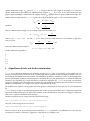
The JOSTLE executable user guide : Version 3.1
Chris Walshaw
School of Computing & Mathematical Sciences,
University of Greenwich, London, SE10 9LS, UK
email: [email protected]
July 6, 2005
Contents
1
The JOSTLE executable package
2
2
Running jostle
2
2.1
The input graph file . . . . . . . . . . . . . . . . . . . . . . . . . . . . . . . . . . . . . . . . . . . . . . . . . . . . . . . .
2
2.2
The number of subdomains . . . . . . . . . . . . . . . . . . . . . . . . . . . . . . . . . . . . . . . . . . . . . . . . . . . .
3
2.3
The output partition file . . . . . . . . . . . . . . . . . . . . . . . . . . . . . . . . . . . . . . . . . . . . . . . . . . . . . .
3
2.4
Repartitioning . . . . . . . . . . . . . . . . . . . . . . . . . . . . . . . . . . . . . . . . . . . . . . . . . . . . . . . . . . .
4
2.5
Disconnected Graphs . . . . . . . . . . . . . . . . . . . . . . . . . . . . . . . . . . . . . . . . . . . . . . . . . . . . . . .
4
2.5.1
Isolated nodes . . . . . . . . . . . . . . . . . . . . . . . . . . . . . . . . . . . . . . . . . . . . . . . . . . . . . . .
4
2.5.2
Disconnected components . . . . . . . . . . . . . . . . . . . . . . . . . . . . . . . . . . . . . . . . . . . . . . . .
4
3
4
5
6
Customising the behaviour
4
3.1
Balance tolerance . . . . . . . . . . . . . . . . . . . . . . . . . . . . . . . . . . . . . . . . . . . . . . . . . . . . . . . . .
4
3.2
Dynamic (re)partitioning . . . . . . . . . . . . . . . . . . . . . . . . . . . . . . . . . . . . . . . . . . . . . . . . . . . . .
5
Additional functionality
6
4.1
Troubleshooting . . . . . . . . . . . . . . . . . . . . . . . . . . . . . . . . . . . . . . . . . . . . . . . . . . . . . . . . . .
6
4.2
Timing jostle . . . . . . . . . . . . . . . . . . . . . . . . . . . . . . . . . . . . . . . . . . . . . . . . . . . . . . . . . .
6
4.3
Memory considerations . . . . . . . . . . . . . . . . . . . . . . . . . . . . . . . . . . . . . . . . . . . . . . . . . . . . . .
6
4.3.1
6
Memory requirements . . . . . . . . . . . . . . . . . . . . . . . . . . . . . . . . . . . . . . . . . . . . . . . . . .
Advanced/experimental features
7
5.1
Heterogeneous processor networks . . . . . . . . . . . . . . . . . . . . . . . . . . . . . . . . . . . . . . . . . . . . . . .
7
5.2
Variable subdomain weights . . . . . . . . . . . . . . . . . . . . . . . . . . . . . . . . . . . . . . . . . . . . . . . . . . .
7
Algorithmic details and further information
8
1
1 The JOSTLE executable package
The jostle executable package comprises this userguide and one or more executable files compiled for different
machines (e.g. jostle.sgi) as requested on the licence agreement. Copies of the executable are available for most
UNIX based machines with an ANSI C compiler and the authors are usually able to supply others.
The package also includes an example graph, tri10k.graph & tri10k.coords. The file tri10k.coords contains
the x & y coordinates of the graph nodes but is not actually required for partitioning since jostle does not use
geometrical information.
2 Running jostle
jostle (i.e. jostle.sgi, jostle.linux, etc.) is run with two inputs – the graph filename and the required number
of subdomains. These can either be entered on the command line, e.g.
jostle tri10k 32
or at the prompt. jostle will first try to open the file [filename] and if that fails it will try [filename].graph
2.1
The input graph file
1
4
3
2
6
7
5
jostle uses the Chaco file input format, [1] (also used by Metis, [3]). In its simplest form the initial line of the file
should contain the integers N , the number of nodes in the graph, and E, the number of edges. There should then
follow N lines each containing the lists of neighbours for the corresponding node (with the nodes being numbered
from 1 up to N ). An example graph is shown above and the graph file is then
7
2
1
1
6
6
3
2
10
3
3 7
2 6 7
7
4 5 7
3 5 6
In more detail, there are 7 nodes and 10 edges in the graph; node 1 is adjacent to 2 & 3; node 2 is adjacent to 1, 3 & 7;
etc.
The graph may also have weighted nodes and edges and the initial line should then contain a third integer, the format,
to specify which. The possible formats are
format
0
1
10
11
node weights
unitary
unitary
user specified
user specified
edge weights
unitary
user specified
unitary
user specified
2
If node weights are required they should be specified as an integer, one on each of the N lines, prior to the neighbour
lists. If edge weights are required they are specified after each neighbour (i.e. the weight for edge (n1 , n2 ) is specified
after n2 on the line corresponding to n1 ).
To give some examples, suppose that node 3 of the example graph has weight 12 and all the rest have weight 1, then
the graph file would be specified as
7 10
1 2
1 1
12 1
1 6
1 6
1 3
1 2
10
3
3 7
2 6 7
7
4 5 7
3 5 6
Alternatively, suppose that edge (4,6) has weight 9, all the rest have weight 1 and the nodes are unweighted, then the
graph file would be specified as
7
2
1
1
6
6
3
2
10 1
1 3 1
1 3 1
1 2 1
9
1 7 1
1 4 9
1 3 1
7 1
6 1 7 1
5 1 7 1
5 1 6 1
Note that the weight 9 occurs twice; once on the line corresponding to node 4 (the 4th line after the header) after the
entry 6 and once on the line corresponding to node 6 (the 6th line after the header) after the entry 4.
Finally, suppose that all nodes and edges have unit weights, as in the first example, but we wish to explicitly record
this in the file, then the graph file would be specified as
7
1
1
1
1
1
1
1
10 11
2 1 3
1 1 3
1 1 2
6 1
6 1 7
3 1 4
2 1 3
1
1 7 1
1 6 1 7 1
1
1 5 1 7 1
1 5 1 6 1
The graph must be undirected so that if an edge (n1 , n2 ) appears then the corresponding edge (n2 , n1 ) must also appear,
and if the edge weights are user specified, they must both have the same weight. Node and edge weights should be
positive integers although nodes with zero weights are allowed. For example to use graphs with non-contiguous sets
of nodes, the missing nodes can be treated as having zero weight and zero degree (i.e. not adjacent to any others).
Finally the file may be headed by an arbitrary number of comments, (lines beginning with % or #) which are ignored.
2.2
The number of subdomains
. . . should be an integer 2 ≤ P N .
2.3
The output partition file
After partitioning a graph, the partition is written out into a file [filename].ptn, where [filename] is the name
of the original graph input file. This file will contain N lines each containing one integer p, with 0 ≤ p < P , giving the
resulting assignment of the corresponding node.
3
2.4
Repartitioning
To repartition a mesh, call jostle with the -repartition flag set, e.g.
jostle -repartition tri10k 16
The code will then open the corresponding .ptn file (described above) and read the existing partition. Note that the
-repartition flag should come before any customised settings (see below).
2.5
Disconnected Graphs
Disconnected graphs (i.e. graphs that contain two or more components which are not connected by any edge) can
adversely affect the partitioning problem by preventing the free flow of load between subdomains. In principle it is
difficult to see why a disconnected graph would be used to represent a problem since the lack of connections between
two parts of the domain implies that there are no data dependencies between the two parts and hence the problem
could be split into two entirely disjoint problems. However, in practice disconnected graphs seem to occur reasonably
frequently for various reasons and so facilities exist to deal with them in two ways.
2.5.1
Isolated nodes
A special case of a disconnected graph is one in which the disconnectivity arises solely because of one or more isolated
nodes or nodes which are not connected to any other nodes. These are handled automatically by jostle. If desired
they can be left out of the load-balancing by setting their weights to zero, but in either case, if not already partitioned,
they are distributed to all subdomains on a cyclic basis.
2.5.2
Disconnected components
If the disconnectivity arises because of disconnected parts of the domain which are not isolated nodes, then jostle
may detect that the graph is disconnected and abort with an error message or it may succeed in partitioning the graph
but may not achieve a very good load-balance (the variation in behaviour depends on how much graph reduction is
used). To check whether the graph is connected, use the graph checking facility (see §4.1). To partition a graph that is
disconnected use the setting
connect = on
This finds all the components of the graph (ignoring isolated nodes which are dealt with separately) and connects
them together with a chain of edges between nodes of minimal degree in each component. However, the user should
be aware that (a) the process of connecting the graph adds to the partitioning time and (b) the additional edges are
essentially arbitrary and may bear no relation to data dependencies in the mesh. With these in mind, therefore, it
is much better for the user to connect the graph before calling jostle (using knowledge of the underlying mesh
not available to jostle). Finally note that, although ideally these additional edges should be of zero weight, for
complicated technical reasons this has not been implemented yet and so the additional edges have weight 1 (which
may be included in the count of cut edges).
3 Customising the behaviour
jostle has a range of algorithms and modes of operations built in and it is easy to reset the default environment to
tailor the performance to a users particular requirements.
3.1
Balance tolerance
As an example, jostle will try to create perfect load balance while optimising the partitions, but it is usually able to
do a slightly better optimisation if a certain amount of imbalance tolerance is allowed. The balance factor is defined as
4
B = Smax /Sopt where Smax is the weight of the largest subdomain and Sopt is the optimum subdomain size given by
Sopt = dG/P e (where G is the total weight of nodes in the graph and P is the number of subdomains). The current
default tolerance is B = 1.03 (or 3% imbalance). To reset this, to 1.05 say, run
jostle imbalance=5 tri10k 16
or
jostle "imbalance = 5" tri10k 16
Note that if there is whitespace in the setting then the quotation marks are required (so that jostle interprets it
as a single argument). Alternatively, create a file called defaults in the same directory as the jostle executable
containing the line
imbalance = 5
The command line settings have a higher priority than the defaults file. Thus if jostle is called with a command
line setting, the defaults file is ignored.
Note that for various technical reasons jostle will not guarantee to give a partition which falls within this balance
tolerance (particularly if the original graph has weighted nodes in which case it may be impossible).
3.2
Dynamic (re)partitioning
Using jostle for dynamic repartitioning, for example on a series of adaptive meshes, can considerably ease the
partitioning problem because it is a reasonable assumption that the initial partitions at each repartition may already
be of a high quality. Recall first of all from §2.4 that to reuse the existing partition the flag -repartition must be
used. One optimisation possibility then is to increase the coarsening/reduction threshold – the level at which graph
coarsening ceases. This should have two main effects; the first is that it should speed up the partitioning and the
second is that since coarsening gives a more global perspective to the partitioning, it should reduce ‘globality’ of the
repartitioning and hence reduce the amount of data that needs to be migrated at each repartition (e.g. see [5]). Currently
the code authors use a threshold of 20 nodes per processor which is set with
threshold = 20
However, this parameter should be tuned to suit particular applications.
A second possibility, which speeds up the coarsening and reduces the amount of data migration is to only allow nodes
to match with local neighbours (rather than those in other subdomains), and this can be set with
matching = local
However, this option should only be used if the existing partition is of reasonably high quality.
For a really fast optimisation, without graph coarsening use
reduction = off
which should also result in a minimum of data migration. However, it may also result in a deterioration of partition
quality, and this will be very dependent on the quality of both the initial partition and also how much the mesh changes
at each remesh. Therefore, for a long series of meshes it may be worth calling jostle with default settings every 10
remeshes or so to return to a high quality partition.
Finally note that some results for different jostle configurations are given in [10]. The configuration JOSTLE-MS is
the default behaviour if jostle is called without an existing partition. The settings to achieve similar behaviour as
the other configurations are
Configuration
JOSTLE-D
JOSTLE-MD
JOSTLE-MS
Setting
reduction = off
threshold = 20, matching = local
–
5
4 Additional functionality
4.1
Troubleshooting
jostle has a facility for checking the input data to establish that the graph is correct and that the graph is connected.
If jostle crashes or hangs, the first test to make, therefore, is to switch it on with the setting
check = on
The checking process takes a fair amount of time however, and once the call to jostle is set up correctly it should be
avoided.
Note that, if after checking, the graph still causes errors it may be necessary to send the input to the authors of jostle
for debugging. In this case, jostle should be called with the setting
write = input
jostle will then generate a subdomain file, jostle.nparts.sdm, containing the input it has been given, and this data
should be passed on to the jostle authors.
4.2
Timing jostle
The code contains its own internal stopwatch which can be used to time the length of a run. It is switched on once the
main routine is called and includes the time for the code to construct its own graph but does not include the time to
read the input nor write the output. The timing routine used is times which gives cpu usage. Note that for optimal
timings the output_level should be set to 0 and the graph checking (§4.1) should not be switched on.
By default the output goes to stderr but this can be changed with the setting
timer = stdout
to switch it to stdout, or
timer = off
to switch it off entirely.
4.3
4.3.1
Memory considerations
Memory requirements
The memory requirements of jostle are difficult to estimate exactly (because of the graph coarsening) but will depend
on N (the total number of graph nodes) and E (the total number of graph edges). In general, if using graph coarsening,
at each coarsening level N is approximately reduced by a factor of 1/2 and E is reduced by a factor of approximately
2/3. Thus the total storage required is approximately 2N + 3E.
The memory requirement for each node is 3 pointers, 3 int’s and 5 short’s and for each edge is 2 pointers and 2 int’s.
On 32-bit architectures (where a pointer and an int requires 4 bytes and a short requires 2 bytes) this gives 36 bytes per
node (strictly it’s 34 but C structures are aligned on 4 byte segments) and 16 bytes per edge. On architectures which
use 64 bit arithmetic, such as the Cray T3E, these requirements are doubled. Thus the storage requirements (in bytes)
for jostle are approximately:
graph coarsening on
graph coarsening off
32-bit
(72N + 48E)
(36N + 16E)
64-bit
(144N + 96E)
(72N + 32E)
6
5 Advanced/experimental features
5.1
Heterogeneous processor networks
jostle can be used to map graphs onto heterogeneous processor networks in two ways (which may also be combined). Firstly, if the processors have different speeds, jostle can give variable vertex weightings to different subdomains by using processor weights – see §5.2 for details.
For heterogeneous communications links (e.g. such as SMP clusters consisting of multiprocessor compute nodes with
very fast intra-node cmmmunications but relatively slow inter-node networks) a weighted complete graph representing the communications network can be passed to jostle. For an arbitrary network of P processors numbered from
0, . . . , P − 1, let lp:q be the relative cost of a communication between processor p and processor q. It is assumed that
these cost are symmetric (i.e. lp:q = lq:p ) and that the cost expresses, in some averaged sense, both the latency and
bandwidth penalties of such a communication. For example, for a cluster of compute nodes lp:q might be set to 1 for
all intra-node communications and 10 for all inter-node communications.
To pass the information into jostle replace the number of subdomains argument by [filename], e.g.
jostle tri10k [filename]
where [filename] is the name of a file containing the upper triangular part of the interprocessor cost matrix. The file
should then be structured as follows
P
l0:1 ,
P (P − 1)/2
l0:2 ,
l1:2 ,
. . . , l0:P −1 ,
. . . , l1:P −1 ,
...,
lP −2:P −1
The first line contains the number of processors P and the number of entries in the upper triangular part of the matrix
(which will be P (P − 1)/2). The following P (P − 1)/2 entries are the upper triangular part of the network cost matrix
(e.g. see [8, Fig. 2]). However since the file is scanned in using the the C scanf() function it does not matter how the
entries are laid out (e.g. one entry per line of the file or all of the entries on one single line of the file will both work).
The choice of the network cost matrix coefficients is not straightforward and is discussed in [8].
5.2
Variable subdomain weights
It is sometimes useful to partition the graph into differently weighted parts and this is done by giving the required
subdomains an additional fixed weight which is taken into account when balancing. For example suppose jostle is
being used to balance a graph of 60 nodes in 3 subdomains. If subdomain 1 were given an additional fixed weight of
10 say and subdomain 2 were given an additional fixed weight of 20, then the total weight is 90 (= 60 + 10 + 20) and
so jostle would attempt to give a weight of 30 to each subdomain and thus 30 nodes to subdomain 0, 20 nodes to
subdomain 1 and 10 nodes to subdomain 2.
These weights can be specified to jostle by running it with the flag -pwt:[filename], e.g.
jostle -pwt:[filename] tri10k 3
where [filename] is the name of a file with P , the number of subdomains, on the first line and then listing the
weights one per line. Thus in the example above file would be
3
0
10
20
Often it is more useful to think about the additional weights as a proportion of the total and in this case a simple
formula can be used. For example, suppose a partition is required where Q of the P subdomains have f times the
7
optimal subdomain weight Sopt (where 0 ≤ f ≤ 1). Suppose that the total weight of the graph is W so that the
optimal subdomain weight without any additional fixed weight is Sopt = W/P . Now let W 0 represent the new total
0
graph weight (including the additional fixed weights) and let Sopt
represent the new optimal subdomain weight. The
0
0
additional fixed weight must be (1 − f ) × Sopt
in each of the Q subdomains and so Sopt
can be calculated from:
0
Sopt
=
0
W + Q(1 − f )Sopt
W0
=
P
P
and hence
0
Sopt
=
W
P − Q(1 − f )
Thus the additional fixed weight on each of the Q subdomains should be set to
0
(1 − f ) × Sopt
= (1 − f ) ×
W
P − Q(1 − f )
Thus if, say, P = 5, Q = 3, W = 900 and f = 1/3 (i.e. three of the five subdomains have one third the weight of the
other two) then
W
900
0
=
= 300
Sopt
=
P − Q(1 − f )
5 − 3(2/3)
and so the additional fixed weight is
0
(1 − f ) × Sopt
= 2/3 × 300 = 200
and the subdomain weight file is
5
0
0
200
200
200
6
Algorithmic details and further information
jostle uses a multilevel refinement and balancing strategy, [6], i.e. a series of increasingly coarser graphs are constructed, an initial partition calculated on the coarsest graph and the partition is then repeatedly extended to the next
coarsest graph and refined and balanced there. The refinement algorithm is a multiway version of the Kernighan-Lin
iterative optimisation algorithm which incorporates a balancing flow, [6]. The balancing flow is calculated either with
a diffusive type algorithm, [2] or with an intuitive asynchronous algorithm, [4]. jostle can be used to dynamically
repartition a changing series of meshes both load-balancing and attempting to minimise the amount of data movement
and hence redistribution costs. Sample recent results can be found in [6, 7, 10].
The modifications required to map graphs onto heterogeneous communications networks (see §5.1) are described in
[8].
jostle also has a range of experimental algorithms and modes of operations built in such as optimising subdomain
aspect ratio (subdomain shape), [9]. Whilst these features are not described here, the authors are happy to collaborate
with users to exploit such additional functionality.
Further information may be obtained from the JOSTLE home page:
http://staffweb.cms.gre.ac.uk/˜c.walshaw/jostle/
and a list of relevant papers may be found at
http://staffweb.cms.gre.ac.uk/˜c.walshaw/papers/
Please let us know about any interesting results obtained by jostle, particularly any published work. Also mail any
comments (favourable or otherwise), suggestions or bug reports to [email protected].
8
References
[1] B. Hendrickson and R. Leland. The Chaco User’s Guide Version 2.0. Tech. Rep. SAND 94-2692, Sandia Natl. Lab.,
Albuquerque, NM, 1994.
[2] Y. F. Hu, R. J. Blake, and D. R. Emerson. An optimal migration algorithm for dynamic load balancing. Concurrency:
Practice & Experience, 10(6):467–483, 1998.
[3] G. Karypis and V. Kumar. Metis unstructured graph partitioning and sparse matrix ordering system version 2.0.
Technical report, Dept. Comp. Sci., Univ. Minnesota, Minneapolis, MN 55455, 1995.
[4] J. Song. A partially asynchronous and iterative algorithm for distributed load balancing. Parallel Comput.,
20(6):853–868, 1994.
[5] C. Walshaw and M. Cross. Load-balancing for parallel adaptive unstructured meshes. In M. Cross et al., editor,
Proc. Numerical Grid Generation in Computational Field Simulations, pages 781–790. ISGG, Mississippi, 1998.
[6] C. Walshaw and M. Cross. Mesh Partitioning: a Multilevel Balancing and Refinement Algorithm. SIAM J. Sci.
Comput., 22(1):63–80, 2000. (originally published as Univ. Greenwich Tech. Rep. 98/IM/35).
[7] C. Walshaw and M. Cross. Parallel Optimisation Algorithms for Multilevel Mesh Partitioning. Parallel Comput.,
26(12):1635–1660, 2000. (originally published as Univ. Greenwich Tech. Rep. 99/IM/44).
[8] C. Walshaw and M. Cross. Multilevel Mesh Partitioning for Heterogeneous Communication Networks. Future
Generation Comput. Syst., 17(5):601–623, 2001. (originally published as Univ. Greenwich Tech. Rep. 00/IM/57).
[9] C. Walshaw, M. Cross, R. Diekmann, and F. Schlimbach. Multilevel Mesh Partitioning for Optimising Domain
Shape. Intl. J. High Performance Comput. Appl., 13(4):334–353, 1999. (originally published as Univ. Greenwich Tech.
Rep. 98/IM/38).
[10] C. Walshaw, M. Cross, and M. G. Everett. Parallel Dynamic Graph Partitioning for Adaptive Unstructured Meshes.
J. Parallel Distrib. Comput., 47(2):102–108, 1997. (originally published as Univ. Greenwich Tech. Rep. 97/IM/20).
9