1
POLCOMS User Guide
V6.4
Jason Holt, March 2008
1.
Introduction................................................................................................................. 3
Background ..................................................................................................................... 3
The scope of POLCOMS ................................................................................................ 3
Using this guide .............................................................................................................. 3
The code.......................................................................................................................... 4
2. Defining the problem .................................................................................................. 4
Control files .................................................................................................................... 5
3. Defining a POLCOMS grid ........................................................................................ 6
Horizontal discretization................................................................................................. 6
case-I boundaries ........................................................................................................ 7
case-II boundaries ....................................................................................................... 9
Open boundaries ......................................................................................................... 9
Vertical discretization ................................................................................................... 10
Initial conditions ........................................................................................................... 11
4. Defining forcing for POLCOMS .............................................................................. 12
Surface forcing.............................................................................................................. 12
ECMWF data ............................................................................................................ 12
Met. Office data ........................................................................................................ 13
Open boundary forcing ................................................................................................. 13
Tidal forcing ............................................................................................................. 14
2
Residual/combined forcing ....................................................................................... 15
Temperature and salinity .......................................................................................... 16
River inputs............................................................................................................... 17
5. Compilation............................................................................................................... 17
Compilation Options..................................................................................................... 19
Compiling Additional Models ...................................................................................... 20
6. Execution .................................................................................................................. 20
Runtime arguments ....................................................................................................... 21
Parallel Execution ......................................................................................................... 22
Running in ensemble mode........................................................................................... 22
7. Output ....................................................................................................................... 23
dailymeanUVT.............................................................................................................. 23
Physseries...................................................................................................................... 24
Appendix A: Model control (CPP directives and logical variables)................................. 25
Appendix B: Principle Model variables............................................................................ 35
Three dimensional arrays.............................................................................................. 35
Two-dimensional arrays at 3 time levels ...................................................................... 37
Two-dimensional arrays................................................................................................ 37
Two-dimensional integer arrays ................................................................................... 39
Appendix C: Model parameters ........................................................................................ 39
Appendix D: Example compiler directive lists................................................................. 40
MRCS – full model....................................................................................................... 40
MRCS – tide only ......................................................................................................... 41
HRCS – Full Model ...................................................................................................... 41
LB – TVD wetting drying............................................................................................. 41
S12 – full model............................................................................................................ 41
Plume ............................................................................................................................ 41
Appendix E: Logical units for input data.......................................................................... 41
Bibliography ..................................................................................................................... 42
POLCOMS_user_guide.doc
3
1. Introduction
Background
The origins of the Proudman Oceanographic Laboratory Coastal Ocean Modelling
System (POLCOMS) lie with studies of frontal dynamics in the North sea for the UK
NERC’s North Sea Project. Since then it has been extensively developed both as a
hydrodynamic and a multi-disciplinary model, including use of its sediment transport
module, coupling to the European Regional Seas Ecosystem model and the Los Alamos
Sea Ice model. Coupling to the GOTM model lends it a range of improved turbulence
models. It has been used extensively in POL and PML’s core research programme, and in
on-going research contracts with the UK Met. Office and a wide range of NERC and EU
funded research project and programmes, notably MERSEA, CASIX, MARPROD,
LOIS, RAPID, ODON. It currently provides the ‘work-horse’ shelf sea model for the UK
marine research centre programme: Oceans 2025, and the National Centre for Ocean
Forecasting.
The scope of POLCOMS
POLCOMS is a three-dimensional baroclinic B-grid model designed for the study of
shelf sea processes and ocean-shelf interaction. Recent work has taken it into estuarine
environments. The model solves the momentum and scalar transport equations for
oceanographic applications with realistic topography, bathymetry and forcing. The
underlying hydrodynamics in POLCOMS are the shallow water equations with the
hydrostatic and Boussinesq approximations. This limits models applicability to flows
where the vertical acceleration is small and in practice this imposes a minimum
horizontal resolution; simulation can be made at resolutions finer than this but at no
benefit to the solution. As a rough guide this can be taken as half the maximum water
depth.
Using this guide
This guide is aimed at providing a new user with a basic introduction to POLCOMS and
to act as a reference for setting up new model domains. It lacks much of the details of the
solution techniques, the most up-to-date reference for this is Holt and James [2001]; a full
technical manual is in preparation.
POLCOMS is a complex model system and a large code (currently standing at around
95,000 lines of code) particularly resulting from the range of options and the parallel
message passing code. To use it effectively requires an understanding of the model
equations and boundary conditions, and how these are represented numerically and
coded. While this document describes many of the options available nothing beats
looking in the code to see what they do.
Throughout this guide the following typographic conventions are used:
POLCOMS_user_guide.doc
4
•
•
•
•
•
Variables in equations in italics e.g. T
Variables names and code in bold e.g. tmp
cpp compiler directives in bold capital e.g. NOSCOORD
Subroutine/module names in bold italics e.g. b3drun
Filenames in bold Arial e.g. b3drun.F
The code
POLCOMS is available under license to collaborators of the Proudman Oceanographic
Laboratory.
The model release ‘un-tars’ into the following directory structure:
pol3db
The source code
v6.3
PMLersemv2.0
CICE
WAM
setups
Additional model codes (available from the
originators)
Application specific subdirectories
plume
MRCS
IRS
The source code consists of:
• *.F
- FORTRAN 90 (fixed format) source with cpp directives:
the main body of code
• *.c
- C source files (used for command line arguments and
GUI)
• *.h
- include files
• makefile
- for compilation control
• objects_*
- lists of source object files for POLCOMS and subsidiary
models
• machine_list
- machine_dependent options
• dependencies_pol3db
- code inter-dependencies
Generally one set of source code is used for all applications, but there is the option of
including application-specific code e.g. for different forms of data output.
The GOTM model should be installed as per instructions on www.gotm.net and is then
used as a library.
2. Defining the problem
Unlike a global model, a regional ocean model is defined for a limited area and as such
can take on a wide range of configurations and domains, each approaching the solution of
the equations in a different fashion and being subject to different forcing. This
requirement for flexibility is controlled in three ways in POLCOMS:
POLCOMS_user_guide.doc
5
•
•
•
cpp compiler directives are used to select portions of the code or exclude others
(e.g. -DNOSCOORD selects σ-coordinates instead of s-coordinates). Many of
these in fact set logical variables in parm_defaults.F. Compiler directives are
most conveniently set in a compilation script specific for the application (e.g.
make_polcoms).
All logical variables defined in the main module (b3d.F) can be set in a name list
file logicalvariables.inp. This overrides the logical variables set by compiler
directives
A number of run-time command-line arguments are available, to set properties
such as length of model run, check-pointing, type of domain decomposition.
Current compiler directives are described in appendix A and options required for several
example applications are listed described in appendix D
Control files
POLCOMS used a number of control files to set basic model parameters and define
input/output files. These can be used in combination with the model described above to
define the model application.
•
parameters.dat defines the grid size, resolution and a number of model
parameters. For the current format see the example in appendix C.
• scoord_params.dat defines parameters for the s-coordinate transform (if
used).
An example is:
150.0d0
hc )
1.0d0
cc ) S coordinate parameters
5.0d0
theta )
0.25d0
bb )
for an explanation of these see Holt and James [2001]
•
•
logicalvariables.inp. A nameslist file setting the logical variables in b3d.F,
see appendix A.
filenames.dat sets the names of input and output files. The format is:
INPUT
input files directory
numnames
input file, 1
.
.
logical unit type
filename
.
.
input file, numnames
OUTPUT
POLCOMS_user_guide.doc
Path to directory of input files
Number of input files
logical unit for filename
6
Number of output file names
Run identifier
numnames
Idname
output file, 1
.
.
logical unit
type
filename
logical unit for filename
.
.
output file, numnames
Data Types are
1. formatted
2. unformatted
3. unformatted, without input directory path
When the model is run it opens all input files in the given path with the given name at the
given unit, and all output files with the suffix “Idname” to identify the run output. Output
files are (by default) written to the directory the model is run in.
Note: the logical units read in here are only used for the purpose of opening the files; they
must match those used in the code. These are usually set in data_out.F for output, see
appendix E for input data units.
3. Defining a POLCOMS grid
As a finite difference model, the spatial discretization on which the equations are solved
is especially important. In POLCOMS this is a B-grid on either spherical polar
coordinates or Cartesian coordinates in the horizontal and terrain following coordinates in
the vertical.
Horizontal discretization
In the horizontal POLCOMS uses a B-grid discretisation, so both components of velocity
(u,v) are defined at u-points, half a grid box to the southwest of points where elevations, ζ
and other scalar variables are defined: b-points (see Figure 1). The domain size is
icg=1..l, jcg=1..m, with (1,1) being the southwest corner. All horizontal arrays have a
halo of at least 1 point (i.e array size is at least (0..l+1,0..m+1)) to facilitate message
passing and open boundary data. Figure 1 shows the arrangement of grid points. The grid
resolution (rdal,rdbe) is set in parameters.dat either as an inverse angular resolution
(in degrees) or in metres for Cartesian coordinates (with directive FLAT). The
coordinates (lat/lon or Cartesian) of the southwest (bottom-left) elevation points (alon0,
alat0 at icg=1,jcg=1) are also set in parameters.dat.
IMPORTANT Because the model is coded for multiprocessor systems almost all the
horizontal indices in the model code (apart from i/o) refer to the LOCAL arrays (i.e.
POLCOMS_user_guide.doc
7
those on a particular processor) and range from i=1,iesub and j=1,jesub. The relation
between LOCAL (i,j) and GLOBAL (icg,jcg) indices is:
icg=i+ielb-1
jcg=j+jelb-1
The model is designed to be highly flexible in its definition of coastal and open
boundaries. Hence there are 7 masks used to define these:
ipexu =1 at u-point where calculations are conducted
ipexb =1 at b-point where calculations are conducted
ipexub =1 at a sea u-point (including coastal points)
ipexbb =1 at a sea b-point
iucoast =1 where u-point is coastal and velocities are evaluated by the lateral
boundary condition (case-II boundaries only, see below)
incb =1 at an open boundary points (always on b-points).
incu =1 at sea u-points next to open boundaries
The distinction between ipexb and ipexbb arises because there can be points across
boundaries that are sea points, but where model calculations are not conducted. Other
more specialized masks (e.g. in the advection routines) are described in the subroutine
documentation.
The bathymetry (hs) is read in at the b-points as an ASCII file by the subroutine hset:
real*8 depth(l,m)
If (leader) then
read(13,*) ((depth(i,j),i=1,l),j=1,m)
endif
call dist (leadid,depth,hs,1)
If the flipbathy logical variable is set then the array is read from north to south rather
than south to north (the defualt).
There are two configurations available as to where the sea-land boundary lies on this
grid.
case-I boundaries
In this case land boundaries lie along b-points (Figure 1) and the primary definition of the
land-sea grid is by the u-points (ipexu) which are either wholly land or sea. In the latter
case each u-point is surrounded by four sea b-points, some of which may be fractional.
This configuration implies a free-slip horizontal boundary condition, which is appropriate
to all but fine resolution simulations. Most calculations occur at the coastal b-points
(ipexb(i,j)=1 here), but the point is surrounded by a fractional grid box (ar(i,j) = 0.5 or
0.25). The grid is defined in boset by reading in ipexu (from an ASCII file in a similar
POLCOMS_user_guide.doc
8
fashion to hs), then by setting ipexb = 1 at all b-points surrounding a u-point where ipexu
= 1. There is a test that the depth hs is non-zero at points with non-zero ipexb.
This configuration allows small islands and peninsulas to be included and gives a subgrid
scale representation of the coastline, but wetting and drying is not available because of
issues of volume conservation that would arise with fractional grid boxes. Model grid
setups should use a procedure such as:
1. Define mask at u-points (ipexu) using the coastline (e.g. use GMT's command
grdlandmask)
2. Calculate mask at b-points (ipexb)
3. Find bathymetry at sea b-points
Matlab (or similar) is useful for this and sometimes iteration from 3 to 1 is needed if the
available bathymetry is not completely consistent with the available coastline.
Figure 1 Case-I boundaries: coastal and open boundary lies along b-points.
A simpler definition of case-I boundaries is available if sub-grid scale coastline
representation is not required. In this case (compiler directive SIMPLECASEI ) only a
bathymetry file is used (no mask file), which defines ipexb; ipexu=1 is then defined
when all four surrounding b-points have ipexb=1.
An alternative method of defining the grid/water depth is provided by the logical options
analytic-depth. In this case FORTRAN files called set_bathymetry.F and
POLCOMS_user_guide.doc
9
set_maks.F are ‘included’. These adjust set the global arrays depth and mask
respectively.
case-II boundaries
In this case land boundaries lie along u-points (Figure 2). Calculations do not occur at the
boundary points, but rather a lateral boundary condition is used, either non-slip (default)
or slip (zero horizontal gradients are imposed with compiler directive UBC). In this
configuration the bathymetry is used to set ipexb (where hs > land), then ipexu = 1 if no
surrounding ipexb = 0. At coastal grid points ipexub = 1 and ipexu = 0. Hence all masks
are derived from the bathymetry (no extra mask file is required) and this significantly
simplifies model setup. This case allows wetting and drying to be implemented but the
need for a horizontal velocity boundary condition is not desirable for coarser resolution
simulations.
Figure 2 Case-II coastal boundaries: coastal points lie alone u-points and open boundary lies along bpoints.
Open boundaries
Open boundaries always lie along b-points (with either case-I or case-II coastal
boundaries), but any point within the domain can be an open boundary point. Open
boundary b-points are indicated by the incb array and the array ifaceob stores which
faces of an open boundary point are open (i.e. receive fluxes from outside the model
domain). By default any point with ipexb(i,j)=1 at icg=1, icg=l, jcg=1, jcg=m is an open
boundary point (this means with case-I boundaries there can not be a coast-line along
these rows/columns, since ipexb = 1 on the coast - the model domain must be extended to
POLCOMS_user_guide.doc
10
accommodate this). In addition to these default points a list of points can be read in of
which faces around any model points are open boundaries (if the directive
READOPENBCPOINTS is set). This reads the ASCII file openbcpoints.dat, which has
the format
npts
icg jcg iface(1)
.
.
.
icg jcg iface(npts)
where npts is the number of additional open faces and the columns list the position of
these (icg,jcg), and which face is open:
iface = 1 south
iface = 2 north
iface = 3 west
iface = 4 east
This allows any shaped open boundary to be defined.
Vertical discretization
The model uses a staggered vertical grid (Figure 3) with state variables defined 1/2 a grid
box above and below the sea surface and bed, and flux variables defined at the surface
and sea bed. Vertical indexing for the state variables is k=2…n-1 (k=1 and k=n are used
for boundary conditions), and for flux variables is k=1..n-1, from the sea bed to the
surface.
The model vertical coordinate is written in -coordinates, but there are two choices of
how the model levels are discretized in -space:
•
•
S-coordinates The level spacing in -space can vary in the horizontal; vertical
coordinate variables ds, dsu, sig, sigo have 3 indices, and separate variables
are defined at u-points: dsv, dsu, sig, sigo.
σ-coordinates The level spacing in -space is fixed in the horizontal.
POLCOMS_user_guide.doc
11
Figure 3 Vertical discretization
Hence in s-coordinates, state variables on b-points (e.g. tmp(k,i,j)) are defined at sig(k1,i,j), are separated by dsu(k-1,i,j) and are associated with a depth, ds(k-1,i,j). Note: the
difference in indexing of -1 from state variables is a historical anomaly which will be
corrected in a future version.
Initial conditions
POLCOMS simulations generally start from rest with a level sea surface (u=v=ζ=0),
currently there are no provisions to initialise the model currents elevations except with a
re-start files. The scalar fields on the other hand, are either initialised to a constant value
(the default), read in from a file or specified from an ‘included’ piece of FORTRAN
code.
With no options the initial T and S are set to the values given in parameters.dat. With
directive READ_INITIAL_TS set they are read from unit 16 according to the format
specified by ts_form in parameters.dat. If ts_form=’unf’ they are read from an
unformatted file otherwise as an ASCII formatted file. Either way they are read as global
3D arrays, temperature then salinity:
real*8 temp3d(l,m,n)
read(16) temp3d
or
real*8 temp3d(l,m,n)
real(16,ts_form) temp3d
POLCOMS_user_guide.doc
12
Alternatively if the ANALYTIC_INIT directive is set a FORTRAN file called
tmpfield.F is ‘included’. This should set the values of tmp and sal at all local b-points.
This is useful for defining idealised problems/test cases.
4. Defining forcing for POLCOMS
In all but the most idealised cases external forcing provides an important control on a
coastal-ocean simulation. POLCOMS includes a wide range of provisions for surface
(metrological), open-boundary (lateral) and riverine/land forcing.
Surface forcing
Complete POLCOMS simulations require surface fluxes of heat (hfl_in, hfl_out),
momentum (fs,gs) and freshwater (ep), and also surface pressure, pr. Apart from
pressure, which is used directly, these are usually defined via bulk formulae from
atmospheric data; the alternative approach, to use fluxes directly from an NWP model
(e.g. the Met. Office applications of POLCOMS), is not described here. The model then
requires the following variables as local arrays (note units):
at
we,wn
rh
cl
pr
pn
air temperature (degrees C)
wind speed, eastwards and northwards (m/s)
relative humidity (%)
cloud cover (%)
atmospheric pressure (mb)
precipitation (ms-1)
The data are read in in metset.F, which is currently ‘hard-wired’ to a number of fixed
data types. The data is read in on the native grid and frequency of the atmospheric model
data set (e.g. as provided by BADC), a copy is passed to each processor and is then
interpolated in spaced onto the model grid (this is efficient for coarse resolution
atmospheric data, but could be improved with parallel input for large data sets). Note: no
distinction between u-points and b-points is made in the interpolation, both use b-point
value with the same index. Input infrequency is set by the istress, icloud, isalt variables
defined in parameters.dat.
The model includes code for reading met. data on the Northwest European shelf from two
sources. Work in the GCOMS project will generalise this to any region around the globe.
ECMWF data
This is the default and refers to either reanalysis (ERA40) or operational products. Data is
read from 3 files: From unit 17, we, wn, pr, at, rh; from unit 21. cl; from unit 89, pn.
Optionally solar radiation (sr) is read from unit 87. In each case the data is on a grid of
size nx x ny = 41x26 staring at -25E, 40N and read from an ASCII file:
read(17,’(10f8.2)’) ((modata1(j,k), j=1,nx), k=1,ny)y.
POLCOMS_user_guide.doc
13
In a number of cases the daily accumulation files (cloud cover, precipitation and solarradiation) are provided in a ‘north to south’ format. The directives FLIPCLD and
FLIP_PRCP accommodate this. This data are converted from day-1 to s-1
Met. Office data
There are two sources here, differing in resolution: the mesoscale model (~12km;
directive MESOMET) and a sub-set of the global model data (1o; directive GLOBMET
). In each case data is provided as one file per variable. Logical units are:
at
20
pr
17
rh
19
we
18
wn
24
cl
21
ep
15
Note in this case rh is specific humidity rather than relative humidity; this is accounted
for in heatin.F by the directive SHUMID.
The mesoscale data uses unformatted files and has nx x ny = 218x136 starting at -13E,
48.39N and a resolution of 0.11. The global data sub-set uses formatted files and has nx x
ny = 42x47 starting at -20.4166E, 39.7233N and a resolution of 0.833 lon and 0.5555 lat.
Open boundary forcing
Open boundary forcing consists of elevations and barotropic currents (tidal and residual
or combined), and temperature and salinity. A depth varying component of current can
also be included in an advective scalar boundary condition. Apart from the radiation
component of the barotropic forcing, these are all ‘active’ boundary conditions in that
they require the specification of external values for the variables. This is appropriate for
nesting in tidally active flows, but more work on the passive boundary conditions (e.g.
implementing an Orlanski condition) is required.
When a model domain is run three files are produced which list the required location of
open boundary conditions. These are
openbclist_z
openbclist_u
openbclist_b
elevation points on the boundary
velocity points outside the boundary
elevation points outside the boundary
Each has the format
nzbc
ipt jpt
.
.
.
Number of points, nzbc, nzbc,nbbc
Global index of each open boundary point
POLCOMS_user_guide.doc
14
ipt jpt(npts)
This then defines the data (and order of the data) required in the open boundary forcing
files. The files can be produced by executing the model, but without running any time
steps: <exename> -tdur 0, and then used to generate boundary condition data for the first
model run.
Tidal forcing
Barotropic tidal elevation and currents are forced using a flux/radiation scheme (with
READ_TIDECON). Tidal velocities are used to calculate a volume flux into/out of each
boundary elevation point, which is used in the standard model equations in barot. The
elevation at these grid points is also relaxed towards the imposed tidal elevation at a rate
proportional to the long wave phase speed √gh (a ‘Flather radiation condition’).
Tidal data is provided to the model either according to the lists described above or across
the whole of the four boundaries of a rectangular model domain. Information about the
tidal constituents to be used is defined in a tidal definition file (unit 43). This has the
format:
ncond number of constituents
nfac flag >0 to use date information
idate <hours day month year> corresponding to the start of the model run or
series of runs (start_time), usually t=0s.
indx which of a standard list of 15 each of 1..ncond tidal constituents refers to.
1) Q1, 2) O1, 3) P1, 4) S1, 5) K1, 6) 2N2, 7) MU2, 8) N2, 9) NU2, 10) M2, 11)
L2, 12) T2, 13) S2, 14) K2, 15 M4.
mcon =1 or =0 depending on whether each of the ncond constituents is to be used
This information is used to apply nodal factors and date corrects to give the correct tidal
phase for the specified date. The assumption being the data is provided in dateindependent form (if this is not the case set nfac=0). The format for the tidal data
depends on the whether the LONGBCFORM is used. The file (unit 14) starts with the
tidal frequencies:
sigma(1)
.
.
.
sigma(ncond)
frequency of 1st constituent in degrees/hour
frequency of ncondth constituent in degrees/hour
then the default is to read:
do i=1,ncond
read(itide,'(8f10.6)') (z1(j,i),j=1,nzbc)
read(itide,'(8f10.6)') (z2(j,i),j=1,nzbc)
POLCOMS_user_guide.doc
15
read(itide,'(8f10.6)') (u1(j,i),j=1,nubc)
read(itide,'(8f10.6)') (u2(j,i),j=1,nubc)
read(itide,'(8f10.6)') (v1(j,i),j=1,nubc)
read(itide,'(8f10.6)') (v2(j,i),j=1,nubc)
enddo
from unit itide=14. z1 and z2 are the cosine and sine components of the elevation of each
constituent (similarly for velocity, u and v)
If LONGBCFORM is used data is read according to
do i=1,ncond
read(itide,'(8f10.6)') (z1(j,i),j=1,nobdZ)
read(itide,'(8f10.6)') (z2(j,i),j=1,nobdZ)
read(itide,'(8f10.6)') (u1(j,i),j=1,nobdUV)
read(itide,'(8f10.6)') (u2(j,i),j=1,nobdUV)
read(itide,'(8f10.6)') (v1(j,i),j=1,nobdUV)
read(itide,'(8f10.6)') (v2(j,i),j=1,nobdUV)
enddo
where nobdZ=2l+2m, nobdUV=(2(l+1)+2(m+1) and the data is ordered east to west and
north to south along the southern, northern, eastern then western boundaries (irrespective
of whether points are land or sea).
The boundary tidal currents are then calculated from these constituents at each barotropic
time step. If directive ZBAR is used the equilibrium tide is also used.
Residual/combined forcing
As well as tidal forcing time series of barotropic elevation and current can be applied
around the model boundaries. These either represent the residual, in which case they are
additive with the tidal component, or they can be used to provide the full forcing. The
Data are read from unit nrm=77 at a format (default is *, boundzuv_form=’unf’ for
unformatted) and frequency (in hours) set in parameters.dat (less than 1 hour
currently causes an error). At each time data is read in using
read(nrm,*) (z1(j),j=1,nzbc)
read(nrm,*) (u1(j),j=1,nubc)
read(nrm,*) (v1(j),j=1,nubc)
and similarly for the unformatted case. z1, u1, v1 are boundary currents and elevations.
These are ramped linearly in time between concurrent values and applied as boundary
conditions as described above. A LONGBCFORM is also available in a similar format
to the tidal constituents.
If only elevations are available these can be imposed using a relaxation condition (set
using (READ_ZET; this has not been extensively tested).
POLCOMS_user_guide.doc
16
Temperature and salinity
Two options are provided for scalar boundary conditions, an up-wind advective scheme
and a relaxation scheme. Currently the list data format is only available for the advective
scheme – the relaxation scheme is limited to the longer format and hence only rectangular
domains. The type of T and S boundary condition data is controlled by the file
boundarycon.h:
c #define TS_boundary_condition bost
c #define TS_boundary_condition boundaryTS
#define TS_boundary_condition boundaryTS_longform
c#define TS_boundary_condition bfix
c#define TS_boundary_condition no_bc
The appropriate sub-routine is un-commented.
For advective boundary conditions data is provided one grid cell outside the model
domain and the boundary condition currents used to advect it into the domain on inflow.
Data frequency is set in parameters.dat and at each time data is read from unit
nrmt=78 by:
do j=1,nbbc
read(nrmt,*) Iin,Jin,(btmp1(k,j),k=1,n-2)
enddo
do j=1,nbbc
read(nrmt,*) Iin,Jin,(bsal1(k,j),k=1,n-2)
enddo
unless bounts_form=’unf’ in which case
do j=1,nbbc
read(nrmt) (btmp1(k,j),k=1,n-2)
enddo
do j=1,nbbc
read(nrmt) (bsal1(k,j),k=1,n-2)
enddo
is used. Data is ramped linearly in time at each time step.
For relaxation conditions the width of the relaxation zone (niw) is set in
parameters.dat. The relaxation coefficient is set to vary linearly from 1 (clapped) at
the open boundary to zero at niw+1 points in side the model. Data is read uses
read(nrmt,*) ((btmp1(k,j),k=1,n-2),j=1,nobw)
read(nrmt,*) ((bsal1(k,j),k=1,n-2),j=1,nobw)
POLCOMS_user_guide.doc
17
where nobw=2l+2m unless VARY_RELAX is set. In this case the imposed data can
vary across the relaxation zone and nobw=2.niw.l+2.niw.m. Data is ordered east to west
and north to south along the southern, northern, eastern then western boundaries
(irrespective of whether points are land or sea). If VARY_RELAX is set this is repeated
for kk =1 to niw points inside the model domain using the provided data, otherwise the
data at the boundary is used across the relaxation zone (note: side length does not
decrease as kk increases).
A number of FORTRAN program are available to extract boundary condition data from
POLCOMS output for use as forcing for a smaller (and usually finer resolution) domain.
River inputs
A simple approach for applying river forcing is used: this is to increase the sea surface
elevation according to the volume flux, with a corresponding adjustment to the salinity
through the water column. The river locations are provided by an index file (unit 29) that
lists the model grid points. The file starts with nofriv (number of rivers in the domain)
then the locations are given in a range of formats:
Default (36 NW shelf rivers):
read(29,'(i2,1x,a14,2(1x,i3))') idriv(nr),name,icriv(nr),jcriv(nr)
If NORIVTMP is set (40 years NW shelf database of ~300 rivers):
read(29,'(i3,2(i4),1x,a20)') idriv(nr),icriv(nr), jcriv(nr),name
If CEH set (40 year data base of UK rivers)
read(29,'(i3,1x,a19,2(1x,i3))') idriv(nr),name,icriv(nr),jcriv(nr)
The format for the river data is one row per day and one column per river. The number of
rivers in the database (i.e. number of columns) is set in parameters.dat, and which of
these is in the domain is given by the array idriv.
5. Compilation
Compilation is carried out using an application specific script (make_polcoms) from
the application directory (e.g. pol3db/setups/plume). For example:
#!/bin/csh -f
set OPTS = ("-DFLAT -DNOTIDE -DRIVERS -DNO_SCOORD -DADV_BC")
set OPTS = ($OPTS " -DNOCOMPRESS -DANALYTICINIT DANALYTIC_DEPTH -DANALYTIC_INIT -DRIVERFIX")
set MACHINE = shelf-ibmcluster
POLCOMS_user_guide.doc
18
set POLDIR = ../../v6.3
set MAKEDIR = $cwd
set EXE_NAME = shelf
#copy application specific files
cp boundarycon.h
$POLDIR
cp data_out.F
$POLDIR
cp tmpfield.F
$POLDIR
cp set_bathymetry.F $POLDIR
cp set_mask.F
$POLDIR
#enter source directory
cd $POLDIR
#compile
#make clean
make $MACHINE "OPTIONS= $OPTS " “MAKE_TARGET=polcoms”
cd $MAKEDIR
#return to application directory and copy in executable.
cp $POLDIR/$EXE_NAME ./
exit(0)
In this example the OPTS variable sets a list of complier directives (see appendix A) to
define the model problem, use MACHINE to choose one of the computer dependent
‘make targets’ in machine_list, and the MAKE_TARGET variable choose which
selection of models is to be compiled. The makefile currently includes the following
options:
•
•
•
•
•
polcoms
polcoms_gotm
polcoms_gotm_ersem
polcoms_ersem
polcoms_wam
Each also requires the corresponding cpp directives to be set: -DERSEM, -DGOTM,
-DWAM.
The optional make clean statement will remove all object files and .f files so compilation
will start from scratch (usually not necessary).
Compilation proceeds in two stages:
Each FORTRAN source file (.F) is compiled in turn by make: first compiler directives
are resolved to give a .f file then these are compiled with the FORTRAN compiler e.g.
POLCOMS_user_guide.doc
19
cpp –D….. b3drun.F b3drun.f
f90 –r8
-c
The resulting .f files should not be edited
b3drun.F -o b3drun.o
Then all object files (.o) files are linked to create the executable. The default executable
name is shelf.).
Compilation Options
The make targets in machine_list provide the compilation options required for each
different computer/compiler. They are also used for different compilation and linking
options e.g. for debugging and profiling and to set paths to libraries. Three examples are
shown.
A linux workstation with debugging on:
shelf-linux-pg-g:
$(MAKE) $(MAKE_TARGET) "OPTIONS=$(OPTIONS)" \
"OPTIONS=$(OPTIONS)" "DEBUG=$(DEBUG)" \
"PROGRAM=$(PROGRAM)" \
"SIZE=$(SIZE)" "ENV=SERIAL" \
"CPP=cpp" \
"CPPFLAGS=-P -traditional" "CPPMACH=-DLINUX" \
"CC=pgf90" "CFLAGS=-Ktrap=fp -g" \
"FC=pgf90" "FFLAGS= -g -r8 -Ktrap=fp -Mprof -Mextend " \
"OFLAGS=" "GFLAGS=" "PFLAGS=" \
"LOPTS= -L /packages/netcdf/netcdf-3.5.1/lib -lnetcdf" \
"LIBS=$(LIBS)"
The POL IBM cluster, using MPI:
shelf-ibmcluster-mpi:
$(MAKE) $(MAKE_TARGET) "OPTIONS=$(OPTIONS)" \
"OPTIONS=$(OPTIONS)" "DEBUG=$(DEBUG)" \
"EXE=$(EXE)" \
"SIZE=$(SIZE)" "ENV=MPI" \
"CPP=/lib/cpp" \
"CPPFLAGS=-P -traditional" "CPPMACH=-DLINUX \
-I/usr/local/mpichgm/include/" \
"CC=mpicc" "CFLAGS= -Ktrap=fp -D_FILE_OFFSET_BITS=64 " \
"FC=mpif90" "FFLAGS= -r8 -O2 -Mlfs -Ktrap=fp –Mprof
-byteswapio " \
"OFLAGS=" "GFLAGS=" "PFLAGS=" \
"LOPTS= -Mprof" \
POLCOMS_user_guide.doc
20
"LIBS=$(LIBS)"
The HPCx, IBM Power 5:
shelf-regatta-mpi:
$(PMAKE) $(MAKE_TARGET) \
"OBJECTS=$(OBJECTS)" "DEPENDS=$(DEPENDS)" \
"NPES=$(NPES)" \
"OPTIONS=$(OPTIONS)" "DEBUG=$(DEBUG)" \
"PROGRAM=$(PROGRAM)" \
"ENV=MPI" \
"CPP=/lib/cpp" "CPPFLAGS=-P" "CPPMACH=
I/usr/lpp/ppe.poe/include/thread64 -DIBM" \
"CC=cc" "CFLAGS=-q64" \
"FC=mpxlf90_r" "OFLAGS=-O2 -qarch=pwr4 -qtune=pwr4 -qhot qsuppress=1500-036" \
"GFLAGS=" "PFLAGS=" "FFLAGS=-q64" \
"F77FLAGS=-qfixed" "F90FLAGS=-qsuffix=f=f90" \
"LFLAGS=-L/usr/local/lib" \
"LIBS=$(LIBS)"
For each new computer POLCOMS is compiled/run on a new target is required in
machine_list, following this template.
Compiling Additional Models
POLCOMS has been coupled to a range of different modelling systems; notably, ERSEM
(ecosystem model), GOTM (turbulence model), CICE (sea ice model) and WAM (wave
model). Generally the additional model code is placed in a subdirectory of the
POLCOMS source code directory. An objects list file is provided in the POLCOMS
directory and ‘included’ by the makefile. The POLCOMS makefile is then used for the
additional model (including the machine_list options) and all object files created are
linked to produce the executable. If there are connections between modules then these
need to specified in the makefile with a –I option. Note: the dependencies of additional
models are not explicitly specified. This means, for example, if a POLCOMS module that
the ERSEM model uses is changed, “make clean” should be used for both POLCOMS
and ERSEM codes, and the compilation started from scratch. An exception to this
procedure is GOTM, which is installed as a library and then linked in.
6. Execution
The mode of execution depends on particular computer used, its job submission system
and whether the code is run in batch or interactive mode. Apart from the simplest single
processor execution on a stand alone workstation, a batch processing script is required to
request resources and control the multi-processor execution.
POLCOMS_user_guide.doc
21
Runtime arguments
The follow command line options are available (except when the NOGUI directive is
used):
Model command line options:
-help
: Print this usage information
-quiet
: Suppress stdout monitor
-verbose
: Adds debugging info to monitor
-tdur
: Run length (hours)
-nstep
: Run length (timesteps)
-mnth
: Month number for input
-particles
: Enable particle tracking
-indir
: Directory for input data files
-flipcld
: flips cloud data from north-south to south-north
Restart/checkpointing:
-warm_start : Start from restart file
-restart
: Start from restart file
-reset
: Resets time, u, v, zet
-restm
: Resets time on restart to start_time
-tchk
: Checkpoint interval (hours)
-nchk
: Checkpoint interval (timesteps)
-tcmin
: Time of first checkpoint (hours)
-ncmin
: Timestep of first checkpoint (hours)
-tfwnd
:Forward-wind input data (hours)
Parallel processing:
-nproc
: Number of processes (not usually required)
-nprocs
: Number of processes
````
-nprocx
: Number of processes in x
-nprocy
: Number of processes in y
-nens
: Number of ensemble members
-asynch
: Use asynchronous comms
-immed
: Use non-blocking comms
-promis
: Use promiscuous receives
-nocomms
: Disable boundary exchange
-noimmed
: Use blocking comms
-nosndrcv
: Do not use send/receive mode
-simple
: Use simple partitioning
-sndrcv
: Use send/receive mode
-synch
: Use synchronous comms
-partrk
: Use RK partitioning
-map
: Print partitioning map to file
Client/Server operation:
-server
: Start POLCOMS as server
POLCOMS_user_guide.doc
22
Debugging:
-idbg
-jdbg
-kdbg
: Debugging point x-coordinate
: Debugging point y-coordinate
: Debugging point z-coordinate
An important feature available from these run-time options is check-pointing/restarting.
For example:
cp filenames.jan01 filenames.dat
./shelf –tdur 744. –tchk 744.
cp filenames.feb01 filenames.dat
./shelf –tdur 672. –tchk 672. -restart
will run shelf for two legs (January 2001 and February 2001), check pointing at the end
of the first then restarting at the start of the second. This allows a long simulation to be
broken down into manageable sections e.g. to fit in the constraints of a batch queuing
system.
Parallel Execution
In a normal parallel execution environment in which the number of processors is
specified as part of the batch job script or interactive options, POLCOMS picks up the
number of processors automatically from the size of the MPI_Comm_World
communicator. If necessary the number of processors can be set using the –nprocs
command line option. By default, POLCOMS automatically partitions the grid in the two
horizontal dimensions using a recursive partitioning algorithm. This balances the number
of sea points across the processors in order to obtain the optimum run-time load balance.
Usually the default settings are those which will work best and give the best performance.
The number of processors is factored in two dimensions as near square as possible e.g. on
8 processors then nprocx=4 and nprocy=2. If a different factorization is required this can
be specified using the –nprocx and –nprocy options. The –simple option disables the
recursive partitioning in favour of a scheme which divides the domain without any regard
to the distribution of sea points. The –map option may be used to write a map of the
portioned domain to a file in PPM format. The netpbm package
(http://netpbm.sourceforge.net/) may be used to convert this file to an image e.g. using
the ppmtogif command. Options –asynch and –synch switch between asynchronous and
synchronous communications i.e. normal MPI sends and synchronous MPI sends.
Options –immed and –noimmed switch between normal MPI sends and immediate MPI
sends. The option –nocomms may be used to disable all nearest neighbour boundary
exchange. Whereas this invalidates the results of the code it is useful to compare timings
with and without communications.
Running in ensemble mode
It is possible to run POLCOMS in ensemble mode where a number of independent model
runs are combined in a single job. To enable this specify the command line option –nens
e.g –nens 16. For example when running on 64 processors this will execute 16
POLCOMS_user_guide.doc
23
independent model runs with 4 processors each (except see later). In order to specify
different parameters for each ensemble member POLCOMS looks for individual copies
of the files parameters.dat and filenames.dat of the form parameters_001.dat,
parameters_002.dat etc. and filenames_001.dat and filenames_002.dat etc. If
these files are not found then each ensemble member runs with the same standard
parameters.dat and filenames.dat files. In this way every aspect of the forcing,
initial data and output files for the ensemble members may be customized. If different
bathymetry files are specified for each ensemble member then POLCOMS reads these
first before assigning processors and the number of processors per ensemble member is
balanced according to the number of sea points. The standard output from each ensemble
member is reassigned to a file named output_001, output_002 etc.
7. Output
POLCOMS has a range of output options controlled by the subroutine data_out. This is
an application specific code that is copied into the source directory at compile time, it
calls generic output routines contained in out.F and tidemeanout.F. The general
procedure for spatial arrays is to copy data to the leader processor (using standard
communications routines) and output from here. For output at a specific grid cell, a test is
required that that cell is on a particular processor: if ( ielb.le.icg .and. icg.le.ieub .and.
jelb.le.jcg .and. jcg.le.jeub ) then. ... The logical units set by filenames.dat need to be
consistent with those used in data_out.F. Typically a model run uses unformatted
compressed binary output for high-volume data (e.g. 3D fields) and formatted output for
others. Two examples are described here;
dailymeanUVT
These files are used to output 25 hour means of tmp, sal, u, and v, and also spm if used.
It can use a compressed format to only output at sea points. In which case, a header is
written first containing the size of the grid and the location of the sea b-points. This is
repeated for u-points. Then the 3D model fields are output daily. FORTRAN code to read
these files is like:
real*4, allocatable, dimension (:,:,:) :: tmp,sal,u,v
integer, allocatable, dimension (:) :: isea,jsea,iusea,jusea
.
.
read(1) l,m,n,npsea
if ( .not. allocated(isea)) allocate(isea(npsea),jsea(npsea))
read(1) isea
read(1) jsea
read(1) l,m,n,npusea
if ( .not. allocated(iusea)) allocate(iusea(npusea),jusea(npusea))
read(1) iusea
read(1) jusea
POLCOMS_user_guide.doc
24
if ( .not. allocated(tmp) ) then
allocate(tmp(l,m,n-2))
allocate(sal(l,m,n-2))
allocate(u(l,m,n-2))
allocate(v(l,m,n-2))
endif
do it=1,ntimes
read(1) itimt
read(1) ((u(iusea(i),jusea(i),k),k=1,n-2),i=1,npusea)
read(1) ((v(iusea(i),jusea(i),k),k=1,n-2),i=1,npusea)
read(1) ((tmp(isea(i),jsea(i),k),k=1,n-2),i=1,npsea)
read(1) ((sal(isea(i),jsea(i),k),k=1,n-2),i=1,npsea)
Note: the binary format of the input and output system must match. As most systems now
use IEEE floating point format this is not usually a problem, though there can be an issue
with file record structures and big-endian versus little-endian. POLCOMS is generally set
up to use UNIX (rather than PC/LINUX) style binaries.
Physseries
This outputs data at a list of grid points typically every hour. The files are opened
with,e.g. call initseries(200,'physseries'). This will read from unit 88 a list of ioutpt
points and for each of this open a file physseries.<i>.RUNID to unit 200+i. each call to
outseries (e.g. call outseries_wcol(200,ioutpt)) writes depth profiles of u,v, tmp, aa, ak,
qsq, al and spm if used. Variables are converted to integer unless REALSERIES is
defined. MATLAB code to read these files is like
load physseries…
ni=8
np=length(physseries)/ni;
i=1:np;
t=i/24;
k=2:n-1
ii=ni-1
eval(['clear aa' RunID '_' Id ])
eval(['clear ak' RunID '_' Id ])
eval(['clear qsq' RunID '_' Id ])
eval(['clear al' RunID '_' Id ])
eval(['time' RunID '_' Id '=physseries(ni*i-ii,1);']);
eval(['u' RunID '_' Id '=physseries(ni*i-ii,k)/1000;ii=ii-1;']);
eval(['v' RunID '_' Id '=physseries(ni*i-ii,k)/1000;ii=ii-1']);
eval(['tmp' RunID '_' Id '=physseries(ni*i-ii,k)/1000;ii=ii-1']);
eval(['sal' RunID '_' Id '=physseries(ni*i-ii,k)/1000;ii=ii-1']);
eval(['aa' RunID '_' Id '(:,2:n-1)=physseries(ni*i-ii,k)/100000;ii=ii-1']);
eval(['ak' RunID '_' Id '(:,2:n-1)=physseries(ni*i-ii,k)/100000;ii=ii-1']);
eval(['qsq' RunID '_' Id '(:,2:n-1)=physseries(ni*i-ii,k)/100000;;ii=ii-1']);
POLCOMS_user_guide.doc
25
eval(['al' RunID '_' Id '(:,2:n-1)=physseries(ni*i-ii,k)/1000;;ii=ii-1']);
Work is in progress to replace these files with NetCDF
(http://www.unidata.ucar.edu/software/netcdf/).
Appendix A: Model control (CPP directives and logical
variables)
Unless otherwise specified the default value of logical variables is .false.
Compiler directive
METOFFICE
Logical variable
GULF
AMM
IRSH
MRCS
advection
advect_v
ADV_BC
adv_bc
ANALYTIC_DEPTH
analytic_depth
ANALYTIC_INIT
analytic_init
ATTEN
BALTIC
BIHARM
POLCOMS_user_guide.doc
Baltic
Description
Needed if using met.
office heat fluxes and
system
A Met. Office domain
A Met. Office domain
A Met. Office domain
A Met. Office domain
Do momentum and scalar
advection
Advect v component of
momentum
Used advective boundary
conditions (otherwise
relaxation)
Set bathymetry to
idealised values defined
in set_bathymetry.F
Set an analytic buoyancy
(temperature) field,
defined in tmpfield.F
Use IOP derived
attenuation coefficients
for heating and ecosystem
model
Include the Baltic as an
inflow
Biharmonic, rather than
Laplacian in sigmacoordinate horizontal
diffusivity (NOT
TESTED)
26
BIO_LAMDA
bio_lambda
BNDUADV
BULKMET
bulk_met
BULK_COARE
BULK_NSP
CEH
CICE
ceh
cice
CLOUDPOINT
cloudpoint
COARSEGRID
COASTFRIC
COEF_NSP
COLLECTIVE
COMPOUT
compress
CONST_TS_BC
CONST_HORIZ_DIF
POLCOMS_user_guide.doc
const_ts_bc
Use transmissivity from
the ERSEM model in the
heatflux calculation
Include boundary points
in velocity advection –
acts as ‘Sommerfeld’ type
passive boundary
condition
Read met data from
files(s) (pressure, winds,
temperature, relative
humidity and cloud cover)
Use COARE 3 bulk heat
flux
Use Goldsmith and
Bunker Heat bulk heat
flux
Use CEH UK river data
Use the Los Alamos
CICE sea ice model
a single value of cloud
data is read to represent
the cloud over the whole
domain at each time; use
with BULKMET
Setup a coarse resolution
grid to run alongside
standard model
Increase z0 near coast not stable
Interpolate latitude
dependent heat flux
parameters
Use collective
communication routines
Only output tide means at
sea points
Use compressibility term
in equation of state for
HPG.
Boundary temperature
and salinity values are
held constant (values read
in from file)
Constant diffusivity in σcoordinate horizontal
27
CONVECTU
convect_u
CTDTRACK
DEBUG
plus extra debugging
information on:
DEBUG_MODEL
DEBUG_ADV
DEBUG_B3DRUN
DEBUG_BAROC
DEBUG_BAROT
DEBUG_CONVECT
DEBUG_DIFFUSEB
DEBUG_DIFFUSEU
DEBUG_HORIZUV
DEBUG_HORIZTS
DEBUG_PGRAD
DEBUG_LAGRANGE
DEBUG_EXCHANGE
DEBUG_COMMS
DEBUG_GLOBCOM
DEBUG_LAGRANGE
DEBUG_STRSET
physics model
advection
main program control
baroclinic integration
barotropic integration
convective adjustment
scalar diffusion
velocity diffusion
Horizontal diff. u,v.
Horizontal diff T & S.
Pressure gradient
Particle tracking
Halo exchange
Communications
Global communications
Partical tracking
Met. Data input
DIA_F
dia_f
DIA_T
dia_t
DSSRDATA
DSTRDATA
POLCOMS_user_guide.doc
diffusivity, otherwise,
Smagorinsky
Convective adjustment
for u, v, temperature and
salinity (not advisable)
Output T, S and SPM
profiles according to a list
of time, long. and lats.
Output a range of
information and specific
values of variables at the
debuging point. For use in
debugging.
Output flux data for T and
S budget
Output temperature
diagnostics at specified
points and in 3D
Use downward SW
radiation forcing rather
than astronomical
calculation corrected for
clouds. Requires albedo
Use downward thermal
radiation forcing
28
DOCUMENT
ERSEM
EXTRARIVS
extrarivs
FOAM
FORCEafterDIFF
FLAT
Flat
FLIPBATHY
flipbathy
FLIPCLD
flipcld
FLIP_PRCP
flip_prcp
FLIP_RAD
flip_rad
GLOBMET
globmet
GOTM
HARM_ANA
HARMW
HORIZDIF
Horizdif
HORIZTS
Horizdifts
POLCOMS_user_guide.doc
Make the POLCOMS
documentation
Use ERSEM
Use constant annual mean
data for additional rivers
Fix for missing FOAM
b.c. data
Moving surface forcing to
occur after vertical
diffusion
Use Cartesian coordinates
- daldi and dbedi in
parameters.dat represent
dx and dy in metres.
Bathymetry file is read in
by row from north to
south (default is south to
north)
Cloud data is read in by
row from south to north
(default is north to south)
Precipitation data is read
in by row from south to
north (default is north to
south)
SW radiation data is read
in by row from south to
north (default is north to
south)
Use Met. Office’s Global
NWP data
Use the General Ocean
Turbulence Model to
calculate vertical
diffusivities
Do harmonic analysis and
output harmonic constants
to file
Include the vertical
velocity in the harmonic
analysis calculations
(requires HARM_ANA
too)
Add horizontal diffusion
to currents - on Z -levels
Do horizontal diffusion of
29
HORIZ_DIF_SIG
HORIZ_DIF_SIG_TS
hor_press_grad
IBM
INVERSE_B
inverse_b
IRREG_BC
irreg_bc
key_EnKF
Key_EnOI
key_ENSEMBLEOUT
key_clderr
temperature and salinity
(requires HORIZDIF too)
Add horizontal diffusion
to currents - on σ-levels
Do horizontal diffusion of
temperature and salinity
(requires
HORIZ_DIF_SIG too)
Switch on/off hpg
Machine dependent
option for IBM systems
(e.g. HPCx)
Apply inverse barometer
correction at the boundary
- used when boundary
data elevations do not
include the effects of
atmospheric pressure but
either BULKMET or
POINTMET is used
Use irregular shaped
relaxation zone T&S
b.c.’s
Use ensemble Kalman
Filter assimilation
Use ensemble optimal
interpolation assimilation
Perturb cloud cover in
ensemble Kalman filter
key_ImpSam
key_turberr
key_winderr
key_1DASSIM
lchkpnt
lfwnd
lnoout
looping
LOCOMS
LONGBCFORM
POLCOMS_user_guide.doc
longbcform
Do full checkpoint at time
intervals tchk
Forward-wind forcing
data by time tfwnd
Suppress output
Run Low resolution
Coastal-Ocean Model, in
addition to POLCOMS
use long format boundary
conditions - south, north,
west, east
30
lwarm
MPI
MONITOR
MESOMET
mesomet
MY25CBF
my25cbf
NOCOMPRESS
OLD_UR_VR
NO_CONVADJ
ncep_lcd
NODIFF
nodiff
NOHPG
NOCLI
NOMODEL
NO_PGRAD
NOPHYSADV
NO_RAMP
NORIVERSKIP
POLCOMS_user_guide.doc
riverskip
Read in full restart data
Use MPI for message
passing
Output largest current
speed
Use Met. Office’s
mesoscale NWP data
Set a spatially varying
coefficient of bottom
friction (otherwise
constant)
Omit the pressure term
from the calculation of
'potential buoyancy'.
Required if not using scoordinates.
Use original calculation
of depth varying
component of volume
fluxes in scalar advection
Do not do a convective
adjustment (default with
GOTM on)
Use cloud data from
NCEP (to replace
ERA40)
Switch off vertical
diffusion
Switch off horizontal
pressure gradient
calculation
Make b3drun.F the main
program, needed for error
trapping with Portland
Compilers but disables
command line arguments
Omit the physics model
calculations
Calculate the horizontal
pressure gradientalong σlevels
Turn off all physics
advection
Do not ramp up the initial
wind forcing
Read in river data from
31
NORIVTMP
NOROT
norot
NO_SAL
no_sal
NOSCAADV
NO_SCOORD
no_tmp
scoord
NOSPMADV
NOSPMRIV
NOSPMSOURCE
lspmsource
NOSLIP
NOSTEEP
NOSTEEPZ
NOTEVENSIG
NOTIDE
no_tide
NO_TMP
NO_V
NOVELADV
ONESPMADV
OUTSCOORD
outscoord
PARALLEL_STATS
part_tracking
PGRAD
POLCOMS_user_guide.doc
lpgrad
start of file instead of
skipping nday-1 records
Do not read in river
temperatures
No rotation - Coriolis
force is zero
Turn off salinity
integration
Turn off scalar advection
Use σ- rather than scoordinates
Turn off advection of
SPM
Turn off spm input from
rivers
Turn off coastal sources
of SPM
Turn off steepening
during calculation of
horizontal advection
Turn off steepening
during calculation of
vertical advection
σ-levels are not evenly
spaced (redundant)
Run without tide or
residual forcing
Turn off temperature
integration
Turn off northwards
advection
Turn off velocity
advection
Only advect the first SPM
class
Output 3d array of scoordinates; run will stop
as soon as file is written
Output parallel statistics
Use particle tracking submodel
Calculate the horizontal
pressure gradient by
interpolating onto
32
PGRAD_SPLINE
lpgrad_spline
PGRAD_TEST
pgrad_test
physmodel
POINTMET
point_met
POLARSTEREO
PROGDENS
progdens
PVM
Q2L
q2l
RAMPTIDE
READ_INITIAL_TS
read_initial_ts
READOPENBCPOINTS
readopenbcpoints
READ_TIDECON
read_tidecon
READ_ZETUB
read_zetub
READ_ZET
read_zet
REALSERIES
reset
POLCOMS_user_guide.doc
horizontal plane (default
linear interpolation)
Default = .true.
Calculate the horizontal
pressure by spline
interpolation onto
horizontal plane
Execute the physics
model
Use single point met data:
pressure, winds,
temperature, relative
humidity and cloud cover
Use polarstereo project
for horizontal coordinates
Set buoyancy =
temperature i.e.
equivalent to linear
equation of state
Use PVM for message
passing (not recently
tested)
Use lengthscale equation
in MY turbulence closure
(not tested)
Increase tidal constituents
from zero at start of run
Read initial temperature
and salinity fields from
file
Read additional open
boundary locations from
file
Read tidal constituents
from file.
Read from file boundary
elevations and currents at
frequency set in
parameters.dat
Read boundary elevations
from file for ‘elevation
only’ boundary condition
Use floating point format
for time seriesoutput
Time and currents reset to
33
resetweekmeans
RILIMIT
rilimit
RIMIX
rimix
RIVERFIX
RIVERS
rivers
resettm
SALFLUX
salflux
SALTFLUX
lsaltflux
SCOORD_EVEN
scoord_even
SCOORD
SCINTERP
SERIAL
Server
SHMEM
SPM
POLCOMS_user_guide.doc
lspm
zero – allows spin up of T
and S.
Weekly means are
initialized at the start of
this run
Option on limiting the
mixing length in
turbulence routines
Use the Richardson
number dependent
boundary layer mixing
scheme
Elevation is modified by
river inflow at a river grid
box during baroclinic
(rather than barotropic
time step
Include freshwater inflow
from rivers
Reset time to be
start_time, rather than
time from resart file
Include salinity flux
calculations
Read in surface
precipitation data
s-levels are equallyspaced in the vertical
(same as -levels),
irrespective of the water
depth
Use horizontally varying
vertical coordinate
(default: .true.)
Use original calculation
of s-coordinates at upoints
Run on single processor
machine
Run POLCOMS as a
server.
Use Cray SHMEM library
for message passing in
addition to MPI/PVM
(not recently tested)
Use the SPM submodel
34
SSRDATA
spm_advection
ssrdata
Stdout
TIMING
Timing
TIMING_ADV
TIMING_BAROC
TIMING_BAROT
TSFLUX
TVD
TRACER
Tracer
UBC
UBC__CALC
UCOAST
ucoast
UNFORMMET
unformmet
VAMPIR
VARY_LAMBDA
vary_lambda
VARY_REALAX
vary_realax
POLCOMS_user_guide.doc
Advect SPM
Use net SW radiation
forcing rather than
astronomical calculation
corrected for clouds
Write monitor output to
stdout on this processor
Output timing
information for various
stages of the model run
Include detailed timing
for advection routines
Include detailed timing
for baroclinic integration
Include detailed timing
for barotropic integration
Output horizontal T and S
fluxes
Use TVD wetting and
drying (with WETDRY)
Advection and diffusion
of a passive tracer
Use non-zero tangential
velocities at coastal
boundaries (for use with
case II boundaries)
Calculate velocities at
coastal-points (with
UCOAST). Not fully
tested
Use case II boundaries land boundaries lie along
u-points (default is case I)
Use unformatted
meteorological data files
(specific implementation)
Use vampire profiler
Use a water depth
dependent transmissivity
in the SW downwelling
calculation
Use a relaxation boundary
condition for temperature
and salinity with forcing
values changing across
the relaxation zone
35
Use code optimized for
vector machine (i.e. not
cache optimized)
Write time steps to screen
Add wave coupling terms
Use WAM wave model
Use wetting/drying code
Add a fluctuation
component (read in from
file) to the wind field
Include the equilibrium
tide in barotropic
calculation
In the pressure gradient
calculation use zero
pressure gradient near bed
boundary condition
(default is zero density
gradient)
use depth-varying
currents in T and S
advective boundary
condition
VECTOR
Verbose
Waves
WAVES
WAM
WETDRY
WINDFLUC
Wetdry
Windfluc
ZBAR
Lzbar
ZERO_PG_BC
zero_pg_bc
ZVARYBC
Zvarybc
Appendix B: Principle Model variables
Variables defined in module b3d.F
Three dimensional arrays
•
real*8, dimension(n,1-mhalo:iesub+mhalo,1-mhalo:jesub+mhalo)
Variable
aa
ah
Description
Vert. viscosity
Horiz viscosity
Units
m2s-1
m2s-1
ak
aka
Vert. diffusivity
Viscosity for slow
baroclinic step
Temporary array
Mixing length
Buoyancy
Boundary sal.
Boundary tmp
Volume flux (u)
m2s-1
m2s-1
File changed in
turbulence.F
horizdiffusivity.F,
horizdiffuse.F
turbulence.F
b3drun.F
m2s-1
m
ms-2
p.s.u.
o
C
m2s-1
b3drun.F
turbulence.F
bcalc.F
boundaryTS.F
boundaryTS.F
barot.F
ak_temp
al
b
bsal
btmp
fu
POLCOMS_user_guide.doc
36
fv
fus
fvs
qsq
sal
Volume flux (v)
Volume flux (u) for
slow baroclinic step
Volume flux (v) for
slow baroclinic step
T.K.E.
Salinity
m2s-1
m2s-1
barot.F
b3drun.F
m2s-1
b3drun.F
m2s-2
p.s.u.
turbulence.F
advect_sca.F, saltflux.F,
diffuse.F
advect_sca.F, downwell.F,
diffuse.F
advdif_spm.F
o
tra
Potential
temperature
Tracer
u
Eastward velocity
ms-1
v
Northward velocity
ms-1
uo
u velocity at last
time step
v velocity at last
time step
Depth varying
velocity (u)
Depth varying
velocity (v)
Vertical velocity
Mixing length
profile
Level
Level width
Level spacing to
surface and sea bed
Level width at upoints
Level spacing at upoints
s-levels for state
variables, b-point
s-levels for state
variable, u-point
s-level for flux
variable, b-point
s-level for flux
variable, u-point
25 hours means, aa
25 hours means, ak
ms-1
baroc.F, barot.F diffuse.F,
advect_vel.F
baroc.F, barot.F, diffuse.F,
advect_vel.F
turbulence.F
ms-1
turbulence.F
ms-1
baroc.F
ms-1
baroc.F
ms-1
-
Turbulence.F
-
sigmaset.F, scoordset.F
sigmaset.F, scoordset.F
sigmaset.F, scoordset.F
-
scoordset.F
-
scoordset.F
-
sigmaset.F, scoordset.F
-
scoordset.F
-
sigmaset.F, scoordset.F
-
scoordset.F
m2s-1
m2s-1
tidemeanout.F
tidemeanout.F
tmp
vo
ur
vr
w
aln
ds
dsu
dsup
dsv
dsuv
sig
sigv
sigo
sigov
aastor
akstor
POLCOMS_user_guide.doc
C
m-3
37
ustor
vstor
al_stor
spmstor1
spmstor2
tuflx
tvflx
suflx
25 hours means, sal
25 hours means,
tmp
25 hours means, u
25 hours means, v
25 hours means, al
25 hour mean, spm1
25 hour mean, spm2
tmp flux u
tmp flux v
sal flux u
svflx
sal flux b
rowbar
pressure
Mean density
Pressure for
compressibility calc.
Worker arrays for
advection routines
..
..
..
..
salstor
tmpstor
d_bl
d_br
d_dba
d_dmb
d_db
d_d2b
d_fuu
d_fba
sigo2
Aku
epsilon
p.s.u.
o
C
tidemeanout.F
tidemeanout.F
ms-1
ms-1
m
gm-3
gm-3
o
C m2s-1
o
C m2s-1
p.s.u.
m2s-1
p.s.u.
m2s-1
kgm-3
Pa
tidemeanout.F
tidemeanout.F
tidemeanout.F
tidemeanout.F
tidemeanout.F
tidemeanout.F
tidemeanout.F
tidemeanout.F
-
advpb[uv].F
..
..
..
diffusivity at u-point m2s-1
Dissipation
m2s-3
tidemeanout.F
bcalc.F
bcalc.F , pgrad.F, p
advpb[uv].F
advpb[uv].F
advpb[uv].F
advpb[uv].F
advpb[uv].F
advpb[uv].F
advpb[uv].F
advpb[uv].F
turbulence.F
turbulence.F
Two-dimensional arrays at 3 time levels
•
real*8, dimension(1-mhalo:iesub+mhalo,1-mhalo:jesub+mhalo,3)
Variable
Zet
Ub
Vb
Description
Elevation
Depth mean current
u
Depth mean current
v
Units
m
ms-1
File changed in
barot.F
barot.F
ms-1
barot.F
Two-dimensional arrays
•
real*8, dimension(1-mhalo:iesub+mhalo,1-mhalo:jesub+mhalo)
Variable
Description
POLCOMS_user_guide.doc
Units
File changed in
38
Afnlb
Ar
At
Bfnlb
cdb
Cl
Csq
Dzdt
Ep
Fb
Fs
Flxu
Flxv
Gb
Gs
H
h1
h2
h22
hfl_in
hfl_out
Hs
Hsu
Hu
hu1
hu2
hu22
Pn
Pr
Sr
Rh
Relfac
Depth mean of nonms-2
linear/buoyancy
terms u
Fraction area of grid
cell
o
Air temperature
C
Depth mean of nonms-2
linear/buoyancy
terms u
Bottom friction
coefficient
Cloud cover
%
‘old’ bottom friction
ms-1
term
elevation changes
ms-1
Precipitation minus
ms-1
evaporation
Bottom stress u
m2s-2
Surface stress u
m2s-2
Volume flux u
m2s-1
Volume flux v
m2s-1
Bottom stress v
m2s-2
Surface Stress v
m2s-2
Total water depth
m
Intermediate water
m
depth
..
m
..
m
o
Heat flux in
Cms-1
o
Heat flux out
Cms-1
Undisturbed water
m
depth
Undisturbed water
m
depth u-points
Water depth u-points m
Intermediate water
m
depth
..
m
..
m
Precipitation
ms-1
Atmospheric pressure mb
Shortwave Rad.
Wm-2
Relative humidity
%
Relaxation zone
factor
POLCOMS_user_guide.doc
baroc.F
b3dgrid.F
metset.F
baroc.F
cbfset.F
metset.F
barot.F
out.F
Saltflux.F
barot.F
metset.F
tidemeanout.F
tidemeanout..F
barot.F
metset.F
barot.F
Advect_sca.F
Advect_sca.F
Advect_sca.F
heatin.F
heatin.F
hset.F
b3dgrid.F
barot.F
Advect_vel.F
Advect_vel.F
Advect_vel.F
metset.F
metset.F
metset.F
metset.F
bost.F
39
Eastward wind
Northward wind
Equilibrium tide
Elevation boundary
condition
Accumulated change
in elevation
Limit for equation in
very shallow water.
We
Wn
Zbar
Zetbc
Dzb
Dlim
ms-1
ms-1
m
m
m
metset.F
metset.F
tidbndrp2.F
tidbndrp2.F,
boundaryUVZ.F, bcbr.F
barot.F
-
barot_tvd.F
Two-dimensional integer arrays
•
integer, dimension(n,1-mhalo:iesub+mhalo,1-mhalo:jesub+mhalo)
Variable
Iapbu
Iapbv
Iapuu
Iapuv
Incb
Incu
Ipexb
Ipexu
ipexbb
ipexub
irel
iucoast
Description
Advection mask
..
..
..
point is at open
boundary
u-point is next to
open boundary
Calculation mask- b
calculation mask- u
land-sea mask – b
land sea mask – u
relaxation zone –
points from
boundary
coastal u-point
File changed in
advset.F
advset.F
advset.F
advset.F
setopenbc.F
setopenbc.F
boset.F
boset.F
boset.F
boset.F
relzone.F
b3dgrid.F
Appendix C: Model parameters
This is an example parameters.dat file from the MRCS domain:
251
l )
206
m )
20
n )
10.0d0
hsmin
'(53f6.2)'
bathf
'(50i2)'
maskf
'(20f8.4)'
ts_form
'(41(1x,f3.0))'
'50f8.4' bounts_form
POLCOMS_user_guide.doc
Model grid dimensions
Minimum water depth
Format for bathymetry
Format for mask data
Format for initial temperature & salinity
format for cloud data
boundary T S format (only use for =unf)
40
'20f8.4' bounzuv_form boundary U,V,zeta format (only use f
10.0d0
daldi
Inverse longitude resolution (degrees)
15.0d0
dbedi
Inverse latitude resolution (degrees)
-11.9875d0
along1
Western limit of domain B-point (1,1)
48.00833d0
alat1
Southern limit of domain B-point (1,
0.0d0
st
Start time
20.0d0
dlt
Barotropic time step
15
mt
Time step ratio
4
mts
Number of fast baroclinic steps
744.0
tdur
Run Length
1.0d-5
avmin
Minimum Diffusivity
1.0d-15
dbdzmin Minimum buoyancy gradient in TKE equations.
1.0d-6
q2min
Minimum turbulent energy
200.0d0
ahm
Coefficent for Killworth Filter
0.2
ahc
Coefficient for Smag. or constant h.diff
1.0
prt
Turbulent Prandlt number
0.005d0
cbf
Constant or min. coeff. of bottom friction
3.0d-3
z0
Bottom roughness length
10000.0d0
conv_lim Maximum depth for convective adjustment
0.0d0
land
value for dry land in bathymetry data
6.0d0
rstress )
24.0d0
rcloud ) Frequency of forcing (hours)
24.0d0
rsalt )
6
ntypes
Number of met. data variables
24.0d0
bounfreq_TS Frequency of T and S boundary data (hours)
1.0d0 bounfreq_ZET Frequency of U,V,ZET boundary data (hours)
171
ig )
184
jg )
Debugging co-ordinates
2
kg )
8.0d0
tmp_init
Initial temperature
35.1d0
sal_init
Initial salinity
38
noriv
Number of rivers in data base
0.01
ddry wetting-drying - depth at which points are 'dry'
0.5
zwet change in elevation to next grid point forwetting
1
niw
Numer of points in relaxation zone.
Appendix D: Example compiler directive lists
MRCS – full model
SPM, MY25CBF, READOPENBCPOINTS, RIVERFIX, BULKMET, INVERSE_B
RIVERS, TIMING, READ_TIDECON, READ_INITIAL_TS, BALTIC, ADV_BC,
CLOUDPOINT, NOSTEEP, ONESPMADV, BNDUADV, SCINTERP,
REALSERIES, NOCOMPRESS, PGRAD_SPLINE,VARY_LAMBDA,
COMPOUT, CTDTRACK
POLCOMS_user_guide.doc
41
MRCS – tide only
MY25CBF, READOPENBCPOINTS, NO_TMP, NO_SAL, TIMING,
READ_TIDECON, NOSTEEP, BNDUADV, SCINTERP, NOCOMPRESS,
NOHPG, COMPOUT, HARM_ANA
HRCS – Full Model
COMPOUT, MY25CBF, BULKMET, NOSTEEP, UCOAST, BALTIC, BNDUADV,
VARY_LAMBDA, READOPENBCPOINTS, FLIPCLD, HORIZ_DIF_SIG,
HORIZ_DIF_SIG_TS, ADV_BC, NOCOMPRESS, RIVERS, READ_ZETUB
TIMING, RIVERS, RIVERFIX, READ_INITIAL_TS, NORIVTMP, ZVARYBC,
TRACER, TRACERSTART, BNDUADV, DIA_F, SCINTERP
LB – TVD wetting drying
READ_TIDECON, NO_SCOORD, FLIPBATHY, MY25CBF, NOCOMPRESS,
UCOAST, WETDRY, TVD, RIVERS, NO_TMP, NO_PGRAD
S12 – full model
MY25CBF, RIVERFIX, BULKMET, INVERSE_B, RIVERS, READ_TIDECON,
READ_INITIAL_TS, BALTIC, NOSTEEP, SALTFLUX, SALFLUX,
PGRAD_SPLINE, NOTMPRIV, COMPOUT, TIMING, FLIPCLD, FLIP_PRCP,
ZBAR, HORIZTS, HORIZDIF, READ_ZETUB, VARY_REALAX, FLIPBATHY,
LONGBCFORM, FOAM, BNDUADV
Plume
BNDUADV, RIVERS, ANALYTIC_INIT, ANALYTIC_DEPTH, FLAT,
NO_SCOORD, NOCOMPRESS
Appendix E: Logical units for input data
Unit
13
12
55
16
17
21
89
87
20
17
19
18
24
15
File description
Mean water depth
ipexu mask
Extra open boundary points
T and S initial conditions
Met. variables for ECMWF forcing
Cloud data
Precipitation data
Shortwave radiation
air temp
Pressure
Humidity
Eastward wind
Northward wind
Precipitation
POLCOMS_user_guide.doc
Subroutine
hset
boset
openbcpoints.dat
bset
interp_met1
interp_met1
interp_met1
interp_met1
interp_meso
interp_meso
interp_meso
interp_meso
interp_meso
interp_meso
42
43
14
77
78
29
30
31
32
117
88
Tidal constituents and start time
Tidal constituent data
Elevation and current boundary data
T and S boundary data
Rivedr index
River flow data
River water temperature
Baltic inflow data
River SPM load
Time series output points
tideset
tideset
boundaryUVZ
boundaryTS
fwin
fwin
fwin
fwin
fwin
filope
Bibliography
Allen, J. I., J. Blackford, J. T. Holt, R. Proctor, M. Ashworth, and J. Siddorn (2001), A
highly spatially resolved ecosystem model for the North West European continental shelf,
SARSIA, 86, 423-440.
Ashworth, M., J. T. Holt, and R. Proctor (2004), Optimization of the POLCOMS
Hydrodynamic Code for Terascale High-Performance Computers, in Proceedings of the
18th International Parallel & Distributed Processing Symposium, 26th-30th April 2004,
edited, Santa Fe, New Mexico.
Ashworth, M., R. Proctor, J. T. Holt, J. I. Allen, and J. C. Blackford (2001), Coupled
Marine Ecosystem Modelling on High Performance Computers, in Developments in
Teracomputing, edited by W. Z. a. N. Kreitz, pp. 150-163.
Cooper, W., C. Hinton, N. Ashton, A. Saulter, C. Morgan, R. Proctor, C. Bell, J. Holt, E.
Young, and Q. Huggett (2006), UK Marine Renewable Energy Atlas, ICE Journal of
Maritime Engineering, In Press.
Holt, J. T., J. I. Allen, R. Procter, and F. Gilbert (2005), Error quantification of a high
resolution coupled hydrodynamic-ecosystem coastal-ocean model: part 1 model overview
and assessment of the hydrodynamics Journal of Marine Systems, 57, 167-188.
Holt, J. T., and I. D. James (1999), A simulation of the Southern North Sea in comparison
with measurements from the North Sea Project. Part 1: Temperature, Continental Shelf
Research, 19, 1087-1112.
Holt, J. T., and I. D. James (1999b), A simulation of the Southern North Sea in
comparison with measurements from the North Sea Project. Part 2: Suspended Particulate
Matter, Continental Shelf Research, 19, 1617-1642.
POLCOMS_user_guide.doc
43
Holt, J. T., and I. D. James (2001), An s-coordinate density evolving model of the North
West European Continental Shelf. Part 1 Model description and density structure,
Journal of Geophysical Research, 106(C7), 14015-14034.
Holt, J. T., and I. D. James (2006), An assessment of the fine scale-eddies in a high
resolution model of the shelf seas west of Great Britain, Ocean Modelling, 13, 271-291.
Holt, J. T., I. D. James, and J. E. Jones (2001), An s-coordinate density evolving model of
the North West European Continental Shelf. Part 2 Seasonal currents and tides, Journal
of Geophysical Research, 106(C7), 14035-14053.
Holt, J. T., and R. Proctor (2003), The role of advection in determining the temperature
structure of the Irish Sea, Journal of Physical Oceanography, 33, 2288-2306.
Holt, J. T., R. Proctor, J. C. Blackford, J. I. Allen, and M. Ashworth (2004), Advective
controls on primary production in the stratified western Irish Sea: an eddy-resolving
model study, Journal of Geophysical Research, 109, doi: 10.1029/2003JC001951.
Lewis, K., J. I. Allen, A. Richardson, J, and J. T. Holt (2006), Error quantification of a
high resolution coupled hydrodynamic-ecosystem coastal-ocean model: part3, Validation
with Continuous Plankton Recorder data, Journal of Marine Systems, 63, 209-224.
Proctor, R., J. T. Holt, J. I. Allen, and J. C. Blackford (2003), Nutrient fluxes and budgets
for the North West European Shelf from a three-dimensional model, Science of the Total
Environment, 313-316, 769-785.
Proctor, R., J. T. Holt, T. R. Anderson, B. A. Kelly-Gerreyn, J. Blackford, and F. Gilbert
(2002), Towards 3-D ecosystem modelling of the Irish Sea., paper presented at Estuarine
and Coastal Modeling Proceedings of the 7th International Conference. American Society
of Civil Engineers, 5-7 November 2001, St. Petersburg Florida.
Siddorn, J. R., J. I. Allen, J. C. Blackford, F. J. Gilbert, J. T. Holt, M. W. Holt, J. P.
Osborne, R. Procter, and D. K. Mills (2007), Modelling the hydrodynamics and
ecosystem of the North-West European continental shelf for operational oceanography,
Journal of Marine Systems, 65, 417-429.
Young, E. F., and J. T. Holt (2007), Prediction and analysis of long-term variability of
temperature and salinity in the Irish Sea, Journal of Geophysical Research, 112,
doi:10.1029/2005JC003386, 002007.
POLCOMS_user_guide.doc
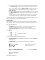
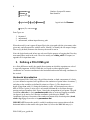


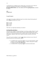
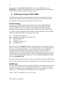
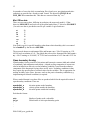

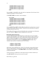

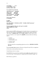
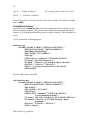
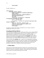

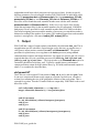
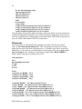

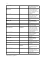
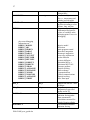
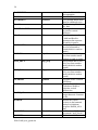
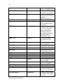
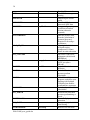
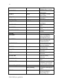
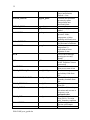
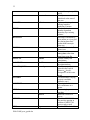
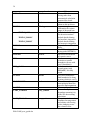
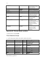
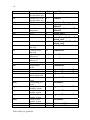
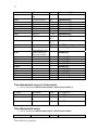
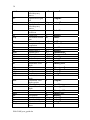
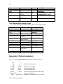

![取扱説明書 [HW-01D] -かんたん操作ガイド-](http://vs1.manualzilla.com/store/data/006640180_2-0d9585ab80892b64753c2bf1419745ad-150x150.png)