Download (TOMS) Data Products User's Guide

NASA
Technical
Publication
1998-206895
Earth Probe Total Ozone
Mapping Spectrometer (TOMS)
Data Products User's Guide
Richard D. McPeters, P. K. Bhartia,
Arlin J. Krueger, and Jay R. Herman
Goddard Space Flight Center
Greenbelt, Maryland
Charles G. Wellemeyer, Colin J. Seftor,
Glen Jaross, Omar Torres, Leslie Moy,
Gordon Labow, William Byerly, Steven L. Taylor,
Tom Swissler, Richard P. Cebula
Raytheon STX Corporation (RSTX)
4400 Forbes Boulevard
Lanham, Maryland
National Aeronautics and
Space Administration
Goddard Space Flight Center
Greenbelt, Maryland 20771
1998
ACKNOWLEDGMENTS
The Level–2 and Level–3 data products described in this User's Guide were prepared by the Ozone Processing Team
(OPT) of NASA/Goddard Space Flight Center. Please acknowledge the Ozone Processing Team as the source of these
data whenever reporting on results obtained using the TOMS data.
The TOMS algorithm development, evaluation of instrument performance, ground-truth validation, and data
production were carried out by the Ozone Processing Team (OPT) at NASA/GSFC. The OPT is managed by the
Nimbus Project Scientist, R. D. McPeters. The current OPT members include Z. Ahmad, G. Batluck, E. Beach, P.
Bhartia, W. Byerly, R. Cebula, E. Celarier, S. Chandra, M. DeLand, D. Flittner, L. Flynn, J. Gleason, J. Herman, E.
Hilsenrath, S. Hollandsworth, C. Hsu, R. Hudson, G. Jaross, N. Krotkov, A. Krueger, G. Labow, D. Larko, J. Miller,
L. Moy, R. Nagatani, P. Newman, H. Park, W. Planet, D. Richardson, C. Seftor, T. Swissler, R. Stolarski, S. Taylor, O.
Torres, C. Wellemeyer, R. Wooldridge, and J. Ziemke.
The TOMS instrument was built and launched by Orbital Sciences Corporation of Pomona, California.
ii
TABLE OF CONTENTS
Section
Page
1.0
INTRODUCTION . . . . . . . . . . . . . . . . . . . . . . . . . . . . . . . . . . . . . . . . . . . . . . . . . . . . . . . . . . . . . . . . . . . . . . . . 1
2.0
OVERVIEW. . . . . . . . . . . . . . . . . . . . . . . . . . . . . . . . . . . . . . . . . . . . . . . . . . . . . . . . . . . . . . . . . . . . . . . . . . . . . 3
2.1
2.2
2.3
2.4
2.5
3.0
INSTRUMENT . . . . . . . . . . . . . . . . . . . . . . . . . . . . . . . . . . . . . . . . . . . . . . . . . . . . . . . . . . . . . . . . . . . . . . . . . . 6
3.1
3.2
3.3
3.4
3.5
3.6
4.0
Accuracy and Precision of TOMS Measurements . . . . . . . . . . . . . . . . . . . . . . . . . . . . . . . . . . . . . . . . . . 24
Calculated Radiances and Their Use in the Algorithm . . . . . . . . . . . . . . . . . . . . . . . . . . . . . . . . . . . . . . 25
Comparison with Fairbanks Ozone Sondes . . . . . . . . . . . . . . . . . . . . . . . . . . . . . . . . . . . . . . . . . . . . . . . 26
Comparison with ADEOS/TOMS . . . . . . . . . . . . . . . . . . . . . . . . . . . . . . . . . . . . . . . . . . . . . . . . . . . . . . 26
Comparison with Ground-based Measurements . . . . . . . . . . . . . . . . . . . . . . . . . . . . . . . . . . . . . . . . . . . 26
PROBLEMS LOCALIZED IN SPACE AND TIME . . . . . . . . . . . . . . . . . . . . . . . . . . . . . . . . . . . . . . . . . . . . . 30
6.1
6.2
6.3
6.4
6.5
6.6
7.0
Theoretical Foundation . . . . . . . . . . . . . . . . . . . . . . . . . . . . . . . . . . . . . . . . . . . . . . . . . . . . . . . . . . . . . . 13
Calculation of Radiances . . . . . . . . . . . . . . . . . . . . . . . . . . . . . . . . . . . . . . . . . . . . . . . . . . . . . . . . . . . . . 15
Surface Reflection . . . . . . . . . . . . . . . . . . . . . . . . . . . . . . . . . . . . . . . . . . . . . . . . . . . . . . . . . . . . . . . . . . 17
Initial B-Pair Estimate . . . . . . . . . . . . . . . . . . . . . . . . . . . . . . . . . . . . . . . . . . . . . . . . . . . . . . . . . . . . . . . 18
Best Ozone . . . . . . . . . . . . . . . . . . . . . . . . . . . . . . . . . . . . . . . . . . . . . . . . . . . . . . . . . . . . . . . . . . . . . . . . 18
Validity Checks . . . . . . . . . . . . . . . . . . . . . . . . . . . . . . . . . . . . . . . . . . . . . . . . . . . . . . . . . . . . . . . . . . . . 21
Level 3 Gridding Algorithm. . . . . . . . . . . . . . . . . . . . . . . . . . . . . . . . . . . . . . . . . . . . . . . . . . . . . . . . . . . 23
GENERAL UNCERTAINTIES . . . . . . . . . . . . . . . . . . . . . . . . . . . . . . . . . . . . . . . . . . . . . . . . . . . . . . . . . . . . . 24
5.1
5.2
5.3
5.4
5.5
6.0
Description. . . . . . . . . . . . . . . . . . . . . . . . . . . . . . . . . . . . . . . . . . . . . . . . . . . . . . . . . . . . . . . . . . . . . . . . . 6
Radiometric Calibration. . . . . . . . . . . . . . . . . . . . . . . . . . . . . . . . . . . . . . . . . . . . . . . . . . . . . . . . . . . . . . . 7
3.2.1 Prelaunch Calibration. . . . . . . . . . . . . . . . . . . . . . . . . . . . . . . . . . . . . . . . . . . . . . . . . . . . . . . . . . . 8
3.2.2 Radiance-Based Calibration Adjustments . . . . . . . . . . . . . . . . . . . . . . . . . . . . . . . . . . . . . . . . . . . 9
3.2.3 Time-Dependent Calibration . . . . . . . . . . . . . . . . . . . . . . . . . . . . . . . . . . . . . . . . . . . . . . . . . . . . . 9
Wavelength Monitoring . . . . . . . . . . . . . . . . . . . . . . . . . . . . . . . . . . . . . . . . . . . . . . . . . . . . . . . . . . . . . . 11
Gain Monitoring. . . . . . . . . . . . . . . . . . . . . . . . . . . . . . . . . . . . . . . . . . . . . . . . . . . . . . . . . . . . . . . . . . . . 11
Attitude Determination . . . . . . . . . . . . . . . . . . . . . . . . . . . . . . . . . . . . . . . . . . . . . . . . . . . . . . . . . . . . . . 11
Validation . . . . . . . . . . . . . . . . . . . . . . . . . . . . . . . . . . . . . . . . . . . . . . . . . . . . . . . . . . . . . . . . . . . . . . . . . 12
ALGORITHM . . . . . . . . . . . . . . . . . . . . . . . . . . . . . . . . . . . . . . . . . . . . . . . . . . . . . . . . . . . . . . . . . . . . . . . . . . 13
4.1
4.2
4.3
4.4
4.5
4.6
4.7
5.0
Instrument . . . . . . . . . . . . . . . . . . . . . . . . . . . . . . . . . . . . . . . . . . . . . . . . . . . . . . . . . . . . . . . . . . . . . . . . . 3
Algorithm. . . . . . . . . . . . . . . . . . . . . . . . . . . . . . . . . . . . . . . . . . . . . . . . . . . . . . . . . . . . . . . . . . . . . . . . . . 4
Data Uncertainties . . . . . . . . . . . . . . . . . . . . . . . . . . . . . . . . . . . . . . . . . . . . . . . . . . . . . . . . . . . . . . . . . . . 4
Archived Products . . . . . . . . . . . . . . . . . . . . . . . . . . . . . . . . . . . . . . . . . . . . . . . . . . . . . . . . . . . . . . . . . . . 5
Near Real-Time Products. . . . . . . . . . . . . . . . . . . . . . . . . . . . . . . . . . . . . . . . . . . . . . . . . . . . . . . . . . . . . . 5
Aerosol Contamination . . . . . . . . . . . . . . . . . . . . . . . . . . . . . . . . . . . . . . . . . . . . . . . . . . . . . . . . . . . . . . 30
Scan Angle Dependence . . . . . . . . . . . . . . . . . . . . . . . . . . . . . . . . . . . . . . . . . . . . . . . . . . . . . . . . . . . . . 31
Solar Eclipses. . . . . . . . . . . . . . . . . . . . . . . . . . . . . . . . . . . . . . . . . . . . . . . . . . . . . . . . . . . . . . . . . . . . . . 32
Polar Stratospheric Clouds. . . . . . . . . . . . . . . . . . . . . . . . . . . . . . . . . . . . . . . . . . . . . . . . . . . . . . . . . . . . 32
High Terrain . . . . . . . . . . . . . . . . . . . . . . . . . . . . . . . . . . . . . . . . . . . . . . . . . . . . . . . . . . . . . . . . . . . . . . . 32
Missing Data . . . . . . . . . . . . . . . . . . . . . . . . . . . . . . . . . . . . . . . . . . . . . . . . . . . . . . . . . . . . . . . . . . . . . . 32
DATA FORMATS . . . . . . . . . . . . . . . . . . . . . . . . . . . . . . . . . . . . . . . . . . . . . . . . . . . . . . . . . . . . . . . . . . . . . . . 33
7.1
Hierarchical Data Format. . . . . . . . . . . . . . . . . . . . . . . . . . . . . . . . . . . . . . . . . . . . . . . . . . . . . . . . . . . . . 33
7.1.1 Level–2 Hierarchical Data Format Product . . . . . . . . . . . . . . . . . . . . . . . . . . . . . . . . . . . . . . . . . 33
7.1.2 Level–3 Hierarchical Data Format Product . . . . . . . . . . . . . . . . . . . . . . . . . . . . . . . . . . . . . . . . . 37
iii
TABLE OF CONTENTS (Continued)
Section
7.2
Page
Native Format. . . . . . . . . . . . . . . . . . . . . . . . . . . . . . . . . . . . . . . . . . . . . . . . . . . . . . . . . . . . . . . . . . . . . . 38
7.2.1 TOMS Ozone File (Level–2 Data Product) . . . . . . . . . . . . . . . . . . . . . . . . . . . . . . . . . . . . . . . . . 38
7.2.2 CDTOMS (Level–3 Data Product) . . . . . . . . . . . . . . . . . . . . . . . . . . . . . . . . . . . . . . . . . . . . . . . 43
REFERENCES. . . . . . . . . . . . . . . . . . . . . . . . . . . . . . . . . . . . . . . . . . . . . . . . . . . . . . . . . . . . . . . . . . . . . . . . . . . . . . . 45
RELATED LITERATURE. . . . . . . . . . . . . . . . . . . . . . . . . . . . . . . . . . . . . . . . . . . . . . . . . . . . . . . . . . . . . . . . . . . . . . 47
LIST OF ACRONYMS, INITIALS, AND ABBREVIATIONS . . . . . . . . . . . . . . . . . . . . . . . . . . . . . . . . . . . . . . . . . 51
APPENDIXES
APPENDIX A. STANDARD OZONE AND TEMPERATURE PROFILES . . . . . . . . . . . . . . . . . . . . . . . . . . . . . . . 53
APPENDIX B. SOFTWARE TO READ HDF OZONE DATA . . . . . . . . . . . . . . . . . . . . . . . . . . . . . . . . . . . . . . . . . 55
APPENDIX C. DATA AVAILABILITY . . . . . . . . . . . . . . . . . . . . . . . . . . . . . . . . . . . . . . . . . . . . . . . . . . . . . . . . . . . 57
APPENDIX D. ATTITUDE ANOMALIES. . . . . . . . . . . . . . . . . . . . . . . . . . . . . . . . . . . . . . . . . . . . . . . . . . . . . . . . . 59
APPENDIX E. MISSING DATA . . . . . . . . . . . . . . . . . . . . . . . . . . . . . . . . . . . . . . . . . . . . . . . . . . . . . . . . . . . . . . . . . 63
iv
LIST OF FIGURES
Figure
Page
2.1 Earth Probe TOMS Instantaneous Fields of View . . . . . . . . . . . . . . . . . . . . . . . . . . . . . . . . . . . . . . . . . . . . . . . . 3
3.1
Estimated Change in EP/TOMS Instrument Sensitivity. . . . . . . . . . . . . . . . . . . . . . . . . . . . . . . . . . . . . . . . . . . 10
3.2
Comparisons of Estimates of Instrument Change . . . . . . . . . . . . . . . . . . . . . . . . . . . . . . . . . . . . . . . . . . . . . . . 12
4.1
Modes of Equatorial Distributions of Residues . . . . . . . . . . . . . . . . . . . . . . . . . . . . . . . . . . . . . . . . . . . . . . . . . 20
5.1
Summary of EP/TOMS - Sonde comparisons . . . . . . . . . . . . . . . . . . . . . . . . . . . . . . . . . . . . . . . . . . . . . . . . . . 27
5.2
Time Series of EP/TOMS - ADEOS/TOMS total ozone differences . . . . . . . . . . . . . . . . . . . . . . . . . . . . . . . . . 28
5.3
Percentage Difference of TOMS - ground ozone measurements as a function of time . . . . . . . . . . . . . . . . . . . 28
6.1
TOMS Derived Ozone Error as a Function of Aerosol Index . . . . . . . . . . . . . . . . . . . . . . . . . . . . . . . . . . . . . . 30
6.2
Derived Total Ozone as a Function of Scan Position . . . . . . . . . . . . . . . . . . . . . . . . . . . . . . . . . . . . . . . . . . . . . 31
7.1
Sample CDTOMS Daily Grid File Excerpt . . . . . . . . . . . . . . . . . . . . . . . . . . . . . . . . . . . . . . . . . . . . . . . . . . . . 44
LIST OF TABLES
Page
Table
3.1 Earth Probe TOMS Albedo Calibration Constants and Gain Range Ratios . . . . . . . . . . . . . . . . . . . . . . . . . . . . 8
4.1
Pair/Triplet Wavelengths . . . . . . . . . . . . . . . . . . . . . . . . . . . . . . . . . . . . . . . . . . . . . . . . . . . . . . . . . . . . . . . . . . 15
4.2
Effective Absorption and Scattering Coefficients . . . . . . . . . . . . . . . . . . . . . . . . . . . . . . . . . . . . . . . . . . . . . . . 16
4.3
Rotational Raman Scattering Corrections . . . . . . . . . . . . . . . . . . . . . . . . . . . . . . . . . . . . . . . . . . . . . . . . . . . . . 18
4.4
Error Flags . . . . . . . . . . . . . . . . . . . . . . . . . . . . . . . . . . . . . . . . . . . . . . . . . . . . . . . . . . . . . . . . . . . . . . . . . . . . . 23
5.1
Errors in Retrieved TOMS Ozone . . . . . . . . . . . . . . . . . . . . . . . . . . . . . . . . . . . . . . . . . . . . . . . . . . . . . . . . . . . 24
6.1
Earth Probe TOMS Eclipse Exclusions (1996-1998) . . . . . . . . . . . . . . . . . . . . . . . . . . . . . . . . . . . . . . . . . . . . 32
7.1
TOMS Level–2 HDF SDFs . . . . . . . . . . . . . . . . . . . . . . . . . . . . . . . . . . . . . . . . . . . . . . . . . . . . . . . . . . . . . . . . 35
7.2
Detailed Description of TOMS Level–2 SDSs . . . . . . . . . . . . . . . . . . . . . . . . . . . . . . . . . . . . . . . . . . . . . . . . . 35
7.3
Fill Values for Missing Scans. . . . . . . . . . . . . . . . . . . . . . . . . . . . . . . . . . . . . . . . . . . . . . . . . . . . . . . . . . . . . . . 37
7.4
TOMS Level–2 HDF Coordinate SDSs . . . . . . . . . . . . . . . . . . . . . . . . . . . . . . . . . . . . . . . . . . . . . . . . . . . . . . . 37
7.5
TOMS Level–3 HDF Coordinate SDSs . . . . . . . . . . . . . . . . . . . . . . . . . . . . . . . . . . . . . . . . . . . . . . . . . . . . . . . 38
7.6
Format of TOMS Ozone File Header Record . . . . . . . . . . . . . . . . . . . . . . . . . . . . . . . . . . . . . . . . . . . . . . . . . . 39
7.7
Format of Data Records . . . . . . . . . . . . . . . . . . . . . . . . . . . . . . . . . . . . . . . . . . . . . . . . . . . . . . . . . . . . . . . . . . . 39
v
LIST OF TABLES (Continued)
Table
Page
7.8
Detailed Descriptions. . . . . . . . . . . . . . . . . . . . . . . . . . . . . . . . . . . . . . . . . . . . . . . . . . . . . . . . . . . . . . . . . . . . . 40
7.9
Format of Orbital Summary Record . . . . . . . . . . . . . . . . . . . . . . . . . . . . . . . . . . . . . . . . . . . . . . . . . . . . . . . . . 41
7.10 Format of Trailer Record . . . . . . . . . . . . . . . . . . . . . . . . . . . . . . . . . . . . . . . . . . . . . . . . . . . . . . . . . . . . . . . . . . 42
7.11 Format of Header Line of CDTOMS Daily Grid. . . . . . . . . . . . . . . . . . . . . . . . . . . . . . . . . . . . . . . . . . . . . . . . 43
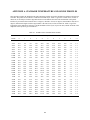
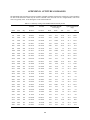
A.1
TOMS Version 7 Standard Ozone Profiles. . . . . . . . . . . . . . . . . . . . . . . . . . . . . . . . . . . . . . . . . . . . . . . . . . . . . 53
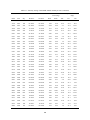
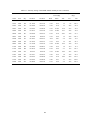
A.2
TOMS Version 7 Standard Temperature Profiles . . . . . . . . . . . . . . . . . . . . . . . . . . . . . . . . . . . . . . . . . . . . . . . . 54
A.3
Umkehr Layers. . . . . . . . . . . . . . . . . . . . . . . . . . . . . . . . . . . . . . . . . . . . . . . . . . . . . . . . . . . . . . . . . . . . . . . . . . 54
D.1
Summary Listing of TOMS Attitude Anomaly Events . . . . . . . . . . . . . . . . . . . . . . . . . . . . . . . . . . . . . . . . . . . 59
E.1
EP/TOMS Orbits with No Ozone Data . . . . . . . . . . . . . . . . . . . . . . . . . . . . . . . . . . . . . . . . . . . . . . . . . . . . . . . 63
E.2
Incomplete EP/TOMS Orbits. . . . . . . . . . . . . . . . . . . . . . . . . . . . . . . . . . . . . . . . . . . . . . . . . . . . . . . . . . . . . . . 63
E.3
EP/TOMS Orbits Containing Stare Mode Data . . . . . . . . . . . . . . . . . . . . . . . . . . . . . . . . . . . . . . . . . . . . . . . . . 64
vi
1.0 INTRODUCTION
This document is a guide to the data products derived from the measurements made by the Earth Probe Total Ozone
Mapping Spectrometer (EP/TOMS), and processed by the National Aeronautics and Space Administration (NASA).
It discusses the calibration of the instrument, the algorithm used to derive ozone values from the measurements,
uncertainties in the data, and the organization of the data products. The data begin July 25, 1996 and are ongoing at
the time of this publication. These data are being archived at the Goddard Space Flight Center (GSFC) Distributed
Active Archive Center (DAAC), and being made available in near real-time based on preliminary calibration through
the TOMS Web site as given in Appendix C.
The EP/TOMS was launched only a few months before another TOMS Instrument was launched aboard ADEOS, a
Japanese meteorological satellite. The EP/TOMS was put in a lower, 500 km orbit in order to provide higher spatial
resolution for studies of local phenomena. After failure of the ADEOS satellite on June 29, 1997, it was decided to
raise the EP/TOMS orbit to 750 km to provide more complete global coverage. This was accomplished over the
course of two weeks from December 4 through December 12 of 1997 during which no EP/TOMS data are available.
The result is an EP/TOMS data set of one and one half years of high resolution data taken at the expense of full global
coverage, and a continuing data set beginning in December of 1997 that provides more nearly global coverage. This
data set can be used for monitoring of long-term trends in total column ozone as well as seasonal chemical depletions
in ozone occurring in both southern and northern hemisphere polar spring. Other monitoring capabilities include
detection of smoke from bio-mass burning, identification of desert dust and other aerosols as well sulfur-dioxide and
ash emitted by large volcanic eruptions. A one and one half year gap exists in the long-term TOMS data record
between the failure of the Meteor-3 Spacecraft in December of 1994 and the beginning of the EP/TOMS data record
in July of 1996. In spite of this, the EP/TOMS data set represents a continuation of the TOMS dataset based on the
Nimbus-7 and Meteor-3 TOMS from October 31, 1978 through December 28, 1994, and on EP/TOMS from July 15,
1996 into the future. A follow-on TOMS experiment is scheduled to fly aboard a Russian Meteor-3M Spacecraft
planned to be launched in August of 2000.
The EP/TOMS is the first of three instruments built by Orbital Sciences Corporation to continue the TOMS Mission.
These instruments are similar in design to the previous TOMS instruments. They provide enhanced systems to
monitor long-term calibration stability, and a redefinition of two wavelength channels to aid in calibration monitoring
and to provide increased ozone sensitivity at very high solar zenith angles. One of the other new TOMS was flown
aboard the Japanese meteorological satellite, ADEOS, and the other is scheduled for launch aboard a Russian Meteor
Spacecraft in August of 2000. Further discussion of the EP/TOMS instrument is provided in Sections 2.1 and 3.
The EP/TOMS was the only instrument aboard an Earth Probe Satellite launched on July 2, 1996. It achieved its
initial orbit about 12 days later, and began taking measurements on July 15th. The EP/TOMS measures solar
irradiance and the radiance backscattered by the Earth's atmosphere in six selected wavelength bands in the
ultraviolet. It scans the Earth in 3-degree steps to 51 degrees on each side of the subsatellite point in a direction
perpendicular to the orbital plane.
The algorithm used to retrieve total column ozone (also referred to as total ozone) from these radiances and
irradiances is outlined in Section 2.2 and described in detail in Section 4. This algorithm is identical to the one used
for the Version 7 Nimbus–7 and Meteor-3 TOMS data archive. Because of this, the initial archive of the EP/TOMS
data set is also referred to as Version 7. A radiative transfer model is used to calculate backscattered radiances as a
function of total ozone, latitude, viewing geometry, and reflecting surface conditions. Ozone can then be derived by
comparing measured radiances with theoretical radiances calculated for the conditions of the measurement and
finding the value of ozone that gives a computed radiance equal to the measured radiance.
Section 2 provides a general overview of the EP/TOMS instrument, the algorithm, the uncertainties in the results, and
of other basic information required for best use of the data files. It is designed for the user who wants a basic
understanding of the products but does not wish to go into all the details. Such a user may prefer to read only those
parts of Sections 3 through 6 addressing questions of particular interest. In Section 3, the instrument, its calibration,
and the characterization of its changes with time are discussed. The algorithm for retrieval of total ozone and its
theoretical basis are described in Section 4. Section 5 describes the overall uncertainties in the ozone data and how
1
they are estimated, while Section 6 discusses particular problems that may produce errors in specific time intervals
and geographical areas. Both sections identify some anomalies remaining in the data and discuss what is known
about them. The structure of the data products is identical to those of previous TOMSs. This information is presented
in Section 7. Appendix A tabulates the standard atmospheric ozone and temperature profiles used in the algorithm
for ozone retrieval. Appendix B describes software available for reading the data files, and Appendix C provides
information on data availability. Appendix D contains a catalog of Earth Probe Spacecraft attitude anomalies that
affect the derived ozone at off-nadir scan positions by less than 1%.
2
2.0 OVERVIEW
2.1
Instrument
EP/TOMS was the only instrument aboard an Earth Probe satellite launched by a Pegasus XL rocket on July 2, 1996.
The satellite reached its initial orbit of 500 km at an inclination 98 degrees and a local equator crossing time of 11:16
AM some 12 days later, and regular ozone measurements began on July 25. The EP/TOMS experiment provides
measurements of Earth’s total column ozone by measuring the backscattered Earth radiance in the six 1-nm bands
listed in Table 3.1. The experiment uses a single monochromator and scanning mirror to sample the backscattered
solar ultraviolet radiation at 35 sample points at 3-degree intervals along a line perpendicular to the orbital plane. It
then quickly returns to the first position, not making measurements on the retrace. Eight seconds after the start of the
previous scan, another scan begins. The measurements used for ozone retrieval are made during the sunlit portions of
the orbit. In December of 1997, the EP/TOMS orbit was elevated to an altitude of 739 km with an inclination of
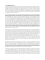
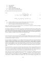
98.4°. The local equator crossing time was unchanged. Figure 2.1 illustrates the resulting instantaneous fields of view
(IFOV) on the Earth’s surface for adjacent scans and adjacent orbits. In its initial operation, the scanner measured 35
scenes, one for each scanner view angle stepping from right to left. The lower orbit was selected to provide the higher
spatial resolution shown in Figure 2.1 at the expense of inter-orbit filling which would provide daily global coverage.
Global coverage was not a concern until failure of the Japanese meteorological satellite, ADEOS which carried a
TOMS and provided that function. After the orbit elevation, EP/TOMS gives better coverage between orbits resulting
in 90% daily global coverage.
Figure 2.1 Earth Probe TOMS Instantaneous Fields of View Projected onto Earth's Surface. The right portion
(samples 18-35) of two consecutive scans are shown, and a portion of a scan from the previous orbit is also shown to
illustrate the degree of inter-orbit coverage at the equator for: a) 500 km orbit altitude, and b) 750 km orbit altitude.
The higher orbit after December 1997, results in 90% daily global coverage (84% at equator and 100% at 30°
latitude).
The ozone retrieval uses a normalized radiance, the ratio of the backscattered Earth radiance to the incident solar
irradiance. This requires periodic measurements of the solar irradiance. To measure the incident solar irradiance, the
TOMS scanner is positioned to view one of three ground aluminum diffuser plates housed in a carousel. The selected
diffuser reflects sunlight into the instrument. The diffuser plate is the only component of the optical system not
3
common to both the Earth radiance and the solar irradiance measurement. Only a change in the reflectivity of the
diffuser plate can cause a change of the radiance/irradiance ratio with time. In principle, an accurate characterization
of these changes will yield the correct variation of this ratio, and hence, an accurate long-term calibration of the
instrument. The three diffuser plates are exposed at different rates, allowing calibration by examining the differences
in degradation of diffuser reflectivity resulting from the different rates of exposure. This approach was first used with
Meteor 3 TOMS (Jaross et al., 1995) and proved to be very successful. In addition, the EP/TOMS is equipped with
UV lamps for monitoring the reflectivity of the solar diffusers. A more detailed description of the instrument and its
calibration appears in Section 3.
2.2 Algorithm
Retrieval of total ozone is based on a comparison between the measured normalized radiances and radiances derived
by radiative transfer calculations for different ozone amounts and the conditions of the measurement. It is
implemented by using radiative transfer calculations to generate a table of backscattered radiance as a function of
total ozone, viewing geometry, surface pressure, surface reflectivity, and latitude. Given the computed radiances for
the particular observing conditions, the total ozone value can be derived by interpolation in radiance as a function of
ozone. It is also possible to reverse this process and use the tables to obtain the radiances that would be expected for
a given column ozone and conditions of the measurement. The logarithm of the ratio of this calculated radiance to the
measured radiance is the residue.
The reflecting surface is assumed to consist of two components, a surface component of lower reflectivity and a cloud
component of higher reflectivity. By comparing the measured radiance at the ozone-insensitive 360 nm wavelength
with that calculated for cloud and for ground reflection alone, the effective cloud fraction and the contribution from
each level can be derived. Using this effective cloud fraction and the radiances measured at one pair of wavelengths,
an initial ozone estimate is derived using the tables. This ozone estimate is then used to calculate the residues at all
TOMS wavelengths except the longest. A correction to the initial ozone estimate is then derived from the residues at
selected wavelengths. Applying this correction produces the Best Ozone value. The choice of wavelengths is based
upon the optical path length of the measurement. Section 4 provides a full description of the algorithm. The OPT has
developed algorithms for the derivation of other parameters from the TOMS measurements in addition to total ozone.
These include an estimate of UVB flux at the surface (Krotkov et al., 1998) and estimates of aerosol loading due to
the presence of atmospheric aerosols (Hsu et al., 1996; Seftor et al,. 1997; Herman et al., 1997; and Torres et al., 1995
and 1998a).
2.3 Data Uncertainties
Uncertainties in the ozone values derived from the TOMS measurements have several sources: errors in the
measurement of the radiances, errors in the values of input physical quantities obtained from laboratory
measurements, errors in the parameterization of atmospheric properties used as input to the radiative transfer
computations, and limitations in the way the computations represent the physical processes in the atmosphere. Each
of these sources of uncertainty can be manifested in one or more of four ways: random error, an absolute error that is
independent of time, a time-dependent drift, or a systematic error that will appear only under particular
circumstances. For EP/TOMS total ozone, the absolute error is ± 3 percent, the random error is ± 2 percent (though
somewhat higher at high latitudes) and the drift after 1.5 years of operation is less than ± 0.6 percent. More detailed
descriptions of the different sources of uncertainty and the extent to which each contributes to the overall uncertainty
appear in Sections 3, 5, and 6. Section 3 discusses uncertainties due to errors in the characterization of the instrument
sensitivity. Section 5 discusses other sources of random errors, absolute error, and drift, combining them with the
instrument error to yield the overall estimates given above. Section 6 discusses errors that are limited in their scope to
specific times, places, and physical conditions. Sections 5 and 6 also describe the remaining anomalies that have been
identified in the EP/TOMS data set, with a discussion of what is known of their origin.
Comparisons between EP/TOMS and ground based measurements of total ozone indicate that the EP/TOMS data are
consistent with these uncertainties. The EP/TOMS ozone is approximately 1.0% higher than a 30 station network of
ground measurements. Nimbus-7 TOMS is about 0.5% higher than a similar ground based network (McPeters and
4
Labow, 1996) and Meteor-3 TOMS is not significantly different from the same network. None of the TOMS ozone
data sets show any significant drift relative to the ground based networks.
Data quality flags are provided with the derived ozone in the TOMS Ozone File (Level–2 data product). Only the
data quality flag values of 0 are used to compute the averages provided on the CDTOMS (Level–3) product. Other
flag values indicate retrieved ozone values that are of lower quality, allowing the users of Level–2 to decide whether
or not they wish to accept such data for their applications.
2.4 Archived Products
The EP/TOMS total ozone products are archived at the GSFC DAAC in Hierarchical Data Format (HDF). There are
two kinds of total ozone products: the TOMS Ozone File or Level-2 Data Product, and the CDTOMS or Level-3 Data
Product. The TOMS Ozone File contains detailed results of the TOMS ozone retrieval for each IFOV in time
sequence. One file contains all the data processed for a single orbit. The CDTOMS contains daily averages of the
retrieved ozone and effective surface reflectivity in a 1-degree latitude by 1.25-degree longitude grid. In areas of the
globe where orbital overlap occurs, the view of a given grid cell closest to nadir is used, and only good quality
retrievals are included in the average. Detailed descriptions of these products are provided in Section 7. Each
CDTOMS file contains one daily TOMS map (0.4 megabyte/day).
2.5 Near Real-Time Products
The EP/TOMS Level-3 data are also made available in near real-time over the internet. The near real-time products
are not to be considered of the same high quality as those available through the archive, but they can be accessed
earlier through the EP/TOMS Web Site at “http://jwocky.gsfc.nasa.gov/eptoms/ep.html”.
5
3.0 INSTRUMENT
3.1 Description
The TOMS on board the Earth Probe satellite measures incident solar radiation and backscattered ultraviolet sunlight.
Total ozone was derived from these measurements. To map total ozone, TOMS instruments scan through the subsatellite point in a direction perpendicular to the orbital plane. The Earth Probe TOMS instrument is identical to two
other new TOMS instruments, one of which was flown aboard the Japanese Meteorological Satellite ADEOS I in
1996, the other is scheduled for launch aboard a Russian Meteor Spacecraft in August of 2000. These three are
essentially the same as the first two TOMS, flown aboard Nimbus 7 and Meteor 3: a single, fixed monochromator,
with exit slits at six near-UV wavelengths. The slit functions are triangular with a nominal 1-nm bandwidth. The
order of individual measurements is determined by a chopper wheel. As it rotates, openings at different distances
from the center of the wheel pass over the exit slits, allowing measurements at the different wavelengths. The order is
not one of monotonically increasing or decreasing wavelength; two samples at each wavelength are interleaved in a
way designed to minimize the effect of scene changes on the ozone retrieval. The Instantaneous Field of View (IFOV)
of the instrument is 3 degrees x 3 degrees. A mirror scans perpendicular to the orbital plane in 3-degree steps from 51
degrees on the left side of spacecraft nadir to 51 degrees on the right (relative to direction of flight), for a total of 35
samples. At the end of the scan, the mirror quickly returns to the first position, not making measurements on the
retrace. Eight seconds after the start of the previous scan, another begins.
On previous TOMS consecutive cross scans overlapped, creating a contiguous mapping of ozone. The low altitude of
EP/TOMS (500 km) meant less overlap for EP/TOMS than for N7/TOMS (935 km), or M3/TOMS (1050 km), or
ADEOS TOMS (800 km). Overlap occurred poleward of 50 degrees. The initial mean localtime of the ascending
node was 11:16 AM, and remained in the range from 11:03 AM to 11:30 AM throughout the first year. The orbital
inclination was 97.55 deg. and remained essentially unchanged until the orbit was raised. Orbital altitude was 500
km, decaying to 495 km after 1 year. This translates to an orbital period of 94 min. 44 sec. at launch. Between
December 4th and 12th of 1997, the Earth Probe orbit was raised to a mean altitude of 739 km. The new orbital
period is 99.7 min. and has a 98.4° inclination. The time of the ascending node is essentially unchanged.
One significant difference in the new TOMS series from the previous Nimbus-7 and Meteor 3 TOMS is a change in
the wavelength selection for the 6 channels of the three new instruments. Four of the nominal band center
wavelengths (Table 3.1) remain the same on all TOMS. Channels measuring at 340 nm and 380 nm have been
eliminated in favor of 309 nm and 322 nm on the new TOMS. Ozone retrieval at 309 nm is advantageous because of
the relative insensitivity to calibration errors, though retrievals are limited to equatorial regions. Ozone retrievals at
high latitudes are improved because 322 nm is a better choice for the optical paths encountered there.
Backscatter ultraviolet instruments measure the response to solar irradiance by deploying a ground aluminum diffuser
plate to reflect sunlight into the instrument. Severe degradation of the Nimbus–7 diffuser plate was observed over its
14.5 year lifetime, and determining the resultant change of the instrument sensitivity with time proved to be one of
the most difficult aspects of the instrument calibration (Cebula et al., 1988; Fleig et al., 1990, Herman et al., 1991;
McPeters et al., 1993; Wellemeyer et al., 1996). The three-diffuser system aboard Meteor–3 and subsequent TOMS
reduces the exposure and degradation of the diffuser used for the solar measurements and allows calibration through
comparison of signals reflected off diffusers with different rates of exposure. The diffusers, designated Cover,
Working, and Reference, are arranged as the sides of an equilateral triangle and mounted on a carousel, so that a given
diffuser can be rotated into view on demand. The Reference diffuser is normally exposed for one sequence every 5
weeks, the Working diffuser every week, and the Cover diffuser is exposed for the remainder of the time whether or
not the solar flux is being measured. Comparison of the solar irradiance measurements from the different diffusers is
used to infer that the degradation of the Reference diffuser on EP/TOMS was negligible during the initial low orbit
period.
A new feature on EP/TOMS is the ability to monitor solar diffuser reflectance. A device referred to as the
Reflectance Calibration Assembly (RCA) was added to the new series of TOMS. This assembly employs a phosphor
light source with peak emission over the TOMS wavelength range. When powered on, the lamp illuminates the
exposed diffuser surface which is then viewed using the TOMS scan mirror. The scan mirror also rotates to view the
6
phosphor surface directly. The ratio of signals in the two scan mirror positions is a measure of relative diffuser
reflectance.
The EP/TOMS has eleven operating modes during normal operations. The most important of these are:
1. Standby mode
2. Scan mode
3. Solar calibration mode
4. Wavelength monitoring mode
5. Electronic calibration mode
6. Reflectance calibration mode
7. Direct control mode
The primary operating mode of the TOMS is scan mode. It is in this mode that the scanning mirror samples the 35
scenes corresponding to the scanner view angles, measuring the backscattered Earth radiances used for deriving column ozone. During the nighttime portion of the orbit the instrument is placed in standby mode, at which time the scan
mirror points into the instrument at a black surface. During solar calibration mode the scanner moves to view the exposed diffuser surface. The remaining modes are specialized for calibration purposes as the names indicate. The direct
control mode was also used several times in early 1997 to stop instrument scanning and make a continuous series of
measurements along a single ground track.
3.2 Radiometric Calibration
Conceptually, the calibration of the TOMS measured Earth radiance and solar irradiance may be considered
separately. The Earth radiance can be written as a function of the instrument counts in the following way:
I m ( t ) = C r k r G r f inst ( t )
(1)
where
Im(t )
Cr
kr
Gr
f inst
=
=
=
=
=
derived Earth radiance,
counts detected in earth radiance mode,
radiance calibration constant,
gain range correction factor, and
correction for instrument changes.
The measured solar irradiance, F m can be written as:
F m ( t ) = C i k i G i f inst ( t ) / gρ ( t )
(2)
where
Ci
ki
Gi
f inst
ρ(t )
g
=
=
=
=
=
=
irradiance mode counts,
irradiance calibration constant,
gain range correction factor,
correction for instrument changes,
solar diffuser plate reflectivity ( ρ (t = 0) = 1), and
relative angular correction for diffuser reflectivity.
In practice, however, there is no attempt to accurately determine kr or ki separately, either their absolute value or time
dependent changes. The primary quantity measured by TOMS and used to derive ozone is the normalized radiance,
7
I m ⁄ F m . The advantage of this approach is that the spectrometer sensitivity changes affecting both the Earth and solar
measurements ( f inst ) cancel in the ratio.
The ratio becomes:
Cr Gr
Im
-------- = ------ K ------gρ ( t )
(3)
Ci Gi
Fm
where K is a combined calibration constant for TOMS normalized radiances referred to as the albedo calibration
constant (Table 3.1). Radiance and irradiance measurements are generally made in different gain ranges, but evidence
indicates that G has been properly characterized (see Section 3.4). The initial absolute TOMS calibration therefore,
involves knowledge of the quantity krg/ki. Since the instrument changes affecting both the Earth and solar
measurements cancel in the ratio, the quantity critical to the time-dependent calibration of the normalized radiance is
the diffuser plate reflectivity, ρ(t). The angular dependence, g, is primarily required to correct for the diffuser Bidirectional Reflectivity Distribution Function (BRDF), but also contains the small correction due to light scattered
from the instrument.
Table 3.1.Earth Probe TOMS Albedo Calibration Constants and Gain Range Ratios.
Wavelength
(nm)
Adjustment Factor
(ratio)
Albedo Cal Constant
(steradian-1)
308.60
0.087
1.015
313.50
0.088
1.015
317.50
0.089
1.012
322.30
0.088
1.010
331.20
0.091
1.009
360.40
0.094
1.000
Gain Range Ratios
3.2.1
Range 2/1
Range 3/2
10.027
9.999
Prelaunch Calibration
Earth Probe TOMS prelaunch characterization included determination of the albedo calibrations, K, and band center
wavelengths. Both of these are reported in Table 3.1. Several different methods were employed to measure the values
of K for the six TOMS channels. These included separate characterization of radiance and irradiance sensitivity and
direct measurement of the flight diffuser reflectance. Only one method was chosen to represent the instrument
calibration.
The technique selected to calibrate the instrument radiance and irradiance sensitivity ratio (albedo calibration)
involves calibration transfer from a set of laboratory diffuser plates. These Spectralon diffusers were independently
characterized by GSFC and by NIST. A NIST-calibrated tungsten-halogen lamp is used to illuminate a Spectralon
plate which in turn is viewed by the instrument. This yields an estimate of the radiance calibration constants kr. The
same lamp illuminating the instrument directly yields the irradiance calibration constants ki. In the ratio of calibration
constants many systematic error sources, such as absolute lamp irradiance, cancel. The value of ki is also measured at
various illumination angles to determine the angular correction g.
The film strip technique was used to determine instrument wavelength selection. Photo-sensitive film is placed to
cover the six exit slits prior to final instrument assembly. An image of the exit slits is obtained by exposing the film
with the slit plate acting as a mask. The film is then exposed through the monochromator using several emission line
sources placed at the entrance slit of the instrument. The film images of these lines overlap the exit slit images, thus
8
providing for relative measurement of the two. Several films are used to provide optimum exposure and to give the
best estimate for band centers.
A reassessment of the film strip data from ADEOS TOMS revealed a deviation from the nominal band center
wavelength of the 312.5 nm and 360 nm channels of 0.02 nm and 0.3 nm respectively. These errors were determined
by comparing the slit position on the film with positions of nearby emission lines. A similar analysis performed for
the EP/TOMS film strip data yielded a 0.3 nm error in the 360 nm channel, but no error at 312.5 nm. No adjustment
has been applied to the data to account for the 360 nm error. A 0.3-0.4 N-value error in the aerosol index results, and
derived ozone is systematically high by approximately 0.5%. This ozone error is reflected in the time invariant
wavelength calibration uncertainty in Table 5.1.
3.2.2
Radiance-Based Calibration Adjustments
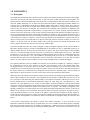
The initial albedo calibrations of the wavelengths were adjusted prior to processing. The main motivation for this
adjustment is algorithmic. Since different wavelengths are used to determine total ozone in different solar zenith
angle regimes, it is imperative that the wavelength dependence of the initial calibration be consistent with the forward
model calculation of the theoretical radiances used in the retrieval. Any inconsistencies can be identified through
analysis of the residues (see Section 4.5 for further discussion of the residues). In cases where the A-triplet (313 nm,
331 nm, and 360 nm) wavelengths are used to determine total ozone and effective reflectivity, adjusted residues can
be computed for the remaining wavelengths (309 nm, 318 nm, and 322 nm). These residues specifically characterize
the inconsistency of the measured radiances with the total ozone and reflectivity derived using the A-triplet. Modal
residues to A-triplet retrievals from the equatorial region were used to estimate the necessary adjustments (see Table
3.1). No adjustment has been made to the absolute scale (360 nm albedo calibration value). Since these adjustments
were based on data from the first few days of operation, some small inconsistencies remain, on average, in the data
(Figure 4.1), but these are well within the error budget discussed in Section 5.
3.2.3 Time-Dependent Calibration
As discussed in the introduction to this section, the time-dependent calibration requires a correction for changes in the
reflectivity of the solar diffuser plate. The EP TOMS was equipped with a carousel with three diffusers that were
exposed to the degrading effects of the Sun at different rates. The cover diffuser was exposed almost constantly, but
the working diffuser was exposed weekly, and the reference diffuser was exposed once every 5 weeks. While the
cover diffuser degraded quite rapidly, working and reference diffuser degradation has been minor.
Evidence for Working surface reflectance change has been observed through comparison of working and reference
solar signals. By assuming that reflectance change is proportional to solar exposure amount we have estimated the
total reflectance decrease in the working surface. Decreases at the end of 1997 relative to the initial values were 0.7%
and 1.0% at 360 nm and 309 nm, respectively. The uncertainty is + 0.1%. However, the decreases scale linearly with
wavelength. Therefore, changes in triplet wavelength combinations are insignificant at the level of 0.1% (see
discussion in Section 4.5). As a consequence, we have not applied a correction to existing data to account for diffuser
degradation. We treat all solar data from the working surface as though its reflectance has remained constant.
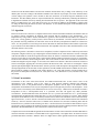
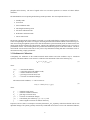
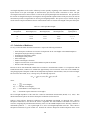
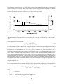
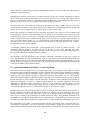
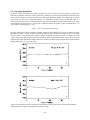
Solar measurements are made near the northern terminator when the trailing side of the spacecraft and the TOMS
solar diffuser carousel are exposed to the sun. Weekly measurements of the Working surface are presented in Figure
3.1, where the initial values have been normalized to 1 and signals have been corrected for sun/earth distance. These
plots represent finst (equation 2) since we have assumed no degradation of the Working surface. In the figure, the 360
nm signal is shown along with the 331/360 nm signal ratio and the A triplet wavelength combination. The nearly 25%
decrease at 360 nm is substantial, greater than previous TOMS instruments. The decrease in throughput is believed to
be optical degradation of the fore-optics, probably the scan mirror. A curious feature is observed in ratios to the 360
nm channel, and exemplified by the 331/360 nm plot. The rate of decrease in instrument throughput was initially
greater at shorter wavelengths, but reversed after 6 months. The reasons for this are not completely understood. It
appears to be the result of two competing changes, one where sensitivity decrease is greater at short wavelengths and
one where it is greater at long wavelengths.
9
Figure 3.1. Estimated Change in EP/TOMS Instrument Sensitivity Based on Solar Measurements Using the Working
and Reference Diffusers. Working diffuser solar measurements (+), and fit characterizations used in the archive
processing (solid line) are shown.
10
The solar Working measurements have been used to characterize the instrument calibration for the near real-time
product. Since Cr and Ci of equation 3 cannot be measured simultaneously, Ci must be characterized at the time at
which Cr are measured. A regression of existing solar data is performed every week to predict the value of Ci for the
coming week. These predictions are shown overplotted in Figure 3.1. In near real-time mode, the regression changes
each week with the addition of new data, so small weekly discontinuities result. Also, regressions are performed for
360 nm and the five wavelength ratios to that channel. This results in a somewhat poorer prediction for the triplet
combinations, the characterizations which most affect ozone. Deviations typically do not exceed 0.3% in equivalent
ozone.
The earth radiance data from 1996 have been reprocessed. The characterization of Ci used for this reprocessing was
based on a smooth polynomial regression of the 1996 solar data. The near real-time predictions described above begin
in 1997. The EP TOMS data are being archived in this form in 1998, and may be reprocessed using a smooth function
later in the life of the mission.
3.3
Wavelength Monitoring
Following the laboratory wavelength calibration, an on-board wavelength monitor has tracked changes in the
wavelength scale, both before launch and in orbit. Change might be produced by excessive temperature differentials
or mechanical displacement of the wavelength-determining components resulting from shock or vibration. Scans of
an internal mercury-argon lamp for in-flight monitoring of the wavelength selection are executed once per week
during nighttime. The wavelength calibration is monitored by observing two wavelength bands on either side of the
296.7-nm Hg line. Relative changes in the signal level indicate wavelength shifts. These shifts are nearly equivalent at
all 6 wavelengths. There is no evidence of any prelaunch wavelength drift. Wavelength monitor results indicate a drift
in band centers since launch of less than 0.02 nm. Changes in the instrument wavelength selection of this magnitude
are not considered significant for ozone retrieval.
3.4
Gain Monitoring
The current from the Photo-Multiplier Tube (PMT) is fed to three electronic amplifiers in parallel, each of which
operates in a separate gain range. The choice of amplifier recorded for output is based upon the signal level. Thus,
knowledge of the gain ratios between ranges represents part of the determination of instrument linearity, and the
stability of the gain ratios can affect the time-dependent calibration of the normalized radiance (Equation 3). The two
ratios were determined electronically prior to launch. The value of the ratios directly affects the ozone retrieval
because the solar calibration takes place exclusively in the least sensitive range, while earth measurements occur in all
three ranges.
In the postlaunch phase, the gain ratios are monitored using signals which are simultaneously amplified in all three
ranges. These simultaneous readings are reported in the instrument telemetry for one scene each scan. Thus earth
radiances can be used to verify the interrange ratios when the signals fall within the operating range for both
amplifiers. This tends to occur near the day/night terminator in the orbit. Interrange ratios have been found to be
constant in time, with average values close to the prelaunch characterization. The postlaunch averages used in ozone
processing are reported in Table 3.1.
3.5
Attitude Determination
The spacecraft attitude has been well maintained since launch. Apparent large excursions (up to 40 deg.) have been
observed in the horizon sensor, but these individual measurements do not represent true attitude changes and are
averaged for 16 sec before being used for attitude adjustment. These excursions occurred several times per month on
average during the low orbit period. They are believed to be caused by high energy particles creating noise in the
attitude sensor. Maximum errors in the actual attitude have been 0.6 deg. in roll and pitch, and the mean value was
about 0.1 deg. The errors arise when the spacecraft corrects for the perceived attitude error. Excursions always last
less than 2 minutes and occur throughout the orbit. Yaw excursions can be slightly larger (~1 deg. max.) and longer in
duration (~3 min.), but are correlated in time with roll/pitch changes. The effect of these attitude errors on solar
calculations is negligible. Errors in retrieved ozone resulting from altitude errors are typically 1 D.U. or less and are
always less the 4 D.U. These significant errors tend to be limited to the extreme off-nadir scenes. A table of orbits and
times when large attitude excursions occurred is given in Appendix D.
11
3.6
Validation
Several techniques are employed to validate characterizations of instrument performance. Among these is an internal
method based on the residues described in Section 4.5. Monitoring the triplet residue for the 309 nm channel is
equivalent to the pair justification method (Herman et al., 1991). This method is being used to verify wavelength
dependent changes in the spectrometer sensitivity, but cannot detect absolute changes at a single wavelength.
The spectral discrimination technique was first applied as the primary calibration technique for the Nimbus 7 TOMS,
which had no on-board diffuser calibration apparatus (Wellemeyer et al., 1996). This method has been applied to the
EP/TOMS data record. The trend in the 331 nm residue over highly reflective equatorial clouds indicates that the
wavelength dependent calibration of EP/TOMS is stable to within a few tenths of a percent. Using the spectral
discrimination technique, the difference in trend between the 331 nm residue over low reflecting surfaces and the 331
nm residue over highly reflective clouds can be used to derive the drift in calibration at the 360 nm reference channel.
This analysis indicates a small upward trend in derived surface reflectivity of approximately 0.5 percent over the first
1.5 years. This drift, which is consistent with our estimate of working diffuser degradation would have no significant
effect on derived ozone.
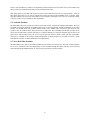
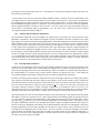
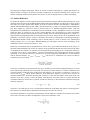
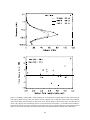
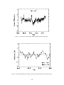
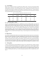
Absolute changes in spectrometer sensitivity have also been observed by studying signals measured at the nadir over
Antarctica and Greenland and corrected for solar zenith angle dependence. The ice signal time series is plotted with
the solar Working measurements in Figure 3.2. Greenland and Antarctica results have been combined in a single data
set by normalizing results during their overlap at the first equinox. Solar and ice data are further normalized to 1
during the first week of data. Ice results represent weekly average sensitivity values determined for all available
zenith angles up to 83 degrees. The solar and ice results at 360 nm exhibit good agreement, with deviations of less
than 1%.
Figure 3.2. Comparisons of estimates of instrument change in the EP/TOMS based on solar output and the
reflectivity of Antarctica and Greenland.
12
4.0 ALGORITHM
The Earth Probe TOMS algorithm is based on the one used for Nimbus-7 and Meteor-3 TOMS. The major differences
concern the use of the 360 nm wavelength for reflectivity instead of 380 nm and the use of 322 nm and 331 nm in the
C-triplet instead of 331 nm and 340 nm for ozone determination. The Earth Probe and ADEOS TOMS algorithms are
identical except for small differences in the band center wavelengths.
4.1 Theoretical Foundation
To interpret the radiance measurements made by the TOMS instrument requires an understanding of how the Earth’s
atmosphere scatters ultraviolet radiation as a function of solar zenith angle. Incoming solar radiation undergoes
absorption and scattering in the atmosphere by atmospheric constituents such as ozone and aerosols and by Rayleigh
scattering. Radiation that penetrates to the troposphere is scattered by clouds and aerosols, and radiation that reaches
the ground is scattered by surfaces of widely varying reflectivity.
The backscattered radiance at a given wavelength depends, in principle, upon the entire ozone profile from the top of
the atmosphere to the surface. The three shortest wavelengths used in the TOMS ozone measurements were selected
because they are strongly absorbed by ozone. At these wavelengths, absorption by other atmospheric components is
negligible compared to that by ozone.
At all of the TOMS wavelengths, the backscattered radiance consists primarily of solar radiation that penetrates the
stratosphere and is reflected back by the dense tropospheric air, clouds, aerosols, and the Earth’s surface. The
intensity is determined primarily by the total optical depth above the scattering layer in the troposphere. The amount
of ozone below the scattering layer is small and can be estimated with sufficient accuracy to permit derivation of total
column ozone. Because most of the ozone is in the stratosphere, the principal effect of atmospheric ozone at these
wavelengths is to attenuate both the solar flux going to the troposphere and the component reflected back to the
satellite.
Derivation of atmospheric ozone content from measurements of the backscattered radiances requires a treatment of
the reflection from the Earth’s surface and of the scattering by clouds and other aerosols. These processes are not
isotropic; the amount of light scattered or reflected from a given scene to the satellite depends on both the solar zenith
angle and view angle, the angle between the scene and the nadir as seen at the satellite.
Earlier TOMS algorithms, previous to the current version 7 algorithm, were based on the treatment of Dave (1978),
who represented the contribution of clouds and aerosols to the backscattered intensity by assuming that radiation is
reflected from a particular pressure level called the “scene pressure,” with a Lambert-equivalent “scene reflectivity”
R. When this method was applied, at the non-ozone-absorbing wavelengths the resulting reflectivity exhibited a
wavelength dependence correlated with partially clouded scenes. To remove this wavelength dependence, a new
treatment has been developed, based on a simple physical model that assumes two separate reflecting surfaces, one
representing the ground and the other representing clouds. The fractional contribution of each to the reflectivity is
obtained by comparing the measured radiances with the values calculated for pure ground and pure cloud origin.
The calculation of radiances at each pressure level follows the formulation of Dave (1964). A spherical correction for
the incident beam has been incorporated, and Version 7 treats molecular anisotropy (Ahmad and Bhartia, 1995).
Consider an atmosphere bounded below by a Lambertian reflecting surface of reflectivity R. The backscattered
radiance emerging from the top of the atmosphere as seen by a TOMS instrument, Im, is the sum of purely
atmospheric backscatter Ia, and reflection of the incident radiation from the reflecting surface Is,
I m ( λ, θ, θ 0, Ω, P 0, R ) = I a ( λ, θ, θ 0, φ, Ω, P 0 ) + I s ( λ, θ, θ 0, φ, Ω, P 0, R )
where
λ
θ
= wavelength,
= satellite zenith angle, as seen from the ground,
13
(4)
θ0
φ
Ω
P0
R
=
=
=
=
=
solar zenith angle,
azimuth angle,
column ozone amount,
pressure at the reflecting surface, and
effective reflectivity at the reflecting surface.
The surface reflection term can be expressed as follows:
where
RT (λ,θ, θ 0, Ω, P 0)
I s ( λ,θ, θ 0, Ω, P 0, R) = ----------------------------------------------1 – RS b (λ,Ω, P 0)
and
T (λ,θ, θ 0, Ω, P 0) = I d (λ,θ, θ 0, Ω, P 0) f (λ,θ, Ω, P 0)
(5)
(6)
where
Sb = fraction of radiation reflected from surface that atmosphere reflects back to surface,
Id = total amount of direct and diffuse radiation reaching surface at P0,
f = fraction of radiation reflected toward satellite in direction θ that reaches satellite,
and the other symbols have the same meaning as before. The denominator of Equation 5 accounts for multiple
reflections between the ground and the atmosphere.
The intensity of radiation as it passes through a region where it is absorbed and scattered can be described in general
terms as having a dependence I ∝ exp(-τ). For a simplified case, where all processes can be treated as absorption, the
optical depth τ depends on the number of absorbers n in a column and the absorption efficiency α of the absorbers;
that is, I ∝ exp(-nα). The column number should thus scale approximately as -log I. The ozone algorithm therefore
uses ratio of radiance to irradiance in the form of the N-value, defined as follows:
I
N = – 100 log 10  --- .
 F
(7)
The N-value provides a unit for backscattered radiance that has a scaling comparable to the column ozone; the factor
of 100 is to produce a convenient numerical range. (This same definition is used in the derivation of ozone from the
ground-based Dobson and Brewer networks).
The basic approach of the algorithm is to use a radiative transfer model to calculate the N-values that should be
measured for different ozone amounts, given the location of the measurement, viewing conditions, and surface
properties, and then to find the column ozone that yields the measured N-values. In practical application, rather than
calculate N-values separately for each scene, detailed calculations are performed for a grid of total column ozone
amounts, vertical distributions of ozone, solar and satellite zenith angles, and two choices of pressure at the reflecting
surface. The calculated N-value for a given scene is then obtained by interpolation in this grid of theoretical Nvalues.
The ozone derivation is a two-step process. In the first step, an initial estimate is derived using the difference between
N-values at a pair of wavelengths; one wavelength is significantly absorbed by ozone, and the other is insensitive to
ozone. Use of a difference provides a retrieval insensitive to wavelength-independent errors, in particular, any in the
zero-point calibration of the instrument. In deriving the initial estimate, the same pair is always used.
In the second step, N-values are calculated using this ozone estimate. In general, these calculated values will not
equal the measured N-values. The differences, in the sense Nmeas–Ncalc, are called the residues. Using the residues at
a properly chosen triplet of wavelengths, it is possible to simultaneously solve for a correction to the original ozone
estimate and for an additional contribution to the radiances that is linear with wavelength, arising primarily from
14
wavelength dependence in the surface reflectivity but also possibly originating in the instrument calibration. The
triplet consists of two pair wavelengths, as described above, plus 360 nm, which is insensitive to ozone. The pair
wavelengths used are those most sensitive to ozone at the optical path length of the measurement. The separation of
the 360-nm wavelength from the pair wavelengths is far larger than the separation between the pairs; thus, the 360-nm
measurement provides a long baseline for deriving wavelength dependence. This process may be iterated, using the
results of the first triplet calculation as the new initial estimate. Table 4.1 lists the wavelengths of the pairs and triplets.
Table 4.1. Pair/Triplet Wavelengths
Pair/Triplet
Designation
Ozone Sensitive
Wavelength (nm)
Ozone Insensitive
Wavelength (nm)
Reflectivity
Wavelength (nm)
Range of Application
(optical path s)
A
312.6
331.3
360.4
1≥s
B
317.6
331.3
360.4
3≥s>1
C
322.4
331.3
360.4
s>3
4.2 Calculation of Radiances
To carry out the calculation described in Section 4.1 requires the following information:
•
•
•
•
•
•
•
•
Ozone absorption coefficients as a function of temperature for the wavelengths in the TOMS bandpasses.
Atmospheric Rayleigh scattering coefficients.
Climatological temperature profiles.
Climatological ozone profiles.
Solar zenith angle.
Satellite zenith angle at the IFOV.
Angle between the solar vector and the TOMS scan plane at the IFOV.
Pressure at the reflecting surface.
Because of the its finite bandwidth, TOMS does not measure a monochromatic radiance. For comparison with the
TOMS measurements, radiances are calculated at approximately 0.05-nm intervals across each of the TOMS slits,
using the appropriate absorption coefficient and temperature dependence (Paur and Bass, 1985) for each wavelength.
The I/F for the entire band, A(λ0), is then given by the following expression:
∫
∫
A ( λ 0 ) = A ( λ )F ( λ )S ( λ ) dλ/ F ( λ )S ( λ ) dλ
(8)
where
A(λ)
F(λ )
I(λ)
S(λ)
=
=
=
=
I(λ)
------------ at wavelength λ,
F(λ)
solar flux at wavelength λ,
earth radiance at wavelength λ, and
Instrument response function at wavelength λ.
The wavelength dependence of the solar flux is based on SOLSTICE measurements (Woods et al., 1996). This
detailed calculation replaces the effective absorption coefficients used in Version 6.
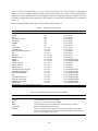
Table 4.2 shows effective absorption coefficients for the EP/TOMS wavelengths. As discussed above, effective
absorption coefficients are not used in the Version 7 algorithm. The same method of calculation was used as in
Version 6, integrating the monochromatic laboratory values over the TOMS bandpass for the following conditions: a
mid-latitude profile for Ω = 350, a path length of 2.5, and a wavelength-independent solar flux. These effective
absorption coefficients are given in Table 4.2. Because the effective absorption coefficient depends on the ozone
15
profile, optical path length, and solar flux spectrum, the Version 7 technique of calculating I/F at individual
wavelengths and then integrating over the TOMS bandpass eliminates the imprecision arising from using one set of
effective absorption coefficients, derived for a particular set of conditions, for all calculations. Table 4.2 also contains
the Rayleigh scattering coefficients and the regression equations used for the temperature dependence of the ozone
coefficients. The values shown in the table are purely to illustrate the magnitude of the change; they have not been
used in the algorithm.
Table 4.2. Effective Absorption and Scattering Coefficients
Vacuum Wavelength
(nm)
308.65
312.56
317.57
322.37
331.29
360.40
Effective Ozone
Absorption Coefficient
(atm-cm-1) at 0˚C
(C0)
Temperature Dependence
Coefficients
C1
C2
3.23
7.89 x 10-3
3.79 x 10-5
-3
1.83
6.10 x 10
3.15 x 10-5
-3
0.973
3.59 x 10
2.11 x 10-5
0.536
2.08 x 10-3
1.21 x 10-5
-4
4.94 x 10-6
0.165
9.10 x 10
-8
< 10
–
–
Correction to ozone absorption for temperature:
Ozone absorption = C0 + C1T + C2T2
(where T is in degrees C)
Rayleigh Scattering
Coefficient (atm-1)
1.077
1.020
0.953
0.894
0.795
0.557
Ozone and temperature profiles were constructed using a climatology based on SBUV measurements above 15 km
and on balloon ozonesonde measurements (Klenk et al., 1983) for lower altitudes. Each standard profile represents a
yearly average for a given total ozone and latitude. Profiles have been constructed for three latitude bands: low
latitude (15 degrees), mid-latitude (45 degrees), and high latitude (75 degrees). There are 6 profiles at low latitudes
and 10 profiles each at middle and high latitudes, for a total of 26. These profiles cover a range of 225–475 D.Us. for
low latitudes and 125–575 for middle and high latitudes, in steps of 50 D.Us. The profiles are given in Appendix A.
Differences between these assumed climatological ozone profiles and the actual ozone profile can lead to errors in
derived total ozone at very high solar zenith angles. The longer wavelength triplets are used at high path lengths
because they are much less sensitive to profile shape effects. The differential impact of the profile shape error at the
different wavelengths indicates, however, that profile shape information is present in the TOMS measurements at high
solar zenith angles. An interpolation procedure has been developed to extract this information (Wellemeyer et al.,
1997), and implement it in the Version 7 algorithm.
To use the new Version 7 ozone profile weighting scheme for high path lengths, it was necessary to extend the
standard profiles beyond the available climatology. To minimize the use of extrapolation in this process, profile
shapes were derived by applying a Principal Component Analysis to a separate ozone profile climatology derived
from SAGE II (Chu et al., 1989) and balloon measurements to derive Empirical Orthogonal Functions (EOFs). The
EOFs corresponding to the two largest eigenvalues represented more than 90 percent of the variance. The EOF with
the greatest contribution to the variance was associated with variation in total ozone. The second most important EOF
was associated with the height of the ozone maximum and correlated well with latitude, showing a lower maximum at
higher latitude. This correlation was used as the basis for lowering the heights of the ozone maxima at high latitudes
and raising them in the tropics when extending the original climatology to represent the more extreme profile shapes
(Wellemeyer et al., 1997).
Given the wavelength, total ozone and ozone profile, surface pressure, satellite zenith angle at the field of view, and
solar zenith angle, the quantities Im, Ia, T, and Sb of Equations 4 and 5 can then be calculated at the six TOMS
wavelengths. For the tables used in the algorithm, these terms are computed at the TOMS wavelengths for all 26
standard profiles and two reflecting surface pressure levels (1.0 atm and 0.4 atm). For each of these cases, Im, Ia, T are
calculated for 10 choices of solar zenith angle from 0–88 degrees, spaced with a coarser grid at lower zenith angles
16
and a finer grid for higher zenith angles, and for six choices of satellite zenith angle, five equally spaced from 0–60
degrees and one at 70 degrees. In Version 6, the tables extended only to a satellite zenith angle of 63.3 degrees. The
fraction of reflected radiation scattered back to the surface, Sb, does not depend on solar or satellite zenith angle.
4.3 Surface Reflection
To calculate the radiances for deriving ozone from a given measurement requires that the height and reflectivity of the
reflecting surface be known. The TOMS algorithm assumes that reflected radiation can come from two levels, ground
and cloud. The average ground terrain heights are from the National Oceanic and Atmospheric Administration
(NOAA) National Meteorological Center (NMC), provided in km for a 0.5-degree x 0.5-degree latitude and longitude
grid. These heights are converted to units of pressure using a U.S. Standard Atmosphere (ESSA, 1966) and
interpolated to the TOMS IFOVs to establish the pressure at the Earth’s surface. Probabilities of snow/ice cover from
around the globe are collected by the Air Force Global Weather Center and mapped on a polar stereographic
projection. These data have been averaged to provide a monthly snow/ice climatology mapped onto a 1-degree x 1degree latitude and longitude grid and used to determine the presence or absence of snow in the TOMS IFOV. If the
probability is 50 percent or greater, snow/ice is assumed to be present. For cloud heights, a climatology based upon
the International Satellite Cloud Climatology Project (ISCCP) data set is used. It consists of the climatological
monthly averages over a 0.5 x 0.5-degree latitude-longitude grid. The impact of the use of this climatology on the
TOMS derived ozone is discussed in Hsu et al., 1997.
Reflectivity is determined from the measurements at 360 nm. For a given TOMS measurement, the first step is to
determine calculated radiances at 360 nm for reflection off the ground and reflection from cloud, based on the tables
of calculated 360-nm radiances. For reflection from the ground, the terrain height pressure is used, and the reflectivity
is assumed to be 0.08. For cloud radiances, a pressure corresponding to the cloud height from the ISCCP-based
climatology is used, and the reflectivity is assumed to be 0.80. The ground and cloud radiances are then compared
with the measured radiance. If Iground ≤ Imeasured ≤ Icloud, and snow/ice is assumed not to be present, an effective
cloud fraction f is derived using
I measured – I ground
f = -------------------------------------------------------- .
I cloud – I ground
(9)
If snow/ice is assumed to be present, then the value of f is divided by 2, based on the assumption that there is a 50-50
chance that the high reflectivity arises from cloud. The decrease in f means that there is a smaller contribution from
cloud and a higher contribution from ground with a high reflectivity off snow and ice. Equation 9 is solved for a
revised value of Iground, and the ground reflectivity is calculated from Equation 5. For the ozone retrieval, the
calculated radiances are determined assuming that a fraction f of the reflected radiance comes from cloud with
reflectivity 0.80, and a fraction 1-f from the ground, with reflectivity 0.08 when snow/ice is absent and with the
recalculated reflectivity when snow/ice is present. An effective reflectivity is derived from the cloud fraction using the
following expression:
R = Rg ( 1 – f ) + Rc f
(10)
where Rg is 0.08 when snow/ice cover is assumed absent and has the recalculated value when it is assumed present.
This reflectivity is included in the TOMS data products but plays no role in the retrieval.
If the measured radiance is less than the ground radiance, then the radiation is considered to be entirely from surface
terrain with a reflectivity less than 0.08. Equations 4 and 5 can be combined to yield:
I – Ia
R = ----------------------------------- .
T + Sb ( I – I a )
17
(11)
The ground reflectivity can be derived using an Ia obtained assuming ground conditions. Similarly, if the measured
radiance is greater than the cloud radiance, when snow/ice are absent, the reflected radiance is assumed to be entirely
from cloud with reflectivity greater than 0.80, and an Ia derived using the cloud conditions is used in Equation 11 to
derive the effective reflectivity. If snow/ice are present, the cloud and ground are assumed to contribute equally to Im
at 360 nm. Equation 11 can then be used to calculate new values of both ground and cloud reflectivities from these
radiances. Radiances at the shorter wavelengths are calculated using these reflectivities and a value of 0.5 for f.
4.4 Initial B-Pair Estimate
The initial ozone is calculated using the B-pair, which provides good ozone values over the largest range of
conditions of any of the pairs.
The first step is to calculate radiances for the conditions of the measurement—geometry, latitude, cloud and terrain
height, and cloud fraction. For each ozone value in the table, radiances are calculated for the 1.0 atm and 0.4 atm
levels, using ground reflectivity and the values of Ia, T, and Sb from the tables for the geometry of the measurement
and a single ozone profile—the low latitude profile for measurements at latitudes 15 degrees and lower, the midlatitude profile for 15 degrees < latitude ≤ 60 degrees, and the high latitude profile at latitudes higher than 60 degrees.
These radiances are then corrected for rotational Raman scattering (the Ring effect). The correction factors, based on
the results of Joiner et al., (1995), are shown in Table 4.3. They were computed using a solar zenith angle of 45
degrees and a nadir scan. The dependences on solar and scan angles, which are small under most conditions, are
neglected. Two sets were calculated, one at 1 atm and the assumed 8 percent ground reflectivity for use with the 1-atm
radiance tables and the other at 0.4 atm and the assumed 80 percent cloud reflectivity for use with the 0.4-atm tables.
This correction greatly reduces the biases that had been seen between ozone values.
Table 4.3. Rotational Raman Scattering Corrections
Radiance Correction (%)
Actual Wavelength (nm)
308.65
312.56
317.57
322.37
331.29
360.40
Pressure = 1.0 atm
Reflectivity = 8%
–0.295
0.17
–0.598
0.126
0.310
–0.430
Pressure = 0.4 atm
Reflectivity = 80%
–0.167
0.006
–0.311
0.056
0.139
–0.175
The ground radiance is then derived by interpolating between values for the two pressures to derive the radiance for
the pressure at the terrain height from the grid. A similar process is carried out for both pressures using cloud
reflectivity, and the cloud radiance is derived by linear interpolation for the pressure level at the height given by the
ISCCP cloud height climatology. Finally, the appropriate fractions of ground and cloud radiances, determined as
described in Section 4.3, are added to yield I/F for all ozone values. These results are then converted to N-values.
The next step is to compare the measured radiance with the calculated radiance. The two tabulated ozone values
whose calculated B-pair N-value differences bracket the measured N-value difference are identified in the table. A
climatological ozone amount below the terrain pressure level is subtracted from these two bracketing table ozone
values, and the initial ozone estimate is derived by linearly interpolating between the two resultant values, using the
measured N-value and the two calculated N-values.
4.5 Best Ozone
Once an initial estimate of ozone has been obtained, it is used to calculate N-values at all TOMS wavelengths in the
way described in Section 4.2, applying the rotational Raman scattering correction described in Section 4.4. N-values
are calculated for each measurement, using one profile or two, depending upon the latitude. For latitude ≤ 15 degrees,
only the low latitude profiles are used, for 15 degrees< latitudes ≤ 45 degrees, one set each is calculated using low and
18
middle latitude profiles, for 45 degrees< latitudes < 75 degrees, N-values are calculated using middle and high
latitude profiles; and for latitude ≥ 75 degrees, only N-values for high latitude profiles are calculated. Values of dN/
dΩ are calculated, as well.
In general, these calculated N-values will not equal the measured N-values. In the derivation of the initial ozone
estimate, reflectivity is assumed to be independent of wavelength, but for some surface conditions, such as sea glint,
desert dust, or ice, the reflectivity will be wavelength dependent. In addition, residual errors in the instrument
calibration can produce a wavelength dependent artifact in the measured N-value. Because of these effects on the
spectrum of backscattered radiation and because of the simplifications used in its derivation, the initial ozone estimate
will not be equal to the true ozone value. This error in ozone will also contribute to the discrepancy between the
measured N-value Nm and the value N0 calculated from the initial ozone estimate. The initial ozone estimate should,
however, be sufficiently close to the true value to derive a correction using a first order Taylor expansion in the
difference. The wavelength-dependent contribution from factors other than ozone, such as reflectivity and residual
errors in the instrument characterization, is assumed to be a linear function of wavelength, a + bλ. Then,
dN
N m = N 0 + ( Ω – Ω 0 )  ------- + a + bλ .
 dΩ 0
(12)
Let
rλ
= (Nm –N0)λ be the residue at wavelength λ, and
sλ =  ------- be the sensitivity at wavelength λ.
dΩ λ
dN
Equation 17 becomes:
r λ = s λ ( Ω – Ω 0 ) + a + bλ .
(13)
The radiation at 360 nm is insensitive to ozone, and therefore s360 = 0. Further, since the reflectivity was derived at
360 nm, the residue is zero at that wavelength. Substituting into Equation 13 and solving yields:
a = – 360b
(14)
and therefore, for the ozone-sensitive wavelengths,
r λ = s λ ( Ω – Ω 0 ) + b ( λ – 360 ) .
(15)
There are two unknowns, Ω and b. Let ∆λ = λ-360. Using measurements at two wavelengths, labeled λ1 and λ2, it is
possible to solve for Ω:
r 1 ∆λ 2 – r 2 ∆λ 1
Ω = Ω 0 + --------------------------------------- .
s 1 ∆λ 2 – s 2 ∆λ 1
(16)
Equation 16 is the form in which the algorithm applies the correction. Ozone values are derived for each of the two
profiles selected.
Another form of this equation is:
∆λ 2 r 1 – s 1 ( Ω – Ω 0 )
---------- = ---------------------------------------- .
∆λ 1 r 2 – s 2 ( Ω – Ω 0 )
(17)
This form illustrates how the correction is equivalent to assuming that the size of that part of the residual not arising
from ozone error is linear with wavelength.
19
This situation is illustrated in Figure 4.1, which shows the modes of the equatorial distributions of residues at each
channel as a function of wavelength. These modal residues represent a huge population, but they serve to illustrate
concepts applicable to individual retrievals as well. Because the A-triplet is used exclusively at path lengths
encountered in the tropics, the modal residues at 313, 331, and 360 nm are co-linear.
Figure 4.1. Modes of Equatorial Distributions of Residues for Each of the EP TOMS Channels as a Function of
Wavelength. Residues are reported on the Level-2 product in units of N-value. A difference of 1 N-value is equal to
2.31%.
The A-triplet residue can be defined as:
λ - 360
r′ λ = r λ + ---------------------------- r 331 .
331 - 360
(18)
The modal A-triplet residues for the 309, 318, and 322 nm channels are equal to their vertical displacement from the
A-triplet line in Figure 4.1. These non-zero triplet residues indicate some residual wavelength dependent
inconsistency in the measurement system. This may be due to calibration error, some systematic error in the
atmospheric radiation transfer model used in the retrieval, or systematic wavelength dependence in the effective
surface reflectivity at the bottom of the atmosphere. As discussed in Section 3.2.2, calibration adjustments have been
made to remove the modal A-triplet residues. This is intended to remove the systematic offset that would occur
between A-triplet ozone and B-triplet or C-triplet ozone. It also serves to normalize the triplet residues for use in the
profile mixing scheme described below. As discussed in Section 3.2.2, these initial adjustments were derived based on
a limited population. Figure 4.1 is based on the first 1.5 years of data, so it represents the residual uncertainty in the
current archive dataset which is less than 1% in ozone. It also serves to illustrate the concept of A-triplet residue. Note
that similar definitions of B-triplet residue and C-triplet residue can be constructed relative to total ozone derived
using these triplets as well.
For retrievals at latitudes where two profiles are used, an ozone value appropriate to the latitude of the measurement is
then derived from the ozone values for the two profiles, using an equation of the following form:
Ω = ( 1 – f prof )Ω lower + f prof Ω higher
where
Ω
Ωlower
Ωhigher
fprof
=
=
=
=
best ozone,
ozone retrieved using lower latitude profile,
ozone retrieved using higher latitude profile, and
weight given to higher latitude profile.
20
(19)
Thus, fprof will be 0 if only the lower latitude profile is selected, 1 if only the higher latitude profile is selected, and in
between for a combination of the two profiles. The choice of pairs and fprof depends upon the optical path length
Ω0(sec θ0 + sec θ), in atm-cm.
For path lengths less than 1.5, a value of fprof obtained by simple linear interpolation in latitude,
latitude – latitude lower
f prof = -------------------------------------------------------------------------------------latitude higher – latitude lower
(20)
is used for latitudes between 15 and 75 degrees using the two profiles appropriate to the latitude. The low latitude
profile alone is used from the equator to 15 degrees, and the high latitude profile alone is used from 75 degrees to the
pole. For a path length less than or equal to 1.0, the A-triplet wavelengths are used in Equation 16; for a path length
greater than 1 and no greater than 1.5, the B-triplet is used with the same latitude interpolation.
For longer path lengths, the profile mixing scheme mentioned above in Section 4.2 is used to determine the profile
mixing factor, fprof. The basic principle is to improve the triplet ozone using profile shape information in the triplet
residue of a shorter wavelength to determine the profile mixing factor defining a linear combination of the standard
profiles that best explains the radiances at all four wavelengths. This profile mixing factor is defined as:
r′ ( lower )
f prof = ---------------------------------------------------------r′ ( lower ) – r ′ ( higher )
(21)
where lower and higher refer to latitudes of the two profiles used and r´ refers to the B-triplet residue for the 313 nm
channel for 1.5 < s < 3.0 and to the C-triplet residue at the 318 nm channel for s ≥ 3. In most cases, the appropriate
profile will be between the higher and lower latitude profiles, and the residues will be of opposite sign; thus the
denominator represents a distance between the residues (or sensitivity to profile shape) and the numerator a fraction
of this distance. When the low- and mid-latitude profiles are used, if the derived value of fprof is greater than 1, the
process is repeated using the mid- and high-latitude profiles; similarly, if fprof < 0 when using mid- and high-latitude
profiles, the process is repeated using the low- and mid-latitude profiles.
The final step is to estimate the amount of the derived ozone that is beneath clouds. Estimates of the ozone amount
under the cloud level pressure level are obtained for each of the two latitude profiles used to derive Best Ozone and
the two tabulated ozone values on either side of the derived Best Ozone. The column ozone beneath cloud is then
derived by interpolating in ozone and using fprof to weight the latitudes. Finally, this ozone amount is multiplied by
the cloud fraction f to derive the ozone in a particular field of view that is under cloud. The sensitivities are calculated
from the sensitivities for the two profiles using the same weighting as for ozone.
4.6 Validity Checks
The algorithm contains several validity checks for maintaining data quality. Before measured radiances are accepted
for use in ozone determination, the solar zenith angle, satellite attitude, and instrument status are checked to ensure
the suitability of the radiances and other geophysical input to the algorithm. This section describes the quality checks
performed to identify invalid and lower quality ozone values caused either by bad input data that passed
preprocessing checks or by limitations of the ozone algorithm. It also explains the significance of the error flags that
are set.
The principal tool used to investigate the validity and quality of a total ozone value is the set of residues. The residues
measure how well radiances calculated based on the ozone derived using one set of wavelengths match the radiances
measured at the other wavelengths. The usual significance of a large residue is that the atmospheric or surface
conditions deviate significantly from those assumed in the algorithm, for example, if reflectivity has a non-linear
dependence on wavelength. The final triplet residues for wavelengths used in the retrieval will be zero.
21
The first check is of all the non-zero residues; if any is greater than 12.5 in units of N-value, the error flag is set to 5.
This condition usually arises when problems in the data stream lead to incorrect values for the measured radiance or
when the atmospheric conditions are so unusual that the assumptions used in the calculation of radiances do not hold.
Data that pass flag 5 are checked for sulfur dioxide contamination. The SO2 index (SOI) is defined by the following
equation:
dN
dN
r = SOI ------------------- + ∆Ω  ------- + b ( λ – 360 ) .
 dΩ
d ( SO 2 )
(22)
This equation is formulated in the same way as Equation 13, the basic equation for the ozone correction, with an
additional term for sulfur dioxide contamination. The physical interpretation is that the mismatch between calculated
and measured radiance has a component due to SO2 in addition to the components due to ozone error, wavelengthdependent reflectivity, and residual calibration error accounted for in Equation 15. Using three wavelengths provides
three equations, which can be solved for SOI as a function of the residues, the sensitivities, and the wavelengths. The
algorithm uses the residues at 317 nm, 322 nm, and 331 nm. The 312-nm wavelength is not used because it is more
affected by aerosols. If the SOI is greater than 12.5, the error flag is set to 4. Since the triplet residues at the
wavelengths used to derive the SOI are all zero when the C-triplet is used to derive ozone with the B-triplet to select
the profile, SOI is not evaluated for path lengths greater than 3; the output data set will contain a fill value. SO2contaminated data will still be likely to be flagged by the remaining residue tests, but the presence of SO2 will not be
identified.
In principle, Equation 22 could be used to simultaneously solve for ozone and SOI. However, the wavelengths best
for ozone determination at a given path length are not necessarily the best for SOI determination. The more
complicated expression for ozone that would result would significantly increase the computer time required, and the
accuracy of the “corrected” ozone would likely be poor. For further information about SO2 derived from TOMS
measurements, see Krueger et al., 1995 and 1998, Schaefer et al., 1997, and Krotkov et al., 1997.
The next check assesses triplet consistency. If a single triplet is used, the triplet residue defined in Equation 18 is
checked for the ozone-sensitive wavelength not used in the ozone determination: 317 nm in the case of the A-triplet,
and 312 nm for the B-triplet. The maximum residues allowed, in N-value units, are 1.1 at 317 nm when an A-triplet
determination is checked and 0.9 at 312 nm when a B-triplet determination is checked. If a second triplet is used to
determine the profile, then the requirement is that a value of fprof can be found such that 0.5 ≤ fprof ≤ 3.5. Values of
fprof outside this limit require such a degree of extrapolation that the profile is not considered highly reliable. If the
data fail the relevant test, the error flag is set to 3. The next check uses the 331-nm residue. If this residue exceeds 4 in
N-value units, the error flag is set to 2. Flag values of 3 or 2 resulting from large residues imply that the values of I/F
may be inconsistent with the assumption that the linear correction can be used.
For solar zenith angles greater than 84 degrees, the algorithm loses accuracy. Most retrievals must make use of the Ctriplet, which is not highly sensitive to ozone. In addition, the conditions depart from those for which the radiative
transfer code was designed, in particular the extreme geometry (Caudill et al., 1997). For this case, the error flag is set
to 1. Finally, the value 10 is added to the flag value for the data that are taken in polar summer on the descending
(north to south) part of the orbit. While all flagged ozone values appear on the Level–2 data sets, only ozone values
with the flag set to 0 for a good retrieval from the ascending part of the orbit are used to derive the gridded means of
Level–3.
22
Table 4.4 summarizes the error flags, when they are set, and their significance.
Table 4.4. Error Flags
Flag
4
5
Criterion
No other flag set
Solar zenith angle > 84˚
r(331) > 4 (N-value)
rtrip(317) > 1.1 (N-value)
(if A-triplet alone used)
rtrip(312) > 0.9 (N-value)
(if B-triplet alone used)
fprof < -0.5 or fprof > 3.5
(profile selection)
SOI > 24
any residue > 12.5
+10
Descending orbit
0
1
2
3
Significance
Good value
Algorithm less accurate
Linear correction inadequate
Linear correction inadequate
Anomalous Profile
Sulfur dioxide contamination
Unusual atmospheric conditions or
data stream problems
Data taken during descending (north to
south) portion of orbit.
4.7 Level 3 Gridding Algorithm
The level-3 gridding algorithm is used to combine the orbital TOMS measurements into a daily map product with a
fixed global grid. The grid used is 1 degree in latitude by 1.25 degrees longitude over the entire globe. Only high
quality level-2 data with a quality flag of zero as defined in Table 4.4 are included in the cell averages.
The cell averages are computed as weighted averages of TOMS parameters derived for IFOVs that overlay the given
cell. For this purpose, a simple rectangular model is used for the actual TOMS IFOV, which is illustrated in Figure
2.1. The area of overlap between the rectangular IFOV and a given cell is used to weight its contribution to the given
grid cell average. A single TOMS IFOV can contribute weight to more than one cell average within a single 1 degree
latitude band. Contributions outside the latitude band are ignored as a simplification of the calculation. The
dimensions of the model IFOV vary from 26 km x 26 km at nadir to 45 km x 80 km at the extreme off-nadir for the
low 500 km orbit period, and from 38 km x38 km at nadir to 70 km x140 km at the extreme off-nadir during the high
750 km orbit period after December 12, 1996.
At higher latitudes where orbital overlap occurs, the orbit that provides the best view of a given cell is used. In
practice, cell averages are computed separately for each TOMS orbit, and the one with the shortest average path index
is selected. The path index is calculated as sec(θ0) + 2sec(θ), where θ0 and θ are the solar zenith and spacecraft zenith
angles respectively, defined at the IFOV. This index is designed to place more importance on the spacecraft zenith
angle than on solar zenith angle relative to the proper calculation of geometric path (sec(θ0) + sec(θ)).
The TOMS level-3 product is non-synoptic. The Western Pacific is measured near the beginning of the GMT day, and
th
the Eastern Pacific is measured near the end of the GMT day. There is a 24-hour discontinuity in the data at 180
th
meridian. Individual TOMS IFOVs are sorted into different days across the 180 meridian to ensure that this is the
only place where such a time discontinuity occurs.
TOMS level-3 products are archived at the Goddard DAAC in Hierarchical Data Format as described in Section 7.1.2.
The derived total ozone and effective surface reflectivity are available in this form. The TOMS near real-time level-3
products are available via anonymous ftp in their native format, which is described in Section 7.2.2.
23
5.0 GENERAL UNCERTAINTIES
There are three areas in which uncertainties can be introduced into the ozone derived from TOMS: the accuracy and
precision of the measurements, the value of the radiances calculated from the radiative transfer model, and the
process of comparing the measured and calculated radiances to derive ozone. In each of these areas, errors of three
kinds are possible: random errors, time-invariant systematic errors, and time-dependent systematic errors.
Table 5.1 summarizes the estimated uncertainties in the retrieved Earth Probe ozone. They are organized by kind of
error rather than by where they originate in the ozone retrieval process. This organization makes it clearer how the
errors are to be combined to derive a total error for the retrieval. However, the following discussion will be organized
by where the error arises in the retrieval process, to clarify the relationship between the individual uncertainties and
how they arise.
It is important to recognize that the use of a single number to describe the uncertainty from any source is an
oversimplification. In all cases, the uncertainty in total ozone depends upon the wavelengths used in determining
ozone, the uncertainty in the measurement at those wavelengths, and the sensitivity of the retrieved ozone to a change
in the value of I/F at that wavelength. In addition, the error from a particular source will depend on the conditions of
measurement, with values higher than the usual values under certain conditions. The entries in Table 5.1 represent
values for the most common conditions. Some cases where the uncertainty may differ significantly from the values in
the table are noted.
Table 5.1. Errors in Retrieved TOMS Ozone
Source
Error (%)
Random—not applicable to long-term change
(typical values—may be larger in winter months
or under disturbed atmospheric conditions)
Instrument noise
Instrument characterization
Atmospheric temperature
Retrieval error
Tropospheric ozone
Net (Root sum of squares)
Time Invariant
Rayleigh scattering
Ozone absorption cross-section
Wavelength calibration
Radiometric calibration
Retrieval error
Net (Root sum of squares)
0.3
0.3
1
1*
1.5
2.0
< 0.5
< 2**
1
<1
<1
3
Time Dependent (over first year)
Radiometric calibration
Wavelength calibration
Atmospheric temperature
Tropospheric ozone
< 0.5
< 0.25
0.16/˚K
0.05/percent change
* May be 5 percent or higher at very high solar zenith angles.
** Value for comparisons with non-UV instruments or UV measurements evaluated using different ozone absorption
cross-sections.
5.1 Accuracy and Precision of TOMS Measurements
There are three separate components to determining the accuracy and precision of the normalized radiances that are
used in the total ozone retrieval from TOMS. First is the precision of the radiances, which is governed by instrument
noise and by the digitization of the TOMS output. These factors produce random errors in the value that is given for
measured radiance. The second is the initial laboratory calibration. An error in the absolute radiometric calibration
or in the wavelength calibration may lead to a time invariant, systematic zero-point error or bias in the retrieved
24
ozone. The third is possible changes with time in the instrument sensitivity. An error here may cause a drift with time
of the derived total ozone values.
Instrument noise has been reduced in the new TOMS instruments and does not contribute significantly to errors in
derived ozone. The total random instrumental error is 0.3 percent. This error is the first entry under random errors in
Table 5.1. As discussed in Section 3.2.3, uncertainty in near real-time fitting of newly acquired solar data leads to a
small short-term precision error. It is labelled instrument characterization in Table 5.1.
The uncertainty of the initial radiometric calibration of EP/TOMS is less than 1 percent in derived total ozone.
Uncertainties in the radiometric calibration at individual wavelengths may be somewhat larger than this, but since the
ozone is derived using wavelength triplets, the impact on derived ozone remains small.
Errors in the instrument wavelength scale also can generate uncertainties in the retrieved ozone. The radiances that
are calculated for comparison with measurements must be derived for the wavelengths and slit sensitivity of the
TOMS instrument. If there is an error in the wavelengths assumed, then the calculated radiances will not be the same
as those actually measured by the TOMS instrument, leading to an error in the retrieved ozone. Other than the 0.3 nm
error at 360 nm discussed in Section 3.2.1, it is estimated that the initial TOMS wavelength calibration is known to
±0.03-nm accuracy. This uncertainty plus the 360 nm error correspond to a possible systematic error of about 1
percent in derived ozone, constant with time.
A wavelength calibration drift could produce a time-dependent error in ozone. As noted in Section 3.3, the
wavelength calibration drifted by less than 0.02 nm over the first 1.5 years of the EP/TOMS data record,
corresponding to a possible drift of less than 0.25 percent in ozone. The upper limit to the possible change appears on
the second line under the time-dependent changes of Table 5.1.
The uncertainty in the time dependence of the radiometric calibration is estimated to be less than 0.5 percent in
ozone. This uncertainty is relatively small because of the low solar exposure of the Earth Probe Working diffuser.
Much of the uncertainty arises from the solar signal characterization. This situation is illustrated in Figure 3.1 by the
fit of the A-triplet wavelengths. It is the uncertainty in the determination of the wavelength dependent calibration that
is critical to the TOMS total ozone determination.
5.2 Calculated Radiances and Their Use in the Algorithm
Errors in the calculation of radiances have two principal origins: in the physical quantities whose values are obtained
from laboratory physics and in the atmospheric properties assumed for the radiative transfer calculations. Calculation
of radiative transfer through the atmosphere requires values for the ozone absorption and Rayleigh scattering
coefficients. The values used in the algorithm are obtained from laboratory measurements. Any error in the laboratory
values will propagate through the algorithm to produce a systematic error in the derived ozone. The first two lines in
the time-invariant error group of Table 5.1 show the effect of the uncertainties in these quantities on derived ozone. In
addition, the absorptivity of ozone is a function of the temperature. The calculated radiances are based upon
climatological temperature profiles (Appendix A). However, if the temperature structure departs from the
climatology, the absorption coefficient may change from that assumed in the algorithm, producing an error in
retrieved ozone. The size of this error is shown in the second line of the random error group.
The third random error component listed in Table 5.1, called retrieval error, arises from variations of the properties of
the real atmosphere about those assumed for the calculation of radiances. The most important of these is the
difference between the actual vertical distribution of ozone and the standard profile used to compute the look-up
tables. At low to moderate solar zenith angles, the TOMS derived total ozone is not significantly dependent on the
ozone profile used. At high solar zenith angles, however, profile sensitivity is a significant source of error. The profile
interpolation procedure described in Section 4.5 reduces this error, but does not eliminate it (Wellemeyer et al., 1997).
The fourth random error in Table 5.1 arises from possible variations in tropospheric ozone, in particular from cases
where changes in tropospheric ozone do not affect the measured radiance. TOMS cannot measure ozone that is
hidden from the instrument by thick cloud. In the TOMS algorithm, a climatological tropospheric ozone amount is
25
assumed to be present beneath the cloud fraction identified by the reflectivity channel of TOMS. Thus, the error due
to hiding by clouds in a given measurement is equal to the error in tropospheric ozone times the cloud fraction, and
the algorithm will, in general, be less sensitive to errors in tropospheric ozone if the cloud fraction is low. About 6
percent of total ozone is in the lowest 5 km, with a 50 percent variability. The radiation from the troposphere has both
surface and atmospheric components: the surface component traverses the troposphere and provides a measure of
tropospheric ozone, while the atmospheric component, arising from Rayleigh scattering, is not as sensitive to the
ozone amount. Over surfaces with low reflectivity, the Rayleigh scattering component dominates, and the measured
radiance will not be sensitive to departures from the standard tropospheric ozone profile. When the surface is highly
reflective, the ozone-sensitive surface component is more important, and the TOMS estimate of tropospheric ozone
improves; thus, the problem of tropospheric ozone is less significant over ice-covered regions such as the Antarctic.
The retrieval also improves at low solar zenith angles when incident UV penetrates further into the troposphere
(Klenk et al., 1982). A related error has to do with variability of the actual cloud height about the ISCCP climatology
assumed in the algorithm. Standard deviations of about 100 mb occur near the equator and can be associated with
1.0% error in derived ozone, resulting from assigning the incorrect ozone beneath the cloud. Overall, TOMS
measures roughly half of the tropospheric ozone variation.
Assignment of the temperature, retrieval, and tropospheric ozone errors as random is based upon an approach in
which the atmospheric variations are not known and are treated as random variability about the climatology.
However, if independent measurements of any of these quantities are available for a scan, then such measurements
can be used to correct the ozone values derived from TOMS, and the error would no longer be random.
5.3 Comparison with Fairbanks Ozone Sondes
A number of ozone-sondes were flown from Fairbanks, Alaska during fall of 1996 in support of the EP/TOMS
validation effort. These measurements have been used to validate the profile selection scheme described in Section
4.5. Nineteen coincidences have been identified between these Fairbanks ozone-sondes and EP/TOMS retrievals in
which the profile selection method was applied. Coincidences were also identified between the ozone-sondes and
measurements of the ozone profile by the SBUV/2 instrument on-board the NOAA-9 Spacecraft, so that a composite
profile could be constructed of the lower atmosphere measured by the ozone-sonde and the upper levels measured by
SBUV/2. Figure 5.1a shows a sample composite profile compared to TOMS standard profiles for the same total
ozone amount with profile shape selected purely by latitude (TOMS Version 6) and with profile shape determined
using the mixing fraction fprof in Equation 21. Figure 5.1b summarizes estimated errors in EP/TOMS total ozone
relative to the composite profiles that are due to differences between the profile shape estimated using the TOMS
profile selection scheme and that measured by ozone-sonde and SBUV/2. These are quite small considering that
most of these retrievals are at solar zenith angles higher than 84 degrees. (See the first footnote in Table 5.1).
5.4 Comparison with ADEOS/TOMS
A TOMS instrument flown on the Japanese Meteorological Satellite, ADEOS, took data from September 11, 1996
through June 29, 1997 when contact was lost with the satellite. The ADEOS/TOMS was identical to the EP/TOMS,
though it was flown in a higher orbit to provide complete daily global coverage. Similar calibration procedures were
carried out for the two instruments, and the same retrieval algorithm was applied to both data sets. Figure 5.2 shows
the time series of the percent differences in total ozone between Earth Probe and ADEOS TOMS, which fall within
the experimental uncertainties. These differences may be compared with the A-triplet fitting in Figure 3.1.
5.5
Comparison With Ground-based Measurements
The EP/TOMS data have been compared with ground based measurements made by a network composed of 30 midnorthern latitude stations with Dobson and Brewer ozone measuring instruments. Each ground measurement was
paired with the TOMS sample whose center was closest to the station; if two measurements were equally near, the one
measured closest to nadir was used. A weekly mean was then calculated of the daily TOMS-ground differences at
each station. These means were then averaged to derive a weekly average TOMS-network difference.
Figure 5.3 shows the percentage difference of TOMS—ground ozone measurements as a function of time. The EP/
TOMS total ozone is about 1.0% higher than the ground measurements. Similar comparisons of the Nimbus-7 and
26
Figure 5.1. Summary of EP/TOMS - Sonde comparisons. A) Comparison of profile shapes used in TOMS retrievals
with simple latitude mixing (dots) and profile selection (dashes) with a coincident ozone-sonde from Fairbanks
(solid). Each shape plotted contains the same total ozone, but the impact of the selected shape on TOMS derived
ozone at 84.9 degrees solar zenith angle relative to the sonde amount is illustrated. A coincident NOAA-9 SBUV/2
measurement is used to provide ozone amounts in the uppermost six layers. B) Residual error in EP/TOMS retrievals
relative to all nineteen coincident composite profiles from ozonesonde and SBUV/2 at high solar zenith angles.
27
Figure 5.2. Time Series of EP/TOMS - ADEOS/TOMS total ozone differences.
Figure 5.3. Percentage Difference of TOMS - ground ozone measurements as a function of time.
28
Meteor-3 TOMS with ground measurements indicate biases of about 0.5% and 0.0% respectively. There is no significant trend in the bias, so only the mean bias and its standard deviation are noted in the figure.
Ground based comparisons also indicate an underestimation in TOMS at low ozone amounts in the Northern Hemisphere. This appears to be because of the lower tropospheric ozone amounts assumed in the standard profiles (Appendix A) for 225 D.U. and lower (McPeters and Labow, 1996).
29
6.0 PROBLEMS LOCALIZED IN SPACE AND TIME
6.1 Aerosol Contamination
Increased Mie scattering resulting from the presence of tropospheric aerosols modifies the radiative properties of the
atmosphere and may significantly affect the radiances measured by TOMS. The triplet formulation described in
Section 4 is designed to correct for such departures if they result in algorithmic residues that are linear with
wavelength. This appears to work quite well except in the situation where absorbing aerosols are present. A careful
study of this effect using a variety of absorbing aerosol models has indicated that absorbing aerosols are generally
associated with a positive residue at 331 nm (the aerosol index), and that the resulting error in TOMS derived ozone is
roughly linear with the 331 nm residue (Torres et al., 1998b). This finding is illustrated in Figure 6.1. Retrievals with
331 nm residues greater than four are flagged with an error code of 2 and are excluded from the level-3 product.
However, Figure 6.1 indicates that significant errors in derived ozone may still be present. These situations occur in
northern Africa and the equatorial Atlantic during late summer and fall when large quantities of desert dust are
present in the atmosphere. They also occur when large quantities of smoke due to bio-mass burning or forest fires are
present. Interested users may correct these data based on the results summarized in Figure 6.1 using the 331 nm
residue (aerosol index) reported on the level-2 product. A level-3 product containing the aerosol index is planned for
release later in 1998. We hesitate to provide a corrected data set because the modeling is quite specific and other
sources of uncertainty contribute to the 331 nm residue. However, we think that corrections based on Figure 6.1
during episodes of absorbing aerosols in the troposphere will give 2 percent accuracy.
Figure 6.1. TOMS Derived Ozone Error as a Function of Aerosol Index in the Presence of Tropospheric Absorbing
Aerosol. (D) Desert dust (C1 and C2) Smoke.
30
6.2 Scan Angle Dependence
For the near local noon equator crossing time, Sun glint can occur over water for clear sky and near overhead Sun.
Under these conditions, the derived surface reflectivity is enhanced, a result of the extra radiation reflected from the
surface. The consequence is that derived ozone is low under these conditions slightly east of nadir in the vicinity of
scan position 22. This effect is illustrated in Figure 6.2, which shows weekly averages of equatorial ozone as a
function of scan position away from and near equinox. The bottom panel shows a modest impact in the weekly mean,
but individual scans show about a 2 percent effect. Individual samples susceptible to glint contamination are over
water and have scattering angles, ξ < 30° ,
where ξ =cos-1(cosθοcosθ+sinθοsinθcosφ).
The upper panel shows ozone as a function of sample number for an unaffected scan. It shows a smaller scan angle
dependence of about 1 percent, probably arising from scattering due to background aerosols and by cirrus cloud,
neither of which is fully treated in the radiative transfer calculation described in Section 5.1. To date, no major
volcanic eruption has injected aerosol into the stratosphere, during the EP/TOMS lifetime. If such an event occurs,
significant scan angle dependence similar to that seen in Nimbus 7 TOMS after the eruptions of El Chichon and Mt.
Pinatubo (McPeters et al., 1996) will result.
Figure 6.2 Derived Total Ozone as a Function of Scan Position. (Top) Typical weekly average scan dependence.
(Bottom) Weekly average scan dependence affected by sea glint.
31
6.3
Solar Eclipses
When the Sun is eclipsed, the decrease in incoming solar irradiance leads to a decrease in the backscattered Earth
radiance. However, because the solar irradiance used for the ozone retrieval is derived from measurements of the
uneclipsed Sun, the derived I/F is not correct during times of eclipse. Consequently, ozone values are not retrieved
for periods of time and ranges of latitude where the radiances are affected by a solar eclipse. In actual production,
tabulated eclipse information is part of the input stream for the job run and is used by the software to exclude the
eclipse periods and regions. These are shown in Table 6.1.
Table 6.1 Earth Probe TOMS Eclipse Exclusions (1996–1998)
Year
1996
1997
1997
1998
1998
6.4
Start
Day
206
67
244
57
233
Time (UT)
Seconds
46950
83796
78246
53424
83412
End Time (UT)
Day
Seconds
206
47142
68
12648
245
8586
57
72378
234
18120
Latitude
Min
Max
-90
90
5
84
-83
-10
-36
66
-67
36
Polar Stratospheric Clouds
The effect of anomalously high clouds can be a significant error source for localized regions in the Arctic and
Antarctic. Polar Stratospheric Clouds (PSCs) above the ozone peak may cause the TOMS retrieved total ozone to be
underestimated for solar zenith angles larger than 70 degrees. Models indicate that the impact of these clouds on
TOMS retrieved total ozone is a strong function of optical depth. Type I PSCs of optical depth 0.01 (composed of
HNO3/3H2O, particle mean radius ~0.5 µm) may produce an underestimate of up to 2 percent at solar zenith angles
greater than 80 degrees. Larger errors (up to 6 percent) may be introduced by Type II PSCs of optical depth 0.05
(water ice, particle mean radius ~5–50 µm). Underestimates as large as 50 percent may occur when Type II PSCs of
optical depth 0.4 (associated with lee-waves) are present. No corrections have been made for the presence of PSCs,
but they tend to be very localized in time and space, lasting 3–5 days with typical sizes of 1000–3000 km (Torres et
al., 1992).
6.5 High Terrain
Users may note an apparent anticorrelation of ozone with terrain height, particularly in the form of ozone dips above
high mountain ranges. These dips occur because the algorithm retrieves the actual column ozone above the surface,
not above sea level. The atmospheric ozone that would normally be present between sea level and the actual terrain
height is “missing.” Column ozone actually is lower above the mountains, in the same way as other atmospheric
constituents. The relation between column ozone and altitude is thus not an artifact of the measurement but simply
reflects the fact that when the surface is higher, there is less atmosphere above it. Some TOMS data users have made
use of this effect to infer tropospheric ozone amounts in regions adjacent to high mountains. It should be noted the
measurement efficiency of the BUV technique used by TOMS is reduced for tropospheric ozone (Klenk et al., 1982).
6.6
Missing Data
A number of data gaps appear in the EP/TOMS data record due to loss of telemetered data. A summary of missing
Level 2 data (whole orbits and partial orbits) is given in Appendix E. Note that the Level 3 data may appear complete
when part of an orbit is missing at high latitude where data from an adjacent orbit may be used to complete coverage.
Conversely, data coverage may be incomplete in situations where all of the telemetered data are available. For
example, data gaps sometimes appear over western Africa when retrievals are flagged as bad quality due to high
levels of UV absorbing desert dust. Any Level 2 data with quality flag other than zero are excluded from the Level 3
data set.
32
7.0 DATA FORMATS
7.1 Hierarchical Data Format
TOMS data products will be available electronically from the Distributed Active Archive Center (DAAC) in the form
of Hierarchical Data Format (HDF) files (Ilg et al., 1993; Kalman, 1994). Along with the files, the DAAC will
distribute HDF software tools for reading the files. A detailed HDF description is provided below for completeness,
but the HDF tools available at the DAAC and elsewhere make it unnecessary to understand this detail except under
special circumstances.
7.1.1
Level–2 Hierarchical Data Format Product
The standard archival Level–2 products are stored in HDF files, one for each orbit, at the GSFC DAAC. They are
generated using version 3.3 release 4 of HDF available from the University of Illinois' National Center for
Supercomputing Applications (NCSA) and endorsed by the Earth Observing System Data Information System
(EOSDIS) Project. The Level–2 file contains all output from the Version 7 ozone processing, including ozone and
reflectivity products, as well as diagnostic parameters and a SOI, on a scan-by-scan basis for each TOMS daylit FOV.
The Level–2 HDF file consists of the following components:
1.
2.
3.
4.
5.
6.
A File Label
A File Description
Metadata (stored as a second file description)
Network Common Data Form (netCDF) style attributes
Multiple Data Scientific Data Sets (SDSs)
Multiple Coordinate SDSs
The File Label is a string that identifies the instrument, the spacecraft, date, and orbit number of the data within the
Level–2 HDF. It has the following form: “TOMS_EP_yyddd_nnnnn”, where yy is the (two-digit) year, ddd is the
three-digit day of year, and nnnnn is the lifetime orbit number (i.e., revolution since launch, where orbit 1 is defined
to start with the first ascending node equator crossing). Leading zeroes are used for yy, ddd, and nnnnn when
applicable.
The File Description is a field of up to 40,000 ASCII characters which describes, in free form text, the Level–2
product and its generation algorithm.
Metadata include the following:
1.
2.
3.
4.
5.
6.
7.
8.
9.
Data set name ("data_set=TOMS")
Data product name (“data_product=Level 2 orbital data”)
Granule size (“granule_size=XXXXXXX” where'XXXXXXX' is in bytes)
Time of first scan ("begin_date=YYYY-MM-DD HH:MM:SS” where 'YYYY” is year, 'MM' is month of
year (1-12), 'DD' is day of month, 'HH' is hour of day, 'MM' is minute of hour', and 'SS' is second of minute
in UT)
Time of last scan (“end_date=YYYY-MM-DD HH:MM:SS” where 'YYYY' is year, 'MM' is month of year
(1-12), 'DD' is day of month, 'HH' is hour of day, 'MM' is minute of hour', and 'SS' is second of minute in
UT)
Geographical flag ("geog_flag=O" indicating orbital data)
Northern latitude (“north_lat=SDD.DD” where'S' is + for northern hemisphere and - for southern
hemisphere and DD.DD is latitude in degrees)
Southern latitude (“south_lat=SDD.DD” where'S' is + for northern hemisphere and - for southern
hemisphere and DD.DD is latitude in degrees)
East longitude (“east_lon=SDDD.DD” where'S' is + for east of the Prime Meridian and - for west of the
Prime Meridian and DDD.DD is longitude in degrees)
33
10. West longitude ("west_lon=SDDD.DD" where 'S' is + for east of the Prime Meridian and - for west of the
Prime Meridian and DDD.DD is longitude in degrees)
11. Day/night flag ("day_night_flag=D" indicating daytime data)
12. Granule version ("granule_version=01" indicating first archive version
13. Producer granule ID ("producer_granule_id=alsNNNNN.hdf" where 'NNNNN' is orbit number with leading
zeroes as necessary)
14. Number of scans including fill ("last_seq_index=XXX" where 'XXX' is number of scans)
15. Date and time of ascending node equator crossing ("date_eqx=YYYY-MM-DD HH:MM:SS where 'YYYY'
is year, 'MM' is month of year (1-12), 'DD' is day of month, 'HH' is hour of day, 'MM' is minute of hour, and
'SS' is second of minute in UT)
16. Longitude of ascending node equator crossing ("long_eqx=SDDD.DD" where 'S' is + for east of the Prime
Meridian and - for west of the Prime Meridian and DDD.DD is longitude in degrees)
17. Spacecraft altitude at last scan ("altitude=XXX" where XXX is altitude in km)
18. Orbit number ("orbit=NNNNN" where NNNNN is orbit number)
19. Fill value for 4 byte signed integer ("miss_val_signed_4_byte=0x7fffffff")*
20. Fill value for 2 byte signed integer ("miss_val_signed_2_byte=0x7fff")*
21. Fill value for 1 byte unsigned integer ("miss_val_unsigned_1_byte=0x7f")*
*Note: C code assignment shown for values in Table 7.3
The following netCDF style attributes are included:
1.
2.
3.
4.
5.
Quality flag counters (32)
1
Number of input/output errors for this orbit
2
Number of scans read for orbit
3
Number of scans written for orbit
4
Number of samples out of range (total of 5-7)
Number of samples out of range for
5
Zenith angle > 88 degrees
6
Latitude
7
Instrument counts (negative)
8
Number of samples written that were bad (total of 9-32)
Numbers of individual error flags for each Algorithm Flag (see Table 7.2 for description of error and
algorithm flags):
9
Number of samples that had error flag = 0 or 10
10
Number of samples that had error flag = 1 or 11
11
Number of samples that had error flag = 2 or 12
12
Number of samples that had error flag = 3 or 13
13
Number of samples that had error flag = 4 or 14
14
Number of samples that had error flag = 5 or 15
15–20 Same as 9–14 for Algorithm Flag = 2
21–26 Same as 9–14 for Algorithm Flag = 3
27–32 Same as 9–14 for Algorithm Flag = 4
TOMS band center wavelengths (nm), shortest first
Solar irradiance F-values at 1 A. U. (watts/cm3) for the current day at the six TOMS wavelengths, shortest
first
Count-to-radiance conversion factors (watts/cm3/steradian/count) for each of the four gain ranges for each of
the six wavelengths, shortest first
Nominal spacecraft zenith angle (degrees) at each scan position
There are 26 Data SDSs stored in the Level–2 product. Their names, dimensions and data types are listed in Table 7.1.
More detailed descriptions, units, offsets, and scale factors are listed in Table 7.2. The data are stored as integers; to
convert to the physical units, they must be added to the offset and then multiplied by the scale factor. Table 7.3 lists
the fill values used for different data types for missing scans. An exception to these fill values has been identified in
the Level–2 HDF for EP/TOMS and left uncorrected. An ozone value of -1 is given on rare occasions when an error
34
flag of 3 is returned for algorithm flag 3 or 4 due to lack of convergence in the ozone algorithm. One-dimensional
SDSs are stored in a TOMS scan number domain. Two-dimensional SDSs are stored in a TOMS scan number by
TOMS scene number domain. Three-dimensional SDSs are stored in a TOMS scan number by TOMS scene number
by TOMS wavelength domain. The dimension of 500 (column 2) is nominal. The actual dimension is “scan-number”
(Table 7.4).
The four Coordinate SDSs stored in the Level–2 product are listed in Table 7.4.
Table 7.1. TOMS Level–2 HDF SDSs
Name of SDS
Dimensions
LSEQNO
YEAR
DAY
SECOND-OF-DAY
ALTITUDE
NADIR
SYNC
LATITUDE
LONGITUDE
SOLAR_ZENITH_ANGLE
PHI
NVALUE
SENSITIVITY
dN/dR
RESIDUE
TOTAL_OZONE
REFLECTIVITY
ERROR_FLAG
OZONE_BELOW_CLOUD
TERRAIN_PRESSURE
CLOUD_PRESSURE
SOI
ALGORITHM_FLAG
CLOUD_FRACTION
MIXING_FRACTION
CATEGORY
The last index varies most rapidly in all arrays.
500
500
500
500
500
500
500
35 x 500
35 x 500
35 x 500
35 x 500
6 x 35 x 500
5 x 35 x 500
6 x 35 x 500
5 x 35 x 500
35 x 500
35 x 500
35 x 500
35 x 500
35 x 500
35 x 500
35 x 500
35 x 500
35 x 500
35 x 500
35 x 500
Data Type
2 byte integer
2 byte integer
2 byte integer
4 byte integer
2 byte integer
2 byte integer
2 byte integer
2 byte integer
2 byte integer
2 byte integer
2 byte integer
2 byte integer
2 byte integer
1 byte unsigned integer
1 byte unsigned integer
2 byte integer
2 byte integer
2 byte integer
1 byte unsigned integer
1 byte unsigned integer
1 byte unsigned integer
1 byte unsigned integer
1 byte unsigned integer
1 byte unsigned integer
1 byte unsigned integer
1 byte unsigned integer
Table 7.2. Detailed Description of TOMS Level–2 SDSs
SDS Name
LSEQNO
YEAR
DAY
GMT
ALTITUDE
NADIR
Description
Sequence number of scan within orbit
Year (four digits) at start of scan, GMT.
Day of year (1–366) at start of scan, GMT.
Greenwich Mean Time in seconds of day at start of scan (1–86,400).
Spacecraft altitude at start of scan (km).
Nadir scan angle, used to express the spacecraft’s attitude error, the angle
between the vectors from the S/C to the local normal and from the S/C to the
FOV (0 ≤ nadir angle ≤ 180) (x 100).
35
Table 7.2. Detailed Description of TOMS Level–2 SDSs (Continued)
SDS Name
SYNC
LATITUDE
LONGITUDE
SOLAR_ZENITH_ANGLE
PHI
NVALUE
SENSITIVITY
dN/dR
RESIDUE
TOTAL_OZONE
REFLECTIVITY
ERROR_FLAG
OZONE_BELOW_CLOUD
TERRAIN_PRESSURE
CLOUD_PRESSURE
SOI
ALGORITHM_FLAG
CLOUD_FRACTION
MIXING_FRACTION
CATEGORY
Description
Flag for chopper non-synchronization occurrence:
0: Does not occur in current or next scan
1: Occurs in current scan, not in next
2: Occurs in next scan, not current
3: Occurs in both current and next scan
IFOV latitude, from 90˚ N–90˚ S (degrees x 100).
IFOV longitude, from 180˚ W–180˚ E (degrees x 100).
IFOV solar zenith angle (degrees x 100).
Angle φ between Sun and satellite measured at IFOV, (degrees x 100).
N-values (as defined in Section 4.5) at 6 wavelengths, shortest first (x 50).
Sensitivity dN/dΩ at 5 shortest wavelengths, shortest first, obtained by table
interpolation (matm-cm-1 x 10,000).
N-value sensitivity to reflectivity dN/dR at 6 wavelengths, shortest first
(%-1 x –50).
Adjusted residues (see Sections 4.5) at 5 shortest wavelengths, shortest first
(x 10 + 127).
Total Ozone (matm-cm), x 10.
Effective reflectivity assuming Lambertian surface (% x 100).
Error Flag
0 good data
1 good data, 84˚ < solar zenith angle < 88˚
2 residue at 331 nm greater than 4 in N-value units
3 triplet residue too large
4 SOI > 24 (SO2 contamination)
5 At least one residue has absolute value larger than 12.5
A value of 10 is added to the error flag for all scans on descending (midnight)
part of orbit.
Estimated ozone below cloud layer (matm-cm).
Ground pressure derived from NOAA/NMC grid (atm x 100).
Cloud pressure from ISCCP climatology (atm x 100).
Sulphur dioxide index (SOI), (matm-cm + 50).
Algorithm flag - identifies triplet(s) used
1: A-triplet alone used
2: B-triplet alone used
3: B-triplet used with profile selection (B-mix)
4: C-triplet used with profile selection (C-mix)
Effective cloud fraction, as defined in Section 4.3 (percent).
Mixing fraction fprof, which parameterizes contributions of lower and higher
latitude profiles in ozone determination, as described in Section 4.5; values range
from 0.5 to 3.5 (x 10).
1.0 pure low latitude
2.0 pure mid latitude
3.0 pure high latitude
Surface Category code
0: ocean
1: land
2: low inland (below sea level)
3: mixed land and ocean
4: mixed land and low inland
5: mixed ocean, land, and low inland
36
Table 7.3. Fill Values for Missing Scans
Data Type
1 byte unsigned integer:
2 byte integers:
4 byte integers:
Decimal
Hexadecimal
255
32767
2147483647
xFF
x7FFF
x7FFFFFFF
Table 7.4. TOMS Level–2 HDF Coordinate SDSs
Name
scan-number
scene number
wavelength_6
wavelength_5
7.1.2
Type
Scaletype
Scalemin
Scalemax
2 byte int
2 byte int
4 byte real
4 byte real
regular
regular
irregular
irregular
0
0
n/a (6 TOMS wavelengths)
n/a (5 shortest wavelengths)
#scans-1
#scenes-1
Level–3 Hierarchical Data Format Product
The standard archival Level–3 product contains global arrays of total ozone and effective surface reflectivity stored as
daily HDF files. A Level–3 file is generated from each complete daily set of Level–2 files.
The Level–3 HDF file is comprised of the following elements:
1.
2.
3.
4.
5.
6.
a File Label
a File Description
Metadata (stored as a second file description)
2 Data Scientific Data Sets (SDS)
2 Coordinate SDSs
The File Label is "TOMS_EP_DAILY_GRIDDED_DATA_mm_dd_yy" where 'mm' is month of year
(1-12), 'dd' is day of month, and 'yy' is 2-digit year. Leading zeroes are used in these substitutions.
The Level–3 file names have the following form:
a1gYYDDD.hdf
where YY is a 2-digit year and DDD is day of year.
The File Description provides background on the TOMS instrument, processing algorithms and data products, in free
format. The following metadata are included:
1.
2.
3.
4.
Data set name ("data_set=TOMS")
Data product name ("data_product=Level 3 daily gridded data")
Granule size ("granule_size=XXXXXXX" where 'XXXXXXX' is in bytes)
Begin date and time ("begin_date=YYYY-MM-DD HH:MM:SS" where 'YYYY' is year, 'MM' is month of
year (1-12), 'DD' is day of month, 'HH' is hour of day, 'MM' is minute of hour, and 'SS' is second of minute
in UT)
5. End date and time ("end_date=YYYY-MM-DD HH:MM:SS" where 'YYYY' is year, 'MM' is month of year
(1-12), 'DD' is day of month, 'HH' is hour of day, 'MM' is minute of hour, and 'SS' is second of minute in UT)
6. Geographical flag ("geog_flag=G" indicating global data)
7. Northern latitude ("north_lat=+90.00")
8. Southern latitude ("south_lat=-90.00")
9. East longitude ("east_lon=+180.00")
10. West longitude ("west_lon=-180.00")
11. Day/night flag ("day_night_flag=D" indicating daytime data)
12. Granule version ("granule_version=01" indicating first archive version)
37
13. Producer granule ID ("producer_granule_id=algYYDDD.hdf" where 'YY' is 2-digit year and 'DDD' is day
of year both with leading zeroes as necessary)
14. Fill value for ozone ("miss_val_ozone=0")
15. Fill value for reflectivity ("miss_val_ref=999")
16. Local time of ascending node equator crossing ("lect=YYYY-MM-DD HH:MM:SS where 'YYYY' is year,
'MM' is month of year (1-12), 'DD' is day of month, 'HH' is hour of day, 'MM' is minute of hour, and 'SS' is
second of minute)
The data stored in the SDSs are on a fixed 1-degree latitude by 1.25-degree longitude grid. The gridded ozone values
are stored as 3-digit integers in units of matm-cm. Reflectivity in percent, is also stored as 2-byte integers. Grid cells
that are missing data due to lack of sunlight or other problems will be filled with 0 for ozone, 999 for reflectivity.
The two Coordinate SDSs stored in the Level–3 product are listed in Table 7.5.
Table 7.5. TOMS Level–3 HDF Coordinate SDSs
Name
Latitude
Longitude
Type
Scaletype
4 byte real
4 byte real
regular
regular
Scalemin
–89.5
–179.375
Scalemax
89.5
179.375
7.2 Native Format
7.2.1
TOMS Ozone File (Level–2 Data Product)
The TOMS Ozone File, also called the Level–2 Data Product, is a binary file, written as FORTRAN unformatted
records. It is generated under UNIX. These files are used primarily as part of the TOMS processing. They are not
normally distributed but may be obtained by special arrangement.
Each file contains all of the data processed for a single day. The first record of the file is a header, written in character
format, containing information on the production hardware and software for both the Level–2 product and the Level–
1 product used to generate it, the date and time the Level–2 file was generated, and the time period that the data on the
file cover. The data records follow, ordered chronologically by time (GMT) of observation, and grouped by TOMS
orbit. Each data record contains the information processed from one scan of the TOMS instrument. Only daylight
scans, where the solar zenith angle at the nadir view for the scan is less than or equal to 92 degrees, have been
processed by the ozone algorithm and written to the ozone file. The end of an orbit is indicated by a record called the
orbital summary record, which contains the date, time, and location of the start and end of the orbit and of the equator
crossing, counts of the number of scans processed and those flagged for various reasons, and other summary and
ancillary information for the orbit. The last record of the file, called the trailer record, contains the time and date of
the first and last scan of the last orbit of the day and the total number of the scans processed and flagged for various
reasons for all orbits.
Each type of record, other than the header, can be identified by the logical sequence number, which is stored as an
integer in the two most significant bytes of the third word of the record. All data records have a positive logical
sequence number that counts the order of that record within the orbit to which it belongs, starting with a value of 1 for
the first data record of the orbit. The orbital summary record for each orbit has a negative logical sequence number
whose absolute value is one greater than that of the last data record of the orbit. The trailer record contains the unique
logical sequence number of –1, which may be used to identify the end of the file.
Tables 7.6–7.10 contain, in order, the format of the header record, the format of the data records, a detailed
description of selected words in the data record, the format of the orbital summary record, and the format of the trailer
record.
38
Table 7.6. Format of TOMS Ozone File Header Record
Bytes
1–9
10–14
Character Representation*
Description
TOMS-EP
FM-3b
Spacecraft identification.
Flight model identifier.
1= Nimbus
2= Meteor
3= Earth Probe
4= ADEOS
15–22
LEVEL–2b
Data product identification
23–38
BYbXXXXXXXXXXXXb
Program name in 12 characters, e.g., ozt.f
39–51
VERSIONbXXXXb
Program version in 4 characters, e.g., 1.0
52–63
MMMbDDbYYYYb
Program date in month-day-year, e.g., JUL 01 1994
64–83
ONbXXXXXXXXXXXXXXXXb
Processing environment, char., e.g., ALPHA UNIX V
84–106
GENbMMMbDDbYYYYbHHMMSSb
Time in month, day, year, hours, minutes, and seconds,
corresponding to generation time of file.
107–135 DATAbSPANbMMMbDDbYYYYbHHMMS Time in month, day, year, hours, minutes, and seconds,
Sb
corresponding to start of data span on file.
136–159 TObMMMbDDbYYYYbHHMMSSbbb
Time in month, day, year, hours, minutes, and seconds,
corresponding to end of data span on file.
160–170 LEVEL–1bBYb
Indicates that Level–1 program name follows.
172–220 rufgen.c
Program name and version information.
221-2100 Blanks
Blank space
* Character “b” is used to indicate a blank character.
Table 7.7. Format of Data Records
Word
Byte 1
Byte 2
Byte 3
Byte 4
1
Orbit number
2
GMT (seconds of day) at start of scan
3
Logical sequence number
Chopper synchronization flag
4
Day of year at start of scan
Year at start of scan
5
Altitude
Sample 1 view angle
6
Latitude
Longitude
7
Solar Zenith Angle
φ Angle
8
N309
N313
9
N318
N322
10
N331
N360
11
(dN/dΩ)309
(dN/dΩ)313
12
(dN/dΩ)318
(dN/dΩ)322
13
(dN/dΩ)331
Reflectivity
14
Total Ozone
Error Flag
15
(dN/dR)309
(dN/dR)313
(dN/dR)318
(dN/dR)322
16
(dN/dR)331
(dN/dR)360
Fill
Terrain pressure
17
RES(N309)
RES(N313)
RES(N318)
RES(N322)
18
RES(N331)
Ozone Below Cloud
SOI
Cloud pressure
19
Algorithm Flag
Eff. Cloud Fraction
Mixing Fraction
Surface Category
20-495
Same as 6 through 19 for samples 2 to 35
496-525
Spares
Notes:
All values are stored in INTEGER format, MSB first. Values stored in one byte are always positive, with a value of
255 indicating missing data. Values stored in two bytes can be either positive or negative, with values of 32767
indicating missing data. Some values have had constants added or multiplied to accommodate integer storage.
39
Table 7.8. Detailed Descriptions
Word
1
2
3
4
5
6
7
8
9
10
11
12
13
14
14
15
16
Bytes
1–2
3–4
1–2
3–4
1–2
3–4
1–2
3–4
1–2
3–4
1–2
3–4
1–2
3–4
1–2
3–4
1–2
3–4
1–2
3–4
1–2
3–4
1–2
3–4
1
2
3
4
1
2
3
4
Description
Orbit number, starting at ascending node
Greenwich Mean Time at start of scan in seconds (1–86,400)
Sequence number of record in orbit
Flag for chopper non-synchronization:
0 Does not occur in current or next scan
1 Occurs in current scan, not in next
2 Occurs in next scan, not current
3 Occurs in current and next scan
Day of Year (1–366) at start of scan
Year at start of scan (4 digits)
Spacecraft altitude in kilometers at start of scan
Sample 1 view angle is the same for all scenes, since nominal attitude is assumed.
IFOV latitude, from 90˚ S–90˚ N, in degrees x 100
IFOV longitude, from 180˚ W–180˚ E, in degrees x 100
IFOV solar zenith angle, in degrees x 100
Angle φ between Sun and satellite measured at IFOV, in degrees x 100
309 nm N-value x 50 (N-value is defined in Section 4.5)
313 nm N-value x 50
318 nm N-value x 50
322 nm N-value x 50
331 nm N-value x 50
360 nm N-value x 50
309 nm sensitivity dN/dΩ, in (matm-cm)-1 x 10,000
313 nm sensitivity dN/dΩ, in (matm-cm)-1 x 10,000
318 nm sensitivity dN/dΩ, in (matm-cm)-1 x 10,000
322 nm sensitivity dN/dΩ, in (matm-cm)-1 x 10,000
331 nm sensitivity dN/dΩ, in (matm-cm)-1 x 10,000
Effective Reflectivity, in percent x 100
Total Ozone, in matm-cm x 10
Error Flag (flag = flag + 10 for data taken during descending, N–S, orbit):
0 (10) good data
1 (11) good data, 84˚ < SZA < 88˚
2 (12) pair residue too large
3 (13) triplet residue too large:
(A-triplet:r317 > 1.1 N-value units)
(B-triplet:r312 > 0.9 N-value units)
(B-mix:fprof < -0.5 or > 3.5)
(C-mix:fprof < -0.5 or > 3.5)
4 (14) SOI flag set (SO2 is present)
5 (15) fatal: set when the absolute value of any residue is larger than 12.5; ozone and SOI
set to fill values
309 nm dN/dR (reflectivity sensitivity), in percent-1 x –50
313 nm dN/dR, in percent-1 x –50
318 nm dN/dR, in percent-1 x –50
322 nm dN/dR, in percent-1 x –50
331 nm dN/dR, in percent-1 x –50
360 nm dN/dR, in percent-1 x –50
spare byte
Terrain pressure, in atm x 100
40
Table 7.8. Detailed Descriptions (Continued)
Word
17
18
19
Bytes
1
2
3
4
1
2
3
4
1
2
3
4
20–523
524–525
Description
309 nm residue x 10 + 127
313 nm residue x 10 + 127
318 nm residue x 10 + 127
322 nm residue x 10 + 127
331 nm residue x 10 + 127
Amount of ozone added below cloud layer, in matm-cm
SOI, in matm-cm + 50
Pressure derived from ISCCP cloud climatology, in atm x 100
Algorithm flag (flag = flag + 10 for snow assumed present):
1 (11) A-triplet used
2 (12) B-triplet used
3 (13) B-triplet used with profile selection (B-mix)
4 (14) C-triplet used with profile selection (C-mix)
Effective cloud fraction x 100
Profile mixing fraction x 10:
1 < fp < 2
profile between low and mid latitude
2 < fp < 3
profile between mid and high latitude
Surface category code:
0 water
1 land
2 low inland (below sea level)
3 land and water
4 land and low-inland
5 water, land and low-inland
Same as 6–19 for samples 2–35
Spares
Table 7.9. Format of Orbital Summary Record
Word
1
2
3
4
5
6
7
8
9
10
11
12
13
14
15
16
17
18
19
20
Description
Orbit number
GMT (seconds) of first scan of orbit
Negative logical sequence number (2 most significant bytes)*
Day of year of first scan of orbit
Year of first scan of orbit (4 digits)
Latitude (90˚ S–90˚ N) for first scan, nadir view (degrees x 100)
Longitude (180˚ W–180˚ E) for first scan, nadir view (degrees x 100)
GMT (seconds) of last scan of orbit
Day of year of last scan of orbit
Year of last scan of orbit (4 digits)
Latitude (90˚ S–90˚ N) for last scan, nadir view (degrees x 100)
Longitude (180˚ W–180˚ E) for last scan, nadir view (degrees x 100)
Local time (seconds) at equator crossing (or –77 if unavailable)
Day of year (local time) at equator crossing
Year (local time) at equator crossing
GMT (seconds) at equator crossing (or –77 if unavailable)
Day of year (GMT) at equator crossing
Year (GMT) at equator crossing
Longitude at equator crossing (or –77777 if unavailable), nadir view (degrees x 100)
Altitude (km) at last scan
41
Table 7.9. Format of Orbital Summary Record (Continued)
Word
21
22
23
24
25
26
27
28
29–34
29
30
31
32
33
34
35–40
41–46
47–52
53
54
55–60
61–66
67–90
91–127
Description
Number of input/output errors for this orbit
Number of scans read for orbit
Number of scans written for orbit
Number of samples out of range (total)
Number of samples out of range for:
Zenith angle > 88 degrees
Latitude out of range (> 90 degrees)
Counts negative
Number of bad samples written: algorithm flag not 0, 1, 10, or 11 (total)
Counts of error flags for Algorithm Flag = 1 (see data record for description of error flags):
number of samples that had error flag = 0 or 10
number of samples that had error flag = 1 or 11
number of samples that had error flag = 2 or 12
number of samples that had error flag = 3 or 13
number of samples that had error flag = 4 or 14
number of samples that had error flag = 5 or 15
Same as 29–34 for Algorithm Flag = 2
Same as 29–34 for Algorithm Flag = 3
Same as 29–34 for Algorithm Flag = 4
Minimum ozone for orbit.
Maximum ozone for orbit.
The six instrument wavelengths.
Solar irradiance F-values at 1 AU (watts/cm3) for current day at the six instrument wavelengths,
shortest first.
Calibration constants: The counts to radiance conversion factors, in units of watts/cm3/steradian/
count, given for each of the four gain ranges for each of the six wavelengths in order: words 67–80,
309 nm; ...; words 87–90, 360 nm.
Nominal spacecraft zenith angle (0–80 degrees) at each scan position.
* Notes: The logical sequence number is a 16-bit integer that occupies the left half (two most significant bytes) of
word 3. Words 53–127 are stored in IEEE-754 32-bit floating-point format (REAL*4); all others are 4-byte (32bit) integer format with the most significant byte first.
Table 7.10. Format of Trailer Record
Word
1
2
3
4
5
6
7
8
9
10
11
12
13
14
15
Description
Orbit number of last scan
GMT (seconds) of first scan of last orbit of day
Logical sequence number (= –1) (2 most significant bytes)*
Day of year of first scan of last orbit of day
Year of first scan of last orbit of day
Latitude (90˚ S–90˚ N) for first scan, nadir view (degrees x 100)
Longitude (180˚ W–180˚ E) for first scan, nadir view (degrees x 100)
GMT (seconds) of last scan of last orbit of day
Day of year of last scan of last orbit of day
Year of last scan of last orbit of day
Latitude (90˚ S–90˚ N) for last scan, nadir view (degrees x 100)
Longitude (180˚ W–180˚ E) for last scan, nadir view (degrees x 100)
Total number of input/output errors
Total number of scans read
Total number of scans written
42
Table 7.10. Format of Trailer Record (Continued)
16
17
Total number of good samples written
Total number of samples out of range
Total number of samples out of range for:
Word
Description
18
Zenith angle > 88 degrees
19
Latitude out of range (absolute value > 90 degrees)—normally zero
20
Counts out of range (negative)
21
Number of samples written that were bad: algorithm flag not 0, 1, 10, or 11 (total)
22–27
Totals of error flag counts for algorithm flag = 1:
22
Total number of samples that had error flag = 0 or 10
23
Total number of samples that had error flag = 1 or 11
24
Total number of samples that had error flag = 2 or 12
25
Total number of samples that had error flag = 3 or 13
26
Total number of samples that had error flag = 4 or 14
27
Total number of samples that had error flag = 5 or 15
28–33
Same as 22–27 for Algorithm Flag = 2
34–39
Same as 22–27 for Algorithm Flag = 3
40–45
Same as 22–27 for Algorithm Flag = 4
46–525
Spare
* The trailer record identifier (= –1) is a 16-bit integer that occupies the left half (two most significant bytes) of
word 3. All other values are stored as 4-byte integers, MSB first.
7.2.2
CDTOMS (Level–3 Data Product)
The CDTOMS Level–3 product contains global total ozone on a fixed 1-degree latitude by 1.25-degree longitude
grid. It is available at URL ftp://jwocky.gsfc.nasa.gov/pub/eptoms. In the near future, we plan to make additional
TOMS derived parameters available in similar format. The averaging technique for producing this grid from the
Level-2 product is described above in Section 4.7.
Except for some changes in the header line, the Version 7 Level–3 product is identical to the Nimbus–7/TOMS
Version 6 CD–ROM product and the CDTOMS ozone product that was available by ftp. One global grid is stored in
each CDTOMS file.
Table 7.11 provides a detailed description of the first line of a daily grid file. Figure 7.1 shows an example of the
header and the first two latitude zones in a CDTOMS daily file from the ADEOS/TOMS. The gridded ozone values
are stored as 3-digit integers in units of matm-cm. Each of the 180 latitude zones requires 10 lines. They are ordered
from south to north with the first zone centered at –89.5 degrees. Within each latitude zone, values are given for each
of 288 longitude zones from 180˚ W through 0˚ (Greenwich) to 180˚ E. The first longitude zone is centered at –
179.375 degrees. As shown in Figure 7.1, annotation is present after all values are given for a latitude zone. Zeroes
denote missing data; that is data that could not be collected due to lack of sunlight or other problems.
Table 7.11. Format of Header Line of CDTOMS Daily Grid
Character
Contents
1
2–5
ASCII blank (HEX 20)
“Day:” (quotes indicate fixed content)
6
7–9
10
11–13
14
15–16
ASCII blank
day of year
ASCII blank
month (“Jan,” “Feb,” “Mar” ...)
ASCII blank
day of month
43
Table 7.11. Format of Header Line of CDTOMS Daily Grid (Continued)
Character
17
18
19–22
23–16
27–33
34–37
38–40
41
42–46
47-50
51-60
61
62–70
71
72–73
74
75–76
77
78–79
80
81<
Contents
“,”
ASCII blank
year
ASCII blanks
“EP/TOMS”
ASCII blanks
“STD”
ASCII blank
“OZONE”
ASCII blanks
“GEN:yy.ddd”
ASCII blank
“Asc LECT:”
ASCII blank
hour (local) of ascending node equator crossing
ASCII “:”
minute (local) of ascending node equator crossing
ASCII blank
“AM” or “PM” indicating morning or afternoon/evening ascending node equator crossing
ASCII blank
lf > (line feed character; i.e., HEX 0A)
Day: 269 Sep 25, 1997 EP/TOMS STD OZONE GEN:97.269 Asc LECT: 11:19 AM
Longitudes: 288 bins centered on 179.375 W to 179.375 E (1.25 degree steps)
Latitudes : 180 bins centered on 89.5 S to 89.5 N (1.00 degreesteps)
211211211211207207207207205205205205205205205205205205205205205205205205205205205205200200200
200199199199199197197197197195195195195194194194194194194194194194194194194194194194194194194
194194194194194194187187187187189189189189192192192192192192192192192192192192192192192192188
188188188188188188188188188188188188188188188189189189189189189189189189189189189195195195195
195195195195195195195195195195195195197197197197200200200200198198198198199199199199201201201
201201201201201201201201201202202202202202202202202192192192192192192192192192192192192192192
192192192192192192192192192192208208208208208208208208208208208208208208208208208208208208197
197197197197197197197200200200200200200200200202202202202203203203203201201201201201201201201
201201201201201201201201201201201201201201201201197197197197199199199199198198198198196196196
196196196196196192192192192 lat = -89.5
217217217217217217217217209209209209203203203203202202202202202202202202202202202202199199199
199198198198198191191191191191191191191191191191191191191191191191191191191189189189189189189
189189189189189189186186186186186186186186187187187187187187187187187187187187187187187187187
187187187188188188188190190190190190190190190190190190190190190190190190190190190191191191191
192192192192192192192192192192192192193193193193193193193193200200200200200200200200200200200
200200200200200201201201201202202202202211211211211211211211211211211211211211211211211211211
211211213213213213217217217217217217217217220220220220216216216216219219219219219219219219211
211211211211211211211209209209209221221221221220220220220218218218218218218218218217217217217
216216216216214214214214208208208208206206206206206206206206206206206206203203203203198198198
198196196196196196196196196 lat = -88.5
Figure 7.1. Sample CDTOMS Daily Grid File Excerpt
44
REFERENCES
Ahmad, Z. and P. K. Bhartia, 1995, “Effect of Molecular Anisotropy on the Backscattered UV Radiance,” Applied Optics.
Caudill, T. R., D. E. Flittner, B. M. Herman, O. Torres, and R. D. McPeters, 1997, “Evaluation of the Pseudo-spherical Approximation for Backscattered Ultraviolet Radiances and Ozone Retrieval,” J. Geophys. Res, 102, 3881-3890.
Cebula, R. P., H. Park, and D. F. Heath, 1988, “Characterization of the Nimbus–7 SBUV Radiometer for the Long-Term Monitoring
of Stratospheric Ozone,” J. Atm. Ocean. Tech., 5, 215–227.
Chu, W. P., M. P. McCormick, J. Lenoble, C. Brogniez, and P. Pruvost, 1989, “SAGE II Inversion Algorithm,” J. Geophys. Res.,
94, 8339–8351.
Dave, J. V., 1964, “Meaning of Successive Iteration of the Auxiliary Equation of Radiative Transfer,” Astrophys. J., 140, 1292–
1303.
Dave, J. V., 1978, “Effect of Aerosols on the Estimation of Total Ozone in an Atmospheric Column From the Measurement of its
Ultraviolet Radiance,” J. Atmos. Sci., 35, 899–911.
Environmental Science Services Administration, National Aeronautics and Space Administration, and United States Air Force,
1966, U. S. Standard Atmosphere Supplements, U.S. Government Printing Office, Washington, DC.
Fleig, Albert J., R. D. McPeters, P. K. Bhartia, Barry M. Schlesinger, Richard P. Cebula, K. F. Klenk, Steven L. Taylor, and D. F.
Heath, 1990, “Nimbus–7 Solar Backscatter Ultraviolet (SBUV) Ozone Products User’s Guide,” NASA Reference Publication,
1234, National Aeronautics and Space Administration, Washington, DC.
Herman, J.R., R. Hudson, R. McPeters, R. Stolarski, Z. Ahmad, X.-Y. Gu, S. Taylor, and C. Wellemeyer, 1991, “A New Self-Calibration Method Applied to TOMS/SBUV Backscattered Ultraviolet Data to Determine Long-Term Global Ozone Change,”
J. Geophys. Res., 96, 7531-7545.
Herman, J.R., P.K. Bhartia, O. Torres, C. Hsu, C. Seftor, E. Celarier, 1997, “Nimbus TOMS/Absorbing Aerosols,” J. Geophys. Res.,
102, 16911-16922.
Hsu, N. C., J. R. Herman, P. K. Bhartia, C. J. Seftor, O. Torres, A. M. Thompson, J. F. Gleason, T. F. Eck, and B. N. Holben, 1996,
“Detection of Biomass Burning Smoke from TOMS Measurements,” Geophys. Res. Lett., 23, 745-748.
Hsu, N. Christina, R. D. McPeters, C. J. Seftor, and A. M. Thompson, 1997, “The Effect of An Improved Cloud Climatology on
the TOMS Total Ozone Retrieval,” J. Geophys. Res., 102, 4247-4255.
Ilg, D., F. Baker, and M. Folk, 1993, “HDF Specification and Developer's Guide, Version 3.2,” National Center for Supercomputing
Applications, Champaign, IL.
Jaross, G., A. J. Krueger, R. P. Cebula, C. Seftor, U. Hartman, R. Haring, and D. Burchfield, 1995, “Calibration and Postlaunch
Performance of the Meteor–3/TOMS Instrument,” J. Geophys. Res., 100, 2985-2995.
Joiner, J., P. K. Bhartia, R. P. Cebula, E. Hilsenrath, and R. D. McPeters, 1995, “Rotational Raman Scattering (Ring Effect) in Satellite Backscatter Ultraviolet Measurements,” Applied Optics, 34, 4513-4525.
Kalman, L., 1994,“HDF Reference Manual, Version 3.3,” National Center for Supercomputing Applications, Champaign, IL.
Klenk, K. F., P. K. Bhartia, A. J. Fleig, V. G. Kaveeshwar, R. D. McPeters, and P. M. Smith, 1982, “Total Ozone Determination
From the Backscattered Ultraviolet (BUV) Experiment,” J. Appl. Meteorol., 21, 1672–1684.
Klenk, K. F., P. K. Bhartia, E. Hilsenrath, and A. J. Fleig, 1983, “Standard Ozone Profiles From Balloon and Satellite Data Sets,”
J. Climate Appl. Meteorol., 22, 2012–2022.
Krotkov, N.A., A.J. Krueger, and P.K. Bhartia, 1997, “Ultraviolet Optical Model of Volcanic Clouds for Remote Sensing of Ash
and Sulfur Dioxide,” J. Geophys. Res., 102, 21891-21904.
Krotkov, N.A., P.K. Bhartia, J.R. Herman, V. Fioletov, and J. Kerr, 1998, “Satellite Estimation of Spectral Surface UV Irradiance
in the Presence of Tropospheric Aerosols 1: Cloud-Free Case,” J. Geophys. Res., In press.
Krueger, A.J., L.S. Walter, P.K. Bhartia, C.C. Schnetzler, N.A. Krotkov, I.E. Sprod, and G.J.S. Bluth, 1995, “Volcanic Sulfur Dioxide Measurements from the Total Ozone Mapping Spectrometer Instruments,” J. Geophys. Res., 100, 14057–14076.
Krueger, A.J., L.S. Walter, I.E. Sprod, N.A. Krotkov, C.C. Schnetzler, 1998, “Low Resolution SO2 Alert,” DPD3281.
45
REFERENCES (Continued)
McPeters, R.D., et al., 1996, “Nimbus−7 Total Ozone Mapping Spectrometer (TOMS) Data Product’s User’s Guide,” NASA Reference Publication 1384, National Aeronautics and Space Administration, Washington, DC.
McPeters, R. D., S. M. Hollandsworth, L. E. Flynn, J. R. Herman, and C. J. Seftor, 1996, “Long-Term Ozone Trends Derived From
the 16-Year Combined Nimbus7/Meteor 3 TOMS Version 7 Record,” Geophys. Res. Lett., 23, 3699-3702.
McPeters, R. D. and G. J. Labow, 1996, “An Assessment of the Accuracy of 14.5 Years of Nimbus 7 TOMS Version 7 Ozone Data
by Comparison with the Dobson Network,” Geophys. Res. Lett., 23, 3695-3698.
National Center for Supercomputing Applications, 1994, “Hierarchical Data Format,” http://www.ncsa.uiuc.edu/SDG/software/
HDF/HDFIntro.html, hypertext file.
Paur, R. J., and A. M. Bass, 1985, “The Ultraviolet Cross-Sections of Ozone: II. Results and Temperature Dependence,” Atmospheric Ozone, edited by C.S. Zerefos and A. Ghazi, 611–616, D. Reidel, Dordrecht.
Schaefer, S. J., J. B. Kerr, M. M. Millan, V. J. Realmuto, A. J. Krueger, N. A. Krotkov, C. Seftor, I. E. Sprod, 1997, “Geophysicists
Unite to Validate Volcanic SO2 Measurements,” EOS Trans., 78, 217-223.
Seftor, C. J., N. C. Hsu, J. R. Herman, P. K. Bhartia, O. Torres, W. I. Rose, D. J. Schneider, and N. Krotkov, 1997, “Detection of
Volcanic Ash Clouds From Nimbus-7/TOMS Reflectivity Data,” J. Geophys. Res., 102, 16,749-16,759.
Torres, O., Z. Ahmad, and J. R. Herman, 1992, “Optical Effects of Polar Stratospheric Clouds on the Retrieval of TOMS Total
Ozone,” J. Geophys. Res., 97, 13,015–13,024.
Torres, O., J. R. Herman, P. K. Bhartia, and Z. Ahmad, 1995, “Properties of Mount Pinatubo Aerosols as Derived From Nimbus–
7 Total Ozone Mapping Spectrometer Measurements,” J. Geophys. Res., 100, 14,043–14,055.
Torres, O., P.K. Bhartia, J.R. Herman, Z. Ahmad, and J. Gleason, 1998a, “Derivation of Aerosol Properties from Satellite measurements of Backscattered Ultraviolet Radiation. Theoretical Basis,” J. Geophys. Res., In press.
Torres, O., L. Moy, P.K. Bhartia, 1998b, “Impact of Aerosol Absorption on Total Ozone Retrieval from Satellite Measurements of
Backscattered Ultraviolet Radiation,” submitted to J. Geophys. Res.
Wellemeyer, C. G., S. L. Taylor, G. Jaross, M. T. DeLand, C. J. Seftor, G. Labow, T. J. Swissler, and R. P. Cebula, 1996, “Final
Report on Nimbus–7 TOMS Version 7 Calibration,” NASA Contractor Report 4717, National Aeronautics and Space Administration, Washington, DC.
Wellemeyer, C. G., S. L. Taylor, C. J. Seftor, R. D. McPeters, P. K. Bhartia, 1997, “A Correction for TOMS Profile Shape Errors
at High Latitude,” J. Geophys. Res., 102, 9029-9038.
Woods, T. N., et al., 1996, “Validation of the UARS Solar Ultraviolet Irradiance: Comparison With the Atlas 1–2 Measurements,”
J. Geophys. Res., in press.
46
RELATED LITERATURE
Bates, D. R., 1984, “Rayleigh Scattering by Air,” Planet. Sp. Sci., 32, 785–790.
Bhartia, P. K., K. F. Klenk, D. Gordon, and A. J. Fleig, “Nimbus–7 total Ozone Algorithm,” 1983, Proceedings, 5th Conference on
Atmospheric Radiation, American Meteorological Society, Baltimore, MD.
Bhartia, P. K., K. F. Klenk, C. K. Wong, D. Gordon, and A. J. Fleig, 1984, “Intercomparison of the Nimbus–7 SBUV/TOMS Total
Ozone Data Sets With Dobson and M83 Results,” J. Geophys. Res., 89, 5239–5247.
Bhartia, P. K., D. Silberstein, B. Monosmith, and Albert J. Fleig, 1985, “Standard Profiles of Ozone From Ground to 60 km Obtained by Combining Satellite and Ground Based Measurements,” Atmospheric Ozone, edited by C. S. Zerefos and A. Ghazi,
243–247, D. Reidel, Dordrecht.
Bhartia, P. K., J. R. Herman, R. D. McPeters, and O. Torres, 1993, “Effect of Mount Pinatubo Aerosols on Total Ozone Measurements From Backscatter Ultraviolet (BUV) Experiments,” J. Geophys. Res., 98, 18547–18554.
Bluth, G. J. S., S. D. Doiron, C. C. Schnetzler, A. J. Krueger, and L. S. Walter, 1992, “Global Tracking of the SO2 Clouds From
the June 1991 Mount Pinatubo Eruptions,” Geophys. Res. Lett., 19, 151–154.
Bluth, G. J. S., S. D. Doiron, C. C. Schnetzler, A. J. Krueger, and L. S. Walter, 1993, “New Constraints on Sulfur Dioxide Emissions
From Global Volcanism,” Nature, 366, 327–329.
Bowman, K. P. and A. J. Krueger, 1985, “A Global Climatology of Total Ozone From the Nimbus–7 Total Ozone Mapping Spectrometer,” J. Geophys. Res., 90, 7967–7976.
Bowman, K. P., 1986, “Interannual Variability of Total Ozone During the Breakdown of the Antarctic Circumpolar Vortex,” Geophys. Res. Lett., 13, 1193–1196.
Bowman, K. P., 1988, “Global Trends in Total Ozone,” Science, 239, 48–50.
Chandra, S., 1986, “The Solar and Dynamically Induced Oscillations in the Stratosphere,” J. Geophys. Res., 91, 2719–2734.
Chandra, S., and R. S. Stolarski, 1991, “Recent Trends In Stratospheric Total Ozone: Implications of Dynamical and El Chichón
Perturbation,” Geophys. Res. Lett., 18, 2277–2280.
Chandra, S., 1993, “Changes in Stratospheric Ozone and Temperature Due to the Eruption of Mt. Pinatubo,” Geophys. Res. Lett.,
20, 33–36.
Dave, J. V., 1965, “Multiple Scattering in a Non-Homogeneous, Rayleigh Atmosphere,” J. Atmos. Sci., 22, 273–279.
Dave, J. V., and Carlton L. Mateer, 1967, “A Preliminary Study on the Possibility of Estimating Total Atmospheric Ozone From
Satellite Measurements,” J. Atmos. Sci., 24, 414–427.
Eck, T. F., P. K. Bhartia, P. H. Hwang and L. L. Stowe, 1987, “Reflectivity of Earth's surface and Clouds in Ultraviolet From Satellite Observations,” J. Geophys. Res., 92, 4287–4296.
Fraser, R. S., and Z. Ahmad, 1978, “The Effect Of Surface Reflection and Clouds on the Estimation of Total Ozone From Satellite
Measurements.” Fourth NASA Weather and Climate Program Science Review, NASA Conf. Publ. 2076, 247–252, National
Aeronautics and Space Administration, Washington, DC, [NTIS N7920633].
Fleig, A. J., P. K. Bhartia, and David S. Silberstein, 1986, “An Assessment of the Long-Term Drift in SBUV Total Ozone Data,
Based on Comparison With the Dobson Network,” Geophys. Res. Lett., 13, 1359–1362.
Fleig, A. J., D. S. Silberstein, R. P. Cebula, C. G. Wellemeyer, P. K. Bhartia, and J. J. DeLuisi, 1989, “An Assessment of the SBUV/
TOMS Ozone Data Quality, Based on Comparison With External Data,” Ozone in the Atmosphere, Proceedings of the Quadrennial Ozone Symposium 1988 and Tropospheric Ozone Workshops, edited by R. D. Bojkov and P. Fabian, 232–237, A.
Deepak, Hampton, VA.
Gleason, J. F., P. K. Bhartia, J. R. Herman, R. McPeters, P. Newman, R. S. Stolarski, L. Flynn, G. Labow, D. Larko, C. Seftor, C.
Wellemeyer, W. D. Komhyr, A. J. Miller, and W. Planet, 1993, “Record Low Global Ozone in 1992,” Science, 260, 523–526.
Gleason, J.F., N.C. Hsu, and O. Torres, 1998, “Biomass Burning Smoke Measured Using Backscattered Ultraviolet Radiation:
SCAR-B and Brazilian Smoke Interannual Variability,” accepted to J. Geophys. Res.
Heath, D. F., A. J. Krueger, H. R. Roeder, and B. D. Henderson, 1975, “The Solar Backscatter Ultraviolet and Total Ozone Mapping
Spectrometer (SBUV/TOMS) for Nimbus G,” Opt. Eng., 14, 323–331.
Heath, D. F., A.J. Krueger, and H. Park, 1978, “The Solar Backscatter Ultraviolet (SBUV) and Total Ozone Mapping Spectrometer
(TOMS) Experiment,” in The Nimbus–7 Users' Guide, edited by C. R. Madrid, 175–211, NASA Goddard Space Flight Center,
Greenbelt, MD.
47
RELATED LITERATURE (Continued)
Heath, D. F., 1988, “Non-Seasonal Changes in Total Column Ozone From Satellite Observations,” 1970–1986, Nature, 332, 219–
227.
Heath, D. F., 1990, “Changes in the Vertical Distribution of Stratospheric Ozone and the Associated Global Scale Changes in Total
Ozone From Observations With the Nimbus–7 SBUV Instrument; 1978-1986,” Proceedings of the International Ozone Symposium 1988 and Tropospheric Ozone Workshops, edited by R. Bojkov and P. Fabian, 810, A. Deepak, Hampton, VA.
Herman, J. R., R. D. Hudson, and G. Serafino, 1990, “Analysis of the Eight-Year Trend in Ozone Depletion From Empirical Models
of Solar Backscattered Ultraviolet Instrument Degradation,” J. Geophys. Res., 95, 7403–7416.
Herman, J. R., R. McPeters, R. Stolarski, D. Larko, and R. Hudson, 1991, “Global Average Ozone Change From November 1978
to May 1990,” J. Geophys. Res., 96, 17,279–17,305.
Herman, J. R., R. McPeters, and D. Larko, 1993, “Ozone Depletion at Northern and Southern Latitudes Derived from January 1979
to December 1991 Total Ozone Mapping Spectrometer Data,” J. Geophys. Res., 98, 12,783–12,793.
Herman, J. R., D. Larko, 1994, “Nimbus–7/TOMS-November 1, 1978 to May 6, 1993: Low Ozone Amounts During 1992–1993
From Nimbus–7 and Meteor–3 Total Ozone Mapping Spectrometer,” J. Geophys. Res., 99, 3483–3496.
Herman, J. R., P. K. Bhartia, J. Ziemke, Z. Ahmad, and D. Larko, 1996, “UV-B Increases (1979-1992) from Decreases in Total
Ozone,” Geophys. Res. Lett., 23, 2117-2120.
Herman, J.R., P.K. Bhartia, A.J. Krueger, R.D. McPeters, C.G. Wellemeyer, C.J. Seftor, G. Jaross, B.M. Schlesinger, O. Torres, G.
Labow, W. Byerly, S.L. Taylor, T. Swissler, R.P. Cebula, and X. Gu, October 1996, “Meteor-3 Total Ozone Mapping Spectrometer (TOMS) Data Products User's Guide,” NASA Reference Publication 1393.
Hudson, R. D., J. R. Herman, and G. Serafino, 1989, “On the Determination of Long-Term Trends From SBUV Ozone Data,”
Ozone in the Atmosphere, Proceedings of the Quadrennial Ozone Symposium 1988 and Tropospheric Ozone Workshops, edited by R. Bojkov and P. Fabian, 189–192. A. Deepak, Hampton, VA.
Janz, S., E. Hilsenrath, J. Butler, D. F. Heath, and R. P. Cebula, 1996, “Uncertainties in Radiance Calibrations of Backscatter Ultraviolet (BUV) Instruments as Determined from Comparisons of BRDF Measurements and Integrating Sphere Calibrations,”
Metrologia, 32, 637-641.
Jaross, G., A. J. Krueger, 1993, “Ice Radiance Method for Backscatter UV Instrument Monitoring,” in Atmospheric Ozone, edited
by T. Henriksen, 94–101, D. Reidel, Norwell, Mass.
Jaross, G., A. J. Krueger, H. Park, and R. Haring, 1996, “Improved Ozone Trend Measuring Capabilities of TOMS Instruments,”
SPIE Proceedings, 7-8 August, 1996, Denver, Colorado, 2831, 48-56.
Klenk, K. F., 1980, “Absorption Coefficients of Ozone for the Backscatter UV Experiment,” Applied Optics, 19, 236–242.
Komhyr, W. D., R. D. Grass, and R. K. Leonard, 1989, “Total Ozone, Ozone Vertical Distributions, and Stratospheric Temperatures
at South Pole, Antarctica, in 1986 and 1987,” J. Geophys. Res., 94, 11,429–11,436.
Krotkov, N. A., I. V. Geogdzhaev, N. Ye. Chubarova, S. V. Bushnev, V. U. Khattatov, T. V. Kondranin, December, 1996, “A New
Database Program for Spectral Surface UV Measurements,” J. of Oceanic and Atmos. Tech., 13, 1291-1299.
Krueger, A. J., 1983, “Sighting of El Chichon Sulfur Dioxide Clouds With the Nimbus–7 Total Ozone Mapping Spectrometer,”
Science, 220, 1377–1378.
Krueger, A. J., M. R. Schoeberl, and R. S. Stolarski, 1987, “TOMS Observations of Total Ozone in the 1986 Antarctic Spring,”
Geophys. Res. Lett., 14, 527–530.
Labow, G. J., L. E. Flynn, M. A. Rawlins, R. A. Beach, C. A. Simmons, and C. M. Schubert, 1996, “Estimating Ozone with Total
Ozone Portable Instruments II. Practical Operation and Comparisons,” Appl. Opt., 35, 6084-6089.
Larko, D. E., L. W. Uccellini, and A. J. Krueger, 1986, “Atlas of TOMS Ozone Data Collected During the Genesis of Atlantic Lows
Experiment (GALE),” NASA-TM-87809, 99 pp.
Lienesch, J. H. and P. K. K. Pandey, 1985, “The Use of TOMS Data in Evaluating And Improving The Total Ozone from TOVS
Measurements,” Rep. NOAA-TR-NESDIS-23, Issue 22, 3814–3828.
Logan, J. A., 1985, “Tropospheric Ozone: Seasonal Behavior, Trends, and Anthropogenic Influence,” J. Geophys. Res., 90, 10,463–
10,482.
48
RELATED LITERATURE (Continued)
Pommereau, J. P., F. Goutail, H. LeTexier, and T. S. Jorgensen, 1989, “Stratospheric Ozone and Nitrogen Dioxide Monitoring at
Southern and Northern Polar Latitudes,” Our Changing Atmosphere, Proceedings of the 28th Liege International Astrophysical Colloquium, edited by P. Crutzen, J.-C. Gerard, and R. Zander, University de Liege, Liege, Belgium.
Rottman, G. J., C. A. Barth, R. J. Thomas, G. H. Mount, G. M. Lawrence, D. W. Rusch, R. W. Saunders, G. E. Thomas, and J.
London, 1982, “Solar Spectral Irradiance, 120 to 190 nm, October 13, 1981–January 3, 1982,” Geophys. Res. Lett., 9, 587-593.
Schoeberl, M. R., A. J. Krueger, and P. A. Newman, 1986, “The Morphology of Antarctic Total Ozone as Seen by TOMS—Total
Ozone Mapping Spectrometer,” Geophys. Res. Lett., 13, 1217–1220.
Schoeberl, M. R., P. K. Bhartia, E. Hilsenrath, and O. Torres, 1993, “Tropical Ozone Loss Following the Eruption of Mt. Pinatubo,”
Geophys. Res. Lett., 20, 29–32.
Seftor, C. J., G. Jaross, J. R. Herman, X. Gu, L. Moy, S. L. Taylor, and C. G. Wellemeyer, 1997, “The Meteor 3/Total Ozone Mapping Spectrometer Version 7 Data Set: Calibration and Analysis,” J. Geophys. Res., 102, 19247-19256.
Solomon, S., 1990, “Antarctic Ozone: Progress Towards a Quantitative Understanding,” Nature, 347, 347–354.
Stolarski, R. S., A. J. Krueger, M. R. Schoeberl, R. D. McPeters, P. A. Newman, and J. C. Alpert, 1986, “Nimbus–7 Satellite Measurements of the Springtime Antarctic Ozone Decrease,” Nature, 322, 808–811.
Stolarski, R. S., P. Bloomfield, R. D. McPeters, and J. R. Herman, 1991, “Total Ozone Trends Deduced From Nimbus–7 TOMS
Data,” Geophys. Res. Lett., 18, 1015–1018.
Stolarski, R. S., 1992, “Observations of Global Stratospheric Ozone Change,” Ber. Bunsen Ges. Phys. Chem., 96, 258–263.
Stolarski, R. S., L. Bishop, R. Bojkov, M. L. Chanin, V. Fioletev, V. Kircchoff, J. Zawodny, and C. Zerefos, 1992, “Ozone and
Temperature Trends,” in Scientific Assessment of Ozone Depletion; 1991, WMO Rep. 25, 2.1–2.30, World Meteorol. Organ.,
Geneva.
Stolarski, R. S., R. Bojkov, L. Bishop, C. Zerefos, J. Staehelin, and J. Zawodny, 1992, “Measured Trends in Stratospheric Ozone,”
Science, 256, 342–349.
Torres, O., and P.K. Bhartia, 1995, “Effect of Stratospheric Aerosol on Ozone Profile from BUV Measurements, Geophys. Res.
Lett., 22, 235-238.
Vigroux, Ernest, 1953, “Contribution a l'Etude Experimental de l’Absorption de l'Ozone,” Ann. Phys., Ser. 12, 8, 709–762.
Vigroux, E., 1967, “Determination des Coefficients Moyen d'Absorption de l’Ozone en vue des Observations Concernant L'ozone
Atmospherique a l'Aide Du Spectrometre Dobson,” Ann. Phys., Ser. 14, 2, 209–215.
Watson, R. T., and Ozone Trends Panel, 1990, “Report of the International Ozone Trends Panel 1988,” Rep. 18. Global Ozone Res.
and Monit. Proj., World Meteorol. Organ., Geneva.
Wellemeyer, C. G., A. J. Fleig, and P. K. Bhartia, 1989, “Internal Comparisons of SBUV and TOMS Total Ozone Measurements,”
Ozone in the Atmosphere, Proceedings of the International Ozone Symposium and Tropospheric Ozone Workshops, edited by
R. Bojkov and P. Fabian, 193–197, A. Deepak, Hampton, VA.
Wellemeyer, C. G., S. L. Taylor, R. R. Singh, and R. D. McPeters, 1992, “External Comparisons Of Reprocessed SBUV/TOMS
Ozone Data,” Ozone in the Troposphere and Stratosphere, Proceedings of the Quadrennial Ozone Symposium, edited by R.
D. Hudson, 911–914, NASA Conference Publication 3266, Greenbelt, MD.
49
50
LIST OF ACRONYMS, INITIALS, AND ABBREVIATIONS
ASCII
American Standard Code for Information Interchange
A.U.
Astronomical Unit
BRDF
Bi-directional Reflectivity Distribution Function
BUV
Backscatter Ultraviolet
CAO
Central Aerological Observatory
CD–ROM
Compact Disk–Read Only Memory
CDTOMS
Compact Disk TOMS Gridded Data
DAAC
Distributed Active Archive Center
D. U.
Dobson Units (= milliatmosphere-centimeters)
EOF
Empirical Orthogonal Functions
ESSA
Environmental Science Services Administration
EOSDIS
Earth Observing System Data Information System
FOV
Field-of-View
ftp
file transfer protocol
GMT
Greenwich Mean Time
GRIDTOMS
Gridded TOMS Tape
GSFC
Goddard Space Flight Center
HDF
Hierarchical Data Format
HDTOMS
High Density TOMS Tape
IAM
Interface Adapter Model
IFOV
Instantaneous Field-of-View
ISCCP
International Satellite Cloud Climatology Project
LECT
Local Equator Crossing Time
M3
Meteor–3 spacecraft
MSB
Most Significant Byte
N7
Nimbus–7 spacecraft
NASA
National Aeronautics and Space Administration
NCSA
National Center for Supercomputing Applications
netCDF
Network Common Data Format
NMC
National Meteorological Center
NOAA
National Oceanic and Atmospheric Administration
OPT
Ozone Processing Team
PMT
Photo-Multiplier Tube
PSC
Polar Stratospheric Cloud
51
LIST OF ACRONYMS, INITIALS, AND ABBREVIATIONS (Continued)
RCA
Reflectance Calibration Assembly
SAGE
Stratospheric Aerosol and Gas Experiment
SBUV
Solar Backscatter Ultraviolet
SDS
Scientific Data Set
SOI
Sulfur Dioxide Index
TOMS
Total Ozone Mapping Spectrometer
URL
Uniform Resource Locator
UV
Ultraviolet
52
APPENDIX A. STANDARD TEMPERATURE AND OZONE PROFILES
This appendix contains the standard ozone and temperature profiles used in the calculation of radiances discussed in
Section 4. The profiles are described as a function of Umkehr Layer. Table A.1 gives the column ozone, in units of
matm-cm, for each layer. The three-digit and one-letter code identifies the total ozone and latitude of the profile.
Profiles are provided for three latitude zones: 15 degrees, denoted L for low, 45 degrees, denoted M for mid, and 75
degrees, denoted H for high. The three-digit number is the total ozone, in units of matm-cm. Table A.2 gives the
temperature at the midpoint of each layer, and the boundaries of the layers, in pressure units, and the locations of the
midpoints of the layers are given in Table A.3.
Table A.1. TOMS Version 7 Standard Ozone Profiles
Umkehr Layer Number
Profile
0
1
2
3
4
5
6
7
8
9
>9
225L
275L
325L
375L
425L
475L
125M
175M
225M
275M
325M
375M
425M
475M
525M
575M
125H
175H
225H
275H
325H
375H
425H
475H
525H
575H
15.0
15.0
15.0
15.0
15.0
15.0
6.0
8.0
10.0
16.0
16.0
16.0
16.0
16.0
16.0
16.0
9.5
9.5
10.0
14.0
14.0
14.0
14.0
14.0
14.0
14.0
9.0
9.0
9.0
9.0
9.0
9.0
5.0
7.0
9.0
12.0
14.0
16.0
18.0
22.0
26.0
30.0
7.0
8.0
9.0
12.0
15.0
20.0
25.0
32.0
41.0
49.0
5.0
6.0
10.0
21.0
37.0
54.0
4.0
8.0
12.0
15.0
26.0
39.0
54.0
72.0
91.0
110.0
18.3
22.8
27.6
34.0
46.8
61.2
76.2
91.0
107.1
123.2
7.0
12.0
31.0
53.0
81.0
108.0
6.0
12.0
18.0
29.0
45.0
64.0
84.0
107.7
127.7
147.7
7.6
22.0
45.7
66.9
82.6
93.8
104.9
117.1
128.1
142.2
25.0
52.0
71.0
88.0
94.0
100.0
8.0
26.0
44.0
58.0
74.7
85.7
97.7
101.0
108.0
115.0
8.2
26.9
41.0
54.2
65.2
75.2
84.2
93.0
101.0
111.0
62.2
79.2
87.2
87.2
87.2
87.2
31.8
41.9
52.1
63.7
66.9
71.1
71.7
72.6
72.6
72.6
28.6
32.3
35.0
36.0
41.7
45.9
51.4
55.8
60.2
60.6
57.0
57.0
57.0
57.0
57.0
57.0
28.0
33.6
39.2
40.6
41.7
42.5
42.9
43.0
43.0
43.0
22.0
26.8
28.8
28.8
28.8
32.5
35.6
37.5
38.2
38.8
29.4
29.4
29.4
29.4
29.4
29.4
20.0
22.3
24.5
24.5
24.5
24.5
24.5
24.5
24.5
24.5
12.4
15.0
15.4
15.4
17.2
18.7
20.0
20.9
21.7
22.5
10.9
10.9
10.9
10.9
10.9
10.9
11.1
11.1
11.1
11.1
11.1
11.1
11.1
11.1
11.1
11.1
7.7
8.0
8.3
8.9
8.9
8.9
8.9
8.9
8.9
8.9
3.2
3.2
3.2
3.2
3.2
3.2
3.7
3.7
3.7
3.7
3.7
3.7
3.7
3.7
3.7
3.7
2.5
2.5
2.9
3.4
3.4
3.4
3.4
3.4
3.4
3.4
1.3
1.3
1.3
1.3
1.3
1.3
1.4
1.4
1.4
1.4
1.4
1.4
1.4
1.4
1.4
1.4
1.2
1.2
1.3
1.4
1.4
1.4
1.4
1.4
1.4
1.4
53
Table A.2. TOMS Version 7 Standard Temperature Profiles
Profile
225L
275L
325L
375L
425L
475L
125M
175M
225M
275M
325M
375M
425M
475M
525M
575M
125H
175H
225H
275H
325H
375H
425H
475H
525H
575H
Umkehr Layer Number
0
1
2
3
4
5
6
7
8
9
>9
283.0
283.0
283.0
283.0
283.0
283.0
237.0
260.0
273.0
273.0
273.0
273.0
273.0
273.0
273.0
273.0
237.0
260.0
260.0
260.0
260.0
260.0
260.0
260.0
260.0
260.0
251.0
251.0
251.0
251.0
251.0
251.0
218.0
228.0
239.0
239.0
239.0
239.0
239.0
239.0
239.0
239.0
218.0
228.0
228.0
228.0
228.0
228.0
228.0
228.0
228.0
228.0
215.6
215.9
216.5
216.0
216.0
216.0
196.0
201.7
213.3
217.1
219.1
220.2
220.9
221.5
222.3
225.0
196.0
201.7
209.7
222.6
222.6
222.6
222.6
222.6
222.6
222.6
200.7
203.5
207.0
210.0
213.0
216.0
191.0
198.0
207.5
212.2
216.6
219.0
220.7
222.5
224.8
227.0
191.0
198.0
208.5
223.4
223.4
223.4
223.4
223.4
223.4
223.4
210.7
211.9
213.6
216.0
217.0
219.0
193.0
202.1
211.7
214.9
217.0
219.0
221.0
222.7
225.5
227.0
193.0
202.1
212.5
223.8
223.8
223.8
223.8
223.8
223.8
223.8
221.6
222.5
223.0
224.0
224.5
225.0
210.0
214.3
219.1
220.4
220.8
221.9
223.7
224.4
225.8
227.0
210.0
214.3
222.0
226.5
226.5
226.5
226.5
226.5
226.5
226.5
231.1
231.1
231.1
231.1
231.1
231.1
227.6
227.6
227.6
227.6
227.6
227.6
227.6
227.6
227.6
227.6
223.3
223.3
228.0
231.6
231.6
231.6
231.6
231.6
231.6
231.6
245.3
245.3
245.3
245.3
245.3
245.3
239.4
239.4
239.4
239.4
239.4
239.4
239.4
239.4
239.4
239.4
237.1
237.1
237.1
237.1
237.1
237.1
237.1
237.1
237.1
237.1
258.7
258.7
258.7
258.7
258.7
258.7
253.6
253.6
253.6
253.6
253.6
253.6
253.6
253.6
253.6
253.5
251.6
251.6
251.6
251.6
251.5
251.5
251.5
251.5
251.5
251.5
267.4
267.4
267.4
267.4
267.4
267.4
263.9
263.9
263.9
263.9
263.9
263.9
263.9
263.9
263.9
263.9
262.4
262.4
262.4
262.4
262.4
262.4
262.4
262.4
262.4
262.4
265.4
265.4
265.4
265.4
265.4
265.4
262.6
262.6
262.6
262.6
262.6
262.6
262.6
262.6
262.6
262.6
265.6
265.6
265.6
265.6
265.6
265.6
265.6
265.6
265.6
265.6
Table A.3. Umkehr Layers
Umkehr Layer
Number
Layer Pressure
(mb)
Pressure at Altitude
of Midpoint
Layer Midpoint
(km)
12
11
10
9
8
7
6
5
4
3
2
1
0
0.000–0.247
0.247–0.495
0.495–0.990
0.990–1.980
1.980–3.960
3.960–7.920
7.920–15.80
15.80–31.70
31.70–63.30
63.30–127.0
127.0–253.0
253.0–506.0
506.0–1013
–
.350
.700
1.40
2.80
5.60
11.2
22.4
44.8
89.6
179.0
358.0
716.0
–
56.5
51.0
45.5
40.2
35.2
30.4
25.8
21.3
17.0
12.5
7.9
2.8
54
APPENDIX B. SOFTWARE TO READ HDF OZONE DATA
This appendix describes software that can be used to read the TOMS HDF Level–2 and Level–3 data files. The
software is written in C and requires the HDF version 3.3 or 4 (or higher) libraries to compile. The read software is
available at the GSFC DAAC (see Appendix C). The HDF libraries can be downloaded via anonymous ftp at
ftp.ncsa.uiuc.edu in directory /HDF. Copies of the most recent HDF version libraries can be downloaded from the
DAAC anonymous ftp server at daac.gsfc.nasa.gov in directory /pub/hdf.
The Program read_tomsl2.c can be used to read the TOMS Level–2 HDF files. Issuing the command read_tomsl2 will
display a list of the HDF files in the current directory. Next, the program will display the following information—
• Text: “File description stored in the file” (optional),
• A prompt to save the output to an ASCII file, and
• File label and metadata.
The next keystroke will display netCDF-style global attributes.
The next keystroke will display a numbered list of all the SDSs providing the name and dimensions of the SDS
corresponding to each number. The user can select any SDS to view, or can exit the program by entering q. For the
selected SDS, the program will display a description of the axis or axes, the physical units, and offsets and scale
factors used to convert the values in the HDF data set to physical values. The user can then press q or any other key to
go back to the SDS list and continue browsing the data. After selecting the desired SDS, the user can then select a
latitude band for which the data will be displayed. The output will include year, day number, time, latitude, longitude,
solar zenith angle, scan number, nadir angle, and the SDS data. The output will be displayed in physical values.
The program read_tomsl3.c can be used to read the TOMS Level–3 HDF files. Issuing the command read_tomsl3 will
display a list of the HDF files in the current directory. Next, the program will display the following information—
• File label,
• Text: “File description stored in the file” (optional), and
• Metadata.
The next keystroke will display a numbered list of all the SDSs providing the name and dimensions of the SDS
corresponding to each number: 1 is ozone, 4 is reflectivity. (Numbers 2 and 3 are coordinate data sets and will not be
displayed by this software). The user can display either SDS by entering its number or can exit the program by
entering q. The user will be prompted to output the file to the screen, an ASCII file, or to a binary file. The output will
be displayed in physical values. For screen and ASCII dumps, latitude and longitude values will be included with the
data values.
55
56
APPENDIX C. DATA AVAILABILITY
Data Archive
The derivative data products defined in this User's Guide are archived at and available from the NASA Goddard Space
Flight Center Distributed Active Archive Center (NASA/GSFC/DAAC). All data and services offered by the Goddard
DAAC are free. For very high volume data orders, users may be asked to provide the magnetic tapes for the requested
data.
The DAAC may be accessed on World Wide Web at http://daac.gsfc.nasa.gov/. Options for locating and accessing
data are listed on the DAAC home page. Information about TOMS and other ozone data archived at the Goddard
DAAC can be found at http://daac.gsfc.nasa.gov/CAMPAIGN_DOCS/ATM_CHEM/ac_main.html. In addition to
data, the DAAC Web pages contain information about HDF, the format in which it provides the Level–2 and Level–3
TOMS products, available from http://daac.gsfc.nasa.gov/REFERENCE_DOCS/HDF/gdaac-hdf.html.
The DAAC maintains a help desk, which provides assistance with its on-line ordering services. It can be reached as
follows:
Electronic Mail:
Telephone:
FAX:
[email protected]
+1-301-614-5224 or 1-800-257-6151
+1-301-614-5268
The postal address of the DAAC is:
Goddard Distributed Active Archive Center
Global Change Data Center
Code 902.2
NASA/Goddard Space Flight Center
Greenbelt, MD 20771
Near Real-time Data
Various TOMS Level-3 data (native format, Section 7.2) and images as well as electronic versions of the data products
user’s guides are available on the World Wide Web TOMS Home Page at http://jwocky.gsfc.nasa.gov/index.html.
57
58
APPENDIX D. ATTITUDE ANOMALIES
The EP/TOMS spacecraft has experienced a number of attitude anomalies listed below in Table D.1. These anomalies
are short lived and tend to affect only the extreme off-nadir scans (not used in level-3 at high latitude). The ozone
errors are typically 1D.U. or less during the events listed in Table D.1.
Table D.1. Summary Listing of EP TOMS Attitude Anomaly Events
UT Start
UT End
Maximum Attitude
Error (deg)
Spacecraft Position
(deg)
Orbit
Year
day
hr:mn:sc
hr:mn:sc
Roll
Pitch
337
1996
206
18:36:48
19:07:27
-0.70
-0.95
0.70
28.5
-121.9
611
1996
224
18:08:12
18:09:29
-0.55
0.31
-0.88
32.3
-108.0
693
1996
230
03:33:06
03:33:10
-0.18
0.056
-0.26
17.9
113.4
723
1996
232
02:55:39
02:56:04
0.17
0.064
0.32
21.1
122.2
754
1996
234
03:54:11
03:54:16
0.19
0.076
0.34
27.3
106.7
800
1996
237
04:31:39
04:33:54
-0.40
0.19
-0.83
36.3
95.1
981
1996
249
02:11:07
02:13:02
0.57
0.26
1.2
14.5
133.9
1300
1996
270
01:51:17
01:51:38
0.22
0.089
0.41
25.9
137.6
1863
1996
307
02:32:12
02:34:23
0.54
0.21
1.2
27.0
126.8
1893
1996
309
01:58:23
01:55:14
-0.34
0.13
-0.74
26.3
136.7
2196
1996
329
00:07:38
00:14:40
-0.52
0.23
-1.5
42.6
158.7
2351
1996
339
04:45:17
04:45:33
0.19
0.080
0.36
14.8
95.9
2438
1996
344
23:34:49
23:35:50
0.47
0.24
0.85
3.5
174.9
2473
1996
347
05:17:16
05:20:20
0.58
0.30
1.3
23.4
86.0
2577
1996
354
01:25:23
01:28:28
-0.52
0.24
-1.3
22.7
144.1
3003
1997
016
01:43:30
01:45:21
0.52
0.24
1.1
23.1
139.9
4150
1997
091
11:32:56
11:34:46
0.28
0.12
0.62
24.6
-7.6
4484
1997
113
10:25:54
10:32:15
0.43
0.19
1.3
34.2
6.5
4583
1997
119
22:37:39
22:40:19
-0.47
0.21
-1.0
24.1
-173.8
4629
1997
122
23:09:39
23:18:27
-0.52
0.32
-1.5
40.1
173.7
4703
1997
127
19:54:53
19:55:01
0.18
0.081
0.34
11.5
-130.7
4816
1997
135
06:10:19
06:14:29
0.37
0.23
1.6
29.5
71.8
4910
1997
141
10:27:05
10:29:49
0.50
0.28
1.4
25.0
8.7
5007
1997
147
19:27:17
19:30:42
0.50
0.24
1.0
25.3
-126.5
5017
1997
148
11:15:55
11:16:19
0.21
0.11
0.51
23.3
-2.6
5132
1997
156
00:38:08
00:41:16
0.47
0.21
1.3
28.2
155.4
5333
1997
169
05:42:38
05:42:46
0.27
0.11
0.44
24.9
80.6
5524
1997
181
18:55:13
18:57:08
0.62
0.33
1.4
23.5
-117.8
5607
1997
187
05:52:41
05:53:54
0.31
0.27
0.61
31.6
76.7
59
Yaw
Lat
Lon
Table D.1. Summary Listing of EP TOMS Attitude Anomaly Events (Continued)
UT Start
UT End
Maximum Attitude
Error (deg)
Orbit
Year
day
hr:mn:sc
hr:mn:sc
Roll
5614
1997
187
16:53:30
16:54:23
-0.39
5774
1997
198
05:14:43
05:16:22
5848
1997
203
01:58:19
5934
1997
208
6208
1997
6241
Yaw
Lat
0.25
-0.51
23.5
-87.1
0.28
0.18
0.67
27.9
86.7
02:00:18
-0.54
0.26
-1.1
33.9
134.7
17:33:46
17:33:58
0.17
0.12
0.33
17.3
-96.0
226
17:41:22
17:43:50
0.39
0.39
0.77
26.9
-99.9
1997
228
21:41:25
21:45:02
-0.60
0.29
-1.3
21.6
-159.4
6367
1997
237
04:28:07
04:32:37
-0.52
0.29
-1.4
41.6
95.1
6565
1997
250
04:38:31
04:40:10
-0.51
0.22
-0.83
17.8
97.4
6593
1997
252
00:50:57
00:53:08
0.56
0.29
1.2
30.6
152.2
6620
1997
253
19:25:04
19:26:06
-0.30
0.22
-0.50
25.5
-125.2
6634
1997
254
17:27:56
17:29:30
0.36
0.17
0.73
20.7
-95.3
6772
1997
263
19:04:43
19:05:44
-0.39
0.22
-0.60
22.0
-119.6
6787
1997
264
18:46:50
18:46:54
0.16
0.067
0.25
29.3
-116.0
7277
1997
296
23:11:50
23:13:49
0.37
0.17
0.96
12.0
179.9
7805
1997
338
02:52:46
03:29:22
-0.81
-1.2
-0.84
3.9
117.2
8061
1997
348
17:53:20
17:55:23
0.41
0.17
0.93
22.1
-102.0
8135
1997
353
20:49:56
20:51:26
-0.46
0.22
-0.68
12.6
-144.5
8209
1997
358
23:47:25
23:49:48
0.59
0.29
1.4
11.0
171.1
8237
1997
360
23:57:45
00:00:33
0.60
0.31
1.6
7.5
169.0
8319
1998
001
16:08:58
16:09:56
0.31
0.15
0.66
-16.8
-69.7
8322
1998
001
19:36:46
19:38:57
-0.33
0.12
-0.64
18.1
-127.3
8340
1998
003
01:29:27
01:33:08
-0.50
0.21
-1.3
15.4
144.6
8444
1998
010
06:24:02
06:24:06
-0.21
0.053
-0.32
19.2
71.3
8597
1998
020
20:37:42
20:40:34
-0.60
0.31
-1.4
20.6
-143.0
8618
1998
022
09:02:38
09:05:09
0.30
0.12
0.60
-12.1
35.8
8709
1998
028
16:18:27
16:18:35
0.22
0.10
0.40
-13.0
-72.4
8841
1998
037
18:07:23
18:07:27
0.14
0.053
0.29
11.6
-103.3
8845
1998
038
00:43:03
00:43:07
0.16
0.057
0.28
1.2
159.3
8916
1998
042
22:44:28
22:47:32
-0.40
0.15
-0.86
19.2
-174.5
8986
1998
047
19:04:18
19:06:58
0.42
0.20
1.1
16.7
-118.9
9213
1998
063
12:19:33
12:24:48
0.45
0.21
1.6
31.7
-21.1
9267
1998
067
07:31:14
07:31:18
0.16
-0.052
0.30
-32.1
62.8
9835
1998
106
15:29:11
15:31:26
0.55
0.27
1.3
-9.6
-61.1
9845
1998
107
06:34:57
06:37:49
0.51
0.25
1.4
21.5
67.6
60
Pitch
Spacecraft Position
(deg)
Lon
Table D.1. Summary Listing of EP TOMS Attitude Anomaly Events (Continued)
UT Start
UT End
Maximum Attitude
Error (deg)
Orbit
Year
day
hr:mn:sc
hr:mn:sc
9877
1998
109
11:48:27
11:48:47
0.18
0.074
0.43
23.1
-10.4
10173
1998
130
01:12:03
01:15:03
0.63
0.32
1.5
0.3
151.6
10191
1998
131
05:32:42
05:36:52
0.30
0.14
1.3
24.5
82.4
10551
1998
156
07:09:16
07:09:20
0.16
0.052
0.34
23.2
59.5
10582
1998
158
07:21:51
07:21:59
0.18
0.082
0.31
26.4
55.8
10624
1998
161
05:08:29
05:10:53
-0.39
0.18
-0.81
30.9
87.7
10661
1998
163
18:35:58
18:39:19
0.53
0.26
1.2
29.2
-114.1
10798
1998
173
06:16:21
06:18:57
-0.57
0.29
-1.2
30.9
70.7
10884
1998
179
05:12:32
05:14:27
0.51
0.25
1.2
34.1
86.1
10943
1998
183
07:17:06
07:18:36
0.24
0.099
0.55
39.6
53.8
11130
1998
196
05:54:10
06:00:27
0.58
0.32
1.9
31.9
75.1
11172
1998
199
03:41:01
03:43:08
-0.55
0.26
-1.1
13.2
112.7
11369
1998
212
19:07:33
19:07:54
0.19
0.082
0.42
26.3
-120.7
11433
1998
217
05:27:11
05:30:16
0.56
0.32
1.4
32.6
82.5
11532
1998
224
02:02:53
02:04:40
0.38
0.18
0.82
45.6
130.7
11576
1998
227
03:02:19
03:04:54
0.40
0.21
1.1
23.2
120.6
11648
1998
232
02:44:29
02:47:05
-0.57
0.29
-1.2
36.5
122.5
61
Roll
Pitch
Spacecraft Position
(deg)
Yaw
Lat
Lon
62
APPENDIX E. MISSING DATA
No Earth scan data (and therefore no Level-2 or Level-3 data) were acquired for the orbits given in Table E.1. Table
E.2 lists the orbits that were partially missing through June of 1998. The percentage of available data is shown in
parenthesis. These tables will be updated and made available at the Web Site for Near Real-time data given in
Appendix C. Table E.3 shows the set of orbits during which some "stare mode" data were taken. In this mode, the
scan mirror is held stationary so that the instrument stares at a fixed view angle. As a result, approximately 3 minutes
of the ozone data are missing from each of these orbits. We do not anticipate the acquisition of any additional stare
mode data.
Table E.1 EP/TOMS Orbits with No Ozone Data
Month
November
November
December
Days
28
16-19
4-13
Year
1996
1997
1997
Orbit Numbers
2258
7640-7675
7903-8037
Comment
Instrument in “safehold”
Orbit altitude being raised
Table E.2 Incomplete EP/TOMS Orbits
Date
Year
Orbit (% Available)
July 16
1996
216 (84%), 219 (61%)
July 17
1996
221 (40%), 227 (61%), 229 (40%), 232 (29%)
July 19
1996
264 (39%)
July 21
1996
295 (60%)
July 22
1996
299 (12%)
July 24
1996
339 (40%)
October 9
1996
1505 (64%), 1506 (80%)
November 28
1996
2257 (38%), 2259 (62%)
December 31
1996
2773 (77%)
March 9
1997
3794 (65%)
November 16
1997
7639 (41%)
November 19
1997
7676 (60%)
December 4
1997
7902 (38%)
December 13
1997
8038 (67%)
April 14
1998
9807 (82%)
May 1
1998
10045 (72%)
May 12
1998
10212 (96%), 10213-10216 (38% each)
May 13
1998
10217-10223 (38% each), 10224 (40%)
May 19
1998
10312 (99%)
May 20
1998
10327 (98%)
May 24
1998
10376 (61%), 10377 (39%)
June 14
1998
10675 (99%)
63
Table E.3 EP/TOMS Orbits Containing Stare Mode Data
Date
Year
Orbits
Date
Year
Orbits
April 1
1997
4152
June 5
1997
5143
April 2
1997
4167
June 6
1997
5158
April 6
1997
4228, 4230
June 7
1997
5173
April 11
1997
4306
June 10
1997
5219
April 16
1997
4382
June 11
1997
5233, 5234
April 20
1997
4443
June 12
1997
5240, 5250
April 21
1997
4458
June 14
1997
5277, 5280
April 25
1997
4519
June 15
1997
5295
April 30
1997
4595
June 16
1997
5309, 5310
May
4
1997
4655
June 17
1997
5316, 5326
May
5
1997
4671
June 19
1997
5353, 5356
May
9
1997
4732
June 20
1997
5371
May 10
1997
4747
June 21
1997
5386
May 13
1997
4793
June 24
1997
5432
May 14
1997
4808
June 25
1997
5447
May 19
1997
4884
June 28
1997
5493
June 1
1997
5082
June 29
1997
5508
June 2
1997
5097
64