Download WiSlow: A WiFi Network Performance Troubleshooting Tool

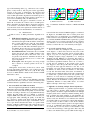
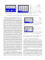
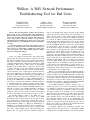
WiSlow: A WiFi Network Performance
Troubleshooting Tool for End Users
Kyung-Hwa Kim
Hyunwoo Nam
Henning Schulzrinne
Columbia University
New York, NY, USA
Email: [email protected]
Columbia University
New York, NY, USA
Email: [email protected]
Columbia University
New York, NY, USA
Email: [email protected]
Abstract—The increasing number of 802.11 APs and wireless
devices results in more contention, which causes unsatisfactory
WiFi network performance. In addition, non-WiFi devices sharing the same spectrum with 802.11 networks such as microwave
ovens, cordless phones, and baby monitors severely interfere
with WiFi networks. Although the problem sources can be easily
removed in many cases, it is difficult for end users to identify the
root cause.
We introduce WiSlow, a software tool that diagnoses the root
causes of poor WiFi performance with user-level network probes
and leverages peer collaboration to identify the location of the
causes. We elaborate on two main methods: packet loss analysis
and 802.11 ACK pattern analysis.
I. I NTRODUCTION
Today, it is common for households to put together home
wireless networks with a private wireless router (access point)
that supports multiple wireless devices. However, the increasing usage of wireless networks inevitably results in more
contention and interference, which causes unsatisfactory WiFi
performance. There are two main sources of performance
degradation. First, WiFi devices connected to the same AP
or nearby APs that use the same channel can cause packet
collisions, i.e., channel contention. Second, non-WiFi devices
such as microwave ovens, cordless phones, and baby monitors
emit severe interference because these devices operate on
the same 2.4 GHz spectrum as 802.11b/g [6]. Although these
problem sources can be easily removed in many cases (e.g., by
relocating the baby monitor, choosing a different channel, or
moving to the 5 GHz band), it is difficult for technically nonsavvy users to even notice the existence of channel contention
or non-WiFi interference. Instead, properly working routers
or service providers are frequently misidentified as the culprit
while the actual root cause remains unidentified. However, isolating the root causes of poor WiFi performance is nontrivial,
even for a network expert, because they show very similar
symptoms at the user level, and special devices are required
in order to investigate the lower layers of the protocol stack.
We introduce WiSlow (“Why is my WiFi slow?”), a
software tool that diagnoses the root causes of poor WiFi
performance with user-level network probes and leverages
peer collaboration to identify their location. We focus on
building software that does not require any additional spectrum
analysis hardware (unlike, e.g., WiSpy [4], AirSleuth [2], or
AirMaestro [1]). In addition, WiSlow does not depend on a
specific network adapter such as the Atheros chipset, which
were used to achieve similar goals in other studies [10], [11].
WiSlow runs on a typical end user’s machine. Currently, it
runs on any machine that supports wireless packet sniffing
enabled by the 802.11 monitor mode. We trace behaviors of
802.11 networks such as retries, Frame Checksum Sequence
(FCS) errors, packet loss, and bit rate adaption, which can
be observed on ordinary operating systems. Our experimental
results show that the statistical patterns of the above variables
vary depending on the problem sources. For example, in the
case of non-WiFi interference, we observed a greater number
of retried packets, fewer FCS errors, and larger variations
in the bit rates compared to channel contention. Correlating
these variables, we can categorize the sources of performance
problems into several distinct groups. In addition, the nonWiFi devices such as baby monitors, cordless phones, and
microwave ovens have different patterns when the number of
UDP packets and 802.11 ACKs are plotted over time. In this
study, we elaborate on two main methods: packet loss analysis
and 802.11 ACK pattern analysis. To improve the accuracy
of the algorithm, WiSlow also uses a heuristic method that
considers the history of interference episodes and matches it
to the common usage characteristics of various devices (e.g.,
microwave ovens are often used intermittently for periods of
5–30 minutes, whereas baby monitors are used continuously)
to ascertain the source of the problem.
Based on our experimental results and heuristic methods,
we have developed an algorithm that successfully distinguishes
channel contention from non-WiFi interference and infers the
product type of the offending device. We believe that this technology will be useful to end users since it can inform them of
what needs to be done in order to improve the performance of
their networks—whether to upgrade their Internet bandwidth
or remove a device that is emitting the interference.
In non-WiFi interference scenarios, another goal is to
identify the location of the source of interference. Although
it is difficult to pinpoint the exact physical location of the
source without the support of hardware or APs, we can infer
the relative location of the problem source by collaborating
with other end users connected to the same wireless network.
WiSlow collects patterns of variables from peers and determines whether others observe the interference at the same
time. If all the machines observe it, it is highly likely that
the problematic source is close to the wireless AP. However,
if only one of the peers observes the interference, the source is
likely to be located close to that peer. Our experimental results
clearly show that this approach is feasible.
In summary, WiSlow uses information obtained from
captured packets and other users to (i) distinguish channel
contention from non-WiFi interference, (ii) infer the product
II. BACKGROUND
Common sources of WiFi performance degradation include:
•
•
•
WiFi channel contention: degradation due to a channel crowded by multiple WiFi devices that compete to
transmit data through an AP. In addition, interference
due to nearby APs that are using the same channel
or adjacent channels cause the similar performance
problems since the APs share the limited capacity of
the channel. We use the term contention in this paper
to refer to this type of performance degradation.
Non-WiFi interference: interference due to non-WiFi
devices that use the same 2.4 GHz spectrum as the
802.11b/g networks such as microwave ovens, cordless phones, baby monitors, and Bluetooth devices. In
this paper, we use the term interference to refer to this
type of degradation.
Weak signal: when the signal is not strong enough
due to distance or obstacles, packets can be lost or
corrupted.
Although the extent varies, all the above sources result
in severe performance degradation—some of them even drop
the TCP/UDP throughput to almost zero [10]. In this study,
we focus on WiFi channel contention and common non-WiFi
interference sources.
III. C HALLENGES
In this section, we describe several difficulties analyzing
wireless networks due to end users’ restricted conditions such
as limited hardware capabilities and lack of monitoring data.
A. Inaccurate RSSI and SINR measurement
Received Signal Strength Indication (RSSI) and Signal-toInterference-plus-Noise Ratio (SINR) are generally considered
to be the key factors that indicate the quality of a wireless link.
However, according to Vlavianos et al. [12], RSSI inaccurately
captures the link quality and it is difficult to accurately
compute SINR with commodity wireless cards, thus they are
not appropriate when estimating the quality of the link. We
also observed a similar result when monitoring RSSI and
SINR values. We placed various types of interference sources
close to the AP and measured the values on a general client
machine1 . In Figure 1a, RSSI values with a baby monitor were
consistently higher than a cordless phone, which should be
1 We used a MacBook Pro 2013 (network card: AirPort Extreme, chipset:
Broadcom BCM43 series) in this measurement
1
1
0.8
0.8
BABY MONITOR
CLEAN
DSSS PHONE
FHSS PHONE
0.6
0.6
CLEAN
0.4
MICROWAVE OVEN
%
BABY MONITOR
%
type of the interfering device (e.g., a microwave oven, cordless
phone, or baby monitor), and (iii) point out the approximate
location of the source of interference. We developed and
evaluated an implementation of WiSlow that diagnoses the
cause of WiFi performance degradation and returns reports to
users such as “It appears that a baby monitor located close to
your router is interfering with your WiFi network.”
The remainder of this paper is structured as follows. In
Section II, we describe the common sources of WiFi performance degradation. In Section III, we discuss the restrictions
of an end user’s environment and how WiSlow attempts to
overcome them. Section IV explains the detailed methods of
WiSlow. Finally, Section VII summarizes our conclusions.
0.4
DSSS PHONE
FHSS PHONE
MICROWAVE OVEN
0.2
0
−60
−55
−50
−45
−40
Values
−35
−30
(a) RSSI measurement
−25
0.2
0
20
25
30
35
40
Values
45
50
55
(b) SINR measurement
Fig. 1: Cumulative distribution functions of RSSI and SINR
values
reversed when the measured UDP throughput is considered.
In, Figure 1b, the SINR values with a cordless phone were
higher than even a no-interference case. Furthermore, these
results varied for each experiment. Based on this observation,
we conclude that RSSI and SINR values captured by a general
wireless cards do not correctly represent the level of interference. Therefore, we do not use these metrics for other purposes
besides as a hint in the case of an extremely weak signal.
B. No specific network adapter or driver
We do not make any assumptions about the specific network adapters or drivers that end users may have. Some
Atheros chipsets, which are widely used in research studies,
support a spectral scan that provides a spectrum analysis
of multiple frequency ranges. Rayanchu et al. developed
Airshark [10] and WiFiNet [11] leveraging this feature to
distinguish non-WiFi interferers using a commodity network
card without specialized hardware. Since our tool aims to
provide the best estimation of the problem source, if the
user happens to have this specific network adapter, WiSlow
can adopt the same approach. However, to the best of our
knowledge, only a few chipsets currently provide this feature.
In addition, we failed to discover references to this feature
for any OS other than Linux. Since there are hundreds of
products that use a different chipset and/or OS, it is impractical
to assume that a general end user has this specific setup.
Therefore, we focus instead on analyzing the quality of a
link using user-controllable protocols such as UDP and 802.11
packets. Because the mechanisms of these protocols are not
significantly different for many WiFi devices, we believe
WiSlow can help a wider range of end users.
C. Difficulties in obtaining multiple channel information
Without special hardware or a particular network adapter,
it is still possible to measure signal strength by monitoring
802.11 packets. In addition, signal information from multiple
frequency bands can be obtained by channel switching. It may
help to identify the signal signature of each interfering device. However, without the specialized functionalities of some
wireless cards, the AP must be reset whenever the channels
are switched. This is not practical for general client machines,
not only because it takes a while to scan all the channels,
but also because the frequencies given for the signal samples
are not at a sufficiently fine-grained resolution. Therefore,
we assume that we can only observe a fixed channel of the
network. The disadvantage of this approach is that it may fail
to detect some interferers that operate within another range of
frequencies. However, it is reasonable for WiSlow to ignore
this case because there is no motivation from an end user’s
perspective to detect these interferers if the interference does
not overlap with his/her WiFi network.
D. Lack of monitoring data
Another restriction in the end-user environment is the lack
of a monitoring history. If we assume that we have been
monitoring the machine up to the moment when a performance
problem happens, the diagnosis will be easier because we can
obtain several important clues such as the average quality of
the network’s usual performance, the time when the problem
started, and whether it has happened in the recent past.
However, although the overhead of network monitoring is not
heavy on modern machines, it is difficult to expect that end
users will continuously run such a tool. The more common
scenario is that a user launches a troubleshooting tool like
WiSlow and requests a diagnostic only after he/she has noticed
a severe performance problem. Therefore, we need to design
the tool assuming little or no previous monitoring data. In the
next section, it is explained how WiSlow estimates the problem
source without knowing the baseline quality of the network.
IV. W I S LOW
In this section, we elaborate on the details of probing
methods for identifying the root causes of network interference. First, to investigate the behavior of WiFi networks in
each problem scenario, we artificially inject problems while
transmitting UDP packets between a client (laptop) and an
AP, capturing every packet on the client. Then, we trace the
transport layer (UDP), the 802.11 MAC layer, and some useraccessible 802.11 PHY layer information to ascertain each
problematic scenario’s interference levels and characteristics.
To capture 802.11 packets, WiSlow leverages the monitor
mode that provides the Radiotap [3] header, a standard for
802.11 frame information. The headers are used to extract
the lower layer information such as FCS errors and bit rates.
Sniffing the wireless packets is supported by most Linux and
all Mac OS X machines without additional driver or kernel
modification. Therefore, if we can successfully characterize
each performance-degrading source by probing the transmitted
packets, the same probes will enable WiSlow to identify
the problem on most platforms. However, it is not always
possible to capture wireless packets on some types of OS, e.g.,
Microsoft Windows [5]. Instead, Windows provides several
APIs that report 802.11 packet statistics to user applications.
Those APIs enable WiSlow to run on Windows because they
provide all the information that WiSlow must extract from the
802.11 packets. In summary, WiSlow can operate properly
if the client’s machine supports wireless packet sniffing or
provides a set of appropriate APIs.
In the following sections, we explain WiSlow’s two main
diagnostic methods, packet loss analysis and ACK pattern
analysis.
A. Packet loss analysis
First, we found that each problem source varies in their
packet loss characteristics, represented by three statistics: 1)
the number of 802.11 retries, 2) the number of FCS errors,
and 3) the bit rates. In each experiment, we measured these
values on a client laptop while downloading 100 MB of packets
from an AP. The values were recorded for each 100 KB of
UDP packets received. Thus, we collected a total of 1,000
samples for each experiment. We repeated this experiment for
different scenarios including channel contention and non-WiFi
interferences. To simulate channel contention, we set up several laptops sending bulk UDP packets to the AP. To generate
non-WiFi interference, we placed each interfering device (baby
monitors, microwave ovens, and cordless phones) close to the
AP (about 20 cm) and measured the effect on the client placed
at various distances from the AP, e.g., 5 m, 10 m, and 20 m. (In
this study, we did not consider the simultaneous interference
of multiple devices.) Note that the client downloaded 100 MB
of UDP packets for each experiment to collect a statistically
meaningful amount of samples, but when actually probing on
an end user’s machine, WiSlow only needs to transmit 10
MBytes of packets to identify the root cause, which takes
reasonable amount of time (20–50 s) for a problem diagnosis
application.
1) Retry and bit rate: Since an 802.11 retry and bit rate
reduction are both initiated by a packet loss, their temporal
changes are closely correlated; when a packet loss occurs, the
bit rate decreases by the 802.11 rate adaption algorithm. The
probability of packet loss then decreases due to the reduced bit
rate, which lowers the number of retries. After that, the bit rate
gradually increases again due to the reduced packet loss, which
leads to a higher probability of packet loss and retries. In other
words, if contention or interference exists, it causes packet
losses, and then the bit rate and number of retried packets
repeatedly fluctuate during the subsequent data transmission.
The more interference, the more the fluctuations are observed.
2) FCS errors: Another variable that we trace is the
number of FCS errors. Intuitively, it can be predicted that nonWiFi interference introduces more FCS errors than channel
contention or a no-interference environment because the packet
corruptions are likely to occur more frequently when a medium
is noisy. However, in our experiment, it turned out that a large
number of FCS errors are not necessarily correlated with severe
interference. On the contrary, we often observed that fewer
FCS errors occur with severe non-WiFi interference (e.g.,
interference of a baby monitor) than with channel contention or
even a no-interference environment (Figure 2a). This paradox
can be explained by the low bit rates in the interference case,
which implies that a smaller number of bits are transmitted in
the same bandwidth. Consequently, the number of FCS errors
alone is not enough to characterize interference sources.
3) Packet loss estimation: As we stated above, although
the number of retries, bit rate, and FCS errors are affected
by the current state of the wireless network, they often show
very different statistics for each experiment set. We conjecture
several reasons; the environment is not exactly the same in
every experiment, the occurrence of packet loss is probabilistic
rather than deterministic, and the individual variables fluctuate
over time, affecting each other and leading to different statistics
for a certain period of time. Therefore, it would be more
reasonable to compare the combinations of these statistics
together instead of investigating each variable individually and
consider the distributions of the samples rather than their
temporal changes. First, since the retries occur when the
packets are lost as well as when FCS errors happen, we can
estimate the amount of actual packet loss by subtracting the
number of FCS errors from the number of retries (Equation 1).
1
80
70
0.8
CONTENTION
60
BABY MONITOR
0.6
FHSS PHONE
LOSS
%
BABY MONITOR
CLEAN
FHSS PHONE
50
MICROWAVE OVEN
0.4
40
30
0.2
20
0
0
5
10
15
20
10
25
EAs
0
(a) The number of FCS errors per 100 KB
10
20
30
40
AVAILABLE BITRATE
50
(a) Bit rates and the estimated packet loss with different interference sources
1
0.8
CLEAN
CONTENTION
FHSS PHONE
BABY MONITOR
%
0.6
0.4
0.2
0
0
10
20
30
40
50
EAs
(b) The number of estimated packet loss
per 100 KB
Fig. 2: The CDFs of the number of FCS errors and packet
loss.
NP acketLoss = NRetries − NF CSerrors
(1)
We found that this estimated number of packet losses
more reliably represents the level of interference than the
individual statistics of retries and FCS errors. In other words,
it showed relatively constant results on multiple experiments,
while the others varied for each experiment. Figure 2b shows
the cumulative distribution function (CDF) of the estimated
number of packet loss, where it can be seen that a baby monitor
(video transmitter) causes the most severe amount of packet
loss while contention and cordless phones cause a relatively
small amount of packet loss. Since baby monitors send video
and audio data at the same time, they use more bandwidth
than cordless phones that send audio only, thus causing more
interference. Channel contention has less packet loss because
of the 802.11 collision-avoidance functions such as random
back-off and RTS/CTS that force each client to occupy the
medium in separate time slots. In this case, the divided time
slots caused the degradation of throughput, rather than noise
from other sources. (The impact of a hidden terminal is not
considered in this section.)
Furthermore, we found that the correlation between bit
rate and the estimated number of packet losses shows clearer
differences among various problem sources. In Figure 3a, the
majority of the samples from clean environment are distributed
in a healthy zone (higher bit rate and low packet loss) while
the samples of baby monitors and microwave ovens are widely
dispersed on the coordinate plane. WiSlow uses the correlation
of these two variables to distinguish the level of interference.
Although the problem sources each have their own distribution patterns on the above scatter plot, an end user
cannot infer a root cause by simply matching the measured
statistics with the results of our experiments. This is because
(b) Bit rates and the estimated packet loss with the
same device, a baby monitor, in different environment
Fig. 3: The distribution of the correlation of bit rates and the
estimated packet loss
the measurement of a wireless network is highly affected by
the client’s own environment such as distance from the AP,
signal power, or fading (multi-path and shadowing). In other
words, even though they have the same type of problem, the
statistics of the measured metrics can vary depending on each
end user’s own situation. Note that this is the reason why
simple measurements such as the higher-layer throughput (e.g.,
TCP or UDP) or number of 802.11 retries are not enough to
identify the level of interference and the type of interferers.
Therefore, to apply our approach to end users, it is important
that the measured statistics are independent of the underlying
environment. We found that even if the underlying environment
changes, the extent of the area, where a set of samples
(correlated packet loss and bit rate) are dispersed, remains
similar if the problem source is the same. Figure 3b shows
that even though the two groups of samples from discrete
environments are distributed on different spots on the plane,
their extent is similar. Thus, we first quantify how widely the
samples are dispersed by calculating the Euclidean distances
between each sample and the mean. Figure 4 compares the
CDFs obtained from two experiments that were conducted
with the same baby monitor in two discrete environments.
The CDFs of packet loss estimation (Figure 4a) and bit rates
(Figure 4b) show different distributions while the CDFs of the
Euclidean distances of the samples to the mean show similar
distribution (Figure 4c).
Therefore, WiSlow can use the above CDFs of the distances
to identify the root causes of network interference. We prepare
these CDFs of each problem source in advance, which are
obtained from our experiments. Then, WiSlow traces the
1
1
0.8
1
0.8
BABY MONITOR Ex1
BABY MONITOR Ex2
0.8
BABY MONITOR Ex1
0.6
0.6
%
%
%
0.6
0.4
0.4
0.4
0.2
0.2
0.2
0
5
10
15
20
EAs
25
30
BABY MONITOR Ex1
BABY MONITOR Ex2
BABY MONITOR Ex2
0
10
35
(a) The estimated number of packet loss
15
20
25
30
35
MBps
(b) Bit rates
40
45
50
55
0
0
5
10
15
20
25
Distance
30
35
40
(c) Distance
Fig. 4: The CDFs obtained from two experiments with the same baby monitor in different environment. 100 MB of UDP packets
were transmitted from the AP and the values were sampled every 100 KB.
1
0.8
Group3
Group1
Group2
%
0.6
0.4
0.2
0
0
2
4
6
8
10 12
Distance
14
16
18
20
Fig. 5: The packet loss analysis groups the problem sources
into three groups: 1) a clean environment, 2) contention and
FHSS cordless phones, and 3) microwave ovens and baby
monitors
wireless packets on an end user’s machine, generates a CDF
of the distances, and compares it to the pre-obtained CDFs of
each problem source. For the convenience of identification, we
group the problem sources into three groups by the shape of the
CDFs: no interferers (group 1), light interferers (group 2), and
heavy interferers (group 3). Each group has its representative
CDFs that are determined by multiple experiments (Figure 5).
In our data sets, group 1 indicates a clean environment, group
2 includes channel contention and FHSS cordless phones, and
group 3 contains microwave ovens and baby monitors. WiSlow
examines which representative CDF is the most similar one
to the user’s CDF. To compare the CDFs, WiSlow uses the
Two-Sample KolmogorovSmirnov test (K-S test), a widely
used statistical method that tests whether the two empirical
CDFs obtained from separate experiments have the same
distribution [9]. If the p-value of this test is close to 1, the two
CDFs are likely to come from the same distribution, however,
if the p-value is close to 0, they are likely to come from
different distributions. Since the K-S test not only considers
the average and variance of the samples but also takes into
account the shape of the CDFs, it best fits the purpose of
WiSlow where it is used to pick the most similar distribution
from multiple data sets.
B. ACK Pattern Analysis
The first method is able to determine which type of loss
pattern a problem source has. However, because multiple
problem sources are categorized into each group, we need
another method that further narrows down the root causes.
In this section, we explain the second method, designed to
distinguish several detailed characteristics of non-WiFi devices
such as frequency hopping and duty cycle.
1) Probing method: WiSlow sends bulk UDP packets to
the AP and counts the received 802.11 ACKs to check the
quality of a wireless link within a given period. In order to
detect patterns on the scale of milliseconds, we use a very
small size of UDP packets (12 bytes) that reduces potential
delays such as propagation and processing delays, and we
transmit as many UDP packets as possible to reduce the
intervals between samples. As a result, we received 0–7 ACKs
per millisecond with an average number of 2.7 in a clean
environment.
In the following sections, we describe the results of the
above method when performed with various non-WiFi interferers, and we explain how WiSlow identifies the devices based
on the results.
2) Duty cycle (microwave ovens): Microwave ovens generate severe interference in almost every channel of the 2.4 GHz
band. We identify this heavy interferer using its duty cycle,
which is the ratio of the active duration to the pulse period. It
is known that the duty cycle of microwave ovens is fixed at 0.5
and the dwell time is 16.6 ms (60 Hz) 2 [7]. This implies that
it stays in the ON mode (producing microwaves) for the first
8.3 ms and the OFF mode for the next 8.3 ms. This feature
can be observed by various means such as using a spectrum
analyzer [4] or by signal measurement [10].
Our hypothesis was that a user-level probe could also detect
this on-off pattern if the network packets were monitored on a
millisecond timescale because the packets would be lost only
when the interferer was active (on mode). To validate this
assumption, we implemented the above method and plotted the
number of successfully received 802.11 ACKs per millisecond.
As a result, a clearly perceptible waveform with a 0.5 duty
cycle is observed in Figure 6a; the number of ACKs is over
five for the first 8 ms and zero during the next 8 ms. This
pattern repeats while the microwave oven is running. This
result becomes clearer when it is converted to the frequency
domain (Figure 6b). The highest peak is at 60 Hz, which means
the exact cycle is 16.6 ms. This number is exactly the same
as the known duty cycle of microwave ovens.
Consequently, if a perceptible cycle is detected from this
probing method and the period matches a well-known value,
WiSlow determines that the current interference is due to a
2 This frequency could be 50 Hz in other countries (e.g., Europe and most
of Asia) where 50 Hz AC power is used.
6
10
5
8
4
Magnitude
EAs
4
12
6
4
2
0
1.45
x 10
3
2
1
1.455
1.46
1.465
Time
1.47
1.475
1.48
4
x 10
(a) Time domain (Microwave oven)
0
0
100
200
300
Frequency
400
500
(b) Frequency domain (Microwave oven)
(c) Time domain (Microwave oven) - top 10
frequencies
Fig. 6: The number of 802.11 ACKs per 100 KB of UDP packets with interference of a microwave oven
4
6
x 10
Magnitude
5
4
3
2
1
0
0
100
200
300
Frequency
400
500
(a) A baby monitor: frequency (b) A baby monitor: time domain
domain
- top 10 frequencies
4
6
x 10
ude
t
Magni
5
Magnitude
particular type of device (e.g., 60 Hz for microwave ovens).
3) Frequency hopping (baby monitors): The duty cycle of
typical video transmitters such as wireless camera is known as
one [10]. It means that they send and receive data constantly,
implying that they continuously interfere with WiFi networks
without any off period. Baby monitors, which transmit video
and audio data constantly, also have a similar characteristic.
Therefore, intuitively, we do not expect to observe similar ACK
patterns as those observed in the microwave oven experiment.
However, when converting the plot from the time domain to
the frequency domain, we observe another notable pattern.
Figure 7a shows that there are multiple high peaks set apart by
a specific interval, i.e., 43 Hz (occurring at 43, 86, 129, and 172
Hz). This is in contrast to the microwave ovens that showed
only one significantly high peak at 60 Hz (Figure 6b). We
conjecture that these peaks are caused by frequency hopping;
a frequency hopper switches its frequency periodically, and
interference occurs when it hops to a nearby frequency of the
current WiFi channel. However, the frequency-hopping device
does not necessarily return to the same frequency at a regular
period because the frequency of the next hop is randomly
chosen. This randomness instead creates diverse cycles with
different periods. However, these periods are multiples of a
specific number due to the fixed hopping interval. For clarity,
we plot a quantized time-domain graph (Figure 7b) that is
converted back from the frequency-domain graph. We used
the 10 highest frequencies from Figure 7a. In the time-domain
graph, the number of ACKs (y-axis) fluctuates periodically,
however, note that the heights of the peaks vary. The possible
explanation is as follows: the number of ACKs is large when
the device hops far from the current WiFi channel and is
relatively small when it hops to a nearby frequency. If the
device hops into the exact range of the WiFi channel, the
number of 802.11 ACKs drops almost to zero. In other words,
there are multiple levels of interference, which depend on how
closely in frequency the device hops to the frequency used by
the WiFi channel. These multiple levels of interference create
several pulses that have different magnitudes and frequencies.
Finally, because the hopping interval is fixed, the frequencies
of the created pulses are synchronized such that the periods of
the cycles are multiples of a specific value.
Consequently, we can distinguish frequency-hopping devices by determining whether the number of 802.11 ACKs has
multiple high peaks with a certain interval in the frequency
domain. We check this by linear regression of the peak
frequencies; if the correlation coefficient is greater than 0.9,
4
3
2
1
0
0
100
200
300
Frequency
400
500
(c) A cordless phone: frequency (d) A cordless phone: time dodomain
main - top 10 frequencies
Fig. 7: The number of 802.11 ACKs per 100 KB of UDP
packets with a baby monitor and a cordless phone
we consider it to be a frequency-hopping device.
However, it is obvious that we cannot conclude that every
frequency-hopping device is a specific type of device such as
a baby monitor. Therefore, WiSlow needs to take into account
the results of both the first method and this second method
to identify the problem source precisely. For example, if a
problem source is classified as group 3 (by the first method)
and a frequency hopper (by the second method), we consider
it to be a baby monitor. Of course, it is still possible that
another type of device not discussed in this study has the
same characteristics as a baby monitor. We discuss this case
in Section ??.
4) Fixed frequency (analog cordless phones): Typical
analog cordless phones use a fixed frequency, so they usually
interfere only with a small number of channels. (The analog
phones we tested only interfered with Channel 1.) Because
they do not change frequency, severe interference occurs if
the current WiFi channel overlaps with the frequency of the
phone. In addition, their duty cycle is usually one, which
implies that no ACK cycle exists. In our experiments, the
Interference
Source
No Interference
Loss Type = B
Packet Analysis
Loss Type = A
Contention
Clean
A
WiFi
Interference
Probe 1
B
Non-WiFi
Interference
Audio (Voice)
Loss Type = B,
ACK Cycle = hopping
Probe 3
Frequency
Hopping
Fixed
Frequency
Fixed ACK cycle
(duty cycle = a, a<1)
Video
+ Audio (Voice)
Loss Type = C,
ACK Cycle = hopping
Probe 2
Fig. 9: Probing for localizing an interference source
No ACK cycle
(duty cycle = 1)
Fig. 8: The classification of problem sources by WiSlow’s
methods
UDP throughput stayed very low and no explicit ACK cycle
(no hopping) was observed, as expected. Therefore, WiSlow
determines an analog cordless phone as the interferer if there
is severe UDP throughput degradation but no explicit ACK
cycle or duty cycle is detected. However, this could be true of
other fixed frequency devices such as wireless video cameras
that are not discussed in this paper. Currently, when WiSlow
detects this type of device, it informs the user that a fixed
frequency device has been detected, and suggests that several
devices could be the cause, such as analog cordless phones
and wireless video cameras.
5) Mixed (hopping and duty cycle): A Frequency Hopping
Spread Spectrum (FHSS) phone is another example of a device
that explicitly shows the hopping patterns that we described
above. In addition, it is known that some FHSS phones have
a specific pulse interval, which was verified by Rayanchu
et al. [10] using signal measurement. We also confirmed
this feature with our user-level probes. Figure 7c shows the
frequency domain of 802.11 ACKs. It shows similar patterns
as the microwave ovens (low duty cycle devices) rather than
the baby monitors (frequency-hopping devices) even though
it also uses frequency hopping. This is because the duty
cycle influences the shape of the waveform more than the
hopping effect. Therefore, it is possible to use this duty cycle
to distinguish the FHSS cordless phones as we did for the
microwave ovens. In this case, we use the frequencies, 100 and
200 Hz, to determine the FHSS cordless phone interference.
However, to the best of our knowledge, there is no standard
regarding the period of the duty cycle for FHSS cordless
phones. This means it can vary depending on the product.
Therefore, if a duty cycle is detected but the period is an
unknown value, WiSlow fails to identify the exact product
type. In this case, we provide our best estimate of the problem
source by listing a possible set of candidates.
V. L OCATING I NTERFERING D EVICES
Once WiSlow detects non-WiFi interference and identifies
the type of device causing it, the next step is to locate its
physical location. Device localization has been investigated
intensively in many research fields. A number of research
studies on indoor location tracking have tried to pinpoint the
location of client laptops or smartphones using various meth-
ods cite. WiFiNet [11] pinpoints the location of the interference
source using multiple APs that use Airshark [10]. Although we
leverage a similar cooperative diagnosis approach, we focus
on the collaboration of multiple end users instead of APs.
However, it is not easy to pinpoint the exact physical location
of the source by end users because they cannot obtain precise
signal information. Instead, we attempt to infer the relative
location of the problem source. The basic mechanism is that
an end user (probing client) first requests multiple cooperative
clients to perform WiSlow diagnostics as described in previous
sections. Then it checks whether the other client machines
observe the same interference as itself. If all the cooperative
client machines observe a particular type of interference at the
same time, it is likely that the problematic source is close to
the AP because this would affect the entire wireless network.
However, if only one of the clients observes the interference,
the source is highly likely to be located close to that client.
A. Cooperative Probing
Figure 9 illustrates the details of the cooperative probing
approach. We assume that the clients already have WiSlow
installed and have contact information of the others, i.e., IP
address and port number. Each probing process takes about
30-40 s; thus, it took a few minutes to collect the results from
the three clients in our experiment. Then, WiSlow checks
whether the other clients have also detected the same type
of interference.
VI. R ELATED W ORK
Airshark [10] uses a commodity WiFi network adapter
to identify interference sources. It leverages a spectral scan
to obtain signal information from multiple frequency ranges.
It identifies the interference sources very accurately (over
95%) by analyzing the spectrum data using various methods.
However, it is not easy to apply this approach for typical end
users because collecting high-resolution signal samples across
the spectrum is impossible if the network card does not support
this functionality.
WiFiNet [11] identifies the impact of non-WiFi interference
and finds its location using observations from multiple APs that
are running Airshark. Although the authors briefly mention
that WiFiNet could be used by end users, they focus more on
building infrastructure using APs, while WiSlow focuses on
end users and their cooperation to identify the location of the
interference source.
Kanuparthy et al. [8] proposed an approach similar to
WiSlow in terms of using user-level information to identify
interference sources. They distinguished congestion (channel
contention) by measuring the one-way delay of different sizes
of packets. Then, they investigated the delay patterns to distinguish a hidden terminal from a weak signal. While this study
focused on congestion, weak signals, and hidden terminals,
WiSlow focuses on not only congestion and signals but also
the detailed identification of non-WiFi interference sources.
VII. C ONCLUSION
We designed WiSlow, a WiFi performance trouble shooting
application, specialized to detect non-WiFi interferences. WiSlow distinguishes 802.11 channel contention from non-WiFi
interference and identifies the type of interfering devices. We
introduced two main methods: packet loss analysis and 802.11
ACK pattern analysis. These methods uses user-accessible
packet trace information such as UDP and 802.11 ACKs.
In addition, WiSlow leverages peer collaboration to identify
the physical location of the sources of WiFi performance
degradation.
[1]
[2]
[3]
[4]
[5]
[6]
[7]
[8]
[9]
[10]
[11]
[12]
R EFERENCES
AirMaestro. http://www.bandspeed.com/products/products.php. [Online; accessed May 2013].
AirSleuth. http://nutsaboutnets.com/airsleuth-spectrum-analyzer/. [Online; accessed May 2013].
Radiotap. http://www.radiotap.org/. [Online; accessed May 2013].
Wi-Spy. http://www.metageek.net/. [Online; accessed May 2013].
WLAN packet capture. http://wiki.wireshark.org/CaptureSetup/WLAN.
[Online; accessed May 2013].
S. Gollakota, F. Adib, D. Katabi, and S. Seshan. Clearing the RF smog:
making 802.11n robust to cross-technology interference. In Proc. of
ACM SIGCOMM’11, Toronto, Ontario, Canada, Aug. 2011.
A. Kamerman and N. Erkocevic. Microwave oven interference on
wireless lans operating in the 2.4 GHz ISM band. In Proc. of PIMRC
’97, Helsinki, Finland, Sep. 1997.
P. Kanuparthy, C. Dovrolis, K. Papagiannaki, S. Seshan, and
P. Steenkiste. Can user-level probing detect and diagnose common
home-WLAN pathologies. Computer Communication Review, 42(1):7–
15, 2012.
F. J. Massey Jr. The Kolmogorov-Smirnov test for goodness of fit.
Journal of the American statistical Association, 46(253):68–78, 1951.
S. Rayanchu, A. Patro, and S. Banerjee. Airshark: Detecting non-WiFi
RF devices using commodity WiFi hardware. In Proc. of ACM IMC
’11, Berlin, Germany, Nov. 2011.
S. Rayanchu, A. Patro, and S. Banerjee. Catching whales and minnows using WiFiNet: Deconstructing non-WiFi interference using WiFi
hardware. In Proc. of USENIX NSDI’12, San Jose, CA, USA, Apr.
2012.
A. Vlavianos, L. K. Law, I. Broustis, S. V. Krishnamurthy, and
M. Faloutsos. Assessing link quality in IEEE 802.11 wireless networks:
Which is the right metric? In Proc. of PIMRC’08, Cannes, France, Sep.
2008.