Download BDSIM User's Manual v0.6

BDSIM User’s Manual v0.6
I. Agapov, S. T. Boogert, L. C. Deacon,
S. Malton, L. Nevay, J.Snuverink
revision 0.6, last updated 22 May 2015
i
Table of Contents
BDSIM v0.6 User’s Manual . . . . . . . . . . . . . . . . . . . . . . . 1
1
About BDSIM . . . . . . . . . . . . . . . . . . . . . . . . . . . . . . . . . . 1
2
Obtaining, Installing and Running . . . . . . . . . . . . 1
3
Lattice description . . . . . . . . . . . . . . . . . . . . . . . . . . . . . . 2
3.1
3.2
3.3
Program structure . . . . . . . . . . . . . . . . . . . . . . . . . . . . . . . . . . . . . . . . . . . . . 3
Arithmetical expressions . . . . . . . . . . . . . . . . . . . . . . . . . . . . . . . . . . . . . . . 3
Physical elements and Entities. . . . . . . . . . . . . . . . . . . . . . . . . . . . . . . . . . 4
3.3.1 Coordinate system . . . . . . . . . . . . . . . . . . . . . . . . . . . . . . . . . . . . . . . . 6
3.3.2 Units. . . . . . . . . . . . . . . . . . . . . . . . . . . . . . . . . . . . . . . . . . . . . . . . . . . . . . 6
3.3.3 marker . . . . . . . . . . . . . . . . . . . . . . . . . . . . . . . . . . . . . . . . . . . . . . . . . . . . 7
3.3.4 drift . . . . . . . . . . . . . . . . . . . . . . . . . . . . . . . . . . . . . . . . . . . . . . . . . . . . . 7
3.3.5 rbend . . . . . . . . . . . . . . . . . . . . . . . . . . . . . . . . . . . . . . . . . . . . . . . . . . . . . 7
3.3.6 sbend . . . . . . . . . . . . . . . . . . . . . . . . . . . . . . . . . . . . . . . . . . . . . . . . . . . . . 8
3.3.7 quadrupole . . . . . . . . . . . . . . . . . . . . . . . . . . . . . . . . . . . . . . . . . . . . . . . 8
3.3.8 sextupole . . . . . . . . . . . . . . . . . . . . . . . . . . . . . . . . . . . . . . . . . . . . . . . . 9
3.3.9 octupole . . . . . . . . . . . . . . . . . . . . . . . . . . . . . . . . . . . . . . . . . . . . . . . . . 9
3.3.10 multipole . . . . . . . . . . . . . . . . . . . . . . . . . . . . . . . . . . . . . . . . . . . . . . . 9
3.3.11 rf . . . . . . . . . . . . . . . . . . . . . . . . . . . . . . . . . . . . . . . . . . . . . . . . . . . . . . 10
3.3.12 rcol . . . . . . . . . . . . . . . . . . . . . . . . . . . . . . . . . . . . . . . . . . . . . . . . . . . . 10
3.3.13 ecol . . . . . . . . . . . . . . . . . . . . . . . . . . . . . . . . . . . . . . . . . . . . . . . . . . . . 11
3.3.14 muspoiler . . . . . . . . . . . . . . . . . . . . . . . . . . . . . . . . . . . . . . . . . . . . . . 11
3.3.15 solenoid . . . . . . . . . . . . . . . . . . . . . . . . . . . . . . . . . . . . . . . . . . . . . . . 11
3.3.16 hkick and vkick . . . . . . . . . . . . . . . . . . . . . . . . . . . . . . . . . . . . . . . . 12
3.3.17 transform3d . . . . . . . . . . . . . . . . . . . . . . . . . . . . . . . . . . . . . . . . . . . . 12
3.3.18 element . . . . . . . . . . . . . . . . . . . . . . . . . . . . . . . . . . . . . . . . . . . . . . . . 12
3.3.19 line . . . . . . . . . . . . . . . . . . . . . . . . . . . . . . . . . . . . . . . . . . . . . . . . . . . . 13
3.3.20 matdef . . . . . . . . . . . . . . . . . . . . . . . . . . . . . . . . . . . . . . . . . . . . . . . . . 13
3.3.21 laser . . . . . . . . . . . . . . . . . . . . . . . . . . . . . . . . . . . . . . . . . . . . . . . . . . . 15
3.3.22 gas . . . . . . . . . . . . . . . . . . . . . . . . . . . . . . . . . . . . . . . . . . . . . . . . . . . . . 15
3.3.23 spec keyword . . . . . . . . . . . . . . . . . . . . . . . . . . . . . . . . . . . . . . . . . . . 15
3.3.24 Element number . . . . . . . . . . . . . . . . . . . . . . . . . . . . . . . . . . . . . . . . 15
3.3.25 Element attributes . . . . . . . . . . . . . . . . . . . . . . . . . . . . . . . . . . . . . . 16
3.3.26 Editing apertures . . . . . . . . . . . . . . . . . . . . . . . . . . . . . . . . . . . . . . . 16
3.3.27 Material table . . . . . . . . . . . . . . . . . . . . . . . . . . . . . . . . . . . . . . . . . . . 16
3.4 Run control and output . . . . . . . . . . . . . . . . . . . . . . . . . . . . . . . . . . . . . . . 16
3.4.1 option . . . . . . . . . . . . . . . . . . . . . . . . . . . . . . . . . . . . . . . . . . . . . . . . . . . 17
3.4.2 beam . . . . . . . . . . . . . . . . . . . . . . . . . . . . . . . . . . . . . . . . . . . . . . . . . . . . . 19
3.4.3 sample and csample . . . . . . . . . . . . . . . . . . . . . . . . . . . . . . . . . . . . . 22
3.4.4 dump . . . . . . . . . . . . . . . . . . . . . . . . . . . . . . . . . . . . . . . . . . . . . . . . . . . . . 23
ii
3.4.5 use . . . . . . . . . . . . . . . . . . . . . . . . . . . . . . . . . . . . . . . . . . . . . . . . . . . . . . 23
3.4.6 print . . . . . . . . . . . . . . . . . . . . . . . . . . . . . . . . . . . . . . . . . . . . . . . . . . . . 23
4
Visualization . . . . . . . . . . . . . . . . . . . . . . . . . . . . . . . . . . . 24
5
Physics . . . . . . . . . . . . . . . . . . . . . . . . . . . . . . . . . . . . . . . . . 25
5.1
5.2
5.3
6
physicsList option . . . . . . . . . . . . . . . . . . . . . . . . . . . . . . . . . . . . . . . . . . . . . 25
Transportation . . . . . . . . . . . . . . . . . . . . . . . . . . . . . . . . . . . . . . . . . . . . . . . . 26
Tracking accuracy . . . . . . . . . . . . . . . . . . . . . . . . . . . . . . . . . . . . . . . . . . . . . 26
Output Analysis . . . . . . . . . . . . . . . . . . . . . . . . . . . . . . . 26
Appendix A
Geometry description formats . . . 27
A.1 gmad format . . . . . . . . . . . . . . . . . . . . . . . . . . . . . . . . . . . . . . . . . . . . . . . . . .
A.2 mokka . . . . . . . . . . . . . . . . . . . . . . . . . . . . . . . . . . . . . . . . . . . . . . . . . . . . . . . .
A.2.1 Describing the geometry . . . . . . . . . . . . . . . . . . . . . . . . . . . . . . . . .
A.2.1.1 Common Table Parameters . . . . . . . . . . . . . . . . . . . . . . . . .
A.2.1.2 ’Box’ Solid Types . . . . . . . . . . . . . . . . . . . . . . . . . . . . . . . . . . .
A.2.1.3 ’Trapezoid’ Solid Types . . . . . . . . . . . . . . . . . . . . . . . . . . . . .
A.2.1.4 ’Cone’ Solid Types . . . . . . . . . . . . . . . . . . . . . . . . . . . . . . . . . .
A.2.1.5 ’Torus’ Solid Types . . . . . . . . . . . . . . . . . . . . . . . . . . . . . . . . .
A.2.1.6 ’Polycone’ Solid Types . . . . . . . . . . . . . . . . . . . . . . . . . . . . . .
A.2.1.7 ’Elliptical Cone’ Solid Types . . . . . . . . . . . . . . . . . . . . . . . .
A.2.2 Creating a geometry list . . . . . . . . . . . . . . . . . . . . . . . . . . . . . . . . .
A.2.3 Defining a Mokka element in the GMAD file . . . . . . . . . . . . .
A.3 gdml . . . . . . . . . . . . . . . . . . . . . . . . . . . . . . . . . . . . . . . . . . . . . . . . . . . . . . . . .
27
28
28
29
32
32
33
33
34
35
35
36
36
Appendix B
Field description formats . . . . . . . . 36
Appendix C
Bunch description formats . . . . . . . 36
Appendix D
Known Issues . . . . . . . . . . . . . . . . . . . . . 37
References . . . . . . . . . . . . . . . . . . . . . . . . . . . . . . . . . . . . . . . . . 37
Chapter 2: Obtaining, Installing and Running
1
BDSIM v0.6 User’s Manual
This file is updated automatically from manual.texi, last updated on 22 May 2015.
1 About BDSIM
BDSIM is a Geant4 [1] extension toolkit for simulation of particle transport in accelerator
beamlines. It provides a collection of classes representing typical accelerator components,
a collection of physics processes for fast tracking, procedures of “on the fly” geometry
construction and interfacing to ROOT analysis [2].
2 Obtaining, Installing and Running
BDSIM can be downloaded from
https://twiki.ph.rhul.ac.uk/twiki/bin/view/PP/JAI/BdSim. This site also contains
information on documentation, projects and installation. Alternatively, a development
version is from the Git repository, instructions are at https://twiki.ph.rhul.ac.uk/
twiki/bin/view/PP/JAI/BDsimInstall.
Download the tarball and extract the source code. Make sure Geant4 is installed and
appropriate environment variables defined. Then go through the configuration procedure
by running the ./configure script.
./configure
It will create a Makefile from template defined in Makefile.in. You may want to edit
the Makefile manually to meet your needs (if your CLHEP version is greater than 2.x put
-DCLHEP VERSION=9). Then start the compilation by typing
make
If the compilation is successful the bdsim executable should be created in $(BDSIM)/bin/$(ARCH) where $(BDSIM) is the directory specified during configuration, and
$(ARCH) is of the form $(OSTYPE)-$(COMPILER), eg Linux-g++. Next, set up the
(DY)LD LIBRARY PATH variable to point to the ./parser directory, and also to the
directory where libbdsim.so is if building shared libraries.
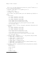
BDSIM is invoked by the command bdsim options
where the options are
--file=<filename>
: specify the lattice file
--output=<fmt>
: output format (root|ascii), default ascii
--outfile=<file>
: output file name. Will be appended with _N
where N = 0, 1, 2, 3... etc.
--vis_mac=<file>
: visualization macro script, default vis.mac
--gflash=N
: whether or not to turn on gFlash fast shower parameterisation.
--gflashemax=N
: maximum energy for gflash shower parameterisation in GeV. Defau
--gflashemin=N
: minimum energy for gflash shower parameterisation in GeV. Defau
--help
: display this message
--verbose
: display general parameters before run
--verbose_event
: display information for every event
Chapter 3: Lattice description
2
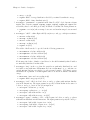
--verbose_step
--verbose_event_num=N
--batch
--outline=<file>
--outline_type=<fmt>
:
:
:
:
:
--materials
--circular
--seed=N
--seedstate=<file>
:
:
:
:
display tracking information after each step
display tracking information for event number N
batch mode - no graphics
print geometry/optics info to <file>
type of outline format
where fmt = optics | survey
list materials included in BDSIM by default
assume circular machine - turn control
the seed to use for the random number generator
file containing CLHEP::Random seed state - overrides other seed
To run BDSIM one first has to define the beamline geometry in a file which is then
passes to BDSIM via the --file command line option, for example
bdsim --file=line.gmad --output=root --batch
The next section describes how to do it in more detail.
3 Lattice description
The beamline, beam properties and physics processes are specified in the input file written
in the GMAD language which is a variation of MAD-X language extended to handle sophisticated geometry and parameters relevant to radiation transport. GMAD is described in
this section. Examples of input files can be found in the BDSIM distribution in the examples
directory. In order to convert a MAD file into a GMAD one, a utility called mad2gmad.sh
is provided in the utils directory.
The following MAD commands are not supported:
• assign
• bmpm
• btrns
• envelope
• optics1
• title
• option
• plot
• print
• return
• survey2
• title
The following MAD commands:
1
2
To dump the optical properties of the lattice one can invoke bdsim with the --outline=file.txt
--outline_type=optics options.
To compute the coordinates of all machine elements in a global reference system one can invoke bdsim
with the --outline=file.txt --outline_type=survey options
Chapter 3: Lattice description
•
•
•
•
3
moni
monitor
wire
prof
are replaced with the marker command.
3.1 Program structure
A GMAD program consists of a sequence of element definitions and control commands. For
example, tracking a 1 GeV electron beam through a FODO cell will require a file like this:
mk: marker;
qf: quadrupole, l=0.5*m, k1=0.1*m^-2;
qd: quadrupole, l=0.5*m, k1=-0.1*m^-2;
d: drift, l=0.5*m;
fodo : line=(qf,d,qd,d,mk);
use, period=fodo;
beam, particle="e-",energy=1*GeV;
option, beampipeRadius=5*cm, beampipeThickness=5*mm;
sample, range=mk;
Generally, the user has to define a sequence of elements (with drift, quadrupole, line
etc.), then select the beamline with the use command and specify beam parameters and
other options with beam and option commands. The sample and csample commands
control what sort of information will be recorded during the execution.
The parser is case sensitive. However, for convenience of porting lattice descriptions from
MAD the keywords can be both lower and upper case. The GMAD language is discussed
in more detail in this section.
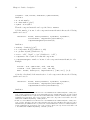
3.2 Arithmetical expressions
Throughout the program a standard set of arithmetical expressions is available. Every
expression is ended with a semicolon, for example:
x=1;
y=2.5-x;
z=sin(x) + log(y) - 8e5;
Available
Available
Available
Available
• sqrt
3
binary operators are: +, -, *, /, ^
unary operators are: +, Boolean operators are: <, >, <=, >=, <>, ==
functions3 are:
see add func(..) in parser/gmad.cc
Chapter 3: Lattice description
•
•
•
•
•
•
•
•
•
4
cos
sin
exp
log
tan
asin
acos
atan
abs
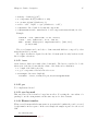
3.3 Physical elements and Entities
GMAD implements almost all the standard MAD elements, but also allows to define arbitrary geometric entities and magnetic field configurations. The geometry description
capabilities are extended by using “drivers” to other geometry description formats, which
makes interfacing and standardisation easier. The syntax of a physical element declaration
is
element_name : element_type, attributes;
for example
qd : quadrupole, l = 0.1*m, k1 = 0.01;
element_type can be of basic type or inherited. Allowed basic types are
• marker
• drift
• rbend
• sbend
• quadrupole
• sextupole
• octupole
• multipole
• vkick
• hkick
• rf
• rcol
• ecol
• solenoid
• laser
• transform3d
• element
All elements except marker, element, ecol, transform3d and rcol are modelled with a
beampipe and an outer surrounding volume. The beampipe form, dimensions and materials
are controlled by the following parameters:
Chapter 3: Lattice description
5
• beampipeRadius
• beampipeThickness
• beampipeMaterial
• apertureType
• aper1
• aper2
• aper3
• aper4
• vacuumMaterial
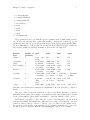
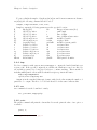
These parameters can be set with the option command as the default parameters and
also on a per element basis, that overrides the defaults for that specific element. Up to four
parameters can be used to specify the aperture shape (aper1, aper2, aper3, aper4). These
are used differently for each aperture model and match the MADX aperture definitions.
The required parameters and their meaning are given in the following table.
Aperture
Type
circular
Number of
parameters
1
rectangular
2
ellipse
2
lhcscreensimple 3
lhcscreen
3
rectellipse
4
racetrack
3
octagon
4
aper1
aper2
aper3
aper4
beam pipe
radius
x half width
x semi-axis
x half width
of rectangle
x half width
of rectangle
x half width
of rectangle
horizontal
offset
of
circle
x half width
NA
NA
NA
y half width
y semi-axis
y half width
of rectangle
y half width
of rectangle
y half width
of rectangle
vertical offset of circle
NA
NA
radius
of
circle
radius
of
circle
x semi-axis
of ellipse
radius of circular part
NA
NA
NA
y half width
angle 1 [rad]
angle 2 [rad]
NA
y semi-axis
of ellipse
NA
Currently, only circular and rectangular are implemented. More models will be completed
shortly.
The outer volume is represented (with the exception of the drift element) by a cylinder
with inner radius equal to the beampipe outer radius and with outer radius given by default
by the global boxSize option, which can usually be overridden with the “outR” option.
In Geant4 it is possible to drive different “regions” each with their own production
cuts and user limits. In BDSIM three different regions exist, each with their own user
defined production cuts (see Chapter 5 [Physics], page 25). These are the default region,
the precision region and the approximation region. Beamline elements can be set to the
precision region by setting the attribute precisionRegion equal to 1. For example:
Chapter 3: Lattice description
6
d1: drift, l=1*m, precisionRegion=1;
creates a drift element in the precision region. Elements in the precision region also
retain detailed information about energy deposition (every individual hit is stored rather
than binned into a histogram).
The third and final region is the “approximation region”. Volumes within the “mokka”
defined elements can be assigned to this region (see Appendix A [Geometry], page 27).
An already defined element can be used as a new element type. The child element will
have the attributes of the parent.
q:quadrupole, l=1*m, k1=0.1;
qq:q,k1=0.2;
3.3.1 Coordinate system
The usual accelerator coordinate system is assumed, see [3].
3.3.2 Units
In GMAD the SI units are used.
length
[m] (metres)
time
[s] (seconds)
angle
[rad] (radians)
quadrupole coefficient
[m−2 ]
multipole coefficient 2n poles
[m−n ]
electric voltage
[MV] (Megavolts)
electric field strength
[MV/m]
particle energy
[GeV]
particle mass
[GeV/c2 ]
particle momentum
[GeV/c]
beam current
[A] (Amperes)
particle charge
[e] (elementary charges)
emittances
[pi m mrad]
density
[g/cm3 ]
temperature
[K] (Kelvin)
pressure
[atm] (atmosphere)
mass number
[g/mol]
There are some predefined numerical values4 are:
pi
3.14159265358979
GeV
1
m
1
−9
eV
10
cm
10−2
−6
keV
10
mm
10−3
−3
MeV
10
um
10−6
4
see add var(..) in parser/gmad.cc
Chapter 3: Lattice description
7
TeV
103
nm
10−9
MV
1
s
1
Tesla
1
ms
10−3
rad
1
us
10−6
mrad
10−3
ns
10−9
8
clight
2.99792458 ∗ 10
for example, one can write either 100*eV or 0.1*keV when energy constants are concerned.
3.3.3 marker
marker has no effect (no volume is associated to it) but allows one to identify a position in
the beam line (say, where a sampler will be placed). It has no attributes.
Example:
m1 : marker;
3.3.4 drift
drift defines a straight section of beampipe with no magnetic field. Its volume contains
only the vacuum beampipe (no outer iron cylinder).
Attributes:
• l - length [m] (default 0)
• aper1 - aper1 [m]
• aper2 - aper2 [m]
• aper3 - aper3 [m]
• aper4 - aper4 [m]
• beampipeMaterial - material the beampipe is made of (default “StainlessSteel”)
• vacuumMaterial - material used for the vacuum - for example a user defined material
defined before this item
Example:
d13 : drift, l=0.5*m;
3.3.5 rbend
rbend defines a rectangular bending magnet. Attributes:
• l - length [m] (default 0)
• angle - bending angle [rad] (default 0)
• B - magnetic field [T]
• material - the magnet material (default set to “Iron”)
• k1 - normal quadrupole coefficient k1 = 1/(Bρ) dBy /dx [m−2 ] Positive k1 means horizontal focusing of positively charged particles (default 0).
Chapter 3: Lattice description
8
• boxSize - the full width of the magnet outer volume [m]
• additionally, all of the drift parameters
when B is set, this defines a magnet with appropriate field strength and angle is not
taken into account. Otherwise, the value of B that corresponds to bending angle angle for
a particle with the momentum of the design energy of the model (as specified by energy
by the beam command), is calculated and used in the simulations.
Example :
rb1 : rbend, l=0.5*m, angle = 0.01;
3.3.6 sbend
sbend defines a sector bending magnet. Attributes:
• l - length [m] (default 0)
• angle - bending angle [rad] (default 0)
• B - magnetic field [T]
• material - the magnet material (default set to “Iron”) k1 = 1/(Bρ) dBy /dx [m−2 ]
Positive k1 means horizontal focusing of positively charged particles (default 0).
• boxSize - the full width of the magnet outer volume [m]
• additionally, all of the drift parameters
The meaning of B and angle is the same as for rbend.
Example :
sb1 : sbend, l=0.5*m, angle = 0.01;
3.3.7 quadrupole
quadrupole defines a quadrupole. Attributes:
• l - length [m] (default 0)
• k1 - normal quadrupole coefficient k1 = 1/(Bρ) dBy /dx [m−2 ] Positive k1 means horizontal focusing of positively charged particles (default 0). dBy /dx is the magnetic field
gradient, while (Bρ) is the magnetic “rigidity”: Bρ (T*m) = p(GeV)/(0.299792458 *
|charge(e)|)
• ks1 - skew quadrupole coefficient ks1 = 1/(Bρ) dBy /dx [m−2 ] where (x,y) is now a coordinate system rotated by 45 degrees around s with respect to the normal one.(default
0).
• tilt - roll angle [rad] about the longitudinal axis, clockwise.
• material - the magnet material (default set to “Iron”)
• boxSize - the full width of the magnet outer volume [m]
• additionally, all of the drift parameters
Example :
Chapter 3: Lattice description
9
qf : quadrupole, l=0.5*m , k1 = 0.5 , tilt = 0.01;
3.3.8 sextupole
sextupole defines a sextupole. Attributes:
• l - length [m] (default 0)
• k2 - normal sextupole coefficient k2 = 1/(Bρ) d2 By /dx2 [m−3 ]
• ks2 - skew sextupole coefficient ks2 = 1/(Bρ) d2 By /dx2 [m−3 ] where (x,y) is now a coordinate system rotated by 30 degrees around s with respect to the normal one.(default
0).
• tilt - roll angle [rad] about the longitudinal axis, clockwise.
• material - the magnet material (default set to “Iron”)
• boxSize - the full width of the magnet outer volume [m]
• additionally, all of the drift parameters
Example :
sf : sextupole, l=0.5*m , k2 = 0.5 , tilt = 0.01;
3.3.9 octupole
octupole defines an octupole. Attributes:
• l - length [m] (default 0)
• k3 - normal octupole coefficient k3 = 1/(Bρ) d3 By /dx3 [m−4 ] Positive k3 means horizontal focusing of positively charged particles. (default 0)
• ks3 - skew octupole coefficient ks3 = 1/(Bρ) d3 By /dx3 [m−4 ] where (x,y) is now a coordinate system rotated by 30 degrees around s with respect to the normal one.(default
0).
• tilt - roll angle [rad] about the longitudinal axis, clockwise.
• material - the magnet material (default set to “Iron”)
• additionally, all of the drift parameters
Example :
of : octupole, l=0.5*m , k3 = 0.5 , tilt = 0.01;
3.3.10 multipole
multipole defines a multipole. Attributes:
• l - length [m] (default 0)
• knl - normal multipole knl[n] = 1/(Bρ) dn By /dxn [m−(n+1) ]
Chapter 3: Lattice description
10
• ksl - skew multipole ksl[n] = 1/(Bρ) dn By /dxn [m−(n+1) ] where (x,y) is now a coordinate system rotated by 30 degrees around s with respect to the normal one.(default
0).
• tilt - roll angle [rad] about the longitudinal axis, clockwise.
• material - the magnet material (default set to “Iron”)
• boxSize - the full width of the magnet outer volume [m]
• additionally, all of the drift parameters
Example :
mul : multipole, l=0.5*m , knl={ 0,0,1 } , ksl={ 0,0,0 };
Note that both knl and ksl are required and must contain the same number of parameters.
3.3.11 rf
rfcavity defines an rf cavity. Attributes:
• l - length [m] (default 0)
• gradient - field gradient [MV / m]
• material - the cavity material (default set to “Iron”)
• boxSize - the full width of the magnet outer volume [m]
• additionally, all of the drift parameters
Example :
rf1 : rfcavity,l=5*m, gradient = 10 * MV / m;
3.3.12 rcol
rcol defines a rectangular collimator (the aperture is a rectangle, the external profile in
the transverse plane is a square). The longitudinal collimator structure is not taken into
account. To do this the user has to describe the collimator with the generic type element.
Attributes:
• l - length [m] (default 0)
• xsize - horizontal aperture [m] (default set to boxSize)
• ysize - vertical aperture [m] (default set to boxSize)
• outR - external extent [m] in x and y of the collimator (default set to boxSize)
• material - collimator material (default set to “Graphite”)
Example :
col1 : rcol,l=0.4*m, xsize=2*mm, ysize=1*mm, material="G4_W"
Chapter 3: Lattice description
11
3.3.13 ecol
ecol defines an elliptical collimator (the aperture is an ellipse, the external profile in the
transverse plane is a square). Here, again, the longitudinal collimator structure is not taken
into account. Attributes:
• l - length [m] (default 0)
• xsize - horizontal aperture [m] (default set to boxSize)
• ysize - vertical aperture [m] (default set to boxSize)
• outR - limits external extent [m] in x and y of the collimator (default set to boxSize)
• material - collimator material (default set to “Graphite”)
Example :
col2 : ecol,l=0.4*m, xsize=2*mm, ysize=1*mm, material="W"
3.3.14 muspoiler
muspoiler defines a muon spoiler, which is a rotationally magnetised iron cylinder with an
inner radius, outer radius, magnetic field strength and length. Attributes:
• l - length [m] (default 0)
• B - magnetic field [T] (default set to 1)
• boxSize - the full width of the magnet outer volume [m]
• additionally, all of the drift parameters
Example :
musp1 : muspoiler,l=5*m, inR=1*cm, outR=60*cm, B=1.5
3.3.15 solenoid
solenoid defines a solenoid manget, with a uniform magnetic field parallel to the beam
propagation axis. Attributes:
• l - length [m] (default 0)
• ks - solenoid strength ks = B0 /(Bρ)
• boxSize - the full width of the magnet outer volume [m]
• additionally, all of the drift parameters
Note, this is still under development. For particles with large transverse momentum
(s component of unit momentum vector < 0.8), a Geant4 Runge-Kutta integrator is used
to step the particle through a uniform magnetic field with no edge effects present. In the
case of particles with little transverse momentum (s component of unit momentum vector
> 0.8), a thick lens matrix is used (matrix assumes hard edge profile). Currently, the thick
lens matrix represents both the edge effects and transport in the central part of the field.
Multiple steps through this will currenlty result in small errors in tracking due to the edge
effects being applied multiple times. Under development.
Example :
Chapter 3: Lattice description
12
sol1: solenoid, l=2*m, ks=0.004
3.3.16 hkick and vkick
hkick and vkick are equivalent to a rbend and an rbend rotated by 90 degrees respectively.
However, hkick and vkick do not rotate the frame of reference.
• boxSize - the full width of the magnet outer volume [m]
• additionally, all of the drift parameters
3.3.17 transform3d
An arbitrary 3-dimensional transformation of the coordinate system is done by placing a
transform3d element in the beamline. Attributes:
• x = <x offset>
• y = <y offset>
• z = <z offset>
• phi = <phi Euler angle>
• theta = <theta Euler angle>
• psi = <psi Euler angle>
Example:
rot : transform3d, psi=pi/2
3.3.18 element
All the elements are in principle examples of a general type element which can represent
an arbitrary geometric entity with arbitrary B field maps. Attributes:
• geometry = <geometry_description>
• bmap = <bmap_description>
• outR - limits external extent component box size (default set to tunnelRadius/2)
Descriptions are of the form
format:filename
where filename is the path to the file with the geometry description and format defines
the geometry description format. The possible formats are given in Appendix A [Geometry],
page 27.
Example :
qq : element, geometry ="mokka:qq.sql", bmap ="mokka:qq.bmap";
Chapter 3: Lattice description
13
3.3.19 line
Elements are grouped into sequences by the line command.
line_name : line=(element_1,element_2,...);
where element n can be any element or another line. Lines can also be reversed using
line_name : line=-(line_2), or within another line by line=(line_1,-line_2). Reversing a line also reverses all nested lines within.
Example :
A sequence of FODO cells can be defines as
qf: quadrupole, l=0.5, k1=0.1;
qd: quadrupole, l=0.5, k1=-0.1;
d: drift, l=0.5;
fodo : line=(qf,d,qd,d);
section : line=(fodo,fodo,fodo);
beamline : line=(section,section,section);
3.3.20 matdef
To define a material the matdef keyword must be used.
If the material is composed by a single element, it can be defined using the following
syntax:5
<material> : matdef, Z=<int>, A=<double>, density=<double>, T=<double>,
P=<double>, state=<char*>;
Attributes
•
•
•
•
•
•
Z - atomic number
A - mass number [g/mol]
density - density in [g/cm3 ]
T - temperature in [K] (default set to 300)
P - pressure [atm] (default set to 1)
state - “solid”, “liquid” or “gas” (default set to “solid”)
Example:
iron : matdef, Z=26, A=55.845, density=7.87
If the material is made up by several components, first of all each of them must be
specified with the atom keyword:6
5
6
In this case, in src/BDSDetectorConstruction.cc the BDSMaterials::AddMaterial(name, Z, A, density)
method is called, which in turns (src/BDSMaterials.cc) invokes the Geant4 G4Material constructor:
G4Material(name, Z, A, density);
In this case, in src/BDSDetectorConstruction.cc the BDSMaterials::AddElement(name, symbol, Z, A)
method is called, which in turns (src/BDSMaterials.cc) invokes the Geant4 G4Element constructor:
G4Element(name, symbol, Z, A);
Chapter 3: Lattice description
14
<element> : atom, Z=<int>, A=<double>, symbol=<char*>;
Attributes:
• Z - atomic number
• A - mass number [g/mol]
• symbol - atom symbol
Then the compound material can be specified in two manners:
1) If the number of atoms of each component in material unit is known, the following
syntax can be used:7
<material> : matdef, density=<double>, T=<double>, P=<double>,
state=<char*>, components=<[list<char*>]>,
componentsWeights=<{list<int>}>;
Attributes
• density - density in [g/cm3 ]
• T - temperature in [K] (default set to 300)
• P - pressure in [atm] (default set to 1)
• state - “solid”, “liquid” or “gas” (default set to “solid”)
• components - list of symbols for material components
• componentsWeights - number of atoms of each component in material unit, in order
Example:
niobium : atom, symbol="Nb", z=41, a=92.906;
titanium : atom, symbol="Ti", z=22, a=47.867;
NbTi : matdef, density=5.6, temperature=4.0, ["Nb","Ti"], {1,1}
2) On the other hand, if the mass fraction of each component is known, the following
syntax can be used:8
<material> : matdef, density=<double>, T=<double>, P=<double>,
state=<char*>, components=<[list<char*>]>,
componentsFractions=<{list<double>}>;
Attributes
7
8
In this case, in src/BDSDetectorConstruction.cc the BDSMaterials::AddMaterial(name, density, state,
temp, pressure, list<char*> itsComponents, list<G4int> itsComponentsWeights) method is called, which
in turns (src/BDSMaterials.cc) invokes the Geant4 G4Material constructor: G4Material(name, density,
(G4int)itsComponents.size(), state, temp, pressure). Then each component is added with a call to the
G4Material::AddElement(G4string , G4int ) method.
In this case, in src/BDSDetectorConstruction.cc the BDSMaterials::AddMaterial(name, density, state,
temp, pressure, list<char*> itsComponents, list<G4double> itsComponentsFractions) method is called,
which in turns (src/BDSMaterials.cc) invokes the Geant4 G4Material constructor: G4Material(name,
density, (G4int)itsComponents.size(), state, temp, pressure). Then each component is added with a call
to the G4Material::AddElement(G4string , G4double ) method.
Chapter 3: Lattice description
•
•
•
•
•
•
15
density - density in [g/cm3 ]
T - temperature in [K] (default set to 300)
P - pressure in [atm] (default set to 1)
state - “solid”, “liquid” or “gas” (default set to “solid”)
components - list of symbols for material components
componentsFractions - mass fraction of each component in material unit, in order
Example:
samarium : atom, symbol="Sm", z= 62, a=150.4;
cobalt : atom, symbol="Co", z= 27, a=58.93;
SmCo : matdef, density=8.4, temperature=300.0, ["Sm","Co"],
{0.338,0.662}
The second syntax can be used also to define materials which are composed by other
materials (and not by atoms).
Nb: Square brackets are required for the list of element symbols, curly brackets for the
list of weights or fractions.
3.3.21 laser
laser defines a drift section with a laser beam inside. The laser is considered to be the
intersection of the laser beam with the volume of the drift section. Attributes:
• l - length of the drift section [m]
• x,y,z - components of the laser direction vector
• waveLength - laser wave length [m]
laserWire : laser, l=1*um,x=1,y=0,z=0,waveLength=532*nm
3.3.22 gas
To be implemented in v0.5
3.3.23 spec keyword
This was removed in v0.4 and no longer has an effect. For setting the outer radius of a
quadrupole, use the outR parameter in the same way as for other elements.
3.3.24 Element number
When several elements with the same name are present in the beamline they can be accessed
by their number in the sequence. In the next example the sampler is put before the second
drift9
bl:line=(d,d,d);
9
See Appendix D [Known Issues], page 37
Chapter 3: Lattice description
16
sample,range=d[2];
3.3.25 Element attributes
Element attributes such as length, multipole coefficients etc, can be accessed by putting
square brackets after the element name, e.g.
x=d[l];
3.3.26 Editing apertures
Apertures can be set after an element has already been defined by writing the element
name followed by a semicolon followed by the attributes. For example, if quadrupole qf has
already been defined then its aperture can be set to 4 mm using:
qf: aper=4*mm;
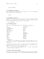
3.3.27 Material table
There is a set of predefined materials for use in elements such as collimators, e.g.
“Air”
“Aluminium”
“BeamGasPlugMat”
“Beryllium”
“CarbonMonoxide”
“CarbonSteel”
“Concrete”
“Copper”
“Graphite”
“Invar”
“Iron”
“LaserVac”
“Lead”
“LeadTungstate”
“LiquidHelium”
“NbTi”
“Niobium”
“Silicon”
“SmCo”
“Soil”
“Titanium”
“TitaniumAlloy”
“Tungsten”
“Vacuum”
“Vanadium”
“Water”
“WeightIron”
Currently “Air”, “CarbonMonoxide” and “Vacuum” are gas at T=300K, p=10−12 bar:
both “Air” and “Vacuum” are a N(80):O(20) mixture, “CarbonMonoxide is composed of
CO molecules.
There are also predefined elements (i.e. atoms) that can be used for building composite
materials: "H", "He", "Be", "C" , "N", "O", "Al", "Si", "P" , "S", "Ca", "Ti", “V" ,
"Mn", "Fe", "Co", "Ni", "Cu", "Nb", "Sm", "W" , "Pb".
For more details see the file src/BDSMaterials.cc or run the command bdsim
--materials from the command line.
3.4 Run control and output
The execution control is performed in the GMAD input file through option and sample
commands. How the results are recorded is controlled by the sample command. When the
Chapter 3: Lattice description
17
visualization is turned on, it is also controlled through Geant4 command prompt
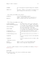
3.4.1 option
Most of the options in bdsim are set up by the command
option, <name>=value, ...;
The following options influence the geometry:
beampipeRadius
default beampipe outer radius [m]
beampipeThickness
default beampipe thickness [m]
beampipeMaterial
default beampipe material
apertureType
aperture model to use, one of circular, rectangular and
elliptical. Circular is the default.
aper1
aperture parameter 1 [m]. Typically x size.
aper2
aperture parameter 2 [m].
aper3
aperture parameter 3 [m].
aper4
aperture parameter 4 [m].
boxSize
default accelerator component full width [m]
vacuumMaterial
the beam pipe gas material (default “Vacuum”, which is composed of 48.2% H, 22.1% C and 29.7% O, and has a temperature of 300K)
vacuumPressure
the pressure of the beam pipe gas in bar (default 1e-12)
buildTunnel
whether to build a tunnel (default=0)
buildTunnelFloor
whether to add a floor to the tunnel (default=0)
tunnelRadius
tunnel radius [m]
tunnelThickness
the thickness of the tunnel wall [m]
tunnelSoilThickness
the thickness of the soil surrounding the tunnel [m]
tunnelMaterial
the material of the tunnel (default concrete)
soilMaterial
the material of the soil surrounding the tunnel (default soil)
tunnelOffsetX
the horizontal offset of the tunnel with respect to the beam
line
tunnelOffsetY
the vertical offset of the tunnel with respect to the beam line
tunnelFloorOffset
the offset of the tunnel floor from the centre of the tunnel
samplerDiameter
the diameter of the sampler planes (default is 2 times
tunnelRadius)
blmRad
the radius of the beam loss monitor cylinders
blmLength
the lengths of the beam loss monitor cylinders
includeIronMagFields
whether to include the magnetic fields in the magnet iron
(default=1)
The following options influence the tracking:
maximumTrackingTime
maximum tracking time for entire simulation
deltaChord
chord finder precision
deltaIntersection
boundary intersection precision
Chapter 3: Lattice description
chordStepMinimum
lengthSafety
minimumEpsilonStep
maximumEpsilonStep
deltaOneStep
18
minimum step size
element overlap safety
minimum relative error acceptable in stepping
maximum relative error acceptable in stepping
set position error acceptable in an integration steps
The following options influence the physics:
physicsList
thresholdCutCharged
thresholdCutPhotons
stopTracks
synchRadOn
srTrackPhotons
srLowX
srLowGamE
srMultiplicity
prodCutPhotons
prodCutPhotonsP
prodCutPhotonsA
prodCutElectrons
prodCutElectronsP
prodCutElectronsA
prodCutPositrons
prodCutPositronsP
prodCutPositronsA
turnOnCerenkov
defaultRangeCut
gammaToMuFe
annihiToMuFe
eetoHadronsFe
determines the set of physics processes used
charged particle cutoff energy
photon cutoff energy
if set, tracks are terminated after interaction
with material and energy deposit recorded
turn on Synchrotron Radiation process
whether to track the SR photons
sets lowest energy of SR to X*E critical
lowest energy of propagating SR photons
a factor multiplying the number of synchrotron radiation
photons
standard overall production cuts for photons (default 0.7 mm)
precision production cuts for photons in the precision region
(default 0.7 mm)
precision production cuts for photons in the approximation
region (default 1 m)
standard overall production cuts for electrons (default 0.7
mm)
precision production cuts for electrons in the precision region
(default 0.7 mm)
precision production cuts for electrons in the approximation
region (default 1 m)
standard overall production cuts for positrons (default 0.7
mm)
precision production cuts for positrons in the precision region
(default 0.7 mm)
precision production cuts for positrons in the approximation
region (default 1 m)
if set, Cerenkov radiation is turned on
the default predicted range at which a particle is cut. Default
is 0.7mm
the cross section enhancement factor for the gamma to muon
process
the cross section enhancement factor for the electron-positron
annihilation to muon process
the cross section enhancement factor for the electron-positron
annihilation to hadrons process
Chapter 3: Lattice description
useEMLPB
LPBFraction
19
if set, electromagnetic lead particle biasing is used. Default is
0
the fraction of EM processes in which electromagnetic lead
particle biasing is used, from 0.0=never to 1.0=always
The following options influence the generation:
randomSeed
ngenerate
seed for the random number generator;
setting to -1 uses the system clock to generate the seed
number of primary particles fired when in batch mode
The following options influence the output
elossHistoBinWidth
sensitiveBeamlineComponents
sensitiveBeamPipe
sensitiveBLMs
storeTrajectory
storeMuonTrajectories
storeNeutronTrajectories
trajCutGTZ
trajCutLTR
bin width in metres for the energy loss histogram
if set, energy losses in beamline components are
recorded in the energy loss histogram. Set by default
if set, energy losses in the beam pipe are recorded in
the energy loss histogram. Set by default
if set, energy losses in the beam loss monitors are
recorded in the energy loss histogram. Set by default
if set, the trajectories are stored in the root file
if set, the muon trajectories are stored in the root
file
if set, the neutron trajectories are stored in the root
file
do not store any trajectories who end less than this
z distance
do not store any trajectories who end outside of this
radius
Miscellaneous options:
nperfile
nlinesIgnore
number of events recorded per file in ROOT output
number of lines to skip when reading bunch files
For a more detailed description of how the option influence the tracking see Chapter 5
[Physics], page 25
3.4.2 beam
The parameters related to the beam are set with the beam command
beam, <name>=value, ...;
Chapter 3: Lattice description
20
There is a set of predefined distribution types that can be generated10 . In this case one
needs to specify the following parameters:
• particle - particle name, "e-","e+","gamma","proton", etc
• energy - particle energy
• distrType - type of distribution
and, in addition, other parameters that depend on the distribution type that has been
chosen:
1. Global options:
• X0 - Offset of distribution centre in x[m]
• Y0 - Offset of distribution centre in y[m]
• Z0 - Offset of distribution centre in z[m]
• Xp0 - Angular offset from nominal axis in x-z plane
• Yp0 - Angular offset from nominal z axis in y-z plane
• Zp0 - Directional flag: Zp0 < 0 points the particle back up the beamline
• T0 - Global time offset [s]
2. distrType=”reference”: a reference orbit particle, which has the offsets in the global
options so
• X0 - Offset of distribution centre in x[m]
• Y0 - Offset of distribution centre in y[m]
• Z0 - Offset of distribution centre in z[m]
• Xp0 - Angular offset from nominal axis in x-z plane
• Yp0 - Angular offset from nominal z axis in y-z plane
• Zp0 - Directional flag: Zp0 < 0 points the particle back up the beamline
• T0 - Global time offset [s]
3. distrType=”gauss”: a gaussian in x, x’, y, y’, energy and time, with given widths:
• sigmaX - RMS of x distribution in [m]
• sigmaXp - RMS of x’ distribution in [rad]
• sigmaY - RMS of y distribution in [m]
• sigmaYp - RMS of y’ distribution in [rad]
• sigmaE - RMS of energy distribution divided by nominal beam kinetic energy
• sigmaT - RMS of time distribution in [s]
4. distrType=”gausstwiss”: a gaussian bunch defined by twiss parameters [4], emittance,
energy and time:
• betx - βx in [m]
• bety - βy in [m]
• alfx - αx
• alfy - αy
• emitx - x in [m]
10
see src/BDSBunch.cc for more details
Chapter 3: Lattice description
21
• emity - y in [m]
• sigmaE - RMS of energy distribution divided by nominal beam kinetic energy
• sigmaT - RMS of time distribution in [s]
5. distrType=”gaussmatrix”: a gaussian bunch defined by N (N −1)/2 elements of sigma
matrix, this overwrites sigmaX, sigmaXp, sigmaY, sigmaYp, sigmaE and sigmaT variables if they have been defined previously. It will also recalculate the Twiss parameters.
• sigmaMN - σM N in [m] where M range between 1 and 6 and N ranges between M and
6
6. distrType=”eshell”: a thin elliptic shell (locus) in x,x’ and y,y’ with given semiaxes:
• shellX - radius in [m]
• shellXp - radius in [rad]
• shellY - radius in [m]
• shellYp - radius in [rad]
• sigmaE - in [GeV]
The width of shell can also be specifed via the following parameters:
• shellXWidth - absolute width in [m]
• shellXpWidth - absolute width in [rad]
• shellYWidth - absolute width in [m]
• shellYpWidth - absolute width in [rad]
If left unspecified, these default to 0 and therefore the shell is infinitely thin. Partilces
are uniformly distributed in this width.
7. distrType=“ring”: in the x, y plane the particles are uniformly distributed in r and
in φ inside a ring with inner radius Rmin and outer radius Rmax. x’, y’ and time are
exactly Xp0,Yp0 and T0 respectively for each generated particle. The kinetic energy
distribution is a gaussian of width sigmaE centered about the nominal beam kinetic
energy.
• Rmin, Rmax - inner and outer radius in [m]
• sigmaE - RMS energy spread [GeV]
8. distrType=“circle”: filled circle in both x,x’ and y,y’ planes with uniform distribution in all dimensions. The input parameters specify a radius R that is the same for
both x,x’ and y,y’, but it is denoted in input as X.
• envelopeX - radius in x, y - in [m]
• envelopeXp - radius in x’, y’ - in [rad]
• envelopeT - full width in time - in [s]
• envelopeE - full width in energy - in [GeV]
9. distrType=“square”: similar to circle - a filled square in both x,x’ and y,y’ planes
with uniform distribution in all dimensions. The input parameters specify the envelope.
• envelopeX - half width of square in x - in [m]
• envelopeXp - half width of square in x’ - in [rad]
• envelopeY - half width of square in y - in [m]
Chapter 3: Lattice description
22
• envelopeYp - half width of square in y’ - in [rad]
• envelopeT - full with in time - in [s]
• envelopeE - full width in energy - in [GeV]
10. distrType=“userfile”: user defined file format and list of particles in ascii text file.
• distrFile - string (must be in inverted commas) filename where particles are
listed
• distrFileFormat = string specifying columns in text file
You must also specify the general option in your gmad file (ie not under beam.
option, nlinesIgnore = N;
where N is the integer number of liens to ignore in the file (for header purposes) default 0.
Examples:
beam, particle="e+",
energy=100*MeV,
distrType="gauss",
sigmaX=0.01,
sigmaXp=0.1,
sigmaY=0.01,
sigmaYp=0.1;
beam,
particle="e-",
energy = 1*GeV,
distrType = "userfile",
distrFile = "9_UserFile.dat",
distrFileFormat = "x[mum]:xp[mrad]:y[mum]:yp[mrad]:z[cm]:E[MeV]";
option, nlinesIgnore = 0;
Note, currently this distribution only works when bdsim is executed in
the directory of the userfile.
There are examples for all distribution types in
bdsimsource/test/BDSBunchTestFiles.
In alternative, one can pass to the simulation a file containing a list of particles to be
generated. For more details see Appendix C [Bunch description formats], page 36 [DEPRECATED].
3.4.3 sample and csample
To record the tracking results one uses the sample and csample commands. To insert a
sampling plane before <element> the following command should be used:
sample, range=<element>;
Example:
sample, range=d;
Chapter 3: Lattice description
23
To put a cylindrical sampler of length l0 (in [m]) around element <element> at distance
r0 (in [m]) the following command should be used:
csample, range=<element>, r=r0, l=l0;
Samplers output the following parameters at the specified location:
E
X
Y
Z
Xp
Yp
Zp
x
y
z
xp
yp
zp
nEvent
Energy[GeV]
Global X position
Global Y position
Global Z position
Global angle in x-z
Global angle in y-z
1-sqrt(Xp2 +Yp2 )
Relative x position
Relative y position
Relative z position11
Relative angle in x-z
Relative angle in y-z
1-sqrt(xp2 +yp2 )
Event number
E0
s
t
t0
trackID
weight
parentID
x0
y0
z0
xp0
yp0
zp0
partID
Energy at last scatter[Gev]
path length
time of flight
time of flight at last scatter
trackID of particle
weight of track
trackID of parent particle
x at last scatter
y at last scatter
z at last scatter
xp at last scatter
yp at last scatter
xp at last scatter
PDG particle identifier
3.4.4 dump
Used in conjunction with option,fifo=<filename> to output the bunch distribution at
a given point. If the specified output file is a FIFO, the distribution can be modified by
an external program before being piped back in to continue tracking. This is useful for
including multi-particle effects such as wakefields at given points in the lattice.
dump,range=dumpMarker1
option,fifo="/tmp/temp.dat"
Output is in the standard Guineapig format, with a header line stating the number of
particles to be output. The file to be read back should be in the same format as this.
3.4.5 use
use command selects the beam line for study
use, period=l1,range=q1/q2
3.4.6 print
The print command will print the element list. It can also print the value of an option or
a variable.
print, x;
11
See Appendix D [Known Issues], page 37
Chapter 4: Visualization
24
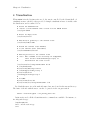
4 Visualization
When BDSIM is invoked in interactive mode, the run is controlled by the Geant4 shell. A
visualization macro should be then provided. A simple visualization macro is include with
the distribution, and is outlined below.
# Invoke the OGLSX driver
# Create a scene handler and a viewer for the OGLSX driver
/vis/open OGLIX
# Create an empty scene
/vis/scene/create
# Add detector geometry to the current scene
/vis/scene/add/volume
# Attach the current scene handler
# to the current scene (omittable)
/vis/sceneHandler/attach
# Add trajectories to the current scene
# Note: This command is not necessary in exampleN03,
#
since the C++ method DrawTrajectory() is
#
described in the event action.
/vis/viewer/set/viewpointThetaPhi 90 90
# /vis/drawVolume
#/vis/scene/add/trajectories
# /tracking/storeTrajectory 0
#/vis/viewer/zoom
/tracking/storeTrajectory 1
#
# for BDS:
#/vis/viewer/zoom 300
#/vis/viewer/set/viewpointThetaPhi 3 45
By default the macro is read from the file named vis.mac located in the current directory.
The name of the file with the macro can also be passed via the vis_mac switch.
bdsim --file=line.gmad --vis_mac=my_macro.mac
In interactive mode all the Geant4 interactive commands are available. For instance, to
fire 100 particles type
/run/beamOn 100
and to end the session type
exit
Chapter 5: Physics
25
To display help menu
/help;
For more details see [1].
5 Physics
BDSIM can exploit all physics processes that come with Geant4. In addition fast tracking
inside multipole magnets is provided. More detailed description of the physics is given
below.
5.1 physicsList option
Depending on for what sort of problem BDSIM is used, different sorts of physics processes
should be turned on. This processes are grouped into so called “physics lists”. The physics
list is specified by the physicsList option in the input file, e.g.
option, physicsList="em_standard";
Several predefined physics lists are available. Some physics lists allow biasing and reweighting for some processes e.g. muon production. To set the amount of biasing see
Section 3.4.1 [option], page 17. Further details of the QGSP, FTFP and BERT hadronic
physics lists can be found in [5].
standard
em_standard
em_low
em_muon
lw
merlin
hadronic_standard
hadronic_muon
hadronic_QGSP_BERT
hadronic_QGSP_BERT_
muon
hadronic_QGSP_BERT_HP_
muon
transportation of primary particles only
transportation
of
primary
particles,
ionization,
bremsstrahlung, Cerenkov, multiple scattering
the same but using low energy electromagnetic models
em standard plus muon production processes with biased
muon cross-sections
list for laser wire simulation - standard electromagnetic
physics and "laser wire" physics which is Compton Scattering
with total cross-section renormalized to 1.
transportation of primary particles, and the following processes for electrons: multiple scattering, ionisation, and
bremsstrahlung
em_standard plus fission, neutron capture, neutron and proton elastic and inelastic scattering
hadronic_standard plus muon production processes with biased muon cross-sections
em_standard plus hadron physics using the quark gluon string
plasma (QGSP) model and the Bertini cascade model (BERT)
hadron_QGSP_BERT plus muon production processes with biased muon cross-sections
hadron_QGSP_BERT_muon with high precision neutron
tracking
Chapter 6: Output Analysis
hadronic_FTFP_BERT
hadronic_FTFP_BERT_
muon
26
em_standard plus hadron physics using the Fritiof model followed by Reggion cascade and Precompound and evaporation
models for the nucleus de-excitation (FTFP) model and the
Bertini cascade model (BERT)
hadronic_FTFP_BERT plus muon production processes with
biased muon cross-sections
By default the standard physics List is used
5.2 Transportation
The transportation follows the scheme: the step length is selected which is defined either
by the distance of the particle to the boundary of the “logical volume” it is currently in
(which could be, e.g. field boundary, material boundary or boundary between two adjacent
elements) or by the mean free path of the activated processes. Then the particle is pushed to
the new position and secondaries are generated if necessary. Each volume has an associated
transportation algorithm. For an on-energy particle travelling close to the optical axis of a
quadrupole, dipole or a drift, standard matrix transportation algorithms are used [4]. For
multipoles of higher orders and for off-axis/energy particles Runge-Kutta methods are used.
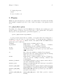
5.3 Tracking accuracy
The following options influence the tracking accuracy
chordStepMinimum
minimum chord length for the step
deltaIntersection
determines the precision of locating the point of intersection
of the particle trajectory with the boundary and hence the
error in the path length in each volume. This may influence
the results especially in the case when EM fields are present.
deltaChord
lengthSafety
all volumes will have an additional overlap of this length
thresholdCutCharged
energy below which charged particles are not tracked
thresholdCutPhotons
energy below which photons are not tracked
6 Output Analysis
During the execution the following things are recorded:
• energy deposition along the beamline
• sampler hits
If the output format is ASCII i.e. if BDSIM was invoked with the --output=ascii option,
then the output file “output.txt” containing the hits will be written which has rows like
#hits PDGtype p[GeV/c] x[micron] y[micron] z[m] x’[microrad] y’[microrad]
11 250 -4.72907 -5.86656 5.00001e-06 0 0
11 250 -8.17576 -4.99729 796.001 0.320334 -0.126792
If ROOT output is used then the root files output_0.root, output_1.root etc. will
be created with each file containing the number of events given by nperfile option. The
Appendix A: Geometry description formats
27
file contains the energy loss histogram and a tree for every sampler in the line with selfexplanatory branch names.
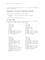
Appendix A Geometry description formats
The element with user-defined physical geometry is defined by
<element_name> : element, geometry=format:filename, attributes
for example,
colli : element, geometry="gmad:colli.geo"
A.1 gmad format
gmad is a simple format used as G4geometry wrapper. It can be used for specifying more
or less simple geometries like collimators. Available shapes are:
Box {
x0=x_origin,
y0=y_origin,
z0=z_origin,
x=xsize,
y=ysize,
z=zsize,
phi=Euler angle for rotation,
theta=Euler angle for rotation,
psi=Euler angle for rotation,
material=MaterialName
}
Tubs {
x0=x_origin,
y0=y_origin,
z0=z_origin,
rmin=inner radius,
rmax=outer radius,
z=zsize,
phi=Euler angle for rotation,
theta=Euler angle for rotation,
psi=Euler angle for rotation,
material=MaterialName
}
Cons {
x0=x_origin,
y0=y_origin,
z0=z_origin,
rmin1=inner radius at start,
rmax1=outer radius at start,
rmin2=inner radius at end,
rmax2=outer radius at end,
z=zsize,
material=MaterialName,
phi=Euler angle for rotation,
theta=Euler angle for rotation,
psi=Euler angle for rotation,
phi0=angle for start of sector,
dphi=angle swept by sector
}
Trd {
x0=x_origin,
y0=y_origin,
z0=z_origin,
x1=half length at wider side,
x2=half length at narrower side,
y1=half length at wider side,
y2=half length at narrower side,
z=zsize,
phi=Euler angle for rotation,
theta=Euler angle for rotation,
psi=Euler angle for rotation,
material=MaterialName
}
Appendix A: Geometry description formats
28
A file can contain several objects which will be placed sequentially into the volume, A
user has to make sure that there is no overlap between them.
A.2 mokka
As well as using the GMAD format to describe user-defined physical geometry it is also
possible to use a Mokka style format. This format is currently in the form of a dumped
MySQL database format - although future versions of BDSIM will also support online
querying of MySQL databases. Note that throughout any of the Mokka files, a # may be
used to represent a commented line. There are three key stages, which are detailed in the
following sections, that are required to setting up the Mokka geometry:
• Describing the geometry
• Creating a geometry list
• Defining a Mokka Element to load geometry descriptions from a list
A.2.1 Describing the geometry
An object must be described by creating a MySQL file containing commands that would
typically be used for uploading/creating a database and a corresponding new table into a
MySQL database. BDSIM supports only a few such commands - specifically the CREATE
TABLE and INSERT INTO commands. When writing a table to describe a solid there are
some parameters that are common to all solid types (such as NAME and MATERIAL) and some
that are more specific (such as those relating to radii for cone objects). A full list of the
standard and specific table parameters, as well as some basic examples, are given below
with each solid type. All files containing geometry descriptions must have the following
database creation commands at the top of the file:
DROP DATABASE IF EXISTS DATABASE_NAME;
CREATE DATABASE DATABASE_NAME;
USE DATABASE_NAME;
A table must be created to allow for the insertion of the geometry descriptions. A table
is created using the following, MySQL compliant, commands:
CREATE TABLE TABLE-NAME_GEOMETRY-TYPE (
TABLE-PARAMETER
VARIABLE-TYPE,
TABLE-PARAMETER
VARIABLE-TYPE,
TABLE-PARAMETER
VARIABLE-TYPE
);
Once a table has been created values must be entered into it in order to define the solids
and position them. The insertion command must appear after the table creation and must
the MySQL compliant table insertion command:
INSERT INTO TABLE-NAME_GEOMETRY-TYPE VALUES(value1, value2, "char-value",
...);
Appendix A: Geometry description formats
29
The values must be inserted in the same order as their corresponding parameter types
are described in the table creation. Note that ALL length types must be specified in mm
and that ALL angles must be in radians.
An example of two simple boxes with no visual attributes set is shown below. The first
box is a simple vacuum cube whilst the second is an iron box with length x = 10mm,
length y = 150mm, length z = 50mm, positioned at x=1m, y=0, z=0.5m and with zero
rotation.
CREATE TABLE mytable_BOX (
NAME
VARCHAR(32),
MATERIAL
VARCHAR(32),
LENGTHX
DOUBLE(10,3),
LENGTHY
DOUBLE(10,3),
LENGTHZ
DOUBLE(10,3),
POSX
DOUBLE(10,3),
POSY
DOUBLE(10,3),
POSZ
DOUBLE(10,3),
ROTPSI
DOUBLE(10,3),
ROTTHETA
DOUBLE(10,3),
ROTPHI
DOUBLE(10,3)
);
INSERT INTO mytable_BOX VALUES("a_box","vacuum", 50.0, 50.0, 50.0, 0.0, 0.0,
0.0, 0.0, 0.0, 0.0);
INSERT INTO mytable_BOX VALUES("another_box","iron", 10.0, 150.0, 50.0,
1000.0, 0.0, 500.0, 0.0, 0.0, 0.0);
Further examples of the Mokka geometry implementation can be found in the examples/Mokka/General directory. See the common table parameters and solid type sections
below for more information on the table parameters available for use.
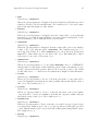
A.2.1.1 Common Table Parameters
The following is a list of table parameters that are common to all solid types either as an
optional or mandatory parameter:
Appendix A: Geometry description formats
30
• NAME
Variable type: VARCHAR(32)
This is an optional parameter. If supplied, then the Geant4 LogicalVolume associated
with the solid will be labelled with this name. The default is set to be the table’s name
plus an automatically assigned volume number.
• MATERIAL
Variable type: VARCHAR(32)
This is an optional parameter. If supplied, then the volume will be created with this
material type - note that the material must be given as a character string inside double
quotation marks(“). The default material is set as Vacuum.
• PARENTNAME
Variable type: VARCHAR(32)
This is an optional parameter. If supplied, then the volume will be placed as a daughter
volume to the object with ID equal to PARENTNAME. The default parent is set to be
the Component Volume. Note that if PARENTID is set to the Component Volume then
POSZ will be defined with respect to the start of the object. Else POSZ will be defined
with respect to the center of the parent object.
• INHERITSTYLE
Variable type: VARCHAR(32)
This is an optional parameter to be used with PARENTNAME. If set to “SUBTRACT“
then the instead of placing the volume within the parent volume as an inherited object,
it will be subtracted from the parent volume in a Boolean solid operation. The default
for this value is set to ““ - which sets to the usual mother/daughter volume inheritance.
• ALIGNIN
Variable type: INTEGER(11)
This is an optional parameter. If set to 1 then the placement of components will be
rotated and translated such that the incoming beamline will pass through the z-axis of
this object. The default is set to 0.
• ALIGNOUT
Variable type: INTEGER(11)
This is an optional parameter. If set to 1 then the placement of the next beamline
component will be rotated and translated such that the outgoing beamline will pass
through the z-axis of this object. The default is set to 0.
• SETSENSITIVE
Variable type: INTEGER(11)
This is an optional parameter. If set to 1 then the object will be set up to register energy
depositions made within it and to also record the z-position at which this deposition
occurs. This information will be saved in the ELoss Histogram if using ROOT output.
The default is set to 0.
• MAGTYPE
Variable type: VARCHAR(32)
Appendix A: Geometry description formats
31
This is an optional parameter. If supplied, then the object will be set up to produce
the appropriate magnetic field using the supplied K1 or K2 table parameter values .
Three magnet types are available - “QUAD”, “SEXT” and “OCT”. The default is set
to no magnet type. Note that if MAGTYPE is set to a value whilst K1/K2/K3 are not set,
then no magnetic field will be implemented.
• K1
Variable type: DOUBLE(10,3)
This is an optional parameter. If set to a value other than zero, in conjunction with
MAGTYPE set to “QUAD” then a quadrupole field with this K1 value will be set up within
the object. Default is set to zero.
• K2
Variable type: DOUBLE(10,3)
This is an optional parameter. If set to a value other than zero, in conjunction with
MAGTYPE set to “SEXT” then a sextupole field with this K2 value will be set up within
the object. Default is set to zero.
• K3
Variable type: DOUBLE(10,3)
This is an optional parameter. If set to a value other than zero, in conjunction with
MAGTYPE set to “OCT” then a sextupole field with this K3 value will be set up within
the object. Default is set to zero.
• POSX, POSY, POSZ
Variable type: DOUBLE(10,3)
These are required parameters. They are form the position in mm used to place the
object in the component volume. POSX and POSY are defined with respect to the center
of the component volume and with respect to the component volume’s rotation. POSZ
is defined with respect to the start of the component volume. Note that if the object
is being placed inside another volume using PARENTNAME then the position will refers
to the center of the parent object.
• ROTPSI, ROTTHETA, ROTPHI
Variable type: DOUBLE(10,3)
These are optional parameters. They are the Euler angles in radians used to rotate the
object before it is placed. The default is set to zero for each angle.
• RED, BLUE, GREEN
Variable type: DOUBLE(10,3)
These are optional parameters. They are the RGB colour components assigned to the
object and should be a value between 0 and 1. The default is set to zero for each colour.
• VISATT
Variable type: VARCHAR(32)
This is an optional parameter. This is the visual state setting for the object. Setting
this to “W” results in a wireframe displayment of the object. “S” produces a shaded
solid and “I” leaves the object invisible. The default is set to be solid.
Appendix A: Geometry description formats
32
• FIELDX, FIELDY, FIELDZ
Variable type: DOUBLE(10,3)
These are optional parameters. They can be used to apply a uniform field to any
volume, with default units of Tesla. Note that if there is a solenoid field present
throughout the entire element then this uniform field will act in addition to the solenoid
field.
• APPROXIMATIONREGION
Variable type: INTEGER(11)
This optional parameter, when set to 1, assigns the colume to the approximation region,
which has its own user defined electromagnetic production cuts (see Chapter 5 [Physics],
page 25, Section 3.3 [Physical elements], page 4).
A.2.1.2 ’Box’ Solid Types
Append _BOX to the table name in order to make use of the G4Box solid type. The following
table parameters are specific to the box solid:
• LENGTHX, LENGTHY, LENGTHZ
Variable type: DOUBLE(10,3)
These are required parameters. There values will be used to specify the box’s dimensions.
A.2.1.3 ’Trapezoid’ Solid Types
Append _TRAP to the table name in order to make use of the G4Trd solid type - which
is defined as a trapezoid with the X and Y dimensions varying along z functions. The
following table parameters are specific to the trapezoid solid:
• LENGTHXPLUS
Variable type: DOUBLE(10,3)
This is a required parameter. This value will be used to specify the x-extent of the
box’s dimensions at the surface positioned at +dz.
• LENGTHXPMINUS
Variable type: DOUBLE(10,3)
This is a required parameter. This value will be used to specify the x-extent of the
box’s dimensions at the surface positioned at -dz.
• LENGTHYPLUS
Variable type: DOUBLE(10,3)
This is a required parameter. This value will be used to specify the y-extent of the
box’s dimensions at the surface positioned at +dz.
• LENGTHYPMINUS
Variable type: DOUBLE(10,3)
This is a required parameter. This value will be used to specify the y-extent of the
box’s dimensions at the surface positioned at -dz.
• LENGTHZ
Variable type: DOUBLE(10,3)
Appendix A: Geometry description formats
33
This is a required parameter. This value will be used to specify the z-extent of the
box’s dimensions.
A.2.1.4 ’Cone’ Solid Types
Append _CONE to the table name in order to make use of the G4Cons solid type. The
following table parameters are specific to the cone solid:
• LENGTH
Variable type: DOUBLE(10,3)
This is a required parameter. This value will be used to specify the z-extent of the
cone’s dimensions.
• RINNERSTART
Variable type: DOUBLE(10,3)
This is an optional parameter. If set then this value will be used to specify the inner
radius of the start of the cone. The default value is zero.
• RINNEREND
Variable type: DOUBLE(10,3)
This is an optional parameter. If set then this value will be used to specify the inner
radius of the end of the cone. The default value is zero.
• ROUTERSTART
Variable type: DOUBLE(10,3)
This is a required parameter. This value will be used to specify the outer radius of the
start of the cone.
• ROUTEREND
Variable type: DOUBLE(10,3)
This is a required parameter. This value will be used to specify the outer radius of the
end of the cone.
• STARTPHI
Variable type: DOUBLE(10,3)
This is an optional parameter. If set then this value will be used to specify the starting
angle of the cone. The default value is zero.
• DELTAPHI
Variable type: DOUBLE(10,3)
This is an optional parameter. If set then this value will be used to specify the delta
angle of the cone. The default value is 2*PI.
A.2.1.5 ’Torus’ Solid Types
Append _TORUS to the table name in order to make use of the G4Torus solid type. The
following table parameters are specific to the torus solid:
• RINNER
Variable type: DOUBLE(10,3)
This is an optional parameter. If set then this value will be used to specify the inner
radius of the torus tube. The default value is zero.
Appendix A: Geometry description formats
34
• ROUTER
Variable type: DOUBLE(10,3)
This is a required parameter. This value will be used to specify the outer radius of the
torus tube.
• RSWEPT
Variable type: DOUBLE(10,3)
This is a required parameter. This value will be used to specify the swept radius of the
torus. It is defined as being the distance from the center of the torus ring to the center
of the torus tube. For this reason this value should not be set to less than ROUTER.
• STARTPHI
Variable type: DOUBLE(10,3)
This is an optional parameter. If set then this value will be used to specify the starting
angle of the torus. The default value is zero.
• DELTAPHI
Variable type: DOUBLE(10,3)
This is an optional parameter. If set then this value will be used to specify the delta
swept angle of the torus. The default value is 2*PI.
A.2.1.6 ’Polycone’ Solid Types
Append _POLYCONE to the table name in order to make use of the G4Polycone solid type.
The following table parameters are specific to the polycone solid:
• NZPLANES
Variable type: INTEGER(11)
This is a required parameter. This value will be used to specify the number of z-planes
to be used in the polycone. This value must be set to greater than 1.
• PLANEPOS1, PLANEPOS2, ..., PLANEPOSN
Variable type: DOUBLE(10,3)
These are required parameters. These values will be used to specify the z-position of the
corresponding z-plane of the polycone. There should be as many PLANEPOS parameters
set as the number of z-planes. For example, 3 z-planes will require that PLANEPOS1,
PLANEPOS2, and PLANEPOS3 are all set up.
• RINNER1, RINNER2, ..., RINNERN
Variable type: DOUBLE(10,3)
These are required parameters. These values will be used to specify the inner radius of
the corresponding z-plane of the polycone. There should be as many RINNER parameters
set as the number of z-planes. For example, 3 z-planes will require that RINNER1,
RINNER2, and RINNER3 are all set up.
• ROUTER1, ROUTER2, ..., ROUTERN
Variable type: DOUBLE(10,3)
These are required parameters. These values will be used to specify the outer radius of
the corresponding z-plane of the polycone. There should be as many ROUTER parameters
set as the number of z-planes. For example, 3 z-planes will require that ROUTER1,
ROUTER2, and ROUTER3 are all set up.
Appendix A: Geometry description formats
35
• STARTPHI
Variable type: DOUBLE(10,3)
This is an optional parameter. If set then this value will be used to specify the starting
angle of the polycone. The default value is zero.
• DELTAPHI
Variable type: DOUBLE(10,3)
This is an optional parameter. If set then this value will be used to specify the delta
angle of the polycone. The default value is 2*PI.
A.2.1.7 ’Elliptical Cone’ Solid Types
Append _ELLIPTICALCONE to the table name in order to make use of the G4Ellipticalcone
solid type. The following table parameters are specific to the elliptical cone solid:
• XSEMIAXIS
Variable type: DOUBLE(10,3)
This is a required parameter. This value will be used to specify the Semiaxis in X.
• YSEMIAXIS
Variable type: DOUBLE(10,3)
This is a required parameter. This value will be used to specify the Semiaxis in Y.
• LENGTHZ
Variable type: DOUBLE(10,3)
This is a required parameter. This value will be used to specify the height of the
elliptical cone.
• ZCUT
Variable type: DOUBLE(10,3)
This is a required parameter. This value will be used to specify the upper cut plane
level.
Note that the above parameters are used to define an elliptical cone with the following
parametric equations (in the usual Geant4 way):
x = XSEMIAXIS * (LENGTHZ - u) / u * Cos(v)
Y = YSEMIAXIS * (LENGTHZ - u) / u * Sin(v)
z=u
where v is between 0 and 2*PI and u between 0 and h respectively.
A.2.2 Creating a geometry list
A geometry list is a simple file consisting of a list of file names that contain geometry
descriptions. This is the file that should be passed to the GMAD file when defining the
Mokka element. An example of a geometry list containing ’boxes.sql’ and ’cones.sql’ would
be:
# ’#’ symbols can be used for commenting out an entire line
/directory/boxes.sql
/directory/cones.sql
Appendix C: Bunch description formats
36
A.2.3 Defining a Mokka element in the GMAD file
The Mokka element can be defined by the following command:
<element_name> : element, geometry=format:filename, attributes
where format must be set to mokka and filename must point to a file that contains a
list of files that have the geometry descriptions.
for example,
collimator : element, geometry=mokka:coll_geomlist.sql
A.3 gdml
GDML is a XML schema for detector description. GDML will be supported as an external
format starting from next release.
Appendix B Field description formats
The element with user-defined magnetic field map is defined by the command
<element_name> : element, bmap=format:filename, attributes
for example,
colli : element, bmap=XY:colli.bmap
Supported formats are “mokka” and “XY”. In the latter case a text files must be specified, where each rows must have the following format: x y Bx By Bz
Appendix C Bunch description formats
For compatibility with other simulation codes following bunch formats can be read. For
example, to use the file distr.dat as input the beam definition should look like
beam, particle="e-",distrType="guineapig_bunch",distrFile="distr.dat"
The formats currently supported are listed below:12
• guineapig_bunch : E[GeV] x[mum] y[mum] z[mum] x’[murad] y’[murad]
• guineapig_slac : E[GeV] x’[rad] y’[rad] z[mum] x[nm] y[nm]
• guineapig_pairs : E[GeV] x’[rad] y’[rad] z’[rad] x[nm] y[nm] z[nm] (here a particle
with E>0 is assumed to be an electron and with E<0 a positron.)
• cain : ....
A custom distribution file format can be specified in the form
distrType="field1[unit1]:field1[unit1]:...
The allowed values for fields/units are: .....
For instance:
12
see src/BDSBunch.cc for more details
References
beam,
37
particle="e-",
energy=ener * GeV,
distrType="pt[1]:E[GeV]:xp[rad]:yp[rad]:z[mum]:x[nm]:y[nm]",
distrFile="bunches/beam.dat";
Appendix D Known Issues
Samplers attached to multiple instances of the same element incorrectly register hits only
from the first instance in all such samplers. For example:
drift1: drift, l=1*m;
mark1: marker;
line1: line=(mark1,drift1,mark1,drift1);
sample, range=mark1[1];
sample, range=mark1[2];
will incorrectly record hits at mark1[1] in the sampler attached to mark1[2]. To avoid
this, samplers should be attached to uniquely named elements.
There is a known issue with the z parameter output to samplers. As particle data is
output at the z location of the sampler, when the global position is transformed from global
to relative coordinates z is identically zero. For a description of a particle’s longitudinal
position in the bunch, please use the parameter s instead.
References
[1] Geant4 User’s Guide, http://geant4.cern.ch/support/userdocuments.shtml
[2] Root User’s Guide, http://root.cern.ch/drupal/content/users-guide
[3] MAD-X User’s Guide,
http://madx.web.cern.ch/madx/madX/doc/usrguide/uguide.html
[4] for example ’Basic course on Accelerator optics’ by Schmuesser, Rossbach, CERN
Accelerator school
[5] A. Ribon et. al., Status of GEANT4 hadronic physics for the simulation of LHC
experiments at the start of LHC physics program, CERN-LCGAPP-2010-02, July 20
2010