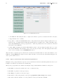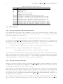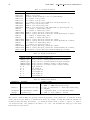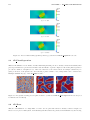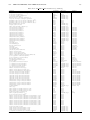
1
DL MESO USER MANUAL M. A. Seaton and W. Smith STFC Daresbury Laboratory Daresbury, Warrington, Cheshire, WA4 4AD United Kingdom Version 2.5, April 2012 Contents Contents 1 DL 1.1 1.2 1.3 1.4 1.5 1.6 1.7 1.8 2 The 2.1 2.2 2.3 2.4 2.5 MESO General Information Description . . . . . . . . . . . . . . Functionality . . . . . . . . . . . . . Requirements . . . . . . . . . . . . . The DL MESO Directory Structure Disclaimer . . . . . . . . . . . . . . . Copyright . . . . . . . . . . . . . . . Authors . . . . . . . . . . . . . . . . Suggestions and Bug Reports . . . . i . . . . . . . . . . . . . . . . . . . . . . . . . . . . . . . . . . . . . . . . . . . . . . . . . . . . . . . . DL MESO GUI Getting Started with the DL MESO GUI . . . . Lattice Boltzmann and the DL MESO GUI . . . Dissipative Particle Dynamics and the DL MESO Compiling and running DL MESO . . . . . . . . Notes . . . . . . . . . . . . . . . . . . . . . . . . . . . . . . . . . . . . . . . . 1 1 1 2 3 3 3 3 3 . . . . . . . . . . . . . . . . . . . . . . . . . . . . . . . . . . . . . . . . . . . . . . . . . . . . . . . . . . . . . . . . . . . . . . . . . . . . . . . . . . . . . . . . . . . . . . . . . . . . . . . . . . . . . . . . . . . . . . . . . . . . . . . . . . . . . . . . . . . . . . . . . . . . . . . . . . . . . . . . . . . . . . . . . . . . . . . . . . . . . . . . . . . . . . . . . . . . . . . . . . . . . . GUI . . . . . . . . . . . . . . . . . . . . . . . . . . . . . . . . . . . . . . . . . . . . . . . . . . . . . . . . . . . . . . . . . . . . . . . . . . . . . . . . . . . . . . . . . . . . . . . . . . . . . . . . . . . . . . . . . . . . . . . . . 5 . 5 . 6 . 12 . 18 . 19 I Lattice Boltzmann Equation (LBE) 21 3 The 3.1 3.2 3.3 3.4 3.5 3.6 23 23 23 24 25 26 27 Lattice Boltzmann Equation: Basic Theory Introduction . . . . . . . . . . . . . . . . . . . . . . Basic Definitions . . . . . . . . . . . . . . . . . . . Derivation of Equilibrium . . . . . . . . . . . . . . Structural Relaxation and Macroscopic Equations . Mesoscale Interaction . . . . . . . . . . . . . . . . Summary of Lattice Boltzmann Equation . . . . . . . . . . . . . . . . . . . . . . . . . . . . . . . . . . . . . . . . . . . . . . . . . . . . . . . . . . . . . . . . . . . . . . . . . . . . . . . . . . . . . . . . . . . . . . . . . . . . . . . . . . . . . . . . . . . . . . . . . . . . . . . . . . . . . . . . . . . . . . . . . . . . . . . . . . . . . . . . . 4 DL 4.1 4.2 4.3 MESO LBE Basic Definition 29 Lattice models . . . . . . . . . . . . . . . . . . . . . . . . . . . . . . . . . . . . . . . . . . . . . . 29 Data structure . . . . . . . . . . . . . . . . . . . . . . . . . . . . . . . . . . . . . . . . . . . . . . 36 The Parameters and Their Functions . . . . . . . . . . . . . . . . . . . . . . . . . . . . . . . . . . 39 5 DL 5.1 5.2 5.3 5.4 5.5 MESO LBE Features Collision and Propagation Algorithms Boundary conditions . . . . . . . . . . Mesoscale interactions . . . . . . . . . Diffusion and heat transfer . . . . . . Compressible and incompressible fluids . . . . . . . . . . . . . . . . . . . . . . . . . i . . . . . . . . . . . . . . . . . . . . . . . . . . . . . . . . . . . . . . . . . . . . . . . . . . . . . . . . . . . . . . . . . . . . . . . . . . . . . . . . . . . . . . . . . . . . . . . . . . . . . . . . . . . . . . . . . . . . . . . . . . . . . . . . . . . . . . . . . . . . 45 45 48 50 52 54 ii CONTENTS 6 DL MESO LBE Input and Output Files 55 6.1 Input files . . . . . . . . . . . . . . . . . . . . . . . . . . . . . . . . . . . . . . . . . . . . . . . . . 55 6.2 Output files . . . . . . . . . . . . . . . . . . . . . . . . . . . . . . . . . . . . . . . . . . . . . . . . 58 7 DL MESO LBE Package Reference 61 7.1 Overview . . . . . . . . . . . . . . . . . . . . . . . . . . . . . . . . . . . . . . . . . . . . . . . . . 61 7.2 DL MESO LBE Subroutines and Functions . . . . . . . . . . . . . . . . . . . . . . . . . . . . . . 62 8 DL MESO LBE Examples 8.1 2D Pressure . . . . . . . 8.2 2D Shear . . . . . . . . 8.3 2D CylinderFlow . . . . 8.4 2D KarmanVortex . . . 8.5 2D LidCavity . . . . . . 8.6 2D RayleighBenard . . . 8.7 2D DropShear . . . . . . 8.8 3D PhaseSeparation . . 8.9 3D Shear . . . . . . . . 8.10 3D RayleighBenard . . . . . . . . . . . . . . . . . . . . . . . . . . . . . . . . . . . . . . . . . . . . . . . . . . . . . . . . . . . . . . . . . . . . . . . . . . . . . . . . . . . . . . . . . . . . . . . . . . . . . . . . . . . . . . . . . . . . . . . . . . . . . . . . . . . . . . . . . . . . . . . . . . . . . . . . . . . . . . . . . . . . . . . . . . . . . . . . . . . . . . . . . . . . . . . . . . . . . . . . . . . . . . . . . . . . . . . . . . . . . . . . . . . . . . . . . . . . . . . . . . . . . . . . . . . . . . . . . . . . . . . . . . . . . . . . . . . . . . . . . . . . . . . . . . . . . . . . . . . . . . . . . . . . . . . . . . . . . . . . . . . . . . . . . . . . . . . . . . . . . . . . . . . . . . . . . . . . . . . . . . . . . . . . . . . . . . . . . . . . . . . . . . . . . . . . . . . . . . . . . . . . . . . . . . . . . II Dissipative Particle Dynamics (DPD) 9 Dissipative Particle Dynamics: Basic Theory 9.1 Introduction . . . . . . . . . . . . . . . . . . . . 9.2 Outline of Method . . . . . . . . . . . . . . . . 9.3 Equation of state and dynamic properties . . . 9.4 Derivation of Equilibrium . . . . . . . . . . . . 9.5 Summary of Dissipative Particle Dynamics . . 119 119 119 120 120 120 121 121 122 122 123 125 . . . . . . . . . . . . . . . . . . . . . . . . . . . . . . . . . . . . . . . . . . . . . . . . . . . . . . . . . . . . . . . . . . . . . . . . . . . . . . . . . . . . . . . . . . . . . . . . . . . . . . . . . . . . . . . . . . . . . . . . . . . . . . . . . . . . . . . . . . . . 127 127 127 129 129 130 10 DL MESO DPD Basic Definition 131 10.1 Data structure . . . . . . . . . . . . . . . . . . . . . . . . . . . . . . . . . . . . . . . . . . . . . . 131 10.2 The Parameters and Their Functions . . . . . . . . . . . . . . . . . . . . . . . . . . . . . . . . . . 134 11 DL MESO DPD Features 11.1 Domain decomposition and linked-list cell calculations 11.2 Thermostats and integration algorithms . . . . . . . . 11.3 Barostats . . . . . . . . . . . . . . . . . . . . . . . . . 11.4 Particle-particle interactions . . . . . . . . . . . . . . . 11.5 Long-ranged Electrostatic (Coulombic) Potentials . . . 11.6 Bond interactions between particles . . . . . . . . . . . 11.7 Surface interactions . . . . . . . . . . . . . . . . . . . . . . . . . . . . . . . . . . . . . . . . . . . . . . . . . . . . . . . . . . . . . . . . . . . . . . . . . . . . . . . . . . . . . . . . . . . . . . . . . . . . . . . . . . . . . . . . . . . . . . . . . . . . . . . . . . . . . . . . . . . . . . . . . . . . . . . . . . . . . . . . . . . . . . . . . . . . . . . . . . . . . . . . . . . . 141 141 142 145 147 150 152 155 12 DL MESO DPD Input and Output Files 157 12.1 Input files . . . . . . . . . . . . . . . . . . . . . . . . . . . . . . . . . . . . . . . . . . . . . . . . . 157 12.2 Output files . . . . . . . . . . . . . . . . . . . . . . . . . . . . . . . . . . . . . . . . . . . . . . . . 164 167 13 DL MESO DPD Package Reference 13.1 Overview . . . . . . . . . . . . . . . . . . . . . . . . . . . . . . . . . . . . . . . . . . . . . . . . . 167 13.2 DL MESO DPD Subroutines and Functions . . . . . . . . . . . . . . . . . . . . . . . . . . . . . . 168 14 DL MESO DPD Examples 215 14.1 Mixture Small . . . . . . . . . . . . . . . . . . . . . . . . . . . . . . . . . . . . . . . . . . . . . . . 215 CONTENTS 14.2 Mixture Large . . . . . 14.3 PhaseSeparation . . . . 14.4 Aggregate . . . . . . . . 14.5 Polyelectrolyte . . . . . 14.6 AmphiphileMesophases . 14.7 VesicleFormation . . . . 14.8 PoiseuilleFlow . . . . . . 14.9 ShearFlow . . . . . . . . 14.10VapourLiquid . . . . . . iii . . . . . . . . . . . . . . . . . . . . . . . . . . . . . . . . . . . . . . . . . . . . . . . . . . . . . . . . . . . . . . . . . . . . . . . . . . . . . . . . . . . . . . . . . . . . . . . . . . . . . . . . . . . . . . . . . . . . . . . . . . . . . . . . . . . . . . . . . . . . . . . . . . . . . . . . . . . . . . . . . . . . . . . . . . . . . . . . . . . . . . . . . . . . . . . . . . . . . . . . . . . . . . . . . . . . . . . . . . . . . . . . . . . . . . . . . . . . . . . . . . . . . . . . . . . . . . . . . . . . . . . . . . . . . . . . . . . . . . . . . . . . . . . . . . . . . . . . . . . . . . . . . . . . . . . . . . . . . . . . . . . . . . . . . . . . . . . . . . . . . . . . . . . . . . . . . . . . . . . . . . . . . . . . . 215 216 216 217 217 218 219 219 220 A Manual compiliation and running of DL MESO 221 A.1 DL MESO LBE . . . . . . . . . . . . . . . . . . . . . . . . . . . . . . . . . . . . . . . . . . . . . . 221 A.2 DL MESO DPD . . . . . . . . . . . . . . . . . . . . . . . . . . . . . . . . . . . . . . . . . . . . . 222 B DL MESO Utilities 225 B.1 DL MESO LBE . . . . . . . . . . . . . . . . . . . . . . . . . . . . . . . . . . . . . . . . . . . . . . 225 B.2 DL MESO DPD . . . . . . . . . . . . . . . . . . . . . . . . . . . . . . . . . . . . . . . . . . . . . 227 C DL MESO DPD Error Messages 231 D DL MESO Licence Agreement (Academic Purposes) 239 Bibliography 247 Acknowledgements DL MESO was developed under the auspices of the Engineering and Physical Sciences Research Council (EPSRC) for the EPSRC’s Collaborative Computational Project for the Computer Simulation of Condensed Phases (CCP5). The members of the CCP5 DL MESO consortium were: David M. Heyes, University of Surrey Chris M. Care, Sheffield Hallam University Peter V. Coveney, University College London David Emerson, STFC Daresbury Laboratory Rob English, North East Wales Institute Andrea Ferrante, Unilever Port Sunlight Ian Halliday, Sheffield Hallam University John Harding, University of Sheffield Sebastian Reich, Imperial College Bill Smith, STFC Daresbury Laboratory Patrick B. Warren, Unilever Port Sunlight Julia Yeomans, Oxford University Many other people have given advice and encouragement in the development of DL MESO. We gratefully acknowledge the support of the following people: Maurice Leslie, Richard Wain, Alexandre Dupuis, Jonathan Chin, Michael Dupin, Weiming Liu and John Purton. Particular thanks go to Rongshan Qin at Imperial College as the original author of the Lattice Boltzmann Equation source code (DL MESO LBE) and the DL MESO graphical user interface, and Richard Anderson at STFC Daresbury Laboratory and Ard van Bergen at Novidec for their contributions to the Dissipative Particle Dynamics source code (DL MESO DPD). v Chapter 1 DL MESO General Information 1.1 Description DL MESO is a general purpose mesoscopic simulation package developed at Daresbury Laboratory by Dr Michael Seaton under the auspices of the Engineering and Physical Sciences Research Council (EPSRC) for the EPSRC’s Collaborative Computational Project for the Computer Simulation of Condensed Phases (CCP5). The package is the property of the Science and Technology Facilities Council (STFC). DL MESO is issued free under licence to academic institutions pursuing scientific research of a non-commercial nature. All recipients of the code must first agree to the terms and conditions of the licence and register with us to be kept aware of new developments and discovered bugs. Commercial organisations interested in acquiring the package should approach the Scientific Computing Department, STFC Daresbury Laboratory in the first instance. Daresbury Laboratory is the sole centre for distribution of the package. Under no account is it to be redistributed to third parties without consent of the owners. DL MESO contains two mesoscale simulation methods: Lattice Boltzmann Equation (included with version 1.0 and later) Dissipative Particle Dynamics (included with version 2.0 and later) 1.2 Functionality The following is a list of the features that DL MESO currently supports. Users are reminded that we are interested in hearing what other features could be usefully incorporated. We obviously have ideas of our own and CCP5 strongly influences developments, but other input would be welcome nevertheless. 1.2.1 Lattice Boltzmann Equation DL MESO LBE can simulate lattice-gas systems using the Lattice Boltzmann Equation (LBE). The following properties and features are currently available: Multiple fluid components, solutes and coupled heat transfers[72] Collisions: Bhatnagar-Gross-Krook (BGK) single-relaxation-time[4] or Multiple-Relaxation-Time (MRT)[33, 8] Boundary conditions: Periodic, bounce-back (including stationary objects), constant pressure/velocity at planar surfaces[73] 1 2 CHAPTER 1. DL MESO GENERAL INFORMATION Mesoscale interactions: Shan-Chen pseudopotential method[55, 56], Lishchuk continuum-based method[35] Initial conditions can either be determined by DL MESO LBE or specified by the user 1.2.2 Dissipative Particle Dynamics DL MESO DPD can model DPD particles (‘beads’) with soft or hard potential fields, along with thermostatting dissipative and random forces. The following properties and features are currently available: Choice of integrators/thermostats: standard Velocity Verlet, DPD Velocity Verlet[13], Lowe-Andersen[36], Peters[47] and Stoyanov-Groot[62] Constant volume (NVT) or constant pressure (NPT) simulations with Berendsen[2] or Langevin[29] barostats User selection of interaction lengths, conservative and dissipative force parameters for each species and between unlike species Bond stretching, angles and dihedrals between beads in user-defined ‘molecules’ Potentials: standard Groot-Warren DPD[16], density-dependent (many-body) DPD[46, 66], LennardJones[30], Weeks-Chandler-Andersen[69] Electrostatic potentials between charged beads using a modified Ewald summation[14] Boundaries: Periodic, hard reflecting walls with optional short-range repulsions[50], frozen particle walls, Lees-Edwards periodic shearing boundaries[34] Initial conditions can either be determined by DL MESO DPD or specified by the user 1.3 1.3.1 Requirements Software requirements Standard C++ Compiler for LBE source code, DL MESO LBE Standard Fortran90 Compiler for DPD source code, DL MESO DPD Message Passing Interface (if parallel execution required) JAVA 2 Version 1.4 or higher (if GUI is to be used) GNU Make (included in standard Unix/Linux distributions; can be installed for Windows) 1.3.2 System requirements DL MESO is designed to work in both serial and parallel running; it can be run on standalone machines, clusters and supercomputers. The code has been tested on Solaris, Windows XP, IBM p690+ HPCx, PowerPC 450 Blue Gene/P and Cray XT4/XT6 HECToR machines. 1.4. THE DL MESO DIRECTORY STRUCTURE 1.4 3 The DL MESO Directory Structure The supplied version of DL MESO is a gzipped tar file, which unpacks as directory dl meso 2.x, where x is a generation number. Beneath the top level of this directory are a number of subdirectories: LBE - containing the LBE source code DPD - containing the DPD source code JAVA - containing the GUI source code MAN - containing the DL MESO user manual DEMO - containing test cases for DL MESO WORK - an example ‘working directory’ 1.5 Disclaimer Neither STFC, CCP5 nor any of the authors of the DL MESO package guarantee that the package is free from error. Neither do they accept responsibility for any loss or damage that results from its use. 1.6 Copyright © STFC Daresbury Laboratory 2012 1.7 Authors Dr Michael Seaton and Prof. William Smith Scientific Computing Department STFC Daresbury Laboratory Warrington WA4 4AD United Kingdom 1.8 Suggestions and Bug Reports We encourage users to send suggestions for improvements and new features for DL MESO, including bug reports and subroutines, as well as any additional test cases that demonstrate its features. All of these should be sent to [email protected] Chapter 2 The DL MESO GUI 2.1 Getting Started with the DL MESO GUI The DL MESO GUI offers a convenient way of using the DL MESO package, although it is not an essential tool for those who prefer command line operation: Appendix A provides details on compiling the DL MESO program codes manually. Working with the GUI requires the availability of Java tools, particularly the javac compiler and the java runner for Java 2 version 1.4 or later. These may be obtained from the java.sun.com website. To build the GUI, proceed as follows: Enter the DL MESO/JAVA directory. Type javac *.java to compile the source code. Type jar -cfm GUI.jar manifest.mf *.class to create the GUI.jar executable JAR file. Move to your working directory. Launch the GUI. A Unix/Linux script called makegui that performs the build of the GUI can be found in the JAVA subdirectory. Your working directory is the directory from which you wish to work when running DL MESO. Working there will keep any files you generate separate from the DL MESO source files. Note in the current version of DL MESO the working directory should be at the same directory level as the JAVA direction, i.e. within the DL MESO top directory, and contain the executables of any external utilities required to set up input files and gather or process output files from simulations. An example of such a working directory (called WORK) is present under the DL MESO top directory; this includes a makefile to compile all of the external utilties which can be invoked by the command make -f Makefile-utils. In your working directory you can start the GUI with the command java -jar ../JAVA/GUI.jar You may consider saving this command in a script for simple execution. An example script for Unix/Linux called rungui is present in the WORK subdirectory. Figure 2.1 shows the DL MESO GUI when it is started. Clicking the LBE and DPD buttons will produce the Lattice Boltzmann and Dissipative Particle Dynamics panels respectively, which will guide you through setting up input files, modifying and compiling the program code, running the simulation and gathering the results files 5 6 CHAPTER 2. THE DL MESO GUI Figure 2.1: DL MESO GUI on startup for plotting and visualization. The SPH button is for Smoothed Particle Hydrodynamic simulations, which will be included in future versions of DL MESO: clicking on this button will currently produce a warning message. This user manual can be read in Adobe Acrobat Reader (if installed) by clicking the Manual button, while Help will advise you to visit the DL MESO website at www.ccp5.ac.uk/DL MESO. 2.2 Lattice Boltzmann and the DL MESO GUI To access the LBE facilities in the DL MESO GUI, proceed as follows: Click the LBE button to get the LBE panel. Click the Define LBE System button and supply the required information. The file lbin.sys will be created by the step. Click the Set LBE Space button to define the simulation space. The file lbin.spa will be created by this step. 2.2.1 Defining the System Figure 2.2 shows the Define LBE System panel with the rows for data entry labelled in red numbering. The required data are as follows: 1. The required LBE model can be selected from the pull-down list: the D2Q9, D3Q15, D3Q19 and D3Q27 square lattice schemes are available. The tickbox can be selected to specify that the fluids in the system should be treated as incompressible. 2. The collision/forcing type for the system can be selected out of BGK, BGK with Guo forcing, MRT and MRT with Guo-like forcing. 2.2. LATTICE BOLTZMANN AND THE DL MESO GUI 7 Figure 2.2: Define LBE System 3. The required mesophase interactions can be selected from the pull-down list: currently available options include no interactions, Shan/Chen pseudopotential interactions, Shan/Chen interactions with surface wetting and Lishchuk continuum-based interactions. 4. The number of grid points sets the size of the system. For 2D systems, the number of grid points in the z direction must equal 1; selecting a two-dimensional lattice model greys out this box. 5. The total steps and the equilibration steps for the simulation. 6. the save span (number of timesteps between system outputs) and the boundary width for running the parallel version of DL MESO LBE are given in this row. (The serial version by default automatically resets the boundary width to zero.) 7. The output format for system snapshots is set using this pull-down list: VTK, Legacy VTK and Plot3D. 8. The sound speed (c) and kinetic viscosity (ν) are real-life quantities for the first (main) fluid. These do not influence calculations at all but allow conversions √between lattice and real units: the time step and respectively. lattice spacing are given by ∆t = c2 τ ν− 1 and ∆x = c τ 3ν ( f 2) ( f − 12 ) 9. The specified top boundary speed (in lattice units), i.e. at the maximum y value for the grid. This and similar properties only need to be specified if the boundary includes a fixed velocity; any specified value will be ignored for periodic, bounce-back and fixed density conditions. Note that the z-component will be greyed out for two-dimensional systems. 10. The specified bottom boundary speed (in lattice units), i.e. at the minimum y value for the grid. 11. The specified left boundary speed (in lattice units), i.e. at the minimum x value for the grid. 12. The specified right boundary speed (in lattice units), i.e. at the maximum x value for the grid. 13. The specified front boundary speed (in lattice units), i.e. at the maximum z value for the grid. For two-dimensional systems this can be omitted and is thus greyed out. 8 CHAPTER 2. THE DL MESO GUI 14. The specified back boundary speed (in lattice units), i.e. at the minimum z value for the grid. For two-dimensional systems this can be omitted and is thus greyed out. 15. The noise magnitude only has an effect for initializing multiple phase simulations. DL MESO LBE may include either a phase field parameter or no phase field parameter for systems with multiple phases; neither mesophase algorithm requires it and thus this option is currently disabled. 16. The number of fluids (phases) can be increased if a multiple fluid system is to be studied: up to 6 fluids may be modelled in DL MESO LBE. The parameters and boundary conditions for the fluid(s) must then be set by clicking the set fluid parameters button – see below for more details. 17. The number of solutes needs changing if solute parameters are required: if the number of solutes is greater than zero (and up to 6), the number of fluids in the above row must be set to 0 or 1. If used, the parameters and boundary conditions for the solutes must be set by clicking the set solute parameters button – see below for more details. 18. The using temperature scalar box may be clicked yes if thermal systems are to be studied. If checked, the thermal parameters must be set by clicking the set thermal parameters button – see below for more details. If a valid lbin.sys file already exists in the (current) working directory, the OPEN button can be clicked to load its information into the GUI, which can then be viewed and edited. Once all the data in this window and any pop-up windows for fluid, solute and thermal parameters are filled in, the SAVE button should be clicked to write the lbin.sys file. 2.2.1.1 Fluid, solute and thermal parameters Examples of the pop-up windows for fluid, solute and thermal parameters can be seen in Figure 2.3 with the rows labelled in red numbering: multiple columns of dialogue boxes are made available for systems with multiple fluids and/or solutes. For fluids, the required data are as follows: 1. Body force x-axis: the x-component of body force on each fluid. 2. Body force y-axis: the y-component of body force on each fluid. 3. Body force z-axis: the z-component of body force on each fluid. (Greyed out for two-dimensional systems.) 4. Boussinesq force x-axis: the x-component of the Boussinesq force parameter (~g β) on each fluid. 5. Boussinesq force y-axis: the y-component of the Boussinesq force parameter on each fluid. 6. Boussinesq force z-axis: the z-component of the Boussinesq force parameter on each fluid. (Greyed out for two-dimensional systems.) 7. The initial fluid densities are applied throughout the system and used to initialize LBE calculations. 8. The constant fluid density (ρ0 ) for incompressible systems: this property can also be used to define the reference densities for Shan/Chen pseudopotentials and for initialising systems with fluid drops. 9. The fluid densities at the top boundary. 10. The fluid densities at the bottom boundary. 11. The fluid densities at the left boundary. 2.2. LATTICE BOLTZMANN AND THE DL MESO GUI (a) Fluid parameters (b) Solute parameters 9 (c) Thermal parameters Figure 2.3: Fluid, solute and thermal parameter pop-up windows 12. The fluid densities at the right boundary. 13. The fluid densities at the front boundary. (Greyed out for two-dimensional systems.) 14. The fluid densities at the back boundary. (Greyed out for two-dimensional systems.) 15. The relaxation time (τf ) for each fluid: these values should be greater than 0.5 to give non-zero kinetic viscosities. 16. The bulk relaxation time (τf,bulk ) for each fluid: these values are only used in multiple-relaxation-time schemes to define the bulk viscosity and again should be greater than 0.5. 17. If more than one phase is being modelled, non-zero interaction parameters between the fluid species are required (gab ). The Shan/Chen algorithm can accept values of gab for both a = b and a 6= b, while the Lishchuk algorithm only requires gab for a 6= b. 18. If the Shan-Chen pseudopotential algorithm with wetting is to be used, wall interaction parameters between the fluid species and solid surfaces are required (ga,wall ). If the Lishchuk continuum-based algorithm is to be used, a non-zero segregation parameter (β) is required to ensure immiscible fluids separate out from each other. Solutes require the following data in the following row numbers: 1. The initial concentrations of the solutes throughout the system, as used for initialization. 10 CHAPTER 2. THE DL MESO GUI 2. The solute concentrations at the top boundary. 3. The solute concentrations at the bottom boundary. 4. The solute concentrations at the left boundary. 5. The solute concentrations at the right boundary. 6. The solute concentrations at the front boundary. (Greyed out for two-dimensional systems.) 7. The solute concentrations at the back boundary. (Greyed out for two-dimensional systems.) 8. The relaxation time (τs ) for each solute, representing diffusivities. If selected for inclusion, the required thermal properties are: 1. The initial T (temperature) for the system. 2. The initial dT/dt (rate of change of temperature: related to heat transfers in or out) for the entire system. 3. The Boussinesq high reference temperature (Th ) for heat convection in the system. 4. The Boussinesq low reference temperature (Tl ) for heat convection in the system. 5. The heat relaxation time (τt ) for the system, which represents the thermal diffusivity. 6. The temperature and rate of temperature change at the top boundary. 7. The temperature and rate of temperature change at the bottom boundary. 8. The temperature and rate of temperature change at the left boundary. 9. The temperature and rate of temperature change at the right boundary. 10. The temperature and rate of temperature change at the front boundary. (This is greyed out for twodimensional systems.) 11. The temperature and rate of temperature change at the back boundary. (This is greyed out for twodimensional systems.) After filling in all the required values, clicking the relevant save button (SAVE F, SAVE C or SAVE T) will store the data in preparation for writing to the lbin.sys input file. The cancel buttons (CANCEL F, CANCEL C and CANCEL T) will close the pop-ups without saving any values. 2.2.2 Defining the Space Properties If this option is selected before saving the LBE system data, a warning message advising that the system should be re-defined will appear. Figure 2.4 shows the Set LBE Space panel with the rows for data entry labelled in red numbering. The following data are required: 1. The top boundary condition can be selected using the pull-down list from: periodic on-grid bounce back mid-grid bounce back 2.2. LATTICE BOLTZMANN AND THE DL MESO GUI 11 Figure 2.4: Set LBE Space fixed V (velocity), C (concentration) and T (temperature) fixed V and C, Neumann1 T fixed V and T, Neumann C fixed V, Neumann C and T fixed P (pressure or density), C and T fixed P and T, Neumann C fixed P and C, Neumann T fixed P, Neumann C and T 2. The bottom boundary condition can be selected using the pull-down list. 3. The left boundary condition can be selected using the pull-down list. 4. The right boundary condition can be selected using the pull-down list. 5. The front boundary condition can be selected using the pull-down list. This pull-down list will be greyed out for two-dimensional systems. 6. The back boundary condition can be selected using the pull-down list. This pull-down list will be greyed out for two-dimensional systems. 7. Solid obstacles can be added to the calculation space by selecting the bounce back (on-grid or mid-grid) and obstacle types in the pull-down lists, entering its location on the grid and, if necessary, entering its size, and clicking add obstacle. A single point will be located at (x0, y0, z0). A sphere is centred at (x0, y0, z0) and has radius r. A two-dimensional circle is centred at (x0, y0) and has radius r. 1 For a property φ, DL MESO currently only calculates ∇φ = 0 by using on-grid bounce back on the related distribution function. 12 CHAPTER 2. THE DL MESO GUI A block has a vertex at (x0, y0, z0) and has size (dx, dy, dz): both z0 and dz can be omitted for two-dimensional blocks. Note that lattice points well within an obstacle are set as blank sites, i.e. they will be ignored in LBE calculations. 8. The entire system can be set up as a porous solid by selecting the bounce back type, specifying a pore fraction and clicking set pore to randomly select an appropriate number of solid lattice sites. Clicking the Create button will write all the lattice space data to a lbin.spa file; any lattice point defined more than once will hold its latest definition. 2.3 Dissipative Particle Dynamics and the DL MESO GUI To access the DPD facilities in the DL MESO GUI, proceed as follows: Click the DPD button to get the DPD panel. Click the Define DPD System button and supply the required information. The CONTROL file will be created by this step. Note that currently no simulation space settings or molecular structure data can be entered using the GUI. Click EXIT to finish the settings. 2.3.1 Defining the System Figure 2.5 shows the Define DPD System panel with the rows for data entry labelled in red numbering. The required data are as follows: 1. The job header: a line of text up to 80 characters long describing the simulation. 2. The system volume: the pull-down list can be used to specify whether this is cubic or orthogonal, or whether replication of a CONFIG file is required (nfold). If specifying a cubic volume, the total volume should be specified, while orthogonal volumes require the sizes for all three dimensions and the nfold setting requires integer values specifying the number of replications in each dimension. 3. The target temperature (kB T ) and pressure (P0 ) for the system. (The latter is greyed out if no barostat is to be used.) 4. The maximum interaction cutoff (rc ) for pairwise particle interactions and the many-body cutoff (rd ) for determining localized particle densities as used for many-body DPD. 5. If required, the electrostatic cutoff (re ) for short-range electrostatic interactions and the surface cutoff (zc ) for interactions between particles and solid walls. (These are greyed out if not required.) 6. The size of the boundary halo for copying particle data from neighbouring subdomains or across periodic boundaries and the size of each time step (∆t) for integrating the equations of motion. 7. The total steps required for the DPD simulation and the number of time steps required to equilibrate the system (equilibration steps). 2.3. DISSIPATIVE PARTICLE DYNAMICS AND THE DL MESO GUI 13 8. The numbers of time steps to store system variables for rolling averages (stack interval) and between rescaling of particle velocities to the desired system temperature during equilibration (temp scaling interval). The latter can be set to zero if no temperature rescaling is required. 9. The starting time step (save start) and the number of time steps between saves (save interval) of trajectory data to HISTORY files for later visualization. The latter can be set to zero if no trajectory data are required. 10. The numbers of time steps between printing summaries in the OUTPUT file (print interval) and outputs of statistical data (system energy, potential energies, pressure, temperature etc.) to a plottable CORREL file (plot interval). The latter value can be set to zero if no plot file is required. 11. The number of time steps between dumps of system configurations to export files for simulation restarts (dump interval) and the percentage variation in particle density (density var) to allow for unevenly distributed systems. 12. The job time is the maximum (real) time that can be spent carrying out the DPD simulation: the close time gives the time needed to write restart files and shut down the calculation in a controlled manner. 13. The restart key for the simulation: this can either be set to none for a new simulation, a full restart to continue a previous run using export* files, a new run which takes a starting state (particle positions and velocities) for a new simulation from export* files, and rescaled does the same as a new run but additionally rescales the particle velocities to give the specified system temperature. 14. The system thermostat: the dissipative and random forces as defined for DPD with the standard (molecular dynamics) form of the Velocity Verlet integrator (DPD/MD-VV) is the default, but recalculation of dissipative forces at the end of each step (DPD/DPD-VV)[13], the Lowe-Andersen[36], Peters[47] and Stoyanov-Groot[62] thermostats can also be selected. Values of γ for the DPD and Peters thermostats and Γ for the Lowe-Andersen and Stoyanov-Groot thermostats can be specified elsewhere for each pair of species, but an additional parameter for the Stoyanov-Groot thermostat should be set by clicking on set thermostat – see below for more details. 15. The system barostat: no barostat is used by default, but Langevin[29] and Berendsen[2] barostats are available in combination with all five thermostats. If either barostat is selected, its parameters can be set by clicking on set barostat and the target system pressure can be specified. 16. The electrostatics scheme for the simulation: an Ewald sum method with Slater-type (exponential) charge smearing[14] is available in DL MESO DPD. If selected, the short-range electrostatic cutoff can be edited and the parameters for the Ewald sum and charge smearing can be specified by clicking on set electrostatics. 17. The surfaces to be applied to the system: by default periodic boundary conditions are used, but alternative boundary conditions include hard walls with soft repulsions and specular reflection[50], walls of frozen beads and Lees-Edwards shearing periodic boundaries. The boundaries with the specified condition can be selected by clicking on set surfaces. 18. Switches to use global storage of bonds (global bonds), to ignore CONFIG files and to override index numbers in a CONFIG file can be set using these tickboxes. Note that the DPD code uses reduced units in which the unit of length is the particle size, the unit of mass is the particle mass and the unit of energy is the primary energy parameter of the potential energy function. From these the time unit may be derived. The temperature is defined to be 23 of the system kinetic energy. If a valid CONTROL file already exists in the (current) working directory, the OPEN button can be clicked to load its information into the GUI, which can then be viewed and edited. The CONTROL file for input into DL MESO DPD is created by clicking the SAVE button. 14 CHAPTER 2. THE DL MESO GUI Figure 2.5: Define DPD System 2.3.1.1 Thermostat, barostat, electrostatic and surface parameters Examples of the pop-up windows for thermostat, barostat, electrostatic and surface parameters can be seen in Figure 2.6 with the rows labelled in red numbering: multiple columns of dialogue boxes are made available for systems with multiple species. The thermostat pop-up window is formatted as in Figure 2.6(a): 1. The type of thermostat to be used in the simulation. 2. Thermostat parameters: for the Stoyanov-Groot thermostat (currently the only type that requires an additional parameter), a global coupling parameter for the Nos´e-Hoover part (α) is required. Figure 2.6(b) gives the layout for the barostat pop-up window: 1. The type of barostat to be used in the simulation. 2. Barostat parameters: for the Langevin barostat, a barostat relaxation time (τp ) and piston drag coefficient (γp ) are required, while the Berendsen barostat requires the compressibility/relaxation ratio ( τβp ). 3. This check box determines whether or not an isotropic system, i.e. one where pressure acts uniformly in all dimensions, should be modelled. If unchecked, the barostat will act differently in each dimension and the shape of the system will change over time. The parameters for electrostatics can be given in the pop-up window shown in Figure 2.6(c): 1. The type of electrostatics to be used in the simulation. 2. Electrostatic parameters: for the Ewald sum with Slater-type smearing, the system coupling constant (Γ), Ewald real-space convergence (α) and charge smearing (β) coefficients need to be specified. 3. The Ewald sum method also requires a reciprocal space (k-vector) range. 2.3. DISSIPATIVE PARTICLE DYNAMICS AND THE DL MESO GUI (a) Thermostat parameters (b) Barostat parameters (c) Electrostatic parameters (d) Surface parameters 15 Figure 2.6: Thermostat, barostat, electrostatic and surface pop-up windows If non-periodic boundaries are to be used, the parameters for surfaces can be entered in the appropriate pop-up window (Figure 2.6(d)): 1. The type of surface interactions or boundary conditions to be applied. 2. Wall directions: if the checkbox for a particular dimension is ticked, the boundary condition will be applied to the surfaces orthogonal to the specified axis. After filling in all the required values, clicking the relevant save button (SAVE T, SAVE B, SAVE E or SAVE SF) will store the data in preparation for writing to the CONTROL file. The cancel buttons (CANCEL T, CANCEL B, CANCEL E and CANCEL SF) will close the pop-ups without saving any values. 2.3.2 Defining DPD Interactions Figure 2.7 shows the Set DPD Interactions panel with the sections for data entry labelled in red numbering. The following data are required: 1. The number of species is required to specify all interactions between particles in a DPD simulation. The spinner box allows the user to define up to 10 particle species, while the button set species opens a pop-up window for the user to enter the properties for each species and write them to a new FIELD file – see below for more details. 2. After the particles species have been defined, the button set interactions opens a pop-up window to allow the user to define non-bonded interactions between particle species and write them to the FIELD file. 3. The operating system is required before launching a command-line terminal and running the molecule generation utility molecule-generate.cpp to create molecules for the DPD simulation and write them 16 CHAPTER 2. THE DL MESO GUI Figure 2.7: Set DPD Interactions to the FIELD file. The utility should be compiled beforehand to give the executable molecule.exe (refer to Appendix B for more details). 4. It is possible to define an external force field on all particles in the system, using the pull-down box to define the type. Constant gravitational fields and linear shear boundaries can be defined. Clicking on the button set parameters opens a pop-up window to define the parameters for the external force field and write them to the FIELD file. 5. A text editor, including the built-in dlmesoEditor, may be selected using the pull-down box to view and edit the FIELD file. An alternative editor can be used by selecting ‘other’ and typing its name in the text box before clicking on the edit FIELD file button. After the data for particle species, interactions, molecules and external fields are entered and written to the FIELD file, clicking SAVE will complete the file, which can still be viewed and edited afterwards using the text editor option described above. 2.3.2.1 Species, interactions and external field parameters Examples of the pop-up windows for species, non-bonded interactions and external field parameters can be seen in Figure 2.8 with the rows labelled in red numbering. The species pop-up window is formatted as in Figure 2.8(a), with individual columns for each species: 1. The name of each species, which can be up to 8 characters long. 2. The mass of a particle for the species (mi ). 3. The charge of a particle for the species (qi ). 4. The number of unbonded particles of the species (population (unbonded)) in the system. 5. The tickbox indicates whether or not the particles for the species should be frozen. 2.3. DISSIPATIVE PARTICLE DYNAMICS AND THE DL MESO GUI (a) Species parameters 17 (b) Non-bonded interaction parameters (c) External field parameters Figure 2.8: Species, interactions and external field pop-up windows 6. If a non-periodic hard surface is defined, the wall repulsion parameter (Awall,i ) for the species can be specified. Figure 2.8(b) gives the layout for the interaction pop-up window: 1. The pair of species can be selected using these pull-down boxes: the interaction parameters and type currently set for the selected species pair will be displayed. 2. The interaction type for the species pair: the standard DPD model by Groot and Warren[16] is the default, but many-body (density dependent) DPD[46, 66], Lennard-Jones[30] and Weeks-Chandler-Andersen ‘hard sphere’ models can also be selected. Note that while the Lennard-Jones and Weeks-ChandlerAndersen (WCA)[69] models are not DPD models, the DPD thermostat can be used with them to maintain system temperature. 3. The energy parameters for the species pair can be typed into these boxes and set using the button SET I. Only one energy parameter is required for standard DPD (Aij ), Lennard-Jones and WCA (ij ), while many-body DPD can use up to five: the exact number required will depend upon the model selected by the user. Note that values for these and other interaction parameters for all species pairs will be written to the FIELD file: if many-body DPD interactions are not included and mixing rules are to be used between unlike species, the file can subsequently be edited to remove extraneous definitions. 4. The maximum interaction length between the two species (rc,ij or σij ) can be typed into this box and set using the button SET I. 5. The dissipative factor (γij ) or collision frequency (Γij ) for the species pair (i.e. the parameter for the selected thermostat) can be typed into this box and set using the SET I button. 18 CHAPTER 2. THE DL MESO GUI 6. If a non-periodic frozen bead surface is defined, the species of beads making up the walls can be selected using this pull-down box. 7. The wall density of frozen beads can be typed into this box. (This is greyed out if frozen bead walls are not specified.) 8. The wall thickness of frozen beads can be typed into this box. (This is greyed out if frozen bead walls are not specified.) The parameters for external force fields can be given in the pop-up window shown in Figure 2.8(c): 1. The type of external field to be used in the simulation. 2. External field parameters: for constant gravitational fields (or similar constant external force fields), the x~ need to be specified. For linear shear boundaries, , y- and z-components of gravitational acceleration (G) ~w ) need to be defined, although the component the x-, y- and z-components of the boundary velocity (V orthogonal to the wall will be ignored in simulations. After filling in all the required values, clicking the relevant save button (SAVE SP, SAVE I or SAVE E) will write the data to the FIELD file. The cancel buttons (CANCEL SP, CANCEL I and CANCEL E) will close the pop-ups without saving any values. 2.4 Compiling and running DL MESO Compiling the LBE/DPD code may be accomplished through the compiler panel which is activated from either of the Compile LBE Code or Compile DPD Code buttons. The Compile LBE Code panel allows you to select the operating system, a C++ compiler, compiler flags and the version (serial or parallel) of the code you wish to build. If you require a C++ compiler that is not included in the pull-down list, select other and type the command for the required compiler in the neighbouring box. Clicking the COMPILE button will start the compilation and a message box will signal its completion. The Compile DPD Code panel allows you to select the operating system, a Fortran90 compiler, compiler flags and the version (serial or parallel) of the code you wish to build. If you require a Fortran90 compiler that is not included in the pull-down list, select other and type the command for the required compiler in the neighbouring box. The Create Makefile button needs to be clicked first to create a makefile in the working directory, which automates compilation and may be edited by the user. Clicking the COMPILE button will invoke the makefile to compile the code and a message box will signal its completion. If the compilation fails, you may need to edit the code. An editing panel is available for this purpose using either the Change LBE Code or Change DPD code buttons. Its function is similar to the compilation panel in operation with a choice of text editors, including one packaged with the DL MESO GUI. – The files in the LBE code that can be edited include the parallel and serial main files, the lattice model file, the boundary condition file, the core routines for LBE calculations, the file for userdefined routines, the main head file and the head file for user-defined routines. Others can be edited by selecting other and typing the name of the file in the neighbouring box. – The files in the DPD code that may be edited include the main program, constants, global variables and the modules configuration, start (for system initialization), field (for force calculations), bond interactions, many-body DPD, surfaces and statistics. Other code files can be edited by selecting other and typing the name in the neighbouring box. 2.5. NOTES 19 Running the LBE/DPD code is made possible through the Run LBE Program or Run DPD Program button, which activates a panel that allows you to select the required submission command and then submit the job. You may need to create a suitable run script in your working directory beforehand if running the job in parallel. Collecting data from multiple processors and processing it for visualization is possible using the Gather LBE Data and Process DPD Data buttons. Note that the utilities need to be compiled in the working directory prior to use: details on this and their functions can be found in Appendix B. The results of LBE and DPD calculations may be plotted using the Plot LBE Results and Plot DPD Results buttons, which allows the user to select plotting and visualization applications, including those not available in the pull-down lists. Note that these need to be already installed on the workstation in use before being invoked by the GUI: if they require running from a command-line, tick the run in terminal box before launching the application. 2.5 Notes There are some inactive buttons reserved for later use. The GUI does not produce initial state files (lbin.init for LBE, CONFIG for DPD) prior to simulations, although there are utilities available to do this: see Appendix B for further details. Click EXIT to close down the GUI. Part I Lattice Boltzmann Equation (LBE) 21 Chapter 3 The Lattice Boltzmann Equation: Basic Theory 3.1 Introduction The Lattice Boltzmann Equation (LBE) method is based on modelling a fluid consisting of fictional particles, which collide and move over a discrete lattice grid. This method is similar to its ancestor, Lattice Gas Cellular Automata (LGCA), but the main difference is that while LGCA represents the existence or otherwise for each particle at a grid point, LBE describes the physical state of an ensemble of particles by a single distribution function. This difference allows LBE to simulate both dilute fluids (i.e. those in which the mean free path of component particles is much larger than the lattice spacing) and condensed matter such as liquids. The Lattice Boltzmann method uses fully discretized space, time and velocity to describe the evolution of fluid. Space is represented by a regularly distributed grid, time flow is obtained by integrating over discrete time steps and discrete velocity vectors (lattice links) are defined to ensure that a particle moves from one grid point to another without falling between them. The Lattice Boltzmann algorithm can be summarized by the following: Fluid properties are mapped onto a discrete lattice. The physical state of the fluid at each lattice point is described by a set of particle distribution functions. The system evolves towards an equilibrium (or steady state) by means of a two-step process: 1. Collision (relaxation) of the distribution function towards its local equilibrium form; 2. Propagation of collided distribution functions along lattice links to neighbouring points. Macroscopic fluid variables (e.g. density, momenta) can be calculated from moments of the distribution functions. Major benefits of the Lattice Boltzmann Equation method include the local nature of its most computationally intensive process (collision), making the method inherently and massively parallelizable, and its ability to model complex system geometries and/or fluid interactions with comparatively little additional computational cost. 3.2 Basic Definitions Triangular and rectangular lattices are two of the most popular grid forms used in Lattice Boltzmann simulations. Triangular lattices have sixth-order rotation isotropy and have been widely applied in two-dimensional systems, 23 24 CHAPTER 3. THE LATTICE BOLTZMANN EQUATION: BASIC THEORY e.g. the D2Q7 and D2Q13 models. Rectangular lattices have only fourth-order rotation isotropy but can more easily handle the simulation of three-dimensional systems with complex boundary conditions. The local equilibria for D2Q9 and D3Q27 lattice models can be derived a priori from the Maxwell equilibrium distribution. D3Q15 and D3Q19 models appear to be more popular than D3Q27 because the latter is much more expensive in terms of computing cost. It is required that the equilibrium state should be able to reproduce elementary macroscopic fluid variables: ρ= q X fi (3.1) fi eiα (3.2) i=0 ρuα = q X i=0 where ρ is the density, fi the ith particle distribution function, eˆi the ith lattice link vector and uα the macroscopic velocity along the α-axis. In the Lattice Boltzmann method, the lattice link vectors eˆi do not represent the thermal velocities of a particle and therefore 1X 2 E 6= fi (ˆ ei − ~u) (3.3) 2 Equation (3.3) implies that the temperature cannot ordinarily be derived from the lattice particle distribution function and that the fluid modelled using LBE is generally athermal. It is possible, however, to alleviate this problem by defining a temperature at each grid point and either using a thermal lattice scheme with additional link vectors or modelling either the temperature or internal energy on an additional lattice grid. 3.3 Derivation of Equilibrium There are two methods by which the local equilibria for the Lattice Boltzmann Equation can be constructed. The bottom-up method obtains the equilibrium from the Maxwell-Boltzmann equilibrium distribution. The top-down method constructs the equilibrium so that the required macroscopic properties can be reproduced. Only the bottom-up method is shown here; the top-down method can be found in [6]. The Maxwell-Boltzmann single particle equilibrium distribution function is 2 ~ − ~u ξ ρ f eq = D exp − 2θ 2 (2πθ) (3.4) where θ = kB T /m, kB is the Boltzmann constant, T is temperature, m is molar mass, D is the space dimension, ξ~ is the thermal velocity and ~u the macroscopic velocity. √ When |ξ~ − ~u| θ, Equation (3.4) can be expanded into 2 2 ~ ξ · ~ u 2 ρ ξ ξ~ · ~u u f eq = − + − (3.5) 1 + D exp 2 2θ θ 2θ 2θ (2πθ) 2 For a microscopic quantity ψ (ξ), the associated macroscopic quantity Ψ is calculated by Z Ψ = ψ (ξ) f eq dξ (3.6) √ Let ξ~ = 2θ~c, where ~c is a rescaled thermal velocity; the macroscopic velocity ~u can be similarly rescaled to √ 2θ~u. Equations (3.5) and (3.6) can thus be combined to give √ Z i 2θρ h 2 −c2 2 Ψ = e ψ (c) 1 + 2 (~ c · ~ u ) + 2 (~ c · ~ u ) − u dc (3.7) D (2πθ) 2 3.4. STRUCTURAL RELAXATION AND MACROSCOPIC EQUATIONS Using Gaussian quadrature, Equation (3.7) changes into √ i h X 2θρ 2 Ψ= ψ (ci ) c · ~u) + 2 (~c · ~u) − u2 D w (ci ) 1 + 2 (~ (2πθ) 2 i Let √ wi = 2θρ D w (ci ) 25 (3.8) (3.9) (2πθ) 2 and i h 2 fieq = wi ρ 1 + 2 (~c · ~u) + 2 (~c · ~u) − u2 (3.10) The value of w (ci ) can be obtained from Gauss-Hermite integration. Equation (3.10) is the equilibrium particle distribution function in the discrete regime. wi is called the weight factor for speed vector ci . Equation (3.10) can also be written as " # 2 3 (ˆ ei · ~u) 9 (ˆ ei · ~u) 3u2 eq fi = wi ρ 1 + + − 2 (3.11) c2 2c4 2c q √ BT where c = 3θ = 3km is the modulus of the basic lattice vector and equivalent to the fluid speed of sound (e.g. for water at 20, c = 367.8 m/s). 3.4 Structural Relaxation and Macroscopic Equations The Lattice Boltzmann method often uses the BGK (Bhatnagar, Gross and Krook) approximation[4] to describe the structural relaxation. The single particle distribution function evolves to the equilibrium state via fi (~x + eˆi ∆t, t + ∆t) − fi (~x, t) = − ∆t [fi (~x, t) − fieq ] τf (3.12) where τf is called the relaxation time and is related to the kinetic viscosity of fluid. This evolution equation can be divided into two separate processes of collision (where t+ denotes a time after collision has taken place) ∆t [fi (~x, t) − fieq ] fi ~x, t+ = fi (~x, t) − τf (3.13) and propagation (or free-streaming) fi (~x + eˆi ∆t, t + ∆t) = fi ~x, t+ . (3.14) To derive the macroscopic equations, the left hand side of Equation (3.12) can be expanded as fi (~x + eˆi ∆t, t + ∆t) − fi (~x, t) = ∞ X ∆tm m (∂t + eiα ∂α ) fi (~x, t) m! m=1 (3.15) Expanding the instantaneous particle distribution function around its equilibrium and retaining only the first order gives fi (~x, t) = fieq (~x, t) − τf (∂t + eiα ∂α ) fieq (~x, t) + O ∂ 2 (3.16) Substituting Equations (3.15) and (3.16) into the left hand side of Equation (3.12) gives the second order differential equation for the equilibrium distribution fieq − fi 2 = (∂t + eiα ∂α ) fieq − wf (∂t + eiα ∂α ) fieq + O ∂ 3 τf where wf = τf − ∆t 2 . (3.17) 26 CHAPTER 3. THE LATTICE BOLTZMANN EQUATION: BASIC THEORY Summing Equation (3.17) over i and ignoring the second order deriviative we obtain ! X eq 0 = ∂t ρ + ∂α ρuα − wf ∂β ∂ρuβ + ∂α fi eiα eiβ + O ∂ 3 (3.18) i Summing Equation (3.18) times ei over i we obtain ! 0 = ∂t ρuα + ∂β X fieq eiα eiβ − wf ∂γ ∂t i X fieq eiα eiγ + ∂β i X fieq eiα eiβ eiγ + O δ3 (3.19) i Equation (3.19) shows that the second term in Equation (3.18) is of the third order in the derivative. Therefore we have the continuity equation to the second order of the derivative ∂t ρ + ∇ · ρ~u = 0 Defining the third and fourth order moments X eq fi eiα eiβ = Pαβ + ρuα uβ (3.20) (3.21) i X fieq eiα eiβ eiγ = Pαβ uγ + Pαγ uβ + Pβγ uα + ρuα uβ uγ (3.22) i With these definitions, Equation (3.19) leads to the weakly compressible Navier-Stokes equation wf D δαβ − 3∂α Pαβ ∂t (ρuα ) + ∂β (ρuα uβ ) = −∂β Pαβ + ∂β ∂γ (ρuγ ) + ∂α (ρuβ ) + ∂β (ρuα ) + O ∂ 3 3 D where the kinetic viscosity is given by ν = wf 3 = 1 3 τf − 1 2 (3.23) . Similarly, the convection diffusion equation governing the evolution of solute transfer and the convection/conduction equation governing the evolution of thermal transfer can be obtained. 3.5 Mesoscale Interaction The rate of change of momentum is proportional to the force ρuα (t + ∆t) = ρuα (t) + Fα ∆t (3.24) The Lattice Boltzmann Equation takes into account the effect of relaxation and it is possible to express Equation (3.24) in a new format[41]: ρuα (t + ∆t) = ρuα (t) + Fα τf (3.25) F~ , with Fα as the component in the α direction, can be a long-ranged body force or any local interactions. In the Shan-Chen pseudopotential model for multiple phases and components[55], the force on component a is defined as X X F~ a = −ψ a (~x) gab wi ψ b (~x + eˆi ) eˆi (3.26) b i where gab is the interaction coefficient between elements a and b. ψ a is related to the density of element a and can take many different forms, e.g. a ρ a a (3.27) ψ (~x) = ρ0 1 − exp − a ρ0 In the Lishchuk continuum-based model for single phases and multiple components[35], the force acting between components a and b is expressed as 1 F~ab = gab Kab ∇ρN (3.28) ab 2 3.6. SUMMARY OF LATTICE BOLTZMANN EQUATION a 27 b ρ −ρ where ρN ab = ρa +ρb is a phase index between the two components and Kab is the local curvature from the interface model, which can be determined from spatial gradients of the phase index. This algorithm requires a modification to the collision step: at each lattice point all fluids are collided as a single fluid, which is then segregated back out into the individual fluids. 3.6 Summary of Lattice Boltzmann Equation Lattice Boltzmann is an established numerical methodology for handling hydrodynamics in fluid. It is particularly suited to simulating systems with complex boundary conditions and is also suitable for systems with phase transitions since mesoscale interactions can be merged into the method easily. Chapter 4 DL MESO LBE Basic Definition 4.1 Lattice models DL MESO LBE utilizes a right-handed Cartesian coordinate system with the x-axis from left to right in the horizontal direction, the y-axis from low to high in the vertical direction and z-axis from back to front. D2Q9, D3Q15, D3Q19 and D3Q27 lattice models have been included. The speed vectors and weight factors are arranged to allow the use of swap algorithms for propagation[43]. The transformation matrices T for MultipleRelaxation-Time (MRT) schemes are included for each lattice (except D3Q27), along with the equilibrium ~ eq ) expressed for the incompressible case (for the compressible case, ρ0 is substituted with ρ), moments (M ~ collision operators (~s), definition of bulk viscosity (ν 0 ) and forcing source-terms (S). D2Q9 Weight factor i wi 4 0 9 1 2,4,6,8 9 1 1,3,5,7 36 Speed vector i ei,x ei,y 0 0 0 1 -1 1 2 -1 0 3 -1 -1 4 0 -1 5 1 -1 6 1 0 7 1 1 8 0 1 29 30 CHAPTER 4. DL MESO LBE BASIC DEFINITION T= 1 −4 4 0 0 0 0 0 0 1 2 1 −1 −1 1 1 0 −1 ~ eq M 1 −1 −2 −1 2 0 0 1 0 1 2 1 −1 −1 −1 −1 0 1 ρ eeq eq jx qxeq jy qyeq peq xx peq xy = 1 −1 −2 0 0 −1 2 −1 0 1 2 1 1 1 −1 −1 0 −1 1 1 −1 2 −2 1 1 1 −2 1 0 1 0 1 1 0 0 1 ρ −2ρ + ρ30 jx2 + jy2 w (jx2 + jy2 ) w ρ + ρj 0 jx −jx = jy −j y 2 jx −jy2 3ρ0 jx jy 3ρ0 ~ S= 0 6(vx Fx + vy Fy ) −6(vx Fx + vy Fy ) Fx −Fx Fy −Fy 2(vx Fx − vy Fy ) vx Fy + vy Fx T −1 ~s = 1, τf,bulk , s2 , 1, s4 , 1, s4 , τf−1 , τf−1 1 ν = 6 0 1 τf,bulk − 2 1 −1 −2 0 0 1 −2 −1 0 2 (∆x) ∆t . 4.1. LATTICE MODELS 31 D3Q15 Weight factor i wi 2 0 9 1 1–3, 8–10 9 1 4–7, 11–14 72 i 0 1 2 3 4 5 6 7 8 9 10 11 12 13 14 T= 1 −2 16 0 0 0 0 0 0 0 0 0 0 0 0 1 −1 −4 −1 4 0 0 0 0 2 0 0 0 0 0 1 −1 −4 0 0 −1 4 0 0 −1 1 0 0 0 0 1 −1 −4 0 0 0 0 −1 4 −1 −1 0 0 0 0 1 1 1 −1 −1 −1 −1 −1 −1 0 0 1 1 1 −1 Speed vector ei,x ei,y ei,z 0 0 0 -1 0 0 0 -1 0 0 0 -1 -1 -1 -1 -1 -1 1 -1 1 -1 -1 1 1 1 0 0 0 1 0 0 0 1 1 1 1 1 1 -1 1 -1 1 1 -1 -1 1 1 1 −1 −1 −1 −1 1 1 0 0 1 −1 −1 1 1 1 1 −1 −1 1 1 −1 −1 0 0 −1 −1 1 1 1 1 1 −1 −1 1 1 1 1 0 0 −1 1 −1 −1 1 −1 −4 1 −4 0 0 0 0 2 0 0 0 0 0 1 −1 −4 0 0 1 −4 0 0 −1 1 0 0 0 0 1 −1 −4 0 0 0 0 1 −4 −1 −1 0 0 0 0 1 1 1 1 1 1 1 1 1 0 0 1 1 1 1 1 1 1 1 1 1 1 −1 −1 0 0 1 −1 −1 −1 1 1 1 1 1 −1 −1 1 1 0 0 −1 −1 1 −1 1 1 1 1 1 −1 −1 −1 −1 0 0 −1 1 −1 1 32 CHAPTER 4. DL MESO LBE BASIC DEFINITION ~ eq M = ρ eeq eq jx qxeq jy qyeq jz qzeq 3peq xx peq ww peq xy peq yz peq zx meq xyz ρ (jx2 +jy2 +jz2 ) −2ρ + ρ0 wj 2 2 2 w ρ + ρ0 (jx + jy + jz ) jx − 37 jx jy − 73 jy = jz 7 − 3 jz 2 2jx −jy2 −jz2 ρ0 jy2 −jz2 ρ0 jx jy ρ0 jy jz ρ0 jz jx ρ0 0 ~ S= 0 2(vx Fx + vy Fy + vz Fz ) −10(vx Fx + vy Fy + vz Fz ) Fx − 73 Fx Fy − 37 Fy Fz − 73 Fz 2(2vx Fx − vy Fy − vz Fz ) 2(vy Fy − vz Fz ) vx Fy + vy Fx v y Fz + v z Fy vz Fx + vx Fz 0 . T −1 ~s = 1, τf,bulk , s2 , 1, s4 , 1, s4 , 1, s4 , τf−1 , τf−1 , τf−1 , τf−1 , τf−1 , s14 ν0 = 2 9 τf,bulk − 1 2 2 (∆x) ∆t 4.1. LATTICE MODELS 33 D3Q19 Weight factor i wi 1 0 3 1 1–3, 10–12 18 1 4–9, 13–18 36 i 0 1 2 3 4 5 6 7 8 9 10 11 12 13 14 15 16 17 18 T= 1 −30 12 0 0 0 0 0 0 0 0 0 0 0 0 0 0 0 0 1 −11 −4 −1 4 0 0 0 0 2 −4 0 0 0 0 0 0 0 0 1 −11 −4 0 0 −1 4 0 0 −1 2 1 −2 0 0 0 0 0 0 1 −11 −4 0 0 0 0 −1 4 −1 2 −1 2 0 0 0 0 0 0 1 1 8 8 1 1 −1 −1 −1 −1 −1 1 −1 1 0 0 0 0 1 1 1 1 1 1 1 1 1 −1 0 0 0 0 −1 −1 1 −1 0 0 1 8 1 −1 −1 0 0 −1 −1 1 1 −1 −1 0 0 1 1 0 −1 Speed vector ei,x ei,y ei,z 0 0 0 -1 0 0 0 -1 0 0 0 -1 -1 -1 0 -1 1 0 -1 0 -1 -1 0 1 0 -1 -1 0 -1 1 1 0 0 0 1 0 0 0 1 1 1 0 1 -1 0 1 0 1 1 0 -1 0 1 1 0 1 -1 1 8 1 −1 −1 0 0 1 1 1 1 −1 −1 0 0 −1 1 0 1 1 8 1 0 0 −1 −1 −1 −1 −2 −2 0 0 0 1 0 0 −1 1 1 8 1 0 0 −1 −1 1 1 −2 −2 0 0 0 −1 0 0 −1 −1 1 1 1 1 −11 −11 −11 8 −4 −4 −4 1 1 0 0 1 −4 0 0 1 0 1 0 1 0 −4 0 1 0 0 1 0 0 0 −4 0 2 −1 −1 1 −4 2 2 1 0 1 −1 1 0 −2 2 1 0 0 0 1 0 0 0 0 0 0 0 0 0 0 0 1 0 0 0 −1 0 0 0 0 1 8 1 1 1 −1 −1 0 0 1 1 1 1 −1 0 0 1 1 0 1 1 8 8 1 1 1 1 1 1 0 0 0 0 1 −1 1 −1 1 1 1 1 −1 −1 −1 −1 0 0 0 0 1 −1 −1 −1 0 0 1 −1 1 8 1 0 0 1 1 1 1 −2 −2 0 0 0 1 0 0 1 −1 1 8 1 0 0 1 1 −1 −1 −2 −2 0 0 0 −1 0 0 1 1 34 CHAPTER 4. DL MESO LBE BASIC DEFINITION ~ eq M = ρ eeq eq jx qxeq jy qyeq jz qzeq 3peq xx eq 3πxx peq ww eq πww peq xy peq yz peq zx meq x meq y meq z = ~ S= ρ 19 −11ρ + ρ0 jx2 + jy2 + jz2 w (jx2 + jy2 + jz2 ) w ρ + ρj 0 jx − 32 jx jy − 23 jy jz − 23 jz 2 2jx −jy2 −jz2 ρ0 wxx 2 2 2 2j x − jy − jz ρ0 jy2 −jz2 ρ0 wxx 2 2 j y − jz ρ0 jx jy ρ0 jy jz ρ0 jz jx ρ0 0 0 0 0 38(vx Fx + vy Fy + vz Fz ) −11(vx Fx + vy Fy + vz Fz ) Fx − 23 Fx Fy − 23 Fy Fz − 23 Fz 2(2vx Fx − vy Fy − vz Fz ) −(2vx Fx − vy Fy − vz Fz ) 2(vy Fy − vz Fz ) −(vy Fy − vz Fz ) vx Fy + vy Fx v y Fz + v z Fy vz Fx + vx Fz 0 0 0 . T −1 ~s = 1, τf,bulk , s2 , 1, s4 , 1, s4 , 1, s4 , τf−1 , s4 , τf−1 , s4 , τf−1 , τf−1 , τf−1 , s16 , s16 , s16 2 ν = 9 0 1 τf,bulk − 2 2 (∆x) ∆t 4.1. LATTICE MODELS 35 D3Q27 Weight factor i wi 8 0 27 2 1–3, 14–16 27 1 4–9, 17–22 54 1 10–13, 23–26 216 i 0 1 2 3 4 5 6 7 8 9 10 11 12 13 14 15 16 17 18 19 20 21 22 23 24 25 26 Speed vector ei,x ei,y ei,z 0 0 0 -1 0 0 0 -1 0 0 0 -1 -1 -1 0 -1 1 0 -1 0 -1 -1 0 1 0 -1 -1 0 -1 1 -1 -1 -1 -1 -1 1 -1 1 -1 -1 1 1 1 0 0 0 1 0 0 0 1 1 1 0 1 -1 0 1 0 1 1 0 -1 0 1 1 0 1 -1 1 1 1 1 1 -1 1 -1 1 1 -1 -1 36 CHAPTER 4. DL MESO LBE BASIC DEFINITION Table 4.1: Boundary condition category value 0 10 11 12 13 100–199 200–299 300–399 400–499 500–599 600–699 700–799 800–899 4.2 4.2.1 meaning liquid domain boundary inside solid on-grid bounce-back boundary mid-link bounce-back boundary constant speed, composition and temperature boundary constant speed, Neumann composition and temperature boundary constant speed and composition, Neumann temperature boundary constant speed and temperature, Neumann composition boundary constant pressure, composition and temperature boundary constant pressure, Neumann composition and temperature boundary constant pressure and composition, Neumann temperature boundary constant pressure and temperature, Neumann composition boundary Data structure Storage of particle distribution functions For a system with a square lattice, the total number of grid points = lbsy.nx × lbsy.ny × lbsy.nz, where lbsy.nx, lbsy.ny and lbsy.nz are the numbers of grid points along the x-, y- and z-axes respectively. The grid points are arranged in a serial order of g000 , g001 , . . . g00 lbsy.nz , g010 , g011 , . . . g0 lbsy.ny lbsy.nz , g100 , g101 , . . . glbsy.nx lbsy.ny lbsy.nz At each grid point, DL MESO LBE arranges the particle distribution functions in order of: fluid functions, solute functions, temperature functions and phase field order parameter. For example, for a D2Q9 lattice with two fluids, scalar temperature and phase field, the distribution functions are in the order of f00 , f10 , f20 , f30 , f40 , f50 , f60 , f70 , f80 , f01 , f11 , f21 , f31 , f41 , f51 , f61 , f71 , f81 , T0 , T1 , T2 , T3 , T4 , T5 , T6 , T7 , T8 , pf Therefore the number of particle distribution functions at each grid point is lbsitelength = (lbsy.nf + lbsy.nc + lbsy.nt) × lbsy.nq + lbsy.ph where lbsy.nf, lbsy.nc, lbsy.nt, lbsy.nq and lbsy.ph are respectively: number of fluids, number of solutes, number of temperature scalars, number of discrete speeds and number of the phase field order parameters. lbsy.nt and lbsy.ph can only take the values of 1 or 0, representing systems with or without temperature scalar and phase field. Also if lbsy.nc 6= 0, lbsy.nf cannot be set larger than 1. 4.2.2 Storage of space properties The space property is represented by an integer value in DL MESO LBE. For example, lbphi[100] = 0 represents the 100th grid point as a liquid site and lbphi[101] = 12 shows the 101st grid point as an on-grid bounce-back boundary. Table 4.1 lists the categories of space properties. The orientation of a solid-liquid boundary is also represented by the value of an integer. For example, a planar surface with normal vector along the y-axis is denoted by 21, while a concave corner face at the top-right-front corner is denoted by 31. It must be pointed out that only those space positions located in the surface of a face-centered cube have been included and translated in DL MESO LBE. Points with random orientations, e.g. 47◦ plane, have not been included. The boundary condition number can be rather confusing and difficult to understand. The GUI in DL MESO therefore includes a translator which interprets a word as its corresponding integer number. The word is made 4.2. DATA STRUCTURE 37 Table 4.2: Boundary condition category letter V P C T B PS CC CE T D L R F B meaning Constant Velocity Constant Pressure (Density) Constant Solute Composition Constant Temperature Neumann Boundary Condition (Solute Composition or Temperature) Planar Surface Concave Corner Concave Edge Normal Vector Pointing to Top Normal Vector Pointing Downwards Normal Vector Pointing to Left Normal Vector Pointing to Right Normal Vector Pointing to Front Normal Vector Pointing to Back up of defined letters as listed in Table 4.2. The boundary conditions with combinations of type and orientation are listed in Table 4.3. The letters are in the order of: 1. Fluid property: constant speed or constant pressure. 2. Solute property: constant composition or Neumann boundary. 3. Temperature property: isothermal (constant) or heat bath (Neumann boundary). 4. Geometric property: planar surface, concave corner or concave edge. 5. Boundary orientation: one letter for planar surface, two letters for concave corners or three letters for concave edges. For example, a shearing planar surface facing down the y-axis with constant composition and temperature (i.e. isothermal) is represented as VCBPSD and translated as 322. 38 CHAPTER 4. DL MESO LBE BASIC DEFINITION Table 4.3: Notation of boundary condition VCTPST VCTPSR VCTCCTRB VCTCCDRB VCTCCDLF VCTCETL VCTCETF VCTCERF VCTCEDB VBBPSD VBBPSF VBBCCTLB VBBCCTRF VBBCCDRF VBBCEDL VBBCELF VBBCETB VBBCERB VCBPSL VCBPSB VCBCCDLB VCBCCTLF VCBCETR VCBCEDR VCBCEDF VCBCELB VBTPST VBTPSR VBTCCTRB VBTCCDRB VBTCCDLF VBTCETL VBTCETF VBTCERF VBTCEDB PCTPSD PCTPSF PCTCCTLB PCTCCTRF PCTCCDRF PCTCEDL PCTCELF PCTCETB PCTCERB PBTPSL PBTPSB PBTCCDLB PBTCCTLF 121 124 127 130 133 144 147 150 153 222 225 228 231 234 245 248 251 254 323 326 329 332 343 346 349 352 421 424 427 430 433 444 447 450 453 522 525 528 531 534 545 548 551 554 623 626 629 632 VCTPSD VCTPSF VCTCCTLB VCTCCTRF VCTCCDRF VCTCEDL VCTCELF VCTCETB VCTCERB VBBPSL VBBPSB VBBCCDLB VBBCCTLF VBBCETR VBBCEDR VBBCEDF VBBCELB VCBPST VCBPSR VCBCCTRB VCBCCDRB VCBCCDLF VCBCETL VCBCETF VCBCERF VCBCEDB VBTPSD VBTPSF VBTCCTLB VBTCCTRF VBTCCDRF VBTCEDL VBTCELF VBTCETB VBTCERB PCTPSL PCTPSB PCTCCDLB PCTCCTLF PCTCETR PCTCEDR PCTCEDF PCTCELB PBTPST PBTPSR PBTCCTRB PBTCCDRB PBTCCDLF 122 125 128 131 134 145 148 151 154 223 226 229 232 243 246 249 252 321 324 327 330 333 344 347 350 353 422 425 428 431 434 445 448 451 454 523 526 529 532 543 546 549 552 621 624 627 630 633 VCTPSL VCTPSB VCTCCDLB VCTCCTLF VCTCETR VCTCEDR VCTCEDF VCTCELB VBBPST VBBPSR VBBCCTRB VBBCCDRB VBBCCDLF VBBCETL VBBCETF VBBCERF VBBCEDB VCBPSD VCBPSF VCBCCTLB VCBCCTRF VCBCCDRF VCBCEDL VCBCELF VCBCETB VCBCERB VBTPSL VBTPSB VBTCCDLB VBTCCTLF VBTCETR VBTCEDR VBTCEDF VBTCELB PCTPST PCTPSR PCTCCTRB PCTCCDRB PCTCCDLF PCTCETL PCTCETF PCTCERF PCTCEDB PBTPSD PBTPSF PBTCCTLB PBTCCTRF PBTCCDRF 123 126 129 132 143 146 149 152 221 224 227 230 233 244 247 250 253 322 325 328 331 334 345 348 351 354 423 426 429 432 443 446 449 452 521 524 527 530 533 544 547 550 553 622 625 628 631 634 4.3. THE PARAMETERS AND THEIR FUNCTIONS 39 Table 4.3: Notation of boundary condition (continued) PBTCETR PBTCEDR PBTCEDF PBTCELB PCBPST PCBPSR PCBCCTRB PCBCCDRB PCBCCDLF PCBCETL PCBCETF PCBCERF PCBCEDB PBBPSD PBBPSF PBBCCTLB PBBCCTRF PBBCCDRF PBBCEDL PBBCELF PBBCETB PPBCERB 4.2.3 643 646 649 652 721 724 727 730 733 744 747 750 753 822 825 828 831 834 845 848 851 854 PBTCETL PBTCETF PBTCERF PBTCEDB PCBPSD PCBPSF PCBCCTLB PCBCCTRF PCBCCDRF PCBCEDL PCBCELF PCBCETB PCBCERB PBBPSL PBBPSB PBBCCDLB PBBCCTLF PBBCETR PBBCEDR PBBCEDF PBBCELB 644 647 650 653 722 725 728 731 734 745 748 751 754 823 826 829 832 843 846 849 852 PBTCEDL PBTCELF PBTCETB PBTCERB PCBPSL PCBPSB PCBCCDLB PCBCCTLF PCBCETR PCBCEDR PCBCEDF PCBCELB PBBPST PBBPSR PBBCCTRB PBBCCDRB PBBCCDLF PBBCETL PBBCETF PBBCERF PBBCEDB 645 648 651 654 723 726 729 732 743 746 749 752 821 824 827 830 833 844 847 850 853 Storage of running information The Lattice Boltzmann component of DL MESO defines three structures to store the system1 information. The parameters in these structures are listed in Tables 4.4, 4.5, 4.6 and 4.7. Table 4.4: System information parameter lbsy.nd lbsy.nq lbsy.nf lbsy.nc lbsy.nt lbsy.pf lbsy.nx lbsy.ny lbsy.nz 4.3 meaning space dimension number of discrete speeds number of fluids number of solutes number of temperature scalars (0 or 1) phase field order parameter number of grid points in x direction number of grid points in y direction number of grid points in z direction (lbsy.nz ≡ 1 when lbsy.nd = 2) The Parameters and Their Functions Table 4.8 lists all the parameters defined in DL MESO LBE. The whole range parameters are named with the prefix lb. Because DL MESO is an ongoing project and new parameters might be added to the package in the future, it is strongly suggested that users of DL MESO would not name their own parameters with prefixes lb, dp or sp. 1 Referring to the physical system being simulated rather than the computer system. 40 CHAPTER 4. DL MESO LBE BASIC DEFINITION Table 4.5: Domain information parameter lbdm.rank lbdm.size lbdm.bwid lbdm.xcor lbdm.ycor lbdm.zcor lbdm.xdim lbdm.ydim lbdm.zdim lbdm.xs lbdm.xe lbdm.xinner lbdm.xouter lbdm.ys lbdm.ye lbdm.yinner lbdm.youter lbdm.zs lbdm.ze lbdm.zinner lbdm.zouter lbdm.touter meaning name of the processor number of processors domain boundary width (set to zero for serial running) x-coordinate of the processor y-coordinate of the processor z-coordinate of the processor (lbdm.zcor ≡ 0 when lbsy.nd = 2) number of processors along x-axis number of processors along y-axis number of processors along z-axis (lbdm.zdim ≡ 1 when lbsy.nd = 2) x-coordinate of domain start position x-coordinate of domain end position number of grid points along x-axis in the domain number of grid points along x-axis in the domain including the boundary y-coordinate of domain start position y-coordinate of domain end position number of grid points along y-axis in the domain number of grid points along y-axis in the domain including the boundary z-coordinate of domain start position z-coordinate of domain end position number of grid points along z-axis in the domain number of grid points along z-axis in the domain including the boundary total number of grid points in the domain including the boundary Table 4.6: Neighbour information parameter lbnb[k].rank lbnb[k].spos lbnb[k].rpos lbnb[k].bspos lbnb[k].brpos k=0 k=1 k=2 k=3 k=4 k=5 meaning processor name of neighbour k start position for sending distribution function message start position for receiving distribution function message start position for sending boundary condition message start position for receiving boundary condition message right neighbour left neighbour upper neighbour lower neighbour front neighbour back neighbour Table 4.7: Simulation information parameter collide meaning collision and forcing type interact mesophase interaction type incompress outtype incompressibility of fluids output file type possible values 0 = BGK, 1 = BGK with Guo forcing, 2 = MRT, 3 = MRT with Guo-like forcing 0 = none, 1 = Shan/Chen, 2 = Shan/Chen with wetting, 3 = Lishchuk 0 = compressible fluids, 1 = incompressible fluids 0 = VTK, 1 = Legacy VTK, 2 = Plot3D The notation column in Table 4.8 gives the restrictions applicable on the parameters. ‘A’ indicates an array of data, followed by the number of elements in the array. For example, ‘A lbsy.nf’ means the parameter is actually an array with lbsy.nf elements. ‘≥ 1’ means the number must be greater or equal to one, while ‘1 or 0’ means the value of the parameter can either be one or zero. An asterisk in the data type for the array indicates that it is allocatable. 4.3. THE PARAMETERS AND THEIR FUNCTIONS 41 Table 4.8: DL MESO LBE Parameters function parameter data type system information domain information neighbour information space dimension number of discrete speeds number of fluids number of solutes temperature scalars phase field order parameter grid points in x-direction grid points in y-direction grid points in z-direction domain boundary width system dimension along x total calculation steps equilibration calculation steps data save interval current calculation step steering noise intensity evaporation limit initial system velocity top boundary velocity bottom boundary velocity front boundary velocity back boundary velocity left boundary velocity right boundary velocity constant incompressible fluid density (ρ0 ) initial fluid density top boundary fluid density bottom boundary fluid density front boundary fluid density back boundary fluid density left boundary fluid density right boundary fluid density initial composition top boundary composition bottom boundary composition front boundary composition back boundary composition left boundary composition right boundary composition initial temperature top boundary temperature bottom boundary temperature front boundary temperature back boundary temperature left boundary temperature right boundary temperature system heating rate top boundary heating rate lbsy lbdm lbnb lbsy.nd lbsy.nq lbsy.nf lbsy.nc lbsy.nt lbsy.pf lbsy.nx lbsy.ny lbsy.nz lbsy.bwid lbxsize lbtotstep lbequstep lbsave lbcurstep lbsteer lbnoise lbevaplim lbiniv lbtopv lbbotv lbfrov lbbakv lblefv lbrigv lbincp lbinip lbtopp lbbotp lbfrop lbbakp lblefp lbrigp lbinic lbtopc lbbotc lbfroc lbbakc lblefc lbrigc lbinit lbtopt lbbott lbfrot lbbakt lbleft lbrigt lbsysdt lbtopdt structure structure structure int int int int int int int int int int double int int int int int double double double double double double double double double double* double* double* double* double* double* double* double* double* double* double* double* double* double* double* double double double double double double double double double notation A6 ≥1 1 or 0 1 or 0 ≥1 1 or 0 A A A A A A A A A A A A A A A A A A A A A A 3 3 3 3 3 3 3 lbsy.nf lbsy.nf lbsy.nf lbsy.nf lbsy.nf lbsy.nf lbsy.nf lbsy.nf lbsy.nc lbsy.nc lbsy.nc lbsy.nc lbsy.nc lbsy.nc lbsy.nc 42 CHAPTER 4. DL MESO LBE BASIC DEFINITION Table 4.8: DL MESO LBE Parameters (continued) function parameter data type bottom boundary heating rate front boundary heating rate back boundary heating rate left boundary heating rate right boundary heating rate Boussinesq high temperature Boussinesq low temperature fluid inverse relaxation time (τf−1 ) −1 bulk fluid inverse relaxation time (τf,bulk ) −1 solute inverse relaxation time (τc ) temperature inverse relaxation time (τt−1 ) fluid-fluid interaction parameter (gab ) fluid-wall interaction parameter (ga,wall ) fluid segregation parameter (β ab ) body force Boussinesq force (~g β) interaction force distribution function temporary function equilibrium distribution space property neighbouring point property speed vector for the model index for opposing speed weight factor of speed vector MRT transformation matrix MRT inverse transformation matrix MRT tuneable collision parameters MRT tuneable equilibrium parameters number of parameters per grid point number of grid points in yz plane grid spacing time step speed of sound Reynolds number processor name total number of processors x-coordinate for domain y-coordinate for domain z-coordinate for domain number of processors along x-axis number of processors along y-axis number of processors along z-axis x-coordinate of domain start position x-coordinate of domain end position y-coordinate of domain start position y-coordinate of domain end position z-coordinate of domain start position z-coordinate of domain end position inner2 grid points along x lbbotdt lbfrodt lbbakdt lblefdt lbrigdt lbbousth lbboustl lbtf lbtfbulk lbtc lbtt lbg lbgwall lbseg lbbdforce lbbousforce lbinterforce lbf lbft lbfeq lbphi lbneigh lbv lbopv lbw lbtr lbtrinv lbmrts lbmrtw lbsitelength lbyz lbdx lbdt lbsoundv lbreynolds lbdm.rank lbdm.size lbdm.xcor lbdm.ycor lbdm.zcor lbdm.xdim lbdm.ydim lbdm.zdim lbdm.xs lbdm.xe lbdm.ys lbdm.ye lbdm.zs lbdm.ze lbdm.xinner double double double double double double double double* double* double* double* double* double* double* double* double* double* double* double* double* int* int* int* int* double* double* double* double double int int double double double double int int int int int int int int int int int int int int int 2 Excluding boundary points notation A A A A A A A A A A A A A A A A A A A A A A lbsy.nf lbsy.nf lbsy.nc lbsy.nt lbsy.nf*lbsy.nf lbsy.nf lbsy.nf*lbsy.nf 3*lbsy.nf 3*lbsy.nf 3*lbsy.nf*lbdm.touter lbsitelength*lbdm.touter lbdm.touter*(lbsy.nf+lbsy.nc) lbsy.nq lbdm.touter 6*lbdm.touter 3*lbsy.nq lbsy.nq lbsy.nq lbsy.nq*lbsy.nq lbsy.nq*lbsy.nq 3 3 4.3. THE PARAMETERS AND THEIR FUNCTIONS 43 Table 4.8: DL MESO LBE Parameters (continued) function 3 outer grid points along x inner grid points along y outer grid points along y inner grid points along z outer grid points along z total grid points name of neighbouring processor position for sending distribution message position for receiving distribution message position for sending boundary message position for receiving boundary message position for sending force message position for receiving force message position for sending phase index message position for receiving phase index message message type message type message type message type message type message type message type message type message type message type message type message type message type message type message type message type message type message type message type message type endianness of system total calculation time output file number collision type parameter interaction type parameter incompressible fluid parameter output file type 3 Including boundary points parameter data type lbdm.xouter lbdm.yinner lbdm.youter lbdm.zinner lbdm.zouter lbdm.touter lbnb[].rank lbnb[].spos lbnb[].rpos lbnb[].bspos lbnb[].brpos lbnb[].fspos lbnb[].frpos lbnb[].ispos lbnb[].irpos lbmsg2x lbmsg2y lbmsg3x lbmsg3y lbmsg3z lbbmsg2x lbbmsg2y lbbmsg3x lbbmsg3y lbbmsg3z lbfmsg2x lbfmsg2y lbfmsg3x lbfmsg3y lbfmsg3z lbimsg2x lbimsg2y lbimsg3x lbimsg3y lbimsg3z bigend totaltime qVersion collide interact incompress outformat int int int int int int int unsigned long unsigned long unsigned long unsigned long unsigned long unsigned long unsigned long unsigned long MPI Datatype MPI Datatype MPI Datatype MPI Datatype MPI Datatype MPI Datatype MPI Datatype MPI Datatype MPI Datatype MPI Datatype MPI Datatype MPI Datatype MPI Datatype MPI Datatype MPI Datatype MPI Datatype MPI Datatype MPI Datatype MPI Datatype MPI Datatype int double int int int int int notation 1 or 0 Chapter 5 DL MESO LBE Features 5.1 Collision and Propagation Algorithms The collision and propagation routines are a fundamental part of Lattice Boltzmann Equation calculations. Implementation involves the calculation of post-collisional values for the distribution functions at each lattice point (at time t+ ). For the generalized form of the Lattice Boltzmann Equation with the collision operator Ci (normally in the form of a matrix): fi ~x, t+ = fi (~x, t) + Ci and movement of these distribution functions to neighbouring lattice nodes: fi (~x + eˆi ∆t, t + ∆t) = fi ~x, t+ which combine to give the governing equation for calculations. 5.1.1 Collision algorithms The forms of collision currently available in DL MESO LBE are the Bhatnagar-Gross-Krook (BGK) single relaxation time[4] and Multiple Relaxation Time (MRT) schemes. 5.1.1.1 BGK single relaxation time The BGK collision operator is defined by Ci = − ∆t (fi (~x, t) − fieq ) τf (5.1) where τf is the relaxation time, related to the kinetic (shear) viscosity of fluid by 2 1 1 (∆x) ν= τf − 3 2 ∆t with the kinematic bulk viscosity of the fluid, ν 0 , set equal to 32 ν[7]. This reduces the equation for post-collisional distribution functions to ∆t fi ~x, t+ = fi (~x, t) − (fi (~x, t) − fieq ) , τf the same as Equation 3.12. ~ τ F Interfacial and external forces are dealt with either by adding fρ to the velocity of the fluid[41] when calculating the equilibrium distribution function fieq , or by adding a forcing term to the collisional distribution function[19]: 1 eˆi − ~v (ˆ ei · ~v ) wi Fi = 1 − + eˆi · F~ (5.2) 2τf c2s c4s 45 46 CHAPTER 5. DL MESO LBE FEATURES ~ where ~v is defined as equal to ~u + ∆t 2ρ F and used in both the expression above and as the velocity for calculating equilibrium distribution functions. The former is used by default in fCollisionBGK, while the latter method by Guo et al. can be invoked using fCollisionBGKGuo. 5.1.1.2 Multiple Relaxation Time (MRT) The MRT collision operator operates on a similar principle to the quasilinear Lattice Boltzmann Equation[25], which expresses collisions in terms of a square matrix with dimensions equal to the number of lattice links per grid point (m ≡ lbsy.nq). Unlike quasilinear LBE, however, MRT collision schemes are applied to the moments for each lattice point rather than the distribution functions[33, 8], which are related to each other by ~ = Tf~ M (5.3) T ~ the vector of where f~ is a vector of all m distribution functions for the point, i.e. (f0 , f1 . . . fm−1 ) , M moments (also of size m and dependent on the lattice system) and T the transformation matrix that renders ~ eq , can be determined the moments in terms of the distribution functions. Equilibrium values for the moments, M by transforming the standard local equilibrium distribution function into moment space by ~ eq = Tf~eq M (5.4) where f~eq is the vector of local equilibrium distribution functions: the resulting equilibrium moments can alternatively be expressed directly as functions of fluid density and velocity. Certain moments, such as density and momentum, must be conserved and their equilibrium values are set so that no changes are made. The post-collisional moments are determined by relaxation of the non-equilibrium part, i.e. ~ (~x, t+ ) = M ~ (~x, t) − Λ(M ~ (~x, t) − M ~ eq (~x, t)) M (5.5) where Λ is the collision matrix, which takes the form of a diagonal matrix of m collision parameters (represented by ~s): Λ = diag(~s) (5.6) Some of the collision parameters can be specified by the user to set both kinematic and bulk viscosities, a few others can be tuned to improve simulation stability and the remainder (i.e. those for density and momentum) are fixed to conserve macroscopic hydrodynamics. If all values of si are set to τ1f , the scheme reduces to BGK single relaxation time collisions. Since the collisional matrix is diagonal, equation 5.5 can be rewritten in terms of each moment, i.e. Mi (~x, t+ ) = Mi (~x, t) − si (Mi (~x, t) − Mieq (~x, t)) (5.7) ~ (~x, t+ ) by the inverse of the transformation matrix, T−1 , gives the post-collisional distribution Multiplying M functions. Interfacial and external forces can be applied either by the addition of τf F~ to the fluid momentum[41] or by ~ whose terms are defined by[49]: the use of a moment-transformed source term, S, eˆi − ~v (ˆ ei · ~v ) ~ Si = wi + e ˆ (5.8) i ·F c2s c4s and applied by the following to correct the post-collisional moments: ~ = I − 1 Λ S∆t ~ ∆M 2 (5.9) where I as an identity matrix. The above equation can be re-expressed as ∆Mi = 1 − 12 si Si ∆t (5.10) The above equations after inverse transformation reduce to equation 5.2 when the collision parameters are set to τ1f . All collision parameters for conserved moments should be set to unity when applying external forces. 5.1. COLLISION AND PROPAGATION ALGORITHMS 47 An example can be given for the D2Q9 lattice system[33]; the moment vector is ~ = (ρ, e, , jx , qx , jy , qy , pxx , pxy )T M with ρ as the density, e the energy, the square of energy, ~j momentum, ~q energy flux, pxx the diagonal stress tensor component and pxy the off-diagonal stress tensor component. The transformation matrix is T= 1 −4 4 0 0 0 0 0 0 1 2 1 −1 −1 1 1 0 −1 1 −1 −2 −1 2 0 0 1 0 1 2 1 −1 −1 −1 −1 0 1 1 −1 −2 0 0 −1 2 −1 0 1 2 1 1 1 −1 −1 0 −1 1 1 −1 2 −2 1 1 1 −2 1 0 1 0 1 1 0 0 1 1 −1 −2 0 0 1 −2 −1 0 The equilibrium moment vector is ~ eq = M 3(jx2 + jy2 ) (jx2 + jy2 ) jx2 − jy2 jx jy ρ, −2ρ + , w ρ + wj , jx , −jx , jy , −jy , , ρ ρ 3ρ 3ρ !T with w and wj as adjustable parameters: for convergence to the single relaxation time BGK scheme, these are set equal to 1 and −3 respectively. Of the 9 collision parameters available, s0 , s3 and s5 have no effect (except when applying external forces, when they should be set equal to one) as the associated moments are preserved and s2 , s4 and s6 are tuneable parameters for calculational stability with the condition that s4 = s6 . The remaining parameters represent the viscosities of the fluid, i.e. 2 2 2 1 1 1 1 1 1 (∆x) 1 (∆x) 1 (∆x) ν = = ≡ − − τf − 3 s7 2 ∆t 3 s8 2 ∆t 3 2 ∆t 2 2 1 1 1 1 (∆x) 1 (∆x) ν0 = ≡ − τf,bulk − 6 s1 2 ∆t 6 2 ∆t i.e. τf = s17 = s18 and τf,bulk = this lattice scheme is defined as 1 s1 . ~ for If the moment-transformed source terms are to be used, the vector S ~= S 0 6(ux Fx + uy Fy ) −6(ux Fx + uy Fy ) Fx −Fx Fy −Fy 2(ux Fx − uy Fy ) ux Fy + uy Fx . Similar schemes are available for the D3Q15 and D3Q19 lattices (there is currently no MRT scheme available for D3Q27). The MRT schemes without source terms can be applied using fCollisionMRT, while the schemes with Guo-like moment-transformed source terms can be invoked using fCollisionMRTGuo. 5.1.2 Propagation algorithms The simplest implementation, the two-lattice algorithm, involves the use of a temporary array (lbft) to copy post-collisional distribution functions to their new positions, which are subsequently copied back to the main distribution function array lbf. While this particular method is clear, easy to understand and can be applied throughout the system’s lattice points in any order, its drawbacks include the use of two loops for propagation 48 CHAPTER 5. DL MESO LBE FEATURES and array copying, two large arrays for the distribution functions at each lattice node and significant amounts of time expended in memory access. If the user wishes to use this method, the routine fPropagationTwoLattice is available. An alternative, more efficient implementation of propagation is the swap algorithm[43], whereby this process is carried out by systematic swapping of pairs of collided distribution function values. To make this easier to implement, the lattice links are organised so that the conjugate link j to link i (i.e. eˆj = −ˆ ei ) is equal to m−1 m−1 i + m−1 for i = 1 . . . . Looping i between 1 and the post-collisional distribution functions for each 2 2 2 lattice point fi (~x) are initially swapped with their conjugate values fj (~x). then at each point the value fj (~x) is then swapped with fi (~x + eˆi ∆t). These sets of swaps can be carried out either in two separate steps or in one go. The use of separate swap steps requires two sweeps through the domain, but the order in which the distribution functions are swapped does not matter and no boundary domain is necessary for serial calculations. Simultaneous swapping cannot make use of automatic periodic boundary conditions (thus a non-zero domain boundary is required) and requires lattice links to be additionally ordered so that the first half are all directed to lattice points that have previously gone through at least the first swap stage, but only a single sweep through the domain is required. By default the serial version of DL MESO LBE uses the propagation routine that carries out two separate swap steps – fPropagationSwap – while the parallel version uses the combined-swap propagation routine fPropagationCombinedSwap. If the user wishes to use the combined-swap propagation routine in serial, an alternative program slbecombine.cpp is available which includes the following notable modifications to slbecustom.cpp: Replacement of fSetSerialDomain with fSetSerialDomainBuffer. Addition of fsBoundPeriodic and fMarkBoundArea immediately before fInitializeSystem. Addition of fsPeriodic inside main loop before calculating interaction forces (it does not matter whether this is placed before or immediately after the call for creating output files). Addition of fsIndexPeriodic inside main loop before calculating interaction forces for the Lishchuk algorithm (if these are not to be calculated, this call can be omitted). Addition of fsForcePeriodic inside main loop after calculating interaction forces (if these are not to be calculated, this call can be omitted). 5.2 Boundary conditions To apply boundary conditions to a Lattice Boltzmann Equation simulation, the distribution functions fi at boundary lattice points have to be modified or replaced during each time step to give the required fluid velocity or pressure/concentration/temperature. This may take place either between the collision and propagation stages or at the end of each time step: the subroutines fPostCollBoundary and fPostPropBoundary respectively are used to invoke the boundary conditions. The space property lbphi is used to define the boundary conditions for each lattice node in the system. 5.2.1 Periodic Periodic boundaries are used to simulate bulk fluids sufficiently far away from the actual boundaries of a real physical system so that surface effects can be neglected. As the fluid moves out of one face of the system volume, it reappears on the opposite face with the same velocity, density etc. DL MESO LBE applies periodic boundary conditions in two different ways depending on the size of the boundary domain lbdm.bwid. If there is no boundary domain (the default for serial running), periodic boundary 5.2. BOUNDARY CONDITIONS 49 conditions are automatically applied during the propagation step by using the function fCppMod to adjust the destination of distribution functions leaving the system so they are placed at the opposite side. No periodic boundary using this implementation needs to be defined by the space property, which can be left equal to zero as for the bulk fluid. For systems that include a non-zero boundary domain size, the distribution functions at the edges of the actual system are copied into the buffer at the opposing sides before collisions and propagation take place. This requires the use of the space property (lbphi[i]=10) to determine the location of the domain buffer – which can be set up using the routine fMarkBoundArea – and either fsPeriodic and similar routines for serial running or fNonBlockCommunication and similar routines for running in parallel to copy the distribution functions into the buffers. 5.2.2 On-grid bounce-back The on-grid bounce-back condition applies a no-slip condition (i.e. zero fluid velocity) at a boundary that lies halfway between grid points. This is applied after the propagation stage by reversing the distribution functions sitting on each wall node (~xw ), i.e. fi (~xw , t) = fj (~xw , t) (5.11) where j is the opposite lattice link to i, i.e. eˆj = −ˆ ei . The reflection of distribution functions occurs on-grid. On-grid bounce-back is a first-order approximation of the boundary condition[45], i.e. the error is proportional to the lattice spacing ∆x, but it is completely local (i.e. only uses distribution functions at the wall node). 5.2.3 Mid-grid bounce-back Like the on-grid version, the mid-grid bounce-back condition applies a no-slip condition at a boundary halfway between lattice points[63]. This is applied by assigning post-collisional distribution functions to the wall node based on those values at neighbouring points, i.e. fi (~xw , t+ ) = fj (~xw + eˆi ∆t, t+ ). (5.12) This method essentially applies the actual reflection halfway between timesteps and is a spatially second-order method, although it is weakly non-local due to its use of distribution functions from neighbouring nodes. 5.2.4 Constant pressure/velocity To specify either velocities or densities (pressures) at planar boundaries, the Zou-He method[73] is available in DL MESO LBE. This is based upon applying the bounce-back rule to the non-equilibrium distribution functions, i.e. (1) (1) fi (~xw , t) = fj (~xw , t) (5.13) (1) where fi = fi − fieq , with the equilibrium distribution function fieq as a function of density and velocity. This function can be used to determine the missing wall velocity or density along with the known distribution function values. For instance, for a top edge with a known velocity ~vw using the D2Q9 lattice scheme (V??CEDF)1 , the wall density and missing distribution functions (all for the boundary node at ~xw ) are given as: f3 f0 + f2 + f6 + 2(f1 + f7 + f8 ) 1 + vw,y 2ρw vw,y = f8 − 3 = f7 + 12 (f6 − f2 ) − 12 ρw vw,x − 61 ρw vw,y f5 = f1 − 12 (f6 − f2 ) + 12 ρw vw,x − 61 ρw vw,y ρw f4 1 ‘?’ = denotes any valid letters for the solute composition and temperature. 50 CHAPTER 5. DL MESO LBE FEATURES The other form, specifying the wall fluid density, requires the calculation of the wall velocity, which can be simplified by setting non-orthogonal velocity components to zero. For the analogous example at the top wall for D2Q9 (P??CEDF), the same equations for f4 , f3 and f5 can be used together with ρw vw,x = 0, ρw vw,y = f0 + f2 + f6 + 2(f1 + f7 + f8 ) − ρw . One complication for three-dimensional lattices is the requirement to apply the non-equilibrium bounce-back to all unknown distribution functions, which ordinarily overspecifies the system but can be counteracted using transverse momentum corrections for directions other than orthogonal to the boundary, which are non-zero for e.g. shearing flows. It should be noted that if the wall velocity is set to zero, the boundary condition reduces to on-grid bounce-back. DL MESO LBE includes implementations of the Zou-He boundary condition for all four lattice schemes: D2Q9, D3Q15, D3Q19 and D3Q27. Only planar surfaces can be dealt with using this method; concave edges (in threedimensions) and concave corners instead use the equilibrium distribution function for the given density/velocity and either zero velocity or the density at the nearest fluid grid point. An ‘evaporation limit’ is applied to the density as a minimum limit for constant velocity edges and corners to prevent spurious production of noncontinuous fluids in multiple fluid systems: a default value of 10−8 is generally used but this can be overridden by the user in the lbin.sys file. 5.2.5 Constant solute concentration/temperature To specify constant solute concentrations or temperatures at planar boundaries, the Inamuro method[28, 27] is used in DL MESO LBE. This is based upon substituting the unknown distribution functions for a boundary point with local equilibrium values, but using an adjusted solute concentration or temperature to produce the correct value for the property at that point. This concentration/temperature is obtained by substituting the equilibrium distribution function for the unknown populations into the sum of distribution functions (equal to the required concentration/temperature). For example, for a top edge with a specified temperature Tw using the D2Q9 lattice scheme (??TCEDF), the adjustment temperature T 0 is given as: T0 = 6 (Tw − h0 − h1 − h2 − h6 − h7 − h8 ) 1 − 3vw,y and the missing populations (i = 3, 4, 5 in this case) are given by (ˆ ei · ~vw ) hi = wi T 0 1 + 3 c2 where ~vw is the known (or calculated) velocity for all fluids at the same boundary. DL MESO LBE includes implementations of the Inamuro boundary condition for all four lattice schemes. Only planar surfaces can be dealt with using this method; as for constant pressure boundaries, concave edges and corners use the equilibrium distribution function for the required concentration/temperature and the known or calculated velocity. On-grid bounce-back is used for Neumann (zero-gradient) conditions of solute concentrations and/or temperature to keep this type of boundary condition entirely local. 5.3 Mesoscale interactions DL MESO LBE includes a number of algorithms that can be used to apply interactions between fluid components at the mesoscale, most commonly to model immiscible fluids. The user should take care to ensure the correct model is used for the type of system being modelled. If lbin.init files are used to insert fluid drops into the simulation domain, DL MESO LBE includes the option of carrying out equilibration to allow the shapes of drops to settle by modelling the system without external 5.3. MESOSCALE INTERACTIONS 51 body forces and boundaries imposing specific velocities, densities, solute concentrations or temperatures. This option can be selected using the equilibration step keyword in the lbin.sys file. 5.3.1 Shan-Chen pseudopotential model The Shan-Chen model[55, 56] models interactions between multiple phases and components by calculating pairwise interaction potentials. These potentials use an ‘effective mass’ for each component, ψ a , which is a function of density and most frequently defined as a ρ (~x) a a ψ (~x) = ρ0 1 − exp − a (5.14) ρ0 where ρa is the local density of component a and ρa0 is the reference density for the same component. The function in this form can be used to apply phase separation for a single component, and can be changed by the user by modifying the subroutine fCalcPotential ShanChen. Defining gab as the interaction coefficient between components a and b, the overall force on component a due to interactions with other components is defined as X X F~ a = −ψ a (~x) gab wi ψ b (~x + eˆi ) eˆi . (5.15) i b and any suitable forcing algorithm can be used to apply this force on a Lattice Boltzmann Equation simulation. For a particular interaction the resulting equation of state[53] is defined as 1 P = ρc2s + c2s gab ψ 2 (ρ) 2 and the interfacial tension between the components[54] is given as 2 Z e4 gab c4s (∆x)2 +∞ dψ dz σab = − 2 dz −∞ (5.16) (5.17) where e4 is a lattice-dependent constant and z distance along the normal from the phase interface. Optional fluid-solid interaction forces can be added[41] for each fluid to control its wetting: X a F~wet = −ψ a (~x) ga,wall wi s (~x + eˆi ) eˆi (5.18) i where s(~x) = 0 for a pore (fluid site) at position ~x and s(~x) = 1 for a solid site. The interaction coefficient between component a and the wall, ga,wall , can be given a positive (negative) value to reduce (increase) its wetting. 5.3.2 Lishchuk continuum-based model The Lishchuk model[35, 20] is a modified form of the ‘chromodynamic’ model devised by Gunstensen and Rothman[17], which models interactions between multiple components by applying forces based on the existence of those components. This continuum-based model is primarily suited for systems where hydrodynamic interactions dominate and no further fluid separation takes place. A phase field is defined between components a and b as ρN ab = ρa − ρb . ρa + ρb (5.19) N noting that ρN ba = −ρab . First-order spatial differentials of this quantity can be determined by means of fourthorder accurate isotropic schemes[21], e.g. for lattice points without neighbouring walls: ∇ρN ab = 1 X wi eˆi ρN x + eˆi ∆t) ab (~ c2s ∆t i (5.20) 52 CHAPTER 5. DL MESO LBE FEATURES and these can be used to determine the interfacial normal between the phases ∇ρN n ˆ ab = ab ∇ρN (5.21) ab which can subsequently be used to obtain the local curvature from the interface normal in the phase field Kab = −∇S · n ˆ ab . (5.22) The force acting between the components to give interfacial tension is given by 1 F~ ab = gab Kab ∇ρN ab . 2 (5.23) Rather than colliding each fluid separately, a single ‘achromatic’ distribution function is defined as the sum of distribution functions for all fluids X fi = fia (5.24) a the sum of which is equal to the density of all fluids, ρ. This distribution function is collided using any valid method with all interaction forces combined together and collision operators interpolated according to local mass fraction, e.g. 1 1 X ρa . (5.25) = τf ρ a τfa After the achromatic fluid is collided, the fluids are segregrated to produce post-collisional distribution functions for each fluid. This is achieved using the D’Ortona algorithm[9], which gives a non-zero boundary thickness between the fluids and reduces non-physical effects such as pinning of drops to the lattice, spatial anisotropy in interfacial tension and spurious microcurrents. The equation for the post-collisional segregated distribution function for fluid a[61] is given as ρa X ab ρa ρb fia ~x, t+ = fi ~x, t+ + β wi 2 eˆi · n ˆ ab ρ ρ (5.26) b6=a where β ab is a segregation parameter that controls the width of the diffuse boundary between phases and β ba = β ab . This method can directly simulate a specified interfacial tension (σab ), which is related to the lattice-based parameter gab by 4gab ν 2 ρ0 σab = (5.27) 2 c4s (2τf − 1) ∆x using the mean density (ρ0 ), kinematic viscosity (ν) and relaxation time (τf ) of a reference fluid (e.g. the continuous fluid for the system). The subroutine fCalcPhaseIndex Lishchuk calculates and stores the first derivatives of the phase indices, which are subsequently used for force calculations – values from neighbouring lattice points are required for calculations of interface curvature and the additional fIndexBlockCommunication routine will be required for parallel running – and for postcollisional fluid segregation. The fCollision*Segregation routines, used in place of the standard collision routines, carry out the achromatic collision of all fluids and D’Ortona segregation. No solid-fluid interactions (i.e. wetting effects) are currently available in DL MESO LBE using this form of mesoscopic interaction. 5.4 Diffusion and heat transfer In a similar fashion to multiple fluid systems, the Lattice Boltzmann Equation method can be applied to problems involving diffusion and/or heat transfers by using additional distribution functions for each solute and/or temperature[27, 72]. 5.4. DIFFUSION AND HEAT TRANSFER 53 For a system consisting of a number of dilute solutes along with a bulk fluid, the governing equation for each solute is given as ∆t gi (~x + eˆi ∆t, t + ∆t) − gi (~x, t) = − [gi (~x, t) − gieq ] (5.28) τs where gi is the distribution function for the solute and τs the solute relaxation time, which is related to its diffusivity 2 1 1 (∆x) D= τs − 3 2 ∆t and the Schmidt number can be determined by ν 2τf − 1 Sc = = . D 2τs − 1 P Taking the concentration of the solute as Cs = i gi , the equilibrium distribution function for the solute is given by a simpler form of Equation 3.11: (ˆ ei · ~u) (5.29) gieq = wi Cs 1 + 3 c2 where the velocity used is that of the bulk fluid. Heat transfers can be coupled to the system in a similar manner, using a thermal distribution function hi and a thermal relaxation time τt , which gives the governing equation hi (~x + eˆi ∆t, t + ∆t) − hi (~x, t) = − ∆t [hi (~x, t) − heq i ] τt (5.30) The temperature at each lattice point (relative to a mean value) can be determined as the sum of the distribution P functions, T = i hi , which can be used to determine the equilibrium distribution function (ˆ ei · ~u) , (5.31) heq = w T 1 + 3 i i c2 again using the bulk fluid velocity. The thermal relaxation time is related to the thermal diffusivity 2 1 1 (∆x) α= τt − 3 2 ∆t with the Prandtl number for the system determined by a ratio of relaxation times, i.e. Pr = 2τf − 1 ν = . α 2τt − 1 It should be noted that if multiple-relaxation-time (MRT) schemes are to be used, these only apply to fluids: all diffusion and heat transfer processes are calculated using the single relaxation time schemes described in this section. 5.4.1 Boussinesq approximation The coupling of fluid flows to heat transfer described above only produces heat conduction effects. To model convective heat transfer processes, an additional force on the fluid is required to link flow to thermal transport. The most common form is the Boussinesq approximation[18], which applies a buoyancy force on fluid a proportional to the temperature difference: T − T0 a a ~ (5.32) F = −ρ~g β Th − Tl where ~g is gravitational acceleration, β a is the volumetric expansion coefficient for fluid a, Th and Tl are respectively the maximum and minimum temperatures of the system and T0 = 21 (Th + Tl ) is a reference temperature. DL MESO LBE provides the routine fConvectionForceBoussinesq to calculate this force. The product of gravitational acceleration and volumetric expansion (~g β a ) for each fluid, as well as the maximum and minimum temperatures Th and Tl , can be included in the lbin.sys file. 54 5.5 CHAPTER 5. DL MESO LBE FEATURES Compressible and incompressible fluids The standard Lattice Boltzmann Equation scheme is capable of modelling compressible fluids. Incompressible fluids can be modelled by making a simple modification to the local equilibrium distribution function[24]: " !# 2 ei · ~u) 3u2 3 (ˆ ei · ~u) 9 (ˆ eq fi = wi ρ + ρ0 + − 2 (5.33) c2 2c4 2c where ρ0 is the fixed density of the incompressible fluid and the density ρ becomes an analogue to pressure ( ρP0 = c2s ρ). While Equation 3.1 is still applicable to calculate ρ, the fluid velocity is now calculated by ρ0 uα = q X fi eiα (5.34) i=0 DL MESO LBE allows users to select incompressible fluids by means of the variable incompress, whose value can be selected using the keyword incompressible fluids in the lbin.sys file. Additional collision and equilibrium distribution function routines ending in Incom are included to allow the user to model incompressible fluids. All of these routines use a specified constant density for each fluid in the system (lbincp) as the value of ρ0 . Chapter 6 DL MESO LBE Input and Output Files 6.1 Input files All user-specified input files for DL MESO LBE must be in ANSI text format, with keywords (where necessary) and numerical values separated from each other with spaces or tabs. Define system: lbin.sys The use of the DL MESO GUI is recommended for producing lbin.sys, although existing files of that name can also be edited. Its format consists of a keyword and an associated numerical parameter on each line separated by spaces or tabs. No allowances are made for typographical errors or abbreviations in keywords, which must be included in full and in the form described below. Ten keywords are compulsory for all LBE simulations, as these determine the lattice scheme to be used, the number of lattices to use, and the sizes of the system and boundary regions. keyword: meaning: space dimension discrete speed number of fluid sets the number of dimensions in the system (2 or 3) sets the number of lattice links per grid point (9, 15, 19 or 27) sets the number of fluid lattices for the system (if modelling solutes, this must be set to 1) sets the number of solutes to be modelled determines whether or not a lattice is needed to model heat transfers (set to 1 if needed, 0 if not) determines whether or not a lattice is needed to represent phase fields (set to 1 if needed, 0 if not)1 sets the number of grid points in the x-dimension sets the number of grid points in the y-dimension sets the number of grid points in the z-dimension (if a two-dimensional system is modelled, this will be reset to 1) sets the size of the boundary region (if running DL MESO in serial, this is usually reset to 0) number of solute temperature scalar phase field grid number x grid number y grid number z domain boundary width Additional keywords can be used to specify the algorithms for collisions, forcing and mesophase interactions, the format for output files and whether fluids are compressible or incompressible. If these are omitted, DL MESO LBE will assume that the fluids are compressible and subjected to BGK (single-relaxation1 No multiple fluid phase scheme included in DL MESO currently requires this lattice. 55 56 CHAPTER 6. DL MESO LBE INPUT AND OUTPUT FILES time) collisions using standard forcing without mesophase interactions. (If using the customizable versions of DL MESO LBE, all of these keywords may be omitted except for incompressible fluids, which is required to correctly calculate fluid velocities in initialization and output files and apply boundary conditions.) keyword: meaning: collision type sets the type of collisions and forcing (BGK (0), BGKGuo (1), MRT (2) or MRTGuo (3)2 ) sets the type of mesophase interactions3 (ShanChen (1), ShanChenWetting (2) or Lishchuk (3)) sets the format for output files (VTK (0), LegacyVTK (1), Plot3D (2)) determines whether or not the fluids should be incompressible (set to 0 for compressible fluids, 1 for incompressible fluids) interaction type output format incompressible fluids The following keywords can be used to specify other information, such as fluid densities, velocities, relaxation times or frequencies etc. Superfluous parameters can be omitted, while new ones would require additions to the parameter recognition loop in the fInputParameters subroutine in lbpIO. Note that if there are duplicate entries for any keyword, the value associated with the last one in the lbin.sys file will be used. keyword: meaning: total step equilibration step sets total number of timesteps for the simulation sets number of timesteps for equilibration of the simulation (without solid boundary conditions or external forcing) sets interval for writing output files gives maximum variation in initial fluid densities for multiple fluid systems gives minimum fluid density for non-continuous fluids when dealing with edge or corner boundaries sets speed of sound for fluid 0 in real-life (i.e. non-lattice-based) units sets kinematic viscosity for fluid 0 in real-life units sets total number of timesteps for the simulation sets initial velocity for all fluids (n = 0 for x-component, n = 1 for y-component, n = 2 for z-component) sets velocity at top boundary for all fluids sets velocity at bottom boundary for all fluids sets velocity at left boundary for all fluids sets velocity at right boundary for all fluids sets velocity at front boundary for all fluids sets velocity at back boundary for all fluids sets initial density for fluid f throughout system (f between 0 and lbsy.nf−1) sets constant density for incompressible fluid f sets density for fluid f at top boundary sets density for fluid f at bottom boundary sets density for fluid f at left boundary sets density for fluid f at right boundary sets density for fluid f at front boundary sets density for fluid f at back boundary sets relaxation time (τf ) for fluid f sets relaxation frequency (τf−1 ) for fluid f save span noise intensity evaporation limit sound speed kinetic viscosity total step speed ini n speed top n speed bot n speed lef n speed rig n speed fro n speed bac n density ini f density inc f density top f density bot f density lef f density rig f density fro f density bac f relaxation fluid f relax freq fluid f 2 Either 3 If the keyword or the number can be used to specify the types. set to an unrecognised word or to 0, interactions will be switched off. 6.1. INPUT FILES bulk relaxation fluid f bulk relax freq fluid f solute ini s solute top s solute bot s solute lef s solute rig s solute fro s solute bac s relax solute s relax freq solute s temperature ini temperature top temperature bottom temperature left temperature right temperature front temperature back heating rate sys heating rate top heating rate bottom heating rate left heating rate right heating rate front heating rate back relax thermal relax freq thermal body force n body force body force body force boussinesq x f y f z f force n boussinesq force x f boussinesq force y f boussinesq force z f boussinesq boussinesq high boussinesq boussinesq low interaction n interaction f1 f2 segregation segregation n segregation f1 f2 57 sets bulk relaxation time (τf,bulk ) for fluid f −1 sets bulk relaxation frequncy (τf,bulk ) for fluid f sets initial concentration for solute s throughout system (s between 0 and lbsy.nc − 1) sets concentration for solute s at top boundary sets concentration for solute s at bottom boundary sets concentration for solute s at left boundary sets concentration for solute s at right boundary sets concentration for solute s at front boundary sets concentration for solute s at back boundary sets relaxation time (τs ) for solute s sets relaxation frequency (τs−1 ) for solute s sets initial temperature throughout system sets temperature at top boundary sets temperature at bottom boundary sets temperature at left boundary sets temperature at right boundary sets temperature at front boundary sets temperature at back boundary sets rate of change in temperature (with time based on real-life units) throughout system sets rate of change in temperature at top boundary sets rate of change in temperature at bottom boundary sets rate of change in temperature at left boundary sets rate of change in temperature at right boundary sets rate of change in temperature at front boundary sets rate of change in temperature at back boundary sets thermal relaxation time (τt ) sets thermal relaxation frequency (τt−1 ) sets constant external body force on fluid f : n = 3f for x-component, n = 3f +1 for y-component, n = 3f + 2 for z-component sets x-component of constant external body force on fluid f sets y-component of constant external body force on fluid f sets z-component of constant external body force on fluid f sets Boussinesq force constant (~g β) for fluid f : n = 3f for x-component, n = 3f + 1 for y-component, n = 3f + 2 for z-component sets x-component of Boussinesq force constant (~g β) for fluid f sets y-component of Boussinesq force constant (~g β) for fluid f sets z-component of Boussinesq force constant (~g β) for fluid f sets high reference temperature for Boussinesq convection (Th ) sets low reference temperature for Boussinesq convection (Tl ) sets interaction parameter between fluids f1 and f2 : n = lbsy.nf × f1 + f2 sets interaction parameter between fluids f1 and f2 sets fluid segregation parameter between all fluids species sets fluid segregation parameter between fluids f1 and f2 : n = lbsy.nf×f1 +f2 sets fluid segregation parameter between fluids f1 and f2 Define space: lbin.spa The GUI is recommended for creating the lbin.spa file, which stores the data in the following format: 58 CHAPTER 6. DL MESO LBE INPUT AND OUTPUT FILES x,y,z,grid property An empty lbin.spa file represents all boundaries as periodic. Define initial condition: lbin.init This optional file cannot currently be created by the GUI: the user must create this file or use the utility lbeinitcreate if it is required. The following format is required for each lattice point whose default velocity, fluid densities, solute concentrations or temperature needs replacing: x,y,z,ux ,uy ,uz ,ρ0 . . . ρlbsy.nf−1 ,c0 . . . clbsy.nc−1 ,T Note that three values for each grid position and velocity must be included (the values for z-components in twodimensional simulations must be set to zero). At each grid point specified, density/concentration/temperature values must be included for all lattices used in calculations: the total number of values in each line must be equal to 6 + lbsy.nf + lbsy.nc + lbsy.nt. 6.2 Output files DL MESO LBE prints information about the simulation to the screen or standard output: welcome messages a description of the simulation to be carried out details of domain decomposition if running in parallel reports on the masses and momentum of fluids in the system at user-specified intervals a final summary including a calculation efficiency measure and a reminder to cite DL MESO for any published results This information can be directed to a file specified at the command line, e.g. by launching DL MESO LBE using the command ./lbe.exe > OUTPUT Snapshots of the simulation can be written in Structured Grid XML VTK, Structured Grid Legacy VTK and standard Plot3D data format, in binary format for parallel calculations and ANSI for serial. These may be modified by the user as required. The utility lbeplot3dgather in the LBE/utility directory can combine Plot3D files generated in parallel, while Parallel Structured Grid XML VTK files (lbtout*.pvts) that refer to the files from each processor can be created using the utility lbevtkgather: further details can be found in Appendix B or the README file in the same directory. By default all properties for a simulation – fluid densities, mass fractions, solute concentrations and temperatures – are written to each output file (or to individual output files for Plot3D for each property). The customizable version of DL MESO LBE allows users to select which properties should be written to output files. 6.2. OUTPUT FILES 59 Structured Grid XML VTK format: lbout*.vts Structured Grid VTK files written by DL MESO LBE include the lattice dimensions (numbers of grid points in each direction), the Cartesian coordinates of the grid points in real-life units, and the same data as in Legacy VTK files. Output files produced in serial include the data between XML tags, e.g. <DataArray>, while those produced in parallel use the <DataArray> tags to refer to the starting point for the data in a stream of binary numbers inside an <AppendedData> tag. The latter files represent the data in each subdomain and should be retained when plotting the entire system since the parallel VTK format links to these rather than creates autonomous files for the entire system. Legacy VTK format: lbout*.vtk Legacy VTK files written by DL MESO LBE include the lattice dimensions (numbers of grid points in each direction), the Cartesian coordinates of the grid points in real-life units, and the following data: A scalar property (fluid density, mass fraction, solute concentration or scalar temperature), e.g. ρ0,0,0 ... ρnx−1,ny−1,nz−1 Fluid velocity U0,0,0 V0,0,0 W0,0,0 ... Unx−1,ny−1,nz−1 Vnx−1,ny−1,nz−1 Wnx−1,ny−1,nz−1 The space (boundary condition) property φ0,0,0 ... φnx−1,ny−1,nz−1 If all properties are to be output, they are all included in the same file for each time step under unique names. Plot3D format Output grid position: lbout*.xyz nx, ny, nz x0,0,0 , . . . xnx−1,ny−1,nz−1 y0,0,0 , . . . ynx−1,ny−1,nz−1 z0,0,0 , . . . znx−1,ny−1,nz−1 where nx is the total number of grid points in x-direction, ny is the total number of grid points in y-direction, nz is the total number of grid points in z-direction and (xi,j,k , yi,j,k , zi,j,k ) is the Cartesian coordinate of grid point (i, j, k). 60 CHAPTER 6. DL MESO LBE INPUT AND OUTPUT FILES Output macroscopic quantities: lbout.q nx, ny, nz c, 1.0, Re, t ρ0,0,0 , . . . ρnx−1,ny−1,nz−1 , U0,0,0 , . . . Unx−1,ny−1,nz−1 V0,0,0 , . . . Vnx−1,ny−1,nz−1 , W0,0,0 , . . . Wnx−1,ny−1,nz−1 φ0,0,0 , . . . φnx−1,ny−1,nz−1 where c is the speed of sound for the lattice, Re the Reynolds number for the flow, t the time step, ρ the density, U the x-component of velocity, V the y-component of velocity, W the z-component of velocity and φ the space (boundary condition) property. (The 1.0 between the lattice speed of sound and flow Reynolds number represents the freestream angle of attack.) The density of the fluid may be replaced with its concentration or scalar temperature. If all properties are output, each property is given a uniquely named file based on the number of fluid or solute (e.g. lbout00dens*.q for the density of fluid 0) and its property (lbout*dens*.q, lbout*frac*.q, lbout*conc*.q and lbouttemp*.q). Chapter 7 DL MESO LBE Package Reference 7.1 Overview DL MESO LBE consists of nine packages: lbpMODEL Contains subroutines to assign lbw, lbv and lbopv for D2Q9, D3Q15, D3Q19 and D3Q27 lattice models. lbpBASIC Contains general purpose subroutines which can be used elsewhere, e.g. a random number generator producing values between −1 and 1. lbpGET Contains subroutines to calculate macroscopic quantities, e.g. macroscopic density, speed and momentum. lbpIO* Contain subroutines to read parameters and write numerical results for plotting and visualization: – lbpIO Contains subroutines to read input files, calculate and write summaries. – lbpIOPlot3D Contains subroutines to write calculation output files in Plot3D format. – lbpIOLegacyVTK Contains subroutines to write calculation output files in Legacy VTK (structured grid) format. – lbpIOVTK Contains subroutines to write calculation output files in XML VTK (structured grid) format. lbpBOUND Contains subroutines for boundary conditions, e.g. calculating the particle distribution function in a shear boundary. lbpFORCE Contains subroutines to calculate non-constant forces, e.g. immiscible fluid-fluid interactions. lbpSUB Contains the most important subroutines for Lattice Boltzmann calculations, e.g. particle propagation and site collision. lbpRUN* Contain the major program loops to carry out Lattice Boltzmann calculations (lbpRUNSER for serial running, lbpRUNPAR for parallel). 61 62 CHAPTER 7. DL MESO LBE PACKAGE REFERENCE lbpMPI Contains all subroutines necessary for parallel computation. This package can be left out if the user uses only a single-processor workstation or a Windows PC. It is recommended that DL MESO users put self-defined subroutines into a package called lbpUSER so upgrades of DL MESO will not interfere with their contributions. 7.2 DL MESO LBE Subroutines and Functions 7.2.1 main There are two primary versions of the main DL MESO LBE program: serial (slbe.cpp) and parallel (plbe.cpp). These provide calls to the main loops for Lattice Boltzmann calculations in lbpRUN* and allow the use of input files to select collision, forcing and mesophase interaction algorithms, as well as output file formats and whether fluids are compressible or incompressible. These programs do not need to be modified by the user if the provided code features are to be used. Alternative versions of the program, slbecustom.cpp and plbecustom.cpp for serial and parallel running respectively, are also provided. The user may wish to modify these listings to use user-defined routines and functions, as well as different outputs and formats, alternative collision routines, boundary conditions that move through the system etc. These versions reduce the number of logic statements required to run and thus may be used if greater computational efficiency is required. An additional version of the serial program is available which uses a boundary layer of lattice points (slbecombine.cpp). Appendix A gives more details on using these versions of the program. 7.2.2 lbpMODEL D2Q9 Header records int D2Q9() Function Assign the weight factor lbw, speed vector lbv, index for opposite speed vector lbopv, MRT transformation matrices (lbtr and lbtrinv) and tuneable parameters (lbmrts and lbmrtw) for the D2Q9 lattice model. Dependencies None D3Q15 Header records int D3Q15() Function Assign the weight factor lbw, speed vector lbv, index for opposite speed vector lbopv, MRT transformation matrices (lbtr and lbtrinv) and tuneable parameters (lbmrts and lbmrtw) for the D3Q15 lattice model. Dependencies None 7.2. DL MESO LBE SUBROUTINES AND FUNCTIONS 63 D3Q19 Header records int D3Q19() Function Assign the weight factor lbw, speed vector lbv, index for opposite speed vector lbopv, MRT transformation matrices (lbtr and lbtrinv) and tuneable parameters (lbmrts and lbmrtw) for the D3Q19 lattice model. Dependencies None D3Q27 Header records int D3Q27() Function Assign the weight factor lbw, speed vector lbv and the index for opposite speed vector lbopv for the D3Q27 lattice model. Dependencies None Comments No Multiple-Relaxation-Time (MRT) scheme is currently available for this lattice. 7.2.3 lbpBASIC This package contains general purpose functions which are not directly related to the Lattice Boltzmann Equation method. These may be replaced with any suitable functions in C++ standard libraries. fCppAbs Header records template <class T> T fCppAbs(T a)return (a<0)?-a:a; Function Calculate absolute value of number a. Dependencies None Arguments a input fCppAbs output any datatype same datatype as a fReciprocal Header records template <class T> T fReciprocal(T a)return (a!=0)?1/a:0; 64 CHAPTER 7. DL MESO LBE PACKAGE REFERENCE Function Calculates reciprocal of a for all non-zero values; returns zero for a = 0. Dependencies None Arguments a fReciprocal input output any datatype same datatype as a fEvapLimit Header records template <class T> T fEvapLimit(T a)return (a<lbevaplim)?0:a; Function Returns zero for values of a less than the specified evaporation limit lbevaplim. Dependencies None Arguments a fEvapLimit input output any datatype same datatype as a Comments This function is used to eliminate spurious production of non-continuous fluids at boundary edges and corners. The default value of lbevaplim (10−8 ) can be overridden by the user. fSwapPair Header records template <class T> void fSwapPair ( T& a, T& b) Function Swaps pair of numbers, a and b. Dependencies None Arguments a input/output b input/output any datatype any datatype fGetNumberOrdered Header records (two cases) int fGetNumberOrdered(int &iox, int &ioy, int &ioz) int fGetNumberOrdered(int &iox, int &ioy) Function Rearrange the integers in descending order. Dependencies None 7.2. DL MESO LBE SUBROUTINES AND FUNCTIONS Arguments iox input/output ioy input/output ioz input/output 65 integer reference integer reference integer reference fGetNumberOrderFixed Header records (two cases) int fGetNumberOrderFixed(int &iox, int &ioy, int &ioz, int ix, int iy, int iz) int fGetNumberOrderFixed(int &iox, int &ioy, int ix, int iy) Function Rearrange a set of integers so they appear in the same order as another set of integers. Dependencies fGetNumberOrdered Arguments iox input/output ioy input/output ioz input/output ix input iy input iz input integer reference integer reference integer reference integer integer integer fBestGrouping Header records int fBestGrouping(int totalgrid, int totalgroup, int& indigrid, int& critigroup) Function Distribute grid points among the processes to give a maximum of one to the differences in the numbers of grid points. Dependencies None Arguments totalgrid totalgroup indigrid critigroup input input output output integer integer integer reference integer reference Comments The totalgrid grid points are distributed among totalgroup processes so that the first critigroup processes have indigrid grid points and the others have indigrid-1. fCppMod Header records (two cases) int fCppMod(int a, int b) long fCppMod(long a, long b) Function Ensure that a is in a range between 0 and b-1, so that the value beyond the maximum value equals the minimum, and vice versa. 66 CHAPTER 7. DL MESO LBE PACKAGE REFERENCE Dependencies None Arguments a input b input fCppMod output integer/long integer integer/long integer integer/long integer Comments fCppMod = a-b when a >= b or fCppMod = a+b when a < 0. This function is useful for periodic boundary conditions. fPrintLine Header records int fPrintLine() Function Prints a line of 76 - characters. Dependencies None fPrintDoubleLine Header records int fPrintDoubleLine() Function Prints a line of 76 = characters. Dependencies None fRandom Header records double fRandom() Function Creates a double precision random number between −1 and 1. Dependencies None Arguments fRandom output double precision Comments There is a built-in seed in the function, which is only activated when the function is initially called. 7.2. DL MESO LBE SUBROUTINES AND FUNCTIONS 67 fBigEndian Header records int fBigEndian() Function Determines endianness for machine: returns 1 for big endian, 0 for little endian. Dependencies None fByteSwap Header records void fByteSwap(void *data, int len, int count) Function Converts between endian types by swapping byte order of array data (with byte size per entry len and count entries). Dependencies None Arguments data input/output len input count input void integer integer Comments Primarily required for writing binary files where a specific endianness is required, e.g. .vtk files are required in big endian. fCheckTimeSerial Header records double fCheckTimeSerial() Function Outputs time in seconds since initial call. Dependencies None Arguments fCheckTimeSerial output double Comments Obtains calculation time based on system clock; parallel calculations may obtain greater timing accuracy with fCheckTimeMPI. 7.2.4 lbpGET fGetNodePosi Header records (two cases: 3D and 2D) inline long fGetNodePosi(int xpos, int ypos, int zpos) inline long fGetNodePosi(int xpos, int ypos) 68 CHAPTER 7. DL MESO LBE PACKAGE REFERENCE Function Calculates the position of the grid point in a one-dimensional array from its Cartesian coordinate. Dependencies None Arguments xpos ypos zpos fGetNodePosi input input input output integer integer integer long integer Comments The calculation follows the standard C++ data structure (row-major). fGetCoord Header records (two cases: 3D and 2D) int fGetCoord(long tpos, int& xpos, int& ypos, int& zpos) int fGetCoord(long tpos, int& xpos, int& ypos) Function Calculates the Cartesian coordinate of a grid point from its position in a one-dimensional array. Dependencies None Arguments xpos output ypos output zpos output tpos input integer reference integer reference integer reference long integer fGetOneMassSite Header records (three cases) double fGetOneMassSite(double* startpos) double fGetOneMassSite(int fpos, long tpos) double fGetOneMassSite(int fpos, int xpos, int ypos, int zpos) Function Calculates the mass density of one of the fluids at a grid point. Dependencies None Arguments startpos fpos tpos xpos ypos zpos fGetOneMassSite input input input input input input output double pointer integer long integer integer integer integer double precision 7.2. DL MESO LBE SUBROUTINES AND FUNCTIONS 69 Comments P Mass density is calculated according to the definition ρ = i fi . In the first case, startpos is the start point for the summation of particle distribution functions and must be assigned correctly. The second case carries out the same calculation for the fpos-th fluid and tpos-th grid point, while the third carries it out for the fpos-th fluid at the grid point indicated by the Cartesian coordinate (xpos, ypos, zpos). The latter two are more readable to the user but a bit slower to carry out. fGetAllMassSite Header records (three cases) int fGetAllMassSite(double *rho, double* startpos) int fGetAllMassSite(int fpos, long tpos) int fGetAllMassSite(int fpos, int xpos, int ypos, int zpos) Function Calculates the individual mass densities of all fluids at a grid point. Dependencies None Arguments startpos tpos xpos ypos zpos rho input input input input input output double pointer long integer integer integer integer double precision array Comments P Mass density is calculated according to the definition ρ = i fi . In the first case, startpos is the start point for the summation of particle distribution functions and must be assigned correctly. The second case carries out the same calculation for the tpos-th grid point, while the third carries it out at the grid point indicated by the Cartesian coordinate (xpos, ypos, zpos). The latter two are more readable to the user but a bit slower to carry out. fGetTotMassSite Header records (two cases) double fGetTotMassSite(double* startpos) double fGetTotMassSite(long tpos) Function Calculates the total mass density of all fluids at a grid point. Dependencies None Arguments startpos tpos fGetTotMassSite input input output double pointer long integer double precision Comments P Mass density is calculated according to the definition ρ = i fi . The second case carries out the same calculation as the first but using tpos for the grid point. 70 CHAPTER 7. DL MESO LBE PACKAGE REFERENCE fGetOneMassDomain Header records double fGetOneMassDomain(int fpos) Function Calculates the total mass of fpos-th fluid in the domain. Dependencies None Arguments fpos fGetOneMassDomain input output integer double precision Comments The total mass of the domain does not include boundary areas used for message passing or nodes used to apply boundary conditions. fGetTotMassDomain Header records double fGetTotMassDomain() Function Calculates the total mass of all fluids in the domain. Dependencies None Arguments fGetTotMassDomain output double precision Comments The total mass of the domain does not include boundary areas used for message passing or nodes used to apply boundary conditions. fGetFracSite Header records (three cases) double fGetFracSite(int fpos, double* startpos) double fGetFracSite(int fpos, long tpos) double fGetFracSite(int fpos, int xpos, int ypos, int zpos) Function Calculates the mass fraction of fluid fpos in the site. Dependencies fReciprocal Arguments startpos fpos tpos xpos ypos zpos fGetFracSite input input input input input input output double pointer integer long integer integer integer integer double precision 7.2. DL MESO LBE SUBROUTINES AND FUNCTIONS 71 Comments The calculation is based on z = Pρiρi . This function operates in a similar way to fGetOneMassSite with i the second and third cases slightly slower than the first but more readable. fGetOneConcSite Header records (two cases) double fGetOneConcSite(int cpos, long tpos) double fGetOneConcSite(int cpos, int xpos, int ypos, int zpos) Function Calculates the concentration of solute cpos at the grid point. Dependencies fGetOneMassSite Arguments tpos cpos xpos ypos zpos fGetFracSite input input input input input output long integer integer integer integer integer double precision fGetTemperatureSite Header records (two cases) double fGetTemperatureSite(long tpos) double fGetTemperatureSite(long xpos, long ypos, long zpos) Function Calculates the scalar temperature at the grid point. Dependencies fGetOneMassSite Arguments tpos xpos ypos zpos fGetFracSite input input input input output long integer long integer long integer long integer double precision fGetOneSpeedSite Header records (three cases) int fGetOneSpeedSite(double *speed, double* startpos) int fGetOneSpeedSite(double *speed, int fpos, long tpos) int fGetOneSpeedSite(double *speed, int fpos, int xpos, int ypos, int zpos) Function Calculates the macroscopic speed of (compressible) fluid fpos at the grid point. Dependencies fReciprocal 72 CHAPTER 7. DL MESO LBE PACKAGE REFERENCE Arguments startpos fpos tpos xpos ypos zpos speed input input input input input input output double pointer integer long integer integer integer integer double precision array Comments The calculation is based on vα = but more readable. P i fi eiα . ρ The second and third cases are slightly slower than the first fGetOneSpeedIncomSite Header records (three cases) int fGetOneSpeedIncomSite(double *speed, double* startpos, double rho0) int fGetOneSpeedIncomSite(double *speed, int fpos, long tpos) int fGetOneSpeedIncomSite(double *speed, int fpos, int xpos, int ypos, int zpos) Function Calculates the macroscopic speed of incompressible fluid fpos at the grid point. Dependencies fReciprocal Arguments startpos rho0 fpos tpos xpos ypos zpos speed input input input input input input input output double pointer double precision integer long integer integer integer integer double precision array Comments The calculation is based on vα = but more readable. P i fi eiα . ρ0 The second and third cases are slightly slower than the first fGetSpeedSite Header records (three cases) int fGetSpeedSite(double *speed, double* startpos) int fGetSpeedSite(double *speed, long tpos) int fGetSpeedSite(double *speed, int xpos, int ypos, int zpos) Function Calculates the macroscopic speed of all (compressible) fluids at the grid point. Dependencies fReciprocal 7.2. DL MESO LBE SUBROUTINES AND FUNCTIONS Arguments startpos tpos xpos ypos zpos speed input input input input input output 73 double pointer long integer integer integer integer double precision array Comments The calculation is based on vα = but also slightly slower. P i fi eiα . ρ The second and third cases are more readable than the first fGetSpeedIncomSite Header records (three cases) int fGetSpeedIncomSite(double *speed, double* startpos) int fGetSpeedIncomSite(double *speed, long tpos) int fGetSpeedIncomSite(double *speed, int xpos, int ypos, int zpos) Function Calculates the macroscopic speed of all incompressible fluids at the grid point. Dependencies fReciprocal Arguments startpos tpos xpos ypos zpos speed input input input input input output double pointer long integer integer integer integer double precision array Comments The calculation is based on vα = but also slightly slower. P i fi eiα . ρ0 The second and third cases are more readable than the first fGetOneMomentSite Header records (three cases) int fGetOneMomentSite(double *speed, double* startpos) int fGetOneMomentSite(double *speed, int fpos, long tpos) int fGetOneMomentSite(double *speed, int fpos, int xpos, int ypos, int zpos) Function Calculates the momentum of one of the fluids at the grid point. Dependencies None 74 CHAPTER 7. DL MESO LBE PACKAGE REFERENCE Arguments startpos fpos tpos xpos ypos zpos speed input input input input input input output double pointer integer long integer integer integer integer double precision array Comments P The calculation is based on pα = i fi eiα . The second and third cases are more readable than the first but also slightly slower. fGetTotMomentSite Header records int fGetTotMomentSite(double *speed, double* startpos) Function Calculates the momentum of all fluids at the grid point. Dependencies None Arguments startpos input speed output double pointer double precision array fGetTotMomentDomain Header records int fGetTotMomentDomain(double *momentum) Function Calculates the momentum of all fluids in the domain. Dependencies fGetTotMomentSite Arguments momentum output double precision array Comments This function is mainly used to verify that the domain momentum along each axis is conserved. fGetOneDirecSpeedSite Header records (three cases) float fGetOneDirecSpeedSite(int dire, double* startpos) float fGetOneDirecSpeedSite(int dire, long tpos) float fGetOneDirecSpeedSite(int dire, int xpos, int ypos, int zpos) Function Calculates the grid speed for all (compressible) fluids along direction dire: 0 for x, 1 for y and 2 for z. 7.2. DL MESO LBE SUBROUTINES AND FUNCTIONS 75 Dependencies fReciprocal Arguments startpos tpos xpos ypos zpos dire fGetOneDirecSpeedSite input input input input input input output double pointer long integer integer integer integer double pointer floating point Comments Mainly used to output grid speed. The second and third cases are more readable than the first but also slightly slower. fGetOneDirecSpeedIncomSite Header records (three cases) float fGetOneDirecSpeedIncomSite(int dire, double* startpos) float fGetOneDirecSpeedIncomSite(int dire, long tpos) float fGetOneDirecSpeedIncomSite(int dire, int xpos, int ypos, int zpos) Function Calculates the grid speed for all incompressible fluids along direction dire: 0 for x, 1 for y and 2 for z. Dependencies fReciprocal Arguments startpos tpos xpos ypos zpos dire fGetOneDirecSpeedIncomSite input input input input input input output double pointer long integer integer integer integer double pointer floating point Comments Mainly used to output grid speed. The second and third cases are more readable than the first but also slightly slower. 7.2.5 lbpIO fDefineSystem Header records int fDefineSystem(const char* filename = "lbin.sys") Function Reads calculation parameters (lattice scheme, types of collisions and forcing, mesophase algorithms, numbers of fluids, solutes, temperature scalars, phase field order parameters, grid size) from input system file lbin.sys. 76 CHAPTER 7. DL MESO LBE PACKAGE REFERENCE Dependencies lbin.sys data file Arguments filename input array of characters Comments The default file name is lbin.sys: to use different file names the argument for this routine can be changed by the user. fPrintSystemInfo Header records int fPrintSystemInfo() Function Prints system information (lattice model, dimensions, boundary width, numbers of fluids, solutes and temperature scalars, collision model, forcing type and mesophase interactions). Dependencies None fPrintEndEquilibration Header records int fPrintEndEquilibration() Function Prints message indicating end of static equilibration process. Dependencies None Comments This message is not printed if no equilibration steps are specified in the lbin.sys file. fPrintDomainMass Header records int fPrintDomainMass() Function Calculates and prints total and individual fluid masses in domain. Dependencies double fGetTotMassDomain() double fGetOneMassDomain() Comments This routine only produces the masses for the entire system if running in serial; to obtain system masses in parallel running, fPrintSystemMass() would be needed. 7.2. DL MESO LBE SUBROUTINES AND FUNCTIONS 77 fPrintDomainMomentum Header records int fPrintDomainMomentum() Function Calculates and prints the total fluid momentum in domain. Dependencies int fGetTotMomentDomain(double *momentum) Comments This routine only produces the entire system momentum if running in serial; to obtain system momentum in parallel running, fPrintSystemMomentum() would be needed. fOutput Header records int fOutput(const char* filename="lbout") Function Outputs all system data in required format. Dependencies int fOutputPlot3D() int fOutputLegacyVTK() int fOutputVTK() Comments This routine is used to write output files in parallel running; a serial version of this routine, fsOutput, also exists. fInputParameters Header records int fInputParameters(const char* filename="lbin.sys") Function Reads system parameters in from lbin.sys data file. Dependencies lbin.sys data file Arguments filename input array of characters Comments The default file name is lbin.sys: to use different file names the argument for this routine can be changed by the user. fReadSpaceParameter Header records int fReadSpaceParameter(const char* filename="lbin.spa") 78 CHAPTER 7. DL MESO LBE PACKAGE REFERENCE Function Reads 2D or 3D space parameters from data file lbin.spa. Dependencies lbin.spa data file fReadSpace2D fReadSpace3D Arguments filename input array of characters Comments The default file name is lbin.spa: this can be changed by the user if the space data file has a different name. If system is to be equilibrated, on-grid bounce-back is initially and temporarily used in place all boundary conditions specifying fixed values for fluid velocities/densities, solute concentrations and temperatures. fReadInitialState Header records int fReadInitialState(const char* filename="lbin.init") Function Reads initial velocities, densities, concentrations and temperatures from data file lbin.init and calculates initial distribution functions. Dependencies lbin.init data file fReadInitialState2D fReadInitialState3D Arguments filename input array of characters Comments The default file name is lbin.init: this can be changed by the user if the initial state data file has a different name. This routine will replace the default values of all properties at specified points and should be called after fInitializeSystem. fSetoffSteer Header records int fSetoffSteer() Function Creates a file called notsteer to prevent DL MESO LBE from creating new lbin.sys and lbin.spa files (which occurs if notsteer is missing). Dependencies None Comments If the user has changed the input datafiles, the code will run with new parameters. 7.2. DL MESO LBE SUBROUTINES AND FUNCTIONS 79 fCheckSteer Header records int fCheckSteer() Function Checks for the existence of notsteer files: if found, then reads lbin.sys and lbin.spa files. Dependencies fInputParameters("lbin.sys") fReadSpaceParameter("lbin.spa") 7.2.6 lbpIOPlot3D fOutputGrid Header records int fOutputGrid3D(const char* filename="lbout") Function Outputs grid positions for system in Plot3D format. Dependencies fOutputGrid2D fOutputGrid3D Arguments filename input array of characters Comments The default output file name is lbout*.xyz for 3D systems and lbout*.xy for 2D systems. fOutputQ Header records int fOutputQ(const char* filename="lbout") Function Outputs macroscopic mass densities and fractions for all fluids, concentrations for all solutes, temperature and velocity (speeds along x-, y- and z-directions) at each lattice point for system in Plot3D format. Dependencies fOutputQ2D fOutputQ3D Arguments filename input array of characters Comments The default output file name is lbout*prop*.q, with prop substituted by dens, frac, conc or temp for fluid densities, mass fractions, solute concentrations or temperature respectively and preceded by the number of the fluid or solute. This can be changed by specifying an output file name when calling the routine. 80 CHAPTER 7. DL MESO LBE PACKAGE REFERENCE fOutputQP Header records int fOutputQP(const char* filename="lbout", int iprop=0) Function Outputs macroscopic mass density of fluid iprop and velocity (speeds along x-, y- and z-directions) at each lattice point for system in Plot3D format. Dependencies fOutputQP2D fOutputQP3D Arguments filename input iprop input array of characters integer Comments The default output file name is lbout*.q and the density of fluid 0 is output by default. This can be changed by specifying an output file name and fluid number (up to lbsy.nf−1) when calling the routine. fOutputQCA Header records int fOutputQCA(const char* filename="lbout", int iprop=0) Function Outputs mass fraction of fluid iprop and speeds along x-, y- and z-directions at each lattice point for system in Plot3D format. Dependencies fOutputQCA2D fOutputQCA3D Arguments filename input iprop input array of characters integer Comments The default output file name is lbout*.q and the mass fraction of fluid 0 is output by default. These can be changed by specifying an output file name and fluid number (up to lbsy.nf−1) when calling the routine. fOutputQCB Header records int fOutputQCB(const char* filename="lbout", int iprop=0) Function Outputs concentration of solute iprop and fluid velocity at each lattice point for system in Plot3D format. Dependencies fOutputQCB2D fOutputQCB3D 7.2. DL MESO LBE SUBROUTINES AND FUNCTIONS Arguments filename input iprop input 81 array of characters integer Comments The default output file name is lbout*.q and the concentration of solute 0 is output by default. These can be changed by specifying an output file name and solute number (up to lbsy.ns−1) when calling the routine. fOutputQT Header records int fOutputQT(const char* filename="lbout") Function Outputs macroscopic temperature and fluid velocity at each lattice point for system in Plot3D format. Dependencies fOutputQT2D fOutputQT3D Arguments filename input array of characters Comments The default output file name is lbout*.q. This can be changed by specifying an output file name when calling the routine. 7.2.7 lbpIOLegacyVTK fOutputLegacyVTK Header records int fOutputLegacyVTK(const char* filename="lbout") Function Outputs macroscopic mass densities and fractions for all fluids, concentrations for all solutes, temperature and velocity (speeds along x-, y- and z-directions) at each lattice point for system in Structured Grid Legacy VTK format. Dependencies fOutputLegacyVTK2D fOutputLegacyVTK3D Arguments filename input array of characters Comments The default output file name is lbout*.vtk. This can be changed by specifying an output file name when calling the routine. fOutputLegacyVTKP Header records int fOutputLegacyVTK(const char* filename="lbout", int iprop=0) 82 CHAPTER 7. DL MESO LBE PACKAGE REFERENCE Function Outputs macroscopic mass density and velocity (speeds along x-, y- and z-directions) at each lattice point of compressible fluid iprop for system in Structured Grid Legacy VTK format. Dependencies fOutputLegacyVTKP2D fOutputLegacyVTKP3D Arguments filename input iprop input array of characters integer Comments The default output file name is lbout*.vtk and the density of fluid 0 is output by default. This can be changed by specifying an output file name and fluid number (up to lbsy.nf−1) when calling the routine. fOutputLegacyVTKCA Header records int fOutputLegacyVTKCA(const char* filename="lbout", int iprop=0) Function Outputs mass fraction of fluid iprop and speeds along x-, y- and z-directions at each lattice point for system in Structured Grid Legacy VTK format. Dependencies fOutputLegacyVTKCA2D fOutputLegacyVTKCA3D Arguments filename input iprop input array of characters integer Comments The default output file name is lbout*.vtk and the mass fraction of fluid 0 is output by default. These can be changed by specifying an output file name and fluid number (up to lbsy.nf−1) when calling the routine. fOutputLegacyVTKCB Header records int fOutputLegacyVTKCB(const char* filename="lbout", int iprop=0) Function Outputs concentration of solute iprop and fluid velocity at each lattice point for system in Structured Grid Legacy VTK format. Dependencies fOutputLegacyVTKCB2D fOutputLegacyVTKCB3D Arguments filename input iprop input array of characters integer 7.2. DL MESO LBE SUBROUTINES AND FUNCTIONS 83 Comments The default output file name is lbout*.vtk and the concentration of solute 0 is output by default. These can be changed by specifying an output file name and solute number (up to lbsy.ns−1) when calling the routine. fOutputLegacyVTKT Header records int fOutputLegacyVTKT(const char* filename="lbout") Function Outputs macroscopic temperature and fluid velocity at each lattice point for system in Structured Grid Legacy VTK format. Dependencies fOutputLegacyVTKT2D fOutputLegacyVTKT3D Arguments filename input array of characters Comments The default output file name is lbout*.vtk. This can be changed by specifying an output file name when calling the routine. 7.2.8 lbpIOVTK fOutputVTK Header records int fOutputVTK(const char* filename="lbout") Function Outputs macroscopic macroscopic mass densities and fractions for all fluids, concentrations for all solutes, temperature and velocity (speeds along x-, y- and z-directions) at each lattice point for system in Structured Grid XML VTK format. Dependencies fOutputVTK2D fOutputVTK3D Arguments filename input array of characters Comments The default output file name is lbout*.vts. This can be changed by specifying an output file name when calling the routine. fOutputVTKP Header records int fOutputVTKP(const char* filename="lbout", int iprop=0) 84 CHAPTER 7. DL MESO LBE PACKAGE REFERENCE Function Outputs macroscopic mass density of fluid iprop and velocity (speeds along x-, y- and z-directions) at each lattice point for system in Structured Grid XML VTK format. Dependencies fOutputVTKP2D fOutputVTKP3D Arguments filename input iprop input array of characters integer Comments The default output file name is lbout*.vts and the density of fluid 0 is output by default. This can be changed by specifying an output file name and fluid number (up to lbsy.nf−1) when calling the routine. fOutputVTKCA Header records int fOutputVTKCA(const char* filename="lbout", int iprop=0) Function Outputs mass fraction of fluid iprop and speeds along x-, y- and z-directions at each lattice point for system in Structured Grid XML VTK format. Dependencies fOutputVTKCA2D fOutputVTKCA3D Arguments filename input iprop input array of characters integer Comments The default output file name is lbout*.vts and the mass fraction of fluid 0 is output by default. These can be changed by specifying an output file name and fluid number (up to lbsy.nf−1) when calling the routine. fOutputVTKCB Header records int fOutputVTKCB(const char* filename="lbout", int iprop=0) Function Outputs concentration of solute iprop and fluid velocity at each lattice point for system in Structured Grid XML VTK format. Dependencies fOutputVTKCB2D fOutputVTKCB3D Arguments filename input iprop input array of characters integer 7.2. DL MESO LBE SUBROUTINES AND FUNCTIONS 85 Comments The default output file name is lbout*.vts and the concentration of solute 0 is output by default. These can be changed by specifying an output file name and solute number (up to lbsy.ns−1) when calling the routine. fOutputVTKT Header records int fOutputVTKT(const char* filename="lbout") Function Outputs macroscopic temperature and fluid velocity at each lattice point for system in Structured Grid XML VTK format. Dependencies fOutputVTKT2D fOutputVTKT3D Arguments filename input array of characters Comments The default output file name is lbout*.vts. This can be changed by specifying an output file name when calling the routine. Other output routines Subroutines with names fsOutput* are suitable for serial running and produce output files for entire systems. Unlike the routines listed above, these omit any domain boundary lattice points used in calculations. Notes regarding .q, .vtk and .vts files lboutx.* is the .q, .vtk or .vts file at the xth saved step during serial running. lboutyatx.* is the .q, .vtk or .vts file at the xth saved step written by processor y during parallel running. lbout files produced using multiple processors will require gathering or simultaneous plotting: see Appendix B for more details. 7.2.9 lbpBOUND fNextStep Header records (three cases: 3D, 2D and coordinate) long fNextStep(int q, int xpos, int ypos, int zpos) long fNextStep(int q, int xpos, int ypos) long fNextStep(int dx, int dy, int dz, long tpos) Function Finds particle position at the next time step when currently at (xpos, ypos, zpos) (or tpos) and moving along direction q or (dx, dy, dz). 86 CHAPTER 7. DL MESO LBE PACKAGE REFERENCE Dependencies fCppMod Arguments q dx dy dz xpos ypos zpos tpos fNextStep input input input input input input input input output integer integer integer integer integer integer integer long integer long integer fBounceBackF Header records int fBounceBackF(long tpos) Function Performs an on-grid bounce-back for the fluid distribution function at the tpos-th grid point. Dependencies None Arguments tpos input long integer Comments This bounce-back boundary condition is carried out using f(lbopv[i]) = f(lbv[i]), i.e. populations are exchanged with conjugate values. fBounceBackC Header records int fBounceBackC(long tpos) Function Performs an on-grid bounce-back for the solute distribution function at the tpos-th grid point. Dependencies None Arguments tpos input long integer Comments This bounce-back boundary condition is carried out using f(lbopv[i]) = f(lbv[i]). fBounceBackT Header records int fBounceBackC(long tpos) Function Performs an on-grid bounce-back for the temperature distribution function at the tpos-th grid point. 7.2. DL MESO LBE SUBROUTINES AND FUNCTIONS 87 Dependencies None Arguments tpos input long integer Comments This bounce-back boundary condition is carried out using f(lbopv[i]) = f(lbv[i]). fMidBounceBackF Header records int fMidBounceBackF(long tpos) Function Performs a mid-link bounce-back for the fluid distribution function at the tpos-th grid point. Dependencies None Arguments tpos input long integer Comments This bounce-back boundary condition is carried out by exchanging post-collisional populations with conjugate values in neighbouring grid points. fMidBounceBackC Header records int fMidBounceBackC(long tpos) Function Performs a mid-link bounce-back for the solute distribution function at the tpos-th grid point. Dependencies None Arguments tpos input long integer Comments This bounce-back boundary condition is carried out by exchanging post-collisional populations with conjugate values in neighbouring grid points. fMidBounceBackT Header records int fMidBounceBackC(long tpos) Function Performs a mid-link bounce-back for the temperature distribution function at the tpos-th grid point. Dependencies None 88 CHAPTER 7. DL MESO LBE PACKAGE REFERENCE Arguments tpos input long integer Comments This bounce-back boundary condition is carried out by exchanging post-collisional populations with conjugate values in neighbouring grid points. fSiteBlankF Header records int fSiteBlankF(long tpos) Function Sets the fluid particle distribution function at the tpos-th grid point to zero. Dependencies None Arguments tpos input long integer Comments This routine is used to ensure e.g. flows inside solid boundaries are negligible. fSiteBlankC Header records int fSiteBlankC(long tpos) Function Sets the solute particle distribution function at the tpos-th grid point to zero. Dependencies None Arguments tpos input long integer Comments This routine is used to ensure e.g. diffusion inside a bulk solid is negligible compared to that in a liquid. fSiteBlankT Header records int fSiteBlankT(long tpos) Function Sets the temperature particle distribution function at the tpos-th grid point to zero. Dependencies None Arguments tpos input long integer Comments This routine is used to ensure e.g. negligible heat transfer through an insulator. 7.2. DL MESO LBE SUBROUTINES AND FUNCTIONS 89 fFixedSpeedFluid Header records int fFixedSpeedFluid(long tpos, int prop, double *uwall) Function Calculates the particle distribution function at a fixed speed boundary. Dependencies Many for different lattice schemes Arguments tpos input prop input uwall output long integer long integer array of doubles Comments Planar surface calculations are based on [73]; concave edges and corners use equilibrium boundary conditions with the density on the edge and at the grid point assumed to be equal to the values at their nearest neighbours in the bulk fluid. The array uwall is the velocity at the grid point for all fluids, which is subsequently used for solute concentration and temperature boundary conditions. fFixedDensityFluid Header records int fFixedDensityFluid(long tpos, int prop, double *uwall) Function Calculates the particle distribution function at a fixed density boundary. Dependencies Many for different lattice schemes Arguments tpos input prop input uwall output long integer long integer array of doubles Comments Planar surface calculations are based on [73]; concave edges and corners assume zero speed at the boundary. The array uwall is the velocity at the grid point for all fluids, which is subsequently used for solute concentration and temperature boundary conditions. fFixedSoluteConcen Header records int fFixedSoluteConcen(long tpos, int prop, double *uwall) Function Calculates the particle distribution function at a fixed composition boundary. Dependencies Many for different lattice schemes Arguments tpos input prop input uwall input long integer long integer array of doubles 90 CHAPTER 7. DL MESO LBE PACKAGE REFERENCE Comments Planar surface calculations are based on [28]; concave edges and corners assume zero speed at the boundary. The fluid velocity at the lattice point, given by the array uwall, is required for this boundary condition. fFixedTemperature Header records int fFixedTemperature(long tpos, int prop, double *uwall) Function Calculates the particle distribution function at a fixed temperature boundary. Dependencies Many for different lattice schemes Arguments tpos input prop input uwall input long integer long integer array of doubles Comments Planar surface calculations are based on [28]; concave edges and corners assume zero speed at the boundary. The fluid velocity at the lattice point, given by the array uwall, is required for this boundary condition. fPostCollBoundary Header records int fPostCollBoundary() Function Calculates the particle distribution function at different boundaries after the collision step, prior to propagation. Dependencies Many for different lattice schemes Comments Algorithms for other boundary conditions can be added by the user, although care should be taken as to when they are applied in each time step: the conditions invoked in this routine are applied to postcollisional distribution functions before propagation takes place. fPostPropBoundary Header records int fPostPropBoundary() Function Calculates the particle distribution function at different boundaries after propagation, prior to the next collision step. Dependencies Many for different lattice schemes Comments Algorithms for other boundary conditions can be added by the user, although care should be taken as to when they are applied in each time step: the conditions invoked in this routine apply to distribution functions after propagation. 7.2. DL MESO LBE SUBROUTINES AND FUNCTIONS 91 fNeighbourBoundary Header records int fNeighbourBoundary() Function Determines the existence of solid boundaries in neighbouring lattice points. Dependencies None Comments Stores results in the lbneigh array: currently only covers orthogonal directions (i.e. no diagonals). Only needs to be called once if boundary conditions do not change during calculations. fsPeriodic Header records int fsPeriodic() Function Applies periodic boundary condition for serial calculations with non-zero boundary domain widths by copying distribution functions from edges of fluid points. Dependencies fsPeriodic2D fsPeriodic3D Comments Serial equivalent of fNonBlockCommunication, essential for using the combined swap propagation routine fPropagationCombinedSwap in serial running. fsBoundPeriodic Header records int fsBoundPeriodic() Function Applies periodic boundary condition for serial calculations with non-zero boundary domain widths by copying boundary information from edges of fluid points. Dependencies fsBoundPeriodic2D fsBoundPeriodic3D Comments Serial equivalent of fBoundNonBlockCommunication, may be required for using the combined swap propagation routine fPropagationCombinedSwap in serial running. fsForcePeriodic Header records int fsForcePeriodic() 92 CHAPTER 7. DL MESO LBE PACKAGE REFERENCE Function Applies periodic boundary condition for serial calculations with non-zero boundary domain widths by copying interaction forces from edges of fluid points. Dependencies fsForcePeriodic2D fsForcePeriodic3D Comments Serial equivalent of fForceNonBlockCommunication, may be required for using the combined swap propagation routine fPropagationCombinedSwap in serial running for any system requiring non-constant forces. fsIndexPeriodic Header records int fsIndexPeriodic() Function Applies periodic boundary condition for serial calculations with non-zero boundary domain widths by copying phase index spatial derivatives from edges of fluid points. Dependencies fsIndexPeriodic2D fsIndexPeriodic3D Comments Serial equivalent of fIndexNonBlockCommunication, may be required for using the combined swap propagation routine fPropagationCombinedSwap in serial running with the Lishchuk mesophase algorithm. 7.2.10 lbpFORCE fInteractionForceZero Header records int fInteractionForceZero() Function Resets all interaction forces to zero prior to calculations. Dependencies None Comments This routine should be called before any non-constant forces (e.g. mesophase interactions) are calculated; not required if only using constant body forces such as gravity. fCalcPotential ShanChen Header records int fCalcPotential ShanChen() Function a Calculates the interaction potential φa = ρa0 1 − exp − ρρa as suggested by the Shan-Chen model for 0 each species and lattice point. 7.2. DL MESO LBE SUBROUTINES AND FUNCTIONS 93 Dependencies fGetOneMassSite Comments The Shan-Chen model is detailed in [55, 56]. Alternative mesoscale interaction potentials based on this model can be introduced here. fCalcInteraction ShanChen Header records int fCalcInteraction ShanChen(int xpos, int ypos, int zpos) Function Calculates particle interaction forces according to Shan-Chen model. Arguments xpos input ypos input zpos input integer integer integer Comments Further details can be found in [55, 56]. Similarly named routines to calculate interaction forces for alternative mesoscale algorithms can be added by the user. fCalcInteraction ShanChenWetting Header records int fCalcInteraction ShanChenWetting(int xpos, int ypos, int zpos) Function Calculates particle interaction forces according to Shan-Chen model with additional fluid-solid wetting forces. Arguments xpos input ypos input zpos input integer integer integer Comments Further details can be found in [55, 56] and [41]. Similarly named routines to calculate interaction forces for alternative mesoscale algorithms can be added by the user. fInteractionForceShanChen Header records int fInteractionForceShanChen() Function Calculates interaction forces for all fluids based on the Shan-Chen model[55, 56]. Dependencies fCalcInteraction ShanChen Comments The interaction potentials need to be calculated prior to calling this routine. Alternative mesoscale interactions can be applied using similar routines. 94 CHAPTER 7. DL MESO LBE PACKAGE REFERENCE fInteractionForceShanChenWetting Header records int fInteractionForceShanChenWetting() Function Calculates interaction forces for all fluids based on the Shan-Chen model[55, 56] with additional wetting forces[41]. Dependencies fCalcInteraction ShanChenWetting Comments The interaction potentials need to be calculated prior to calling this routine. Alternative mesoscale interactions can be applied using similar routines. fCalcPhaseIndex Lishchuk Header records int fCalcPhaseIndex Lishchuk() Function ρa −ρb N Calculates phase indices ρN ab = ρa +ρb and first-order spatial derivatives (∇ρab ) for all unlike fluid pairs, storing the latter for future use. Dependencies fGetOneMassSite Comments The Lishchuk model is detailed in [35, 20]. fCalcInteraction Lishchuk Header records int fCalcInteraction Lishchuk(int xpos, int ypos, int zpos) Function Calculates particle interaction forces according to Lishchuk model. Arguments xpos input ypos input zpos input integer integer integer Comments Further details can be found in [35, 20]. fInteractionForceLishchuk Header records int fInteractionForceLishchuk() Function Calculates interaction forces for all fluids based on the Lishchuk model[35, 20]. 7.2. DL MESO LBE SUBROUTINES AND FUNCTIONS 95 Dependencies fCalcInteraction Lishchuk Comments The phase indices need to be calculated prior to calling this routine. fCalcForce Boussinesq Header records int fCalcForce Boussinesq(long tpos, double temph, double templ) Function Calculates buoyancy-driven thermal convection force according to the Boussinesq approximation. Dependencies fGetOneMassSite fGetTemperatureSite Arguments tpos input temph input templ input long integer double precision double precision Comments The buoyancy force for compressible fluids calculated by this routine is T − T0 F~ a = −~g β a ρ Th − Tl with the reference temperature T0 = 21 (Th + Tl ). The expression for incompressible fluids is similar with the constant fluid density ρ0 substituted for ρ. fConvectionForceBoussinesq Header records int fConvectionForceBoussinesq(double temph, double templ) Function Calculates Boussinesq thermal convection forces for all fluids based on [18]. Dependencies fCalcForce Boussinesq Arguments temph input templ input 7.2.11 double precision double precision lbpSUB fWeakMemory Header records inline void fWeakMemory() Function Terminates calculation if system has insufficient memory. 96 CHAPTER 7. DL MESO LBE PACKAGE REFERENCE Dependencies None Comments If called, will print error message: error: cannot allocate more memory. fMemoryAllocation Header records int fMemoryAllocation() Function Allocates memory for lattice Boltzmann calculations. Dependencies fWeakMemory Comments If memory allocation is unsuccessful, will print error message and stop calculation. fFreeMemory Header records int fFreeMemory() Function Frees allocated memory. Dependencies None fSetSerialDomain Header records int fSetSerialDomain() Function Sets domain parameters for serial running. Dependencies None Comments Default routine, sets domain boundary width lbdm.bwid to zero. fSetSerialDomainBuffer Header records int fSetSerialDomainBuffer() Function Sets domain parameters for serial running including additional boundary points. Dependencies None 7.2. DL MESO LBE SUBROUTINES AND FUNCTIONS 97 Comments Similar to fSetSerialDomain but does not modify the domain boundary width from its user-specified value. fStartDLMESO Header records int fStartDLMESO() Function Announces start of DL MESO LBE run. Dependencies None Comments If preferred, the call to this routine can be commented out. fFinishDLMESO Header records int fFinishDLMESO() Function Announces end of DL MESO LBE run, prints simulation time, efficiency measure (Millions of Lattice Updates Per Second) and a message encouraging citations of DL MESO. Dependencies None Comments If preferred, the call to this routine can be commented out. fGetModel Header records int fGetModel() Function Initializes vectors lbv, lbw and lbopv for lattice model. Dependencies D2Q9 D3Q15 D3Q19 D3Q27 Comments Parameters are specified according to requested space dimension and number of discrete velocities. fMarkBoundArea Header records int fMarkBoundArea() 98 CHAPTER 7. DL MESO LBE PACKAGE REFERENCE Function Denotes where boundary areas for message passing and/or periodic boundary conditions are located. Dependencies int fMarkBoundArea3D() int fMarkBoundArea2D() Comments Only used when boundary areas are used (primarily for parallel computing). fGetEquilibriumF Header records int fGetEquilibriumF(double *feq, double *v, double rho) Function Calculates equilibrium distribution function for compressible fluid. Dependencies None Arguments feq output v input rho input double pointer double pointer double precision Comments The equilibrium distribution function calculated here is " # 2 2 9 (~ e · ~ u ) 3u 3 (~ e · ~ u ) i i f eq = wi ρ 1 + + − 2 c2 2c4 2c which is only suitable for square lattices. Other lattice models, e.g. FHP[11], would require modification or alternative versions of this routine. fGetEquilibriumFIncom Header records int fGetEquilibriumFIncom(double *feq, double *v, double rho, double rho0) Function Calculates equilibrium distribution function for incompressible fluid. Dependencies None Arguments feq output v input rho input rho0 input double double double double pointer pointer precision precision Comments Equilibrium distribution function calculated here is #) ( " 2 3 (ei · u) 9 (ei · u) 3u2 eq f = wi ρ + ρ0 + − 2 , c2 2c4 2c which is only suitable for square lattices. Further details can be found in [24]. 7.2. DL MESO LBE SUBROUTINES AND FUNCTIONS 99 fGetEquilibriumC Header records int fGetEquilibriumC(double *feq, double *v, double rho) Function Calculates equilibrium distribution function for solute. Dependencies None Arguments feq output v input rho input double pointer double pointer double precision Comments The equilibrium distribution function calculated here is 3 (~ei · ~u) eq g = wi C 1 + c2 using the solute concentration C and the velocity of the bulk fluid[27]. This subroutine can be changed for other Lattice Boltzmann models, e.g. free energy model[64]. fGetEquilibriumT Header records int fGetEquilibriumT(double *feq, double *v, double tem) Function Calculates equilibrium distribution function for temperature. Dependencies None Arguments feq output v input tem input double pointer double pointer double precision Comments The equilibrium distribution function calculated here is 3 (~ei · ~u) heq = wi T 1 + c2 using the velocity of the bulk fluid[27]. This subroutine can be changed for other Lattice Boltzmann models, e.g. [23]. fGetMomentEquilibriumF Header records int fGetMomentEquilibriumF(double *meq, double *p, double rho) Function Calculates equilibrium distribution function in moment space for compressible fluid. 100 CHAPTER 7. DL MESO LBE PACKAGE REFERENCE Dependencies None Arguments meq output p input rho input double pointer double pointer double precision Comments The equilibrium distribution function in moment space calculated here is ~ eq = Tf~eq M the exact form of which is dependent on the lattice scheme; given for D2Q9 by [33] and for D3Q15 and D3Q19 by [8]. Parameters for calculating the square of energy () and fourth-order moments (παα ) can be modified by the user in the lbpMODEL module. fGetMomentEquilibriumFIncom Header records int fGetMomentEquilibriumFIncom(double *meq, double *p, double rho, double rho0) Function Calculates equilibrium distribution function in moment space for incompressible fluid. Dependencies None Arguments meq output p input rho input rho0 input double double double double pointer pointer precision precision Comments The equilibrium distribution function in moment space calculated here is ~ eq = Tf~eq M the exact form of which is dependent on the lattice scheme; given for D2Q9 by [33] and for D3Q15 and D3Q19 by [8]. Parameters for calculating the square of energy () and fourth-order moments (παα ) can be modified by the user in the lbpMODEL module. fGetMomentForce Header records int fGetMomentForce(double *source, double *v, double *force) Function Calculates Guo-like forcing terms in moment space. Dependencies None Arguments meq output v input force input double pointer double pointer double pointer 7.2. DL MESO LBE SUBROUTINES AND FUNCTIONS 101 Comments The forcing terms in moment space[49] calculated here are ~ = Tw S ~ · [3 (ˆ ei − ~v ) + 9 (ˆ ei · ~v ) eˆi ] · F~ the exact form of which is dependent on the lattice scheme (given for D2Q9, D3Q15 and D3Q19). fGetMRTCollide Header records int fGetMRTCollide(double *collide, double omegashear, double omegabulk) Function Calculates collision vector for Multiple-Relaxation-Time (MRT) scheme with specified fluid relaxation frequencies. Dependencies None Arguments collide omegashear omegabulk output input input double pointer double precision double precision Comments The exact form of the collision vector ~s is dependent on the lattice scheme; given for D2Q9 by [33] and for D3Q15 and D3Q19 by [8]. Tuneable parameters for calculation stability can be modified by the user in the lbpMODEL module. fInitializeSystem Header records int fInitializeSystem() Function Initializes distribution function for lattice system. Dependencies fGetEquilibriumF fGetEquilibriumFIncom fGetEquilibriumC fGetEquilibriumT Comments This subroutine as it stands is suitable for initializing most Lattice Boltzmann systems, although the user may modify it if it can otherwise be faster, more stable or more suitable for a particular calculation. fSiteFluidCollisionBGK Header records int fSiteFluidCollisionBGK(double* startpos, double *sitespeed, double* bodyforce) Function Calculates fluid collisions at a grid point using the Bhatnagar-Grook-Krook (BGK) model for compressible fluids. 102 CHAPTER 7. DL MESO LBE PACKAGE REFERENCE Dependencies fGetOneMassSite fReciprocal fGetEquilibriumF Arguments startpos input sitespeed input bodyforce input double pointer array of doubles double pointer Comments Collisions for each fluid species are carried out using the BGK single relaxation time[4]: (∂t + eiα ∂α ) fi = − 1 (fi − fieq ) τf fSiteFluidCollisionBGKSegregation Header records int fSiteFluidCollisionBGKSegregation(double* startpos, double *sitespeed, double* bodyforce, double* phaseindex) Function Calculates collisions and phase segregation for the Lishchuk algorithm at a grid point using the BhatnagarGrook-Krook (BGK) model for compressible fluids. Dependencies fGetAllMassSite fGetTotMassSite fReciprocal fGetEquilibriumF Arguments startpos sitespeed bodyforce phaseindex input input input input double pointer array of doubles double pointer double pointer Comments Collisions are carried out on a single ‘achromatic’ fluid using the BGK single relaxation time[4]; fluid segregation takes place using the D’Ortona algorithm[9]: X ab ρa ρb ρa fi ~x, t+ + β wi 2 eˆi · n ˆ ab . fia ~x, t+ = ρ ρ b6=a fSiteFluidIncomCollisionBGK Header records int fSiteFluidIncomCollisionBGK(double* startpos, double *sitespeed, double* bodyforce) Function Calculates collisions at a grid point using the Bhatnagar-Grook-Krook (BGK) model for incompressible fluids. Dependencies fGetOneMassSite 7.2. DL MESO LBE SUBROUTINES AND FUNCTIONS 103 fReciprocal fGetEquilibriumFIncom Arguments startpos input sitespeed input bodyforce input double pointer array of doubles double pointer Comments Collisions for each fluid species are carried out using the BGK single relaxation time[4]: (∂t + eiα ∂α ) fi = − 1 (fi − fieq ) τf fSiteFluidIncomCollisionBGKSegregation Header records int fSiteFluidIncomCollisionBGKSegregation(double* startpos, double *sitespeed, double* bodyforce, double* phaseindex) Function Calculates collisions and phase segregation for the Lishchuk algorithm at a grid point using the BhatnagarGrook-Krook (BGK) model for incompressible fluids. Dependencies fGetAllMassSite fGetAllMassSite fReciprocal fGetEquilibriumFIncom Arguments startpos sitespeed bodyforce phaseindex input input input input double pointer array of doubles double pointer double pointer Comments Collisions are carried out on a single ‘achromatic’ fluid using the BGK single relaxation time[4]; fluid segregation takes place using the D’Ortona algorithm[9]: ρa X ab ρa ρb fia ~x, t+ = fi ~x, t+ + β wi 2 eˆi · n ˆ ab . ρ ρ b6=a fSiteFluidCollisionBGKGuo Header records int fSiteFluidCollisionBGKGuo(double* startpos, double *sitespeed, double* bodyforce) Function Calculates collisions at a grid point using the Bhatnagar-Grook-Krook (BGK) model with the Guo forcing term for compressible fluids. Dependencies fGetOneMassSite fReciprocal fGetEquilibriumF 104 CHAPTER 7. DL MESO LBE PACKAGE REFERENCE Arguments startpos input sitespeed input bodyforce input double pointer array of doubles double pointer Comments Collisions for each fluid species, solute and the thermal lattice are carried out using the BGK single relaxation time[4], with the following Guo forcing term[19] acting on each fluid: 1 1 (∂t + eiα ∂α ) fi = − (fi − fieq ) + 1 − wi [3 (eiα − vα ) + 9 (ˆ ei · ~v )] Fα τf 2τf fSiteFluidCollisionBGKGuoSegregation Header records int fSiteFluidCollisionBGKGuoSegregation(double* startpos, double *sitespeed, double* bodyforce, double* phaseindex) Function Calculates collisions and phase segregation for the Lishchuk algorithm at a grid point using the BhatnagarGrook-Krook (BGK) model with the Guo forcing term for compressible fluids. Dependencies fGetAllMassSite fGetAllMassSite fReciprocal fGetEquilibriumF Arguments startpos sitespeed bodyforce phaseindex input input input input double pointer array of doubles double pointer double pointer Comments Collisions are carried out on a single ‘achromatic’ fluid using the BGK single relaxation time[4], with the Guo forcing term[19] also acting on the achromatic fluid; fluid segregation takes place using the D’Ortona algorithm[9]: ρa X ab ρa ρb fia ~x, t+ = fi ~x, t+ + β wi 2 eˆi · n ˆ ab . ρ ρ b6=a fSiteFluidIncomCollisionBGKGuo Header records int fSiteFluidIncomCollisionBGKGuo(double* startpos, double *sitespeed, double* bodyforce) Function Calculates collisions at a grid point using the Bhatnagar-Grook-Krook (BGK) model with the Guo forcing term for incompressible fluids. Dependencies fGetOneMassSite fReciprocal fGetEquilibriumFIncom 7.2. DL MESO LBE SUBROUTINES AND FUNCTIONS Arguments startpos input sitespeed input bodyforce input 105 double pointer array of doubles double pointer Comments Collisions for each fluid species are carried out using the BGK single relaxation time[4], with the following Guo forcing term[19] acting on each fluid: 1 1 (∂t + eiα ∂α ) fi = − (fi − fieq ) + 1 − wi [3 (eiα − vα ) + 9 (ˆ ei · ~v )] Fα τf 2τf fSiteFluidIncomCollisionBGKGuoSegregation Header records int fSiteFluidIncomCollisionBGKGuoSegregation(double* startpos, double *sitespeed, double* bodyforce, double* phaseindex) Function Calculates collisions and phase segregation for the Lishchuk algorithm at a grid point using the BhatnagarGrook-Krook (BGK) model with the Guo forcing term for incompressible fluids. Dependencies fGetAllMassSite fGetTotMassSite fReciprocal fGetEquilibriumFIncom Arguments startpos sitespeed bodyforce phaseindex input input input input double pointer array of doubles double pointer double pointer Comments Collisions are carried out on a single ‘achromatic’ fluid using the BGK single relaxation time[4], with the Guo forcing term[19] also acting on the achromatic fluid; fluid segregation takes place using the D’Ortona algorithm[9]: ρa X ab ρa ρb fia ~x, t+ = fi ~x, t+ + β wi 2 eˆi · n ˆ ab . ρ ρ b6=a fSiteFluidCollisionMRT Header records int fSiteFluidCollisionMRT(double* startpos, double *sitespeed, double* bodyforce) Function Calculates collisions at a grid point using Multiple-Relaxation-Time (MRT) models for compressible fluids. Dependencies fGetOneMassSite fGetSpeedSite fGetMomentEquilibriumF fGetMRTCollide 106 CHAPTER 7. DL MESO LBE PACKAGE REFERENCE Arguments startpos input sitespeed input bodyforce input double pointer array of doubles double pointer Comments Collisions for each fluid species are carried out using multiple-relaxation-time (MRT) schemes[33, 8]: i h ~ eq . (∂t + eiα ∂α ) fi = T−1 −~s Tf~ − M i fSiteFluidCollisionMRTSegregation Header records int fSiteFluidCollisionMRTSegregation(double* startpos, double *sitespeed, double* bodyforce, double* phaseindex) Function Calculates collisions and phase segregation for the Lishchuk algorithm at a grid point using MultipleRelaxation-Time (MRT) models for compressible fluids. Dependencies fGetAllMassSite fGetTotMassSite fReciprocal fGetMomentEquilibriumF fGetMRTCollide Arguments startpos sitespeed bodyforce phaseindex input input input input double pointer array of doubles double pointer double pointer Comments Collisions are carried out on a single ‘achromatic’ fluid using multiple-relaxation-time (MRT) schemes[33, 8]; fluid segregation takes place using the D’Ortona algorithm[9]: ρa X ab ρa ρb fia ~x, t+ = fi ~x, t+ + β wi 2 eˆi · n ˆ ab . ρ ρ b6=a fSiteFluidIncomCollisionMRT Header records int fSiteFluidIncomCollisionMRT(double* startpos, double *sitespeed, double* bodyforce) Function Calculates collisions at a grid point using Multiple-Relaxation-Time (MRT) models for incompressible fluids. Dependencies fGetOneMassSite fGetMomentEquilibriumFIncom fGetMRTCollide 7.2. DL MESO LBE SUBROUTINES AND FUNCTIONS Arguments startpos input sitespeed input bodyforce input 107 double pointer array of doubles double pointer Comments Collisions for each fluid species are carried out using multiple-relaxation-time (MRT) schemes[33, 8]: h i ~ eq . (∂t + eiα ∂α ) fi = T−1 −~s Tf~ − M i fSiteFluidIncomCollisionMRTSegregation Header records int fSiteFluidIncomCollisionMRTSegregation(double* startpos, double *sitespeed, double* bodyforce, double* phaseindex) Function Calculates collisions and phase segregation for the Lishchuk algorithm at a grid point using MultipleRelaxation-Time (MRT) models for incompressible fluids. Dependencies fGetAllMassSite fGetTotMassSite fReciprocal fGetMomentEquilibriumFIncom fGetMRTCollide Arguments startpos sitespeed bodyforce phaseindex input input input input double pointer array of doubles double pointer double pointer Comments Collisions are carried out on a single ‘achromatic’ fluid using multiple-relaxation-time (MRT) schemes[33, 8]; fluid segregation takes place using the D’Ortona algorithm[9]: ρa X ab ρa ρb fia ~x, t+ = fi ~x, t+ + β wi 2 eˆi · n ˆ ab . ρ ρ b6=a fSiteFluidCollisionMRTGuo Header records int fSiteFluidCollisionMRTGuo(double* startpos, double *sitespeed, double* bodyforce) Function Calculates collisions at a grid point using Multiple-Relaxation-Time (MRT) models coupled with Guo-like forcing terms for compressible fluids. Dependencies fGetOneMassSite fGetMomentEquilibriumF fGetMomentForce fGetMRTCollide 108 CHAPTER 7. DL MESO LBE PACKAGE REFERENCE Arguments startpos input sitespeed input bodyforce input double pointer array of doubles double pointer Comments Collisions for each fluid species are carried out using multiple-relaxation-time (MRT) schemes coupled with Guo-like forcing terms[49]: h i ~ eq + I − 1 I~s S ~ (∂t + eiα ∂α ) fi = T−1 −~s Tf~ − M i 2 fSiteFluidCollisionMRTGuoSegregation Header records int fSiteFluidCollisionMRTGuoSegregation(double* startpos, double *sitespeed, double* bodyforce, double* phaseindex) Function Calculates collisions and phase segregation for the Lishchuk algorithm at a grid point using MultipleRelaxation-Time (MRT) models coupled with Guo-like forcing terms for compressible fluids. Dependencies fGetAllMassSite fGetTotMassSite fReciprocal fGetMomentEquilibriumF fGetMomentForce fGetMRTCollide Arguments startpos sitespeed bodyforce phaseindex input input input input double pointer array of doubles double pointer double pointer Comments Collisions are carried out on a single ‘achromatic’ fluid using multiple-relaxation-time (MRT) schemes coupled with Guo-like forcing terms[49]; fluid segregation takes place using the D’Ortona algorithm[9]: X ab ρa ρb ρa fi ~x, t+ + β wi 2 eˆi · n ˆ ab . fia ~x, t+ = ρ ρ b6=a fSiteFluidIncomCollisionMRTGuo Header records int fSiteFluidIncomCollisionMRTGuo(double* startpos, double *sitespeed, double* bodyforce) Function Calculates collisions at a grid point using Multiple-Relaxation-Time (MRT) models coupled with Guo-like forcing terms for incompressible fluids. Dependencies fGetOneMassSite fGetMomentEquilibriumFIncom fGetMomentForce fGetMRTCollide 7.2. DL MESO LBE SUBROUTINES AND FUNCTIONS Arguments startpos input sitespeed input bodyforce input 109 double pointer array of doubles double pointer Comments Collisions are carried out using multiple-relaxation-time (MRT) schemes coupled with Guo-like forcing terms[49]: h i ~ eq + I − 1 I~s S ~ (∂t + eiα ∂α ) fi = T−1 −~s Tf~ − M i 2 fSiteFluidIncomCollisionMRTGuoSegregation Header records int fSiteFluidIncomCollisionMRTGuoSegregation(double* startpos, double *sitespeed, double* bodyforce, double* phaseindex) Function Calculates collisions and phase segregation for the Lishchuk algorithm at a grid point using MultipleRelaxation-Time (MRT) models coupled with Guo-like forcing terms for incompressible fluids. Dependencies fGetAllMassSite fGetTotMassSite fReciprocal fGetMomentEquilibriumFIncom fGetMomentForce fGetMRTCollide Arguments startpos sitespeed bodyforce phaseindex input input input input double pointer array of doubles double pointer double pointer Comments Collisions are carried out on a single ‘achromatic’ fluid using multiple-relaxation-time (MRT) schemes coupled with Guo-like forcing terms[49]; fluid segregation takes place using the D’Ortona algorithm[9]: ρa X ab ρa ρb fi ~x, t+ + β wi 2 eˆi · n ˆ ab . fia ~x, t+ = ρ ρ b6=a fSiteSoluteCollisionBGK Header records int fSiteSoluteCollisionBGK(double* startpos, double *sitespeed) Function Calculates solute collisions at a grid point using the Bhatnagar-Grook-Krook (BGK) model for compressible fluids. Dependencies fGetOneMassSite fGetEquilibriumC 110 CHAPTER 7. DL MESO LBE PACKAGE REFERENCE Arguments startpos input sitespeed input double pointer array of doubles Comments Collisions for each solute are carried out using the BGK single relaxation time[4]: (∂t + eiα ∂α ) gi = − 1 (gi − gieq ) τs fSiteThermalCollisionBGK Header records int fSiteThermalCollisionBGK(double* startpos, double *sitespeed) Function Calculates thermal collisions at a grid point using the Bhatnagar-Grook-Krook (BGK) model for compressible fluids. Dependencies fGetOneMassSite fGetEquilibriumT Arguments startpos input sitespeed input bodyforce input double pointer array of doubles double pointer Comments Collisions for thermal currents are carried out using the BGK single relaxation time[4]: (∂t + eiα ∂α ) hi = − 1 (hi − heq i ) τt fCollisionBGK Header records int fCollisionBGK() Function Collision steps for all compressible and incompressible fluids using BGK model. Dependencies fSiteFluidCollisionBGK fSiteFluidIncomCollisionBGK fSiteSoluteCollisionBGK fSiteThermalCollisionBGK fGetSpeedSite fGetSpeedIncomSite Comments This routine is fundamental to Lattice Boltzmann calculations and should not be modified. fCollisionBGKSegregation Header records int fCollisionBGKSegregation() 7.2. DL MESO LBE SUBROUTINES AND FUNCTIONS 111 Function Collision and segregation steps for all compressible and incompressible fluids using BGK model with Lishchuk mesophase interactions. Dependencies fSiteFluidCollisionBGKSegregation fSiteFluidIncomCollisionBGKSegregation fSiteSoluteCollisionBGK fSiteThermalCollisionBGK fGetOneMassSite fGetTotMassSite fGetSpeedSite fGetSpeedIncomSite Comments This routine is fundamental to Lattice Boltzmann calculations and should not be modified. fCollisionBGKGuo Header records int fCollisionBGKGuo() Function Collision steps for all compressible and incompressible fluids using BGK model with Guo forcing terms. Dependencies fSiteFluidCollisionBGKGuo fSiteFluidIncomCollisionBGKGuo fSiteSoluteCollisionBGK fSiteThermalCollisionBGK fGetSpeedSite fGetSpeedIncomSite Comments This routine is fundamental to Lattice Boltzmann calculations and should not be modified. fCollisionBGKGuoSegregation Header records int fCollisionBGKGuoSegregation() Function Collision and segregation steps for all compressible and incompressible fluids using BGK model with Guo forcing terms and Lishchuk mesophase interactions. Dependencies fSiteFluidCollisionBGKGuoSegregation fSiteFluidIncomCollisionBGKGuoSegregation fSiteSoluteCollisionBGK fSiteThermalCollisionBGK fGetOneMassSite fGetTotMassSite fGetSpeedSite fGetSpeedIncomSite 112 CHAPTER 7. DL MESO LBE PACKAGE REFERENCE Comments This routine is fundamental to Lattice Boltzmann calculations and should not be modified. fCollisionMRT Header records int fCollisionMRT() Function Collision steps for all compressible and incompressible fluids using MRT model. Dependencies fSiteFluidCollisionMRT fSiteFluidIncomCollisionMRT fSiteSoluteCollisionBGK fSiteThermalCollisionBGK fGetSpeedSite fGetSpeedIncomSite Comments This routine is fundamental to Lattice Boltzmann calculations and should not be modified. fCollisionMRTSegregation Header records int fCollisionMRTSegregation() Function Collision and segregation steps for all compressible and incompressible fluids using MRT model with Lishchuk mesophase interactions. Dependencies fSiteFluidCollisionMRTSegregation fSiteFluidIncomCollisionMRTSegregation fSiteSoluteCollisionBGK fSiteThermalCollisionBGK fGetOneMassSite fGetTotMassSite fGetSpeedSite fGetSpeedIncomSite Comments This routine is fundamental to Lattice Boltzmann calculations and should not be modified. fCollisionMRTGuo Header records int fCollisionMRTGuo() Function Collision steps for all compressible and incompressible fluids using MRT model with Guo-like forcing terms. 7.2. DL MESO LBE SUBROUTINES AND FUNCTIONS 113 Dependencies fSiteFluidCollisionMRTGuo fSiteFluidIncomCollisionMRTGuo fSiteSoluteCollisionBGK fSiteThermalCollisionBGK fGetSpeedSite fGetSpeedIncomSite Comments This routine is fundamental to Lattice Boltzmann calculations and should not be modified. fCollisionMRTGuoSegregation Header records int fCollisionMRTGuoSegregation() Function Collision and segregation steps for all compressible and incompressible fluids using MRT model with Guo-like forcing terms and Lishchuk mesophase interactions. Dependencies fSiteFluidCollisionMRTGuoSegregation fSiteFluidIncomCollisionMRTGuoSegregation fSiteSoluteCollisionBGK fSiteThermalCollisionBGK fGetOneMassSite fGetTotMassSite fGetSpeedSite fGetSpeedIncomSite Comments This routine is fundamental to Lattice Boltzmann calculations and should not be modified. fPropagationTwoLattice Header records int fPropagationTwoLattice() Function Moves lattice particles (distribution functions) to neighbouring grid points using the two-lattice algorithm. Dependencies None Comments This routine is fundamental to Lattice Boltzmann calculations and should not be modified. This is the least efficient propagation routine available. fPropagationSwap Header records int fPropagationSwap() Function Moves lattice particles (distribution functions) to neighbouring grid points using the swap algorithm. 114 CHAPTER 7. DL MESO LBE PACKAGE REFERENCE Dependencies fSwapPair Comments This routine is fundamental to Lattice Boltzmann calculations and should not be modified. Propagation is carried out by systematic swapping of post-collisional values for the distribution function, initially at each grid point and then between them (in two separate loops), as described by [43] and in section 5.1. This version can be used for either serial or parallel calculations and no boundary layer is necessary: this is the default propagation routine for serial calculations. fPropagationCombinedSwap Header records int fPropagationCombinedSwap() Function Moves lattice particles (distribution functions) to neighbouring grid points using the swap algorithm. Dependencies fSwapPair Comments This routine is fundamental to Lattice Boltzmann calculations and should not be modified. Propagation is carried out by systematic swapping of post-collisional values for the distribution function, initially at each grid point and then between them (in the same loop), as described by [43] and in section 5.1. This version can only be used for calculations with non-zero boundary layers: this is the default propagation routine for parallel calculations. 7.2.12 lbpMPI This package is only required for parallel running and does not require detailed knowledge for its use. Several subroutines in this package are not described here: interested users should consult the code for further information. fStartMPI Header records int fStartMPI(int argc, char* argv[]) Function Starts Message Passing Interface (MPI). Dependencies None fCloseMPI Header records int fCloseMPI() Function Closes Message Passing Interface (MPI). Dependencies None 7.2. DL MESO LBE SUBROUTINES AND FUNCTIONS 115 fGlobalValue Header records (six cases) int fGlobalValue(double *vqua, int nnum) int fGlobalValue(int *vqua, int nnum, int *vtot) int fGlobalValue(int *vqua, int nnum) int fGlobalValue(long int *vqua, int nnum) int fGlobalValue(long int *vqua, int nnum, long int *vtot) Function Sums values from all processes and distributes the sum. fGlobalProduct Header records (two cases) int fGlobalProduct(double *vqua, int nnum) int fGlobalProduct(int *vqua, int nnum) Function Multiplies together values from all processors and distributes the product. fArrangeProcessors Header records int fArrangeProcessors() Function Arrange processors according to system dimensions. Comments Calculations are based on lbdm.xdim lbdm.ydim lbdm.zdim ' ' lbsy.nx lbsy.ny lbsy.nz lbdm.xdim × lbdm.ydim × lbdm.zdim = lbdm.size fDefineDomain Header records int fDefineDomain() Function Determines domain parameters for system calculation. fDefineMessage Header records int fDefineMessage() Function Defines vector messages for system (distribution functions, boundary properties and interaction forces). 116 CHAPTER 7. DL MESO LBE PACKAGE REFERENCE fDefineNeighbours Header records int fDefineNeighbours() Function Calculates the names of neighbouring processes and the start points for sending and receiving messages. Comments This subroutine must not be changed! fNonBlockCommunication Header records int fNonBlockCommunication() Function Passes distribution function information for either 2D or 3D system. fOutputInfo Header records int fOutputInfo() Function Outputs number of processes and lengths of integers and floats. Comments This subroutine is necessary for gathering and rearranging the lbout data, and produces the files lbout.info and lbout.ext. fBoundNonBlockCommunication Header records int fBoundNonBlockCommunication() Function Passes boundary information for either 2D or 3D systems. fForceNonBlockCommunication Header records int fForceNonBlockCommunication() Function Passes interaction force information for either 2D or 3D systems. fIndexNonBlockCommunication Header records int fIndexNonBlockCommunication() Function Passes phase index information for either 2D or 3D systems. 7.2. DL MESO LBE SUBROUTINES AND FUNCTIONS fCheckTimeMPI Header records int fCheckTimeMPI() Function Outputs time in seconds since initial call. Arguments fCheckTimeMPI output double Comments Obtains calculation time based on MPI wall clock. fPrintSystemMass Header records int fPrintSystemMass() Function Calculates and prints total and individual fluid masses in entire system. Dependencies fGetTotMassDomain fGetOneMassDomain fGlobalValue fPrintSystemMomentum Header records int fPrintSystemMomentum() Function Calculates and prints the total fluid momentum in entire system. Dependencies fGetTotMomentDomain fGlobalValue 117 Chapter 8 DL MESO LBE Examples Test cases for Lattice Boltzmann Equation simulations using DL MESO – including the required input and sample output files – can be found in the DEMO/LBE subdirectory. They can be run using either the serial or parallel versions of DL MESO LBE. Images of all test cases and videos for some can be found in the Example Simulations page of the DL MESO website: a link to it can be found at www.ccp5.ac.uk/DL MESO 8.1 2D Pressure This is a 2D simulation of a single fluid on a 42×42 grid with fixed pressure (density) boundary conditions on the left and right boundaries and solid walls (represented by bounce back) at the top and bottom. A visualization with vector glyphs and a plot of fluid speed against vertical position can be seen in Figure 8.1, which show the boundary conditions result in a laminar flow with a parabolic velocity profile. 0.0025 Fluid speed 0.002 0.0015 0.001 0.0005 0 (a) Vector plot of system 0 0.0001 Vertical position 0.0002 (b) Variation of fluid speed with vertical position Figure 8.1: Results from LBE 2D Pressure test case 8.2 2D Shear This is a 2D simulation of a single fluid on a 42 × 42 grid with a shear boundary condition. The vector plot in Figure 8.2 demonstrates the ability of the applied boundary conditions to generate a linear shearing Couette flow throughout the grid, which is confirmed by the plot of horizontal velocity component as a function of vertical position at the last time step for the simulation. 119 120 CHAPTER 8. DL MESO LBE EXAMPLES 0.001 Fluid velocity: x-component 0.0005 0 -0.0005 -0.001 (a) Vector plot of system 0 0.0001 Vertical position 0.0002 (b) Variation of horizontal velocity with vertical position Figure 8.2: Results from LBE 2D Shear test case 8.3 2D CylinderFlow This is a 2D simulation of a single fluid on a 125 × 50 grid with a constant horizontal body force and a circular obstacle of radius 12, representing channel flow past an infinitely-long cylinder. Figure 8.3 shows this flow against a density map of the system, with solid black lines representing the solid boundaries (both walls and the cylinder). Figure 8.3: Density (scale: blue to red) and velocity vector plot from LBE 2D CylinderFlow test case 8.4 2D KarmanVortex This is a 2D simulation of a single fluid on a 250 × 50 grid with a constant horizontal body force and a circular obstacle of radius 8, representing channel flow past an infinitely-long cylinder that eventually produces a von K´ arm´ an vortex street between two solid walls. Figure 8.4 shows the flow field at the final time step: an .AVI video file has been rendered from the calculation and can be found in the Example Simulations page of the DL MESO website. Figure 8.4: Velocity magnitude plot from LBE 2D KarmanVortex test case (scale: blue to red) 8.5 2D LidCavity This is a 2D simulation of a single incompressible fluid on a 128 × 128 grid with a shear boundary condition at the top and solid walls surrounding the other edges of the system, resulting in lid-driven cavity flow. Figure 8.5 8.6. 2D RAYLEIGHBENARD 121 shows the fully-developed velocity field for a Reynolds number of 100 at the final time step. Figure 8.5: Magnitude plot of x-component velocity and velocity vector plot from LBE 2D Lidcavity test case 8.6 2D RayleighBenard This is a 2D simulation of a single fluid undergoing natural (Rayleigh-B´enard) convection on a 102 × 51 grid. The fluid is contained between two solid walls: the wall at the bottom of the system is maintained at a higher temperature than that at the top. Figure 8.6 shows the fully-developed temperature field at the final time step for a Prandtl number of 1 and a Rayleigh number of ∼ 21250. Figure 8.6: Plot of fluid temperature for LBE 2D RayleighBenard test case (scale: blue to red) 8.7 2D DropShear This is a 2D simulation of an initially static drop on a 150 × 50 grid undergoing linear shear[21] using Lishchuk continuum-based mesophase interactions with Guo forcing. The drop and continuous fluid are contained between two solid walls: after an equilibration period to allow the drop shape to settle, the wall at the top of the system is set to move horizontally while the wall at the bottom is kept stationary. Figure 8.7 shows the fluid density (pressure) field and drop positions at time steps throughout the simulation, demonstrating traverse migration (lift) due to linear shear, for a system with droplet Reynolds number of 0.135 and capillary number (ratio of inertial to interfacial stresses) of 0.147. An .AVI video file has been rendered from an example calculation, which can be found in the Example Simulations page of the DL MESO website. 122 CHAPTER 8. DL MESO LBE EXAMPLES (a) t = 19 000 (b) t = 87 500 (c) t = 390 000 Figure 8.7: Plots of fluid density (pressure) and drop positions for LBE 2D DropShear test case 8.8 3D PhaseSeparation This is a 3D simulation of two fluids on a 100×100×100 grid with periodic boundary conditions and Shan/Chen pseudopotential mesoscopic interactions that cause the fluids to separate. Figure 8.8 shows the phase separation process in a number of snapshots: two .AVI video files have been rendered from an example calculation (one giving a 3D view of the system, the other showing a plane normal to the y-axis) which can be found in the Example Simulations page of the DL MESO website. (a) t = 400 (b) t = 1200 (c) t = 2000 Figure 8.8: Progressive density plots in plane normal to y-axis from LBE 3D PhaseSeparation test case (red for fluid 0, blue for fluid 1) 8.9 3D Shear This is a 3D simulation of a single fluid on a 40 × 30 × 25 grid with a shear boundary condition. Figure 8.9 shows a vector plot for this system, demonstrating that linear shear is generated and maintained by the moving 8.10. 3D RAYLEIGHBENARD 123 boundaries in the planes normal to the y-axis, and a plot of the horizontal component of fluid velocity against vertical position at the last time step. 0.001 Fluid velocity: x-component 0.0005 0 -0.0005 -0.001 (a) Vector plot of system 0 0.0001 Vertical position (b) Plot of horizontal velocity with vertical position Figure 8.9: Results from LBE 3D Shear test case 8.10 3D RayleighBenard This is a 3D simulation of a single fluid undergoing natural (Rayleigh-B´enard) convection on a 80 × 40 × 80 grid. The fluid is contained between two solid walls: the wall at the bottom of the system is maintained at a higher temperature than that at the top. Figure 8.10 shows the fully-developed temperature and convective flow fields at the final time step for a Prandtl number of 1 and a Rayleigh number of ∼ 10000. Figure 8.10: Plot of fluid temperature for LBE 3D RayleighBenard test case (scale: blue to red) with streamlines depicting convective flow Part II Dissipative Particle Dynamics (DPD) 125 Chapter 9 Dissipative Particle Dynamics: Basic Theory 9.1 Introduction Dissipative Particle Dynamics (DPD) is an off-lattice, discrete particle method for modelling mesoscopic systems. It has little in common with Lattice Boltzmann methods, except in its application to systems of similar length and time scales. The DPD method inherits its methodology from classical Molecular Dynamics (MD), particularly from Brownian Dynamics (BD). It differs from BD, however, in an important way: it is Galilean invariant and for this reason conserves hydrodynamic behaviour, while the BD method does not. Many systems are crucially dependent on hydrodynamic interactions and it is essential to retain this feature in the model. DPD is particularly useful for simulating systems on the near-molecular scale, such as polymers, biopolymers, lipids, emulsions and surfactants – systems in which large scale structure evolves on a time scale that is too long to be modelled effectively by MD. DPD may also be used when such systems experience shear and flow gradients. The DPD algorithm can be summarized by the following: A condensed phase system may be modelled as a system of free particles interacting directly through ‘soft’ forces. The system is coupled to a heat bath via stochastic forces, which act on the particles in a pairwise manner. The particles also experience a damping or drag force, which also acts in a pairwise manner. Thermodynamic equilibrium is maintained through the balance of the stochastic and drag forces, i.e. the method satisfies the fluctuation-dissipation theorem. At equilibrium (or steady state) the properties of the system are calculated as averages over the individual particles, as in Molecular Dynamics. 9.2 Outline of Method In DPD1 the system is modelled as a system of free particles, which are spherical and interact over a range that is of the same order as their diameters. The particles can be thought of as assemblies or aggregates of molecules, such as solvent molecules or polymers, or more simply as carriers of momentum. 1 The outline of the DPD method supplied here is based on [16]. 127 128 CHAPTER 9. DISSIPATIVE PARTICLE DYNAMICS: BASIC THEORY The equations governing the time evolution in a DPD simulation resemble those of ordinary MD: d~vi dt d~ri dt = F~i mi (9.1) = ~vi (9.2) in which ~ri , ~vi and F~i are the position, velocity and force of the ith particle, which has mass mi . The force on the particle is a sum of pair forces: N X ~ (9.3) Fi = F~ijC + F~ijD + F~ijR j6=i in which F~ijC , F~ijD and F~ijR are the conservative, drag and random (or stochastic) pair forces respectively. Each represents the force exerted on particle i due to the presence of particle j. Additional pairwise forces may be included for more complicated systems, such as those involving chains of particles bonded together[52]. The conservative interactions are usually ‘soft’ (i.e. weakly interacting) so that the particles can pass by each other (or even through each other) relatively easily so that equilibrium is achieved quickly. A common form of interaction potential is an inverse parabola: 2 1 rij (9.4) V (rij ) = Aij rc 1 − 2 rc where rij = |~rj − ~ri |, rc is a cutoff radius and Aij is the interaction strength. Aij may be the same for all particle pairs or may be different for different particle types. Equation (9.4) gives rise to a repulsive force of the form ~rij rij ~rij C C ~ Fij = Aij w (rij ) = Aij 1 − rij rc rij (9.5) This is the deterministic or conservative force F~ijC exerted on particle i by particle j. Note the switching function wC (rij ) and the force are zero when rij > rc and thus the particles have an effective diameter of 1 in units of the cutoff radius rc . The stochastic forces experienced by the particles is again pairwise in nature and takes the form 1 ~ rij F~ijR = σij wR (rij ) ζij ∆t− 2 rij (9.6) in which ∆t is the time step and wR (rij ) is a switching function which imposes a finite limit on the range of the stochastic force. ζij is a random number with zero mean and unit variance. The constant σij is related to the temperature, as is understood from the role of the stochastic force in representing a heat bath. Finally the particles are subject to a drag force, which depends on the relative velocity between interacting pairs of particles: ~rij (9.7) F~ijD = −γij wD (rij ) (~rij · ~vij ) 2 rij where wD (rij ) is once again a switching function and v~ij = v~j − v~i . The constant γij is the drag coefficient. It follows from the fluctuation-dissipation theorem that for thermodynamic equilibrium to result from this method the following relations must hold. 2 σij D w (rij ) = 2γij kB T 2 = wR (rij ) In practice the switching functions are defined through 2 rij D w (rij ) = 1 − rc (rij < rc ) (9.8) (9.9) (9.10) 9.3. EQUATION OF STATE AND DYNAMIC PROPERTIES 129 which ensures that all interactions are switched off at the range rij = rc . In many DPD simulations, the stochastic and drag coefficients are often constant for all interactions, i.e. σij ≡ σ and γij ≡ γ, although this assumption does not have to apply. 9.3 Equation of state and dynamic properties The form of the conservative force determines the equation of state for a DPD fluid, which can be derived using the virial theorem to express system pressure as follows: * + 1 X C ~ p = ρkB T + (~ri − ~rj ) · Fij (9.11) 3V j>i Z r 2π 2 rc rA 1 − ρ g(r)r2 dr (9.12) = ρkB T + 3 rc 0 where g(r) is a radial distribution function for the soft sphere model[16] and ρ is the DPD particle density. For sufficiently large densities (ρ > 2), g(r) takes the same form and the equation of state can be well-approximated by: p = ρkB T + αAρ2 (9.13) where the parameter α ≈ 0.101 ± 0.001 has units equivalent to rc4 . This expression permits the use of fluid compressibilities to obtain conservative force parameters for bulk fluids, e.g. for water A ≈ 75kρB T . Alternative equations of state may be obtained by modifying the functional form of conservative interactions to include localized densities (i.e. many-body DPD)[46, 66]. Transport coefficients for a DPD fluid can be derived using the expressions for the drag and stochastic forces[16, 32, 40]. The kinematic viscosity can be found to be ν≈ 45kB T 2πγρrc5 + 3 4πγρrc 1575 (9.14) 45kB T . 2πγρrc3 (9.15) while the self-diffusion coefficient is given as D≈ The ratio of these two properties, the Schmidt number (Sc = Sc ≈ ν D ), is therefore: 1 (2πγρrc4 )2 + 2 70875kB T (9.16) and for values of the drag coefficient and density frequently used in DPD simulations, this value is of the order of unity, which is an appropriate magnitude for gases but three orders of magnitude too small for liquids. This property of standard DPD does not rule it out for simulations of liquid phases except when hydrodynamics are important. It may also be argued that the self-diffusion of DPD particles might not correspond to that of individual molecules and thus a Schmidt number of the order 103 is unnecessary for modelling liquids[47]. Alternative thermostats are available which can model systems with higher Schmidt numbers[36, 62]. 9.4 Derivation of Equilibrium The derivation of the DPD algorithm is based on the Fokker-Planck equation ∂ρ = Lρ ∂t (9.17) where ρ is the equilibrium distribution function and L is the evolution operator, which may be split into conservative and dissipative parts: L = LC + LD (9.18) 130 CHAPTER 9. DISSIPATIVE PARTICLE DYNAMICS: BASIC THEORY with LC = − N N X X p~i ∂ ∂ − F~ijC m ∂~ r ∂~ pi i i i=1 (9.19) i6=j L where eˆij = D = N X 2 ∂ σ2 R ∂ ∂ D γw (ˆ w (rij ) eˆij · − eij · ~vij ) + eˆij · ∂~ pi 2 ∂~ pi ∂~ pj i=1 (9.20) r~ij rij . When α = γ = 0 then Equation (9.17) becomes ∂ρ = LC ρ ∂t (9.21) for which the equilibrium solution is evidently N N 2 X X 1 1 pi 1 ρeq = exp + φ (rij ) Z kB T i=1 2mi 2 (9.22) j6=i which is, of course, the Boltzmann distribution function for an equilibrium system. Thus it is apparent that for the simulation based on Equation (9.17) to maintain the same distribution function, the terms in the operator LD of Equation (9.20) must sum to zero. It follows that the conditions given in Equations (9.8) and (9.9) must apply. 9.5 Summary of Dissipative Particle Dynamics DPD is a simple method. All that is required is a system of spherical particles enclosed in a periodic box undergoing time evolution as a result of the above forces. In implementation it differs very little from Molecular Dynamics. It should be noted that all computed interactions are pairwise, which means that the principle of the conservation of momentum in the system, or ‘Galilean invariance’, is preserved. The conservation of momentum is required for the preservation of hydrodynamic forces. Chapter 10 DL MESO DPD Basic Definition 10.1 10.1.1 Data structure Storage of running information DL MESO DPD contains storage for information on the system being modelled, the domain and neighbour information for parallel running. The parameters for these aspects of calculations can be found in Tables 10.1, 10.2 and 10.3. It should be noted for the parameters in Table 10.1 that the fundamental unitsqfor the simulation are those of ] mass [M ], length [L] and energy [E]: the DPD unit of time is equivalent to [L] [M [E] while temperature (in the form kB T ) is defined as two-thirds of the kinetic energy per particle. 10.1.2 Storage of particle and bond properties The total number of particles in a system is nsyst, of which nusyst particles are ‘loose’, i.e. not bonded to other particles, and nfsyst are ‘frozen’, i.e. remain fixed in position but still interact with other particles. DL MESO DPD divides up the particles and total system volume (volm) between the processing units available. At any given time each process holds nbeads particles, including nfbeads frozen particles. Each process also has nbonds bonds, nangles bond angles and ndiheds bond dihedrals to deal with. If bonds are dealt with locally, only the bonds associated with the subdomain are calculated by each process; otherwise all processes hold information on all bonds. The Cartesian coordinates, velocities and forces for the particles are each held in sets of three double precision arrays for x-, y- and z-components. Particle positions relative to the volume modelled by the individual processor — thus not absolute positions unless the serial version of DL MESO DPD is used — are held in arrays xxx(i), yyy(i) and zzz(i) (for particle i). Particle velocities are held in vxx(i), vyy(i) and vzz(i). Three sets of arrays for the net forces acting on the particles are available: fxx(i), fyy(i) and fzz(i) for forces that remain constant over each time step, fvx(i), fvy(i) and fvz(i) for forces that may vary during the time step (e.g. drag forces for DPD Velocity Verlet integration, thermostatting force for Stoyanov-Groot thermostat), and fcfx(i), fcfy(i) and fcfz(i) for corrections to forces between frozen particles (particularly long-range electrostatic forces). The particles modelled by a particular processor have both local and global identity numbers, the latter of which are stored in the integer array lab(i). DL MESO DPD assigns the lowest local identity numbers (i.e. between 1 and nfbeads) to the frozen particles in each processor’s subdomain to avoid having to search for and skip over frozen particles during force integration steps, while the highest global identity numbers (from nusyst+1 to nsyst) are assigned to particles belonging to molecules. When particles are copied into boundary halos, the processor numbers and local particle numbers in their original processors are stored in the integer arrays 131 132 CHAPTER 10. DL MESO DPD BASIC DEFINITION Table 10.1: System information parameter text nsyst nusyst nfsyst nspe nmoldef temp prszero rcut rmbcut relec srfzcut rhalo nrun nseql tstep timjob tclose kres nsbpo ltraj straj ntraj nstk ltemp nsbts lcorr iscorr itype btype etype srftype lbond langle ldihed lgbnd lisoprs meaning name of calculation total number of particles total number of unbonded particles total number of frozen particles number of particle species number of molecule types specified system temperature (kB T ) specified system pressure (P0 ) interaction cutoff radius (rc ) many-body interaction cutoff radius (rd ) short-range electrostatic interaction cutoff radius (re ) surface repulsion cutoff distance (zc ) size of boundary halo number of calculation timesteps number of equilibration timesteps duration of calculation timestep (∆t) maximum time available to run calculation time required to shut down calculation calculation restart parameter interval for printing data to OUTPUT file switch for saving trajectory data to HISTORY file(s) starting timestep saving trajectory data to HISTORY file(s) interval for saving trajectory data to HISTORY file(s) size of statistical data stack switch for temperature scaling before equilibration interval for temperature scaling switch for saving statistical data to CORREL file interval for saving statistical data to CORREL file integrator/thermostat selection barostat selection electrostatic algorithm selection surface boundary selection switch for modelling bonds between particles switch for modelling bond angles switch for modelling bond dihedrals switch for globally storing all bond data switch for isotropic variation of system dimensions with pressure lmp(i) and loc(i) respectively. Numbers representing species and molecule types are stored in arrays ltp(i) and ltm(i), which are used to assign particle masses and the names of particles and molecules respectively to the arrays weight(i), atmnam(i) and molnam(i). All of these arrays are allocatable and their sizes set equal to maxdim, which is an estimate of the maximum possible number of particles likely to be stored in each processor based on the total number of particles, the numbers of available link cells and the number of processors available. Since the calculation for this parameter makes the assumption that the particle density is constant throughout the system, possible variations in density can be specified by the user and taken into account when calculating maxdim. A similar parameter, maxpair, is also calculated to determine the maximum possible number of particle pair interactions and used to define the maximum sizes of arrays for storing information for thermostats that correct particle velocities after force integration, i.e. Lowe-Andersen, Peters and Stoyanov-Groot. Bonded particles are listed by global identity numbers in the integer array bndtbl(i,j) for bond i, with j=1 representing the first particle in the pair, j=2 for the second and j=3 giving the user-defined bond type. The location of the first particle in each bond pair determines the processing unit which holds this data; thus movement of this reference particle across processes also causes the bond list entry to be transferred with it. 10.1. DATA STRUCTURE 133 Table 10.2: Domain information parameter idnode nodes idx idy idz npx npy npz volm dimx dimy dimz sidex sidey sidez delx dely delz nlx nly nlz wdthx wdthy wdthz nlewx nlewy nlewz wdthewx wdthewy wdthewz meaning name of the processor number of processors x-coordinate of the processor y-coordinate of the processor z-coordinate of the processor number of processors along x-axis number of processors along y-axis number of processors along z-axis volume of system size of system in x-dimension size of system in y-dimension size of system in z-dimension size of domain in x-dimension size of domain in y-dimension size of domain in z-dimension absolute x-coordinate of domain origin absolute y-coordinate of domain origin absolute z-coordinate of domain origin number of link cells in domain along x-axis number of link cells in domain along y-axis number of link cells in domain along z-axis link cell size in x-dimension link cell size in y-dimension link cell size in z-dimension number of electrostatic link cells in domain along x-axis number of electrostatic link cells in domain along y-axis number of electrostatic link cells in domain along z-axis electrostatic link cell size in x-dimension electrostatic link cell size in y-dimension electrostatic link cell size in z-dimension Table 10.3: Neighbour information parameter map(k) k=1 k=2 k=3 k=4 k=5 k=6 meaning processor name of neighbour k left neighbour right neighbour lower neighbour upper neighbour back neighbour front neighbour Bond angles and bond dihedrals are stored in similar tables, angtbl(i,j) (particles j from 1 to 3, angle type at j=4) and dhdtbl(i,j) (particles j from 1 to 4, dihedral type at j=5) respectively, using the second particle in each triple or quadruple as the reference particle. Prior to force calculations, a list of bonded particles in each process domain and – if calculating bond forces locally – the surrounding boundary halo is constructed, lblclst(i,j), to allow DL MESO DPD to find the local number for a particle (j=2) from its global number (j=1) using a binary search. This list may include duplicates for the same global particle number; the local numbers giving the shortest distance between pairs of particles are selected and used. 134 10.2 CHAPTER 10. DL MESO DPD BASIC DEFINITION The Parameters and Their Functions Table 10.4 lists all the globally used parameters defined in DL MESO DPD, as given in the constants, variables and numeric container modules. Because DL MESO is an ongoing project and new parameters might be added to the package in the future, it is strongly recommended that users of DL MESO check the names of any self-defined variables whenever the package is updated to reduce the possibility of duplications causing unexpected errors. The notation column in Table 10.4 gives the restrictions applicable on the parameters. ‘A’ indicates an array of data, followed by the number of elements in the array. For example, ‘A maxdim’ means the parameter is actually an array with maxdim elements (numbered from 1 to maxdim). ‘≥ 1’ means the number must be greater or equal to one, while for a Boolean parameter ‘T or F’ means its value can either be .true. or .false.. An asterisk in the data type for the array indicates that it is allocatable and defined during the run. 10.2. THE PARAMETERS AND THEIR FUNCTIONS 135 Table 10.4: DL MESO DPD Parameters function kind parameter for double precision numbers kind parameter for long integers maximum word length I/O channel for reading input files I/O channel for writing OUTPUT file I/O channel for reading export* files I/O channel for writing export* files I/O channel for writing CORREL file I/O channel for writing HISTORY* files number of bytes per real number number of bytes per double precision number value of π √ value of π conversion factor from degrees to radians conversion factor from radians to degrees conversion factor from energy to temperature square root of 12 (for random force calculations) convergence error for Langevin barostat name of processing unit number of processing units filename for restart files switch for temperature scaling switch for reading CONFIG file switch for writing CORREL file switch for writing HISTORY* files switch for modelling bonds switch for modelling bond angles switch for modelling bond dihedrals switch for global holding of bond information switch for defining variable force arrays switch for isotropic variations of volume with pressure switch for ignoring global bead numbers in CONFIG file duplications of CONFIG file in x direction duplications of CONFIG file in y direction duplications of CONFIG file in z direction total number of duplications of CONFIG file data key for CONFIG file periodic boundary key for CONFIG file printout selection for OUTPUT file maximum number of particles maximum number of pairwise interactions maximum message buffer size maximum number of particles per molecule maximum number of bonds per molecule maximum number of angles per molecule maximum number of dihedrals per molecule maximum number of interaction parameters density variation for non-uniform system distributions name of DL MESO DPD calculation number of time steps for calculation interval for writing OUTPUT file interval for writing CORREL file starting time step for writing HISTORY* files interval for writing HISTORY* files restart file (export*) creation interval temperature scaling interval number of equilibration time steps calculation restart parameter number of species number of potentials number of defined molecule types number of defined bond types number of defined bond angle types number of defined bond dihedral types size of statistical data stack total number of particles in system total number of unbonded particles in system total number of frozen particles in system total number of particles per unit cell total number of unbonded particles per unit cell total number of frozen particles per unit cell total number of molecules per unit cell total number of bonds per unit cell total number of bond angles per unit cell total number of bond dihedrals per unit cell time step number force calculation time accumulator step time accumulator specified system temperature (kB T ) size of time step (∆t) halo boundary size interaction cutoff radius (rc ) square of interaction cutoff radius parameter dp li mxword nread nwrite nrtin nrtout nsave nhist lword1 lword2 pi rtpi degrad raddeg fkt rt12 langeps idnode nodes exportname ltemp lconfig lcorr ltraj lbond langle ldihed lgbnd lvarfc lisoprs ligindex nfoldx nfoldy nfoldz nfold levcfg imcon outsel maxdim maxpair maxbuf mxmolsize mxbond mxangles mxdiheds mxprm dvar text nrun nsbpo iscorr straj ntraj ndump nsbts nseql kres nspe npot nmoldef nbonddef nangdef ndhddef nstk nsyst nusyst nfsyst nsystcell nusystcell nfsystcell nummol numbond numang numdhd nstep timfrc timstp temp tstep rhalo rcut rct2 data type integer integer integer integer integer integer integer integer integer integer integer real(KIND=dp) real(KIND=dp) real(KIND=dp) real(KIND=dp) real(KIND=dp) real(KIND=dp) real(KIND=dp) integer integer character(10) logical logical logical logical logical logical logical logical logical logical logical integer integer integer integer integer integer integer integer integer integer integer integer integer integer integer real(KIND=dp) character(80) integer integer integer integer integer integer integer integer integer integer integer integer integer integer integer integer integer integer integer integer integer integer integer integer integer integer integer real(KIND=dp) real(KIND=dp) real(KIND=dp) real(KIND=dp) real(KIND=dp) real(KIND=dp) real(KIND=dp) notation T T T T T T T T T T T or or or or or or or or or or or F F F F F F F F F F F ≥1 ≥1 ≥1 ≤ ≤ ≤ ≥ mxbonddef mxbonddef mxbonddef 1 >0 >0 136 CHAPTER 10. DL MESO DPD BASIC DEFINITION Table 10.4: DL MESO DPD Parameters (continued) function many-body DPD cutoff radius (rd ) square of many-body DPD cutoff radius short-range electrostatic cutoff (re ) square of electrostatic cutoff surface cutoff length (zc ) square of surface cutoff length maximum calculation time calculation close time system volume size of system in x-dimension size of system in y-dimension size of system in z-dimension size of unit cell in x-dimension size of unit cell in y-dimension size of unit cell in z-dimension number of domain cells in x number of domain cells in y number of domain cells in z list of neighbouring processes x position of domain cell y position of domain cell z position of domain cell position of domain cell origin in system volume (x dimension) position of domain cell origin in system volume (y dimension) position of domain cell origin in system volume (z dimension) domain cell length in x-direction domain cell length in y-direction domain cell length in z-direction number of particles in domain cell number of frozen particles in domain cell number of link cells in domain cell (x dimension) number of link cells in domain cell (y dimension) number of link cells in domain cell (z dimension) number of link cells in domain cell and boundary halo (x dimension) number of link cells in domain cell and boundary halo (y dimension) number of link cells in domain cell and boundary halo (z dimension) link cell length in x-direction link cell length in y-direction link cell length in z-direction number of link cells for electrostatics in domain cell (x dimension) number of link cells for electrostatics in domain cell (y dimension) number of link cells for electrostatics in domain cell (z dimension) number of link cells for electrostatics in domain cell and boundary halo (x dimension) number of link cells for electrostatics in domain cell and boundary halo (y dimension) number of link cells for electrostatics in domain cell and boundary halo (z dimension) electrostatic link cell length in x-direction electrostatic link cell length in y-direction electrostatic link cell length in z-direction species name potential interaction type species particle mass species particle charge species frozen status interaction parameter storage Lennard-Jones long-range potential correction charged frozen particle correction to system stress tensor charged frozen particle correction to system virial charged frozen particle correction to system potential energy integrator/thermostat type dissipative coefficient (γ)/collision frequency (Γ) random force parameter (σ)1 /probability of velocity rescaling (Γ∆t) Stoyanov-Groot Nos´ e-Hoover coupling parameter (α) thermostat pair list2 : particle i thermostat pair list: particle j ◦ thermostat pair list: Maxwell distributed velocity (vij ) number of particle pairs in thermostat pair list barostat type barostat target pressure (P0 ) barostat parameter a barostat parameter b x component of piston velocity y component of piston velocity z component of piston velocity x component of piston velocity at previous timestep y component of piston velocity at previous timestep z component of piston velocity at previous timestep piston mass (Wg ) x component of piston force y component of piston force z component of piston force parameter rmbcut rmbct2 relec rel2 srfzcut srfzct2 timjob tclose volm dimx dimy dimz dimxcell dimycell dimzcell npx npy npz map idx idy idz delx dely delz sidex sidey sidez nbeads nfbeads nlx nly nlz nlx2 nly2 nlz2 wdthx wdthy wdthz nlewx nlewy nlewz nlewx2 nlewy2 nlewz2 wdthewx wdthewy wdthewz namspe ktype amass chge lfrzn vvv clr strcfz vrlcfz potcfz itype gamma sigma alphasg pairlsti pairlstj veleq npair btype prszero abaro bbaro upx upy upz upx1 upy1 upz1 psmass fpx fpy fpz data type real(KIND=dp) real(KIND=dp) real(KIND=dp) real(KIND=dp) real(KIND=dp) real(KIND=dp) real(KIND=dp) real(KIND=dp) real(KIND=dp) real(KIND=dp) real(KIND=dp) real(KIND=dp) real(KIND=dp) real(KIND=dp) real(KIND=dp) integer integer integer integer integer integer integer real(KIND=dp) real(KIND=dp) real(KIND=dp) real(KIND=dp) real(KIND=dp) real(KIND=dp) integer integer integer integer integer integer integer integer real(KIND=dp) real(KIND=dp) real(KIND=dp) integer integer integer integer integer integer real(KIND=dp) real(KIND=dp) real(KIND=dp) character(LEN=8)* integer* real(KIND=dp)* real(KIND=dp)* integer* real(KIND=dp)* real(KIND=dp) real(KIND=dp) real(KIND=dp) real(KIND=dp) integer real(KIND=dp)* real(KIND=dp)* real(KIND=dp) integer* integer* real(KIND=dp)* integer integer real(KIND=dp) real(KIND=dp) real(KIND=dp) real(KIND=dp) real(KIND=dp) real(KIND=dp) real(KIND=dp) real(KIND=dp) real(KIND=dp) real(KIND=dp) real(KIND=dp) real(KIND=dp) real(KIND=dp) q 2γkB T incorporates the time step for Velocity Verlet integration and is thus equal to . ∆t 2 The pair list arrays are not allocated for the DPD thermostat (MD-VV or DPD-VV). 1 This notation ≥ ≥ ≥ A 1 1 1 6 A A A A A A A A A nspe npot nspe nspe nspe mxprm,npot 2 9 3 A npot A npot A maxpair A maxpair A maxpair 10.2. THE PARAMETERS AND THEIR FUNCTIONS 137 Table 10.4: DL MESO DPD Parameters (continued) function instantaneous virial Langevin random force parameter (σp ) electrostatic algorithm type electrostatic coupling parameter (Γ) P total system charge ( i qi ) Ewald real-space convergence parameter (α) reciprocal of real-space convergence parameter max ) maximum reciprocal vector size in x dimension (k1 max ) maximum reciprocal vector size in y dimension (k2 max maximum reciprocal vector size in z dimension (k3 ) Ewald self-interaction correction charged system correction Slater charge smearing coefficient (β) bond interaction parameter a bond interaction parameter b bond interaction parameter c bond interaction parameter d angle interaction parameter a angle interaction parameter b angle interaction parameter c angle interaction parameter d dihedral interaction parameter a dihedral interaction parameter b dihedral interaction parameter c dihedral interaction parameter d bond types bond angle types bond dihedral types molecule isomer switch bond table bond angle table bond dihedral table global/local particle number list number of bonds in table number of bond angles in table number of bond dihedrals in table number of entries in global/local particle number list species population of unbonded particles species population of bonded particles molecule type population bead numbers in molecule types molecule name species number for molecule insertion x coordinate for molecule insertion y coordinate for molecule insertion z coordinate for molecule insertion cube size for molecule insertion number of bonds for molecule type number of bond angles for molecule type number of bond dihedrals for molecule type bond table storage for molecule insertion bond table storage for molecule insertion bond table storage for molecule insertion angle table storage for molecule insertion angle table storage for molecule insertion angle table storage for molecule insertion angle table storage for molecule insertion dihedral table storage for molecule insertion dihedral table storage for molecule insertion dihedral table storage for molecule insertion dihedral table storage for molecule insertion dihedral table storage for molecule insertion localized densities surface type surface switch for boundary normal to x-axis surface switch for boundary normal to y-axis surface switch for boundary normal to z-axis switches for surfaces in current node surface repulsion parameters Awall species of frozen beads for surface number of frozen beads in x dimension for wall normal to number of frozen beads in y dimension for wall normal to number of frozen beads in z dimension for wall normal to number of frozen beads in x dimension for wall normal to number of frozen beads in y dimension for wall normal to number of frozen beads in z dimension for wall normal to number of frozen beads in x dimension for wall normal to number of frozen beads in y dimension for wall normal to number of frozen beads in z dimension for wall normal to frozen bead density of walls width of frozen bead wall normal to x-axis width of frozen bead wall normal to y-axis width of frozen bead wall normal to z-axis x component of external body acceleration per particle x-axis x-axis x-axis y-axis y-axis y-axis z-axis z-axis z-axis parameter ivrl sigmalang etype gammaelec qchg alphaew ralphaew kmax1 kmax2 kmax3 engsic qfixv betaew aabond bbbond ccbond ddbond aaang bbang ccang ddang aadhd bbdhd ccdhd dddhd bdtype angtype dhdtype moliso bndtbl angtbl dhdtbl lblclst nbonds nangles ndiheds nlist nspec nspecmol nmol nbdmol nammol mlstrtspe mlstrtxxx mlstrtyyy mlstrtzzz cbsize nbond nangle ndihed bdinp1 bdinp2 bdinp3 anginp1 anginp2 anginp3 anginp4 dhdinp1 dhdinp2 dhdinp3 dhdinp4 dhdinp5 rhomb srftype srfx srfy srfz srflgc aasrf frzwspe npxfwx npxfwy npxfwz npyfwx npyfwy npyfwz npzfwx npzfwy npzfwz frzwdens frzwxwid frzwywid frzwzwid bdfrcx data type real(KIND=dp) real(KIND=dp) integer real(KIND=dp) real(KIND=dp) real(KIND=dp) real(KIND=dp) integer integer integer real(KIND=dp) real(KIND=dp) real(KIND=dp) real(KIND=dp)* real(KIND=dp)* real(KIND=dp)* real(KIND=dp)* real(KIND=dp)* real(KIND=dp)* real(KIND=dp)* real(KIND=dp)* real(KIND=dp)* real(KIND=dp)* real(KIND=dp)* real(KIND=dp)* integer* integer* integer* logical* integer* integer* integer* integer* integer integer integer integer integer* integer integer* integer character(8)* integer* real(KIND=dp)* real(KIND=dp)* real(KIND=dp)* real(KIND=dp)* integer* integer* integer* integer* integer* integer* integer* integer* integer* integer* integer* integer* integer* integer* integer* real(KIND=dp)* integer integer integer integer logical real(KIND=dp)* integer integer integer integer integer integer integer integer integer integer real(KIND=dp) real(KIND=dp) real(KIND=dp) real(KIND=dp) real(KIND=dp) notation A 3 ≥ 1 ≥ 1 ≥ 1 A A A A A A A A A A A A A A A A A A A A nbonddef nbonddef nbonddef nbonddef nbonddef nbonddef nbonddef nbonddef nbonddef nbonddef nbonddef nbonddef nbonddef nbonddef nbonddef nbonddef numbond,3 numang,4 numdhd,5 maxdim,2 A A A A A A A A A A A A A A A A A A A A A A A A A A nspe mxspe nmoldef mxmoldef 0:nmoldef nmoldef,mxmolsize nmoldef,mxmolsize nmoldef,mxmolsize nmoldef,mxmolsize nmoldef nmoldef nmoldef nmoldef nmoldef,mxbonds nmoldef,mxbonds nmoldef,mxbonds nmoldef,mxbonds nmoldef,mxbonds nmoldef,mxbonds nmoldef,mxbonds nmoldef,mxbonds nmoldef,mxbonds nmoldef,mxbonds nmoldef,mxbonds nmoldef,mxbonds maxdim, nspe A 6 A nspe 138 CHAPTER 10. DL MESO DPD BASIC DEFINITION Table 10.4: DL MESO DPD Parameters (continued) function y component of external body acceleration per particle z component of external body acceleration per particle x component of Lees-Edwards shearing velocity y component of Lees-Edwards shearing velocity z component of Lees-Edwards shearing velocity x component of Lees-Edwards shearing displacement y component of Lees-Edwards shearing displacement z component of Lees-Edwards shearing displacement force x-component on particle force y-component on particle force z-component on particle variable force x-component on particle variable force y-component on particle variable force z-component on particle corrective force x-component on charged frozen particle corrective force y-component on charged frozen particle corrective force z-component on charged frozen particle velocity x-component of particle velocity y-component of particle velocity z-component of particle Cartesian coordinate x for particle Cartesian coordinate y for particle Cartesian coordinate z for particle particle global identity number particle species number particle molecule type number particle link cell population number particle link cell number particle local domain cell identity number particle domain cell number particle molecule type number species name for particle molecule name for particle particle mass potential energy accumulator virial accumulator stress tensor accumulator kinetic energy accumulator bond potential energy accumulator angle potential energy accumulator dihedral potential energy accumulator electrostatic potential energy accumulator bond length accumulator bond length maximum value bond length minimum value bond angle accumulator bond dihedral accumulator average system potential energy average system virial average system kinetic energy average system total energy average system pressure average system volume average system temperature average system bond potential energy average system angle potential energy average system dihedral potential energy average system electrostatic potential energy system potential energy fluctuation system virial fluctuation system kinetic energy fluctuation system total energy fluctuation system pressure fluctuation system volume fluctuation system temperature fluctuation system bond potential energy fluctuation system angle potential energy fluctuation system dihedral potential energy fluctuation system electrostatic potential energy fluctuation system potential energy accumulator system virial accumulator system kinetic energy accumulator system volume accumulator system bond potential energy accumulator system angle potential energy accumulator system dihedral potential energy accumulator system electrostatic potential energy accumulator system potential energy at current step system virial at current step system kinetic energy at current step system total energy at current step 3 These parameter bdfrcy bdfrcz shrvx shrvy shrvz shrdx shrdy shrdz fxx fyy fzz fvx3 fvy fvz fcfx fcfy fcfz vxx vyy vzz xxx yyy zzz lab ltp ltm lct link loc lmp ltm atmnam molnam weight pe vir stress tke be ae de ee bdlng bdlmax bdlmin bdang bddhd avepe avevir avetke avete aveprs avevlm avettp avebe aveae avede aveee flcpe flcvir flcke flcte flcprs flcvlm flcttp flcbe flcae flcde flcee zumpe zumvir zumtke zumvlm zumbe zumae zumde zumee stppe stpvir stptke stptke data type real(KIND=dp) real(KIND=dp) real(KIND=dp) real(KIND=dp) real(KIND=dp) real(KIND=dp) real(KIND=dp) real(KIND=dp) real(KIND=dp)* real(KIND=dp)* real(KIND=dp)* real(KIND=dp)* real(KIND=dp)* real(KIND=dp)* real(KIND=dp)* real(KIND=dp)* real(KIND=dp)* real(KIND=dp)* real(KIND=dp)* real(KIND=dp)* real(KIND=dp)* real(KIND=dp)* real(KIND=dp)* integer* integer* integer* integer* integer* integer* integer* integer* character(8)* character(8)* real(KIND=dp)* real(KIND=dp) real(KIND=dp) real(KIND=dp) real(KIND=dp) real(KIND=dp) real(KIND=dp) real(KIND=dp) real(KIND=dp) real(KIND=dp) real(KIND=dp) real(KIND=dp) real(KIND=dp) real(KIND=dp) real(KIND=dp) real(KIND=dp) real(KIND=dp) real(KIND=dp) real(KIND=dp) real(KIND=dp) real(KIND=dp) real(KIND=dp) real(KIND=dp) real(KIND=dp) real(KIND=dp) real(KIND=dp) real(KIND=dp) real(KIND=dp) real(KIND=dp) real(KIND=dp) real(KIND=dp) real(KIND=dp) real(KIND=dp) real(KIND=dp) real(KIND=dp) real(KIND=dp) real(KIND=dp) real(KIND=dp) real(KIND=dp) real(KIND=dp) real(KIND=dp) real(KIND=dp) real(KIND=dp) real(KIND=dp) real(KIND=dp) real(KIND=dp) real(KIND=dp) real(KIND=dp) notation A A A A A A A A A A A A A A A A A A A A A A A A A A maxdim maxdim maxdim maxdim maxdim maxdim maxdim maxdim maxdim maxdim maxdim maxdim maxdim maxdim maxdim maxdim maxdim maxdim maxdim maxdim maxdim maxdim maxdim maxdim maxdim maxdim A 9 are only allocated if variable forces are required for e.g. DPD Velocity Verlet integration and Stoyanov-Groot thermostat. 10.2. THE PARAMETERS AND THEIR FUNCTIONS 139 Table 10.4: DL MESO DPD Parameters (continued) function system pressure at current step system volume at current step system temperature at current step system bond potential energy at current step system angle potential energy at current step system dihedral energy at current step system electrostatic energy at current step system mean bond length at current step system maximum bond length at current step system minimum bond length at current step system mean bond angle at current step system mean bond dihedral at current step rolling average system potential energy rolling average system virial rolling average system kinetic energy rolling average system total energy rolling average system pressure rolling average system volume rolling average system temperature rolling average system bond potential energy rolling average system angle potential energy rolling average system dihedral potential energy rolling average system electrostatic potential energy stage number for data stack data stack for potential energy data stack for virial data stack for kinetic energy data stack for volume data stack for bond potential energy data stack for angle potential energy data stack for dihedral potential energy data stack for electrostatic potential energy duni random number generator state mtrnd random number generator state parameter stpprs stpvlm stpttp stpbe stpae stpde stpee stpbdl stpbdmx stpbdmn stpang stpdhd ravpe ravvir ravtke ravte ravprs ravvlm ravttp ravbe ravae ravde ravee nav stkpe stkvir stktke stkvlm stkbe stkae stkde stkee uni mt data type real(KIND=dp) real(KIND=dp) real(KIND=dp) real(KIND=dp) real(KIND=dp) real(KIND=dp) real(KIND=dp) real(KIND=dp) real(KIND=dp) real(KIND=dp) real(KIND=dp) real(KIND=dp) real(KIND=dp) real(KIND=dp) real(KIND=dp) real(KIND=dp) real(KIND=dp) real(KIND=dp) real(KIND=dp) real(KIND=dp) real(KIND=dp) real(KIND=dp) real(KIND=dp) integer real(KIND=dp)* real(KIND=dp)* real(KIND=dp)* real(KIND=dp)* real(KIND=dp)* real(KIND=dp)* real(KIND=dp)* real(KIND=dp)* integer integer notation A A A A A A A A A A nstk nstk nstk nstk nstk nstk nstk nstk 102 0:624 Chapter 11 DL MESO DPD Features 11.1 Domain decomposition and linked-list cell calculations The Domain Decomposition (DD) strategy is one of several ways to parallelize particle-based simulations[57]. Its basis is the division of the simulated system into equal-sized spatial blocks or domains, each of which is allocated to a specific processing unit of a parallel computer. The arrays defining the coordinates, velocities and forces for all N particles in the system are divided into sub-arrays of size ≈ N P on each of the P processing units, with the particles allocated geometrically among them. In order for the strategy to work efficiently, the simulated system should possess a reasonably uniform density so that each processing unit is allocated as equal a portion of particle data as possible. The computation of forces and integration of the equations of motion are shared (more or less) equally between the processing units and to a large extent can be computed independently on each unit. While tricky to program, this method is conceptually simple and particularly suited to large-scale simulations. The DD strategy which underpins DL MESO DPD is based on the link cell algorithm[26], which requires a relatively short-ranged cutoff for interparticle potentials and forces. There is a need for processing units to exchange ‘halo data’, i.e. sending the contents of link cells at the boundaries of each domain to neighbouring units so each may have all the necessary information to compute pairwise forces acting on the particles in its allotted domain. Similarly the force and virial contributions from particles in boundary halos need to be returned to their original processing units for summation. The link cell algorithm is also applied in serial by duplicating system data to create the boundary halo across periodic boundaries. The size of the boundary halo – which can be specified by the user in the CONTROL file – should not be greater than the minimum system dimension per domain; for good parallel performance, it is recommended that the halo size should be no larger than one-third of the smallest subdomain dimension. The value of maxdim calculated after reading the input files (in config module) gives the maximum sizes of force, velocity and position arrays. This value should be large enough to hold all particles in each domain plus any particles in boundary halos, including duplicates when running in serial or using smaller numbers of processing units. If the density of the system is likely to be uneven, the user can increase the size of maxdim by specifying an additional density variation in the CONTROL file. 11.1.1 Intramolecular interactions Intramolecular interactions may be handled in two different ways: either (1) locally with each processing unit being allocated a subset of bonds to deal with (including bonds across neighbouring units), or (2) globally with all units holding all bond data and sharing bonded particle positions, each carrying out all bond calculations and appropriately allocating forces to local particles. The former method may require larger boundary halo sizes for the bond lengths being simulated but is more efficient for larger numbers of molecules and processing 141 142 CHAPTER 11. DL MESO DPD FEATURES units, while the latter method requires the sharing of information between all units but does not require halo information and is guaranteed to find all bonds. Bookkeeping arrays (bndtbl, angtbl and dhdtbl) list all particles involved in bonded interactions according to global index numbers and point to appropriate arrays of parameters to define the potential. If the ‘key’ bonded particle for a bond1 moves from one processing unit to another, the entry in the bookkeeping array is also moved. At each time step a list of bonded particles in each domain (lblclst) is created to relate global index numbers to the local index numbers used by the processing unit in force, velocity and coordinate arrays. This global/local index list is sorted by global index number to allow cross-referencing to local index numbers by means of a binary search. 11.1.2 Electrostatic interactions For systems with periodic boundary conditions DL MESO DPD uses the Ewald sum to calculate Coulombic interactions (see Section 11.5). Calculation of the real space component (in routine ewald real slater) uses the same link cell algorithm as for other pairwise interactions, albeit using a larger cutoff radius (re ) and requires a larger boundary halo than for standard pairwise interactions. 11.2 Thermostats and integration algorithms The integration algorithms in DL MESO DPD are based on the second-order Velocity Verlet (VV) scheme[67], which yields the positions, velocities and forces of particles at the same time and is generally used in molecular dynamics simulations. This algorithm has two stages. The first stage advances the particle velocities to time t + 21 ∆t by integrating the forces and uses the new half-step velocities to advance the position to time t + ∆t: ∆t F~i (t) ~vi t + 21 ∆t = ~vi (t) + 2 mi (11.1) ~ri (t + ∆t) = ~ri (t) + ∆t~vi t + 12 ∆t (11.2) The positions at the end of the time step allow the forces to be recalculated, before the second stage of the algorithm is applied to advance the half-step velocities to the end of the time step by integrating with the new force: ∆t F~i (t + ∆t) ~vi (t + ∆t) = ~vi t + 21 ∆t + (11.3) 2 mi Five thermostatting algorithms are currently available in DL MESO DPD: two variants of the standard DPD thermostat and three alternative schemes which apply velocity corrections to the particles after force integration. The algorithm can be selected in the CONTROL file using the directive ensemble with the keyword nvt for constant volume simulations or npt for constant pressure simulations. Dissipative force parameters and collision frequencies can be specified for each interacting species pair in the FIELD file. Frozen particles are involved in thermostatting algorithms due to the contributions they make to system virials and pressure; however they are excluded from the force integration algorithm and their velocities are reset to their previous values (usually zero). 11.2.1 DPD thermostat with standard Velocity Verlet integration (MD-VV) (mdvv) This algorithm uses the drag (dissipative) and random forces, F~ijD and F~ijR respectively as described in Chapter 9, as the system thermostat, i.e. the thermostatting force F~ijT = F~ijD + F~ijR . This thermostatting force is combined with all other forces between particles – pairwise conservative (standard and/or density-dependent), bonding, electrostatic, planar surface, external (body) forces – and integrated using the standard Velocity Verlet integrator. 1 This is the first referenced particle in stretching bonds and the second for bond angles and dihedrals. 11.2. THERMOSTATS AND INTEGRATION ALGORITHMS 143 The combination of the DPD thermostat with the standard MD-type VV algorithm is the simplest and least time-consuming thermostatting algorithm available in DL MESO DPD. (If no ensemble type is selected in the CONTROL file, DL MESO DPD will use this algorithm by default.) The drag force does, however, depend upon particle velocities and is therefore only approximated using the mid-step values: this frequently produces a system temperature higher than that specified by the user and requires a small time step ∆t to reduce the offset to tolerable levels. 11.2.2 DPD thermostat with DPD Velocity Verlet integration (DPD-VV) (dpdvv) As with the MD-VV scheme, this algorithm uses the drag and random forces as the system thermostat, which are combined with all other forces before being integrated using the Velocity Verlet scheme. The drag force is subsequently recalculated after the second stage using the velocities at the end of the time step[13]. The recalculation of drag forces after force integration helps to alleviate the temperature offset produced by the MD-VV, and hence larger time steps may be used for reasonable temperature control. It does require the re-use of the linked-list cells and inter-processor communications to recalculate the drag forces, which can significantly increase the time required per time step compared to the MD-VV scheme. 11.2.3 Lowe-Andersen thermostat (lowe) The Lowe-Andersen thermostat[36] is an alternative to the use of drag and random forces in the DPD thermostat, which uses a variant of the Andersen thermostat[1]. After all other forces (conservative, bonding etc.) are integrated using the Velocity Verlet scheme, a random sample of particle pairs have their relative velocity replaced by a value from a Maxwellian distribution, i.e. s kB T ◦ (11.4) vij = ζij µij where µij = become: mi mj mi +mj is the reduced mass between the two particles. The velocities of particles i and j thus µij ◦ − (ˆ eij · ~vij ) + vij eˆij mi µij ◦ ~vj = ~vj + − (ˆ eij · ~vij ) + vij eˆij mi ~vi = ~vi − (11.5) (11.6) The probability of a particle pair being thermostatted is equal to Γ∆t, where Γ is defined as the collision 1 frequency (with a maximum effective value of ∆t ), and the velocity corrections to particle pairs are applied in a random order to prevent biasing. The above pairwise correction of velocities is equivalent to applying a thermostatting force equal to µij ◦ F~ijT = − (ˆ eij · ~vij ) + vij eˆij ∆t (11.7) and thus a virial correction of −F~ijT · ~rij is applied for each particle pair being thermostatted. The viscosity and self-diffusion generated by this thermostat for a single species are πρΓrc5 75m kB T τD D= m ν= (11.8) (11.9) where τD is the decay time for velocity correlations and inversely proportional to the collision frequency. The 2 Schmidt number is therefore proportional to kΓB T and can thus reach values up to O(107 ). This thermostat is suited to systems with higher viscosities and low diffusitivies while giving the correct system temperature for a wide range of time step sizes (within numerical errors due to Velocity Verlet force integration). 144 CHAPTER 11. DL MESO DPD FEATURES Its implementation in parallel running uses a replicated data strategy to carry out the velocity corrections: this requires additional memory on each processing unit for the velocities of all particles and the data required to modify the velocities of particle pairs. The efficiency of the Lowe-Andersen thermostat thus decreases with increasing numbers of particles in the entire system and Γ. 11.2.4 Peters thermostat (peters) The Peters thermostat[47] is a modification of the Lowe-Andersen thermostat that reduces to standard DPD as the time step tends to zero. After integrating all forces using the Velocity Verlet scheme, all particle pairs have their velocities modified (in a random order) using: 1 mi 1 ~vj = ~vj + mi ~vi = ~vi − √ −aij (ˆ eij · ~vij ) ∆t + bij ζij ∆t eˆij √ −aij (ˆ eij · ~vij ) ∆t + bij ζij ∆t eˆij (11.10) (11.11) where the coefficients aij and bij are chosen so that s bij = 2kB T aij aij ∆t 1− . 2µij To ensure that the thermostat both reduces to the DPD thermostat as the time step reduces to zero and is not restricted by the choice of time step, the coefficients are chosen as follows: γij ω(rij )∆t µij 1 − exp − (11.12) aij = ∆t µij s kB T µij 2γij ω(rij )∆t 1 − exp − (11.13) bij = ∆t µij The above velocity corrections give an equivalent thermostatting force of bij ζij T ~ √ Fij = −aij (ˆ eij · ~vij ) + eˆij ∆t (11.14) and a correction to the virial of −F~ijT · ~rij is also applied for each particle pair. This thermostat can be used with larger time steps than the standard DPD thermostat but with similarly low system viscosities. As for the Lowe-Andersen thermostat, its implementation in parallel running uses a replicated data strategy to carry out the velocity corrections, which requires additional memory per processing unit for storing the velocities of all particles in the system and the data required to modify them. The efficiency of the Peters thermostat therefore depends upon the total number of particles in the system: since all particle pairs are modified, calculation times for this thermostat may be comparable to those for the Lowe-Andersen thermostat when Γ∆t ≈ 1. 11.2.5 Stoyanov-Groot thermostat (stoyanov) The Stoyanov-Groot thermostat[62] is a combination of the Lowe-Andersen thermostat and a Galilean-invariant Nos´e-Hoover thermostat which acts locally and on pairs of particles. During force calculations after the first Velocity Verlet stage, the choice to use either the Lowe-Andersen or Nos´e-Hoover thermostats for each particle pair is made at random; the Lowe-Andersen thermostat is selected with a probability of Γ∆t. The system temperature is also determined in terms of relative velocities for all particle pairs, i.e. P T vi j 2 i>j ψ (rij )µij ~ ∗ P kB T = (11.15) 3 i>j ψ T (rij ) 11.3. BAROSTATS 145 where ψ T (rij ) is a smearing function for the temperature, chosen to reduce to zero when rij > rc : by default this is set as ψ T (rij ) = 1 for r < rc . For all particle pairs that are to be subjected to the Nos´e-Hoover thermostat, an additional thermostatting force is included: kB T ∗ F~ijT = −αwT (rij ) 1 − [~vij · eˆij ] eˆij (11.16) kB T with α as a system-wide thermostat coupling parameter and wT (rij ) as a switching function, which by default is r equivalent to wR (rij ) = 1 − rijc for standard DPD. All other particle pairs are thermostatted using the standard Lowe-Andersen method. A virial correction of −F~ijT · ~rij is also made for each particle pair. This thermostat can produce a wide range of system viscosities and diffusivities with good temperature control and hydrodynamics, using the collision frequency Γ to obtain the required Schmidt number. The replicated data strategy is again used for the Lowe-Andersen part, which requires memory in each processing unit to store the velocities of all particles and the data for particle pair modification using the Lowe-Andersen scheme: the Nos´e-Hoover scheme calculates the thermostatting forces locally. 11.3 Barostats In addition to a thermostat, a barostat may be included in simulations to obtain a desired average pressure (P0 ) by adjusting the size (and shape) of the simulation cell. DL MESO DPD includes two such algorithms: a Langevin-type barostat[29] and the Berendsen barostat[2], both of which have been coupled to all five available thermostats. The isotropic pressure in a system is calculated using the virial theorem: " # X X 1 2 ~ P (t) = mi vi (t) + Fi (t) · ~ri (t) 3V (t) i i (11.17) while for anisotropic orthorhombic systems the pressure in dimension α, related to the instantaneous stress tensor component σαα (t), is defined as " # X X 1 2 Pα (t) = mi vi,α (t) + Fi,α (t)ri,α (t) . (11.18) V (t) i i In both equations, the instantaneous values required for barostats include only the interaction forces (e.g. soft pairwise interactions, bonds, electrostatics): they do not include virial contributions from thermostatting, which are included in reported values of system pressure. All barostat definitions are expressed for the more general anisotropic case: these can be applied for isotropic systems by setting Px (t), Py (t) and Pz (t) all equal to P (t). The barostat can be selected in the CONTROL file using the directive ensemble npt: the barostat type should be specified after the coupled thermostat. The target system pressure can also be specified in the same file using the directive pressure. By default the barostat is assumed to act isotropically, although the CONTROL file directive no isotropy can be used to apply anisotropy. Frozen particles are moved when a barostat is applied but their positions relative to the dimensions of the system remain constant during calculations. 11.3.1 Langevin barostat (langevin) The governing equation for the Langevin barostat on an orthorhombic simulation cell[29] is the force exerted by the piston (expressed as the time-derivative of its momentum pg,α = Wg ug,α ): p˙g,α = V (Pα − P0 ) + 1 1 X mi vi2 − γp pg,α + σp ζp,α ∆t− 2 Nf i (11.19) 146 CHAPTER 11. DL MESO DPD FEATURES where Nf is the number of degrees of freedom:q for a three-dimensional box containing N moving (i.e. nonfrozen) particles, Nf = 3(N − 1). γp and σp ≡ 23 γp Wg kB T are respectively the drag and random coefficients for the piston and ζp,α is a Gaussian random number for dimension α (this is set to the same value for all three dimensions if operating isotropically). When both γp and σp are set to zero, the Langevin barostat reduces to the extended system method. The subsequent simulation cell size Lα can be determined by pg,α Lα L˙ α = = ug,α Lα Wg (11.20) with the barostat mass Wg chosen to be equal to N kB T τp2 , where τp is the characteristic barostat time and should be set equal to between γ2p and γ10p . The velocities and positions of the particles are calculated by integration of slightly modified differential equations: X dvi,α Fi,α 1 = − ug,α vi,α − vi,α ug,α (11.21) dt mi Nf α dri,α dt = vi,α + ug,α ri,α (11.22) where the force on particle i, F~i , includes any thermostatting forces: the time integral of these forces can be determined for all thermostat types. The implementation of this barostat is carried out using the Velocity Verlet scheme to integrate the equations of motion for both the particles and the barostat. The first Velocity Verlet stage integrates the forces on the particles ∆t Fi,α (t) vi,α t + 12 ∆t = vi,α (t) + − ∆tug,α vi,α (11.23) 2 mi which is followed by a similar integration for the barostat velocity: ∆t Fg,α (t) ug,α t + 21 ∆t = ug,α (t) + 2 Wg (11.24) before the positions and simulation box dimensions are updated: ri,α (t + ∆t) = Lα (t + ∆t) = exp ug,α t + 12 ∆t ∆t ri,α (t) + ∆tvi,α t + 21 ∆t exp ug,α t + 12 ∆t ∆t Lα (t) (11.25) (11.26) At this point the forces at the end of the time step are calculated (including thermostatting forces), along with the system pressure. Since the the barostat force requires correct velocities for both the particles and barostat, an iterative procedure is required which begins by calculating an initial guess for the barostat velocity at the end of the time step: 2Fg,α (t) ∆t u(0) g,α (t + ∆t) = ug,α (t − ∆t) + Wg Each iteration starts by calculating the particle velocities in a slightly modified second Velocity Verlet step: Fi,α (t+∆t) exp ug,α t + 21 ∆t ∆t vi,α t + 12 ∆t + ∆t (n+1) 2 mi vi,α (t + ∆t) = (11.27) (n) 1 + ug,α ∆t The barostat force is then calculated using the same Gaussian random numbers for each iteration: 2 1 X (n+1) (n+1) Fg,α (t + ∆t) = V (Pα − P0 ) + mi vi − γp u(n) g,α Wg + σp ζp,α Nf i (11.28) and the barostat velocity is recalculated: (n+1) Fg,α (t + ∆t) ∆t u(n+1) (t + ∆t) = ug,α t + 12 ∆t + g,α 2Wg (11.29) 11.4. PARTICLE-PARTICLE INTERACTIONS 147 Equations 11.27 to 11.29 are repeated until convergence in particle velocities is achieved, i.e. when 2 P (n+1) (n) ~ v (t + ∆t) − ~ v (t + ∆t) i i i < 3Nf with as a numerical tolerance (set to 10−6 by default). This normally takes a few iterations per time step without requiring recalculation of particle forces or rescaling of particle coordinates. 11.3.2 Berendsen barostat (berendsen) The governing equation for the Berendsen barostat[2] is a simple differential equation for the pressure: dPα P0 − Pα = dt τp (11.30) which can be solved to give a scaling factor for the simulation volume, ~η (t): ηα (t) = 1 − β∆t (P0 − Pα (t)) τp (11.31) where β is the isothermal compressibility of the system. The exact value of this property is not critical to the algorithm, since it relies on the ratio τβp . The barostat is implemented using a variant of the Velocity Verlet algorithm; after the midstep velocities are determined, the scaling factor for time t is used to modify the particle positions and resize the simulation volume ri,α (t + ∆t) = ηα (t)ri,α (t) + ∆tvi,α t + 21 ∆t (11.32) Lα (t + ∆t) = ηα (t)Lα (t) (11.33) The remainder of the Velocity Verlet algorithm is unchanged, although the scaling factor for the beginning of the next time step can be calculated at this point using Equation 11.31. No iteration is required for this barostat. 11.4 Particle-particle interactions Pairwise particle interaction parameters in DL MESO DPD are specified in the FIELD file for each species pair using the directive interactions. Interaction parameter values and lengthscales are stored in the array vvv(1:npot, 1:mxprm) in preparation for DPD calculations, the maximum number of parameters mxprm dependent on the unbonded potential models in use. If interaction parameters between different particle species are not specified in the FIELD file, these can be determined by mixing rules. Energy and dissipative parameters (e.g. Aαβ and γαβ for DPD) can be determined for unlike particle pairs as geometric means of these parameters for same-species interactions, e.g. p Aαβ = Aαα Aββ while interaction lengths are set to the arithmetic mean, e.g. rc,αα + rc,ββ rc,αβ = 2 It should be noted that interaction lengths have to be less than or equal to the maximum interaction cut-off radius rc (which applies for dissipative and random force interactions): if the maximum interaction cut-off radius is not specified in the CONTROL file, the maximum specified value of rc,αβ will be used. Frozen particles are included in all interactions but the resultant forces on these particles are not subsequently integrated. Four types of pairwise interactions between particles are available in DL MESO DPD: Lennard-Jones, WeeksChandler-Andersen, Groot-Warren (standard) DPD and many-body (density-dependent) DPD. In the case that many-body DPD interactions are used for any particle pair, mixing rules cannot be used and thus interaction parameters for all particle pairs must be specified by the user. 148 11.4.1 CHAPTER 11. DL MESO DPD FEATURES Lennard-Jones (lj) The Lennard-Jones potential[30] is a mathematically simple model that approximates interactions (both attractive and repulsive) between pairs of neutral atoms or molecules: " 12 6 # σij σij U (rij ) = 4ij − (11.34) rij rij where ij is the depth of the potential well and σij is the finite distance at which the potential is zero between particles i and j. This potential and its related force are calculated for all interparticle distances (rij ) less than the interaction cutoff radius rc . Long-range system-wide corrections to the potential and virial are required: ! 6 12 σαβ σαβ 4π X X lr − 3 (11.35) U (2 − δαβ )Nα Nβ αβ = V α 9rc9 3rc β≥α ! 6 12 2σαβ 12σαβ 4π X X lr W − 3 = − (2 − δαβ )Nα Nβ αβ (11.36) V α 9rc9 rc β≥α where δαβ is the Kronecker delta (1 when α = β, 0 when α 6= β) and Nα the total number of particles of species α. These corrections multiplied by the volume are stored in the array clr to eliminate the need to adjust them if the system volume is changed by a barostat. 11.4.2 Weeks-Chandler-Andersen (wca) The Weeks-Chandler-Andersen potential[69] is a modification of the Lennard-Jones potential to produce purely repulsive, short-range interactions: " 12 6 # σij σij − + ij . (11.37) U (rij ) = 4ij rij rij 1 This interaction is applied for interparticle distances up to 2 6 σij , which should be less than or equal to the interaction cutoff radius rc . No long-range corrections to potential energy or virials are required. 11.4.3 Standard DPD (dpd) The Groot-Warren (standard) form of DPD[16] uses the following purely repulsive, soft potential: 2 1 rij U (rij ) = Aij rc,ij 1 − . 2 rc,ij (11.38) This conservative interaction is applied for interparticle distances up to rc,ij , which should be less than or equal to the maximum value rc . 11.4.4 Many-body DPD (mdpd) The conservative force in standard DPD depends only upon the species interacting and the interparticle separation, which yields a quadratic equation of state. Many-body DPD[46, 66] is a method of providing alternative thermodynamic behaviours to DPD particles by making conservative forces additionally dependent on local densities. The free energy of an inhomogeneous system with density ρ(r) can be defined as the following in both continuous and ensemble-averaged discrete forms: Z (11.39) F = d~rρ(~r)ψ(ρ(~r)) * + X = ψ(ρ(~ ri )) (11.40) i 11.4. PARTICLE-PARTICLE INTERACTIONS 149 where ψ(ρ) is the free energy per particle in a homogeneous system and ρ(~ri ) is a function related to the density at (and near) the position of particle i (~ ri ). The latter can be approximated by a function dependent on the positions of particles close to particle i (˜ ρi ) to allow the calculation of an instantaneous free-energy: X F˜ = ψ(˜ ρi ). i The effective (conservative) force on particle i can be obtained from the spatial derivative of the free energy, although only the excess part (equivalent to the potential energy U ) is required since the kinetic motion of particles automatically accounts for the ideal contribution: X ∂ψ ex (˜ ∂ F˜ ex ({~rk }) ρj ) F~iC = − =− ∂~ri ∂~ r i j (11.41) The force can also be expressed in terms of pairwise interactions, taking a form similar to the standard DPD conservative force (Equation 9.5): ex ρj ) ~rij ∂ψ (˜ ρi ) ∂ψ ex (˜ C ~ + wC (rij ) (11.42) Fij = ∂ ρ˜i ∂ ρ˜j rij The local-density approximation can be defined as a weighted average of instantaneous densities: Z ρ˜i = d~r wρ (| ~r − r~i |)ρ(~r, {~rk }) XZ = d~r wρ (| ~r − r~i |)δ(~r − ~rj ) j6=i ρ˜i = X wρ (rij ) (11.43) j6=i with wρ (r) as the weight function vanishing beyond a cutoff rd (which can be equal to rc or smaller) and R∞ normalized so that 0 4πr2 wρ (r)dr = 1. The most frequently used form for the weight function is 15 w (rij ) = 2πrd3 ρ 2 rij 1− rd (rij < rd ) (11.44) which reduces to standard DPD when the excess free energy per particle is set to ψ ex (˜ ρ) = π ρ. 30 A˜ Multiple-component many-body DPD is also possible by defining partial local densities, e.g. for component α X ρ˜α wρ (rij ) (11.45) i = j∈α,j6=i and generalizing Equation 11.42: F~ijC = ex ∂ψc(i) ({˜ ρα }i ) ∂ ρ˜c(j) + ex ∂ψc(j) ({˜ ρα }j ) ∂ ρ˜c(i) ! wC (rij ) ~rij rij (11.46) with c(i) as the component to which particle i belongs (e.g. if i ∈ α, c(i) = α) and {˜ ρα }i as the set of local densities of different components at the position of particle i. The manybody module includes a routine (local density) to calculate local densities for each species using Equation 11.45: the overall density for each particle can be obtained by a simple sum over all species. The user can modify the routines manybody force and manybody potential to apply their own choices for many-body forces and potentials respectively. Up to five many-body interaction parameters per species pair can be specified in the FIELD file. The many-body DPD example provided with DL MESO DPD produces a van der Waals-like equation of state and can be used to model vapour/liquid interfaces[68]. The potential (excess free energy) per particle is given by: π πr4 ψ ex (˜ ρ) = Aij ρ + d Bij ρ˜2 (11.47) 30 30 150 CHAPTER 11. DL MESO DPD FEATURES where ρ is equivalent to ρ˜ but with the cutoff set to rc instead of rd . The associated pairwise force is equal to rij rij r~ij F~ijC = Aij 1 − + Bij (ρi + ρj ) 1 − (11.48) rc,ij rd rij In the routine provided, the terms with Aij for both force and potential are calculated as though they are standard DPD. By setting Aij < 0 and Bij > 0, a vapour/liquid mixture can be modelled and its equation of state for a single component is given as p = ρkB T + αAρ2 + 2αBrd4 ρ3 − cρ2 + d where α ≈ 0.101, c and d are numerical offsets. Parameters Aij and Bij for each interacting pair of species can be specified in the FIELD file. 11.5 Long-ranged Electrostatic (Coulombic) Potentials Compared to other interactions in DPD, electrostatic interactions act over considerably longer ranges, which can also include periodic images of the system. The governing equation for finding the electric potential is the Poisson equation, shown here in dimensionless form[15]: ∇ · (p(~r)∇ϕ) = −Γρ (11.49) where ϕ is the electric potential, ρ the charge density (concentration of cations minus concentration of anions per unit volume), p(~r) the local polarizability relative to a reference medium (e.g. water) and Γ the coupling constant for the reference medium. The latter is given by Γ= e2 kB T 0 r rc with e as the electron charge, 0 the dielectric constant of a vacuum and r the relative permittivity of the − 1 reference medium. For water at room temperature (298K) with Nm molecules per DPD particle, Γ ≈ 20.00Nm 3 . Alternatively, the total electrostatic potential energy can be expressed as a sum of Coulombic energies (which also include periodic images), i.e. Γ X X qi qj U= (11.50) 4π i j>i |rij | 11.5.1 Standard Ewald sum with exponential charge smearing (ewald) The method currently used in DL MESO DPD to determine the electrostatic potential is an Ewald summation[14]: U ≡ qϕ = U sr + U lr + U sc + U cc (11.51) where U sr is a short-range potential energy term that sums quickly in real space, U lr is a long-range term that sums quickly in Fourier or reciprocal space, U sc is a self-energy correction term and U cc is a correction for systems with a net charge. While the original form of the short-range electrostatic potential uses point charges, this cannot be used unmodified for DPD simulations: soft beads used in combination with unlike point charges would collapse on top of each other, forming infinitely strong ion pairs. The charges are therefore spread out over a finite volume using a smearing charge distribution f (r). The current approach uses a Slater-type distribution, i.e. q 2r f (r) = exp − (11.52) πλ3 λ where λ is the decay length of the charge. This gives a potential energy between charged particles i and j of U (rij ) = Γqi qj [1 − (1 + βrij ) exp(−2βrij )] 4πrij (11.53) 11.5. LONG-RANGED ELECTROSTATIC (COULOMBIC) POTENTIALS 151 and the corresponding electrostatic force is Γqi qj ~rij F~ijE (rij ) = [1 − exp(−2βrij ) (1 + 2βrij (1 + βrij ))] 2 4πrij rij (11.54) where β ≡ rλc . For large particle separations these expressions reduce down to the standard expressions for point charges and thus the reciprocal space part of the Ewald sum can be calculated without modification. The real space terms for the Ewald sum are modifications of the above expressions, evaluated for particle pairs when the separation is less than the electrostatic short-range (real space) cutoff, re . The short-range potential energy between particles i and j is given as sr Uij = Γqi qj erfc(αrij ) (1 − (1 + βrij ) exp(−2βrij )) 4πrij and the pairwise force is ~r Γqi qj 2αrij E,sr 2 2 ~ √ exp(−α rij ) + erfc(αrij ) (1 − exp(−2βrij ) (1 + 2βrij (1 + βrij ))) ij Fij = 2 4πrij rij π (11.55) (11.56) where α is a convergence parameter that controls the real space contribution, chosen to give negligible contributions beyond the real-space cutoff. If a calculational precision of is required for the Ewald sum, the required √ value of α is equal to |ln(re )| . re The long-range term for the Ewald sum requires the reciprocal vector ~k, which for an orthogonal periodic simulation box of dimensions Lx × Ly × Lz is given by ~k = 2πk1 Lx 2πk2 Ly 2πk3 Lz where k1 , k2 and k3 are integers (positive and negative) from zero to large values specified by the user as k1max , k2max and k3max respectively for x-, y- and z-dimensions: the maximum reciprocal vector ~kmax using the maximum k values can also be defined. Adjustments can be made to this vector to account for shearing boundaries[70]. The long-range potential energy term for the entire system is given by 2 X ~ k2 kX max exp − 2 4α Γ lr Utot = qj exp −i~k · ~rj 2V k2 j ~ k6=0 (11.57) √ where i is the imaginary constant ( −1). Differentiation of the potential gives the long-range electrostatic force on a particle: ~ k2 kX max exp − X 2 4α Γqj ~k · ~rn F~jE,lr = − i~k exp i~k · ~rj q exp −i (11.58) n V k2 n ~ k6=0 Charged frozen particles may interact with non-frozen particles but interactions between frozen particles must be excluded. While the real space electrostatic potential and forces between charged frozen particles can be ignored, pairwise correction terms are required to remove their contributions in reciprocal space. The potential energy to be removed between a pair of charged frozen particles with Slater-like charge distributions is given as lr,corr Uij = Γqi qj erf(αrij ) (1 − (1 + βrij ) exp(−2βrij )) 4πrij while the pairwise force is Γqi qj 2αrij ~rij 2 2 √ erf(αr ) − F~ijE,lr,corr = exp(−α r ) (1 − exp(−2βrij ) (1 + 2βrij (1 + βrij ))) . ij ij 2 4πrij rij π (11.59) (11.60) 152 CHAPTER 11. DL MESO DPD FEATURES Even though the forces on frozen particles are ignored during integration, these do contribute to the system potential energy, virial and stress tensor terms and should therefore be evaluated. The self-energy correction term is constant for a given system for all time steps and is equal to sc Utot =− Γα X 3 4π 2 qi2 (11.61) i while the system charge correction is cc Utot !2 Γ =− 2 8α V X qi . (11.62) i No additional forces are required for these terms. In DL MESO DPD, the module ewald module contains the most important routines for calculating electrostatic interactions using the algorithm described above. The real space (short-range) component is calculated (in routine ewald real slater) using a link cell algorithm with a cutoff radius of re ; a larger boundary halo than for standard pairwise interactions is therefore required. The reciprocal space (long-range) component is calculated using the scheme described by [58], parallelized by distribution over atomic sites, which requires global summations but is more efficient in terms of memory usage than distribution of ~k vectors. The routine ewald reciprocal also adds the self-interaction and charged system corrections, which are calculated using the routine elecgen in config module. The routine ewald frozen slater calculates the corrections to forces, potential energy, virial and stress tensors that are required to exclude interactions between charged frozen particles: these corrections only need to be calculated once if the volume is held constant (and thus the frozen particles do not move) but have to be recalculated at each time step if a barostat is applied. This method can be invoked by using the directives ewald, permittivity and smear in the CONTROL file: the first is used to set the real-space convergence parameter (α) and k-space vector range, the second to set the permittivity coupling constant (Γ) and the third with the keyword slater used to set the smearing coefficient β. 11.6 Bond interactions between particles Molecules of particles bonded together can be included in calculations using a FIELD file to define the properties and topologies of the bonds, angles and dihedrals between them. These data are used in the start subroutine to add the specified numbers of molecules into the system before DPD calculations commence and to create tables listing the particles that are included in bonds, angles and dihedrals. 11.6.1 Stretching bonds DL MESO DPD can model four forms of bond potential (and corresponding force) between specified particles, all of which are functions of the distance between them. The available bond forms between particles i and j are as follows: 1. Harmonic (Hookean/Fraenkel) bond: U (rij ) = κ 2 (rij − r0 ) 2 (11.63) 2. (Shifted) Finitely Extendible Non-linear Elastic (FENE) bond: ( U (rij ) = h 2 − 12 κrmax ln 1 − ∞ (rij −r0 )2 2 rmax i rij < r0 + rmax rij ≥ r0 + rmax (11.64) 11.6. BOND INTERACTIONS BETWEEN PARTICLES 153 3. Marko-Siggia Worm-Like Chain (WLC)[37]: U (rij ) = kB T 2Ap 1 r ij 2(1− rmax ) 1 − r ij 2(1+ rmax ) + 2 rij rij < rmax 2 rmax ∞ (11.65) rij ≥ rmax 4. Morse potential bond[44]: 2 U (rij ) = De [1 − exp (−β (rij − r0 ))] (11.66) where ~rij = ~ri − ~rj , r0 is an equilibrium bond length, rmax the maximum specified bond length or extension, κ is a spring force constant, Ap the persistence length of a wormlike chain, De the potential well depth and β the potential ‘width’. The force on particle i due to a bond potential is obtained from the general formula: 1 F~i = − rij ∂ U (rij ) ~rij ∂rij (11.67) with the force acting on particle j equal to the negative of this, and the virial contribution from the stretching bond given by W = −~rij · F~i , (11.68) with only one contribution per bond2 . 11.6.2 Bond angles DL MESO DPD includes three methods for modelling potentials and forces between three bonded particles due to the angle formed between them, θijk . The potentials are given as follows: 1. Harmonic: κ 2 (θijk − θ0 ) 2 (11.69) κ 2 (cos θijk − cos θ0 ) 2 (11.70) U (θijk ) = 2. Harmonic cosine: U (θijk ) = 3. Cosine: U (θijk ) = A [1 + cos (mθijk − δ)] (11.71) where A and κ are angle force constants, m is the multiplicity, δ the angle at minimum potential and θ0 an equilibrium bond angle. The angle across particles i, j and k can be determined from the bond vectors ~rij = ~ri − ~rj and ~rkj = ~rk − ~rj : θijk = cos−1 ~rij · ~rkj rij rkj (11.72) The most general form for the bond angle potential is given thus: U (θijk , rij , rkj ) = A (θijk ) S (rij ) S (rkj ) S (rik ) (11.73) 2 This expression is also used for the virial contribution from the standard DPD pairwise forces, i.e. Equation (9.3), again only applying a single contribution per particle pair. 154 CHAPTER 11. DL MESO DPD FEATURES with A (θ) as a purely angular function and S (r) a screening or truncation function. The force on particle ` in dimension α is thus given by: F`α = = − ∂ U (θijk , rij , rkj ) ∂xα ∂ A (θijk ) ∂r`α α rij ∂ −A (θijk ) S (rkj ) S (rik ) (δ`i − δ`j ) S (rij ) rij ∂rij α rkj ∂ −A (θijk ) S (rij ) S (rik ) (δ`k − δ`j ) S (rkj ) rkj ∂rkj rα ∂ −A (θijk ) S (rij ) S (rkj ) (δ`k − δ`i ) ik S (rik ) rik ∂rik (11.74) −S (rij ) S (rkj ) S (rik ) (11.75) with δab = 1 if a = b and δab = 0 if a 6= b. In the absence of screening terms, the above formula reduces to F`α ∂ A (θijk ) (11.76) ∂r`α 1 ∂ = A (θijk ) × sin θijk ∂θijk ( " #) α α α α rkj rkj rij rij (δ`j − δ`i ) (11.77) + (δ`j − δ`k ) − cos (θijk ) (δ`j − δ`i ) 2 + (δ`j − δ`k ) 2 rij rkj rij rkj rij rkj = − The contribution to the virial from the angle is given by W = − ~rij · F~i + ~rkj · F~k (11.78) which is equal to zero for bond angle potentials without screening terms[59]. 11.6.3 Bond dihedrals Three potential models for bond dihedrals along particles i, j, k and l are provided in DL MESO DPD as follows: 1. Cosine torsion: U (φijkl ) = A [1 + cos (mφijkl − δ)] 2. Harmonic: κ 2 (φijkl − φ0 ) 2 (11.80) κ 2 (cos φijkl − cos φ0 ) 2 (11.81) U (φijkl ) = 3. Harmonic cosine: U (φijkl ) = (11.79) where A and κ are dihedral force constants, m is the multiplicity, δ the dihedral at minimum potential and φ0 an equilibrium bond dihedral. The dihedral angle across all four particles (or between planes ij and kl) is given by φijkl = cos−1 B (~rij , ~rjk , ~rkl ) where B (~rij , ~rjk , ~rkl ) = (~rij × ~rjk ) · (~rjk × ~rkl ) |~rij × ~rjk ||~rjk × ~rkl | (11.82) (11.83) which gives a negative value for φijkl if the vector (~rij × ~rjk ) · (~rjk × ~rkl ) is in the same direction as the bond vector ~rjk and positive if in the opposite direction. 11.7. SURFACE INTERACTIONS 155 The force on particle ` acting in the α direction is given by F`α ∂ U (φijkl ) ∂xα 1 ∂ ∂ U (φijkl ) α B (~rij , ~rjk , ~rkl ) . sin φijkl ∂φijkl ∂r` = − (11.84) = (11.85) Using the following definition h i X ~a ~b ≡ (1 − δαβ ) aβ bβ α β the derivative of B (~rij , ~rjk , ~rkl ) is given by ∂ 1 ∂ B (~rij , ~rjk , ~rkl ) = {(~rij × ~rjk ) · (~rjk × ~rkl )} α ∂r` |~rij × ~rjk ||~rjk × ~rkl | ∂r`α cos φijkl ∂ ∂ 1 1 2 2 − |~rij × ~rjk | + |~rjk × ~rkl | 2 |~rij × ~rjk |2 ∂r`α |~rjk × ~rkl |2 ∂r`α (11.86) with ∂ {(~rij × ~rjk ) · (~rjk × ~rkl )} ∂r`α = α rij [~rjk ~rjk ]α (δ`k − δ`l ) + [~rjk ~rkl ]α (δ`k − δ`j ) + α rjk [~rij ~rjk ]α (δ`l − δ`k ) + [~rjk ~rkl ]α (δ`j − δ`i ) + α rkl [~rij ~rjk ]α (δ`k − δ`j ) + [~rjk ~rjk ]α (δ`i − δ`j ) + α 2rjk [~rij ~rkl ]α (δ`l − δ`k ) ∂ |~rij × ~rjk |2 ∂r`α ∂ |~rjk × ~rkl |2 ∂r`α = = (11.87) α 2rij [~rjk ~rjk ]α (δ`j − δ`i ) + [~rij ~rjk ]α (δ`j − δ`k ) + α 2rjk [~rij ~rij ]α (δ`k − δ`j ) + [~rij ~rjk ]α (δ`i − δ`j ) (11.88) α 2rkl [~rjk ~rjk ]α (δ`l − δ`k ) + [~rjk ~rkl ]α (δ`j − δ`k ) + α 2rjk [~rkl~rkl ]α (δ`k − δ`j ) + [~rjk ~rkl ]α (δ`k − δ`l ) (11.89) It can be shown both algebraically and thermodynamically that the dihedral makes no contribution to the virial[59]. Improper dihedrals — which limit the geometry of molecules — can be applied using the same procedure as standard dihedrals and no distinction is made between them in DL MESO DPD. 11.7 Surface interactions The default boundaries for a simulation box are periodic, i.e. particles leaving the system are replaced at the opposite face with the same velocity. Certain systems may require alternative boundary conditions and DL MESO DPD can include these at the system boundaries. The directive surf ace in the CONTROL file can be used to specify the type of surface interaction (hard, frozen or shear) and which surface(s) are to be included (srfx, srfy, srfz: each set to 0 for periodic boundaries and 1 or greater for other types). Parameters required for wall-particle interactions can be specified using the same directive in the FIELD file. The module surface module includes routines to set up and apply boundary conditions at those surfaces. Care should be taken to ensure that the initial configuration does not include bonds crossing any boundary that will be non-periodic. DL MESO DPD will ensure this is the case for simulations starting from scratch but cannot check for bonds crossing non-periodic boundaries in CONFIG files. 156 11.7.1 CHAPTER 11. DL MESO DPD FEATURES Hard reflecting boundaries (hard) This boundary condition is applied by using a combination of specular (free-slip) reflection at the system boundaries and a soft short-range wall repulsion to reduce density oscillations[50]. The reflection is achieved by moving any particle leaving the system at a particular boundary back into it and inverting the velocity component normal to the wall (but maintaining the tangential momentum), which is achieved with the routine surfacebounce. The soft short-range wall repulsion is given by 2 z 1 Uwall (z) = 2 Awall,α zc 1 − , (z < zc ) (11.90) zc where Awall,α is the repulsive force magnitude with species α, z is the distance between the particle and the wall and zc the surface repulsion range. The repulsion is applied at the same time as all pairwise forces using the routine hardreflect. Since the walls are assumed to be non-porous, no interactions across them are included and thus boundary halos adjacent to walls are not used. The repulsive force magnitudes between the boundary and each species are specified in the FIELD file using the directive surf ace, while the same directive in the CONTROL file is used to determine the surface repulsion cutoff and which boundary surfaces should be hard and reflecting. 11.7.2 Frozen bead walls (frozen) This boundary condition is applied by adding layers of frozen beads which do not move during the simulation but still interact with all other particles. If appropriate choices for the density of frozen beads in the walls and interactions between frozen and non-frozen particles are made, non-porous boundaries with no slip conditions can be obtained, albeit at the cost of density fluctuations near the walls[51]. To use this boundary condition, a species of frozen beads needs to be specified in the FIELD file, along with the interaction types and parameters between this species and all others. The directive surf ace is used in the CONTROL file to specify which boundary surfaces should include frozen beads, while the same directive in the FIELD file identifies the frozen bead species, the bead density and thickness of the wall regions: the number of beads required is automatically determined and the size of the system is adjusted to include the additional wall regions, i.e. the user does not have to include the walls in the system dimensions given in the CONTROL file. This boundary condition can only be set up in this manner for new simulations, either starting from scratch or using a CONFIG file. If creating a CONFIG file from a previous simulation, users are advised to use the hard reflecting boundary condition described above to ensure molecules remain within the required non-periodic boundaries. Simulations with frozen bead walls can be restarted but these walls must already be included in the restart (export*) files and cannot subsequently be added. 11.7.3 Shearing periodic walls (shear) Shearing walls moving at a specified velocity are applied using the Lees-Edwards boundary condition[34]: each particle that moves through the otherwise periodic boundary has its velocity modified and is shifted by a distance related to the wall velocity, i.e. ~w t ∆~xw = V (11.91) ~w is the velocity of the moving boundary. Interactions between pairs of particles across the periodic where V boundary (taking the positional shift into account) are still calculated, but pairwise thermostats are not applied across this boundary to avoid quenching the modification of particle velocities, particularly with high values for dissipative force coefficients (γ) or collision frequencies (Γ), and maintain the correct shear rate[5]. The directive surf ace is used in the CONTROL file to specify which boundaries should move, while the external directive in the FIELD file is used to specify the velocity of the moving walls. This boundary condition is only applied after equilibration has taken place. Chapter 12 DL MESO DPD Input and Output Files 12.1 Input files All user-specified input files for DL MESO DPD must be in ANSI text format, with keywords (where necessary) and numerical values separated from each other with spaces or commas: tabs are currently not recognised by the parsing utilities. Define system: CONTROL The CONTROL file contains the control variables for running a DPD simulation and is read by the subroutine read control in config module. Such files can can be obtained either via use of the DL MESO GUI or by editing existing files of that name, such as those in the DEMO/DPD directory. These consist primarily of directives: character strings that appear as the first entry of a data record and invoke a particular operation or provide numerical parameters. Extra options may be added by the inclusion of keywords to qualify a particular directive. Directives can be included in any order except for the simulation name (up to 80 characters long) on the first line of the file and the finish directive which marks the end of the file. A list of the directives available follows, with bold type specifying the minimum number of letters required by DL MESO DPD. Some directives may include optional words or parameters as indicated by brackets. directive: meaning: boundary halo f set size of boundary halo (overriding default values determined from interaction cutoff, maximum bond lengths and short-range electrostatics) as f length units set job closure time to f seconds set maximum interaction cutoff radius, rc , to f length units allow for local variation of ≈ f % in the system density of particles (useful for non-homogeneous or non-equilibrium simulations, default f = 0 set required short-range electrostatic cutoff radius, re , to f length units (default f = rc ) select NVT ensemble, DPD thermostat with standard MD-like Velocity Verlet integration (default ensemble if otherwise not specified) select NVT ensemble, DPD thermostat with DPD Velocity Verlet integration select NVT ensemble, Lowe-Andersen thermostat select NVT ensemble, Peters thermostat select NVT ensemble, Stoyanov-Groot thermostat with coupling parameter α close time f cutoff f densvar f electrostatic cutoff f ensemble nvt mdvv ensemble ensemble ensemble ensemble nvt nvt nvt nvt dpdvv lowe peters stoyanov α 157 158 ensemble npt Q langevin f1 f2 ensemble npt stoyanov α langevin f1 f2 ensemble npt Q berendsen f ensemble npt stoyanov α berendsen f equilibration (steps) n ewald (sum) α k1 k2 k3 finish global bonds job time f manybody cutoff f ndump n nfold i j k no conf ig no electrostatics no index no isotropy permittivity (constant) f pressure f print (every) n rcut f restart restart noscale restart scale scale (temperature) (every) n smear slater f stack (size) n stats (every) n steps n surf ace cutoff f surf ace hard i CHAPTER 12. DL MESO DPD INPUT AND OUTPUT FILES select NPT ensemble, thermostat type Q (i.e. mdvv, dpdvv, lowe or peters) with Langevin barostat, setting relaxation time (τp ) and viscosity parameter (γp ) as f1 and f2 respectively select NPT ensemble, Stoyanov-Groot thermostat with coupling parameter α and Langevin barostat with relaxation time f1 and viscosity parameter f2 select NPT ensemble, thermostat type Q with Berendsen barostat, setting ratio of compressibility to relaxation time, τβp , to f select NPT ensemble, Stoyanov-Groot thermostat with coupling parameter α and Berendsen barostat with compressibility/relaxation time ratio f equilibrate system for the first n timesteps (default n = 0) calculate electrostatic forces using Ewald sum with real-space convergence parameter α and reciprocal space (k-vector) range (k1 , k2 , k3 ) close the CONTROL file (last data record) calculate bonded interactions globally by storing bond data on all processors and sharing bonded particle positions (default: calculate bonded interactions locally) set maximum job time to f seconds set required many-body DPD interaction radius, rd , to f length units (default f = rc ) write restart data to export files every n timesteps (default n = 1000) option to create volumetrically expanded version of current system (described by CONFIG and FIELD files) by replicating CONFIG file’s contents (i, j, k) times while preserving topology of FIELD file ignore contents of CONFIG file and create initial configuration based purely on FIELD file ignore electrostatics in simulation ignore particles’ indices as read from CONFIG file and set their indexing according to order of reading switch off isotropy for barostat (i.e. allow uneven contractions and expansions of simulation volume) set permittivity constant for system, Γ, to f set required system pressure to f (target pressure for constant pressure ensembles) print system data every n timesteps see cutoff restart job from end point of previous run (i.e. continue current simulation using export files) restart job from previous run without rescaling to system temperature (i.e. begin a new simulation from older run without temperature reset) restart job from previous run after rescaling to system temperature (i.e. begin a new simulation from older run with temperature reset) rescale system temperature every n steps during equilibration apply Slater-type (exponential) charge smearing with coefficient, β, set to f set rolling average stack to n timesteps accumulate statistics data and write to CORREL file every n timesteps run simulation for n timesteps set required surface repulsive range, zc , to f length units (default f = rc ) set hard adsorbing walls orthogonal to i-axis (x, y, z) if specified (multiple walls can be specified if separated with spaces or commas) 12.1. INPUT FILES 159 surf ace frozen i set frozen bead walls orthogonal to i-axis (x, y, z) if specified (multiple walls can be specified if separated with spaces or commas). Note that this can only be used for brand new simulations: this directive is ignored if a simulation is restarted. set moving Lees-Edwards periodic walls orthogonal to i-axis (x, y, z) if specified (a single wall can be specified and only the first specified dimension will be used) set required simulation temperature (kB T ) to f (target temperature for constant temperature ensembles) write trajectory data to HISTORY file(s) with controls: i = start timestep for dumping configurations (default: equilibration time), j = timestep interval between configurations set timestep to f time units set system size to either cubic volume f1 or orthorhombic dimensions (f1 , f2 , f3 ) surf ace shear i temperature f trajectory (i) j timestep f volume f1 (f2 f3 ) While not every directive has to be included in the CONTROL file for a valid simulation and many hold default values if unspecified, the following are mandatory and must be set to values greater than zero: cutoff temperature timestep volume (if no CONFIG file is available) Superfluous parameters and switches for particular systems (e.g. specified pressure for constant volume simulations) can be safely omitted from the CONTROL file without causing runtime problems. If the user wishes to include new directives in the CONTROL file, modifications to the parameter recognition loop in the read config subroutine (config module) will be required. Define interactions: FIELD The FIELD file contains the species and force field information required for both bonded and unbonded interactions, and is read by the read field and scan field subroutines in config module. Apart from the name of the simulation (up to 80 characters) in the first line, this file contains a number of directives, each indicating the type and number of interactions to follow. The species information must be provided first, as this will be required to specify interaction data (which can be included in any order), using the directive species n. This indicates that data for n species are to follow, each species given in a single line using the following format: name mass charge populations frozen a8 real real integer integer name of species particle mass for species particle charge for species unbonded population of species determines whether particles of this species are frozen (1) or not (0) The unbonded population can be omitted for species which are wholly contained in molecules, as can the frozen particle parameter for unfrozen species. 160 CHAPTER 12. DL MESO DPD INPUT AND OUTPUT FILES Non-bonded interactions are specified with the directive interactions n, with n pairwise interactions to follow; each is given in a single line using the format: species 1 species 2 key variable 1 variable 2 variable 3 variable 4 variable 5 variable 6 variable 7 a8 a8 a4 real real real real real real real name of species 1 name of species 2 interaction key, see Table 12.2 interaction parameter, see Table interaction parameter, see Table interaction parameter, see Table interaction parameter, see Table interaction parameter, see Table interaction parameter, see Table interaction parameter, see Table 12.2 12.2 12.2 12.2 12.2 12.2 12.2 If any interactions are many-body DPD, the interactions for all possible species pairs must be specified in the FIELD file and values for all parameters must be given, even if not all of them are required for the many-body DPD model in use. Otherwise only like-like (same species, i.e. i = j) interactions are required, as any missing interaction data can be derived using mixing rules. If using the Lowe-Andersen or Stoyanov-Groot thermostats, the dissipative factor γij should be replaced with the bath collision frequency Γij . Table 12.2: Non-bonded interactions key interaction type Parameters (1-7) lj Lennard-Jones ij σij γij - - - - wca Weeks-Chandler-Andersen ij σij γij - - - - dpd Groot-Warren DPD Aij rc,ij γij - - - - mdpd Many-body DPD Aij Bij Cij Dij Eij rc,ij γij Molecules are specified using the directive molecules n, with data for n molecule types to follow. Immediately after this directive, the following records are included to define each molecule type: 1. Molecule name which can be a character string of up to 8 characters in length 2. nummols n where n is the number of times a molecule of this type appears in the system. This is followed by the data for the molecule type: 3. beads n where n gives the number of beads (particles) in this molecule type. A number of records follow for each bead: name x y z a8 real real real name of species relative x-coordinate for bead relative y-coordinate for bead relative z-coordinate for bead 12.1. INPUT FILES 161 The relative coordinates are used to define the initial shape of the molecule when it is inserted into the system: these are not used if an initial configuration is already available. 4. no isomer indicates that the molecule shape should not be reflected or otherwise modified when added to the system. This directive is optional and should be left out if no restrictions on molecule insertion are to apply. 5. bonds n where n gives the number of flexible bonds in the molecule. Each of the subsequent n records contains: bond key index 1 (i) index 2 (j) variable 1 variable 2 variable 3 variable 4 a4 integer integer real real real real potential key, see Table 12.3 first bead index in bond second bead index in bond potential parameter, see Table potential parameter, see Table potential parameter, see Table potential parameter, see Table 12.3 12.3 12.3 12.3 Note that the bead indices are those arising from numbering each bead in the molecule from 1 to the number specified in the beads directive for this molecule. The same numbering scheme applies for all descriptions of the molecule: DL MESO DPD will itself construct the global numbers for all particles in the system. 6. angles n where n gives the number of angle bonds in the molecule. Each of the n records following contains: angle key index 1 (i) index 2 (j) index 3 (k) variable 1 variable 2 variable 3 variable 4 a4 integer integer integer real real real real potential key, see Table 12.4 first bead index in bond angle second bead index in bond angle (central site) third bead index in bond angle potential parameter, see Table 12.4 potential parameter, see Table 12.4 potential parameter, see Table 12.4 potential parameter, see Table 12.4 Angle-based parameters, e.g. θ0 , should be given in degrees. This directive and associated data records need not be specified if the molecule contains no bond angles. 7. dihedrals n where n gives the number of dihedral interactions in the molecule. Each of the following n records contains: dihedral key index 1 (i) index 2 (j) index 3 (k) index 4 (l) variable 1 variable 2 variable 3 variable 4 a4 integer integer integer integer real real real real potential key, see Table 12.5 first bead index in bond dihedral second bead index in bond dihedral (central site) third bead index in bond dihedral fourth bead index in bond dihedral potential parameter, see Table 12.5 potential parameter, see Table 12.5 potential parameter, see Table 12.5 potential parameter, see Table 12.5 162 CHAPTER 12. DL MESO DPD INPUT AND OUTPUT FILES Angle-based parameters, e.g. φ0 , should be given in degrees. This directive and associated data records need not be specified if the molecule contains no bond dihedrals. 8. finish indicates the end of details for a molecule type. Each subsequent molecule type can be entered after this directive, beginning with its name and ending with the finish directive. Table 12.3: Bond potentials key potential type harm Harmonic fene Variables (1-4) κ (Shifted) FENE κ r0 r0 rmax functional form - U (r) = 12 κ(r − r0 )2 - 2 r−r0 U (r) = −0.5κrmax ln 1 − r2 : r < rmax + r0 max U (r) = ∞ : r ≥ rmax + r0 wlc Worm-like chain Ap rmax - - U (r) = kB T 2Ap 1 r 2(1− rmax ) − 1 r 2(1+ rmax ) + r2 2 rmax : r < rmax U (r) = ∞ : r ≥ rmax mors Morse De r0 β U (r) = De [1 − exp(−β(r − r0 ))]2 - Table 12.4: Bond angle potentials key potential type Variables (1-4) functional form harm Harmonic κ θ0 - - U (θ) = 12 κ(θ − θ0 )2 hcos Harmonic cosine κ θ0 - - U (θ) = 21 κ(cos θ − cos θ0 )2 cos Cosine A m δ - U (θ) = A [1 + cos (mθ − δ)] Table 12.5: Bond dihedral potentials key potential type Variables (1-4) functional form cos Cosine torsion A m δ - U (φ) = A[1 + cos(mφ − δ)] harm Harmonic κ φ0 - - U (φ) = 21 κ(φ − φ0 )2 hcos Harmonic cosine κ φ0 - - U (φ) = 21 κ(cos φ − cos φ0 )2 Surface interactions can be specified using the directive surf ace. If hard adsorbing surfaces are to be used, this directive should be followed by entries specifying the soft short-range repulsions for all species: name Awall a8 real name of species soft short-range repulsion between species and wall while if frozen bead surfaces are in use, the surf ace directive should be followed by a single line specifying the properties for the walls to be constructed: 12.1. INPUT FILES name ρwall xwall 163 a8 real real name of frozen bead species density of frozen beads in wall regions thickness of wall region External fields are flagged by the directive external, followed by a line with a keyword indicating the type of field to be applied and the field parameters. A gravitational field can be specified using the keyword grav and three real values representing the x-, y- and z-components of gravitational acceleration, i.e. grav Gx Gy Gz If using the Lees-Edwards shearing boundary condition, the velocity of the walls in dimension α can be specified using the keyword shear and three real values representing the x-, y- and z-components for the velocity at xα = Lα , i.e. shear Vw,x Vw,y Vw,z Note that the velocity at xα = 0 will be equal in magnitude but opposite in direction, and that the velocity component for dimension α will be ignored. The FIELD file must be closed with the directive close. If molecules are to be included in the system, the supplied C++ program molecule-generate in the directory DPD/utility can be used to either create a new FIELD file with the required data or append it to a pre-existing file: see Appendix B for more details. Example files in the DEMO/DPD directory can be examined for this purpose. Define initial state: CONFIG An optional CONFIG file can be included to define the initial state of the system, which can include the positions, velocities and forces for each particle1 . This file is read by the subroutine read config in start module and scanned by the subroutine scan config in config module. At the beginning of the file, five lines of information (of which the first two are mandatory) have to be included: The simulation name (80 characters) The CONFIG file key levcfg (integer), the periodic boundary key imcon (integer), the number of particles in the file (integer, optional) and the configuration energy (real, optional) The x-, y- and z-components for the x-axis vector (real, optional) The x-, y- and z-components for the y-axis vector (real, optional) The x-, y- and z-components for the z-axis vector (real, optional) The file key levcfg is set depending on the information available for each particle: 0 for positions only, 1 for positions and velocities or 2 for positions, velocities and forces. If particle velocities are not specified, these are generated at random to produce a distribution corresponding to the required system temperature, while unknown forces are set to zero. The simulation name, number of particles in the file and configuration energy are not read by DL MESO DPD and can thus be ignored (although the line for the simulation name must remain). If axes vectors are included in the CONFIG file and the value of imcon is greater than zero, these will be read on the assumption that the simulation volume is orthorhombic (the only possible shape available in DL MESO DPD). Each particle is represented by a block record, with at least two lines of information: 1 This file is formatted identically to CONFIG files used in DL POLY[60, 65], except that the origin is set as the back bottom left corner of the simulation volume instead of the centre. 164 CHAPTER 12. DL MESO DPD INPUT AND OUTPUT FILES The species name (8 characters) or number (integer) and the global particle number (integer, optional) The x-, y- and z-coordinates for the particle (real) The x-, y- and z-components of particle velocity (real, if levcfg> 0) The x-, y- and z-components of force on the particle (real, if levcfg> 1) If global particle numbers are not included or the no index option is invoked in the CONTROL file, these are generated automatically for the particles in the order specified by the CONFIG file. Care should be taken that any particles belonging to molecules are numbered correctly, since the bond information is assigned in an identical fashion to unspecified systems, i.e. numbering after all loose particles in the relative order specified by the FIELD file. If the nfold option is invoked in the CONTROL file, DL MESO DPD will duplicate the given configuration in each Cartesian direction and assign global particle numbers to the enlarged system in a similar fashion, i.e. unbonded particles precede bonded ones and molecules are ordered according to the FIELD file. CONFIG files can be created from restart files of previous simulations using the supplied Fortran90 program exportconfig in the directory DPD/utility; see Appendix B for more details. Frozen particle walls, if specified in the CONTROL file, can be added to systems with CONFIG files (with or without duplication) but users have to ensure that any molecules do not cross boundaries where frozen particle walls will be placed: no checks are available to prevent this from happening but CONFIG files could be created from previous simulations involving hard adsorbing surfaces. 12.2 Output files General output file: OUTPUT This ANSI text file is generated by all DPD calculations and contains: The system and bond/angle/dihedral properties used for calculations. Domain decomposition details (Parallel version only). The starting positions and velocities of a particle sample. The calculation time, current values and rolling averages for the total energy, potential energy (total, electrostatic, and from bond stretching, angles and dihedrals), virial, kinetic energy, pressure and temperature every nsbpo time steps. Final averages and fluctuations (standard deviations) over all time steps after equilibration. The final positions and velocities of a particle sample. Elapsed and average times for the calculation. Restart file(s): export* Each processing unit produces a restart file with a name beginning with export every ndump time steps. This binary file contains the following information for the time step: Name of DPD calculation. Numbers of particles, bonds, angles and dihedrals in the processing unit. Specified temperature, number of time steps, system volume. 12.2. OUTPUT FILES 165 Current state of random number generators. Particle global identity numbers, species and molecule numbers Bond, angle and dihedral tables. Particle Cartesian coordinates, velocities, forces and virials. Current time step and statistical properties (current values, cumulative sums and fluctuations, rolling averages and stacks). In combination, the export* files can restore a stopped DPD calculation. They can also be used to generate a plot at the given time step or a CONFIG file for subsequent simulations using the utilities exportimage and exportconfig respectively in the DPD/utility directory; Appendix B gives instructions for their use. Trajectory file(s): HISTORY* If the trajectory option is specified in the CONTROL file, each processing unit will generate a trajectory file with a name beginning with HISTORY every ntraj time steps starting from timestep straj. Each binary file contains some of the system properties — including an identity number for each molecule — followed by the positions and velocities for each particle in the domain. The HISTORY* files can be used with the utilities traject and trajectselected in the DPD/utility directory to produce plottable VMD files, with sets of bonded particles represented as residues. The utility local in the same directory can calculate localized properties (e.g. temperature, composition) from the same files and produces VTK files with these properties as cell data. Appendix B gives instructions for their use. Statistical data file: CORREL If the parameter lcorr is set to true, DL MESO DPD will generate an ANSI text file containing statistical data every iscorr time steps, which can later be imported into a spreadsheet or used by graph-plotting software. The formatting of the data varies depending on which kinds of interactions (bonds, angles, dihedrals, electrostatics) were used and whether a barostat was applied, based on the overall format (in a single line): t Etot Epot,tot Epot,elec Epot,bond Epot,angle Epot,dihed P σxx σxy σxz σyx σyy σyz σzx σzy σzz V T hrbond i rbond,max rbond,min hθangle i hφdihed i where t is the time, E energy (tot denoting total, pot potential), P pressure, σij stress tensor, V volume, T temperature, hrbond i the mean bond length, rbond,max and rbond,min the maximum and minimum bond lengths, hθangle i the mean bond angle (in degrees) and hφdihed i the mean bond dihedral (in degrees). Any property which does not vary or is not measured during the simulation, e.g. volume for NVT ensembles, is omitted from each line of data. Chapter 13 DL MESO DPD Package Reference 13.1 Overview DL MESO DPD consists of seventeen Fortran90 modules, which should be compiled in the following order prior to the main program itself: constants Contains the constants and parameters required by DL MESO DPD. variables Contains the globally available variables and arrays required by DL MESO DPD. numeric container Contains random number generators and other general-purpose functions (e.g. scale sum, complementary error function). comms module Contains all subroutines necessary for parallel computation. error module Contains subroutines to print error messages and close down DL MESO DPD in a controlled manner. parse utils Contains functions to read in text data from input files. surface module Contains subroutines for applying boundary conditions at system planes, e.g. solid walls. ewald module Contains subroutines for calculating forces due to electrostatic interactions using Ewald summation-based methods. manybody module Contains subroutines for calculating density-dependent forces between particles, including the calculation of localized densities. bond module Contains book-keeping and force calculation routines for bonds, angles and dihedrals. domain module Contains subroutines to construct parallel link cells, import and deport particles in and export particle data to domain boundary halos. 167 168 CHAPTER 13. DL MESO DPD PACKAGE REFERENCE start module Contains subroutines to initialize and restart DPD calculations. config module Contains subroutines to read in input files with system and molecule/bond data, to zero all parameters and accumulators for statistical data and (for parallel version only) determine 3D domain decomposition. field module Contains subroutines to calculate pairwise forces between particles. integrate module Contains subroutines to integrate the equations of motion using the Velocity Verlet scheme and apply various thermostats and barostats. statistics module Contains subroutines to calculate and write out statistical and trajectory data. run module Contains program loops for different integrators and barostats. Most of the above modules and the main program file dlmesodpd.f90 are identical for both serial and parallel versions of DL MESO DPD. The filenames for the serial versions of comms module and domain module end with ser, but are referred to in the code by their standard names. The module for many-body DPD interactions, manybody module, may be modified by users to incorporate alternative schemes. Additional bond, angle and dihedral models can be added to bond module by the user, although modifications to config module are also required to allow DL MESO to recognise new types of bond interaction. For anything else, however, we recommend that DL MESO users put any self-defined subroutines and functions into a module file called user module.f90 so future upgrades of DL MESO will not interfere with their contributions. 13.2 13.2.1 DL MESO DPD Subroutines and Functions Main program: dlmesodpd Both the serial and parallel versions of the program operate in a similar way. Before DPD calculations start, the following tasks are carried out: For parallel running only, MPI is started up (initcomms) and the node properties are determined. An I/O channel for the general OUTPUT file is opened. The system clock is consulted for a start time (timchk). The starting banner for DL MESO DPD is printed. System and bond data are read in and initialized (sysdef). Initial values are set (zero). The starting configuration is set up (start), either from scratch or specified by the user using a CONFIG file. The system clock is consulted again for the start of the DPD calculation cycle (timchk). 13.2. DL MESO DPD SUBROUTINES AND FUNCTIONS 169 A loop for DPD calculations is then called from run module depending on the integrator and barostat selected by the user. Each step of DPD calculations involves the following: The step counter nstep is increased. The system clock is checked (timchk). The first stage of the required integrator is used to update the motion of the particles and their positions. Masses and particle/molecule names are reassigned to the particles. The parallel link-cell structure is set up and the pairwise forces calculated (plcfor *). The time taken to calculate the forces is determined (timchk). The second stage of the integrator is applied to calculate the velocities at the end of the time step. This may include e.g. recalculation of dissipative forces or resizing of the system for a barostat. Statistical properties for the system are calculated and, during equilibration, the particle velocities are rescaled for the specified temperature (statis). After every nsbpo time steps, the system clock is consulted (timchk) and statistical data is printed to the OUTPUT file (printout). If equilibration has come to an end, i.e. nstep = nseql, this is also reported (equilout). If requested by the user, after every iscorr time steps statistical data is written to the CORREL file (corout) and after every ntraj time steps trajectory data is saved to the HISTORY or HISTORY* file(s). The step time is calculated (timchk) and if the allocated time has expired, the job is closed down; otherwise restart data is saved (revive). After all the time steps have been calculated or the allocated time has elapsed: The final calculation summary is printed to the OUTPUT file (result). The duration of the calculation run is determined and printed (timchk). All remaining output channels (for OUTPUT, HISTORY* files) are closed. For parallel running only, MPI communications are closed down (exitcomms). 13.2.2 numeric container This package contains general purpose functions which may be replaced with any suitable functions in Fortran90 standard libraries, as well as bookkeeping subroutines for the global/local particle number list. duni Header records REAL(KIND=dp) FUNCTION duni (idnode) Function Creates a double precision random number between 0 and 1. Dependencies None 170 CHAPTER 13. DL MESO DPD PACKAGE REFERENCE Arguments idnode input duni output integer real(KIND=dp) Comments The random number generator is an implementation of the Universal Random Number Generator[39]. The processor name idnode is used as a seed, which is activated the first time the function is called. mtrnd Header records REAL(KIND=dp) FUNCTION mtrnd (idnode) Function Creates a double precision random number between 0 and 1. Dependencies None Arguments idnode input mtrnd output integer real(KIND=dp) Comments The random number generator is an implementation of the Mersenne Twister random number generator[42]. The processor name idnode is used as a seed, which is activated the first time the function is called. gaussmp Header records REAL(KIND=dp) FUNCTION gaussmp (idnode) Function Creates a Gaussian random number. Dependencies mtrnd Arguments idnode input gaussmp output integer real(KIND=dp) Comments This is an implementation of the Marsaglia polar method[38] to convert linear random numbers (generated by the Mersenne Twister method) to Gaussian random variables with zero mean and unity variance. sclsum Header records REAL(KIND=dp) FUNCTION sclsum (n, a, i) Function Calculates the scalar sum of an array. Dependencies None 13.2. DL MESO DPD SUBROUTINES AND FUNCTIONS Arguments n input a input i input sclsum output 171 integer array of real(KIND=dp) integer real(KIND=dp) erfcdp Header records REAL(KIND=dp) FUNCTION erfcdp (x) Function Calculates the complementary error function for x, erfc(x). Dependencies None Arguments x input erfcdp output real(KIND=dp) real(KIND=dp) Comments This approximation for the function is based on a Chebyshev polynomial fitting[22]. erfdp Header records REAL(KIND=dp) FUNCTION erfdp (x) Function Calculates the error function for x, erf(x). Dependencies None Arguments x input erfdp output real(KIND=dp) real(KIND=dp) Comments This approximation for the function is based on a Chebyshev polynomial fitting[22]. images Header records SUBROUTINE images (dx, dy, dz, lx, ly, lz, shearx, sheary, shearz, sldx, sldy, sldz) Function Calculates the minimum distance between two particles in a periodic orthogonal box, adjusting for LeesEdwards shear if necessary. Dependencies None 172 CHAPTER 13. DL MESO DPD PACKAGE REFERENCE Arguments dx input/output dy input/output dz input/output lx input ly input lz input shearx input sheary input shearz input sldx input sldy input sldz input 13.2.3 real(KIND=dp) real(KIND=dp) real(KIND=dp) real(KIND=dp) real(KIND=dp) real(KIND=dp) integer integer integer real(KIND=dp) real(KIND=dp) real(KIND=dp) comms module This module is essential for parallel running and does not require detailed knowledge for its use: depending on the version and implementation of MPI available, the user may wish to select between the lines USE MPI and INCLUDE "mpif.h" for loading the necessary routines. The serial version of the comms module primarily consists of dummy routines to satisfy the required calls in the rest of the code. initcomms Header records SUBROUTINE initcomms () Function Starts Message Passing Interface (MPI). Dependencies None exitcomms Header records SUBROUTINE exitcomms () Function Closes Message Passing Interface (MPI) in a controlled manner. Dependencies None abortcomms Header records SUBROUTINE abortcomms () Function Terminates Message Passing Interface (MPI). Dependencies None 13.2. DL MESO DPD SUBROUTINES AND FUNCTIONS 173 gsync Header records SUBROUTINE gsync () Function Pauses running until all processes are synchronized. Dependencies None global and Header records SUBROUTINE global and (iii, nnn, nod, idnode) Function Finds global logical AND from a Boolean array iii() of size nnn, placing the result on processor nod. Dependencies None Arguments iii input/output nnn input nod input idnode input array of logical integer integer integer Comments For Boolean scalars, the alternative SUBROUTINE global sca and (iii, nod, idnode) is available. global and all Header records SUBROUTINE global and all (iii, nnn) Function Finds global logical AND from a Boolean array iii() of size nnn and broadcasts result to all processors. Dependencies None Arguments iii input/output nnn input array of logical integer Comments For Boolean scalars, the alternative SUBROUTINE global sca and all (iii) is available. global sum dble Header records SUBROUTINE global sum dble (aaa, nnn) Function Globally sums double precision array aaa() of size nnn. 174 CHAPTER 13. DL MESO DPD PACKAGE REFERENCE Dependencies None Arguments aaa input/output nnn input array of real(KIND=dp) integer Comments For double precision scalars, the alternative SUBROUTINE global sca sum dble (aaa) is available. global sum int Header records SUBROUTINE global sum int (iii, nnn) Function Globally sums integer array iii() of size nnn. Dependencies None Arguments iii input/output nnn input array of integers integer Comments For integer scalars, the alternative SUBROUTINE global sca sum int (iii) is available. global sca max dble Header records SUBROUTINE global sca max dble (aaa) Function Finds global maximum value of double precision number aaa. Dependencies None Arguments aaa input/output array of real(KIND=dp) global sca max int Header records SUBROUTINE global sca max int (iii) Function Finds global maximum value of integer iii. Dependencies None Arguments iii input/output array of integers 13.2. DL MESO DPD SUBROUTINES AND FUNCTIONS 175 global sca min dble Header records SUBROUTINE global sca min dble (aaa) Function Finds global minimum value of double precision number aaa. Dependencies None Arguments aaa input/output array of real(KIND=dp) global sca min int Header records SUBROUTINE global sca min int (iii) Function Finds global minimum value of integer iii. Dependencies None Arguments iii input/output array of integers msg receive blocked Header records SUBROUTINE msg receive blocked (msgtag, buf, length) Function In a blocking call, receives data in the form of a double precision array buf(). Dependencies None Arguments buf output msgtag input length input array of real(KIND=dp) integer integer Comments For a double precision scalar, the alternative SUBROUTINE msg receive sca blocked (msgtag, buf, length) is available. msg receive unblocked Header records INTEGER FUNCTION msg receive unblocked (msgtag, buf, length) Function In a non-blocking call, receives data in the form of a double precision array buf(). 176 CHAPTER 13. DL MESO DPD PACKAGE REFERENCE Dependencies None Arguments buf msgtag length msg receive unblocked output input input output array of real(KIND=dp) integer integer integer Comments Since no scalars are received in non-blocking calls, no scalar version of this function exists. msg send blocked Header records SUBROUTINE msg send blocked (msgtag, buf, length, pe) Function In a blocking call, send data from a double precision array buf(). Dependencies None Arguments buf input msgtag input length input pe input array of real(KIND=dp) integer integer integer Comments For a double precision scalar, the alternative SUBROUTINE msg send sca blocked (msgtag, buf, length, pe) is available. msg wait Header records SUBROUTINE msg wait (request) Function Causes process to wait for an unblocked message. Dependencies None Arguments request input integer mynode Header records INTEGER FUNCTION mynode () Function Returns name of process. 13.2. DL MESO DPD SUBROUTINES AND FUNCTIONS 177 Dependencies None Arguments mynode output integer Comments The serial version of this function returns 0. numnodes Header records INTEGER FUNCTION numnodes () Function Returns total number of processes available. Dependencies None Arguments numnodes output integer Comments The serial version of this function returns 1. timchk Header records SUBROUTINE timchk(ktim, time) Function Determines the time elapsed since the start of the calculation run and, if ktim > 0, prints the time to the OUTPUT file. Dependencies None Arguments ktim input time output integer real(KIND=dp) Comments The serial version of DL MESO DPD uses the generic SYSTEM CLOCK call, while the parallel version uses MPI wtime. 13.2.4 error module This module is used to print error messages and shut down DL MESO DPD in a controlled manner. It requires the modules constants and comms module to be loaded beforehand. 178 CHAPTER 13. DL MESO DPD PACKAGE REFERENCE error Header records SUBROUTINE error (idnode, iode, value) Function Prints user-friendly error message in OUTPUT file and closes down DL MESO DPD. Dependencies abortcomms Arguments idnode input iode input value input integer integer integer Comments The error code iode closes down DL MESO DPD when positive; negative values can be used to print warning messages for non-fatal problems. 13.2.5 parse utils getword Header records CHARACTER(LEN=mxword) FUNCTION getword (txt, n) Function Obtains the nth word from a line of text txt separated by spaces or commas. Dependencies None Arguments txt input n input getword output character(LEN=*) integer character(LEN=mxword) parseint Header records INTEGER(KIND=li) FUNCTION parseint (word) Function Reads the integer contained in the string word. Dependencies None Arguments word input parseint output character(LEN=*) integer(KIND=li) 13.2. DL MESO DPD SUBROUTINES AND FUNCTIONS parsedble Header records REAL(KIND=dp) FUNCTION parsedble (word) Function Reads the double precision number contained in the string word. Dependencies None Arguments word input parsedble output character(LEN=*) real(KIND=dp) getint Header records INTEGER(KIND=li) FUNCTION getint (txt, n) Function Reads the nth ‘word’ of the string txt to obtain an integer. Dependencies parseint Arguments txt input n input getint output character(LEN=*) integer integer(KIND=li) getdble Header records REAL(KIND=dp) FUNCTION getdble (txt, n) Function Reads the nth ‘word’ of the string txt to obtain a double precision number. Dependencies parsedble Arguments txt input n input getdble output character(LEN=*) integer real(KIND=dp) lowercase Header records SUBROUTINE lowercase (word) Function Changes all upper case letters in the string word to lower case. Dependencies None 179 180 CHAPTER 13. DL MESO DPD PACKAGE REFERENCE Arguments word input/output n input getdble output 13.2.6 character(LEN=*) integer real(KIND=dp) surface module This module requires the variables module to be loaded beforehand. surfacenodes Header records SUBROUTINE surfacenodes Function Identifies nodes containing surfaces or other boundary conditions. Dependencies None Comments If using Lees-Edwards boundary conditions, these are only applied after equilibration. hardreflect Header records SUBROUTINE hardreflect (k) Function Applies boundary condition for hard reflecting walls: calculates short-range forces on particles when k=1, applies bounce-back condition when k=2 for particles about to pass through boundary. Dependencies surfacebounce Arguments k input integer Comments The boundary condition is given by [50]: the applied wall potential on each particle is given as 1 Uwall,i (z) = Awall,i 2 1−z zc 2 for z < zc . surfacebounce Header records SUBROUTINE surfacebounce (ddd, vdd, sided) Function Applies boundary condition on a leaving particle by means of specular reflection: move particle back into system and invert velocity component normal to wall. 13.2. DL MESO DPD SUBROUTINES AND FUNCTIONS 181 Dependencies None Arguments ddd input/output vdd input/output sided input real(KIND=dp) real(KIND=dp) real(KIND=dp) Comments Momentum tangential to the boundary is preserved, i.e. this applies a free-slip boundary condition. frozenbead Header records SUBROUTINE frozenbead Function Determines number of frozen particles required for boundary walls, given wall thickness and bead density, and adjusts system dimensions and particle counts to accommodate them. Dependencies None Comments This routine is only called for new simulations (with or without a CONFIG file). shearslide Header records SUBROUTINE shearslide Function Determines displacement of shearing boundary for Lees-Edwards boundary conditions. Dependencies None Comments The boundary condition is given by [34]. Displacement of boundaries only takes place after equilibration. 13.2.7 ewald module This module requires the constant, variables, numeric container and comms module modules to be loaded beforehand. ewald real slater Header records SUBROUTINE ewald real slater (nlimit) Function Calculates real-space terms for Ewald summation with Slater-type (exponential decay) charge distributions. 182 CHAPTER 13. DL MESO DPD PACKAGE REFERENCE Dependencies erfcdp Arguments nlimit input integer Comments Calculates short-range Coulombic forces and potential energies for Ewald summation using the following smeared (non-point) charge distribution[14]: qβ 3 2rβ f (r) = 3 exp − πrc rc ewald reciprocal Header records SUBROUTINE ewald reciprocal Function Calculates reciprocal-space terms for Ewald summation. Dependencies None Comments Calculates long-range Coulombic forces and potential energies using standard Ewald summation, including self-energy corrections for charged systems. ewald frozen slater Header records SUBROUTINE ewald frozen slater Function Calculates corrective forces, potential energies, virials and stress tensors to remove electrostatic interactions between charged frozen particles in the Ewald summation. Dependencies erfdp images Comments This routine uses a replicated data strategy to determine all electrostatic interactions between charged frozen particles. If a simulation does not use a barostat, only one call prior to force calculations is required; it otherwise has to be called whenever the simulation volume changes. 13.2.8 manybody module This module requires pre-loading of the constants and variables modules. local density Header records SUBROUTINE local density 13.2. DL MESO DPD SUBROUTINES AND FUNCTIONS 183 Function Calculates local densities for many-body DPD interactions. Dependencies weight rho Comments Uses the parallel link-cell structure to calculate local densities for each component, X ρi = wρ (rij ) j6=i omitting self-contributions for each particle[66]. weight rho Header records REAL(KIND=dp) FUNCTION weight rho (rrr) Function Calculates normalized weight function for local densities. Dependencies None Comments The default weight function[68] is wρ (r) = 15 2πrd3 1− r rd 2 , which may be changed by the user. manybody force Header records SUBROUTINE manybody force (i, j, k, rrr, mbforce) Function Calculates many-body DPD interaction force and non-density-dependent potential energies between particles i and j using parameter set k and inter-particle distance rrr. Dependencies None Arguments i input j input k input rrr input mbforce output integer integer integer real(KIND=dp) real(KIND=dp) Comments The default form for the many-body DPD interaction force is a two-term style suitable for modelling vapour-liquid mixtures[68]: rij rij ~rij F~ijC = Aij 1 − + Bij (ρi + ρj ) 1 − . rc rd rij This subroutine may be changed by users who wish to use different many-body interaction functional forms. 184 CHAPTER 13. DL MESO DPD PACKAGE REFERENCE manybody potential Header records SUBROUTINE manybody potential Function Calculates the self-energy for every particle resulting from density-dependent (many-body) interactions. Dependencies None Comments The default form is based on the two-term vapour-liquid interactions used for many-body forces[68], although only the density-dependent potential energies are calculated using this routine (the rest are calculated in manybody force). Users may wish to modify this routine to use their own many-body interaction models. 13.2.9 bond module This module requires the modules constants, variables, error module, comms module and numeric container to be loaded beforehand. shellsort list Header records SUBROUTINE shellsort list Function Reorders the global/local particle number list (in terms of global particle number) using a Shell sort. Dependencies None search list Header records INTEGER FUNCTION search list (aim) Function Determines the index for the global/local particle number list for a specified global particle number aim using a binary search. Dependencies None Arguments aim search list input output integer integer Comments This function returns a negative value if the global particle number cannot be found in the list. If it is not the only entry for the global particle number, the function returns the index plus the value of nlist (number of list items) to flag up duplicate entries. 13.2. DL MESO DPD SUBROUTINES AND FUNCTIONS 185 duplicate Header records SUBROUTINE duplicate (global1, global2, ind1, ind2) Function Determines the indices out of duplicate entries from the global/local particle number list for a pair of specified global particle numbers, global1 and global2, that produce the shortest distance between the particles. Dependencies None Arguments global1 input global2 input ind1 input/output ind2 input/output integer integer integer integer contract bndtbl Header records SUBROUTINE contract bndtbl Function Strips out all bond pairs from bond table that have been reassigned to neighbouring processors. Dependencies None Comments Only called for parallel version of DL MESO DPD when bond tables include only local bonds in each processor. contract angtbl Header records SUBROUTINE contract angtbl Function Strips out all bond angle triples from angle table that have been reassigned to neighbouring processors. Dependencies None Comments Only called for parallel version of DL MESO DPD when angle tables include only local angles in each processor. contract dhdtbl Header records SUBROUTINE contract dhdtbl 186 CHAPTER 13. DL MESO DPD PACKAGE REFERENCE Function Strips out all bond dihedral quadruples from dihedral table that have been reassigned to neighbouring processors. Dependencies None Comments Only called for parallel version of DL MESO DPD when dihedral tables include only local dihedrals in each processor. bond force Header records SUBROUTINE bond force (bondtype, r, a, b, c, d, force, potential) Function Determines the stretching force and potential energy between a pair of bonded particles. Dependencies None Arguments bondtype r a b c d force potential input input input input input input output output integer real(KIND=dp) real(KIND=dp) real(KIND=dp) real(KIND=dp) real(KIND=dp) real(KIND=dp) real(KIND=dp) Comments If required, the user can add extra stretching bond interaction types in this subroutine as additional cases: this would also require changes to read control in config module. angle force Header records SUBROUTINE angle force (angtype, theta, rab, rcb, a, b, c, d, force, potential, virial, dfab, dfcb) Function Determines the bond angle force, potential energy and virial across a triple of bonded particles. Dependencies None 13.2. DL MESO DPD SUBROUTINES AND FUNCTIONS Arguments angtype theta rab rcb a b c d force potential virial dfab dfcb input input input input input input input input output output output output output 187 integer real(KIND=dp) real(KIND=dp) real(KIND=dp) real(KIND=dp) real(KIND=dp) real(KIND=dp) real(KIND=dp) real(KIND=dp) real(KIND=dp) real(KIND=dp) real(KIND=dp) real(KIND=dp) Comments If required, the user can add extra bond angle interaction types in this subroutine as additional cases: this would also require changes to read control in config module. dihedral force Header records SUBROUTINE dihedral force (dhdtype, phi, pb, pc, a, b, c, d, force, potential) Function Determines the bond dihedral force and potential energy across a quadruple of bonded particles. Dependencies None Arguments dhdtype phi pb pc a b c d force potential input input input input input input input input output output integer real(KIND=dp) real(KIND=dp) real(KIND=dp) real(KIND=dp) real(KIND=dp) real(KIND=dp) real(KIND=dp) real(KIND=dp) real(KIND=dp) Comments If required, the user can add extra bond dihedral (and improper dihedral) interaction types in this subroutine as additional cases: this would also require changes to read control in config module. bondforceslocal Header records SUBROUTINE bondforceslocal Function Calculates all bond (stretching, angle, dihedral) forces between particles in system using locally-defined bond lists. 188 CHAPTER 13. DL MESO DPD PACKAGE REFERENCE Dependencies shellsort list search list duplicate error global sca and bond force angle force dihedral force Comments Assumes that bond lists contain only those bonds in the current node. This is the most efficient method for parallel running but runs the risk of losing track of bonded pairs if bond lengths get longer than the subdomain halo size rhalo. bondforcesglobal Header records SUBROUTINE bondforcesglobal Function Calculates all bond (stretching, angle, dihedral) forces between particles in system using globally-defined bond lists. Dependencies shellsort list search list images error global sum dble global sca and bond force angle force dihedral force Comments Assumes that bond lists contain all bonds in the entire system. This is less efficient for parallel running than only calculating the bonds in each node but ensures longer bond lengths can be accommodated. 13.2.10 domain module This module requires the modules constants, variables, error module, comms module (if running parallel version) and bond module (if running parallel version) to be loaded beforehand. domain decompose Header records SUBROUTINE domain decompose Function Determines 3D domain decomposition for system: number of nodes in each direction, location for each node in system, nearest neighbouring nodes. 13.2. DL MESO DPD SUBROUTINES AND FUNCTIONS 189 Dependencies (parallel version only) msg receive blocked msg receive sca blocked msg send blocked msg send sca blocked Comments Essential for parallel version of DL MESO DPD; the serial version of this subroutine sets values for a single processor. domain dimensions Header records SUBROUTINE domain dimensions Function Determines dimensions of domain and link cells Dependencies None Comments This subroutine is called during setup and, if a barostat is used, when the volume of the system changes. parlnk Header records SUBROUTINE parlnk (num1, num2) Function Constructs the parallel link cells for calculations of pairwise forces between particles. Dependencies None Arguments num1 input num2 input integer integer Comments Pairwise electrostatic forces typically act over longer lengthscales between charged particles only and are not considered using this subroutine: a similar routine for the real-space part of Ewald summation is included in ewald real. deport Header records SUBROUTINE deport (nlimit, mdir, mp, begin, final, shove, skip) Function Deports particles from boundary halo to neighbouring domain. Dependencies contract bndtbl contract angtbl 190 CHAPTER 13. DL MESO DPD PACKAGE REFERENCE contract dhdtbl error global sca and all msg receive unblocked msg receive sca blocked msg send blocked msg send sca blocked msg wait Arguments nlimit input/output mdir input mp input begin input final input shove input skip input integer integer integer real(KIND=dp) real(KIND=dp) real(KIND=dp) logical Comments Only exists in parallel version of DL MESO DPD. The switch skip prevents particles in the boundary halo of the current domain from being transferred: this is useful for applying non-periodic boundary conditions (e.g. hard surfaces, Lees-Edwards shearing). deport shear Header records SUBROUTINE deport shear (nlimit, mdir, begin, final, shove, shove1, shove2, vshove1, vshove2, side1, side2) Function Deports particles from boundary halo to appropriate domains for Lees-Edwards shearing. Dependencies contract bndtbl contract angtbl contract dhdtbl error msg receive unblocked msg receive sca blocked msg send blocked msg send sca blocked msg wait Arguments 13.2. DL MESO DPD SUBROUTINES AND FUNCTIONS nlimit mdir begin final shove shove1 shove2 vshove1 vshove2 side1 side2 input/output input input input input input input input input input input 191 integer integer real(KIND=dp) real(KIND=dp) real(KIND=dp) real(KIND=dp) real(KIND=dp) real(KIND=dp) real(KIND=dp) real(KIND=dp) real(KIND=dp) Comments Only exists in parallel version of DL MESO DPD. This routine requires information for the two dimensions along the surface of the shearing boundary: the variables shove1 and shove2 represent the displacement due to shear, side1 and side2 are the domain dimensions and vshove1 and vshove2 are the velocity corrections to particles passing through the shearing boundary. import Header records SUBROUTINE import (nlimit, mdir, mp, begin, final, shove, skip) Function Imports particle forces from boundary halo for integration schemes and thermostats that only require one set of forces to be calculated. Dependencies error global sca and all msg receive unblocked msg receive sca blocked msg send blocked msg send sca blocked msg wait Arguments nlimit input/output mdir input mp input begin input final input shove input skip input integer integer integer real(KIND=dp) real(KIND=dp) real(KIND=dp) logical Comments Only exists in parallel version of DL MESO DPD. This routine is suitable for thermostats using the standard Velocity Verlet algorithm for force integration and one set of forces: this includes the DPD thermostat with MD integration (MD-VV), the Lowe-Andersen and Peters thermostats. The switch skip prevents the importing of forces from the boundary halo of the current domain: this is useful for applying non-periodic boundary conditions (e.g. hard surfaces, Lees-Edwards shearing). 192 CHAPTER 13. DL MESO DPD PACKAGE REFERENCE import shear Header records SUBROUTINE import shear (nlimit, mdir, begin, final, shove, shove1, shove2, side1, side2) Function Imports particle forces from boundary halos for integration schemes and thermostats that only require one set of forces to be calculated and Lees-Edwards shearing. Dependencies error msg receive unblocked msg receive sca blocked msg send blocked msg send sca blocked msg wait Arguments nlimit input/output mdir input begin input final input shove input shove1 input shove2 input side1 input side2 input integer integer real(KIND=dp) real(KIND=dp) real(KIND=dp) real(KIND=dp) real(KIND=dp) real(KIND=dp) real(KIND=dp) Comments Only exists in parallel version of DL MESO DPD. This routine is suitable for thermostats using the standard Velocity Verlet algorithm for force integration and one set of forces: this includes the DPD thermostat with MD integration (MD-VV), the Lowe-Andersen and Peters thermostats. This routine requires information for the two dimensions along the surface of the shearing boundary: the variables shove1 and shove2 represent the displacement due to shear, while side1 and side2 are the domain dimensions. importvariable Header records SUBROUTINE importvariable (nlimit, mdir, mp, begin, final, shove, first, skip) Function Imports particle forces from boundary halo for integration schemes and thermostats that require two separate sets of forces to be calculated. Dependencies error global sca and all msg receive unblocked msg receive sca blocked msg send blocked msg send sca blocked msg wait 13.2. DL MESO DPD SUBROUTINES AND FUNCTIONS Arguments nlimit input/output mdir input mp input begin input final input shove input first input skip input 193 integer integer integer real(KIND=dp) real(KIND=dp) real(KIND=dp) logical logical Comments Only exists in parallel version of DL MESO DPD. Setting first to .true. imports both sets of forces (constant and variable), while setting to .false. imports just the variable forces. This routine is suitable for thermostats where two types of forces need to be kept separate and/or recalculated, i.e. the DPD thermostat with DPD Velocity Verlet integration (DPD-VV) and Stoyanov-Groot thermostat. The switch skip ignores any particles in halos for non-periodic boundary conditions (e.g. hard surfaces, Lees-Edwards shearing). importvariable shear Header records SUBROUTINE importvariable shear (nlimit, mdir, begin, final, shove, shove1, shove2, side1, side2) Function Imports particle forces from boundary halos for integration schemes and thermostats that require two separate sets of forces to be calculated and Lees-Edwards shearing. Dependencies error msg receive unblocked msg receive sca blocked msg send blocked msg send sca blocked msg wait Arguments nlimit input/output mdir input begin input final input shove input shove1 input shove2 input side1 input side2 input integer integer real(KIND=dp) real(KIND=dp) real(KIND=dp) real(KIND=dp) real(KIND=dp) real(KIND=dp) real(KIND=dp) Comments Only exists in parallel version of DL MESO DPD. Setting first to .true. imports both sets of forces (constant and variable), while setting to .false. imports just the variable forces. This routine is suitable for thermostats where two types of forces need to be kept separate and/or recalculated, i.e. the DPD thermostat with DPD Velocity Verlet integration (DPD-VV) and Stoyanov-Groot thermostat. This routine requires information for the two dimensions along the surface of the shearing boundary: the variables 194 CHAPTER 13. DL MESO DPD PACKAGE REFERENCE shove1 and shove2 represent the displacement due to shear, while side1 and side2 are the domain dimensions. importdensity Header records SUBROUTINE importdensity (nlimit, mdir, mp, begin, final) Function Imports local densities from boundary halo. Dependencies error global sca and all msg receive unblocked msg receive sca blocked msg send blocked msg send sca blocked msg wait Arguments nlimit input/output mdir input mp input begin input final input shove input integer integer integer real(KIND=dp) real(KIND=dp) real(KIND=dp) Comments Only exists in parallel version of DL MESO DPD. importdensity shear Header records SUBROUTINE importdensity shear (nlimit, mdir, begin, final, shove, shove1, shove2, side1, side2) Function Imports local densities from boundary halos for Lees-Edwards shearing. Dependencies error msg receive unblocked msg receive sca blocked msg send blocked msg send sca blocked msg wait 13.2. DL MESO DPD SUBROUTINES AND FUNCTIONS Arguments nlimit input/output mdir input begin input final input shove input shove1 input shove2 input side1 input side2 input 195 integer integer real(KIND=dp) real(KIND=dp) real(KIND=dp) real(KIND=dp) real(KIND=dp) real(KIND=dp) real(KIND=dp) Comments Only exists in parallel version of DL MESO DPD. This routine requires information for the two dimensions along the surface of the shearing boundary: the variables shove1 and shove2 represent the displacement due to shear, while side1 and side2 are the domain dimensions. export Header records SUBROUTINE export (nlimit, mdir, mp, begin, final, shove, skip) (Parallel version) SUBROUTINE export (nlimit, mdir, begin, final, shove) (Serial version) Function Exports particle data (positions, velocity) to neighbouring domain as boundary halo. Dependencies error global sca and all (Parallel version only) msg receive unblocked (Parallel version only) msg receive sca blocked (Parallel version only) msg send blocked (Parallel version only) msg send sca blocked (Parallel version only) msg wait (Parallel version only) Arguments nlimit input/output mdir input mp input begin input final input shove input skip input integer integer integer real(KIND=dp) real(KIND=dp) real(KIND=dp) logical Comments The switch skip (in the parallel version only) prevents particles in the boundary halo of the current domain from being transferred for non-periodic boundary conditions (e.g. hard surfaces, Lees-Edwards shearing). export shear Header records SUBROUTINE export shear (nlimit, mdir, begin, final, shove, shove1, shove2, side1, side2) 196 CHAPTER 13. DL MESO DPD PACKAGE REFERENCE Function Exports particle data (positions, velocity) to appropriate domains as boundary halos for Lees-Edwards shearing. Dependencies error msg receive unblocked (Parallel version only) msg receive sca blocked (Parallel version only) msg send blocked (Parallel version only) msg send sca blocked (Parallel version only) msg wait (Parallel version only) Arguments nlimit input/output mdir input begin input final input shove input shove1 input shove2 input side1 input side2 input integer integer real(KIND=dp) real(KIND=dp) real(KIND=dp) real(KIND=dp) real(KIND=dp) real(KIND=dp) real(KIND=dp) Comments This routine requires information for the two dimensions along the surface of the shearing boundary: the variables shove1 and shove2 represent the displacement due to shear, while side1 and side2 are the domain dimensions. exportvelocity Header records SUBROUTINE exportvelocity (nlimit, mdir, mp, begin, final, shove, skip) (Parallel version) SUBROUTINE exportvelocity (nlimit, mdir, begin, final) (Serial version) Function Exports particle velocities to neighbouring domain as boundary halo for recalculation of dissipative forces (as required for DPD Velocity Verlet algorithm). Dependencies error global sca and all (Parallel version only) msg receive unblocked (Parallel version only) msg receive sca blocked (Parallel version only) msg send blocked (Parallel version only) msg send sca blocked (Parallel version only) msg wait (Parallel version only) Arguments 13.2. DL MESO DPD SUBROUTINES AND FUNCTIONS nlimit mdir mp begin final shove skip input/output input input input input input input 197 integer integer integer real(KIND=dp) real(KIND=dp) real(KIND=dp) logical Comments In serial running, this routine can automatically deal with non-periodic boundary conditions. The switch skip (in the parallel version only) prevents particles in the boundary halo of the current domain from being transferred for non-periodic boundary conditions (e.g. hard surfaces, Lees-Edwards shearing). exportvelocity shear Header records SUBROUTINE exportvelocity shear (nlimit, mdir, begin, final, shove, shove1, shove2, side1, side2) Function Exports particle velocities to appropriate domains as boundary halo for recalculation of dissipative forces (as required for DPD Velocity Verlet algorithm) with Lees-Edwards shearing. Dependencies error msg receive unblocked msg receive sca blocked msg send blocked msg send sca blocked msg wait Arguments nlimit input/output mdir input begin input final input shove input shove1 input shove2 input side1 input side2 input integer integer real(KIND=dp) real(KIND=dp) real(KIND=dp) real(KIND=dp) real(KIND=dp) real(KIND=dp) real(KIND=dp) Comments Only exists in parallel version of DL MESO DPD. This routine requires information for the two dimensions along the surface of the shearing boundary: the variables shove1 and shove2 represent the displacement due to shear, while side1 and side2 are the domain dimensions. exportdensity Header records SUBROUTINE exportdensity (nlimit, mdir, mp, begin, final, shove) (Parallel version) SUBROUTINE exportdensity (nlimit, mdir, begin, final) (Serial version) 198 CHAPTER 13. DL MESO DPD PACKAGE REFERENCE Function Exports particle data (local densities) to neighbouring domain as boundary halo for calculation of manybody DPD interaction forces. Dependencies error global sca and all (Parallel version only) msg receive unblocked (Parallel version only) msg receive sca blocked (Parallel version only) msg send blocked (Parallel version only) msg send sca blocked (Parallel version only) msg wait (Parallel version only) Arguments nlimit input/output mdir input mp input begin input final input shove input skip input integer integer integer real(KIND=dp) real(KIND=dp) real(KIND=dp) logical Comments In serial running, this routine can automatically deal with non-periodic boundary conditions. The switch skip (in the parallel version only) prevents particles in the boundary halo of the current domain from being transferred for non-periodic boundary conditions (e.g. hard surfaces, Lees-Edwards shearing). exportdensity shear Header records SUBROUTINE exportdensity shear (nlimit, mdir, mp, begin, final, shove, skip) (Parallel version) SUBROUTINE exportdensity (nlimit, mdir, begin, final) (Serial version) Function Exports particle data (local densities) to neighbouring domain as boundary halo for calculation of manybody DPD interaction forces. Dependencies error msg receive unblocked msg receive sca blocked msg send blocked msg send sca blocked msg wait Arguments 13.2. DL MESO DPD SUBROUTINES AND FUNCTIONS nlimit mdir begin final shove shove1 shove2 side1 side2 input/output input input input input input input input input 199 integer integer real(KIND=dp) real(KIND=dp) real(KIND=dp) real(KIND=dp) real(KIND=dp) real(KIND=dp) real(KIND=dp) Comments Only exists in parallel version of DL MESO DPD. This routine requires information for the two dimensions along the surface of the shearing boundary: the variables shove1 and shove2 represent the displacement due to shear, while side1 and side2 are the domain dimensions. deportdata Header records SUBROUTINE deportdata (nlimit) Function Applies deport of particles from boundary halos to neighbouring domains and/or periodic boundary conditions. Dependencies deport (Parallel version only) Arguments nlimit input/output integer deportdata shear Header records SUBROUTINE deportdata shear (nlimit) Function Applies deport of particles from boundary halos to neighbouring domains and/or periodic boundary conditions with Lees-Edwards shearing. Dependencies deport (Parallel version only) deport shear (Parallel version only) Arguments nlimit input/output integer importdata Header records SUBROUTINE importdata (nlimit) Function Applies import of particle forces from boundary halos of neighbouring domains and/or across periodic boundary conditions. 200 CHAPTER 13. DL MESO DPD PACKAGE REFERENCE Dependencies import (Parallel version only) Arguments nlimit input/output integer Comments This subroutine is applicable for integrators/thermostats using single sets of particle forces (i.e. standard Velocity Verlet, Lowe-Andersen, Peters). importdata shear Header records SUBROUTINE importdata shear (nlimit) Function Applies import of particle forces from boundary halos of neighbouring domains and/or across periodic boundary conditions with Lees-Edwards shearing. Dependencies import (Parallel version only) import shear (Parallel version only) Arguments nlimit input/output integer Comments This subroutine is applicable for integrators/thermostats using single sets of particle forces (i.e. standard Velocity Verlet, Lowe-Andersen, Peters). importdata dpdvv1 Header records SUBROUTINE importdata dpdvv1 (nlimit) Function Applies import of particle forces (constant and variable) from boundary halos of neighbouring domains and/or across periodic boundary conditions for the DPD Velocity Verlet algorithm. Dependencies importvariable (Parallel version only) Arguments nlimit input/output integer importdata dpdvv1 shear Header records SUBROUTINE importdata dpdvv1 shear (nlimit) Function Applies import of particle forces (constant and variable) from boundary halos of neighbouring domains and/or across periodic boundary conditions for the DPD Velocity Verlet algorithm with Lees-Edwards shearing. 13.2. DL MESO DPD SUBROUTINES AND FUNCTIONS 201 Dependencies importvariable (Parallel version only) importvariable shear (Parallel version only) Arguments nlimit input/output integer importdata dpdvv2 Header records SUBROUTINE importdata dpdvv2 (nlimit) Function Applies import of variable particle forces from boundary halos of neighbouring domains and/or across periodic boundary conditions for the DPD Velocity Verlet algorithm. Dependencies importvariable (Parallel version only) Arguments nlimit input/output integer importdata dpdvv2 shear Header records SUBROUTINE importdata dpdvv2 shear (nlimit) Function Applies import of variable particle forces from boundary halos of neighbouring domains and/or across periodic boundary conditions for the DPD Velocity Verlet algorithm with Lees-Edwards shearing. Dependencies importvariable (Parallel version only) importvariable shear (Parallel version only) Arguments nlimit input/output integer importdata stoyanov Header records SUBROUTINE importdata stoyanov (nlimit) Function Applies import of particle forces (constant and variable) from boundary halos of neighbouring domains and/or across periodic boundary conditions for the Stoyanov-Groot thermostat. Dependencies importvariable (Parallel version only) Arguments nlimit input/output integer 202 CHAPTER 13. DL MESO DPD PACKAGE REFERENCE importdata stoyanov shear Header records SUBROUTINE importdata stoyanov shear (nlimit) Function Applies import of particle forces (constant and variable) from boundary halos of neighbouring domains and/or across periodic boundary conditions for the Stoyanov-Groot thermostat with Lees-Edwards shearing. Dependencies importvariable (Parallel version only) importvariable shear (Parallel version only) Arguments nlimit input/output integer importdensitydata Header records SUBROUTINE importdensitydata (nlimit) Function Applies import of local densities for particles from boundary halos of neighbouring domains and/or across periodic boundary conditions. Dependencies importdensity (Parallel version only) Arguments nlimit input/output integer Comments This subroutine is essential for DPD calculations involving many-body (density dependent) interactions. importdensitydata shear Header records SUBROUTINE importdensitydata shear (nlimit) Function Applies import of local densities for particles from boundary halos of neighbouring domains and/or across periodic boundary conditions with Lees-Edwards shearing. Dependencies importdensity (Parallel version only) importdensity shear (Parallel version only) Arguments nlimit input/output integer Comments This subroutine is essential for DPD calculations involving many-body (density dependent) interactions. 13.2. DL MESO DPD SUBROUTINES AND FUNCTIONS 203 exportdata Header records SUBROUTINE exportdata (nlimit) Function Applies export of particle properties (positions, velocities) to boundary halos of neighbouring domains and/or across periodic boundary conditions. Dependencies export Arguments nlimit input/output integer Comments Non-periodic boundaries either do not require boundary halos or require them to be constructed differently: these are thus excluded from the export of particle properties. exportdata shear Header records SUBROUTINE exportdata shear (nlimit) Function Applies export of particle properties (positions, velocities) to boundary halos of neighbouring domains and/or across periodic boundary conditions with Lees-Edwards shearing. Dependencies export export shear Arguments nlimit input/output integer exportvelocitydata Header records SUBROUTINE exportvelocitydata (nlimit) Function Applies export of particle velocities to boundary halos of neighbouring domains and/or across periodic boundary conditions for recalculation of dissipative forces. Dependencies exportvelocity Arguments nlimit input/output integer Comments Non-periodic boundaries either do not require boundary halos or require them to be constructed differently: these are thus excluded from the export of particle velocities. 204 CHAPTER 13. DL MESO DPD PACKAGE REFERENCE exportvelocitydata shear Header records SUBROUTINE exportvelocitydata shear (nlimit) Function Applies export of particle velocities to boundary halos of neighbouring domains and/or across periodic boundary conditions with Lees-Edwards shearing for recalculation of dissipative forces. Dependencies exportvelocity exportvelocity shear (Parallel version only) Arguments nlimit input/output integer exportdensitydata Header records SUBROUTINE exportdensitydata (nlimit) Function Applies export of local densities for particles to boundary halos of neighbouring domains and/or across periodic boundary conditions for calculation of many-body DPD interaction forces. Dependencies exportdensity Arguments nlimit input/output integer Comments Non-periodic boundaries do not require boundary halos: these are excluded from the export of particle local densities. exportdensitydata shear Header records SUBROUTINE exportdensitydata shear (nlimit) Function Applies export of local densities for particles to boundary halos of neighbouring domains and/or across periodic boundary conditions with Lees-Edwards shearing for calculation of many-body DPD interaction forces. Dependencies exportdensity exportdensity shear (Parallel version only) Arguments nlimit input/output 13.2.11 integer start module This module requires the modules constants, variables, error module, comms module, numeric container, parse utils, ewald module and surface module to be loaded beforehand. 13.2. DL MESO DPD SUBROUTINES AND FUNCTIONS 205 start Header records SUBROUTINE start Function Sets up starting configuration for DPD calculations, depending on availablity of CONFIG or restart files. Dependencies initialize revive read config initialvelocity ewald frozen slater initialize Header records SUBROUTINE initialize Function Sets up starting configuration for DPD calculations without given initial or restart configuration. Dependencies global sca and error duni mtrnd global sum int Comments This routine assigns frozen bead walls and other unbonded beads as cubic lattices: the latter may be incomplete and species of unbonded beads are randomly assigned according to the numbers specified in the FIELD file. No duplication of system using nfold is assumed. revive Header records SUBROUTINE revive (key) Function Saves and reads restart configurations. Dependencies export* files (if reading restart configuration) Arguments key input integer Comments No duplication of system using nfold is assumed when reading restart files: if this is required, a CONFIG file should be created and used instead. 206 CHAPTER 13. DL MESO DPD PACKAGE REFERENCE read config Header records SUBROUTINE read config Function Reads initial system configuration (positions, velocities, forces) from DL POLY-style CONFIG file and assigns particles, bonds etc. to system, accounting for system duplication using nfold. Dependencies CONFIG file getword getint getdble initialvelocity global sca and global sum sca int error Comments The number of particles in the CONFIG file must match up with the number described in the corresponding FIELD file, as should any molecule and bond information. The periodic boundary key imcon[65] is ignored, since all DL MESO systems are orthorhombic. This routine also adds any required frozen bead walls as cubic lattices. No checks are made to ensure molecules do not cross non-periodic boundaries! initialvelocity Header records SUBROUTINE initialvelocity Function Initializes particle velocities randomly in system to give required system temperature. Dependencies duni global sum dble sort beads Header records SUBROUTINE sort beads Function Re-orders local identity numbers of beads in current processor to place frozen beads at beginning of list. Comments Frozen beads are moved to local bead numbers between 1 and nfbeads, while non-frozen beads are moved to local bead numbers between nfbeads+1 and nbeads. 13.2.12 config module This module requires the modules constants, variables, comms module, numeric container, parse utils, domain module and surface module to be loaded beforehand. 13.2. DL MESO DPD SUBROUTINES AND FUNCTIONS 207 sysdef Header records SUBROUTINE sysdef Function Reads in system data, determines simulation properties, prints to OUTPUT file and allocates main arrays for calculations. Dependencies scan config read control scan field read field frozenbead domain decompose domain dimensions surfacenodes elecgen error Arguments None Comments The routine calculates a maximum size for the main arrays (maxdim) and a maximum number of pairwise interactions (maxpair) based on the total number of particles, the number of link cells and number of nodes. scan config Header records SUBROUTINE scan config Function Scans CONFIG file for dimensions of system unit cell. Dependencies CONFIG file getint getdble global sca and error Arguments None read control Header records SUBROUTINE read control Function Reads in system data from CONTROL file. 208 CHAPTER 13. DL MESO DPD PACKAGE REFERENCE Dependencies CONTROL file getdble getint getword lowercase error global sca and Arguments None scan field Header records SUBROUTINE scan field Function Scans FIELD file for numbers of interactions, species etc. and sets up arrays for all interaction data (including bonds) Dependencies FIELD file error global sca and getword lowercase getint getdble Arguments None read field Header records SUBROUTINE read field Function Reads in all species and interactions from FIELD file, including bonded interactions and molecule configurations Dependencies FIELD file getdble getint getword lowercase error global sca and Arguments None 13.2. DL MESO DPD SUBROUTINES AND FUNCTIONS 209 Comments This routine will determine interaction parameters for species pairs not specified in FIELD file unless any interactions are many-body DPD (this requires all interaction species pairs to be specified). elecgen Header records SUBROUTINE elecgen Function Sets up electrostatic parameters for self-interaction and charged system corrections. Dependencies error global sca and zero Header records SUBROUTINE zero Function Sets step counters, initial time parameters, system parameters, accumulators for statistical properties and long-range potential corrections to zero, initializes random number generators. Dependencies duni mtrnd 13.2.13 field module This module requires the modules constants, variables, bond module, manybody module, ewald module, surface module, numeric container and domain module to be loaded beforehand. Different versions of each subroutine are available in this module for different integrators and/or thermostats: DPD thermostat with standard (molecular dynamics) Velocity Verlet integration (MD-VV)[67] (mdvv) DPD thermostat with DPD Velocity Verlet integration (DPD-VV)[3] (dpdvv) Lowe-Andersen thermostat[36] (lowe) Peters thermostat[47] (peters) Stoyanov-Groot thermostat[62] (stoyanov) forces * Header records SUBROUTINE forces * (nlimit) Function Calculates all forces between particles, particularly pairwise forces within cut-off radius. 210 CHAPTER 13. DL MESO DPD PACKAGE REFERENCE Dependencies mtrnd (duni, gaussmp) manybody force manybody potential ewald real ewald reciprocal bondforcesglobal bondforceslocal hardreflect Arguments nlimit input integer Comments DPD random forces are calculated using a uniform random number generator[16] (by default the Mersenne twister generator mtrnd), i.e. √ ζij ≈ 12 (u − 0.5) , which produces statistically similar results[10] and is computationally more efficient than using the Gaussian random number subroutine gaussmp, although this or the duni random number generator may be substituted if required. For systems involving Lees-Edwards boundary conditions, thermostats are not applied between particle pairs that cross shearing boundaries[5]. dragforces dpdvv Header records SUBROUTINE dragforces dpdvv (nlimit) Function Recalculates dissipative forces between particles within cut-off radius. Dependencies None. Arguments nlimit input idnode input integer integer Comments Only required for DPD Velocity Verlet (DPD-VV) integration. Particle pairs that cross Lees-Edwards shearing boundaries are omitted[5]. plcfor * Header records SUBROUTINE plcfor * Function Sets up parallel link-cells structure and calculates forces (including those involving particles in boundary halo). Dependencies exportdata parlnk local density 13.2. DL MESO DPD SUBROUTINES AND FUNCTIONS 211 importdensitydata exportdensitydata forces * importdata (importdata dpdvv1, importdata dpdvv2, importdata stoyanov) freeze beads freeze beads Header records SUBROUTINE freeze beads Function Quenches forces and velocities of frozen particles by resetting them to zero. Dependencies None. 13.2.14 integrate module This module requires preloading of the constants, variables, domain module, surface module, comms module, error module, numeric container and field module modules. Like the field module, different versions of the subroutine (mdvv, dpdvv, lowe, peters, stoyanov) are available for each thermostat/integrator. verlet * Header records SUBROUTINE verlet * (stage) Function Solves the equations of motion using the Velocity Verlet scheme[67]. Dependencies hardreflect deportdata error exportvelocitydata (DPD-VV only) dragforces dpdvv (DPD-VV only) importforcedata (DPD-VV only) global sca sca int global sca sca dble global sum int (Lowe, Peters, Stoyanov) Arguments stage input integer Comments All versions of this subroutine use the standard Velocity Verlet algorithm to integrate the equations d~vi F~i = dt mi d~ ri = v~i dt Both the MD-VV and DPD-VV algorithms use dissipative and random forces as the thermostat, with the DPD-VV algorithm repeating the calculation of dissipative forces at the end of the time step. The Lowe-Andersen, Peters and Stoyanov-Groot thermostats are applied after all other forces are integrated. 212 CHAPTER 13. DL MESO DPD PACKAGE REFERENCE verlet * lang Header records SUBROUTINE verlet * lang (stage) Function Solves the equations of motion using the Velocity Verlet scheme coupled with a Langevin barostat[29]. Dependencies hardreflect deportdata frozenbead error exportvelocitydata (DPD-VV only) dragforces dpdvv (DPD-VV only) importforcedata (DPD-VV only) global sca sca int global sca sca dble global sum dble global sum int (Lowe, Peters, Stoyanov) Arguments stage input integer Comments The Langevin barostat is configured to apply the following piston force (rate of change of momentum) in dimension α 1 1 X p˙g,α = V (Pα − P0 ) + mi vi2 − γp pg,α + σp ζp,α ∆t− 2 Nf i with the option of keeping the system isotropic by using equal values of Pα and ζp,α for all dimensions. (This may be switched off if imposing constant surface tensions at given planar surfaces.) Rescaling of the simulation volume takes place in the first stage coupled with the integration of particle forces, while iteration of the barostat force to achieve convergence of particle velocities (to machine precision) takes place in the second stage. verlet * berend Header records SUBROUTINE verlet * berend (stage) Function Solves the equations of motion using the Velocity Verlet scheme coupled with the Berendsen barostat[2]. Dependencies hardreflect deportdata frozenbead error exportvelocitydata (DPD-VV only) dragforces dpdvv (DPD-VV only) importforcedata (DPD-VV only) global sca sca int global sum dble global sum int (Lowe, Peters, Stoyanov) 13.2. DL MESO DPD SUBROUTINES AND FUNCTIONS Arguments stage input 213 integer Comments The Berendsen barostat rescales particle positions and system sizes in dimension α by the factor µα = 1 + β ∆t(Pα − P0 ) τp with the option of keeping the system isotropic by using equal values of Pα for all dimensions. (This may be switched off if imposing constant surface tensions at given planar surfaces.) Rescaling of the simulation volume takes place in the first stage, while calculation of the rescaling factor µα takes place in the second stage after force integration. 13.2.15 statistics module This module requires the modules constants, variables, start module, comms module and numeric container to be loaded beforehand. printout Header records SUBROUTINE printout (time, lbegin) Function Writes summary of simulation at the current time step to OUTPUT file. Dependencies None Arguments time input lbegin input real(KIND=dp) logical Comments The logical lbegin indicates whether or not the column titles should be printed before the data. corout Header records SUBROUTINE corout (time) Function Writes statistical data to CORREL data file. Dependencies None Arguments time input real(KIND=dp) 214 CHAPTER 13. DL MESO DPD PACKAGE REFERENCE histout Header records SUBROUTINE histout (time) Function Writes trajectory data (particle positions and velocities) to HISTORY* data files. Dependencies None Arguments time input real(KIND=dp) result Header records SUBROUTINE result Function Writes final summary of simulation to OUTPUT file. Dependencies revive Arguments idnode input nodes input integer integer statis Header records SUBROUTINE statis Function Calculates statistical properties of system, including rolling averages and fluctuations. Dependencies sclsum global sum dble global sca max dble global sca min dble Chapter 14 DL MESO DPD Examples Test cases for Dissipative Particle Dynamics simulations using DL MESO – including the required input and sample output files – can be found in the DEMO/DPD subdirectory. All of the following examples can be run using either the serial or parallel versions of DL MESO DPD; 96 processing units were used to test them in parallel although smaller and larger numbers should also work. The smaller problems (i.e. with up to 20 000 particles) are best suited to running in serial or on a small number of processor cores (e.g. 16 or less) to limit the times required for interprocess communication, while larger problems are better suited to running in parallel to reduce the memory requirements per processor core. Images of all test cases and videos for some can be found in the Example Simulations page of the DL MESO website: a link to it can be found at www.ccp5.ac.uk/DL MESO 14.1 Mixture Small This simulation consists of 1000 particles with 3 species with populations of 333, 333 and 334 respectively. All particle types have identical sizes and masses but different energy parameters, using the default mixing rules for unlike particle parameters. Figure 14.1 gives a snapshot of the system at the end of the simulation, demonstrating mixing between the three particle types (represented by different colours). Figure 14.1: Visualization of system at final time step from DPD Mixture Ser test case 14.2 Mixture Large This simulation example is similar to Mixture Small but larger: it consists of 512 000 particles with 2 species, each with a population of 256 000 particles. The particle types have identical sizes and masses but different 215 216 CHAPTER 14. DL MESO DPD EXAMPLES energy parameters, using the default mixing rules for unlike particle parameters. Figure 14.2 gives a snapshot of the system at the end of the simulation, demonstrating good mixing between the two particle types. Figure 14.2: Visualization of system at final time step from DPD Mixture Par test case 14.3 PhaseSeparation This simulation example consists of 3000 particles with 2 species, each with a population of 1500. Both particle types have identical sizes, masses and like-like energy parameters, but the unlike energy parameter has been set to a larger value to produce phase separation, which can clearly be seen in Figure 14.3. The initial state of this simulation has been provided in a CONFIG file. An .AVI video file of the first half of the simulation can be found in the Example Simulations page of the DL MESO website. (a) t = 2 (b) t = 20 (c) t = 50 (d) t = 100 Figure 14.3: Visualizations of DPD PhaseSeparation test case (red for particle type 1, blue for type 2) 14.4 Aggregate This simulation consists of 3000 unbonded particles and 30 molecules of 10 particles each with harmonic bonds between them. The unbonded particles and molecules are made up of different species with a higher energy parameter for unlike particle interactions. This causes the molecules to aggregate, which can be seen in Figure 14.4, a snapshot of the simulation. 14.5. POLYELECTROLYTE 217 Figure 14.4: Visualization of system at t = 2220 from DPD Aggregate test case 14.5 Polyelectrolyte This simulation example consists of a slightly hydrophobic polyelectrolyte molecule of 50 particles, each with a relative charge of +0.5, immersed in a salt solution of concentration 0.14M [14]. The salt solution consists of 9900 neutral water particles, 75 cationic salt particles (net charge +1), 75 anions of charge −1 and 25 counterions of charge −1 to keep the system neutral. A similar simulation is included with the polyelectrolyte replaced with a neutral polymer of the same number of particles and the counterions replaced with water (FIELD-neutral: this should be renamed to FIELD to run the simulation and used with the same CONTROL file). Figure 14.5 gives a comparison between the polyelectrolyte and neutral polymer at the final time step, which have measured radii of gyration of 4.5 and 2.7 respectively. (a) Polyelectrolyte (b) Neutral polymer Figure 14.5: Visualizations of DPD Polyelectrolyte test case: red for polyelectrolyte/polymer, green for salt cations, cyan for anions, orange for counterions (water omitted for clarity) 14.6 AmphiphileMesophases This example consists of four separate simulations, each with 12 000 particles consisting of dimers (molecules consisting of two particles, one hydrophilic and the other hydrophobic, with harmonic bonds of equilibrium length 0.5 between them) and unbonded monomers[31]. Defining the composition φ as the ratio of DPD particles within dimers to the total number of particles in the system, the interaction data for simulations with 218 CHAPTER 14. DL MESO DPD EXAMPLES dimer compositions of 30%, 55%, 75% and 90% are provided with filenames FIELD-30, FIELD-55, FIELD-75 and FIELD-90 respectively. (Each of these files should be renamed to FIELD to run the simulation, while the CONTROL defining the simulation properties can be used for all four simulations.) These systems provide four points on a phase diagram corresponding to isotropic dimer, hexagonal, lamellar and isotropic monomer phases respectively. The final configurations obtained for each phase can be seen in Figure 14.6, shown as isosurfaces of the hydrophobic particles to highlight the distinctions between the phases. (a) φ = 0.30 (b) φ = 0.55 (c) φ = 0.75 (d) φ = 0.90 Figure 14.6: Visualizations of DPD AmphiphileMesophases test case at final time step (isosurfaces of hydrophobic particles) 14.7 VesicleFormation This simulation example consists of 37 440 unbonded water particles and 1008 molecules, each consisting of one hydrophilic head particle and three hydrophobic tail particles bonded together with stiff harmonic bonds of equilibrium length 1.0 between them[71]. The molecules represent amphiphiles and during the course of the simulation self-assemble into a vesicle and encapsulate a number of water particles. Figure 14.7 shows the self-assembled vesicle, both in three dimensions and in a cross-section to show the encapsulated water. An .AVI video file of the simulation can be found in the Example Simulations page of the DL MESO website. (a) Vesicle (water omitted for clarity) (b) Cross-section orthogonal to z-axis Figure 14.7: Visualizations of DPD VesicleFormation test case at t = 50 000 (red for hydrophile, green for hydrophobe, blue for water) 14.8. POISEUILLEFLOW 14.8 219 PoiseuilleFlow This simulation example consists of 3000 unbonded particles in a box of 10 × 10 × 10 DPD length units with walls of frozen particles added to the surfaces orthogonal to the x-axis of thickness 1 DPD length unit and particle density of 3. A constant body force in the direction of the y-axis is added to each non-frozen particle which, in combination with the frozen particle walls approximating no-slip boundaries, gives Poiseuille flow of the DPD fluid. Figure 14.8 gives a snapshot of the system at the final time step, as well as plots of y-component velocity, density of the fluid particles and temperature (defined only by x- and z-components of velocity in this case). The snapshot demonstrates a slight porosity of the frozen particle wall due to soft DPD interactions, which could be alleviated by a higher frozen particle density[48], while the emergent velocity profile is similar to that expected for Poiseuille flow. The temperature and density profiles are mainly flat across the entire spacing between the walls, apart from significant density fluctuations close to the walls. (a) Visualization of system at t = 2 000 5 Time-averaged particle density <ρ> or temperature <T> 1.5 Time-averaged vertical velocity, <vy > 1.25 1 0.75 0.5 0.25 0 0 2 4 6 Horizontal position, x 8 10 (b) Time-averaged y-component of velocity 12 Density Temperature 4 3 2 1 0 0 2 4 6 Horizontal position, x 8 10 12 (c) Time-averaged fluid density and temperature Figure 14.8: Visualization and plots from DPD PoiseuilleFlow test case: broken lines denote positions of no-slip boundaries due to frozen particle walls 14.9 ShearFlow This simulation example consists of 3000 unbonded particles in a box of 10 × 10 × 10 DPD length units with Lees-Edwards shearing boundaries orthogonal to the y-axis. The Stoyanov-Groot thermostat is used for this system to control both the fluid viscosity and system temperature. Figure 14.9 gives the time-averaged emergent velocity profile, yielding a shear rate of 0.1941 (in DPD units, close to the applied shear rate of 0.2) against a measured stress component hσyx i = −0.2063. 220 CHAPTER 14. DL MESO DPD EXAMPLES Time-averaged horizontal velocity, <vx > 1 0.5 0 -0.5 -1 0 2 4 6 Vertical position, y 8 10 Figure 14.9: Plot of x-component velocity from DPD ShearFlow test case: red line denotes best-fit for determining shear rate 14.10 VapourLiquid This simulation example consists of 1000 unbonded water particles initially distributed uniformly in a box of 5 × 5 × 22 DPD length units, using the default many-body DPD interactions with Aij = −50 and Bij = 25 to apply vapour-liquid interactions and surface tension[68, 12]. Figure 14.10 shows the system at the final timestep after the water particles have coalesced into a single body surrounded by empty space. Figure 14.10: Visualization of system at final time step from DPD VapourLiquid test case Appendix A Manual compiliation and running of DL MESO A.1 DL MESO LBE DL MESO LBE has been written in C++ in a modular form and the main program codes – slbe.cpp for serial running, plbe.cpp for parallel running – are designed to allow the user to change algorithms for collision, mesophases etc. by specifying them in input files. Customised codes (slbecustom.cpp1 and plbecustom.cpp) are also available to allow users to ‘hardwire’ the algorithms for collisions, mesophases etc. into the code, which might improve computational efficiency. (Using incompressible fluids would require setting the parameter incompress equal to 1: this can either be hard-wired into the customised codes or specified in the lbin.sys file.) To compile the code and produce an executable in the working directory, at a command line type: c++ ../LBE/slbe.cpp -o lbe.exe2 assuming that c++ is the name of the available C++ compiler, slbe.cpp is the version of the code being compiled and lbe.exe is the name of the executable required. If compiling the parallel version of the code, the command for the C++ compiler ‘wrapped’ with MPI is required, which is commonly mpiCC. Additional compiler flags may be used between the compiler name and the reference to the code to improve computation speed or assist in debugging. Before running the executable, the required input files (lbin.sys, lbin.spa and optionally lbin.init) need to be copied or moved into the working directory. If running in serial, the executable can just be run using the command: lbe.exe if running in Windows, or /lbe.exe if running in Unix-like operating systems, while the parallel version requires a command to run N identical copies of the program on N processors, e.g. mpirun -np N ./lbe.exe and may need to be launched via a batch job script: please consult your machine administrator or documentation for further details. Modifications may be made to the customised versions of the code to select routines for e.g. specific collision, propagation and mesophase interaction algorithms. For example, the Guo forcing scheme can be applied by 1 If 2/ preferred, an alternative version that uses a boundary layer, slbecombine.cpp, is available. may need to be replaced by \ on computers running Windows. 221 222 APPENDIX A. MANUAL COMPILIATION AND RUNNING OF DL MESO selecting collision routines with Guo, e.g. fCollisionBGKGuo, while multiple-relaxation-time (MRT) schemes can be used with calls to fCollisionMRT*. Other possible modifications include modifying tuneable parameters for MRT schemes, which are given in lbpMODEL.cpp for the required lattice model (D2Q9, D3Q15 or D3Q19). Additional boundary conditions should be added to the fPostCollBoundary* or fPostPropBoundary* routines, depending on whether they are applied after collisions (and before propagation) or after propagation respectively. Calls to alternative and/or additional output routines can be included in the main loops of the customisable codes, provided they are called before the output file number (qVersion) is increased. If no fluid-fluid interaction forces are required, the calls to routines to zero interaction forces (fInteractionForceZero) and calculate them (e.g. fInteractionForceShanChen) can be commented out to increase calculational efficiency. A.2 DL MESO DPD The Fortran90 modules for DL MESO DPD must be compiled in a particular order to satisfy dependencies of shared variables and arrays: constants variables numeric container comms module error module parse utils bond module surface module ewald module manybody module domain module start module config module field module integrate module statistics module run module dlmesodpd If running DL MESO DPD in serial, the modules comms module and domain module should be replaced by comms module ser and domain module ser respectively. To simplify the process, a makefile may be created either in the DPD directory or in the working directory to automatically compile the modules and build the executable. Examples of these for running in the DPD directory may be found in the DPD/makefiles directory and modified by the user. The compiler (after FC=) and flags (after FFLAGS=) may need changing depending on the Fortran90 compiler available: if MPI is available, the A.2. DL MESO DPD 223 Fortran90 compiler ‘wrapped’ with MPI (most commonly mpif90) is required. If invoking from the working directory, the modules for DL MESO DPD should either be preceded by the path, i.e. ../DPD/, in the list of compile sources or the directive VPATH=../DPD/ can be used before the source list; the latter strategy is used by the DL MESO GUI when creating makefiles. DL MESO DPD can be compiled using the command make if the makefile is called Makefile, or if it has a custom name (e.g. Makefile-custom) by the command make -f Makefile-custom The example makefiles will produce an executable with the name dpd.exe, which can be copied to the working directory (if necessary). The required input files (CONTROL and FIELD) will also need to be created in or copied into the same directory, as well as an optional CONFIG file to specify an initial configuration for a new simulation. export* files from a previous run can be used for restarting a previous simulation, providing the number of processing units remains the same; if the number of processing units changes, the utility exportconfig can be used to convert the restart files into a CONFIG file. If running in serial, the executable can just be run using the command: dpd.exe if running in Windows, or /dpd.exe if running in Unix-like operating systems, while the parallel version requires a command to run N identical copies of the program on N processors, e.g. mpirun -np N ./dpd.exe and may need to be launched via a batch job script: please consult your machine administrator or documentation for further details. The maximum numbers of particles per process (maxdim), pairs of unbonded interactions (maxpair) and the maximum sizes of transfer buffers maxbuf are automatically set according to the total number of particles in the system and the number of processing units to be used for simulations. The value of maxdim can be increased by the user to allow for non-evenly distributed systems by setting a value for densvar in the CONTROL file. If using alternative many-body DPD interactions to the vapour-liquid example provided, the routines manybody force and manybody potential in manybody module.f90 should be modified by the user as necessary; the routine local density should not be altered by the user but the function weight rho can be changed if an alternative weighting function for calculating local densities is required. Additional bond, angle and dihedral types can also be added to the subroutines bond force, angle force and dihedral force respectively in bond module.f90, but this will also require changes to read field in config module.f90 to include a four-letter code for the bond/angle/dihedral type that can be read from the FIELD file. Appendix B DL MESO Utilities DL MESO includes a number of utility programs which are not directly needed for Lattice Boltzmann or DPD simulations but are useful both for producing files required as inputs for those calculations and to process output files for visualization. These may be found in the /LBE/utility and /DPD/utility directories. Compilation can either be carried out individually or collectively using makefiles: each utility directory includes a makefile to compile all the utilities therein and the working directory /WORK includes one to compile both sets for use with the GUI1 . The latter can be invoked using the command make -f Makefile-utils Some further details on these utilities can be found in the README files in the source directories. B.1 DL MESO LBE lbeinitcreate lbeinitcreate is a utility written in C++ to create initialisation files (lbin.init) to override the default initial conditions. This utility can add fluid drops to the system (either circular in 2D or spherical in 3D) and rectangular ‘sources’ of specified solute concentrations or temperature to a system. If c++ is the command for the available C++ compiler, the executable init.exe can be produced by typing c++ -o init.exe lbeinitcreate.cpp and run at the command line (init.exe or ./init.exe). A pre-existing lbin.sys file needs to exist in the directory where the utility is run, as this provides information on the dimensions and size of the simulation system, the numbers of fluids and initial and constant densities for each fluid, the number of solutes, whether or not a thermal lattice is included and the default initial velocity. This information is displayed on the screen when the utility is run: if no lbin.sys file can be found, an error message will be displayed and the utility will terminate. If more than one fluid is specified in the lbin.sys file, the utility will then attempt to determine the continuous fluid for the system from the initial densities and, if necessary, ask the user to identify it. The utility will then ask for the number of drops to be added to the system: for each drop, the user will need to specify the fluid, its radius and where its centre is located on the lattice grid. (Note that it is possible for a drop to extend beyond the grid boundaries if periodic boundaries are in use.) 1 If using the GUI and the utilties are to be compiled manually or in their source directories, copies of the executables are required in the directory from which the GUI is to be launched, e.g. /WORK. 225 226 APPENDIX B. DL MESO UTILITIES If any solutes are to be included, the utility will ask for the number of solute ‘sources’ (i.e. regions of constant solute concentration): for each source, it will then ask for the solute number, the required concentration, the location of one corner of the rectangular source and its extent in each dimension (which can extend beyond periodic boundaries). Similarly, if a temperature grid is included in the system, the utility will ask for the number of temperature ’sources’, followed by the required temperature and the location of the corner and the extent of the source. Once all of the above information is obtained, the utility will then create the lbin.init file, which specifies the grid points, velocities, fluid densities, solute concentrations and temperatures for any locations in the system that require non-default initial conditions. lbeplot3dgather lbeplot3dgather is a utility written in C++ to gather Plot3D output files produced by the parallel version of DL MESO LBE and produce a single structure file (lbtout.xyz or lbtout.xy) and a single set of solution files (lbtout*.q) for visualization of the entire system. If c++ is the command for the available C++ compiler, the executable plot3d.exe can be produced by typing c++ -o plot3d.exe lbeplot3dgather.cpp and either run at the command line or via the GUI under Gather LBE Data. All lbout*.xyz and lbout*.q files should be copied to the directory including the executable (if necessary) before running, as well as the lbout.info file to give information on the sizes of integers and floating point numbers. No user input is required, although the utility will stop with an error message if no lbout.info file is available. No other error messages are produced, so care should be taken to ensure no solution files are missing. This utility can be run with a command line argument to give the scalar property required, e.g. for Windows and Unix/Linux computers respectively plot3d.exe 1 ./plot3d.exe 1 where 0 is used for all properties, 1 for fluid density, 2 for mass fraction, 3 for solute concentration and 4 for temperature. (If the GUI is used, this can be selected using the pulldown list in the Gather LBE Data panel.) If the argument is omitted, the utility will ask the user to enter the required property. No other user input is required, but error messages will be produced if either of the files lbout.info and lbout.ext are missing. No other error messages are produced, so care should be taken to ensure no solution files for the pieces are missing before running the utility. Since the data is copied into the combined structure and solution files, the original output files can be deleted after this utility is run. lbevtkgather lbevtkgather is a utility written in C++ to gather Structured Grid XML-formatted VTK output files produced by the parallel version of DL MESO LBE (lbout*.vts) and produce a set of linking files (lbtout*.pvts) for visualization of the entire system. If c++ is the command for the available C++ compiler, the executable vtk.exe can be produced by typing c++ -o vtk.exe lbevtkgather.cpp and either run at the command line or via the GUI under Gather LBE Data. B.2. DL MESO DPD 227 All lbout*.vts files should be copied to the directory including the executable (if necessary) before running, as well as the lbout.info and lbout.ext files to give information about the number of processors used for the simulation and the extents of each piece. This utility can be run with a command line argument to give the scalar property required, e.g. for Windows and Unix/Linux computers respectively vtk.exe 1 ./vtk.exe 1 where 0 is used for all properties, 1 for fluid density, 2 for mass fraction, 3 for solute concentration and 4 for temperature. (If the GUI is used, this can be selected using the pulldown list in the Gather LBE Data panel.) If the argument is omitted, the utility will ask the user to enter the required property. No other user input is required, but error messages will be produced if either of the files lbout.info and lbout.ext are missing. No other error messages are produced, so care should be taken to ensure no VTK files for the pieces are missing, particularly since these files are required for plotting as the linking files do not include the data. B.2 DL MESO DPD convert-input convert-input is a utility written in C++ to read DPD input files created for earlier versions of DL MESO (up to version 2.4) and create CONTROL and FIELD files formatted in the style for versions 2.5 and later. This utility can be compiled to produce the executable convert.exe with the command c++ -o convert.exe convert-input.cpp if c++ is the command for the available C++ compiler. This utility can be run with up to three optional command line arguments specifying the names of the CONTROL, FIELD and MOLECULE files in that order if they have alternative names. If the standard names are used, the old CONTROL and FIELD are renamed after being read to prevent them being overwritten with the new versions of those files. (The MOLECULE file is no longer required and therefore does not need to be renamed.) molecule-generate molecule-generate is a utility written in C++ to generate the input files required for modelling particles in DPD simulations that are bonded together, i.e. molecules. A random flight generation system is used to generate the coordinates of bonded beads – which can form branched molecule chains – a constant distance apart within a cube of a size specified by the user, which will be used by DL MESO DPD to insert the molecule into the system. This utility can be compiled to produce the executable molecule.exe with the command c++ -o molecule.exe molecule-generate.cpp if c++ is the command for the available C++ compiler. This utility can be run from the command line or via the GUI in Set DPD Molecules (which runs the utility in a new command line/shell window). When running the utility, if a FIELD file exists in the same directory as the executable, the number of species and their names will be read from it; otherwise the user will be asked to enter this information and this will be 228 APPENDIX B. DL MESO UTILITIES written to a new FIELD file. The user will then be asked for the number of molecules required, the numbers of bond, angles and dihedrals and their types and parameters. For each molecule, the user is asked for its name, the number to be included in the system and whether or not isomers of the molecule can be included. The side length for the cube inside which the molecule will fit is then required, followed by the bond length, the number of molecule chains and the number of particles for each chain. If the chain in question is not the first (primary) chain, the user will also be asked for a pre-existing bead number as the starting point for the chain. After this, the default species for the beads in the molecule will be requested: the user will then be asked enter the bead numbers for each of the other species (0 can be entered to finish specifying bead numbers). If more than one bond type is to be included, the user will be asked to select the default bond type and then select the bonds that are of different types by typing the index bead number (and optionally the destination bead if more than one is available). Bond angles and/or dihedrals can also be selected by typing in the index bead number and then selecting the required bead triple or quadruple if more than one is available. The molecules will be appended to the FIELD file in the correct format (see Section 12.1 for more details) with positions for the beads relative to each molecule’s centre of mass. Note that this file will not be quite complete after running this utility: data for unbonded interactions and external force fields may be required (if the FIELD file is created using the utility) and a close directive will be required at the end. exportconfig exportconfig is a utility written in Fortran90 to produce a configuration file in DL POLY format (CONFIG) from DL MESO DPD restart files (export*), which can be used as a starting point for new simulations (including restarting simulations on different numbers of processes). Since a limited amount of data is included in restart files, the FIELD file for the simulation is needed to provide some additional information. The source code for this utility, exportconfig.f90, can be used for export or export* files created by both the serial and parallel versions of DL MESO DPD: their endianness is automatically detected, so the utility can be run on a different machine to the one used for DPD calculations. If the available Fortran90 compiler is invoked by the command f90, the executable config.exe can be produced by typing f90 -o config.exe exportconfig.f90 and either run at the command line or by using the GUI in Process DPD Data after entering the number of processes used in the required field and selecting the required CONFIG file key in the pulldown list. This utility can be run with two command line arguments, the first indicating the number of processes used to generate the restart data and the second denoting the CONFIG file key (levcfg: 0 = positions only, 1 = positions and velocities, 2 = positions, velocities and force), e.g. if 16 processes were used and the particle positions and velocities are required, either of the following commands can be used: export.exe 16 1 ./export.exe 16 1 If no command line argument is given, the utility will ask the user to type in the number of processes and the CONFIG file key. exportimage exportimage is a utility written in Fortran90 to produce a VTF format trajectory file (export.vtf) from DL MESO DPD restart files (export*) that can be visualized to give a snapshot of the last simulation timestep. B.2. DL MESO DPD 229 Since a limited amount of data is included in restart files, the FIELD file for the simulation is needed to provide some additional information. The source code for this utility, exportimage.f90, can be used for export or export* files created by both the serial and parallel versions of DL MESO DPD: their endianness is automatically detected, so the utility can be run on a different machine to the one used for DPD calculations. If the available Fortran90 compiler is invoked by the command f90, the executable export.exe can be produced by typing f90 -o export.exe exportimage.f90 and either run at the command line or by using the GUI in Process DPD Data. This utility can be run with a command line argument indicating the number of processes used to generate the restart data, e.g. if 16 processes were used, either of the following commands can be used: export.exe 16 ./export.exe 16 If no command line argument is given, the utility will ask the user to type in the number of processes. (The number of processes can be specified in the GUI before running the utility.) traject The Fortran90 utility traject reads in HISTORY* output data files generated by DL MESO DPD and produces a VTF format trajectory file (traject.vtf) that can visualize the simulation after equilibration, such that snapshots at the recorded timesteps and animations can be produced. Two versions of the utility are provided: traject.f90 outputs every particle for all recorded timesteps, and trajectselected.f90 allows the user to select the number of particles and the number of timesteps to output to the trajectory file. Both versions of the utility can be used with both HISTORY and HISTORY* files produced by the serial and parallel versions of DL MESO DPD respectively: their endianness is automatically detected, so the utility can be run on a different machine to the one used for DPD calculations. If f90 is the command for the available Fortran90 compiler, the executable traject.exe can be produced by typing f90 -o traject.exe traject.f90 and either run at the command line or via the GUI in Process DPD Data. A command line argument indicating the number of processes (and therefore the number of HISTORY or HISTORY* files) can be included in a similar way to the exportimage utility. The alternative version can be compiled in the same way: by default the makefiles create executables named trajects.exe. This version takes the same command line argument as traject.f90. After the number of processes is typed in, the utility displays the total number of particles, the number of unbonded particles in the simulation and the total number of timesteps available, before asking for the particle number range and number of timesteps (including a starting timestep) to be written in the trajectory file. This version of the utility cannot be invoked using the GUI. local local is a utility written in Fortran90 that can read in HISTORY* output data files generated by DL MESO DPD and produce series of VTK format files containing statistical properties – number of beads, density, compositions per particle and molecule types, temperature and mean velocity – in cuboidal subdivisions of the simulation volume for plotting and/or visualization. 230 APPENDIX B. DL MESO UTILITIES The source code for this utility, local.f90, can read both HISTORY and HISTORY* files generated by the serial and parallel versions of DL MESO DPD respectively: their endianness is automatically detected, so the utility can be run on a different machine to the one used for DPD calculations. If f90 is the command for the available Fortran90 compiler, the executable local.exe can be produced by typing f90 -o local.exe local.f90 and either run at the command line or via the GUI in Process DPD Data after entering both the number of processes used in simulations and the number of divisions required in each dimension. This utility can be run with four command line arguments: the first denoting the number of processes and the others giving the number of divisions required in x-, y- and z-directions respectively. If these arguments are omitted, the user will be asked to enter these values. Files named local *.vtk are produced for all the specified time steps after equilibration containing the following data for each cuboidal cell: the mean velocity for all unfrozen beads the number of unfrozen beads overall temperature partial temperatures for each dimension (i.e. for dimension α, Tα = P i 2 mi vi,α ) densities for each bead species volume fractions for bead species (starting from type 01) volume fractions for molecule types (starting from type 00 for all unbonded beads) An additional file, averages.vtk, is also produced with time-averaged values for the velocities, species densities, overall and partial temperatures in each cuboidal cell. The scalar properties (including compositions) may be considered to act across the entire volumes of the cells, while the velocities are representative for the cell centres. Appendix C DL MESO DPD Error Messages This appendix documents the error and warning messages currently available in the DPD code in DL MESO, DL MESO DPD, and recommendations for users to try and overcome the errors. Users may contact the authors of DL MESO after attempting the recommended actions. Message 1: cutoff radius value not set A valid cutoff radius (rc ) for all interactions cannot be found in the CONTROL file: this is a compulsory parameter for DPD simulations. Action: Look in the CONTROL file and make sure the cutoff directive is included with a non-zero value. Message 2: temperature not set A valid system temperature (kB T ) cannot be found in the CONTROL file: this is a compulsory parameter for DPD simulations. Action: Look in the CONTROL file and make sure the temperature directive is included with a non-zero value. Message 3: time step size not set A valid simulation timestep (∆t) cannot be found in the CONTROL file: this is a compulsory parameter for DPD simulations. Action: Look in the CONTROL file and make sure the timestep directive is included with a non-zero value. Message 4: boundary halo size larger than half subdomain size The size of the boundary halo (either specified by the user or determined from required interaction and bond lengths) exceeds half the length of at least one dimension of the subdomain volume assigned to each processor. The DPD simulation may therefore run less efficiently. Action: None required to ensure the simulation runs as this is a warning message, but the user may wish to reduce the specified boundary halo size or use global bond calculations for future calculations. Message 5: too many beads per node The number of particles likely to be assigned to each processor is greater than the calculated maximum value maxdim. 231 232 APPENDIX C. DL MESO DPD ERROR MESSAGES Action: This error is unlikely to happen as maxdim is calculated according to the numbers of particles and processors available, but the user may wish to use the densvar directive in the CONTROL file to increase this value. Message 10: cannot read CONFIG file The supplied CONFIG file cannot be read by DL MESO DPD: it might have been corrupted. Action: Check the CONFIG file to ensure it is complete and in ANSI (text) format. Message 20: missing CONTROL file No input file named CONTROL can be found. Action: Make sure there is a CONTROL file in the same directory as the DL MESO DPD executable. Message 21: cannot read CONTROL file The supplied CONTROL file cannot be read by DL MESO DPD: it might have been corrupted. Action: Check the CONTROL file to ensure it is complete and in ANSI (text) format. Message 30: missing FIELD file No input file named FIELD can be found. Action: Make sure there is a FIELD file in the same directory as the DL MESO DPD executable. Message 31: cannot read FIELD file The supplied FIELD file cannot be read by DL MESO DPD: it might have been corrupted. Action: Check the FIELD file to ensure it is complete and in ANSI (text) format. Message 32: unrecognised bond type defined in FIELD file A bond type not included in Table 12.3 has been found in the FIELD file. Action: Check the FIELD file to ensure all bond types are valid; if adding a new bond type to DL MESO DPD, the scan field and read field routines in config module need to be modified. Message 33: unrecognised bond angle type defined in FIELD file A bond angle type not included in Table 12.4 has been found in the FIELD file. Action: Check the FIELD file to ensure all bond angle types are valid; if adding a new bond angle type to DL MESO DPD, the scan field and read field routines in config module need to be modified. Message 34: unrecognised bond dihedral type defined in FIELD file A bond dihedral type not included in Table 12.5 has been found in the FIELD file. Action: Check the FIELD file to ensure all bond dihedral types are valid; if adding a new bond dihedral type to DL MESO DPD, the scan field and read field routines in config module need to be modified. 233 Message 35: non-existent species given in FIELD file for molecule i An undefined species has been found in the definition for the i-th molecule type in the FIELD file. Action: Check the FIELD file, particularly the i-th molecule type and the species definitions, to ensure the species in the molecule are defined. Message 36: unrecognised bond definition in FIELD file for molecule i A bond definition has been found in the FIELD file for the i-th molecule that was not detected during the initial scan of the input file. Action: This error should never occur! If it does, please contact the authors of DL MESO. Message 37: unrecognised bond angle definition in FIELD file for molecule i A bond angle definition has been found in the FIELD file for the i-th molecule that was not detected during the initial scan of the input file. Action: This error should never occur! If it does, please contact the authors of DL MESO. Message 38: unrecognised dihedral angle definition in FIELD file for molecule i A bond dihedral definition has been found in the FIELD file for the i-th molecule that was not detected during the initial scan of the input file. Action: This error should never occur! If it does, please contact the authors of DL MESO. Message 40: non-existent species given in FIELD file for unbonded interaction i An undefined species has been found in the i-th (unbonded) interaction definition in the FIELD file. Action: Check the FIELD file, particularly the i-th interaction type and the species definitions, to ensure the species in the interaction are defined. Message 41: non-existent species given in FIELD file for surface interaction i An undefined species has been found in the i-th (hard) surface interaction definition in the FIELD file. Action: Check the FIELD file, particularly the i-th surface interaction and species definitions, to ensure the species in the interaction are defined. Message 42: non-existent species given in FIELD file for frozen wall interaction An undefined species has been found in the definition for frozen particle walls in the FIELD file. Action: Check the FIELD file, particularly the frozen particle wall and species definitions, to ensure the required frozen particle species is defined. Message 43: incomplete many-body DPD interaction data in FIELD file Not all species pairs have defined interaction parameters in the FIELD file: this is vital for systems with any many-body DPD interactions as universal mixing rules are unavailable for many-body DPD parameters. 234 APPENDIX C. DL MESO DPD ERROR MESSAGES Action: Check the FIELD file to ensure that unbonded interactions between every possible species pair is defined. Message 44: no interaction data in FIELD file for single species i Unbonded interaction data between particle pairs of the same species i are unavailable in the FIELD file: mixing rules to determine any missing interaction data thus cannot be applied. Action: Check the FIELD file to ensure that unbonded interactions exist for same-species pairs. Message 45: zero reciprocal vector range for ewald sum The maximum reciprocal vector, ~kmax , has not been defined for systems requiring Ewald sum electrostatics. Action: Look in the CONTROL file and make sure the ewald directive includes the convergence parameter α and the extents of the maximum reciprocal vector, k1 , k2 and k3 . Message 50: insufficient number of beads per node allocated for required initialization The value of maxdim is not large enough to include the unbonded particles assigned to each processor for a new simulation (without a CONFIG file). Action: This error is unlikely to happen as maxdim is calculated according to the numbers of particles and processors available, but the user may wish to use the densvar directive in the CONTROL file to increase this value. Message 51: discrepency in total number of starting beads - i too many/few The total number of particles assigned to all processors for a new simulation does not match up with the numbers specified in the FIELD file (taking nfold duplication into account if a CONFIG file is used). Action: For simulations without CONFIG files, this error should never occur and the authors of DL MESO should be contacted if it does. If using a CONFIG file, check the FIELD file to ensure that the number of particles for each species and numbers of molecules match up with those in the CONFIG file. Message 52: cube for molecule i bigger than domain The maximum extent of molecule i, which is represented as a cube, is larger than the defined size of the system. This is particularly important for systems with hard surfaces or frozen walls as molecules cannot cross these boundaries. Action: If running a simulation with hard surfaces or frozen walls, either the system size must be increased to accomodate the defined molecule or the molecule needs to be made smaller. If running a simulation without hard surfaces or frozen walls, this is only a warning message: no action is thus required but the user may wish to consider modifying either the system or molecule sizes in future. Message 53: insufficient number of beads per node allocated for required CONFIG file The value of maxdim is not large enough to include the particles assigned to each processor for a new simulation with a CONFIG file. Action: This error is unlikely to happen as maxdim is calculated according to the numbers of particles and processors available (taking into account any nfold duplications), but the user may wish to use the densvar directive in the CONTROL file to increase this value. 235 Message 54: non-existent species given in CONFIG file for bead i An undefined species has been found in the definition for the i-th particle in the CONFIG file. Action: Check the species definitions in the FIELD file and the i-th particle in the CONFIG file to ensure that species is defined. Message 61: deport coordinate buffers exceeded The amount of particle data received during deport is greater than the current processor can accommodate. Action: This error message suggests non-constant particle densities across the system and poor load-balancing. The user may wish to use the densvar directive in the CONTROL file to increase the value of maxdim and thus accommodate larger numbers of particles. Message 62: deport coordinate buffers exceeded for lees-edwards shear The amount of particle data received during deport with Lees-Edwards shearing is greater than the current processor can accommodate. Action: This error message suggests non-constant particle densities across the system and poor load-balancing. The user may wish to use the densvar directive in the CONTROL file to increase the value of maxdim and thus accommodate larger numbers of particles. Message 71: import coordinate buffers exceeded The number of additional particles created during import of particle forces is greater than the current processor can accommodate. Action: This error message suggests non-constant particle densities across the system and poor load-balancing. The user may wish to use the densvar directive in the CONTROL file to increase the value of maxdim and thus accommodate larger numbers of particles. Message 72: import coordinate buffers exceeded for lees-edwards shear The number of additional particles created during import of particle forces with Lees-Edwards shearing is greater than the current processor can accommodate. Action: This error message suggests non-constant particle densities across the system and poor load-balancing. The user may wish to use the densvar directive in the CONTROL file to increase the value of maxdim and thus accommodate larger numbers of particles. Message 81: export coordinate buffers exceeded The number of additional particles created during export of particles into boundary halos is greater than the current processor can accommodate. Action: This error message suggests non-constant particle densities across the system and poor load-balancing. The user may wish to use the densvar directive in the CONTROL file to increase the value of maxdim and thus accommodate larger numbers of particles. 236 APPENDIX C. DL MESO DPD ERROR MESSAGES Message 82: export coordinate buffers exceeded for lees-edwards shear The number of additional particles created during export of particles into boundary halos with Lees-Edwards shearing is greater than the current processor can accommodate. Action: This error message suggests non-constant particle densities across the system and poor load-balancing. The user may wish to use the densvar directive in the CONTROL file to increase the value of maxdim and thus accommodate larger numbers of particles. Message 83: cannot correctly export velocities to boundary halos Particle velocities (for DPD Velocity Verlet integration) cannot be exported correctly to particles already in the boundary halos. Action: This error should never occur! If it does, please contact the authors of DL MESO. Message 84: cannot correctly export densities to boundary halos Particle densities (for many-body DPD) cannot be exported correctly to particles already in the boundary halos. Action: This error should never occur! If it does, please contact the authors of DL MESO. Message 100: wrong bead total after compression - i too many/few The total number of particles after the first Velocity Verlet integration stage (including dealing with boundary conditions etc.) does not equal the specified total number of particles for the system. Action: This error should never occur! If it does, please contact the authors of DL MESO. Message 200: bond too long or cannot be found At least one bond between specified particles is too long (e.g. longer than the maximum specified length for the potential) or cannot be calculated due to lack of available information for both particles. The bond(s) identified as overly long or lost is/are printed either in the OUTPUT file or in the standard output (e.g. screen). Action: If calculating bonds locally, increasing the size of boundary halos may reduce the likelihood of bonds being ‘broken’; alternatively global bond calculations can ensure all data is available at the cost of replication over all processors. Adjusting the parameters for the bond potential may also help ensure bonds do not get too long. Message 201: too many interacting pairs The number of interacting pairs for non-DPD thermostats (Lowe-Andersen, Peters, Stoyanov-Groot) exceeds the maximum number calculated from the number of particles in the system, maxpair. Action: The user may wish to use the densvar directive in the CONTROL file to increase the values of maxdim and maxpair, thus accommodating larger numbers of interacting pairs. Messages 1001–1096: allocation/deallocation errors Allocation or deallocation of arrays for DPD calculations (including reading of input data, transfer buffers for communications between processors, global arrays of particle velocities for Lowe-Andersen/Peters/Stoyanov- 237 Groot thermostats etc.) has failed. This may be due to a lack of addressable memory required for the DPD calculations. These messages identify which allocation/deallocation has failed by module and routine names. Action: Increase the amount of memory available for running DL MESO DPD by closing any other running applications, running the simulation on a larger number of processors (to reduce the memory required per processor), underpopulating multicore processors (i.e. using fewer cores per processor than the maximum available) or upgrading your machine. Alternatively, try running a smaller simulation. Appendix D DL MESO Licence Agreement (Academic Purposes) 1. DEFINITIONS AND INTERPRETATION 1.1 In this Licence Agreement the following expressions have the meanings set opposite: Academic Purposes fundamental or basic research or academic teaching, including any fundamental research that is funded by any public or charitable body, but not any purpose that generates revenue (as opposed to grant income) for the Licensee or any third party. Any research that is wholly or partially sponsored by any profit making organisation or that is carried out for the benefit of any profit-making organisation is not an Academic Purpose; a Derived Work any modification of, or enhancement or improvement to, any of the DL_MESO Software and any software or other work developed or derived from any of the DL_MESO Software; the DL_MESO Software the release and version of the DL_MESO Software downloaded by the Licensee from the DL_MESO Website immediately after the Licensee agrees to the terms and conditions of this Licence Agreement; the DL_MESO Website the website with the URL http://www.ccp5.ac.uk/DL_MESO, and any website that from time to time replaces that website; a Harmful Element any virus, worm, time bomb, time lock, drop dead device, trap and access code or anything else that might disrupt, disable, harm or 239 240 APPENDIX D. DL MESO LICENCE AGREEMENT (ACADEMIC PURPOSES) impede the operation of any information system, or that might corrupt, damage, destroy or render inaccessible any software, data or file on, or that may allow any unauthorised person to gain access to, any information system or any software, data or file on it; Intellectual Property patents, trade marks, service marks, registered designs, copyrights, database rights, design rights, know-how, confidential information, applications for any of the above, and any similar right recognised from time to time in any jurisdiction, together with all rights of action in relation to the infringement of any of the above; the Licence Period the period beginning when the Licensee agrees to the terms and conditions of this Licence Agreement and downloads the DL_MESO Software from the DL_MESO Website and ending on the termination of this Licence Agreement under clause 5.2. 2. LICENCE 2.1 STFC grants the Licensee an indefinite, non-exclusive, non-transferable, royalty free licence to use, copy, modify, and enhance the DL_MESO Software during the Licence Period on the terms and conditions of this Licence Agreement provided that: 2.1.1 the Licensee may not distribute any of the DL_MESO Software or any Derived Work to any third party, or share their use with any third party (whether free of charge or otherwise), and the Licensee may not sub-license the use of any of the DL_MESO Software to any third party unless, in each case, that third party has complied with clause 2.3 below; 2.1.2 the Licensee may not use the DL_MESO Software on behalf of, or for the benefit of, any third party (including, without limitation, using it to provide bureau, outsourcing or application services or facilities management services) party unless that third party has complied with clause 2.3 below; and 2.1.3 the DL_MESO Software and any Derived Work may be used by the Licensee and its employees and registered students for Academic Purposes only. 2.2 If the Licensee wishes to use the DL_MESO Software or any Derived Work in any way except for Academic Purposes, or wishes to distribute or make the DL_MESO Software or any Derived Work 241 available to any third party for non-Academic Purposes, it must obtain a commercial licence from STFC. STFC may refuse to grant the Licensee a commercial licence. If STFC agrees to grant a commercial licence, that licence will be on such terms and conditions as STFC sees fit. 2.3 If the Licensee wishes to carry out any collaboration for Academic Purposes with any third party and that third party needs to use the DL_MESO Software in connection with that collaboration, or if the Licensee wishes to make the DL_MESO Software available online to any third party for Academic Purposes, the Licensee must direct that third party to the DL_MESO Website. That third party may use the DL_MESO Software and any Derived Work (whether obtained from STFC or from the Licensee) only if it has completed the registration process on the DL_MESO Website and agreed to the terms and conditions of the Licence Agreement for the use of the DL_MESO Software for Academic Purposes that then appear on the DL_MESO Website. 2.4 This Licence Agreement allows the Licensee to use only the release or version of the DL_MESO Software downloaded by the Licensee from the DL_MESO Website immediately after the Licensee agrees to the terms and conditions of this Licence Agreement; the Licensee must acquire a new licence for any future release or version of the DL_MESO Software that it wishes to use. 2.5 The Licensee will not tamper with, or remove, any copyright or other proprietary notice or any disclaimer that appears on or in any part of the DL_MESO Software, and will reproduce the same in all copies of any of the DL_MESO Software and in all Derived Works. 3. WARRANTIES AND LIABILITY 3.1 The DL_MESO Software is provided for Academic Purposes free of charge. Therefore STFC gives no warranty and makes no representation in relation to the DL_MESO Software or any assistance or advice that STFC may give in connection with the DL_MESO Software. The Licensee will indemnify STFC against any and all claims arising as a result of the Licensee having made any of the DL_MESO Software or any Derived Work available to any third party. 3.2 Before using any of the DL_MESO Software, the Licensee will check that the DL_MESO Software does not contain any Harmful Element. STFC does not warrant that the DL_MESO Software will run without interruption or be error free, or be free from any Harmful Element. STFC is not obliged to provide any support or error correction service, assistance or advice in relation to the DL_MESO Software, but the Licensee may access any error corrections and online assistance that STFC chooses to make 242 APPENDIX D. DL MESO LICENCE AGREEMENT (ACADEMIC PURPOSES) available on the DL_MESO Website from time to time. If STFC does provide that sort of service, assistance or advice, subject to clause 3.7, STFC will not be liable for any loss or damage suffered by the Licensee as a result. 3.3 STFC will not be liable to the Licensee to the extent that any loss or damage is caused: by the Licensee’s failure to implement, or the Licensee’s delay in implementing, any correction or advice in relation to the DL_MESO Software that STFC has made available on the DL_MESO Website; or by the Licensee’s failure to acquire a licence of and to implement any new release or version of the DL_MESO Software that would have remedied or mitigated the effects of any error, defect, bug or deficiency in the DL_MESO Software. 3.4 The Licensee acknowledges that proper use of the DL_MESO Software and any Derived Work is dependent on the Licensee, its employees and students exercising proper skill and care in inputting data and interpreting the output provided by the DL_MESO Software or that Derived Work. STFC will not be liable for the consequences of decisions taken by the Licensee or any other person on the basis of that output. STFC does not accept any responsibility for any use which may be made by the Licensee of that output, nor for any reliance which may be placed on that output, nor for advice or information given in connection with that output. 3.5 Subject to clause 3.7, STFC’s liability or any breach of this Licence Agreement, any negligence or arising in any other way out of the subject matter of this Licence Agreement or the use of the DL_MESO Software, will not extend to any incidental or consequential damages or losses, or any loss of profits, loss of revenue, loss of data, loss of contracts or opportunity, whether direct or indirect, even if the Licensee has advised STFC of the possibility of those losses arising or if they were or are within STFC’s contemplation. 3.6 Subject to clause 3.7, the aggregate liability of STFC for any and all breaches of this Licence Agreement, any negligence or arising in any other way out of the subject matter of this Licence Agreement or the use of the DL_MESO Software will not exceed in total 5000. 3.7 Nothing in this Licence Agreement limits or excludes STFC’s liability for death or personal injury caused by its negligence or for any fraud, or for any sort of liability that, by law, cannot be limited or excluded. 3.8 The express undertakings and given by STFC in this Licence Agreement and the terms of this Licence Agreement are in lieu of all warranties, conditions, terms, undertakings and obligations on the part of STFC, whether express or implied by statute, 243 common law, custom, trade usage, course of dealing or in any other way. All of these are excluded to the fullest extent permitted by law. 4. INTELLECTUAL PROPERTY RIGHTS AND ACKNOWLEDGEMENTS 4.1 Nothing in this Licence Agreement assigns or transfers any Intellectual Property Rights in any of the DL_MESO Software. Those rights are reserved to STFC. 4.2 The Licensee will ensure that, if any of its employees or students publishes any article or other material resulting from, or relating to, a project or work undertaken with the assistance of any part of the DL_MESO Software, that publication will contain the following acknowledgement: "DL_MESO is a mesoscale simulation package written by R. Qin, W. Smith and M. A. Seaton and has been obtained from STFC’s Daresbury Laboratory via the website http://www.ccp5.ac.uk/DL_MESO". 5. TERMINATION 5.1 This Licence Agreement will take effect and the Licence Period will start when the Licensee has agreed to the terms and conditions of this Licence Agreement and downloaded the DL_MESO Software from the DL_MESO Website. 5.2 This Licence Agreement will terminate immediately and automatically if: 5.2.1 the Licensee is in breach of this Licence Agreement; or 5.2.2 the Licensee becomes insolvent, or if an order is made or a resolution is passed for its winding up (except voluntarily for the purpose of solvent amalgamation or reconstruction), or if an administrator, administrative receiver or receiver is appointed over the whole or any part of its assets, or if it makes any arrangement with its creditors. 5.3 The Licensee’s right to use the DL_MESO Software will cease immediately on the termination of this Licence Agreement, and the Licensee will destroy all copies of the DL_MESO Software that it or any of its employees or students then holds. 5.4 Clauses 1, 2.2, 3, 4, 5.3, 5.4, 5.5 and 6 will survive the expiry of the Licence Period and the termination of this Licence Agreement, and will continue indefinitely. 5.5 STFC may stop providing any assistance or advice in relation to, or any corrections, new releases or versions of the DL_MESO, and 244 APPENDIX D. DL MESO LICENCE AGREEMENT (ACADEMIC PURPOSES) may stop updating or publishing the DL_MESO Website at any time. 6. GENERAL 6.1 Headings: The headings in this Licence Agreement are for ease of reference only; they do not affect its construction or interpretation. 6.2 Assignment etc: The Licensee may not assign or transfer this Licence Agreement as a whole, or any of its rights or obligations under it, without first obtaining the written consent of STFC. 6.3 Illegal/unenforceable provisions: If the whole or any part of any provision of this Licence Agreement is void or unenforceable in any jurisdiction, the other provisions of this Licence Agreement, and the rest of the void or unenforceable provision, will continue in force in that jurisdiction, and the validity and enforceability of that provision in any other jurisdiction will not be affected. 6.4 Waiver of rights: If STFC fails to enforce, or delays in enforcing, an obligation of the Licensee, or fails to exercise, or delays in exercising, a right under this Licence Agreement, that failure or delay will not affect its right to enforce that obligation or constitute a waiver of that right. Any waiver by STFC of any provision of this Licence Agreement will not, unless expressly stated to the contrary, constitute a waiver of that provision on a future occasion. 6.5 Entire agreement: This Licence Agreement constitutes the entire agreement between the parties relating to its subject matter. The Licensee acknowledges that it has not entered into this Licence Agreement on the basis of any warranty, representation, statement, agreement or undertaking except those expressly set out in this Licence Agreement. The Licensee waives any claim for breach of, or any right to rescind this Licence Agreement in respect of, any representation which is not an express provision of this Licence Agreement. However, this clause does not exclude any liability which STFC may have to the Licensee (or any right which the Licensee may have to rescind this Licence Agreement) in respect of any fraudulent misrepresentation or fraudulent concealment before the signing of this Licence Agreement. 6.6 Amendments: No variation of, or amendment to, this Licence Agreement will be effective unless it is made in writing and signed by each party’s representative. 6.7 Third parties: No one who is not a party to this Licence Agreement has any right to prevent the amendment of this Licence Agreement or its termination, and no one except a party to this Licence Agreement may enforce any benefit conferred by this 245 Licence Agreement, unless this Licence Agreement expressly provides otherwise. 6.8 Governing law: This Licence Agreement is governed by, and is to be construed in accordance with, English law. The English Courts will have exclusive jurisdiction to deal with any dispute which has arisen or may arise out of or in connection with this Licence Agreement, except that STFC may bring proceedings against the Licensee or for an injunction in any jurisdiction. Bibliography [1] Hans C. Andersen. Molecular dynamics simulations at constant pressure and/or temperature. Journal of Chemical Physics, 72(4):2384–2393, 1980. [2] H. J. C. Berendsen, J. P. M. Postma, W. F. van Gunsteren, A. DiNola, and J. R. Haak. Molecular dynamics with coupling to an external bath. Journal of Chemical Physics, 81(8):3684–3690, 1984. [3] Gerhard Besold, Ilpo Vattulainen, Mikko Karttunen, and James M. Polson. Towards better integrators for dissipative particle dynamics simulations. Physical Review E, 62(6):R7611–R7614, December 2000. [4] P. L. Bhatnagar, E. R. Gross, and M. Krook. A model for collision processes in gases. I. Small amplitude processes in charged and neutral one-component systems. Physical Review, 94(3):511–525, May 1954. [5] A. Chatterjee. Modification to Lees-Edwards periodic boundary condition for dissipative particle dynamics simulation with high dissipation rates. Molecular Simulation, 33(15):1233–1236, 2007. [6] Shiyi Chen and Gary D. Doolen. Lattice Boltzmann method for fluid flows. Annual Review of Fluid Mechanics, 30(1):329–364, 1998. [7] Paul J. Dellar. Bulk and shear viscosities in lattice Boltzmann equations. Physical Review E, 64(3):031203, August 2001. [8] Dominique d’Humi`eres, Irina Ginzburg, Manfred Krafczyk, Pierre Lallemand, and Li-Shi Luo. Multiplerelaxation-time lattice Boltzmann models in three dimensions. Philosophical Transactions of the Royal Society of London. Series A: Mathematical, Physical and Engineering Sciences, 360(1792):437–451, 2002. [9] U. D’Ortona, D. Salin, Marek Cieplak, Renata B. Rybka, and Jayanth R. Banavar. Two-color nonlinear Boltzmann cellular automata: Surface tension and wetting. Physical Review E: Statistical Physics, Plasmas, Fluids, and related interdisciplinary topics, 51(4):3718–3728, April 1995. [10] Burkhard D¨ unweg and Wolfgang Paul. Brownian dynamics simulations without Gaussian random numbers. International Journal of Modern Physics C, 2(3):817–827, 1991. [11] U. Frisch, B. Hasslacher, and Y. Pomeau. Lattice-gas automata for the Navier-Stokes equation. Physical Review Letters, 56(14):1505–1508, April 1986. [12] A. Ghoufi and P. Malfreyt. Mesoscale modeling of the water liquid-vapor interface: A surface tension calculation. Physical Review E, 83:051601, May 2011. [13] J. B. Gibson, K. Chen, and S. Chynoweth. The equilibrium of a velocity-Verlet type algorithm for DPD with finite time steps. International Journal of Modern Physics C, 10(1):241–261, February 1999. [14] Minerva Gonz´ alez-Melchor, Estela Mayoral, Mar´ıa Eugenia Vel´azquez, and Jos´e Alejandre. Electrostatic interactions in dissipative particle dynamics using the Ewald sums. Journal of Chemical Physics, 125(22):224107, 2006. [15] R. D. Groot. Electrostatic interactions in dissipative particle dynamics—simulation of polyelectrolytes and anionic surfactants. Journal of Chemical Physics, 118(24):11265–11277, 2003. 247 248 BIBLIOGRAPHY [16] Robert D. Groot and Patrick B. Warren. Dissipative particle dynamics: Bridging the gap between atomistic and mesoscopic simulation. Journal of Chemical Physics, 107(11):4423–4435, 1997. [17] Andrew J. Gunstensen, Daniel H. Rothman, St´ephane Zaleski, and Gianluigi Zanetti. Lattice Boltzmann model of immiscible fluids. Physical Review A, 43(8):4320–4327, April 1991. [18] Zhaoli Guo, Baochang Shi, and Chuguang Zheng. A coupled lattice BGK model for the Boussinesq equations. International Journal for Numerical Methods in Fluids, 39(4):325–342, 2002. [19] Zhaoli Guo, Chuguang Zheng, and Baochang Shi. Discrete lattice effects on the forcing term in the lattice Boltzmann method. Physical Review E: Statistical, Nonlinear and Soft Matter Physics, 65(4):046308, April 2002. [20] I. Halliday, A. P. Hollis, and C. M. Care. Lattice Boltzmann algorithm for continuum multicomponent flow. Physical Review E: Statistical, Nonlinear and Soft Matter Physics, 76(2):026708, 2007. [21] I. Halliday, R. Law, C. M. Care, and A. Hollis. Improved simulation of drop dynamics in a shear flow at low Reynolds and capillary number. Physical Review E: Statistical, Nonlinear and Soft Matter Physics, 73(5):056708, 2006. [22] Cecil Hastings. Approximations for digital computers. Princeton University Press, Princeton, NJ, 1955. [23] Xiaoyi He, Shiyi Chen, and Gary D. Doolen. A novel thermal model for the lattice Boltzmann method in incompressible limit. Journal of Computational Physics, 146(1):282–300, 1998. [24] Xiaoyi He and Li-Shi Luo. Lattice Boltzmann model for the incompressible Navier-Stokes equation. Journal of Statistical Physics, 88(3–4):927–944, 1997. [25] F. J. Higuera and J. Jim´enez. Boltzmann approach to lattice gas simulations. EPL (Europhysics Letters), 9(7):663–668, 1989. [26] R. W. Hockney and J. W. Eastwood. Computer simulation using particles. McGraw-Hill International, 1981. [27] Takaji Inamuro, Masato Yoshino, Hiroshi Inoue, Riki Mizuno, and Fumimaru Ogino. A lattice Boltzmann method for a binary miscible fluid mixture and its application to a heat-transfer problem. Journal of Computational Physics, 179(1):201–215, 2002. [28] Takaji Inamuro, Masato Yoshino, and Fumimaru Ogino. A non-slip boundary condition for lattice Boltzmann simulations. Physics of Fluids, 7(12):2928–2930, 1995. [29] Ask F. Jakobsen. Constant-pressure and constant-surface tension simulations in dissipative particle dynamics. Journal of Chemical Physics, 122(12):124901, 2005. [30] J. E. Jones. On the determination of molecular fields. II. From the equation of state of a gas. Proceedings of the Royal Society of London. Series A, 106(738):463–477, October 1924. [31] Simon Jury, Peter Bladon, Mike Cates, Sujata Krishna, Maarten Hagen, Noel Ruddock, and Patrick Warren. Simulation of amphiphilic mesophases using dissipative particle dynamics. Physical Chemistry Chemical Physics, 1(9):2051–2056, 1999. [32] J. M. V. A. Koelman and P. J. Hoogerbrugge. Dynamic simulations of hard-sphere suspensions under steady shear. EPL (Europhysics Letters), 21(3):363–368, 1993. [33] Pierre Lallemand and Li-Shi Luo. Theory of the lattice Boltzmann method: Dispersion, dissipation, isotropy, Galilean invariance, and stability. Physical Review E, 61(6):6546–6562, June 2000. [34] A. W. Lees and S. F. Edwards. The computer study of transport processes under extreme conditions. Journal of Physics C: Solid State Physics, 5(15):1921–1928, 1972. BIBLIOGRAPHY 249 [35] S. V. Lishchuk, C. M. Care, and I. Halliday. Lattice Boltzmann algorithm for surface tension with greatly reduced microcurrents. Physical Review E: Statistical, Nonlinear and Soft Matter Physics, 67(3):036701, March 2003. [36] C. P. Lowe. An alternative approach to dissipative particle dynamics. 47(2):145–151, July 1999. EPL (Europhysics Letters), [37] John F. Marko and Eric D. Siggia. Stretching DNA. Macromolecules, 28(26):8759–8770, 1995. [38] G. Marsaglia and T. A. Bray. A convenient method for generating normal variables. SIAM Review, 6(3):260–264, July 1964. [39] George Marsaglia, Arif Zaman, and Wai Wan Tsang. Toward a universal random number generator. Statistics and Probability Letters, 9(1):35–39, January 1990. [40] C. A. Marsh, G. Backx, and M. H. Ernst. Static and dynamic properties of dissipative particle dynamics. Physical Review E, 56(2):1676–1691, August 1997. [41] Nicos S. Martys and Hudong Chen. Simulation of multicomponent fluids in complex three-dimensional geometries by the lattice Boltzmann method. Physical Review E, 53(1):743–750, January 1996. [42] Makoto Matsumoto and Takuji Nishimura. Mersenne twister: a 623-dimensionally equidistributed uniform pseudo-random number generator. ACM Transactions on Modeling and Computer Simulation, 8(1):3–30, 1998. [43] Keijo Mattila, Jari Hyv¨ aluoma, Tuomo Rossi, Mats Aspn¨as, and Jan Westerholm. An efficient swap algorithm for the lattice Boltzmann method. Computer Physics Communications, 176(3):200–210, February 2007. [44] Philip M. Morse. Diatomic molecules according to the wave mechanics. II. Vibrational levels. Physical Review, 34(1):57–64, July 1929. [45] David R. Noble, Shiyi Chen, John G. Georgiadis, and Richard O. Buckius. A consistent hydrodynamic boundary condition for the lattice Boltzmann method. Physics of Fluids, 7(1):203–209, 1995. [46] I. Pagonabarraga and D. Frenkel. Dissipative particle dynamics for interacting systems. Journal of Chemical Physics, 115(11):5015–5026, 2001. [47] E. A. J. F. Peters. Elimination of time step effects in DPD. EPL (Europhysics Letters), 66(3):311–317, May 2004. [48] Igor V. Pivkin and George Em Karniadakis. A new method to impose no-slip boundary conditions in dissipative particle dynamics. Journal of Computational Physics, 207(1):114–128, 2005. [49] Kannan N. Premnath and John Abraham. Three-dimensional multi-relaxation time (MRT) latticeBoltzmann models for multiphase flow. Journal of Computational Physics, 224(2):539–559, 2007. [50] P. Prinsen, P. B. Warren, and M. A. J. Michels. Mesoscale simulations of surfactant dissolution and mesophase formation. Physical Review Letters, 89(14):148302, September 2002. [51] M. Revenga, I. Z´ un ˜iga, and P. Espa˜ nol. Boundary conditions in dissipative particle dynamics. Computer Physics Communications, 121–122:309–311, 1999. Proceedings of the Europhysics Conference on Computational Physics CCP 1998. [52] A. G. Schlijper, P. J. Hoogerbrugge, and C. W. Manke. Computer simulation of dilute polymer solutions with the dissipative particle dynamics method. Journal of Rheology, 39(3):567–579, 1995. [53] Xiaowen Shan. Analysis and reduction of the spurious current in a class of multiphase lattice Boltzmann models. Physical Review E, 73(4):047701, 2006. 250 BIBLIOGRAPHY [54] Xiaowen Shan. Pressure tensor calculation in a class of nonideal gas lattice Boltzmann models. Physical Review E, 77(6):066702, June 2008. [55] Xiaowen Shan and Hudong Chen. Lattice Boltzmann model for simulating flows with multiple phases and components. Physical Review E: Statistical Physics, Plasmas, Fluids, and related interdisciplinary topics, 47(3):1815–1819, March 1993. [56] Xiaowen Shan and Hudong Chen. Simulation of nonideal gases and liquid-gas phase transitions by the lattice Boltzmann equation. Physical Review E: Statistical Physics, Plasmas, Fluids, and related interdisciplinary topics, 49(4):2941–2948, April 1994. [57] W. Smith. Molecular dynamics on hypercube parallel computers. Computer Physics Communications, 62(2-3):229–248, March 1991. [58] W. Smith. A replicated data molecular dynamics strategy for the parallel Ewald sum. Computer Physics Communications, 67(3):392–406, January 1992. [59] W. Smith. Calculating the pressure. CCP5 Information Quarterly, 39:14–20, October 1993. [60] W. Smith, T. R. Forester, and I.T. Todorov. The DL POLY Classic user manual. STFC, STFC Daresbury Laboratory, Daresbury, Warrington, Cheshire, WA4 4AD, United Kingdom, version 1.0 edition, December 2010. [61] T. J. Spencer, I. Halliday, and C. M. Care. Lattice Boltzmann equation method for multiple immiscible continuum fluids. Physical Review E, 82(6):066701, December 2010. [62] Simeon D. Stoyanov and Robert D. Groot. From molecular dynamics to hydrodynamics: A novel Galilean invariant thermostat. Journal of Chemical Physics, 122(11):114112, 2005. [63] Sauro Succi. The Lattice Boltzmann Equation for Fluid Dynamics and Beyond. Clarendon Press, Oxford, 2001. [64] Michael R. Swift, W. R. Osborn, and J. M. Yeomans. Lattice Boltzmann simulation of nonideal fluids. Physical Review Letters, 75(5):830–833, July 1995. [65] I. T. Todorov and W. Smith. The DL POLY 4 user manual. STFC, STFC Daresbury Laboratory, Daresbury, Warrington, Cheshire, WA4 4AD, United Kingdom, version 4.01.0 edition, October 2010. [66] S. Y. Trofimov, E. L. F. Nies, and M. A. J. Michels. Thermodynamic consistency in dissipative particle dynamics simulations of strongly nonideal liquids and liquid mixtures. Journal of Chemical Physics, 117(20):9383–9394, 2002. [67] Loup Verlet. Computer “experiments” on classical fluids. I. Thermodynamical properties of Lennard-Jones molecules. Physical Review, 159(1):98–103, July 1967. [68] P. B. Warren. Vapor-liquid coexistence in many-body dissipative particle dynamics. Physical Review E, 68(6):066702, December 2003. [69] John D. Weeks, David Chandler, and Hans C. Andersen. Role of repulsive forces in determining the equilibrium structure of simple liquids. Journal of Chemical Physics, 54(12):5237–5247, 1971. [70] Dean R. Wheeler, Norman G. Fuller Rowley, and Richard L. Non-equilibrium molecular dynamics simulation of the shear viscosity of liquid methanol: adaptation of the Ewald sum to Lees-Edwards boundary conditions. Molecular Physics, 92(1):55–62, 1997. [71] Satoru Yamamoto, Yutaka Maruyama, and Shi-aki Hyodo. Dissipative particle dynamics study of spontaneous vesicle formation of amphiphilic molecules. Journal of Chemical Physics, 116(13):5842–5849, 2002. BIBLIOGRAPHY 251 [72] M. Yoshino and T. Inamuro. Lattice Boltzmann simulations for flow and heat/mass transfer problems in a three-dimensional porous structure. International Journal for Numerical Methods in Fluids, 43(2):183–198, 2003. [73] Qisu Zou and Xiaoyi He. On pressure and velocity boundary conditions for the lattice Boltzmann BGK model. Physics of Fluids, 9(6):1591–1598, June 1997.