Download Uncertainty Machine — User's Manual

nist
uncertainty machine v. 1.0
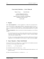
Uncertainty Machine — User’s Manual
Thomas Lafarge
Antonio Possolo
Statistical Engineering Division
Information Technology Laboratory
National Institute of Standards and Technology
Gaithersburg, Maryland, USA
July 10, 2013
1
Purpose
NIST’s UncertaintyMachine is a software application to evaluate the measurement uncertainty associated with an output quantity defined by a measurement model of the form y =
f (x 1 , . . . , x n ), where the real-valued function f is specified fully and explicitly, and the input
quantities are modeled as random variables whose joint probability distribution also is specified
fully.
The UncertaintyMachine evaluates measurement uncertainty by application of two different
methods:
• The method introduced by Gauss [1823] and described in the Guide to the Evaluation of
Uncertainty in Measurement (GUM) [Joint Committee for Guides in Metrology, 2008a]
and also by Taylor and Kuyatt [1994];
• The Monte Carlo method described by Morgan and Henrion [1992] and specified in the
Supplement 1 to the GUM (GUM-S1) [Joint Committee for Guides in Metrology, 2008b].
2
Gauss’s Formula vs. Monte Carlo Method
The method described in the GUM produces an approximation to the standard measurement
uncertainty u( y) of the output quantity, and it requires:
(a) Estimates x 1 , . . . , x n of the input quantities;
(b) Standard measurement uncertainties u(x 1 ), . . . , u(x n );
(c) Correlations {ri j } between every pair of different input quantities (by default these are all
assumed to be zero);
(d) Values of the partial derivatives of f evaluated at x 1 , . . . , x n .
lafarge & possolo
page 1 of 19
nist
uncertainty machine v. 1.0
When the probability distribution of the output quantity is approximately Gaussian, then the
interval y ± 2u( y) may be interpreted as a coverage interval for the measurand with approximately 95 % coverage probability.
The GUM also considers the case where the distribution of the output quantity is approximately
Student’s t with a number of degrees of freedom that may be a function of the numbers of
degrees of freedom that the {u(x j )} are based on, computed using the Welch-Satterthwaite
formula [Satterthwaite, 1946, Welch, 1947].
In general, neither the Gaussian nor the Student’s t distributions need model the dispersion
of values of the output quantity accurately, even when all the input quantities are modeled as
Gaussian random variables.
The GUM suggests that the Central Limit Theorem (CLT) lends support to the Gaussian approximation for the distribution of the output quantity. However, without a detailed examination of
the measurement function f , and of the probability distribution of the input quantities (examinations that the GUM does not explain how to do), it is impossible to guarantee the adequacy
of the Gaussian or Student’s t approximations.
note. The CLT states that, under some conditions, a sum of independent random variables has a probability distribution that is approximately Gaussian [Billingsley, 1979, Theorem 27.2]. The CLT is a limit theorem, in the sense that it concerns an infinite sequence
of sums, and provides no indication about how close to Gaussian the distribution of a sum
of a finite number of summands will be. Other results in probability theory provide such
indications, but they involve more than just the means and variances that are required to
apply Gauss’s formula.
The Monte Carlo method provides an arbitrarily large sample from the probability distribution
of the output quantity, and it requires that the joint probability distribution of the random
variables modeling the input quantities be specified fully.
This sample alone suffices to compute the standard uncertainty associated with the output
quantity, and to compute and to interpret coverage intervals probabilistically.
example. Suppose that the measurement model is y = ab/c, and that a, b, and c are
modeled as independent random variables such that:
• a is Gaussian with mean 32 and standard deviation 0.5;
• b has a uniform (or, rectangular) distribution with mean 0.9 and standard deviation
0.025;
• c has a symmetrical triangular distribution with mean 1 and standard deviation 0.3.
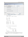
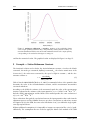
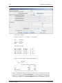
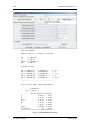
Figure 1 on Page 3 shows the graphical user interface of the UncertaintyMachine filled in
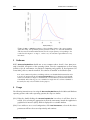
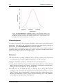
to reflect these modeling choices, and the results that are printed on-screen. Figure 2 on
Page 4 shows a probability density estimate of the distribution of the output quantity.
The method described in the GUM produces y = 28.8 and u( y) = 8.7. According to
the conventional interpretation, the interval (11.4, 46.2) may be a coverage interval with
approximately 95 % coverage probability.
A sample of size 1 × 107 produced by application of the Monte Carlo method has average 32.20 and standard deviation 12.53. Since only 88 % of the sample values lie within
(11.4, 46.2), the coverage probability of this coverage interval is much lower than the conventional interpretation would have led one to believe.
lafarge & possolo
page 2 of 19
nist
uncertainty machine v. 1.0
Monte Carlo Method
Summary statistics for sample of size 1e+06
ave
sd
median
mad
=
=
=
=
32.2
12.5
28.8
8.9
Coverage intervals
99%
95%
90%
68%
50%
(
(
(
(
(
17.12 ,
18 ,
19.11 ,
21.8 ,
23.7 ,
85
67
58
42
37
)
)
)
)
)
k
k
k
k
k
=
=
=
=
=
2.7
2
1.6
0.81
0.53
-------------------------------------------Gauss’s Formula (GUM’s Linear Approximation)
y
= 28.8
u(y) = 8.69
SensitivityCoeffs Percent.u2
a
0.9
0.27
b
32.0
0.85
c
-29.0
99.00
Correlations
NA
0.00
============================================
Figure 1: ABC. Entries in the GUI correspond to the example discussed in §2. In each
numerical result, only the digits that the UncertaintyMachine deems to be significant
are printed.
lafarge & possolo
page 3 of 19
nist
uncertainty machine v. 1.0
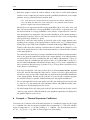
Figure 2: ABC — Densities. Estimate of the probability density of the output quantity
(solid blue line), and probability density (dotted red line) of a Gaussian distribution
with the same mean and standard deviation as the output quantity, corresponding to the
results listed in Figure 1 on Page 3. In this case, the Gaussian approximation is very
inaccurate.
3
Software
NIST’s UncertaintyMachine should run on any computer where Oracle’s Java (www.java.
com) is installed, irrespective of the operating system. Since the computations are done using
facilities of the R environment for statistical computing and graphics [R Development Core
Team, 2012], this too, must be installed. The software is installed as described in §10.
note. Some commercial products, including software, are identified in this manual in order
to specify the means whereby the UncertaintyMachine may be employed. Such identification is not intended to imply recommendation or endorsement by the National Institute
of Standards and Technology, nor is it intended to imply that the software identified is
necessarily the only or best available for the purpose.
4
Usage
The following instructions are for using the UncertaintyMachine under the Microsoft Windows
operating system: under other operating systems, the steps are similar.
(U-1) Either by double-clicking the UncertaintyMachine icon where it will have been installed, or by selecting the appropriate item in the Start menu, launch the application’s
graphical user interface (GUI), which is displayed in a resizable window.
(U-2) If one wishes to use a saved configuration, click Load Parameters, select the file where
parameters will have been saved previously, and continue.
lafarge & possolo
page 4 of 19
nist
uncertainty machine v. 1.0
(U-3) Choose the number of input quantities from the drop-down menu corresponding to the
entry Number of input quantities. In response to this, the GUI will update itself and
show as many boxes as there are input quantities, and assign default names to them
(which may be changed as explained below).
(U-4) Enter the size of the sample to be drawn from the probability distribution of the output
quantity, into the box labeled Number of realizations of output quantity: the default value, 1 × 106 , is the minimum recommended sample size.
(U-5) Enter the names of the input quantities into the boxes following Names of input quantities.
(U-6) Click the button labeled Update quantity names: this will update the labels of the
boxes that appear farther down in the GUI that are used to assign probability distributions to the input quantities.
(U-7) Enter a valid R expression into the box labeled Value of output quantity (R expression)
that defines the value of the output quantity. This expression should involve only the input quantities, and functions and numerical constants that R knows how to evaluate.
(Remember that R is case sensitive.)
Alternatively, the definition may comprise several R expressions, possibly in different
lines within this box (pressing Enter on the keyboard, with the cursor in this box, creates
a new line), but the last expression must evaluate the output quantity (without assigning
this value to any variable).
example. If the measurement model is A = (L1 − L0 )/ L0 (T1 − T0 ) , then the R
expression that should then be entered into this box is (L1-L0)/(L0*(T1-T0)).
Alternatively, the box may comprise these three lines:
N = L1-L0
D = L0*(T1-T0)
N / D
Note that the last expression produces the value f (x 1 , . . . , x n ) that the measurement
function takes at the estimates of the input quantities.
(U-8) Assign a probability distribution to each of the input quantities, using the drop-down
menus in front of them. Once a choice is made, one or more additional input boxes
will appear, where values of parameters must be entered fully to specify the probability
distribution that was selected. Table 1 on Page 7 lists the distributions implemented
currently, and their parametrizations. Note that some distributions have more than one
parametrization: in such cases, only one of the parametrizations needs to be specified.
(U-9) If there are correlations between input quantities that need to be taken into account,
then check the box marked Correlations, and enter the values of non-zero correlations
into the appropriate boxes in the upper triangle of the correlation matrix that the GUI
will display.
(U-10) If the box marked Correlations has been checked, then besides having specified correlations in (U-9), also select a copula (currently, either Gaussian or Student’s t) to
manufacture a joint probability distribution for the input quantities. If the copula chosen
is (multivariate) Student’s t, then another box will appear nearby to receive the number
of degrees of freedom.
lafarge & possolo
page 5 of 19
nist
uncertainty machine v. 1.0
note. The resulting joint distribution reproduces the correlation structure that has
been specified, and has the distributions specified for the input quantities as margins. Possolo [2010] explains and illustrates the role that copulas play in uncertainty
analysis.
(U-11) Optionally, if you wish to save the results of the calculations (numerical and graphical), then click the button labeled Choose file, and use the file selection dialog that is
displayed to select the location, and the prefix for the output files.
The prefix will be used to define the names of the three output files that will be created:
(i) a plain ASCII text file where the sample of values of the output quantity will be
written to, one per line; (ii) a JPEG file with a plot; and (iii) a plain ASCII text file with
summary statistics of the Monte Carlo sample drawn from the distribution of the output
quantity, and with the estimate of the measurand and the standard uncertainty evaluated
as specified in the GUM.
example. If the specified prefix is ABC.txt or ABC, then the three output files that
will be created and named automatically will be called ABC-values.txt, ABC-density.jpg
and ABC-results.txt.
(U-12) Optionally, save the parameters specified in the GUI by clicking Save Parameters and
choosing a file to save the GUI’s current configuration to. This configuration comprises
the definition of the measurement model and the parameter settings.
(U-13) Click the button labeled Run. In response to this, a window will open where numerical
results will be printed, and a graphics window will also open to display graphical results.
If a file name will have been specified in (U-11), then both numerical and graphical
output are saved to files.
The UncertaintyMachine estimates the number of significant digits in the results, and
reports only these. To increase the number of significant digits, another run will have to
be done with a larger sample size than what was specified in (U-4).
(U-14) To quit, press the button labeled Quit on the GUI, and close the window that the
UncertaintyMachine created in (U-13), which will induce the graphics window also
to close.
5
Results
The UncertaintyMachine produces output in two windows on the screen, and optionally writes
three files to disk, described next.
• One of the outputs shown on the computer screen is an R graphics window that shows
a kernel estimate [Silverman, 1986] of the probability density of the output quantity
(drawn in a solid blue line), and the probability density of the Gaussian distribution with
the same mean and standard deviation as the Monte Carlo sample of values of the output
quantity (drawn as a red dotted line).
lafarge & possolo
page 6 of 19
nist
uncertainty machine v. 1.0
name
parameters
constraints
Bernoulli
Beta
Prob. of success
Mean, StdDev
Shape1, Shape2
DF
Mean
Mean, StdDev
Shape, Scale
Mean, StdDev
Mean, StdDev, Left, Right
Mean, StdDev
Left, Right
Mean, StdDev, DF
Center, Scale, DF
Mean, StdDev
Left, Right
Left, Right, Mode
Mean, StdDev
Left, Right
Mean, StdDev
Shape, Scale
0 < Prob. of success < 1
0 < Mean < 1, 0 < StdDev < ½
Shape1 > 0, Shape2 > 0
DF > 0
Mean > 0
Mean > 0, StdDev > 0
Shape > 0, Scale > 0
StdDev > 0
StdDev > 0, Left < Right
StdDev > 0
Left < Right
StdDev > 0, DF > 2
Scale > 0, DF > 0
StdDev > 0
Left < Right
Left ¶ Mode ¶ Right; Left 6= Right
StdDev > 0
Left < Right
Mean > 0, StdDev > 0
Shape > 0, Scale > 0
Chi-Squared
Exponential
Gamma
Gaussian
Gaussian – Truncated
Rectangular
Student’s t
Triangular – Symmetric
Triangular – Asymmetric
Uniform
Weibull
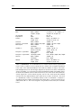
Table 1: Distributions. Several distributions are available with alternative parametrizations: for these, it suffices to select and specify one of them. The rectangular distribution
is the same as the uniform distribution. DF stands for number of degrees of freedom.
Left and Right denote the left and right endpoints of the interval to which a distribution
assigns probability 1. For the truncated Gaussian distribution, Mean and StdDev denote
the mean and standard deviation without truncation: the actual mean and standard deviation depend also on the truncation points, and it is the actual mean and standard
deviation that the GUM and Monte Carlo methods use in their calculations. The mode
of a distribution is where its probability density reaches its maximum. A Student’s t
distribution will have infinite standard deviation unless DF > 2, and its mean will be undefined unless DF > 1. The values assigned to the parameters must satisfy the constraints
listed.
lafarge & possolo
page 7 of 19
nist
uncertainty machine v. 1.0
• Numerical output is written in another window, in the form of a table with summary
statistics for the sample that was drawn from the probability distribution of the output
quantity: average, standard deviation, median, mad.
note. “mad” denotes the median absolute deviation from the median, multiplied by
a factor (1.4826) that makes the result comparable to the standard deviation when
applied to samples from Gaussian distributions.
Also listed are coverage intervals with coverage probabilities 99 %, 95 %, 90 %, 68 %, and
50 %. The interval with 68 % coverage probability is often called a “1-sigma interval”, and
the interval with 95 % coverage probability is often called a “2-sigma interval”: however,
these designations are appropriate only when the distribution of the output quantity is
approximately Gaussian. Next to each interval is listed the value of the corresponding
coverage factor k (cf. GUM §3.3.7, §6.2).
Below these, and in the same window, are listed the value of the output quantity corresponding to the estimates of the input quantities, and the value of u( y) computed using
formula (13) in the GUM [Joint Committee for Guides in Metrology, 2008a, Page 21].
Finally, a table shows the sensitivity coefficients that are defined in the GUM §5.1.3: the
values of the partial derivatives of the measurement function f evaluated at the estimates
of the input quantities.
The same table also shows the percentage contributions that the different input quantities
make to the squared standard uncertainty of the output quantity. If the input quantities
are uncorrelated, then these contributions add up to 100 % approximately. If they are
correlated, then the contributions may add up to more or less than 100 %: in this case,
the line labeled Correlations will indicate the percentage of u2 ( y) that is attributable to
those correlations (this percentage is positive if u2 ( y) is larger than it would have been
in the absence of correlations).
• If the user has specified a file name prefix in (U-11), following Save results in file
in the GUI, then the first output file name ends in -values.txt and is a plain ASCII text
file with one value per line of the sample that was drawn from the probability distribution
of the output quantity. This file may be read into R or into any other computer program
for statistical analysis, to produce additional numerical and graphical summaries.
• The second output file has the same prefix as the file just mentioned, but its name ends
in -results.txt, and contains the same summary statistics and GUM uncertainty evaluation that were already displayed on the screen.
• The third output file has the same prefix as the file just mentioned, but its name ends in
-density.jpg, and it is a JPEG file with the same graphical output that was displayed in
the graphics window on the screen.
6
Example — Thermal Expansion Coefficient
To measure the coefficient of linear thermal expansion of a cylindrical copper bar, the length
L0 = 1.4999 m of the bar was measured with the bar at temperature T0 = 288.15 K, and then
again at temperature T1 = 373.10 K, yielding L1 = 1.5021 m. The measurement model is
A = (L1 − L0 )/ L0 (T1 − T0 ) (this “A” denotes uppercase Greek alpha).
lafarge & possolo
page 8 of 19
nist
uncertainty machine v. 1.0
For the purpose of this illustration we will assume that the input quantities are like (scaled
and shifted) Student’s t random variables with 3 degrees of freedom, with means equal to
the measured values given, and standard deviations u(L0 ) = 0.0001 m, u(L1 ) = 0.0002 m,
u(T0 ) = 0.02 K, and u(T1 ) = 0.05 K.
note. The assignment of distributions to the four input quantities would be appropriate if
their estimates were averages of four replicated readings each, and these were outcomes
of independent Gaussian random variables with unknown common mean and standard
deviation.
The GUM’s approach yields α = 1.727 × 10−5 K−1 and u(α) = 1.8 × 10−6 K−1 , and the Monte
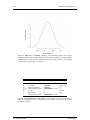
Carlo method reproduces these results. Figure 3 on Page 10 reflects these facts, and lists the
numerical results. The graphical results are displayed in Figure 4 on Page 11.
7
Example — End-Gauge Calibration
In Example H.1 of the GUM (which is reconsidered by Guthrie et al. [2009]), the measurement
model is l = lS + d − lS (δα · θ + αS · δθ ). The estimates and standard measurement uncertainties of the input quantities are listed in Table 2. For the Monte Carlo method, we model
the input quantities as independent Gaussian random variables with means and standard deviations equal to these estimates and standard measurement uncertainties.
quantity
x
u(x)
lS
d
δα
θ
αS
δθ
50 000 623 nm
215 nm
0 ◦C−1
−0.1 ◦C
11.5 × 10−6 ◦C−1
0 ◦C
25 nm
9.7 nm
0.58 × 10−6 ◦C−1
0.41 ◦C
1.2 × 10−6 ◦C−1
0.029 ◦C
Table 2: End-Gauge Calibration. Estimates and standard measurement uncertainties
for the input quantities in the measurement model of Example H.1 in the GUM.
The GUM’s approach yields l = 50 000 838 nm and u(l) = 32 nm, while the Monte Carlo method
reproduces the value for l but evaluates u(l) = 34 nm.
The GUM (Page 84) gives (50 000 745 nm, 50 000 931 nm) as an approximate 99 % coverage
interval for l, and the results of the Monte Carlo method confirm this coverage probability. If
one chooses a coverage interval that is probabilistically symmetric (meaning that it leaves 0.5 %
of the Monte Carlo sample uncovered on both sides), then the Monte Carlo method produces
(50 000 749 nm, 50 000 927 nm) as 99 % coverage interval (and this is not quite centered at the
estimate of y).
Figure 5 on Page12 reflects these facts and lists the numerical results. The graphical results are
displayed in Figure 6 on Page 13.
lafarge & possolo
page 9 of 19
nist
uncertainty machine v. 1.0
Monte Carlo Method
Summary statistics for sample of size 1e+06
ave
sd
median
mad
=
=
=
=
1.727e-05
1.7e-06
1.727e-05
1e-06
Coverage intervals
99%
95%
90%
68%
50%
(
(
(
(
(
1.15e-05 ,
1.4e-05 ,
1.48e-05 ,
1.6e-05 ,
1.643e-05 ,
2.3e-05 )
2.05e-05 )
1.973e-05 )
1.857e-05 )
1.811e-05 )
k
k
k
k
k
=
=
=
=
=
3.3
1.9
1.4
0.74
0.48
-------------------------------------------Gauss’s Formula (GUM’s Linear Approximation)
y
= 1.727e-05
u(y) = 1.8e-06
SensitivityCoeffs Percent.u2
L0
-7.9e-03
2.0e+01
L1
7.8e-03
8.0e+01
T0
2.0e-07
5.4e-04
T1
-2.0e-07
3.4e-03
Correlations
NA
0.0e+00
## ============================================
Figure 3:
Thermal Expansion Coefficient. Entries in the GUI correspond to
the example discussed in §6. In each numerical result, only the digits that the
UncertaintyMachine deems to be significant are printed.
lafarge & possolo
page 10 of 19
nist
uncertainty machine v. 1.0
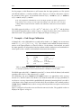
Figure 4: Thermal Expansion Coefficient — Densities. Estimate of the probability
density of the output quantity (solid blue line), and probability density (dotted red line)
of a Gaussian distribution with the same mean and standard deviation as the output
quantity, corresponding to the results listed in Figure 3 on Page 10.
8
Example — Resistance
In Example H.2 of the GUM, the measurement model for the resistance of an element of an
electrical circuit is R = (V /I) cos(φ). The estimates and standard uncertainties of the input
quantities, and the correlations between them, are listed in Table 3 on Page 11.
For the Monte Carlo method, we model the input quantities as correlated Gaussian random
variables with means and standard deviations equal to the estimates and standard uncertainties
listed in Table 3, and with correlations identical to those given in the same table. We also
adopt a Gaussian copula to manufacture a joint probability distribution consistent with the
assumptions already listed.
quantity
x
u(x)
V
I
φ
4.9990 V
19.6610 × 10−3 A
1.044 46 rad
0.0032 V
0.0095 × 10−3 A
0.000 75 rad
r(V, I) = −0.36
r(V, φ) = 0.86
r(I, φ) = −0.65
Table 3: Resistance. Estimates and standard measurement uncertainties for the input quantities in the measurement model of Example H.2 in the GUM, and correlations
between them, all as listed in Table H.2 of the GUM.
The GUM’s approach and the Monte Carlo method produce the same values of the output
quantity R = 127.732 Ω and of the standard uncertainty u(R) = 0.07 Ω. The Monte Carlo
method yields (127.595 Ω, 127.869 Ω) as approximate 95 % coverage interval for the resistance
without invoking any additional assumptions about R. Figure 7 on Page 14 reflects these facts,
lafarge & possolo
page 11 of 19
nist
uncertainty machine v. 1.0
Monte Carlo Method
Summary statistics for sample of size 1e+06
ave
sd
median
mad
=
=
=
=
50000838
33.9
50000838
34
Coverage intervals
99%
95%
90%
68%
50%
(
(
(
(
(
50000750
50000770
50000780
50000804
50000815
,
,
,
,
,
50000927
50000900
50000894
50000872
50000861
)
)
)
)
)
k
k
k
k
k
=
=
=
=
=
2.6
1.9
1.7
1
0.68
-------------------------------------------Gauss’s Formula (GUM’s Linear Approximation)
y
= 50000838
u(y) = 31.7
SensitivityCoeffs Percent.u2
lS
1
62.00
d
1
9.40
dalpha
5000000
0.84
theta
0
0.00
alphaS
0
0.00
dtheta
-580
28.00
Correlations
NA
0.00
============================================
Figure 5: End-Gauge Calibration.
lafarge & possolo
page 12 of 19
nist
uncertainty machine v. 1.0
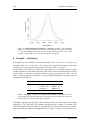
Figure 6: End-Gauge Calibration — Densities. Estimate of the probability density
of the output quantity (solid blue line), and probability density (dotted red line) of a
Gaussian distribution with the same mean and standard deviation as the output quantity,
corresponding to the results listed in Figure 5 on Page 12.
and lists the numerical results. The graphical results are displayed in Figure 8 on Page 15.
9
Example — Stefan-Boltzmann Constant
The functional relation used to define the Stefan-Boltzmann constant σ involves the Planck
constant h, the molar gas constant R, Rydberg’s constant R∞ , the relative atomic mass of the
electron Ar (e), the molar mass constant Mu , the speed of light in vacuum c, and the finestructure constant α:
32π5 hR4 R4∞
σ=
.
(1)
15Ar (e)4 Mu4 c 6 α8
Table 4 lists the 2010 CODATA [Mohr et al., 2012] recommended values of the quantities that
determine the value of the Stefan-Boltzmann constant, and the measurement uncertainties
associated with them.
According to the GUM, the estimate of the measurand equals the value of the measurement
function evaluated at the estimates of the input quantities, as σ = 5.670 37 × 10−8 W m−2 K−4 .
Both the GUM’s approximation and the Monte Carlo method produce the same evaluation of
u(σ) = 2 × 10−13 W m−2 K−4 .
These evaluations disregard the correlations between the input quantities that result from the
adjustment process used by CODATA. However, once these correlations are taken into account
via Equation (13) in the GUM, the same value still obtains for u(σ) to within the single significant digit reported above.
Without additional assumptions, it is impossible to interpret an expression like σ ± u(σ) probabilistically. The assumptions that are needed to apply the Monte Carlo method of the GUM
lafarge & possolo
page 13 of 19
nist
uncertainty machine v. 1.0
Monte Carlo Method
Summary statistics for sample of size 1e+06
ave
sd
median
mad
=
=
=
=
127.732
0.07
127.732
0.07
Coverage intervals
99%
95%
90%
68%
50%
(
(
(
(
(
127.55 ,
127.595 ,
127.617 ,
127.662 ,
127.685 ,
127.912 )
127.8689 )
127.847 )
127.802 )
127.779 )
k
k
k
k
k
=
=
=
=
=
2.6
2
1.6
1
0.67
-------------------------------------------Gauss’s Formula (GUM’s Linear Approximation)
y
= 127.732
u(y) = 0.07
SensitivityCoeffs Percent.u2
V
26
140
I
-6500
78
phi
-220
560
Correlations
NA
-670
============================================
Figure 7: Resistance. Entries in the GUI correspond to the example discussed in §8.
Note that, in this case, the UncertaintyMachine reconfigured its graphical user automatically to accommodate the correlations that had to be specified. In each numerical
result, only the digits that the UncertaintyMachine deems to be significant are printed.
lafarge & possolo
page 14 of 19
nist
uncertainty machine v. 1.0
Figure 8: Resistance — Densities. Estimate of the probability density of the output
quantity (solid blue line), and probability density (dotted red line) of a Gaussian distribution with the same mean and standard deviation as the output quantity, corresponding
to the results listed in Figure 7 on Page 14.
h
R
R∞
Ar (e)
Mu
c
α
value
std. meas. unc.
unit
6.626 069 57 × 10−34
8.314 462 1
10 973 731.568 539
5.485 799 094 6 × 10−4
1 × 10−3
299 792 458
7.297 352 569 8 × 10−3
0.000 000 29 × 10−34
0.000 007 5
0.000 055
0.000 000 002 2 × 10−4
0
0
0.000 000 002 4 × 10−3
Js
J mol−1 K−1
m−1
u
kg/mol
m/s
1
Table 4: Stefan-Boltzmann. 2010 CODATA recommended values and standard measurement uncertainties for the quantities used to define the value of the StefanBoltzmann constant.
lafarge & possolo
page 15 of 19
nist
uncertainty machine v. 1.0
Supplement 1 deliver not only an evaluation of uncertainty, but also enable a probabilistic
interpretation.
If the measurement uncertainties associated with h, R, R∞ , Ar (e), and α are expressed by
modeling these quantities as independent Gaussian random variables with means and standard
deviations set equal to the values and standard measurement uncertainties listed in Table 4,
then the distribution that the Monte Carlo method of the GUM Supplement 1 assigns to the
measurand happens to be approximately Gaussian as gauged by the Anderson-Darling test of
Gaussian shape [Anderson and Darling, 1952].
Figure 9 on Page 17 reflects these facts and lists the numerical results, which imply that the
interval from 5.670 332 × 10−8 W m−2 K−4 to 5.670 412 6 × 10−8 W m−2 K−4 is a coverage interval for σ with approximate 95 % coverage probability. The probability density of σ, and the
corresponding Gaussian approximation are displayed in Figure 10 on Page 18.
10
Software Installation
If R has not been previously installed in the target machine, then it will have to be installed first.
R is free and open-source, with versions available for all major operating systems: it may be
downloaded from www.r-project.org. A Java Runtime Environment (JRE) is also necessary:
it may be downloaded from www.java.com.
10.1
Microsoft Windows
Open the distribution ZIP archive, which contains the installer and the user’s manual, and
execute the installer. During installation, a dialog box will prompt the user to select whether
(the default is to do them all):
• Rscript.exe should be added to the search path for executables;
• Missing R packages should be installed automatically;
• A desktop icon should be created.
10.2
Linux
Assuming that R (version 2.14 or newer), a JRE, and xterm are installed on the system and
are in the user’s PATH for executables, then installation amounts to extracting the contents of
the distribution archive, and placing them in the desired folder, then executing the command
Rscript configure-R.R to install the required R packages. The software can be started by executing either the command java -jar UncertaintyMachine.jar or the shell script run.sh.
10.3
Apple OS X
The installation under Apple OS X is similar to the installation under Linux, including the
requirement that xterm be installed: it is different from the Terminal application, and it is part
of Apple’s X11 package. Under Mountain Lion, X11 installs on demand: when an application
is first launched that requires X11 libraries, the user is directed to a download location for the
most up-to-date version of X11 for the Mac.
lafarge & possolo
page 16 of 19
nist
uncertainty machine v. 1.0
Monte Carlo Method
Summary statistics for sample of size 1e+06
ave
sd
median
mad
=
=
=
=
5.67037e-08
2.05e-13
5.6703725e-08
2.05e-13
Coverage intervals
99%
95%
90%
68%
50%
(
(
(
(
(
5.67032e-08 ,
5.670332e-08 ,
5.670339e-08 ,
5.6703521e-08 ,
5.670359e-08 ,
5.670425e-08 )
5.6704126e-08 )
5.6704062e-08 )
5.670393e-08 )
5.670386e-08 )
k
k
k
k
k
=
=
=
=
=
2.6
2
1.6
1
0.66
-------------------------------------------Gauss’s Formula (GUM’s Linear Approximation)
y
= 5.67037e-08
u(y) = 2.05e-13
SensitivityCoeffs Percent.u2
h
8.6e+25
1.5e-02
R
2.7e-08
1.0e+02
Rinfty
2.1e-14
3.1e-09
Ae
-4.1e-04
2.0e-05
Mu
-2.3e-04
0.0e+00
c
-1.1e-15
0.0e+00
alpha
-6.2e-05
5.3e-05
Correlations
NA
0.0e+00
============================================
Figure 9: Stefan Boltzmann constant.
lafarge & possolo
page 17 of 19
nist
uncertainty machine v. 1.0
Figure 10: Stefan-Boltzmann — Densities. Estimate of the probability density of the
output quantity (solid blue line), and probability density (dotted red line) of a Gaussian
distribution with the same mean and standard deviation as the output quantity, corresponding to the results listed in Figure 9 on Page 17.
Acknowledgments
The authors are grateful to their colleagues Will Guthrie, Alan Heckert, Narain Krishnamurthy,
Adam Pintar, Jolene Splett, and Jack Wang, for the many suggestions that they offered for
improvement of the UncertaintyMachine and of this user’s manual.
The authors will be very grateful to users of the software, and to readers of this manual, for
information about errors and other deficiencies, and for suggestions for improvement, which
may be sent via eMail to [email protected].
References
T. W. Anderson and D. A. Darling. Asymptotic theory of certain “goodness-of-fit” criteria based
on stochastic processes. Annals of Mathematical Statistics, 23:193–212, 1952.
P. Billingsley. Probability and Measure. John Wiley & Sons, New York, NY, 1979.
C. Gauss. Theoria combinationis observationum erroribus minimis obnoxiae. In Werke, Band IV,
Wahrscheinlichkeitsrechnung und Geometrie. Könighlichen Gesellschaft der Wissenschaften,
Göttingen, 1823. http://gdz.sub.uni-goettingen.de/.
W. F. Guthrie, H.-k. Liu, A. L. Rukhin, B. Toman, J. C.M. Wang, and N.-f. Zhang. Three statistical
paradigms for the assessment and interpretation of measurement uncertainty. In F. Pavese
and A. B. Forbes, editors, Data Modeling for Metrology and Testing in Measurement Science,
Modeling and Simulation in Science, Engineering and Technology, pages 1–45. Birkhäuser
Boston, 2009. doi: 10.1007/978-0-8176-4804-6_3.
lafarge & possolo
page 18 of 19
nist
uncertainty machine v. 1.0
Joint Committee for Guides in Metrology. Evaluation of measurement data — Guide to the
expression of uncertainty in measurement. International Bureau of Weights and Measures
(BIPM), Sèvres, France, September 2008a. URL http://www.bipm.org/en/publications/
guides/gum.html. BIPM, IEC, IFCC, ILAC, ISO, IUPAC, IUPAP and OIML, JCGM 100:2008,
GUM 1995 with minor corrections.
Joint Committee for Guides in Metrology. Evaluation of measurement data — Supplement 1
to the “Guide to the expression of uncertainty in measurement” — Propagation of distributions
using a Monte Carlo method. International Bureau of Weights and Measures (BIPM), Sèvres,
France, 2008b. URL http://www.bipm.org/en/publications/guides/gum.html. BIPM,
IEC, IFCC, ILAC, ISO, IUPAC, IUPAP and OIML, JCGM 101:2008.
P. J. Mohr, B. N. Taylor, and D. B. Newell. CODATA recommended values of the fundamental
physical constants: 2010. Reviews of Modern Physics, 84(4):1527–1605, October-December
2012.
M. G. Morgan and M. Henrion. Uncertainty — A Guide to Dealing with Uncertainty in Quantitative Risk and Policy Analysis. Cambridge University Press, New York, NY, first paperback
edition, 1992. 10th printing, 2007.
A. Possolo. Copulas for uncertainty analysis. Metrologia, 47:262–271, 2010.
R Development Core Team. R: A Language and Environment for Statistical Computing. R Foundation for Statistical Computing, Vienna, Austria, 2012. URL http://www.R-project.org.
ISBN 3-900051-07-0.
F. E. Satterthwaite. An approximate distribution of estimates of variance components. Biometrics
Bulletin, 2(6):110–114, December 1946.
B. W. Silverman. Density Estimation. Chapman and Hall, London, 1986.
B. N. Taylor and C. E. Kuyatt. Guidelines for Evaluating and Expressing the Uncertainty of NIST
Measurement Results. National Institute of Standards and Technology, Gaithersburg, MD,
1994. URL http://physics.nist.gov/Pubs/guidelines/TN1297/tn1297s.pdf. NIST
Technical Note 1297.
B. L. Welch. The generalization of ‘Student’s’ problem when several different population variances are involved. Biometrika, 34:28–35, January 1947.
lafarge & possolo
page 19 of 19