Download FFT MegaCore Function User Guide

FFT MegaCore Function User Guide
FFT MegaCore Function
User Guide
101 Innovation Drive
San Jose, CA 95134
www.altera.com
UG-FFT-12.0
Feedback Subscribe
© 2012 Altera Corporation. All rights reserved. ALTERA, ARRIA, CYCLONE, HARDCOPY, MAX, MEGACORE, NIOS, QUARTUS and STRATIX words and logos
are trademarks of Altera Corporation and registered in the U.S. Patent and Trademark Office and in other countries. All other words and logos identified as
trademarks or service marks are the property of their respective holders as described at www.altera.com/common/legal.html. Altera warrants performance of its
semiconductor products to current specifications in accordance with Altera's standard warranty, but reserves the right to make changes to any products and
services at any time without notice. Altera assumes no responsibility or liability arising out of the application or use of any information, product, or service
described herein except as expressly agreed to in writing by Altera. Altera customers are advised to obtain the latest version of device specifications before relying
on any published information and before placing orders for products or services.
November 2012
Altera Corporation
ISO
9001:2008
Registered
FFT MegaCore Function
User Guide
Contents
Chapter 1. About This MegaCore Function
Release Information . . . . . . . . . . . . . . . . . . . . . . . . . . . . . . . . . . . . . . . . . . . . . . . . . . . . . . . . . . . . . . . . . . . . . 1–1
Device Family Support . . . . . . . . . . . . . . . . . . . . . . . . . . . . . . . . . . . . . . . . . . . . . . . . . . . . . . . . . . . . . . . . . . . 1–1
Features . . . . . . . . . . . . . . . . . . . . . . . . . . . . . . . . . . . . . . . . . . . . . . . . . . . . . . . . . . . . . . . . . . . . . . . . . . . . . . . . 1–2
General Description . . . . . . . . . . . . . . . . . . . . . . . . . . . . . . . . . . . . . . . . . . . . . . . . . . . . . . . . . . . . . . . . . . . . . 1–3
Fixed Transform Size Architecture . . . . . . . . . . . . . . . . . . . . . . . . . . . . . . . . . . . . . . . . . . . . . . . . . . . . . . 1–3
Variable Streaming Architecture . . . . . . . . . . . . . . . . . . . . . . . . . . . . . . . . . . . . . . . . . . . . . . . . . . . . . . . . 1–4
MegaCore Verification . . . . . . . . . . . . . . . . . . . . . . . . . . . . . . . . . . . . . . . . . . . . . . . . . . . . . . . . . . . . . . . . . . . 1–4
Performance and Resource Utilization . . . . . . . . . . . . . . . . . . . . . . . . . . . . . . . . . . . . . . . . . . . . . . . . . . . . . . 1–4
Cyclone III Devices . . . . . . . . . . . . . . . . . . . . . . . . . . . . . . . . . . . . . . . . . . . . . . . . . . . . . . . . . . . . . . . . . . . . 1–5
Stratix III Devices . . . . . . . . . . . . . . . . . . . . . . . . . . . . . . . . . . . . . . . . . . . . . . . . . . . . . . . . . . . . . . . . . . . . . 1–8
Stratix IV Devices . . . . . . . . . . . . . . . . . . . . . . . . . . . . . . . . . . . . . . . . . . . . . . . . . . . . . . . . . . . . . . . . . . . . 1–11
Stratix V Devices . . . . . . . . . . . . . . . . . . . . . . . . . . . . . . . . . . . . . . . . . . . . . . . . . . . . . . . . . . . . . . . . . . . . . 1–14
Installation and Licensing . . . . . . . . . . . . . . . . . . . . . . . . . . . . . . . . . . . . . . . . . . . . . . . . . . . . . . . . . . . . . . . 1–18
OpenCore Plus Evaluation . . . . . . . . . . . . . . . . . . . . . . . . . . . . . . . . . . . . . . . . . . . . . . . . . . . . . . . . . . . . 1–18
OpenCore Plus Time-Out Behavior . . . . . . . . . . . . . . . . . . . . . . . . . . . . . . . . . . . . . . . . . . . . . . . . . . . . . 1–19
Chapter 2. Getting Started
Design Flows . . . . . . . . . . . . . . . . . . . . . . . . . . . . . . . . . . . . . . . . . . . . . . . . . . . . . . . . . . . . . . . . . . . . . . . . . . . 2–1
DSP Builder Flow . . . . . . . . . . . . . . . . . . . . . . . . . . . . . . . . . . . . . . . . . . . . . . . . . . . . . . . . . . . . . . . . . . . . . . . 2–1
MegaWizard Plug-In Manager Flow . . . . . . . . . . . . . . . . . . . . . . . . . . . . . . . . . . . . . . . . . . . . . . . . . . . . . . . 2–2
Parameterize the MegaCore Function . . . . . . . . . . . . . . . . . . . . . . . . . . . . . . . . . . . . . . . . . . . . . . . . . . . . 2–3
Set Up Simulation . . . . . . . . . . . . . . . . . . . . . . . . . . . . . . . . . . . . . . . . . . . . . . . . . . . . . . . . . . . . . . . . . . . . 2–10
Generate the MegaCore Function . . . . . . . . . . . . . . . . . . . . . . . . . . . . . . . . . . . . . . . . . . . . . . . . . . . . . . 2–10
Simulate the Design . . . . . . . . . . . . . . . . . . . . . . . . . . . . . . . . . . . . . . . . . . . . . . . . . . . . . . . . . . . . . . . . . . . . 2–12
Simulate in the MATLAB Software . . . . . . . . . . . . . . . . . . . . . . . . . . . . . . . . . . . . . . . . . . . . . . . . . . . . . 2–13
Fixed Transform Architectures . . . . . . . . . . . . . . . . . . . . . . . . . . . . . . . . . . . . . . . . . . . . . . . . . . . . . . 2–13
Variable Streaming Architecture . . . . . . . . . . . . . . . . . . . . . . . . . . . . . . . . . . . . . . . . . . . . . . . . . . . . . 2–14
Simulate with IP Functional Simulation Models . . . . . . . . . . . . . . . . . . . . . . . . . . . . . . . . . . . . . . . . . . 2–15
Simulating in Third-Party Simulation Tools Using NativeLink . . . . . . . . . . . . . . . . . . . . . . . . . . . . . 2–15
Compile the Design . . . . . . . . . . . . . . . . . . . . . . . . . . . . . . . . . . . . . . . . . . . . . . . . . . . . . . . . . . . . . . . . . . . . . 2–16
Fixed Transform Architecture . . . . . . . . . . . . . . . . . . . . . . . . . . . . . . . . . . . . . . . . . . . . . . . . . . . . . . . . . 2–16
Variable Streaming Architecture . . . . . . . . . . . . . . . . . . . . . . . . . . . . . . . . . . . . . . . . . . . . . . . . . . . . . . . 2–16
Program a Device . . . . . . . . . . . . . . . . . . . . . . . . . . . . . . . . . . . . . . . . . . . . . . . . . . . . . . . . . . . . . . . . . . . . . . 2–16
Chapter 3. Functional Description
Buffered, Burst, & Streaming Architectures . . . . . . . . . . . . . . . . . . . . . . . . . . . . . . . . . . . . . . . . . . . . . . . . . 3–1
Variable Streaming Architecture . . . . . . . . . . . . . . . . . . . . . . . . . . . . . . . . . . . . . . . . . . . . . . . . . . . . . . . . . . . 3–2
The Avalon Streaming Interface . . . . . . . . . . . . . . . . . . . . . . . . . . . . . . . . . . . . . . . . . . . . . . . . . . . . . . . . . . . 3–3
FFT Processor Engine Architectures . . . . . . . . . . . . . . . . . . . . . . . . . . . . . . . . . . . . . . . . . . . . . . . . . . . . . . . . 3–4
Radix-22 Single Delay Feedback Architecture . . . . . . . . . . . . . . . . . . . . . . . . . . . . . . . . . . . . . . . . . . . . . 3–4
Mixed Radix-4/2 Architecture . . . . . . . . . . . . . . . . . . . . . . . . . . . . . . . . . . . . . . . . . . . . . . . . . . . . . . . . . . 3–5
Quad-Output FFT Engine Architecture . . . . . . . . . . . . . . . . . . . . . . . . . . . . . . . . . . . . . . . . . . . . . . . . . . 3–5
Single-Output FFT Engine Architecture . . . . . . . . . . . . . . . . . . . . . . . . . . . . . . . . . . . . . . . . . . . . . . . . . . 3–6
I/O Data Flow Architectures . . . . . . . . . . . . . . . . . . . . . . . . . . . . . . . . . . . . . . . . . . . . . . . . . . . . . . . . . . . . . . 3–6
Streaming . . . . . . . . . . . . . . . . . . . . . . . . . . . . . . . . . . . . . . . . . . . . . . . . . . . . . . . . . . . . . . . . . . . . . . . . . . . . 3–7
Streaming FFT Operation . . . . . . . . . . . . . . . . . . . . . . . . . . . . . . . . . . . . . . . . . . . . . . . . . . . . . . . . . . . . 3–7
Enabling the Streaming FFT . . . . . . . . . . . . . . . . . . . . . . . . . . . . . . . . . . . . . . . . . . . . . . . . . . . . . . . . . . 3–8
November 2012
Altera Corporation
FFT MegaCore Function
User Guide
iv
Contents
Variable Streaming . . . . . . . . . . . . . . . . . . . . . . . . . . . . . . . . . . . . . . . . . . . . . . . . . . . . . . . . . . . . . . . . . . . . 3–8
Change the Block Size . . . . . . . . . . . . . . . . . . . . . . . . . . . . . . . . . . . . . . . . . . . . . . . . . . . . . . . . . . . . . . . 3–8
Enabling the Variable Streaming FFT . . . . . . . . . . . . . . . . . . . . . . . . . . . . . . . . . . . . . . . . . . . . . . . . . . 3–9
Dynamically Changing the FFT Size . . . . . . . . . . . . . . . . . . . . . . . . . . . . . . . . . . . . . . . . . . . . . . . . . . 3–10
The Effect of I/O Order . . . . . . . . . . . . . . . . . . . . . . . . . . . . . . . . . . . . . . . . . . . . . . . . . . . . . . . . . . . . 3–10
Buffered Burst . . . . . . . . . . . . . . . . . . . . . . . . . . . . . . . . . . . . . . . . . . . . . . . . . . . . . . . . . . . . . . . . . . . . . . . 3–11
Burst . . . . . . . . . . . . . . . . . . . . . . . . . . . . . . . . . . . . . . . . . . . . . . . . . . . . . . . . . . . . . . . . . . . . . . . . . . . . . . . 3–13
Parameters . . . . . . . . . . . . . . . . . . . . . . . . . . . . . . . . . . . . . . . . . . . . . . . . . . . . . . . . . . . . . . . . . . . . . . . . . . . . 3–14
Signals . . . . . . . . . . . . . . . . . . . . . . . . . . . . . . . . . . . . . . . . . . . . . . . . . . . . . . . . . . . . . . . . . . . . . . . . . . . . . . . . 3–16
Appendix A. Block Floating Point Scaling
Block Floating Point . . . . . . . . . . . . . . . . . . . . . . . . . . . . . . . . . . . . . . . . . . . . . . . . . . . . . . . . . . . . . . . . . . . .
Calculating Possible Exponent Values . . . . . . . . . . . . . . . . . . . . . . . . . . . . . . . . . . . . . . . . . . . . . . . . . . . . .
Implementing Scaling . . . . . . . . . . . . . . . . . . . . . . . . . . . . . . . . . . . . . . . . . . . . . . . . . . . . . . . . . . . . . . . . . . .
Achieving Unity Gain in an IFFT+FFT Pair . . . . . . . . . . . . . . . . . . . . . . . . . . . . . . . . . . . . . . . . . . . . . . . .
A–1
A–2
A–2
A–4
Additional Information
Revision History . . . . . . . . . . . . . . . . . . . . . . . . . . . . . . . . . . . . . . . . . . . . . . . . . . . . . . . . . . . . . . . . . . . . . Info–1
How to Contact Altera . . . . . . . . . . . . . . . . . . . . . . . . . . . . . . . . . . . . . . . . . . . . . . . . . . . . . . . . . . . . . . . . Info–2
Typographic Conventions . . . . . . . . . . . . . . . . . . . . . . . . . . . . . . . . . . . . . . . . . . . . . . . . . . . . . . . . . . . . . Info–2
FFT MegaCore Function
User Guide
November 2012 Altera Corporation
1. About This MegaCore Function
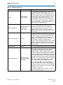
Release Information
Table 1–1 lists information about this release of the Altera® FFT MegaCore® function.
Table 1–1. FFT MegaCore Function Release Information
Item
Version
Release Date
Description
12.1
November 2012
Ordering Code
IP-FFT
Product ID
0034
Vendor ID
6AF7
f For more information about this release, refer to the MegaCore IP Library Release Notes
and Errata.
Altera verifies that the current version of the Quartus® II software compiles the
previous version of each MegaCore® function. The MegaCore IP Library Release Notes
and Errata report any exceptions to this verification. Altera does not verify
compilation with MegaCore function versions older than one release.
Device Family Support
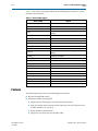
Table 1–2 lists the device support levels for Altera IP cores.
Table 1–2. Altera IP Core Device Support Levels
FPGA Device Families
HardCopy Device Families
Preliminary support—The IP core is verified with
preliminary timing models for this device family. The IP core
meets all functional requirements, but might still be
undergoing timing analysis for the device family. It can be
used in production designs with caution.
HardCopy Companion—The IP core is verified with
preliminary timing models for the HardCopy companion
device. The IP core meets all functional requirements, but
might still be undergoing timing analysis for the HardCopy
device family. It can be used in production designs with
caution.
Final support—The IP core is verified with final timing
models for this device family. The IP core meets all
functional and timing requirements for the device family and
can be used in production designs.
HardCopy Compilation—The IP core is verified with final
timing models for the HardCopy device family. The IP core
meets all functional and timing requirements for the device
family and can be used in production designs.
November 2012
Altera Corporation
FFT MegaCore Function
User Guide
1–2
Chapter 1: About This MegaCore Function
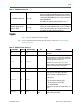
Features
Table 1–3 lists the level of support offered by the FFT MegaCore function to each of
the Altera device families.
Table 1–3. Device Family Support
Device Family
Arria®
Support
GX
Final
Arria II GX
Final
Arria II GZ
Final
Arria V
Refer to the What’s New in Altera IP page of the Altera
website.
Arria V GZ
Preliminary
Cyclone®
Final
Cyclone II
Final
Cyclone III
Final
Cyclone III LS
Final
Cyclone IV
Final
Cyclone V
Refer to the What’s New in Altera IP page of the Altera
website.
HardCopy® II
HardCopy Compilation
HardCopy III
HardCopy Compilation
HardCopy IV E
HardCopy Compilation
HardCopy IV GX
HardCopy Compilation
Stratix®
Final
Stratix II
Final
Stratix II GX
Final
Stratix III
Final
Stratix IV GT
Final
Stratix IV GX/E
Final
Stratix V
Preliminary
Stratix GX
Final
Features
The following lists the features of the FFT MegaCore function:
FFT MegaCore Function
User Guide
■
Bit-accurate MATLAB models
■
Enhanced variable streaming FFT:
■
Single precision floating point or fixed point representation
■
Input and output orders include natural order, bit reversed or digit-reversed,
and DC-centered (–N/2 to N/2)
■
Reduced memory requirements
■
Support for 8 to 32-bit data and twiddle width
November 2012 Altera Corporation
Chapter 1: About This MegaCore Function
General Description
1–3
■
Radix-4, mixed radix-4/2 implementations (for floating point FFT), and radix-22
single delay feedback implementation (for fixed point FFT)
■
Block floating-point architecture—maintains the maximum dynamic range of data
during processing (not for variable streaming)
■
Uses embedded memory
■
Maximum system clock frequency more than 300 MHz
■
Optimized to use Stratix series DSP blocks and TriMatrix™ memory
architecture
■
High throughput quad-output radix 4 FFT engine
■
Support for multiple single-output and quad-output engines in parallel
■
Multiple I/O data flow modes: streaming, buffered burst, and burst
■
User control over optimization in DSP blocks or in speed in Stratix V devices, for
streaming, buffered burst, and burst modes and for variable streaming fixed point
mode
■
Avalon® Streaming (Avalon-ST) compliant input and output interfaces
■
Parameterization-specific VHDL and Verilog HDL testbench generation
■
Transform direction (FFT/IFFT) specifiable on a per-block basis
■
Easy-to-use IP Toolbench interface
■
IP functional simulation models for use in Altera-supported VHDL and Verilog
HDL simulators
■
DSP Builder ready
f For more information about Avalon-ST interfaces, refer to the Avalon Interface
Specifications.
General Description
The FFT MegaCore function is a high performance, highly-parameterizable Fast
Fourier transform (FFT) processor. The FFT MegaCore function implements a
complex FFT or inverse FFT (IFFT) for high-performance applications.
The FFT MegaCore function implements the following architectures:
■
Fixed transform size architecture
■
Variable streaming architecture
Fixed Transform Size Architecture
The fixed transform architecture FFT implements a radix-2/4 decimation-infrequency (DIF) FFT fixed-transform size algorithm for transform lengths of 2m where
6 ≤ m ≤ 16. This architecture uses block-floating point representations to achieve the
best trade-off between maximum signal-to-noise ratio (SNR) and minimum size
requirements.
November 2012
Altera Corporation
FFT MegaCore Function
User Guide
1–4
Chapter 1: About This MegaCore Function
MegaCore Verification
The fixed transform architecture accepts as an input a two’s complement format
complex data vector of length N, where N is the desired transform length in natural
order; the function outputs the transform-domain complex vector in natural order. An
accumulated block exponent is output to indicate any data scaling that has occurred
during the transform to maintain precision and maximize the internal signal-to-noise
ratio. Transform direction is specifiable on a per-block basis via an input port.
Variable Streaming Architecture
The variable streaming architecture FFT implements two different types of
architecture. The variable streaming FFT variations implement either a radix-22 single
delay feedback architecture, using a fixed-point representation, or a mixed radix-4/2
architecture, using a single precision floating point representation. After you select
your architecture type, you can configure your FFT variation during runtime to
perform the FFT algorithm for transform lengths of 2m where 3 ≤ m ≤ 18.
The fixed-point representation grows the data widths naturally from input through to
output thereby maintaining a high SNR at the output. The single precision floating
point representation allows a large dynamic range of values to be represented while
maintaining a high SNR at the output.
f For more information about radix-22 single delay feedback architecture, refer to S. He
and M. Torkelson, A New Approach to Pipeline FFT Processor, Department of Applied
Electronics, Lund University, IPPS 1996.
The order of the input data vector of size N can be natural, bit- or digit-reversed, or
–N/2 to N/2 (DC-centered). The fixed-point representation supports a natural,
bit-reversed, or DC-centered order and the floating point representation supports a
natural, digit-reversed, or DC-centered order. The architecture outputs the
transform-domain complex vector in natural, bit-reversed, or digit-reversed order.
The transform direction is specifiable on a per-block basis using an input port.
MegaCore Verification
Before releasing a version of the FFT MegaCore function, Altera runs comprehensive
regression tests to verify its quality and correctness.
Custom variations of the FFT MegaCore function are generated to exercise its various
parameter options, and the resulting simulation models are thoroughly simulated
with the results verified against master simulation models.
Performance and Resource Utilization
Performance varies depending on the FFT engine architecture and I/O data flow. All
data represents the geometric mean of a three seed Quartus II synthesis sweep.
1
FFT MegaCore Function
User Guide
Cyclone III devices use combinational look-up tables (LUTs) and logic registers;
Stratix III devices use combinational adaptive look-up tables (ALUTs) and logic
registers.
November 2012 Altera Corporation
Chapter 1: About This MegaCore Function
Performance and Resource Utilization
1–5
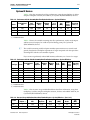
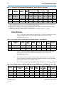
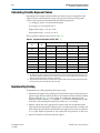
Cyclone III Devices
Table 1–4 lists the streaming data flow performance, using the 4 multipliers/2 adders
complex multiplier structure, for width 16, for Cyclone III (EP3C10F256C6) devices.
Table 1–4. Performance with the Streaming Data Flow Engine Architecture—Cyclone III Devices
Combinational
LUTs
Points
Logic
Registers
Memory
(Bits)
Memory
(M9K)
9×9
Blocks
Clock
Cycle
Count
fMAX
(MHz)
Transform
Time (μs)
256
3437
3906
39168
20
24
231
256
1.11
1024
3857
4650
155904
20
24
244
1024
4.19
3719
4734
622848
76
24
234
4096
17.52
4096
(1)
Note to Table 1–4:
(1) EP3C40F780C6 device.
Table 1–5 shows the variable streaming data flow performance, with in order inputs
and bit-reversed outputs, for width 16 (32 for floating point), for Cyclone III
(EP3C16F484C6) devices.
1
The variable streaming with fixed-point number representation uses natural word
growth, therefore the multiplier requirement is larger compared with the equivalent
streaming FFT with the same number of points.
If you want to significantly reduce M9K memory utilization, set a lower fMAX target.
Table 1–5. Performance with the Variable Streaming Data Flow Engine Architecture—Cyclone III Devices
Point Type
Points
Combinational
LUTs
Logic
Registers
Memory
(Bits)
Memory
(M9K)
9×9
Blocks
fMAX
(MHz)
Clock
Cycle
Count
Transform
Time (μs)
Fixed
256
3859
4373
9997
15
40
191
256
1.34
Fixed
1024
5243
5840
41940
21
56
193
1024
5.29
Fixed
4096
6725
7369
170335
40
72
198
4096
20.67
Floating
(1)
256
20771
14158
34464
62
96
116
256
2.20
Floating
(2)
1024
26573
17540
140410
93
128
116
1024
8.83
Floating
(2)
4096
32428
20939
568163
148
160
116
4096
35.3
Note to Table 1–5:
(1) EP3C40F780C6 device.
(2) EP3C55F780C6 device.
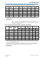
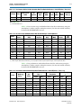
Table 1–6 lists resource usage with buffered burst data flow architecture, using the 4
multipliers/2 adders complex multiplier structure, for data and twiddle width 16, for
Cyclone III (EP3C25F324C6) devices.
Table 1–6. Resource Usage with Buffered Burst Data Flow Architecture—Cyclone III Devices (Part 1 of 2)
Points
256
1024
(2)
(2)
November 2012
Number of
Engines (1)
Combinational
LUTs
Logic
Registers
Memory
(Bits)
Memory
(M9K)
9×9
Blocks
fMAX
(MHz)
1
3129
3778
30,76
16
24
247
1
3234
3976
123136
16
24
241
Altera Corporation
FFT MegaCore Function
User Guide
1–6
Chapter 1: About This MegaCore Function
Performance and Resource Utilization
Table 1–6. Resource Usage with Buffered Burst Data Flow Architecture—Cyclone III Devices (Part 2 of 2)
Points
Number of
Engines (1)
Combinational
LUTs
Logic
Registers
Memory
(Bits)
Memory
(M9K)
9×9
Blocks
fMAX
(MHz)
4096
1
3291
4160
491776
60
24
227
2
5161
5961
30976
31
48
225
2
5270
6169
123136
31
48
207
4096
2
5337
6361
491776
60
48
215
256
4
9015
10738
30976
60
96
230
1024
4
9145
10963
123136
60
96
230
4096
4
9241
11169
491776
60
96
215
256
(3)
(3)
1024
Notes to Table 1–6:
(1) When using the buffered burst architecture, you can specify the number of quad-output FFT engines in the FFT parameter editor.
(2) EP3C10F256C6 device.
(3) EP3C16F484C6 device.
Table 1–7 lists performance with buffered burst data flow architecture, using the 4
multipliers/2 adders complex multiplier structure, for data and twiddle width 16, for
Cyclone III (EP3C25F324C6) devices.
Table 1–7. Performance with the Buffered Burst Data Flow Architecture—Cyclone III Devices
Points
256
Number of
Engines (1)
(4)
fMAX
(MHz)
Transform Calculation
Time (2)
Data Load & Transform
Calculation
Block Throughput
(3)
Cycles
Time (μs)
Cycles
Time (μs)
Cycles
Time (μs)
1
247
235
0.95
491
1.99
331
1.34
1
241
1069
4.44
2093
8.69
1291
5.36
1
227
5167
22.81
9263
40.9
6157
27.18
2
225
162
0.72
397
1.77
299
1.33
2
207
557
2.69
1581
7.63
1163
5.61
4096
2
215
2,07
12.12
6703
31.17
5133
23.87
(4)
1024
4096
256
(5)
1024
(5)
256
4
230
118
0.51
347
1.51
283
1.23
1024
4
230
340
1.48
1364
5.93
1099
4.78
4096
4
215
1378
6.4
5474
25.4
4633
21.5
Notes to Table 1–7:
(1) When using the buffered burst architecture, you can specify the number of quad-output engines in the FFT parameter editor. You may choose
from one, two, or four quad-output engines in parallel.
(2) In a buffered burst data flow architecture, transform time is defined as the time from when the N-sample input block is loaded until the first
output sample is ready for output. Transform time does not include the additional N-1 clock cycle to unload the full output data block.
(3) Block throughput is the minimum number of cycles between two successive start-of-packet (sink_sop) pulses.
(4) EP3C10F256C6 device.
(5) EP3C16F484C6 device.
FFT MegaCore Function
User Guide
November 2012 Altera Corporation
Chapter 1: About This MegaCore Function
Performance and Resource Utilization
1–7
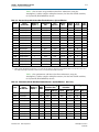
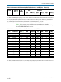
Table 1–8 lists resource usage with burst data flow architecture, using the
4 multipliers/2 adders complex multiplier structure, for data and twiddle width 16,
for Cyclone III (EP3C10F256C6) devices.
Table 1–8. Resource Usage with the Burst Data Flow Architecture—Cyclone III Devices
Engine
Architecture
Points
Number of
Engines (2)
Combinational
LUTs
Logic
Registers
Memory
(Bits)
Memory
(M9K)
9×9
Blocks
fMAX
(MHz)
256
Quad Output
1
3120
3694
14592
8
24
232
1024
Quad Output
1
3227
3876
57600
8
24
246
4096
Quad Output
1
3277
4044
229632
28
24
215
256
Quad Output
2
5141
5872
14592
15
48
244
1024
Quad Output
2
5248
6064
57600
15
48
216
4096
Quad Output
2
5304
6240
229632
28
48
219
256
Quad Output
4
9012
10659
14592
28
96
225
1024
Quad Output
4
9144
10868
57600
28
96
202
4096
Quad Output
4
9241
11058
229632
28
96
204
256
Single Output
1
1449
1499
9472
3
8
250
1024
Single Output
1
1518
1545
37120
6
8
223
4096
Single Output
1
1598
1591
147712
19
8
227
256
Single Output
2
2131
2460
14592
9
16
235
1024
Single Output
2
2185
2536
57600
11
16
221
4096
Single Output
2
2237
2612
229632
28
16
219
Note to Table 1–8:
(1) When using the burst data flow architecture, you can specify the number of engines in the FFT parameter editor. You may choose from one to
two single-output engines in parallel, or from one, two, or four quad-output engines in parallel.
Table 1–9 lists performance with burst data flow architecture, using the
4 multipliers/2 adders complex multiplier structure, for data and twiddle width 16,
for Cyclone III (EP3C10F256C6) devices.
Table 1–9. Performance with the Burst Data Flow Architecture—Cyclone III Devices (Part 1 of 2)
Engine
Architecture
Points
Number of
Engines (1)
fMAX
(MHz)
Transform
Calculation Time
(2)
Data Load & Transform
Calculation
Block Throughput
(3)
Cycles
Time (μs)
Cycles
Time (μs)
Cycles
Time (μs)
256
Quad Output
1
232
235
1.01
491
2.12
331
1.43
1024
Quad Output
1
246
1069
4.35
2093
8.51
1291
5.25
4096
Quad Output
1
215
5167
24.07
9263
43.15
6157
28.68
256
Quad Output
2
244
162
0.66
397
1.63
299
1.23
1024
Quad Output
2
216
557
2.58
1581
7.31
1163
5.38
4096
Quad Output
2
219
2607
11.9
6703
30.59
5133
23.43
256
Quad Output
4
225
118
0.52
374
1.66
283
1.26
1024
Quad Output
4
202
340
1.68
1364
6.75
1099
5.43
4096
Quad Output
4
204
1378
6.76
5474
26.87
4633
22.74
256
Single Output
1
250
1115
4.45
1371
5.48
1628
6.5
November 2012
Altera Corporation
FFT MegaCore Function
User Guide
1–8
Chapter 1: About This MegaCore Function
Performance and Resource Utilization
Table 1–9. Performance with the Burst Data Flow Architecture—Cyclone III Devices (Part 2 of 2)
Engine
Architecture
Points
Number of
Engines (1)
fMAX
(MHz)
Transform
Calculation Time
(2)
Data Load & Transform
Calculation
Block Throughput
(3)
Cycles
Time (μs)
Cycles
Time (μs)
Cycles
Time (μs)
1024
Single Output
1
223
5230
23.43
6344
28.42
7279
32.6
4096
Single Output
1
227
24705
108.7
28801
126.73
32898
144.75
256
Single Output
2
235
585
2.49
841
3.58
1098
4.67
1024
Single Output
2
221
2652
12
3676
16.64
4701
21.28
4096
Single Output
2
219
12329
56.28
16495
75.3
20605
94.06
Notes to Table 1–9:
(1) In the burst I/O data flow architecture, you can specify the number of engines in the FFT parameter editor. You may choose from one to two
single-output engines in parallel, or from one, two, or four quad-output engines in parallel.
(2) Transform time is the time frame when the input block is loaded until the first output sample (corresponding to the input block) is output.
Transform time does not include the time to unload the full output data block.
(3) Block throughput is defined as the minimum number of cycles between two successive start-of-packet (sink_sop) pulses.
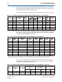
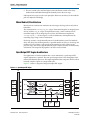
Stratix III Devices
Table 1–10 lists the streaming data flow performance, using the 4 multipliers/2 adders
complex multiplier structure, for data and twiddle width 16, for Stratix III
(EP3SE50F780C2) devices.
Table 1–10. Performance with the Streaming Data Flow Engine Architecture—Stratix III Devices
Points
Combinational
ALUTs
Logic
Registers
Memory
(Bits)
Memory
(M9K)
18 × 18
Blocks
fMAX
(MHz)
Clock
Cycle
Count
Transform
Time (μs)
256
2094
3715
39168
20
12
442
256
0.58
1024
2480
4458
155904
20
12
413
10024
2.48
4096
2357
4545
622848
76
12
388
4096
10.57
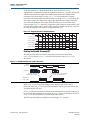
Table 1–11 lists the variable streaming data flow performance, with in order inputs
and bit-reversed outputs, for width 16 (32 for floating point), for Stratix III
(EP3SE50F780C2) devices.
1
The variable streaming with fixed-point number representation uses natural word
growth, therefore the multiplier requirement is larger compared with the equivalent
streaming FFT with the same number of points.
If you want to significantly reduce M9K memory utilization, set a lower fMAX target.
Table 1–11. Performance with the Variable Streaming Data Flow Engine Architecture—Stratix III Devices (Part 1 of 2)
Point Type
Points
Combinational
ALUTs
Logic
Registers
Memory
(Bits)
Memory
(M9K)
18 × 18
Blocks
fMAX
(MHz)
Clock
Cycle
Count
Transform
Time (μs)
Fixed
256
2511
3927
10239
16
20
341
256
0.75
Fixed
1024
3476
5244
42218
23
28
323
1024
3.17
Fixed
4096
4480
6628
170639
42
36
320
4096
12.8
Floating
256
14059
13424
34728
64
48
303
256
0.84
FFT MegaCore Function
User Guide
November 2012 Altera Corporation
Chapter 1: About This MegaCore Function
Performance and Resource Utilization
1–9
Table 1–11. Performance with the Variable Streaming Data Flow Engine Architecture—Stratix III Devices (Part 2 of 2)
Point Type
Points
Combinational
ALUTs
Logic
Registers
Memory
(Bits)
Memory
(M9K)
18 × 18
Blocks
fMAX
(MHz)
Clock
Cycle
Count
Transform
Time (μs)
Floating
1024
18019
16560
140750
95
64
286
1024
3.58
4096
22026
19717
568579
150
80
286
4096
14.33
Floating
(1)
Note to Table 1–11:
(1) EP3SL70F780C2 device.
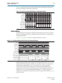
Table 1–12 lists resource usage with buffered burst data flow architecture, using the
4 multipliers/2 adders complex multiplier structure, for data and twiddle width 16,
for Stratix III (EP3SE50F780C2) devices.
Table 1–12. Resource Usage with Buffered Burst Data Flow Architecture—Stratix III Devices
Points
Number of
Engines (1)
Combinational
ALUTs
Logic
Registers
Memory
(Bits)
Memory
(M9K)
18 × 18
Blocks
fMAX
(MHz)
256
1
1952
3586
30976
16
12
408
1024
1
1989
3784
123136
16
12
390
4096
1
2031
3968
491776
60
12
382
256
2
3261
5577
30976
31
24
365
1024
2
3306
5785
123136
31
24
369
4096
2
3348
5977
491776
60
24
390
256
4
5712
9971
30976
60
48
341
1024
4
5775
10195
123136
60
48
349
4096
4
5857
10403
491776
60
48
325
Note to Table 1–12:
(1) When using the buffered burst architecture, you can specify the number of quad-output FFT engines in the FFT parameter editor.
Table 1–13 lists performance with buffered burst data flow architecture, using the
4 multipliers/2 adders complex multiplier structure, for data and twiddle width 16,
for Stratix III (EP3SE50F780C2) devices.
Table 1–13. Performance with the Buffered Burst Data Flow Architecture—Stratix III Devices (Part 1 of 2)
Points
Number of
Engines (1)
fMAX
(MHz))
Transform Calculation
Time (2)
Data Load & Transform
Calculation
Block Throughput
(3)
Cycles
Time (μs)
Cycles
Time (μs)
Cycles
Time (μs)
256
1
408
235
0.58
491
1.2
331
0.81
1024
1
390
1069
2.74
2093
5..37
1291
3.31
4096
1
382
5167
13.54
9263
24.27
6157
16.13
256
2
365
162
0.44
397
1.09
299
0.82
1024
2
369
557
1.51
1581
4.29
1163
3.15
4096
2
390
2607
6.68
6703
17.17
5133
13.15
256
4
341
118
0.35
347
1.02
283
0.83
1024
4
349
340
0.98
1364
3.91
1099
3.15
November 2012
Altera Corporation
FFT MegaCore Function
User Guide
1–10
Chapter 1: About This MegaCore Function
Performance and Resource Utilization
Table 1–13. Performance with the Buffered Burst Data Flow Architecture—Stratix III Devices (Part 2 of 2)
Points
Number of
Engines (1)
4096
4
fMAX
(MHz))
325
Transform Calculation
Time (2)
Data Load & Transform
Calculation
Block Throughput
(3)
Cycles
Time (μs)
Cycles
Time (μs)
Cycles
Time (μs)
1378
4.25
5474
16.87
4633
14.27
Notes to Table 1–13:
(1) When using the buffered burst architecture, you can specify the number of quad-output engines in the FFT parameter editor. You may choose
from one, two, or four quad-output engines in parallel.
(2) In a buffered burst data flow architecture, transform time is defined as the time from when the N-sample input block is loaded until the first
output sample is ready for output. Transform time does not include the additional N-1 clock cycle to unload the full output data block.
(3) Block throughput is the minimum number of cycles between two successive start-of-packet (sink_sop) pulses.
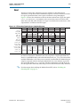
Table 1–14 lists resource usage with burst data flow architecture, using the
4 multipliers/2 adders complex multiplier structure, for data and twiddle width 16,
for Stratix III (EP3SE50F780C2) devices.
Table 1–14. Resource Usage with the Burst Data Flow Architecture—Stratix III Devices
Points
Engine
Architecture
Number of
Engines (2)
Combinational
ALUTs
Logic
Registers
Memory
(Bits)
Memory
(M9K)
18 × 18
Blocks
fMAX
(MHz)
256
Quad Output
1
1796
3502
14592
8
12
408
1024
Quad Output
1
1830
3686
57600
8
12
429
4096
Quad Output
1
1882
3852
229632
28
12
410
256
Quad Output
2
2968
5489
14592
15
24
382
1024
Quad Output
2
3015
5681
57600
15
24
388
4096
Quad Output
2
3054
5856
229632
28
24
386
256
Quad Output
4
5162
9891
14592
28
48
348
1024
Quad Output
4
5213
10100
57600
28
48
380
4096
Quad Output
4
5283
10290
229632
28
48
367
256
Single Output
1
704
1435
9472
3
4
438
1024
Single Output
1
740
1481
37120
6
4
414
4096
Single Output
1
805
1527
147712
19
4
404
256
Single Output
2
1037
2332
14592
9
8
413
1024
Single Output
2
1050
2408
57600
11
8
402
4096
Single Output
2
1092
2484
229632
28
8
406
Notes to Table 1–14:
(1) Represents data and twiddle factor precision.
(2) When using the burst data flow architecture, you can specify the number of engines in the FFT parameter editor. You may choose from one to
two single-output engines in parallel, or from one, two, or four quad-output engines in parallel.
FFT MegaCore Function
User Guide
November 2012 Altera Corporation
Chapter 1: About This MegaCore Function
Performance and Resource Utilization
1–11
Table 1–15 lists performance with burst data flow architecture, using the
4 multipliers/2 adders complex multiplier structure, for data and twiddle width 16,
for Stratix III (EP3SE50F780C2) devices.
Table 1–15. Performance with the Burst Data Flow Architecture—Stratix III Devices
Points
Engine
Architecture
Number of
Engines
(1)
fmax
(MHz)
Transform
Calculation Time
(2)
Data Load &
Transform Calculation
Block Throughput
(3)
Cycles
Time (μs)
Cycles
Time (μs)
Cycles
Time (μs)
1.2
331
0.81
256
Quad Output
1
408
235
0.58
491
1024
Quad Output
1
429
1069
2.49
2093
4.87
1291
3.01
4096
Quad Output
1
410
5167
12.6
9263
22.59
6157
15.02
256
Quad Output
2
382
162
0.42
397
1.04
299
0.78
1024
Quad Output
2
388
557
1.43
1581
4.07
1163
3.00
4096
Quad Output
2
386
2607
6.76
6703
17.39
5133
13.31
256
Quad Output
4
348
118
0.34
374
1.07
283
0.81
1024
Quad Output
4
380
340
0.9
1364
3.59
1099
2.9
4096
Quad Output
4
367
1378
3.76
5474
14.92
4633
12.63
256
Single Output
1
438
1115
2.54
1371
3.13
1628
3.72
1024
Single Output
1
414
5230
12.63
6344
15.31
7279
17.57
4096
Single Output
1
404
24705
61.22
28801
71.37
32898
81.52
256
Single Output
2
413
585
1.42
841
2.04
1098
2.66
1024
Single Output
2
402
2652
6.6
3676
9.15
4701
11.71
4096
Single Output
2
406
12329
30.34
16495
40.59
20605
50.71
Notes to Table 1–15:
(1) In the burst I/O data flow architecture, you can specify the number of engines in the FFT parameter editor. You may choose from one to two
single-output engines in parallel, or from one, two, or four quad-output engines in parallel.
(2) Transform time is the time frame when the input block is loaded until the first output sample (corresponding to the input block) is output.
Transform time does not include the time to unload the full output data block.
(3) Block throughput is defined as the minimum number of cycles between two successive start-of-packet (sink_sop) pulses.
Stratix IV Devices
Table 1–16 lists the streaming data flow performance, using the 4 multipliers/2 adders
complex multiplier structure, for data and twiddle width 16, for Stratix IV
(EP4SGX70DF29C2X) devices.
Table 1–16. Performance with the Streaming Data Flow Engine Architecture—Stratix IV Devices
Points
Combinational
ALUTs
Logic
Registers
Memory
(Bits)
Memory
(M9K)
18 × 18
Blocks
fMAX
(MHz)
Clock
Cycle
Count
Transform
Time (μs)
256
2092
3714
39,68
20
12
436
256
0.59
1024
2480
4458
155904
20
12
437
1024
2.34
4096
2356
4545
622848
76
12
419
4096
9.78
Table 1–17 lists the variable streaming data flow performance, with in order inputs
and bit-reversed outputs, for width 16 (32 for floating point), for Stratix IV
(EP4SGX70DF29C2X) devices.
November 2012
Altera Corporation
FFT MegaCore Function
User Guide
1–12
Chapter 1: About This MegaCore Function
Performance and Resource Utilization
1
The variable streaming with fixed-point number representation uses natural word
growth, therefore the multiplier requirement is larger compared with the equivalent
streaming FFT with the same number of points.
If you want to significantly reduce M9K memory utilization, set a lower fMAX target.
Table 1–17. Performance with the Variable Streaming Data Flow Engine Architecture—Stratix IV Devices
Point Type
Points
Memory
Combinational
ALUTs
Logic
Registers
Bits
M9K
18 × 18
Blocks
fMAX
(MHz)
Clock
Cycle
Count
Transform
Time (μs)
Fixed
256
2517
4096
10239
10
20
323
256
0.79
Fixed
1024
3489
5433
42218
15
28
329
1024
3.12
Fixed
4096
4503
6936
170639
33
36
327
4096
12.52
Floating
256
18024
16714
140750
61
48
320
256
0.8
Floating
1024
14063
13502
34728
89
64
314
1024
3.26
Floating
4096
22030
19806
568579
146
80
310
4096
13.23
Table 1–18 lists resource usage with buffered burst data flow architecture, using the
4 multipliers/2 adders complex multiplier structure, for data and twiddle width 16,
for Stratix IV (EP4SGX70DF29C2X) devices.
Table 1–18. Resource Usage with Buffered Burst Data Flow Architecture—Stratix IV Devices
Points
Number of
Engines (1)
Combinational
ALUTs
Logic
Registers
Memory
(Bits)
Memory
(M9K)
18 × 18
Blocks
fMAX
(MHz)
256
1
1951
3586
30976
16
12
443
1024
1
1990
3784
123136
16
12
441
4096
1
2034
3968
491776
60
12
421
256
2
3262
5577
30976
31
24
428
1024
2
3307
5785
123136
31
24
410
4096
2
3348
5977
491776
60
24
393
256
4
5712
9970
30976
60
48
368
1024
4
5774
10195
123136
60
48
362
4096
4
5856
10401
491776
60
48
368
Notes to Table 1–18:
(1) When using the buffered burst architecture, you can specify the number of quad-output FFT engines in the FFT parameter editor.
Table 1–19 lists performance with buffered burst data flow architecture, using the
4 multipliers/2 adders complex multiplier structure, for data and twiddle width 16,
for Stratix IV (EP4SGX70DF29C2X) devices.
Table 1–19. Performance with the Buffered Burst Data Flow Architecture—Stratix IV Devices (Part 1 of 2)
Points
Number of
Engines (1)
fMAX (MHz)
Transform Calculation
Time (2)
Data Load & Transform
Calculation
Block Throughput
(3)
Cycles
Time (μs)
Cycles
Time (μs)
Cycles
Time (μs)
256
1
443
235
0.53
491
1.11
331
0.75
1024
1
441
1069
2.42
2093
4.75
1291
2.93
FFT MegaCore Function
User Guide
November 2012 Altera Corporation
Chapter 1: About This MegaCore Function
Performance and Resource Utilization
1–13
Table 1–19. Performance with the Buffered Burst Data Flow Architecture—Stratix IV Devices (Part 2 of 2)
Number of
Engines (1)
Points
fMAX (MHz)
Transform Calculation
Time (2)
Data Load & Transform
Calculation
Block Throughput
(3)
Cycles
Time (μs)
Cycles
Time (μs)
Cycles
Time (μs)
4096
1
421
5167
12.26
9263
21.98
6157
14.61
256
2
428
162
0.38
397
0.93
299
0.7
1024
2
410
557
1.36
1581
3.85
1163
2.84
4096
2
393
2607
6.64
6703
17.07
5133
13.07
256
4
368
118
0.32
347
0.94
283
0.77
1024
4
362
340
0.94
1364
3.77
1099
3.04
4096
4
368
1378
3.75
5474
14.89
4633
12.61
Notes to Table 1–19:
(1) When using the buffered burst architecture, you can specify the number of quad-output engines in the FFT parameter editor. You may choose
from one, two, or four quad-output engines in parallel.
(2) In a buffered burst data flow architecture, transform time is defined as the time from when the N-sample input block is loaded until the first
output sample is ready for output. Transform time does not include the additional N-1 clock cycle to unload the full output data block.
(3) Block throughput is the minimum number of cycles between two successive start-of-packet (sink_sop) pulses.
Table 1–20 lists resource usage with burst data flow architecture, using the
4 multipliers/2 adders complex multiplier structure, for data and twiddle width 16,
for Stratix IV (EP4SGX70DF29C2X) devices.
Table 1–20. Resource Usage with the Burst Data Flow Architecture—Stratix IV Devices
Engine
Architecture
Points
Number of
Engines (2)
Combinational
ALUTs
Logic
Registers
Memory
(Bits)
Memory
(M9K)
18 × 18
Blocks
fMAX
(MHz)
256
Quad Output
1
1794
3502
14592
8
12
436
1024
Quad Output
1
1829
3684
57600
8
12
446
4096
Quad Output
1
1881
3852
229632
28
12
443
256
Quad Output
2
2968
5489
14592
15
24
418
1024
Quad Output
2
3014
5680
57600
15
24
412
4096
Quad Output
2
3053
5856
229632
28
24
366
256
Quad Output
4
5160
9891
14592
28
48
369
1024
Quad Output
4
5218
10101
57600
28
48
385
4096
Quad Output
4
5284
10290
229632
28
48
380
256
Single Output
1
704
1436
9472
3
4
407
1024
Single Output
1
740
1482
37120
6
4
413
4096
Single Output
1
801
1528
147712
19
4
412
256
Single Output
2
1036
2332
14592
9
8
405
1024
Single Output
2
1052
2408
57600
11
8
431
4096
Single Output
2
1092
2484
229632
28
8
406
Notes to Table 1–20:
(1) Represents data and twiddle factor precision.
(2) When using the burst data flow architecture, you can specify the number of engines in the FFT parameter editor. You may choose from one to
two single-output engines in parallel, or from one, two, or four quad-output engines in parallel.
November 2012
Altera Corporation
FFT MegaCore Function
User Guide
1–14
Chapter 1: About This MegaCore Function
Performance and Resource Utilization
Table 1–21 lists performance with burst data flow architecture, using the
4 multipliers/2 adders complex multiplier structure, for data and twiddle width 16,
for Stratix IV (EP4SGX70DF29C2X) devices.
Table 1–21. Performance with the Burst Data Flow Architecture—Stratix IV Devices
Points
Engine
Architecture
Number of
Engines (1)
fMAX
(MHz)
Transform
Calculation Time
(2)
Data Load & Transform
Calculation
Block Throughput
(3)
Cycles
Time (μs)
Cycles
Time (μs)
Cycles
Time (μs)
0.54
491
1.12
331
0.76
256
Quad Output
1
436
235
1024
Quad Output
1
446
1069
2.39
2093
4.69
1291
2.89
4096
Quad Output
1
443
5167
11.66
9263
20.9
6157
13.89
256
Quad Output
2
418
162
0.39
397
0.95
299
0.71
1024
Quad Output
2
412
557
1.35
1581
3.83
1163
2.82
4096
Quad Output
2
366
2607
7.12
6703
18.3
5133
14.01
256
Quad Output
4
369
118
0.32
374
1.01
283
0.77
1024
Quad Output
4
385
340
0.88
1364
3.55
1099
2.86
4096
Quad Output
4
380
1378
3.63
5474
14.42
4633
12.20
256
Single Output
1
407
1115
2.74
1371
3.37
1628
4.00
1024
Single Output
1
413
5230
12.66
6344
15.35
7279
17.62
4096
Single Output
1
412
24705
59.91
28801
69.84
32898
79.78
256
Single Output
2
405
585
1.45
841
2.08
1098
2.71
1024
Single Output
2
431
2652
6.16
3676
8.54
4701
10.92
4096
Single Output
2
406
12329
30.35
16495
40.61
20605
50.73
Notes to Table 1–21:
(1) In the burst I/O data flow architecture, you can specify the number of engines in the FFT parameter editor. You may choose from one to two
single-output engines in parallel, or from one, two, or four quad-output engines in parallel.
(2) Transform time is the time frame when the input block is loaded until the first output sample (corresponding to the input block) is output.
Transform time does not include the time to unload the full output data block.
(3) Block throughput is defined as the minimum number of cycles between two successive start-of-packet (sink_sop) pulses.
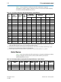
Stratix V Devices
Table 1–22 lists the streaming data flow performance, using the 4 multipliers/2 adders
complex multiplier structure, for data and twiddle width 16, for Stratix V
(5SGXEA7H3F35C2) devices.
Table 1–22. Performance with the Streaming Data Flow Engine Architecture—Stratix V Devices
Points
Combinational
ALUTs
Logic
Registers
Memory
(Bits)
Memory
(M20K)
DSP
Blocks
fMAX
(MHz)
Clock
Cycle
Count
Transform
Time (μs)
256
2,093
3,944
39,168
20
6
395
256
0.65
1024
2,489
4,719
155,904
20
6
382
1,024
2.68
4096
2,352
4,801
622,848
38
6
370
4,096
11.08
FFT MegaCore Function
User Guide
November 2012 Altera Corporation
Chapter 1: About This MegaCore Function
Performance and Resource Utilization
1–15
Table 1–23 lists the variable streaming data flow performance, with in order inputs
and bit-reversed outputs, for width 16 (32 for floating point), for Stratix V
(5SGXEA7H3F35C2) devices.
1
The variable streaming with fixed-point number representation uses natural word
growth, therefore the multiplier requirement is larger compared with the equivalent
streaming FFT with the same number of points.
If you want to significantly reduce M20K memory utilization, set a lower fMAX target.
Table 1–23. Performance with the Variable Streaming Data Flow Engine Architecture—Stratix V Devices
Point Type
Points
M20K
DSP
Blocks
fMAX
(MHz)
Clock
Cycle
Count
Transform
Time (μs)
Memory
Combinational
ALUTs
Logic
Registers
Bits
Fixed
256
2,543
4,319
10,239
15
10
348
256
0.73
Fixed
1024
3,518
5,724
42,204
20
14
330
1,024
3.1
Fixed
4096
4,568
7,290
170,537
31
18
331
4,096
12.36
Floating
256
15,017
15,778
34,445
62
24
334
256
0.77
Floating
1024
19,239
19,551
141,114
91
32
323
1,024
3.17
Floating
4096
23,402
23,295
571,894
121
40
320
4,096
12.82
Table 1–24 lists resource usage with buffered burst data flow architecture, using the
4 multipliers/2 adders complex multiplier structure, for data and twiddle width 16,
for Stratix V (5SGXEA7H3F35C2) devices.
Table 1–24. Resource Usage with Buffered Burst Data Flow Architecture—Stratix IV Devices
Points
Number of
Engines (1)
Combinational
ALUTs
Logic
Registers
Memory
(Bits)
Memory
(M20K)
DSP Blocks
fMAX
(MHz)
256
1
1,958
3,828
30,976
16
6
430
1024
1
1,997
4,042
123,136
16
6
403
4096
1
2,031
4,235
491,776
30
6
402
256
2
3,264
6,053
30,976
30
12
380
1024
2
3,310
6,247
123,136
30
12
379
4096
2
3,344
6,462
491,776
30
12
366
256
4
5,715
10,897
30,976
59
24
337
1024
4
5,776
11,115
123,136
59
24
348
4096
4
5,857
11,341
491,776
59
24
312
Note to Table 1–24:
(1) When using the buffered burst architecture, you can specify the number of quad-output FFT engines in the FFT parameter editor.
November 2012
Altera Corporation
FFT MegaCore Function
User Guide
1–16
Chapter 1: About This MegaCore Function
Performance and Resource Utilization
Table 1–25 lists performance with buffered burst data flow architecture, using the
4 multipliers/2 adders complex multiplier structure, for data and twiddle width 16,
for Stratix V (5SGXEA7H3F35C2) devices.
Table 1–25. Performance with the Buffered Burst Data Flow Architecture—Stratix V Devices
Points
Number of
Engines (1)
fMAX (MHz)
Transform Calculation
Time (2)
Data Load & Transform
Calculation
Block Throughput
(3)
Cycles
Time (μs)
Cycles
Time (μs)
Cycles
Time (μs)
0.55
491
1.14
331
0.77
256
1
430
235
1024
1
403
1,069
2.65
2,093
5.19
1,291
3.2
4096
1
402
5,167
12.86
9,263
23.06
6,157
15.32
256
2
380
162
0.43
397
1.05
299
0.79
1024
2
379
557
1.47
1,581
4.17
1,163
3.07
4096
2
366
2,607
7.13
6,703
18.33
5,133
14.04
256
4
337
118
0.35
347
1.03
283
0.84
1024
4
348
340
0.98
1,364
3.92
1,099
3.16
4096
4
312
1,378
4.42
5,474
17.54
4,633
14.84
Notes to Table 1–25:
(1) When using the buffered burst architecture, you can specify the number of quad-output engines in the FFT parameter editor. You may choose
from one, two, or four quad-output engines in parallel.
(2) In a buffered burst data flow architecture, transform time is defined as the time from when the N-sample input block is loaded until the first
output sample is ready for output. Transform time does not include the additional N-1 clock cycle to unload the full output data block.
(3) Block throughput is the minimum number of cycles between two successive start-of-packet (sink_sop) pulses.
Table 1–26 lists resource usage with burst data flow architecture, using the
4 multipliers/2 adders complex multiplier structure, for data and twiddle width 16,
for Stratix V (5SGXEA7H3F35C2) devices.
Table 1–26. Resource Usage with the Burst Data Flow Architecture—Stratix V Devices
(Part 1 of 2)
Points
Engine
Architecture
Number of
Engines (2)
Combinational
ALUTs
Logic
Registers
Memory
(Bits)
Memory
(M20K)
DSP
Blocks
fMAX
(MHz)
256
Quad Output
1
1,801
3,717
14,592
8
6
414
1024
Quad Output
1
1,833
3,912
57,600
8
6
405
4096
Quad Output
1
1,878
4,078
229,632
14
6
395
256
Quad Output
2
2,970
5,914
14,592
14
12
385
1024
Quad Output
2
3,019
6,129
57,600
14
12
395
4096
Quad Output
2
3,048
6,319
229,632
14
12
374
256
Quad Output
4
5,164
10,743
14,592
27
24
353
1024
Quad Output
4
5,216
10,924
57,600
27
24
314
4096
Quad Output
4
5,280
11,129
229,632
27
24
346
256
Single Output
1
709
1,542
9,472
3
2
445
1024
Single Output
1
751
1,598
37,120
4
2
443
4096
Single Output
1
817
1,637
147,712
9
2
427
256
Single Output
2
1,037
2,521
14,592
8
4
401
1024
Single Output
2
1,052
2,622
57,600
8
4
443
FFT MegaCore Function
User Guide
November 2012 Altera Corporation
Chapter 1: About This MegaCore Function
Performance and Resource Utilization
1–17
Table 1–26. Resource Usage with the Burst Data Flow Architecture—Stratix V Devices
(Part 2 of 2)
Points
Engine
Architecture
Number of
Engines (2)
Combinational
ALUTs
Logic
Registers
Memory
(Bits)
Memory
(M20K)
DSP
Blocks
fMAX
(MHz)
4096
Single Output
2
1,093
2,700
229,632
14
4
366
Notes to Table 1–20:
(1) Represents data and twiddle factor precision.
(2) When using the burst data flow architecture, you can specify the number of engines in the FFT parameter editor. You may choose from one to
two single-output engines in parallel, or from one, two, or four quad-output engines in parallel.
Table 1–27 lists performance with burst data flow architecture, using the
4 multipliers/2 adders complex multiplier structure, for data and twiddle width 16,
for Stratix V (5SGXEA7H3F35C2) devices.
Table 1–27. Performance with the Burst Data Flow Architecture—Stratix V Devices
Points
Engine
Architecture
Number of
Engines (1)
fMAX
(MHz)
Transform
Calculation Time
(2)
Data Load & Transform
Calculation
Block Throughput
(3)
Cycles
Time (μs)
Cycles
Time (μs)
Cycles
Time (μs)
256
Quad Output
1
414
235
0.57
491
1.18
331
0.8
1024
Quad Output
1
405
1,069
2.64
2,093
5.17
1,291
3.19
4096
Quad Output
1
395
5,167
13.08
9,263
23.44
6,157
15.58
256
Quad Output
2
385
162
0.42
397
1.03
299
0.78
1024
Quad Output
2
395
557
1.41
1,581
4
1,163
2.94
4096
Quad Output
2
374
2,607
6.98
6,703
17.94
5,133
13.74
256
Quad Output
4
353
118
0.33
374
1.06
283
0.8
1024
Quad Output
4
314
340
1.08
1,364
4.35
1,099
3.5
4096
Quad Output
4
346
1,378
3.99
5,474
15.84
4,633
13.4
256
Single Output
1
445
1,115
2.51
1,371
3.08
1,628
3.66
1024
Single Output
1
443
5,230
11.79
6,344
14.31
7,279
16.41
4096
Single Output
1
427
24,705
57.86
28,801
67.45
32,898
77.05
256
Single Output
2
401
585
1.46
841
2.1
1,098
2.74
1024
Single Output
2
443
2,652
5.99
3,676
8.3
4,701
10.61
4096
Single Output
2
366
12,239
33.67
16,495
45.05
20,605
56.27
Notes to Table 1–27:
(1) In the burst I/O data flow architecture, you can specify the number of engines in the FFT parameter editor. You may choose from one to two
single-output engines in parallel, or from one, two, or four quad-output engines in parallel.
(2) Transform time is the time frame when the input block is loaded until the first output sample (corresponding to the input block) is output.
Transform time does not include the time to unload the full output data block.
(3) Block throughput is defined as the minimum number of cycles between two successive start-of-packet (sink_sop) pulses.
November 2012
Altera Corporation
FFT MegaCore Function
User Guide
1–18
Chapter 1: About This MegaCore Function
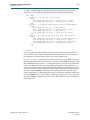
Installation and Licensing
Installation and Licensing
The FFT MegaCore function is part of the MegaCore® IP Library, which is distributed
with the Quartus® II software and can be downloaded from the Altera® website,
www.altera.com.
f For system requirements and installation instructions, refer to the Altera Software
Installation and Licensing manual.
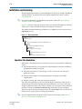
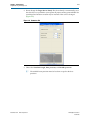
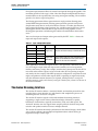
Figure 1–1 shows the directory structure after you install the FFT MegaCore function,
where <path> is the installation directory for the Quartus II software.
The default installation directory on Windows is c:\altera\<version> and on Linux is
/opt/altera<version>.
Figure 1–1. Directory Structure
<path>
Installation directory.
ip
Contains the Altera MegaCore IP Library and third-party IP cores.
altera
Contains the Altera MegaCore IP Library.
common
Contains shared components.
fft
Contains the FFT MegaCore function files.
lib
Contains encrypted lower-level files.
OpenCore Plus Evaluation
With Altera’s free OpenCore Plus evaluation feature, you can perform the following
actions:
■
Simulate the behavior of a megafunction (Altera MegaCore function or AMPPSM
megafunction) within your system.
■
Verify the functionality of your design, as well as evaluate its size and speed
quickly and easily.
■
Generate time-limited device programming files for designs that include
megafunctions.
■
Program a device and verify your design in hardware.
You only need to purchase a license for the FFT MegaCore function when you are
completely satisfied with its functionality and performance, and want to take your
design to production. After you purchase a license, you can request a license file from
the Altera website at www.altera.com/licensing and install it on your computer.
When you request a license file, Altera emails you a license.dat file. If you do not have
Internet access, contact your local Altera representative.
f For more information about OpenCore Plus hardware evaluation, refer to AN 320:
OpenCore Plus Evaluation of Megafunctions.
FFT MegaCore Function
User Guide
November 2012 Altera Corporation
Chapter 1: About This MegaCore Function
Installation and Licensing
1–19
OpenCore Plus Time-Out Behavior
OpenCore Plus hardware evaluation supports the following operation modes:
■
Untethered—the design runs for a limited time.
■
Tethered—requires a connection between your board and the host computer. If
tethered mode is supported by all megafunctions in a design, the device can
operate for a longer time or indefinitely.
All megafunctions in a device time-out simultaneously when the most restrictive
evaluation time is reached. If there is more than one megafunction in a design, a
specific megafunction’s time-out behavior might be masked by the time-out behavior
of the other megafunctions.
The untethered time-out for the FFT MegaCore function is one hour; the tethered
time-out value is indefinite.
The signals source_real, source_imag, and source_exp are forced low when the
evaluation time expires.
November 2012
Altera Corporation
FFT MegaCore Function
User Guide
1–20
FFT MegaCore Function
User Guide
Chapter 1: About This MegaCore Function
Installation and Licensing
November 2012 Altera Corporation
2. Getting Started
Design Flows
The FFT MegaCore function supports the following design flows:
■
DSP Builder: Use this flow if you want to create a DSP Builder model that
includes a FFT MegaCore function variation.
■
MegaWizard™ Plug-In Manager: Use this flow if you would like to create a FFT
MegaCore function variation that you can instantiate manually in your design.
This chapter describes how you can use a FFT MegaCore function in either of these
flows. The parameterization provides the same options in each flow and is described
in “Parameterize the MegaCore Function” on page 2–3.
After parameterizing and simulating a design in either of these flows, you can
compile the completed design in the Quartus II software.
DSP Builder Flow
Altera’s DSP Builder product shortens digital signal processing (DSP) design cycles
by helping you create the hardware representation of a DSP design in an
algorithm-friendly development environment.
DSP Builder integrates the algorithm development, simulation, and verification
capabilities of The MathWorks MATLAB® and Simulink® system-level design tools
with Altera Quartus® II software and third-party synthesis and simulation tools. You
can combine existing Simulink blocks with Altera DSP Builder blocks and MegaCore
function variation blocks to verify system level specifications and perform simulation.
In DSP Builder, a Simulink symbol for the MegaCore function appears in the
MegaCore Functions library of the Altera DSP Builder Blockset in the Simulink library
browser.
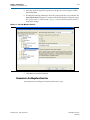
You can use the FFT MegaCore function in the MATLAB/Simulink environment by
performing the following steps:
1. Create a new Simulink model.
2. Select the fft_<version> block from the MegaCore Functions library in the
Simulink Library Browser, add it to your model, and give the block a unique
name.
3. Double-click on the fft_<version> block in your model to display the parameter
editor and parameterize the MegaCore function variation. For an example of
setting parameters for the FFT MegaCore function, refer to “Parameterize the
MegaCore Function” on page 2–3.
4. Click Finish in the parameter editor to complete the parameterization and
generate your FFT MegaCore function variation. For information about the
generated files, refer to Table 2–1 on page 2–11.
5. Connect your FFT MegaCore function variation to the other blocks in your model.
November 2012
Altera Corporation
FFT MegaCore Function
User Guide
2–2
Chapter 2: Getting Started
MegaWizard Plug-In Manager Flow
6. Simulate the MegaCore function variation in your DSP Builder model.
f For more information about the DSP Builder flow, refer to the Using MegaCore
Functions chapter in the DSP Builder User Guide.
1
When you are using the DSP Builder flow, device selection, simulation, Quartus II
compilation and device programming are all controlled within the DSP Builder
environment.
DSP Builder supports integration with SOPC Builder using Avalon® MemoryMapped (Avalon-MM) master/slave and Avalon Streaming (Avalon-ST) source/sink
interfaces.
f For more information about these interface types, refer to the Avalon Interface
Specifications.
MegaWizard Plug-In Manager Flow
The MegaWizard™ Plug-in Manager flow allows you to customize an FFT MegaCore
function, and manually integrate the MegaCore function variation into a Quartus II
design.
Follow the steps below to use the MegaWizard Plug-in Manager flow.
1. Create a new project using the New Project Wizard available from the File menu
in the Quartus II software.
2. Launch MegaWizard Plug-in Manager from the Tools menu, and select the option
to create a new custom megafunction variation (Figure 2–1).
Figure 2–1. MegaWizard Plug-In Manager
3. Click Next and select FFT <version> from the DSP>Transforms section in the
Installed Plug-Ins tab.
4. Verify that the device family is the same as you specified in the New Project
Wizard.
FFT MegaCore Function
User Guide
November 2012 Altera Corporation
Chapter 2: Getting Started
MegaWizard Plug-In Manager Flow
2–3
5. Select the top-level output file type for your design; the wizard supports VHDL
and Verilog HDL.
6. The MegaWizard Plug-In Manager shows the project path that you specified in the
New Project Wizard. Append a variation name for the MegaCore function output
files <project path>\<variation name>. Figure 2–2 shows the wizard after you have
made these settings.
Figure 2–2. Select the MegaCore Function
7. Click Next to launch IP Toolbench.
Parameterize the MegaCore Function
To parameterize your MegaCore function, follow these steps:
November 2012
Altera Corporation
FFT MegaCore Function
User Guide
2–4
Chapter 2: Getting Started
MegaWizard Plug-In Manager Flow
1. Click Step 1: Parameterize in IP Toolbench (Figure 2–3 on page 2–4).
Figure 2–3. IP Toolbench—Parameterize
FFT MegaCore Function
User Guide
November 2012 Altera Corporation
Chapter 2: Getting Started
MegaWizard Plug-In Manager Flow
2–5
2. Do not change the Target Device Family The device family is automatically set to
the value that was specified in your Quartus II project and the generated HDL for
your MegaCore function variation may be incorrect if this value is changed
(Figure 2–4).
Figure 2–4. Parameters Tab
3. Choose the Transform length, Data precision, and Twiddle precision.
1
November 2012
Altera Corporation
The twiddle factor precision must be less than or equal to the data
precision.
FFT MegaCore Function
User Guide
2–6
Chapter 2: Getting Started
MegaWizard Plug-In Manager Flow
4. Click the Architecture tab (Figure 2–5).
Figure 2–5. Architecture Tab
5. Choose the FFT engine architecture, number of parallel FFT engines, and the I/O
data flow.
If you select the Streaming I/O data flow, the FFT MegaCore function
automatically generates a design with a Quad Output FFT engine architecture and
the minimum number of parallel FFT engines for the required throughput.
1
A single FFT engine architecture provides enough performance for up to a
1,024-point streaming I/O data flow FFT.
If you select Variable Streaming I/O data flow, the Transform length (specified
on the Parameters Tab) represents the maximum transform length that can be
performed. All transforms of length 2m where 6 ≤ m ≤ log2(transform length) can be
performed at runtime.
FFT MegaCore Function
User Guide
November 2012 Altera Corporation
Chapter 2: Getting Started
MegaWizard Plug-In Manager Flow
1
2–7
If you select Variable Streaming and Floating Point on the Architecture
tab, the precision (on the Parameters tab) is automatically set to 32, and the
reverse I/O order options (on the Architecture tab) are Digit Reverse
Order.
If you select Variable Streaming I/O data flow, options to set the I/O order and
data representation are visible. The Input Order option allow you to select the
order in which the samples are presented to the FFT. If you select Natural Order,
the FFT expects the order of the input samples to be sequential (1, 2 …, n – 1, n)
where n is the size of the current transform. For Bit Reverse Order, the FFT expects
the input samples to be in bit-reversed order. For Digit Reverse Order, the FFT
expects the input samples to be in digit-reversed order. For –N/2 to N/2, the FFT
expects the input samples to be in the order –N/2 to (N/2) – 1 (also known as DCcentered order). Similarly the Output Order option specifies the order in which
the FFT generates the output. Whether you can select Bit Reverse Order or Digit
Reverse Order depends on your Data Representation selection. You can select
Fixed Point or Floating Point data representation. If you select Fixed Point, the
FFT variation implements the radix-22 architecture and the reverse I/O order
option is Bit Reverse Order; if you select Floating Point, the FFT variation
implements the mixed radix-4/2 architecture and the reverse I/O order option is
Digit Reverse Order.
For sample digit-reversed order, if n is a power of four, the order is radix-4
digit-reversed order, in which two-bit digits in the sample number are units in the
reverse ordering. For example, if n = 16, sample number 4 becomes the second
sample in the sample stream (by reversal of the digits in 0001, the location in the
sample stream, to 0100). However, in mixed radix-4/2 architecture, n need not be a
power of four. If n is not a power of four, the two-bit digits are grouped from the
least significant bit, and the most significant bit becomes the least significant bit in
the digit-reversed order. For example, if n = 512, the sample at location
[8][76][54][32][10] in the digit-reversed sample stream is sample number
[10][32][54][76][8] in the natural ordering. The 261st sample in the stream, at
location 260 (100000100), is the sample that is number 33 (000100001) in the natural
ordering.
November 2012
Altera Corporation
FFT MegaCore Function
User Guide
2–8
Chapter 2: Getting Started
MegaWizard Plug-In Manager Flow
6. Click the Implementation Options tab (Figure 2–6).
Figure 2–6. Implementation Options Tab
7. Choose the complex multiplier implementation.
You can choose a Structure with three multipliers and five adders or four
multipliers and two adders. You can also choose to Implement Multipliers in DSP
blocks only, logic cells only or both DSP blocks and logic cells. If your FFT
variation targets a Stratix V device, you can turn on DSP Resource Optimization.
This option optimizes for area rather than speed by utilizing the new Stratix V
DSP block complex 18 × 25 and 27 × 27 multiplication modes. In the variable
streaming architecture using the floating point representation, the option utilizes
the DSP block complex 27 × 27 multiplication mode at the potential expense of
lower accuracy.
FFT MegaCore Function
User Guide
November 2012 Altera Corporation
Chapter 2: Getting Started
MegaWizard Plug-In Manager Flow
2–9
1
The complex multiplier implementation options Structure and Implement
Multipliers in are not available for the variable streaming architecture. The
complex multiplier implementation option DSP Resource Optimization is
available only in Stratix V devices.
If you turn on DSP Resource Optimization, and your variation has data precision
between 18 and 25 bits, inclusive, and twiddle precision less than or equal to 18
bits, the FFT MegaCore function configures the DSP blocks in complex 18 × 25
multiplication mode. If you turn on DSP Resource Optimization and your
variation does not meet these criteria, the FFT MegaCore function configures the
DSP blocks based on the criteria it uses when you do not turn on the option. The
FFT MegaCore function configures the Stratix V device according to the following
criteria when you turn off the option or it is not available:
■
If data precision and twiddle precision are both less than or equal to 27 bits,
configures 3/4 of a DSP block in complex 27 × 27 multiplication mode. This
configuration uses only three of the four DSP rows in a single DSP block.
■
If data precision is greater than 27 bits and twiddle precision is less than or
equal to 18 bits, configures one DSP block in sum of two 18 × 36 multiplication
mode. This configuration uses four DSP rows.
■
Otherwise, configures two DSP blocks in 36 × 36 multiplication mode. This
configuration uses eight DSP rows in two DSP blocks.
f For more information about the Stratix V DSP block modes, refer to the
Variable Precision DSP Blocks in Stratix V Devices chapter in the Stratix V
Device Handbook.
8. Turn on Global Clock Enable, if you want to add a global clock enable to your
design.
9. Specify the memory options.
You can set memory use balance with the Twiddle ROM Distribution, turn on
Use M-RAM Blocks, and turn on Implement appropriate logic functions in
RAM. If your FFT variation targets an appropriate device family, the Use M144K
Blocks option replaces the Use M-RAM Blocks option.
1
The memory options are not available for the variable streaming
architecture. The memory options Twiddle ROM Distribution and Use
M-RAM Blocks are not available in the Cyclone series of device families
(the Cyclone, Cyclone II, Cyclone III, Cyclone III LS, and Cyclone IV device
families).
10. Click Finish when the implementation options are set.
f For more information about the FFT MegaCore function parameters, refer to Table 3–3
on page 3–14.
November 2012
Altera Corporation
FFT MegaCore Function
User Guide
2–10
Chapter 2: Getting Started
MegaWizard Plug-In Manager Flow
Set Up Simulation
An IP functional simulation model is a cycle-accurate VHDL or Verilog HDL model
produced by the Quartus II software. The model allows for fast functional simulation
of IP using industry-standard VHDL and Verilog HDL simulators.
c You may only use these simulation model output files for simulation purposes and
expressly not for synthesis or any other purposes. Using these models for synthesis
creates a nonfunctional design.
To generate an IP functional simulation model for your MegaCore function, follow
these steps:
1. Click Step 2: Set Up Simulation in IP Toolbench (Figure 2–3 on page 2–4).
2. Turn on Generate Simulation Model (Figure 2–7 on page 2–10).
3. Choose the required language in the Language list.
4. Some third-party synthesis tools can use a netlist that contains only the structure
of the MegaCore function, but not detailed logic, to optimize performance of the
design that contains the MegaCore function. If your synthesis tool supports this
feature, turn on Generate netlist.
5. Click OK.
Figure 2–7. Generate Simulation Model
Generate the MegaCore Function
To generate your MegaCore function, follow these steps:
FFT MegaCore Function
User Guide
November 2012 Altera Corporation
Chapter 2: Getting Started
MegaWizard Plug-In Manager Flow
2–11
1. Click Step 3: Generate in IP Toolbench (Figure 2–3 on page 2–4).
The generation phase may take several minutes to complete. The generation
progress and status is displayed in a report window.
Figure 2–8 shows the generation report.
Figure 2–8. Generation Report
Table 2–1 describes the generated files and other files that may be in your project
directory. The names and types of files specified in the IP Toolbench report vary
based on whether you created your design with VHDL or Verilog HDL
Table 2–1. Generated Files (Part 1 of 2)
Filename
(1)
&
(2)
Description
<variation name>_imag_input.txt
The text file contains input imaginary component random data. This file is read by
the generated VHDL or Verilog HDL MATLAB testbenches.
<variation name>_real_input.txt
Test file containing real component random data. This file is read by the generated
VHDL or Verilog HDL and MATLAB testbenches.
<variation name>.bsf
Quartus II symbol file for the MegaCore function variation. You can use this file in
the Quartus II block diagram editor.
<variation name>.cmp
A VHDL component declaration file for the MegaCore function variation. Add the
contents of this file to any VHDL architecture that instantiates the MegaCore
function.
<variation name>.html
A MegaCore function report file in hypertext markup language format.
<variation name>.qip
A single Quartus II IP file is generated that contains all of the assignments and
other information required to process your MegaCore function variation in the
Quartus II compiler. You are prompted to add this file to the current Quartus II
project when you exit from the MegaWizard.
<variation name>.vo or .vho
VHDL or Verilog HDL IP functional simulation model.
November 2012
Altera Corporation
FFT MegaCore Function
User Guide
2–12
Chapter 2: Getting Started
Simulate the Design
Table 2–1. Generated Files (Part 2 of 2)
(1)
&
(2)
Filename
Description
<variation name>.vhd, or .v
A MegaCore function variation file, which defines a VHDL or Verilog HDL top-level
description of the custom MegaCore function. Instantiate the entity defined by
this file inside of your design. Include this file when compiling your design in the
Quartus II software.
<variation name>_1n1024cos.hex,
<variation name>_2n1024cos.hex,
<variation name>_3n1024cos.hex
Intel hex-format ROM initialization files (not generated for variable streaming
FFT).
<variation name>_1n1024sin.hex,
<variation name>_2n1024sin.hex,
<variation name>_3n1024sin.hex
Intel hex-format ROM initialization files (not generated for variable streaming
FFT).
<variation name>_model.m
MATLAB m-file describing a MATLAB bit-accurate model.
<variation name>_tb.m
MATLAB testbench.
<variation name>_syn.v or
<variation name>_syn.vhd
A timing and resource netlist for use in some third-party synthesis tools.
<variation name>_tb.v or
Verilog HDL or VHDL testbench file.
<variation name>_tb.vhd
<variation name>_nativelink.tcl
Tcl Script that sets up NativeLink in the Quartus II software to natively simulate
the design using selected EDA tools. Refer to “Simulating in Third-Party
Simulation Tools Using NativeLink” on page 2–15.
<variation name>_twr1_opt.hex,
<variation name>_twi1_opt.hex,
<variation name>_twr2_opt.hex,
<variation name>_twi2_opt.hex,
<variation name>_twr3_opt.hex,
<variation name>_twi3_opt.hex,
<variation name>_twr4_opt.hex,
<variation name>_twi4_opt.hex,
Intel hex-format ROM initialization files (variable streaming FFT only).
Notes to Table 2–1:
(1) These files are variation dependent, some may be absent or their names may change.
(2) <variation name> is a prefix variation name supplied automatically by IP Toolbench.
2. After you review the generation report, click Exit to close IP Toolbench. Then click
Yes on the Quartus II IP Files prompt to add the .qip file describing your custom
MegaCore function to the current Quartus II project.
f Refer to the Quartus II Help for more information about the MegaWizard Plug-In
Manager.
You can now integrate your custom MegaCore function variation into your design
and simulate and compile.
Simulate the Design
This section describes the following simulation techniques:
FFT MegaCore Function
User Guide
■
Simulate in the MATLAB Software
■
Simulate with IP Functional Simulation Models
November 2012 Altera Corporation
Chapter 2: Getting Started
Simulate the Design
2–13
■
Simulating in Third-Party Simulation Tools Using NativeLink
Simulate in the MATLAB Software
This section discusses fixed-transform and variable streaming architecture
simulations.
Fixed Transform Architectures
The FFT MegaCore function outputs a bit-accurate MATLAB model <variation
name>_model.m, which you can use to model the behavior of your custom FFT
variation in the MATLAB software. The model takes a complex vector as input and it
outputs the transform-domain complex vector and corresponding block exponent
values. The length and direction of the transform (FFT/IFFT) are also passed as inputs
to the model.
If the input vector length is an integral multiple of N, the transform length, the length
of the output vector(s) is equal to the length of the input vector. However, if the input
vector is not an integral multiple of N, it is zero-padded to extend the length to be so.
f For additional information about exponent values, refer to AN 404: FFT/IFFT Block
Floating Point Scaling.
The wizard also creates the MATLAB testbench file <variation name>_tb.m. This file
creates the stimuli for the MATLAB model by reading the input complex random data
from IP Toolbench-generated.
If you selected Floating point data representation, the input data is generated in
hexadecimal format.
To model your fixed-transform architecture FFT MegaCore function variation in the
MATLAB software, follow these steps:
1. Run the MATLAB software.
2. In the MATLAB command window, change to the working directory for your
project.
3. Perform the simulation:
a. Type help <variation name>_model at the command prompt to view the
input and output vectors that are required to run the MATLAB model as a
standalone M-function. Create your input vector and make a function call to
<variation name>_model. For example:
N=2048;
INVERSE = 0; % 0 => FFT 1=> IFFT
x = (2^12)*rand(1,N) + j*(2^12)*rand(1,N);
[y,e] = <variation name>_model(x,N,INVERSE);
or
b. Run the provided testbench by typing the name of the testbench, <variation
name>_tb at the command prompt.
f For more information about MATLAB and Simulink, refer to the MathWorks web site
at www.mathworks.com.
November 2012
Altera Corporation
FFT MegaCore Function
User Guide
2–14
Chapter 2: Getting Started
Simulate the Design
Variable Streaming Architecture
The FFT MegaCore function outputs a bit-accurate MATLAB model <variation
name>_model.m, which you can use to model the behavior of your custom FFT
variation in the MATLAB software. The model takes a complex vector as input and it
outputs the transform-domain complex vector. The lengths and direction of the
transforms (FFT/IFFT) (specified as one entry per block) are also passed as an input to
the model.
You must ensure that the length of the input vector is at least as large as the sum of the
transform sizes for the model to function correctly.
The wizard also creates the MATLAB testbench file <variation name>_tb.m. This file
creates the stimuli for the MATLAB model by reading the input complex random data
from files generated by IP Toolbench.
To model your variable streaming architecture FFT MegaCore function variation in
the MATLAB software, follow these steps:
1. Run the MATLAB software.
2. In the MATLAB command window, change to the working directory for your
project.
3. Perform the simulation:
a. Type help <variation name>_model at the command prompt to view the input
and output vectors that are required to run the MATLAB model as a
standalone M-function. Create your input vector and make a function call to
<variation name>_model. For example:
nps=[256,2048];
inverse = [0,1]; % 0 => FFT 1=> IFFT
x = (2^12)*rand(1,sum(nps)) + j*(2^12)*rand(1,sum(nps));
[y] = <variation name>_model(x,nps,inverse);
or
b. Run the provided testbench by typing the name of the testbench, <variation
name>_tb at the command prompt.
1
If you select bit-reversed output order, you can reorder the data with the
following MATLAB code:
y = y(bit_reverse(0:(FFTSIZE-1), log2(FFTSIZE)) + 1);
where bit_reverse is:
function y = bit_reverse(x, n_bits)
y = bin2dec(fliplr(dec2bin(x, n_bits)));
1
If you select digit-reversed output order, you can reorder the data with the
following MATLAB code:
y = y(digit_reverse(0:(FFTSIZE-1), log2(FFTSIZE)) + 1);
where digit_reverse is:
FFT MegaCore Function
User Guide
November 2012 Altera Corporation
Chapter 2: Getting Started
Simulate the Design
2–15
function y = digit_reverse(x, n_bits)
if mod(n_bits,2)
z = dec2bin(x, n_bits);
for i=1:2:n_bits-1
p(:,i) = z(:,n_bits-i);
p(:,i+1) = z(:,n_bits-i+1);
end
p(:,n_bits) = z(:,1);
y=bin2dec(p);
else
y=digitrevorder(x,4);
end
Simulate with IP Functional Simulation Models
To simulate your design, use the IP functional simulation models generated by IP
Toolbench. The IP functional simulation model is the .vo or .vho file generated as
specified in “Set Up Simulation” on page 2–10. Compile the .vo or .vho file in your
simulation environment to perform functional simulation of your custom variation of
the MegaCore function.
f For more information about IP functional simulation models, refer to the Simulating
Altera Designs chapter in volume 3 of the Quartus II Handbook.
Simulating in Third-Party Simulation Tools Using NativeLink
You can perform a simulation in a third-party simulation tool from within the
Quartus II software, using NativeLink.
f For more information about NativeLink, refer to the Simulating Altera Designs chapter
in volume 3 of the Quartus II Handbook.
You can use the Tcl script file <variation name>_nativelink.tcl to assign default
NativeLink testbench settings to the Quartus II project.
To set up simulation in the Quartus II software using NativeLink, follow these steps:
1. Create a custom variation but ensure you specify your variation name to match the
Quartus II project name.
2. Check that the absolute path to your third-party simulator executable is set. On the
Tools menu click Options and select EDA Tools Options.
3. On the Processing menu, point to Start and click Start Analysis & Elaboration.
4. On the Tools menu, click Tcl scripts. Select the <variation name>_nativelink.tcl Tcl
script and click Run. Check for a message confirming that the Tcl script was
successfully loaded.
5. On the Assignments menu, click Settings, expand EDA Tool Settings and select
Simulation. Select a simulator under Tool Name and in NativeLink Settings,
select Test Benches.
6. On the Tools menu, point to EDA Simulation Tool and click Run EDA RTL
Simulation.
November 2012
Altera Corporation
FFT MegaCore Function
User Guide
2–16
Chapter 2: Getting Started
Compile the Design
Compile the Design
Use the Quartus II software to synthesize and place and route your design. Refer to
Quartus II Help for instructions on performing compilation.
Fixed Transform Architecture
To compile your fixed-transform architecture design, follow these steps:
1. If you are using the Quartus II software to synthesize your design, skip to step 2. If
you are using a third-party synthesis tool to synthesize your design, follow these
steps:
a. Set a black box attribute for your FFT MegaCore function custom variation
before you synthesize the design. Refer to Quartus II Help for instructions on
setting black-box attributes per synthesis tool.
b. Run the synthesis tool to produce an EDIF Netlist File (.edf) or Verilog Quartus
Mapping (VQM) file (.vqm) for input to the Quartus II software.
c. Add the EDIF or VQM file to your Quartus II project.
1
The .qip file supersedes the files you had to add to the project explicitly in previous
versions of the Quartus II software. The .qip file contains the information about the
MegaCore function that the Quartus II software requires.
2. On the Processing menu, click Start Compilation.
Variable Streaming Architecture
To compile your variable streaming architecture design, follow these steps:
1. If you are using the Quartus II software to synthesize your design, skip to step 2. If
you are using a third-party synthesis tool to synthesize your design, follow these
steps:
a. Set a black-box attribute for your FFT MegaCore function custom variation
before you synthesize the design. Refer to Quartus II Help for instructions on
setting black-box attributes per synthesis tool.
b. Run the synthesis tool to produce an EDIF Netlist File (.edf) or Verilog Quartus
Mapping (VQM) file (.vqm) for input to the Quartus II software.
c. Add the EDIF or VQM file to your Quartus II project.
2. On the Project menu, click Add/Remove Files in Project.
3. You can see a list of files in the project. If no files are listed, browse to the \lib
directory, then select and add all files with the prefix auk_dspip_r22sdf. Browse to
the <project> directory and select all files with prefix auk_dspip.
4. On the Processing menu, click Start Compilation.
Program a Device
After you have compiled your design, program your targeted Altera device, and
verify your design in hardware.
FFT MegaCore Function
User Guide
November 2012 Altera Corporation
Chapter 2: Getting Started
Program a Device
2–17
With Altera's free OpenCore Plus evaluation feature, you can evaluate the FFT
MegaCore function before you purchase a license. OpenCore Plus evaluation allows
you to generate an IP functional simulation model, and produce a time-limited
programming file.
f For more information about IP functional simulation models, refer to the Simulating
Altera Designs chapter in volume 3 of the Quartus II Handbook.
You can simulate the FFT in your design, and perform a time-limited evaluation of
your design in hardware.
f For more information about OpenCore Plus hardware evaluation using the FFT, refer
to “OpenCore Plus Evaluation” on page 1–18 and AN 320: OpenCore Plus Evaluation of
Megafunctions.
November 2012
Altera Corporation
FFT MegaCore Function
User Guide
2–18
FFT MegaCore Function
User Guide
Chapter 2: Getting Started
Program a Device
November 2012 Altera Corporation
3. Functional Description
The discrete Fourier transform (DFT), of length N, calculates the sampled Fourier
transform of a discrete-time sequence at N evenly distributed points ωk = 2πk/N on
the unit circle.
The following equation shows the length-N forward DFT of a sequence x(n):
N–1
X[k ] =

x ( n )e
( – j2πnk ) ⁄ N
n=0
where k = 0, 1, ... N – 1
The following equation shows the length-N inverse DFT:
N–1
x(n ) = (1 ⁄ N)

X [ k ]e
( j2πnk ) ⁄ N
k=0
where n = 0, 1, ... N – 1
The complexity of the DFT direct computation can be significantly reduced by using
fast algorithms that use a nested decomposition of the summation in equations one
and two—in addition to exploiting various symmetries inherent in the complex
multiplications. One such algorithm is the Cooley-Tukey radix-r decimation-infrequency (DIF) FFT, which recursively divides the input sequence into N/r sequences
of length r and requires logrN stages of computation.
Each stage of the decomposition typically shares the same hardware, with the data
being read from memory, passed through the FFT processor and written back to
memory. Each pass through the FFT processor is required to be performed logrN
times. Popular choices of the radix are r = 2, 4, and 16. Increasing the radix of the
decomposition leads to a reduction in the number of passes required through the FFT
processor at the expense of device resources.
1
The MegaCore function does not apply the scaling factor 1/N required for a length-N
inverse DFT. You must apply this factor externally.
Buffered, Burst, & Streaming Architectures
A radix-4 decomposition, which divides the input sequence recursively to form
four-point sequences, has the advantage that it requires only trivial multiplications in
the four-point DFT and is the chosen radix in the Altera FFT MegaCore function. This
results in the highest throughput decomposition, while requiring non-trivial complex
multiplications in the post-butterfly twiddle-factor rotations only. In cases where N is
an odd power of two, the FFT MegaCore automatically implements a radix-2 pass on
the last pass to complete the transform.
November 2012
Altera Corporation
FFT MegaCore Function
User Guide
3–2
Chapter 3: Functional Description
Variable Streaming Architecture
To maintain a high signal-to-noise ratio throughout the transform computation, the
FFT MegaCore function uses a block-floating-point architecture, which is a trade-off
point between fixed-point and full-floating point architectures.
In a fixed-point architecture, the data precision needs to be large enough to
adequately represent all intermediate values throughout the transform computation.
For large FFT transform sizes, an FFT fixed-point implementation that allows for
word growth can make either the data width excessive or can lead to a loss of
precision.
In a floating-point architecture each number is represented as a mantissa with an
individual exponent—while this leads to greatly improved precision, floating-point
operations tend to demand increased device resources.
In a block-floating point architecture, all of the values have an independent mantissa
but share a common exponent in each data block. Data is input to the FFT function as
fixed point complex numbers (even though the exponent is effectively 0, you do not
enter an exponent).
The block-floating point architecture ensures full use of the data width within the FFT
function and throughout the transform. After every pass through a radix-4 FFT, the
data width may grow up to log2 (4√2) = 2.5 bits. The data is scaled according to a
measure of the block dynamic range on the output of the previous pass. The number
of shifts is accumulated and then output as an exponent for the entire block. This
shifting ensures that the minimum of least significant bits (LSBs) are discarded prior
to the rounding of the post-multiplication output. In effect, the block-floating point
representation acts as a digital automatic gain control. To yield uniform scaling across
successive output blocks, you must scale the FFT function output by the final
exponent.
1
In comparing the block-floating point output of the Altera FFT MegaCore function to
the output of a full precision FFT from a tool like MATLAB, you must scale the output
by 2 (–exponent_out) to account for the discarded LSBs during the transform. (Refer to
“Block Floating Point Scaling” on page A–1.)
f For more information about exponent values, refer to AN 404: FFT/IFFT Block Floating
Point Scaling.
Variable Streaming Architecture
The variable streaming architecture uses two different types of architecture,
depending on whether you select the fixed-point data representation or the floating
point representation. If you select the fixed-point data representation, the FFT
variation uses a radix 22 single delay feedback architecture, which is a fully pipelined
architecture. If you select the floating point representation, the FFT variation uses a
mixed radix-4/2 architecture. For a length N transform, log4(N) stages are
concatenated together. The radix 22 algorithm has the same multiplicative complexity
of a fully pipelined radix-4 architecture, but the butterfly unit retains a radix-2
architecture. In the radix-4/2 algorithm, a combination of radix-4 and radix-2
architectures are implemented to achieve the computational advantage of the radix-4
architecture while supporting FFT computation with a wider range of transform
lengths. The butterfly units use the DIF decomposition.
FFT MegaCore Function
User Guide
November 2012 Altera Corporation
Chapter 3: Functional Description
The Avalon Streaming Interface
3–3
Fixed point representation allows for natural word growth through the pipeline. The
maximum growth of each stage is 2 bits. After the complex multiplication the data is
rounded down to the expanded data size using convergent rounding. The overall bit
growth is less than or equal to log2(N)+1.
The floating point internal data representation is single precision floating point
(32-bit, IEEE 754 representation). Floating point operations provide more precise
computation results but are costly in hardware resources. To reduce the amount of
logic required for floating point operations, the variable streaming FFT uses "fused"
floating point kernels. The reduction in logic occurs by fusing together several
floating point operations and reducing the number of normalizations that need to
occur.
You can select input and output orders generated by the FFT. Table 3–1 shows the
input and output order options.
Table 3–1. Input & Output Order Options
Input Order
Output Order
Natural
Bit reversed
Bit reversed
Natural
DC-centered
Bit-reversed
Natural
Natural
Bit reversed
Bit reversed
DC-centered
Natural
Mode
Comments
Engine-only
Requires minimum memory and minimum latency.
Engine with
bit-reversal
At the output, requires an extra N complex memory
words and an additional N clock cycles latency,
where N is the size of the transform.
Some applications for the FFT require an FFT > user operation > IFFT chain. In this
case, choosing the input order and output order carefully can lead to significant
memory and latency savings. For example, consider where the input to the first FFT is
in natural order and the output is in bit-reversed order (FFT is operating in engineonly mode). In this example, if the IFFT operation is configured to accept bit-reversed
inputs and produces natural order outputs (IFFT is operating in engine-only mode),
only the minimum amount of memory is required, which provides a saving of N
complex memory words, and a latency saving of N clock cycles, where N is the size of
the current transform.
The Avalon Streaming Interface
The Avalon-ST interface defines a standard, flexible, and modular protocol for data
transfers from a source interface to a sink interface and simplifies the process of
controlling the flow of data in a datapath.
The Avalon-ST interface signals can describe traditional streaming interfaces
supporting a single stream of data without knowledge of channels or packet
boundaries. Such interfaces typically contain data, ready, and valid signals. The
Avalon-ST interface can also support more complex protocols for burst and packet
transfers with packets interleaved across multiple channels.
The Avalon-ST interface inherently synchronizes multi-channel designs, which allows
you to achieve efficient, time-multiplexed implementations without having to
implement complex control logic.
November 2012
Altera Corporation
FFT MegaCore Function
User Guide
3–4
Chapter 3: Functional Description
FFT Processor Engine Architectures
The Avalon-ST interface supports backpressure, which is a flow control mechanism in
which a sink can signal to a source to stop sending data. The sink typically uses
backpressure to stop the flow of data when its FIFO buffers are full or when there is
congestion on its output. When designing a datapath that includes an FFT MegaCore
function, you may not need backpressure if you know the downstream components
can always receive data. You may achieve a higher clock rate by driving the source
ready signal source_ready of the FFT high, and not connecting the sink ready signal
sink_ready.
The FFT MegaCore function has a READY_LATENCY value of zero.
f For more information about the Avalon-ST interface, refer to the Avalon Interface
Specifications.
FFT Processor Engine Architectures
The FFT MegaCore function can be parameterized to use either quad-output or
single-output engine architecture. To increase the overall throughput of the FFT
MegaCore function, you may also use multiple parallel engines of a variation. This
section discusses the following topics:
■
Radix 22 single-delay feedback architecture for fixed-point variable streaming
variations
■
Mixed radix-4/2 architecture for floating point variable streaming variations
■
Quad-output FFT engine architecture for streaming, buffered burst, and burst
variations
■
Single-output FFT engine architecture for buffered burst and burst variations
Radix-22 Single Delay Feedback Architecture
Radix-22 single delay feedback architecture is a fully pipelined architecture for
calculating the FFT of incoming data. It is similar to radix-2 single delay feedback
architectures. However, the twiddle factors are rearranged such that the
multiplicative complexity is equivalent to a radix-4 single delay feedback architecture.
There are log2(N) stages with each stage containing a single butterfly unit and a
feedback delay unit that delays the incoming data by a specified number of cycles,
halved at every stage. These delays effectively align the correct samples at the input of
the butterfly unit for the butterfly calculations. Every second stage contains a
modified radix-2 butterfly whereby a trivial multiplication by –j is performed before
the radix-2 butterfly operations. The output of the pipeline is in bit-reversed order.
The following scheduled operations occur in the pipeline for an FFT of length N = 16.
1. For the first 8 clock cycles, the samples are fed unmodified through the butterfly
unit to the delay feedback unit.
2. The next 8 clock cycles perform the butterfly calculation using the data from the
delay feedback unit and the incoming data. The higher order calculations are sent
through to the delay feedback unit while the lower order calculations are sent to
the next stage.
FFT MegaCore Function
User Guide
November 2012 Altera Corporation
Chapter 3: Functional Description
FFT Processor Engine Architectures
3–5
3. The next 8 clock cycles feed the higher order calculations stored in the delay
feedback unit unmodified through the butterfly unit to the next stage.
Subsequent data stages use the same principles. However, the delays in the feedback
path are adjusted accordingly.
Mixed Radix-4/2 Architecture
Mixed radix-4/2 architecture combines the advantages of using radix-2 and radix-4
butterflies.
The architecture has ceiling(log4(N)) stages. If transform length is an integral power
of four, all of the log4(N) stages are implemented using a radix-4 architecture. If
transform length is not an integral power of four, the architecture implements
ceiling(log4(N)) – 1 of the stages in a radix-4 architecture, and implements the
remaining stage using a radix-2 architecture.
Each stage contains a single butterfly unit and a feedback delay unit. The feedback
delay unit delays the incoming data by a specified number of cycles; in each stage the
number of cycles of delay is one quarter of the number of cycles of delay in the
previous stage. The delays align the butterfly input samples correctly for the butterfly
calculations. The output of the pipeline is in index-reversed order.
Quad-Output FFT Engine Architecture
For applications in which transform time is to be minimized, a quad-output FFT
engine architecture is optimal. The term quad-output refers to the throughput of the
internal FFT butterfly processor. The engine implementation computes all four radix-4
butterfly complex outputs in a single clock cycle.
Figure 3–1 shows a diagram of the quad-output FFT engine.
Figure 3–1. Quad-Output FFT Engine
SW
SW
RAM
A0
x[k,0]
RAM
A1
x[k,1]
RAM
A2
RAM
A3
-j
-1
G[k,1]
H[k,1]
G[k,2]
H[k,2]
G[k,3]
H[k,3]
-1
j
-1
-j
ROM
0
November 2012
Altera Corporation
H[k,0]
BFPU
RAM
A0
BFPU
RAM
A1
BFPU
RAM
A2
BFPU
RAM
A3
j
-1
x[k,2]
x[k,3]
FFT Engine
G[k,0]
ROM
1
ROM
2
FFT MegaCore Function
User Guide
3–6
Chapter 3: Functional Description
I/O Data Flow Architectures
Complex data samples x[k,m] are read from internal memory in parallel and
re-ordered by switch (SW). Next, the ordered samples are processed by the radix-4
butterfly processor to form the complex outputs G[k,m]. Because of the inherent
mathematics of the radix-4 DIF decomposition, only three complex multipliers are
required to perform the three non-trivial twiddle-factor multiplications on the outputs
of the butterfly processor. To discern the maximum dynamic range of the samples, the
four outputs are evaluated in parallel by the block-floating point units (BFPU). The
appropriate LSBs are discarded and the complex values are rounded and re-ordered
before being written back to internal memory.
Single-Output FFT Engine Architecture
For applications in which the minimum-size FFT function is desired, a single-output
engine is most suitable. The term single-output again refers to the throughput of the
internal FFT butterfly processor. In the engine architecture, a single butterfly output is
computed per clock cycle, requiring a single complex multiplier (Figure 3–2 on
page 3–6).
Figure 3–2. Single-Output FFT Engine Architecture
G[k,0]
x[k,0]
-j
-1
x[k,1]
RAM
FFT Engine
G[k,1]
H[k,m]
j
BFPU
-1
x[k,2]
x[k,3]
RAM
G[k,2]
-1
j
-1
G[k,3]
-j
ROM
I/O Data Flow Architectures
This section describes and illustrates the following I/O data flow architectural
options supported by the FFT MegaCore function:
■
Streaming
■
Variable Streaming
■
Buffered Burst
■
Burst
f For information about setting the architectural parameters in IP Toolbench, refer to
“Parameterize the MegaCore Function” on page 2–3.
FFT MegaCore Function
User Guide
November 2012 Altera Corporation
Chapter 3: Functional Description
I/O Data Flow Architectures
3–7
Streaming
The streaming I/O data flow FFT architecture allows continuous processing of input
data, and outputs a continuous complex data stream without the requirement to halt
the data flow in or out of the FFT function.
Streaming FFT Operation
Figure 3–3 on page 3–7 shows an example simulation waveform.
Following the deassertion of the system reset, the data source asserts sink_valid to
indicate to the FFT function that valid data is available for input. A successful data
transfer occurs when both the sink_valid and the sink_ready are asserted.
When the data transfer is complete, sink_sop is deasserted and the data samples are
loaded in natural order.
For more information about the signals, refer to Table 3–4 on page 3–16.
f For more information about the Avalon-ST interface, refer to the Avalon Interface
Specifications.
Figure 3–3. FFT Streaming Data Flow Architecture Simulation Waveform
clk
reset_n
sink_valid
sink_ready
sink_sop
sink_eop
inverse
sink_real
sink_imag
source_real
source_imag
source_exp
source_ready
source_valid
source_sop
source_eop
EXP0
EXP1
EXP2
EXP3
Figure 3–4 shows the input flow control. When the final sample is loaded, the source
asserts sink_eop and sink_valid for the last data transfer.
Figure 3–4. FFT Streaming Data Flow Architecture Input Flow Control
clk
reset_n
sink_valid
sink_ready
sink_sop
inverse
sink_real
sink_imag
November 2012
Altera Corporation
xr(0)
xi(0)
xr(1) xr(2) xr(3) xr(4) xr(5) xr(6) xr(7)
xi(1) xi(2) xi(3) xi(4) xi(5) xi(6) xi(7)
FFT MegaCore Function
User Guide
3–8
Chapter 3: Functional Description
I/O Data Flow Architectures
To change direction on a block-by-block basis, assert or deassert inverse
(appropriately) simultaneously with the application of the sink_sop pulse (concurrent
with the first input data sample of the block).
When the FFT has completed the transform of the input block, it asserts source_valid
and outputs the complex transform domain data block in natural order. The FFT
function asserts source_sop to indicate the first output sample. Figure 3–5 shows the
output flow control.
Figure 3–5. FFT Streaming Data Flow Architecture Output Flow Control
clk
source_real
source_imag
exponent_out
source_ready
source_valid
source_sop
source_eop
Xr[0]
Xr[1]
Xr[2]
Xr[3]
Xr[4]
Xr[5]
Xr[6]
Xr[7]
Xr[8]
Xr[9]
Xr[10] Xr[11]
Xr[12]
Xi[0]
Xi[1]
Xi[2]
Xi[3]
Xi[4]
Xi[5]
Xi[6]
Xi[7]
Xi[8]
Xi[9]
Xi[10] Xi[11]
Xi[12]
EXP0
After N data transfers, source_eop is asserted to indicate the end of the output data
block (Figure 3–3 on page 3–7).
Enabling the Streaming FFT
The sink_valid signal must be asserted for source_valid to be asserted (and a valid
data output). To extract the final frames of data from the FFT, you need to provide
several frames where the sink_valid signal is asserted and apply the sink_sop and
sink_eop signals in accordance with the Avalon-ST specification.
Variable Streaming
The variable streaming architecture allows continuous streaming of input data and
produces a continuous stream of output data similar to the streaming architecture.
Change the Block Size
You change the size of the FFT on a block-by-block basis by changing the value of the
fftpts simultaneously with the application of the sink_sop pulse (concurrent with
the first input data sample of the block). fftpts uses a binary representation of the
size of the transform, therefore for a block with maximum transfer size of 1,024.
Table 3–2 shows the value of the fftpts signal and the equivalent transform size.
Table 3–2. fftpts and Transform Size
FFT MegaCore Function
User Guide
fftpts
Transform Size
10000000000
1,024
01000000000
512
00100000000
256
00010000000
128
00001000000
64
November 2012 Altera Corporation
Chapter 3: Functional Description
I/O Data Flow Architectures
3–9
To change direction on a block-by-block basis, assert or deassert inverse
(appropriately) simultaneously with the application of the sink_sop pulse (concurrent
with the first input data sample of the block). When the FFT has completed the
transform of the input block, it asserts source_valid and outputs the complex
transform domain data block. The FFT function asserts the source_sop to indicate the
first output sample. The order of the output data depends on the output order that
you select in IP Toolbench. The output of the FFT may be in natural order or bitreversed order. Figure 3–6 shows the output flow control when the output order is bitreversed. If the output order is natural order, data flow control remains the same, but
the order of samples at the output is in sequential order 1..N.
Figure 3–6. Output Flow Control—Bit Reversed Order
clock
source_sop
source_eop
source_valid
source_ready
source_real
x0
x512
x256
x768
x128
x640
x384
x896
x1023
source_imag
x0
x512
x256
x768
x128
x640
x384
x896
x1023
Enabling the Variable Streaming FFT
The FFT processes data when there is valid data transferred to the module
(sink_valid asserted). Figure 3–7 shows the FFT behavior when sink_valid is
deasserted.
Figure 3–7. FFT Behavior When sink_valid is Deasserted
Clock
sink_valid
Frame 1
Frame 2
Input Data
The input data stops,
but the output continues
When the FFT is stopped within
a frame, the output pauses
Output Data
source_valid
When sink_valid is deasserted during a frame, the FFT stalls and no data is
processed until sink_valid is reasserted. This implies that any previous frames that
are still in the FFT also stall.
If sink_valid is deasserted between frames, the data currently in the FFT continues to
be processed and transferred to the output. Figure 3–7 shows the FFT behavior when
sink_valid is deasserted between frames and within a frame.
The FFT may optionally be disabled by deasserting the clk_en signal.
November 2012
Altera Corporation
FFT MegaCore Function
User Guide
3–10
Chapter 3: Functional Description
I/O Data Flow Architectures
Dynamically Changing the FFT Size
When the size of the incoming FFT changes, the FFT stalls the incoming data
(deasserts the sink_ready signal) until all of the previous FFT frames of the previous
FFT size have been processed and transferred to the output. Figure 3–8 shows
dynamically changing the FFT size for engine-only mode.
Figure 3–8. Dynamically Changing the FFT Size
clock
reset_n
sink_valid
sink_ready
sink_sop
sink_eop
fftps
inverse
sink_real
sink_imag
source_real
source_imag
source_ready
source_valid
source_sop
source_eop
The Effect of I/O Order
The order of samples entering and leaving the FFT is determined by your selection in
the Architecture tab under I/O Order. This selection also determines if the FFT is
operating in engine-only mode or engine with bit-reversal or digit-reversal mode.
If the FFT operates in engine-only mode, the output data is available after
approximately N + latency clocks cycles after the first sample was input to the FFT.
Latency represents a small latency through the FFT core and depends on the
transform size. For engine with bit-reversal mode, the output is available after
approximately 2N + latency cycles.
Figure 3–9 shows the data flow output when the FFT is operating in engine-only
mode.
Figure 3–9. Data Flow—Engine-Only Mode
clk
reset_n
sink_valid
sink_ready
sink_sop
sink_eop
sink_real
sink_imag
source_real
source_imag
source_valid
source_sop
source_eop
FFT MegaCore Function
User Guide
November 2012 Altera Corporation
Chapter 3: Functional Description
I/O Data Flow Architectures
3–11
Figure 3–10 shows the data flow output when the FFT is operating in engine with
bit-reversal or digit-reversal mode, respectively
Figure 3–10. Data Flow—Engine with Bit-Reversal or Digit-Reversal Mode
clk
reset_n
sink_valid
sink_ready
sink_sop
sink_eop
sink_real
sink_imag
source_real
source_imag
source_valid
source_sop
source_eop
Buffered Burst
The buffered burst I/O data flow architecture FFT requires fewer memory resources
than the streaming I/O data flow architecture, but the tradeoff is an average block
throughput reduction.
Figure 3–11 on page 3–11 shows an example simulation waveform.
Figure 3–11. FFT Buffered Burst Data Flow Architecture Simulation Waveform
clk
reset_n
sink_vaild
sink_ready
sink_sop
sink_eop
inverse
sink_real
sink_imag
source_real
source_imag
source_exp
source_ready
source_valid
source_sop
source_eop
-13609
-47729
271
31221
-21224
-13609
-47729
271
31221
-21224
EXP0
EXP1
EXP2
EXP3
Following the deassertion of the system reset, the data source asserts sink_valid to
indicate to the FFT function that valid data is available for input. A successful data
transfer occurs when both the sink_valid and the sink_ready are asserted.
The data source loads the first complex data sample into the FFT function and
simultaneously asserts sink_sop to indicate the start of the input block. On the next
clock cycle, sink_sop is deasserted and the following N – 1 complex input data
samples must be loaded in natural order. On the last complex data sample, sink_eop
must be asserted.
November 2012
Altera Corporation
FFT MegaCore Function
User Guide
3–12
Chapter 3: Functional Description
I/O Data Flow Architectures
When the input block is loaded, the FFT function begins computing the transform on
the stored input block. The sink_ready signal is held high as you can transfer the first
few samples of the subsequent frame into the small FIFO at the input. If this FIFO is
filled, the core deasserts the sink_ready signal. It is not mandatory to transfer samples
during sink_ready cycles. Figure 3–12 shows the input flow control.
Figure 3–12. FFT Buffered Burst Data Flow Architecture Input Flow Control
clk
reset_n
sink_valid
sink_ready
sink_sop
inverse
sink_real
sink_imag
xr(0)
xr(1)
xr(2)
xr(3)
xr(4)
xr(5)
xr(6)
xr(7)
xr(8)
xr(9)
xi(0)
xi(1)
xi(2)
xi(3)
xi(4)
xi(5)
xi(6)
xi(7)
xi(8)
xi(9)
Following the interval of time where the FFT processor reads the input samples from
an internal input buffer, it re-asserts sink_ready indicating it is ready to read in the
next input block. The beginning of the subsequent input block must be demarcated by
the application of a pulse on sink_sop aligned in time with the first input sample of
the next block.
As in all data flow architectures, the logical level of inverse for a particular block is
registered by the FFT function at the time of the assertion of the start-of-packet signal,
sink_sop.
When the FFT has completed the transform of the input block, it asserts the
source_valid and outputs the complex transform domain data block in natural order
(Figure 3–13).
Figure 3–13. FFT Buffered Burst Data Flow Architecture Output Flow Control
clk
source_realt
source_imag
source_exp
source_ready
master_source_valid
source_sop
source_eop
Xr[0]
Xr[1]
Xr[2]
Xr[3]
Xr[4]
Xr[5]
Xr[6]
Xr[7]
Xr[8]
Xr[9]
Xr[10]
Xi[0]
Xi[1]
Xi[2]
Xi[3]
Xi[4]
Xi[5]
Xi[6]
Xi[7]
Xi[8]
Xi[9]
Xi[10]
EXP0
Signals source_sop and source_eop indicate the start-of-packet and end-of-packet for
the output block data respectively (Figure 3–11).
1
The sink_valid signal must be asserted for source_valid to be asserted (and a valid
data output). You must therefore leave sink_valid signal asserted at the end of data
transfers to extract the final frames of data from the FFT.
f For information about enabling the buffered burst FFT, refer to “Enabling the
Streaming FFT” on page 3–8.
FFT MegaCore Function
User Guide
November 2012 Altera Corporation
Chapter 3: Functional Description
I/O Data Flow Architectures
3–13
Burst
The burst I/O data flow architecture operates similarly to the buffered burst
architecture, except that the burst architecture requires even lower memory resources
for a given parameterization at the expense of reduced average throughput.
Figure 3–14 shows the simulation results for the burst architecture. Again, the signals
source_valid and sink_ready indicate, to the system data sources and slave sinks
either side of the FFT, when the FFT can accept a new block of data and when a valid
output block is available on the FFT output.
Figure 3–14. FFT Burst Data Flow Architecture Simulation Waveform
clk
reset_n
sink_valid
sink_ready
sink_sop
sink_eop
inverse
sink_real
sink_imag
source_real
source_imag
source_exp
source_ready
source_valid
source_sop
source_eop
EXP0
EXP1
-47729
271
-47729
271
EXP2
In a burst I/O data flow architecture, the core can process a single input block only.
There is a small FIFO buffer at the sink of the block and sink_ready is not deasserted
until this FIFO buffer is full. Thus you can provide a small number of additional input
samples associated with the subsequent input block. It is not mandatory to provide
data to the FFT during sink_ready cycles. The burst architecture can load the rest of
the subsequent FFT frame only when the previous transform has been fully unloaded.
f For information about enabling the buffered burst FFT, refer to “Enabling the
Streaming FFT” on page 3–8.
November 2012
Altera Corporation
FFT MegaCore Function
User Guide
3–14
Chapter 3: Functional Description
Parameters
Parameters
Table 3–3 lists the FFT MegaCore function’s parameters.
Table 3–3. Parameters (Part 1 of 3)
Parameter
Value
Description
Displays the target device family. The device family is normally
preselected by the project specified in the Quartus II software.
Target Device Family
<device family>
The generated HDL for your MegaCore function variation may
be incorrect if this value does not match the value specified in
the Quartus II project.
The device family must be the same as your Quartus II project
device family.
Transform Length
64, 128, 256, 512,
1024, 2048, 4096,
8192, 16384, 32768, or
65536. Variable
streaming also allows 8,
16, 32, 131072, and
262144.
The transform length. For variable streaming, this value is the
maximum FFT length.
Data Precision
8, 10, 12, 14, 16, 18,
20, 24, 28, 32
The data precision. The values 28 and 32 are available for
variable streaming only.
Twiddle Precision
8, 10, 12, 14, 16, 18,
20, 24, 28, 32
The twiddle precision. The values 28 and 32 are available for
variable streaming only. Twiddle factor precision must be less
than or equal to data precision.
FFT Engine Architecture
Quad Output,
Single Output
Number of Parallel FFT Engines 1, 2, 4
For both the Buffered Burst and Burst I/O data flow
architectures, you can choose between one, two, and four
quad-output FFT engines working in parallel. Alternatively, if
you have selected a single-output FFT engine architecture, you
may choose to implement one or two engines in parallel.
Multiple parallel engines reduce the FFT MegaCore function’s
transform time at the expense of device resources—which
allows you to select the desired area and throughput trade-off
point.
For more information about device resource and transform
time trade-offs, refer to ““Parameters” on page 3–14. Not
available for variable streaming or streaming architecture.
I/O Data Flow
Streaming
Variable Streaming
Buffered Burst
Burst
Choose the FFT architecture.
I/O Order
Bit Reverse Order, Digit
Reverse Order, Natural
Order, –N/2 to N/2
The input and output order for data entering and leaving the
FFT (variable streaming architecture only). The Digit Reverse
Order option replaces the Bit Reverse Order in variable
streaming floating point variations.
Data Representation
Fixed Point or Floating
Point
The internal data representation type (variable streaming
architecture only), either fixed point with natural bit-growth or
single precision floating point.
FFT MegaCore Function
User Guide
November 2012 Altera Corporation
Chapter 3: Functional Description
Parameters
3–15
Table 3–3. Parameters (Part 2 of 3)
Parameter
Value
Description
3 Mults/5 Adders
4 Mults/2 Adders
You can implement the complex multiplier structure with four
real multipliers and two adders/subtracters, or three
multipliers, five adders, and some additional delay elements.
The 4 Mults/2 Adders structure uses the DSP block structures
to minimize logic usage, and maximize the DSP block usage.
This option may also improve the push button fMAX. The
5 Mults/3 Adders structure requires fewer DSP blocks, but
more LEs to implement. It may also produce a design with a
lower fMAX. Not available for variable streaming architecture or
in Arria V, Cyclone V, and Stratix V devices.
DSP Blocks/Logic Cells
Logic Cells Only
DSP Blocks Only
Each real multiplication can be implemented in DSP blocks or
LEs only, or using a combination of both. If you use a
combination of DSP blocks and LEs, the FFT MegaCore
function automatically extends the DSP block 18 × 18
multiplier resources with LEs as needed. Not available for
variable streaming architecture or in Arria V, Cyclone V, and
Stratix V devices.
DSP Resource Optimization
On or Off
This option is available in Stratix V devices for all architectures
and representations. You can turn on this option to implement
the complex multiplier structure using Stratix V DSP block
complex 18 × 25 multiplication mode or complex 27 × 27
multiplication mode for better DSP resource utilization, at the
possible expense of speed. In the variable streaming
architecture using the floating point representation, this option
implements the complex multiplier structure using Stratix V
DSP block complex 27 × 27 multiplication mode at the possible
expense of accuracy.
Global clock enable
On or Off
Turn on if you want to add a global clock enable to your design.
100% M4K to 100%
M512 or 100% M9K to
100% MLAB
High-throughput FFT parameterizations can require multiple
shallow ROMs for twiddle factor storage. If your target device
family supports M512 RAM blocks (or MLAB blocks in
Stratix III, Stratix IV, and Stratix V devices), you can choose to
distribute the ROM storage requirement between M4K (M9K in
Stratix III and Stratix IV devices) RAM and M512 (MLAB) RAM
blocks by adjusting the slider bar. Set the slider bar to the far
left to implement the ROM storage completely in M4K (M9K)
RAM blocks; set the slider bar to the far right to implement the
ROM completely in M512 (MLAB) RAM blocks. In Stratix V
devices, replace M4K (M9K) with M20K memory blocks.
Structure
Implement Multipliers in
Twiddle ROM Distribution
Implementing twiddle ROM in M512 (MLAB) RAM blocks can
lead to a more efficient device internal memory bit usage.
Alternatively, this option can be used to conserve M4K (M9K)
RAM blocks used for the storage of FFT data or other storage
requirements in your system.
Not available for variable streaming architecture or in the
Cyclone series of device families.
November 2012
Altera Corporation
FFT MegaCore Function
User Guide
3–16
Chapter 3: Functional Description
Signals
Table 3–3. Parameters (Part 3 of 3)
Parameter
Value
Use M-RAM or M144K blocks
Description
Implements suitable data RAM blocks within the FFT MegaCore
function in M-RAM (M144K in Stratix III and Stratix IV devices)
to reduce M4K (M9K) RAM block usage, in device families that
support M-RAM blocks.
On or Off
Not available for variable streaming architecture, or in the
Cyclone series of device families, or in Stratix V devices.
Implement appropriate logic
functions in RAM
Uses embedded RAM blocks to implement internal logic
functions, for example, tapped delay lines in the FFT MegaCore
function. This option reduces the overall logic element count.
On or Off
Not available for variable streaming architecture.
Signals
Table 3–4 lists the Avalon-ST interface signals.
f For more information about the Avalon-ST interface, refer to the Avalon Streaming
Interface Specification.
Table 3–4. Avalon-ST Signals (Part 1 of 2)
Signal Name
clk
Direction
Input
Avalon-ST Type
clk
Size
1
reset_n
Input
reset_n
1
sink_eop
Input
endofpacket
1
Description
Clock signal that clocks all internal FFT engine
components.
Active-low asynchronous reset signal.This signal
can be asserted asynchronously, but must remain
asserted at least one clk clock cycle and must be
deasserted synchronously with clk.
Refer to the Recommended Design Practices
chapter in volume 1 of the Quartus II Handbook for
a sample circuit that ensures synchronous
deassertion of an active-low reset signal.
Indicates the end of the incoming FFT frame.
Indicates an error has occurred in an upstream
module, because of an illegal usage of the
Avalon-ST protocol. The following errors are
defined (refer to Table 3–6):
sink_error
Input
error
2
■
00 = no error
■
01 = missing start of packet (SOP)
■
10 = missing end of packet (EOP)
■
11 = unexpected EOP
If this signal is not used in upstream modules, set
to zero.
sink_imag
FFT MegaCore Function
User Guide
Input
data
data precision
width
Imaginary input data, which represents a signed
number of data precision bits.
November 2012 Altera Corporation
Chapter 3: Functional Description
Signals
3–17
Table 3–4. Avalon-ST Signals (Part 2 of 2)
Signal Name
Direction
Avalon-ST Type
Size
Description
sink_ready
Output
ready
1
Asserted by the FFT engine when it can accept
data. It is not mandatory to provide data to the FFT
during ready cycles.
sink_real
Input
data
data precision
width
Real input data, which represents a signed number
of data precision bits.
sink_sop
Input
startofpacket
1
Indicates the start of the incoming FFT frame.
sink_valid
Input
valid
1
Asserted when data on the data bus is valid. When
sink_valid and sink_ready are asserted, a data
transfer takes place. Refer to “Enabling the
Variable Streaming FFT” on page 3–9.
source_eop
Output
endofpacket
1
Marks the end of the outgoing FFT frame. Only
valid when source_valid is asserted.
source_error
Output
error
2
Indicates an error has occurred either in an
upstream module or within the FFT module
(logical OR of sink_error with errors generated
in the FFT). Refer to Table 3–6 for error codes.
source_exp
Output
data
6
Streaming, burst, and buffered burst architectures
only. Signed block exponent: Accounts for scaling
of internal signal values during FFT computation.
Output
source_imag
data
(data precision
width + growth)
(1)
source_ready
Input
Output
source_real
ready
data
1
(data precision
width + growth)
(1)
Imaginary output data. For burst, buffered burst,
streaming, and variable streaming floating point
FFTs, the output data width is equal to the input
data width. For variable streaming fixed point FFTs,
the size of the output data is dependent on the
number of stages defined for the FFT and is 2 bits
per radix 22 stage.
Asserted by the downstream module if it is able to
accept data.
Real output data. For burst, buffered burst,
streaming, and variable streaming floating point
FFTs, the output data width is equal to the input
data width. For variable streaming fixed point FFTs,
the size of the output data is dependent on the
number of stages defined for the FFT and is 2 bits
per radix 22 stage.
source_sop
Output
startofpacket
1
Marks the start of the outgoing FFT frame. Only
valid when source_valid is asserted.
source_valid
Output
valid
1
Asserted by the FFT when there is valid data to
output.
Note to Table 3–4:
(1) Variable streaming fixed point FFT only. Growth is log2(N) + 1.
November 2012
Altera Corporation
FFT MegaCore Function
User Guide
3–18
Chapter 3: Functional Description
Signals
Table 3–5 shows the component specific signals.
Table 3–5. Component Specific Signals
Signal Name
Direction
Size
Description
fftpts_in
Input
The number of points in this FFT frame. If this value is not specified, the
log2(maximum
FFT can not be a variable length. The default behavior is for the FFT to
number of points)
have fixed length of maximum points. Only sampled at SOP.
fftpts_out
Output
log2(maximum
The number of points in this FFT frame synchronized to the Avalon-ST
number of points) source interface. Variable streaming only.
inverse
Input
1
Inverse FFT calculated if asserted. Only sampled at SOP.
clk_ena
Input
1
Active-high global clock enable input. If deasserted, the FFT is disabled.
Incorrect usage of the Avalon-ST interface protocol on the sink interface results in a
error on source_error. Table 3–6 defines the behavior of the FFT when an incorrect
Avalon-ST transfer is detected. If an error occurs, the behavior of the FFT is undefined
and you must reset the FFT with reset_n.
Table 3–6. Error Handling Behavior
Error
source_error
Description
Missing SOP
01
Asserted when valid goes high, but there is no start of frame.
Missing EOP
10
Asserted if the FFT accepts N valid samples of an FFT frame, but there is no EOP signal.
Unexpected EOP
11
Asserted if EOP is asserted before N valid samples are accepted.
FFT MegaCore Function
User Guide
November 2012 Altera Corporation
A. Block Floating Point Scaling
The FFT MegaCore function uses block-floating-point (BFP) arithmetic internally to
perform calculations. BFP architecture is a trade-off between fixed-point and full
floating-point architecture.
Unlike an FFT block that uses floating point arithmetic, a block-floating-point FFT
block does not provide an input for exponents. Internally, a complex value integer
pair is represented with a single scale factor that is typically shared among other
complex value integer pairs. After each stage of the FFT, the largest output value is
detected and the intermediate result is scaled to improve the precision. The exponent
records the number of left or right shifts used to perform the scaling. As a result, the
output magnitude relative to the input level is:
output*2-exponent
For example, if exponent = –3, the input samples are shifted right by three bits, and
hence the magnitude of the output is output*23.
Block Floating Point
After every pass through a radix-2 or radix-4 engine in the FFT core, the addition and
multiplication operations cause the data bits width to grow. In other words, the total
data bits width from the FFT operation grows proportionally to the number of passes.
The number of passes of the FFT/IFFT computation depends on the logarithm of the
number of points. Table A–1 on page A–2 shows the possible exponents for
corresponding bit growth.
A fixed-point architecture FFT needs a huge multiplier and memory block to
accommodate the large bit width growth to represent the high dynamic range.
Though floating-point is powerful in arithmetic operations, its power comes at the
cost of higher design complexity such as a floating-point multiplier and a floatingpoint adder. BFP arithmetic combines the advantages of floating-point and fixedpoint arithmetic. BFP arithmetic offers a better signal-to-noise ratio (SNR) and
dynamic range than does floating-point and fixed-point arithmetic with the same
number of bits in the hardware implementation.
In a block-floating-point architecture FFT, the radix-2 or radix-4 computation of each
pass shares the same hardware, with the data being read from memory, passed
through the core engine, and written back to memory. Before entering the next pass,
each data sample is shifted right (an operation called "scaling") if there is a carry-out
bit from the addition and multiplication operations. The number of bits shifted is
based on the difference in bit growth between the data sample and the maximum data
sample detected in the previous stage. The maximum bit growth is recorded in the
exponent register. Each data sample now shares the same exponent value and data bit
width to go to the next core engine. The same core engine can be reused without
incurring the expense of a larger engine to accommodate the bit growth.
The output SNR depends on how many bits of right shift occur and at what stages of
the radix core computation they occur. In other words, the signal-to-noise ratio is data
dependent and you need to know the input signal to compute the SNR.
November 2012
Altera Corporation
FFT MegaCore Function
User Guide
A–2
Appendix A: Block Floating Point Scaling
Calculating Possible Exponent Values
Calculating Possible Exponent Values
Depending on the length of the FFT/IFFT, the number of passes through the radix
engine is known and therefore the range of the exponent is known. The possible
values of the exponent are determined by the following equations:
P = ceil{log4N}, where N is the transform length
R = 0 if log2N is even, otherwise R = 1
Single output range = (–3P+R, P+R–4)
Quad output range = (–3P+R+1, P+R–7)
These equations translate to the values in Table A–1.
Table A–1. Exponent Scaling Values for FFT / IFFT
(1)
Single Output Engine
N
Quad Output Engine
P
Max
(2)
Min
(2)
Max
(2)
Min
64
3
–9
–1
–8
–4
128
4
–11
1
–10
–2
256
4
–12
0
–11
–3
512
5
–14
2
–13
–1
1,024
5
–15
1
–14
–2
2,048
6
–17
3
–16
0
4,096
6
–18
2
–17
–1
8,192
7
–20
4
–19
1
16,384
7
–21
3
–20
0
(2)
Note to Table A–1:
(1) This table lists the range of exponents, which is the number of scale events that occurred internally. For IFFT, the
output must be divided by N externally. If more arithmetic operations are performed after this step, the division by
N must be performed at the end to prevent loss of precision.
(2) The maximum and minimum values show the number of times the data is shifted. A negative value indicates shifts
to the left, while a positive value indicates shifts to the right.
Implementing Scaling
To implement the scaling algorithm, follow these steps:
1. Determine the length of the resulting full scale dynamic range storage register. To
get the length, add the width of the data to the number of times the data is shifted
(the max value in Table A–1). For example, for a 16-bit data, 256-point Quad
Output FFT/IFFT with Max = –11 and Min = –3. The Max value indicates 11 shifts
to the left, so the resulting full scaled data width is 16 + 11, or 27 bits.
2. Map the output data to the appropriate location within the expanded dynamic
range register based upon the exponent value. To continue the above example, the
16-bit output data [15..0] from the FFT/IFFT is mapped to [26..11] for an exponent
of –11, to [25..10] for an exponent of –10, to [24..9] for an exponent of –9, and so on.
3. Sign extend the data within the full scale register.
FFT MegaCore Function
User Guide
November 2012 Altera Corporation
Appendix A: Block Floating Point Scaling
Implementing Scaling
A–3
A sample of Verilog HDL code that illustrates the scaling of the output data (for
exponents –11 to –9) with sign extension is shown in the following example:
case (exp)
6'b110101 : //-11 Set data equal to MSBs
begin
full_range_real_out[26:0] <= {real_in[15:0],11'b0};
full_range_imag_out[26:0] <= {imag_in[15:0],11'b0};
end
6'b110110 : //-10 Equals left shift by 10 with sign extension
begin
full_range_real_out[26] <= {real_in[15]};
full_range_real_out[25:0] <= {real_in[15:0],10'b0};
full_range_imag_out[26] <= {imag_in[15]};
full_range_imag_out[25:0] <= {imag_in[15:0],10'b0};
end
6'b110111 : //-9 Equals left shift by 9 with sign extension
begin
full_range_real_out[26:25] <= {real_in[15],real_in[15]};
full_range_real_out[24:0] <= {real_in[15:0],9'b0};
full_range_imag_out[26:25] <= {imag_in[15],imag_in[15]};
full_range_imag_out[24:0] <= {imag_in[15:0],9'b0};
end
.
.
.
endcase
In this example, the output provides a full scale 27-bit word. You must choose how
many and which bits must be carried forward in the processing chain. The choice of
bits determines the absolute gain relative to the input sample level.
Figure A–1 on page A–4 demonstrates the effect of scaling for all possible values for
the 256-point quad output FFT with an input signal level of 0x5000. The output of the
FFT is 0x280 when the exponent = –5. The figure illustrates all cases of valid exponent
values of scaling to the full scale storage register [26..0]. Because the exponent is –5,
you must check the register values for that column. This data is shown in the last two
columns in the figure. Note that the last column represents the gain compensated data
after the scaling (0x0005000), which agrees with the input data as expected. If you
want to keep 16 bits for subsequent processing, you can choose the bottom 16 bits that
result in 0x5000. However, if you choose a different bit range, such as the top 16 bits,
the result is 0x000A. Therefore, the choice of bits affects the relative gain through the
processing chain.
November 2012
Altera Corporation
FFT MegaCore Function
User Guide
A–4
Appendix A: Block Floating Point Scaling
Achieving Unity Gain in an IFFT+FFT Pair
Because this example has 27 bits of full scale resolution and 16 bits of output
resolution, choose the bottom 16 bits to maintain unity gain relative to the input
signal. Choosing the LSBs is not the only solution or the correct one for all cases. The
choice depends on which signal levels are important. One way to empirically select
the proper range is by simulating test cases that implement expected system data. The
output of the simulations must tell what range of bits to use as the output register. If
the full scale data is not used (or just the MSBs), you must saturate the data to avoid
wraparound problems.
Figure A–1. Scaling of Input Data Sample = 0x5000
Achieving Unity Gain in an IFFT+FFT Pair
Given sufficiently high precision, such as with floating-point arithmetic, it is
theoretically possible to obtain unity gain when an IFFT and FFT are cascaded.
However, in BFP arithmetic, special attention must be paid to the exponent values of
the IFFT/FFT blocks to achieve the unity gain. This section explains the steps required
to derive a unity gain output from an Altera IFFT/FFT MegaCore pair, using BFP
arithmetic.
Because BFP arithmetic does not provide an input for the exponent, you must keep
track of the exponent from the IFFT block if you are feeding the output to the FFT
block immediately thereafter and divide by N at the end to acquire the original signal
magnitude.
FFT MegaCore Function
User Guide
November 2012 Altera Corporation
Appendix A: Block Floating Point Scaling
Achieving Unity Gain in an IFFT+FFT Pair
A–5
Figure A–2 on page A–5 shows the operation of IFFT followed by FFT and derives the
equation to achieve unity gain.
Figure A–2. Derivation to Achieve IFFT/FFT Pair Unity Gain
IFFT
x0
FFT
X0 = IFFT(x0)
1
× IFFTa (x0)
=
N
1
–exp1
=
× data1 × 2
N
x0 = FFT(X0)
1
–exp1
× data1 × 2
)
= FFT(
N
1
–exp1
=
×2
× FFTa (data1)
N
1
–exp1
–exp2
×2
× data2 × 2
=
N
1
–exp1–exp2
=
×2
× data2
N
where:
x0 = Input data to IFFT
X0 = Output data from IFFT
N = number of points
data1 = IFFT output data and FFT input data
data2 = FFT output data
exp1 = IFFT output exponent
exp2 = FFT output exponent
IFFTa = IFFT
FFTa = FFT
Any scaling operation on X0 followed by truncation loses the value of exp1 and does
not result in unity gain at x0. Any scaling operation must be done on X0 only when it
is the final result. If the intermediate result X0 is first padded with exp1 number of
zeros and then truncated or if the data bits of X0 are truncated, the scaling information
is lost.
One way to keep unity gain is by passing the exp1 value to the output of the FFT
block. The other way is to preserve the full precision of data1×2–exp1 and use this
value as input to the FFT block. The disadvantage of the second method is a large size
requirement for the FFT to accept the input with growing bit width from IFFT
operations. The resolution required to accommodate this bit width will, in most cases,
exceed the maximum data width supported by the core.
f For more information, refer to the Achieving Unity Gain in Block Floating Point
IFFT+FFT Pair design example under DSP Design Examples at www.altera.com.
November 2012
Altera Corporation
FFT MegaCore Function
User Guide
A–6
FFT MegaCore Function
User Guide
Appendix A: Block Floating Point Scaling
Achieving Unity Gain in an IFFT+FFT Pair
November 2012 Altera Corporation
Additional Information
This chapter provides additional information about the document and Altera.
Revision History
The following table shows the revision history for this user guide.
Date
Version
November 2012
12.1
November 2011
May 2011
11.1
Changes Made
Added support for Arria V GZ devices.
■
Updated Table 1–1.
■
Added Arria V and Cyclone V device support in Table 1–3.
■
Added Stratix V in the “Performance and Resource Utilization” section.
■
Updated Table 3–3 to include 8-point FFT.
■
Added user-controlled parameter for DSP resource optimization in Stratix V devices.
■
Changed device support level from Preliminary to Final for Arria II GX, Arria II GZ,
Cyclone III LS, and Cyclone IV devices.
■
Changed device support level from HardCopy Companion to HardCopy Compilation for
HardCopy III E, HardCopy IV E, and HardCopy IV GX devices.
■
Added preliminary support for Arria II GZ devices.
■
Updated support level to final support for Stratix IV GT devices.
■
Added preliminary support for Stratix V devices.
■
Added new Transform Length values.
■
Maintenance update.
■
Added preliminary support for Cyclone III LS, Cyclone IV, and HardCopy IV GX devices.
11.0
December 2010
10.1
July 2010
10.0
November 2009
9.1
March 2009
9.0
Added Arria II GX device support.
November 2008
8.1
No changes.
May 2008
8.0
October 2007
7.2
May 2007
7.1
December 2006
7.0
December 2006
6.1
November 2012
Altera Corporation
■
Added Stratix IV device support.
■
Changed descriptions of the behavior of sink_valid and sink_ready.
■
Corrected timing diagrams.
■
Added single precision floating point data representation information.
■
Added support for Arria GX devices.
■
Added new generated files.
Added support for Cyclone III devices.
■
Changed interface information.
■
Added variable streaming information.
FFT MegaCore Function
User Guide
Info–2
Additional Information
How to Contact Altera
How to Contact Altera
To locate the most up-to-date information about Altera products, refer to the
following table.
Contact (1)
Technical support
Technical training
Product literature
Contact Method
Address
Website
www.altera.com/support
Website
www.altera.com/training
Email
[email protected]
Website
www.altera.com/literature
Nontechnical support (general)
Email
[email protected]
(software licensing)
Email
[email protected]
Note to Table:
(1) You can also contact your local Altera sales office or sales representative.
Typographic Conventions
The following table shows the typographic conventions this document uses.
Visual Cue
Meaning
Bold Type with Initial Capital
Letters
Indicate command names, dialog box titles, dialog box options, and other GUI
labels. For example, Save As dialog box. For GUI elements, capitalization matches
the GUI.
bold type
Indicates directory names, project names, disk drive names, file names, file name
extensions, software utility names, and GUI labels. For example, \qdesigns
directory, D: drive, and chiptrip.gdf file.
Italic Type with Initial Capital Letters
Indicate document titles. For example, Stratix IV Design Guidelines.
Indicates variables. For example, n + 1.
italic type
Variable names are enclosed in angle brackets (< >). For example, <file name> and
<project name>.pof file.
Initial Capital Letters
Indicate keyboard keys and menu names. For example, the Delete key and the
Options menu.
“Subheading Title”
Quotation marks indicate references to sections in a document and titles of
Quartus II Help topics. For example, “Typographic Conventions.”
Indicates signal, port, register, bit, block, and primitive names. For example, data1,
tdi, and input. The suffix n denotes an active-low signal. For example, resetn.
Courier type
Indicates command line commands and anything that must be typed exactly as it
appears. For example, c:\qdesigns\tutorial\chiptrip.gdf.
Also indicates sections of an actual file, such as a Report File, references to parts of
files (for example, the AHDL keyword SUBDESIGN), and logic function names (for
example, TRI).
r
An angled arrow instructs you to press the Enter key.
1., 2., 3., and
a., b., c., and so on
Numbered steps indicate a list of items when the sequence of the items is important,
such as the steps listed in a procedure.
■ ■
Bullets indicate a list of items when the sequence of the items is not important.
■
1
FFT MegaCore Function
User Guide
The hand points to information that requires special attention.
November 2012 Altera Corporation
Additional Information
Typographic Conventions
Visual Cue
Info–3
Meaning
h
The question mark directs you to a software help system with related information.
f
The feet direct you to another document or website with related information.
m
The multimedia icon directs you to a related multimedia presentation.
c
A caution calls attention to a condition or possible situation that can damage or
destroy the product or your work.
w
A warning calls attention to a condition or possible situation that can cause you
injury.
The envelope links to the Email Subscription Management Center page of the Altera
website, where you can sign up to receive update notifications for Altera documents.
November 2012
Altera Corporation
FFT MegaCore Function
User Guide
Info–4
FFT MegaCore Function
User Guide
Additional Information
Typographic Conventions
November 2012 Altera Corporation