Download LTR FINDER USER MANUAL version 1.0.2 - T

LTR FINDER USER MANUAL
version 1.0.2
Zhao XU and Hao WANG
April 9, 2009
1
Algorithm
1.1
Structure of LTR retrotransposons
gag
TSR
TG
IN RT RH
CA
5’LTR
TG
PBS
pol
PPT
CA
TSR
3’LTR
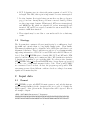
Figure 1: basic structure of a full-length LTR retrotransposon
The typical structure of a full-length LTR retrotransposon is shown in
Figure 1:
1. LTR Region: 5’LTR and 3’LTR are two similar regions. They are
identical while the element inserts into the host genome, and once inserted, they begin to evolve independently. Mutations and indels thus
are often found. A typical LTR retrotransposon has a structure called
TG..CA box, with TG at the 5’ extremity of 5’LTR and CA at the 3’
extremity of 3’LTR.
2. TSR Region: TSR(target site repeat) is a 4~6bp short direct repeat
string flanking the 5’ and 3’ extremities of an element. It is the sign of
insertion of transposable elements.
3. PBS: Near 3’ end of the 5’LTR, there is a ~18bp sequence complemented
to the 3’ tail of some tRNA. The site is very important because tRNA
binding process is the first step of initiating reverse transcription.
1
4. PPT: Polypurine tract is a short rich purine segment, about 11~15 bp
in length. Like PBS, this region is important for reverse transcription.
5. Protein domains: In a typical virus genome there are three polygenes:
gag, pol and env. Among them, pol is most conserved. Inside pol there
are three important domains: IN(integrase), RT(reverse transcriptase)
and RH(RNase H), which are enzymes for reverse transcription and
insertion. RT and IN are regarded essential for autonomous LTR elements to fulfill their function.
6. These signals may become blur or even undetectable for evolutionary
events.
1.2
Strategy
The Program first constructs all exact match pairs by a suffix-array based
algorithm and extends them to long highly similar pairs. Then SmithWaterman algorithm is used to adjust the ends of LTR pair candidates to get
alignment boundaries. These boundaries are subject to re-adjustment using
supporting information of TG..CA box and TSRs and reliable LTRs are selected. Next, LTR FINDER tries to identify PBS, PPT and RT inside LTR
pairs by build-in aligning and counting modules. RT identification includes
a dynamic programming to process frame shift. For other protein domains,
LTR FINDER calls ps scan (from PROSITE, http://www.expasy.org/prosite/)
to locate cores of important enzymes if they occur. Then possible ORFs
are constructed based on that. At last, the program reports possible LTR
retrotransposon models in different confidence levels according to how many
signals and domains they hit.
2
2.1
Input data
Format
LTR FINDER accepts only FASTA format sequences, and only the first ungapped string(identifier) in the description line is recorded to identify the
input sequence, other options in the description line will be ignored. Here is
an example of input:
>CHR1 19971009 Chromosome I Sequence
CCACACCACACCCACACACCCACACACCACACCACACACCACACCACACCCACACACACA
CATCCTAACACTACCCTAACACAGCCCTAATCTAACCCTGGCCAACCTGTCTCTCAACTT
2
ACCCTCCATTACCCTGCCTCCACTCGTTACCCTGTCCCATTCAACCATACCACTCCGAAC
... ... ... ...
TGATGGAGAGGGAGGGTAGTTGACATGGAGTTAGAATTGGGTCAGTGTTAGTGTTAGTGT
TAGTATTAGGGTGTGGTGTGTGGGTGTGGTGTGGGTGTGGGTGTGGGTGTGGGTGTGGGT
GTGGGTGTGGTGTGGTGTGTGGGTGTGGTGTGGGTGTGGTGTGTGTGGG
>CHR2 19970727 Chromosome II Sequence
AAATAGCCCTCATGTACGTCTCCTCCAAGCCCTGTTGTCTCTTACCCGGATGTTCAACCA
AAAGCTACTTACTACCTTTATTTTATGTTTACTTTTTATAGGTTGTCTTTTTATCCCACT
TCTTCGCACTTGTCTCTCGCTACTGCCGTGCAACAAACACTAAATCAAAACAATGAAATA
... ... ... ...
2.2
Size limit
Users could submit sequences large to 50,000,000 bytes. The timeout limit
for uploading sequence is 60 minutes. For users who want to scan very large
size sequences, executive binary code will be available on request.
3
Output format
LTR FINDER offers three types of output: Full output, Summary output
and Figure output.
3.1
Full output & Summary output
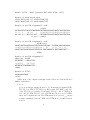
An example of Full output format is presented as follows:
>Sequence: CHR2 Len:813138
[1] CHR2 Len:813138
Location : 29632 - 35590 Len: 5959 Strand:+
Score
: 9 [LTR match score:1]
Status
: 11111111100
5’-LTR
: 29632 - 29963 Len: 332
3’-LTR
: 35259 - 35590 Len: 332
5’-TG
: TG , TG
3’-CA
: CA , CA
TSR
: 29627 - 29631 , 35591 - 35595 [ATAAT]
Sharpness: 0.479,0.52
Strand + :
PBS
: [17/22] 30031 - 30052 (ThrAGT)
PPT
: [11/15] 35215 - 35229
Domain: 31889 - 32416 [possible ORF:31193-35236, (IN (core))]
3
Domain: 33779 - 34387 [possible ORF:31193-35236, (RT)]
Details of exact match pairs:
35259-35472[214] (1) 35474-35590[117]
29632-29845[214] (1) 29847-29963[117]
Details of the LTR alignment(5’-end):
|35259
CATTAGATCTATTACATTATGGGTGGTATGTTGGAATAAAAATCAACTATCATCTACTAAC
|| || |
||| |||
|
|||*|||||||||||||||||||||||||||||
CA--AG--C----ACA-TAT-AAT----TGTTGGAATAAAAATCAACTATCATCTACTAAC
**-***----|29632
Details of the LTR alignment(3’-end):
35590|*****
ACAATTACATCAAAATCCACATTCTCTACAATAATAGAA--TAATGAA-CGATAACACACA
|||||||||||||||||||||||||||||* | |||
|| ||
|| | ||
ACAATTACATCAAAATCCACATTCTCTACA-TGGTAGCGCCTA-TGCTTCGGTTACTT--29963|
Details of the PBS alignment(+):
tRNA type: ThrAGT
GCTTCCAAT----CGG-ATTTG
|||||||||
||| |||||
GCTTCCAATTTACCGGAATTTG
|30031
Details of PPT(+):
AACAAACAAATGGAT
|35215
While most of the output is straight forward, there are some fields need
further explanation.
1. Score
Score is an integer varying from 0 to 11. It measures if signals (TSR,
TG..CA box, PBS, PPT, IN(core), IN(c-term), RT, RH) occur. Because TG..CA box consists of four parts: TG at 5’ end of 5’LTR, CA
at 3’ end of 5’LTR, TG at 5’ end of 3’LTR and CA at 3’ end of 3’LTR,
there are 11 signals in total. The LTR match score (matchscore ) is the
sequence similarity between 5’LTR and 3’LTR. It is a decimal between
0 and 1.
4
2. Status
Status is an 11 bits binary string, each bit indicates the status of a
certain signal. From left to right, signals are: TG in 5’ end of 5’LTR,
CA in 3’ end of 5’LTR, TG in 5’ end of 3’LTR, CA in 3’ end of 3’LTR,
TSR, PBS, PPT, RT, IN(core), IN(c-term) and RH. If a signal occurs,
corresponding position is 1 and 0 otherwise.
3. Sharpness
It is a decimal between 0 and 1 to evaluate the fineness of the boundary of LTR region. Higher sharpness means more accurate boundary
decision. The first value is sharpness of 5’ end and the second is that
of 3’ end. In a window of length 2W , Sharpness of the center position
is:
Minside Moutside
Sharpness =
−
W
W
where Minside and (Moutside ) are the number of matched bases in left
half and right half window respectively. Put the center position at the
LTR boundary to get the sharpness.
4. PBS & PPT
For PBS, the first number in square brackets is number of matched
bases and the second is total alignment length. For PPT, the first is the
number of purines and length of putative PPT. Following is signal positions. String in parentheses is the tRNA type and anti-codon(See this
web page for detail: http://lowelab.ucsc.edu/GtRNAdb/legend.html).
The minus sign before tRNA type stands for reverse strand(not showed
in this example).
5. Details of exact match pairs
This section shows the exact math pairs used to construct the LTR
alignment. Number in square brackets is the pair length and number
in parentheses is the distance between neighboring exact match pairs.
6. Details of the LTR alignment
This section shows the alignment details around 5’ and 3’ boundaries
of LTR regions. Single asterisk in ‘|’ line points out putative boundary
after the second run boundary decision (see Strategy Section). Other
4~6 continuous asterisks show the positions of putative TSR.
7. Details of PBS & PPT
Numbers indicates the 5’ ends of signals.
5
3.2
Summary output
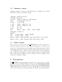
Summary output is extracted from Full-output by omitting some detailed
information. Here is an example output:
>Sequence: CHR2 Len:813138
[1] CHR2 Len:813138
Location : 29632 - 35590 Len: 5959 Strand:+
Score
: 9 [LTR match score:1]
Status
: 11111111100
5’-LTR
: 29632 - 29963 Len: 332
3’-LTR
: 35259 - 35590 Len: 332
5’-TG
: TG , TG
3’-CA
: CA , CA
TSR
: 29627 - 29631 , 35591 - 35595 [ATAAT]
Sharpness: 0.479,0.52
Strand + :
PBS
: [17/22] 30031 - 30052 (ThrAGT)
PPT
: [11/15] 35215 - 35229
Domain: 31889 - 32416 [possible ORF:31193-35236, (IN (core))]
Domain: 33779 - 34387 [possible ORF:31193-35236, (RT)]
3.3
Figure output
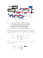
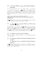
If user select output with figure, LTR FINDER will produce a PNG file to
show the relative position of each LTR retrotransposons. The figure was
plotted by both normal axis and logarithmic axis. Elements drawn on silver
background was plotted by their real size, that means, 1 pixel stand for 1
base. Elements drawn on white background was plotted under logarithmic
axis, so that the long distance could be resized to place on a small canvas.
Blue circles denote for PBS, brown circles stand for PPT, and purple circles
on the end of LTRs are TSRs.
4
Parameters
LTR FINDER has many parameters, which can be divided into two groups:
parameters used in finding LTR retrotransposons (construction parameters) and parameters used in filtering out unreliable results (filter parameters). The first group includes -o, -t, -e, -m, -u, -D, -d, -L, -l, -p, -g, -J,
-j, -s, -a and -r; the second group includes -S, -B, -b, -w, -O, -P and -F.
6
Figure 2: Legend of output figure
4.1
-o, Gap open penalty, (positive integer)
-t, Gap extend penalty, (positive integer)
-e, Gap end penalty, (positive integer)
-m, Match score, (positive integer)
-u, Mismatch score, (negative integer)
The five parameters control alignment algorithm. Denote gap open penalty
as Popen , gap extend penalty as Pext , gap end penalty as Pend , match score
as Smatch and mismatch score as Smismatch , then global and local alignments
score are :
Scorelocal = Smatch · Nmatch + Smismatch · Nmismatch
X
−
Pinner gap
Scoreglobal = Smatch · Nmatch + Smismatch · Nmismatch
X
−
Pinner gap − P50 gap − P30 gap
where Nmatch is the number of match bases; Nmismatch the number of unmatched bases; and
Pinner gap = Popen + Pext · (inner gap len − 1)
P50 gap = Pend · 50 gap len
P30 gap = Pend · 30 gap len
7
where inner gap len is the length of gap minus 2 (end bases). Usually, Popen
is greater than Smatch .
4.2
-D, Max distance between LTRs, (positive integer)
-d, Min distance between LTRs, (positive integer)
-L, Max LTR Length, (positive integer)
-l, Min LTR Length, (positive integer)
Distance between LTRs is:
Dist = P os30 LT R
begin
− P os50 LT R
end
+1
The four parameters makes detected models meet common features of LTR
retrotransposons.
4.3
-g, Extension max gap, (positive integer)
-j, Extension cutoff, (decimal between 0 and 1)
-J, Reliable extension, (decimal between 0 and 1)
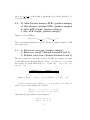
The three parameters control the extension of LTRs. An example of 2 neighbouring LTR pairs is shown in Figure 3. If s[ib . . . me ] and s[jb . . . ne ] are similar enough, we extend LTRs from s[ib . . . ie ] and s[mb . . . me ] to s[ib . . . me ]
and s[jb . . . ne ].
ib
ie
jb
mb
je
me
nb
ne
Figure 3: P1 {s[ib . . . ie ], s[jb . . . je ]} and P2 {s[mb . . . me ], s[nb . . . ne ]}
P1 and P2 are pre-sorted so that jb ≥ ib , nb ≥ mb and jb ≥ mb . Since P1
and P2 are two exact match pairs, we know
lenpair1 =
ie − ib + 1 = j e − jb + 1
lenpair2 = me − mb + 1 = ne − nb + 1
Obviously, the gap lengthes between them are
gap1 = mb − ie − 1
gap2 = nb − je − 1
8
Introduce Dif f , number of base differences resulting from extension, as
Dif f =
(
Lengthinner mis
gap1 > 0 and gap2 > 0
max{gap1 , gap2 } − min{gap1 , gap2 } otherwise
where Lengthinner mis is the number of different(mismatches and indels) bases
from global alignment of s[ie + 1 . . . mb − 1] and s[je + 1 . . . nb − 1]. The
similarity of merged loci is then:
Sim =
lenpair1 + max{gap1 , gap2 } + lenpair2 − Dif f
lenpair1 + max{gap1 , gap2 } + lenpair2
When LTR FINDER decides whether two neighboring pairs should be
merged, it first calculates Dif f , make sure that it does not exceed the value
of extension max gap, then calculates Sim. If Sim < extension cutof f ,
pair extension will stop here, P1 {s[ib . . . ie ], s[jb . . . je ]} will be reported as a
candidate for LTR element; If Sim > reliable extension, new pair P2 and
inter-pair regions will be linked to the previous one P1 to construct a longer
new pair P {s[ib . . . me ], s[jb . . . ne ]}, and LTR FINDER continues to find next
neighboring pairs; if extension cutof f < Sim < reliable extension, it means
we are not sure whether continue to extend or stop. So LTR FINDER first
report a LTR element candidate P1 {s[ib . . . ie ], s[jb . . . je ]} while at the same
time, the extension process will continue.
4.4
-p, Length of exact match pairs, (positive integer)
Running time of LTR FINDER is very sensitive to this parameter. The
program only selects pairs that are longer than this value to do further processes from all exact match pairs detected. If a very small value is given,
LTR FINDER will spend much time on randomly matched short sequences.
We use P-value to estimate proper value of -p, that is, the probability of exact match of length longer than L occurs if 2 sequences are drown randomly.
In Waterman 1989(?), under independent letter model, using asymptotic extreme value distribution, P-value were worked out analytically. Now if one
assign the P-value, length can be deduced. From experiments, 20 is appropriate in most situation, and we suggest not using of value less than 15.
4.5
-r, Min match length for PBS detection, (positive
integer)
When aligning tRNA 3’ tail 18nt string to the inter-LTR sequence, if LTR FINDER
finds an alignment that match length exceeds this threshold, it will report
this region as a putative primer binding site.
9
4.6
-s, Predict PBS by using which tRNA database,
(filename)
To predict primer binding site, we need tRNA sequences, especially the
3’ end 18nt of each sequences. LTR FINDER can load tRNA of different species. A good tRNA set can be found at Genomic tRNA Database
(http://lowelab.ucsc.edu/GtRNAdb/). Our database was download from
Genomic tRNA Database on 2007-07-17. Here is an example of required
format:
>Athal-chr4.trna25-AlaAGC (13454563-13454635)
GGGGATGTAGCTCAGATGGTAGAGCGCTCGCTTAGCATGCGAGAGGCACGGGGATCGATA
CCCCGCATCTCCA
LTR FINDER uses the string after the last minus sign in sequence identifier
field as the tRNA type name. In this example, ‘AlaAGC’.
4.7
-a, Use ps scan to predict IN(core), IN(c-term)
and RH, dirname
This parameter is a directory name. LTR FINDER can predict protein domains by calling ps scan, which can be obtained from ExPASy-PROSITE
(http://www.expasy.org/prosite/). User should place data file ‘prosite.dat’
and ps scan in this directory. If this parameter is enabled, LTR FINDER
will call them and report these protein domains if they are detected.
4.8
-S, Output score threshold, (integer)
This is the threshold for LTR retrotransposon score. Models that have higher
scores are output.
4.9
-B, Sharpness higher threshold, (decimal between
0 and 1)
-b, Sharpness lower threshold, (decimal between
0 and 1)
LTR FINDER calculates sharpness for both 5’ and 3’ extremities of putative
elements. Both of them must be greater than the lower threshold and one
greater than the higher threshold.
10
4.10
-w, Output format, (0,1 or 2)
This parameter controls the output format:
Value
0
1
2
4.11
Format
Full output
Summary output
Table output(not available on web)
-O, Length of alignment details, (positive integer)
LTR FINDER can output alignment details of LTR boundaries (left to 120bp
and right to 80bp relative to boundaries). Users are allowed to assign the
output length by setting this parameter. The whole 200 bp alignment is
output when it ≥ 120.
4.12
-P, Sequence ID pattern, (POSIX regular expression)
This parameter is ID of one sequence in a multi-fasta file. When enabled,
only sequences with this ID will be processed.
4.13
-F, Signals status control, (01 string)
The parameter controls output by sequence tag status. It is a binary string
of 11 bits. From left to right, bits denote the status of following signals:
TG in 5’ end of 5’LTR, CA in 3’ end of 5’LTR, TG in 5’ end of 3’LTR, CA
in 3’ end of 3’LTR, TSR, PBS, PPT, RT, IN(core), IN(c-term) and RH. 1
means reported models should containing the signal and 0 ignoring searching
it. when used, the program will only report models whose status of sequence
tags match it.
4.14
-C, Auto mask highly repeated regions
With this parameter, LTR FINDER will try to mask highly repeated regions
defined by: the same exact match pair repeat 14 more times within 3000bp.
By using this parameter, LTR FINDER can perform much more quickly on
sequences which have centriole or telomere region.
11
5
Acknowledgements
We thank Heng Li for his linear-space pairwise alignment library and Xiaoli
Shi for providing rice tRNA sequences. The authors are also grateful to
colleagues who helped us testing the web server.
References
Flavell, R. B. (1986). Repetitive dna and chromosome evolution in plants. Philos Trans R Soc Lond B Biol
Sci, 312(1154), 227–242.
Gao, L., McCarthy, E. M., Ganko, E. W., and McDonald, J. F. (2004). Evolutionary history of oryza sativa ltr
retrotransposons: a preliminary survey of the rice genome sequences. BMC Genomics, 5(1), 18.
Gao, X., Havecker, E. R., Baranov, P. V., Atkins, J. F., and Voytas, D. F. (2003). Translational recoding signals
between gag and pol in diverse ltr retrotransposons. RNA, 9(12), 1422–1430.
Jordan, I. K. and McDonald, J. F. (1998). Evidence for the role of recombination in the regulatory evolution of
saccharomyces cerevisiae ty elements. J Mol Evol, 47(1), 14–20.
Kalyanaraman, A. and Aluru, S. (2006). Efficient algorithms and software for detection of full-length ltr retrotransposons. J Bioinform Comput Biol, 4(2), 197–216.
Kim, J. M., Vanguri, S., Boeke, J. D., Gabriel, A., and Voytas, D. F. (1998). Transposable elements and genome
organization: a comprehensive survey of retrotransposons revealed by the complete saccharomyces cerevisiae
genome sequence. Genome Res, 8(5), 464–478.
Ma, J., Devos, K. M., and Bennetzen, J. L. (2004). Analyses of ltr-retrotransposon structures reveal recent and
rapid genomic dna loss in rice. Genome Res, 14(5), 860–869.
McCarthy, E. M. and McDonald, J. F. (2003). Ltr struc: a novel search and identification program for ltr
retrotransposons. Bioinformatics, 19(3), 362–367.
McCarthy, E. M. and McDonald, J. F. (2004). Long terminal repeat retrotransposons of mus musculus. Genome
Biol, 5(3), R14.
McCarthy, E. M., Liu, J., Lizhi, G., and McDonald, J. F. (2002). Long terminal repeat retrotransposons of oryza
sativa. Genome Biol, 3(10), RESEARCH0053.
McDonald, J. F. (1993). Evolution and consequences of transposable elements. Curr Opin Genet Dev , 3(6),
855–864.
McDonald, J. F., Matyunina, L. V., Wilson, S., Jordan, I. K., Bowen, N. J., and Miller, W. J. (1997). Ltr
retrotransposons and the evolution of eukaryotic enhancers. Genetica, 100(1-3), 3–13.
SanMiguel, P., Tikhonov, A., Jin, Y. K., Motchoulskaia, N., Zakharov, D., Melake-Berhan, A., Springer, P. S.,
Edwards, K. J., Lee, M., Avramova, Z., and Bennetzen, J. L. (1996). Nested retrotransposons in the intergenic
regions of the maize genome. Science, 274(5288), 765–768.
Xiong, Y. and Eickbush, T. H. (1990). Origin and evolution of retroelements based upon their reverse transcriptase sequences. EMBO J , 9(10), 3353–3362.
Yoder, J. A., Walsh, C. P., and Bestor, T. H. (1997). Cytosine methylation and the ecology of intragenomic
parasites. Trends Genet, 13(8), 335–340.
Zhang, X. and Wessler, S. R. (2004). Genome-wide comparative analysis of the transposable elements in the
related species arabidopsis thaliana and brassica oleracea. Proc Natl Acad Sci U S A, 101(15), 5589–5594.
12