Download USER MANUAL OF UNF CODE - International Atomic Energy Agency

CNIC-01616
CNDC-0032
USER MANUAL OF UNF CODE
ZHANG Jingshang
China Nuclear Data Centre
China Nuclear Information Centre
China Nuclear Industry Audio & Visual Publishing House
Contents
Introduction ………………………………………………………(1)
1 Spherical Optical Potential………………………………………(3)
2 Parameters of UNF Code ………………………………………(6)
3 Flags ……………………………………………………………(7)
4 Input Files ………………………………………………………(7)
5 Output Files ……………………………………………………(13)
6 Guide for Running UNF Code…………………………………(14)
Appendix A ………………………………………………………(17)
n+0Cu sample input files of “UNF.DAT”……………………(17)
n+0Cu sample input files of “DIR.DAT” ……………………(25)
n+0Cu sample input files of “OTH.DAT” ……………………(30)
Appendix B: UNF Code for Fast Neutron Reaction
Data Calculations…………………………………………………(31)
Reference…………………………………………………………(58)
Introduction
The UNF code (2001 version) written in FORTRAN-90 is developed for
calculating fast neutron reaction data of structure materials with incident energies
from about 1 keV up to 20 MeV. There are 87 subroutines and 15 functions in
UNF code.
The code consists of the spherical optical model, the unified HauserFeshbach and exciton model. The angular momentum dependent exciton model
is established to describe the emissions from compound nucleus to the discrete
levels of the residual nuclei in pre-equilibrium processes, while the equilibrium
processes are described by the Hauser-Feshbach model with width fluctuation
correction. The emissions to the discrete level in the multi-particle emissions for
all opened channels are included. The double-differential cross sections of
neutron and proton are calculated by the linear momentum dependent exciton
state density. Since the improved pickup mechanism has been employed based
on the Iwamoto-Harada model, the double-differential cross sections of alphaparticle, 3He, deuteron and triton can be calculated by using a new method based
on the Fermi gas model. The recoil effects in multi-particle emissions from
continuum state to discrete level as well as from continuum to continuum state
are taken into account strictly, so the energy balance is held accurately in every
reaction channels. If the calculated direct inelastic scattering data and the
calculated direct reaction data of the outgoing charged particles are available
from other codes, one can input them, so that the calculated results will included
the effects of the direct reaction processes. To keep the energy balance, the recoil
effects are taken into account for all of the reaction processes. The gammaproduction data are also calculated. The calculated neutron reaction data can be
output in the ENDF/B-6 format.
All formulation used in UNF code can be found in the book entitled
1
“NEUTRON PHYSICS——Principle, Method and Application” published by
China Atomic Energy Press in 2001.
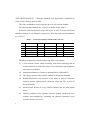
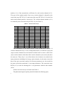
The code can handle a decay sequence up to (n,3n) reaction channel.
The total reaction channels are 14 (0:13) as shown in the Table 1.
In fact the reaction channels (n,np) and (n,pn) as well as (n,nα) and (n,αn)
should be treated as one channel, respectively. Thus the total reaction channels
are 12 (0:11).
Table 1 14 reaction channels considered in UNF code
No.
Channels
No.
Channels
No.
Channels
0
n,γ
(n,n')
5
(n,d)
10
(n,pn)
6
(n,t)
11
(n,2p)
7
8
(n,2n)
(n,np)
12
13
(n,αn)
(n,3n)
9
(n,nα)
1
2
3
4
(n,p)
(n,α)
(n,3He)
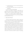
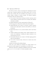
The physical quantities calculated by using UNF code contain:
(1) Cross sections of total, elastic scattering, non-elastic scattering, and all
reaction channels in which the discrete level emissions and continuum
emissions are included.
(2) Angular distributions of elastic scattering both in CMS and LS.
(3) The energy spectra of the particle emitted in all reaction channels.
(4) Double-differential cross sections of all kinds of particle emissions
(neutron, proton, alpha-particle, deuteron, triton and 3He, as well as
the recoil nuclei.
(5) Partial kerma factors of every reaction channel and the total kerma
factor.
(6)
Gamma production data (gamma spectra, gamma production cross
sections and multiplicity), including the gamma production cross
sections from level to level.
2
(7) Total double-differential cross sections of each kind outgoing particles
from all reaction channels.
(8) Cross sections of isomeric states, if the level is a isomeric state of the
residual nucleus.
(9) dpa cross sections used in radiation damage.
UNF code can also handle the calculations for a single element or for
natural nucleus, and the target can be in ground state or in its isomeric state.
Besides the output file, the outputting in ENDF/B-6 format is also included
(files3, 4, 6, 12, 13, 14, 15 or files-3, 4, 5, which are controlled by a flag).
Meanwhile, some self-checking functions are designed for checking the
errors in the input parameter data, if it exist. Users can correct them according to
the indicating information in advance.
1 Spherical Optical Potential
In UNF code the spherical optical potential is employed to calculate total
cross section, shape elastic scattering cross section and its angular distribution,
absorption cross section, as well as the transmission coefficients and inverse
cross section of the reaction channels No: 1-6 for (n,p, α, 3He, d, t).
For the reaction channels (n,2n) and (n,3n) the transmission coefficients are
taken from (n,n) channel. The calculated transmission coefficients for the second
emitted particles of the reaction channels (n,pn), (n,pp), and (n,αn) with the same
parameters as that for these particles in the channels No: 1-2, but with different
mass number and charge number, accordingly. The transmission coefficients of p
and α in the reaction channels (n,np) and (n,nα) are taken from (n,p) and (n,α)
channels, respectively. Therefore 9 sets of the transmission coefficients are
needed to be calculated. Some conversion arrays are used in the UNF code to
mark the data. The conversion array KOP (0:13) denotes the corresponding
3
number (1:9) of the transmission coefficients for each reaction channel (0:13).
The type of the emitted particle from every reaction channel is denoted by the
conversion array KTYP1 (0:13) and conversion array KTYP2 (0:13) for the first
and second emitted particles, respectively. The reaction channel number (0:11)
are marked by the conversion array KCH (0:13) (See Table 2).
Table 2 14 conversion arrays
No.
0
1
Channels
(n,γ)
(n,n')
KOP
KTYP1
0
KTYP2
0
KGD
0
KCH
0
1
1
1
1
1
2
(n,p)
2
2
2
2
2
3
3
3
3
3
3
4
(n,α)
(n,3He)
4
4
4
4
4
5
(n,d)
5
5
5
5
5
6
(n,t)
6
6
6
6
6
7
(n,2n)
1
1
1
7
7
8
(n,np)
2
1
2
5
8
9
3
1
3
8
9
10
(n,nα)
(n,pn)
7
2
1
5
8
11
(n,2p)
8
2
2
9
10
12
(n,αn)
(n,3n)
9
3
1
8
9
1
1
1
10
11
13
The construction of the discrete levels of the residual nuclei for the 14
reaction channels has only 11 sets of independent nuclei, of which the (n,np) and
(n,pn) reaction channels have the identical residual nuclei as same as that of the
(n,d) reaction channel, while that of the reaction channels (n,nα) and (n,αn) have
the same one. Thus, only 11 sets of the discrete level schemes are needed in the
input parameters including level energy, spin and parity. As the same reason, the
data of the pair corrections and the level density parameters are also needed as
the same as the afore-mentioned 11 sets input parameters. The conversion array
KGD (0:13) is used for denoting the 11 sets parameters with the order number
(0:10).
All the conversion arrays are listed in the Table 2 .
The phenomenological optical potential includes the following parts;
4
(a): Real part
Vr ( r ) =
− Vr (ε )
1 + exp[( R − rr ) / a r ]
(b): Imaginary part of surface absorption
Ws (r ) = −4Ws (ε )
exp[(r − Rs ) / as ]
(1 + exp[(r − Rs ) / as ]) 2
(c): Imaginary part of volume absorption
Wv ( r ) =
− U v (ε )
1 + exp[(r − Rv ) / a v ]
(d): Spin-orbit potential
Vso (r ) = −
2Vso
exp[(r − Rso ) / aso ]
aso r (1 + exp[(r − Rso ) / aso ]) 2
(e): Coulomb potential
ZbZ
r2

0.7720448 R (3 − R 2 )
c
c
Vc ( r ) = 
1.440975 Z b Z

r
if r ≤ Rc
if r > Rc
where A, Z stand for the mass and charge numbers of target nucleus, sb and
Zb are the spin and charge number of particle b and ε is the energy of particle b in
the center of mass system.
The total optical potential reads
Vb(r)= Vr(r)+i[Ws(r)+Wv(r)]+Vso(r)+Vc(r)
The energy dependence of potential depths are given by
Vr(ε)=V0+V1ε+ V2ε2+V3(A-2Z)/A+V4(Z/ A1/3)
Ws(ε)=W0+W1ε+W2(A-2Z)/A
Uv(ε)=max {0., U 0 + U 1ε + U 2 ε 2 }
5
All kinds of radius are given by
Ri=riA1/3
(i=r, s, v, so, c)
In particular the diffusion widths of imaginary potential for proton take the
form
a s = a s 0 + a s1
A − 2Z
A
a v = a v0 + a v1
A − 2Z
A
Thus, altogether there are 12 parameters for potential depth, 5 parameters
for radiuses and 4 (or 6 for proton) for diffusion widths in the phenomenological
optical potential.
2 Parameters of UNF Code
There are three parameters in UNF code to control the storage size.
NEL: (integer) is the permitted maximum number of incident energy points.
NLV: (integer) is the permitted maximum number of the discrete levels
including the ground state of the compound nucleus and the residual
nuclei of the reaction channel No:1-6. The permitted maximum
number is fixed 20 for the residual nuclei of the reaction channels
No:7-11.
NGS: (integer) is the permitted maximum bin number of the γ production
spectra.
So far the values of the three parameters in UNF code are set NEL=250,
NLV=40, and NGS=300, respectively. If the users want to increase the size, then
change the value accordingly, and compile the code again.
6
3 Flags
In UNF code several flags were set for different calculation purpose, so that
the users should understand the functions of these flags in advance.
(1) KTEST: if users want to study some medium results for physical
analysis, then set KTEST=1, when doing the calculation of multiincident energy points users would be better to set KTEST=0,
otherwise the output size may be too large.
(2) KOPP: if users want to output the optical potential parameters then set
KOPP=1, otherwise set KOPP=0.
(3) KDDCS: It is used to control the double-differential cross section
calculations. When user only want to calculate the data of the reaction
cross sections, then set KDDCS=0, while user needs the data of the
double-differential cross sections, then set KDDCS=1.
(4) KGYD: It is used to control the γ-production calculation. When users do
not need them, then set KGYD=0, otherwise set KGYD=1.
(5) KENDF: It is used to control the ENDF/B-6 format output. In general
the physical results are output in the file ''UNF.OUT''. When users need
the ENDF/B-6 format outputting, then set KENDF=1 for the files-3, 4,
6, 12, 13, 14, 15 outputting, and set KENDF=2 for only the files 3, 4, 5,
otherwise set KENDF=0 without ENDF/B-6 format outputting.
4 Input Files
Three input files are set up in UNF code.
4.1 File “UNF.DAT”
(A) For the common used parameters. The sequence of the input data is
illustrated as below:
Card 1: The 5 flags are input with the sequence as same as that mentioned
7
above, which are KTEST, KOPP, KDDCS, KGYD, KENDF.
Card 2: The status of target KS0 (Integer) KS0=1 for ground state, KS0>1
for isomeric state (the number is the level order number, here the
ground state is 1)
Card 3: NAB (Integer) is the number of isotopes, NAB=1 only for one
isotope, while NAB>1 for natural nucleus. So far NAB≤10 is
limited in UNF code.
Card 4: IZT(Integer) Charge number of target
Card 5: IAT(1:NAB) (Integer) The mass numbers of each isotope
Card 6: FONG(1:NAB) (Real) The abundance of each isotope
Card 7: MAT (Integer) Material number to mark the element in ENDF/B-6
format file
Card 8: MEL: (Integer) Number of incident energies and NOE: (Integer)
(notation: NOE=0 Doing the calculation for all incident energies; NOE≠0
Only doing the calculation for single incident energies with the order
number NOE (1≤NOE≤MEL) )
EL(I), I=1, MEL(real) incident energies in unit of MeV
MET(I), I=1, MEL(integer) energy point type
MET(I)=1 only output cross sections
MET(I)=2 output cross sections and angular distributions
MET(I)=3 besides outputting cross sections and angular
distributions, the outputting double-differential cross section
and γ production data is also issued in ENDF/B-6 format.
Card 9: The 5 angels for the neutron double-differential cross sections
outputting to fit the measured data in laboratory system.
Card 10: DLH (real) Bin size of γ spectra.
(B) For each isotope the input data are as follows:
8
The sequence of the input data is illustrated as below
Card 1:
AMT (real) mass of the target in unit of a.m.u
CK (real) Kulbach parameter in exciton model
EF (real) Fermi energy (MeV)
CE1 (real) adjustable factor in γ radiation
Card 2:
EHF: (real) The energy bound between the Hauser-Feshbach model
and the unified Hauser-Feshbach and exciton model.
If EL(LE) < EHF the Hauser-Feshbach model is used;
If EL(LE) > EHF the pre-equilibrium reaction model is performed.
Card 3:
BIND(0:13) (real) Binding energies of the last emitted particle of the
reaction channels (0:13) (Notation: BIND(0)=0. for gamma
emission)
ALD(0:10) (real) Level density parameters of the 11 residual nuclei
( Gilbert-Cammeron formula is employed in UNF code)
DELT(0:10) (real) Pair correction values of 11 residual nuclei
Card 4: Two peak giant resonance parameter used for Gamma emissions
CSGA (0:10,1:2) absorption cross sections of photo-nuclear
reactions for 11 residual nuclei (in b)
EG(0:10,1:2) Energies of two peak giant dipole-resonance for 11
residual nuclei.(in MeV)
GG(0:10,1:2) Widths of giant dipole-resonance peaks (in MeV). The
input sequence is CSGA(I,1), CSGA(I,2), EG(I,1), EG(I,2),
GG(I,1), GG(I,2), I=0:10
Card 5: DGM (real) The parameter of the direct gamma emission
Card 6: Data of the discrete levels
9
NDL(0,10) (integer) Number of discrete levels of residual nuclei
EDL(0:10,K) (real) K=1, NDL(I) Level energies in unit of MeV
SDL(0:10,K) (real) K=1, NDL(I) Spins of levels
IPD (0:10,K) (integer) K=1, NDL(I) Parities of levels (+1 or -1). The
input sequence is NDL(I), I=0,10
J=0:10 for (n,γ), (n,n'), (n,p), (n,α), (n,3He), (n,d), (n,t), (n,2n), (n,nα),
(n,2p), and (n,3n) reaction channels.
EDL(J,K), K=1, NDL(J)
SDL(J,K), K=1, NDL(J)
IPD(J,K), K=1, NDL(J)
(Notation: the order number of the ground state is 1, the order number
of the first excitation level is 2 and so on. If NDL(I)=0, then the
content of the J=I term is empty)
Notations 1: for calculation of natural nucleus, limited by ENDF/B-6
format, the total number of the discrete levels included in all
isotopes of the inelastic scattering channel could no be over 40,
if user want to set up the data file in ENDF/B-6 format.
Notations 2: for the reaction channels of multi-particle emissions,
such as (n,np), (n,pn), (n,nα), (n,αn), (n,2p) and (n,3n), the
number of discrete levels could not be over 20 in the calculation
limited by UNF code. Since the number of reaction channel (n,d)
has identical residual nucleus with (n,np) and (n,pn), so the
number of discrete levels could also not be over 20.
Card 7: Branching ratio in γ de-excitation process. The branching ratio from
Ith level to Jth level is written in the format (I3, I3, F5.2). The
number of the lines of the input branching ratios for each
residual nucleus is denoted by NUL (integer). Thus, the input
order for each residual nucleus is NUL (integer) 6(I3, I3, F5.2)....
10
NUL lines.
There are 6 set data in one line. If the branching ratio between two
levels is 0, then it does not need in the input file.
The input sequence is J=0:10 for (n,γ), (n,n'), (n,p), (n,3He), (n,d),
(n,t), (n,2n), (n,nα), (n,2p) and (n,3n) reaction channels.
Card 8: Optical potential parameters
AR Array (1:6). Diffusivities parameters of real potentials
AS Array (1:6). Diffusivities of sur. abs. ima. potentials
AVV Array (1:6). Diffusivities of volume absor. imag. potentials
AS0 Array (1:6). Diffusivities of L-S coupling potentials
XR Array (1:6). Radius parameters of real potentials
XS Array (1:6). Radiuses of sur. abs. ima. potentials
XV Array (1:6). Radiuses of volume absor. imag. potentials
XS0 Array (1:6). Radiuses of L-S coupling potentials
XC Array (1:6). Coulomb potentials Radius parameters
U0 Array (1:6). Constant terms of volume absorption imaginary
potentials
U1 Array (1:6). Energy-linear term factors of volume absorption
imaginary potentials
U2 Array (1:6). Energy-square term factors of volume absorption
imaginary potentials
V0 Array (1:6). Constant factors in real potential for x particle of
(n,x) reactions, with x=n,p, 3He, d, t.
V1 Array (1:6). Energy-linear term factors in real potentials
V2 Array (1:6). Energy-square term factors in real potentials
V3 Array (1:6). Charge-symmetry term factors in real potentials
V4 Array (1:6). Charge-linear term factors in real potentials
VS0 Array (1:6). Constant factors of L-S coupling potentials
11
W0 Array (1:6). Constant terms of surface absorption imaginary
potentials
W1 Array (1:6). Energy-linear term factors of surface absorption
imaginary potentials
W2 Array (1:6). Charge-symmetry term factors of surface
absorption imaginary potentials
A2S AS(proton) =AS(2) + A2S. (N-Z)/A only for proton
A2V AVV(proton) =AVV(2) + A2V. (N-Z)/A only for proton
In the case of natural nucleus the more isotopes (NAB>1) are
needed to be calculated, the input parameters of the second
isotope should be given in the same format as the first isotope.
Then the ENDF/B-6 outputting is given for the natural nucleus.
4.2 File “DIR.DAT”: This file is used for inputting the data of direct inelastic
scattering and direct reactions, the input sequence is
I=1 direct inelastic scattering
I=2 direct reaction of (n,p)
I=3 direct reaction of (n,α)
I=4 direct reaction of (n,3He)
I=5 direct reaction of (n,d)
I=6 direct reaction of (n,t)
In Ith term the input order is that the first line is the channel explanatory note,
the second line gives the values of NPE (the number of incident energies, so far
NPE≤40 is limited in UNF code) and LDM (the maximum value of the angular
momentum in Legendre expansion form, LDM≤20 is limited in UNF code), the
third line gives NDL(I) integers with 1 or 0, while “1” or “0” means the direct
process is taken or is not taken into account for the level. In each incident energy
input the cross section CSDIR(K) and the Legendre coefficients FL(0:LDM, K)
of the level with the integer “1” in the array NDL.
12
4.3 File “OTH.DAT”
Card 1: If the user wants to observe the γ production data between levels,
then set this file as follows:
For each kind of residual nuclei (0:10), at first input a integer NGM,
which implies the number of the observed γ ray production between
levels by user. Then input NGM pair integer of the level order
numbers in this residual nucleus. For each integer pair (k1, k2)
implies the γ ray is emitted from k1 level to k2 level, (so k1>k2). If
the user does not want to observe this term, then set a “0” in this
residual nuclei.
Card 2: If the user wants to calculate the reaction cross sections of the
isomeric level within the 11 kind of residual nuclei (0:10), then set
the isomeric level number in this residual nucleus, otherwise only
set “0” in it.
Card 3: If set KDPA=1 the dpa cross sections will be calculated, otherwise
set KDPA=0.
Card 4: Input the threshold energy Ed of PKA in unit of MeV.
This file only used for NAB=1 for one element calculation. But in
the case of NAB>1 the NAB elements data for OTH.DAT are
needed since different element may have different status of isomeric
level.
5 Output Files
Five files are opened in UNF code for outputting
(1) File “UNF.OUT” This file is used for the output of calculated quantities
(2) File “PLO.OUT” This file is used for the DDCS outputting of all kinds
outgoing particles, as well as the angular-energy spectra of 5 angles for
13
outgoing neutron in laboratory system when NOE>0.
(3) File “B6.OUT” This file is used for outputting the file in ENDF/B-6
format if KENDF=1 or 2.
(4) File “KMA.OUT” This file is used for outputting kerma factors.
(5) File “DPA.OUT” This file is used for outputting the dpa cross sections if
KDPA=1 in the ODH.DAT file.
6 Guide for Running UNF Code
In order to calculate the fast neutron data, some preparations need to be set
down in advance.
(1) At first set the UNF.DAT file.
(2)
If the data of the direct inelastic scattering and direct reaction are
available from other codes, then input the data in the file “DIR.DAT”
with the proper format (See 4.2). If Ith direct reaction data are not
taken into account, the user must put a “0” in this channel of file
“DIR.DAT”.
(3)
Set the OTH.DAT in advance. After set down the preparations
mentioned above, the users can start the neutron data calculation.
(4) After adjustment procedure of parameters, users set KENDF=1 (in
general KTEST=0) and run UNF code. The physical results output in
file “UNF.OUT” and the ENDF/B-6 output in file “B6.OUT”.
(5)
If the running is stop, and some information occurs on the screen,
which informs the user there are some errors in the input data file,
then the user needs to correct them accordingly.
(6) When set KTST=1 and NOE>0 for performing one incident neutron
energy calculation, the threshold energies of every reaction channels,
as well as that of inelastic scattering of the discrete levels are given in
14
“UNF.OUT” file, which are useful for the calculation to set up the
ENDF/B-6 outputting file. Meanwhile, checking the normalization of
the de-excitation ratios, some other information will be given to make
sure that the input data file are (or not) correct.
(7) Only in the case of NOE>0 for one incident energy point calculation,
the 5 set of double-differential cross sections will be output in
“PLO.OUT” file for fitting the measured data.
Notations: In the input files “UNF.DAT” and “DIR.DAT” there are some
one-line-annotations to indicate the data contents. UNF code reads them as a
character. So the users must pay attention to ''do not leaving any space lines
ahead these characters'' when writing at the input data. Otherwise all of the
reading must be out of order.
An interface “PRE-UNF” based on RIPL has been established to set up the
UNF.DAT and OTH.DAT files mentioned above automatically. If NAB>1 the
NAB elements for each element with the charged number of Z can be set up
simultaneously for both UNF.DAT file and OTH.DAT file, so the user needs to
pay attention to whether any isomeric level is involved in a element.
15
16
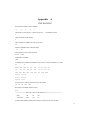
Appendix A
UNF.DAT FILE
KTEST KOPP KDDCS KGYD KENDF
0
0
1
1
1
THE STATUS OF TARGET 1: GROUND STATE
>1: ISOMERIC STATE
1
THE NUMVER OF ISOTOPES
2
THE CHARGE NUMBER OF THE NUECLEUS
29
MASS NUMBERS OF EACH ISOTOPES
63
65
ABUNDANCE OF EACH ISOTOPES
0.6917
0.3083
MATERIAL NUMBER
3290
NUMBER OF INCIDENT ENERGIES, 'NOE','EL(I),I=1,MEL AND MET(I),I=1,MEL
29
0
0.001 0.01
0.05
0.1
0.5
0.75
1.0 1.5 2.0
2.5
3.0
4.0
4.5
5.0
6.0
7.0 7.5 8.0
9.0
15.0
16.0 17.5 18.0
10.0
3.5
12.0 14.0 14.5
20.0
31121 13122
21312 32131
33312 3133
ANGLES IN LS FOR FITTING DDCS OF NEUTRON
30. 60. 90.
120. 150.
BIN SIZE IN GAMMA PRODUCTION
0.10
============= THE INPUT DAT OF ELEMENT No:1 ==================
M(T)
62.9295898
CK
EF
CE1
500.0
32.0
1.0
ENERGY BOUND BETWEEN HF AND MULTI-STEP REACTION MODEL
17
6.5
BINDING ENERGIES(0:13)
0.0
7.9160919 7.1995635
6.2011445
17.444110
11.816096 16.155116
10.854230 6.1246310 5.7765668
6.8411410
11.275454
7.4915142 8.8941669
LEVEL DENSITY PARAMETERS(0:10)
7.765, 7.161, 7.455, 7.754, 8.195, 7.336, 7.857, 6.731, 7.199, 8.804, 6.182,
PAIR CORRECTION VALUES(0:10)
-0.18, 1.3, 2.5, -0.25, 1.2, 2.5, 1.05, -0.15, 1.22, -0.28, 1.32,
PARAMETERS OF GIANT RESONANSE MODEL(CSE EE GG) (0:10)
0.075, 0.075, 0.034, 0.026, 0.026, 0.034, 0.034, 0.075, 0.026, 0.026, 0.075,
0.0, 0.0,
0.050, 0.040, 0.040, 0.050, 0.050, 0.0,
0.040, 0.040, 0.0,
16.70,16.70, 16.30, 16.37, 16.37, 16.30, 16.30, 16.70, 16.37, 16.37,16.70,
16.70,16.70, 16.30, 16.37, 16.37, 16.30, 16.30, 16.70, 16.37, 16.37,16.70,
0.0, 0.0,
18.51, 18.90, 18.90, 18.51, 18.51, 0.0, 18.90, 18.90, 0.0,
6.89, 6.89, 2.44, 2.56, 2.56,
2.44, 2.44,
6.89, 2.56,
2.56,
6.89,
PARAMETER OF DIRRECT GAMMA (DGAM)
0.25
DISCRETE LEVEL NUMBER FOR ALL RESIDUAL NUCLEI No:1
11, 18, 0, 0, 0, 0, 0, 8, 9, 0, 9,
FOR(N,G) 64-CU
0.0, 0.1593, 0.2783, 0.3439, 0.3622, 0.5746, 0.6088, 0.6630, 0.7391, 0.7462, 0.8783,
1.0, 2.0,
2.0,
1.0,
3.0,
4.0,
2.0,
1.0,
2.0,
3.0,
0.0,
11*1,
FOR (N,N) 63-CU
0.0,
0.6697, 0.9621, 1.3270, 1.4120, 1.5470, 1.8612, 2.0112, 2.0622, 2.0814,
2.0926, 2.2079, 2.3366, 2.3380, 2.4048, 2.4972, 2.5064, 2.5120,
1.5,
0.5,
2.5,
3.5,
2.5,
1.5,
3.5,
1.5,
3.5,
0.5,
2.5,
1.5,
3.5,
1.5,
4.5,
0.5,
13*-1, 1, -1, -1, 1, -1,
FOR (N,P) 63-Ni
FOR (N,A) 60-Co
FOR (N,He) 61-Co
FOR (N,D) 62-Ni
FOR (N,T) 61-Ni
18
0.5,
2.5,
FOR (N,2N)) 62-CU
0.0, 0.0408, 0.2435, 0.2878, 0.3902, 0.4261, 0.5483, 0.6375,
1.0, 2.0,
2.0,
2.0,
4.0,
3.0,
1.0,
1.0,
8*1,
FOR (N,NA) 59-Co
0.0, 1.0993, 1.1905, 1.2916, 1.4343, 1.4595, 1.4817, 1.7447, 2.0618,
3.5, 1.5,
4.5,
1.5,
0.5,
5.5,
2.5,
3.5,
3.5,
9*-1,
FOR (N,2P) 62-Co
FOR (N,3N) 61-CU
0.0, 0.4751, 0.9701, 1.3106, 1.3942, 1.6605, 1.7326, 1.9042, 1.9327,
1.5, 0.5,
2.5,
3.5,
2.5,
1.5,
3.5,
2.5,
1.5,
9*-1,
BRANCHING RATIO(0:10)---FORNAT(6(2I3,F5.2))--N0:1
FOR (N.G)64-CU
5
2 1 1.00
3 1 1.00
4 1 0.96
4 2 0.04
5 1 0.02
5
2 0.98
6 2 0.06
6 5 0.94
7 1 0.82
7 2 0.08
7 3 0.04
7
4 0.06
8 1 0.32
8 2 0.27
8 3 0.35
8 4 0.06
9 1 0.07
9
2 0.63
9 3 0.10
9 4 0.03
9 5 0.17 10 3 0.70
10
5 0.21 10
7 0.09
0 0.00 0
0 0.00 0
0 0.00
11 1 0.57 11
2 0.03 11
4 0.40 0
FOR (N,N)63-CU
10
2 1 1.00
3 1 1.00
4 1 0.84
4 3 0.16
5 1 0.72
5
2 0.06
5 3 0.22
6 1 0.76
6 2 0.02
6 3 0.22
7 1 0.55
7
3 0.45
8 1 0.48
8 2 0.22
8 3 0.26
8 5 0.02
8 6 0.02
9
1 0.16
9 2 0.48
9 6 0.36
10
1 0.38 10 3 0.24 10 4 0.26
10
6 0.10
10
7 0.02 11
1 0.08 11 3 0.49 11 4 0.38 11 5 0.05
12
3 0.43
12
4 0.57 13 1 0.65 13 2 0.03 13 3 0.20 13 5 0.07
13
7 0.05
14
1 1.00 15 1 0.07 15 2 0.04 15 3 0.30 15 4 0.24
15
5 0.15
15
6 0.04 15 7 0.04 15 8 0.04 15 9 0.04 15 10 0.04 16 1 0.82
16
2 0.14 16 3 0.02 16 5 0.02 17 4 0.27 17 7 0.40
17 11 0.33
18
1 0.93 18 2 0.07
0 0 0.00
0 0 0.00 0 0 0.00 0
0 0.00
FOR (N,P)63-Ni
19
0
FOR (N,A)Co-60
0
FOR (N,He)Co-61
0
FOR (N,D)Ni-62
0
FOR (N,T)Ni-61
0
FOR(N,2N)62-CU
3
2 1 1.00
3 1 0.99
3 2 0.01
4 2 1.00
5 2 0.96
5
3 0.04
6 2 1.00
7 1 0.48
7 2 0.47
7 3 0.01
7 4 0.04
8
1 0.01
8 2 0.90
8 3 0.08
8 4 0.01
0
0
0 0.00
0
0 0.00
0 0.00
FOR(N,NA)59-Co
3
2 1 1.00
3 1 1.00
4 1 0.93
4 2 0.07
5 2 0.21
5
4 0.79
6 1 0.93
6 3 0.07
7 1 0.76
7 2 0.23
7 4 0.01
8
1 0.55
8 2 0.34
8 7 0.11
9 1 0.08
9 3 0.47
9 7 0.41
9
8 0.04
FOR(N,2P)62-Co
0
FOR (N,3N)61-CU
4
2 1 1.00
3 1 0.99
3 2 0.01
4 1 0.94
4 3 0.06
5
1 0.85
5 2 0.12
5 3 0.03
6 1 0.65
6 2 0.16
6 3 0.14
6
5 0.05
7 1 0.62
7 3 0.14
7 4 0.22
7 5 0.02
8 1 0.36
8
3 0.42
8 4 0.22
9 1 0.67
9 2 0.25
9 3 0.08
0
0
0 0.00
0 0.00
OPTICAL MODEL PARAMETERS
0.7457460, 0.580,
0.900, 0.7200,
0.5000,
0.410,
0.2568850, 0.360,
0.8800,
0.8800,
0.800,
0.500,
0.2568850, 0.360,
1.0000,
1.0000,
0.800,
0.500,
0.7457460, 0.650,
0.7200,
0.7200,
0.5000, 1.0000,
1.1855790, 1.250,
1.2000,
1.2000,
1.0500, 1.6400,
1.4129900, 1.250,
1.4000,
1.4000,
1.4300,
20
1.0000,
1.4129900, 1.250,
1.0000,
1.0000,
1.0000,
1.6400,
1.1855790, 1.250,
1.2000,
1.2000,
0.7500,
1.0000,
1.0000000, 1.2500, 1.3000,
1.3000,
1.3000,
1.3000,
0.0000,
0.0000,
0.0000,
1.3500,
0.2384280, 0.2200, 0.0000,
0.0000,
0.0000,
0.0000,
0.0000000, 0.0000, 0.0000,
0.0000,
0.0000,
0.0000,
55.563385, 55.38500,151.90,
151.90, 91.130,
-0.845861, -2.700,
45.00,
-0.457278, -0.3200, -0.1700, -0.1700, 0.00,
0.00,
0.0017920, 0.000,
0.000,
0.000,
0.000,
-27.03870, 14.00,
50.00, 50.00,
0.000,
0.000,
0.0000000,0.40000, 0.0000, 0.0000,
2.2000,
0.4000,
3.4130000,3.1000, 1.2500, 1.2500,
3.500,
0.000,
16.076340,11.8000,41.7000, 41.7000, 10.6200,
0.0000,
-0.352875,-0.2500,-0.3300, -0.3300,
0.000,
0.0000,
-35.46683,12.000, 44.000, 44.000,
0.000,
0.000,
0.700,
0.000,
0.700,
============= THE INPUT DAT OF ELEMENT No:2 ==================
M(T)
64.9277890
CK
EF
CE1
500.0
32.0
1.0
ENERGY BOUND BETWEEN HF AND MULTI-STEP REACTION MODEL
6.5
BINDING ENERGIES(0:13)
0.0
7.0666570 8.4154700 7.1495978 19.320060
9.9046581 7.444753
6.7703842 6.0959410 12.312772
12.286783
15.688714
6.6874434 7.9160919
LEVEL DENSITY PARAMETERS(0:10)
8.472, 8.057, 8.361, 8.804, 9.112, 8.232, 7.937, 7.765, 8.195, 9.539, 7.161,
PAIR CORRECTION VALUES
-0.10, 1.5,
1.4, -0.28,
1.4,
2.7,
1.02,
-0.18, 1.20, -0.20, 1.30,
PARAMETERS OF GIANT RESONANSE MODEL(CSE EE GG)
0.075, 0.075, 0.034, 0.026, 0.026, 0.034, 0.034, 0.075, 0.026, 0.026, 0.075,
0.0,
0.0, 0.05, 0.04, 0.04, 0.05, 0.05,
0.0, 0.04, 0.04,
16.7,
16.7,
16.7, 16.37, 16.37, 16.7,
16.3, 16.37, 16.37,
16.3, 16.3,
0.0,
0.0, 0.0,
18.51, 18.9, 18.9, 18.51,18.51,
0.0, 18.9,
18.9,
0.0,
6.89, 6.89,
2.44,
6.89, 2.56,
2.56,
6.89,
2.56,
2.56, 2.44, 2.44,
21
0.0, 0.0, 6.37, 7.61, 7.61, 6.37, 6.37,
0.0, 7.61,7.61,
0.0,
PARAMETER OF DIRRECT GAMMA (DGAM)
0.25
DISCRETE LEVEL NUMBER FOR ALL RESIDUAL NUCLEI No:2
9, 13, 0, 0, 0, 0, 0, 9, 5, 0, 18,
FOR(N,G) 66-CU
0.0, 0.1859, 0.2378, 0.2750, 0.3858, 0.4652, 0.5908, 0.7298, 0.8227,
1.0, 2.0,
2.0,
3.0,
1.0,
2.0,
4.0,
3.0,
2.0,
9*1,
FOR (N,N) 65-CU
0.0, 0.7706, 1.1156, 1.4818, 1.6234, 1.7250, 2.0943, 2.1074, 2.2128,
2.2785, 2.3290, 2.4066, 2.5257,
1.5, 0.5,
2.5,
3.5,
3.5, 1.5,
4.5,
4.5,
2.5,
1.5,
3.5,
2.5,
0.5,
12*-1,1,
FOR (N,P) 65-Ni
FOR (N,A) 62-Co
FOR (n,He) 63-Co
FOR (N,D) 64-Co
FOR (N,T) 63-Co
FOR (N,2N) 64-CU
0.0, 0.1593, 0.2783, 0.3439, 0.3622, 0.5746, 0.6088, 0.6630, 0.7391,
1.0, 2.0,
2.0,
1.0,
3.0,
4.0,
2.0,
1.0,
2.0,
9*1,
FOR (N,NA) 61-Co
0.0, 1.0275, 1.2051, 1.2858, 1.6189,
3.5, 1.5,
1.5,
2.5,
3.5,
5*-1,
FOR (N,2P) 64-Co
FOR (N,3N) 63-Cu
0.0, 0.6697, 0.9621, 1.3270, 1.4120, 1.5470, 1.8612, 2.0112, 2.0622, 2.0814, 2.0926,
2.2079, 2.3366, 2.3380, 2.4048, 2.4972, 2.5064, 2.5120,
1.5, 0.5,
0.5,
22
2.5,
2.5,
1.5,
3.5,
2.5,
3.5,
1.5,
1.5,
3.5,
4.5,
1.5,
0.5,
0.5,
2.5,
3.5,
13*-1,1,-1,-1,1,-1,
BRANCHING RATIO(0:10)---FORNAT(6(2I3,F5.2))--N0:2
FOR (N,G)66-CU
3
2 1 1.00
3 1 1.00
4 1 0.01
4 2 0.99
5 1 0.97
5
2 0.03
6 1 0.95
6 2 0.01
6 4 0.04
7 4 1.00
8 2 0.91
8
4 0.09
9 1 0.61
9 2 0.04
9 5 0.28
9 6 0.07
0
0
0 0.0
0 0.0
FOR (N,N)65-CU
6
2 1 1.00
3 1 1.00
4 1 0.83
4 3 0.17
5 1 0.56
5
2 0.11
5 3 0.33
6 1 0.71
6 2 0.01
6 3 0.28
7 1 0.29
7
3 0.53
7 4 0.13
7 5 0.05
8 1 0.16
8 2 0.10
8 3 0.36
8
4 0.32
8 6 0.06
9 1 0.37
9 2 0.55
9 6 0.08 10 1 0.02
10
3 0.98
12
7 0.17
0 0.00
0
0 0.00
11 1 0.48
11
2 0.29 11
13 4 1.00
0 0 0.00
3 0.23 12
0 0 0.00
0
3 0.27 12 4 0.56
0 0.00
0
FOR (N,P)65-Ni
0
FOR(N,A)62-Co
0
FOR(N,He)63-Co
0
FOR(N,D)64-Ni
0
FOR (N,T)63-Co
0
FOR (N.2N)64-CU
5
2 1 1.00
3 1 1.00
4 1 0.96
4 2 0.04
5 1 0.02
5
2 0.98
6 2 0.06
6 5 0.94
7 1 0.82
7 2 0.08
7 3 0.04
7
4 0.06
8 1 0.32
8 2 0.27
8 3 0.35
8 4 0.06
9 1 0.07
9
2 0.63
9 3 0.10
9 4 0.03
9 5 0.17
10
3 0.70 10
5 0.21 10
7 0.09
0 0.00 0
0 0.00 0
0 0.00
11 1 0.57
11
2 0.03 11
4 0.40 0
FOR (N,NA)61-Co
1
23
2 1 1.00
3 1 0.96
3 2 0.04
4 1 1.00
5 1 0.62
5
4 0.38
FOR (N,2P)64-Ni
0
FOR (N,3N)63-CU
10
2 1 1.00
3 1 1.00
4 1 0.84
4 3 0.16
5 1 0.72
5
2 0.06
5 3 0.22
6 1 0.76
6 2 0.02
6 3 0.22
7 1 0.55
7
3 0.45
8 1 0.48
8 2 0.22
8 3 0.26
8 5 0.02
8 6 0.02
9
1 0.16
9 2 0.48
9 6 0.36 10 1 0.38
10 7 0.02 11
10
1 0.08 11 3 0.49 11
3 0.24 10 4 0.26
10
6 0.10
4 0.38 11 5 0.05
12
3 0.43
12 4 0.57 13 1 0.65
13
2 0.03 13 3 0.20 13 5 0.07
13
7 0.05
14 1 1.00 15 1 0.07
15
2 0.04 15 3 0.30 15 4 0.24
15
5 0.15
15 6 0.04 15 7 0.04
15
8 0.04 15 9 0.04 15 10 0.04
16
1 0.82
16 2 0.14 16 3 0.02
16
5 0.02 17 4 0.27 17 7 0.40
17 11 0.33
18 1 0.93 18 2 0.07
0 0 0.00
0
0 0.00
0
0 0.00
OPTICAL MODEL PARAMETERS
0.7457460, 0.580,
0.900, 0.7200,
0.5000,
0.410,
0.2568850, 0.360,
0.8800,
0.8800, 0.800,
0.500,
0.2568850, 0.360,
1.0000,
1.0000, 0.800,
0.500,
0.7457460, 0.650,
0.7200,
0.7200, 0.5000,
1.0000,
1.1855790, 1.250,
1.2000,
1.2000, 1.0500,
1.6400,
1.4129900, 1.250,
1.4000,
1.4000, 1.4300,
1.0000,
1.4129900, 1.250,
1.0000,
1.0000, 1.0000,
1.6400,
1.1855790, 1.250,
1.2000,
1.2000, 0.7500,
1.0000,
1.0000000, 1.2500, 1.3000,
1.3000, 1.3000,
1.3000,
-0.845861, -2.700, 0.0000,
0.0000, 0.0000,
1.3500,
0.2384280, 0.2200, 0.0000, 0.0000,
0.0000,
0.0000,
0.0000000, 0.0000, 0.0000, 0.0000,
0.0000,
0.0000,
55.563385, 55.38500, 151.90,
91.130,
45.00,
0.00,
0.00,
151.90,
-0.457278, -0.3200, -0.1700, -0.1700,
0.0017920, 0.000,
0.000, 0.000,
0.000,
0.000,
-27.03870, 14.00,
50.00, 50.00,
0.000,
0.000,
0.0000000, 0.40000, 0.0000, 0.0000,
2.2000,
0.4000,
3.4130000, 3.1000,
3.500,
0.000,
16.076340, 11.8000, 41.7000, 41.7000, 10.6200,
0.0000,
1.2500,
1.2500,
-0.352875, -0.2500,-0.3300, -0.3300,
0.000,
0.0000,
-35.46683, 12.000,
0.700,
0.700,
0.000,
0.000,
24
44.000, 44.000,
0
0 0.00
DIR.DAT FILE
FOR (N,N') 63cu
18
0
20
1
(notation: 18 incident neutron energies, and Lmax=20)
1 1
1 0
1.0000
1 0
0
0 0
0 0
0 0
0 0
0
(notation: the first incident energy)
0.8623E-02
1.00000
0.9840E-03
1.00000
0.0000E+00
0.0000E+00
0.0000E+00
2.0000
0.2656345
-0.0468745 -0.0090906
0.0035008 -0.0002518
0.0000129
0.0000003 0.0000007
0.0000008 0.0000011
0.0000012
0.0000016
0.0000017
0.0000021 0.0000023
0.0000028
0.0000029
0.0000036
0.0000037 0.0000045
0.1790060 -0.0104250 -0.0006112
0.0000498 -0.0000007
0.0000005
0.0000004
0.0000009
0.0000006 0.0000013
0.0000009
0.0000019
0.0000013
0.0000026 0.0000017
0.0000034
0.0000022
0.0000043
0.0000027 0.0000053
0.00000 0.0000000
0.0000000
0.0000000
0.0000000
0.0000000
0.0000000
0.0000000
0.0000000
0.0000000
0.0000000
0.0000000
0.0000000
0.0000000
0.0000000
0.0000000
0.0000000
0.0000000
0.0000000
0.0000000
0.0000000
0.00000 0.0000000
0.0000000
0.0000000
0.0000000
0.0000000
0.0000000
0.0000000
0.0000000
0.0000000
0.0000000
0.0000000
0.0000000
0.0000000
0.0000000
0.0000000
0.0000000
0.0000000
0.0000000
0.0000000
0.0000000
0.00000 0.0000000
0.0000000
0.0000000
0.0000000
0.0000000
0.0000000
0.0000000
0.0000000
0.0000000
0.0000000
0.0000000
0.0000000
0.0000000
0.0000000
0.0000000
0.0000000
0.0000000
0.0000000
0.0000000
0.0000000
0.0207795
-0.0133181
(notation: the second incident energy)
.
.
.
20.0000
0.2199E-01
(notation: the 18th incident energy)
1.00000
0.4345621
0.2013494 0.0768496
-0.0420165 -0.0287509 -0.0141307
-0.0196234 -0.0112449
0.0163561 0.0204165 0.0095513
0.0046556
0.0019304
0.0008028 0.0003285 0.0001342
0.0000556
0.0000280
25
0.2169E-01
1.00000
0.4306029
0.2000085 0.0741151
-0.0425118 -0.0268081 -0.0137639
0.2126E-01
1.00000
0.0018423
0.0007628 0.0003107 0.0001266
0.0000525
0.0000267
0.4249518
0.1980161 0.0702780
0.0188224 -0.0138332
-0.0431027 -0.0242241 -0.0132231
-0.0188408 -0.0093874
0.0042217
0.0017375
0.0007153 0.0002897 0.0001175 0.0000487
0.0000252
0.1974981
0.0693169
0.0185524
-0.0139286
-0.0432347 -0.0235960 -0.0130850 -0.0187152
-0.0091341
0.0160463 0.0195564 0.0088540
1.00000
0.0041676
0.0017138
0.0007046 0.0002849 0.0001155 0.0000479
0.0000249
0.4151993 0.1944040
-0.0438827
FOR
-0.0193177 -0.0104380
0.0044589
1.00000 0.4235179
0.2056E-01
-0.0135000
0.0162710 0.0201069 0.0092726
0.0160966 0.0196675 0.0089323
0.2116E-01
0.0199395
0.0638418
0.0170790 -0.0145536
-0.0201276 -0.0122988 -0.0179715
-0.0077347
0.0157299 0.0189160 0.0084443
0.0038888
0.0015928
0.0006501 0.0002609 0.0001053
0.0000437
0.0000232
(N,P)
00
FOR
(N,A)
00
FOR
(N,HE3)
00
FOR
(N,D)
00
FOR
(N,T)
00
for (n,n') 65cu
19
0
20
1
(notation: 19 incident neutron energies, and Lmax=20)
1 1
0.9000
0.0000E+00
26
1 0
1 1
1
1 0
0 0
(notation: the first incident energy)
1.00000 0.2768671
-0.0430051 -0.0071451 0.0021647 -0.0001294
0.0000057 0.0000005 0.0000007
0.0000009
0.0000011
0.0000013 0.0000016 0.0000018
0.0000022
0.0000024
0.0000028 0.0000031 0.0000036
0.0000040
0.0000045
0.0000E+00
0.0000E+00
0.0000E+00
0.0000E+00
0.0000E+00
0.0000E+00
0.0000E+00
1.0000
0.6254E-02
0.0000E+00
0.00000
0.0000000
0.0000000
0.0000000 0.0000000
0.0000000
0.0000000
0.0000000
0.0000000
0.0000000
0.0000000
0.0000000
0.0000000
0.0000000
0.0000000
0.0000000
0.0000000
0.0000000
0.0000000
0.0000000
0.0000000
0.00000 0.0000000
0.0000000
0.0000000
0.0000000
0.0000000
0.0000000
0.0000000
0.0000000
0.0000000
0.0000000
0.0000000
0.0000000
0.0000000
0.0000000
0.0000000
0.0000000
0.0000000
0.0000000
0.0000000
0.0000000
0.00000 0.0000000
0.0000000
0.0000000
0.0000000
0.0000000
0.0000000
0.0000000
0.0000000
0.0000000
0.0000000
0.0000000
0.0000000
0.0000000
0.0000000
0.0000000
0.0000000
0.0000000
0.0000000
0.0000000
0.0000000
0.00000 0.0000000
0.0000000
0.0000000
0.0000000
0.0000000
0.0000000
0.0000000
0.0000000
0.0000000
0.0000000
0.0000000
0.0000000
0.0000000
0.0000000
0.0000000
0.0000000
0.0000000
0.0000000
0.0000000
0.0000000
0.00000 0.0000000
0.0000000
0.0000000
0.0000000
0.0000000
0.0000000
0.0000000
0.0000000
0.0000000 0.0000000
0.0000000
0.0000000
0.0000000
0.0000000
0.0000000
0.0000000
0.0000000
0.0000000
0.0000000
0.0000000
0.00000 0.0000000
0.0000000
0.0000000
0.0000000
0.0000000
0.0000000
0.0000000
0.0000000
0.0000000
0.0000000
0.0000000
0.0000000
0.0000000
0.0000000
0.0000000
0.0000000
0.0000000
0.0000000
0.0000000
0.0000000
0.00000 0.0000000
0.0000000
0.0000000
0.0000000
0.0000000
0.0000000
0.0000000
0.0000000
0.0000000
0.0000000
0.0000000
0.0000000
0.0000000
0.0000000
0.0000000
0.0000000
0.0000000
0.0000000
0.0000000
0.0000000
(notation: the second incident energy)
1.00000
0.00000
0.2768671
-0.0430051 -0.0071451 0.0021647 -0.0001294
0.0000057 0.0000005 0.0000007
0.0000009
0.0000011
0.0000013 0.0000016 0.0000018
0.0000022
0.0000024
0.0000028 0.0000031 0.0000036
0.0000040
0.0000045
0.0000000 0.0000000
0.0000000
0.0000000
0.0000000
27
0.0000E+00
0.00000
0.0000E+00
0.00000
0.0000E+00
0.0000000
0.0000000
0.0000000
0.0000000
0.0000000
0.0000000
0.0000000
0.0000000
0.0000000
0.0000000
0.0000000
0.0000000
0.0000000
0.0000000
0.0000000
0.0000000
0.0000000
0.0000000 0.0000000
0.0000000
0.0000000
0.0000000
0.0000000
0.0000000
0.0000000
0.0000000
0.0000000
0.0000000
0.0000000
0.0000000
0.0000000
0.0000000
0.0000000
0.0000000
0.0000000
0.0000000
0.0000000
0.0000000 0.0000000
0.0000000
0.0000000
0.0000000
0.0000000
0.0000000
0.0000000
0.0000000
0.0000000
0.0000000
0.0000000
0.0000000
0.0000000
0.0000000
0.0000000
0.0000000
0.0000000
0.00000 0.0000000
0.0000E+00
0.00000
0.0000E+00
0.00000
0.0000E+00
0.0000000
0.0000000
0.0000000
0.0000000
0.0000000
0.0000000
0.0000000
0.0000000
0.0000000
0.0000000
0.0000000
0.0000000
0.0000000
0.0000000
0.0000000
0.0000000
0.0000000
0.0000000
0.0000000
0.0000000
0.0000000
0.0000000 0.0000000
0.0000000
0.0000000
0.0000000
0.0000000
0.0000000
0.0000000
0.0000000
0.0000000
0.0000000
0.0000000
0.0000000
0.0000000
0.0000000
0.0000000
0.0000000
0.0000000
0.0000000
0.0000000
0.0000000 0.0000000
0.0000000
0.0000000
0.0000000
0.0000000
0.0000000
0.0000000
0.0000000
0.0000000
0.0000000
0.0000000
0.0000000
0.0000000
0.0000000
0.0000000
0.0000000
0.0000000
0.00000 0.0000000
0.0000000
0.0000000
0.0000000
0.0000000
0.0000000
0.0000000
0.0000000
0.0000000
0.0000000
0.0000000
0.0000000
0.0000000
0.0000000
0.0000000
0.0000000
0.0000000
0.0000000
0.0000000
0.0000000
.
.
.
20.0000
0.2270E-01
(notation: the 19th incident energy)
1.00000
0.4375999
0.2021357 0.0807721
-0.0403190 -0.0308124 -0.0136942
0.2231E-01
1.00000
-0.0119846
-0.0186576 -0.0125273
0.0156058 0.0207292 0.0099966
0.0049840
0.0020706
0.0008582 0.0003499 0.0001426
0.0000589
0.0000294
0.4333668 0.2001342
0.0210633 -0.0120059
-0.0409454 -0.0285432
28
0.0221367
0.0777346
-0.0131504 -0.0184715 -0.0116601
0.2184E-01
1.00000
0.0155722 0.0204185 0.0096659
0.0047348
0.0019584
0.0008074 0.0003275 0.0001329
0.0000549
0.0000278
0.4280819 0.1976483
0.0198466
-0.0121352
-0.0415829
0.2165E-01
1.00000
0.0740087
-0.0259373 -0.0124646 -0.0181689 -0.0106863
0.0154548 0.0200238 0.0093231
0.0044802
0.0018456
0.0007564 0.0003051 0.0001233
0.0000510
0.0000261
0.4258114 0.1965816 0.0724323
0.0193576 -0.0122169
-0.0418192 -0.0248752 -0.0121726
0.0153894 0.0198528 0.0091922
0.2097E-01
1.00000
-0.0180247 -0.0102917
0.0043842
0.0018034
0.0007374 0.0002967 0.0001197 0.0000495
0.0000255
0.4173139 0.1925760
0.0666574
0.0176713 -0.0126283
-0.0425481 -0.0211277 -0.0111132 -0.0174476
0.2095E-01
0.2079E-01
1.00000
1.00000
0.0151066 0.0192106 0.0087612
0.0040738
0.0016686
0.0006770 0.0002702 0.0001085
0.0000449
0.0000237
0.4170552 0.1924539
0.0664851
0.0176233 -0.0126430
-0.0425668 -0.0210188
-0.0110821
-0.0174295 -0.0088513
0.0150973 0.0191909 0.0087491
0.0040653
0.0016649
0.0006754 0.0002695 0.0001082
0.0000448
0.0000236
0.4149379 0.1914496
0.0172355 -0.0127682
-0.0427137 -0.0201333
0.2068E-01
1.00000
-0.0088923
0.0650769
-0.0108295 -0.0172811
-0.0085164
0.0150222 0.0190310 0.0086532
0.0039975
0.0016357
0.0006624 0.0002639
0.0001058
0.0000438
0.0000232
0.4135808 0.1908043
0.0641802
0.0169929 -0.0128523
-0.0428014 -0.0195739 -0.0106701
-0.0171858 -0.0083038
0.0149738 0.0189285 0.0085934
0.0039556
0.0016178
0.0006544 0.0002604 0.0001044
0.0000432
0.0000230
for (n,p)
00
for (n,a)
00
for (n,He3)
00
for (n,d)
00
for (n,t)
00
29
OTH.DAT FILE
========================= INPUT FOR THE ELEMENT No: 1 ========================
FOR LEVELS OF GAMMA PRODUCTION CROSS SECTION BETWEEN DISCRETE LEVELS
(N,G)
0
(N,N)
0
(N,P)
0
(N,A)
0
(N,HE)
0
(N,D)
0
(N,T)
0
(N,2N)
0
(N,NP)
0
(N,NA)
0
(N,2P)
0
(N,3N)
0
FOR ISOMERIC LEVELS NUMBER OF IV=0,10 FOR 11 RESIDUAL NUCLEI
0
00000
00000
IF THE DPA DATA ARE NEEDED SET KDPA=1, OTHERWISE KDPA=0
0
INPUT THE THRESHOULD ENERGY Ed OF PKA IN UNIT OF MeV
0.000060
========================= INPUT FOR THE ELEMENT No: 2 ========================
========================= INPUT FOR THE ELEMENT No: 3 ========================
========================= INPUT FOR THE ELEMENT No: 4 ========================
30
Appendix B
UNF Code for Fast Neutron Reaction Data Calculations
Abstract
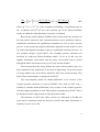
The theoretical improvements have been made in the unified HauserFeshbach and exciton model. The angular momentum conservation is considered
in whole reaction processes for both equilibrium and pre-equilibrium mechanism.
The recoil effects in varied emission processes are taken into account strictly, so
the energy balance can be held exactly. A method for calculating doubledifferential cross sections of composite particles is proposed. Based on this
theoretical frame, the UNF code (2001 version) for calculating neutron induced
reaction data of structure materials below 20 MeV was issued. The functions of
the UNF code are introduced.
Introduction
For fast neutron reaction data calculations, there are several widely used
computer code, such as GNASH (Refs.[1] and [2]) and TNG (Ref.[3]), which are
useful for fast neutron evaluation. The equilibrium and the pre-equilibrium
statistical mechanism are employed in both codes, but in different approach. In
the theoretical description of the model there are still some thing could be
improved. The first point is about the emissions of the first outgoing particles,
there should be three types of emission mechanisms, i.e. direct emission, preequilibrium emission and equilibrium emission. In particular, the emission from
compound nucleus to the discrete levels of the residual nuclei, each of which has
31
its individual spin and parity. Therefore the angular momentary conservation and
parity conservation should be taken into account properly. These three types of
emission mechanisms have been taken into account in both GNASH code and
TNG code. But GNASH code does consider the angular momentum conservation
in the pre-equilibrium part of the calculations. The TNG code is based on a
unified model, in which the lifetime of particle-hole states are independent of
spin, which imply that the angular momentum conservation in the preequilibrium process is not included. So locating a proper approach to describe
the pre-equilibrium emissions from compound nucleus to the discrete levels is
required, which needs to develop an angular momentum dependent exciton
model. It is introduced in Sec.B1. Combining with the Hauser-Feshbach model,
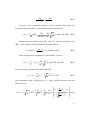
this kind of reaction mechanism can be described based on the unified HauserFeshbach and exciton model[4]. In this model the formula of the energy spectrum
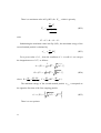
reads as follows:
W Jπ (n, E*, ε )
dσ
= ∑ σ aJπ ∑ P Jπ (n) b Jπ
Jπ
n
dε
WT (n, E*)
(B1)
where σ aJπ stands for the absorption cross section, P Jπ (n) refers to the
occupation probability of the n exciton state in the jπ channel, which can be
obtained by solving the j-dependent exciton master equation to conserve the
angular momentum in the pre-equilibrium reaction processes, WbJπ ( n, E*, ε ) is
the emission rates of particle b at exciton state n with outgoing energy ε .
Obviously, if we do not consider the parity and angular momentum effects,
Eq.(B1) is reduced to the exciton model, while if the pre-equilibrium effect is
omitted, Eq.B1 is reduced to the Hauser-Feshbach model. In the case of low
incident energies (En ≤ 20 MeV), only n=3 is taken into account for the preequilibrium mechanism. Therefore, the formula of the energy spectrum in
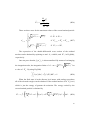
practical calculation reads
32

W jπ (3, E*, ε )
W jπ ( E*, ε ) 
dσ
= ∑ σ ajπ  P jπ (3) b jπ
+ Q jπ (3) b jπ

jπ
dε
WT (3, E*)
WT ( E*) 

(B2)
where Q jπ (3) = 1 − P jπ (3) is the occupation probability of equilibrium state in
the jπ channel and WbJπ ( E*, ε ) is the emission rate in the Hauser-Feshbach
model, in which the width fluctuation correction is included.
Based on the unified Hauser-Feshbach and exciton model the emissions of
the first particle emissions from compound nucleus can be described with preequilibrium mechanism and equilibrium mechanism as well as direct reaction
process. In this model the angular momentum depended exciton model is used
for conserving angular momentum in the pre-equilibrium emission processes. At
low incident energies (En≤20 MeV), the secondary particle emissions are
described by multi-step Hauser-Feshbach model. To do so in this way the
angular momentum conservation and the parity conservation can be carried
through the whole reaction processes up to (n,3n) reaction channel.
The second point is the energy balance for each reaction channel, since it is
quite important in the application of the nuclear engineering. To meet the needs
of energy balance the recoil effects should be taken into account strictly. This
kind of accurate kinematics is introduced in Sec B2.
The semi-empirical model for double-differential cross sections of the
complex particles emissions is used in GNASH code, while in UNF code, a
method to calculate double-differential cross sections of the complex particles
with the pickup mechanism is used. This method is introduced in Sec.B3. This is
the third point on the improvements of the theoretical model.
The functions of UNF code (2001 version) are elaborated in Sec.B4 and
some typical calculated results are shown in Sec.B5 with some discussions. A
summary is given in Sec. B6.
33
B1
Angular Momentum Coupling Effect in Pre-Equilibrium
Particle Emission
To consider the angular momentum and parity conservation the angular
momentum (J) and parity ( π ) should be addressed in the master equation of
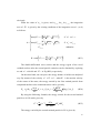
exciton model, so the master equation of jπ channel reads
dq Jπ (n, t )
= λ J+π (n − 2)q Jπ (n − 2, t ) + λ J−π (n + 2)q Jπ (n + 2, t )
dt
- [λ J+π ( n) + λ J−π ( n) + Wt Jπ ( n)]q Jπ ( n, t )
(B3)
where λ J±π is the internal transition rate and Wt Jπ is the total emission rate of the
exciton state in jπ channel. The jπ dependent internal transition rate can be
written in the form
λ Jvπ = λ v ( n) χ J (n),
v = +,0,−
(B4)
Where λ v ( n) is the internal transition used in the usual jπ independent exciton
model, while χ J (n) stands for the angular momentum factor. In FKK model[5]
the angular momentum conservation was considered properly. Following the
approach of FKK model the angular momentum factor can be constructed. But in
FKK model only spin-zero nucleon was used. In this paper the spin-1/2 nucleon
is used to provide the angular momentum factor.
The δ type residual two-body interaction is used for the particle-hole
excitation, which can be expanded in the form as follows:
δ( r1 − r2 ) =
δ(r1 − r2 )
*
YKm
(rˆ1 )YKm (rˆ2 )
∑
Km
r1 r2
Applying the basic formula, the reduced matrix elements are defined by
34
(B5)
j ' m'
j ' m' TLM jm = C LM
jm j ' ' TL j
(B6)
J ' m'
j ' TL j = ∑ C LM
jm j ' m ' TLM jm
(B7)
and:
Mm
Where C is the Clebsch-Gordon coefficient. The tenser product of T p and T q
satisfies the equation as
mr
[T pU q ]rmr = ∑ C pmr p qm
Tmpp Tmqq
g
(B8)
Thus the reduced matrix element is obtained by
ja , jb , j [T p ⋅ U q ]r jc , jd , j ' =
∑C
mr m '
ja j b , jm [T p × U q ]rm jc jd , j ' m'
j m
rmr j ' m '
r
r m
C pmj mj m C qmj mj m ja Tmp jc
= ∑ C rmj mj 'm ' C jj mmj m C jj 'm mj 'm C pm
qm
a
r
r
= ( −1)
j + j ' + p +q+r
a
a b
b
c
c d
d
p
a
p c
g
b
c
b
q d
d
p
 ja j b j 
ˆ'
j


ˆj ˆj
(2 j + 1) jc jd j ' ja T p jc
a b
rˆ
p q r 


where ˆj ≡ 2 j + 1 and
j b U mq jd
q
j b U q jd
(B9)
{ } is the 9-j coefficient.
Using
T p ⋅ U p = ( −1) p pˆ [T p × U p ]0
0
and
 ja j b j 
j + p− j − j

 (−1)
'
j
j
j
=
W ( ja jc jb jd , p j )δ jj '
 c d 
ˆjpˆ
p p 0 


a
d
(B10)
we have
ja j b j T p ⋅ U p jc jd j ' = ˆja ˆj b ˆjˆj ' (−1) j− j − j δ jj 'W ( ja jc j b jd , j p )
a
d
35
j a T p jc
j b U p jd
(B11)
In our case, T p = Y p and U p = Y p , where Yp stands for the spherical
harmonics function. The derivation procedure can be found in Ref.[6] in detail.
For the nucleon with spin=1/2, the antisymmetrization needs to be taken into
account.
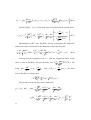
In the case of λ + , a particle ( ja ) creates a particle-hole ( j b , jd ) . Besides
the particle a and the particle-hole b and d, the residual part of the compound
nucleus is called observer, which has the spin S. The angular momentum
coupling triangle relations ∆( J , ja , S ), ∆ ( jb , jd , j3 ) , ∆ ( j3 , jc , ja ) must be held
to keep the angular momentum conservation in the pre-equilibrium process. The
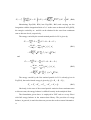
final result of the angular momentum factor of χ +J is obtained by
χ +J (n) =
1
∑ Rn −1 ( s) R1 ( ja )F+ ( ja )∆( ja JS )
32π Rn ( J ) sj
2
(B12)
a
F+ ( ja ) = ∑
j3 j c
1
(2 jc + 1) R1 ( jc )G+ ( ja jc j3 )
2 j3 + 1
(B13)
G+ ( ja jc j3 ) = ∑ (2 j b + 1)(2 jd + 1)R1 ( j b ) R1 ( jd )
jb jd
[C j 1 0 1 C j 1 0
3
ja
3
2
jc −
2
jb
2
jd −
+ (−1) j + j C j 1 0 1 C j 1 0 1 ]2
c
1
2
d
3
ja
3
2
jd −
2
jb
2
jc −
(B14)
2
For the case of χ −J ，a particle ( ja ) annihilates a particle-hole pair ( j b jd , j3 ) ,
the derivation procedure is as the same as that of χ +J . In this case only the weight
Rn−3 ( s ) is used instead of Rn−1 ( s ) in Eq.(B12).
Being consistent with the independent exciton model, the angular
momentum factors satisfy the normalization condition
36
∑ (2 J + 1) R ( J ) χ = 1, v = +,0 −
n
J
J
v
(B15)
where Rn (J ) is the spin distribution factor of angular momentum in n exciton
state
Rn ( J ) =
2J + 1
2π 2σ n3
1
− (J + )2
2 ]
exp[
2
2σ n
(B16)
2
where σ n = 0.24nA 3 refers to the spin cut-off factor of the n exciton state
for the nucleus with the mass number A, σ n is independent of energy.
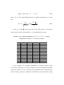
Table B1 The occupation probabilities of Q
absorption cross section
σ ajπ
jπ
(n = 3) , P jπ (n = 3) and the
of 54Fe at En=12 MeV
j
Q jπ (3)
P jπ (3)
σ aj + (b)
σ aj − (b)
0.5
0.4371
0.5629
3.586E-02
3.871E-02
1.5
0.5928
0.4072
7.173E-02
7.412E-02
2.5
0.6722
0.3278
1.263E-01
1.112E-01
3.5
0.7236
0.2764
1.684E-01
1.191E-01
4.5
5.5
0.7620
0.7929
0.2380
0.2071
1.711E-01
2.053E-01
1.489E-01
4.345E-02
6.5
0.8175
0.1825
5.649E-03
5.070E-02
7.5
0.8372
0.1628
6.456E-03
7.689E-04
8.5
0.8519
0.1481
1.032E-04
8.651E-04
9.5
0.8623
0.1377
1.146E-04
1.347E-05
10.5
0.8676
0.1324
1.721E-06
1.482E-05
11.5
0.8681
0.1319
1.877E-06
2.160E-07
12.5
0.8611
0.1389
0.000E+00
2.340E-07
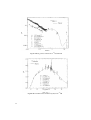
As an example, the occupation probabilities at incident neutron energy
En=12 MeV for different j are given in Table B1 to show the angular momentum
conservation effect. For low j region the pre-equilibrium state is dominant part,
while for high j region the equilibrium contributions become important, which
37
means that the components with high j in compound nucleus need multi-step
intrinsic-collision processes. Averaged by the absorption cross section, the preequilibrium emission occupies the percentage of 28.86%, while the equilibrium
emission occupies 71.14 %.
B2 Recoil Effect and Energy Balance
The energy balance for whole reaction processes must be taken into account
to set up neutron data file for application. For each reaction channel with a
reaction Q value, the released total energy includes the energies of the outgoing
particles E p , the recoil nucleus E R , and the gamma decay energy Eγ . The
energy balance needs
E R + E p + Eγ = E n + Q
(B17)
where En stands for the incident neutron energy in laboratory system (LS). If the
recoil nucleus is assumed static in the center of mass system (CMS) after
sequential particle emission, in this way neither the accurate shape of outgoing
particle spectra nor the energy balance could be obtained. This paper will give
the formulation of the energy balance of the secondary particle emissions, which
is employed in the UNF code. In UNF code only the sequential particle
emissions are taken into account.
The particle emissions have three cases, (1) from continuum states to
continuum states, (2) from continuum states to discrete levels, (3) from discrete
levels to discrete levels, of which the formulation has been given in Ref. [7].
Beside the laboratory system (LS) and the center of mass system (CMS),
the recoil nucleus system (RNS) is also needed, which is a moving system along
with the recoil residual nucleus. The physical quantities are labeled by subscripts
l,c,r, respectively for the three motion systems. At low incident energies (<20
38
MeV), the pre-equilibrium mechanism is taken into account only for the first
particle emissions, while the isotropic distribution is employed for the second
emission particles in RNS. In this case the double-differential cross sections of
the secondary particle emissions in CMS can be easily obtained.
The physical quantities used in this paper are defined as following :
E*=
MT
E n + Bn : excitation energy;
MC
Bn: binding energy of incident neutron in compound nucleus;
MT, MC : masses of target and compound nucleus, respectively ;
m1, m2: mass of the first and the second emitted particle, respectively;
ε1, ε2: energy of the first and the second emitted particle, respectively;
M1, M2: mass of residual nucleus after the first and the second emitted
particle, respectively;
E1,E2: energies of residual nuclei after the first and the second particle
emissions, respectively,
B1, B2: binding energy of the first and the second emitted particle in its
compound nucleus, respectively;
Ek1 , Ek 2 : level energy with the level order number k1, k2 reached by the first
and the second emitted particle, respectively;
f l (ε mc ) : Legendre expansion coefficient of the first emitted particle in
1
CMS.;
f l (ε mc ) : Legendre expansion coefficient of the second emitted particle in
2
CMS;
B2.1
Double Differential Cross Section from Continuum State to
Continuum State
Based on the relation of the double differential cross sections between CMS
39
and RNS
d 2σ
d 2σ
c
c
d
d
dΩ r dε r
=
Ω
ε
c
c
r
r
dΩ dε
dΩ dε
(B18)
The Jacobian is given by
εc c
dε ′ d Ω =
dε d Ω c
r
ε
r
r
(B19)
The normalized double differential cross section in the standard form reads
d 2σ
2l + 1
=∑
f l (ε )Pl (cosθ )
l
dεdΩ
4π
(B20)
where Pl (cosθ) refers to the Legendre polynomial. Averaged by the doubledifferential cross section of the residual nucleus after the first particle emission,
the double-differential cross section of the second particle emission can be
obtained by
d 2σ
d 2σ
d 2σ
=∫
dε mc dΩ mc
dE Mc dΩ Mc dε mr dΩ mr
2
2
1
≡∑
l
1
2
ε mc
2
εm
r
2
dE Mc dΩ Mc
1
1
(B21)
1
2l + 1
f l (ε mc )Pl (cosθ mc )
4π
2
2
where the double-differential cross section of the residual nucleus of M 1 has the
form
d 2σ
2l + 1
f l ( E Mc )Pl (cosθ Mc )
=∑
c
c
l
dE M dΩ M
4π
1
1
1
(B22)
1
The isotropic distribution of the second particle emission in RNS reads
40
d 2σ
1 dσ
=
r
r
dε m dΩ m
4π dε mr
2
2
(B23)
2
In terms of the orthogonal property of the Legendre polynomial, the
Legendre coefficient of the second emitted particle is obtained by
1
d 2σ
dσ
c
f l (ε m ) =
dΩ m
∫
4π
dE Mc dΩ Mc dε mr
ε mc
c
2
ε
2
1
1
2
2
r
m2
Pl (cosθ mc )dE Mc dΩ Mc (B24)
2
1
1
Denoting Θ as the angle between Ω Mc and Ω mc , then the integration over
1
2
dΩ m can be replaced by dcosΘ dΦ, and using the relation
c
2
PL (cosθ mc ) =
2
4π
∑m YLm* (Θ ,Φ )YLm (Ω Mc )
2L + 1
Then carrying out the integration over dcosΘ dΦ
1
dσ
f l (ε m ) = ∫ f l ( E Mc ) r
2
dε m
ε mc
c
2
(B25)
1
1
2
ε
2
r
m2
we have
Pl (cosΘ )dE Mc d cosΘ
(B26)
1
From the energy relation between RNS and CMS
ε mr = ε mc +
2
2
m2 c
m2 c c
EM − 2
E M ε m cosΘ
M1
M1
1
1
(B27)
2
and substituting cosΘ in Eq.(B26) by ε mr , then Eq.(B26) becomes into the
2
following form
f l ( E Mc ) b dε mc
1 M1 B
c
f l (ε m ) =
∫ dE M
∫
4 m2 A
E Mc a ε mr
c
1
2
2
2
1
1
 c
 ε m + m2 E Mc − ε mr
M1
dσ 
Pl 
r
dε m 
m2 c c
 2 M EM ε m
1

2
1
2
1
2
2



 (B28)



41
For the given values of ε mc
and E Mc , by means of the condition
2
1
− 1 ≤ x ≤ 1 for the Legendre polynomial of Pl ( x ) , the integration limits of a and
b in Eq.(B28) are given by
2

 c
m2 c  
r
a = max ε m ,min ,  ε m −
E M  
M
1


 
2




m
2
b = min ε mr ,max ,  ε mc +
E Mc  
M1


 
2
2
2
1
2
(B29)
1
In terms of the velocity composition relation of v mr and v Mc , the energy
2
1
region of the second particle emission is obtained by
ε m , max
c
2
εm
c
2
, min

 ε mr



=  ε mr





2
2
, max
, min
 m2 c
E M , max + ε mr , max
= 
 M1
1
−
m2 c
EM
M1
−
m2 c
EM
M1
1
1
2
, min




2
, max








2
if ε mr
if
0
2
, max
1
(B30)
m2 c
EM
M1
<
m2 c
EM
M1
2
, max
< ε mr
1
, min
(B31)
2
, min
othewise
When f 0 ( E Mc ) is normalized, the f 0 (ε mc ) is also normalized. By means of
1
2
exchanging the integration order, the integration limits of
( ε mr ±
2
ε mc
2
are
m2 c 2
E M ) for every values of ε mr and E Mc . By using Eq.(B28)
M1
2
1
ε mc 2 , max
1
dσ
∫ f (ε )dε = ∫ f ( E )dE ∫ dε dε = 1
0
ε mc 2 , min
c
m2
c
m2
0
c
M1
c
M1
r
r
m2
(B32)
m2
It is easy to see from Eq.(B30) that the scope of the outgoing energy
spectrum is broadened, when the recoil effect is taken into account. The lighter
of the nucleus, the stronger of recoil effect and the broad effect even more
42
obviously.
When the value of ε mc is given, and ε mc ,min ≤ ε mc ≤ ε mc ,max the integration
2
2
2
2
area of E M is given by the existing condition of the integration over ε mr (a<b)
c
1
2
as follows:
M1

c
max{
,
E
M
,
min

m2

M

A = max{EMc ,min , 1
m2


EMc ,min


1
1
(ε
(ε
c
m2
)
if ε mc > ε mr ,max
)
if ε mc < ε mr ,min
2
− ε mr ,max }
2
2
2
r
m 2 . min
− ε mc }
2
2
2
2
othewise
1

M
B = min  E Mc , max , 1
m2

1
(ε
c
m2
)

+ ε mr , max 

2
(B33)
The double-differential cross section and the energy region of the recoil
residual nucleus after the second particle emission can be obtained by replacing
m2 and ε mr with M2 and E Mr in Eq.(B28), respectively.
2
2
On the other hand, one can prove the energy balance is held in an analytical
way. By means of the velocity v ml = VC + v mc , where VC is the motion velocity
1
1
of the center of the mass; the energy carried by the first emitted particle from
compound nucleus to the continuum states can be given by
Eml = ∫ dε mc {(
1
1
2 mn m1
mn m1
En + ε mc ) f 0 (ε mc ) +
2
MC
MC
1
1
En ε mc f1 (ε mc )}
1
1
(B34)
By using the following formula, the energy carried for the second emitted
particle m in LS can be given by
d 2σ
m
l 2
E = ∫ (v )
dE Mc dΩ Mc
c
c
2
dE M dΩ M
l
1
1
1
(B35)
1
The energy carried by the second emitted particle in LS is given by
43

mn m2
c  mn m2
c
c
c
d
ε
∫ m  M 2 En f 0 (ε m ) + ε m f 0 (ε m ) + 2 M
 C
C
Eml =
2
2
2
2

En ε mc f1 (ε mc ) (B36)

2
2
2
From Eq.(B28), f 1 (ε mc ) in the third term in Eq.(B36) has the explicit form
2
f1 ( EMc ) b dε mr
1 M1 B
c
f l =1 (ε m ) =
∫ dE M
∫
4 m2 A
ε mr
EMc a
c
1
2
2
2
1
1
 c
 εm +
dσ 
dε mr 
 2


2
1
m2 c
EM − ε mr
M1
m2 c c
EM ε m
M1
1
2
1
2



 (B37)



Substituting Eq.(B37) into Eq.(B36), and by exchanging the integration
order as the same as in Eq.(B32), the third term in Eq.(B36) becomes
f1 ( E Mc ) dσ dε mr
mn E n
c
∫ dE M E c ∫ dε r
m2
ε mr
M
m
1 M1
4 MC
1
1
2
m2
∫ dε {ε + M E − ε }
2
1
c
c
m2
m2
c
r
M1
m2
(B38)
1
2
Carrying out the integration over ε mc with the integration limits as the
2
m2
M1
m2 M m M
Ec ε r Ec . By
M1
, and f 1 ( E Mc ) = −
M1
f 1 (ε mc ) , the third
m1
same as that in Eq.(B32), this part becomes into 8
dσ
m1
∫ dε dε = 1 , E = M ε
r
using
m2
c
M1
r
c
m1
1
1
m2
1
2
1
1
term in Eq.(B36) is reduced into
mn m1 m2
dε mc
∫
M C M1
−2
1
En ε mc f1 (ε mc )
1
1
The second term in Eq.(B36) can be reduced by
∫ ε f (ε )dε
c
m2
0
c
c
m2
m2
c
1 M 1 f 0 (EM ) c
dE M
= ∫ dε m
∫
4 m2
E Mc
c
1
2
1
∫
1
dε mr dσ c
εm
r
ε mr dε m
2
2
2
2
c
r
1 M 1 f 0 ( E M ) dε m dσ 1 c 2 (
= ∫ dE M
∫ r dε r 2 (ε m ) |(
4 m2
E Mc
εm
m
c
1
2
1
2
1
44
2
2
m2 c
EM + ε mr 2 ) 2
M1 1
m2 c
EM − ε mr 2 )2
M1 1
= ∫ dE Mc f 0 ( E Mc ) ∫ dε mr
1
1
2
dσ m 2 c
E M + ε mr )
(
r
dε m M 1
1
2
2
=
m1 m2
dσ r
dε mc f 0 (ε mc )ε mc + ∫ dε mr
εm
2 ∫
dε mr
M1
2
2
2
2
(B39)
2
2
Thus, the energies carried by the second emitted particle is obtained by
Eml =
2
mm
dσ r
mn m2
εm
En + 1 2 2 ∫ dε mc f 0 (ε mc )ε mc + ∫ dε mr
2
M1
dε mr
MC
2
2
2
2
2
2
(B40)
mn m1 m2
En ∫ dε mc f1 (ε mc ) ε mc
−2
M C M1
1
1
1
In terms of the same procedure for m2 the energy carried by its residual
nucleus M 2 can be obtained by
mn M 2
mM
m
dσ r
En + 1 2 2 ∫ dε mc f 0 (ε mc )ε mc + 2 ∫ dε mr
εm
2
MC
M1
M2
dε mr
E Ml =
2
2
2
2
2
2
2
mn m1 M 2
−2
M C M1
(B41)
En ∫ dε m f1 (ε m ) ε m
c
c
1
c
1
1
The γ de-excitement energy is obtained by the averaged residual excitation
energy
d 2σ
d 2σ
[
E * − B1 − B2 − ε mc − ε mc − EMc ]dε mc dε mc dΩ mc dΩ mc
c
c
c
c
dε m dΩ m dε m dΩ m
(B42)
= E * − B1 − B2 − ∫ ε mc f0 (ε mc )dε mc − ∫ ε mc f0 (ε mc )dε mc − ∫ f0 ( EMc ) EMc dEMc
Eγl = ∫
1
2
2
1
2
1
1
2
1
2
1
1
1
1
2
2
2
1
1
1
where
m1 m2
dσ
∫ ε f (ε )dε = M ∫ dε f (ε )ε + ∫ dε dε ε
c
m2
0
c
c
m2
m2
c
m1
2
0
c
c
r
m1
m1
m2
r
c
M2
0
c
c
M2
M2
(B43)
m2
1
m1 M 2
∫ E f ( E )dE = M
r
m2
2
1
m2
dσ
∫ dε f (ε )ε + M ∫ dε dε ε
c
m1
0
c
m1
c
m1
2
r
m2
r
r
m2
(B44)
m2
Therefore,
45
Eγl = E * − B1 − B2 −
MC
M
dσ r
dε mc f 0 (ε mc )ε mc − 1 ∫ dε mr
εm
∫
M1
M2
dε mr
1
1
1
2
2
(B45)
2
It is easy to see that if the recoil effect is not taken into account, the residual
nucleus is static in CMS, in this way the energy carried by the second emitted
particle only has the second term in Eq.(B43), while the first term is the energy
gain by recoil effect. From Eq.(B43) one can see that the recoil effect increases
with the decreasing of the mass of residual nucleus, and with the increasing of
the mass of emitted particles.
The total released energy can be obtained by summing over Eqs.(B36, B40,
B41 and B45)
ETl = Eml + Eml + EMl + Eγl = En + Q
1
2
2
(B46)
Here, Q = Bb − B1 − B2 is the reaction Q-value in the two particle
emission process. Therefore, the energy balance is held exactly in the analytical
form.
From the afore-mentioned formulation, one can see that the quantity of the
Legendre expansion coefficient with l=1 ( f 1 (ε mc ) >0) plays an important role in
1
the energies carried by different kinds of emitted particles, which is caused by
the forward emission of the first emitted particle in the pre-equilibrium process.
If f 1 (ε mc ) increases, then the energy carried by the first emitted particle
1
increasing in LS, while the recoil effect reduces the energies of the second
particles emitted from the recoil residual nuclei due to the motion of the center of
mass system. Meanwhile, the shape of f 0 (ε mc ) can also influence the energy
1
distributions between the emitted particles, the residual nucleus and de-excitation
γ energy. The harder of the spectrum, the more energy carried by the emitted
particle, while the energies carried by the residual nucleus and de-excitation γ
emissions are reduced. But in pure equilibrium emission process, either isotropic
approximation or the Hauser-Feshbach theory，the partial wave with l=1 of the
Legendre expansion is zero, only the energy distributions for all of kinds of the
46
emitted particles are influenced by the shapes of the first emitted particle.
B2.2 Double Differential Cross Sections from Continuum State to Discrete
Levels
When the residual nucleus is in discrete level states, the double differential
cross section has different expression since ε mr is a single value. In this case
2
dσ
1
= δ(ε mr − ε mr ,k )
r
r
dε m dΩ m
4
2
2
2
(B47)
2
2
where ε mr is the function of E Mc and has the value as
1
2 ,k
M
M2
( E * − B1 − B2 − Ek − C E Mc )
M1
m1
ε mr ,k ( EMc ) =
2
1
2
(B48)
1
The Legendre coefficient in Eq.(B38) becomes into the form
1 M1 B
f l (ε m ) k =
∫
4 m2 A
c
2
f l ( E Mc )
Pl (cosΘ )dE Mc
1
ε m ,k E M
r
c
2
1
(B49)
1
with
m2 c
E M + ε mc − ε mr , k
M
cosΘ = 1
m2 c c
2
EM ε m
M1
1
2
2
1
(B50)
2
For a value of E Mc the maximum energy of the second emitted particle
1
ε m , max should correspond to the direction of the second emitted particle with the
c
2
same direction of the first outgoing particle.
 m2 c
E M + ε mr , k
ε m , max ( E M ) = 
 M1
c
c
2
1
1
2




2
(B51)
47
There is a maximum value in Eq.(B51) for E Mc , which is given by
1
Eˆ Mc
1
m1
E k′
MC
=
M M
1+ C 2
m1 m2
(B52)
with
E k′ = E * − B1 − B2 − E k 2
Substituting the maximum value into Eq. (B51), the maximum energy of the
second emitted particle is obtained by
ε mc
2 , max
=
m1
RE k'
MC
(B53)
For a given value of ε mc , from the condition of -1 ≤ cosΘ ≤ 1 one can get
2
the integration area of E M as follows
c
1
A = {E Mc ,min ,
1
B = {E Mc , max ,
1
where R =
m2 c 2
1
( U−
εm ) }
2
R
M1
2
m2 c 2
1
( U+
εm ) }
2
R
M1
(B54)
2
M
m2 M 2 M C
M
; U = 2 ( REk′ − C ε mc ) .
+
M 1 M 1 m1
M1
m1
2
The minimum energy of the second emitted particle ε cm, max corresponds to
2
the opposite direction of the first outgoing particle.
 m2 c
E M − ε mr , k
ε m ，, min ( E M ) = 
 M1
c
c
2
There is a zero point at
48
1
1
2




2
(B55)
(
E Mc
1
M2
E k′
m2
=
M M
1+ C 2
m1 m2
(B56)
There are three cases for the maximum values of the second emitted particle
 m2 c
E M , min － ε mr , k ) 2
(
 M1

= 0

( ε r − m2 E c
)2
m ,k
M , max

M1

1
ε mc , min
2
(
if E Mc ≤ E Mc , min
2
2
1
1
(
if E Mc , min < E Mc < E Mc , max (B57)
1
1
(
if E Mc , max ≤ E Mc
1
1
1
1
The expression of the double-differential cross section of the residual
nucleus can be obtained by replacing m2 and ε mr with M2, and E Mr in Eq.(B49),
2
2
respectively.
One can prove that the f 0 (ε mc ) k is also normalized. By means of exchanging
2
the integration order, the integration limits of ε mc are ( ε mr , k ±
2
2
m2 c 2
E M ) for
M1
1
a value of E Mc . By using Eq.(B49)
1
ε mc 2 , max
∫ f (ε )dε = ∫ f ( E )dE = 1
0
ε mc 2 , min
c
c
m2
m2
0
c
c
M1
M1
(B58)
When the final state is in the discrete level states, with analogy procedure
all of the released energies can be obtained. If the residual nucleus is in E k level,
2
which is just the energy of gamma de-excitation. The energy carried by the
second emitted particle is obtained by
 m m
Eml ,k = ∫  n 2 2 En + ε mc
 M C
2
2
mn m2

 f 0 (ε mc ) k +2
MC

2

En ε mc f1 (ε mc ) k dε mc

2
2
2
(B59)
49

En EMc f1 ( E Mc ) k dEMc (B60)

Substituting Eqs.(B49, B50) into Eqs.(B59, B60) and carrying out the
 m M
EMl ,k = ∫  n 2 2 En + E Mc
 M C
1
1
mn M 2

 f 0 ( E Mc ) k +2
MC

1
1
1
1
integration with the integration limits of ε mc as the same as that used in Eq.(B58),
2
the energies carried by m2 and M2 can be obtained in the case from continuum
state to discrete levels, respectively.
The energy carried by the second emitted particle in LS is given by
Eml ,k =
2
mn m2
M
En + 2 ( E * − B1 − B2 − Ek )
2
MC
M1
2
−(
−2
M C M 2 m1 m2
) ∫ dε mc f 0 (ε mc )ε mc
−
M 12
M 12
1
mn m1
MC
En
m2
M1
1
(B61)
1
∫ f (ε ) ε dε
1
c
c
c
m1
m1
m1
and
EMl
2 ,k
=
mn M 2
m
En + 2 ( E * − B1 − B2 − Ek )
2
M1
MC
2
−(
−2
M C m2 m1 M 2
) ∫ dε mc f 0 (ε mc )ε mc
−
2
2
M1
M1
1
mn m1
MC
En
M2
M1
1
∫ f (ε ) ε dε
1
(B62)
1
m1
c
c
c
m1
m1
The energy carried by the first emitted particle in LS is already given in
Eq.(B34), the total released energy is given by ( Q = Bn − B1 − B2 ),
ETl ,k = Eml + Eml ,k + EMl
1
2
2 ,k
+ Eγl ,k = En + Q
(B63)
Obviously, in the case of the second particle emission from continuum state
to discrete state, the energy balance is still held exactly in the analytical form.
The formulation given above is employed in UNF code to set up files-6
with full energy balance in the neutron data library. The precision of energy
balance, in general, is much less than one percent due to the accurate kinematics.
50
B3
Double-Differential Cross Section of Composite Particle
Emissions
The pickup mechanism should be involved in the composite particle
emission to give the pre-formation probability of composite particle in
compound nucleus. At first the Iwamoto- Harada model[8] has been employed in
UNF code. But the calculated result indicated that this model overestimated the
pre-formation probabilities of the composite particles. The study turns out that
the integration over momentum space in the phase space integration has the
superfluous part, which is the forbidden area restricted by excitation energy. So
the E-dependent improved Iwamoto- Harada pickup mechanism was developed[9]
to reduce the pre-formation probabilities, and used in UNF code.
The double-differential cross sections of single nucleon can be calculated by
generalized master equation[10,
11]
to get the angular momentum dependent
lifetime τ (n, Ω) with the Legendre expansion form as
τ (n, Ω ) = ∑ ζ l (n)Pl (cos θ )
(B64)
l
The double-differential cross section of particle b is represented by
d 2σ
dσ (n)
A(n, ε b , Ω b )
=∑
dΩ b dε b n dε b
where
(B65)
dσ (n)
= component of n exciton state in the spectrum.
dε b
In the case of composite particle emission, the outgoing nucleon may pickup
some nucleons below and above the Fermi surface to form a composite particle
to be emitted. According to the studies on pickup mechanism, at low energies
(En≤20 MeV), the dominant configuration is pickup the nucleons below the
Fermi surface[12].
The angular distribution factor in Eq.(B65) of b particle with emitted energy
51
ε b and direction Ω b at n exciton state is introduced by
A(n, ε b , Ω b ) =
A
A
1
d
p
,
L
,
d
p
(
p
p
)
D(V j )τ (n, Ω 1 ) (B66)
δ
−
∑
∏
∫ 1
A
i
b
i =1
j =2
N
b
b
b
with p1 > pf and p j < pf for j=2,…,Ab.
where τ ( n, Ω 1 ) = lifetime of the outgoing single nucleon marked by 1
pf = Fermi momentum
pb = momentum of outgoing composite particle b with mass number Ab.
D = momentum distribution of the compound nucleus
N = normalization factor.
The δ function in Eq.(B66) implies momentum conservation. Obviously, if
emitted particle b is a nucleon, then Eq.(B66) will return to the case of single
nucleon emission. The Fermi gas model is employed to give the momentum
distribution of the nucleon below the Fermi surface.
D ( p ) dp =
3
Θ ( pf − p)dp
4πpf3
(B67)
The procedure to carry out the integration analytically over the angle and the
momentum of Eq.(B66) can be found in Refs.[13] and [14], which is reduced
into the following form
Ab (n, ε b , Ω ) =
ζ ( n)
1
∑l l Rb (ε b )Pl (cos θ b )
4π ζ 0 ( n)
(B68)
The factor Rb (ε b ) in Eq.(B68) is defined by
Rl (ε b ) =
Gl (ε b )
G0 (ε b )
(B69)
where
1+ E / ε f
Gl (ε b ) =
∫ dx1 x1
max{1, xb − Ab +1}
E = excitation energy
52
Ab −1
∫
xb − x1
Z b ( y )Pl (
xb2 + x12 − y 2
) ydy
2 xb x1
(B70)
ε f = Fermi energy
x1 =
p1
= dimensionless momentum of particle 1
pf
xb =
pb
= dimensionless momentum of particle b
pf
y = xb2 + xc2 − 2 xb x1 cos θ
The final result of Z b ( y ) in Eq.(B70) is obtained as follows:

1
b=d

 1
b = t ,3 He (B71)
Z b ( y ) = (1 - y ) 2 (4 + y )
2

 (3 - y) 4
2
3
 y [210 − 120(3 − y ) + 21(3 − y ) − (3 − y ) ] b = α

In Eq.(B68), the partial wave coefficients ζ l (ε ) of
single nucleon
emission are calculated by the linear momentum dependent exciton state density
model[15]. This approach is a consistent way to obtain the angular distribution of
outgoing nucleons. In this method the leading particle is not assumed; instead, a
statistical population of all states compatible with energy and momentum
conservation is proposed. The effects of the Fermi motion of the nucleons, as
well as the Pauli blocking by the “sea” of nucleons, are included. In particular,
the angular distribution from the first pre-equilibrium state in a nucleon-induced
reaction is identical to that obtained with the Kicuchi-Kawai scattering
kernel[16,11].
There is no any additional free parameter in this method, which should be
pointed out emphatically.
53
B4 Functions of UNF Code
The UNF code (2001 version) was developed for calculating fast neutron
reaction data of structural materials with incident energies from a few kiloelectron-volts to 20 MeV. This code can handle a decay sequence up to (n,3n)
reaction channel, including 14 reaction channels. The physical quantities
calculated by UNF code contain the follows:
(1) Cross sections of total, elastic scattering, non-elastic scattering, and all
reaction channels in which the discrete level emissions and continuum
emissions are included.
(2) Angular distributions of elastic scattering both in CMS and LS.
(3) The energy spectra of the particle emitted in all reaction channels.
(4) Double-differential cross sections of all kinds of particle emissions
(neutron, proton, alpha particle, deuteron, triton and 3He), as well as the
recoil nuclei.
(5) Partial kerma factors of every reaction channels, and the total kerma
factor.
(6) Gamma production data (gamma spectra, gamma production cross
sections, and multiplicity), including the gamma production cross
sections from level to level.
(7) Total double-differential cross sections of all kinds outgoing particles
from all reaction channels.
(8) Cross sections of isomeric states, if the level is a isomeric state of the
residual nucleus.
(9) dpa cross sections used in radiation damage.
UNF code can also handle the calculations for a single element or for
natural nucleus, and the target can be in ground state or in isomeric state.
Besides the output file, the outputting in ENDF/B-6 format is also included,
(files3, 4, 6, 12, 13, 14, 15 or files-3, 4, 5, which controlled by a flag).
54
Meanwhile, some self-checking functions are designed for checking the
errors in the input parameter data, if it exist.
B5 Calculated Examples and Discussion
Some calculated results have been shown in Ref.[4]. A large number of
figures to compare the calculated results with the measured data have been
published in “Communication of Nuclear Data Progress” INDC(CRP)-041/L to
053/L as technical reports during the evaluations of the nuclei for CENDL-3.
Some typical calculated examples are given below.
The capture radiation cross section of n+160Gd is shown in Fig.B1. In UNF
code the gamma de-excitation has three mechanisms; (1) equilibrium gamma
emission, (2) pre-equilibrium gamma emission, (3) direct gamma emission. The
Oblozinsky’s formula[17] is employed for the last two terms. A small peak occurs
at about 14 MeV in the capture radiation cross section, which is the contribution
from the direct gamma emission.
The (n,2n) reaction cross section of n+150Nd is shown in Fig.B2. The
calculated results agree fairly well with the experimental measurements.
All of the measured data used in Fig.B1 and Fig.B2 are retrieved from
EXFOR library.
Only few double-differential measurements have been performed for
charged outgoing particles. For n+56Fe the double-differential measurements of
(n,xα), (n,d) reactions were performed by Grimes[18]. The comparisons of the
calculated results with the experimental data of outgoing alpha particle have
been given in Refs. [13] and [19], while the comparisons of the calculated results
with the measured data of outgoing deuteron are shown in Fig.B3 of the 56Fe(n,d)
reaction at En=14.8 MeV for outgoing angles 30, 45, 90, and 135 deg. The results
are in good agreement with the measured data.
55
σ /b
En/MeV
σ /b
Fig.B1 The (n,γ) cross section of n+160Gd reaction
En/MeV
Fig.B2 The reaction cross section of (n,2n) of n+150Nd
56
Ed/MeV
Ed/MeV
Fig.B3 The deuteron energy-angular spectra of n+56Fe at En=14.8 MeV.
The data are taken from Ref.[17]
B6 Summary
The first version of the UNF code was completed in 1992. The code has
been developed continually since that time and has often been used as an
evaluation tool for setting up CENDL and for analyzing the measurements.
During these years many improvements have been made. The Hauser-Feshbach
model with the width fluctuation correlation is a very successful theory used for
low incident energies. With the increasing of incident energy, the pre-equilibrium
mechanism needs to be involved by using angular momentum dependent exciton
model.
The frame of the theoretical model used in UNF code has some
improvements. Mainly in three aspects as afore-mentioned. Previously, limited
by computer condition the UNF code system included three codes, i.e. UNF code
used for single element; NUNF used for natural nucleus; SUNF code for fission
production nucleus. Now these three codes are unified into one code. Meanwhile,
57
for the purpose of varied utilization, more functions were added in this code.
Thus, the 2001 version of UNF code was issued.
Information on the energies of charged particles produced in the nuclear
reactions is needed in several applications. For example, the kerma factor is of
specific interest regarding the heat produced in reactors, as well as regarding the
calculation of radiation damage in structure materials. Being the accurate
kinematics used in the UNF code, the energy-angular spectra of outgoing
charged particles, as well as recoil nuclei can be obtained with the accurate
kinematics, so the single particle approximation is not needed in the calculations
of kerma factor and radiation damage.
Now, the manual of the UNF code is available for users. The format of the
input parameter files and the output files, as well as the functions of flag used in
UNF code, are introduced in detail, and the examples of the format of input
parameters files are given.
Reference
1
YOUNG P G, ARTHUR E D. GNASH: A Pre-Equilibrium Statistical Nuclear Model
Code for Calculation of Cross Section and Emission Spectra, LA-0947, Los Alamos
Scientific Laboratory (Nov. 1977)
2
YOUNG P G, ARTHUR E D, Chadwick M B. Comprehensive Nuclear Model
Calculations: Theory and Use of the GHASH Code, LA-UR-96-3739 (1996)
3
FU C Y. Approximation of Precompound Effect in Hauser-Feshbach Codes for
Calculating Double Differential (n,xn) Cross Sections, Nucl. Sci.Eng., 1998, 100: 61
4 ZHANG J S. A Unified Hauser-Feshbach and Exciton Model for Calculating DoubleDifferential Cross Sections of Neutron-Induced Reactions Below 20 MeV. Nucl. Sci.
Eng., 1993, 114: 55
5 Feshbach H, Kerman A, Koonin S. The Statistical Theory of Multi-Step Compound and
58
Direct Reactions, Ann. Phys. (N,Y) 1980, 125: 429
6
ZHANG J S, HAN Y L, FAN X L. Theoretical Analysis of the Neutron DoubleDifferential Cross Section of n+16O at En=14.1 MeV, Commun. Theor. Phys. (Beijing,
China) 2001, 35: 579
7
ZHANG J S, HAN Y L, CAO L G. Model Calculation of n+12C Reactions from 4.8 to 20
MeV, Nucl. Sci. Eng, 1999, 133: 218
8 IWAMOTO A, HARADA K. Mechanism Cluster Emission in Nucleon Induced Preequilibrium Reactions, Phys. Rev. C, 1982, 26: 1812
9 ZHANG J S. Improvement of Computation on Neutron Induced Helium Gas Production,
Proc. Int. Conf. Nuclear Data for Science and Technology, Gatlinburg, Tennesses, May
9-13, 1994, Vol.2, p932, American Nuclear Society (1994); see also J.Z. ZHANG and
S.J.ZHOU, Improvement pf Pickup Mechanism for Composite Particle Emissions, Chin.
J. Nucl. Phys., 1996, 18: 28
10
MANTZOURANIS G, WEIDENMULER H, AGASSI D. Generalized Exciton Model
for the Description of Pre-equilibrium Angular Distribution, Z. Phys. A, 1976, 276: 145
11 SUN Z, WANG S, ZHANG J, ZHOU Y. Angular Distribution Calculation Based on
the Exciton Model Taking into Account of the Influence of the Fermi Motion and the
Pauli Principle, Z. Phys. A, 1982, 305: 61
12
ZHANG J S, YAN S, WANG C. The Pickup Mechanism in Composite Particle
Emission Processes, Z. Phys. A, 1992, 344: 251
13 ZHANG J S. A Method for Calculating Double-Differential Cross Sections of AlphaParticle Emissions, Nucl. Sci. Eng., 1994, 116: 35
14
ZHANG J S. A Theoretical Calculation of Double-Differential Cross Sections of
Deuteron Emissions, Chin. J. Nucl. Phys. 1993, 15: 347
15
CHADWICK M B, OBLOZINSKY P. Particle-Hole State Densities with Linear
Momentum and Angular Distribution in Pre-equilibrium Reaction, Phys. Rev. C 1991,
44: 1740
16
KIKUCHI K, KAWAI M. Nuclear Matter and Nuclear Reaction, North-Holland,
Amsterdam, 1968, 44
17
OBLOZINSKY P. Pre-equilibrium γ Rays with Angular Momentum Coupling, Phys.
Rev. C, 1987, 35: 407
59
18
GRIMES S M, et al. Charged-Particle Emission in Reactions of 15 MeV Neutron with
Isotopes of Chromium, Iron, Nickel, and Copper, Phys. Rev. C, 1979, 19: 217
19
ZHANG J S, LIU T G, ZHAO Z X. The Current Status OF CENDL-2, Proc. Int. Conf.
Nuclear Data for Science and Technology, Gatlinburg, Tennesses, May 9-13, 1994,
Vol.2, p676, American Nuclear Society (1994)
60