Download Parallel Optimization Workbench (POW) - User Manual -

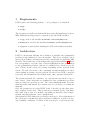
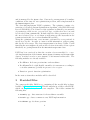
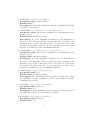
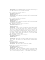
Parallel Optimization Workbench
(POW)
- User Manual -
Laboratory For Biomolecular Modeling, Institute of
Bioengineering, School of Life Sciences, Ecole Polytechnique
Fédérale de Lausanne - EPFL, Lausanne, Switzerland
Contents
1 Requirements
2
2 Architecture
2
3 Provided Files
4
4 Launching
5
5 Standard Keywords
6
6 Function Module
9
7 DockSymmCircle module
7.1 Overview . . . . . . . . . . .
7.2 Implementation Details . . .
7.2.1 Data Structures . .
7.2.2 Search Space . . . .
7.2.3 Fitness Function . .
7.2.4 Clustering . . . . . .
7.3 Keywords . . . . . . . . . .
7.4 Constraint File . . . . . . .
7.5 Parameterization Examples
.
.
.
.
.
.
.
.
.
.
.
.
.
.
.
.
.
.
8 Creation of a new POW Module
1
.
.
.
.
.
.
.
.
.
.
.
.
.
.
.
.
.
.
.
.
.
.
.
.
.
.
.
.
.
.
.
.
.
.
.
.
.
.
.
.
.
.
.
.
.
.
.
.
.
.
.
.
.
.
.
.
.
.
.
.
.
.
.
.
.
.
.
.
.
.
.
.
.
.
.
.
.
.
.
.
.
.
.
.
.
.
.
.
.
.
.
.
.
.
.
.
.
.
.
.
.
.
.
.
.
.
.
.
.
.
.
.
.
.
.
.
.
.
.
.
.
.
.
.
.
.
.
.
.
.
.
.
.
.
.
.
.
.
.
.
.
.
.
.
.
.
.
.
.
.
.
.
.
10
10
11
11
13
13
14
15
18
19
21
1
Requirements
POW requires the following python (>=2.5) packages to be installed:
• numpy
• mpi4py
The execution of parallel calculation will also require the installation of OpenMPI. Additonal packages may be required by specific POW modules:
• scipy, used by the modules DockDimer and DockSymmCircle
• MDAnalysis, used by the modules DockDimer and DockSymmCircle
• wxpython, required when running the GUI of the Function module
2
Architecture
POW is a framework allowing the resolution of virtually any optimization
problem via the addition of a specific module. This object oriented code is
developed in Python, and supports parellel computation by exploiting MPI
libraries. The architecture of our framework is represented in Figure 1. Every
box corresponds to a specific class. Classes highlighted in blue are common
to any optimization problem, and can be considered as a black box by the
user. Classes in the yellow area change depending on the problem being
solved. We will call module a file containing an implementation for these
classes aiming at solving a specific problem. In order to use POW, a user has
to provide two information: the module name, and a parameterization file.
The parameterization file contains a set of keywords associated to one or
more values. Some keywords are standard for any optimization problem,
whereas others are problem specific. The classes DefaultParser (for standard keywords) and Parser (for custom ones) are in charge of reading the
input file.
Once the parameters are parsed POW loads, if needed, specific data structures required by the user. This operation is performed by the class Data.
Since this class is part of a module, depending on how this class is implemented, any data structure can be manipulated.
Subsequently, POW defines the problem’s search space. Every dimension of
the search space is defined by upper and lower boundaries, as well as by specific boundary conditions. Creation of the search space is problem specific,
2
Default Parser
input
Parser
Default Space
Data
Space
Fitness
module
inertiaMax 0.9
inertiaMin 0.4
cp 1.2
cn 0.4
fitness fitness.py
boundaryMin 0.2 0.5 0.4
boundaryMax 5.1 4.6 9.4
…
PSO
Postprocess
result
Default Postprocess
Figure 1: Schematic of the Optimizer architecture. Every box represent a
class. Classes highlighted in blue are common to any optimization problem,
and can be considered as a black box for by the user. Classes in the yellow
area change depending on the problem being solved. We call a module a file
containing a definition for these classes aimed at solving a specific problem.
Input is provided as a text file containing keywords with associated values.
3
and is managed by the Space class. Converseley, management of boundary
conditions is the same for any optimization problem, and is implemented in
the DefaultSpace class.
The class PSO implements POW’s optimizer. The optimizer consists of a
variation of a Particle Swarm Optimization algorithm, called PSO Kick and
Reseed (PSO-KaR). The behavior of the optimizer is defined by an ensemble
of parameters called inertia, personal best (cp), neighborhood best (cn) and
kar threshold (kar_threshold). Default values for these parameters are set,
the user is however free to set them at will using specific keywords in the
parameterization file (see section Standard Keywords).
Along the optimization run, every measure performed by every particule is
stored in a log file. In order to extract useful information, postprocessing
this log file is necessary. The class Postprocess is in charge of this. Useful
functions the user might need, such as the selection of measures below a given
threshold, are preimplemented in the DefaultPostprocess class.
POW has been concieved so that the creation of a new module (i.e. a specific implementation of the Parser, Data, Space, Fitness and Postprocess
classes) is trivial even for a user unaware of its internal architecture. The
following modules are already available:
• DockDimer: dock two proteins into an heterodimer
• DockSymmCircle: rigid/flexible assembly of n monomers according to
a circular symmetry, possibly in presence of a receptor
• Function: generic function optimization
In the next sections these modules will be described.
3
Provided Files
The compressed folder POW.tar.gz containing all the needed files is downloadable at lbm.epfl.ch/resources. This file unpacks in a folder called POW,
which can be placed anywhere in your computer. The folder contains the
following files:
• Assembly.py : data structure for heterodimers assembly
• Default.py: classes common to any POW implementation
• DockDimer.py: dock two proteins
4
• DockSymmCircle.py: rigid/flexible assembly of n monomers according
to a circular symmetry, possibly around a given receptor
• Function.py: generic function optimization
• flexibility.py: functions for Principal Components Analysis
• parse.py: performs just the postprocessing, without running PSO.
This is useful when POW has been already run, and just alternate
postprocessing options on the produced results have to be tried. Usage
goes as follow:
./parse.py module input_file [logfile]
• POW.py: main executable
• Protein.py: PDB parser
• PSO.py: parallel implementation of Particle Swarm Optimization
4
Launching
POW is launched in the console by means of the following command:
mpiexec -n 4 $INSTALLATION_PATH/POW module input.dat
It is advised to create an alias, in order to make POW execution easier. The
following lines create a default call using 4 processors:
export NPROC=4
alias pow="mpiexec -n $NPROC $POW_DIR/POW.py"’
An execution becomes now as simple as:
pow module input.dat
This call will launch POW on 4 processors. A proper execution requires the
user to provide two arguments to the call: the desired optimization module
module and a parameterization file input.dat. The parameterization file
describes with a series of keywords how POW should behave. The input file
providing all the parametrisations for the search should be passed as parameter. The file is structured as a serie of keywords (one per line) having one or
more corresponding values. Keywords are case sensitive, and their order is
irrelevant. Some keywords are necessary for any kind of optimization procedure (see section ), whereas other are module specific (see sections dedicated
to specific modules). The # symbol can be used to comment out lines in
parameterization file.
5
5
Standard Keywords
The following keywords (implemented in Default.py) are typical to any
optimization problem, and are therefore accessible by any module:
• steps < number of steps to perf orm >
Acceptable values: positive integer
Default value: 100
Description: The number of steps that will be computed in the PSO.
• particles < number of particles >
Acceptable values: positive integer
Default value: 40
Description: The number of particles that will be used in each step
of the PSO.
• repeat < number of repetition >
Acceptable values: positive integer
Default value: 1
Description: Repeat can be used to lauch PSO multiple, consecutive
times. This is useful in order to enhance the sampling.
• repulsion < activate | desactivate >
Acceptable values: on | off
Default value: off
Description: When repulsion is activated, every good solution (solution smaller than filter_threshold, particle velocity converging to
zero) found by PSO will be flagged. Particles will be repelled by flagged
regions with a x−2 potential. When performing multiple PSO repetitions, flags are passed from one PSO run to the following one. This
enhances PSO sampling, since regions where a minima has been already
discovered are not oversampled. This option is currently experimental!.
• neighborType < type of neighbor >
Acceptable values: indexed | geographic
Default value: geographic
Description: NeighborType set the kind of neighborship between particles. In indexed neighborhood, particles are assigned an index, and
particles having consecutive indexes are considered as neighbots. In
geographic neighborhood, distance within particles in the search space
is considered.
6
• neighborSize < number of neighbor >
Acceptable values: positive integer
Default value: 1
Description: NeighborSize defines the amount of neighbors taken into
account by every particle.
• boundaryMin < min boundary f or each dimension >
Acceptable values: list of lower boundary for each dimension, separated by spaces.
Default value: module dependent
Description: It is the minimum boundary for each dimension of
the space. The first three values correspond to the rotations of the
monomer on x, y and z axis respectively. The last one is the value
specified by the radius keyword. In case you did not use the radius
keyword, you MUST specify a minimum radius here.
• boundaryMax < max boundary f or each dimension >
Acceptable values: list of upper boundary for each dimension, separated by spaces.
Default value: module dependent
Description: It is the maximum boundary for each dimension of
the space. The first three values correspond to the rotations of the
monomer on x, y and z axis respectively. The last one is the value
specified by the radius keyword. In case you did not use the radius
keyword, you MUST specify a maximum radius here.
• boundaryType < type of the boundary >
Acceptable values: 0 | 1
Default value: module dependent
Description: For each dimension it is possible to define the boundary condition. 0 and 1 stands for periodic and repulsive boundary
conditions respectively.
• inertiaMax < max inertia of particles >
Acceptable values: float 0-1
Default value: 0.9
Description: It is the maximum inertia of particles. Between steps of
the PSO the inertia is decreased until inertiaMin.
• inertiaMin < min inertia of particles >
Acceptable values: float 0-1
Default value: 0.4
7
Description: It is the minimum inertia of particles. Between steps of
the PSO the inertia is decreased until inertiaMin.
• cp < inf luence of local best solution >
Acceptable values: float
Default value: 1.2
Description: It is the influence on a particle of the best solution found
by that particle.
• cn < inf luence of global best solution >
Acceptable values: float
Default value: 1.4
Description: It is the influence on a particle of the best position found
by neighbors of that particle.
• kar_threshold < threshold f or kar execution >
Acceptable values: float > 0
Default value: 0.01
Description: When a particle is being slower than this threshold,
the kick and reseed procedure (KaR) will be triggered. The particle
will receive a random kick that will reaccelerate it. If, moreover, the
particle’s current fitness is smaller than filter_threshold, it will be also
reseeded in a random location. This avoids early convergence and forces
the swarm to explore further the search space. Notice that setting
kar_threshold to 0 disables KaR.
• filter_threshold < f itness value to accept >
Acceptable values: float
Default value: 0
Description: An ensemble of solution is found, but just some of these
will be good. This variable sets a threshold on the solutions fitness
function.
• output < text f ile >
Acceptable values: UNIX filename
Description: The text file will be used to store results.
• restart_freq < restrart writing f requency >
Acceptable values: int
Default value: round(steps/10)
Description: POW can automatically generate restart files saving
the swarm state. These can be used to restart the optimization process
after a crash. Setting this variable to −1 will disable restart writing.
8
• save_restart < restart saving f ile name >
Acceptable values: UNIX filename
Default value: swarm.restart
Description: Name of the restart file POW will automatically save
at a frequency given by restat_freq. The restart contains information about timestep, repetition, particles positions, velocities as well as
position and value of their respective current best solution. During execution, both the most recent restart and an older copy of it are stored
(default name swarm.restart.old)
• load_restart < restart loading f ile name >
Acceptable values: UNIX filename
Description: By providing a restart file, the optimization process will
restart from the last saved timestep and repetition. When restarting
an optimization, the original input file should not be changed (the
addition of load_restart statement is sufficient). The previous log file
will be backed up, and a new one will be generated. The new log file
will contain all the data of previous logfile recordered until the restart
point. If the old log file is not found, a new one is started.
6
Function Module
The Function module allows the minimization of any function not requiring
manipulation of any data structure. The file containing the fitness function
to be evaluated is passed to POW via the following keyword:
• fitness < f itness extraction f ile >
Acceptable values: UNIX filename
Default value: fit_multimer
Description: This file contains the implementation for the Fitness
class, and should have the following form:
class Fitness:
def __init__(self,data,params):
pass
def evaluate(self, num, pos):
#num: PSO particle index
#pos: array of particle’s position in search space
#compute fitness on the base of pos values
return fitness
9
The Function module can also be operated via a graphical interface invoked
with the command Function_GUI.py (see Figure 2). The interface allows
the user to create, edit and save a POW input file, validate it, and launch
a POW run on multiple processors. Notice that the use of this graphical
interface also requires the wxPython package to be installed.
Figure 2: POW graphical interface for Function module allowing the user
to save, edit, validate and launch POW input files.
7
7.1
DockSymmCircle module
Overview
With this POW module we aim at finding quickly a reasonable prediction
for a multimeric structure arrangement on the basis of structural information
about its subunits and experimental measures acting as search restraints. In
a first step, an ensemble of monomer conformations is generated, typically
from molecular dynamics simulations or structural biology experiments; this
will be treated as a conformational database (see Material and Methods).
The advantage of such an approach is that assembly prediction is performed
10
using physically plausible structures.
Upon definition of a list of geometric restraints and a specific symmetry, a
Particle Swarm Optimization (PSO) search subsequently tries to arrange the
elements of the conformational database in a multimeric assembly so that all
restraints are respected, and steric clashes avoided. Geometric restraints can
be typically provided by low resolution electron density maps or experiments
such as cross-linking disulfide scanning, mutagenesis or FRET. If necessary,
POW can assemble a multimer on a given substrate. At PSO search completion, a large set of solutions having a good score is usually generated. A
smaller set of representative solutions, typically less than ten, is returned by
clustering the accepted solutions according to their respective Root Mean
Square Deviation (RMSD).
At present, POW can predict hetero-dimers (when no symmetry is imposed,
i.e. addressing general protein-protein interactions) or homo-multimers with
or without a target substrate (if a circular symmetry is defined). This process
is usually very fast (less than 5 minutes on an average workstation, using 4
processors), and can produce small ensemble of solutions being sufficiently
good to generate biologically sound working hypotheses, and act as seeds for
further optimization steps using more computationally expensive techniques.
7.2
7.2.1
Implementation Details
Data Structures
In order to manipulate protein structures, two classes are implemented:
Protein and Multimer.
The Protein class allows to parse a PDB file, manipulate its coordinates,
and extract the coordinates of specific atom selections. If (instead of a simple
PDB file) an ensemble of structures is provided, POW will create a PDB
called protein.pdb which will be parsed and subsequently used as an index.
The ensemble of structures will be saved as a set of alternate coordinates. In
detail, the following methods are implemented:
• import_pdb(pdb): parse a PDB file
• coords=get_xyz(): get cartesian coordinates of every atom. Returns
a numpy N x3 array, where N is the number of atoms.
• set_xyz(coords): set cartesian coordinates of every atom. coords
must be a N x3 array, where N is the number of atoms.
11
• rotation(x,y,z): rotate the protein according to angles around the
x,y and z axis.
• r=rgyr(): compute gyration radius r
• c=center() compute geometric center c
• coords=atomselect(chain,resid,atom): get cartesian coordinates
of a subgroup of atoms selected by their chain name chain, residue
id resid and atom name atom. Returns a numpy M x3 array, where
M is the number of slected atoms. Chain, resid and atom can be also
a wildcard symbol "*" (selecting all atoms).
• write_pdb(outname): save a new PDB file.
Note that, in order to speedup the calculation and simplify data storage,
Protein stores a PDB as a numerical numpy array. Every chain name, atom
name and residue name are converted into a numerical equivalent using a
dictionnary.
The Multimer class is responsible of assemblying multimers on the base of an
initially given Protein object. At the moment, this class can just produce
multimers according to a circular symmetry. In detail, the following methods
are implemented:
• create_multimer(degree, radius, pos): creates a circular multimer composed of degree monomers, having an internal radius equal to
radius and having every monomer rotated according to pos=[x,y,z].
Notice that pos should be a numpy array. This is the first method to
call after initialization. A list of degree length of numpy arrays containing a copy or Protein coordinates is created. Subsequently, every
element in the list is individually manipulated to create a multimeric
arrangement.
• multimer_to_origin(): move the whole complex to the origin.
• z_to_origin(): move the complex to place its center of geometry at
z = 0.
• cords=atomselect(unit,chain,resid,atom): get cartesian coordinates of a subgroup of atoms selected by their unit id unit (numbering
of individual monomers counted clockwise), chain name chain, residue
id resid and atom name atom.
12
• w=get_width(): get multimer width w.
• h=get_height(): get multimer height h.
• d=distance(select1, select2): compute the minimal euclidean distance between two sets of points select1 and select2.
• coords=get_multimer_uxyz(): extract coordinates of all atoms in the
multimer, in a list of length N x3 numpy array, everz element of the list
being an arraz of monomer coordinates.
• coords=get_multimer_xyz(): extract coordinates of all atoms in the
multimer, appended in a unique numpy array.
• write_pdb(outname): save a new PDB file containing all the monomers
treated as chains of the same assembly.
7.2.2
Search Space
The conformational space of rigid assemblies having a circular symmetry is
defined by the three rotation angles (α, β, γ) of a single monomer with respect
of a center of symmetry aligned along the z axis, and a displacement r with
respect to it, which represents the radius of the assembly in its narrowest
point. If an ensemble of ligand structures is available, obtained for instance
from a MD simulation (or alternatively NMR or X-ray experiments), flexibility (or multiple conformations) can be introduced as set of further dimensions
in the search space. To do so, a principal component analysis (PCA) is initially performed on the ensemble. The projection value of every trajectory
frame along the most relevant eigenvectors, also called fluctuations, is computed. These are used as a way to index the trajectory frames, which we can
consider as a protein conformation database. This module can also flexibly
or rigidly assemble a multimeric complex around a rigid receptor. In this case
four additional degree of freedom, i.e. the translation of the whole assembly
along the z axis and the three rotations (φ, θ, ψ) of the receptor around itself.
In summary, the search space dimensions are (in order):
α, β, γ,r, z, φ, θ, ψ, eig_1, eig_2,...
7.2.3
Fitness Function
The fitness function scoring the quality of an assembly depends on two factors, geometry and energy. As geometric contribution, specific measures of
the current multimer m are compared to target values ~t being experimentally
13
known. The aim is to minimize the difference within the obtained and desired
values. Target measures can be as diverse as width or height obtained from
cryo-EM maps, to atomic distances obtained with FRET or cross-linking ex~ an ensemble of measures performed on a multimer. The
periments. Let c(m)
geometric score G(m) of a multimer is determined by the euclidean distance
within obtained and target measures:
q
~ · (~t − c(m))
~
G(m) = (~t − c(m))
(1)
In order to avoid steric clashes during assembly, a coarse energy potential is
also taken into account. This "minimalistic" contribution is constituted by
a 9-6 Lennard-Jones-type of potential describing all the Cα and Cβ atoms of
two neighboring monomers extracted from the assembly:
σ 9 σ 6
−
E(m) = 4
(2)
r
r
where r are all the distances within couples of atoms being at a distance
smaller than 12 Å, and = 1 and σ = 4.7. The values of these constants
correspond to the coarse-grained parameterization for Cα atoms in the Martini force field. The final fitness function f mixes geometric and energetic
contributions by means of the following weighted sum:
f (m) = c ∗ E(m) + (1 − c) ∗ G(m)
(3)
where c is a real value within 0 and 1. In our tests we set c = 0.2. After
preliminary tests, we found however that results are not sensitive to variations
of this value. The rough energy function in equation 2 only avoids clashed of
subunits, and at the current stage is not sufficiently precise to allow a blind
docking, i.e. a docking where no geometric restraints are provided. However,
work in the development of more accurate energy functions to be included
in the fitness function is currently ongoing. We expect this will enhance the
capabilities for the broad problem of protein-protein recognition.
7.2.4
Clustering
All fitness evaluations obtained during PSO are collected, and solutions having a fitness lower than a predefined threshold are retained. In most applications the filtering criteria is set to 0. Such a value indicates that, most likely,
the system’s energy is negative and geometric restraints are well respected.
Since several solutions usually represent similar conformations, clustering is
performed. Two ad hoc clustering approaches able to determine automatically the number of required clusters are available: the first groups solutions
14
being close enough in the search space (preimplemented in Default.py),
whereas the second clusters solutions generating assemblies having a small
RMSD within themselves. Cluster representatives are selected (cluster centers), ranked according to their fitness, and their corresponding assemblies
returned as an ensemble of PDB files.
7.3
Keywords
Additionally to default POW keywords 5, the following keywords are defined:
• radius < f ixed radius of the multimer >
Acceptable values: float
Description: use this keyword if you know precisely the multimer
internal radius in its narrowest point. If the precise radius is not known,
the user should define reasonable boundaries for the pore radius value
via the boundaryMin and boundaryMax keywords.
• degree < number of monomer >
Acceptable values: positive integer
Description: It is the number of monomer that compose the multimer.
• target < list of measures >
Acceptable values: list of float separated by spaces
Description: The list of target measure will be used by the system to
compute the fitness. This list MUST have the same schema as the list
computed from the constraint file.
• constraint < constraint f ile >
Acceptable values: UNIX filename
Description: The system generates a multimer corresponding to the
particle position in the space and passes it to the constraint file. See
the section 7.4 for details about the structure of this file. The list of
measure you return will be compared to the list of target’s measure
and output a fitness value that will be written to the output file. The
list of target measure MUST have the same order as the list of measure
computed in the constraint file.
• style < type of assembly >
Acceptable values: flexible | rigid
Default value: rigid
Description: Define the type of assembly to perform. If rigid is chosen, the monomer keyword must be defined as well. If flexible is chosen,
at least topology and trajectory keywords must be defined.
15
• monomer < monomer P DB f ile >
Acceptable values: UNIX filename
Description: PDB file containing the monomer. Requires style keyword set to rigid.
• trajectory < coordinates of a M D trajectory >
Acceptable values: path to a dcd or crd file
Description: Enesemble of protein structures. Requires style keyword
set to flexible.
• topology < topology of a M D trajectory >
Acceptable values: path to a charmm or amber topology
Description: Topology of provided trajectory (see trajectory keyword). Requires style keyword set to flexible.
• trajSelection < atom selection in M DAnalysis f ormat >
Acceptable values: MDAnalysis AtomSelect
Default value: protein
Description: Select a subset of atoms from provided trajectory. If
align keyword is set to yes, trajectory will also be aligned on this selection. PCA and subsequent assembly will only take these atoms into
account. Requires style keyword set to flexible.
• projection < projection of M D trajectory on main eigenvectors >
Acceptable values: path to a projections file
Description: If provided, Principal Components Analysis will not
be performed, and this file providing projections on main eigenvectors
will be used instead. This file should consist of a number of lines
matching the number of atoms in the provided trajectory, and a number
of columns corresponding to the desired number of eigenvectors used
for projection. Requires style keyword set to flexible.
• align < def ine whether to align the given trajectory >
Acceptable values: yes | no
Default value: yes
Description: If set to yes, the provided trajectory will be aligned on
the protein. Taken into account only if style keyword is set to flexible.
• ratio < energy represented by eigenvectors >
Acceptable values: float 0-1
Default value: 0.8
Description: After having performed PCA, POW selects a number
of representative eigenvector. These will represent at least a certain
16
percentage of the trajectory’s energy. Taken into account only if style
keyword is set to flexible.
• detectClash < clash detection switch >
Acceptable values: on, off
Default value: on
Description: define whether a 9-6 Lennard-Jones function should be
computed to assess the system’s energy.
• mixingWeight < weight energetic vs geometric contributions >
Acceptable values: float 0-1
Default value: 0.2
Description: fitness function is computed via the equation f = c ∗
energy + (1 − c ∗ distance), where c is the value of mixingWeight.
• receptor < clustering distance within solutions >
Acceptable values: UNIX filename
Description: PDB file containing a receptor around which the assembly will be built.
• z_padding < assembly vertical displacement >
Acceptable values: float > 0
Default value: 5
Description: the whole assembly is displaced along the z axis with
respect of the receptor. Boundary conditions are defined by a lower and
higher boundary. These are computed around the size of the receptor.
z_padding adds an additional dislacement to the computed boundaries.
Should be defined only if boundaryMinReceptor and boundaryMaxReceptor
are undefined, and if receptor is given.
• boundaryMinReceptor < min boundary f or receptor dimensions >
Acceptable values: list of lower boundary for each dimension, separated by spaces.
Default value: min_receptor-z_pad 0 0 -360/(2*degree)
Description: It is the minimum boundary for each dimension of
the space. The first three values correspond to the rotations of the
monomer on x, y and z axis respectively. The last one is the value
specified by the radius keyword. In case you did not use the radius
keyword, you MUST specify a minimum radius here.
• boundaryMaxReceptor < max boundary f or receptor dimensions >
Acceptable values: list of upper boundary for each dimension, separated by spaces.
17
Default value: max_receptor+z_pad 0 0 360/(2*degree)
Description: It is the maximum boundary for each dimension of
the space. The first three values correspond to the rotations of the
monomer on x, y and z axis respectively. The last one is the value
specified by the radius keyword. In case you did not use the radius
keyword, you MUST specify a maximum radius here.
• cluster_threshold < clustering distance within solutions >
Acceptable values:float > 0
Default value: 5
Description: Similar solutions will be clustered in a unique solution.
If RMSD clustering is chosen, a value smaller or equal to 5 Åis adviced.
If distance clustering is used, a number around 15 is suggested.
• output_folder < f older containing produced pdb structures >
Acceptable values:string
Default value: result
Description: POW will generate a set of pdb corresponding to the
clustering of best solutions. These, along with a summary file (solutions.dat) will be stored in the folder output_folder.
Note that the Default keywords boundaryMin and boundaryMax (see Default
keywords section 5) should include the following quantities in the following
order (see Search Space Definition and Data manipulation section 7.2.2):
α β γ radius
7.4
Constraint File
The constraint file is user provided, and contains a python function containing user defined measure on the generated multimer. In the absence of a
receptor, this script consists of one function accepting a Multimer object,
that must be declared as follows:
def constraint_check(multimer):
#user defined measures
return measure1 measure2
In case a receptor is also present in the optimization process, constraint_check
will have to accept two parameters, the second being the receptor (Protein
object)
The user can define various measures inside this function, and return them.
The return order is significant, it should indeed match the order of target
18
measures provided with the target keyword in input file. The multimer parameter is a Multimer object (see 7.2.1). This object provides the following
functions for measurement of the structure:
• multimer.get_width(), returns the assembly width
• multimer.get_height(), returns the assembly height
• multimer.atomselect(unit,chain,resid,name), returns a numpy 2D
array containing all the coordinates of atoms matching the selection.
• multimer.distance(a, b), returns the minimal euclidean distance
within two ensembles of points a and b (numpy 2D arrays, returned
for instance by the atomselect keyword)
7.5
Parameterization Examples
The minimal set of keywords for a POW parameterization file for protein
assembly are as follows:
monomer input.pdb
constraint constraint.py
degree 5
radius 10
target 10 20
This will rigidly assemble 5 monomers from file input.pdb so that the circular radius is 10. constraint.py file will be used as constraint. This file will
compute two measures, that should be compared with the target measures
10 and 20.
A complete example showing how to perform a rigid assembly is as follows:
steps 150
particles 50
repeat 3
boundaryMin 0 0 0 8
boundaryMax 360 180 360 12
assembly_style rigid
19
monomer protein.pdb
constraint constraint.py
degree 7
target 85 150
filter_threshold 0
cluster_threshold 5
In this example a calculation protocol with 150 iterations, 50 particles and
3 repetitions has been chosen. boundaryMin and boundaryMax keyword define a multimer with a radius varying from 8 to 12 Å. The provided monomer
(protein.pdb) will be treated as a rigid body, and assembled in a heptameric
structure (7-fold simmetry) being constrained by constrain.py function. In
postprocessing, only solutions having a fitness smaller than 0 will be retained,
and solutions having an RMSD smaller than 5 within themselves will be clustered.
By replacing the monomer keyword of previous example with what follows,
it’s possible to perform a flexible assembly.
style flexible
topology proten.prmtop
trajectory trajectory.dcd
align yes
ratio 0.80
Flexible assembly requires a trajectory (in crd or dcd format) and a topology
(pdb or psf). If the protein in the trajectory is not aligned, POW can do this
for you by means of the align keyword. This done PCA is performed on Cα
atoms. Notice that the number of degrees of freedom (3*N, where N is the
number of carbons) must be greater than the number of frames in the simulation. A number of eigenvectors representing more than 0.8 (80%) of the
system’s energy will be extracted and treated as protein’s degrees of freedom.
Aligning the trajectory and performing a PCA may take some time. However,
preprocessing phase, will generate an aligned trajectory (aligned.dcd) and
a file containing eigenvectors projection (proj_coordinates.dat). You can
20
indicate POW to use these file to avoid repeting the preprocessing. This can
be done in this way:
assembly_style flexible
topology proten.prmtop
trajectory aligned.dcd
align no
projection proj_coordinates.dat
8
Creation of a new POW Module
A module contains an implementation for Parser, Data, Space, Fitness and
Postprocess classes. The following lines represent a module skeleton.
from Default import Parser as R
from Default import Space as S
from Default import Postprocess as PP
#import other packages here
class Parser(P):
def __init__(self,infile):
#parse more params if needed
#see Default.py or DockSymmCircle.py for syntax
def check_variables(self):
#here you can perform consistency check on your parameters
class Data:
def __init__(self,params):
#load files previously parsed (contained in params object)
class Space(S):
def __init__(self,params,data):
#build search space using params and data objects defining:
#self.low = low boundaries
#self.high = high boundaries
#self.boundary_type = int array (0=periodic, 1=reflex)
21
class Fitness:
def __init__(self,data,params):
#load data here if needed (e.g. target measures,...)
def evaluate(self,num,pos):
#return fitness value
class Postprocess(PP):
def __init__(self,params,data):
#load params and data structure
def run(self):
#parse logfile and postprocess
22