Download Combining interval analysis with flatness theory

Combining interval analysis with flatness theory for
state estimation of sailboat robots
Luc Jaulin
Abstract. This paper proposes a new set-membership state estimator for estimating the state vector of a nonlinear dynamic robot. The method combines a symbolic technique based on flatness
concepts with rigorous numerical methods based on interval analysis. Two testcases related to the
state estimation of a sailboat robot are proposed to illustrate the principle and the efficiency of the
approach.
Keywords. bounded-error, constraint propagation, flatness, nonlinear observers, interval analysis,
sailboat, robotics, set theory.
ENSTA, LabSTICC, 2 rue François Verny
29806 Brest, France
Tel. +33 (0)2 98 34 89 10
web: www.ensta-bretagne.fr/jaulin/
1. Introduction
This paper presents a new interval approach for nonlinear state estimation with an application to
sailboat robotics. This problem is motivated by the microtransat challenge where small autonomous
sailboat robots are designed to cross the Atlantic ocean [5]. All components of such robots should
be as robust as possible with respect to all situations (heavy weather, waves, salt water, low level of
energy, long trip, . . . ). For sailboat robots, two types of sensors can be considered.
• Reliable sensors, which could survive under all situations. Such sensors are the GPS, the compass, the gyrometers and accelerometers. All these sensors are low energy consumers, can be
enclosed inside a waterproof tank and can survive for years. The GPS gives us the position of
the boat and new generation GPS can also return the speed of the boat with a good accuracy
by using the Doppler effect. Since magnetic perturbations inside the ocean can be neglected,
the compass measures the north direction with a rather good accuracy. The gyrometer returns
the rotational speed and the accelerometers provide the roll and pitch of the robot.
• Unreliable sensors, which have a high probability to brake down in case of heavy weather.
Anemometers (a device for measuring the wind speed), weather vane (to return the direction
of the wind), dynamometers which measure the forces on the sail or the rudder are considered
as unreliable. They are directly in contact with aggressive natural elements (wind, wave, salt)
and can fail at any time.
On the one hand, to control the robot, it is necessary to know where the wind comes from, its
power and the strength of the forces on the sail or on the rudder, if the mainsheet is tight or not, . . .
2
Luc Jaulin
(see e.g. [34], [19]). On the other hand, a reliable boat should only enclose reliable sensors. The aim
of this paper is twofold.
• The first goal is to show that the variables that could be measured by the unreliable sensors
could be reconstructed dynamically from the data collected by the reliable sensors. This is new
in a sailboat context, even if the possibility to control a sailboat robot without any wind sensor
has already been demonstrated in [38].
• The second goal is to give a new method which combines nonlinear symbolic observation techniques [9], based on flatness concepts, with interval analysis [31]. The first tool makes it possible to transform the observation problem into equations that have to be solved at each point
of time whereas interval analysis provides a systematic way to solve the inversion problem
[27] taking into account some interval uncertainties on the measured data. Combining interval
analysis with flatness has already been considered for control [16] or source separation [29],
but never for state estimation.
Section 2 shows how the state estimation problem can be transformed into a set inversion
problem parametrized by the time t. Basic notions on interval analysis and the set inversion algorithm
are both presented in Section 3. Section 4 presents the sailboat to be considered and illustrates the
procedure to be followed to transform the state estimation problem into a chain of set inversion
problems. Two simulated testcases are treated on Section 5. Section 6 concludes the paper.
2. Interval flatness approach for state estimation
This section shows how, using flatness theory, a state estimation problem can be cast into a sequence
of set inversion problems that have to be solved at each instant. Shortly speaking, flatness theory can
be seen as a symbolic computation approach to deal easily and efficiently with specific differential
equations. Consider the system described by the following state equations
x˙
y
= f (x, u)
= g(x),
(2.1)
where u ∈ Rm is the vector of controls (or the vector of actuators), x ∈ Rn is the state vector and
y ∈ Rm is the output vector (or sensors). The functions f and g are the evolution function and the
observation function, respectively. They are assumed to be as smooth as needed. The dimension of
u and that of y are assumed to be both equal to m. All vectors depend on the continuous time t. The
system is said to be flat with the flat output y if there exist two continuous functions φ and ψ and
integers r1 , . . . , rn such that for all t, we have

(rm −1)
 x = φ y1 , y˙ 1 , . . . , y (r1 −1) , . . . . . . , ym , y˙ m , . . . , ym
1
(2.2)
(rm )
 u = ψ y1 , y˙ 1 , . . . , y (r1 ) , . . . . . . , ym , y˙ m , . . . , ym
.
1
The integers ri correspond to the relative degrees for the outputs yj , j = 1, . . . , m. According to
Hermann and Krener [18], a system is observable if for any pair of state vector (xa , xb ), xa being
indistinguishable from xb implies xa = xb . Recall that a state vector xa is called indistinguishable
from xb , if for every admissible input u, they produce the same output. Now, from (2.2), two different states cannot produce the same output. We can conclude that all systems satisfying (2.2) are
observable: the function φ gives us the unique state vector which is consistent with the outputs and
their derivatives. Of course, we assume here that the output vector y is measured and that we can
estimate its derivatives with a good accuracy. In practice, the functions φ and ψ involved in (2.2) are
unknown. To get them, we have to proceed in two steps.
Combining interval analysis with flatness theory for state estimation of sailboat robots
(r )
3
(r )
• The derivation step (see [20]) computes symbolically y1 , y˙ 1 , . . . , y1 1 , . . . , ym , y˙m , . . . , ymm
as functions of x and u, using (2.1). We get an expression of the form


y1
 y˙1 
x


.
(2.3)
 ..  = h
u
 . 
(r )
ymm
This can be done automatically without any difficulty using symbolic computation. It suffices
to take all m equations yj = gj (x) and to compute symbolically its first, second, . . . rj th
derivatives with respect to t. At each step, the x˙ i are replaced by fi (x, u).
• The resolution step inverses symbolically the function h to get an expression of the form (2.2).
This operation is difficult to obtain except for simple systems.
Example 1. Consider the system

 x˙ 1 = x1 + x2
x˙
= x22 + u
 2
y
= x1 .
For the derivation step, we compute y, y,
˙ y¨ with respect to x and u. We get

 y = x1
y˙ = x˙ 1 = x1 + x2

y¨ = x˙ 1 + x˙ 2 = x1 + x2 + x22 + u.
Thus


x1
.
x1 + x2
h
=
2
x1 + x2 + x2 + u
For the resolution step, we have to isolate x, u to get an expression with respect to y, y,
˙ y¨. We get

 x1 = y
x2 = y˙ − x1 = y˙ − y

u = y¨ − x1 + x2 + x22 = y¨ − y˙ − (y˙ − y)2 .
x
u
As a consequence,

y
 φ (y, y)
˙
=
y˙ − y

ψ (y, y,
˙ y¨) = y¨ − y˙ − (y˙ − y)2 .
Note that here, the relative degree is r = 2.
Equation (2.3) can be rewritten as
z = h (w) ,
(2.4)
where
z =
w =
(r1 )
y1 , y˙ 1 , . . . , y1
T T
xT , u
.
(rm )
, . . . . . . , ym , y˙m , . . . , ym
and
(2.5)
(2.6)
Assumption. We assume that for all variables involved in Equation (2.4), membership intervals are
available [37]. These intervals can either be punctual if the value of the corresponding variable is
known, small if the variable is measured with good accuracy or equal to ] − ∞, ∞[ if nothing is
known about the variable. For our state estimation problem, we have three types of variables.
4
Luc Jaulin
• The input variables uj , j ∈ {1, . . . , m} can be assumed to be known exactly or with a good
precision, i.e., the corresponding interval [uj ] can be assumed to be small or punctual.
(k)
• The derivatives yj of the output variables yj , j ∈ {1, . . . , m}, k ∈ {0, . . . , rj }, are measured
(k)
with a known error. The intervals yj
(k)
containing yj
can be considered as small. For robotic
(k)
applications, the intervals for derivatives yj can often be obtained directly via derivativebased sensors (such as loch-Doppler systems, gyrometers or accelerometers). When no such
sensor is available and when the signals yj are not too noisy, a robust differentiation method
(k)
(see e.g. [30]) can provide an estimate for the derivatives yj (but without any estimation of the
(k)
error). This estimation might help the user to get intervals yj , but without any reliability.
• The state variables xi , i ∈ {1, . . . , n} are considered as unknown. The corresponding intervals
[xi ] are thus ] − ∞, ∞[.
Define the boxes
[w] = [x1 ] × · · · × [xn ] × [u1 ] × · · · × [um ],
[x]
[u]
and
(r1 )
[z] = [y1 ] × [y˙ 1 ] × · · · × y1
(rm )
× . . . · · · × [ym ] × [y˙ m ] × · · · × ym
.
The posterior feasible set for w is
W = {w ∈ [w] , ∃z ∈ [z] , z = h (w)}
= [w] ∩ h−1 ([z]) .
(2.7)
Characterizing the set W for a given t is thus a set inversion problem [27] which can be solved
efficiently using interval analysis. Once W has been computed, the posterior feasible set X for x is
easily obtained by a projection of W onto the x-space.
(k)
Remark 1. If the system is flat, it is observable [6], [12], i.e., if the quantities yj , k ≤ rj −
1, j ∈ {1, . . . , m} are known without any error, then the set X(t) is a singleton. This is a direct
(k)
(k)
consequence of the relations (2.2). In this paper, we only know intervals yj
enclosing the yj .
As a consequence, the set X(t) generally encloses an infinite number of elements. However, its size
can be small enough to allow us to find a control that fits to all state vectors inside X(t).
Remark 2. When the system is flat, we may already have an analytical expression for h−1 and
thus interval methods are not required anymore for the inversion. Now, for our sailing boat or for
many other engineering systems, the inversion cannot be done symbolically and a reliable inversion
procedure, such as that provided by interval set inversion [27], is necessary.
Remark 3. When m
i=1 ri > n, the inversion problem is overdetermined and the functions φ
and ψ are not unique. Equivalently, if m
i=1 ri > n, the dimension of the set to be inverted (equal to
m
(r
+
1))
is
larger
than
the
number
of unknowns (equal to n + m). This is a problem for most
i=1 i
symbolic methods but not for the set inversion approach.
3. Set inversion with interval analysis
With an interval approach, a random variable x ∈ R is represented by an interval [x] which encloses
the support of its probability function. This representation is of course poorer than that provided
by its probability density distribution, but it presents several advantages. (i) Since an interval with
non-zero length is consistent with an infinite number of probability distribution functions, an interval representation is well adapted to represent random variables with imprecise probability density
functions. (ii) An arithmetic can be developed for intervals, which makes it possible to deal with
Combining interval analysis with flatness theory for state estimation of sailboat robots
5
uncertainties in a reliable and easy way, even when strong nonlinearities occur. (iii) When the random variables are related by constraints (i.e., equations or inequalities) a propagation process (which
will be explained later) provides an efficient polynomial algorithm that computes intervals enclosing
all feasible values for the random variables. Interval analysis is used for robotics applications when
strong nonlinearities are involved in the formulation of the problem. See, e.g., [26] for control, [7]
and [28] for estimation and also [14] in the context of sailboat robotics.
3.1. Interval arithmetic
An interval is a closed and connected subset of R. Consider two intervals [x] and [y] and an operator
⋄ ∈ {+, −, ·, /}, we define [x] ⋄ [y] as the smallest interval which contains all feasible values for
x ⋄ y, if x ∈ [x] and y ∈ [y] (see [31]). For instance
[−1, 3] + [2, 5] = [1, 8],
[−1, 3] · [2, 5] = [−5, 15],
[−1, 3]/[2, 5] = [− 12 , 32 ].
If f is an elementary function such as sin, cos, . . . we define f([x]) as the smallest interval which
contains all feasible values for f (x), if x ∈ [x].
3.2. Contractors
Consider a constraint C (i.e., an equation or an inequality), some variables x1 , x2 , . . . involved in
C and prior interval domains [xi ] for the xi ’s. Interval arithmetic makes it possible to contract the
domains [xi ] without removing any feasible values for the xi ’s. A contraction operator is called
a contractor. When several constraints are involved, contractors are called sequentially, until no
more significant contraction can be observed (see [3], [36], [25], for more details). The interval
propagation method converges to a box which contains all solutions of our set of constraints. If this
box is empty, it means that there is no solution. It can be shown that the box toward which the
method converges does not depend on the order with which the contractors are applied [1], but the
computing time is highly sensitive to this order. There is no optimal order in general, but in practice,
one of the most efficient is called forward-backward propagation. It consists in writing the equation
in the form y = h (x). Then, using interval arithmetic, the intervals are propagated from x to y in
a first step (forward propagation) and, in a second step, the intervals are propagated from y to x
(backward propagation). The principle can be extended to problems involving quantifiers as shown
in [33].
3.3. Algorithm for set inversion
We now present an algorithm [27] to characterize the set W = [w] ∩ h−1 ([z]), as required by
Equation (2.7). The corresponding algorithm is given by the table below. The inputs of this algorithm
are [w] which is a (possibly huge) box enclosing all feasible w = (x, u) for all t and [z] is the box
(j)
(j)
defined as the Cartesian product of the intervals yi
enclosing the outputs yi of our system at
time t (see Equation (2.5)). The set W+ is a subpaving (i.e., a union of boxes) which encloses the
feasible set W.
6
Luc Jaulin
Algorithm S IVIA (in: [w], [z], out: X+ )
1 L := {[w]}
2 repeat
3
pull ([w], L) ;
4
while the contractions are significant
5
compute [w]
¯ enclosing [w] ∩ h−1 ([z])
6
end repeat
7
bisect [w]
¯ and push the resulting boxes into L
8 until all boxes of L have a width smaller than ε
9 W+ := ∪L.
The list L contains boxes, the union of which encloses W. It is initialized at Step 1 with the
single box [w]. At Step 2, a repeat-until loop is run until all boxes of L have a width smaller than
a given accuracy ε, which is chosen small enough to have a good accuracy on the result and large
enough to respect the allowed computing time. At Step 3, the largest box is pulled out from the list.
The forward-backward contractor is iterated at Step 4 until no more significant contraction can be
observed, i.e., until the Hausdorff distance between the current box and the contracted box is smaller
than a given threshold. At Step 7, the current box [w]
¯ is bisected into two smaller boxes. These two
boxes are pushed at the end of the queue L. At Step 9, the algorithm returns the subpaving W+
made by the union of all boxes stored in L. The properties of S IVIA (time and space complexity,
convergence, . . . ) have been studied in [27]. The complexity has been shown to be exponential with
respect to the dimension of w.
4. State estimator for the sailboat
4.1. Model used by the state estimator
The application to be considered in this paper is the estimation of the state of a sailboat in order to
reconstruct the force and the direction of the wind. Three types of models are generally considered
when dealing with robotics applications. They are listed now with an increasing degree of fidelity.
• The model for the controller. It should be as simple as possible (if possible linear) in order to
be able to control the robot in a robust way. For instance, if one uses a proportional–integral–
derivative (PID) controller to control the heading of a sailboat, the underlying model that is
assumed is a second-order linear system, which behaves approximately as a sailboat (in a
control point of view).
• The model for the state estimator. It should also be simple but should behave approximately
as the actual robot. This model should take into account the nonlinearities of the robot and the
nature of the noise.
• The model for the simulator. It should be as realistic as possible taking into account the environment (the swell, interaction with other boats, . . . ), the sensors, the actuators, the communication, . . . [11], [15]. As a consequence, it is generally complex and non-deterministic.
We shall propose a simple deterministic model that will be assumed by our state estimator
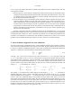
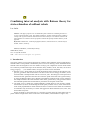
to describe the dynamics of the sailboat (see Figure 1). This model is given by the following state
Combining interval analysis with flatness theory for state estimation of sailboat robots
equations





















x˙
y˙
θ˙
v˙
ω˙
a˙
ψ˙
fs
fr
γ



















 δs
=
=
=
=
=
=
=
=
=
=
=
7
v cos θ + p1 a cos ψ
v sin θ + p1 a sin ψ
ω
fs sin δ s −fr sin u1 −p2 v2
p9
fs (p6 −p7 cos δ s )−p8 fr cos u1 −p3 ω
p10
0
0
p4 a sin (θ − ψ + δ s )
p5 v sin u1
cos (θ − ψ) + cos (u2 )
π−θ+ψ
if γ ≤ 0
sign (sin (θ − ψ)) · u2 otherwise
(4.1)
where p1 is the drift coefficient, p2 is the tangential friction, p3 is the angular friction, p4 is the
sail lift, p5 is the rudder lift, p9 is the mass of the boat and p10 is its mass moment of inertia. The
distances p6 , p7 , p8 are represented in Figure 1. All parameters pi are assumed to be known exactly.
The sailboat has two inputs: u1 = δ r is the angle between the rudder and the sailboat and u2 = ¯δ s
is the maximum angle of the sail (which is limited by the length of the mainsheet). This model is
similar to that described in [23], [22], except that here, (i) we added the direction of the wind ψ and
its amplitude a as state variables and (ii) the control is not anymore the sail angle, but the length of
the mainsheet, which is more realistic.
To apply the method proposed in Section 2, the model has to be deterministic. This is why we
assumed that wind properties are piecewise constant by taking a˙ = ψ˙ = 0. We can also allow some
small variations of the wind by replacing a˙ = ψ˙ = 0 by a˙ = u3 , ψ˙ = u4 , where the intervals for the
two new inputs u3 , u4 correspond to the feasible wind perturbations. The sailboat model has been
chosen in order to illustrate the new state estimation approach developed in this paper. The strong
nonlinearities of this model, its hybrid behavior (due to the fact that the mainsheet may be tight or
not) make the estimation problem very difficult to solve using existing approaches. However, it can
be easily solved by the presented approach. Now this model for the sailboat could be made more
realistic by adapting the modeling tools described by Fossen in the context of marine vessel [10] to
sailboats.
4.2. State estimator
˙
The state estimator to be proposed is based on the previous model and assumes that x, y, θ, x,
˙ y,
˙ θ,
x
¨, y¨, ¨θ are known with a given error. This assumption is rather realistic if our robot is equipped with
a Doppler GPS and accelerometers. Otherwise, robust differentiation methods should be considered
˙ ¨θ. From the state equations of the model, it is easy to check that
[30] to get x,
˙ y,
˙ x
¨, y¨, θ,




x
x
 y 
 y 




 θ 
 θ 




 x˙ 
 v 




 y˙  = h ω  ,




 θ˙ 
 a 




 x

 ψ 
 ¨ 


 y¨ 
 u1 
¨θ
u2
z
w
8
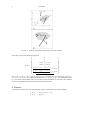
Luc Jaulin
F IGURE 1. Sailboat considered to illustrate the new state estimator
where h is given by the following expression








h (w) = 







x
y
θ
v cos θ + p1 a cos ψ
v sin θ + p1 a sin ψ
ω
(fs sin δs −fr sin u1 −p2 v2 ) cos θ
− ωv sin θ
p9
(fs sin δs −fr sin u1 −p2 v2 ) sin θ
+ ωv cos θ
p9
fs (p6 −p7 cos δs )−p8 fr cos u1 −p3 ω
p10
















and fs (w) , fr (w) , δ s (w) , γ (w) are given by (4.1). From the box [z] enclosing the vector z =
˙ x
(x, y, θ, x,
˙ y,
˙ θ,
¨, y¨, ¨θ)T , we compute the feasible set W = [w] ∩ h−1 ([z]). The Tchebychev center
(i.e., the center of the smallest cube W) provides us with an estimate for the state vector and thus
serves as an estimation for the direction and the speed of the wind.
5. Testcases
To illustrate the behavior of our state estimator, assume that the actual robot is described by
x˙ (t) = f (x (t) , u (t)) + ε (t)
y (t) = g(x (t)),
Combining interval analysis with flatness theory for state estimation of sailboat robots
9
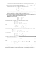
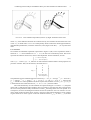
F IGURE 2. Left: simulated experiment (Testcase 1); Right: estimation of the wind
where ε (t) is the difference between the evolution used by our estimator and the actual robot. The
vector ε (t) is called model error. It is a small quantity which encloses the model approximations,
unpredictable perturbations (variations of the wind, swell, algae on the keel, . . . ) or any other state
noise.
5.1. Testcase 1
We consider the simulated experiment represented in Figure 2 (left). In this experiment which is
started at t0 = 0 and terminated at tmax = 17 s, the boat was controlled by hand. The arrows
represent the unknown wind vector, which is time dependent. For the simulation, we took
a˙ = 0.2 cos (0.1t)
ψ˙ = −0.1 sin (0.1t)
(5.1)
with a (0) = 10 and ψ (0) = 2, whereas our state estimator assumes that the wind properties are
piecewise constant. Thus, for this testcase, the model error is


0


0




0



.
0
ε(t) = 



0


 0.2 cos (0.1t) 
−0.1 sin (0.1t)
The parameters for the simulation have been chosen as p1 = 0.1, p2 = 100 kg·s−1 , p3 = 500 N·m·s,
p4 = 500 kg·s−1 , p5 = 70 kg·s−1 , p6 = 1.1 m, p7 = 1.4 m, p8 = 2 m, p9 = 1000 kg and
˙ x
p10 = 2000 N·m·s2 . These parameters are known by the state estimator. For all x, y, θ, x,
˙ y,
˙ θ,
¨, y¨, ¨θ
−3
−3
a small uniform noise inside the interval [−2 · 10 , 2 · 10 ] has been added.
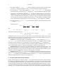
The results obtained by our state estimator are represented Figure 3. At time t0 = 0, the speed
of the boat is small and the state estimator does not provide a good precision due to the fact that
the set inversion problem is badly conditioned. At time t1 , the tuning of the sail is not optimal. As a
consequence, we have two ambiguous solutions for the sail (either the sail is too closed or it is too
open) which produce the same result. At time t4 the wind come from the back and it is not possible
to guess if the sail is on the right or on the left. Inside the interval [t2 , t3 ], we have γ ≤ 0, the boat
10
Luc Jaulin
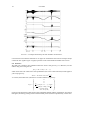
F IGURE 3. Envelopes obtained by the state estimator for Testcase 1.
is thus head to wind and the mainsheet is not tight. We checked that the interval envelopes always
contain the true signals. Figure 2 (right) represents on the world frame all feasible wind vectors.
5.2. Testcase 2
We shall now consider a new simulation where the wind is still given by (5.1). However, we also
added a drag force along the sail
fdrag = 30 a cos(θ + δ v − ψ)
which slows down the robot and a swell perturbation (the waves come from East) which applies a
yaw torque given by
t
Tswell = 30 sin θ cos θ cos 10
.
As a result, the model error (unknown to our state estimator) is given by


0


0




0
 30


a
cos(θ
+
δ
−
ψ)
cos
δ
ε(t) =  p9
v
v 
.
 30 sin(θ) cos(θ) cos( t ) 

 p10
10


0.2 cos (0.1t)
−0.1 sin (0.1t)
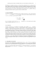
Figure 4 (left) depicts the actual motion of the simulated sailboat with the perturbation. Note that in
this figure, the tacking (turning between starboard and port tack) has been perturbed by a swell wave.
Combining interval analysis with flatness theory for state estimation of sailboat robots
11
F IGURE 4. Left: simulated experiment (Testcase 2); Right: estimation of the wind
F IGURE 5. Envelopes obtained by the state estimator for Testcase 2;
The results provided by the state estimation are depicted in Figure 4 (right) and Figure 5. Most of
the time, the true signals (painted grey) are inside the envelope (painted black) provided by the state
estimator. When it is not the case, we observe that these true signals are close to the envelope. The
fact that the envelopes do not always enclose the true signals is due to the unmodelled behaviors: the
interval resolution considers that there exist no drag force and no swell perturbation.
12
Luc Jaulin
Note that the model we have used for the simulation should be made more realistic to validate
our state estimator. This could be done by building an accurate model using recent ship modelling
techniques (see e.g. [4], [17], [2]).
The C++ code of the simulation as well as movies illustrating the simulated experiments with
the interval state estimator can be downloaded at
www.ensta-bretagne.fr/jaulin/getwind.html
6. Conclusions
This paper has presented a new approach for nonlinear state estimation. This approach combines
some nonlinear state estimation techniques [9] based on flatness [8] with interval set inversion. Flatness makes it possible to transform the state estimation problem in a symbolic way into set inversion
problems parametrized by the time t. Interval analysis solves numerically, rigorously and efficiently
the resulting set estimation problems for each t. The resulting state estimator has several advantages
over classical approaches.
• The state estimator is reliable with respect to nonlinearities. Thanks to interval analysis, it
is able to deal with nonlinear (or nondifferentiable and even noncontinuous) state equations,
without linearizing (as done by the extended Kalman filter [35]) or approximating them.
• The state estimator does not require the interval integration of differential equation. Such integrations are needed by all other interval state estimation methods [21], [24], [32], [13] which
makes them inefficient for high-dimensional systems.
• The state estimator takes into account bounded noise on the outputs and their derivatives. To
my knowledge, it is not done by existing algebraic nonlinear state estimators.
• The state estimator can be used for real-time applications. For each t, interval set inversion has
solved the state estimation of our sailboat problem within a time smaller than 0.1 sec.
The approach has been illustrated on the state estimation of a sailboat. The sailboat estimation
problem has several advantages: (i) it is motivated by the fact that we want to build a reliable boat
without unreliable sensors, (ii) it is simple enough to illustrate the principle and the generality of
presented approach and (iii) it is difficult enough to make all existing other deterministic nonlinear
approaches for state estimation fail.
References
[1] K. Apt. The essence of constraint propagation. Theoretical Computer Science, 221(1-2):179–210, 1998.
[2] A. Behal, B.M. Dawson, W.E. Dixon, and Y. Fang. Tracking and regulation control of an underactuated
surface vessel with nonintegrable dynamics. IEEE Transactions on Automatic Control, 47(3):495–500,
2002.
[3] F. Benhamou, F. Goualard, L. Granvilliers, and J-F. Puget. Revising Hull and Box Consistency. In ICLP,
pages 230–244, 1999.
[4] V. Bertram. Practical Ship Hydrodynamics. F. Vieweg & Sohn, Butterworth - Heinemann, 2000.
[5] Y. Brière. The first microtransat challenge, http://web.ensica.fr/microtransat. ENSICA,
2006.
[6] S. Diop and M. Fliess. Nonlinear observability, identifiability and persistent trajectories. In Proc. 36th
IEEE Conf. Decision Control, pages 714–719, Brighton, 1991.
[7] V. Drevelle and P. Bonnifait. High integrity gnss location zone characterization using interval analysis. In
ION GNSS, 2009.
[8] M. Fliess, J. Lévine, P. Martin, and P. Rouchon. Flatness and defect of non-linear systems: introductory
theory and applications. International Journal of Control, (61):1327–1361, 1995.
Combining interval analysis with flatness theory for state estimation of sailboat robots
13
[9] M. Fliess and H. Sira-Ramirez. Control via state estimations of some nonlinear systems. In Proc. Symp.
Nonlinear Control Systems (NOLCOS 2004), Stuttgart, 2004.
[10] T. Fossen. Guidance and Control of Ocean Vehicles. Wiley, New York, NY, 1995.
[11] T.J. Gale and J.T. Walls. Development of a sailing dinghy simulator. Simulation, 74(3):167–179, 2000.
[12] J.P. Gauthier and I. Kupka. Deterministic observation theory and applications. Cambridge University
Press, 2001.
[13] A. Gning and P. Bonnifait. Constraints propagation techniques on intervals for a guaranteed localization
using redundant data. Automatica, 42(7):1167–1175, 2006.
[14] A. Goldsztejn and L. Jaulin. Inner and outer approximations of existentially quantified equality constraints.
In Proceedings of the Twelfth International Conference on Principles and Practice of Constraint Programming, (CP 2006), Nantes (France), 2006.
[15] G. Guillou. Architecture multi-agents pour le pilotage automatique des voiliers de compétition et extensions algébriques des réseaux de Petri. PhD dissertation, Université de Bretagne, Brest, France, 2011.
[16] V. Hagenmeyer and E. Delaleau. Robustness analysis of exact feedforward linearization based on differential flatness. Automatica, (39):1941–1946, 2003.
[17] H. Hansen, P.S. Jackson, and K. Hochkirch. Real-time velocity prediction program for wind tunnel testing
of sailing yachts. In International Conference on the Modern Yacht, Southampton, 2003.
[18] R. Hermann and A. J. Krener. Nonlinear controllability and observability. IEEE Transactions on Automatic
Control, 22(5):728–740, October 1977.
[19] P. Herrero, L. Jaulin, J. Vehi, and M. A. Sainz. Guaranteed set-point computation with application to the
control of a sailboat. International Journal of Control Automation and Systems, 8(1):1–7, 2010.
[20] A. Isidori. Nonlinear Control Systems: An Introduction, 3rd Ed. Springer-Verlag, New-York, 1995.
[21] L. Jaulin. Nonlinear bounded-error state estimation of continuous-time systems. Automatica, 38:1079–
1082, 2002.
[22] L. Jaulin. Modélisation et commande d’un bateau à voile. In CIFA2004 (Conférence Internationale Francophone d’Automatique), In CDROM, Douz (Tunisie), 2004.
[23] L. Jaulin. Représentation d’état pour la modélisation et la commande des systèmes (Coll. Automatique de
base). Hermès, London, 2005.
[24] L. Jaulin, M. Kieffer, I. Braems, and E. Walter. Guaranteed nonlinear estimation using constraint propagation on sets. International Journal of Control, 74(18):1772–1782, 2001.
[25] L. Jaulin, M. Kieffer, O. Didrit, and E. Walter. Applied Interval Analysis, with Examples in Parameter and
State Estimation, Robust Control and Robotics. Springer-Verlag, London, 2001.
[26] L. Jaulin, S. Ratschan, and L. Hardouin. Set computation for nonlinear control. Reliable Computing,
10(1):1–26, 2004.
[27] L. Jaulin and E. Walter. Guaranteed nonlinear parameter estimation via interval computations. Interval
Computation, pages 61–75, 1993.
[28] L. Jaulin, E. Walter, O. Lévêque, and D. Meizel. Set inversion for χ-algorithms, with application to guaranteed robot localization. Mathematics and Computers in Simulation, 52(3-4):197–210, 2000.
[29] S. Lagrange, L. Jaulin, V. Vigneron, and C. Jutten. Nonlinear blind parameter estimation. IEEE Transactions on Automatic Control, 53(4):834–838, 2008.
[30] M. Mboup, C. Join, and M. Fliess. A revised look at numerical differentiation with an application to nonlinear feedback control. In The 15th Mediterranean Conference on Control and Automation - MED’2007,
2007.
[31] R. E. Moore. Methods and Applications of Interval Analysis. SIAM, Philadelphia, PA, 1979.
[32] T. Raissi, N. Ramdani, and Y. Candau. Set membership state and parameter estimation for systems described by nonlinear differential equations. Automatica, 40:1771–1777, 2004.
[33] S. Ratschan. Uncertainty propagation in heterogeneous algebras for approximate quantified constraint
solving. Journal of Universal Computer Science, 6(9):861–880, 2000.
[34] C. Sauze and M. Neal. An autonomous sailing robot for ocean observation. In proceedings of TAROS 2006,
pages 190–197, Guildford, UK, 2006.
14
Luc Jaulin
[35] S. Thrun, W. Bugard, and D. Fox. Probabilistic Robotics. MIT Press, Cambridge, M.A., 2005.
[36] M. van Emden. Algorithmic power from declarative use of redundant constraints. Constraints, 4(4):363–
381, 1999.
[37] E. Walter and L. Pronzato. Identification of Parametric Models from Experimental Data. Springer-Verlag,
London, UK, 1997.
[38] K. Xiao, J. Sliwka, and L. Jaulin. A wind-independent control strategy for autonomous sailboats based on
voronoi diagram. In CLAWAR 2011 (best paper award), Paris, 2011.
Luc Jaulin
e-mail: [email protected]