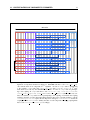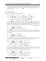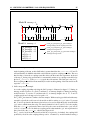
1
OASIS3-MCT User Guide OASIS3-MCT 3.0 Edited by: S. Valcke, T. Craig, L. Coquart CERFACS/CNRS SUC URA No1875 CERFACS TR/CMGC/15/38 May 2015 Copyright Notice c Copyright 2015 by CERFACS All rights reserved. No parts of this document should be either reproduced or commercially used without prior agreement by CERFACS representatives. How to get assistance? Assistance can be obtained as listed below. Phone Numbers and Electronic Mail Adresses Name Phone Affiliation e-mail Laure Coquart CNRS oasishelp(at)cerfacs.fr Sophie Valcke CERFACS How to get documentation ? The documentation can be downloaded from the OASIS web site under the URL : http://oasis.enes.org Contents 1 2 3 4 5 Introduction 1.1 Step-by-step use of OASIS3-MCT . . . . . . . . . . . 1.2 OASIS3-MCT sources . . . . . . . . . . . . . . . . . 1.3 Licenss and Copyrights . . . . . . . . . . . . . . . . . 1.3.1 OASIS3-MCT license and copyright statement 1.3.2 MCT copyright statement . . . . . . . . . . . 1.3.3 The SCRIP 1.4 license copyright statement . . . . . . . . . . . . . . . . . . . . . . . . . . . . . . . . . . . . . . . . . . . . . . . . . . . . . . . . . . . . . . . . . . . . . . . . . . . . . . . . . . . . . . . . . . . . . . . . . . . . . . . . . . . . . . . . . . . . 2 3 3 5 5 5 6 Interfacing a component code with OASIS3-MCT 2.1 Configurations of components supported . . . . . . . . . 2.2 OASIS3-MCT Application Programming Interface (API) 2.2.1 Module to use in the code . . . . . . . . . . . . 2.2.2 Initialisation . . . . . . . . . . . . . . . . . . . 2.2.3 Partition definition . . . . . . . . . . . . . . . . 2.2.4 Grid data file definition . . . . . . . . . . . . . . 2.2.5 Coupling field declaration . . . . . . . . . . . . 2.2.6 End of definition phase . . . . . . . . . . . . . . 2.2.7 Sending “put” and receiving “get” actions . . . . 2.2.8 Termination . . . . . . . . . . . . . . . . . . . . 2.2.9 Auxiliary routines . . . . . . . . . . . . . . . . 2.3 Coupling algorithms - LAG and SEQ concepts . . . . . . 2.3.1 The lag concept . . . . . . . . . . . . . . . . . . 2.3.2 The sequence concept . . . . . . . . . . . . . . . . . . . . . . . . . . . . . . . . . . . . . . . . . . . . . . . . . . . . . . . . . . . . . . . . . . . . . . . . . . . . . . . . . . . . . . . . . . . . . . . . . . . . . . . . . . . . . . . . . . . . . . . . . . . . . . . . . . . . . . . . . . . . . . . . . . . . . . . . . . . . . . . . . . . . . . . . . . . . . . . . . . . . . . . . . . . . . . . . . . . . . . . . . . . . . . . . . . . . . . . . . . . . . . . . . . . . . . . . . . . . . . . . . . . . . . . . . . . . . . . . . . . . . . . . . . 7 7 10 10 10 12 16 17 18 18 20 21 23 23 26 The configuration file namcouple 3.1 An example of a simple namcouple . . . . . . . . . . . . . . . . . . . . . 3.2 First section of namcouple file . . . . . . . . . . . . . . . . . . . . . . . 3.3 Second section of namcouple file . . . . . . . . . . . . . . . . . . . . . 3.3.1 Second section of namcouple for EXPORTED and EXPOUT fields 3.3.2 Second section of namcouple for OUTPUT fields . . . . . . . . . 3.3.3 Second section of namcouple for INPUT fields . . . . . . . . . . . . . . . . . . . . . . . . . . . . . . . . . . . . . . . . . . . . . . . . . . . . . . . . . . . . . . . . 27 27 29 30 30 31 32 Transformations and interpolations 4.1 Time transformations . . . . . . . . . . . . . . 4.2 The pre-processing transformations . . . . . . 4.3 The remapping (or interpolation or regridding) . 4.4 The post-processing stage . . . . . . . . . . . . . . . . . . . . . . . . . . . . . . . . . . . . . . . . . . . . . . . . 33 33 34 34 38 . . . . . . . . . . . . . . . . . . . . . . . . . . . . . . . . . . . . . . . . . . . . . . . . . . . . . . . . OASIS3-MCT auxiliary data files 40 5.1 Grid data files . . . . . . . . . . . . . . . . . . . . . . . . . . . . . . . . . . . . . . . . . 40 5.2 Coupling restart files . . . . . . . . . . . . . . . . . . . . . . . . . . . . . . . . . . . . . 41 ii CONTENTS 5.3 5.4 6 Input data files . . . . . . . . . . . . . . . . . . . . . . . . . . . . . . . . . . . . . . . . . 41 Transformation auxiliary data files . . . . . . . . . . . . . . . . . . . . . . . . . . . . . . 41 Compiling, running and debugging 6.1 Compiling OASIS3-MCT . . . . . . . . . 6.2 CPP keys . . . . . . . . . . . . . . . . . 6.3 Running OASIS3-MCT . . . . . . . . . . 6.3.1 The tutorial toy model . . . . . . 6.3.2 The test 1bin ocnice toy model . 6.3.3 The test interpolation environment 6.4 Debugging . . . . . . . . . . . . . . . . . 6.4.1 Debug files . . . . . . . . . . . . 6.4.2 Time statistics files . . . . . . . . . . . . . . . . . . . . . . . . . . . . . . . . . . . . . . . . . . . . . . . . . . . . . . . . . . . . . . . . . . . . . . . . . . . . . . . . . . . . . . . . . . . . . . . . . . . . . . . . . . . . . . . . . . . . . . . . . . . . . . . . . . . . . . . . . . . . . . . . . . . . . . . . . . . . . . . . . . . . . . . . . . . . . . . . . . . . . . . . . . . . . . . . . . . . . . . . . . . . . . . . . . . . . . . . . . . . . . . . . . . . . . . . . . . . . . . . . . 43 43 44 44 44 44 44 44 44 45 A The grid types for the transformations 47 B Changes between the different versions of OASIS3-MCT B.1 Changes between OASIS3.3 and OASIS3-MCT 3.0 . . . . . . . . . B.1.1 Main differences . . . . . . . . . . . . . . . . . . . . . . . B.1.2 Functionality not offered anymore . . . . . . . . . . . . . . B.1.3 Changes in the configuration file namcouple . . . . . . . . . B.1.4 Changes in the coupling interface in the component models 48 48 48 50 51 51 Index . . . . . . . . . . . . . . . . . . . . . . . . . . . . . . . . . . . . . . . . . . . . . . . . . . . . . . . . . . . . 54 CONTENTS 1 . ACKNOWLEDGMENTS The development of this new version of OASIS, OASIS3-MCT 3.0 has been possible thanks to the FP7 -INFRASTRUCTURES-2012-1 European funding received in the framework of the IS-ENES2 - Infrastructure for the European Network for Earth System modelling - Phase 2 project ( # 312979). We would like to thank the main past or present developers of OASIS (in alphabetical order, with the name of their institution at the time of their contribution to OASIS): Arnaud Caubel (LSCE/IPSL & FECIT/Fujitsu), Laure Coquart (CNRS/CERFACS) Anthony Craig (CERFACS - consultant), Damien Declat (CERFACS), Italo Epicoco (CMCC), Veronika Gayler (MPI-M&D), Josefine Ghattas (CERFACS), Christopher Goodyer (NAG) Jean Latour (CERFACS & Fujitsu-Fecit), Eric Maisonnave (CERFACS), Silvia Mocavero (CMCC), Elodie Rapaport (CERFACS), Sami Saarinen (ECMWF), Eric Sevault (M´et´eo-France), Laurent Terray (CERFACS), Olivier Thual (CERFACS), Sophie Valcke (CERFACS), Reiner Vogelsang (SGI Germany), Li Yan (CERFACS). We also would like to thank the following people for their help and suggestions in the design of the OASIS software (in alphabetical order, with the name of their institution at the time of their contribution to OASIS): Dominique Astruc (IMFT), Chandan Basu (NSC, Sweden), Sophie Belamari (M´et´eo-France), Dominique Bielli (M´et´eo-France), Yamina Boumediene (CERFACS), Gilles Bourhis (IDRIS), Pascale Braconnot (IPSL/LSCE), Sandro Calmanti (M´et´eo-France), Christophe Cassou (CERFACS), Yves Chartier (RPN), Jalel Chergui (IDRIS), Philippe Courtier (M´et´eo-France), Philippe Dandin (M´et´eo-France), Michel D´equ´e (M´et´eo-France), Ralph Doescher (SMHI), Jean-Louis Dufresne (LMD), Jean-Marie Epitalon (CERFACS), Laurent Fairhead (LMD), Uwe Fladrich (SMHI), Marie-Alice Foujols (IPSL), Gilles Garric (CERFACS), Christopher Goodyer (NAG), Eric Guilyardi (CERFACS), Charles Henriet (CRAY France), Pierre Herchuelz (ACCRI), Maurice Imbard (M´et´eo-France), Luis Kornblueh (MPI-M), Stephanie Legutke (MPIM&D), Claire L´evy (LODYC), Olivier Marti (IPSL/LSCE), S´ebastien Masson (IPSL/LOCEAN) Claude Mercier (IDRIS), Pascale Noyret (EDF), Andrea Piacentini (CERFACS), Marc Pontaud (M´et´eo-France), Adam Ralph (ICHEC), Ren´e Redler (MPI-M), Hubert Ritzdorf (CCRLE-NEC), Tim Stockdale (ECMWF), Rowan Sutton (UGAMP), V´eronique Taverne (CERFACS), Jean-Christophe Thil (UKMO), Nils Wedi (ECMWF). Chapter 1 Introduction In 1991, CERFACS started the development of a software interface to couple existing ocean and atmosphere numerical General Circulation Models. Today, different versions of the OASIS coupler are used by about 45 modelling groups all around the world on different computing platforms (Valcke et al 2013)1 . OASIS sustained development is ensured by a collaboration between CERFACS and the Centre National de la Recherche Scientifique (CNRS) and its maintainance and user support is presently reinforced with additional resources coming from the IS-ENES2 European project (# 312979). The current OASIS3-MCT internally uses MCT, the Model Coupling Toolkit2 (Larson et al 2005) (Jacob et al 2005), developed by the Argonne National Laboratory in the USA. MCT implements fully parallel regridding, as a parallel matrix vector multiplication, and parallel distributed exchanges of the coupling fields, based on pre-computed regridding weights and addresses. Its design philosophy, based on flexibility and minimal invasiveness, is close to the OASIS approach. MCT has proven parallel performance and is, most notably, the underlying coupling software used in National Center for Atmospheric Research Community Earth System Model (NCAR CESM). OASIS3-MCT is a portable set of Fortran 77, Fortran 90 and C routines. Low-intrusiveness, portability and flexibility are OASIS3-MCT key design concepts. After compilation OASIS3-MCT is a coupling library to be linked to the component models, and which main function is to interpolate and exchange the coupling fields between them to form a coupled system. OASIS3-MCT supports coupling of 2D logicallyrectangular fields but 3D fields and 1D fields expressed on unstructured grids are also supported using a one dimension degeneration of the structures. Thanks to MCT, all transformations, including regridding, are performed in parallel on the set of source or target component processes and all coupling echanges are now executed in parallel directly between the component processes via Message Passing Interface (MPI). OASIS3-MCT also supports file I/O using netcdf. The new version, OASIS3-MCT 3.0 supports coupling exchanges between components deployed in much more diverse configurations than before. It is of course possible to implement coupling exchanges between two components corresponding to two different executables running concurrently on separate sets of tasks, as before, but also between two components running concurrently on separate sets of tasks within one same executable, or between different sub-components defined on separate or overlapping sets of tasks within one executable. It is also now possible to have some or all tasks of a component not participating to the coupling exchanges. In spite of the significant changes in underlying implementation, usage of OASIS3-MCT in the codes has largely remained unchanged with respect to previous OASIS3 versions. To communicate with another component, or to perform I/O actions, a component model needs to include few specific calls of the Application Programmig Interface (API) OASIS3-MCT coupling library. The namcouple configuration 1 A list of coupled models realized with OASIS can be found at https://verc.enes.org/oasis/oasis-dedicated-user-support1/some-current-users 2 www.mcs.anl.gov/research/projects/mct/ 1.1. STEP-BY-STEP USE OF OASIS3-MCT 3 file is also largely unchanged relative to OASIS3, although several options are either deprecated, not used or not supported. A Graphical User Interface is now available to build the namcouple configuration file for one’s specific coupled system. The OASIS3-MCT GUI is an application of OPENTEA, a graphical interface used by different codes and developed at CERFACS. The sources of the GUI are located in the oasis3-mct/util/oasisgui directory; a short description of the OASIS GUI is given in the README file therein and the GUI itself includes all relevant explanations on-line. The changes between previous versions and the current one are listed in appendix B. First tests done with up to 16000 cores on the Bullx Curie machine at the Tr`es Grand Centre de Calcul near Paris are very encouraging and it is therefore very likely that OASIS3-MCT will provide an efficient and easy-to-use coupling solution for many climate modelling groups in the few years to come. 1.1 Step-by-step use of OASIS3-MCT To use OASIS3-MCT for coupling models (and/or perform I/O actions), one has to follow these steps: 1. Obtain OASIS3-MCT source code (see chapter 1.2). 2. Get familiar with OASIS3-MCT by going through the tutorial steps. The tutorial sources are given in directory examples/tutorial and all explanations are provided in the document tutorial.pdf therein. The tutorial also helps one to practice with the Graphical User Interface. 3. Identify the coupling or I/O fields and adapt the codes to implement the coupling exchanges with the OASIS3-MCT coupling library based on MPI message passing. The OASIS3-MCT coupling library uses NetCDF and therefore can also be used to perform I/O actions from/to disk files. For more detail on how to use the OASIS3-MCT API in the codes, see chapter 2. 4. Define all coupling and I/O parameters and the transformations required to adapt each coupling field from the source model grid to the target model grid; on this basis, prepare OASIS3-MCT configuring file namcouple preferably using the Graphical User Interface (see chapter 3). OASIS3MCT supports different interpolation algorithms as described in chapter 4. Regridding files can be computed online using the SCRIP options, or offline and read in during the run using the MAPPING transformation. We strongly recommend to tests off-line the quality of the chosen transformations and regriddings using the environment available in examples/test interpolation and explanations provided in the document test interpolation.pdf therein. 5. Generate required auxiliary data files (see chapter 5). 6. Compile OASIS3-MCT, the component models and start the coupled experiment. Details on how to compile and run a coupled model with OASIS3-MCT can be found in section 6. If you need extra help, do not hesitate to contact us (see contact details on the back of the cover page). 1.2 OASIS3-MCT sources OASIS3-MCT sources are available from CERFACS SVN server. To obtain more detail on downloading the sources, please fill in the registration form at https://verc.enes.org/oasis/download/oasis-registrationform . OASIS3-MCT directory structure is the following one: - oasis3-mct/lib/psmile /scrip /mct OASIS3-MCT coupling library SCRIP interpolation library Model Coupling Toolkit Coupling Software 4 CHAPTER 1. INTRODUCTION - oasis3-mct/doc OASIS3-MCT User Guide - oasis3-mct/util/make_dir /oasisgui Utilities to compile OASIS3-MCT Graphical User Interface to the namcouple configuration file Tool for load balancing analysis (XXX) /lucia - oasis3-mct/examples Environment to compile, run and use different toy coupled models. 1.3. LICENSS AND COPYRIGHTS 1.3 1.3.1 5 Licenss and Copyrights OASIS3-MCT license and copyright statement Copyright 2015 Centre Europ´een de Recherche et Formation Avanc´ee en Calcul Scientifique (CERFACS). This software and ancillary information called OASIS3-MCT is free software. CERFACS has rights to use, reproduce, and distribute OASIS3-MCT. The public may copy, distribute, use, prepare derivative works and publicly display OASIS3-MCT under the terms of the Lesser GNU General Public License (LGPL) as published by the Free Software Foundation, provided that this notice and any statement of authorship are reproduced on all copies. If OASIS3-MCT is modified to produce derivative works, such modified software should be clearly marked, so as not to confuse it with the OASIS3-MCT version available from CERFACS. The developers of the OASIS3-MCT software are researchers attempting to build a modular and userfriendly coupler accessible to the climate modelling community. Although we use the tool ourselves and have made every effort to ensure its accuracy, we can not make any guarantees. We provide the software to you for free. In return, you –the user– assume full responsibility for use of the software. The OASIS3MCT software comes without any warranties (implied or expressed) and is not guaranteed to work for you or on your computer. Specifically, CERFACS and the various individuals involved in development and maintenance of the OASIS3-MCT software are not responsible for any damage that may result from correct or incorrect use of this software. 1.3.2 MCT copyright statement Modeling Coupling Toolkit (MCT) Software Copyright 2011, UChicago Argonne, LLC as Operator of Argonne National Laboratory. All rights reserved. Redistribution and use in source and binary forms, with or without modification, are permitted provided that the following conditions are met: 1. Redistributions of source code must retain the above copyright notice, this list of conditions and the following disclaimer. 2. Redistributions in binary form must reproduce the above copyright notice, this list of conditions and the following disclaimer in the documentation and/or other materials provided with the distribution. 3. The end-user documentation included with the redistribution, if any, must include the following acknowledgment: ”This product includes software developed by the UChicago Argonne, LLC, as Operator of Argonne National Laboratory.” Alternately, this acknowledgment may appear in the software itself, if and wherever such third-party acknowledgments normally appear. This software was authored by: • Argonne National Laboratory Climate Modeling Group, Mathematics and Computer Science Division, Argonne National Laboratory, Argonne IL 60439 • Robert Jacob, tel: (630) 252-2983, E-mail: [email protected] • Jay Larson, E-mail: [email protected] • Everest Ong • Ray Loy 4. WARRANTY DISCLAIMER. THE SOFTWARE IS SUPPLIED ”AS IS” WITHOUT WARRANTY OF ANY KIND. THE COPYRIGHT HOLDER, THE UNITED STATES, THE UNITED STATES DEPARTMENT OF ENERGY, AND THEIR EMPLOYEES: (1) DISCLAIM ANY WARRANTIES, EXPRESS OR IMPLIED, INCLUDING BUT NOT LIMITED TO ANY IMPLIED WARRANTIES OF MERCHANTABILITY, FITNESS FOR A PARTICULAR PURPOSE, TITLE OR NON-INFRINGEMENT, (2) DO NOT ASSUME ANY LEGAL LIABILITY OR RESPONSIBILITY FOR 6 CHAPTER 1. INTRODUCTION THE ACCURACY, COMPLETENESS, OR USEFULNESS OF THE SOFTWARE, (3) DO NOT REPRESENT THAT USE OF THE SOFTWARE WOULD NOT INFRINGE PRIVATELY OWNED RIGHTS, (4) DO NOT WARRANT THAT THE SOFTWARE WILL FUNCTION UNINTERRUPTED, THAT IT IS ERROR-FREE OR THAT ANY ERRORS WILL BE CORRECTED. 5. LIMITATION OF LIABILITY. IN NO EVENT WILL THE COPYRIGHT HOLDER, THE UNITED STATES, THE UNITED STATES DEPARTMENT OF ENERGY, OR THEIR EMPLOYEES: BE LIABLE FOR ANY INDIRECT, INCIDENTAL, CONSEQUENTIAL, SPECIAL OR PUNITIVE DAMAGES OF ANY KIND OR NATURE, INCLUDING BUT NOT LIMITED TO LOSS OF PROFITS OR LOSS OF DATA, FOR ANY REASON WHATSOEVER, WHETHER SUCH LIABILITY IS ASSERTED ON THE BASIS OF CONTRACT, TORT (INCLUDING NEGLIGENCE OR STRICT LIABILITY), OR OTHERWISE, EVEN IF ANY OF SAID PARTIES HAS BEEN WARNED OF THE POSSIBILITY OF SUCH LOSS OR DAMAGES. 1.3.3 The SCRIP 1.4 license copyright statement The SCRIP 1.4 copyright statement reads as follows: “Copyright 1997, 1998 the Regents of the University of California. This software and ancillary information (herein called SOFTWARE) called SCRIP is made available under the terms described here. The SOFTWARE has been approved for release with associated LA-CC Number 98-45. Unless otherwise indicated, this SOFTWARE has been authored by an employee or employees of the University of California, operator of Los Alamos National Laboratory under Contract No. W-7405-ENG-36 with the United States Department of Energy. The United States Government has rights to use, reproduce, and distribute this SOFTWARE. The public may copy, distribute, prepare derivative works and publicly display this SOFTWARE without charge, provided that this Notice and any statement of authorship are reproduced on all copies. Neither the Government nor the University makes any warranty, express or implied, or assumes any liability or responsibility for the use of this SOFTWARE. If SOFTWARE is modified to produce derivative works, such modified SOFTWARE should be clearly marked, so as not to confuse it with the version available from Los Alamos National Laboratory.” Chapter 2 Interfacing a component code with OASIS3-MCT At run-time, OASIS3-MCT performs parallel exchange of coupling data between parallel components and sub-components and allows remapping (interpolation), time integration or accumulation and other transformations of these coupling fields. This chapter describes how to adapt the component codes to couple them through OASIS3-MCT. OASIS3-MCT 3.0 supports coupling exchanges between parallel components and sub-components deployed in much more diverse configurations than before; the different possibilities and how to use the OASIS3-MCT library accordingly are described in section 2.1. The OASIS3-MCT Application Programming Interface (API) includes different classes of modules or routines that are described in details in section 2.2. Finally, in section 2.3, different coupling algorithms are illustrated and details on how to reproduce them with OASIS3-MCT are provided, together with more information on the LAG and SEQ indices. 2.1 Configurations of components supported With OASIS3-MCT 3.0, coupling exchanges between components and sub-components deployed in a much larger diversity of configurations are now supported. This is illustrated on figure 2.1 and how to use the OASIS3-MCT library accordingly is detailed on figure 2.2. All OASIS3-MCT API routines are also described in details in section 2.2. We call here an “executable” a compiled code forming a part of or the whole coupled system (started with the mpirun or mpiexec command). A “component” is the ensemble of processes, or tasks, within the coupled system calling oasis init comp with the same comp name argument (see section 2.2.2). A “sub-component” is the subset of tasks within a component sending or receiving coupling fields on a specific grid; of course, a component may have only one sub-component that gathers all its tasks. Practical examples of how to use the OASIS3-MCT library are also given in examples/ tutorial and examples/test 1bin ocnice (see sections 6.3.1 and 6.3.2). With OASIS3-MCT 3.0, it is now possible to (the text between [ and ] refers to figure 2.1) : • to implement coupling exchanges between two components or sub-components running concurrently on separate sets of tasks within two different executables (as before) [A, D, E, J]; • to implement coupling exchanges between two components or sub-components running concurrently on separate sets of tasks within one same executable [B, F, I]; • to implement coupling exchanges within one executable between two concurrent sub-components [C] 8 CHAPTER 2. INTERFACING A COMPONENT CODE WITH OASIS3-MCT MPI tasks 0 1 2 3 4 5 6 7 8 9 10 11 12 13 14 15 16 17 18 19 20 21 22 23 24 25 26 27 28 29 30 31 32 33 34 35 36 37 Comp exe1 -‐ Comp exe2 – comp1-‐grid1 comp2 – grid2 A Comp exe2 – comp3 B D F J Sub-‐comp exe2 – comp3 – grid3 C E G Sub-‐comp exe2 – comp3 – grid4 Comp exe2 – comp4 H Sub-‐comp exe2 – comp3 – grid5 I Figure 2.1: The different configuration of components supported by OASIS3-MCT 3.0. Two executables exe1 and exe2 are running concurrently on separate sets of MPI tasks (0-5 for exe1 and 6-37 for exe2). Executable exe1 includes only one component comp1 that has coupling fields defined on only one grid grid1 (decomposed on all its 6 tasks). Executable exe2 includes 3 components, comp2, comp3, and comp4 running concurrently respectively on tasks 6-11, 12-33 and 34-37. Component comp2 participates in the coupling with fields defined on only one coupling grid grid2 (decomposed on all its 5 tasks) while comp4 does not participate at all in the coupling. Component comp3 has 3 subcomponents, respectively exchanging coupling fields defined on grid3 (tasks 12-21), grid4 (tasks 22-30) and grid5 (tasks 12-26, therefore overlaping with both grid3 and grid4); finally, comp3 has 3 tasks (31-33) not involved in the coupling. Sub-components exe2-comp3-grid3 and exe2-comp3grid5, or sub-components exe2-comp3-grid4 and exe2-comp3-grid5 are examples of coupling between sub-components running sequentially on overlapping sets of tasks. 2.1. CONFIGURATIONS OF COMPONENTS SUPPORTED 9 MPI tasks 0 1 2 3 4 5 6 7 8 9 10 11 12 13 14 15 16 17 18 19 20 21 22 23 24 25 26 27 28 29 30 31 32 33 34 35 36 37 exe1-‐comp1-‐grid1 exe2-‐comp2-‐grid2 exe2 – comp3 exe2 – comp4 exe2 – comp3 – grid4 exe2 – comp3 – grid3 exe2 – comp3 – grid5 oasis_init_comp (…,`comp1`, …) oasis_def_parBBon oasis_def_var oasis_init_comp (…,`comp2`, …) oasis_def_parBBon oasis_def_var oasis_init_comp (…,`comp3`, …) oasis_init_comp (…,`comp3`, …) oasis_get_localcomm (lcom, …) oasis_get_localcomm (lcom, …) oasis_create_couplcomm (1, lcom, …) oasis_create_couplcomm (1, lcom, …) oasis_def_parBBon [grid1] oasis_def_var oasis_def_parBBon [grid2] oasis_def_var oasis_init_ comp (…, `comp3`, …) oasis_get_ localcom ( lcom, …) oasis_init_ comp(…, `comp4`, ..., coupled= `false`) oasis_create_ couplcom (0, lcom, …) oasis_def_parBBon [grid3] oasis_def_var oasis_enddef . oasis_put/get … oasis_put/get oasis_enddef oasis_enddef oasis_enddef oasis_put/get oasis_put/get oasis_put/get … oasis_put/get … oasis_put/get … oasis_put/get oasis_put/get . oasis_terminate oasis_put/get oasis_ enddef oasis_terminate oasis_terminate oasis_teminate oasis_ terminate Figure 2.2: The sequence of OASIS3-MCT calls that have to be implemented in the codes so to allow the configuration of components described on figure 2.1. Each MPI tasks has to call oasis init comp once with the name of its component as 2nd argument. As none of comp4 tasks is participating to the coupling, comp4 tasks calls oasis init comp with coupled=.false. as 4th argument and does not call any other OASIS3-MCT routine. As some of comp3 tasks are participating to the coupling, all comp3 tasks have to call oasis init comp, oasis get localcomm, oasis create couplcomm, oasis enddef and oasis terminate (these are the only routine to be called by comp3 tasks 31-33 not participating to the coupling). To initialise the coupling exchanges, the tasks of a sub-component holding a field decomposed on a specific grid have to call the oasis def partition to express the decomposition of the grid, oasis def var to declare the coupling field and oasis enddef. Finally, the tasks of a sub-component exchanging coupling fields have to call oasis put and oasis get accordingly. 10 CHAPTER 2. INTERFACING A COMPONENT CODE WITH OASIS3-MCT • to implement coupling exchanges within one executable between two sub-components running sequentially on overlapping sets of tasks (i.e. a task can be coupled to itself calling both the “put and the “get of the exchange) [G, H] • to have some tasks of a component not participating to the coupling exchanges [tasks 31-33 of exe2-comp3] • to have all processes of a component not participating to the coupling exchanges [exe2-comp4, tasks 34-37] The sequence of OASS3-MCT API routines that have to be called in the different cases is detailed on figure 2.2. These routines are also described in detail in the next section. 2.2 OASIS3-MCT Application Programming Interface (API) To interact with the rest of the coupled system, few calls of the OASIS3-MCT library routines, which sources can be found in oasis3-mct/lib/psmile directory, have to be implemented in the component codes. They belong to the following classes: 1. Module to use (section 2.2.1) 2. Initialisation (section 2.2.2) 3. Partition definition (section 2.2.3) 4. Grid data file definition (section 2.2.4) 5. Coupling-I/O field declaration (section 2.2.5) 6. End of definition phase (section 2.2.6) 7. Coupling-I/O field sending and receiving (section 2.2.7) 8. Termination (section 2.2.8) 9. Optional auxiliary routines (section 2.2.9) 2.2.1 Module to use in the code To use OASIS3-MCT library, a user needs to add in his code: • USE mod oasis ** OR ** • USE mod prism Both use statements are valid but only one needs to be used in a particular component. This single use statement provides all methods required. The methods, datatypes, and capabilities are identical for both the mod prism or mod oasis interfaces, the only difference being the name of the interface. The interface in module mod prism is provided for backwards compatability with prior versions of OASIS3. Use of module mod oasis is recommended and provides access to a set of updated routine names that will continue to evolve in the future, always ensuring backward compatibility. In the following sections, both the mod prism and mod oasis interface names are defined and a single description of the interface arguments is provided. 2.2.2 Initialisation Coupling initialisation • CALL oasis init comp (compid, comp name, ierror, coupled) • CALL prism init comp proto (compid, comp name, ierror, coupled) 2.2. OASIS3-MCT APPLICATION PROGRAMMING INTERFACE (API) – – – – 11 compid [INTEGER; OUT]: returned component ID comp name [CHARACTER; IN]: component name; maximum length of 80 characters ierror [INTEGER; OUT]: returned error code coupled [LOGICAL, OPTIONAL; IN]: flag to specify if the calling task is participating or not to the coupling (.true. by default). This routine must called by all tasks of all components whether of not they are involved in the coupling 1 . A component is defined as the ensemble of tasks calling oasis init comp with the same comp name argument. If and only if all tasks of a component are excluded from the coupling, the logical coupled can be set to .false. for this component tasks; in this case, oasis init comp is the only API routine that needs to be called by the component tasks. If at least one tasks of a component is participating to the coupling, all component tasks have to call oasis init comp with coupled=.true. (by default); in this case, the component tasks not participating to the coupling will also have to call oasis get localcomm, oasis create couplcomm, oasis enddef and oasis terminate. Communicator for internal parallelisation • CALL oasis get localcomm (local comm, ierror ) • CALL prism get localcomm proto (local comm, ierror ) – local comm [INTEGER; OUT]: value of local communicator – ierror [INTEGER; OUT]: returned error code. This routine returns the value of a local communicator gathering only the tasks of the component, i.e. the tasks that called oasis init comp with the same comp name argument. This may be needed as all executables of the coupled system are started in a pseudo-MPMD mode with MPI1 and therefore share automatically the same MPI COMM WORLD communicator. Another communicator has to be used for the internal parallelisation of each component. OASIS3MCT creates this local communicator local comm based on the value of the comp name argument in the oasis init comp call. • CALL oasis create couplcomm(icpl, local comm, coupl comm, kinfo) • CALL prism create couplcomm(icpl, local comm, coupl comm, kinfo) – icpl [INTEGER; IN]: coupling process flag – local comm [INTEGER; IN]: MPI communicator with all processes of the component – coupl comm [INTEGER; OUT]: returned MPI communicator gathering only component processes participating in the coupling – kinfo [INTEGER; OUT; OPTIONAL]: returned error code This routine creates a coupling communicator for a subset of processes. All processes of components at least partly involved in the coupling (e.g. comp3 in figure 2.2) have to call it with icpl=1 for processes participating in the coupling and with icpl = MPI UNDEFINED for the others. Argument local comm is the MPI communicator associated with all processes of the component. The new coupling communicator is returned in coupl comm. If this communicator already exist in the code, the component should simply provide it to OASIS3-MCT with: • CALL oasis set couplcomm(coupl comm, kinfo) 1 The component may also call MPI Init explicitly, but if so, has to call it before calling oasis init comp; in this case, the component also has to call MPI Finalize explicitly, but only after calling oasis terminate. 12 CHAPTER 2. INTERFACING A COMPONENT CODE WITH OASIS3-MCT • CALL prism set couplcomm(coupl comm, kinfo) – coupl comm [INTEGER; IN]: MPI communicator gathering only component processes participating in the coupling – kinfo [INTEGER; OUT; OPTIONAL]: returned error code This routine allows to provide a local coupling communicator to OASIS3-MCT, given that it already exists in the code. The value of coupl comm must be the value of this local coupling communicator for the processes participating to the coupling and it must be MPI COMM NULL for processes not involved in the coupling. 2.2.3 Partition definition The coupling fields sent or received by a component are usually scattered among the different component processes. With OASIS3-MCT, all processes exchanging coupling data have to express in a global index space the local partitioning of the different grids onto which the data is expressed. Contrary to use in OASIS3-MCT 2.0, the processes not implied in the coupling do not have to call this routine (for backward compatibility, they may still call it describing a null partition, i.e. with ig paral(:)=0). • CALL oasis def partition (il part id, ig paral, ierror, isize, name) or • CALL prism def partition proto (il part id, ig paral, ierror, isize, name) – il part id [INTEGER; OUT]: partition ID – ig paral [INTEGER, DIMENSION(:), IN]: vector of integers describing the local partition in the global index space; has a different expression depending on the type of the partition; in OASIS3-MCT, 5 types of partition are supported: Serial (no partition), Apple, Box, Orange, and Points (see below). – ierror [INTEGER; OUT]: returned error code. – isize [INTEGER, OPTIONAL, IN]: Optional argument, mandatory if the coupling data is exchanged for only a subdomain of the global grid; in this case, isize must give the total number of grid points. – name [CHARACTER, OPTIONAL, IN]: Optional argument, mandatory if oasis def partition is called either for a grid decomposed not across all the processes of a component or if different oasis def partition linked to different grids are not called in the same order on the different component processes; this argument is new in OASIS3-MCT 3.0 and is linked to the greater flexibility in the configuration of components supported (see 2.1); it has a maximum length of 120 characters. Serial (no partition) This is the choice for a grid entirely supported by only one process . In this case, we have ig paral(1:3): • ig paral(1) = 0 (indicates a Serial “partition”) • ig paral(2) = 0 • ig paral(3) = the total grid size. Apple partition Each partition is a segment of the global domain, described by its global offset and its local size. In this case, we have ig paral(1:3): • ig paral(1) = 1 (indicates an Apple partition) 2.2. OASIS3-MCT APPLICATION PROGRAMMING INTERFACE (API) Proc 1: local offset = 0 local size = 4 Proc 2: local offset = 4 local size = 6 13 Proc 3: local offset = 10 local size = 5 Figure 2.3: Apple partition. It is assumed here that the global index starts at 0 in the upper left corner. • ig paral(2) = the segment global offset • ig paral(3) = the segment local size Figure 2.3 illustrates an Apple partition over 3 processes. Box partition Each partition is a rectangular region of the global domain, described by the global offset of its upper left corner, and its local extents in the X and Y dimensions. The global extent in the X dimension must also be given. In this case, we have ig paral(1:5): • ig paral(1) = 2 (indicates a Box partition) • ig paral(2) = the upper left corner global offset • ig paral(3) = the local extent in x • ig paral(4) = the local extent in y • ig paral(5) = the global extent in x. Figure 2.4 illustrates a Box partition over 3 processes. Orange partition Each partition is an ensemble of segments in the global domain. Each segment is described by its global offset and its local extent. In this case, we have ig paral(1:N) where N = 2 + 2*number of 14 CHAPTER 2. INTERFACING A COMPONENT CODE WITH OASIS3-MCT global x extent = 5 Proc 1: local offset = 0 local x extent = 2 local y extent = 2 Proc 2: local offset = 2 local x extent = 3 local y extent = 2 Proc 3: local offset = 10 local x extent = 5 local y extent = 1 Figure 2.4: Box partition. It is assumed here that the global index starts at 0 in the upper left corner. 2.2. OASIS3-MCT APPLICATION PROGRAMMING INTERFACE (API) Proc 1: nbr of segments = 3 15 1st segment offset = 0 1st segment size = 5 2nd segment offset = 7 2nd segment size = 2 3rd segment offset = 10 3rd segment size = 3 Figure 2.5: Orange partition for one process. It is assumed here that the global index starts at 0 in the upper left corner. segments • ig paral(1) = 3 (indicates a Orange partition) • ig paral(2) = the total number of segments for the partition (limited to 200 presently, see note for ig paral(4) for Box partition above) • ig paral(3) = the first segment global offset • ig paral(4) = the first segment local extent • ig paral(5) = the second segment global offset • ig paral(6) = the second segment local extent • ... • ig paral(N-1) = the last segment global offset • ig paral(N) = the last segment local extent Figure 2.5 illustrates an Orange partition with 3 segments for one process. The other process partitions are not illustrated. Points partition This partition is a list of global indices associated with each process. The index naming is arbitrary but must be consistent between all processes involved in the partition description. In this case, we have ig paral(1:N) where N = 2 + number of points • ig paral(1) = 4 (indicates a Points partition) • ig paral(2) = number of points in the partition 16 CHAPTER 2. INTERFACING A COMPONENT CODE WITH OASIS3-MCT • ig paral(3) = the first global index • ig paral(4) = the second global index • ... • ig paral(N) = the last global index 2.2.4 Grid data file definition Grid data files (see section 5.1) are required by OASIS3-MCT for specific operations , i.e. grids.nc, and masks.nc for SCRIPR (see section 4.3) and masks.nc and areas.nc for CONSERV (see section 4.4). These grid data files can be created by the user before the run or can be written directly at run time by the components with the following routines. If a grid data files does not exist, the corresponding routine will create it; if the grid data file exists, the routine can be used to add grid definition fields but it will not overwrite grid definition fields already existing in the file with the same grid name. These routines can be called only by one component process to write the whole grid or by each process holding a part of a grid. In the former case, optional argument il part id is not needed and the arrays (see below) handling the longitudes of the grid points or corners (lon, clon), the latitudes of the grid points or corners (lat, clat), the masks (mask) and areas (area) of the grid cells need to cover the whole grid; in the later case, the il part id returned by oasis def partition needs to be provided as input argument and the arrays need to cover only the local partition of the grid . • CALL oasis start grids writing (flag) or • CALL prism start grids writing (flag) – flag [INTEGER; OUT]: not used Obsolete in OASIS3-MCT; can be called for upward compatibility. • CALL oasis write grid (cgrid, nx global, ny global, lon, lat, il part id) • CALL prism write grid (cgrid, nx global, ny global, lon, lat, il part id) – cgrid [CHARACTER; IN]: grid name prefix (see 3.3 and 5.1); maximum length of 64 characters (4 are usually used for historical reasons) – nx global [INTEGER; IN] : first dimension of the global grid – ny global [INTEGER; IN] : second dimension of the global grid (=0 if the grid is expressed as a 1D vector) – lon [REAL, DIMENSION(nx,ny); IN] : single or double real array of longitudes covering the whole grid (nx=nx global, ny=ny global) or only the local partition (degrees East). – lat [REAL, DIMENSION(nx,ny); IN] : single or double real array of latitudes covering the whole grid (nx=nx global, ny=ny global) or only the local partition (degrees North) – il part id [INTEGER, OPTIONAL; IN]: partition ID returned by oasis def partition, see 2.2.3; needed if each component task holding a part of a decomposed grid writes its own part of the grid. Writes the component grid longitudes and latitudes. Longitudes must be given in degrees East in the interval -360.0 to 720.0. Latitudes must be given in degrees North in the interval -90.0 to 90.0. Note that if some grid points overlap, it is recommended to define those points with the same number (e.g. 90.0 for both, not 450.0 for one and 90.0 for the other) to ensure automatic detection of overlap by OASIS3-MCT (which is essential to have a correct conservative remapping SCRIPR/CONSERV, see section 4.3). 2.2. OASIS3-MCT APPLICATION PROGRAMMING INTERFACE (API) 17 • CALL oasis write corner (cgrid, nx global, ny global, nc, clon, clat, il part id)) • CALL prism write corner (cgrid, nx global, ny global, nc, clon, clat, il part id)) – cgrid , nx global , ny global , il part id : as for oasis write grid – nc [INTEGER; IN] : number of corners per grid cell (always 4 in the version) – clon [REAL, DIMENSION (nx,ny,nc);IN] : single or double real array of corner longitudes covering the whole grid (nx=nx global, ny=ny global) or only the local partition (in degrees East) – clat [REAL, DIMENSION (nx,ny,nc);IN] : single or double real array of corner latitudes covering the whole grid (nx=nx global, ny=ny global) or only the local partition (in degrees North) Writes the grid cell corner longitudes and latitudes (counterclockwise sense). Longitudes must be given in degrees East in the interval -360.0 to 720.0. Latitudes must be given in degrees North in the interval -90.0 to 90.0. Note also that cells larger than 180.0 degrees in longitude are not supported. Writing of corners is optional as corner information is needed only for SCRIPR/CONSERV (see section 4.3). If called, needs to be called after oasis/prism write grid. • CALL oasis write mask (cgrid, nx global, ny global, mask, il part id) • CALL prism write mask (cgrid, nx global, ny global, mask, il part id) – cgrid , nx global , ny global , il part id : as for oasis write grid – mask [INTEGER, DIMENSION(nx,ny) ;IN] : mask array covering the whole grid (nx=nx global, ny=ny global) or only the local partition (be careful about the OASIS historical convention (!): 0 = not masked, 1 = masked) Writes the component grid mask. • CALL oasis write area (cgrid, nx global, ny global, area, il part id) • CALL prism write area (cgrid, nx global, ny global, area, il part id) – cgrid , nx global , ny global , il part id : as for oasis write grid – area [REAL, DIMENSION(nx,ny); IN] : single or double real array of grid cell areas covering the whole grid (nx=nx global, ny=ny global) or only the local partition Writes of the component grid cell areas. Needed only for CONSERV operation (see section 4.4). • CALL prism terminate grids writing() or • CALL oasis terminate grids writing() Obsolete in OASIS3-MCT; can be called for upward compatibility. The creation of the different grid data files is effective in the routine oasis enddef. 2.2.5 Coupling field declaration All processes of a component that send or receive a coupling field, or a part of it, needs to declare the coupling field. Contrary to use in OASIS3-MCT 2.0, the processes not implied in the coupling do not have to call this routine at all (for backward compatibility, they may still call it with any name and il part id). • CALL oasis def var (var id, name, il part id, var nodims, kinout, var actual shape, var type, ierror) or 18 CHAPTER 2. INTERFACING A COMPONENT CODE WITH OASIS3-MCT • CALL prism def var proto(var id, name, il part id, var nodims, kinout, var actual shape, var type, ierror) – var id [INTEGER; OUT]: coupling field ID. Note that if the field does not appear in the namcouple, var id will be equal to -1 and it is not permitted to call the corresponding oasis put and oasis get (it would lead to an abort). Conversely, all coupling fields appearing in the namcouple must be defined with a call to oasis def var; this constraint is imposed to avoid that a typo in the namcouple would lead to coupling exchanges not corresponding to what the user intends to activate. – name [CHARACTER; IN]: field symbolic name (as in the namcouple); maximum length of 80 characters – il part id [INTEGER; IN]: partition ID returned from oasis def partition (see section 2.2.3) – var nodims [INTEGER, DIMENSION(2); IN]: var nodims(1) is the rank of field array (1 or 2); var nodims(2) is the number of bundles (always 1 in the current OASIS3-MCT version). – kinout [INTEGER; IN]: OASIS In or PRISM In (i.e. = 15) for fields received by the component; OASIS Out, PRISM Out (i.e. = 14) for fields sent by the component 2 . – var actual shape [INTEGER, DIMENSION(2*var nodims(1)); IN]: vector of integers giving the minimum and maximum index for each dimension of the coupling field array; for the current OASIS3-MCT version, the minimum index has to be 1 and the maximum index has to be the extent of the dimension. – var type [INTEGER; IN]: type of coupling field array; put OASIS Real or PRISM Real (i.e. = 4) for single or double precision real arrays. All coupling data is treated as double precision in the coupling layer, but conversion to or from single precision data is supported in the interface. – ierror [INTEGER; OUT]: returned error code. 2.2.6 End of definition phase All processes of components at least partly involved in the coupling (e.g. comp3 in figure 2.2) have to close the definition phase. Different configurations of components and corresponding use of oasis enddef are described in section 2.1 and on figures 2.1 and 2.2. • CALL oasis enddef (ierror) • CALL prism enddef proto(ierror) – ierror [INTEGER; OUT]: returned error code. 2.2.7 Sending “put” and receiving “get” actions Sending a coupling (or I/O) field In the component time step loop, each process sends its part of the coupling (or I/O) field. • CALL oasis put (var id, date, fld1, info, fld2, fld3, fld4, fld5) • CALL prism put proto(var id, date, fld1, info, fld2, fld3, fld4, fld5) – var id [INTEGER; IN]: field ID (returned from corresponding oasis def var, see section 2.2.5) 2 Parameters OASIS In, PRISM In, mct/lib/psmile/src/mod oasis parameters.F90 OASIS Out, PRISM Out are defined in oasis3- 2.2. OASIS3-MCT APPLICATION PROGRAMMING INTERFACE (API) 19 – date [INTEGER; IN]: number of seconds (or any other time units as long as the same are used in all components and in the namcouple) at the time of the call (by convention at the beginning of the timestep) – fld1 [REAL, IN]: coupling (or I/O) field array; can be 1D or 2D – info [INTEGER; OUT]: returned info code: ∗ OASIS Sent(=4) if the field was sent to another component ∗ OASIS LocTrans (=5) if the field was only used in a time transformation (not sent, not output) ∗ OASIS ToRest (=6) if the field was written to a restart file only ∗ OASIS Output (=7) if the field was written to an output file only ∗ OASIS SentOut (=8) if the field was both written to an output file and sent to another component (directly or via OASIS3 main process) ∗ OASIS ToRestOut (=9) if the field was written both to a restart file and to an output file. ∗ OASIS WaitGroup (=14) if the field was not sent because it is part of a group. It will be sent only when the oasis put of the last field in the group will be called. ∗ OASIS Ok (=0) otherwise and no error occurred. – fld2 [REAL, IN, OPTIONAL]: optional 2nd coupling field array; can be 1D or 2D – fld3 [REAL, IN, OPTIONAL]: optional 3rd coupling field array; can be 1D or 2D – fld4 [REAL, IN, OPTIONAL]: optional 4th coupling field array; can be 1D or 2D – fld5 [REAL, IN, OPTIONAL]: optional 5th coupling field array; can be 1D or 2D To ensure a proper use of the oasis put, one has to take care of the following aspects: • A 2nd , 3rd , 4th and 5th source field can be passed as optional arguments. If so, the 2nd , 3rd , 4th and 5th set of weights present in the remapping file will be applied, respectively (see section 5.4 for the weight file format). This will be used for example for the SCRIPR/BICUBIC remapping for which a 1st , 2nd , 3rd , 4th set of weights should be respectively applied to the field value, its gradient in the first dimension, its gradient in the second dimension, and its cross-gradient. Bicubic and higher order remapping are therefore supported given that the higher order fields are provided at each time step as oasis put arguments. Note that if fld3, or fld4, or fld5 are passed, fld2, or fld3 and fld2, or fld4 and fld3 and fld2 must also be passed respectively. However, having a 2nd , 3rd , 4th and 5th set of weights in the remapping file but not passing a 2nd , 3rd , 4th and 5th source field as argument will not lead to an error. • This routine may be called by the component at each timestep. The convention for the date argument is to indicate the time at the beginning of the timestep. The sending is actually performed if the time obtained by adding the field lag (LAG in the namcouple, if any, with LAG=0 by default) to the date corresponds to a time at which it should be activated, given the coupling or I/O period indicated by the user in the namcouple (see section 3). • By convention, the first coupling of a run occurs at date=0 and the final coupling occurs at date = runtime-cpl period, where runtime is the total time of the run and cpl period is the coupling period of the field indicated by the user in the namcouple (see section 3). • For a coupling field with a positive lag, the coupling restart file (see section 5.2) is automatically overwritten by the oasis put when the date+LAG=runtime. • The total run time should match an integer number of coupling periods. • If a local time transformation is indicated for the field by the user in the namcouple (INSTANT, AVERAGE, ACCUMUL, T MIN or T MAX, see section 4), it is automatically performed and the resulting field is finally sent at the coupling or I/O frequency. For non-instant transformations, partially transformed fields will be written to the restart file at the end of the run for use on the next component startup, when needed. 20 CHAPTER 2. INTERFACING A COMPONENT CODE WITH OASIS3-MCT • A coupling field sent by a source component can be associated with more than one target field and component, if specified as so with different entries in the namcouple configuration file. In that case, the source component needs to send the field only once and the corresponding data will arrive at multiple targets as specified in the namcouple. Different coupling frequencies and transformations are allowed for different coupling exchanges of the same field. If coupling restart files are required (either if a LAG or if a LOCTRANS transformation is specified), it is mandatory to specify different files for the different fields. • Trying to send with oasis put a field declared with a oasis def var but not defined in the configuration file namcouple will lead to an abort. In this case, the field ID returned by the oasis def var is equal to -1 and the corresponding oasis put should not be called. Receiving a coupling (or I/O) field In the component time stepping loop, each process receives its part of the coupling field. • CALL oasis get (var id, date, fld, info) • CALL prism get proto(var id, date, fld, info) – var id [INTEGER; IN]: field ID (returned by the corresponding oasis def var) – date [INTEGER; IN]: number of seconds (or any other time units as long as the same are used in all components and in the namcouple) at the time of the call (by convention at the beginning of the timestep) – fld [REAL, OUT]: I/O or coupling field array – info [INTEGER; OUT]: returned info code: ∗ OASIS Recvd(=3) if the field was received from another component ∗ OASIS FromRest (=10) if the field was read from a restart file only ∗ OASIS Input (=11) if the field was read from an input file only ∗ OASIS RecvOut (=12) if the field was both received from another component and written to an output file ∗ OASIS FromRestOut (=13) if the field was both read from a restart file and written to an output file ∗ OASIS Ok (=0) otherwise and no error occurred. To ensure a proper use of the oasis get, one has to take care of the following aspects: • This routine may be called by the component at each timestep. The date argument is automatically analysed and the receiving action is actually performed only if date corresponds to a time for which it should be activated, given the period indicated by the user in the namcouple. An exchange at the beginning of the run at time=0 is expected. • Trying to receive with oasis get a field declared with a oasis def var but not defined in the configuration file namcouple will lead to an abort. In this case, the field ID returned by the oasis def var is equal to -1 and the corresponding oasis get should not be called. • If a coupling field has a positive lag, the coupling field that matches the oasis get at time=0 will come from a coupling restart file written by the last active oasis put of the previous run (see section 2.3). 2.2.8 Termination • CALL oasis terminate (ierror) • CALL prism terminate proto(ierror) – ierror [INTEGER; OUT]: returned error code. 2.2. OASIS3-MCT APPLICATION PROGRAMMING INTERFACE (API) 21 All processes of components at least partly involved in the coupling (e.g. comp3 in figure 2.2) have to terminate the coupling by calling this routine3 (normal termination). Different configurations of components and corresponding use of oasis terminate are described in section 2.1 and on figures 2.1 and 2.2. 2.2.9 Auxiliary routines The following auxiliary routines are currently available. • CALL oasis abort (compid, routine name, abort message) • CALL prism abort proto(compid, routine name, abort message) – compid [INTEGER; IN]: component ID (from oasis init comp) – routine name[CHARACTER*; IN]: name of calling routine – abort message[CHARACTER*; IN]: message to be written out. If a process needs to abort voluntarily, it should do so by calling oasis abort. This will ensure a proper termination of all processes in the coupled model communicator. This routine writes the name of the calling component, the name of the calling routine, and the message to the process debug file (see $NLOGPRT in section 3.2). This routine cannot be called before oasis init comp. • CALL oasis get debug(debug value) • CALL prism get debug(debug value) – debug value [INTEGER; OUT]: debug value This routine may be called at any time to retrieve the current OASIS3-MCT internal debug level (see $NLOGPRT in section 3.2). This is useful if the user wants to return the original debug value after changing it. • CALL oasis set debug(debug value) • CALL prism set debug(debug value) – debug value [INTEGER; IN]: debug value This routine may be called at any time to change the debug level in OASIS3-MCT. This method allows users to vary the debug level at different points in the component integration. • CALL oasis get intercomm(new comm, cdnam, kinfo) • CALL prism get intercomm(new comm, cdnam, kinfo) – new comm [INTEGER; OUT]: mpi intercomm communicator – cdnam [CHARACTER*; IN]: other component name – kinfo [INTEGER; OUT; OPTIONAL]: returned error code This routine sets up an MPI intercomm communicator between the root processors of two components, the local component and the component associated with cdnam. This call is collective across the tasks of the two components but other components are not involved. • CALL oasis get intracomm(new comm, cdnam, kinfo) • CALL prism get intracomm(new comm, cdnam, kinfo) – new comm [INTEGER; OUT]: mpi intracomm communicator – cdnam [CHARACTER*; IN]: other component name – kinfo [INTEGER; OUT; OPTIONAL]: returned error code 3 If the process called MPI Init (before calling oasis init comp, it must also call MPI Finalize explicitly, but only after calling oasis terminate proto. 22 CHAPTER 2. INTERFACING A COMPONENT CODE WITH OASIS3-MCT This routine sets up an MPI intracomm communicator between the root processors of two components, the local component and the component associated with cdnam. This call is collective across the tasks of the two components but other components are not involved. • CALL oasis put inquire(var id, date, kinfo) • CALL prism put inquire proto(var id, date, kinfo) – var id [INTEGER; IN]: field ID (from corresponding oasis def var) – date [INTEGER; IN]: as in oasis put, number of seconds (or any other time units as long as the same are used in all components and in the namcouple) in the run at the time of the call – kinfo [INTEGER; OUT]: returned info code ∗ OASIS Sent(=4) if the field would be sent to another component ∗ OASIS LocTrans (=5) if the field would be only used in a time transformation (not sent, not output) ∗ OASIS ToRest (=6) if the field would be written to a restart file only ∗ OASIS Output (=7) if the field would be written to an output file only ∗ OASIS SentOut (=8) if the field would be both written to an output file and sent to another component (directly or via OASIS3 main process) ∗ OASIS ToRestOut (=9) if the field would be written both to a restart file and to an output file. ∗ OASIS Ok (=0) otherwise and no error occurred. This routine may be called at any time to inquire what would happen to the corresponding field (i.e. with same var id and at same date) below the corresponding oasis put. This maybe usefull if, for example, the calculation of a coupling field is costly and if one wants to compute it only when it is really sent out. • CALL oasis get ncpl(var id, ncpl, kinfo) • CALL prism get ncpl proto(var id, ncpl, kinfo) – var id [INTEGER; IN]: field ID (from corresponding oasis def var) – ncpl [INTEGER; OUT]: number of coupling exchanges in which the field is involved (i.e. when a field is sent to multiple targets) – kinfo [INTEGER; OUT]: returned info code This routine returns the number of coupling exchanhges in which the field var id is involved. This number is needed to get the coupling frequencies with the routine oasis get freqs, see below. • CALL oasis get freqs(var id, ncpl, cpl freqs, kinfo) • CALL prims get freqs proto(var id, ncpl, cpl freqs, kinfo) – var id [INTEGER; IN]: field ID (from corresponding oasis def var) – ncpl [INTEGER; IN]: number of couplings in which the field is involved (i.e. when a field is sent to multiple targets) – cpl freqs [INTEGER; DIMENSION(ncpl); OUT]: periods of coupling (in number of seconds) of field var id. There is one coupling period for each coupling exchange in which the field is involved – kinfo [INTEGER; OUT]: returned info code This routine can be used to retrieve the coupling period(s) of field with corresponding var id, as defined in the namcouple 2.3. COUPLING ALGORITHMS - LAG AND SEQ CONCEPTS 2.3 23 Coupling algorithms - LAG and SEQ concepts Using the OASIS3-MCT coupling library, the user has full flexibility to reproduce different coupling algorithms. In the components, the sending and receiving routines, respectively oasis put and oasis get, can be called at each component timestep, with the appropriate date argument giving the actual time (at the beginning of the timestep), expressed in number of seconds since the start of the run, or in any other time units as long as the same are used in all components and in the namcouple (see section 2.2.7). This date argument is automatically analysed by the coupling library and depending on the coupling period and the lag chosen by the user for the coupling field in the namcouple (LAG), different coupling algorithms can be reproduced without modifying the component codes themselves. With OASIS3-MCT, a sequence index specified for a coupling field in the namcouple (SEQ), provides the coupling layer with an ability to detect a deadlock before it happens and exit. The LAG and SEQ concept are explained in more detail below and some examples are provided. 2.3.1 The lag concept The lag (LAG) must be expressed in the time unit used (that must be the same in the components and in the namcouple, see section 2.2.7) and can be positive or negative but should never be larger (in absolute magnitude) than the coupling period of any field due to problems with restartability and dead-locking. When a component calls a oasis put, the value of the lag is automatically added to the value of the date argument and the “put” is actually performed when the sum date+lag is a coupling time; in the target component, this “put” will match a oasis get for which the date argument is the same coupling time. So the lag only shifts the time at which the data is sent but not the time at which the data is received. When the lag is positive, a restart file must be available to initiate the coupling. For a field with positive lag, the source component automatically reads the field in the restart file during the coupling initialization phase (below the oasis enddef) and send the data to match the oasis get performed at time=0 in the target component. The final coupling data on the source side will then be automatically written to the restart file for use in the next run4 . On the 4 figures in this section, short black arrows correspond to oasis put or oasis get called in the component that do not lead to any “put” or receiving action; long black arrows correspond to oasis put or oasis get called in the components that do actually lead to a “put” or “get” action; long red arrows correspond to oasis put or oasis get called in the component models that lead to a reading or writing of the coupling field from or to a coupling restart file. 1. LAG concept first example A first coupling algorithm, exploiting the LAG concept, is illustrated on figure 2.6. During a coupling timestep, model A receives F2 and then sends F1 ; its timestep length is 4. During a coupling timestep, model B receives F1 and then sends F2 ; its timestep length is 6. F1 and F2 coupling periods are respectively 12 and 24. If F1 /F2 “put” action by model A/B was used at a coupling timestep to match the model B/A “get” action, a deadlock would occur as both models would be initially waiting on a “get” action. To prevent this, F1 and F2 produced at the timestep before have to be used to match respectively the model B and model A “get” actions. This implies that a lag of respectively 4 and 6 seconds must be defined for F1 and F2 . For F1 , the oasis put performed at time 8 and 20 by model A will then lead to “put” actions (as 8 + 4 = 12 and 20 + 4 = 24 which are coupling periods) that match the “get” actions performed by oasis get called by model B at times 12 and 24. For F2 , the oasis put performed at time 18 by model B then leads to a “put” action (as 18 + 6 = 24 which is a coupling period) that matches the “get” action performed at time 24 by the oasis get called by model A. 4 When there is a lag, the first and last instance of the source field in the debug netCDF file (EXPOUT fields, see section 3.3) always correspond respectively to the field read from and written to the restart file. 24 CHAPTER 2. INTERFACING A COMPONENT CODE WITH OASIS3-MCT Model B timestep = 6 12 6 0 F2 F1 F1 18 F2 F1 F2 F1 F1 F2 F1 F2 F1 12 16 24 30 F2 F2 F1 120 F1 F2 F2 F1 0 F2 4 F1 F2 8 Model A timestep = 4 Cpl_period(F1) = 12 Cpl_period(F2) = 24 LAG(F1) = 4 LAG(F2) = 6 Figure 2.6: LAG concept first example F2 20 F1 F2 24 F1 F2 28 F2 F1 120 prism_put_proto/prism_get_proto leading to writing/reading to/from coupling restart file prism_put_proto/prism_get_proto leading to sending/receiving actions prism_put_proto/prism_get_proto not leading to sending/receiving actions 2.3. COUPLING ALGORITHMS - LAG AND SEQ CONCEPTS 25 Model B timestep = 6 12 6 0 F1 F2 F1 F3 F1 F2 F3 F3 F2 F1 F3 18 24 F2 F1 F3 F1 F2 F3 F2 F1 F3 30 F2 120 F1 F3 F2 F2 F3 0 F1 F2 F3 6 12 Model A timestep = 6 Cpl_period(F1) = 12 Cpl_period(F2) = 12 Cpl_period(F3) = 12 LAG(F1) = 6 LAG(F2) = 6 LAG(F3) = 0 18 F1 F2 F3 24 F2 F3 F1 120 prism_put_proto/prism_get_proto leading to writing/reading to/from coupling restart file prism_put_proto/prism_get_proto leading to sending/receiving actions prism_put_proto/prism_get_proto NOT leading to sending/receiving actions Figure 2.7: LAG concept second example At the beginning of the run, as their LAG index is greater than 0, the first oasis get of F1 and F2 will automatically be fulfilled with fields read from their respective coupling restart files. The user therefore has to create those coupling restart files before the first run in the experiment. At the end of the run, F1 having a lag greater than 0, is automatically written to its coupling restart file below the last F1 oasis put as the date+lag equals the total run time. The analogue is true for F2 . These coupling restart fields will automatically be read in at the beginning of the next run below the respective oasis get. 2. LAG concept second example A second coupling algorithm exploiting the LAG concept is illustrated on figure 2.7. During its timestep, model A receives F2 , sends F3 and then F1 ; its timestep length is 6. During its timestep, model B receives F1 , receives F3 and then sends F2 ; its timestep length is also 6. F1 , F2 and F3 coupling periods are both supposed to be equal to 12. For F1 and F2 the situation is similar to the first example. Without any lag specified and without any restart file, a deadlock would occur as both models would be waiting on a “get” action. To prevent this, F1 and F2 produced at the timestep before have to be used to match the model A and model B “get” actions, which means that a lag of 6 must be defined for both F1 and F2 . For both coupling fields, the oasis put performed at times 6 and 18 by the source model then lead to “put” actions (as 6 + 6 = 12 and 18 + 6 = 24 which are coupling periods) that match the “get” action performed at time 12 and 24 by the oasis get called by the target model. For F3 , sent by model A and received by model B, no lag needs to be defined: the coupling field produced by model A at the coupling timestep can be “consumed” by model B without causing a 26 CHAPTER 2. INTERFACING A COMPONENT CODE WITH OASIS3-MCT deadlock situation. As in the first example, the oasis get performed at the beginning of the run for F1 and F2 , will automatically receive data read from their coupling restart files, and the last oasis put performed at the end of the run automatically write them to their coupling restart file. For F3 , no coupling restart file is needed. We see here how the introduction of appropriate LAG indices results in receiving in the target component the coupling fields produced by the source component the time step before; this is, in some coupling configurations, essential to avoid deadlock situations. 2.3.2 The sequence concept The order of coupling operations in the system is determined solely by the order of calls to send (oasis put) and receive (oasis get) data in the components in conjunction with the setting of the lag in the namcouple. Data that is received (get) is always blocking while data that is sent (put) is non-blocking with respect to the component making that call. It is possible to deadlock the system if the relative orders of puts and gets in different components are not compatible. With OASIS3-MCT, the sequence (SEQ) index in the namcouple file now provides the coupling layer with an ability to detect a deadlock before it happens and exit. It does this by tracking the order of get and put calls in components compared to the SEQ specified in the namcouple. If there are any inconsistencies, the component will abort gracefully with a useable error message before the system deadlocks. If there are any coupling dependencies in the system, use of the SEQ index is recommended for diagnosis but has no impact on the ultimate solution and is NOT required. In the following two examples, there are two models, each “put” a field to the other at every coupling period without any lags. In the first case, there is no dependency as each model first sends and then receives some data. model1 -----put(fld1) get(fld2) model2 -----put(fld2) get(fld1) In this case, there is no sequencing dependency and the value of SEQ must be identical (or unset) in the namcouple description of the fld1 and fld2 coupling. If by mistake, SEQ is set to 1 for fld1 and 2 for fld2, then the coupled model will abort because at runtime, the coupler will detect in model 2 that fld2 was sent before fld1 was received which is out of sequence as defined by the SEQ settings. In the next example, there is a dependency in the sequencing. model1 -----put(fld1) get(fld2) model2 -----get(fld1) fld2=g(fld1) put(fld2) In model2, fld2 depends on fld1. If SEQ is not used and if, for example, model1 does not have the consistent ordering of the put and get shown above (required by model2), then the models would deadlock and hang. If this dependency is known, there is a benefit in setting SEQ=1 for fld1 and SEQ=2 for fld2; at runtime, if the sequencing of model1 or model2 does not match the above diagram, then the coupling layer will detect it and will exit gracefully with an error message. Again, the SEQ namecouple setting is only diagnostic and is not required. Chapter 3 The configuration file namcouple The OASIS3-MCT configuration file namcouple contains, below pre-defined keywords, all user-defined information necessary to configure a particular coupled run. A Graphical User Interface is now available to build the namcouple for one’s specific coupled system. The OASIS3-MCT GUI is an application of OPENTEA, a graphical interface used by different codes and developed at CERFACS. The sources of the GUI are located in the oasis3-mct/util/oasisgui directory; a short description of the OASIS GUI is given in the README file therein and the GUI itself includes all relevant explanations on-line. The namcouple is a text file with the following characteristics: • • • • the keywords used to separate the information can appear in any order; the number of blanks between two character strings is non-significant; all lines beginning with # are ignored and considered as comments. blank lines are not allowed. The first part of namcouple is devoted to configuration of general parameters such as the total run time or the desired debug level. The second part gathers specific information on each coupling (or I/O) field, e.g. their coupling period, the list of transformations or interpolations to be performed by OASIS3-MCT and associated configuring lines (described in more details in chapter 4). In OASIS3-MCT, several namcouple inputs have been deprecated but, for backwards compatibility, they are still allowed. These inputs will be noted in the following text using the notation “UNUSED” and not fully described. Information below these keywords is obsolete; it will not be read and will not be used. In the next sections, a namcouple example is given and all configuring parameters are described. Additional lines containing different parameters for each transformation are described in section 4. A realistic namcouple can be found in oasis3-mct/examples/tutorial/data oasis3/ directory. 3.1 An example of a simple namcouple The following simple namcouple configures a run into which e.g. an ocean, an atmosphere and an atmospheric chemistry components are coupled. The ocean running on grid toce provides only the SOSSTSST field to the atmosphere (grid atmo), which in return provides the field CONSFTOT to the ocean. One field COSENHFL is exchanged from the atmosphere to the atmospheric chemistry (also running on grid atmo), and one field SOALBEDO is read from a file by the ocean. ########## First section ############################################# $NFIELDS 4 # 28 CHAPTER 3. THE CONFIGURATION FILE NAMCOUPLE $RUNTIME 432000 # $NLOGPRT 2 1 # $SEQMODE $CHANNEL $JOBNAME $NBMODEL $INIDATE $MODINFO $CALTYPE # ########## Second section ############################################# # $STRINGS # # Field 1 SOSSTSST SISUTESU 1 86400 5 sstoc.nc EXPORTED 182 149 128 64 toce atmo LAG=+14400 SEQ=+1 P 2 P 0 LOCTRANS CHECKIN MAPPING BLASNEW CHECKOUT # AVERAGE INT=1 map_toce_atmo_120315.nc src opt 1.0 1 CONSTANT 273.15 INT=1 # # Field 2 CONSFTOT SOHEFLDO 6 86400 4 flxat.nc EXPORTED atmo toce LAG=+14400 SEQ=+2 P 0 P 2 LOCTRANS CHECKIN SCRIPR CHECKOUT # ACCUMUL INT=1 BILINEAR LR SCALAR LATLON 1 INT=1 # # Field 3 COSENHFL SOSENHFL 37 86400 1 flda3.nc IGNOUT atmo atmo LAG=+7200 LOCTRANS AVERAGE # # Field 4 SOALBEDO SOALBEDO 17 86400 0 SOALBEDO.nc INPUT ##################################################################### 3.2. FIRST SECTION OF NAMCOUPLE FILE 29 $END 3.2 First section of namcouple file The first section of namcouple uses some predefined keywords prefixed by the $ sign to locate the related information. The $ sign must be in the second column. Only 4 keywords are really used by OASIS3MCT 3.0: • $NFIELDS: On the line below this keyword, put a number equal (or greater) to the total number of field entries in the second part of the namcouple. If more than one field are described on the same line, this counts as only one entry. • $RUNTIME: On the line below this keyword, put the total simulated time of the run, expressed in seconds (or any other time units as long as the same are used in all components and in the namcouple, see 2.2.7). • $NLOGPRT: The first and second numbers on the line below this keyword refer to the amount of debug and time statistic information written by OASIS3-MCT for each component and process. The first number (that can be modified at runtime with the oasis set debug routine, see section 2.2.9) may be: – 0 : one file debug.root.xx is open by the master process of each component and one file debug notroot.xx is open for all the other processes of each component to write only error information. – 1 : one file debug.root.xx is open by the master process of each component to write information equivalent to level 10 (see below); one file debug notroot.xx is open for all the other processes of each component to write error information. – 2 : one file debug.yy.xxxxxx is open by each process of each component (with “yy being the component number and “xxxxxx the process number) to write normal production diagnostics – 5 : as for 2 with in addition some initial debug info – 10: as for 5 with in addition the routine calling tree – 12: as for 10 with in addition some routine calling notes – 15: as for 12 with even more debug diagnostics – 20: as for 15 with in addition some extra runtime analysis – 30: full debug information The second number defines how time statistics are written out to file comp name.timers xxxx (with comp name being the component name, see section 2.2.2); it can be: – 0 : nothing is calculated or written. – 1 : some time statistics are calculated and written in a single file by the processor 0 as well as the min and the max times over all the processors. – 2 : some time statistics are calculated and each processor writes its own file ; processor 0 also writes the min and the max times over all the processors in its file. – 3 : some time statistics are calculated and each processor writes its own file ; processor 0 also writes in its file the min and the max times over all processors and also writes in its file all the results for each processor. For more information on the time statistics written out, see section 6.4.2. The second number can also be set to -1 to activate the lucia tool that can be used to perform an analysis of the coupled components load balance. More information can be found in the README file in oasis3-mct/util/lucia directory and report mentioned therein. 30 CHAPTER 3. THE CONFIGURATION FILE NAMCOUPLE • $SEQMODE, $CHANNEL, $JOBNAME, $NBMODEL, $INIDATE, $MODINFO, $CALTYPE: UNUSED 3.3 Second section of namcouple file The second part of the namcouple, starting after the keyword $STRINGS, contains coupling information for each coupling (or I/O) field. Its format depends on the field status given by the last entry on the field first line (EXPORTED, IGNOUT or INPUT in the example above). The field may be : • AUXILARY: UNUSED • EXPORTED: exchanged between components and transformed by OASIS3-MCT • EXPOUT: exchanged, transformed and also written to two debug NetCDF files, one before the sending action in the source component below the oasis put call (after local transformations LOCTRANS and BLASOLD if present), and one after the receiving action in the target component below the oasis get call (after all transformations). EXPOUT should be used only when debugging the coupled model. The name of the debug NetCDF file (one per field) is automatically defined based on the field and component names. • IGNORED: with OASIS3-MCT, this setting is equivalent to and converted to EXPORTED • IGNOUT: with OASIS3-MCT, this setting is equivalent to and converted to EXPOUT • INPUT: read in from the input file by the target component below the oasis get call at appropriate times corresponding to the input period indicated by the user in the namcouple. See section 5.3 for the format of the input file. • OUTPUT: written out to an output debug NetCDF file by the source component below the oasis put call, after local transformations LOCTRANS and BLASOLD, at appropriate times corresponding to the output period indicated by the user in the namcouple. 3.3.1 Second section of namcouple for EXPORTED and EXPOUT fields The first 3 lines for fields with status EXPORTED and EXPOUT are as follows: SOSSTSST SISUTESU 1 86400 5 sstoc.nc EXPORTED 182 149 128 64 toce atmo LAG=+14400 SEQ=+1 P 2 P 0 where the different entries are: • Field first line: – SOSSTSST : symbolic name for the field in the source component (80 characters maximum). It has to match the argument name of the corresponding field declaration in the source component; see oasis def var in section 2.2.5 – SISUTESU : symbolic name for the field in the target component (80 characters maximum). It has to match the argument name of the corresponding field declaration in the target component; see oasis def var in section 2.2.5 – 1 : UNUSED but still required for parsing – 86400 : coupling and/or I/O period for the field, in seconds – 5 : number of transformations to be performed by OASIS3 on this field – sstoc.nc : name of the coupling restart file for the field (32 characters maximum); mandatory even if no coupling restart file is effectively used (for more detail, see section 5.2) – EXPORTED : field status • Field second line: – 182 : number of points for the source grid first dimension (optional) 3.3. SECOND SECTION OF NAMCOUPLE FILE 31 – 149 : number of points for the source grid second dimension (optional)1 – 128 : number of points for the target grid first dimension (optional) – 64 : number of points for the target grid second dimension (optional)1 These source and target grid dimensions are optional but note that in order to have 2D fields written as 2D arrays in the debug files, these dimensions must be provided in the namcouple; otherwise, the fields will be written out as 1D arrays. – toce : prefix of the source grid name in grid data files (see section 5.1) (80 characters maximum) – atmo : prefix of the target grid name in grid data files (80 characters maximum) – LAG=+14400: optional lag index for the field (see section 2.3.1) – SEQ=+1: optional sequence index for the field (see section 2.3.2) • Field third line – P : source grid first dimension characteristic (‘P’: periodical; ‘R’: regional). – 2 : source grid first dimension number of overlapping grid points. – P : target grid first dimension characteristic (‘P’: periodical; ‘R’: regional). – 0 : target grid first dimension number of overlapping grid points. The fourth line gives the list of transformations to be performed for this field. In addition, there is one or more configuring lines describing some parameters for each transformation. These additional lines are described in more details in the chapter 4. Support to couple multiple fields via a single communication With OASIS3-MCT, it is possible to couple mutilple fields via a single communication. To activate this option, the user must list the related fields on a single entry line through a colon delimited list in the namcouple2 , for example: ATMTAUX:ATMTAUY:ATMHFLUX TAUX:TAUY:HEATFLUX 1 3600 3 rstrt.nc EXPORTED All fields will then use the same namcouple settings (source and target grids, transformations, etc.) for that entry. In the component model codes, these fields are still apparently sent or received one at a time through individual oasis put and oasis get. Inside OASIS3-MCT, the fields are stored and a single mapping and send or receive instruction is executed for all fields. This is useful in cases where multiple fields have the same coupling transformations and to reduce communication costs by aggregating multiple fields into a single communication. Only one restart file can be defined for these multiple fields. 3.3.2 Second section of namcouple for OUTPUT fields The first 2 lines for fields with status OUTPUT are as follows: COSHFTOT COSHFTOT 7 86400 0 fldhftot.nc OUTPUT atmo atmo where the different entries are as for EXPOUT fields, except that: • the source symbolic name must be repeated twice on the field first line, • the restart file name (here fldhftot.nc) is needed only if a LOCTRANS transformation is present, • there is no grid dimension3 and no LAG or SEQ index on the second line; ; The name of the output file is automatically defined based on the field and component names. The third line is LOCTRANS if this transformation is chosen for the field. Note that LOCTRANS is the only transformation supported for OUTPUT fields. 1 For 1D field, put 1 as the second dimension The maximum length of a line in the namcouple is of 5000 characters. 3 This means that all output fields will be written out in the output files as 1D arrays. 2 32 CHAPTER 3. THE CONFIGURATION FILE NAMCOUPLE 3.3.3 Second section of namcouple for INPUT fields The first and only line for fields with status INPUT is: SOALBEDO SOALBEDO 17 86400 0 SOALBEDO.nc INPUT where the different entries are: • SOALBEDO: symbolic name for the field in the target component (80 characters maximum, repeated twice) • 17: index in auxiliary file cf name table.txt (see above for EXPORTED fields) • 86400: input period in seconds • 0: number of transformations (always 0 for INPUT fields) • SOALBEDO.nc: the input file name (32 characters maximum) (for more detail on its format, see section 5.3) • INPUT: field status. Chapter 4 Transformations and interpolations Different transformations and 2D interpolations are available in OASIS3-MCT to adapt the coupling fields from a source model grid to a target model grid. In the following paragraphs, a description of each transformation with its corresponding configuration lines that the user has to write in the namcouple file is given. Features that are now deprecated (non functional) compared to prior versions will be noted with the string UNUSED but not described. 4.1 Time transformations • LOCTRANS: LOCTRANS requires one configuring line on which a time transformation, automatically performed below the call to oasis put, should be indicated: # LOCTRANS operation $TRANSFORM where $TRANSFORM can be – INSTANT: no time transformation, the instantaneous field is transferred; – ACCUMUL: the field accumulated over the previous coupling period is exchanged (the accumulation is simply done over the arrays field array provided as third argument to the oasis put calls, not weighted by the time interval between these calls); – AVERAGE: the field averaged over the previous coupling period is transferred (the average is simply done over the arrays field array provided as third argument to the oasis put calls, not weighted by the time interval between these calls); – T MIN: the minimum value of the field for each source grid point over the previous coupling period is transferred; – T MAX: the maximum value of the field for each source grid point over the previous coupling period is transferred; – ONCE: UNUSED ; not supported in OASIS3-MCT. With OASIS3-MCT, time transformations are supported more generally with use of the coupling restart file. The coupling restart file allows the partial time transformation to be saved at the end of a run for exact restart at the start of the next run. For that reason, a different coupling restart filename is now required for each namcouple entry that uses LOCTRANS (except for INSTANT for which a restart file is not needed at all). This is also the reason why it is now possible to specify a restart file name on the OUTPUT namcouple input line. 34 CHAPTER 4. TRANSFORMATIONS AND INTERPOLATIONS 4.2 The pre-processing transformations • REDGLO UNUSED • INVERT: UNUSED • MASK: UNUSED • EXTRAP: UNUSED • CHECKIN: CHECKIN calculates the global minimum, the maximum and the sum of the source field values (not weighted by the grid cell area) and prints them to the OASIS3-MCT debug file (for the master process of the source component model only under the attribute “diags”). This operation does not transform the field. The generic input line is as follows: # CHECKIN operation INT = 1 • CORRECT: UNUSED • BLASOLD: BLASOLD allows the source field to be scaled and allows a scalar to be added to the field. The prior ability to perform a linear combination of the current coupling field with other coupling fields has been deprecated in OASIS3-MCT. This transformation occurs before the interpolation per se. This transformation requires at least one configuring line with two parameters: # BLASOLD operation $XMULT $NBFIELDS where $XMULT is the multiplicative coefficient of the source field, which must be given as a REAL value (e.g 2.0 and not 2). $NBFIELDS must be 0 if no scalar needs to be added or 1 if a scalar needs to be added. In this last case, an additional input line is required where $AVALUE is the scalar to be added to the field, which must also be given as a REAL value : CONSTANT 4.3 $AVALUE The remapping (or interpolation or regridding) • MAPPING: The MAPPING keyword is used to specify an input file to be read and used for mapping (ie. regridding or interpolation); the MAPPING file must follow the SCRIPR format (see section 5.4). Since OASIS3-MCT 2.0, MAPPING can be used for higher order remapping. Up to 5 different sets of weights (see section 5.4 for the weight file format) can be applied to up to 5 different fields transfered through the oasis put argument (see section 2.2.7). This transformation requires at least one configuring line with one filename and two optional string values: $MAPNAME $MAPLOC $MAPSTRATEGY – $MAPNAME is the name of the mapping file to read. This is a NetCDF file consistent with the SCRIPR map file format (see section 5.4). – $MAPLOC is optional and can be either src or dst. With src, the mapping will be done in parallel on the source processors before communication to the destination model processes; this is the default. With dst, the mapping is done on the destination processes after the source grid data is sent from the source model. 4.3. THE REMAPPING (OR INTERPOLATION OR REGRIDDING) 35 – $MAPSTRATEGY is optional and can be either bfb, sum, or opt. In bfb mode, the mapping is done using a strategy that produces bit-for-bit identical results regardless of the grid decompositions; this is the default. With sum, the transform is done using the partial sum approach which generally introduces roundoff level changes in the results on different processor counts. Option opt allows the coupling layer to choose either approach based on an analysis of which strategy is likely to run faster. Usually, partial sums will be used if the source grid has a higher resolution than the target grid as this should reduce the overall communication (e.g. for conservative remapping). Note that if SCRIPR (see below) is used to calculate the remapping file, MAPPING can still be listed in the namcouple to specify a name for the remapping file generated by SCRIPR different from the default and/or to specify a $MAPLOC or $MAPSTRATEGY option. • SCRIPR: SCRIPR gathers the interpolation techniques offered by Los Alamos National Laboratory SCRIP 1.4 library (Jones 1999)1 . SCRIPR routines are in oasis3-mct/lib/scrip. See the SCRIP 1.4 documentation in oasis3/doc/SCRIPusers.pdf for more details on the interpolation algorithms. When the SCRIP library performs a remapping, it first checks if the file containing the corresponding remapping weights and addresses exists; if it exists, it reads them from the file; if not, it calculates them and store them in a file. The file is created in the working directory and is by default called rmp srcg to tgtg INTTYPE NORMAOPT.nc, where srcg and tgtg are the acronyms of respetively the source and the target grids, INTTYPE is the interpolation type, i.e. DISTWGT, GAUSWGT, BILINEAR (not BILINEA as in OASIS3.3) or CONSERV -see below, and NORMAOPT is the normalization option, i.e. DESTAREA, FRACAREA or FRACNNEI for CONSERV only -see below). One has to take care that the remapping file will have the same name even if other details, like the grid masks or the $MAPLOC or $MAPSTRATEGY options, are changed. When reusing a remapping file, one has to be sure that it was generated in exactly the same conditions than the ones it is used for. The following types of interpolations are available: – DISTWGT performs a distance weighted nearest-neighbour interpolation (N neighbours). All types of grids are supported. ∗ Masked target grid points: the zero value is associated to masked target grid points. ∗ Non-masked target grid points having some of the N source nearest neighbours masked: a nearest neighbour algorithm using the remaining non masked source nearest neighbours is applied. ∗ Non-masked target grid points having all of the N source nearest neighbours masked: by default, the nearest non-masked source neighbour is used (logical ll nnei hard-coded to .true. in oasis3-mct/lib/scrip/src/remap distwgt.F; same default behaviour as OASIS3.3). The configuring line is: # SCRIPR (for DISWGT) $CMETH $CGRS $CFTYP $REST $NBIN $NV $ASSCMP $PROJCART where: ∗ $CMETH = DISTWGT. ∗ $CGRS is the source grid type (LR, D or U)- see appendix A. ∗ $CFTYP is the field type: SCALAR. The option VECTOR, which in fact leads to a scalar treatment of the field (as in the previous versions), is still accepted. VECTOR I or 1 See also http://climate.lanl.gov/Software/SCRIP/ and the copyright statement in appendix 1.3.3. 36 CHAPTER 4. TRANSFORMATIONS AND INTERPOLATIONS VECTOR J, i.e. vector fields, are not supported anymore in OASIS3-MCT.. See “Support of vector fields with the SCRIPR remappings” below. ∗ $REST is the search restriction type: LATLON or LATITUDE (see SCRIP 1.4 documentation SCRIPusers.pdf). ∗ $NBIN the number of restriction bins (see SCRIP 1.4 documentation SCRIPusers.pdf). Note that for D or U grid, the restriction with more than 1 bin is not allowed : choose LATLON or LATITUDE and $NBIN=1 ∗ $NV is the number of neighbours used. ∗ $ASSCMP: UNUSED; vector fields are not supported anymore in OASIS3-MCT. See “Support of vector fields with the SCRIPR remappings” below. ∗ $PROJCART: UNUSED; vector fields are not supported anymore in OASIS3-MCT. See “Support of vector fields with the SCRIPR remappings” below. – GAUSWGT performs a N nearest-neighbour interpolation weighted by their distance and a gaussian function. All grid types are supported. ∗ Masked target grid points: the zero value is associated to masked target grid points. ∗ Non-masked target grid points having some of the N source nearest neighbours masked: a nearest neighbour algorithm using the remaining non masked source nearest neighbours is applied. ∗ Non-masked target grid points having all of the N source nearest neighbours masked: by default, the nearest non-masked source neighbour is used (logical ll nnei hard-coded to .true. in oasis3-mct/lib/scrip/src/remap gauswgt.f); this is NOT the same default behaviour as OASIS3.3; to have the same default behaviour as in OASIS3.3, put ll nnei=.false.. The configuring line is: # SCRIPR (for GAUSWGT) $CMETH $CGRS $CFTYP $REST $NBIN $NV $VAR where: all entries are as for DISTWGT, except that: ∗ $CMETH = GAUSWGT ∗ $VAR, which must be given as a REAL value (e.g 2.0 and not 2), defines the weight given to a neighbour source grid point as proportional to exp(−1/2 · d2 /σ 2 ) where d 2 is the distance between the source and target grid points, and σ 2 = $V AR · d where 2 d is the average distance between two source grid points (calculated automatically by OASIS3-MCT). – BILINEAR performs an interpolation based on a local bilinear approximation (see details in chapter 4 of SCRIP 1.4 documentation SCRIPusers.pdf). Logically-Rectangular (LR) and Reduced (D) source grid types are supported. – BICUBIC performs an interpolation based on a local bicubic approximation for LogicallyRectangular (LR) grids (see details in chapter 5 of SCRIP 1.4 documentation SCRIPusers.pdf), and on a 16-point stencil for Gaussian Reduced (D) grids. Note that for Logically-Rectangular grids, 4 weights for each of the 4 enclosing source neighbours are required corresponding to the field value at the point, the gradient of the field with respect to i, the gradient of the field with respect to j, and the cross gradient with respect to i and j in that order. OASIS3-MCT will calculate the remapping weights and addresses (if they are not already provided) but will not, at run time, calculate the two gradients and the cross-gradient of the source field (as was the case with OASIS3.3). These 3 extra fields need to be calculated by the source code and transfered as extra arguments of the oasis put (see fld2, fld3, fld4 in section 2.2.7). For both BILINEAR and BICUBIC: ∗ Masked target grid points: the zero value is associated to masked target grid points. 4.3. THE REMAPPING (OR INTERPOLATION OR REGRIDDING) 37 ∗ Non-masked target grid points having some of the source points normally used in the bilinear or bicubic interpolation masked: a N nearest neighbour algorithm using the remaining non masked source points is applied. ∗ Non-masked target grid points having all bilinear or bicubic neighbours masked: by default, the nearest non-masked source neighbour is used (ll nnei hard-coded to .true. in oasis3-mct/lib/scrip/src/remap bilinear.f, remap bicubic.f and remap bicubic reduced.F90); this is not the same default behaviour as OASIS3.3; to have the same default behaviour as in OASIS3.3, put ll nnei=.false. in the appropriate routine. For both BILINEAR and BICUBIC, the configuring line is: # SCRIPR (for BILINEAR or BICUBIC) where: $CMETH $CGRS $CFTYP $REST $NBIN ∗ ∗ ∗ ∗ $CMETH = BILINEAR or BICUBIC $CGRS is the source grid type: LR or D. $CFTYP, $NBIN are as for DISTWGT. $REST is as for DISTWGT, except that only LATITUDE is possible for a Reduced (D) source grid. – CONSERV performs 1st or 2nd order conservative remapping, which means that the weight of a source cell is proportional to area intersected by the target cell (plus some other terms proportional to the gradient of the field in the longitudinal and latitudinal directions for the second order). The configuring line is: # SCRIPR (for CONSERV) where: $CMETH $CGRS $CFTYP $REST $NBIN $NORM $ORDER ∗ $CMETH = CONSERV ∗ $CGRS is the source grid type: LR, D and U. Note that the grid corners have to given by the user in the grid data file grids.nc or by the code itself in the initialisation phase by calling routine oasis write corner (see section 2.2.4) ; OASIS3-MCT will not attempt to automatically calculate them as OASIS3.3. ∗ $CFTYP, $REST, $NBIN are as for DISTWGT. ∗ $NORM is the NORMalization option: · FRACAREA: The sum of the non-masked source cell intersected areas is used to NORMalise each target cell field value: the flux is not locally conserved, but the flux value itself is reasonable. · DESTAREA: The total target cell area is used to NORMalise each target cell field value even if it only partly intersects non-masked source grid cells: local flux conservation is ensured, but unreasonable flux values may result. · FRACNNEI: as FRACAREA, except that at least the source nearest unmasked neighbour is used for unmasked target cells that intersect only masked source cells. Note that a zero value will be assigned to a target cell that does not intersect any source cells (masked or unmasked), even with FRACNNEI option. ∗ $ORDER: FIRST or SECOND for first or second order conservative remapping respectively (see SCRIP 1.4 documentation). For CONSERV/SECOND, 3 weigths are needed; OASIS3-MCT will calculate these weights and corresponding addresses (if they are not already provided) but will not, at run time, calculate the two extra terms to which the second and third weights should be applied; these terms, respectively the gradient of the field with respect to the longitude (θ) δf δθ and 38 CHAPTER 4. TRANSFORMATIONS AND INTERPOLATIONS 1 δf the gradient of the field with respect to the latitude (φ) cosθ δφ need to be calculated by the source code and transfered as extra arguments of the oasis put (see fld2, fld3 in section 2.2.7). Note that CONSERV/SECOND is not positive definite and has not been fully validated yet. Precautions related to the use of the SCRIPR/CONSERV remapping – For the 1st order conservative remapping: the weight of a source cell is proportional to area of the source cell intersected by target cell. Using the divergence theorem, the SCRIP library evaluates this area with the line integral along the cell borders enclosing the area. As the real shape of the borders is not known (only the location of the 4 corners of each cell is known), the library assumes that the borders are linear in latitude and longitude between two corners. This assumption becomes less valid closer to the pole; for latitudes above the north thresh or below the south thresh values (see oasis3-mct/lib/scrip/remap conserv.F, the library evaluates the intersection between two border segments using a Lambert equivalent azimuthal projection. Problems were observed in some cases for the grid cell located around this north thresh or south thresh latitude. – Another limitation of the SCRIP 1st order conservative remapping algorithm is that is also supposes, for line integral calculation, that sin(latitude) is linear in longitude on the cell borders which again is in general not valid close to the pole. – For a proper consevative remapping, the corners of a cell have to coincide with the corners of its neighbour cell, with no “holes” between the cells. – If two cells of one same grid overlay, the one with the greater numerical index must be masked in masks.nc for a proper conservative remapping. For example, if the grid cells with i=1 overlays the grid cells with i=imax, the latter must be masked. If none of overlying cells is masked (given the original mask defined in masks.nc), OASIS3-MCT must be compiled with the CPP key TREAT OVERLAY which will ensure that these rules are respected. This CPP key was introduced in OASIS3.3. – A target grid cell intersecting no source cell (either masked or non masked) at all i.e. falling in a “hole” of the source grid will get the non-masked nearest-neighbour value. – If a target grid cell intersects only masked source cells, it will still get a zero value unless the FRACNNEI normalisation option is used, in which case it will get the nearest non masked neighbour value. Note that the option of having the value 1.0E+20 assigned to these target grid cell intersecting only masked source cells (for easier identification) is not yet availble in OASIS3-MCT. Support of vector fields with the SCRIPR remappings Vector mapping is NOT supported and will not be supported by OASIS3-MCT. For proper treatment of vector fields, the source code has to send the 3 components of the vector projected in a Cartesian coordinate system as separate fields. The target code has to received the 3 interpolated Cartesian components and recombine them to get the proper vector field. • INTERP: UNUSED • MOZAIC: UNUSED; note that MAPPING (see above) is the NetCDF equivalent to MOZAIC. • NOINTERP: UNUSED • FILLING: UNUSED 4.4 The post-processing stage • CONSERV: 4.4. THE POST-PROCESSING STAGE 39 CONSERV performs a global modification of the coupling field. This analysis requires the source and target grid mesh areas to be present in the areas.nc) file or transferred to the coupler with oasis write area (see section 2.2.4). For a correct CONSERV operation, overlapping grid cells on the source grid or on the target grid must be masked. In the namcouple, CONSERV requires one input line with one argument and one optional argument: # CONSERV operation where: $CMETH $CONSOPT • • • • • • – $CMETH is the method desired with the following choices ∗ with $CMETH = GLOBAL, the field is integrated on both source and target grids, without considering values of masked points, and the residual (target - source) is uniformly distributed on the target grid; this option ensures global conservation of the field ∗ with $CMETH = GLBPOS, the same operation is performed except that the residual is distributed proportionally to the value of the original field; this option ensures the global conservation of the field and does not change the sign of the field ∗ with $CMETH = BASBAL, the operation is analogous to GLOBAL except that the non masked surface of the source and the target grids are taken into account in the calculation of the residual; this option does not ensure global conservation of the field but ensures that the energy received is proportional to the non masked surface of the target grid ∗ with $CMETH = BASPOS, the non masked surface of the source and the target grids are taken into account and the residual is distributed proportionally to the value of the original field; therefore, this option does not ensure global conservation of the field but ensures that the energy received is proportional to the non masked surface of the target grid and it does not change the sign of the field. – $CONSOPT is an optional argument specifying the algorithm. $CONSOPT can be bfb or opt. The bfb option enforces a bit-for-bit transformation regardless of the grid decomposition or process count. The opt option carries out the conservation using an optimal algorithm using less memory and a faster approach. Option bfb is the default setting. SUBGRID: UNUSED BLASNEW: BLASNEW performs a scalar multiply or scalar add to any destination field. This is the equivalent of BLASOLD on the destination side. The prior feature that supported linear combinations of the current coupling field with any other fields after the interpolation has been deprecated. This analysis requires the same input line(s) as BLASOLD. MASKP: UNUSED REVERSE: UNUSED CHECKOUT: CHECKOUT calculates the global minimum, the maximum and the sum of the target field values (not weighted by the grid cell area) and prints them to the OASIS3-MCT debug file (for the master process of the target component model only). These informations are found in the debug file of the master process of the target model under the attribute “diags”. This operation does not transform the field. The generic input line is as for CHECKIN (see above). GLORED: UNUSED Chapter 5 OASIS3-MCT auxiliary data files OASIS3-MCT uses auxiliary data files, e.g. defining the grids of the models being coupled, containing the field coupling restart values or input data values, or the remapping weights and addresses. 5.1 Grid data files With OASIS3-MCT, the grid data files grids.nc, masks.nc and areas.nc are required only for certain operations, i.e. grids.nc, and masks.nc for SCRIPR (see section 4.3) and masks.nc and areas.nc for CONSERV (see section 4.4). These NetCDF files can be created by the user before the run or can be written directly at run time by the processes of each component model using the grid data definition routines (see section 2.2.4). These routines can be used by the component models to add grid fields to the grid files but grid fields are never overwritten in the grid files. The arrays containing the grid information are dimensioned (nx, ny), where nx and ny are the grid first and second dimension. Unstructured grids or other grids expressed with 1D vectors are supported by setting nx to the total number of grid points and ny to 1. 1. grids.nc: contains the model grid longitudes and latitudes in double precision REAL arrays. The array names must be composed of a prefix (4 characters), given by the user in the namcouple on the second line of each field (see section 3.3), and of a suffix,“.lon” or “.lat”, for respectively the grid point longitudes or latitudes. If the SCRIPR/CONSERV remapping is specified, longitudes and latitudes for the source and target grid corners must also be available in the grids.nc file as double precision REAL arrays dimensioned (nx,ny,4) or (nbr pts,1,4) where 4 is the number of corners (in the counterclockwize sense). The names of the arrays must be composed of the grid prefix and the suffix “.clo” or “.cla” for respectively the grid corner longitudes or latitudes. As for the other grid information, the corners can be provided in grids.nc before the run by the user or directly by the component code through specific calls (see section 2.2.4). Longitudes must be given in degrees East in the interval -360.0 to 720.0. Latitudes must be given in degrees North in the interval -90.0 to 90.0. Note that if some grid points overlap, it is recommended to define those points with the same number (e.g. 360.0 for both, not 450.0 for one and 90.0 for the other) to ensure automatic detection of overlap by OASIS3-MCT. The corners of a cell cannot be defined modulo 360 degrees. For example, a cell located over Greenwich will have to be defined with corners at -1.0 deg and 1.0 deg but not with corners at 359.0 deg and 1.0 deg. Cells larger than 180.0 degrees in longitude are not supported. 2. masks.nc: contains the masks for all component model grids in INTEGER arrays. Be careful to use the historical OASIS convention: 0 -not masked i.e. active- or 1 -masked i.e. not active- for 5.2. COUPLING RESTART FILES 41 each grid point. The array names must be composed of the grid prefix and the suffix “.msk”. This file, masks or masks.nc, is mandatory. 3. areas.nc: this file contains mesh surfaces for the component model grids in double precision REAL arrays. The array names must be composed of the grid prefix and the suffix “.srf”. The surfaces may be given in any units but they must be all the same. This file areas.nc is mandatory for CONSERV/GLOBAL,/GLBPOS, /BASBAL, and /BASPOS; it is not required otherwise. 5.2 Coupling restart files At the beginning of a coupled run, some coupling fields may have to be initially read from their coupling restart file on their source grid (see the LAG concept in section 2.3). When needed, these files are also automatically updated by the last active oasis put or prism put proto call of the run (see section 2.2.7) . Warning: the date is not written or read to/from the restart file; therefore, the user has to make sure that the appropriate coupling restart file is present in the working directory. The coupling restart files must follow the NetCDF format. The name of the coupling restart file is given by the 6th character string on the first configuring line for each field in the namcouple (see section 3.3). Coupling fields coming from different models cannot be in the same coupling restart files, but for each model, there can be an arbitrary number of fields written in one coupling restart file. One exception is when a coupling field sent by a source component model is associated with more than one target field and model; in that case, if coupling restart files are required, it is mandatory to specify different files for the different fields. The coupling restart files are also used automatically by OASIS3-MCT to allow partial LOCTRANS time transformation to be saved at the end of a run for exact restart at the start of the next run. For that reason, a different coupling restart file is now required for each namcouple entry that uses LOCTRANS (except for INSTANT, for which a restart file is not needed at all). In the coupling restart files, the fields must be provided on the source grid in single or double precision REAL arrays and, as the grid data files, must be dimensioned (nx, ny), where nx and ny are the grid first and second dimension (see section 5.1 above). The shape and orientation of each restart field (and of the corresponding coupling fields exchanged during the simulation) must be coherent with the shape of its grid data arrays. 5.3 Input data files Fields with status INPUT in the namcouple will, at runtime, simply be read in from a NetCDF input file by the target model below the oasis get call, at appropriate times corresponding to the input period indicated by the user in the namcouple. The name of the file must be the one given on the field first configuring line in the namcouple (see section 3.3.3). There must be one input file per INPUT field, containing a time sequence of the field in a single or double precision REAL array named with the same field symbolic name as in the namcouple and dimensioned (nx,ny,time). The time variable has to be an array time(time) expressed in “seconds since beginning of run”. The “time” dimension has to be the unlimited dimension. 5.4 Transformation auxiliary data files The mapping files to be used for the MAPPING option must be consistent with the files generated by the SCRIP library to be used for the SCRIPR transformations (see also section 4.3). The files are NetCDF containing the following fields: 42 CHAPTER 5. OASIS3-MCT AUXILIARY DATA FILES dimensions: src_grid_size = xxx ; dst_grid_size = xxx ; num_links = xxx ; num_wgts = xxx ; variables: int src_address(num_links) int dst_address(num_links) double remap_matrix(num_links, num_wgts) where • src grid size is a scalar integer indicating the total number of points in the source grid. This field is a netCDF dimension. • dst grid size is a scalar integer indicating the total number of points in the target grid. This field is a netCDF dimension. • num links is a scalar integer indicating the total number of associated source and target grid point pairs in the file. This field is a netCDF dimension. • num wgts is a scalar integer indicating the number of weights per associated grid point pair (up to 5 are supported, see section 2.2.7). This field is a netCDF dimension. • src address is a one dimensional array of size num links. It contains the integer source address associated with each weight. This field is a netCDF variable. • dst address is a one dimensional array of size num links. It contains the integer destination address associated with each weight. This field is a netCDF variable. • remap matrix is a two dimensional array of size (num links, num wgts). It contains the real weight value(s) associated with the source and destination address. This field is a netCDF variable. Chapter 6 Compiling, running and debugging 6.1 Compiling OASIS3-MCT Compiling OASIS3-MCT libraries can be done in directory oasis3-MCT/util/make dir with Makefile TopMakefileOasis3 which must include a header file make.your platform specific to the compiling platform used and specified in oasis3-MCT/util/make dir/make.inc. One of the header files distributed with the release can by used as a template. The root of the OASIS3-MCT tree can be anywhere and must be set in the variable COUPLE in the make.your platform file. The coupled models must be compiled with the same libraries as the ones used to compile OASIS3-MCT. The following commands are available: • make -f TopMakefileOasis3 or make oasis3 psmile -f TopMakefileOasis3 (for backward compatibility): compiles all OASIS3-MCT libraries mct, scrip and psmile; • make realclean -f TopMakefileOasis3: removes all OASIS3-MCT compiled sources and librairies. Log and error messages from compilation are saved in /util/make dir in the files COMP.log and COMP.err . During compilation, a new compiling directory, defined by variable ARCHDIR is created. After successful compilation, resulting libraries are found in the compiling directory in /lib and object and module files in /build. To interface a component code with OASIS3-MCT and use the module mod oasis (see section 2.2.1), it is enough to include the path of the psmile objects and modules ($ARCHDIR/build/lib/psmile.MPI1) during the compilation and to use the psmile library $ARCHDIR/lib/libpsmile.MPI1.a when linking1 . Exchange of coupling fields in single and double precision is now supported directly through the interface (see section 2.2.5), even if all real variables are now treated in double precision internally. For double precision coupling field, there is no need anymore to promote REAL variables to double precision at compilation. 1 If module mod prism is used in the models, it is necessary to include the path of the psmile and of the mct objects and modules for the compilation (i.e. $ARCHDIR/build/lib/psmile.MPI1 and /mct and to use both the psmile and mct libraries $ARCHDIR/lib/libpsmile.MPI1.a and libmct.a and libmpeu.a when linking. 44 CHAPTER 6. COMPILING, RUNNING AND DEBUGGING 6.2 CPP keys The only CPP key coded in OASIS3-MCT and that can be specified in CPPDEF in make.your platform file is TREAT OVERLAY that ensures, in SCRIPR/CONSERV remapping (see section 4.3), that if two cells of the source grid overlay and none is masked a priori, the one with the greater numerical index will not be considered (they also can be both masked); this is mandatory for this remapping. For example, if the grid line with i=1 overlaps the grid line with i=imax, it is the latter that must be masked; when this is not the case with the mask defined in masks.nc, this CPP key forces these rules to be respected. 6.3 Running OASIS3-MCT Examples of running environments are provided with the sources. See also the instructions on OASIS web site at https://verc.enes.org/oasis/oasis-dedicated-user-support-1/user-toys for more details. 6.3.1 The tutorial toy model A practical example is provided in oasis3-mct/examples/tutorial reproducing the coupling between two simple codes, model1 and model2, with OASIS3-MCT. See the document tutorial.pdf there in and the on-line tutorial at https://verc.enes.org/oasis/oasis-dedicated-user-support-1/user-toys /tutorial-and-test interpolation-of-oasis3-mct-1 for more details. 6.3.2 The test 1bin ocnice toy model Another practical example on how to use OASIS3-MCT is provided in oasis3-mct/examples/test 1bin ocnice. This toy model reproduces the coupling between 5 sub-components within the ocnice executable. See the document test 1bin ocnice.pdf there in for more details. 6.3.3 The test interpolation environment This environment available with the sources in oasis3-mct/examples/test interpolation allows the user to test the quality of the interpolations and transformations between his source and target grids by calculating the error of interpolation on the target grid. For more details, see also the document test interpolation.pdf there in. 6.4 Debugging 6.4.1 Debug files If you experience problems while running your coupled model with OASIS3-MCT, you can obtain more information on what is happening by increasing the $NLOGPRT value in your namcouple (see also section 3.2). Different outputs are written depending on $NLOGPRT value: • 0 : one file debug.root.xx is opened by the master process of each model and one file debug notroot.xx is opened for all the other processes of each model to write only error information if an error occurs. 6.4. DEBUGGING 45 • 1 : one file debug.root.xx is opened by the master process of each model to write information equivalent to level 10 (see below); one file debug notroot.xx is opened for all the other processes of each model to write only error information if an error occurs. • 2 : one file debug.xx.xxxxxx is opened by each process of each model to write normal production diagnostics. • 5 : as for 2 with in addition some initial debug info. • 10 : as for 5 with in addition the routine calling tree. • 12 : as for 10 with in addition some routine calling notes. • 15 : as for 12 with even more debug diagnostics. • 20 : as for 15 with in addition some extra runtime analysis. • 30 : full debug information. 6.4.2 Time statistics files The variable TIMER Debug, defined in the namcouple (second number on the line below $NLOGPRT keyword), is used to obtain time statistics over all the processors for each routine. Different output are written (in files named *.timers xxxx) depending on TIMER Debug value : • TIMER Debug=0 : nothing is calculated, nothing is written. • TIMER Debug=1 : the times are calculated and written in a single file by the process 0 as well as the min and the max times over all the processes. • TIMER Debug=2 : the times are calculated and each process writes its own file ; process 0 also writes the min and the max times over all the processes in its file. • TIMER Debug=3 : the times are calculated and each process writes its own file ; process 0 also writes in its file the min and the max times over all processes and also writes in its file all the results for each process. Note that TIMER Debug can also be set to -1 to activate the lucia tool that can be used to perform an analysis of the coupled components load balance. More information can be found in the README file in oasis3-mct/util/lucia directory and report mentioned therein. The time given for each timer is calculated by the difference between calls to oasis timer start() and oasis timer stop() and is the accumulated time over the entire run. Here is an overview of the meaning of the different timers as implemented by default. 2 • ’total’ : total time of the simulation, implemented in mod oasis method, i.e. between the end of oasis init comp and the mpi finalize in routine oasis terminate. • ’init thru enddef’ : time between the end of oasis init comp and the end of oasis enddef, implemented in mod oasis method. • ’part definition’ : time spent in routine oasis def partition. • ’oasis enddef’ : time spent in routine oasis enddef; this routine performs basically all the important steps to initialize the coupling exchanges, e.g. the internal management of the partition and variable definition, the definition of the patterns of communication between the source and target processes, the reading of the regridding weight-and-address file and the initialisation of the sparse matrix vector multiplication. • ’grcv 00x’ : time spent in the reception of field x in mct recv (including communication and possible waiting time linked to unbalance of components). • ’wout 00x’ : time spent in the I/O for field x in routine oasis advance run. 2 Many other measures can be obtained by defining the logical local timer XXXX as .true. in different routines or by implementing other timers. Of course, OASIS3 MCT and the model code would then have to be recompiled. 46 CHAPTER 6. COMPILING, RUNNING AND DEBUGGING • ’gcpy 00x’ : time spent in routine oasis advance run in copying the field x just received in a local array. • ’pcpy 00x’ : time spent in routine oasis advance run in copying the local field x in the array to send (i.e. with local transformation besides division for averaging). • ’pavg 00x’ : time spent in routine oasis advance run to calculate the average of field x (if done). • ’pmap 00x’/’gmap 00x’ : time spent in routine oasis advance run for the matrix vector multiplication for field x on the source/target processes. • ’psnd 00x’ : time spent in routine oasis advance run for sending field x (i.e. including call to mct waitsend and mct isend). • ’wtrn 00x’ : time spent in routine oasis advance run to write fields associated with noninstant loctrans operations to restart files (see section 5.2 for details). • ’wrst 00x’ : time spent in routine oasis advance run to write fields to restart files (see section 5.2 for details). Appendix A The grid types for the transformations As described in section 4 for the different SCRIP remappings, OASIS3-MCT support different types of grids. The characteristics of these grids are detailed here: • ‘LR’ grid: The longitudes and the latitudes of 2D Logically-Rectangular (LR) grid points can be described by two arrays longitude(i,j) and latitude(i,j), where i and j are respectively the first and second index dimensions. Streched or/and rotated grids are LR grids. Note that previous OASIS3 A, B, G, L, Y, or Z grids are all particular cases of LR grids. • ‘U’ grid: Unstructured (U) grids do have any particular structure. The longitudes and the latitudes of 2D Unstructured grid points must be described by two arrays longitude(nbr pts,1) and latitude(nbr pts,1), where nbr pts is the total grid size. • ‘D’ grid The Reduced (D) grid is composed of a certain number of latitude circles, each one being divided into a varying number of longitudinal segments. In OASIS3-MCT, the grid data (longitudes, latitudes, etc.) must be described by arrays dimensioned (nbr pts,1), where nbr pts is the total number of grid points. There is no overlap of the grid, and no grid point at the equator nor at the poles. There are grid points on the Greenwich meridian. Appendix B Changes between the different versions of OASIS3-MCT The evolution between the different versions of OASIS3-MCT are not described in details here as can be followed in real-time by registering on the Redmine project management site at https://inle.cerfacs.fr/projects/oasis3mc (see ”Register” at the right top of the page). On this site, registered users can browse the sources and consult tickets describing bug fixes and developments. To follow day to day evolution of the OASIS3MCT sources, it is also possible to have your e-mail added to the list of addresses to which the log files of the SVN checkins are automatically sent; please contact [email protected] if you wish to be added to that list. However, in the next paragraph, the main differences between the OASIS3.3 and the current OASIS3MCT version are described to help the user migrate from the old version to the newest one. B.1 Changes between OASIS3.3 and OASIS3-MCT 3.0 B.1.1 Main differences • OASIS3-MCT is (only) a coupling library Much of the underlying implementation of OASIS3 was refactored to leverage the Model Coupling Toolkit (MCT). OASIS3-MCT is a coupling library to be linked to the component models and that carries out the coupling field transformations (e.g. remappings/interpolations) in parallel on either the source or target processes and that performs all communication in parallel directly between the component models; there is no central coupler executable anymore1 . • The new OASIS3-MCT 3.0 version supports coupling exchanges between components deployed in much more diverse configurations than before. All details are provided in section 2.1. • Support to couple multiple fields via a single communication. This is supported through colon delimited field lists in the namcouple, for example ATMTAUX:ATMTAUY:ATMHFLUX TAUX:TAUY:HEATFLUX 1 3600 3 rstrt.nc EXPORTED in a single namcouple entry. All fields will use the namcouple settings for that entry. In the component model codes, these fields are still sent (“put”) or received (“get”) one at a time. Inside OASIS3-MCT, the fields are stored and a single mapping and send or receive instruction is executed for all fields. This is useful in cases where multiple fields have the same coupling transformations and to reduce communication costs by aggregating multiple fields into a single communication. If a 1 As with OASIS3.3, the “put” calls are non-blocking but the “get” calls are blocking. As before, the user has to take care of implementing a coupling algorithm that will result in matching “put” and “get” calls to avoid deadlocks (see section 2.2.7). The lag (LAG) index works as before in OASIS3.3 (see section 2.3) B.1. CHANGES BETWEEN OASIS3.3 AND OASIS3-MCT 3.0 49 LOCTRAN transformation is needed for these multiple fields, it is necessary to define a restart file for these multiple fields. • Matching one source filed with multiple targets A coupling field sent by a source component model can be associated with more than one target field and model (get). In that case, the source model needs to send (“put”) the field only once and the corresponding data will arrive at multiple targets as specified in the namcouple configuration file. Different coupling frequencies and transformations are allowed for different coupling exchanges of the same field. If coupling restart files are required (either if a LAG or if a LOCTRANS transformation is specified), it is mandatory to specify different files for the different fields. The inverse feature is not allowed, i.e. a single target (get) field CANNOT be associated with multiple source (put) fields. • MAPPING transformation to use a pre-defined mapping file With MAPPING, OASIS3-MCT has the ability to read a predefined set of weights and addresses (mapping file) specified in the namcouple to perform the interpolation/remapping. The user also has the flexibility to choose the location and the parallelization strategy of the remapping with specific MAPPING options (see section 4.3). • Mono-process mapping file generation with the SCRIP library But as before, OASIS3-MCT can also generate the mapping file using the SCRIP library (Jones 1999). When this is the case, the mapping file generation is done on one process of the model components. • Support of BICUBIC interpolation, see paragraph BICUBIB in section 4.3. If the source grid is not a gaussian reduced grid (D), the gradient in the first dimension, the gradient in the second dimension, and the cross-gradient of the coupling field must be calculated by the model and given as arguments to oasis put, as explained in section 2.2.7. If the source grid is a gaussian reduced grid (D), OASIS3-MCT can calculate the interpolated field using only the values of the source field points. • Support of CONSERV/SECOND regridding, see paragraph CONSERV/SECOND in section 4.3. • Exact restart for LOCTRANS transformations If needed, LOCTRANS transformations write partially transformed fields in the coupling restart file at the end of a run to ensure an exact restart of the next run (see section 4.1). For that reason, coupling restart filenames are now required for all namcouple entries that use LOCTRANS (with non INSTANT values), This is the reason an optional restart file is now provided on the OUTPUT namcouple input line (see section 3.3.2). If the coupling periods of two (or more) coupling fields are different, it is necessary to define two (or more) restart files, one for each field. • Support of components exchanging data on only a subdomain of the global grid: a new optional argument, ig size was added to oasis def partition, that provides the user with the ability to define the total number of grid cells on the grid (see section 2.2.3). • A variable TIMER Debug controlling the amount of time statistics written out is an optional argument read in the namcouple; see the NLOGPRT line in 3.2 and all details about time statistics in section 6.4.2. • The debug files: The debug mode was greatly improved as compared to OASIS3.3. The level of debug information written out to the OASIS3-MCT debug files for each model process is defined by the $NLOGPRT value in the namcouple. All details are provided in section 3.2. • If a component model tries to send with oasis put or to receive with oasis get a field declared with a oasis def var but not defined in the configuration file namcouple, this will now lead to an abort. In this case, the field ID returned by the oasis def var is equal to -1 and the corresponding oasis put or oasis get should not be called. Conversely, all coupling fields appearing in the namcouple must be defined with a call to oasis def var; this constraint is imposed to avoid that a typo in the namcouple would lead to coupling exchanges not corresponding 50 APPENDIX B. CHANGES BETWEEN THE DIFFERENT VERSIONS OF OASIS3-MCT • • • • • • B.1.2 to what the user intends to activate. OASIS3-MCT developments are continuously tested and validated on different computers with a test suite under Buildbot, which is a software written in Python to automate compile and test cycles required in software project (see https://inle.cerfacs.fr/projects/oasis3-mct/wiki/Buildbot on the Redmine site). MPI2 job launching is NOT supported. Only MPI1 start mode is allowed. As before with the MPI1 mode, all component models must be started by the user in the job script in a pseudo-MPMD mode; in this case, they will automatically share the same MPI COMM WORLD communicator and an internal communicator created by OASIS3-MCT needs to be used for internal parallelization (see section 2.2.2). IGNORED and IGNOUT fields are converted to EXPORTED and EXPOUT respectively. The file areas.nc is not needed anymore to calculate some statistics with options CHECKIN and/or CHECKOUT (see section 4.2). SEQ index is no longer needed to ensure correct coupling sequencing within the coupler. Use of SEQ allows the coupling layer to detect potential deadlocks before they happen and to exit gracefully (see section 2.3.2). The I/O library mpp io is no longer used to write the restart and output files. Functionality not offered anymore • Vector field remapping Vector field remapping is not and will not be supported (see “Support of vector fields with the SCRIPR remappings” in section 4.3). • Automatic calculation of grid mesh corners in SCRIPR/CONSERV For SCRIPR/CONSERV remapping, grid mesh corners will not be compute automatically if they are needed but not provided. • Other transformations not supported – The following transformations are not available in OASIS3.3 and will most probably not be implemented as it should be not too difficult to implement the equivalent operations in the component models themselves: CORRECT, FILLING, SUBGRID, MASKP – LOCTRANS/ONCE is not explicitely offered as it is equivalent to defining a coupling period equal to the total runtime. – The following transformations are not available as they were already deprecated in OASIS3.3 (see OASIS3.3 User Guide): REDGLO, INVERT, REVERSE, GLORED – MASK and EXTRAP are not available but the corresponding linear extrapolation can be replaced by the more efficient option using the nearest non-masked source neighbour for target points having their original neighbours all masked. This is now the default option for SCRIPR/DISTWGT, GAUSWGT and BILINEAR interpolations. It is also included in SCRIPR/CONSERV if FRACNNEI normalization option is chosen (see section 4.3). – INTERP interpolations are not available; SCRIPR should be used instead. – MOZAIC is not available as MAPPING should be used instead. – NOINTERP does not need to be specified anymore if no interpolation is required. – Field combination with BLASOLD and BLASNEW; these transformations only support multiplication and addition terms to the fields (see section 4.2). • Using the coupler in interpolator-only mode This is not possible anymore as OASIS3-MCT is now only a coupling library. However, a toy coupled model that can be use to check the quality of the remapping for any specific couple B.1. CHANGES BETWEEN OASIS3.3 AND OASIS3-MCT 3.0 51 of grids is avaialble in oasis3-mct/examples/test interpolation; see details in the test interpolation.pdf document therein. • Coupling field CF standard names The file cf name table.txt is not needed or used anymore. The CF standard names of the coupling fields are not written to the debug files. • Binary auxiliay files All auxiliary files, besides the namcouple must be NetCDF; binary files are not supported anymore. B.1.3 Changes in the configuration file namcouple • The namcouple configuration file of OASIS3-MCT is backward compatible with OASIS3.3. However, several namcouple keywords have been deprecated even if they are still allowed. These keywords are noted “UNUSED” in sections 3.2 and 3.3 and are not fully described. Information below these keywords will not be read and will not be used: $SEQMODE , $CHANNEL, $JOBNAME, $NBMODEL, $INIDATE, $MODINFO, $CALTYPE. • Also the following inputs should not appear in the namcouple anymore as the related functionality are not supported anymore in OASIS3-MCT (see above): field status AUXILARY, time transformation ONCE, REDGLO, INVERT, MASK, EXTRAP, CORRECT, INTERP, MOZAIC, FILLING, SUBGRID, MASKP, REVERSE, GLORED. • To get 2D fields in the debug output NetCDF files, the 2D dimensions of the grids must be provided in the namcouple (except if the field has the status OUTPUT); otherwise, the fields in the debug output files will be 1D. B.1.4 Changes in the coupling interface in the component models • Use statement The different OASIS3.3 USE statements were gathered into one USE mod oasis (or one USE mod prism), therefore much simpler to use. • Support of previous prism xxx and new oasis xxx interfaces OASIS3-MCT retains prior interface names of OASIS3.3 (e.g. prism put proto) to ensure full backward compatibility. However, new interface names such as oasis put are also available and should be prefered. Both routine names are listed in chapter 2. • Auxiliary routine prism put restart proto is not supported yet. • New routines oasis get debug and oasis set debug are now available to respectively retrieve the current OASIS3-MCT internal debug level (set by $NLOGPRT in the namcouple) or to change it (see section 2.2.9). Bibliography [Cassou et al 1998] Cassou, C., P. Noyret, E. Sevault, O. Thual, L. Terray, D. Beaucourt, and M. Imbard: Distributed Ocean-Atmosphere Modelling and Sensitivity to the Coupling Flux Precision: the CATHODe Project. Monthly Weather Review, 126, No 4: 1035-1053, 1998. [Guilyardi et al 1995] Guilyardi, E., G. Madec, L. Terray, M. D´equ´e, M. Pontaud, M. Imbard, D. Stephenson, M.-A. Filiberti, D. Cariolle, P. Delecluse, and O. Thual. Simulation coupl´ee oc´eanatmosph`ere de la variabilit´e du climat. C.R. Acad. Sci. Paris, t. 320, s´erie IIa:683–690, 1995. [Jacob et al 2005] Jacob, R., J. Larson, and E. Ong: MxN Communication and Parallel Interpolation in CCSM3 Using the Model Coupling Toolkit. Int. J. High Perf. Comp. App., 19(3), 293-307 2005 [Jones 1999] Jones, P.: Conservative remapping: First- and second-order conservative remapping, Mon Weather Rev, 127, 2204-2210, 1999. [Larson et al 2005] Larson, J., R. Jacob, and E. Ong: The Model Coupling Toolkit: A New Fortran90 Toolkit for Building Multiphysics Parallel Coupled Models. Int. J. High Perf. Comp. App., 19(3), 277-292, 2005 [Noyret et al 1994] Noyret, P., E. Sevault, L. Terray and O. Thual. Ocean-atmosphere coupling. Proceedings of the Fall Cray User Group (CUG) meeting, 1994. [Pontaud et al 1995] Pontaud, M., L. Terray, E. Guilyardi, E. Sevault, D. B. Stephenson, and O. Thual. Coupled ocean-atmosphere modelling - computing and scientific aspects. In 2nd UNAM-CRAY supercomputing conference, Numerical simulations in the environmental and earth sciences Mexicocity, Mexico, 1995. [Sevault et al 1995] Sevault, E., P. Noyret, and L. Terray. Clim 1.2 user guide and reference manual. Technical Report TR/CGMC/95-47, CERFACS, 1995. [Terray and Thual 1995b] Terray, L. and O. Thual. M´et´eorologie, 10:50–61, 1995. Oasis: le couplage oc´ean-atmosph`ere. La [Terray and Thual 1993] Terray, L. and O. Thual. Coupled ocean-atmosphere simulations. In High Performance Computing in the Geosciences, proceedings of the Les Houches Workshop F.X. Le Dimet Ed., Kluwer Academic Publishers B.V, 1993. [Terray et al 1995] Terray, L., E. Sevault, E. Guilyardi and O. Thual OASIS 2.0 Ocean Atmosphere Sea Ice Soil User’s Guide and Reference Manual Technical Report TR/CGMC/95-46, CERFACS, 1995. [Terray et al 1995b] Terray, L. O. Thual, S. Belamari, M. D´equ´e, P. Dandin, C. L´evy, and P. Delecluse. Climatology and interannual variability simulated by the arpege-opa model. Climate Dynamics, 11:487–505, 1995 [Terray et al 1999] Terray, L., S. Valcke and A. Piacentini: OASIS 2.3 Ocean Atmosphere Sea Ice Soil, User’s Guide and Reference Manual, Technical Report TR/CMGC/99-37, CERFACS, Toulouse, France, 1999. [Valcke et al 2013] Valcke, S.: The OASIS3 coupler: a European climate modelling community software Geosci. Model Dev., 6:373–388 [Valcke et al 2013] Valcke, S., T. Craig, L. Coquart: OASIS3-MCT User Guide, OASIS3-MCT 2.0, Technical Report, WN/CMGC/13/17, CERFACS, Toulouse, France, 2013. BIBLIOGRAPHY 53 [Valcke et al 2012] Valcke, S., T. Craig, L. Coquart: OASIS3-MCT User Guide, OASIS3-MCT 1.0, Technical Report, WN/CMGC/12/49, CERFACS, Toulouse, France, 2012. [Valcke et al 2011] Valcke, S., M. Hanke, L. Coquart: OASIS4 1 User Guide Technical Report TR/CMGC/11/50, CERFACS, Toulouse, France, 2011. [Valcke 2006b] Valcke, S.: OASIS3 User Guide (prism 2-5) Technical Report TR/CMGC/06/73, CERFACS, Toulouse, France, 2006. [Valcke 2006a] Valcke, S.: OASIS4 User Guide (OASIS4 0 2), Technical Report TR/CMGC/06/74, CERFACS, Toulouse, France, 2006. [Valcke et al 2004] Valcke, S., A. Caubel, R. Vogelsang, and D. Declat: OASIS3 User’s Guide (oasis3 prism 2-4), PRISM Report No 2, 5th Ed., CERFACS, Toulouse, France, 2004. [Valcke et al 2003] Valcke, S., A. Caubel, D. Declat and L. Terray: OASIS3 Ocean Atmosphere Sea Ice Soil User’s Guide, Technical Report TR/CMGC/03-69, CERFACS, Toulouse, France, 2003. [Valcke et al 2000] Valcke, S., L. Terray and A. Piacentini: OASIS 2.4 Ocean Atmosphere Sea Ice Soil, User’s Guide and Reference Manual, Technical Report TR/CMGC/00-10, CERFACS, Toulouse, France, 2000. 54 BIBLIOGRAPHY