Download gnuplot 3.5 User's Guide

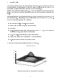
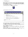
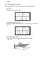
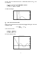
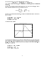
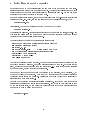
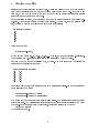
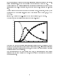
gnuplot 3.5 User's Guide
K C Ang
Division of Mathematics,
NTU-NIE, Singapore.
[email protected]
June 2000
1 Introduction
This document introduces the new user to gnuplot for Windows. It is a brief document to get
the reader started on using gnuplot to produce a variety of graphs. It is not meant to be a
manual since a detailed online help manual comes with the software.
gnuplot is an interactive plotting program. The two main plotting commands are plot and
splot. The other commands sets various parameters and give you options to customise your
plots.
Besides using gnuplot as an interactive software, one also write script les and load the le
from inside gnuplot. Alternatively, one can run the script in batch mode from the DOS prompt.
Some of the things that gnuplot can do include:
Simple plots of built-in or user-dened functions
Scatter plots of bivariate data, with errorbar options
Bar graphs
Three-dimensional Surface plots of functions of the form z = f (x; y) with options for
hidden line removal, view angles and contour lines
Two- and three-dimensional plots of parametric functions
Plots of data directly from tables created by other applications
Re-generate plots on various output les or devices
An example of a plot created in gnuplot is shown in Figure 1.
Bivariate Normal Density
0.2
0.15
0.1
0.05
0
-4
-3
-2
-1
0
x
1
2
3
4
-4
-3
-2
-1
0
1
Figure 1: An example of a plot produced by gnuplot
2
3
2
y
4
2 Starting gnuplot
is available on computers running a variety of operating systems, including IBM-PCs
and compatibles, UNIX, VAX/VMS, DOS and Windows9x. In this document, it is assumed
that the reader uses a PC (running MS Windows95/98). It is also assumed that gnuplot has
been properly installed on the system.
To start gnuplot, one simply double-clicks on the gnuplot icon:
gnuplot
The following gnuplot window should pop up:
The menu bar, tool bar and buttons that appear on the window look like those on any other
Windows-based applications. This is the interactive gnuplot environment.
To exit gnuplot, you can type either exit, quit or simply q. Alternatively, you can exit by
clicking on File-Exit on the menu bar.
Online Help is available by either typing help at the gnuplot command prompt or clicking
the Help menu item.
gnuplot has a feature that allows you to recall previous commands and edit them. On the PC,
the up/down arrow keys are used to get the previous/next commands.
3
3 Basics
3.1 Plotting pre-dened functions
Start exploring gnuplot by typing the following commands at the gnuplot prompt:
1.
plot sin(x)
This command produces a plot of sin x:
1
sin(x)
0.8
0.6
0.4
0.2
0
-0.2
-0.4
-0.6
-0.8
-1
-10
2.
-5
0
5
10
plot [-pi:pi] cos(x**2), sin(2*x)
This command creates a plot of cos x2 and sin 2x on the same graph, with x ranging from
, to :
1
cos(x**2)
sin(2*x)
0.8
0.6
0.4
0.2
0
-0.2
-0.4
-0.6
-0.8
-1
-3
3.
-2
-1
0
1
2
3
splot [-3:3] [-3:3] x**2*y
This command produces a three-dimensional surface plot of the function
f (x; y) = x2 y:
x**2*y
30
20
10
0
-10
-20
-30
-3
-2
-1
0
1
2
4
3
-3
-2
-1
0
1
2
3
In the above three examples, we have used gnuplot's built-in functions sin(), cos() and exp().
We have also used the built-in or pre-dened constant pi. The complete list can be found in
gnuplot's manual.
In the rst example above, the plot command tells gnuplot to produce a two-dimensional plot.
As the range for x is not specied, gnuplot uses its default range of (,10; 10).
In the second example, we specify the range for x (from , to ) by typing [-pi:pi] following
the plot command. The two functions to be plotted are separated by a comma. Note that on
a colour screen, gnuplot uses dierent colours for the functions. On a monochrome display (or
if the output is directed to a non-colour eps le as in the case here), the functions are plotted
using dierent line styles.
In the last example, we set the x and y values to range from -3 to 3. Note that the ranges are
optional in both plot and splot commands.
A sample of gnuplot's pre-dened functions is given below:
gnuplot
abs
acos
asin
atan
cos
cosh
exp
floor
int
log
log10
rand
sgn
sin
sinh
sqrt
tan
tanh
function Description
absolute value
inverse cosine
inverse sine
inverse tangent
cosine
hyperbolic cosine
exponential
largest integer not greater than its argument
integer part of the argument
natural logarithm
common logarithm (i.e. base 10)
pseudo random number
sign function
(1 if argument is positive, -1 if negative, 0 if zero)
sine
hyperbolic sine
square root
tangent
hyperbolic tangent
For a complete list, refer to the online help on gnuplot.
5
3.2 More on Setting Ranges
If you wish to specify the y-range but not the x-range for a plot, put in both sets of brackets
but leave the rst empty. For instance,
plot [] [0:4] 1/(x**3)
The command set has many options and is used to control various components of a plot. In
the previous examples, we saw how we can set the ranges of our plots by specifying them in the
plot or splot commands. The ranges can also be set before plotting using the commands set
xrange, set yrange and set zrange. For instance,
set xrange [-3*pi:3*pi]
set yrange [:20]
set zrange [-exp(2.7):sin(pi/2)]
You may omit either the upper or the lower limits. The limits may be numbers or pre-dened
constants, or expressions.
3.3 Setting Labels and Titles
We may give the axes a label and the plot a title using commands such as the following:
set xlabel 'x'
set ylabel "Host Population"
set title 'Graph of y against x'
replot
Note that both single quote and double quote are acceptable. The
redraws the previous plot, incorporating new settings or changes.
6
replot
command simply
4 User-dened Constants and Functions
4.1 Simple constants and expressions
If we use constants or functions repeatedly, we may wish to dene them using names that we
can remember easily. For this purpose, we will need to know how arithmetic and expressions
are written in gnuplot. The arithmetic and logical expressions used in gnuplot are basically
similar to those used in Fortran or C.
Some common binary operators are listed below:
Symbol
Example
**
*
/
%
+
==
!=
Explanation
exponentiation
multiplication
division
modulo
addition
subtraction
equality
inequality
a**b
a*b
a/b
a%b
a+b
a-b
a==b
a!=b
As an example of a user-dened function with some xed constants, suppose we wish to graph
the function
1 e, x,
f (x) = p
2
where = 9:256 and = 6:395.
The following set of commands may be used:
(
)2
2 2
m=9.256
s=6.395
f(x) = 1/(sqrt(2*pi)*s)*exp(-(x-m)**2/(2*s**2))
plot [-10:50] f(x)
This produces the following graph:
0.07
0.06
0.05
0.04
0.03
0.02
0.01
0
-10
0
10
20
7
30
40
50
Suppose we wish to the dierent plots produced by dierent sets of values of and , we may
do the following:
f(x,m,s) = 1/(sqrt(2*pi)*s)*exp(-(x-m)**2/(2*s**2))
plot [-5:20] f(x,8,3), f(x,3.5,1)
The following is obtained:
0.4
f(x,8,3)
f(x,3.5,1)
0.35
0.3
0.25
0.2
0.15
0.1
0.05
0
-5
0
5
10
15
20
4.2 Piecewise continuous functions
can also plot functions which are piecewise continuous. For instance, if we wish to plot
the following function
,x;
x<0
f (x) =
sin(x); x 0 :
gnuplot
We can use the commands:
f(x)=(x<0) ? -x:sin(x)
plot [-5:] [-2:] f(x)
and obtain the following graph:
A Piecewise Continuous Function
5
f(x)
4
3
2
1
0
-1
-2
-4
-2
0
2
8
4
6
8
10
In the above example, we have used gnuplot's ternary operator:
<condition>
?
<expression1>
<expression2>
:
which means if <condition> is true, then <expression1> is evaluated, otherwise <expression2>
is evaluated.
In order to dene continuous piecewise functions which have more than two pieces, we need to
use the following trick: suppose we have a function dened as
8
< x + 2;
f (x) = x2 + 2x;
: 4 , x;
x < ,2
,2 x < 1 :
x1
In order to dene this function in gnuplot, we string two functions together and then plot the
second function:
f1(x)=(x<-2) ? x+2 : x**2+2*x
f2(x)=(x<1) ? f1(x) : 4-x
plot [-6:] [:4] f2(x)
The following graph results:
Another Piecewise Continuous Function
4
f2(x)
3
2
1
0
-1
-2
-3
-4
-6
-4
-2
0
2
4
6
Note that gnuplot will connect the endpoints with straight lines even if the piecewise function
is not continuous. This is not satisfactory as we may wish to plot discontinuous functions at
times. One way to overcome this is to set the unwanted sections to something unprintable. For
instance, try the following:
f1(x)=(x<0) ? -1 : sqrt(-1)
f2(x)=(x<0) ? x/0 : 1
plot [] [-2:2] f1(x), f2(x)
9
5 Script les and Batch Processing
It is quite common to nd ourselves using the same set of commands over and over again.
le. The le simply consists of the commands
or statements that you would enter interactively at the gnuplot prompt. We can use a text
editor (such as Notepad) to create or edit such a le.
Once such a script le is created, it can be run or processed in two ways. Suppose the script le
is called \mygraph.gp". First, you can run gnuplot and at the gnuplot prompt, type:
gnuplot allows us to put such commands in a script
load "mygraph.gp"
Alternatively, you can run the script le at the DOS prompt by typing:
wgnuplot mygraph.gp
This will invoke gnuplot. After it nishes executing the commands in the script, it exits. Note
that there is a pause command which can be used to pause the execution of the commands in
the script until the user presses the RETURN key.
The script le used to produce the previous plot is given here:
# script for plotting a piecewise continuous function
set terminal postscript eps 14
set size 1.0, 1.0
set output "graph.eps"
# save output to a file
set title "Another Piecewise Continuous Function"
f1(x)=(x<-2) ? x+2 : x**2+2*x
f2(x)=(x<1) ? f1(x) : 4-x
plot [-6:] [:4] f2(x)
Note that the rst line begins with a \#". Anything that comes after this symbol is a comment
and will be ignored by gnuplot. Hence the rst line is simply a comment. Note also that on
line 4, we place a comment after the command \set output ...". This is done to remind ourselves
what we are doing, making the script more readable.
If a command is too long and needs to be continued to the next line, put a backslash, n, at
the end of the line to be continued. Note that the n character must be the last character in
the line (no spaces should come after it). Multiple commands can be placed on a single line by
separating them with a semicolon, ;.
Suppose we have started an interactive session of gnuplot. Suppose we have dened some
variables and functions and customised some settings. If we wish to keep all these so that
we can use it again later, we can write them (along with all of the other default values and
commands) to a le by giving the command:
save 'myfile.gp'
10
6 Plotting Data les
gnuplot can
produce plots from tabulated data. This is very useful when we have data obtained
from another application and we wish to produce a graph for the set of data. Note that in the
data le, we can put comments in the same way as we can in a script le; gnuplot ignores
everything that comes after the # symbol.
In the discussion to follow, we shall assume that our data sets are stored in a le called \values.dat". The le should contain one data point per line. For example, for a one variable data
set, the le may contain the following set of data for that variable:
# a sample data set
2.2
3.5
5.6
8.9
7.4
Using the command:
plot 'values.dat',
we can plot the points (0,2.2), (1,3.5), (2,5.6), ... That is, the data set gives the y-coordinate.
The corresponding x-coordinate starts from 0 and increases by 1 for each value.
Suppose we have a data set consisting of (x; y) pairs. The data set should be organised in
columns as in the following example:
# another sample data set
0.5
2.2
1.2
3.5
1.8
5.6
3.2
8.9
4.9
7.4
Suppose we wish to plot these points and join them using straight lines. We may use either one
of the following commands:
plot 'values.dat' with lines
plot 'values.dat' with linespoints
The option that comes after with is called a plot style. The lines style connects adjacent
points with lines. The linespoints style connects the points as well as displays a symbol at
the points. For more information on plot styles, consult the online help by typing
help plot styles
at the gnuplot prompt.
11
Suppose we have a table of values where only the rst column is the independent variable and
the other columns contain values of some other dependent variables. For instance, one data set
could look like this:
# a table of values
# t
P
Q
0
1.2
2.2
1
2.1
2.9
2
2.9
3.1
3
3.5
3.7
4
4.0
4.5
R
3.8
3.6
2.2
1.1
0.2
To obtain a plot of P , Q and R against t on the same pair of axes, we could, for example, use
the command:
n
plot 'values.dat' title 'P' with linespoints,
'values.dat' using 3 title 'Q' with linespoints,
'values.dat' using 4 title 'R' with linespoints
n
Recall that the backslash represents a continuation to the next line. In the above command, we
have given a title to each plot. These will appear in the key or legend of the plot. The number
following the word using tells gnuplot the column to nd the values to be plotted.
As a further example, consider the following set of data obtained from a simulation of an
epidemic. The values were obtained from a Fortran program, tabulated and saved to a le
called \epi.dat". A portion of the le is shown below:
1
2
3
4
...
...
67
68
69
70
979.510
978.805
977.790
976.331
.......
.......
0.038
0.036
0.035
0.033
1.440
2.073
2.984
4.294
......
......
83.113
78.959
75.013
71.263
20.050
20.122
20.226
20.375
.......
.......
917.849
922.005
925.953
929.703
We could use the following script to create a plot:
set terminal postscript eps 14
set size 1.2, 1.0
set output "epi.eps"
set key 60,500
plot "epi.dat" title 'x(n)' with linespoints, \
"epi.dat" using 3 title 'y(n)' with linespoints, \
"epi.dat" using 4 title 'z(n)' with linespoints
12
In the above script, we rst set the terminal to postscript eps so as to create an eps (encapsulated postscript) le. the number \14" refers to the font size of any text in the le.
The set size command basically tells gnuplot the relative dimensions for the width and height
(respectively) of the plot. In this example, we want the plot to be 1.2 units wide and 1.0 units
high.
The set output command sets the output to the specied device. In this case, we wish to have
the plot saved to a le called \epi.eps" so that we can include it as a gure in, say, a LATEX
document.
set key x, y places the key (i.e. legend) of the plot at position (x; y ) on the plot.
The script produces the following plot (saved in the le \epi.eps"):
1000
900
800
700
600
500
x(n)
y(n)
z(n)
400
300
200
100
0
0
10
20
30
40
50
60
70
There are many other ways of customising plots using the set command. For instance, we may
add text to the plot (annotate the graph) using the set label option. We can also draw arrows
or line segments using the set arrow command. Tick marks on the axes can also be set using
the set xtics command for instance.
For more information on the plot and set commands, as well as using and with options
associated with the plot or splot commands, one can refer to the online help manual that
comes with gnuplot.
13
7 Output of Plots
After creating a plot, we usually wish to be able to obtain a hard copy of it, or perhaps to put
the plot onto another document. This can be done in a variety of ways.
One easy way to create a document containing the plot is to copy it to the clipboard and then
paste it onto a word processing document, like MS WORD, for instance. Suppose we have
created a plot using gnuplot and a window displaying the resulting plot pops up. We can then
right-click anywhere on the plot and a menu will pop up. Select Copy to Clipboard from the
menu items and the plot will be copied. We may now open a new WORD document and paste
the plot there.
If we wish to output the plot to some other graphic les, we can use the set terminal command.
We have already seen how to create an encapsulated postscript (eps) le earlier. The eps le
created may then be included in other documents (for example, in a LATEX source document).
Another way to created a plot to be included in a LATEX document is to actually create the LATEX
code for the plot instead of producing an eps le. This is done by using the setting the terminal
option to latex. Setting the terminal type to latex tells gnuplot that we wish to create a plot
in LATEX's picture environment format. gnuplot will create the necessary plot and then convert
to LATEX's graphics language.
Below is an example of a script le used to produce a LATEX le for the plot:
set terminal latex
set output 'plot.tex'
set title 'An Example of plotting in \LaTeX\ with {\sf gnuplot}'
set xrange [-pi:pi]
plot sin(x) title '$\sin x$', cos(x) title '$\cos x$'
Note that in this script, we have included some LATEX code in the gnuplot commands. For
instance, the titles for the individual plots are written in LATEX's mathematics environment,
hence the pair of $ signs.
Running the above script creates a le called \plot.tex", which contains the LATEX source code
for the plot. This le can be inserted into the main LATEX document. To do so, at the point in
the document where the plot is to appear, we insert the following:
\begin{figure}
\begin{center}
\input{plot.tex}
\end{center}
\caption{An Example of a plot generated with the {\tt latex} terminal type}
\end{figure}
14
The following plot is obtained:
1
0.8
0.6
0.4
0.2
0
-0.2
-0.4
-0.6
-0.8
-1
An Example of plotting in LATEX with gnuplot
sin x
cos x
-3
-2
-1
0
1
2
3
Figure 2: An Example of a plot generated with the latex terminal type
15