Download NS3D v2.14: user's manual

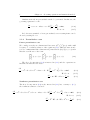
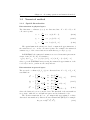
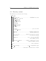
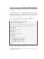
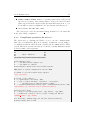
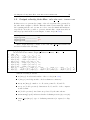
NS3D v2.14: user’s manual
LadHyX - Ecole Polytechnique
Palaiseau - France
Manual v1.01 (10/06/2014)
Author: Axel DELONCLE
[email protected]
Cover illustration: direct numerical simulation of the zigzag instability of a pair of
counter-rotating vertical vortices in a stratified fluid by Deloncle et al. (2008). This simulation, of size 1440 × 1440 × 192, was performed with NS3D on a parallel computer.
Contents
1 Governing equations and numerical method
1.1 Governing equations . . . . . . . . . . . . . . . . . . . .
1.1.1 Non-perturbative case . . . . . . . . . . . . . . .
1.1.2 Perturbative cases . . . . . . . . . . . . . . . . .
1.1.3 Spectral form of the governing equations . . . . .
1.2 Numerical method . . . . . . . . . . . . . . . . . . . . .
1.2.1 Spatial discretisation . . . . . . . . . . . . . . . .
1.2.2 Time discretisation . . . . . . . . . . . . . . . . .
1.2.3 Pseudo-spectral evaluation of the nonlinear term
1.2.4 Dealiasing . . . . . . . . . . . . . . . . . . . . . .
2 Compilation and execution
2.1 Overview . . . . . . . . . . . . . . . . . . . . . .
2.2 Directory content . . . . . . . . . . . . . . . . . .
2.3 Compilation step . . . . . . . . . . . . . . . . . .
2.3.1 Fast Fourier Transform (FFT) libraries .
2.3.2 Preprocessor files config.h and extended
2.3.3 Compilation parameter file Makefile . . .
2.4 Execution step . . . . . . . . . . . . . . . . . . .
2.4.1 Run-time parameter file data.in . . . . .
2.4.2 Running the executable ns3d . . . . . . .
2.5 Test case . . . . . . . . . . . . . . . . . . . . . .
.
.
.
.
.
.
.
.
.
.
.
.
.
.
.
.
.
.
.
.
.
.
.
.
.
.
.
5
5
5
6
7
8
8
9
9
10
. . . . . .
. . . . . .
. . . . . .
. . . . . .
config.h
. . . . . .
. . . . . .
. . . . . .
. . . . . .
. . . . . .
.
.
.
.
.
.
.
.
.
.
.
.
.
.
.
.
.
.
.
.
13
13
14
15
15
16
17
19
19
22
22
.
.
.
.
.
.
.
.
27
27
27
28
28
29
31
31
31
3 Input and output binary files
3.1 General remarks on binary files in FORTRAN . . . . . .
3.1.1 Headers and trailers of records . . . . . . . . . .
3.1.2 Array storage order . . . . . . . . . . . . . . . .
3.1.3 Endian order . . . . . . . . . . . . . . . . . . . .
3.2 Output velocity/state files: velo rho vort.t=xxxx.xxx
3.3 Initial velocity/state: velo type . . . . . . . . . . . . .
3.3.1 Reading velocity.init . . . . . . . . . . . . . .
3.3.2 Internal subroutine . . . . . . . . . . . . . . . . .
.
.
.
.
.
.
.
.
.
.
.
.
.
.
.
.
.
.
.
.
.
.
.
.
.
.
.
.
.
.
.
.
.
2
CONTENTS
3.4
3.3.3 White noise . . . . . .
Base state: base2D type . . .
3.4.1 Reading base2D.init
3.4.2 Internal subroutine . .
.
.
.
.
.
.
.
.
.
.
.
.
.
.
.
.
.
.
.
.
.
.
.
.
4 MPI parallel run
4.1 Running a MPI run: quick start . . . .
4.2 Details of the MPI implementation . . .
4.2.1 Data distribution and transposed
4.2.2 FORTRAN array indexes . . . .
5 Performances
5.1 Memory . . . . . . . . . . . . . . .
5.1.1 Memory usage . . . . . . .
5.1.2 Memory location . . . . . .
5.2 Speed . . . . . . . . . . . . . . . .
5.2.1 Time-consuming steps . . .
5.2.2 FFT libraries performances
5.2.3 MPI speed-up . . . . . . . .
.
.
.
.
.
.
.
.
.
.
.
.
.
.
.
.
.
.
.
.
.
.
.
.
.
.
.
.
.
.
.
.
.
.
.
.
.
.
.
.
.
.
.
.
.
.
.
.
.
.
.
.
.
.
.
.
.
.
.
.
.
.
.
.
.
.
.
.
.
32
32
32
33
. . .
. . .
FFT
. . .
.
.
.
.
.
.
.
.
.
.
.
.
.
.
.
.
.
.
.
.
.
.
.
.
.
.
.
.
.
.
.
.
.
.
.
.
.
.
.
.
35
35
37
37
39
.
.
.
.
.
.
.
43
43
43
44
45
45
45
47
.
.
.
.
.
.
.
.
.
.
.
.
.
.
.
.
.
.
.
.
.
.
.
.
.
.
.
.
.
.
.
.
.
.
.
.
.
.
.
.
.
.
.
.
.
.
.
.
.
.
.
.
.
.
.
.
.
.
.
.
.
.
.
.
.
.
.
.
.
.
.
.
.
.
.
.
.
.
.
.
.
.
.
.
.
.
.
.
6 Frequently asked questions (FAQ)
49
Bibliography
55
Introduction
NS3D is a direct numerical simulation (DNS) code that integrates the incompressible Navier–Stokes Three-Dimensional (NS3D) equations. Its main specifications are:
ˆ pseudo-spectral numerical method, imposing periodic boundary conditions,
ˆ homogeneous fluid, or stratified fluid under the Boussinesq approximation,
ˆ possibility to add a frame background rotation,
ˆ non-perturbative simulations or perturbative simulations around a base
state,
ˆ sequential execution or parallel MPI execution,
ˆ written in FORTRAN 90 for a Unix/Linux environment.
It was first written for a homogeneous fluid by Vincent & Meneguzzi (1991)
and later adapted to stratified fluids by Billant & Chomaz (2000) and Otheguy
et al. (2006). The parallel mode of the code was implemented by Deloncle et al.
(2008).
Chapter 1
Governing equations and
numerical method
1.1
Governing equations
1.1.1
Non-perturbative case
The code integrates the incompressible Navier–Stokes equations within the
Boussinesq approximation in a frame rotating at angular velocity Ωb about the
vertical z-axis:
p
u2
∂u
= u × ω − 2Ωb ez × u − ∇
+ bez + ν∆u,
(1.1a)
+
∂t
ρ0
2
∇ · u = 0,
(1.1b)
ν
∂b
+ u · ∇b + N 2 w =
∆b,
(1.1c)
∂t
Sc
where u = (u, v, w) is the velocity vector in Cartesian coordinates (x, y, z),
ω the vorticity, ρ0 a constant reference density, p the pressure, b = −gρ/ρ0
the buoyancy with ρ the density perturbation with respect to the base density
ρ0 + ρ(z),
p g the gravity and ez the unit vector in the upward z-direction.
N = −g/ρ0 dρ/dz is the Brunt–V¨ais¨al¨a frequency assumed here constant,
ν is the kinematic viscosity and Sc = ν/D the Schmidt number with D the
molecular diffusivity of the stratifying agent.
We consider periodic boundary conditions:
 
 
u
u
 p  (x + Lx , y + Ly , z + Lz , t) =  p  (x, y, z, t),
b
b
where Lx , Ly and Lz are the computational domain sizes.
(1.2)
6
Chapter 1
Governing equations and numerical method
Simulations in a homogenous fluid can also be performed. In this case, the
governing equations become:
∂u
u2
p
+
+ ν∆u,
(1.3a)
= u × ω − 2Ωb ez × u − ∇
∂t
ρ0
2
∇ · u = 0.
(1.3b)
In both cases, stratified or homogenous fluid, a non-rotating frame can be
chosen by setting Ωb = 0.
1.1.2
Perturbative cases
Linear perturbative case
We consider a steady two-dimensional base state (ub , pb , bb )(x, y) with a null
buoyancy bb = 0 that is solution of the equations (1.1). This base state is subjected to infinitesimal three-dimensional perturbations (˜
u, p˜, ˜b)(x, y, z, t) such
that the total flow is of the form:
 
 b
 
˜
u
u
u
 p  (x, y, z, t) =  pb  (x, y) +  p˜ (x, y, z, t).
(1.4)
˜
b
0
b
The flow decomposition (1.4) is inserted in (1.1) and the equations are
linearized around the base state:
∂u
˜
p˜
b
b
b
=u ×ω
˜ +u
˜ × ω − 2Ωb ez × u
˜−∇
+u ·u
˜ + ˜bez + ν∆˜
u,
∂t
ρ0
∇·u
˜ = 0,
˜
∂b
ν ˜
+ ub · ∇˜b + N 2 w
˜=
∆b.
∂t
Sc
(1.5a)
(1.5b)
(1.5c)
Nonlinear perturbative case
The flow decomposition (1.4) is also inserted in (1.1) but, contrary to (1.5),
the nonlinear terms are conserved:
∂u
˜
p˜
u
˜2
= ub × ω
˜ +u
˜ × ωb + u
˜ × ω − 2Ωb ez × u
˜−∇
+ ub · u
˜+
+ ˜bez + ν∆˜
u,
∂t
ρ0
2
∇·u
˜ = 0,
∂˜b
ν ˜
+ ub · ∇˜b + u
˜ · ∇˜b + N 2 w
˜=
∆b.
∂t
Sc
(1.6a)
(1.6b)
(1.6c)
1.1 Governing equations
1.1.3
7
Spectral form of the governing equations
We apply three-dimensional Fourier transforms to the terms of the equations (1.1), for example:
1
u
ˆ(kx , ky , kz , t) =
Lx Ly Lz
Z LZ
Z
x Ly
0
0
Lz
u(x, y, z, t)e−i(kx x+ky y+kz z) dxdydz, (1.7)
0
where the hat denotes the Fourier transform, i the imaginary unit and kx ,
ky and kz are the components of the total wavenumber k = (kx , ky , kz ). In
spectral space, the governing equations (1.1) are replaced by:
∂u
ˆ
\
= P(k) u
× ω − 2Ωb ez × u
ˆ + ˆbez − νk2 u
ˆ,
∂t
∂ˆb
ν 2ˆ
c − N 2w
= −ik · bu
ˆ−
k b.
∂t
Sc
(1.8a)
(1.8b)
The tensor P(k) with Cartesian components Pij = δij − ki kj /k2 designates
the projection operator on the space of solenoidal fields so as to enforce the
incompressibility condition k · u
ˆ = 0. The viscous and diffusive terms are
integrated exactly. This leads to the equations actually integrated in time by
NS3D:
∂u
ˆeνk
∂t
2t
h
i
2
\
= P(k) u
× ω − 2Ωb ez × u
ˆ + ˆbez eνk t ,
ν 2
k t
Sc
∂ˆbe
∂t
h
i ν 2
c − N 2w
= −ik · bu
ˆ e Sc k t .
(1.9a)
(1.9b)
One may note that that the pressure field p does not appear in the spectral
form (1.9) of the governing equations. The pressure field is not solved by NS3D
and should be deduced from (u, b) if necessary.
The generalisation to the perturbative cases is straightforward, and will not
be detailed here.
8
Chapter 1
Governing equations and numerical method
1.2
Numerical method
1.2.1
Spatial discretisation
Discretisation in physical space
The Cartesian coordinates (x, y, z) are discretised into N = Nx × Ny × Nz
collocation points:
Lx
Nx
Ly
= j
Ny
Lz
= k
Nz
xi = i
for i ∈ [0, Nx − 1],
(1.10a)
yj
for j ∈ [0, Ny − 1],
(1.10b)
for k ∈ [0, Nz − 1].
(1.10c)
zk
The spatial numerical schemes are based on numerical approximations of
the variables u, b etc. on the collocation points. For example, the numerical
estimate ui,j,k of the exact solution u is such that ui,j,k ≈ u(xi , yj , zk ).
In FORTRAN, the numerical estimates are stored in double precisionarrays of size [Nx , Ny , Nz ]. For instance:
ux (i, j, k) = ui,j,k
for
(i, j, k) ∈ [0, Nx − 1] × [0, Ny − 1] × [0, Nz − 1],
where ux is the FORTRAN array storing the numerical approximation of the
x-velocity u and i, j and k are the array indexes.
Discretisation in spectral space
The spectral coordinates (kx , ky , kz )
wavenumbers:
(
ik L2πx
ik
kx =
(ik − Nx ) L2πx
(
jk L2πy
kyjk =
(jk − Ny ) L2πy
(
kk L2πz
kk
kz =
(kk − Nz ) L2πz
are discretised into N = Nx × Ny × Nz
for ik ∈ [0, N2x ],
for ik ∈ [ N2x + 1, Nx − 1],
for jk ∈ [0,
for jk ∈ [
Ny
2 ],
Ny
2
+ 1, Ny − 1],
for kk ∈ [0, N2z ],
for kk ∈ [ N2z + 1, Nz − 1],
(1.11a)
(1.11b)
(1.11c)
where the divisions by 2 are rounded down. The first half of the wavenumbers
are positive, while the second half is negative and in backwards order.
The Fourier transforms u
ˆ, ˆb etc. are numerically approximated on these
discretised wavenumbers by Discrete Fourier Transforms (DFT). For example:
u
ˆik ,jk ,kk ≈ u
ˆ(kxik , kyjk , kzkk ),
(1.12)
1.2 Numerical method
9
where u
ˆik ,jk ,kk is the Discrete Fourier Transform of ui,j,k :
u
ˆik ,jk ,kk
y −1 Nz −1
NX
x −1 N
X
X
·j
·i
·k
1
−i2π ik
+ jk
+ kk
Nx
Ny
Nz
ui,j,k e
=
.
Nx Ny Nz
i=0
j=0
(1.13)
k=0
This Discrete Fourier Transform can easily be shown to possess the “Hermitian” symmetry, u
ˆik ,jk ,kk = u
ˆNx −ik ,Ny −jk ,Nz −kk , where the overline denotes
the complex conjugate. As a result of this symmetry, half of the values of
u
ˆik ,jk ,kk is redundant, being the complex conjugate of the other half, and thus
are not stored in NS3D.
In FORTRAN, we have chosen to store only the first half of the kx -modes,
corresponding to positive kx -wavenumbers. More precisely, the Discrete Fourier
Transforms are stored in double precision-arrays of size [2, Nx /2+1, Ny , Nz ].
For instance:
)
ux (1, ik , jk , kk ) = Re(ˆ
^
uik ,jk ,kk )
Nx
for (ik , jk , kk ) ∈ 0,
×[0, Ny −1]×[0, Nz −1],
2
ux (2, ik , jk , kk ) = Im(ˆ
^
uik ,jk ,kk )
where ^
ux is the FORTRAN array storing the Discrete Fourier Transform of
ux (i, j, k) and where Re and Im are the real part and the imaginary part,
respectively.
1.2.2
Time discretisation
The following time schemes can be chosen, with a constant time step δt:
ˆ Adams–Bashforth of order two,
ˆ Runge–Kutta of order two,
ˆ Runge–Kutta of order three,
ˆ Runge–Kutta of order four.
A higher-order time scheme implies more numerous evaluations of the nonlinear terms of (1.9) at each time step, but stability is usually achieved for larger
time steps. More details about these classical time schemes can be found in
textbooks.
1.2.3
Pseudo-spectral evaluation of the nonlinear term
The time schemes require the evaluation of the nonlinear terms in brackets
in (1.9). These terms are computed with a pseudo-spectral method from u
ˆ
and ˆb by performing the following steps:
10
Chapter 1
Governing equations and numerical method
1. we evaluate the vorticity in spectral space ω
ˆ = ik × u
ˆ.
2. we apply backward Fourier transforms to the spectral terms u
ˆ, ω
ˆ and ˆb
to obtain u, ω and b in the physical space.
3. we evaluate the nonlinear terms u × ω and bu in physical space.
4. A forward Fourier transforms is applied to the physical terms u × ω and
c in the spectral space.
\
bu to obtain u
× ω and bu
\
5. we evaluate the nonlinear terms P(k) u
× ω − 2Ωb ez × u
ˆ + ˆbez and
c − N 2w
−ik · bu
ˆ in spectral space.
This algorithm makes an extensive use of Discrete Fourier Transforms at
steps 2 and 4. These Discrete Fourier Transforms are performed with a FastFourier Transform (FFT) algorithm. As detailed in § 5.2.1, the FFTs are the
most time-consuming steps of the algorithm, requiring usually 70–95% of the
total calculation time.
1.2.4
Dealiasing
The Discrete Fourier Transforms of a periodic function introduces the so-called
aliasing error (Gottlieb & Orszag 1977), which is partially due to the artificial
periodicity of the discrete Fourier coefficient as a function of the wavenumber.
The aliasing error pollutes the accuracy of the high-order modes, especially
those last 1/3 of the high-order modes.
To limit aliasing errors, NS3D allows to truncate high-order spectral modes
at each time step of the time scheme. Two dealiasing functions are available.
Squared dealiasing
The following spectral modes are truncated:


|kxik |> rxk kxmax ,

u
ˆik ,jk ,kk
jk
k max
ˆbik ,jk ,kk = 0 if or |ky |> ry ky ,

or |kzkk |> rzk kzmax ,
where kxmax , kymax and kzmax are the maximum positive wavenumbers defined in (1.11) and rxk , ryk , and rzk are the truncation radius, along the three
spectral directions, set by the user. For instance, a value rxk = 0 implies that
all the modes are truncated along the kx -direction while rxk > 1 means that no
mode is truncated.
1.2 Numerical method
11
The classical 2/3-rule by Orszag (1971), that removes most of the aliasing
effects, is equivalent to rxk = ryk = rzk = 2/3. However this implies to truncate
a large number of high-order modes and thus decrease the spectral and spatial
resolution of the simulation. Depending on the nature of the physical problems,
truncating fewer modes may or may not be sufficient.
Elliptic dealiasing
The following spectral modes are truncated:
u
ˆik ,jk ,kk
ˆbik ,jk ,kk = 0
if
kxik
rxk kxmax
2
+
kyjk
ryk kymax
!2
+
kzkk
rzk kzmax
2
> 1.
Chapter 2
Compilation and execution
2.1
Overview
The mains steps to use the NS3D code are the following:
1. Compiling the code:
(a) installing a third-party Fast Fourier Transform (FFT) library,
(b) editing the preprocessor file config.h,
(c) compiling the source files with a Makefile to generate the executable ns3d.
2. Running the code:
(a) editing the run-time parameter file data.in,
(b) (optional) generating an initial velocity/state file velocity.init,
(c) (optional) generating a base state file base2D.init,
(d) running the executable ns3d.
These steps are detailed in the following sections, in the case of a sequential
execution. The specificities of parallel MPI runs are presented in § 4.
14
Chapter 2
2.2
Compilation and execution
Directory content
The NS3D directory structure is the following:
NS3D-2.14/
source/
MPI Times.F90............................FORTRAN source files
timing.F90 .3 fft.F90
data parser.F90
global vars.F90
subfunctions.F90
input.F90
output.F90
gen velocity.F90
time scheme.F90
main.F90
config.h.......................................preprocessor files
extended config.h
Makefile .............................. compilation parameter file
data.in .................................. run-time parameter file
velocity.init.................initial velocity/state file [optional]
base2D.init ............................. base state file [optional]
JMFFT-8.0/ .....................
source of the third-party FFT
library JMFFT [optional]
Makefiles examples/ .........examples of Makefiles for various
compilers and FFT [optional]
doc/ ............................................ this documentation
post processing/ .................... post processing Matlab scripts
jobs/......................bash scripts to automate the use of NS3D
2.3 Compilation step
15
The only files that are mandatory to use NS3D are located in the source
directory. The other files are optional and are only provided in the hope of
helping.
2.3
2.3.1
Compilation step
Fast Fourier Transform (FFT) libraries
As a pseudo-spectral code, NS3D makes an extensive use of FFTs. The FFT is
not embedded in the NS3D source code and must be provided by a third-party
FFT library, installed on the system. To install a library, please refer to the
intructions of the FFT library provider.
The FFT library must be interfaced with NS3D through the interface module fft.F90 that contains the following generic interface subroutines:
ˆ init fft: this subroutine is called once at the beginning of the NS3D
code. It performs all the required initialisation operations before doing
a forward or a backward FFT.
ˆ fwd fft: this subroutine performs a forward three-dimensional Real-toComplex FFT i.e. from physical space to spectral space.
ˆ bck fft: this subroutine performs a backward three-dimensional Complexto-Real FFT i.e. from spectral space to physical space.
Interfacing a new FFT library with NS3D requires only to write the corresponding previous subroutines. No additional modification in the body of the
NS3D code is necessary.
The FFT interface to use, is defined, at the compilation step, through a
preprocessor flag of the Makefile (see § 2.3.3). The following FFT interfaces
are already available in the current version of NS3D:
ˆ JMFFT 8.0 (flag: -DJMFFT): a FFT library, written in FORTRAN by
Jean-Marie Teuler, that emulates most of the Cray-SCILIB library.
ˆ FFTW 3.2 (flag: -DFFTW): the FFTW library developped by Frigo & Johnson (2005) (http://www.fftw.org). Usually the fastest library on scalar
processors (x86, IBM PowerPC).
ˆ ESSL 4.2 (flag: -DESSL): a fast library on IBM PowerPC processors.
Provided by IBM.
ˆ MathKeisan 1.6.0 (flag: -DMATHKEISAN): the fastest library on vectorial
NEC-SX processors. Provided by NEC.
16
Chapter 2
Compilation and execution
ˆ ASL 19.0 (flag: -DASL): an older NEC library designed for NEC-SX processors.
The FORTRAN source code of the JMFFT 8.0 library is included along the
NS3D source code. It allows to compile and run NS3D, without any installed
external FFT library. However, the JMFFT library is usually slower than the
other options, and thus should be avoided if possible. In most situations, the
FFTW library is the preferred choice.
2.3.2
Preprocessor files config.h and extended config.h
The text file config.h must be in the NS3D directory:
! *******************************************
!
NS3D: compilation parameters
! *******************************************
! This file is used by the preprocessor during the compilation step.
! Avoid multiple inclusions of this file. Do not change!
#ifndef CONFIG_H
#define CONFIG_H
! Number of colocation points
#define DIMX 64
#define DIMY 256
#define DIMZ 3
! Padding along each direction
#define PPADKX 0
#define PPADKY 0
#define PPADKZ 0
! The following time schemes are available:
!
- AB2: Adams-Bashforth of order 2
!
- RK2: Runge and Kutta of order 2
!
- RK3: Runge and Kutta of order 3
!
- RK4: Runge and Kutta of order 4
#define RK4
#endif
This file contains preprocessor variables used at the compilation step. The
variables coloured in red must be edited by the user:
ˆ DIMX, DIMY, DIMZ: number of collocation points Nx , Ny and Nz , along
each physical direction,
2.3 Compilation step
17
ˆ PPADKX, PPADKX, PPADKZ: number of padding values along each spectral
direction kx , ky and kz . The padding values correspond to extra non-used
values appended in the arrays storing the main fields such as u, b or ω.
It can improve memory alignment on some systems, and thus speed,
ˆ time-scheme: AB2, RK2, RK3 or RK4.
The other preprocessor file extended config.h must not be modified and
is also used during compilation.
2.3.3
Compilation parameter file Makefile
The easiest way of compiling the NS3D code is to use the command make,
that relies on a Makefile. Here is an example of Makefile corresponding to
a compilation with the GNU Fortran compiler and the JMFFT library. These
options will rarely generate the fastest executable, but this Makefile should
work by default on most systems.
########################################
##
##
##
NS3D - Makefile
##
##
##
########################################
# This Makefile uses :
#
- the GNU Fortran compiler 4.10
#
- the JMFFT 8.0 library
# This Makefile should work on most Linux systems.
#### Start of system configuration section. ####
# command to call the Fortran 90/95 compiler
F90C = gfortran
# options of the compiler:
#
* optimisation: -O3 (Intel, GNU),
#
* real to double automatic conversion : -r8 (Intel),
#
fdefault-real-8 -fdefault-double-8 (GNU),
#
* extended adddressable memory space: -mcmodel=medium (Intel, GNU)
F90C FLAGS = -O3 -fdefault-real-8 -fdefault-double-8
# pre-processor flags:
#
* flag to call the preprocessor: -fpp (Intel), -cpp (GNU)
#
* definition of macros: choice of FFT, testing for NaN etc.
PREPROC FLAGS = -cpp -DJMFFT
# if necessary, linking flags for the Fast Fourier Transform
# (FFT) library that is used
18
Chapter 2
Compilation and execution
FFT LIB =
#### End of system configuration section. ####
FILES = MPI_Times.F90 timing.F90 fft.F90 data_parser.F90 global_vars.F90
subfunctions.F90 input.F90 output.F90 gen_velocity.F90
time_scheme.F90 main.F90
ns3d: extended_config.h config.h $(FILES)
$(F90C) $(F90C_FLAGS) $(PREPROC_FLAGS) $(FILES) -o $@ $(FFT_LIB)
clean:
rm -f *.o *.mod ns3d
The options to edit in this Makefile are the following:
ˆ F90C: command to call the FORTRAN 90/95 compiler. Classical options
are gfortran (GNU), ifort (Intel), xlf90 (IBM XL Fortran), f90 etc.
ˆ F90C FLAG: compiler flags:
– optimizations flags are strongly advised to speed-up the execution of
the code. A classical option, valid on most compilers, is -O3 (GNU,
Intel etc.).
– It is also advised to set a flag enforcing REAL (4-bytes) variables
to be converted into DOUBLE PRECISION (8-bytes) variables.
This is not mandatory as NS3D already only uses DOUBLE PRECISION variables and constants. However, if the source code is
modified without precaution, it can avoid numerical accuracy mistakes. The corresponding flags are, for instance, -fdefault-real-8
-fdefault-double-8 (GNU) or -r8 (Intel).
– For large simulations, it may also be necessary to extend the addressable data memory. The corresponding flag is for instance
-mcmodel=medium (Intel). See § 5.1.2 for more details.
ˆ PREPROC FLAGS: preprocessor flags. The flag to call the preprocessor must
be defined if the preprocessor is not called automatically, for instance
-cpp (GNU) or -fpp (Intel). The FFT library to use (see § 2.3.1) should
also be set here: -DJMFFT, -DFFTW etc.
ˆ FFT LIB: if necessary, the flags to link the third-party FFT library should
be defined here. The JMFFT library is directly compiled from its embedded source code so that no linking is necessary in this example. For
instance, the classical flag to link FFTW library is -lm -lfftw3.
2.4 Execution step
19
To compile the code, set the prompt into the NS3D source directory. The
Makefile, the FORTRAN source files .F90 and the preprocessor files config.h
and extended config.h must be located in the compilation folder. Type the
following command line to automatically generate the executable ns3d:
> make
This executable ns3d is specific to the parameters defined in config.h and
the Makefile, in particular the dimensions Nx × Ny × Nz of the simulation and
the FFT library to use. To avoid any incoherence, it is advised to generate a
new executable ns3d for each new simulation.
2.4
2.4.1
Execution step
Run-time parameter file data.in
The run-time parameter file, data.in, must be located in the same directory
than the executable ns3d and is read at the beginning of each run.
Here is an example of data.in:
********************************************
*
NS3D: simulation parameters
*
********************************************
This file is read at every simulation start.
*** discretisation variables ***
lx___________________________ 200.
ly___________________________ 60.
lz___________________________ 12.5664
dt___________________________ 0.5
begin________________________ 0.
itmax________________________ 2000
de_aliasing__________________ T
squared:1_or_elliptic:2__ 1
radius_truncation_x______ 0.66
radius_truncation_y______ 0.66
radius_truncation_z______ 1.E30
*** physical variables ***
viscosity____________________
stratified___________________
brunt_vaisala_frequency__
schmidt_number___________
2omega_______________________
5.E-7
F
10.
1.
0.
20
Chapter 2
Compilation and execution
*** Type of simulation ***
perturbative_________________ T
linear___________________ T
*** Base state (only perturbative run) ***
base2D_type__________________ tanh
*** Initial velocity ***
velo_type____________________ null
white_noise__________________ 1E-10
*** Output ***
output1_period_______________ 400
output2_period_______________ 1000
output3_period_______________ 0
ˆ lx, ly and lz are the dimensions Lx , Ly and Lz of the computational
domain along each physical direction.
ˆ dt is the fixed time step δt used by the time scheme.
ˆ begin is the arbitrary numerical value of initial time t0 of the simulation.
ˆ itmax is the number of time steps. Consequently, the initial time is begin
and the ending time is begin+itmax×dt.
ˆ de aliasing indicates whether dealiasing (see § 1.2.4) is applied (T) or
not (F). If dealiasing is applied, it is possible to choose between a squared
(1) or elliptic (2) dealiasing. radius truncation x, y, z, are the dealiasing radius rxk , ryk and rzk along each spectral direction.
ˆ viscosity is the viscosity ν of the fluid.
ˆ stratified indicates whether the simulation is in a stratified fluid (T)
or in a homogeneous fluid (F). In a stratified fluid, the Brunt–V¨ais¨al¨a
frequency N and the Schmidt number Sc must be defined.
ˆ 2omega is 2Ωb , twice the angular velocity of the rotating frame. The
non-rotating case corresponds to a value Ωb = 0.
ˆ perturbative indicates whether the simulation is non-perturbative (F)
or perturbative (T). In perturbative mode, the simulation can be linear
perturbative (linear=T) or nonlinear perturbative (linear=F). See § 1.1
for the meaning of the different options.
ˆ base2D type is only used for perturbative simulations. It defines the
two-dimensional base flow:
2.4 Execution step
21
– null: the base flow is null (ub , wb )(xi , yj ) = 0,
– file: the base flow is read from a binary file base2D.init,
– tanh : the base flow is internally generated and has a hyperbolic
tangent profile,
– etc.
See § 3.4 for more details on the available options.
ˆ velo type allows to select the type of initial velocity/state:
– null: the initial velocity/state flow is null (u, b)(xi , yj , zk ) = 0,
– file: the initial velocity/state flow is read from a binary file velocity.init,
– file vortices : the initial velocity/state flow is internally generated and is made of vertical vortices,
– etc.
See § 3.3 for more details on the available options.
ˆ white noise defines whether white noise is added to the initial velocity
flow. It corresponds to the amplitude of the added white noise. A value
white noise=0 corresponds to no noise. See § 3.3 for more details.
ˆ Output defines the number of time-steps between two successive calls of
the different output subroutines. It is generally advised not to call output
subroutines at every time-step as they require computational time. A
value of 0 means that the corresponding subroutine is never called. In
the current code version, three output subroutines are available:
– output1: this subroutine outputs on the terminal screen basic information: elapsed and remaining time, mean quadratic velocity and
velocity growthrate,
– output2: this subroutine writes a velocity/state output binary file
on the disk (see § 3.3),
– output3: this subroutine is empty and can be completed by the
user directly in the source code output.F90.
When, the base flow or the initial velocity/state file are internally generated
by subroutines, additional run-time parameters can be read from data.in. We
present below an example of extra parameters found at the end of a data.in
file. The meaning of these parameters will not be explained here, as they are
specific to user-defined subroutines that are not part of the body of NS3D.
They are not required for a standard simulation.
22
Chapter 2
Compilation and execution
*** additional variables... ***
* Stuart vortices *
concentration_stuart_________ 0.25
* File gaussian vortices *
file_nb_vortices_____________
Vortex 1
position_x_______________
position_y_______________
circulation______________
core_radius______________
Vortex 2
position_x_______________
position_y_______________
circulation______________
core_radius______________
* Random gaussian vortices *
rnd_nb_vortices______________
rnd_min_distance_____________
rnd_mean_gamma_______________
rnd_std_gamma________________
rnd_mean_radius______________
rnd_std_radius_______________
2.4.2
2
3.1415927
3.8165927
2.
0.2
3.1415927
2.4665927
2.
0.2
10
1.
6.28
0.
1.
0.
Running the executable ns3d
The files data.in and, if necessary, velocity.init and base2D.init must be
present in the same folder than the executable ns3d. To run the executable,
type the following command line. The code will execute.
> .\ns3d
2.5
Test case
The parameter files config.h and data.in presented above in §§ 2.3.2 and 2.4.1
correspond to the linear stability study of a horizontal flow sheared horizontally,
the hyperbolic tangent velocity profile, in a homogeneous quasi-inviscid fluid:
Ly
b
b
ex ,
(2.1)
u (y) = u (y) ex = tanh y −
2
For the interested readers, a more complete study of the stability of this
flow can be found in Michalke (1964) and Deloncle et al. (2007).
2.5 Test case
23
This test case is a convenient way to quickly check whether the code was
correctly compiled and run, by studying the growth rate of the most unstable
mode. We present below the screen-output of this simulation: the growth rate
converges towards σ ≈ 0.189. The total simulation time was about 100 seconds
on an Intel Xeon@ 2.13GHz processor.
###################################################
PROGRAM NS3D version 2.14
###################################################
------------------------------------------------------------------------------INITIALIZATION
---------------------------------------------------------------------------------------------------------DIMENSIONS OF THE SIMULATION
64 x
256 x
3
------------------------------------------------------DISCRETIZATION VARIABLES
---------------------------lx..........................
200.00
ly..........................
60.000
lz..........................
12.566
dt..........................
0.50000
begin.......................
0.0000
itmax.......................
2000
de_aliasing.................
T
squared:1_/_elliptic:2...
1
radius_truncation_x......
0.66000
radius_truncation_y......
0.66000
radius_truncation_z......
2.0000
---------------------------PHYSICAL VARIABLES
---------------------------viscosity...................
stratification..............
brunt_vaisala_frequency..
schmidt_number...........
omega2......................
0.50000E-06
F
10.000
1.0000
0.0000
---------------------------TYPE OF RUN
---------------------------perturbative................
linear..................
T
T
---------------------------BASE STATE
---------------------------base2D_type.................
tanh
24
Chapter 2
---------------------------INITIAL VELOCITY
---------------------------velo_type...................
white_noise.................
null
0.10000E-09
---------------------------OUTPUT
---------------------------output1_period..............
output2_period..............
output3_period..............
400
1000
0
Compilation and execution
Initialization of the Fast Fourier Transformation (FFT)
-> JMFFT-8.0 3D (Author: Jean-Marie Teuler, CNRS)
Base state
-> tanh
Initial velocity
-> null
-> white noise
------------------------------------------------------------------------------TIME STEPPING: Runge and Kutta of order 4
------------------------------------------------------------------------------it =
400
time =
200.000
cpu time in sec (elapsed/remaining) =
mean quadratic velocity =
108398573.85692854
growthrate =
0.0000000000000000
0
it =
800
time =
400.000
cpu time in sec (elapsed/remaining) =
19
mean quadratic velocity =
7.2431437148986121E+040
growthrate = 0.18895533389024657
it =
1200
time =
600.000
cpu time in sec (elapsed/remaining) =
39
mean quadratic velocity =
5.6960132779538870E+073
growthrate = 0.18936254811773309
it =
1600
time =
800.000
cpu time in sec (elapsed/remaining) =
59
mean quadratic velocity =
4.7565205774962807E+106
growthrate = 0.18951264498358636
it =
2000
time =
1000.000
cpu time in sec (elapsed/remaining) =
78
mean quadratic velocity =
4.0724780826732005E+139
growthrate = 0.18957510829664204
0
59
39
19
0
2.5 Test case
25
------------------------------------------------------------------------------END OF THE SIMULATION
------------------------------------------------------------------------------------------------------------------------------------------------------------TIMING REPORT: TREE (in sec)
name
#calls
cpu
elapsed
%cpu
%elapsed
------------------------------------------------------------------------------main
1
98.93
99.06
100.0
100.0
------------------------------------------------------------------------------initialization
1
0.03
0.03
0.0
0.0
time_stepping
2000
98.89
99.02
100.0
100.0
time_scheme
2000
97.86
98.02
99.0
99.0
nonlin_term
8000
91.06
91.14
93.0
93.0
curl
8000
1.97
2.01
2.2
2.2
fft
72000
83.20
83.31
91.4
91.4
vect_prod
8000
3.44
3.43
3.8
3.8
projection
8000
2.40
2.36
2.6
2.6
#others
0.06
0.03
0.1
0.0
#others
6.81
6.88
7.0
7.0
projection
2000
0.60
0.59
0.6
0.6
de_aliasing
2000
0.39
0.38
0.4
0.4
output1
5
0.00
0.00
0.0
0.0
output2
2
0.02
0.02
0.0
0.0
#others
0.01
0.00
0.0
0.0
#others
0.01
0.01
0.0
0.0
------------------------------------------------------------------------------------------------------------------------------------------------------------TIMING REPORT: FLAT (in sec)
Time spent in the subroutine but NOT in the nested subroutines
------------------------------------------------------------------------------name
#calls
cpu
elapsed
%cpu
%elapsed
------------------------------------------------------------------------------fft
72000
83.20
83.31
84.1
84.1
time_scheme
2000
6.81
6.88
6.9
6.9
vect_prod
8000
3.44
3.43
3.5
3.5
projection
10000
3.00
2.96
3.0
3.0
curl
8000
1.97
2.01
2.0
2.0
time_stepping
2000
1.03
1.00
1.0
1.0
de_aliasing
2000
0.39
0.38
0.4
0.4
nonlin_term
8000
0.06
0.03
0.1
0.0
initialization
1
0.03
0.03
0.0
0.0
output2
2
0.02
0.02
0.0
0.0
**main
1
0.01
0.01
0.0
0.0
output1
5
0.00
0.00
0.0
0.0
-------------------------------------------------------------------------------
Chapter 3
Input and output binary files
In this chapter, we present the format of the binary files used in NS3D:
ˆ output velocity/state files velo rho vort.t=xxxx.xxx,
ˆ initial velocity/state files velocity.init,
ˆ base state files base2D.init.
3.1
3.1.1
General remarks on binary files in FORTRAN
Headers and trailers of records
The different binary files used in NS3D are opened with the OPEN command
with the attribute FORM=’unformatted’. In FORTRAN, each time the WRITE
statement is issued, a ”record” is written, the record consists in an integer
header, followed by the data, and finally a trailer that matches the header.
The integer header and trailer consist in the number of bytes that are written
in the data section.
So for example the source code:
OPEN(60, FILE=filename, FORM=’unformatted’)
WRITE(60) nx, ny, nz
WRITE(60) nx, ny
CLOSE(60)
writes the following binary file:
12 nx ny nz 12
8 nx ny 8
28
Chapter 3
Input and output binary files
where nx, ny, nz are 4-byte-long integers. Note the extra integers 12 and 8
corresponding to the number of bytes of each record.
When reading a binary file, FORTRAN is also expecting to find similar
headers and trailers for each record. It is necessary to take it into account when
exchanging binary date file between NS3D and other tools (Scilab, Matlab. . . ).
The additional headers and trailers are integers and so are usually coded on
4 bytes; more rarely they can be coded on 8 bytes on some specific 64-bits
systems.
3.1.2
Array storage order
The multi-dimensional arrays that are used throughout NS3D (velocity, buoyancy, vorticity fields. . . ) are stored in column major order by FORTRAN,
meaning that the first array index varies most rapidly. This is also how an
array is dumped to or read from a file.
Let us consider for example a two-dimensional array u(xi , yj ) defined on a
Cartesian grid (x0 , . . . , xn−1 ) × (y0 , . . . , yp−1 ). NS3S writes and reads this velocity field in the following order:
u(x0 , y0 ), u(x1 , y0 ), . . . , u(xn−1 , y0 ), u(x0 , y1 ), u(x1 , y1 ), . . . , u(xn−1 , y1 ), . . . , u(xn−1 , yp−1 )
The generalisation to the three-dimensional arrays used throughout NS3D
is straightforward.
3.1.3
Endian order
Endianness is the attribute of a system that indicates whether numbers are
represented from left to right or right to left. Endianness comes in two varieties,
big-endian and little-endian, and depends on the system processor. PC (Intel,
AMD) are little-endian whereas most of the other processors (PowerPC, NEC,
SGI) are all big-endian.
An endianness difference can cause problems if a computer unknowingly tries
to read binary data written in the opposite format from a file. It can happen
if you create a data file with NS3D on a computer and try to use it as an
input file on another system, not sharing the same endianness. When working
with systems with different endianness, we advise to force all the compilers to
work with a similar endianness. For instance, big-endianness can be enforced
with the flag -convert big endian (Intel) or -fconvert=big-endian (GNU
Fortran) in the Makefile at the compilation step.
3.2 Output velocity/state files: velo rho vort.t=xxxx.xxx
3.2
29
Output velocity/state files: velo rho vort.t=xxxx.xxx
In this section, we present the format of the velocity/state files generated by
the subroutine output2 of NS3D. This subroutine is automatically called at
the beginning and the end of a run, in order to save the initial and final state,
respectively. It is also possible to generate intermediate output state files at
time-steps specified in the section Output of data.in (see § 2.4.1):
*** Output ***
output1_period_______________ 400
output2_period_______________ 1000
output3_period_______________ 0
These output files have a name of the form velo rho vort.t=xxxx.xxx
and their format is the following:
h1 ,
h2 ,
h3 ,
h3 ,
h3 ,
h3 ,
h3 ,
h3 ,
h3 ,
h4 ,
h4 ,
1, Nx , Ny , Nz , Lx , Ly , Lz , dt, dealiasing, trunc type, rtrunc x, rtrunc y, rtrunc z,
nu, stratified, xns, schmidt, omega2, perturbative, linear, h1 \\
time, h2
ux (x0 , y0 , z0 ), . . . , ux (xNx −1 , yNy −1 , zNz −1 ), h3
uy (x0 , y0 , z0 ), . . . , uy (xNx −1 , yNy −1 , zNz −1 ), h3
uz (x0 , y0 , z0 ), . . . , uz (xNx −1 , yNy −1 , zNz −1 ), h3
b(x0 , y0 , z0 ), . . . , b(xNx −1 , yNy −1 , zNz −1 ), h3
wx (x0 , y0 , z0 ), . . . , wx (xNx −1 , yNy −1 , zNz −1 ), h3
wy (x0 , y0 , z0 ), . . . , wy (xNx −1 , yNy −1 , zNz −1 ), h3
wz (x0 , y0 , z0 ), . . . , wz (xNx −1 , yNy −1 , zNz −1 ), h3
ubx (x0 , y0 ), . . . , ubx (xNx −1 , yNy −1 ), uby (x0 , y0 ), . . . , uby (xNx −1 , yNy −1 ), ubz (x0 , y0 ), . . . , ubz (xNx −1 , yNy −1 ),
wbx (x0 , y0 ), . . . , wbx (xNx −1 , yNy −1 ), wby (x0 , y0 ), . . . , wby (xNx −1 , yNy −1 ), wbz (x0 , y0 ), . . . , wbz (xNx −1 , yNy −1 ),
with the following notations:
ˆ hi [integer]: headers and trailers of the records (see § 3.1.1).
ˆ 1 [integer]: fixed flag useful to check endianness consistency.
ˆ Nx , Ny , Nz [integer]: number of collocation points Nx , Ny and Nz .
ˆ Lx , Ly , Lz [double precision]: dimensions Lx , Ly and Lz of the computational domain.
ˆ dt [double precision]: fixed time step δt used by the time scheme.
ˆ dealiasing [logical]: indicates whether dealiasing is active (T) or not (F).
ˆ trunc type [integer]: type of dealiasing truncation (1: squared, 2: elliptic).
h4
h4
30
Chapter 3
Input and output binary files
ˆ rtrunc x, rtrunc y, rtrunc z [double precision]: radius of truncation
rxk , ryk and rzk along each spectral direction.
ˆ nu [double precision]: viscosity ν of the fluid.
ˆ stratified [logical]: indicates whether the simulation is in a stratified
fluid (T) or a homogeneous fluid (F).
ˆ xns [double precision]: Brunt-V¨
ais¨al¨a frequency N .
ˆ schmidt [double precision]: Schmidt number Sc.
ˆ omega2 [double precision]: 2Ωb , twice the rotational speed of the frame.
ˆ perturbative [logical]: non-perturbative (F) or perturbative (T) simulation.
ˆ linear [logical]: for a perturbative run, indicates whether the simulation
is linear (T) or nonlinear (F).
ˆ time [double precision]: time t of the record.
ˆ (ux , uy , uz )(xi , yj , zk ) [double precision]: velocity values u(xi , yj , zk ) on
the collocation points.
ˆ b(xi , yj , zk ) [double precision]: buoyancy values b(xi , yj , zk ) on the collocation points.
ˆ (wx , wy , wz )(xi , yj , zk ) [double precision]: vorticity values ω(xi , yj , zk ) on
the collocation points.
ˆ (ubx , uby , ubz )(xi , yj ) [double precision]: velocity base state ub (xi , yj ) on the
collocation points.
ˆ (wbx , wby , wbz )(xi , yj ) [double precision]: vorticity base state ω b (xi , yj ) on
the collocation points.
Almost all the simulation parameters are enclosed in the output file, along
the main fields (u, b, w)(xi , yj , zk ). This ensures the traceability of the results
and ease post-processing.
The format of the output velocity/state file is identical to the one of the
initial velocity/state file. Thus, it is possible to use an output state file as an
initial state file, in order to resume a simulation (see § 3.3).
3.3 Initial velocity/state: velo type
3.3
31
Initial velocity/state: velo type
A simulation can be initialized with a three-dimensional state flow (u, b)(xi , yj , zk , t0 ),
either read from a file, or internally generated by a subroutine. Moreover, an
additional white noise can be added to the initial state.
3.3.1
Reading velocity.init
The initial state flow can be read from an external file. To select this option,
velo type in data.in must be set to file. The data describing the initial
state flow must be stored in a binary data file called velocity.init. This file
is read once at the beginning of the simulation and must be copied in the same
directory than the executable ns3d.
The initial velocity file has the same expected format than the one of the
output velocity files (see § 3.2), so that an output state file can be used as an
initial state file. However, only part of the data stored in a velocity file is
actually used to initialize a run:
ˆ (ux , uy , uz , b)(xi , yj , zk ) and time are read from the initial velocity file
and are used to initialize the new run,
ˆ Nx , Ny , Nz , Lx , Ly , Lz read in the initial velocity file must match the values
defined in config.h and data.in of the new run,
ˆ all the other physical parameters dt, nu, perturbative etc. are not read
in the initial velocity file. They are freely defined in data.in of the new
run.
ˆ (wx , wy , wz )(xi , yj , zk ) is not read in the initial velocity file, as the vorticity
is re-computed at each time-step,
ˆ (ubx , uby , ubz )(xi , yj ) and (wbx , wby , wbz )(xi , yj ) are not read in the initial velocity file. In perturbative mode, the base flow must be defined independently for the new run (see § 3.4).
3.3.2
Internal subroutine
The other way of defining an initial state flow (u, b)(xi , yj , zk , t0 ) is to use an
internal subroutine within the NS3D code. To select this option, velo type
in data.in file must be set to the name of this internal subroutine, for instance null (null field), tanh or stuart. This internal subroutine is called
at the beginning of the run from the subroutine gen velo which is in the file
gen velocity.F90. It is possible to directly modify the source code of this
subroutine to satisfy his needs.
32
Chapter 3
3.3.3
Input and output binary files
White noise
Finally, it is possible to add white noise to the initial state flow with the variable white noise in data.in. The noise is added to the initial velocity field
u(xi , yj , zk , t0 ). The added noise follows a uniform distribution with a zeromean value. The value defined in white noise corresponds to the maximum
amplitude of the noise. A value white noise=0 means that no noise is added.
This white noise function is especially useful to initialize perturbative simulations, when looking for the most unstable mode. In this case, velo type is
set to null and white noise is added.
3.4
Base state: base2D type
In perturbative mode, the flow is simulated around a steady two-dimensional
base state with a null buoyancy. To avoid any numerical approximation, the
base state vorticity wb must be explicitly provided by the user, and is not
computed from the velocity ub .
The base state to be defined by the user is thus of the form: (ub , wb )(xi , yj ).
This base state can be initialized either by reading a base flow file, or with
an internal subroutine.
3.4.1
Reading base2D.init
The base flow can be read from an external file. To select this option, base2D type
in data.in must be set to file. The data describing the base state flow must
be stored in a binary data file called base2D.init. This file is read once at
the beginning of the simulation and must be copied in the same directory than
the executable ns3d.
The exact format of this base state file is:
h1 ,
h2 ,
h2 ,
1, Nx , Ny , Lx , Ly , h1
ubx (x0 , y0 ), . . . , ubx (xNx −1 , yNy −1 ), uby (x0 , y0 ), . . . , uby (xNx −1 , uNy −1 ), ubz (x0 , y0 ), . . . , ubz (xNx −1 , yNy −1 ),
wbx (x0 , y0 ), . . . , wbx (xNx −1 , yNy −1 ), wby (x0 , y0 ), . . . , wby (xNx −1 , yNy −1 ), wbz (x0 , y0 ), . . . , wbz (xNx −1 , yNy −1 ),
with the following notations:
ˆ hi [integer]: headers and trailers of the records (see § 3.1.1).
ˆ 1 [integer]: fixed flag useful to check endianness consistency.
ˆ Nx , Ny [integer]: number of collocation points Nx and Ny .
h2
h2
3.4 Base state: base2D type
33
ˆ Lx , Ly [double precision]: dimensions Lx and Ly of the computational
domain.
ˆ (ubx , uby , ubz )(xi , yj ) [double precision]: velocity base state ub (xi , yj ) on the
collocation points.
ˆ (wbx , wby , wbz )(xi , yj ) [double precision]: vorticity base state ω b (xi , yj ) on
the collocation points.
3.4.2
Internal subroutine
The other way of defining a base flow (ub , wb )(xi , yj ) is to use an internal subroutine within the NS3D code. To select this option, base2D type
in data.in file must be set to the name of this internal subroutine, for instance file vortices or stuart. This internal subroutine is called at the
beginning of the run from the subroutine gen base2d which is in the file
gen velocity.F90. It is possible to directly modify the source code of this
subroutine to satisfy his needs.
Chapter 4
MPI parallel run
When running large simulations requiring much memory or calculation time,
a parallel run performed on several processes may become necessary. Parallelism, achieved through the use of Message Passing Interface MPI, has been
implemented in NS3D.
4.1
Running a MPI run: quick start
Let us consider a simulation of dimension N = Nx × Ny × Nz to run on p MPI
processes. The procedure is identical to the one of a sequential run described
in § 2.1, except the following changes:
ˆ step 1b: Ny and Nz are not necessary equal but must be both multiple
of the number of processes p. This condition is mandatory,
ˆ step 1c:
– the number of MPI processes must be defined in the Makefile with
the flag -DMPI=p,
– the MPI version of a FFT library must be set in the Makefile. Most
of the FFT interfaces available in the current version of NS3D, have
their MPI counterpart: -DJMFFT MPI, -DFFTW MPI, -DESSL MPI and
-DMATHKEISAN MPI.
Note that the parallelisation of the three-dimensional FFT is implemented directly by NS3D and relies only on sequential one-dimensional
FFTs performed by the third-party library. It means that it is not
required to install a “MPI parallel FFT library” but only the default
sequential one.
36
Chapter 4
MPI parallel run
– the compilation options required by your system MPI library must
be set, for instance -lmpi. Please refer to the documentation of
your system MPI library.
ˆ step 2d: the executable ns3d must be started with the correct shell instructions, as required by your system MPI library, for instance:
> mpirun −np 16 nsd3
where p = 16 is the number of MPI processes. Please refer to your system
MPI library documentation for more details.
It must be noted that the formats of the different input velocity.init,
base2D.init and output velo rho vort.t=xxxx.xxx files are identical between a sequential and a MPI run. This implies that the same input file can be
used either for a sequential or a MPI run. Similarly, the same post-processing
tools can be used with the output files.
We present below an example of Makefile configured at step 1c to perform
a MPI run with p = 16 processes with the FFTW MPI library:
########################################
##
##
##
NS3D - Makefile
##
##
##
########################################
# This Makefile corresponds to a computer using Intel
# FORTRAN compiler 10 and the FFTW library
# MPI parallel mode
#### Start of system configuration section. ####
# command and arguments of the FORTRAN 90/95 compiler
F90C = ifort
F90C_FLAGS = -r8 -O3
# flags to call the preprocessor and definition of
# a preprocessor macros to set the FFT library.
PREPROC_FLAGS = -fpp -DMPI=16 -DFFTW MPI
# if necessary, linking flags for the Fast Fourier Transform
# (FFT) library that is used
FFT_LIB = -lfftw3 -lm -lmpi
#### End of system configuration section. ####
4.2 Details of the MPI implementation
37
FILES = MPI_Times.F90 timing.F90 fft.F90 data_parser.F90 global_vars.F90
subfunctions.F90 input.F90 output.F90 gen_velocity.F90
time_scheme.F90 main.F90
ns3d: extended_config.h config.h $(FILES)
$(F90C) $(F90C_FLAGS) $(PREPROC_FLAGS) $(FILES) -o $@ $(FFT_LIB)
clean:
rm -f *.o *.mod ns3d
4.2
4.2.1
Details of the MPI implementation
Data distribution and transposed FFT
The most important concept to understand in using MPI is the data distribution. In MPI there is no concept of global address space and each process has
its own memory as shown in figure 4.1.
cpu 1
cpu 2
cpu 3
cpu 4
memory
1
memory
2
memory
3
memory
4
memory bus
Figure 4.1: A distributed memory architecture: each process has its own memory.
In MPI, the data structure is split up and resides as “slices” in the local
memory of each task. All the tasks work concurrently and exchange data
through communications by sending and receiving “messages” as illustrated in
figure 4.2. Compared to a global address space, the implementation is more
complex because we have to define explicitly the distribution of the whole data
among the processes as well as each data communication.
We outline here the implementation of the MPI parallelisation of the NS3D
code for a simulation of total size N = Nx × Ny × Nz . In the following, we
denote Nxk = Nx /2 + 1, Nyk = Ny and Nzk = Nz the total number of spectral
modes that are effectively stored in NS3D. We recall that only half of the
kx -modes are stored (see § 1.2.1).
38
Chapter 4
Communication A
MPI parallel run
Communication B
Processor 1
Processor 2
Processor 3
Processor 4
Figure 4.2: The Message Passing Interface (MPI) paradigm: all the tasks run
concurrently and exchange data through different types of communications.
If we consider a simulation running on a computer with p processes, the
data in physical space are stored in the “natural” order (x, y, z∗) where the star
indicates that the z-direction is distributed among the p processes. It means
that each process has a data slice of size Nx × Ny × Nz /p.
We recall here that FORTRAN stores data in column-major order meaning
that contiguous elements in memory correspond to the first dimension of an
array. Accessing array elements that are contiguous in memory is much faster
than accessing elements which are not, due to caching. This is important when
implementing the FFT algorithm in parallel.
We describe below briefly the main steps of a forward three-dimensional
Real-to-Complex FFT:
1. Each process performs a sequence of Ny × Nz /p one-dimensional Realto-Complex FFTs of size Nx along the local x-direction. At this step,
the array ends in the order (kx , y, z∗) with kx indicating that the first
dimension has been switched into spectral space. The data in the kx direction are stored contiguously ensuring a fast memory access for the
one-dimensional FFT.
2. Each process transposes the data between the first and second local dimensions: (kx , y, z∗) → (y, kx , z∗).
3. Each process performs a sequence of Nxk ×Nz /p one-dimensional Complexto-Complex FFTs of size Ny along the local y-direction. Thanks to the
transpose of the previous step, the array is in the order (ky , kx , z∗) ensuring again a fast memory access.
4. We perform a distributed transpose of the data between the processes.
This is done through a MPI communication of type “MPI alltoall” that
distributes the data along the ky -direction in the order (z, kx , ky ∗) i.e.
each process has a data slice of size Nz × Nxk × Nyk /p. This distributed
transpose between directions ky and z is illustrated schematically on figure 4.3.
4.2 Details of the MPI implementation
39
5. Each process performs a sequence of Nxk ×Nyk /p one-dimensional Complexto-Complex FFTs of size Nz along the local z-direction. At this step, the
array is in the order (kz , kx , ky ∗) ensuring again a fast memory access.
This parallel transposed FFT algorithm gives the Discrete Fourier Transform of the original data but transposed from (x, y, z∗) directions into (kz , kx , ky ∗).
An extra distributed transpose has not been implemented, to retrieve the original order, because this would have required time–costly extra communications.
All the other steps of the pseudo-spectral algorithm are simply performed point
by point in both physical space and spectral space and make use only of the
local data of each process. These portions are easy to implement and will not
be detailed further here. The communications between the processes are thus
limited to the distributed transpose performed in the FFT. This makes the distributed memory parallelisation well adapted to the pseudo-spectral algorithm.
It must be noted that, because of the transposed parallel FFT, both Ny
and Nz must be multiple of p. Indeed, Ny = Nyk is splitted between the p
processes in spectral space (kz , kx , ky ∗) while Nz is splitted in physical space
(x, y, z∗).
We finally outline here that this transposed FFT algorithm is directly implemented within the NS3D code and only makes use of sequential one-dimensional
FFTs provided by third-party FFT libraries. We do not rely on MPI threedimensional FFT that may be already available in some FFT libraries. We do
not use, for instance, the MPI version of the library FFTW that is available in
FFTW v3.3 and above.
4.2.2
FORTRAN array indexes
As outlined in § 4.2.1, in MPI parallel mode, NS3D uses a parallel transposed
FFT algorithm giving the Discrete Fourier Transform of the original data but
transposed from (x, y, z∗) directions into (kz , kx , ky ∗). It it not the case for a sequential run where the original order is preserved in spectral space: (kx , ky , kz ).
As a consequence, it means that the spectral directions kx , ky and kz are associated with different FORTRAN array indexes, in sequential and MPI run.
To deal with both situations, the source code makes use of two different sets
of array indexes:
1. ik1, ik2, ik3 corresponds to the FORTRAN storage order, ik1 and ik3
being the inner and outer dimension of the array, respectively. This is
verified in both sequential and MPI run.
40
Chapter 4
MPI parallel run
Distributed transpose
y
contiguous elements
contiguous elements
z
Proc 1
Proc 2
Proc 3
z*
Proc 1
Proc 2
Proc 3
y*
Figure 4.3: Schematic of a distributed transpose with p = 3 processes on a
two-dimensional array of total size Nyk × Nz = 9 × 6. The array is initially
in the order (ky , z∗): the data are distributed along the z-direction and the
ky -direction corresponds to contiguous elements in memory. The distributed
transpose ends up with an array in the order (z, ky ∗): the data are distributed
along the ky -direction and the z-direction corresponds to contiguous elements
in memory.
4.2 Details of the MPI implementation
41
2. IKX, IKY, IKZ corresponds to the spectral directions kx , ky and kz , respectively. During the compilation step, these variables are replaced by the
preprocessor, so that they match the correct FORTRAN storage index:
(a) sequential run: IKX → ik1, IKY → ik2, IKZ → ik3,
(b) MPI run: IKX → ik2, IKY → ik3, IKZ → ik1.
The first set ik1, ik2, ik3 is usually used when an operation is done spectral mode by spectral mode, and when the mode direction is not important.
The second set IKX, IKY, IKZ should be used when the specific orientation of
a mode is important.
Chapter 5
Performances
5.1
5.1.1
Memory
Memory usage
Random-Access Memory (RAM) usage can become an issue for large simulations, making important the ability to evaluate the memory usage of NS3D.
Almost all the memory is used by three-dimensional arrays of size Nx ×Ny ×Nz ,
storing the solution fields u and b, as well as working arrays. All these large
arrays are declared in the file global vars.F90. More precisely, the memory
usage of NS3D can be divided into:
ˆ NS3D core: arrays corresponding to the core of the code, mainly the
solution fields u and b,
ˆ time-scheme working arrays: arrays used in the time-schemes, mainly to
store intermediate values,
ˆ FFT working arrays: arrays used to perform the FFTs.
We detail below the typical memory usage of each section, supposing that
FORTRAN double precision and logical values are stored on 8 bytes and
4 bytes, respectively. We neglect all the scalars, as well as the one- and twodimensional arrays. Indeed for large simulations, the three-dimensional arrays
become increasingly dominant in memory usage. However, a precise estimation
implies to add a small overhead to the values indicated below.
44
Chapter 5
Performances
Typical memory usage
5, 25 × Nx Ny Nz × 8 bytes
Adams–Bashforth of order 2 8 × Nx Ny Nz × 8 bytes
Runge–Kutta of order 2
8 × Nx Ny Nz × 8 bytes
Time-schemes
Runge–Kutta of order 3
12 × Nx Ny Nz × 8 bytes
Runge–Kutta of order 4
12 × Nx Ny Nz × 8 bytes
JMFFT
≈0
FFTW
≈0
ESSL
≈0
Mathkeisan
≈0
ASL
≈0
FFT libraries
JMFFT MPI
2 × Nx Ny Nz × 8 bytes
FFTW MPI
2 × Nx Ny Nz × 8 bytes
ESSL MPI
2 × Nx Ny Nz × 8 bytes
Mathkeisan MPI
2 × Nx Ny Nz × 8 bytes
ASL MPI
not available
NS3D core
For a given simulation, the full memory usage will be the sum of the requirements of the NS3D core, the used time-scheme and the used FFT library.
We give below examples of typical memory usage, for different simulation sizes,
in the case of the classical Runge–Kutta of order four time-scheme and FFTW
library:
Size Nx × Ny × Nz Time-scheme FFT library Typical
full
memory usage
64 × 64 × 64
RK4
FFTW
0,03 Go
128 × 128 × 128
RK4
FFTW
0,27 Go
256 × 256 × 256
RK4
FFTW
2,16 Go
512 × 512 × 512
RK4
FFTW MPI 19,25 Go
1024 × 1024 × 1024 RK4
FFTW MPI 154 Go
2048 × 2048 × 2048 RK4
FFTW MPI 1232 Go
4096 × 4096 × 4096 RK4
FFTW MPI 9956 Go
We recall that, with MPI parallelism, the full memory usage is divided
equally among the p MPI-processes, making possible larger simulations.
5.1.2
Memory location
The large three-dimensional arrays used in NS3D are declared in FORTRAN
as static arrays, whose dimensions are set at compile time. These arrays are
located in the data part of the system RAM. Some compilers limit the size
of the data memory, to a value smaller than the total available RAM. For
instance, on most systems the addressable data memory is limited, by default,
to 2 Go whereas the RAM can be much larger. Trying to compile a code, re-
5.2 Speed
45
quiring more than the available data memory will cause a relocation/memory
error at compile/link time.
To overcome this issue, a compilation flag is normally available on the
compiler. For instance, the flag -mcmodel=medium (GNU Fortran, Intel) will
make available all the RAM for the data memory.
5.2
Speed
Calculation time is highly dependent on many factors such as simulation size,
number, type and frequency of processors, compiler, compilation options, FFT
library etc. We do not intend in this section to give precise running time but
rather introduce the key points to understand when optimizing running time.
5.2.1
Time-consuming steps
Figure 5.1 shows the percentage of time spent at each step of the algorithm
described in § 1.2.3 for a typical simulation of dimension N = 256 × 256 × 256
run on a single 3.6GHz Intel Xeon processor. We see that 42+36=78% of the
time is spent at steps 2 and 4 of the evaluation of the nonlinear terms. These
steps correspond to Discrete Fourier Transforms between physical and spectral
spaces that are performed with a Fast-Fourier Transform (FFT) algorithm.
One FFT requires O(N log N ) operations whereas all the other steps involved
in the pseudo-spectral algorithm need only O(N ) operations. This explains
why the FFTs of a pseudo-spectral code are the most time–consuming and
become increasingly critical for large simulations. Consequently, most of the
optimisation should focus on the FFT implementation.
5.2.2
FFT libraries performances
Figure 5.2 shows the speed of a few FFT libraries for a FFT of size N = 256 ×
256 × 256 performed on a single 3.6GHz Intel Xeon processor. The different
libraries have extremely different speeds: on this example, the highly optimized
FFTW 3.2 library is 13 times faster than the naive Numerical Recipes library
(1082 Mflops compared to 82 Mflops). As already emphasized the choice of
the FFT library is critical for the overall performances of the pseudo-spectral
algorithm. It is thus important to determine the fastest (or at least a reasonably
fast) library on each computer for a given dimension N . After benchmarking
several libraries (FFTW 3.2, JMFFT 8.0, Temperton, Numerical Recipes F77,
ESSL, MathKeisan, Intel MKL), we found that FFTW 3.2 was always the
fastest (or almost) library on scalar processors (x86, IBM Power) and that the
MathKeisan library was the fastest on the NEC-SX vector processors.
46
Chapter 5
Performances
50
evaluation of the
nonlinear terms
% time
40
30
20
10
1
2
3
4
5
6
#
R
un
g
e{
K
ut
ta
sc
he
m
e
0
Figure 5.1: Percentage of time spent at each step of the pseudo-spectral algorithm described in § 1.2.3. We indicate the operation for each step. The timing
was done for a run of a simulation of size N = 256 × 256 × 256 with the FFT
library FFTW 3.2 run on a single 3.6GHz Intel Xeon processor. The elapsed
times were determined with the Fortran function “system clock”.
5.2 Speed
47
pseudo Mflop/s
1500
1000
500
n
to
pe
r
T
em
0
JM
FF
T
8.
3.
T
W
FF
N
R um
ec e
ip ri
es ca
F7 l
7
2
0
Figure 5.2: Comparison of the performances of different FFT libraries for one
Real-to-Complex FFT of size N = 256×256×256 performed on a single 3.6GHz
Intel Xeon processor. The performance is given in pseudo Mflop/s defined as
5/2N log2 (N )
. Higher is better.
runtime
5.2.3
MPI speed-up
We present MPI parallelisation speed-up obtained in 2007 on two different
parallel computers:
ˆ “Tournesol”: - SGI Altix 450 cluster based at LadHyX.
- 16 × 1.6GHz dual-core Intel Itanium processors (32 cores).
- 128 Go of shared memory.
ˆ “Zahir”: - IBM Regatta cluster based at IDRIS.
- 1024 × 1.3/1.7GHz IBM Power4 processors.
- 3136 Go of distributed/shared memory.
Figure 5.3 shows the speed-up S obtained for the NS3D code on Tournesol
and Zahir for a number of processors from 1 to 256 with the MPI parallelisation
of NS3D. The speed-up remains excellent even for a large number of processors:
we obtain S = 18.04 for 28 processors on Tournesol and S = 176.41 for 256
processors on Zahir. Therefore, MPI parallelism allows to run large simulations
with a large number of processors.
However, we recall that any speed result is highly dependent on the exact
architecture of the used system. This is especially true for distributed memory
parallelism performed on parallel computers.
(a) Tournesol
(b) Zahir
32
speed-up S
256
16
128
8
64
4
2
32
8
2 4
8
16
number of processors
32
8 32
64
128
256
number of processors
Figure 5.3: Speed-up S of the NS3D code parallelized with MPI on (a) Tournesol and (b) Zahir. The ideal linear speed-up is shown in dashed line. The
size of the simulation is N = 256 × 256 × 256. The FFT library is FFTW 3.2.
Chapter 6
Frequently asked questions
(FAQ)
Q1. The code compiles and run well for small simulation sizes, but
I get compilation/linking errors for larger sizes.
Check that the full memory usage does not exceed the available RAM
memory (see § 5.1.1). If so, consider MPI parallel execution.
Check also that the data memory limitations of the system or compiler
are not exceeded (see § 5.1.2).
Q2. What is the use of the shell scripts that are in the directory
NS3D-2.14/jobs?
Theses scripts automate the use of NS3D: source files copy, compilation,
running, save of the results. Although not strictly necessary, such scripts
are usually the most convenient way of using NS3D. Please refer directly
to the content of job.sh, for instance, for more details.
Q3. How can I read and post-process the output binary files generated by NS3D with Matlab?
The format of the generated output binary files velo rho vort.t=xxx.xxxx
is precisely described in § 3.
Examples of Matlab scripts are also provided in the directory NS3D-2.14/post processing.
These scripts include examples of reading the binary data of output files.
In particular, we outline that the information contained in the header,
50
Chapter 6
Frequently asked questions (FAQ)
such as the size of the simulation Nx , Ny , Nz , can greatly ease postprocessing.
Q4. In the FORTRAN source code, what the variable rho stands
for?
The variable rho is the buoyancy b = −gρ/ρ0 introduced in the governing
equations (1.1). It does not refer to the density ρ. This variable name is
used for historical reasons.
Q5. In the FORTRAN source code, why the index arrays, corresponding to variables in spectral space, are sometimes ik1, ik2,
ik3 and sometimes IKX, IKY, IKZ?
Please refer to § 4.2.2.
Q6. I need to run a large xy-simulation in MPI parallel mode. It is
impossible because Nz = 1 and thus it is not a multiple of the
number p of processes. Is there any solution?
In MPI mode, NS3D distributes the data along the y and z directions,
implying that Ny and Nz must be both multiple of the number p of
processes. Changing the dimensions that are distributed in MPI mode is
not easy as it requires to rewrite the parallel transposed FFT.
A better solution is to consider changing the orientation of the physical
problem from xy to yz. It should require to modify, at most:
(a) the orientation of the stratification (see Q7),
(b) the orientation of the frame background rotation Ωb (see Q8),
(c) in perturbative mode, the dependency of the base flow (see Q9),
(d) the orientation of the initial velocity/state.
Q7. In stratified flow, how can I change the orientation of the stratification?
The stratification is hard-coded to be oriented in the z-direction. However, it is relatively easy to modify the source code to change its orientation. For instance, to set the stratification in the y-direction, the
following changes, indicated in red, must be performed:
Frequently asked questions (FAQ)
51
subfunctions.F90: subroutine non linear term
! save of svy in the field sfrho: trick to save one storage field later
if (stratification) then
sfrho=svy
end if
(...)
! we add the buoyancy term for the velocity equation
sfy= sfy+srho
Q8. How can I change the orientation of the frame background rotation Ωb ?
The frame background rotation Ωb is hard-coded to be oriented in the
z-direction. However, it is relatively easy to modify the source code to
change its orientation. For instance, to set the rotation in the y-direction,
the following changes, indicated in red, must be performed:
subfunctions.F90: subroutine vect prod
pbx(ix,iy,iz)=ay0*bz0-az0*(omega2+by0)
pby(ix,iy,iz)=az0*bx0-ax0*bz0
pbz(ix,iy,iz)=ax0*(omega2+by0)-ay0*bx0
(...)
! perturbative and non-linear
(...)
wbx0=wbx(ix,iy)
wby0= wby(ix,iy)+omega2
wbz0= wbz(ix,iy)
(...)
! perturbative and linear
(...)
wbx0=wbx(ix,iy)
wby0= wby(ix,iy)+omega2
wbz0= wbz(ix,iy)
Q9. The two-dimensional base flow depends on x and y: (ub , wb )(x, y).
I need a yz-dependency: (ub , wb )(y, z). Is it possible?
The base flow is hard-coded to depend only on xy. It is however possible
to change it directly in the code. The following changes, indicated in red,
must be performed:
global vars.F90
! base state
double precision, dimension(0:dy-1,0:dz-1), save :: vbx,vby,vbz,wbx,wby,wbz
subfunctions.F90: subroutine vect prod
52
Chapter 6
Frequently asked questions (FAQ)
! perturbative and non-linear
else if (perturbative .and. (.not. linear)) then
(...)
vbx0=vbx(iy,iz)
vby0=vby(iy,iz)
vbz0=vbz(iy,iz)
wbx0=wbx(iy,iz)
wby0=wby(iy,iz)
wbz0=wbz(iy,iz)+omega2
(...)
! perturbative and linear
else if (perturbative .and. linear) then
(...)
vbx0=vbx(iy,iz)
vby0=vby(iy,iz)
vbz0=vbz(iy,iz)
wbx0=wbx(iy,iz)
wby0=wby(iy,iz)
wbz0=wbz(iy,iz)+omega2
output.F90: subroutine output base
double precision, dimension(0:dy-1,0:dz-1), intent(in) :: vbx,vby,vbz,wbx,wby,wbz
(...)
open (77,file=’base2D.init’,form=’unformatted’)
write(77) 1, gny, gnz, ly, lz
! we print the base state into the file
write(77) vbx(0:ny-1,0:nz-1),vby(0:ny-1,0:nz-1),vbz(0:ny-1,0:nz-1)
write(77) wbx(0:ny-1,0:nz-1),wby(0:ny-1,0:nz-1),wbz(0:ny-1,0:nz-1)
gen velocity.F90: subroutine read base2D
double precision, dimension(0:dy-1,0:dz-1), intent(out) :: vbx,vby,vbz,wbx,wby,wbz
integer :: flag, nyread, nzread
double precision :: lyread, lzread
open (unit=88,file=’base2D.init’,form=’unformatted’,action=’read’)
read(88) flag, nyread, nzread, lyread, lzread
! we check the file format: we check only the dimensions that
! must not changed between two runs
if (flag/=1 .or. nyread/=gny .or. nzread/=gnz &
.or. abs(lyread-ly)>epsilo .or. abs(lzread-lz)>epsilo) then
write(*,*) "ERROR:the 2D-base-flow file has bad format.Failure of the simulation."
stop
end if
Frequently asked questions (FAQ)
53
read(88) vbx(0:ny-1,0:nz-1), vby(0:ny-1,0:nz-1), vbz(0:ny-1,0:nz-1)
read(88) wbx(0:ny-1,0:nz-1), wby(0:ny-1,0:nz-1), wbz(0:ny-1,0:nz-1)
gen velocity.F90: subroutine gen base2D
double precision, dimension(0:dx-1,0:dy-1),intent(out) :: vbx,vby,vbz,wbx,wby,wbz
(...)
To avoid any dimensions discrepancy, it is advised to delete all the calls to the
xy-subroutines gen velo tanh, gen velo stuart, etc., and create specific
yz-version of these subroutines, when necessary. For instance:
if (field_name==’file’) then
call read_base2D(vbx,vby,vbz,wbx,wby,wbz)
else if (field_name==’tanh’) then
call gen velo tanh yz(vbx,vby,vbz,wbx,wby,wbz)
else if
vbx
vby
vbz
wbx
wby
wbz
(field_name==’null’) then
= 0.
= 0.
= 0.
= 0.
= 0.
= 0.
! to avoid any compilation warning stating that the variable work is not used
work(0,0,0,0)=0.
end if
gen velocity.F90: subroutines gen velo tanh yz, etc.
You must create specific yz-version of the required subroutines.
For instance:
! ***********************************************************
subroutine gen velo tanh yz(vx,vy,vz,wx,wy,wz)
! ***********************************************************
implicit none
double precision, dimension(0:dy-1,0:dz-1), intent(out) :: vx,vy,vz,wx,wy,wz
integer :: iy
vx
vy
vz
wx
wy
wz
=
=
=
=
=
=
0.
0.
0.
0.
0.
0.
54
Chapter 6
Frequently asked questions (FAQ)
do iy=0,ny-1
vy(iy,:) = tanh(zz-lz/2.D0)
wx(iy,:) = -(1.D0-tanh(zz-lz/2.D0)**2)
end do
end subroutine
Bibliography
Billant, P. & Chomaz, J.-M. 2000 Three-dimensional stability of a vertical
columnar vortex pair in a stratified fluid. J. Fluid Mech. 419, 65–91.
Deloncle, A., Billant, P. & Chomaz, J.-M. 2008 Nonlinear evolution of
the zigzag instability in stratified fluids: a shortcut on the route to dissipation. Journal of Fluid Mechanics 599, 229–239.
Deloncle, A., Chomaz, J.-M. & Billant, P. 2007 Three-dimensional
stability of a horizontally sheared flow in a stably stratified fluid. Journal of
Fluid Mechanics 570, 297–305.
Frigo, M. & Johnson, S. G. 2005 The design and implementation of
FFTW3. Proceedings of the IEEE 93 (2), 216–231, special issue on “Program
Generation, Optimization, and Platform Adaptation”.
Gottlieb, D. & Orszag, S. A. 1977 Numerical analysis of spectral methods:
theory and applications. CBMS-NSF Regional Conference Series in Applied
Mathematics 26. Philadelphia: SIAM.
Michalke, A. 1964 On the inviscid instability of the hyperbolic tangent velocity profile. J. Fluid Mech. 19, 543–556.
Orszag, S. A. 1971 On the elimination of aliasing in finite difference schemes
by filtering high-wavenumber components. Journal of the Atmospheric Sciences 28, 1074, [A two-paragraph classic.].
Otheguy, P., Chomaz, J.-M. & Billant, P. 2006 Elliptic and zigzag instabilities on co-rotating vertical vortices in a stratified fluid. J. Fluid Mech.
553, 253–272.
Vincent, A. & Meneguzzi, M. 1991 The spatial structure and statistical
properties of homogeneous turbulence. J. Fluid Mech. 225, 1–20.