Download ISAS_V4.1b : Description of the method and user manual.

F. Gaillard, R. Charraudeau
Rapport LPO- 08 - 03
ISAS_V4.1b :
Description of the method and user
manual.
March 2008
Historique
Auteur
F. Gaillard
R. Charraudeau
F. Gaillard
F. Gaillard
Mise à jour
Création du document – V4 beta
V4.00 – Version française
V4.01 – Version française
V4.1b - English version
Date
03/02/2007
23/11/2007
11/02/2008
19/03/2008
Content
1
Introduction ____________________________________________________________ 7
2
Method and configuration _________________________________________________ 8
3
4
2.1
Estimation method _________________________________________________________ 8
2.2
Statistical information ______________________________________________________ 8
2.3
The datasets ______________________________________________________________ 9
2.4
Configuration ____________________________________________________________ 10
2.5
Areas and masks _________________________________________________________ 10
2.6
The analysis steps _________________________________________________________ 11
The directories _________________________________________________________ 12
3.1
program directory ________________________________________________________ 12
3.2
The data directories _______________________________________________________ 13
3.3
Répertoire raw : les données brutes __________________________________________ 13
3.4
Répertoire confisas________________________________________________________ 13
3.5
Répertoire dir_resu _______________________________________________________ 13
3.6
Répertoire dir_run ________________________________________________________ 14
Processing an anlysis ____________________________________________________ 15
4.1
Matlab path _____________________________________________________________ 15
4.2
Configuration file for pre- and post-processing ________________________________ 16
4.3
Standardisation __________________________________________________________ 19
4.4
Preprocessing ____________________________________________________________ 23
4.5
Analysis _________________________________________________________________ 24
4.6
Post-Processing___________________________________________________________ 27
5
References_____________________________________________________________ 28
6
Annex ________________________________________________________________ 29
6.1
STD file _________________________________________________________________ 29
6.2
Field file_________________________________________________________________ 32
6.3
Data file _________________________________________________________________ 33
5
6
1 Introduction
ISAS (In Situ Analysis System) is an analysis tool for the temperature and salinity fields,
originally designed for the synthesis of ARGO dataset, it has been tested for the first time on
the POMME area in the North-East Atlantic (2000). It is developed and maintained at LPO
(Laboratoire de Physique des Océans) within the ARIVO project and has been made available
to the Coriolis datacenter. The analysis is performed on the daily datasets prepared by Coriolis
for the various operational users. The background and statistical information required to
complement the observations are provided with the software, as part of the configuration
(Charraudeau et Gaillard, 2007). For each analysis date, the results are provided as two
NetCDF files, one holding the data and analysis residuals, the other holding the gridded fields
and estimation error, expressed as percentage of a priori variance. This document describes
the method and how it is implemented within ISAS. The main steps of the process are detailed
and examples of configuration files are provided.
7
2 Method and configuration
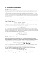
2.1 Estimation method
ISAS uses estimation theory for mapping of a scalar field on a regular grid from sparse and
irregular data (Bretherton et al.,1976). The interpolated field, represented by the state vector
x , is constructed as the departure from a reference field values at the grid points x f . This
reference is derived from previous knowledge (climatology or forecast). Only the unpredicted
part of the observation vector, or departure from the reference field at the data points, called
innovation, is used:
d = yo ! x f
The analyzed field x a , is obtained as a linear combination of the innovation, and is associated
with a covariance matrix P a .
!1
x a = x f + C ao (C o + R ) d ,
!1
T
(eq. 1)
P a = P f ! C ao (C o + R ) C ao
It should be noticed that this formalism provides at the same time an estimate of the misfit
between observations and analysis, also called analysis residuals:
!1
y o ! y ao = R (Co + R ) d
C ao is the covariance matrix between analyzed points and data points, C o is the covariance
matrix between data points and R is the error covariance matrix. It combines the measurement
error and the representativity error. The error on the estimation is given by the diagonal of the
P a matrix, usually normalized by the a priori variance.
T $
# Cao (Co + R )"1 Cao
! ei2
1
=
"
%
&
2
%
&
! xi2
!
xi
'
(ii
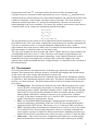
2.2 Statistical information
Statistical information on the field and data noise are introduced through the covariance
matrices that appear in equation 1. We assume that the covariances of the analyzed field can
be specified by a structure function modeled as the sum of two gaussians, the first term (i = 1)
corresponding to the large scale field (LS), the second (i = 2) to the mesoscale (MS):
" dx 2 dy 2 dt 2 #
2
2
C ( dx, dy , dt ) = ) i =1! i exp$ % 2 + 2 + 2 &
% 2L
&
' ix 2 Liy 2 Lit (
where dx, dy, dt are the space and time separation, Lix , Liy , Lit the corresponding e-folding
scales. The weight given to each ocean scale is controlled by the variances ! i2 .
The total variance is computed as the variance of the anomaly relative to the monthly
reference field. It is considered as the sum of four terms:
2
2
2
2
2
! tot
= ! LS
+ ! MS
+ ! UR
+ ! ME
2
2
where ! LS
and ! MS
are the two terms appearing in the equation for the covariance structure.
2
2
2
+ ! ME
The remaining sum ! UR
is the total error variance: ! ME
corresponds to the
8
2
measurement errors and ! UR
represents small scales unresolved by the analysis and
2
considered as noise, sometimes called representativity errors. A unique ! ME
profile has been
computed from the measurement errors of the standard database and substracted from the total
variance to obtain the ocean variance (first three terms of the sum). The ocean variance is
2
adjusted to remain larger than ! ME
and can be multiplied by a factor to account for the
under-sampling of the ocean variability. We express the variances associated to each scales as
a function of the ocean variance by introducing normalized weights:
2
! LS
= wLS! 2
2
! MS
= wMS! 2
2
! UR
= wUR! 2
wLS + wMS + wUR = 1
The free parameters of the system are the weights that define the distribution of variance over
the different scales. The error matrix combines the measurement error and the representativity
error due to unresolved scales, it is assumed diagonal, although this is only a crude
approximation since both errors are likely to be correlated for measurements obtained with the
same instrument, or within the same area and time period.
The large scale lengths are taken isotropic and equal to 300km, the target Argo resolution, the
corresponding time scale is set to 3 weeks. The meso-scale length is proportionnal to the
Rossby Radius computed from the annual climatology. In the equatorial band, this value is
bounded by the large scale length in the zonal direction, and by the length scale of the
adjacent zones in the meridional direction. At high latitudes, it is bounded by the resolution of
the estimation grid.
2.3 The datasets
We briefly describe here the characteristics of the data types taken into account at the
moment. These dataset have different accuracy, resolution and sampling that depend mostly
on the sensor and on the storage and transmission system used.
Temperature and salinity measurements are obtained from autonomous instruments, drifting
or anchored or from instruments deployed with a ship. The data are transmitted in real time by
satellite, or in delayed mode. The main characteristics of the most common instruments are
given below.
• Profiling floats: The autonomous floats are part of the ARGO program, they collect
vertical profiles of temperature and salinity as a function of pressure between their
maximum pressure (usually 2000 dbars) and the surface. At the end of the profile that
takes nearly 5 hours, the profiler transmits the data to a satellite and dives toward its
parking depth (1000 dbars), waiting for the next cycle (10 days later). Nominal
accuracy of the data is assumed to be 0.01°C and 0.01 PSU. At present time a vertical
profile is described by approximately 100 pts.
• XBT: An eXpendable BathyThermograph is launched from a steaming ship. It
measures temperature (and salinity in the case of XCTD) the measurement depth is
deduced from the XBT fall rate. The accuracy is 0.1°C and most XBT reach 800 m.
• CTD: This high quality measurement is obtained from a research vessel in the context
of a scientific cruise. Pressure and temperature sensors are carefully calibrated and
water samples are taken to adjust the salinity measurement. Standard procedure were
defined for the WOCE experiment, they lead to accuracies of 0.001°C and 0.001 PSU.
• Time series: Time series of pressure, temperature and salinity are recorded at high
time resolution (hours) from sensors installed on fixed points (mooring) or drifting
9
buoys. The measurement depth is usually constant. The sensors are similar to those
used on the profiling floats.
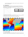
2.4 Configuration
The configuration proposed with ISAS-V4 is describred in detail in (Charraudeau and
Gaillard, 2007). The horizontal grid is ½ degree Mercator limited to 77S-77N. It is thus
isotropic and the resolution increases with latitude, from 0.5° at equator to 0.1125° à 77N.
The vertical levels are given below.
STD_LEVEL_A
STD_LEVEL_B
[[0 3] [5:5:100]
[110:10:800]
[820:20:2000]]
[[2020:20:2500]
[2550:50:5800]]
The bathymetry is an interpolation over our grid of the file etopo2bedmap.nc produced
by MERCATOR from the 2 minutes bathymetry file of the NGDG Bathy_Etopo2.nc.
The interpolation is done using the median of the 4 surrounding points.
2.5 Areas and masks
For the practical implementation of the method, the global ocean has been divided in areas,
that define the group of points to be processed at once. To each area, we associate a mask
10
defining the area where the information can be used. This allows for example to exclude the
Mediterranean while analysing the Gulf of Cadiz.
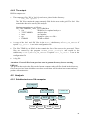
2.6 The analysis steps
The main processing steps are:
•
•
•
•
STD : Data with the valid quality control flag (QC) are selected from the raw data
files and interpolated on standard levels. A new flag, representing the quality of the
interpolation is associated with the each data.
PRE-OA : This pre-processing step gathers all data and statistical information that
will be used for the analysis of each area defined in the configuration.
OA: The analysis is performed over each area as described in the ‘method’ section
above.
POST-OA: This post-processing step gathers the results over each area to form the
full 3D field. Two files are produced, one holding the 3D fields and estimation error,
the other holding the data and residuals.
11
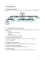
3 The directories
3.1 program directory
This directotory contains all programs required to perform the analysis. It is organized as
follows.
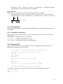
isas_v4.1
confstd
climref
aeradef
doc
isas_mat
_vname
std
preoa
isas_f90
postoa
perl
share
3.1.1 Configuration directory (confstd)
Contains all files defining the standard configurationused by the analysis (Charraudeau et
Gaillard, 2007):
• Bathymetry
• Climatology (annual and monthly)
• Variances
• Covariance scales
• Definition for analysis areas and masks.
3.1.2 Documentaion directory (doc)
Contient les documentations sur la description et la mise en oeuvre des programmes.
 ISAS_V4_config.pdf
 ISAS_V4_prog.pdf
3.1.3 Matlab scripts (isas_mat)
Contains the matlab scripts used for the standardisation, the pre- and post-processing.
3.1.4 Fortran programs (isas_f90)
Contains source codes, makefile and executable for the analysis.
3.1.5 Directory perl
Contains perl script that allow to loop over different analysis dates and parameters/
12
3.2 The data directories
La mise en oeuvre d’ISAS se base sur quatre répertoires principaux.
 Le répertoire ‘dir_raw/’ contient l’ensemble des données brutes fournies par Coriolis.
 Le répertoire ‘dir_confisas/’ contient les fichiers de configuration.
 Le répertoire ‘dir_resu/’ contient les résultats des analyses.
 Le répertoire ‘dir_run/’ contient les alertes, tracés, fichiers log et fichiers
intermédiaires des analyses.
Les deux premiers répertoires sont fournis par l’utilisateur, les deux autres sont crées par
l’analyse.
3.3 Répertoire raw : les données brutes
Ce dossier est préparé par l’utilisateur et doit respecter l’organisation qui suit. Contient un
sous répertoire par lot de données homogènes, issues d’un même fournisseur. A l’intérieur
d’un sous répertoire, les données sont organisées par année
La dénomination des fichiers suit la convention de la documentaion Coriolis (Antonio, 2007).
Un niveau ‘mois/bassin’ a été conservé pour assurer la compatibilité avec l’organisation
précédente, mais son usage n’es pas recommandé.
3.4 Répertoire confisas
Contient le fichier de configuration de l’analyse pour définir les chemins et l’ensemble des
paramètres ajustables de l’analyse. Un exemple de fichiers figure dans le répertoire
doc/config_model.
 isas_matlab.env : chemins matlab
 oa_config_isas.txt : fichier de configuration définissant les paramètres des
programmes matlab tel qu’il sera lu par isas_mat
 TEMP_6_2006.in, TEMP.cnf, PSAL.cnf : modèles de fichiers de
configuration pour les programmes f90, à recopier dans le répertoire f90 correspondant.
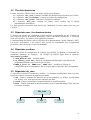
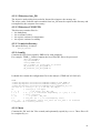
3.5 Répertoire dir_resu
Ce répertoire contient les résultats de l’analyse. Ces résultats sont distribués dans trois sousrépertoires, chacun contenant un répertoire par année.
 std : fichiers contenant les données sur niveau standard, ces fichiers correspondent
aux fichiers ‘raw’ mais peuvent être regroupés par mois
 field : Fichiers contenant les champs analysés sur la grille régulière
 data : fichiers contenant les données utilisées pour le calcul du champ ‘field’ ainsi que
les résidus d’analyse.
Dir_resu
std
data
Field
13
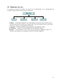
3.6 Répertoire dir_run
Ce répertoire contient les fichiers de travail et les informations sur le déroulement de
l’analyse. Ils peuvent être effacés après vérification.
Dir_run
alert
logisas
plotisas
preoa
 alert : Contient un répertoire ‘list’ qui regroupe les listes d’alertes émises par les
différents niveaux de traitement et un répertoire ‘std’ qui contient les tracés des profils
détectés en alerte par le programme STD_main
 logisas : contient les fichiers logs produits par les différentes étapes
 plotisas : contient les tracés produits par les différentes étapes
 preoa : Contient fichiers ‘fld’ et ‘dat’ par zones préparés par PREOA_main. Ces
fichiers sont recopiés sur la machine de calcul où ils sont complétés.
14
4 Processing an anlysis
4.1 Matlab path
Before starting the analysis, the matlkab path need to be defined. The environment is
described in a file isas_matlab.env that we recommend be placed in the directory
confisas/. See isas_v4/doc/config for an example.
To launch, type:
cd confisas
source ISAS_matlab.env
#!/usr/bin/sh
#
#
#
----------------------------------------------Matlab directory:
-----------------------------------------------
setenv MATHOME
setenv TOOLBOXPATH
setenv ISAS_HOME
/home/machine/matlab_dir/matlab_r2007b
/home/machine/matlab_dir/outils_matlab/m_map1.4
/home/machine/isas_dir
setenv OA_HOME ${ISAS_HOME}/isas_v4.1/isas_mat_4.1b
setenv OA_PATH
${OA_HOME}/std:${OA_HOME}/preoa:${OA_HOME}/postoa:${OA_HOME}/share
setenv MATLABPATH ${OA_PATH}:${TOOLBOXPATH}
setenv MATLAB ${MATHOME}:${MATHOME}/bin:${MATHOME}/etc
set path=($MATLAB $path)
alias matlab
'${MATHOME}/bin/matlab'
15
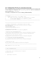
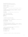
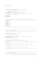
4.2 Configuration file for pre- and post-processing
Before starting the analysis, the various path, file names and parameters must be defined. This
is done through the configuration file: oa_config_isas.txt, that we recommend be
placed in the directory : confisas/.
An example of configuration file is given in isas_v4/doc/config
%==========================================================================
% Warning :
%
Lines starting with % are comment lines
%
the others are read to define the configuration, on those:
%
do not leave spaces if not required by syntax
%
do not write comments
%==========================================================================
%=============================================================
% Standart configuration : directories and file names
DIR_CONFSTD=/home/machine/dir-run/isas/isas_v4.1/confstd/
nam_clim=ISASW_4
nam_std=ISASW_52_STD
nam_bathy=bathy_GLOBAL05_V4_0.nc
% Directory for raw data
DIR_RAW_ROOT=/home7/machine/raw_data/CO_DMQCGL01/
% Directory dor standardized data
% note that a same std dataset can be used for different analysis
DIR_STD_ROOT=/home/machine/dir-run/ana/arragl03/ISAS_RESU/std/
% Directory for the analysis results
DIR_ANA_RESU=/home/machine/dir-run/ana/arragl05/ISAS_RESU/
% Directory for the analysis processing
%
(log files, plots, temporary files)
DIR_ANA_RUN=/home/machine/dir-run/ana/arragl05/ISAS_RUN/
% directory for f90
DIR_OA_CALCUL=/home2/computer/user/OA/run/arragl05/
%===================================================================
AREA_LIMITS=[-81 +80 -180 +180]
%===================================================================
% STD: Standardisation
%===================================================================
% ocean_list: list of directories to explore
DIR_RAW_LIST=none
%
Specifique 'Coriolis'
16
%-----------------------% TYP_LIST: List of file types to process
TYP_LIST=PR_TE,PR_XB,PR_CT,PR_MO,PR_PF,PR_BA
% PRF_RAW
: identifier for raw files,
PRF_RAW=CO_DMQCGL01_
% PRF_STD : identifier for STD files,
PRF_STD=ST_DMQCGL01_
% month_grp=1
month_grp=1
: all data within a month are grouped, no group = 0
% all RAW data from different basins are grouped in a single STD
% needed for compatibility with previous versions of Coriolis
% file naming convention
ocean_grp=1
% use_adjust=1
use_adjust=0
: use adjusted value if exist (else: =0)
% QC_TS: flags ok Temp and Psal
% QC_ZP: flags ok Pres and depth
%fQC_XY: flags ok Position and date
QC_TS=125
QC_ZP=0 125
QC_XY=0 125
%
%
Parameter for the profile control
----------------------------------
% Criteria for comparing to climatology :
% crit_std_clim : number of standard deviation allowed relative to
% the climatology
%crit_std_clim=8 % first pass
%crit_std_clim=15 % second pass
crit_std_clim=15
%
%
%
%
alpha_clim : Stratification correction
A correction proportionnal to the vertical gradient is added to
the standard deviation. If alpha_clim=0.6, we allow an additional
0.6*(dT/dZ or dS/dZ) distance to climatology
alpha_clim=2
% Criteria for spike detection based on second derivative
% Small value detects smaller spikes
%crit_spike_temp = 200 %
first pass
%crit_spike_psal = 200
%crit_spike_temp = 800 %
second pass
%crit_spike_psal = 800
crit_spike_temp = 800
crit_spike_psal = 800
%
INT_NB_MIN : Min number of points to perform interpolation
17
INT_NB_MIN=2
% Parameters for reduction of nearby profiles
% (creates ‘super profiles’:
% --------------------------------------------% RED_DXMAX: max distance (in km)
% RED_DTMAX: max time interval (in days)
% RED_QCMAX: QC max (defined by STD preocess) used to build
%
the superprofiles
RED_DXMAX=15
RED_DTMAX=7
RED_QCMAX=4
% Definition of default errors associated to each data type.
% will be used only if no error is specified within the raw data file
TE_ERR=0.03
BA_ERR=0.05
PF_ERR=0.01
XB_ERR=0.03
CT_ERR=0.01
MO_ERR=0.01
BH_ERR=0.002
%===================================================================
%===================================================================
% PREOA: Preprocessing
%===================================================================
% May be used to overwrite STD name
%PRF_STD=ST_RAOAGL01_
% Instrument type excluded
%INST_EXCL_LIST=[(1:800),900] : exclude XBTs of all types
%INST_EXCL_LIST=[]
INST_EXCL_LIST=[(1:800),900]
% List of areas to be analyzed
ANA_AREA_LIST=[101:141,201:241,301:388,401:403];
%time interval (in days) (look within day – AMPL_OA and day + AMPL_OA
AMPL_OA=30
% Copies NetCDF files on the fortran computer (DIR_OA_CALCUL)
copy_preoa=1
% Creates the input file for the fortran computer
creat_in_preoa=1
%===================================================================
%===================================================================
% POSTOA: Post-Processing
%===================================================================
% AR = Arivo, RA = Re-analysis, AT=Atlantic, X1: analysis identifier
18
ANA_NAME=arragl05
% Reference climatology : month or year
% clim_ref_oa=M (month) or clim_ref_oa=Y (year)
clim_ref_oa=M
% Spatial filtering on areas boundaries applied on points
% with err>err_max
filter_err_max=80
%===================================================================
%data set
DATA_SET=CO_DMQCGL01
%product version
PRODUCT_VERSION=arragl05
%Project name
PROJECT_NAME=ARIVO
%Data manager
DATA_MANAGER=Fabienne Gaillard
%plot % Plot options(0 =no plots, 3 = maxplots + pause)
PLOT_CONV=1
LANG=En
4.3 Standardisation
4.3.1 Description
The first step in the analysis is an interpolation of the raw data on the standard levels of the
analysis grid. It is partly independent of the analysis, in the sense that the dataset produced
can be used for different analysis. A new QC is introduced, it represents the quality of the
interpolation (the closest to a measured value the lowest the QC flag value).
To avoid spoiling the analysis with eroneous data, a control is performed before the
interpolation. Finally, oversampled points such as repeated fixed points CTD, drfting buoys,
mooring can be averaged (reduced) into super-profiles. Each of these procesing are detailled
below.
4.3.1.1 Detection of erroneous data
Two different test are succesively applied:
Distance to climatology:
A data point will be accepted if the value X verifies: Xobs – Xclim < α1 STD + α2 δX/δz
 The scalar α1 (crit_stdin the configuration file) has been determined empirically, it
defines the distance allowed to the climatology.
 The scalar α2 introduces an additional tolerance relative to the climatology. In the
vicinity of very strong stratification, perfectly good data may differ strongly from the
19
climatology. This is taken into account by introducing an additional tolerance
proportional to the vertical gradient of the parameter.
Spike detection:
A data value is considered as a spike if the following conditions are filled:
 Change of sign of the first derivative for at least one point before or after the point.
 Second derivative criteria normalized by the median in the vicinity of the point:
" 2P
( z)
"z 2
! crit _ spike
" 2P
mediane(
)
"z
4.3.1.2 Interpolation
The high resolution data are bin averaged on the standard levels, then the remaining levels are
interpolated
4.3.1.3 Reduction (superobs)
Data from the same platform which are close in time and space are averaged. The control
parameters are :
RED_DXMAX : Minimum distance in kilometers
RED_DTMAX : minimum time difference in days
RED_QCMAX : maximum QC-flag (after standardisation)
4.3.2 Running STD
After setting the parameters of the STD block in the configuration file, STD_main can be
launched in the matlab execution window.
config_fname = ’my_analysis/confisas/OA_config_ISAS.txt/’;
% to process 10 days starting on july 14, 2006:
dd = 14;
mm = 07;
yyyy = 2006;
nb_days = 10;
% To process a full month (ex july 2006)
dd = 0;
mm = 07;
yyyy = 2006;
nb_days = 0; % or anything, this value is ignored
STD_main (config_fname, [dd mm yyyy], nb_days);
An example of perl script to run STD_main over several month and years is given in
/isas_v4/perl/std
Type:
perl std.pl
20
4.3.3 Outputs
4.3.3.1 Data files on standard levels
Results are writen as NetCDF files in the directory : dir_resu/std/. The naming
convention is as follows :
ST_CCCCCCCC_YYYYMMDD_PR_YY.nc
• ST
identifies « STD » data
• CCCCCCCC
dataset name
• YYYYMMDD
date of observation, if day = 00, file contains the whole month
• PR
identifies « profile» data
• YY
data types according to Coriolis convention
4.3.3.2 Listing (log file):
The log file can be found in dir_run /logisas/
Example of log file:
>>>>>>>
Running ISAS_V4.0/STD
Last update :18-Apr-2007 18:27:25
------------------------------------STD: Type PR_TE, 31 files found
------------------------------------******** File
1 ********
File processed:
CO_TST_20040701_PR_TE
Number of profiles read :
3
Number of valid profiles (QC_posdate):3
Number of profiles kept:
3
Number of profiles per type:
T: 0, S: 0, TS: 3, total 3
Number of profiles without depth: 1
Number of profiles per type:
T: 0, S: 0, TS: 3, total 3
3 profiles, CPU time total (seconds): 16.20
CPU read:
1.76, depth:
1.48, STD check: 10.53, Stdlev:
1.62
…
******** File
31 ********
File processed:
CO_TST_20040731_PR_TE
Number of profiles read :
18
Number of valid profiles (QC_posdate):18
Number of profiles kept:
18
Number of profiles per type:
T: 6, S: 0, TS: 12, total 18
Number of profiles without depth: 12
Number of profiles per type:
T: 6, S: 0, TS: 12, total 18
18 profiles, CPU time total (seconds): 18.40
CPU read:
0.96, depth:
1.77, STD check: 14.41, Stdlev:
1.94
112 Multiple profiles
platform: 13009
, nb_av: 2
platform: 13009
, nb_av: 2
platform: 15001
, nb_av: 2
…
platform: CGDV
, nb_av: 3
platform: CGDV
, nb_av: 2
Final number of profiles per type: 261
T: 35, S: 0, TS: 226
processing time - red:
1.53, prep:
0.05, write:
6.00
21
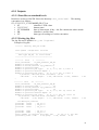
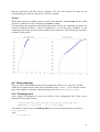
4.3.3.3 Control plots
Different types of plots can be found in dir_run/plotisas/std.
Standard plot level (PLOT_CONV=1) :
A plot showing all profiles is produced.
High level plot (PLOT_CONV>1) :
Additional plots are saved in the subdirectory ‘ctrl’ for one profile of the group, showing in
blue the raw data, in red the interpolated data, in green the interpolated data with QC higher
22
than the threshold, and that will be excluded. The plot title include the name of the
corresponding raw data file, and the DC_reference number.
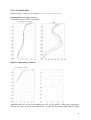
Alertes
When data points are excluded, a plot is created in the directory : alert/std and the profile
reference is added to the list in the directory alert/list.
The plot shows the temperature and salinity data points in blue, the climatology in black, the
corrected standard deviation criteria as dashed line. In red, the points excluded by the
climatology test and in green the points ecluded by the spike test. The plot title gives the DCreference of the profile.
4.4 Preprocessing
PRE_OA select the data that will be used to perform the analysis over each area. All data
within the area mask and the time interval defined by date +/-AMPL_OA are selected. At this
stage, data might be excluded on the instrument type criteria (INST_EXCL_LIST).
4.4.1 Running preoa
After setting the parameters in the preoa block of the configuration file. Preoa can be
launched in the matlab window.
config_fname=myanalysis/prepana/confisas/OA_config_ISAS.txt/’;
PREOA_main( config_fname , [15 01 2006],’TEMP’)
An example of perl script to run PREOA_main over several month and years is given in
/isas_v4/perl/
Type:
perl preoa.pl
23
4.4.2 The output
PREOA outputs are :
•
The temporary files ’fld’ et ’dat’ for each area, placed in the directory:
dir_run /preoa /
The ’fld’ files contain the empty anomaly filed for the area on the grid. The ’dat’ files
contain the data to be used by the analysis.
Naming convention are as follows :
OA_YYYYMMDD _ iarea _typ_PARAM.nc
• OA
identifier for «optimal analyse »
• YYYYMMDD
analysis date
• iarea
area number
• typ
identifier «dat » ou « fld »
• PARAM
TEMP ou PSAL

A copy of the ‘dat’ and ‘fld’ files in the data/ subdirectory of DIR_OA_CALCUL if
option copy_preoa=1 is set in the configuration file

The files TEMP.in, ou PSAL.in that contain the list of the areas to be processed. These
files are created by the program PREOA_creat_configin and copied in the
subdirectory config of DIR_OA_CALCUL if option creat_in_preoa=1 is set in the
configuration file

A log file
Attention : Erase all files from previous runs in preoa directory berore running
PREOA !
The process that copies the files on the fortran computer takes all files found in the directory,
files from previous runs which have not been overwritten will be taken into acount and may
produce inconsistencies..
4.5 Analysis
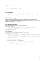
4.5.1 Subdirectories on OA-computer
OA_computer
Dir_oa_calcul
isas_f90
data
config
batch
log
err
2006
2006
TEMP
CONFSTD
PSAL
TEMP
PSAL
24
4.5.1.1 Directory isas_f90
The objective analysis has been coded in fortran 90 to improve the memory use.
The source codes, makefile and executable from isas_f90 must be copied in this directory and
recompiled for the computer if necessary.
4.5.1.2 Directory CONFSTD
This directory contains files for :
• the bathymetry
• the covariance scales
• the a priori variance for temperature
• the a priori variance for salinity
4.5.1.3 Analysis directory
The parent directory is named:
DIR_OA_CALCUL
4.5.1.4 config
Contains the list of area copied by PREOA for each parameter.
For example: TEMP_1_2006.in contains the list of NetCDF files to be processed:
data/2006/TEMP/$
log/2006/TEMP/$
config/TEMP.cnf$
164 % number of files/area to process
OA_20060101_101_dat_TEMP.nc
OA_20060101_102_dat_TEMP.nc
…
It should also contain the configuration file for the analysis (TEMP.cnf or PSAL.cnf)
TEMP
/home2/mycomputer/user/OA/run/CONFSTD/ISASW_52_STD_TEMP.nc
/home2/mycomputer/user/OA/run/CONFSTD/ISASW_4_ann_COVS.nc
/home2/mycomputer/user/OA/run/CONFSTD/bathy_GLOBAL05_V4_0.nc
300 300 21 % covar_ls x, y t (in km, km, days)
21
% covar_ms_t (in days)
1 1 4
% var_weigh (LS, MS, UR)
1 1 0 1
% x, y, z, t covariance dependency (1 = yes, 0 = no)
1.2
% fact. Variance
2 12
% QC Max
Mx_std
1.1
% Cov_max (if > 1, no oversampling test)
3.5
11
% oversample: alpha, fct_test (Si fct_test < 10 autorise
l'augment. de l'erreur partout)
4.5.1.5 data
Contains the ‘fld’ and ‘dat’ files created (and optionnally copied) by PREOA. Those files will
be completed by OA.
25
4.5.2 Running ISAS_f90
The program can be run in interactive mode :
cd my_analysis_f90
calculateur/isas_f90/OA_main
<
config/TEMP_2006.in
It can also be launched in batch mode, this allows to loop over dates and parameters.
The way batches are run is machine dependent. Examples are given here for SGI – ICE 8200.
Launch with:
qsub my_batch
where my_batch contains:
#!/bin/csh
# get the path for library MKL
source /usr/share/modules/init/csh
module load cmkl/recent
setenv MKL_SERIAL YES
cd my_analysis_f90
foreach year (2003 2004 2005 2006)
foreach month (1 2 3 4 5 6 7 8 9 10 11 12)
foreach param (TEMP PSAL)
date
calculateur/isas_f90/OA_main < config/$param\_$month\_$year\.in
date
end
end
end
4.5.3 Outputs
4.5.3.1 err
Contains a short log file with the list of processes files and any error message issued by the
program. This file must be screened carafully to chck that the processing has ended normally.
4.5.3.2 log
The log file contain statistical information on the processing for each area and each level of
analysis.
*****
Area:
218,
Nb_profiles:
Nb_level:
Nb_analysis points: (nlon,nlat):
cpu distance calculations:
85
152
24
28
0.038
Level:
1, Nb_ana_points:
535, Nb_ovsamp:
0, Nb_data:
ano_max: 11.892, inov min: -2.729, inov max:
1.526
fld min: -1.566, fld max: -0.076
cond #
0.4999E+00,
cpu Analysis: 0.006
58
Level:
2, Nb_ana_points:
535, Nb_ovsamp:
0, Nb_data:
ano_max: 11.892, inov min: -2.677, inov max:
1.478
fld min: -1.527, fld max: -0.096
cond #
0.5000E+00,
cpu Analysis: 0.006
58
26
Level:
3,...
...
*****
cpu total area:
1.582
4.5.3.3 data files
The analysis results are store in the ‘fld’ and ’dat’ data files that now contain the gridded
anomaly fields and corresponding error and the data residuals, respectively.
4.6 Post-Processing
During this last part of the processing, POSTOA concatenates all processed areas and
datasets. It also convert anomalies to absolute values. The files are read in DIR_OA_CALCUL
and results are written in DIR_ANA_RESU
.
4.6.1 Running POSTOA
POSTOA is launched with the same arguments as PREOA :
In the matlab window :
config_fname=myanalysis/prepana/confisas/OA_config_ISAS.txt/’;
POSTOA_main( config_fname , [15 01 2006],’TEMP’)
Perl script are also provided.
4.6.2 Outputs
The processing can be checked looking at the log files and plots.
The results are saved in two files:
 In {DIR_ANA_RESU}/data, the NetcCDF ‘dat’ file that contains the data and
residuals used by all the areas .
 In {DIR_ANA_RESU}/field the NetCDF file ‘fld’ that contains the global 3D
gridded fields and error.
File naming convention are as follows :
nameana_YYYYMMDD _ typ_PARAM.nc
• nameana
analysis identifier (ANA_NAME in the config file)
• YYYYMMDD analysis day
• PR
identifier «dat » ou « fld »
• PARAM
TEMP or PSAL
27
5 References
Antonio, J. 2007: Outils d’analyse de données in-situ (ISAS), formats et nomenclatures en
version 3.7. Document provisoire Coriolis.
Gaillard, F. et E. Autret, 2006 : Climatologie et statistique de l’Atlantique Nord. Projet
GMMC 2003.
Bretherton, F., R. Davis, and C. Fandry, (1976), A technique for objective analysis and design
of oceanic experiments applied to Mode-73. Deep Sea Research, 23, 1B, 559--582.
Charraudeau, R. et F. Gaillard, 2007 : ISAS_V4 : Mise en place de la configuration, Rapport
LPO 07-09, 88 p.
28
6 Annex
6.1 STD file
%% ncdump('ST_RAOAGL01_20020100_PR_PF.nc')
10:47:32
%% Generated 23-Nov-2007
nc = netcdf('ST_RAOAGL01_20020100_PR_PF.nc', 'noclobber');
if isempty(nc), return, end
%% Global attributes:
nc.Last_update = ncchar(''05-Nov-2007 17:01:58'');
nc.SoftwareVersion = ncchar(''ISAS_V4.03/STD'');
%% Dimensions:
nc('DATE_TIME') = 14;
nc('STRING256') = 256;
nc('STRING64') = 64;
nc('STRING32') = 32;
nc('STRING16') = 16;
nc('STRING8') = 8;
nc('STRING4') = 4;
nc('STRING2') = 2;
nc('N_PROF') = 930;
nc('N_LEVELS') = 152;
nc('RP_NB_PROF') = 995;
%% Variables and attributes:
nc{'DATA_TYPE'} = ncchar('STRING16'); %% 16 elements.
nc{'DATA_TYPE'}.comment = ncchar(''Data type'');
nc{'FORMAT_VERSION'} = ncchar('STRING4'); %% 4 elements.
nc{'FORMAT_VERSION'}.comment = ncchar(''File format version'');
nc{'REFERENCE_DATE_TIME'} = ncchar('DATE_TIME'); %% 14 elements.
nc{'REFERENCE_DATE_TIME'}.comment = ncchar(''Date of reference for Julian
days'');
nc{'REFERENCE_DATE_TIME'}.conventions = ncchar(''YYYYMMDDHHMISS'');
nc{'PI_NAME'} = ncchar('N_PROF', 'STRING64'); %% 59520 elements.
nc{'PI_NAME'}.comment = ncchar(''Name of the principal investigator'');
nc{'PLATFORM_NUMBER'} = ncchar('N_PROF', 'STRING8'); %% 7440 elements.
nc{'PLATFORM_NUMBER'}.long_name = ncchar(''Float unique identifier'');
nc{'PLATFORM_NUMBER'}.conventions = ncchar(''WMO float identifier:
QA9IIIII'');
nc{'CYCLE_NUMBER'} = nclong('N_PROF'); %% 930 elements.
nc{'CYCLE_NUMBER'}.long_name = ncchar(''Float cycle number'');
nc{'CYCLE_NUMBER'}.conventions = ncchar(''0..N, 0 : launch cycle (if
exists), 1 : first complete cycle'');
nc{'CYCLE_NUMBER'}.FillValue_ = nclong(99999);
nc{'DIRECTION'} = ncchar('N_PROF'); %% 930 elements.
29
nc{'DIRECTION'}.long_name = ncchar(''Direction of the station profiles'');
nc{'DIRECTION'}.conventions = ncchar(''A: ascending profiles, D: descending
profiles'');
nc{'DATA_CENTRE'} = ncchar('N_PROF', 'STRING2'); %% 1860 elements.
nc{'DATA_CENTRE'}.long_name = ncchar(''Data centre in charge of float data
processing'');
nc{'DATA_CENTRE'}.conventions = ncchar(''GTSPP table'');
nc{'DC_REFERENCE'} = ncchar('N_PROF', 'STRING32'); %% 29760 elements.
nc{'DC_REFERENCE'}.long_name = ncchar(''Station unique identifier in data
centre'');
nc{'DC_REFERENCE'}.conventions = ncchar(''Data centre convention'');
nc{'DATA_STATE_INDICATOR'} = ncchar('N_PROF', 'STRING4'); %% 3720 elements.
nc{'DATA_STATE_INDICATOR'}.long_name = ncchar(''Degree of processing the
data have passed through'');
nc{'DATA_STATE_INDICATOR'}.conventions = ncchar(''OOPC table'');
nc{'DATA_MODE'} = ncchar('N_PROF'); %% 930 elements.
nc{'DATA_MODE'}.long_name = ncchar(''Delayed mode or real time data'');
nc{'DATA_MODE'}.conventions = ncchar(''R : real time; D : delayed mode'');
nc{'INST_REFERENCE'} = ncchar('N_PROF', 'STRING64'); %% 59520 elements.
nc{'INST_REFERENCE'}.long_name = ncchar(''Instrument type'');
nc{'INST_REFERENCE'}.conventions = ncchar(''Brand, type, serial number'');
nc{'WMO_INST_TYPE'} = ncchar('N_PROF', 'STRING4'); %% 3720 elements.
nc{'WMO_INST_TYPE'}.long_name = ncchar(''Coded instrument type'');
nc{'WMO_INST_TYPE'}.conventions = ncchar(''WMO code table 1770 - instrument
type'');
nc{'JULD'} = ncdouble('N_PROF'); %% 930 elements.
nc{'JULD'}.long_name = ncchar(''Julian day (UTC) of the station relative to
REFERENCE_DATE_TIME'');
nc{'JULD'}.units = ncchar(''days since 1950-01-01 00:00:00 UTC'');
nc{'JULD'}.conventions = ncchar(''Relative julian days with decimal part
(as parts of day)'');
nc{'JULD'}.FillValue_ = ncdouble(999999);
nc{'LATITUDE'} = ncdouble('N_PROF'); %% 930 elements.
nc{'LATITUDE'}.long_name = ncchar(''Latitude of the station, best
estimate'');
nc{'LATITUDE'}.units = ncchar(''degree_north'');
nc{'LATITUDE'}.FillValue_ = ncdouble(99999);
nc{'LATITUDE'}.valid_min = ncdouble(-90);
nc{'LATITUDE'}.valid_max = ncdouble(90);
nc{'LONGITUDE'} = ncdouble('N_PROF'); %% 930 elements.
nc{'LONGITUDE'}.long_name = ncchar(''Longitude of the station, best
estimate'');
nc{'LONGITUDE'}.units = ncchar(''degree_east'');
nc{'LONGITUDE'}.FillValue_ = ncdouble(99999);
nc{'LONGITUDE'}.valid_min = ncdouble(-180);
nc{'LONGITUDE'}.valid_max = ncdouble(180);
nc{'DEPH'} = ncfloat('N_LEVELS'); %% 152 elements.
nc{'DEPH'}.long_name = ncchar(''Depth'');
nc{'DEPH'}.units = ncchar(''meter'');
nc{'DEPH'}.FillValue_ = ncfloat(99999);
nc{'DEPH'}.valid_min = ncdouble(0);
30
nc{'DEPH'}.valid_max = ncdouble(10000);
nc{'TEMP'} = ncfloat('N_PROF', 'N_LEVELS'); %% 141360 elements.
nc{'TEMP'}.FillValue_ = ncfloat(99999);
nc{'TEMP'}.long_name = ncchar(''Ocean temperature (T90) (interpolated on Z
levels)'');
nc{'TEMP'}.units = ncchar(''degree_Celsius'');
nc{'TEMP'}.valid_min = ncfloat(-3);
nc{'TEMP'}.valid_max = ncfloat(40);
nc{'TEMP_ERR_ME'} = ncfloat('N_PROF', 'N_LEVELS'); %% 141360 elements.
nc{'TEMP_ERR_ME'}.FillValue_ = ncfloat(99999);
nc{'TEMP_ERR_ME'}.long_name = ncchar(''Error on interpolated
temperature'');
nc{'TEMP_ERR_ME'}.units = ncchar(''degree_Celsius'');
nc{'TEMP_ERR_ME'}.valid_min = ncfloat(0.00100000004749745);
nc{'TEMP_ERR_ME'}.valid_max = ncfloat(10);
nc{'TEMP_CLIM'} = ncfloat('N_PROF', 'N_LEVELS'); %% 141360 elements.
nc{'TEMP_CLIM'}.FillValue_ = ncfloat(99999);
nc{'TEMP_CLIM'}.long_name = ncchar(''Climatology reference of profile'');
nc{'TEMP_CLIM'}.units = ncchar(''degree_Celsius'');
nc{'TEMP_CLIM'}.valid_min = ncfloat(-3);
nc{'TEMP_CLIM'}.valid_max = ncfloat(40);
nc{'TEMP_CLIM_STD'} = ncfloat('N_PROF', 'N_LEVELS'); %% 141360 elements.
nc{'TEMP_CLIM_STD'}.FillValue_ = ncfloat(99999);
nc{'TEMP_CLIM_STD'}.long_name = ncchar(''Standard deviation of climatology
reference of profile'');
nc{'TEMP_CLIM_STD'}.units = ncchar(''degree_Celsius'');
nc{'TEMP_CLIM_STD'}.valid_min = ncfloat(0);
nc{'TEMP_CLIM_STD'}.valid_max = ncfloat(40);
nc{'TEMP_QC'} = ncchar('N_PROF', 'N_LEVELS'); %% 141360 elements.
nc{'TEMP_QC'}.FillValue_ = ncchar(''0'');
nc{'TEMP_QC'}.conventions = ncchar(''Q where Q =[0-9]'');
nc{'TEMP_QC'}.long_name = ncchar(''Quality on interpolated temperature'');
nc{'PSAL'} = ncfloat('N_PROF', 'N_LEVELS'); %% 141360 elements.
nc{'PSAL'}.FillValue_ = ncfloat(99999);
nc{'PSAL'}.long_name = ncchar(''Salinity (S78) (interpolated on Z
levels)'');
nc{'PSAL'}.units = ncchar(''PSU'');
nc{'PSAL'}.valid_min = ncfloat(0);
nc{'PSAL'}.valid_max = ncfloat(60);
nc{'PSAL_ERR_ME'} = ncfloat('N_PROF', 'N_LEVELS'); %% 141360 elements.
nc{'PSAL_ERR_ME'}.FillValue_ = ncfloat(99999);
nc{'PSAL_ERR_ME'}.long_name = ncchar(''Error on interpolated salinity'');
nc{'PSAL_ERR_ME'}.units = ncchar(''PSU'');
nc{'PSAL_ERR_ME'}.valid_min = ncfloat(0.00100000004749745);
nc{'PSAL_ERR_ME'}.valid_max = ncfloat(10);
nc{'PSAL_CLIM'} = ncfloat('N_PROF', 'N_LEVELS'); %% 141360 elements.
nc{'PSAL_CLIM'}.FillValue_ = ncfloat(99999);
nc{'PSAL_CLIM'}.long_name = ncchar(''Climatology reference of profile'');
nc{'PSAL_CLIM'}.units = ncchar(''PSU'');
nc{'PSAL_CLIM'}.valid_min = ncfloat(0);
nc{'PSAL_CLIM'}.valid_max = ncfloat(60);
nc{'PSAL_CLIM_STD'} = ncfloat('N_PROF', 'N_LEVELS'); %% 141360 elements.
31
nc{'PSAL_CLIM_STD'}.FillValue_ = ncfloat(99999);
nc{'PSAL_CLIM_STD'}.long_name = ncchar(''Standard deviation of climatology
reference of profile'');
nc{'PSAL_CLIM_STD'}.units = ncchar(''PSU'');
nc{'PSAL_CLIM_STD'}.valid_min = ncfloat(0);
nc{'PSAL_CLIM_STD'}.valid_max = ncfloat(60);
nc{'PSAL_QC'} = ncchar('N_PROF', 'N_LEVELS'); %% 141360 elements.
nc{'PSAL_QC'}.FillValue_ = ncchar(''0'');
nc{'PSAL_QC'}.conventions = ncchar(''Q where Q =[0-9]'');
nc{'PSAL_QC'}.long_name = ncchar(''Quality on interpolated salinity'');
nc{'RP_DC_REFERENCE'} = ncchar('RP_NB_PROF', 'STRING32'); %% 31840
elements.
nc{'RP_DC_REFERENCE'}.long_name = ncchar(''DC_reference of raw profiles'');
nc{'RP_DC_REFERENCE_R'} = ncchar('RP_NB_PROF', 'STRING32'); %% 31840
elements.
nc{'RP_DC_REFERENCE_R'}.long_name = ncchar(''DC_reference of STD
profiles'');
nc{'RP_TEMP_QC_STD'} = ncchar('RP_NB_PROF'); %% 995 elements.
nc{'RP_TEMP_QC_STD'}.long_name = ncchar(''Temperature QC flag from STD '');
nc{'RP_PSAL_QC_STD'} = ncchar('RP_NB_PROF'); %% 995 elements.
nc{'RP_PSAL_QC_STD'}.long_name = ncchar(''Salinity QC flag from STD'');
6.2 Field file
%% ncdump('arragl02_20020115_fld_TEMP.nc')
10:43:41
%% Generated 23-Nov-2007
nc = netcdf('arragl02_20020115_fld_TEMP.nc', 'noclobber');
if isempty(nc), return, end
%% Global attributes:
nc.CONVENTIONS = ncchar(''COARDS'');
nc.producer_agengy = ncchar(''IFREMER'');
nc.project_name = ncchar(''ARIVO'');
nc.creation_time = ncchar(''20071123T102406'');
nc.software_version = ncchar(''ISAS_V4.0/POSTOA'');
nc.product_version = ncchar(''ARRAGL02'');
nc.data_set = ncchar(''arragl02'');
nc.data_manager = ncchar(''Fabienne Gaillard'');
nc.estimate_date = ncchar(''20020115'');
nc.south_latitude = ncchar(''-77.0105'');
nc.north_latitude = ncchar(''77.1224'');
nc.west_longitude = ncchar(''-180'');
nc.east_longitude = ncchar(''179.5'');
%% Dimensions:
nc('time') = 1;
nc('depth') = 152;
nc('latitude') = 500;
nc('longitude') = 720;
%% Variables and attributes:
32
nc{'time'} = ncfloat('time'); %% 1 element.
nc{'time'}.units = ncchar(''days since 1950/01/01 UTC 00:00:00'');
nc{'latitude'} = ncfloat('latitude'); %% 500 elements.
nc{'latitude'}.units = ncchar(''degree_north'');
nc{'latitude'}.valid_min = ncfloat(-90);
nc{'latitude'}.valid_max = ncfloat(90);
nc{'longitude'} = ncfloat('longitude'); %% 720 elements.
nc{'longitude'}.units = ncchar(''degree_east'');
nc{'longitude'}.valid_min = ncfloat(-180);
nc{'longitude'}.valid_max = ncfloat(180);
nc{'depth'} = ncshort('depth'); %% 152 elements.
nc{'depth'}.units = ncchar(''m'');
nc{'depth'}.positive = ncchar(''down'');
nc{'depth'}.valid_min = ncshort(0);
nc{'depth'}.valid_max = ncshort(2000);
nc{'TEMP'} = ncshort('time', 'depth', 'latitude', 'longitude'); %% 54720000
elements.
nc{'TEMP'}.long_name = ncchar(''Temperature'');
nc{'TEMP'}.units = ncchar(''degree_Celsius'');
nc{'TEMP'}.valid_min = ncfloat(-23000);
nc{'TEMP'}.valid_max = ncfloat(20000);
nc{'TEMP'}.FillValue_ = ncshort(32767);
nc{'TEMP'}.add_offset = ncfloat(20);
nc{'TEMP'}.scale_factor = ncfloat(0.00100000004749745);
nc{'TEMP'}.comment = ncchar(''Estimated by optimal interpolation'');
nc{'pct_variance'} = ncshort('time', 'depth', 'latitude', 'longitude'); %%
54720000 elements.
nc{'pct_variance'}.long_name = ncchar(''Error on temperature (percent
variance)'');
nc{'pct_variance'}.units = ncchar(''percent of a priori variance'');
nc{'pct_variance'}.valid_min = ncfloat(0);
nc{'pct_variance'}.valid_max = ncfloat(100);
nc{'pct_variance'}.FillValue_ = ncshort(32767);
nc{'pct_variance'}.add_offset = ncfloat(0);
nc{'pct_variance'}.scale_factor = ncfloat(1);
6.3 Data file
%% ncdump('arragl02_20020115_dat_TEMP.nc')
10:44:44
%% Generated 23-Nov-2007
nc = netcdf('arragl02_20020115_dat_TEMP.nc', 'noclobber');
if isempty(nc), return, end
%% Global attributes:
nc.Last_update = ncchar(''23-Nov-2007 10:23:05'');
nc.SoftwareVersion = ncchar(''ISAS_V4.0/POSTOA'');
%% Dimensions:
nc('DATE_TIME') = 14;
nc('STRING256') = 256;
nc('STRING64') = 64;
nc('STRING32') = 32;
33
nc('STRING16') = 16;
nc('STRING8') = 8;
nc('STRING4') = 4;
nc('STRING2') = 2;
nc('N_PROF') = 4109;
nc('N_LEVELS') = 152;
nc('RP_NB_PROF') = 4109;
%% Variables and attributes:
nc{'DATA_TYPE'} = ncchar('STRING16'); %% 16 elements.
nc{'DATA_TYPE'}.comment = ncchar(''Data type'');
nc{'FORMAT_VERSION'} = ncchar('STRING4'); %% 4 elements.
nc{'FORMAT_VERSION'}.comment = ncchar(''File format version'');
nc{'REFERENCE_DATE_TIME'} = ncchar('DATE_TIME'); %% 14 elements.
nc{'REFERENCE_DATE_TIME'}.comment = ncchar(''Date of reference for Julian
days'');
nc{'REFERENCE_DATE_TIME'}.conventions = ncchar(''YYYYMMDDHHMISS'');
nc{'PI_NAME'} = ncchar('N_PROF', 'STRING64'); %% 262976 elements.
nc{'PI_NAME'}.comment = ncchar(''Name of the principal investigator'');
nc{'PLATFORM_NUMBER'} = ncchar('N_PROF', 'STRING8'); %% 32872 elements.
nc{'PLATFORM_NUMBER'}.long_name = ncchar(''Float unique identifier'');
nc{'PLATFORM_NUMBER'}.conventions = ncchar(''WMO float identifier:
QA9IIIII'');
nc{'CYCLE_NUMBER'} = nclong('N_PROF'); %% 4109 elements.
nc{'CYCLE_NUMBER'}.long_name = ncchar(''Float cycle number'');
nc{'CYCLE_NUMBER'}.conventions = ncchar(''0..N, 0 : launch cycle (if
exists), 1 : first complete cycle'');
nc{'CYCLE_NUMBER'}.FillValue_ = nclong(99999);
nc{'DIRECTION'} = ncchar('N_PROF'); %% 4109 elements.
nc{'DIRECTION'}.long_name = ncchar(''Direction of the station profiles'');
nc{'DIRECTION'}.conventions = ncchar(''A: ascending profiles, D: descending
profiles'');
nc{'DATA_CENTRE'} = ncchar('N_PROF', 'STRING2'); %% 8218 elements.
nc{'DATA_CENTRE'}.long_name = ncchar(''Data centre in charge of float data
processing'');
nc{'DATA_CENTRE'}.conventions = ncchar(''GTSPP table'');
nc{'DC_REFERENCE'} = ncchar('N_PROF', 'STRING32'); %% 131488 elements.
nc{'DC_REFERENCE'}.long_name = ncchar(''Station unique identifier in data
centre'');
nc{'DC_REFERENCE'}.conventions = ncchar(''Data centre convention'');
nc{'DATA_STATE_INDICATOR'} = ncchar('N_PROF', 'STRING4'); %% 16436
elements.
nc{'DATA_STATE_INDICATOR'}.long_name = ncchar(''Degree of processing the
data have passed through'');
nc{'DATA_STATE_INDICATOR'}.conventions = ncchar(''OOPC table'');
nc{'DATA_MODE'} = ncchar('N_PROF'); %% 4109 elements.
nc{'DATA_MODE'}.long_name = ncchar(''Delayed mode or real time data'');
nc{'DATA_MODE'}.conventions = ncchar(''R : real time; D : delayed mode'');
nc{'INST_REFERENCE'} = ncchar('N_PROF', 'STRING64'); %% 262976 elements.
34
nc{'INST_REFERENCE'}.long_name = ncchar(''Instrument type'');
nc{'INST_REFERENCE'}.conventions = ncchar(''Brand, type, serial number'');
nc{'WMO_INST_TYPE'} = ncchar('N_PROF', 'STRING4'); %% 16436 elements.
nc{'WMO_INST_TYPE'}.long_name = ncchar(''Coded instrument type'');
nc{'WMO_INST_TYPE'}.conventions = ncchar(''WMO code table 1770 - instrument
type'');
nc{'JULD'} = ncdouble('N_PROF'); %% 4109 elements.
nc{'JULD'}.long_name = ncchar(''Julian day (UTC) of the station relative to
REFERENCE_DATE_TIME'');
nc{'JULD'}.units = ncchar(''days since 1950-01-01 00:00:00 UTC'');
nc{'JULD'}.conventions = ncchar(''Relative julian days with decimal part
(as parts of day)'');
nc{'JULD'}.FillValue_ = ncdouble(999999);
nc{'LATITUDE'} = ncdouble('N_PROF'); %% 4109 elements.
nc{'LATITUDE'}.long_name = ncchar(''Latitude of the station, best
estimate'');
nc{'LATITUDE'}.units = ncchar(''degree_north'');
nc{'LATITUDE'}.FillValue_ = ncdouble(99999);
nc{'LATITUDE'}.valid_min = ncdouble(-90);
nc{'LATITUDE'}.valid_max = ncdouble(90);
nc{'LONGITUDE'} = ncdouble('N_PROF'); %% 4109 elements.
nc{'LONGITUDE'}.long_name = ncchar(''Longitude of the station, best
estimate'');
nc{'LONGITUDE'}.units = ncchar(''degree_east'');
nc{'LONGITUDE'}.FillValue_ = ncdouble(99999);
nc{'LONGITUDE'}.valid_min = ncdouble(-180);
nc{'LONGITUDE'}.valid_max = ncdouble(180);
nc{'DEPH'} = ncfloat('N_LEVELS'); %% 152 elements.
nc{'DEPH'}.long_name = ncchar(''Depth'');
nc{'DEPH'}.units = ncchar(''meter'');
nc{'DEPH'}.FillValue_ = ncfloat(99999);
nc{'DEPH'}.valid_min = ncdouble(0);
nc{'DEPH'}.valid_max = ncdouble(10000);
nc{'TEMP'} = ncfloat('N_PROF', 'N_LEVELS'); %% 624568 elements.
nc{'TEMP'}.FillValue_ = ncfloat(99999);
nc{'TEMP'}.long_name = ncchar(''Ocean temperature (T90) (interpolated on Z
levels)'');
nc{'TEMP'}.units = ncchar(''degree_Celsius'');
nc{'TEMP'}.valid_min = ncfloat(-3);
nc{'TEMP'}.valid_max = ncfloat(40);
nc{'TEMP_ERR_ME'} = ncfloat('N_PROF', 'N_LEVELS'); %% 624568 elements.
nc{'TEMP_ERR_ME'}.FillValue_ = ncfloat(99999);
nc{'TEMP_ERR_ME'}.long_name = ncchar(''Error on interpolated
temperature'');
nc{'TEMP_ERR_ME'}.units = ncchar(''degree_Celsius'');
nc{'TEMP_ERR_ME'}.valid_min = ncfloat(0.00100000004749745);
nc{'TEMP_ERR_ME'}.valid_max = ncfloat(10);
nc{'TEMP_CLIM'} = ncfloat('N_PROF', 'N_LEVELS'); %% 624568 elements.
nc{'TEMP_CLIM'}.FillValue_ = ncfloat(99999);
nc{'TEMP_CLIM'}.long_name = ncchar(''Climatology reference of profile'');
nc{'TEMP_CLIM'}.units = ncchar(''degree_Celsius'');
nc{'TEMP_CLIM'}.valid_min = ncfloat(-3);
nc{'TEMP_CLIM'}.valid_max = ncfloat(40);
35
nc{'TEMP_CLIM_STD'} = ncfloat('N_PROF', 'N_LEVELS'); %% 624568 elements.
nc{'TEMP_CLIM_STD'}.FillValue_ = ncfloat(99999);
nc{'TEMP_CLIM_STD'}.long_name = ncchar(''Standard deviation of climatology
reference of profile'');
nc{'TEMP_CLIM_STD'}.units = ncchar(''degree_Celsius'');
nc{'TEMP_CLIM_STD'}.valid_min = ncfloat(0);
nc{'TEMP_CLIM_STD'}.valid_max = ncfloat(40);
nc{'TEMP_QC'} = ncchar('N_PROF', 'N_LEVELS'); %% 624568 elements.
nc{'TEMP_QC'}.FillValue_ = ncchar(''0'');
nc{'TEMP_QC'}.conventions = ncchar(''Q where Q =[0-9]'');
nc{'TEMP_QC'}.long_name = ncchar(''Quality on interpolated temperature'');
nc{'TEMP_ERR_UR'} = ncfloat('N_PROF', 'N_LEVELS'); %% 624568 elements.
nc{'TEMP_ERR_UR'}.long_name = ncchar(''Error from unresolved scales'');
nc{'TEMP_ERR_UR'}.FillValue_ = ncfloat(99999);
nc{'TEMP_ERR_UR'}.units = ncchar(''degree_Celsius'');
nc{'TEMP_RESID'} = ncfloat('N_PROF', 'N_LEVELS'); %% 624568 elements.
nc{'TEMP_RESID'}.long_name = ncchar(''Residuals'');
nc{'TEMP_RESID'}.FillValue_ = ncfloat(99999);
nc{'TEMP_RESID'}.units = ncchar(''degree_Celsius'');
nc{'RP_DC_REFERENCE'} = ncchar('RP_NB_PROF', 'STRING32'); %% 131488
elements.
nc{'RP_DC_REFERENCE'}.long_name = ncchar(''DC_reference of raw profiles'');
nc{'RP_DC_REFERENCE_R'} = ncchar('RP_NB_PROF', 'STRING32'); %% 131488
elements.
nc{'RP_DC_REFERENCE_R'}.long_name = ncchar(''DC_reference of STD
profiles'');
36