Download PaStiX User's manual - Gforge

PaStiX User’s manual
November 29, 2013
Contents
1 About PaStiX
1.1 Introduction . . . . . . . . . . . . .
1.2 Ordering . . . . . . . . . . . . . . .
1.3 Symbolic factorization . . . . . . .
1.4 Distribution and scheduling. . . . .
1.5 Factorization . . . . . . . . . . . .
1.6 Solve . . . . . . . . . . . . . . . . .
1.7 Refinement . . . . . . . . . . . . .
1.7.1 GMRES . . . . . . . . . . .
1.7.2 Conjuguate gradiant . . . .
1.7.3 Simple iterative refinement
1.8 Out-of-core . . . . . . . . . . . . .
.
.
.
.
.
.
.
.
.
.
.
.
.
.
.
.
.
.
.
.
.
.
.
.
.
.
.
.
.
.
.
.
.
.
.
.
.
.
.
.
.
.
.
.
.
.
.
.
.
.
.
.
.
.
.
.
.
.
.
.
.
.
.
.
.
.
.
.
.
.
.
.
.
.
.
.
.
.
.
.
.
.
.
.
.
.
.
.
.
.
.
.
.
.
.
.
.
.
.
.
.
.
.
.
.
.
.
.
.
.
.
.
.
.
.
.
.
.
.
.
.
.
.
.
.
.
.
.
.
.
.
.
.
.
.
.
.
.
.
.
.
.
.
.
.
.
.
.
.
.
.
.
.
.
.
.
.
.
.
.
.
.
.
.
.
.
.
.
.
.
.
.
.
.
.
.
.
.
.
.
.
.
.
.
.
.
.
.
.
.
.
.
.
.
.
.
.
.
.
.
.
.
.
.
.
.
.
.
.
.
.
.
.
.
.
.
.
.
.
.
.
.
.
.
.
.
.
.
.
.
.
.
.
.
.
.
.
.
.
.
.
.
.
.
.
.
.
.
.
.
.
.
.
.
.
.
.
.
.
.
.
.
.
.
.
.
.
.
.
.
.
.
.
.
.
.
.
.
.
.
.
.
.
.
.
.
.
.
.
.
.
.
.
.
.
.
.
4
4
4
6
6
7
7
7
7
7
7
8
2 Compilation of PaStiX
2.1 Quick compilation of PaStiX
2.1.1 Pre-requirement . . .
2.1.2 compilation . . . . . .
2.2 Makefile keywords . . . . . .
2.3 Compilation flags . . . . . . .
2.3.1 Integer types . . . . .
2.3.2 Coefficients . . . . . .
2.3.3 MPI and Threads . .
2.3.4 Ordering . . . . . . .
2.3.5 NUMA aware library . .
2.3.6 Statistics . . . . . . .
2.3.7 Out-of-core . . . . . .
2.3.8 Python wrapper . . .
.
.
.
.
.
.
.
.
.
.
.
.
.
.
.
.
.
.
.
.
.
.
.
.
.
.
.
.
.
.
.
.
.
.
.
.
.
.
.
.
.
.
.
.
.
.
.
.
.
.
.
.
.
.
.
.
.
.
.
.
.
.
.
.
.
.
.
.
.
.
.
.
.
.
.
.
.
.
.
.
.
.
.
.
.
.
.
.
.
.
.
.
.
.
.
.
.
.
.
.
.
.
.
.
.
.
.
.
.
.
.
.
.
.
.
.
.
.
.
.
.
.
.
.
.
.
.
.
.
.
.
.
.
.
.
.
.
.
.
.
.
.
.
.
.
.
.
.
.
.
.
.
.
.
.
.
.
.
.
.
.
.
.
.
.
.
.
.
.
.
.
.
.
.
.
.
.
.
.
.
.
.
.
.
.
.
.
.
.
.
.
.
.
.
.
.
.
.
.
.
.
.
.
.
.
.
.
.
.
.
.
.
.
.
.
.
.
.
.
.
.
.
.
.
.
.
.
.
.
.
.
.
.
.
.
.
.
.
.
.
.
.
.
.
.
.
.
.
.
.
.
.
.
.
.
.
.
.
.
.
.
.
.
.
.
.
.
.
.
.
.
.
.
.
.
.
.
.
.
.
.
.
.
.
.
.
.
.
.
.
.
.
.
.
.
.
.
.
.
.
.
.
.
.
.
.
.
.
.
.
.
.
.
.
.
.
.
.
.
.
.
.
.
.
.
.
.
.
.
.
.
.
.
.
.
.
.
.
.
.
.
.
.
.
.
.
.
.
.
.
.
.
.
.
.
.
.
.
.
.
.
.
.
.
9
9
9
9
10
10
10
10
10
11
11
11
11
12
3 PaStiX options
3.1 Global parameters . . . . . .
3.1.1 Verbosity level . . . .
3.1.2 Indicating the steps to
3.1.3 Symmetry . . . . . . .
3.1.4 Threads . . . . . . . .
3.1.5 Matrix descriprion . .
3.2 Initialisation . . . . . . . . .
3.2.1 Description . . . . . .
3.2.2 Parameters . . . . . .
3.3 Ordering . . . . . . . . . . . .
3.3.1 Description . . . . . .
3.3.2 Parameters . . . . . .
. . . . .
. . . . .
execute
. . . . .
. . . . .
. . . . .
. . . . .
. . . . .
. . . . .
. . . . .
. . . . .
. . . . .
.
.
.
.
.
.
.
.
.
.
.
.
.
.
.
.
.
.
.
.
.
.
.
.
.
.
.
.
.
.
.
.
.
.
.
.
.
.
.
.
.
.
.
.
.
.
.
.
.
.
.
.
.
.
.
.
.
.
.
.
.
.
.
.
.
.
.
.
.
.
.
.
.
.
.
.
.
.
.
.
.
.
.
.
.
.
.
.
.
.
.
.
.
.
.
.
.
.
.
.
.
.
.
.
.
.
.
.
.
.
.
.
.
.
.
.
.
.
.
.
.
.
.
.
.
.
.
.
.
.
.
.
.
.
.
.
.
.
.
.
.
.
.
.
.
.
.
.
.
.
.
.
.
.
.
.
.
.
.
.
.
.
.
.
.
.
.
.
.
.
.
.
.
.
.
.
.
.
.
.
.
.
.
.
.
.
.
.
.
.
.
.
.
.
.
.
.
.
.
.
.
.
.
.
.
.
.
.
.
.
.
.
.
.
.
.
.
.
.
.
.
.
.
.
.
.
.
.
.
.
.
.
.
.
.
.
.
.
.
.
.
.
.
.
.
.
.
.
.
.
.
.
.
.
.
.
.
.
.
.
.
.
.
.
.
.
.
.
.
.
.
.
.
.
.
.
.
.
.
.
.
.
.
.
.
.
.
.
.
.
.
.
.
.
.
.
.
.
.
.
13
13
13
13
13
14
14
14
14
15
15
15
15
.
.
.
.
.
.
.
.
.
.
.
.
.
.
.
.
.
.
.
.
.
.
.
.
.
.
1
3.4
.
.
.
.
.
.
.
.
.
.
.
.
.
.
.
.
.
.
.
.
.
.
.
.
.
.
.
.
.
.
.
.
.
.
.
.
.
.
.
.
.
.
.
.
.
.
.
.
.
.
.
.
.
.
.
.
.
.
.
.
.
.
.
.
.
.
.
.
.
.
.
.
.
.
.
.
.
.
.
.
.
.
.
.
.
.
.
.
.
.
.
.
.
.
.
.
.
.
.
.
.
.
.
.
.
.
.
.
.
.
.
.
.
.
.
.
.
.
.
.
.
.
.
.
.
.
.
.
.
.
.
.
.
.
.
.
.
.
.
.
.
.
.
.
.
.
.
.
.
.
.
.
.
.
.
.
.
.
.
.
.
.
.
.
.
.
.
.
.
.
.
.
.
.
.
.
.
.
.
.
.
.
.
.
.
.
.
.
.
.
.
.
.
.
.
.
.
.
.
.
.
.
.
.
.
.
.
.
.
.
.
.
.
.
.
.
.
.
.
.
.
.
.
.
.
.
.
.
.
.
.
.
.
.
.
.
.
.
.
.
.
.
.
.
.
.
.
.
.
.
.
.
.
.
.
.
.
.
.
.
.
.
.
.
.
.
.
.
.
.
.
.
.
.
.
.
.
.
.
.
.
.
.
.
.
.
.
.
.
.
.
.
.
.
.
.
.
.
.
.
.
.
.
.
.
.
.
.
.
.
.
.
.
.
.
.
.
.
.
.
.
.
.
.
.
.
.
.
.
.
.
.
.
.
.
.
.
.
.
.
.
.
.
.
.
.
.
.
.
.
.
.
.
.
.
.
.
.
.
.
.
.
.
.
.
.
.
.
.
.
.
.
.
.
.
.
.
.
.
.
16
16
16
16
16
16
16
16
16
17
17
17
17
17
17
17
17
18
18
18
4 PaStiX functions
4.1 Original sequential interface . . . . . . . . . . . . .
4.1.1 The main function . . . . . . . . . . . . . .
4.2 Original Distributed Matrix Interface . . . . . . . .
4.2.1 A distributed CSC . . . . . . . . . . . . . .
4.2.2 Usage of the distributed interface . . . . . .
4.2.3 The distributed interface prototype . . . . .
4.3 Murge : Uniformized Distributed Matrix Interface .
4.3.1 Description . . . . . . . . . . . . . . . . . .
4.3.2 Additional specific functions for PaStiX . .
4.4 Auxiliary PaStiX functions . . . . . . . . . . . . .
4.4.1 Distributed mode dedicated functions . . .
4.4.2 Binding thread . . . . . . . . . . . . . . . .
4.4.3 Working on CSC or CSCD . . . . . . . . .
4.4.4 Schur complement . . . . . . . . . . . . . .
4.5 Multi-arithmetic . . . . . . . . . . . . . . . . . . .
.
.
.
.
.
.
.
.
.
.
.
.
.
.
.
.
.
.
.
.
.
.
.
.
.
.
.
.
.
.
.
.
.
.
.
.
.
.
.
.
.
.
.
.
.
.
.
.
.
.
.
.
.
.
.
.
.
.
.
.
.
.
.
.
.
.
.
.
.
.
.
.
.
.
.
.
.
.
.
.
.
.
.
.
.
.
.
.
.
.
.
.
.
.
.
.
.
.
.
.
.
.
.
.
.
.
.
.
.
.
.
.
.
.
.
.
.
.
.
.
.
.
.
.
.
.
.
.
.
.
.
.
.
.
.
.
.
.
.
.
.
.
.
.
.
.
.
.
.
.
.
.
.
.
.
.
.
.
.
.
.
.
.
.
.
.
.
.
.
.
.
.
.
.
.
.
.
.
.
.
.
.
.
.
.
.
.
.
.
.
.
.
.
.
.
.
.
.
.
.
.
.
.
.
.
.
.
.
.
.
.
.
.
.
.
.
.
.
.
.
.
.
.
.
.
.
.
.
.
.
.
.
.
.
.
.
.
.
.
.
.
.
.
.
.
.
.
.
.
.
.
.
.
.
.
.
.
.
.
.
.
.
.
.
.
.
.
.
.
.
19
19
19
20
20
21
21
21
21
23
27
27
28
29
34
37
5 SWIG python wrapper
5.1 Requirement . . . . . . . . . . . . . . . . . . . . . . . . . . . . . . . . . . . . . . .
5.2 Building the python wrapper . . . . . . . . . . . . . . . . . . . . . . . . . . . . . .
5.3 Example . . . . . . . . . . . . . . . . . . . . . . . . . . . . . . . . . . . . . . . . . .
39
39
39
39
6 Examples
6.1 Examples in C . . . . . . . . . . . .
6.1.1 Parameters . . . . . . . . .
6.1.2 simple.c . . . . . . . . . .
6.1.3 simple dist.c . . . . . . .
6.1.4 do not redispatch rhs.c .
6.1.5 step-by-step.c . . . . . .
6.1.6 step-by-step dist.c . . .
6.1.7 reentrant.c . . . . . . . .
6.1.8 multi-comm.c . . . . . . .
6.1.9 multi-comm-step.c . . . .
40
40
40
41
41
41
41
41
41
42
42
3.5
3.6
3.7
3.8
3.9
Symbolic factorisation .
3.4.1 Description . . .
3.4.2 Parameters . . .
Analyse . . . . . . . . .
3.5.1 Description . . .
3.5.2 Parameters . . .
3.5.3 Output . . . . .
Numerical factorisation
3.6.1 Description . . .
3.6.2 Parameters . . .
3.6.3 Ouputs . . . . .
Solve . . . . . . . . . . .
3.7.1 Description . . .
3.7.2 Parameters . . .
3.7.3 Ouputs . . . . .
Refinement . . . . . . .
3.8.1 Description . . .
3.8.2 Parameters . . .
3.8.3 Output . . . . .
Clean . . . . . . . . . .
.
.
.
.
.
.
.
.
.
.
.
.
.
.
.
.
.
.
.
.
.
.
.
.
.
.
.
.
.
.
.
.
.
.
.
.
.
.
.
.
.
.
.
.
.
.
.
.
.
.
.
.
.
.
.
.
.
.
.
.
.
.
.
.
.
.
.
.
.
.
.
.
.
.
.
.
.
.
.
.
.
.
.
.
.
.
.
.
.
.
.
.
.
.
.
.
.
.
.
.
.
.
.
.
.
.
.
.
.
.
.
.
.
.
.
.
.
.
.
.
.
.
.
.
.
.
.
.
.
.
.
.
.
.
.
.
.
.
.
.
.
.
.
.
.
.
.
.
.
.
.
.
.
.
.
.
.
.
.
.
.
.
.
.
.
.
.
.
.
.
.
.
.
.
.
.
.
.
.
.
.
.
.
.
.
.
.
.
.
.
.
.
.
.
.
.
.
.
.
.
.
.
.
.
.
.
.
.
.
.
2
.
.
.
.
.
.
.
.
.
.
.
.
.
.
.
.
.
.
.
.
.
.
.
.
.
.
.
.
.
.
.
.
.
.
.
.
.
.
.
.
.
.
.
.
.
.
.
.
.
.
.
.
.
.
.
.
.
.
.
.
.
.
.
.
.
.
.
.
.
.
.
.
.
.
.
.
.
.
.
.
.
.
.
.
.
.
.
.
.
.
.
.
.
.
.
.
.
.
.
.
.
.
.
.
.
.
.
.
.
.
.
.
.
.
.
.
.
.
.
.
.
.
.
.
.
.
.
.
.
.
.
.
.
.
.
.
.
.
.
.
.
.
.
.
.
.
.
.
.
.
.
.
.
.
.
.
.
.
.
.
.
.
.
.
.
.
.
.
.
.
.
.
.
.
.
.
.
.
.
.
.
.
.
.
.
.
.
.
.
.
.
.
.
.
.
.
.
.
.
.
.
.
.
.
.
.
.
.
.
.
.
.
.
.
.
.
.
.
.
.
.
.
.
.
.
.
.
.
.
.
.
.
.
.
.
.
.
.
.
.
.
.
.
.
.
.
.
.
.
.
.
.
.
.
.
.
.
.
.
.
.
.
.
.
.
.
.
.
.
.
.
.
.
.
.
.
.
.
.
.
.
.
.
.
.
.
.
.
.
.
.
.
.
.
.
.
.
.
.
.
.
.
.
.
.
.
.
.
.
.
.
.
.
.
.
.
.
.
.
.
.
.
.
.
.
.
.
.
.
.
.
.
.
.
.
.
.
.
.
.
.
.
.
.
.
.
.
.
.
.
.
.
.
.
.
.
.
.
.
.
.
.
.
.
.
.
.
.
.
.
.
.
.
.
.
.
.
.
.
.
.
.
.
.
.
.
.
.
.
.
.
.
.
.
.
.
.
.
.
.
.
.
.
.
.
.
.
.
.
.
.
.
.
.
.
.
.
.
.
.
.
.
.
.
.
.
.
.
.
.
.
.
.
.
.
.
.
.
.
.
.
.
.
.
.
.
.
.
.
.
.
.
.
.
.
.
.
.
.
.
.
.
.
.
.
.
.
.
.
.
.
.
.
.
.
.
.
.
.
.
.
.
.
.
.
.
.
.
.
.
.
.
.
.
.
.
.
.
.
.
.
.
.
.
.
.
.
.
.
.
.
.
.
.
.
.
.
.
.
.
.
.
.
.
.
.
.
.
.
.
.
.
.
.
.
.
.
.
.
.
.
.
.
.
.
.
.
.
.
.
42
42
42
42
42
42
43
7 Outputs
7.1 Logs . . . . . . . . . . . . . . .
7.1.1 Controling output logs .
7.1.2 Interpreting output logs
7.2 Integer and double outputs . .
7.2.1 Integer parameters . . .
7.2.2 Double parameters . . .
.
.
.
.
.
.
.
.
.
.
.
.
.
.
.
.
.
.
.
.
.
.
.
.
.
.
.
.
.
.
.
.
.
.
.
.
.
.
.
.
.
.
.
.
.
.
.
.
.
.
.
.
.
.
.
.
.
.
.
.
.
.
.
.
.
.
.
.
.
.
.
.
.
.
.
.
.
.
.
.
.
.
.
.
.
.
.
.
.
.
.
.
.
.
.
.
.
.
.
.
.
.
.
.
.
.
.
.
.
.
.
.
.
.
.
.
.
.
.
.
.
.
.
.
.
.
.
.
.
.
.
.
.
.
.
.
.
.
.
.
.
.
.
.
.
.
.
.
.
.
.
.
.
.
.
.
.
.
.
.
.
.
.
.
.
.
.
.
.
.
.
.
.
.
44
44
44
44
46
46
46
6.2
6.1.10 schur.c . . . . . . .
6.1.11 isolate zeros.c . .
Examples in Fortran . . . .
6.2.1 Parameters . . . . .
6.2.2 fsimple.f90 . . . .
6.2.3 fstep-by-step.f90
6.2.4 Murge-Fortran.f90
.
.
.
.
.
.
.
3
Chapter 1
About PaStiX
1.1
Introduction
PaStiX is a complete, parallelized, and multi-threaded library for the resolution of huge linear
systems of equations. It is developped by Bacchus team from INRIA1 .
Depending on charateristics of the matrix A, the solution of Ax = b can be computed in several
ways :
• if the matrix A is symmetric positive-definite, we can use the Cholesky (A = LLt , L lower
triangular matrix, Lt its transpose) or Cholesky-Crout (A = LDLt , D diagonal matrix)
with, or without, numerical pivoting,
• if the matrix A is not symmetric, the LU decomposition (U upper triangular matrix) with
static pivoting will be used.
PaStiX steps :
• Reordering the unknowns in order to reduce the fill-in induced by the decomposition,
• Symbolic factorization, to predict the structure of the factorized matrix,
• Distributing matrix blocks among the processors,
• Decompostion of the matrix A,
• Solving the system (up-down),
• Refining the solution because we use static pivoting, which can reduce the precision of the
solution.
1.2
Ordering
PaStiX computes the reordering by calling the Scotch package. (Metis can also be used.)
During direct decomposition, new nonzero terms, called “fill-in”, appear in the decomposed matrix.
In a graph G(V, E), whose vertices are the unknowns, and whose edges are defined by : (i, j) ∈
E(G) ↔ aij 6= 0.
1 Institut
National de Recherche en informatique et Automatique.
4
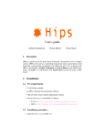
Figure 1.1: Nested dissection : Left, the graph before fill-in; right, the matrix with fill-in.
One fill-in edge will be created betwen two unknowns i and j if there is a path from i to j passing
only through vertices with number lower than min(i,j).
To save memory and computation time during decomposition, this fill-in has to be minimized. To
manage this several algorithms are used.
First, we use a nested dissection (fig. 1.1, p. 5) : we search in the graph for a separator S of
minimal size that cuts the graph into two parts of about the same size.
Then the separator nodes are indexed with the highest numbers available, so that no fill-in terms
will appear during decomposition between the unknowns of the two separated parts of the graph.
The algorithm is then repeated on each subgraph. This step also produces a dependency graph
used to distribute computations onto the processors.
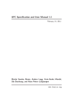
When the subgraph is smaller than a specified threshold, the Halo Approximate Minimum Degree
algorithm (fig. 1.2, p. 6) is used.
This algorithm further reduces the number of “fill-in” terms even more by assigning the smallest
available numbers to the nodes with lowest degree. Direct and foreign neighbors (halo) are
considered, in order not to neglect interactions with the whole graph.
An elimination tree can be constructed by using the following rule : there is an edge between i
andj if the first nonzero entry of column i is at row j.
This tree represents the dependancies between the computation steps. The wider and deeper it
is, the less the computation are dependent from each other.
The goal of the reordering step is to minimize “fill-in” and to reduce the dependancies between
computations.
This algorithm also compute a partition of the columns. This partition results from the fusion
of the separators and the sub-graphs reordered using the Halo Approximate Minimum Degree
algorithm.
5
original graph
5
halo
fill-in edge
4
2
1
3
Figure 1.2: Halo Approximate Minimum Degree.
1.3
Symbolic factorization
The symbolic factorization step computes the structure of the factorized matrix from the original
matrix A.
The factorization is done by blocks. This computation is cheap, its complexity depend on the
number of extra-diagonal blocs in the decomposed matrix.
1.4
Distribution and scheduling.
PaStiXuses static ordering by default. Computation is organized, in advance, for maximum
alignment with the parallel architecture being used.
The algorithm is composed of two steps.
The first step is the partitioning step. The largest blocks are cut into smaller pieces to be computed
by several processors. Full block parallel computation parallelism is used. It is applied on biggest
separators of the elimination tree, after the decomposition.
During this step, the elimination tree is traversed from the root to the leaves and for each block,
a set of processor candidates able to handle it is computed. This idea of “processor candidate”
is essential for the preservation of communication locality; this locality is obtain following the
elimination tree, because only the processors which compute a part of the subtree of a node would
be candidate for this node.
The second step is the distributing phase, each block will be associated to one of its candidates
wich will compute it.
To do so, the elimination tree is climbed up from the leaves to the root and, to distribute every
node of the tree on processors, the computation and communication time is computed for each
block. Thus, each block is allocated to the processor which will finish its processing first.
This step schedules computation and communication precisely; it needs an accurate calibration of
BLAS3 and communications operations on the destination architecture. The perf module contains
information about this calibration.
Thus, three levels of parallelism are used :
• Coarse grained parallelism, induced by independant computation between two subtrees of
one node. This parallelism is also called sparse induced parallelism,
6
• Medium grained parallelism, induced by dense blocks decomposition. This is a node level
parallelism, due to the possibility of cutting elimination tree nodes to distribute them onto
different processors,
• thin grained parallelism, obtained by using BLAS3 operations. This requires that the block
size be correctly choosen.
1.5
Factorization
The numeric solution of the problem computes a parallel Crout (LLt or LDLt ) or Cholesky (LU )
decomposition with a one-dimension column block distribution of the matriX.
Two type of algorithm exist, super-nodal, coming directly from column elimination algorithmn
rewritten by blocks, and multi-frontal.
Among super-nodals methods, the fan-in or left-looking method involves getting previous column
blocks modifications to compute next column blocks.
The contrary, the fan-out or right-looking method involves computing the current column block
and modifying next column blocks.
In PaStiX, the fan-in method, more efficient in parallel, has been implemented. This method
has the advantage of considerably reducing communication volume.
1.6
Solve
The solve step uses the up-down method. Since this computation is really cheap compared to
decomposition the decomposition distribution is kept.
1.7
Refinement
If the precision of the result of the Solve step is unsufficient, iterative refinement can be performed.
This section described the several iterative methods implemented in PaStiX.
1.7.1
GMRES
The GMRES algorithm used in PaStiX is based on work with Youssef Saad that can be found in
[Saa96].
1.7.2
Conjuguate gradiant
The conjugate gradient method is available with LLt and LDLt factorizations.
1.7.3
Simple iterative refinement
This method, described in algorithm 1 p.8, computes the difference bi between b and Ax and solves
the system Ax = bi . The solution xi are added to the initial solution, and the process repeated
|b−A×x|k
) is small enough.
until the relative error (M axk ( ||A||x|+|b||
k
This method is only available with LU factorization.
7
Algorithm 1 Static pivoting refinement algorithm
lerr ← 0;
f lag ← T RU E;
while f lag do
r ← b − A × x;
r0 ← |A||x| + |b|;
err ← maxi=0..n ( rr[i]
0 [i] );
if last err = 0 then
last err ← 3 × err;
rberror ← ||r||/||b||;
if (iter < iparm[IP ARM IT ERM AX] and
err > dparm[DP ARM EP SILON REF IN EM EN T ] and
err ≤ lerr
2 )
then
r0 ← x;
x ← solve(A × x = r);
r0 ← r0 + x;
last err ← err;
iter ← iter + 1;
else
f lag ← F ALSE;
1.8
Out-of-core
An experimental out-of-core version of PaStiX has been written.
Directions for compiling this version are given in section 2.3.7.
For the moment, only multi-threaded version is supported, the hybrid “MPI+threads” version is
likely to lead to unresolved deadlocks.
The disk inputs and outputs are managed by a dedicated thread. This thread will prefetch column
blocks and communication buffers so that computing threads will be abble to use them.
As the whole computation as been predicted, the out-of-core thread will follow the scheduled
computation and prefetch needed column blocks. It will also save them, depending on their next
acces, if the memory limit is reached.
The prefetch algorithm is not dependant of the number of computation threads, it will follow the
computation algorithm as if there was only one thread.
8
Chapter 2
Compilation of PaStiX
This chapter will present how to quickly compile PaStiX and the different compilation options
that can be used with PaStiX.
2.1
2.1.1
Quick compilation of PaStiX
Pre-requirement
To compile PaStiX, a BLAS library is required.
To compile PaStiX, it is advise to get first Scotch or PT-Scotch ordering library (https:
//gforge.inria.fr/projects/scotch/).
However, it is possible to compile PaStiX with Metis or without any ordering (using user ordering), or even both. Metis and Scotch or PT-Scotch.
To be able to use threads in PaStiX, the pthread library is required.
For a MPI version of PaStiX, a MPI library is obviously needed.
2.1.2
compilation
To compile PaStiX, select in src/config/ the compilation file corresponding to your architecture,
and copy it to src/config.in.
You can edit this file to select good libraries and compilation options.
Then you can run make expor install to compile PaStiX library.
This compilation will produce PaStiX library, named libpastix.a; PaStiX C header, named
pastix.h; a Fortran header named pastix fortran.h (use it with #include) and a script,
pastix-conf that will descripes how PaStiX has been compiled (options, flags...). This script is
used to build the Makefile in example/src.
Another library is produced to use Murge interface : libpastix murge.a, which works with the
C header murge.h and the Fortran header murge.inc (a true Fortran include).
9
2.2
Makefile keywords
make help :
make all :
print this help;
build PaStiX library;
make debug :
build PaStiX library in debug mode;
make drivers :
build matrix drivers library;
make debug drivers :
make examples :
build matrix drivers library in debug mode;
build examples (will run ’make all’ and ’make drivers’ if needed);
make murge : build murge examples (only available in distributed mode -DDISTRIBUTED, will
run ’make all’ and ’make drivers’ if needed);
make python :
make clean :
Build python wrapper and run src/simple/pastix python.py;
remove all binaries and objects directories;
make cleanall :
2.3
2.3.1
remove all binaries, objects and dependencies directories
Compilation flags
Integer types
PaStiX can be used with different integer types. User can choose the integer type by setting
compilation flags.
The flag -DINTSIZE32 will set PaStiX integers to 32 bits integers.
The flag -DINTSIZE64 will set PaStiX integers to 64 bits integers.
If you are using Murge interface, you can also set -DINTSSIZE64 to set Murge’s INTS integers to
64 bits integers. This is not advised, INTS should be 32 bit integers.
2.3.2
Coefficients
Coefficients can be defined to several types:
real : using no flag,
double : using flag -DPREC DOUBLE,
complex : using flag -DTYPE COMPLEX,
double complex : using both -DTYPE COMPLEX and -DPREC DOUBLE flags.
2.3.3
MPI and Threads
PaStiX default version uses threads and MPI.
The expected way of running PaStiX is with one MPI process by node of the machine and one
thread for each core.
It is also possible to deactivate MPI using -DFORCE NOMPI and threads using -DFORCE NOSMP. User
only has to uncomment the corresponding lines of his config.in file.
10
PaStiX also proposes the possibility to use one thread to handle communications reception. It
can give better results if the MPI librairy does not handle correctly the communication progress.
This option is activated using -DTHREAD COMM.
If the MPI implementation does not handle MPI THREAD MULTIPLE a funneled version of PaStiX
is also proposed. This version, available through -DTHREAD MULTIPLE, can affect the solver performances.
An other option of PaStiX is provided to suppress usage of MPI types in PaStiX if the MPI implementation doesn’t handle it well. This option is available with the compilation flag -DNO MPI TYPE.
The default thread library used by PaStiX is the POSIX one.
The Marcel library, from the INRIA team Runtime can also be used. Through marcel, the
Bubble scheduling framework can also be used defining the option -DPASTIX USE BUBBLE.
All this options can be set in the Marcel section of the config.in file.
2.3.4
Ordering
The graph partitioning can be done in PaStiX using Scotch, PT-Scotch or Metis. It can
also be computed by user and given to PaStiX through the permutation arrays parameters. To
activate the possibility of using Scotch in PaStiX (default) uncomment the corresponding lines
of the config.in.
In the same way, to use Metis, uncomment the corresponding lines of the config.in file.
Scotch and Metis can be used together, alone, or can be unused.
PT-Scotch is required when the -DDISTRIBUTED flag has been set, that is to say, when compiling
with the distributed interface.
When using centralised interface with PT-Scotch, the ordering will be performed with Scotch
functions.
2.3.5
NUMA aware library
To be more efficient on NUMA machines, the allocation of the matrix coefficient is can be performed
on each thread.
The default compilation flag -DNUMA ALLOC will activate this “per thread” allocation.
2.3.6
Statistics
Memory usage
The compilation flag MEMORY USAGE can be used to display memory usage at deferent steps of
PaStiX run.
The information also appear in double parameter output array, at index DPARM MEM MAX. The value
is given in octets.
2.3.7
Out-of-core
It is possible to experiment an out-of-core version of PaStiX.
To compile PaStiX with Out Of Core, compile it with -DOOC.
11
2.3.8
Python wrapper
A simple python wrapper can be built to use PaStiX from python.
This wrapper uses SWIG (Simplified Wrapper and Interface Generator - www.swig.org).
To build the python interface, user needs to use dynamic (or at least built with -fPIC) libraries
(for BLAS, MPI and Scotch.
It is also necessary to uncomment the Python part of the config.in file and set paths correctly for
MPI4PY DIR, MPI4PY INC and MPI4PY LIBDIR.
Then you just have to run make python to build the interface and test it with examples/src/pastix python.py.
12
Chapter 3
PaStiX options
PaStiX can be called step by step or in one unique call.
User can refer to PaStiX step-by-step and simple examples.
The folowing section will describe each steps and options that can be used to tune the computation.
3.1
Global parameters
This section present list of parameters used in severall PaStiX steps.
3.1.1
Verbosity level
IPARM VERBOSE : used to set verbosity level. Can be set to 3 values :
API VERBOSE NOT : No display at all,
API VERBOSE NO : Few displays,
API VERBOSE YES : Maximum verbosity level.
3.1.2
Indicating the steps to execute
IPARM START TASK : indicates the first step to execute (cf. quick reference card).
Should be set before each call.
It is modified during PaStiX calls, at the end of one call it is equal to the last step performed
(should be IPARM END TASK.
IPARM END TASK : indicates the last step to execute (cf. quick reference card).
Should be set before each call.
NB : Setting IPARM MODIFY PARAMETER to API NO will make PaStiX initialize integer and floating
point parameters. After that operation, PaStiX will automaticaly return, without taking into
acount IPARM START TASK nor IPARM END TASK.
3.1.3
Symmetry
IPARM FACTORISATION : Gives the factorisation type.
It can be API FACT LU, API FACT LDLT or API FACT LLT.
13
It has to be set from ordering step to refinement step to the same value.
With non symmetric matrix, only LU factorisation is possible.
IPARM SYM : Indicates if the matrix is symmetric or not.
With symmetric matrix, only the inferior triangular part has to be given.
3.1.4
Threads
To save memory inside a SMP node users can use threads inside each node.
Each thread will allocate the part of the matrix he will work mostly on but all threads will share
the matrix local to the SMP node.
IPARM THREAD NBR : Number of computing threads per MPI process,
IPARM BINDTHRD : can be set to the mode used to bind threads on processors :
API BIND NO : do not bind threads on processors,
n
API BIND AUTO : default binding mode (thread are binded cyclicaly (thread n to proc b procnbr
c),
API BIND TAB : Use vector given by pastix setBind (?? p.??).
This section describes which steps are affected by which options.
3.1.5
Matrix descriprion
PaStiX solver can handle different type of matrices.
User can describe the matrix using several parameters :
IPARM DOF NBR : indicate the number of degree of freedom by edge of the graph. The default
value is one.
IPARM SYM : indicate if the matrix is symmetric or not. This parameters can be set to two values :
API SYM YES : If the matrix is symmetric.
API SYM NO : If the matrix is not symmetric.
If user is not sure that the matrix will fit PaStiX and Scotch requirements, the parameters
IPARM MATRIX VERIFICATION can be set to API YES.
With distributed interface, to prevent PaStiX from checking that the matrix has been correctly
distributed after distribution computation, IPARM CSCD CORRECT can be set to API YES.
3.2
3.2.1
Initialisation
Description
This steps initializes the pastix data structure for next PaStiX calls.
It can also initialize integer and double parameters values (see quick reference card for default
values).
It has to be called first.
14
3.2.2
Parameters
To call this step you have to set IPARM START TASK to API TASK INIT.
When this step is called, IPARM MODIFY PARAMETER should be set to API NO. This will make PaStiX
set all integer and double parameters.
If IPARM MODIFY PARAMETER is set to API NO, pastix will automaticaly return after initialisation,
whatever IPARM END TASK is set to.
The user CSC matrix can be checked during this step. To perform matrix verification, IPARM MATRIX VERIFICATION
has to be set to API YES.
This will correct numbering if the CSC is in C numbering, sort the CSC and check if the graph of
the matrix is symmetric (only is the matrix is non-symmetric (depending on iparm[IPARM SYM]
value).
It is also possible to use pastix checkMatrix function (4.4.3 p.29) to perform this checking operations and also correct the graph symmetry .
3.3
Ordering
3.3.1
Description
The ordering step will reorder the unknowns of the matrix to minimize fill-in during factorisation.
This step is description in 1.2
3.3.2
Parameters
To call ordering step, IPARM START TASK has to be set to API TASK ORDERING or previous task and
IPARM END TASK must be greater or equal to ordering one.
Ordering can be computed with Scotch or Metis.
To enable Metis, user has to uncomment the corresponding part of the config.in file. To select
the ordering software, user may set IPARM ORDERING to :
• API ORDER SCOTCH : use Scotch for the ordering (default)
• API ORDER METIS : use Metis for the ordering.
To have a finer control on the ordering software, user can set IPARM DEFAULT ORDERING to API YES
and modify those parameters:
• when using Scotch :
IPARM ORDERING SWITCH LEVEL : ordering switch level (see Scotch User’s Guide),
IPARM ORDERING CMIN : ordering cmin parameter (see Scotch User’s Guide),
IPARM ORDERING CMAX : ordering cmax parameter (see Scotch User’s Guide),
IPARM ORDERING FRAT : ordering frat parameter (×100) (see Scotch User’s Guide).
• when using Metis :
IPARM ORDERING SWITCH LEVEL : Metis ctype option,
IPARM ORDERING CMIN : Metis itype option,
IPARM ORDERING CMAX : Metis rtype option,
IPARM ORDERING FRAT : Metis dbglvl option,
15
IPARM STATIC PIVOTING : Metis oflags option,
IPARM METIS PFACTOR : Metis pfactor option,
IPARM NNZERO : Metis nseps option.
3.4
3.4.1
Symbolic factorisation
Description
This step is the symbolic factorisation step described in 1.3.
3.4.2
Parameters
If user didn’t called ordering step with Scotch, IPARM LEVEL OF FILL has to be set to -1 to use
KASS algorithm.
If PaStiX was compiled with -DMETIS, this parameter will be forced to -1.
If PaStiX runs KASS algorithm, IPARM AMALGAMATION LEVEL will be take into account.
KASS will merge supernodes untill fill reaches IPARM AMALGAMATION LEVEL.
3.5
3.5.1
Analyse
Description
During this step, PaStiX will simulate factorization and decide where to assign each part of the
matrix.
More details can be read in 1.4
3.5.2
Parameters
IPARM MIN BLOCKSIZE : Minimum size of the column blocks computed in blend;
IPARM MAX BLOCKSIZE : Maximum size of the column blocks computed in blend.
3.5.3
Output
DPARM ANALYZE TIME : time to compute analyze step,
DPARM PRED FACT TIME : predicted factorization time (with IBM PWR5 ESSL).
3.6
3.6.1
Numerical factorisation
Description
Numerical factorisation (1.5)of the given matrix.
Can be LU , LLt , or LDLt factorisation.
16
3.6.2
Parameters
DPARM EPSILON MAGN CTRL : value which will be used for static pivoting. Diagonal values smaller
than it will be replaced by it.
3.6.3
Ouputs
After factorisation, IPARM STATIC PIVOTING : will be set to the number of static pivoting performed.
A static pivoting is performed when a diagonal value is smaller than DPARM EPSILON MAGN CTRL.
IPARM ALLOCATED TERMS : Number of non zeros allocated in the final matrix,
DPARM FACT TIME : contains the time spent computing factorisation step in seconds, in real time,
not cpu time,
DPARM SOLV FLOPS : contains the number of operation per second during factorisation step.
3.7
Solve
3.7.1
Description
This step, described in 1.6, will compute the solution of the system.
3.7.2
Parameters
IPARM RHS MAKING : way of obtaining the right-hand-side member :
API RHS B : get right-hand-side member from user,
API RHS 1 : construct right-hand-side member such as the solution X is defined by : ∀i, Xi =
1,
API RHS I : construct right-hand-side member such as the solution X is defined by : ∀i, Xi =
i,
3.7.3
Ouputs
DPARM SOLV TIME : contains the time spent computing solve step, in second, in real time, not cpu
time,
DPARM SOLV FLOPS : contains the number of operation per second during solving step.
3.8
Refinement
3.8.1
Description
After solving step, it is possible to call for refinement is the precision of the solution is not sufficient.
17
3.8.2
Parameters
To call for refinement, IPARM START TASK must be lower than API TASK REFINEMENT and IPARM END TASK
must be greater than API TASK REFINEMENT.
A list of parameters can be used to setup refinement step :
IPARM ITERMAX : Maximum number of iteration in refinement step,
IPARM REFINEMENT : Type of refinement :
API RAF GMRES : GMRES algorithm,
API RAF PIVOT : a simple iterative algorithm, can only be used with LLt or LDLt factorization (the corresponding iparm must be correctly set),
API RAF GRAD : conjugate gradient algorithm, can only be used with LU factorization (the
corresponding iparm must be correctly set).
IPARM GMRES IM : syze of the Krylov space used in GMRES,
DPARM EPSILON REFINEMENT : Desired solution precision.
3.8.3
Output
After refinement, IPARM NBITER will be set to the number of iteration performed during refinement.
The value DPARM RELATIVE ERROR will be the error between AX and B. It should be smaller than
DPARM EPSILON REFINEMENT.
DPARM RAFF TIME contains the time spent computing solve step, in second.
3.9
Clean
This step simply free all memory used by PaStiX.
18
Chapter 4
PaStiX functions
The PaStiX library provides several functions to setup and run PaStiX decomposition steps.
Two different ways of using PaStiX exist, it can be called with a sequential matrix in input, or
with a distributed matrix.
The sequential library is composed of a main function pastix. The ditributed PaStiX library
has to interfaces. The original one is based on the sequential one, it is composed of few auxiliary
functions and one main function which, depending on parameters, will run all steps.
The third one is an interface which has been haded to match with HIPS and MUMPS interfaces.
4.1
Original sequential interface
The original interface is composed of one main function. Few auxiliary functions also permit to
check that the user matrix will fit with PaStiX matrix format.
4.1.1
The main function
The main function of the original sequential interface is the pastix function (Fig. 4.1, p.19).
It is used to run separatly or in one call all PaStiX decomposition steps.
A fortran interface to this function is also available in PaStiX library (Fig. 4.2, p.20).
In this centralised interface to PaStiX, all paramteters should be equal on all MPI processors.
The first parameter, pastix data is the address of a structure used to store data between pastix
calls. It has to be set to NULL (0 in Fortran) before first call. This parameter is modified by
PaStiX and should be untuched until the end of the program execution.
#include “pastix.h”
void pastix ( pastix
pastix
pastix
pastix
pastix
pastix
data t ** pastix data,
int t
n,
int t * row,
int t * perm,
float t * b,
int t * iparm,
MPI Comm
pastix int t
pastix float t
pastix int t
pastix int t
double
pastix comm,
* colptr,
* avals,
* invp,
rhs,
* dparm );
Figure 4.1: PaStiX main function prototype
19
#include “pastix fortran.h”
pastix data ptr t
integer
pastix int t
pastix float t
pastix int t
real*8
call pastix fortran
:: pastix data
:: pastix comm
:: n, rhs, ia(n), ja(nnz)
:: avals(nnz), b(n)
:: perm(n), invp(n), iparm(64)
:: dparm(64)
( pastix data, pastix comm, n, ia, ja, avals,
perm, invp, b, rhs, iparm, dparm )
Figure 4.2: PaStiX main function fortran interface

1
0

2

0
0
0
3
0
4
0
0
0
5
6
0
0
0
0
7
0

0
0

0

0
8
colptr
row
avals
=
=
=
{1, 3, 5, 7, 8, 9}
{1, 3, 2, 4, 3, 4, 4, 5}
{1, 2, 3, 4, 5, 6, 7, 8}
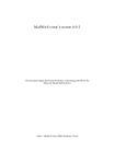
Figure 4.3: CSC matrix example
pastix comm is the MPI communicator used in PaStiX.
n, colptr, row and avals is the matrix to factorize, ni CSC representation (Fig. 4.3 p.20).
n is the size of the matrix, colptr is an array of n + 1 pastix int t. It contains index of first
elements of each column in row, the row of each non null element, and avals, the value of each
non null element.
perm (resp. invp) is the permutation (resp. reverse permutation) tabular. It is an array of n
pastix int t and must be allocated by user. It is set during ordering step but can also be set by
user.
b is an array of n × rhs pastix float t. It correspond to the right-hand-side member(s) and will
contain the solution(s) at the end of computation.
Right-hand-side members are contiguous in this array.
rhs is the number of right-hand-side members. Only one is currently accepted by PaStiX.
iparm is the integer parameters array, of IPARM SIZE pastix int t.
dparm is the floating parameters array, of DPARM SIZE double.
The only parameters that can be modified by this function are pastix data, iparm and dparm.
4.2
Original Distributed Matrix Interface
A new interface was added to run PaStiX using ditributed data (Fig. 4.6 p.22 and Fig. 4.7 p.22).
The Data is given distributed by columns.
The original CSC is replaced by a distributed CSC (Fig. 4.4, p.21).
4.2.1
A distributed CSC
A distributed CSC is a CSC with a given list of columns. An additionnal array give the global
number of each local column.
20
dCSC

P1
1

0

2

0
0
On processor one :
colptr
= {1, 3, 5, 6}
row
= {1, 3, 3, 4, 5}
avals
= {1, 2, 5, 6, 8}
loc2glb = {1, 3, 5}
On processor two :
colptr
= {1, 3, 4}
row
= {2, 4, 4}
avals
= {3, 4, 7}
loc2glb = {2, 4}
matrix example :

P 2 P1 P2 P1
0
0
0
0

3
0
0
0

0
5
0
0

4
6
7
0
0
0
0
8
Figure 4.4: A distributed CSC
4.2.2
Usage of the distributed interface
A good usage of the distributed interface would follow this steps (Fig. 4.5 p.22) :
1. provide the graph to PaStiX in user’s distribution to perform analyze steps;
2. get the solver distribution from PaStiX.
3. provide the matrice and right-hand-side in PaStiX distribution to avoid redistribution inside
the solver and perform factorization and solving steps.
An example of this utilisation of the distributed interface can be found in src/example/src/simple dist.c.
4.2.3
The distributed interface prototype
The distributed interface prototype is similar to the centralised one, only a loc2glob array is added
to it.
4.3
4.3.1
Murge : Uniformized Distributed Matrix Interface
Description
This interface was added to PaStiX to simplify the utilisation of multiple solvers, HIPS and
PaStiX in a first step, other Murge compliant solvers later.
It is composed of a large number of function but it is less flexible than the original one.
Using this interface, you can change between solvers with only few modifications. You just have
to set specific solvers option.
This new interface has been created trying to simplify user work, thinkinig about his needs.
The graph is simply built in order to compute the distribution of the problem. Then the matrix
is filled taking account or ignoring the solver distribution. After that the right-hand-side id given
and the solution is computed.
More information about this new interface can be found at http://murge.gforge.inria.fr/.
21
/∗ B u i l d t h e CSCd graph with e x t e r n a l s o f t w a r e d i s t r i b u t i o n ∗/
iparm [ IPARM START TASK ]
iparm [ IPARM END TASK ]
= API TASK ORDERING ;
= API TASK BLEND ;
d p a s t i x (& p a s t i x d a t a , MPI COMM WORLD,
n c o l , c o l p t r , rows , NULL, l o c 2 g l o b ,
perm , NULL, NULL, 1 , iparm , dparm ) ;
n c o l 2 = p a s t i x g e t L o c a l N o d e N b r (& p a s t i x d a t a ) ;
i f (NULL == ( l o c 2 g l o b 2 = m a l l o c ( n c o l 2 ∗ s i z e o f ( p a s t i x i n t t ) ) ) )
{
f p r i n t f ( s t d e r r , ” Malloc e r r o r \n ” ) ;
r e t u r n EXIT FAILURE ;
}
p a s t i x g e t L o c a l N o d e L s t (& p a s t i x d a t a , l o c 2 g l o b 2 ) ;
. . . /∗ B u i l d i n g t h e matrix f o l l o w i n g PaStiX d i s t r i b u t i o n ∗/
iparm [ IPARM START TASK ]
iparm [ IPARM END TASK ]
= API TASK NUMFACT ;
= API TASK CLEAN ;
d p a s t i x (& p a s t i x d a t a , MPI COMM WORLD,
n c o l 2 , c o l p t r 2 , rows2 , v a l u e s 2 , l o c 2 g l o b 2 ,
perm , invp , rhs2 , 1 , iparm , dparm ) ;
Figure 4.5: Using distributed interface
#include “pastix.h”
void dpastix ( pastix
pastix
pastix
pastix
pastix
pastix
pastix
data t ** pastix data,
int t
n,
int t * row,
int t * loc2glb,
int t * perm,
float t * b,
int t * iparm,
MPI Comm
pastix comm,
pastix int t * colptr,
pastix float t * avals,
pastix int t
pastix int t
double
* invp,
rhs,
* dparm );
Figure 4.6: Distributed C interface
#include “pastix fortran.h”
pastix data ptr t
integer
pastix int t
pastix float t
pastix int t
real*8
call dpastix fortran
:: pastix data
:: pastix comm
:: n, rhs, ia(n+1), ja(nnz)
:: avals(nnz), b(n)
:: loc2glb(n), perm(n), invp(n), iparm(64)
:: dparm(64)
( pastix data, pastix comm, n, ia, ja, avals,
loc2glob perm, invp, b, rhs, iparm, dparm )
Figure 4.7: Distributed fortran interface
22
4.3.2
Additional specific functions for PaStiX
Few auxilary functions were added in the PaStiX implementation of this interface. They are not
essential, Murge can be used without this functions.
MURGE Analyze
INTS MURGE Analyze ( INTS id );
SUBROUTINE MURGE ANALYZE ( ID, IERROR)
INTS, INTENT(IN)
:: ID
INTS, INTENT(OUT)
:: IERROR
END SUBROUTINE MURGE ANALYZE
Parameters :
id : Solver instance identification number.
Perform matrix analyze:
• Compute a new ordering of the unknows
• Compute the symbolic factorisation of the matrix
• Distribute column blocks and computation on processors
This function is not needed to use Murge interface, it only forces analyze step when user wants.
If this function is not used, analyze step will be performed when getting new distribution from
MURGE, or filling the matrix.
MURGE Factorize
INTS MURGE Factorize ( INTS id);
SUBROUTINE MURGE FACTORIZE ( ID, IERROR)
INTS, INTENT(IN)
:: ID
INTS, INTENT(OUT)
:: IERROR
END SUBROUTINE MURGE FACTORIZE
Parameters :
id : Solver instance identification number.
Perform matrix factorization.
This function is not needed to use Murge interface, it only forces factorization when user wants.
If this function is not used, factorization will be performed with solve, when getting solution from
MURGE.
MURGE SetOrdering
INTS MURGE SetOrdering ( INTS id, INTS * permutation);
23
SUBROUTINE MURGE SETORDERING ( ID, PERMUTATION, IERROR)
INTS, INTENT(IN)
:: ID
INTS, INTENT(IN), DIMENSION(0)
:: PERMUTATION
INTS, INTENT(OUT)
:: IERROR
END SUBROUTINE MURGE SETORDERING
Parameters :
id
: Solver instance identification number.
permutation : Permutation to set internal computation ordering
Set permutation for PaStiX internal ordering.
The permutation array can be unallocated after the function is called.
MURGE ForceNoFacto
INTS MURGE ForceNoFacto ( INTS id);
SUBROUTINE MURGE FORCENOFACTO ( ID, IERROR)
INTS, INTENT(IN)
:: ID
INTS, INTENT(OUT)
:: IERROR
END SUBROUTINE MURGE FORCENOFACTO
Parameters :
id : Solver instance identification number.
Prevent Murge from running factorisation even if matrix has changed.
If an assembly is performed, next solve will trigger factorization except if this function is called
between assembling the matrix and getting the solution.
MURGE GetLocalProduct
INTS MURGE GetLocalProduct ( INTS id, COEF * x);
SUBROUTINE MURGE GETLOCALPRODUCT ( ID, x, IERROR)
INTS, INTENT(IN)
:: ID
COEF, INTENT(OUT), DIMENSION(0)
:: X
INTS, INTENT(OUT)
:: IERROR
END SUBROUTINE MURGE GETLOCALPRODUCT
Parameters :
id : Solver instance identification number.
x : Array in which the local part of the product will be stored.
Perform the product A × x and returns its local part.
The vector must have been given through MURGE SetLocalRHS or MURGE SetGlobalRHS.
MURGE GetGlobalProduct
INTS MURGE GetGlobalProduct ( INTS id, COEF * x);
24
SUBROUTINE MURGE GETGLOBALPRODUCT ( ID, x, IERROR)
INTS, INTENT(IN)
:: ID
COEF, INTENT(OUT), DIMENSION(0)
:: X
INTS, INTENT(OUT)
:: IERROR
END SUBROUTINE MURGE GETGLOBALPRODUCT
Parameters :
id : Solver instance identification number.
x : Array in which the product will be stored.
Perform the product A × x and returns it globaly.
The vector must have been given through MURGE SetLocalRHS or MURGE SetGlobalRHS.
MURGE SetLocalNodeList
INTS MURGE SetLocalNodeList ( INTS id,
INTS nodenbr
(
INTS * nodelist);
SUBROUTINE MURGE SETLOCALNODELIST ( ID, nodenbr, nodelist, IERROR)
INTS, INTENT(IN)
:: ID
INTS, INTENT(IN)
:: nodenbr
INTS, INTENT(IN), DIMENSION(0)
:: nodelist
INTS, INTENT(OUT)
:: IERROR
END SUBROUTINE MURGE SETLOCALNODELIST
Parameters :
id
: Solver instance identification number.
nodenbr : Number of local nodes.
nodelist : Array containing global indexes of local nodes.
Set the distribution of the solver, preventing the solver from computing its own.
NEEDS TO BE CHECKED !
MURGE AssemblySetSequence
INTS MURGE AssemblySetSequence ( INTS id ,
INTS * ROWs,
INTS op,
INTS mode,
INTS * id seq);
INTL coefnbr,
INTS * COLs,
INTS op2,
INTS nodes,
SUBROUTINE MURGE ASSEMBLYSETSEQUENCE ( ID, coefnbr, ROWs, COLs,
op, op2, mode, nodes,
id seq, IERROR)
INTS, INTENT(IN)
:: ID
INTL, INTENT(IN)
:: coefnbr
INTS, INTENT(IN), DIMENSION(0)
:: ROWs, COLs
INTS, INTENT(IN)
:: op, op2, mode, nodes
INTS, INTENT(OUT)
:: id seq
INTS, INTENT(OUT)
:: IERROR
END SUBROUTINE MURGE ASSEMBLYSETSEQUENCE
25
Parameters :
id
:
coefnbr :
ROWs
:
COLs
:
op
:
op2
mode
nodes
id seq
Solver instance identification number.
Number of local entries in the sequence.
List of rows of the sequence.
List of columns of the sequence.
Operation to perform for coefficient which appear several tim (see
MURGE ASSEMBLY OP).
: Operation to perform when a coefficient is set by two different processors (see MURGE ASSEMBLY OP).
: Indicates if user ensure he will respect solvers distribution (see
MURGE ASSEMBLY MODE).
: Indicate if entries are given one by one or by node :
0 : entries are entered value by value,
1 : entries are entries node by node.
: Sequence ID.
Create a sequence of entries to build a matrix and store it for being reused.
MURGE AssemblyUseSequence
INTS MURGE AssemblyUseSequence ( INTS
id ,
INTS id seq,
COEF * values);
SUBROUTINE MURGE ASSEMBLYUSESEQUENCE ( ID, id seq, values, IERROR)
INTS, INTENT(IN)
:: ID
INTS, INTENT(IN)
:: id seq
COEF, INTENT(IN), DIMENSION(0)
:: values
INTS, INTENT(OUT)
:: IERROR
END SUBROUTINE MURGE ASSEMBLYUSESEQUENCE
Parameters
id
:
id seq :
values :
:
Solver instance identification number.
Sequence ID.
Values to insert in the matrix.
Assembly the matrix using a stored sequence.
MURGE AssemblyDeleteSequence
INTS MURGE AssemblyDeleteSequence ( INTS id , INTS id seq);
SUBROUTINE MURGE ASSEMBLYDELETESEQUENCE ( ID, id seq, IERROR)
INTS, INTENT(IN)
:: ID
INTS, INTENT(IN)
:: id seq
INTS, INTENT(OUT)
:: IERROR
END SUBROUTINE MURGE ASSEMBLYDELETESEQUENCE
Parameters :
id
: Solver instance identification number.
id seq : Sequence ID.
Destroy an assembly sequence.
26
4.4
4.4.1
Auxiliary PaStiX functions
Distributed mode dedicated functions
Getting local nodes number
pastix int t pastix getLocalNodeNbr ( pastix data t ** pastix data );
SUBROUTINE PASTIX FORTRAN GETLOCALNODENBR ( PASTIX DATA,
NODENBR)
pastix data ptr t, INTENT(INOUT) :: PASTIX DATA
INTS, INTENT(OUT)
:: NODENBR
END SUBROUTINE PASTIX FORTRAN GETLOCALNODENBR
Parameters :
pastix data : Area used to store information between calls.
Return the node number in the new distribution computed by the analyze step
(Analyse step must have already been executed).
Getting local nodes list
int pastix getLocalNodeLst ( pastix data t ** pastix data,
pastix int t * nodelst );
SUBROUTINE PASTIX FORTRAN GETLOCALNODELST ( PASTIX DATA,
NODELST,
IERROR)
:: PASTIX DATA
pastix data ptr t, INTENT(INOUT)
INTS, INTENT(OUT), DIMENSION(0)
:: NODELST
INTS, INTENT(OUT)
:: IERR
END SUBROUTINE PASTIX FORTRAN GETLOCALNODELST
Parameters :
pastix data : Area used to store information between calls.
nodelst
: Array to receive the list of local nodes.
Fill nodelst with the list of local nodes
(nodelst must be at least nodenbr*sizeof(pastix int t), where nodenbr is obtained from
pastix getLocalNodeNbr).
Getting local unknowns number
pastix int t pastix getLocalUnknownNbr ( pastix data t ** pastix data);
SUBROUTINE PASTIX FORTRAN GETLOCALUNKNOWNNBR ( PASTIX DATA,
UNKNOWNNBR)
pastix data ptr t, INTENT(INOUT) :: PASTIX DATA
INTS, INTENT(OUT)
:: UNKNOWNNBR
END SUBROUTINE PASTIX FORTRAN GETLOCALUNKNOWNNBR
27
Parameters :
pastix data : Area used to store information between calls.
Return the number of unknowns in the new distribution computed by the preprocessing.
Needs the preprocessing to be runned with pastix data before.
Getting local unknowns list
int pastix getLocalUnknownLst ( pastix data t ** pastix data,
pastix int t * unknownlst );
SUBROUTINE PASTIX FORTRAN GETLOCALUNKNOWNLST ( PASTIX DATA,
UNKNOWNLST,
IERROR)
pastix data ptr t, INTENT(INOUT)
:: PASTIX DATA
INTS, INTENT(OUT), DIMENSION(0)
:: UNKNOWNLST
INTS, INTENT(OUT)
:: IERR
END SUBROUTINE PASTIX FORTRAN GETLOCALUNKNOWNLST
Parameters :
pastix data : Area used to store information between calls.
nodelst
: An array where to write the list of local nodes/columns.
Fill in unknownlst with the list of local unknowns/column.
Needs unknownlst to be allocated with unknownnbr*sizeof(pastix int t), where unknownnbr
has been computed by pastix getLocalUnknownNbr.
4.4.2
Binding thread
void pastix setBind ( pastix data t ** pastix data, int
int
* bindtab );
thrdnbr,
SUBROUTINE PASTIX FORTRAN SETBINDTAB ( PASTIX DATA,
THRDNBR,
BINDTAB)
pastix data ptr t, INTENT(INOUT)
:: PASTIX DATA
INTS, INTENT(OUT)
:: THRDNBR
INTS, INTENT(OUT), DIMENSION(0)
:: BINDTAB
END SUBROUTINE PASTIX FORTRAN SETBINDTAB
Parameters :
pastix data : Area used to store information between calls.
thrdnbr
: Number of threads (== length of bindtab).
bindtab
: List of processors for threads to be binded on.
Assign threads to processors.
Thread number i (starting with 0 in C and 1 in Fortran) will be binded to the core bindtab[i]
28
4.4.3
Working on CSC or CSCD
Checking and correcting the CSC or CSCD matrix
void pastix checkMatrix ( MPI Comm
pastix comm,
int
flagsym,
n,
pastix int t
pastix int t ** row,
pastix int t ** loc2glob );
int
verb,
int
flagcor,
pastix int t ** colptr,
pastix float t ** avals,
int
dof
SUBROUTINE PASTIX FORTRAN CHECKMATRIX ( DATA CHECK
PASTIX COMM,
VERB,
FLAGSYM,
FLAGCOR,
N,
COLPTR,
ROW,
AVALS,
LOC2GLOB)
pastix data ptr t, INTENT(OUT)
:: DATA CHECK
MPI COMM, INTENT(IN)
:: PASTIX COMM
INTEGER, INTENT(IN)
:: VERB
INTEGER, INTENT(IN)
:: FLAGSYM
INTEGER, INTENT(IN)
:: FLAGCOR
pastix int t, INTENT(IN)
:: N
pastix int t, INTENT(IN), DIMENSION(0)
:: COLPTR
pastix int t, INTENT(IN), DIMENSION(0)
:: ROW
pastix int t, INTENT(IN), DIMENSION(0)
:: AVALS
:: LOC2GLOB
pastix int t, INTENT(IN), DIMENSION(0)
END SUBROUTINE PASTIX FORTRAN CHECKMATRIX
SUBROUTINE PASTIX FORTRAN CHECKMATRIX END ( DATA CHECK
VERB,
ROW,
AVALS)
pastix data ptr t, INTENT(IN)
:: DATA CHECK
INTEGER, INTENT(IN)
:: VERB
pastix int t, INTENT(IN), DIMENSION(0)
:: ROW
pastix int t, INTENT(IN), DIMENSION(0)
:: AVALS
END SUBROUTINE PASTIX FORTRAN CHECKMATRIX END
Parameters :
:
pastix comm
verb
:
flagsym
:
flagcor
:
n
:
colptr, row, avals :
loc2glb
:
PaStiX MPI communicator.
Verbose mode (see Verbose modes).
Indicates if the matrix is symmetric (see Symmetric modes).
Indicates if the matrix can be reallocated (see Boolean modes).
Matrix dimension.
Matrix in CSC format.
Local to global column number correspondance.
Check and correct the user matrix in CSC format :
• Renumbers in Fortran numerotation (base 1) if needed (base 0)
• Can scale the matrix if compiled with -DMC64 -DSCALING (untested)
• Checks the symetry of the graph in non symmetric mode. With non distributed matrices,
with f lagcor == AP I Y ES, tries to correct the matrix.
29
• sort the CSC.
In fortran, with correction enable, CSC array can be reallocated.
PaStiX works on a copy of the CSC and stores it internaly if the number of entries changed.
If the number of entries changed (colptr[n] − 1), user as to reallocate rows and avals and then call
PASTIX FORTRAN CHECKMATRIX END().
Checking the symetry of a CSCD
n,
pastix int t * ia,
int cscd checksym ( pastix int t
pastix int t * ja,
pastix int t * l2g,
comm );
MPI Comm
Parameters :
n : Number of local columns.
ia : Starting index of each column in ja.
ja : Row of each element.
l2g : Global column numbers of local columns.
Check the graph symmetry.
Correcting the symetry of a CSCD
int cscd symgraph ( pastix
pastix
pastix
pastix
pastix
int
int
int
int
int
t
t
t
t
t
*
*
**
*
n,
ja,
newn,
newja,
l2g,
pastix int t
pastix float t
pastix int t
pastix float t
MPI Comm
*
*
**
**
ia,
a,
newia,
newa,
comm,
Parameters :
n
: Number of local columns.
ia
: Starting index of each column in ja and a.
ja
: Row of each element.
a
: Value of each element.
newn : New number of local columns.
newia : Starting index of each columns in newja and newa.
newja : Row of each element.
newa : Values of each element.
l2g : Global number of each local column.
comm : MPI communicator.
Symmetrize the graph.
30
Adding a CSCD into an other one
int cscd addlocal ( pastix int t
pastix int t
pastix int t
pastix int t
pastix float t
pastix int t
pastix int t
CSCD OPERATIONS t
Parameters :
n
ia
ja
a
l2g
addn
addia
addja
adda
addl2g
newn
newia
newja
newa
malloc flag
OP
:
:
:
:
:
:
:
:
:
:
:
:
:
:
:
:
*
*
*
*
*
**
n,
ja,
l2g,
addia,
adda,
newn,
newja,
OP );
pastix
pastix
pastix
pastix
pastix
pastix
pastix
int t * ia,
float t * a,
int t
addn,
int t * addja,
int t * addl2g,
int t ** newia,
float t ** newa
Size of first CSCD matrix (same as newn).
Column starting positions in first CSCD matrix.
Rows in first CSCD matrix.
Values in first CSCD matrix (can be NULL).
Global column number map for first CSCD matrix.
Size of the second CSCD matrix (to be added to base).
Column starting positions in second CSCD matrix.
Rows in second CSCD matrix.
Values in second CSCD (can be NULL → add ø).
Global column number map for second CSCD matrix.
Size of output CSCD matrix (same as n).
Column starting positions in output CSCD matrix.
Rows in output CSCD matrix.
Values in outpur CSCD matrix.
Flag: Function call is internal to PaStiX.
Specifies treatment of overlapping CSCD elements.
Add the second CSCD to the first CSCD, result is stored in the third CSCD (allocated in the
function).
The operation OP can be :
CSCD ADD : to add common coefficients.
CSCD KEEP : to keep the coefficient of the first matrix.
CSCD MAX : to keep the maximum value.
CSCD MIN : to keep the minimum value.
CSCD OVW : to overwrite with the value from the added CSCd.
Building a CSCD from a CSC
void csc dispatch ( pastix int t
pastix int t
pastix float t
pastix int t
pastix int t
pastix int t
pastix float t
pastix int t
MPI Comm
*
*
*
*
**
**
**
gN,
grow,
grhs,
ginvp,
lN,
lrow,
lrhs,
loc2glob,
pastix comm );
31
pastix int t * gcolptr,
pastix float t * gavals,
pastix int t * gperm,
pastix int t ** lcolptr,
pastix float t ** lavals,
pastix int t ** lperm,
int
dispatch,
Parameters :
gN
: Global CSC matrix number of columns.
gcolptr, grows, gavals : Global CSC matrix
gperm
: Permutation table for global CSC matrix.
ginvp
: Inverse permutation table for global CSC matrix.
lN
: Local number of columns (output).
lcolptr, lrows, lavals : Local CSCD matrix (output).
lrhs
: Local part of the right hand side (output).
lperm
: Local part of the permutation table (output).
loc2glob
: Global numbers of local columns (before permutation).
dispatch
: Dispatching mode:
CSC DISP SIMPLE Cut in nproc parts of consecutive columns
CSC DISP CYCLIC Use a cyclic distribution.
pastix comm
: PaStiX MPI communicator.
Distribute a CSC into a CSCD.
In Fortran the routine as to be called in two steps, the first one compute the new CSCD and
return its number of column and non-zeros, and the second one will copy the new CSCD into
user’s arrays.
SUBROUTINE CSC DISPATCH FORTRAN ( CSC DATA, GN, GCOLPTR,
GROW, GAVALS,
GRHS, GPERM,
GINVP, DISPATCH,
NEWN, NEWNNZ,
PASTIX COMM)
pastix data ptr t, INTENT(OUT)
:: CSC DATA
pastix int t, INTENT(IN)
:: GN
pastix int t, INTENT(IN), DIMENSION(0)
:: GCOLPTR
pastix int t, INTENT(IN), DIMENSION(0)
:: GROW
pastix int t, INTENT(IN), DIMENSION(0)
:: GAVALS
pastix int t, INTENT(IN), DIMENSION(0)
:: GRHS
pastix int t, INTENT(IN), DIMENSION(0)
:: GPERM
pastix int t, INTENT(IN), DIMENSION(0)
:: GINVP
INTEGER, INTENT(IN)
:: DISPATCH
INTEGER, INTENT(OUT)
:: NEWN
INTEGER, INTENT(OUT)
:: NEWNNZ
MPI COMM, INTENT(IN)
:: PASTIX COMM
END SUBROUTINE CSC DISPATCH FORTRAN
SUBROUTINE CSC DISPATCH FORTRAN END ( CSC DATA, LCOLPTR
LROW, LAVALS,
LRHS, LPERM,
L2G)
:: CSC DATA
pastix data ptr t, INTENT(OUT)
pastix int t, INTENT(IN), DIMENSION(n)
:: LCOLPTR
pastix int t, INTENT(IN), DIMENSION(nnz)
:: LROW
pastix int t, INTENT(IN), DIMENSION(nnz)
:: LAVALS
pastix int t, INTENT(IN), DIMENSION(n)
:: LRHS
pastix int t, INTENT(IN), DIMENSION(n)
:: LPERM
pastix int t, INTENT(IN), DIMENSION(n)
:: L2G
END SUBROUTINE CSC DISPATCH FORTRAN END
32
Changing a CSCD distribution
int cscd redispatch ( pastix int t
pastix int t
pastix float t
pastix int t
pastix int t
pastix float t
MPI Comm
*
*
**
**
n,
ja,
rhs,
dn,
dja,
drhs,
comm);
pastix
pastix
pastix
pastix
pastix
pastix
int t * ia,
float t * a,
int t * l2g,
int t ** dia,
float t ** da,
int t * dl2g,
Parameters :
n
: Number of local columns
ia : First cscd starting index of each column in ja and a
ja : Row of each element in first CSCD
a
: Value of each CSCD in first CSCD (can be NULL)
rhs : Right-hand-side member corresponding to the first CSCD (can be
NULL)
l2g : Local to global column numbers for first CSCD
dn : Number of local columns
dia : New CSCD starting index of each column in ja and a
dja : Row of each element in new CSCD
da : Value of each CSCD in new CSCD
rhs : Right-hand-side member corresponding to the new CSCD
dl2g : Local to global column numbers for new CSCD
comm : MPI communicator
Redistribute the first cscd, distributed with l2g local to global array, into a new one using dl2g
as local to global array.
The algorithm works in four main steps :
• gather all new loc2globs on all processors;
• allocate dia, dja and da;
• Create new CSC for each processor and send it;
• Merge all new CSC to the new local CSC with cscd addlocal().
If communicator size is one, check that n = dn and l2g = dl2g and simply create a copy of the
first CSCD.
In Fortran the function as to be called in to step, the first one, CSCD REDISPATCH FORTRAN, to compute the new CSCD, and the second one, CSCD REDISPATCH FORTRAN END to copy the computed
CSCD into the user allocated structure.
SUBROUTINE CSCD REDISPATCH FORTRAN ( CSC DATA, N, IA
JA, A,
RHS, L2G,
NEWN, NEWL2G,
FORTRAN COMM, IERR)
33
pastix data ptr t, INTENT(OUT)
:: CSC DATA
pastix int t, INTENT(IN)
:: N
:: IA
pastix int t, INTENT(IN), DIMENSION(0)
pastix int t, INTENT(IN), DIMENSION(0)
:: JA
pastix int t, INTENT(IN), DIMENSION(0)
:: A
:: RHS
pastix int t, INTENT(IN), DIMENSION(0)
pastix int t, INTENT(IN), DIMENSION(0)
:: L2G
pastix int t, INTENT(IN)
:: NEWN
:: NEWL2G
pastix int t, INTENT(IN), DIMENSION(0)
pastix int t, INTENT(OUT)
:: NEWNNZ
MPI COMM, INTENT(IN)
:: FORTRAN COMM
INTEGER, INTENT(OUT)
:: IERR
END SUBROUTINE CSCD REDISPATCH FORTRAN
SUBROUTINE CSCD REDISPATCH FORTRAN END ( CSC DATA, DCOLPTR
DROW, DAVALS,
DRHS)
:: CSC DATA
pastix data ptr t, INTENT(OUT)
pastix int t, INTENT(IN), DIMENSION(n)
:: LCOLPTR
pastix int t, INTENT(IN), DIMENSION(nnz)
:: LROW
:: LAVALS
pastix int t, INTENT(IN), DIMENSION(nnz)
pastix int t, INTENT(IN), DIMENSION(n)
:: LRHS
END SUBROUTINE CSCD REDISPATCH FORTRAN END
4.4.4
Schur complement
Schur can be obtained through two ways :
• User can set is unknown list and get a copy of the schur.
• User can set is unknown list, ask for the schur distribution and give a memory area in which
PaStiX will store the schur.
This second option permit to optimize memory consumption.
Indicating schur complement indices
int pastix setSchurUnknownList ( pastix data t * pastix data,
pastix int t
n,
pastix int t * list );
Parameters :
pastix data : Area used to store information between calls.
n
: Number of unknowns.
list
: List of unknowns.
Returns :
NO ERR : If all goes well.
Set the list of unknowns composing the schur complement.
This function must be used with IPARM SCHUR set to API YES.
This function must be called before the graph partitioning step.
After using it and performing factorization, the schur complement can be optained with pastix getSchur
(4.4.4) or pastix setSchurArray (4.4.4) and the follwing solve will be performed on the non-schur
part of the matrix (but using a full lenght right-hand-side).
34
SUBROUTINE PASTIX FORTRAN SETCHURUNKNOWNLIST ( PASTIX DATA,
N, IA
LIST)
:: PASTIX DATA
pastix data ptr t, INTENT(OUT)
pastix int t, INTENT(IN)
:: N
:: LIST
pastix int t, INTENT(IN), DIMENSION(0)
END SUBROUTINE PASTIX FORTRAN SETCHURUNKNOWNLIST
Getting a copy the schur complement
int pastix getSchur ( pastix data t * pastix data,
pastix float t * schur );
Parameters :
pastix data : Area used to store information between calls.
schur
: Array to fill-in with Schur complement.
Returns :
NO ERR : If all goes well.
Fill the array schur with the schur complement. The schur array must be allocated with n2
pastix float t, where n is the number of unknowns in the schur complement.
SUBROUTINE PASTIX FORTRAN GETSCHUR ( PASTIX DATA,
SCHUR)
pastix data ptr t, INTENT(OUT) :: PASTIX DATA
pastix float t, INTENT(INOUT)
:: SCHUR
END SUBROUTINE PASTIX FORTRAN GETSCHUR
Getting schur distribution
int pastix getSchurLocalNodeNbr ( pastix data t * pastix data,
pastix int t * schurLocalNodeNbr );
Parameters :
pastix data
: Area used to store information between calls.
schurLocalNodeNbr : Number of nodes in local part of the schur.
Returns :
NO ERR : If all goes well.
Get the number of nodes in the part of the schur local to the MPI task.
With this information, user can allocate the local part of the schur complement and give to
PaStiX with pastix setSchurArray (4.4.4)
This function must be called after the analysis and before the numerical factorization.
SUBROUTINE PASTIX FORTRAN GETSCHURLOCALNODENBR ( PASTIX DATA,
NODENBR, IERR)
pastix data ptr t, INTENT(INOUT) :: PASTIX DATA
pastix int t, INTENT(OUT)
:: NODENBR , IERR
END SUBROUTINE PASTIX FORTRAN GETLOCALNODENBR
—
int pastix getSchurLocalNodeList ( pastix data t * pastix data,
pastix int t * schurLocalNodeList );
35
Parameters :
pastix data
: Area used to store information between calls.
schurLocalNodeList : List of the nodes in local part of the schur.
Returns :
NO ERR : If all goes well.
Return the list of nodes of the schur complement which will be stored on the current MPI process.
This knowledge is necessary for the user to interpret the part of the schur stored in the memory
allocation he provides with pastix setSchurArray (4.4.4).
This function can’t be called before analysis step and user must have called pastix getSchurLocalNodeNbr
(4.4.4) to be aware of the size of the node list.
SUBROUTINE PASTIX FORTRAN GETSCHURLOCALNODELIST ( PASTIX DATA,
NODELIST, IERR)
pastix data ptr t, INTENT(INOUT)
:: PASTIX DATA
pastix int t, INTENT(OUT), DIMENSION(0)
:: NODELIST
:: IERR
pastix int t, INTENT(OUT)
END SUBROUTINE PASTIX FORTRAN GETLOCALNODELIST
—
int pastix getSchurLocalUnkownNbr ( pastix data t * pastix data,
pastix int t * schurLocalUnkownNbr );
Parameters :
pastix data
: Area used to store information between calls.
schurLocalUnkownNbr : Number of unkowns in local part of the schur.
Returns :
NO ERR : If all goes well.
Get the number of unkowns in the part of the schur local to the MPI task.
With this information, user can allocate the local part of the schur complement and give to
PaStiX with pastix setSchurArray (4.4.4)
This function must be called after the analysis and before the numerical factorization.
SUBROUTINE PASTIX FORTRAN GETSCHURLOCALUNKOWNNBR ( PASTIX DATA,
UNKOWNNBR, IERR)
pastix data ptr t, INTENT(INOUT) :: PASTIX DATA
pastix int t, INTENT(OUT)
:: UNKOWNNBR , IERR
END SUBROUTINE PASTIX FORTRAN GETLOCALUNKOWNNBR
—
int pastix getSchurLocalUnkownList ( pastix data t * pastix data,
pastix int t * schurLocalUnkownList );
Parameters :
pastix data
: Area used to store information between calls.
schurLocalUnkownList : List of the unkowns in local part of the schur.
Returns :
NO ERR : If all goes well.
Return the list of unkowns of the schur complement which will be stored on the current MPI process.
This knowledge is necessary for the user to interpret the part of the schur stored in the memory
allocation he provides with pastix setSchurArray (4.4.4).
36
This function can’t be called before analysis step and user must have called pastix getSchurLocalUnkownNbr
(4.4.4) to be aware of the size of the unkown list.
SUBROUTINE PASTIX FORTRAN GETSCHURLOCALUNKOWNLIST ( PASTIX DATA,
UNKOWNLIST, IERR)
:: PASTIX DATA
pastix data ptr t, INTENT(INOUT)
pastix int t, INTENT(OUT), DIMENSION(0)
:: UNKOWNLIST
:: IERR
pastix int t, INTENT(OUT)
END SUBROUTINE PASTIX FORTRAN GETLOCALUNKOWNLIST
Setting memory allocation to store the schur
int pastix setSchurArray ( pastix data t * pastix data,
pastix float t * schurArray );
Parameters :
pastix data
: Area used to store information between calls.
schurLocalUnkownList : Memory area allocated by the user to store the local part of the
schur complement.
Returns :
NO ERR : If all goes well.
Using this fonction, the user provides a memory area for the storage of the schur.
The memory area must be of size nSchurLocalcol × nSchurCol, where nSchurLocalcol is the
number of local columns required for the MPI node and nSchurCol is the global number of columns
of the schur (and row since the schur is a square).
This function as to be called after analysis step and before numerical factorization is performed.
After the factorization, the schur column schurLocalColumn[i] will be stored from schurArray[i×
nSchurCol] to schurArray[(i + 1) × nSchurCol − 1].
SUBROUTINE PASTIX FORTRAN SETSCHURARRAY ( PASTIX DATA,
SCHURARRAY, IERR)
pastix data ptr t, INTENT(INOUT)
:: PASTIX DATA
FLOAT, INTENT(OUT), DIMENSION(0)
:: SCHURARRAY
pastix int t, INTENT(OUT)
:: IERR
END SUBROUTINE PASTIX FORTRAN SETSCHURARRAY
4.5
Multi-arithmetic
All PaStiX functions, except Murge’s ones, are available with 5 differents arithmetics.
The default arithmetic, defined in config.in file with the flag CCTYPESFLT. All the functions
corresponding to this arithmetic are listed above. For example, pastix (Fig. 4.1, p.19).
The simple float arithmetic, corresponging to all functions presented above prefixed by “s ”.
For example, s pastix (Fig. 4.8, p.38).
The double float arithmetic, prefixed by “d ”. For example, d pastix (Fig. 4.9, p.38).
The simple complex arithmetic, prefixed by “c ”. For example, c pastix (Fig. 4.10, p.38).
The double complex arithmetic, prefixed by “z ”. For example, z pastix (Fig. 4.11, p.38).
37
#include “pastix.h”
void s pastix ( pastix
pastix
pastix
pastix
float
pastix
datat t ** pastix data,
int t
n,
int t * row,
int t * perm,
* b,
int t * iparm,
MPI Comm
pastix int t
float
pastix int t
pastix int t
double
*
*
*
*
pastix comm,
colptr,
avals,
invp,
rhs,
dparm );
Figure 4.8: PaStiX main function prototype, simple float mode
#include “pastix.h”
void d pastix ( pastix data t ** pastix data,
pastix int t
n,
pastix int t * row,
pastix int t * perm,
double
* b,
pastix int t * iparm,
MPI Comm
pastix int t
double
pastix int t
pastix int t
double
*
*
*
*
pastix comm,
colptr,
avals,
invp,
rhs,
dparm );
Figure 4.9: PaStiX main function prototype, double float mode
#include “pastix.h”
void c pastix ( pastix data t
pastix int t
pastix int t
pastix int t
float complex
pastix int t
** pastix data,
n,
* row,
* perm,
* b,
* iparm,
MPI Comm
pastix int t
float complex
pastix int t
pastix int t
double
pastix comm,
* colptr,
* avals,
* invp,
rhs,
* dparm );
Figure 4.10: PaStiX main function prototype, complex mode
#include “pastix.h”
void z pastix ( pastix datat t
pastix int t
pastix int t
pastix int t
double complex
pastix int t
** pastix data,
n,
* row,
* perm,
* b,
* iparm,
MPI Comm
pastix int t
double complex
pastix int t
pastix int t
double
pastix comm,
* colptr,
* avals,
* invp,
rhs,
* dparm );
Figure 4.11: PaStiX main function prototype, double complex mode
38
Chapter 5
SWIG python wrapper
A python wrapper has been added to PaStiX using SWIG. It gives access to the whole original
sequential and distributed interface.
The Murge interface is not available yet for python.
It should be possible to had wrapper to all available SWIG outputs.
5.1
Requirement
To build the python interface, you need SWIG to generate the interface and MPI4PY to be abble
to use MPI in python.
5.2
Building the python wrapper
SWIG python wrapper requires librairies compiled with the position-independent code option
(-fPIC in gcc, gfortran, icc or ifort).
Thus, MPI, Scotch (or Metis) and PaStiX must be compiled with -fPIC
To compile PaStiX with this option and to compile the python wrapper, uncomment the corresponding section of the config.in file.
NB : All used libraries must also be build with the position-independent option.
5.3
Example
An example using PaStiX in python as been written in example/src/pastix python.c.
You can call it by running make python or the command PYTHONPATH=$(MPI4PY LIBDIR):$(PASTIX LIBDIR)
python example/src/pastix python.py.
39
Chapter 6
Examples
Many different examples are provided with PaStiX librairy sources.
These examples are meant to be simple and documented to simplify user’s work when including
PaStiX in their softwares.
Examples are stored in src/example/src/ and compiled with make examples. The resulting
binaries are stored in src/example/bin/ directory.
6.1
Examples in C
As PaStiX is written in C, there are many examples in this language.
6.1.1
Parameters
All this examples are sharing the same parameter option that can be listed with example/bin/simple
or any other example without parameters or with -h.
Usage : ./example/bin/simple
options :
-rsa
[filename]
-chb
[filename]
-ccc
[filename]
-rcc
[filename]
-olaf
[filename]
-peer
[filename]
-hb
[filename]
-3files [filename]
-mm
[filename]
-ord
<scotch|metis>
-lap
<integer>
-incomp <integer> <integer>
-ooc
<integer>
-kass
<integer>
[option]
driver RSA (use Fortran)
driver CHB
driver CCC
driver RCC
driver OLAF
driver PEER
driver HB (double)
driver IJV 3files
driver Matrix Market
select ordering library
generate a laplacian of size <integer>
incomplete factorization, with the
given level of fill [1-5]
and amalgamation [10-70]
Memory limit in Mo/percent depending
on compilation options
kass, with the given amalgamation
40
-t
-v
-h
6.1.2
<integer>
<integer>
define thread number
define verbose level (1,2 or 3)
print this help
simple.c
The simple.c example is an example simply using PaStiX with no particular option.
It reads the matrix, check the matrix structure, set options depending on the matrix (ie: IPARM SYM),
run PaStiX on the builded system.
After that the returned solution is tested.
The compilation of the example generate simple, ssimple, dsimple, csimple and zsimple, each
one corresponding to one arithmetic.
This example is tested every day with our regression tests.
6.1.3
simple dist.c
This example is similar to simple.c example, except that it uses the distributed interface. It read
and check the matrix, set the parameters, run preprocessing steps.
After that it get solvers distribution, redistribute the matrix to follow it and run the factorization
and solve steps.
This example also produce five executables corresponding to the five arithmetics.
This example is also tested with our daily runs.
6.1.4
do not redispatch rhs.c
In this example the factorization is computed using user’s matrix in it’s original distribution, then
the right-hand-side member is built in PaStiX distribution.
To allow this kind of mixed usage, user has to set IPARM RHSD CHECK to API NO.
6.1.5
step-by-step.c
This examples call each PaStiX steps one after one. nfact - which is 2 in the code - factorisation
are called, and, for each one, nsolv - 2 - solving steps are performed.
6.1.6
step-by-step dist.c
This example is similar to step-by-step one but calls are performed with distributed matrices.
Pre-processing is performed with user’s distribution, then the matrices are re-distributed in the
solver’s distribution to perform several factorizations and resolutions.
6.1.7
reentrant.c
In this example, PaStiX is called from several threads. This example is here to check that the
library can be called from any number of threads, which could be problematic.
41
6.1.8
multi-comm.c
This example check the possibility to call PaStiX in different MPI communicators.
6.1.9
multi-comm-step.c
This example is similar to multi-comm.c but it also uses step by step calls, as in step-by-step.c
6.1.10
schur.c
In this example, we build the Schur complement of the matrix. The user provide a list of unknown
corresponding to the Schur complement, run the matrix factorization and then get the Schur
complement as a dense block array.
After that we can perform updown step on the non-schur part of the matrix.
6.1.11
isolate zeros.c
In this example, PaStiX first isolate zeros diagonal terms at the end of the matrix before factorizing the matrix.
6.2
Examples in Fortran
As many PaStiX users are Fortran users, we provide some examples using our fortran interface
to PaStiX
6.2.1
Parameters
All this examples are sharing the same parameter option that can be listed with example/bin/simple
-h.
All this examples - except the murge one - are sharing the same parameter option that can be
listed with example/bin/fsimple or any other example without parameters or with -h.
Usage : ./example/bin/fsimple [option]
options :
-rsa
[filename], default driver RSA (use Fortran)
-lap
<integer>
generate a laplacian of size <integer>
-t
<integer>
define thread number
-v
<integer>
verbose level (1, 2 or 3)
-h
print this help
6.2.2
fsimple.f90
This example correspond to simple.c example, but it is written in Fortran.
6.2.3
fstep-by-step.f90
This example is the Fortran version of step-by-step.c
42
6.2.4
Murge-Fortran.f90
In this example we use Murge interface to solve a system in Fortran.
The system correspond to a Laplacian.
43
Chapter 7
Outputs
7.1
Logs
This section aim at giving clue to analyse PaStiX outputs on standard output and error streams.
7.1.1
Controling output logs
The parameter IPARM VERBOSE can be use to modify output logs.
The different values than can be given are :
API VERBOSE NOT : No output at all.
API VERBOSE NO : Few output lines.
API VERBOSE YES : Many output lines.
API VERBOSE CHATTERBOX : Like a real gossip.
API VERBOSE UNBEARABLE : Please stop it ! It’s talking too much !
7.1.2
Interpreting output logs
% Log text
%
%
%
%
%
%
%
%
%
%
%
%
%
%
Version
SMP_SOPALIN
VERSION MPI
PASTIX_DYNSCHED
STATS_SOPALIN
NAPA_SOPALIN
TEST_IRECV
TEST_ISEND
THREAD_COMM
THREAD_FUNNELED
TAG
OUT_OF_CORE
DISTRIBUTED
FORCE_CONSO
: Signification
:
:
:
:
:
:
:
:
:
:
:
:
:
:
:
:
:
:
:
:
:
:
:
:
:
:
:
:
Subversion’s version number.
Indicate if SMP SOPALIN as been defined.
Indicate if NO MPI as been defined.
Indicate if PASTIX DYNSCHED as been defined.
Indicate if STATS SOPALIN as been defined.
Indicate if NAPA SOPALIN as been defined.
Indicate if TEST IRECV as been defined.
Indicate if TEST ISEND as been defined.
Indicate if THREAD COMM as been defined.
Indicate if THREAD FUNNELED as been defined.
Indicate the communication tag mode.
Indicate if OOC as been defined.
Indicate if DISTRIBUTED as been defined.
Indicate if FORCE CONSO as been defined.
continued on next page . . .
44
%
%
%
%
%
%
%
%
%
%
%
%
%
%
%
%
%
%
%
%
%
%
%
%
%
%
%
%
%
%
. . . continued@from previous page
RECV_FANIN_OR_BLOCK
:
FLUIDBOX
:
METIS
:
INTEGER TYPE
:
FLOAT TYPE
:
Ordering :
> Symmetrizing graph
> Removing diag
> Initiating ordering
Symbolic Factorization :
Kass :
Analyse :
Numerical Factorization :
Solve :
Reffinement :
Time to compute ordering
Number of cluster
Number of processor per cluster
Number of thread number per MPI process
Check the symbol matrix
Check the solver structure
Building elimination graph
Re-Building elimination graph
Building cost matrix
Building elimination tree
Building task graph
Number of tasks
Distributing partition
Time to analyze
Number of nonzeros in factorized matrice
% P : Number of nonzeros (local block structure)
% P : SolverMatrix size (without coefficients)
%
Fill-in
%
Number of operations (LU)
%
Number of operations (LLt)
%
Prediction Time to factorize (IBM PWR5 ESSL)
%
Maximum coeftab size (cefficients)
%
%
%
%
%
%
%
%
%
%
%
%
%
%
%
%
%
:
:
:
:
:
:
:
:
:
:
:
:
:
:
:
:
:
:
:
:
:
:
:
:
:
:
:
:
:
:
:
:
:
:
:
:
:
--- Sopalin : Allocation de la structure globale --- :
--- Fin Sopalin Init
--- :
--- Initialisation des tableaux globaux
--- :
--- Sopalin : Local structure allocation
--- :
--- Sopalin : Threads are NOT binded
--- :
--- Sopalin : Threads are binded
--- :
- P : Envois X - Receptions Y
:
--- Sopalin Begin
--- :
--- Sopalin End
--- :
--- Down Step
--- :
--- Diag Step
--- :
--- Up Step
--- :
Generate RHS for X=1
:
Generate RHS for X=i
:
OOC memory limit
:
[P] IN STEP
:
[P]
written X, allocated : Y
:
Indicate if RECV FANIN OR BLOCK as been defined.
Indicate if FLUIDBOX as been defined.
Indicate if METIS as been defined.
Indicate integer type.
Indicate float type.
Starting ordering step.
Symmetrizing the graph.
Removing diagonal entries.
Starting ordering routines.
Starting symbolic factorization.
Special step needed if not using Scotch.
Starting analyse and distribution step.
Starting numerical factorization.
Starting up-down step.
Starting refinement step.
Time spend to perform ordering.
Number of MPI process.
Total number of threads.
Explicit, isn’t it ?
Checking symbolic matrix given for analyse step.
Checking solver structure built for numerical steps (factorisation, up-down, refinement).
All following are analyse steps. . .
...
...
...
...
Number of tasks computed by analyse step.
Distributing step.
Analyse step.
Number of non zeros in factorized matrix computed by analyse
step.
Number of non zeros on processor P
Size of the structure used for numerical steps on processor P.
Theorical fill-in of the matrix
Number of operation for factorization.
Number of operation for factorization.
Prediction time based on IBM Power5 with Blas ESSL.
Maximum memory used to store values of the matrix used
during factorization.
Allocating factorization structure.
End of factorization initialisation step.
Initialization of global arrays.
Allocation of local thread structures.
Explicit. . .
Explicit. . .
Processor P will send X buffers and receive Y buffers.
Starting factorization.
End of factorization.
Explicit. . .
Explicit. . .
Explicit. . .
Generata a right-hand-side member such that ∀i, Xi = 1.
Generata a right-hand-side member such that ∀i, Xi = i.
Limit set for out-of-core mode.
Title for out-of-core outputs on processor P.
Amount of data written (X) and allocated (Y) on processor P
during step STEP.
continued on next page . . .
45
. . . continued@from previous page
%
%
[P]
[P]
%
%
%
%
%
%
%
%
%
%
%
%
%
%
%
%
%
%
%
%
[P]
Maximum allocated
- iteration N :
time to solve
total iteration time
error
||r||
||b||
||r||/||b||
Time to fill internal csc
Max memory used after factorization
Memory used after factorization
Max memory used after clean
Memory used after clean
Static pivoting
Inertia
Number of tasks added by esp
Time to factorize
Time to solve
Refinement X iterations, norm=N
Time for refinement
: Amount of data read on disk on processor P during step STEP.
: Amount of data allocated on processor P at the end of step
STEP.
: Maximum allocated data during until end of step STEP.
: Itration number in refinement.
: Time to perform up-down during refinement step.
: Total time of the iteration step.
: Precision after iteration.
: Rsidual error (ie. Ax-b) after iteration.
: Right-hand-side member’s norm.
: Precision after iteration.
: Time to fill internal structure from user data.
: Maximum memory peak (reduced on MPI MAX.
: Maximum current memory usage after factorization.
: Maximum memory peak (reduced on MPI MAX.
: Maximum current memory usage after clean (should be 0).
: Number of static pivoting performed.
: Inertia of the matrix (Number of non zeros on the diagonal)
: Number of task added by Enhanced Sparse Parallelism option.
: Maximum time to perform numrical factorization.
: Maximum time to perform up-down.
: Number of iterations during refinement and final precision.
: Maximum time to perform refinement.
read
Allocated
Table 7.1: Interpreting output table
7.2
Integer and double outputs
This section present integer and double outputs parameters.
7.2.1
Integer parameters
IPARM NBITER : Number of iteration during refinement.
IPARM STATIC PIVOTING : Number of static pivoting during factorization.
IPARM NNZERO : Number of non-zeros computed during analyse.
IPARM ALLOCATED TERMS : Number of terms allocated for the matrix factorization (matrix storage
and communication buffer’s, sum over MPI process).
IPARM NNZEROS BLOCK LOCAL : Number of non zeros allocated in the local matrix.
IPARM INERTIA : Inertia of the matrix (Number of non zeros on the diagonal).
IPARM ESP NBTASKS : Number of tasks added by Enhanced Sparse Parallelism option.
IPARM ERROR NUMBER : Error number returned (see ERR NUMBERS ).
7.2.2
Double parameters
DPARM FILL IN : Fill-in ratio.
DPARM MEM MAX : Max memory used, during all execution, between all MPI process.
DPARM RELATIVE ERROR : Precision of the given solution.
DPARM ANALYZE TIME : Time to perform analyze.
DPARM PRED FACT TIME : Predicted time to perform numerical factorization.
46
DPARM FACT TIME : Time to perform numerical factorization.
DPARM SOLV TIME : Time to compute up-down.
DPARM FACT FLOPS : Number of Floating Point operations per seconds during numerical factorization.
DPARM SOLV FLOPS : Number of Floating Point operations per seconds during up-down.
DPARM RAFF TIME : Refinement computation time.
47
Nomenclature
BLAS : Basic Linear Algebra Subprograms, de facto application programming interface standard
for publishing libraries to perform basic linear algebra operations such as vector and matrix
multiplication. They were first published in 1979, and are used to build larger packages
such as LAPACK. Heavily used in high-performance computing, highly optimized implementations of the BLAS interface have been developed by hardware vendors such as by
Intel as well as by other authors (e.g. ATLAS is a portable self-optimizing BLAS). The
LINPACK benchmark relies heavily on DGEMM, a BLAS subroutine, for its performance.
(en.wikipedia.org)
Cholesky decomposition : In mathematics, the Cholesky decomposition is named after Andr´eLouis Cholesky, who found that a symmetric positive-definite matrix can be decomposed into a lower triangular matrix and the transpose of the lower triangular matrix.
The lower triangular matrix is the Cholesky triangle of the original, positive-definite
matrix. Cholesky’s result has since been extended to matrices with complex entries.
(en.wikipedia.org)
GMRES : In mathematics, the generalized minimal residual method is an iterative method for the
numerical solution of a system of linear equations. The method approximates the solution
by the vector in a Krylov subspace with minimal residual. The Arnoldi iteration is used
to find this vector.
NUMA : Non-Uniform Memory Access or Non-Uniform Memory Architecture (NUMA) is a computer memory design used in multiprocessors, where the memory access time depends on
the memory location relative to a processor. Under NUMA, a processor can access its own
local memory faster than non-local memory, that is, memory local to another processor or
memory shared between processors.
Separator : A set of vertices that connects two disjoint parts of the graph.
48
Index
MURGE GETGLOBALPRODUCT, 25
MURGE GETLOCALPRODUCT, 24
MURGE GetGlobalProduct, 24
MURGE GetLocalProduct, 24
MURGE SETLOCALNODELIST, 25
MURGE SETORDERING, 24
MURGE SetLocalNodeList, 25
MURGE SetOrdering, 23
PASTIX FORTRAN CHECKMATRIX END, 29
PASTIX FORTRAN CHECKMATRIX, 29
PASTIX FORTRAN GETLOCALNODELST, 27
PASTIX FORTRAN GETLOCALNODENBR, 27
PASTIX FORTRAN GETLOCALUNKNOWNLST, 28
PASTIX FORTRAN GETLOCALUNKNOWNNBR, 27
PASTIX FORTRAN GETSCHURLOCALNODELIST,
36
PASTIX FORTRAN GETSCHURLOCALNODENBR, 35
PASTIX FORTRAN GETSCHURLOCALUNKOWNLIST,
37
PASTIX FORTRAN GETSCHURLOCALUNKOWNNBR,
36
PASTIX FORTRAN GETSCHUR, 35
PASTIX FORTRAN SETBINDTAB, 28
PASTIX FORTRAN SETCHURUNKNOWNLIST, 35
PASTIX FORTRAN SETSCHURARRAY, 37
c pastix, 38
csc dispatch, 31
cscd addlocal, 31
cscd checksym, 30
cscd redispatch, 33
cscd symgraph, 30
d pastix, 38
dpastix fortran, 22
dpastix, 22
pastix checkMatrix, 15, 29
pastix fortran, 20
pastix getLocalNodeLst, 27
pastix getLocalNodeNbr, 27
pastix getLocalUnknownLst, 28
pastix getLocalUnknownNbr, 27
pastix getSchurLocalNodeList, 35
pastix getSchurLocalNodeNbr, 35
pastix getSchurLocalUnkownList, 36
pastix getSchurLocalUnkownNbr, 36
pastix getSchur, 35
Compilation options
FORCE NOMPI, 10
FORCE NOSMP, 10
INTSIZE32, 10
INTSIZE64, 10
MEMORY USAGE, 11
NO MPI TYPE, 11
NUMA ALLOC, 11
OOC, 11
PASTIX USE BUBBLE, 11
THREAD COMM, 11
THREAD MULTIPLE, 11
config.in, 9, 15
Double parameters
DPARM ANALYZE TIME, 16, 46
DPARM EPSILON MAGN CTRL, 17
DPARM EPSILON REFINEMENT, 18
DPARM FACT FLOPS, 47
DPARM FACT TIME, 17, 47
DPARM FILL IN, 46
DPARM MEM MAX, 11, 46
DPARM PRED FACT TIME, 16, 46
DPARM RAFF TIME, 18, 47
DPARM RELATIVE ERROR, 18, 46
DPARM SOLV FLOPS, 17, 47
DPARM SOLV TIME, 17, 47
Fonctions
CSCD REDISPATCH FORTRAN END, 34
CSCD REDISPATCH FORTRAN, 34
CSC DISPATCH FORTRAN END, 32
CSC DISPATCH FORTRAN, 32
MURGE ANALYZE, 23
MURGE ASSEMBLYDELETESEQUENCE, 26
MURGE ASSEMBLYSETSEQUENCE, 25
MURGE ASSEMBLYUSESEQUENCE, 26
MURGE Analyze, 23
MURGE AssemblyDeleteSequence, 26
MURGE AssemblySetSequence, 25
MURGE AssemblyUseSequence, 26
MURGE FACTORIZE, 23
MURGE FORCENOFACTO, 24
MURGE Factorize, 23
MURGE ForceNoFacto, 24
49
pastix setBind, 14, 28
pastix setSchurArray, 37
pastix setSchurUnknownList, 34
pastix, 19
s pastix, 38
z pastix, 38
SWIG, 39
Threads, 9, 14
Integer parameters
IPARM ALLOCATED TERMS, 17, 46
IPARM AMALGAMATION LEVEL, 16
IPARM BINDTHRD, 14
IPARM CSCD CORRECT, 14
IPARM DEFAULT ORDERING, 15
IPARM DOF NBR, 14
IPARM END TASK, 13, 15, 18
IPARM ERROR NUMBER, 46
IPARM ESP NBTASKS, 46
IPARM FACTORISATION, 13
IPARM GMRES IM, 18
IPARM INERTIA, 46
IPARM ITERMAX, 18
IPARM LEVEL OF FILL, 16
IPARM MATRIX VERIFICATION, 14, 15
IPARM MAX BLOCKSIZE, 16
IPARM METIS PFACTOR, 16
IPARM MIN BLOCKSIZE, 16
IPARM MODIFY PARAMETER, 13, 15
IPARM NBITER, 18, 46
IPARM NNZEROS BLOCK LOCAL, 46
IPARM NNZERO, 16, 46
IPARM ORDERING CMAX, 15
IPARM ORDERING CMIN, 15
IPARM ORDERING FRAT, 15
IPARM ORDERING SWITCH LEVEL, 15
IPARM ORDERING, 15
IPARM RHSD CHECK, 41
IPARM RHS MAKING, 17
IPARM SCHUR, 34
IPARM START TASK, 13, 15, 18
IPARM STATIC PIVOTING, 16, 17, 46
IPARM SYM, 14, 41
IPARM THREAD NBR, 14
IPARM VERBOSE, 13, 44
Marcel, 11
Metis, 15
Metis, 9, 11, 16
MPI, 9
Multi-arithmetic, 37, 41
PT-Scotch, 9, 11
python, 39
Scotch, 9, 11, 15
50
Bibliography
[AR12]
Casadei Astrid and Pierre Ramet. Memory Optimization to Build a Schur Complement in an Hybrid Solver. Research Report RR-7971, INRIA, 2012.
[BFL+ 12]
G. Bosilca, M. Faverge, X. Lacoste, I. Yamazaki, and P. Ramet. Toward a supernodal
sparse direct solver over DAG runtimes. In Proceedings of PMAA’2012, Londres, UK,
June 2012.
[BNP+ 06]
B. Braconnier, B. Nkonga, M. Papin, P. Ramet, Ricchiuto M., J. Roman, and R. Abgrall. Efficient solution technique for low mach number compressible multiphase problems. In Proceedings of PMAA’2006, Rennes, France, September 2006.
[CGR08]
Y. Caniou, J.-S. Gay, and P. Ramet. Tunable parallel experiments in a gridrpc framework: application to linear solvers. In VECPAR’08, 8th International Meeting High
Performance Computing for Computational Science, volume 5336 of LNCS, pages
430–436, Toulouse, France, June 2008. Springer Verlag.
[Cha09]
M. Chanaud. Conception d’un solveur haute performance de systmes linaires creux
couplant des mthodes multigrilles et directes pour la rsolution des quations de Maxwell
3D en rgime harmonique discrtises par lments finis. PhD thesis, LaBRI, Universit
Bordeaux I, Talence, Talence, France, December 2009.
[CHR05]
G. Caramel, P. H´enon, and P. Ramet. Etude de faisabilit´e pour la parall´elisation d’un
code de m´ecanique des fluides en version non structur´ee. Technical report, C.E.A. /
C.E.S.T.A, 2005. Rapport Final.
[CR07]
G. Caramel and P. Ramet. Optimisation des performances des outils de calcul de
neutronique des coeurs. Technical report, E.D.F. / SINETICS, 2007. Rapport Final.
[CR12]
A. Casadei and P. Ramet. Memory optimization to build a schur complement. In
SIAM Conference on Applied Linear Algebra, Valence, Spain, June 2012.
[CRR03]
S. Christy, P. Ramet, and J. Roman. Dveloppement de la phase d’assemblage de la
chane emilio pour un solveur parallle 2d. Technical report, C.E.A. / C.E.S.T.A, 2003.
Rapport Final.
[Fav09a]
M. Faverge. Dynamic scheduling for sparse direct solver on numa and multicore
architectures. In Sparse Days, Toulouse, France, June 2009.
[Fav09b]
M. Faverge. A numa aware scheduler for a parallel sparse direct solver. In Journes Informatique Massivement Multiprocesseur et Multicoeur, Rocquencourt, France, February 2009.
[Fav09c]
M. Faverge. Ordonnancement hybride statique-dynamique en algbre linaire creuse
pour de grands clusters de machines NUMA et multi-coeurs. PhD thesis, LaBRI,
Universit Bordeaux I, Talence, Talence, France, December 2009.
51
[Fav09d]
M. Faverge. Vers un solveur de systmes linaires creux adapt aux machines NUMA.
In ACTES RenPar’2009, Toulouse, France, September 2009.
[FLR08]
M. Faverge, X. Lacoste, and P. Ramet. A numa aware scheduler for a parallel sparse
direct solver. In Proceedings of PMAA’2008, Neuchatel, Swiss, June 2008.
[FLR10]
Mathieu Faverge, Xavier Lacoste, and Pierre Ramet. A NUMA Aware Scheduler for
a Parallel Sparse Direct Solver. Technical report, 2010.
[FR08]
M. Faverge and P. Ramet. Dynamic scheduling for sparse direct solver on numa
architectures. In Proceedings of PARA’2008, Trondheim, Norway, May 2008.
[FR12]
M. Faverge and P. Ramet. Fine grain scheduling for sparse solver on manycore architectures. In 15th SIAM Conference on Parallel Processing for Scientific Computing,
Savannah, USA, February 2012.
[GHM+ 03] D. Goudin, P. H´enon, M. Mandallena, K. Mer, F. Pellegrini, P. Ramet, J. Roman, and
J.-J. Pesqu´e. Outils num´eriques parall`eles pour la r´esolution de tr`es grands probl`emes
d’´electromagn´etisme. In S´eminaire sur l’Algorithmique Num´erique Appliqu´ee aux
Probl`emes Industriels, Calais, France, May 2003.
[GHP+ 99a] D. Goudin, P. H´enon, F. Pellegrini, P. Ramet, J. Roman, and J.-J. Pesqu´e. Alg`ebre
lin´eaire creuse parall`ele pour les m´ethodes directes : Application `a la parall´elisation
d’un code de m´ecanique des structures. In Journ´ees sur l’Alg`ebre Lin´eaire Creuse et
ses Applications Industrielles, Rennes, France, 1999.
[GHP+ 99b] D. Goudin, P. H´enon, F. Pellegrini, P. Ramet, J. Roman, and J.-J. Pesqu´e. Parallel sparse linear algebra and application to structural mechanics. In SPWorld’99,
Montpellier, France, 1999.
[GHP+ 00a] D. Goudin, P. H´enon, F. Pellegrini, P. Ramet, and J. Roman. R´esolution parall`ele
de grands syst`emes lin´eaires creux. In Proceedings of JSFT’2000, Monastir, Tunisia,
October 2000.
[GHP+ 00b] D. Goudin, P. H´enon, F. Pellegrini, P. Ramet, J. Roman, and J-J. Pesqu´e. Alg`ebre
Lin´eaire Creuse Hautes Performances : Application `a la M´ecanique des Structures.
In iHPerf ’2000, Aussois, France, December 2000.
[GHP+ 00c] D. Goudin, P. H´enon, F. Pellegrini, P. Ramet, J. Roman, and J.-J. Pesqu´e. Description
of the emilio software processing chain and application to structural mechanics. In
Proceedings of PMAA’2K, Neuchatel, Swiss, August 2000.
[GHP+ 00d] D. Goudin, P. H´enon, F. Pellegrini, P. Ramet, J. Roman, and J.-J. Pesqu´e. Parallel
sparse linear algebra and application to structural mechanics. Numerical Algorithms,
24:371–391, 2000.
[GHP+ 00e] D. Goudin, P. H´enon, F. Pellegrini, P. Ramet, J. Roman, and J.-J. Pesqu´e. Parallel
sparse linear algebra and application to structural mechanics. In European ACTC
Workshop, Paris, France, May 2000.
[GHP+ 01]
D. Goudin, P. H´enon, F. Pellegrini, P. Ramet, and J. Roman. Mise en oeuvre
d’une biblioth`eque d’outils pour la r´esolution par m´ethode directe de grands syst`emes
lin´eaires creux sym´etriques d´efinis positifs sur machine parall`ele. Technical report,
C.E.A. / C.E.S.T.A, 2001. Manuel utilisateur de la chaˆıne EMILIO.
[Gou98]
D. Goudin. Mise en oeuvre d’une biblioth`eque d’outils pour la r´esolution par m´ethode
directe de grands syst`emes lin´eaires creux sym´etriques d´efinis positifs sur machine
parall`ele. Technical report, C.E.A. / C.E.S.T.A, 1998. Premier Rapport Semestriel.
[Gou99a]
D. Goudin. Mise en oeuvre d’une biblioth`eque d’outils pour la r´esolution par m´ethode
directe de grands syst`emes lin´eaires creux sym´etriques d´efinis positifs sur machine
52
parall`ele. Technical report, C.E.A. / C.E.S.T.A, 1999. Rapport Final de la Premi`ere
Partie.
[Gou99b]
D. Goudin. Mise en oeuvre d’une biblioth`eque d’outils pour la r´esolution par m´ethode
directe de grands syst`emes lin´eaires creux sym´etriques d´efinis positifs sur machine
parall`ele. Technical report, C.E.A. / C.E.S.T.A, 1999. Rapport Semestriel de la
Deuxi`eme Partie.
[Gou00a]
D. Goudin. Assemblage parall`ele d’une matrice et/ou d’un second membre: Application `
a la parall´elisation d’un code de m´ecanique des structures. In ACTES RenPar’2000, Besancon, France, 2000.
[Gou00b]
D. Goudin. Mise en œuvre d’une Biblioth`eque d’Outils pour la R´esolution Parall`ele
Hautes Performances par M´ethode Directe de Grands Syst`emes Lin´eaires Creux et
application `
a un Code de M´ecanique des Structures. PhD thesis, LaBRI, Universit
Bordeaux I, Talence, France, November 2000.
[Gou00c]
D. Goudin. Mise en oeuvre d’une biblioth`eque d’outils pour la r´esolution par m´ethode
directe de grands syst`emes lin´eaires creux sym´etriques d´efinis positifs sur machine
parall`ele. Technical report, C.E.A. / C.E.S.T.A, 2000. Rapport Final de la Deuxi`eme
Partie.
[GR00]
D. Goudin and J. Roman. A scalable parallel assembly for irregular meshes based on
a block distribution for a parallel block direct solver. In Proceedings of PARA’2000,
volume 1947 of LNCS, Bergen, Norway, 2000. Springer Verlag.
[GRR04]
A. Goureman, P. Ramet, and J. Roman. Dveloppement de la phase d’assemblage
de la chane emilio (distribution du maillage et multi-threading). Technical report,
C.E.A. / C.E.S.T.A, 2004. Rapport Final.
[H´
01]
P. H´enon. Distribution des Donn´ees et R´egulation Statique des Calculs et des Communications pour la R´esolution de Grands Syst`emes Lin´eaires Creux par M´ethode
Directe. PhD thesis, LaBRI, Universit Bordeaux I, Talence, Talence, France, November 2001.
[HHR05]
F. Huard, P. H´enon, and P. Ramet. Int´egration dans odyssee de la chaine logicielle
emilio. Technical report, C.E.A. / C.E.S.T.A, 2005. Rapport Final.
[HLRR03]
P. H´enon, D. Lecas, P. Ramet, and J. Roman. Am´elioration et extension du solveur
direct parall`ele pour grandes matrices creuses du cesta. Technical report, C.E.A. /
C.E.S.T.A, 2003. Rapport Final.
[HNRR04] P. H´enon, B. Nkonga, P. Ramet, and J. Roman. Using of the high performance sparse
solver pastix for the complex multiscale 3d simulations performed by the fluidbox fluid
mechanics software. In Proceedings of PMAA’2004, Marseille, France, October 2004.
[HPR+ 04a] P. H´enon, F. Pellegrini, P. Ramet, J. Roman, and Y. Saad. Applying parallel direct
solver skills to build robust and highly performant preconditioners. In Proceedings
of PARA’2004, volume 3732 of LNCS, pages 601–619, Copenhagen, Denmark, June
2004. Springer Verlag.
[HPR+ 04b] P. H´enon, F. Pellegrini, P. Ramet, J. Roman, and Y. Saad. High performance complete and incomplete factorizations for very large sparse systems by using Scotch and
PaStiX softwares. In Eleventh SIAM Conference on Parallel Processing for Scientific
Computing, San Francisco, USA, February 2004.
[HPRR03a] P. H´enon, F. Pellegrini, P. Ramet, and J. Roman. An efficient hybrid mpi/thread
implementation on a network of smp nodes for the parallel sparse direct solver pastix:
ordering / scheduling / memory managment / out-of-core issues, and application to
preconditioning. In Sparse Days, Saint Girons, France, June 2003.
53
[HPRR03b] P. H´enon, F. Pellegrini, P. Ramet, and J. Roman. Towards high performance hybrid
direct-iterative solvers for large sparse systems. In International SIAM Conference
On Preconditioning Techniques For Large Sparse Matrix Problems In Scientific And
Industrial Applications, Napa Valley, USA, October 2003.
[HPRR04]
P. H´enon, F. Pellegrini, P. Ramet, and J. Roman. Etude sur l’applicabilit de mthodes
itratives nouvelles aux problmes du cesta. Technical report, C.E.A. / C.E.S.T.A,
2004. Rapport Final.
[HPRR05]
P. H´enon, F. Pellegrini, P. Ramet, and J. Roman. Blocking issues for an efficient
parallel block ilu preconditioner. In International SIAM Conference On Preconditioning Techniques For Large Sparse Matrix Problems In Scientific And Industrial
Applications, Atlanta, USA, May 2005.
[HR01]
P. H´enon and P. Ramet. PaStiX: Un solveur parall`ele direct pour des matrices creuses
sym´etriques d´efinies positives bas´e sur un ordonnancement statique performant et sur
une gestion m´emoire efficace. In ACTES RenPar’2001, Paris, France, April 2001.
[HR02]
P. H´enon and P. Ramet. Optimisation de l’occupation m´emoire pour un solveur parall`ele creux direct hautes performances de type supernodal. In ACTES RenPar’2002,
Hamamet, Tunisia, April 2002.
[HR10a]
P. H´enon and P. Ramet. Scalable direct and iterative solvers. In SuperComputing’2010, New Orleans, USA, November 2010.
[HR10b]
P. H´enon and P. Ramet. Scalable direct and iterative solvers, June 2010. Workshop
INRIA-UUIC, Bordeaux, France.
[HRR99]
P. H´enon, P. Ramet, and J. Roman. A Mapping and Scheduling Algorithm for Parallel
Sparse Fan-In Numerical Factorization. In Proceedings of Euro-Par’99, volume 1685
of LNCS, pages 1059–1067, Toulouse, France, September 1999. Springer Verlag.
[HRR00a]
P. H´enon, P. Ramet, and J. Roman. Pastix: A high-performance parallel direct solver
for sparse symmetric definite systems. In Proceedings of PMAA’2K, Neuchatel, Swiss,
August 2000.
[HRR00b]
P. H´enon, P. Ramet, and J. Roman. PaStiX: A Parallel Sparse Direct Solver Based on
a Static Scheduling for Mixed 1D/2D Block Distributions. In Proceedings of Irregular’2000 workshop of IPDPS, volume 1800 of LNCS, pages 519–525, Cancun, Mexico,
May 2000. Springer Verlag.
[HRR01]
P. H´enon, P. Ramet, and J. Roman. PaStiX: A Parallel Direct Solver for Sparse SPD
Matrices based on Efficient Static Scheduling and Memory Managment. In Tenth
SIAM Conference on Parallel Processing for Scientific Computing, Portsmouth, USA,
March 2001.
[HRR02a]
P. H´enon, P. Ramet, and J. Roman. A Parallel Direct Solver for Very Large Sparse
SPD Systems. In SuperComputing’2002, Baltimore, USA, November 2002.
[HRR02b]
P. H´enon, P. Ramet, and J. Roman. Parallel factorization of very large sparse SPD
systems on a network of SMP nodes. In Proceedings of PMAA’2002, Neuchatel, Swiss,
November 2002.
[HRR02c]
P. H´enon, P. Ramet, and J. Roman. PaStiX: A High-Performance Parallel Direct
Solver for Sparse Symmetric Definite Systems. Parallel Computing, 28(2):301–321,
January 2002.
[HRR03a]
P. H´enon, P. Ramet, and J. Roman. A Parallel Direct Solver for Very Large Sparse
SPD Systems. In IPDPS’2003, Nice, France, April 2003.
54
[HRR03b]
P. H´enon, P. Ramet, and J. Roman. Efficient algorithms for direct resolution of large
sparse system on clusters of SMP nodes. In SIAM Conference on Applied Linear
Algebra, Williamsburg, USA, July 2003.
[HRR04a]
P. H´enon, P. Ramet, and J. Roman. A blockwise algorithm for parallel incomplete
cholesky factorization. In Proceedings of PMAA’2004, Marseille, France, October
2004.
[HRR04b]
P. H´enon, P. Ramet, and J. Roman. Parallel Complete and Incomplete Blockwise
Factorisations for Very Large Sparse Systems. In SuperComputing’2004, Pittsburgh,
USA, November 2004.
[HRR05a]
P. H´enon, P. Ramet, and J. Roman. Evaluation des performances de la version smp
du solveur pastix de la chaine logicielle emilio dans l’environnement du code odyssee.
Technical report, C.E.A. / C.E.S.T.A, 2005. Rapport Final.
[HRR05b]
P. H´enon, P. Ramet, and J. Roman. On using an hybrid mpi-thread programming
for the implementation of a parallel sparse direct solver on a network of smp nodes.
In Proceedings of Sixth International Conference on Parallel Processing and Applied
Mathematics, Workshop HPC Linear Algebra, volume 3911 of LNCS, pages 1050–
1057, Poznan, Poland, September 2005. Springer Verlag.
[HRR06a]
P. H´enon, P. Ramet, and J. Roman. On finding approximate supernodes for an efficient ilu(k) factorization. In Proceedings of PMAA’2006, Rennes, France, September
2006.
[HRR06b]
P. H´enon, P. Ramet, and J. Roman. Partitioning and blocking issues for a parallel
incomplete factorization. In Proceedings of PARA’2006, volume 4699 of LNCS, pages
929–937, Umea, Sweden, June 2006. Springer Verlag.
[HRR07]
P. H´enon, P. Ramet, and J. Roman. A supernode amalgamation algorithm for an
efficient block incomplete factorization. In Proceedings of PPAM’2007, CTPSM07
Workshop, Gdansk, Poland, September 2007.
[HRR08a]
P. H´enon, P. Ramet, and J. Roman. On finding approximate supernodes for an
efficient ilu(k) factorization. Parallel Computing, 34:345–362, 2008.
[HRR08b]
P. H´enon, P. Ramet, and J. Roman. A supernode amalgamation algorithm for an efficient block incomplete factorization, July 2008. Mini-Workshop on parallel iterative
solvers and domain decomposition techniques, Minneapolis, USA.
[KST+ 08]
N. Kushida, Y. Suzuki, N. Teshima, N. Nakajima, Y. Caniou, M. Dayde, and
P. Ramet. Toward an international sparse linear algebra expert system by interconnecting the itbl computational grid with the grid-tlse platform. In VECPAR’08,
8th International Meeting High Performance Computing for Computational Science,
volume 5336 of LNCS, pages 424–429, Toulouse, France, June 2008. Springer Verlag.
[LFR12a]
X. Lacoste, M. Faverge, and P. Ramet. Scheduling for sparse solver on manycore
architectures. In Workshop INRIA-CNPq, HOSCAR meeting, Petropolis, Brazil,
September 2012.
[LFR12b]
X. Lacoste, M. Faverge, and P. Ramet. Sparse direct solvers with accelerators over
DAG runtimes. In Workshop INRIA-CNPq, HOSCAR meeting, Sophia-Antipolis,
France, July 2012.
[LR12]
X. Lacoste and P. Ramet. Sparse direct solver on top of large-scale multicore systems
with gpu accelerators. In SIAM Conference on Applied Linear Algebra, Valence,
Spain, June 2012.
55
[LRF+ 12]
Xavier Lacoste, Pierre Ramet, Mathieu Faverge, Yamazaki Ichitaro, and Jack Dongarra. Sparse direct solvers with accelerators over DAG runtimes. Research Report
RR-7972, INRIA, 2012.
[Ram00]
P. Ramet. Optimisation de la Communication et de la Distribution des Donnes pour
des Solveurs Parallles Directs en Algbre Linaire Dense et Creuse. PhD thesis, LaBRI,
Universit Bordeaux I, Talence, France, January 2000.
[Ram07]
P. Ramet. High performances methods for solving large sparse linear systems - direct and incomplete factorization. In Second NExt Grid Systems and Techniques,
REDIMSPS Workshop, Tokyo, Japan, May 2007.
[Ram09]
P. Ramet. Dynamic scheduling for sparse direct solver on numa and multicore architectures. In ComplexHPC meeting, Lisbon, Portugal, October 2009.
[RR01]
P. Ramet and J. Roman. Analyse et ´etude de faisabilit´e de la r´esolution par m´ethode
directe sur machine parall`ele de grands syst`emes lin´eaires sym´etriques d´efinis positifs
pour des probl`emes d’´electromagn´etisme avec couplage ´el´ements finis – ´equations
int´egrales. Technical report, C.E.A. / C.E.S.T.A, 2001. Rapport Final.
[Saa96]
Y. Saad. Iterative Methods For Sparse Linear Systems. Ed. PWS publishing Compagny, 1996.
[SKT+ 10]
Y. Suzuki, N. Kushida, T. Tatekawa, N. Teshima, Y. Caniou, R. Guivarch, M. Dayde,
and P. Ramet. Development of an International Matrix-Solver Prediction System on a
French-Japanese International Grid Computing Environment. In Joint International
Conference on Supercomputing in Nuclear Applications and Monte Carlo 2010 (SNA
+ MC2010), Tokyo, Japan, October 2010.
56