Download Jane: User's Manual

Jane: User’s Manual
David Vilar, Daniel Stein, Matthias Huck, Joern Wuebker,
Markus Freitag, Stephan Peitz, Malte Nuhn, Jan-Thorsten Peter
February 4, 2013
Contents
1 Introduction
3
2 Installation
2.1 Software requirements . . . . . . . . . . . . .
2.2 Optional dependencies . . . . . . . . . . . . .
2.2.1 Configuring the grid engine operation
2.3 Compiling . . . . . . . . . . . . . . . . . . . .
2.3.1 Compilation options . . . . . . . . . .
2.3.2 Compilation output . . . . . . . . . .
.
.
.
.
.
.
5
5
6
7
8
8
9
.
.
.
.
.
.
.
.
.
.
.
.
.
.
.
.
.
.
.
.
.
.
.
.
.
.
.
.
.
.
.
.
.
.
.
.
.
.
.
.
.
.
.
.
.
.
.
.
.
.
.
.
.
.
.
.
.
.
.
.
.
.
.
.
.
.
.
.
.
.
.
.
.
.
.
.
.
.
.
.
.
.
.
.
.
.
.
.
.
.
3 Short walkthrough
3.1 Running Jane locally . . . . . . . . .
3.1.1 Preparing the data . . . . . .
3.1.2 Extracting rules . . . . . . .
3.1.3 Binarizing the rule table . . .
3.1.4 Minimum error rate training
3.1.5 Translating the test data . .
3.2 Running Jane in a SGE queue . . . .
3.2.1 Preparing the data . . . . . .
3.2.2 Extracting rules . . . . . . .
3.2.3 Binarizing the rule table . . .
3.2.4 Minimum error rate training
3.2.5 Translating the test data . .
.
.
.
.
.
.
.
.
.
.
.
.
.
.
.
.
.
.
.
.
.
.
.
.
.
.
.
.
.
.
.
.
.
.
.
.
.
.
.
.
.
.
.
.
.
.
.
.
.
.
.
.
.
.
.
.
.
.
.
.
.
.
.
.
.
.
.
.
.
.
.
.
.
.
.
.
.
.
.
.
.
.
.
.
.
.
.
.
.
.
.
.
.
.
.
.
.
.
.
.
.
.
.
.
.
.
.
.
.
.
.
.
.
.
.
.
.
.
.
.
.
.
.
.
.
.
.
.
.
.
.
.
.
.
.
.
.
.
.
.
.
.
.
.
.
.
.
.
.
.
.
.
.
.
.
.
.
.
.
.
.
.
.
.
.
.
.
.
.
.
.
.
.
.
.
.
.
.
.
.
.
.
.
.
.
.
.
.
.
.
.
.
.
.
.
.
.
.
.
.
.
.
.
.
.
.
.
.
.
.
.
.
.
.
.
.
.
.
.
.
.
.
.
.
.
.
.
.
.
.
.
.
.
.
.
.
.
.
.
.
.
.
.
.
.
.
.
.
.
.
.
.
11
12
13
13
18
19
25
27
27
27
34
34
40
4 Rule extraction
4.1 Extraction workflow . . . .
4.2 Usage of the training script
4.3 Extraction options . . . . .
4.3.1 Input options . . . .
4.3.2 Output options . . .
4.3.3 Extraction options .
4.4 Normalization options . . .
4.4.1 Input options . . . .
.
.
.
.
.
.
.
.
.
.
.
.
.
.
.
.
.
.
.
.
.
.
.
.
.
.
.
.
.
.
.
.
.
.
.
.
.
.
.
.
.
.
.
.
.
.
.
.
.
.
.
.
.
.
.
.
.
.
.
.
.
.
.
.
.
.
.
.
.
.
.
.
.
.
.
.
.
.
.
.
.
.
.
.
.
.
.
.
.
.
.
.
.
.
.
.
.
.
.
.
.
.
.
.
.
.
.
.
.
.
.
.
.
.
.
.
.
.
.
.
.
.
.
.
.
.
.
.
.
.
.
.
.
.
.
.
.
.
.
.
.
.
.
.
.
.
.
.
.
.
.
.
.
.
.
.
.
.
.
.
.
.
.
.
.
.
.
.
43
43
43
45
45
46
46
49
49
.
.
.
.
.
.
.
.
.
.
.
.
.
.
.
.
.
.
.
.
.
.
.
.
.
.
.
.
.
.
.
.
i
.
.
.
.
.
.
.
.
ii
CONTENTS
4.5
4.4.2 Output options . . . . . . . . . . . . . . . . . . . . . . . . .
4.4.3 Feature options . . . . . . . . . . . . . . . . . . . . . . . . .
4.4.4 Lexicon options . . . . . . . . . . . . . . . . . . . . . . . . .
Additional tools . . . . . . . . . . . . . . . . . . . . . . . . . . . . .
4.5.1 Rule table filtering—filterPhraseTable . . . . . . . . . .
4.5.2 Rule table pruning—prunePhraseTable.pl . . . . . . . . .
4.5.3 Ensuring single word phrases—ensureSingleWordPhrases
4.5.4 Interpolating rule tables—interpolateRuleTables . . . .
4.5.5 Rule table binarization—rules2Binary . . . . . . . . . . .
5 Translation
5.1 Components and the config file . . . .
5.1.1 Controlling the log output . . .
5.2 Operation mode . . . . . . . . . . . .
5.3 Input/Output . . . . . . . . . . . . . .
5.4 Search parameters . . . . . . . . . . .
5.4.1 Cube pruning parameters . . .
5.4.2 Cube growing parameters . . .
5.4.3 Source cardinality synchronous
rameters . . . . . . . . . . . . .
5.4.4 Common parameters . . . . . .
5.5 Rule file parameters . . . . . . . . . .
5.6 Scaling factors . . . . . . . . . . . . .
5.7 Language model parameters . . . . . .
5.8 Secondary models . . . . . . . . . . . .
6 Phrase training
6.1 Overview . . . . . . . . . . .
6.2 Usage of the training script .
6.3 Decoder configuration . . . .
6.3.1 Operation mode . . .
6.3.2 Input/Output . . . . .
6.3.3 ForcedAlignmentSCSS
6.3.4 Scaling factors . . . .
. . . .
. . . .
. . . .
. . . .
. . . .
. . . .
. . . .
search
. . . .
. . . .
. . . .
. . . .
. . . .
. . . .
.
.
.
.
.
.
.
.
.
.
.
.
.
.
.
.
.
.
.
.
.
.
.
.
.
.
.
. . . . . . . . . . . . . . .
. . . . . . . . . . . . . . .
. . . . . . . . . . . . . . .
. . . . . . . . . . . . . . .
. . . . . . . . . . . . . . .
. . . . . . . . . . . . . . .
. . . . . . . . . . . . . . .
(scss and fastScss) pa. . . . . . . . . . . . . . .
. . . . . . . . . . . . . . .
. . . . . . . . . . . . . . .
. . . . . . . . . . . . . . .
. . . . . . . . . . . . . . .
. . . . . . . . . . . . . . .
. . . . . . . . . .
. . . . . . . . . .
. . . . . . . . . .
. . . . . . . . . .
. . . . . . . . . .
decoder options
. . . . . . . . . .
.
.
.
.
.
.
.
.
.
.
.
.
.
.
.
.
.
.
.
.
.
.
.
.
.
.
.
.
.
.
.
.
.
.
.
.
.
.
.
.
.
.
.
.
.
.
.
.
.
.
.
.
.
.
.
.
.
.
.
.
.
.
.
.
.
.
.
.
.
.
.
.
.
.
.
.
.
.
.
.
.
.
.
.
.
.
.
.
.
.
.
.
.
.
.
.
.
.
.
.
.
.
.
.
.
.
.
49
49
50
50
50
51
51
52
54
.
.
.
.
.
.
.
55
55
57
58
58
58
58
58
.
.
.
.
.
.
59
59
60
60
60
61
.
.
.
.
.
.
.
63
63
63
64
66
66
67
69
7 Optimization
71
7.1 Implemented methods . . . . . . . . . . . . . . . . . . . . . . . . . . . . . 71
7.1.1 Optimization via cluster . . . . . . . . . . . . . . . . . . . . . . . . 73
8 Additional features
8.1 Alignment information in the rule table . .
8.2 Extended lexicon models . . . . . . . . . . .
8.2.1 Discriminative word lexicon models .
8.2.2 Triplet lexicon models . . . . . . . .
.
.
.
.
.
.
.
.
.
.
.
.
.
.
.
.
.
.
.
.
.
.
.
.
.
.
.
.
.
.
.
.
.
.
.
.
.
.
.
.
.
.
.
.
.
.
.
.
.
.
.
.
.
.
.
.
.
.
.
.
.
.
.
.
.
.
.
.
77
77
77
77
78
CONTENTS
8.3
8.4
8.5
8.6
8.7
8.8
Reordering extensions for hierarchical translation . . . . . .
8.3.1 Non-lexicalized reordering rules . . . . . . . . . . . .
8.3.2 Distance-based distortion . . . . . . . . . . . . . . .
8.3.3 Discriminative lexicalized reordering model . . . . .
Syntactic features . . . . . . . . . . . . . . . . . . . . . . . .
8.4.1 Syntactic parses . . . . . . . . . . . . . . . . . . . .
8.4.2 Parse matching . . . . . . . . . . . . . . . . . . . . .
8.4.3 Soft syntactic labels . . . . . . . . . . . . . . . . . .
Soft string-to-dependency . . . . . . . . . . . . . . . . . . .
8.5.1 Basic principle . . . . . . . . . . . . . . . . . . . . .
8.5.2 Dependency parses . . . . . . . . . . . . . . . . . . .
8.5.3 Extracting dependency counts . . . . . . . . . . . .
8.5.4 Language model scoring . . . . . . . . . . . . . . . .
8.5.5 Phrase extraction with dependencies . . . . . . . . .
8.5.6 Configuring the decoder to use dependencies . . . .
More phrase-level features . . . . . . . . . . . . . . . . . . .
8.6.1 Activating and deactivating costs from the rule table
8.6.2 The phraseFeatureAdder tool . . . . . . . . . . . .
Lexicalized reordering models for SCSS . . . . . . . . . . .
8.7.1 Training . . . . . . . . . . . . . . . . . . . . . . . . .
8.7.2 Decoding . . . . . . . . . . . . . . . . . . . . . . . .
Word class language model . . . . . . . . . . . . . . . . . .
A License
1
.
.
.
.
.
.
.
.
.
.
.
.
.
.
.
.
.
.
.
.
.
.
.
.
.
.
.
.
.
.
.
.
.
.
.
.
.
.
.
.
.
.
.
.
.
.
.
.
.
.
.
.
.
.
.
.
.
.
.
.
.
.
.
.
.
.
.
.
.
.
.
.
.
.
.
.
.
.
.
.
.
.
.
.
.
.
.
.
.
.
.
.
.
.
.
.
.
.
.
.
.
.
.
.
.
.
.
.
.
.
.
.
.
.
.
.
.
.
.
.
.
.
.
.
.
.
.
.
.
.
.
.
.
.
.
.
.
.
.
.
.
.
.
.
.
.
.
.
.
.
.
.
.
.
.
.
.
.
.
.
.
.
.
.
.
.
.
.
.
.
.
.
.
.
.
.
79
80
82
82
85
85
86
86
87
88
89
90
91
92
92
93
93
97
102
102
103
104
105
B The RWTH N-best list format
109
B.1 Introduction . . . . . . . . . . . . . . . . . . . . . . . . . . . . . . . . . . . 109
B.2 RWTH format . . . . . . . . . . . . . . . . . . . . . . . . . . . . . . . . . 109
C External code
113
D Your code contribution
115
2
CONTENTS
Chapter 1
Introduction
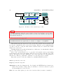
This is the user’s manual for Jane, RWTH’s statistical machine translation toolkit
[Vilar & Stein+ 10, Stein & Vilar+ 11, Vilar & Stein+ 12]. Jane supports state-of-theart techniques for phrase-based and hierarchical phrase-based machine translation. Many
advanced features are implemented in the toolkit, as for instance forced alignment phrase
training for the phrase-based model and several syntactic extensions for the hierarchical
model.
RWTH has been developing Jane during the past years and it was used successfully in
numerous machine translation evaluations. It is developed in C++ with special attention
to clean code, extensibility and efficiency. The toolkit is available under an open source
non-commercial license.
Note that, once compiled, the binaries and scripts intended to be used by the user
are placed in the bin/ directory (the ones in the scripts/ and in the subdirectory
corresponding to your architecture are additional tools that are called automatically).
All programs and scripts have more or less intuitive names, and all of them accept the
--help option. In this way you can find your way around. The main jane and extraction
binary (extractPhrases in the directory corresponding to your architecture) also accept
the option --man for displaying unix-style manual pages.
3
4
CHAPTER 1. INTRODUCTION
Chapter 2
Installation
In this chapter we will guide you through the installation of Jane. Jane has been developed under Linux using gcc and is officially supported for this platform. It may or may
not work on other systems where gcc may be used.
2.1
Software requirements
Jane needs these additional libraries and programs:
SCons Jane uses SCons1 as its build system (minimum required version 1.2). It is
readily available for most Linux distributions. If you do not have permissions
to install SCons system-wide in your computer you may download the scons-local
package from the official SCons page, which you may install locally in any directory
you choose.
SRI LM toolkit Jane uses the language modelling [Stolcke 02] toolkit made available
by the SRI group.2 This toolkit is distributed under another license which you
have to accept before downloading it. Once compiled and installed, you still have
to adapt the headers using the command adaptSriHeaders.sh included in the
jane src/ directory. The include/ directory should be renamed (or linked) as
directory SRI/ in your final installation location.
Jane supports linking with both the standard version and the c space efficient
version of the SRI toolkit (the latter is the default). In order to facilitate having a
SRI installation with both libraries, the object files should be renamed to include
a c suffix.
A typical installation of the SRI toolkit for Jane, including both version of the
libraries, would look like something along these lines
1
2
http://www.scons.org
http://www-speech.sri.com/projects/srilm/
5
6
CHAPTER 2. INSTALLATION
$
$
$
$
$
$
$
$
$
$
$
>
>
$
$
cd ~/src/srilm-1.5.7
export SRILM=‘pwd‘
make World
make World OPTION=_c
export PREFIX=/usr/local/externalTools
mkdir -p $PREFIX/include
mkdir -p $PREFIX/lib
cp -r include $PREFIX/include/SRI
export MT=$SRILM/sbin/machine-type
cp -r lib/$MT/* $PREFIX/lib
for i in lib/${MT}_c/*; do
cp $i $PREFIX/lib/${i/.a/_c.a}
done
cd $PREFIX/include/SRI
~/src/jane/src/adaptSriHeaders.sh
libxml2 This library is readily available and installed in most modern distributions. It
is needed for some legacy code and the dependency will probably be removed in
upcoming releases.
python This programming language is installed by default in virtually every Linux
distribution.
Note
All Jane scripts retrieve the python binary to use by calling env python2. On some
systems, python2 may not point to any python interpreter at all. This problem can
be fixed by adding an appropriate soft link, e.g.:
ln -s /usr/bin/python2.5 /usr/bin/python2
zsh This shell is used in some scripts for distributed operation. It is probably not strictly
necessary, but no guarantees are given. It should be also readily available in most
Linux distribution and trying it out is also a good idea per se.
2.2
Optional dependencies
If they are available, Jane can use following tools and libraries:
Oracle Grid Engine (aka Sun Grid Engine, SGE) Jane may take advantage of the
availability of a grid engine infrastructure3 for distributed operation. More infor3
http://www.oracle.com/technetwork/oem/grid-engine-166852.html
2.2. OPTIONAL DEPENDENCIES
7
mation about configuring Jane for using the grid engine can be found in Section 2.2.1.
Platform LSF Since version 2.1, Jane facilitates the usage of Platform LSF batch
systems4 as an alternative to the Oracle Grid Engine.
Numerical Recipes If the Numerical Recipes [Press & Teukolsky+ 02] library is available, Jane compiles an additional optimization toolkit. This is not needed for
normal operation, but can be used for additional experiments.
cppunit Jane supports unit testing through the cppunit library5 . If you just plan to
use Jane as a translation tool you do not really need this library. It is useful if you
plan to extend Jane, however.
doxygen The code is documented in many parts using the doxygen documentation
system6 . Similar to cppunit, this is only useful if you plan on extending Jane.
OpenFst There is some experimental functionality for word graphs, which makes use
of the OpenFst library7 .
2.2.1
Configuring the grid engine operation
Internally at RWTH we use a wrapper script around the qsub command of the oracle
grid engine. The scripts that interact with the queue make use of this wrapper, called
qsubmit. It is included in the Jane package, in src/Tools/qsubmit. Please have a look
at the script and adapt the first lines according to your queue settings (using the correct
parameter for time and memory specification). Feel free to use this script for you every
day queue usage. If qsubmit is found in your PATH, Jane will use it instead of its local
version.
If you have to include some additional shell scripts in order to be able to interact with
the queue, or if your queue does not accept the qstat and qdel commands, you will have
to adapt the files src/Core/queueSettings.bash and src/Core/queueSettings.zsh.
The if block in this file is there for usage in the different queues available at RWTH. It
may be removed without danger or substituted if needed.
If you want to work on a Platform LSF batch system, you need to use the src/Tools/
bsubmit wrapper script instead of qsubmit. In order to make Jane invoke bsubmit
instead of qsubmit internally, you need to configure the environment accordingly in
src/Core/queueSettings.bash and src/Core/queueSettings.zsh:
export QUEUETYPE=lsf
export QSUBMIT=<path-to-bsubmit>
4
http://www.platform.com/Products/platform-lsf
http://sourceforge.net/apps/mediawiki/cppunit/
6
http://www.doxygen.org
7
http://www.openfst.org
5
8
CHAPTER 2. INSTALLATION
2.3
Compiling
Compiling Jane in most cases just involves calling scons on the main Jane directory.
However you may have to adjust your CPPFLAGS and LDFLAGS environment variables,
so that Jane may find the needed or optional libraries. Standard scons options are
supported, including parallel compilation threads through the -j flag.
Jane uses the standard scons mechanism to find an appropriate compiler (only g++ is
officially supported, though), but you can use the CXX variable to overwrite the default.
Concerning code optimization, Jane is compiled with the -march=native option, which
is only supported starting with g++ version 4.2. For older versions you can specify the
target architecture via the MARCH variable. An example call combining all these variables
(using the sri installation example above)
$ CPPFLAGS=-I/usr/local/externalTools/include \
> LDFLAGS=-L/usr/local/externalTools/lib \
> CXX=g++-4.1 MARCH=opteron scons -j3
2.3.1
Compilation options
Jane accepts different compilation options in the form of VAR=value options. Currently
these options are supported:
SRILIBV Which version of the SRI toolkit library to use, the standard one or the space
optimized one (suffix c). This last one is the default. As discussed in Section 2.1,
the object files of the SRI toolkit must have a c suffix. Use SRILIBV=standard
for using the standard one.
COMPILE You can choose to compile Jane in standard mode (default), in debug or
in profile mode by setting the COMPILE variable in the command line.
VERBOSE With this option you can control the verbosity of the compilation process.
The default is to just show a rotating spinner. If you set the VERBOSE variable to
normal, scons will display messages about its current operation. With the value
full the whole compiler commands will be displayed.
An example compilation command line could be (compilation in debug mode, using
the standard SRI toolkit library, displaying the full compiler command lines and using
three parallel threads).
$ scons -j3 SRILIBV=standard COMPILE=debug VERBOSE=full
scons: Reading SConscript files ...
Checking for C++ library oolm... yes
Checking for C++ library NumericalRecipes... no
Checking for C++ library cppunit... yes
...
2.3. COMPILING
2.3.2
9
Compilation output
The compiled programs reside in the bin/ directory. This directory is self-contained,
you can copy it around as a whole and the programs and scripts contained will use the
appropriate tools. This is useful if you want to pinpoint the exact version you used for
some experiments. Just copy the bin/ directory to your experiments directory and you
are able to reproduce the experiments at any time.
The compilation process also creates a build/ directory where all the object files and
libraries are compiled into. This directory may be safely removed when the compilation
is finished.
10
CHAPTER 2. INSTALLATION
Chapter 3
Short walkthrough
In this chapter we will go through an example use case of the Jane toolkit, starting with
the phrase extraction, following with minimum error rate training on a development
corpus and finally producing a final translation on a test corpus.
This chapter is divided into two sections. In the first section we will run all the
processes locally on one machine. In the second section we will make use of a computer cluster equipped with the Sun Grid Engine for parallel operation. This is the
recommended way of using Jane, especially for large corpora. You can skip one of these
sections if you do not intend to operate Jane in one of these modes. Both sections are
self-contained.
Since Jane supports both—hierarchical and phrase-based translation modes—each
section contains examples for both cases. Make sure that you do not mix configuration
steps from these modes since they will most likely not be compatible.
Note
All examples shown in this chapter are distributed along with Jane.
• Configuration for setting up a hierarchical system running on one machine
examples/local/hierarchical
• Configuration for setting up a phrase-based system running on a local machine
examples/local/phrase-based
• Configuration for setting up a hierarchical system running in a cluster
examples/queue/hierarchical
• Configuration for setting up a phrase-based system running in a cluster
examples/queue/phrase-based
For each of these examples, the data we will use consists of a subset of the data used
in the WMT evaluation campaigns. We will use parts of the 2008 training data, a subset
of the 2006 evaluation data as development corpus and a subset of the 2008 evaluation
data as “test” corpus. Note that the focus of this chapter is to provide you with a basic
11
12
CHAPTER 3. SHORT WALKTHROUGH
feeling of how to use Jane. We use only a limited amount of data in order to speed up
the operation. The optimized parameters found with this data are in no way to be taken
as the best performing ones for the WMT task.
Note
Standard practice is to copy the bin/ directory of the Jane source tree to the directory
containing the data for the experiments. Because the directory is self-contained, this
assures that the results are reproducible in a later point in time. We will assume this
has been done in the example we present below.
Although Jane also supports the moses format for alignments, we usually represent
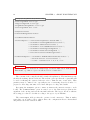
the alignments in the so called in-house “Aachen format”. It looks like this
SENT: 0
S 0 0
S 1 2
S 2 3
SENT: 1
S 0 0
S 1 1
S 2 3
S 3 10
S 4 11
S 6 30
...
The alignments for a sentence pair begin with the SENT: identifier. Then the alignment points follow, one per line. The S in the beginning is for a “Sure” alignment
point. “Possible” alignment points, which may appear in human produced alignments,
are marked with a P. Jane, however, does not distinguish between the two kinds. The
two indices in each line correspond to the words in the source and target sentences,
respectively.
3.1
Running Jane locally
In this section we will go through a typical training-optimization-translation cycle of
Jane running locally on a single computer. We selected only a very small part of the
WMT data (10 000 training sentence pairs, dev and test 100 sentences each) so that
you can go through all the steps in just one session. In this way you can get a feeling
of how to use Jane, but the results obtained here are by no way representative for the
performance of Jane.
3.1. RUNNING JANE LOCALLY
3.1.1
13
Preparing the data
Note
The configuration files for the examples shown in this chapter are located in
examples/local. The data files needed for these examples can be downloaded at:
http://www.hltpr.rwth-aachen.de/jane/files/exampleRun_local.tgz.
The
configuration files expect those files to reside in the same directory as the configuration files themselves.
In our case we concatenate the development and test corpora into one big filter
corpus. This allows us to use the same rule table for optimization and for the final
translation. To be able to use the provided configuration files, you should do the same
by running the following command:
cat german.dev.100 german.test.100 > german.dev.test
3.1.2
Extracting rules
The main program for phrase extraction is trainHierarchical.sh. With the option -h
it gives a list of all its options. For local usage, however, many of them are not relevant.
The options can be specified in the command line or in a config file. As already stated
above, we will use configuration files.
After copying the configuration files (for either the phrase-based or the hierarchical
system) to the same directory as the data you prepared in Chapter 3.1.1 (or Chapter
3.2.1 if you want to run the larger examples) start the rule extraction by running the
following command
$ bin/trainHierarchical.sh --config extract.config
Note
The command for starting rule extraction is the same for phrase-based and hierarchical phrase extraction.
Note
Since running this command typically takes a couple of minutes, you might just go
on reading while Jane is extracting.
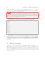
Understanding the general format of the extract.config file
To understand how configuration files work in general, let’s first have a look at the
configuration file for extracting phrase-based rules:
14
CHAPTER 3. SHORT WALKTHROUGH
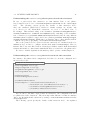
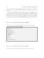
examples/local/phrase-based/extract.config
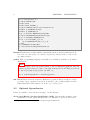
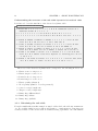
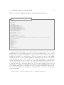
source = german .10000. gz
target = english .10000. gz
alignment = Alignment .10000. gz
filter = german . dev . test
useQueue = false
binarizeM argina ls = false
sortBufferSize =950 M
extractOpts =" - - extractMode = phrase - based - PBT \
-- standard . no nAlign Heuris tic = true \
-- standard . swHeuristic = true \
-- standard . fo rcedSw Heuris tic = true \
-- standard . maxTargetLength =12 \
-- standard . maxSourceLength =6 \
-- f i l t e r I n c o n s i s t e n t C a t e g s = true "
normalizeOpts =" - - standard . IB M1 No rm al iz eP ro bs = false \
-- hierarchical . active = false \
-- count . countVector 1.9 ,2.9 ,3.9"
Important
Since config files are included in a bash script, as such it must follow bash syntax.
This means, e.g., that no spaces are allowed before of after the =.
The contents of the config file should be fairly self-explanatory. The first lines specify
the files the training data is read from. The filter option specifies the corpus that will
be used for filtering the extracted rules in order to limit the size of rule table. This
parameter may be omitted, but—especially in case of extracting hierarchical rules—be
prepared to have huge amounts of free hard disk space for large sized tasks.
By setting the useQueue option to false we instruct the extraction script to work
locally. The sortBufferSize option is carried over to the Unix sort program as the
argument of the -S flag, and sets the internal buffer size. The bigger, the more efficient
the sorting procedure is. Set this according to the specs of your machine.
The extractOpts field specifies the options for rule extraction. Thus it makes
sense that—as we will see later—this is where the configuration files for hierarchical
and phrase-based rule extraction differ.
3.1. RUNNING JANE LOCALLY
15
Understanding the extract.config file for phrase-based rule extraction
In case of phrase-based rule extraction, we first instruct Jane to use phrasebased extraction mode via --extractMode=phrase-based-PBT in the extractOpts
field.
The following options specify the details of this extraction mode.
Since the standard phrase-based extractor’s default settings are mostly only
good choices for the hierarchical extraction, we need to modified some of
its settings: This includes using some heuristics (standard.nonAlignHeuristic,
standard.swHeuristic, standard.forcedSwHeuristic), switching of the normalization of lexical scores (standard.IBM1NormalizeProbs=false) and choosing different
maximum phrase lengths for target and source phrases (standard.maxTargetLength,
standard.maxSourceLength). Furthermore we instruct Jane to filter phrases with inconsistent categories by specifying --filterInconsistentCategs=true.
Since some parts needed for phrase-based rule extraction are calculated in the normalization step, we have to configure another field named normalizeOpts. Here we
instruct Jane to use a modified version of lexical probabilities, switch off the hierarchical
features and include 3 count features with thresholds 1.9, 2.9 and 3.9 to the phrase table.
For a more detailed explanation and further possible options, consult Chapter 4.
Understanding the extract.config file for hierarchical rule extraction
In contrast to the phrase-based configuration, let’s have a look at the configuration for
the hierarchical case:
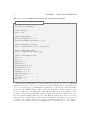
examples/local/hierarchical/extract.config
source = german .10000. gz
target = english .10000. gz
alignment = Alignment .10000. gz
filter = german . dev . test
useQueue = false
binarizeM argina ls = false
sortBufferSize =950 M
extractOpts =" - - extractMode = hierarchical \
-- hierarchical . allowHeuristics = false \
-- standard . no nAlign Heuris tic = true \
-- standard . swHeuristic = true "
As you can see, the first couple of lines are identical to the configuration file used
for phrase-based rule extraction. The most important difference is that we instruct
Jane to use hierarchical rule extraction by setting --extractMode=hierarchical in the
extractOpts field.
The following options specify the details of this extraction mode. As explained
16
CHAPTER 3. SHORT WALKTHROUGH
above, we also need to specify details of the standard features rule. In this case we
stick to the default settings (which are already a good choice for hierarchical extraction), except for setting standard.nonAlignHeuristic=true in order to extract initial
phrases over non-aligned words and for setting standard.swHeuristic=true to ensure
extracting rules for every (single) word seen in the training corpus. For more details on
hierarchical.allowHeuristics have a closer look at Chapter 4.
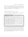
Understanding the general structure of a rule table
After the extraction is finished, you will find (among other files) a file called german.
dev.test.scores.gz. This file holds the extracted rules.
In case of phrase-based extraction, the rule table will look something like this:
examples/somePhrases.phrase-based
1.4013 e -45 0 0 0 0 1 0 0 0 0 0 # X # < unknown - word > # <
unknown - word > # 1 1 1 1 1
0 0 0 0 1 0 0 0 0 0 0 # S # X ~0 # X ~0 # 1 1 1 1 1
0 0 0 0 1 0 0 0 0 0 0 # S # S ~0 X ~1 # S ~0 X ~1 # 1 1 1 1 1
...
2.14007 1.79176 7.75685 6.6614 1 2 1 1 1 1 0 # X # Ich
will # Allow me # 2 2 17 12 2
2.83321 0.693147 11.4204 6.66637 1 4 0.5 2 1 0 0 # X # Ich
will # But I would like # 1 1 17 2 1
3.52636 8.66492 1.13182 5.3448 1 1 2 0.5 1 0 0 # X # Ich
will # I # 0.5 0.5 17 2898 1
2.14007 5.07829 4.88639 5.99186 1 2 1 1 1 1 0 # X # Ich
will # I am # 2 2 17 321 2
2.83321 4.54329 4.90073 6.02781 1 2 1 1 1 0 0 # X # Ich
will # I do # 1 1 17 94 1
...
Each line consists of different fields separated with hashes (“#”). The first field corresponds to the different costs of the rule. It’s subfields contain negative log-probabilities
for the different models specified in extraction. The second field contains the nonterminal associated with the rule. In the standard model, for all the rules except the
first two, it is the symbol X. The third and fourth fields are the source and target parts
of the rule, respectively. Here the non-terminal symbols are identified with a tilde (~)
symbol, with the following number indicating the correspondences between source and
target non-terminals. The fifth field stores the original counts for the rules. Further
fields may be included for additional models.
3.1. RUNNING JANE LOCALLY
17
Important
The hash and the tilde symbols are reserved, i.e. make sure they do not appear in
your data. If they do,, e.g. in urls, we recommend substituting them in the data with
some special codes (e.g. “<HASH>” and “<TILDE>”) and substitute the symbols
back in postprocessing.
Understanding the structure of the rule table for phrase-based rules
Let’s have a closer look at the phrase-based phrase table from above: The scores contained in the first field correspond to
1. Phrase source-to-target score
2. Phrase target-to-source score
3. Lexical source-to-target score (not normalized to the phrase length)
4. Lexical target-to-source score (not normalized to the phrase length)
5. Phrase penalty (always 1)
6. Word penalty (number words generated)
7. Source-to-target length ratio
8. Target-to-source length ratio
9. Binary flag: Count > 1.9
10. Binary flag: Count > 2.9
11. Binary flag: Count > 3.9
18
CHAPTER 3. SHORT WALKTHROUGH
Understanding the structure of the rule table layout for hierarchical rules
Let’s have a look at the first lines of the hierarchical phrase table.
examples/somePhrases.hierarchical
1.4013 e -45 0 0 0 0 1 0 0 0 0 1 # X # < unknown - word > # <
unknown - word > # 1 1 1 1 1
0 0 0 0 1 0 0 0 0 0 0 # S # X ~0 # X ~0 # 1 1 1 1 1
0 0 0 0 1 0 0 0 0 0 1 # S # S ~0 X ~1 # S ~0 X ~1 # 1 1 1 1 1
...
1.81916 4.58859 4.88639 5.99186 1 2 1 1 1 1 0 # X # Ich
will X ~0 # I am X ~0 # 3 3 18.5 295.067 4
2.07047 2.57769 4.90073 6.02781 1 2 1 1 1 1 0 # X # Ich
will X ~0 # I do X ~0 # 2.33333 4 18.5 52.6666 4
1.76509 2.75207 5.22612 6.1557 1 2 1 1 1 1 0 # X # Ich
will X ~0 # I must X ~0 # 3.16667 3.33333 18.5 52.25 5
2.00148 0 20.9296 7.21078 1 6 0.333333 3 1 1 0 # X # Ich
will X ~0 # I shall restrict myself to raising X ~0 # 2.5
3 18.5 3 3
1.81916 0 16.2028 6.53239 1 5 0.4 2.5 1 1 0 # X # Ich will
X ~0 # I want to make it X ~0 # 3 2.5 18.5 2.5 3
...
The scores of the hierarchical phrase table correspond to the following model scores:
1. Phrase source-to-target score
2. Phrase target-to-source score
3. Lexical source-to-target score
4. Lexical target-to-source score
5. Phrase penalty (always 1)
6. Word penalty (number of words generated)
7. Source-to-target length ratio
8. Target-to-source length ratio
9. Binary flag: isHierarchical
10. Binary flag: isPaste
11. Binary flag: glueRule
3.1.3
Binarizing the rule table
For such a small task as in this example we may load the whole rule table into main memory. For real-life tasks, however, this would require too much memory. Jane supports
a binary format for rule tables with on-demand-loading capabilities. We will binarize
3.1. RUNNING JANE LOCALLY
19
the rule table—regardless of having extracted in phrase-based mode or in hierarchical
mode—with the following command:
$ bin/rules2Binary.x86_64-standard \
> --file german.dev.test.scores.gz \
> --out german.dev.test.scores.bin
This will create a new file named german.dev.test.scores.bin.
3.1.4
Minimum error rate training
In the next step we will perform minimum error rate training on the development set.
For this first we must create a basic configuration file for the decoder, specifying the
options we will use.
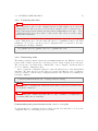
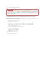
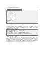
The jane.config configuration file in general
The config file is divided into different sections, each of them labelled with some text
in square brackets ([ ]). All of the names start with a Jane identifier. The reason
for this is because the configuration file may be shared among several programs1 . The
same options can be specified in the command line by specifying the fully qualified
option name, without the Jane identifier. For example, the option fileIn in block
[Jane.singleBest] can be specified in the command line as --singleBest.fileIn. In
this way we can translate another input file without needing to alter the config file.
1
This feature is rarely used any more
20
CHAPTER 3. SHORT WALKTHROUGH
The jane.config configuration file for the phrase-based decoder
In case of a phrase-based system, create a jane.config file with the following contents
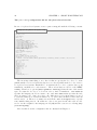
examples/local/phrase-based/jane.config
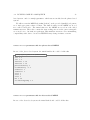
[ Jane ]
decoder = scss
[ Jane . nBest ]
size = 20
[ Jane . SCSS ]
o b s e r v a t i o n H i s t o g r a m S i z e = 100
l e x i c a l H i s t o g r a m S i z e = 16
r e o r d e r i n g H i s t o g r a m S i z e = 32
reorderingConstraintMaximumRuns = 2
reorderingMaximumJumpWidth = 5
f i r s t W o r d L M L o o k A h e a d P r u n i n g = true
p h r a s e O n l y L M L o o k A h e a d P r u n i n g = false
m a x T a r g e t P h r a s e L e n g t h = 11
maxSourcePhraseLength = 6
[ Jane . SCSS . LM ]
file = english . lm .4 gram . gz
order = 4
[ Jane . SCSS . rules ]
file = german . dev . test . scores . bin
whichCosts = 0 ,1 ,2 ,3 ,4 ,5 ,6 ,7 ,8 ,9 ,10
costsNames = s2t , t2s , ibm1s2t , ibm1t2s , phrasePenalty , wordPenalty , s2tRatio , t2sRatio , cnt1 , cnt2 , cnt3
[ Jane . scalingFactors ]
s2t = 0.1
t2s = 0.1
ibm1s2t = 0.05
ibm1t2s = 0.05
phrasePenalty = 0
wordPenalty = -0.1
s2tRatio = 0
t2sRatio = 0
cnt1 = 0
cnt2 = 0
cnt3 = 0
LM = 0.25
reorderingJump = 0.1
The most important thing to note here is that we specify the decoder to be scss
(which stands for Source Cardinality Synchronous Search) which is the decoder of choice
for a phrase-based system. Furthermore, we instruct the decoder to generate the top 20
translation candidates for each sentence. These nbest lists are used for the MERT
training. Then lots of options (*HistogramSize, *Pruning) define the size of the search
space we want the decoder to look at in order to find a translation. Jane.SCSS.LM
specifies the language model we want to use, and Jane.SCSS.rules specifies the rule
table we want to use. Since we refer to the different scores by their names, we need
to tell Jane which score resides in which row, e.g. s2t resides in field 0, t2s resides in
field 1, and so on. These score names are used in the Jane.scalingFactors to specify
some initial scaling factors. In addition to the scores given in the rule table we also
need to set the weights for the language model (LM) and the costs for a reordering jump
(reorderingJump).
More details about the configuration file are discussed in Chapter 5.
3.1. RUNNING JANE LOCALLY
21
The jane.config configuration file for the hierarchical decoder
In case of the hierarchical system, create a jane.config file with the following contents
examples/local/hierarchical/jane.config
[ Jane ]
decoder = cubeGrow
[ Jane . nBest ]
size = 20
[ Jane . CubeGrow ]
lmNbestHeuristic = 50
maxCGBufferSize = 200
[ Jane . CubeGrow . LM ]
file = english . lm .4 gram . gz
[ Jane . CubeGrow . rules ]
file = german . dev . test . scores . bin
[ Jane . scalingFactors ]
s2t = 0.1
t2s = 0.1
ibm1s2t = 0.1
ibm1t2s = 0.1
phrasePenalty = 0.1
wordPenalty = -0.1
s2tRatio = 0.1
t2sRatio = 0.1
isHierarchical = 0.1
isPaste = 0.1
glueRule = 0.1
LM = 0.2
The most important thing to note here is that we specify the decoder to be cubeGrow
which is the decoder of choice for a hierarchical system. Furthermore, we instruct the
decoder to generate the top 20 translation candidates for each sentence. These nbest lists
are used for the MERT training. Then options specifying more details of the decoding
process are listed in Jane.CubeGrow. Jane.CubeGrow.LM specifies the language model
we want to use, and Jane.CubeGrow.rules specifies the rule table we want to use. The
last section shows initial scaling factors for the different models used. Since hierarchical
extraction is the default setup of Jane, Jane automatically knows which rows correspond
to what scores—and we just need to specify the initial scaling factors. Note that we
22
CHAPTER 3. SHORT WALKTHROUGH
here have some different additional weighting factors: LM—like in case of the phrasebased system—and for example glueRule—which was not included in the phrase-based
system.
We will now run the MERT algorithm [Och 03] on the provided (small) development
set to find appropriate values for them. The lambda values for the MERT are stored
in so-called lambda files. The initial values for the MERT are stored in a file called
lambda.initial. These files contain the same scaling factors as the jane.config file
we created before, but without equal signs. This small inconvenience is for maintaining
compatibility with other tools used at RWTH. It may change in future versions.
lambda.initial parameters file for phrase-based MERT
In case of the phrase-based system, the initial lambda file could look like this
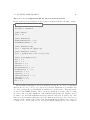
examples/local/phrase-based/lambda.initial
s2t 0.1
t2s 0.1
ibm1s2t 0.05
ibm1t2s 0.05
phrasePenalty 0
wordPenalty -0.1
s2tRatio 0
t2sRatio 0
cnt1 0
cnt2 0
cnt3 0
LM 0.25
reorderingJump 0.1
lambda.initial parameters file for hierarchical MERT
In case of the hierarchical system, the initial lambda file could look like this
3.1. RUNNING JANE LOCALLY
23
examples/local/hierarchical/lambda.initial
s2t 0.1
t2s 0.1
ibm1s2t 0.1
ibm1t2s 0.1
phrasePenalty 0.1
wordPenalty -0.1
s2tRatio 0.1
t2sRatio 0.1
isHierarchical 0.1
isPaste 0.1
glueRule 0.1
LM 0.2
Running MERT
We will now optimize using the german.dev.100 file as the development set. The reference translation can be found in english.dev.100. The command for performing
minimum error rate training is
$
>
>
>
bin/localOptimization.sh --method mert \
--janeConfig jane.config \
--dev german.dev.100 --reference english.dev.100 \
--init lambda.initial --optDir opt --randomRestarts 10
You will see some logging messages about the translation process. This whole process
will take some time to finish.
You can observe that a directory opt/ has been created which holds the n-best
lists that Jane generates together with some auxiliary files for the translation process.
Specifically, by examining the nBestOptimize.*.log files you can see the evolution of
the optimization process. Currently only optimizing for the BLEU score is supported,
but different extern error scorer can be included as an extern error scorer, too.
24
CHAPTER 3. SHORT WALKTHROUGH
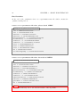
Final Lambdas
At the end of the optimization there is a opt/lambda.final file which contains the
optimized scaling factors.
lambda.finial parameters file after phrase-based MERT
examples/local/phrase-based/lambda.final
s2t 0. 06 45 03 11 157 38 30 5
t2s 0. 02 23 32 87 814 10 19 5
ibm1s2t 0. 115763 502220 802
ibm1t2s -0.0926093658987379
phrasePenalty -0.0906163708734068
wordPenalty -0.112589503827774
s2tRatio -0.0175426263656464
t2sRatio -0.00742491151019232
cnt1 0.1 234259 965861 34
cnt2 0.1 298500 439062 02
cnt3 0 .0 60 79 85 51 55 73 98 2
LM 0.1 41997 281727 464
reorderingJump 0.0 20 54 58 55 81 13 92 8
lambda.finial parameters file after hierarchical MERT
examples/local/hierarchical/lambda.final
s2t 0 .15640 374892 2424
t2s 0. 01 03 27 57 790 72 47 8
ibm1s2t 0. 025 88 05 08 07 62 00 6
ibm1t2s 0. 023 07 66 26 88 86 11 7
phrasePenalty -0.0358096401282086
wordPenalty -0.0988531371883096
s2tRatio 0.14 597281 489425 2
t2sRatio -0.221343456126843
isHierarchical 0.0 99 13 46 05 51 79 33 4
isPaste 0. 014 62 80 18 66 54 63 4
glueRule 0 . 0 08 0 8 23 7 6 32 60 28 7 3
LM 0.1 60487 489358 477
Note
Your results will vary, due to the random restarts of the algorithm.
3.1. RUNNING JANE LOCALLY
3.1.5
25
Translating the test data
We must now take the optimized scaling factors we found in last section and update
them in the jane.config file.
Note
Do not forget to add the equal sign if you copy & paste the contents of the lambda.
final file.
We will also specify the test corpus we want to translate.
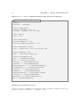
Final jane.opt.config configuration file for the phrase-based decoder
examples/local/phrase-based/jane.opt.config
[ Jane ]
decoder = scss
[ Jane . singleBest ]
fileIn = german . test .100
fileOut = german . test .100. hyp
[ Jane . nBest ]
size = 100
[ Jane . SCSS ]
o b s e r v a t i o n H i s t o g r a m S i z e = 100
l e x i c a l H i s t o g r a m S i z e = 16
r e o r d e r i n g H i s t o g r a m S i z e = 32
reorderingConstraintMaximumRuns = 2
reorderingMaximumJumpWidth = 5
f i r s t W o r d L M L o o k A h e a d P r u n i n g = true
p h r a s e O n l y L M L o o k A h e a d P r u n i n g = false
m a x T a r g e t P h r a s e L e n g t h = 11
maxSourcePhraseLength = 6
[ Jane . SCSS . LM ]
file = english . lm .4 gram . gz
order = 4
[ Jane . SCSS . rules ]
file = german . dev . test . scores . bin
whichCosts = 0 ,1 ,2 ,3 ,4 ,5 ,6 ,7 ,8 ,9 ,10
costsNames = s2t , t2s , ibm1s2t , ibm1t2s , phrasePenalty , wordPenalty , s2tRatio , t2sRatio , cnt1 , cnt2 , cnt3
[ Jane . scalingFactors ]
s2t = 0. 0 64 5 03 11 1 57 3 83 05
t2s = 0. 0 22 3 32 87 8 14 1 01 95
ibm1s2t = 0. 115 763 502 2208 02
ibm1t2s = -0.0926093658987379
phrasePenalty = -0.0906163708734068
wordPenalty = -0.112589503827774
s2tRatio = -0.0175426263656464
t2sRatio = -0.00742491151019232
cnt1 = 0.12 342 599 658 6134
cnt2 = 0.12 985 004 390 6202
cnt3 = 0. 0 60 7 98 55 1 55 7 39 82
LM = 0. 141 997 281 7274 64
reorderingJump = 0. 0 20 54 5 85 5 81 13 9 28
26
CHAPTER 3. SHORT WALKTHROUGH
Final jane.opt.config configuration file for the hierarchical decoder
examples/local/hierarchical/jane.opt.config
[ Jane ]
decoder = cubePrune
[ Jane . singleBest ]
fileIn = german . test .100
fileOut = german . test .100. hyp
[ Jane . nBest ]
size = 100
[ Jane . CubePrune ]
generationNbest = 100
o b se r v a t i o n H i s t o g r a m S i z e = 50
[ Jane . CubePrune . rules ]
file = german . dev . test .100. scores . bin
[ Jane . CubePrune . LM ]
file = english . lm .4 gram . gz
[ Jane . scalingFactors ]
s2t = 0 .15640 374892 2424
t2s = 0. 01 03 27 57 790 72 47 8
ibm1s2t = 0. 025 88 05 08 0762 00 6
ibm1t2s = 0. 023 07 66 26 8886 11 7
phrasePenalty = -0.0358096401282086
wordPenalty = -0.0988531371883096
s2tRatio = 0.14 597281 489425 2
t2sRatio = -0.221343456126843
isHierarchical = 0.0 99 13 46 05 51 79 33 4
isPaste = 0. 014 62 80 18 6654 63 4
glueRule = 0 . 0 08 0 8 23 7 6 32 6 0 28 7 3
LM = 0.1 60487 489358 477
Starting the translation process
We are now ready to translate the test data. For this—regardless of using a phrase-based
system or a hierarchical system—we just have to type
3.2. RUNNING JANE IN A SGE QUEUE
27
$ bin/jane.x86_64-standard --config jane.opt.config
The results are then located in german.test.100.hyp.
3.2
Running Jane in a SGE queue
In this section we will go through the whole process of setting up a Jane system in an
environment equipped with the SGE grid engine. We will assume that Jane has been
properly configure for queue usage (see Section 2.2.1). The examples will make use of
the qsubmit wrapper script provided with Jane. If you do not wish to use the tool, you
may easily adapt the commands accordingly.
3.2.1
Preparing the data
Note
The configuration files for the examples shown in this chapter are located in
examples/queue. The data files needed for these examples can be downloaded at:
http://www.hltpr.rwth-aachen.de/jane/files/exampleRun_queue.tgz.
The
configuration files expect those files to reside in the same directory as the configuration files themselves.
We selected only a small part of the WMT data (100 000 training sentence pairs, dev
and test 100 sentences each) so that you can go through all the steps in just one session.
In this way you can get a feeling of how to use Jane, but the results obtained here are
by no way representative for the performance of Jane.
In our case we concatenate the development and test corpora into one big filter
corpus. This allows us to use the same rule table for optimization and for the final
translation. To be able to use the provided configuration files, you should do the same
by running the following command:
cat german.dev.100 german.test.100 > german.dev.test
3.2.2
Extracting rules
The main program for phrase extraction is trainHierarchical.sh. With the option -h
it gives a list of all its options. For local usage, however, many of them are not relevant.
The options can be specified in the command line or in a config file. As already stated
above, we will use configuration files.
After copying the configuration files (for either the phrase-based or the hierarchical
system) to the same directory as the data you prepared in Chapter 3.1.1 (or Chapter
3.2.1 if you want to run the larger examples) start the rule extraction by running the
following command
28
CHAPTER 3. SHORT WALKTHROUGH
$ bin/trainHierarchical.sh --config extract.config
Note
The command for starting rule extraction is the same for phrase-based and hierarchical phrase extraction.
Note
Since running this command typically takes a couple of minutes, you might just go
on reading while Jane is extracting.
Understanding the general format of the extract.config file
To understand how configuration files work in general, let’s first have a look at the
configuration file for extracting phrase-based rules.
The contents of the config file should be fairly self-explanatory. The first lines specify
the file the training data is read from. The filter option specifies the corpus which will
be used for filtering the extracted rules in order to limit the size of the rule table. This
parameter may be omitted, but—especially in case of extracting hierarchical rules—be
prepared to have huge amounts of free hard disk space for large sized tasks.
Important
Since config files are included in a bash script, as such it must follow bash syntax.
This means, e.g., that no spaces are allowed before of after the =.
Setting the useQueue option to true we instruct the extraction script to use the SGE
queue. The sortBufferSize option is carried over to sort program as the argument of
the -S flag, and sets the internal buffer size, The bigger, the more efficient the sorting
procedure is. Set this according to the specs of your machines.
Most of the options of the config file then refer to setting memory and time specifications for the jobs that will be started. You can see that we included comments with
rough guidelines of how much time and memory each step takes. The file was generated
with the command
$ bin/trainHierarchical.sh --exampleConfig > extract.config
and then adapting it accordingly.
The extractOpts field specifies the options for phrase extraction. Thus it makes
sense that—as we will see later—this is where the configuration files for hierarchical and
phrase-based rule extraction differ.
3.2. RUNNING JANE IN A SGE QUEUE
examples/queue/phrase-based/extract.config
source = german .100000. gz
target = english .100000. gz
alignment = Alignment .100000. gz
filter = german . dev . test
useQueue = true
jobName = janeDemo
addition alModels =""
# All sort operations use this buffer size
sortBufferSize =950 M
# Extraction options , look into the help of extractPhrases for a complete list of options
extractOpts =" - - extractMode = phrase - based - PBT \
-- standard . non Ali gnHe uri sti c = true \
-- standard . swHeuristic = true \
-- standard . for ced SwHe uri sti c = true \
-- standard . maxTargetLength =12 \
-- standard . maxSourceLength =6 \
-- f i l t e r I n c o n s i s t e n t C a t e g s = true "
# Time and memory greatly depend on the corpus ( and the alignments ) . No good
# default estimate can be given here
extractMem =1
extractTime =0:30:00
# The second run will need more memory than the first one .
# Time should be similar , though
extractMem2ndRun =1
ex tra ctT ime2 ndR un =0:30:00
# The higher this number , the lower the number of jobs but with higher requirements
extractSplitStep =5000
# Count threshold for hierarchical phrases
# You should specify ALL THREE thresholds , one alone will not work
s o u r c e C o u n t T h r e s h o l d =0
t a r g e t C o u n t T h r e s h o l d =0
r ea lC o un t Th re s ho l d =2
# The lower this number , the higher the number of normalization jobs
splitCou ntsStep =500000
# If using useQueue , adjust the memory requirements and the buffer size for sorting appropriately
sortCountsMem =1
sortCountsTime =0:30:00
# Joining the counts
# Memory efficient , time probably not so much
joinCountsMem =1
joinCountsTime =0:30:00
bi nar ize Marg ina ls = false
# Sorting the source marginals
# These are relatively small , so probably not much resources are needed
s o r t S o u r c e M a r g i n a l s M e m =1
s o r t S o u r c e M a r g i n a l s T i m e =0:30:00
# Resources for binarization of source counts should be fairly reasonable for standard dev / test corpora
# Warning , this also includes joining
b i n a r i z e S o u r c e M a r g i n a l s W r i t e D e p t h =0
b i n a r i z e S o u r c e M a r g i n a l s M e m =1
b i n a r i z e S o u r c e M a r g i n a l s T i m e =0:30:00
# Resources for filtering source marginals
f i l t e r S o u r c e M a r g i n a l s M e m =1
f i l t e r S o u r c e M a r g i n a l s T i m e =4:00:00
# Sorting the target marginals
# The target marginals files are much bigger than the source marginals , more time is needed
s o r t T a r g e t M a r g i n a l s M e m =1
s o r t T a r g e t M a r g i n a l s T i m e =0:30:00
# All target marginals must be extracted . This operation is therefore more resource
# intensive than the source marginals . Memory requirements can however be controlled
# by the writeDepth parameter
b i n a r i z e T a r g e t M a r g i n a l s W r i t e D e p t h =0
b i n a r i z e T a r g e t M a r g i n a l s M e m =1
b i n a r i z e T a r g e t M a r g i n a l s T i m e =0:30:00
# Resources for filtering target marginals
f i l t e r T a r g e t M a r g i n a l s M e m =1
f i l t e r T a r g e t M a r g i n a l s T i m e =4:00:00
# Normalization is more or less time and memory efficient
normalizeOpts =" - - standard . IB M1 N or m al iz e Pr o bs = false \
-- hierarchical . active = false \
-- count . countVector 1.9 ,2.9 ,3.9"
n or m al iz e Co un t sM e m =1
n o r m al i z e C o u n t sT i m e =0:30:00
# This is basically a ( z ) cat , so no big deal here either
joinScoresMem =1
joinScoresTime =0:30:00
29
30
CHAPTER 3. SHORT WALKTHROUGH
Understanding the extract.config file for phrase-based rule extraction
In case of phrase-based rule extraction, we first instruct Jane to use phrasebased extraction mode via --extractMode=phrase-based-PBT in the extractOpts
field.
The following options specify the details of this extraction mode.
Since the standard phrase-based extractor’s default settings are mostly only
good choices for the hierarchical extraction, we need to modified some of
its settings: This includes using some heuristics (standard.nonAlignHeuristic,
standard.swHeuristic, standard.forcedSwHeuristic), switching of the normalization of lexical scores (standard.IBM1NormalizeProbs=false) and choosing different
maximum phrase lengths for target and source phrases (standard.maxTargetLength,
standard.maxSourceLength). Furthermore we instruct Jane to filter phrases with inconsistent categories by specifying --filterInconsistentCategs=true.
Since some parts needed for phrase-based rule extraction are calculated in the normalization step, we have to configure another field named normalizeOpts. Here we
instruct Jane to use a modified version of lexical probabilities, switch off the hierarchical
features and include 3 count features with thresholds 1.9, 2.9 and 3.9 to the phrase table.
For a more detailed explanation and further possible options, consult Chapter 4.
Understanding the extract.config file for hierarchical rule extraction
In contrast to the phrase-based configuration, let’s have a look at the configuration for
the hierarchical rule extraction:
As you can see, the first couple of lines are identical to the configuration file used
for phrase-based rule extraction. The most important difference is that we instruct
Jane to use hierarchical rule extraction by setting --extractMode=hierarchical in the
extractOpts field.
The following options specify the details of this extraction mode. As explained
above, we also need to specify details of the standard features rule. In this case we
stick to the default settings (which are already a good choice for hierarchical extraction), except for setting standard.nonAlignHeuristic=true in order to extract initial
phrases over non-aligned words and for setting standard.swHeuristic=true to ensure
extracting rules for every (single) word seen in the training corpus. For more details on
hierarchical.allowHeuristics have a closer look at Chapter 4.
3.2. RUNNING JANE IN A SGE QUEUE
examples/queue/hierarchical/extract.config
source = german .100000. gz
target = english .100000. gz
alignment = Alignment .100000. gz
filter = german . dev . test
useQueue = true
jobName = janeDemo
addition alModels =""
# All sort operations use this buffer size
sortBufferSize =950 M
# Extraction options , look into the help of extractPhrases for a complete list of options
extractOpts =" - - extractMode = hierarchical \
-- hierarchical . allowHeuristics = false \
-- standard . non Ali gnHe uri sti c = true \
-- standard . swHeuristic = true "
# Time and memory greatly depend on the corpus ( and the alignments ) . No good
# default estimate can be given here
extractMem =1
extractTime =0:30:00
# The second run will need more memory than the first one .
# Time should be similar , though
extractMem2ndRun =1
ex tra ctT ime2 ndR un =0:30:00
# The higher this number , the lower the number of jobs but with higher requirements
extractSplitStep =5000
# Count threshold for hierarchical phrases
# You should specify ALL THREE thresholds , one alone will not work
s o u r c e C o u n t T h r e s h o l d =0
t a r g e t C o u n t T h r e s h o l d =0
r ea lC o un t Th re s ho l d =2
# The lower this number , the higher the number of normalization jobs
splitCou ntsStep =500000
# If using useQueue , adjust the memory requirements and the buffer size for sorting appropriately
sortCountsMem =1
sortCountsTime =0:30:00
# Joining the counts
# Memory efficient , time probably not so much
joinCountsMem =1
joinCountsTime =0:30:00
bi nar ize Marg ina ls = false
# Sorting the source marginals
# These are relatively small , so probably not much resources are needed
s o r t S o u r c e M a r g i n a l s M e m =1
s o r t S o u r c e M a r g i n a l s T i m e =0:30:00
# Resources for binarization of source counts should be fairly reasonable for standard dev / test corpora
# Warning , this also includes joining
b i n a r i z e S o u r c e M a r g i n a l s W r i t e D e p t h =0
b i n a r i z e S o u r c e M a r g i n a l s M e m =1
b i n a r i z e S o u r c e M a r g i n a l s T i m e =0:30:00
# Resources for filtering source marginals
f i l t e r S o u r c e M a r g i n a l s M e m =1
f i l t e r S o u r c e M a r g i n a l s T i m e =4:00:00
# Sorting the target marginals
# The target marginals files are much bigger than the source marginals , more time is needed
s o r t T a r g e t M a r g i n a l s M e m =1
s o r t T a r g e t M a r g i n a l s T i m e =0:30:00
# All target marginals must be extracted . This operation is therefore more resource
# intensive than the source marginals . Memory requirements can however be controlled
# by the writeDepth parameter
b i n a r i z e T a r g e t M a r g i n a l s W r i t e D e p t h =0
b i n a r i z e T a r g e t M a r g i n a l s M e m =1
b i n a r i z e T a r g e t M a r g i n a l s T i m e =0:30:00
# Resources for filtering target marginals
f i l t e r T a r g e t M a r g i n a l s M e m =1
f i l t e r T a r g e t M a r g i n a l s T i m e =4:00:00
# Normalization is more or less time and memory efficient
normalizeOpts =""
n or m al iz e Co un t sM e m =1
n o r m al i z e C o u n t sT i m e =0:30:00
# This is basically a ( z ) cat , so no big deal here either
joinScoresMem =1
joinScoresTime =0:30:00
31
32
CHAPTER 3. SHORT WALKTHROUGH
Understanding the general structure of a rule table
After the extraction is finished, you will find (among other files) a file called german.
dev.test.scores.gz. This file holds the extracted rules.
In case of phrase-based extraction, the rule table will look something like this:
examples/somePhrases.phrase-based
1.4013 e -45 0 0 0 0 1 0 0 0 0 0 # X # < unknown - word > # <
unknown - word > # 1 1 1 1 1
0 0 0 0 1 0 0 0 0 0 0 # S # X ~0 # X ~0 # 1 1 1 1 1
0 0 0 0 1 0 0 0 0 0 0 # S # S ~0 X ~1 # S ~0 X ~1 # 1 1 1 1 1
...
2.14007 1.79176 7.75685 6.6614 1 2 1 1 1 1 0 # X # Ich
will # Allow me # 2 2 17 12 2
2.83321 0.693147 11.4204 6.66637 1 4 0.5 2 1 0 0 # X # Ich
will # But I would like # 1 1 17 2 1
3.52636 8.66492 1.13182 5.3448 1 1 2 0.5 1 0 0 # X # Ich
will # I # 0.5 0.5 17 2898 1
2.14007 5.07829 4.88639 5.99186 1 2 1 1 1 1 0 # X # Ich
will # I am # 2 2 17 321 2
2.83321 4.54329 4.90073 6.02781 1 2 1 1 1 0 0 # X # Ich
will # I do # 1 1 17 94 1
...
Each line consists of different fields separated with hashes (“#”). The first field corresponds to the different costs of the rule. It’s subfields contain negative log-probabilities
for the different models specified in extraction. The second field contains the nonterminal associated with the rule. In the standard model, for all the rules except the
first two, it is the symbol X. The third and fourth fields are the source and target parts
of the rule, respectively. Here the non-terminal symbols are identified with a tilde (~)
symbol, with the following number indicating the correspondences between source and
target non-terminals. The fifth field stores the original counts for the rules. Further
fields may be included for additional models.
Important
The hash and the tilde symbols are reserved, i.e. make sure they do not appear in
your data. If they do,, e.g. in urls, we recommend substituting them in the data with
some special codes (e.g. “<HASH>” and “<TILDE>”) and substitute the symbols
back in postprocessing.
Understanding the structure of the rule table for phrase-based rules
Let’s have a closer look at the phrase-based phrase table from above: The scores contained in the first field correspond to
3.2. RUNNING JANE IN A SGE QUEUE
33
1. Phrase source-to-target score
2. Phrase target-to-source score
3. Lexical source-to-target score (not normalized to the phrase length)
4. Lexical target-to-source score (not normalized to the phrase length)
5. Phrase penalty (always 1)
6. Word penalty (number words generated)
7. Source-to-target length ratio
8. Target-to-source length ratio
9. Binary flag: Count > 1.9
10. Binary flag: Count > 2.9
11. Binary flag: Count > 3.9
Understanding the structure of the rule table layout for hierarchical rules
Let’s have a look at the first lines of the hierarchical phrase table.
examples/somePhrases.hierarchical
1.4013 e -45 0 0 0 0 1 0 0 0 0 1 # X # < unknown - word > # <
unknown - word > # 1 1 1 1 1
0 0 0 0 1 0 0 0 0 0 0 # S # X ~0 # X ~0 # 1 1 1 1 1
0 0 0 0 1 0 0 0 0 0 1 # S # S ~0 X ~1 # S ~0 X ~1 # 1 1 1 1 1
...
1.81916 4.58859 4.88639 5.99186 1 2 1 1 1 1 0 # X # Ich
will X ~0 # I am X ~0 # 3 3 18.5 295.067 4
2.07047 2.57769 4.90073 6.02781 1 2 1 1 1 1 0 # X # Ich
will X ~0 # I do X ~0 # 2.33333 4 18.5 52.6666 4
1.76509 2.75207 5.22612 6.1557 1 2 1 1 1 1 0 # X # Ich
will X ~0 # I must X ~0 # 3.16667 3.33333 18.5 52.25 5
2.00148 0 20.9296 7.21078 1 6 0.333333 3 1 1 0 # X # Ich
will X ~0 # I shall restrict myself to raising X ~0 # 2.5
3 18.5 3 3
1.81916 0 16.2028 6.53239 1 5 0.4 2.5 1 1 0 # X # Ich will
X ~0 # I want to make it X ~0 # 3 2.5 18.5 2.5 3
...
The scores of the hierarchical phrase table correspond to the following model scores:
1. Phrase source-to-target score
2. Phrase target-to-source score
3. Lexical source-to-target score
34
CHAPTER 3. SHORT WALKTHROUGH
4. Lexical target-to-source score
5. Phrase penalty (always 1)
6. Word penalty (number of words generated)
7. Source-to-target length ratio
8. Target-to-source length ratio
9. Binary flag: isHierarchical
10. Binary flag: isPaste
11. Binary flag: glueRule
3.2.3
Binarizing the rule table
For such a small task as in this example we may load the whole rule table into main memory. For real-life tasks, however, this would require too much memory. Jane supports
a binary format for rule tables with on-demand-loading capabilities. We will binarize
the rule table—regardless of having extracted in phrase-based mode or in hierarchical
mode—with the following command:
$ bin/rules2Binary.x86_64-standard \
> --file german.dev.test.scores.gz \
> --out german.dev.test.scores.bin
3.2.4
Minimum error rate training
In the next step we will perform minimum error rate training on the development set.
For this first we must create a basic configuration file for the decoder, specifying the
options we will use.
The jane.config configuration file in general
The config file is divided into different sections, each of them labelled with some text
in square brackets ([ ]). All of the names start with a Jane identifier. The reason
for this is because the configuration file may be shared among several programs2 . The
same options can be specified in the command line by specifying the fully qualified
option name, without the Jane identifier. For example, the option fileIn in block
[Jane.singleBest] can be specified in the command line as --singleBest.fileIn. In
this way we can translate another input file without needing to alter the config file.
2
This feature is rarely used any more
3.2. RUNNING JANE IN A SGE QUEUE
35
The jane.config configuration file for the phrase-based decoder
examples/queue/phrase-based/jane.config
[ Jane ]
decoder = scss
[ Jane . nBest ]
size = 20
[ Jane . SCSS ]
o b s e r v a t i o n H i s t o g r a m S i z e = 100
l e x i c a l H i s t o g r a m S i z e = 16
r e o r d e r i n g H i s t o g r a m S i z e = 32
reorderingConstraintMaximumRuns = 2
reorderingMaximumJumpWidth = 5
f i r s t W o r d L M L o o k A h e a d P r u n i n g = true
p h r a s e O n l y L M L o o k A h e a d P r u n i n g = false
m a x T a r g e t P h r a s e L e n g t h = 11
maxSourcePhraseLength = 6
[ Jane . SCSS . LM ]
file = english . lm .4 gram . gz
order = 4
[ Jane . SCSS . rules ]
file = german . dev . test . scores . bin
whichCosts = 0 ,1 ,2 ,3 ,4 ,5 ,6 ,7 ,8 ,9 ,10
costsNames = s2t , t2s , ibm1s2t , ibm1t2s , phrasePenalty , wordPenalty , s2tRatio , t2sRatio , cnt1 , cnt2 , cnt3
[ Jane . scalingFactors ]
s2t = 0.1
t2s = 0.1
ibm1s2t = 0.05
ibm1t2s = 0.05
phrasePenalty = 0
wordPenalty = -0.1
s2tRatio = 0
t2sRatio = 0
cnt1 = 0
cnt2 = 0
cnt3 = 0
LM = 0.25
reorderingJump = 0.1
The most important thing to note here is that we specify the decoder to be scss
(which stands for Source Cardinality Synchronous Search) which is the decoder of choice
for a phrase-based system. Furthermore, we instruct the decoder to generate the top 20
translation candidates for each sentence. These nbest lists are used for the MERT
training. Then lots of options (*HistogramSize, *Pruning) define the size of the search
space we want the decoder to look at in order to find a translation. Jane.SCSS.LM
specifies the language model we want to use, and Jane.SCSS.rules specifies the rule
table we want to use. Since we refer to the different scores by their names, we need
to tell Jane which score resides in which row, e.g. s2t resides in field 0, t2s resides in
field 1, and so on. These score names are used in the Jane.scalingFactors to specify
some initial scaling factors. In addition to the scores given in the rule table we also
need to set the weights for the language model (LM) and the costs for a reordering jump
(reorderingJump).
More details about the configuration file are discussed in Chapter 5.
36
CHAPTER 3. SHORT WALKTHROUGH
The jane.config configuration file for the hierarchical decoder
examples/queue/hierarchical/jane.config
[ Jane ]
decoder = cubePrune
[ Jane . nBest ]
size = 50
[ Jane . CubePrune ]
generationNbest = 100
o b se r v a t i o n H i s t o g r a m S i z e = 50
[ Jane . CubePrune . rules ]
file = german . dev . test . scores . bin
[ Jane . CubePrune . LM ]
file = english . lm .4 gram . gz
[ Jane . scalingFactors ]
s2t 0.1
t2s 0.1
ibm1s2t 0.1
ibm1t2s 0.1
phrasePenalty 0.1
wordPenalty -0.1
s2tRatio = 0.1
t2sRatio = 0.1
isHierarchical 0.1
isPaste 0.1
glueRule 0.1
LM 0.2
The most important thing to note here is that we specify the decoder to be cubeGrow
which is the decoder of choice for a hierarchical system. Furthermore, we instruct the
decoder to generate the top 20 translation candidates for each sentence. These nbest lists
are used for the MERT training. Then options specifying more details of the decoding
process are listed in Jane.CubeGrow. Jane.CubeGrow.LM specifies the language model
we want to use, and Jane.CubeGrow.rules specifies the rule table we want to use. The
last section shows initial scaling factors for the different models used. Since hierarchical
extraction is the default setup of Jane, Jane automatically knows which rows correspond
to what scores—and we just need to specify the initial scaling factors. Note that we
here have some different additional weighting factors: LM—like in case of the phrase-
3.2. RUNNING JANE IN A SGE QUEUE
37
based system—and for example glueRule—which was not included in the phrase-based
system.
We will now run the MERT algorithm [Och 03] on the provided (small) development
set to find appropriate values for them. The lambda values for the MERT are stored
in so-called lambda files. The initial values for the MERT are stored in a file called
lambda.initial. These files contain the same scaling factors as the jane.config file
we created before, but without equal signs. This small inconvenience is for maintaining
compatibility with other tools used at RWTH. It may change in future versions.
lambda.initial parameters file for phrase-based MERT
In case of the phrase-based system, the initial lambda file could look like this
examples/queue/phrase-based/lambda.initial
s2t 0.1
t2s 0.1
ibm1s2t 0.05
ibm1t2s 0.05
phrasePenalty 0
wordPenalty -0.1
s2tRatio 0
t2sRatio 0
cnt1 0
cnt2 0
cnt3 0
LM 0.25
reorderingJump 0.1
lambda.initial parameters file for hierarchical MERT
In case of the hierarchical system, the initial lambda file could look like this
38
CHAPTER 3. SHORT WALKTHROUGH
examples/queue/hierarchical/lambda.initial
s2t 0.1
t2s 0.1
ibm1s2t 0.1
ibm1t2s 0.1
phrasePenalty 0.1
wordPenalty -0.1
s2tRatio 0.1
t2sRatio 0.1
isHierarchical 0.1
isPaste 0.1
glueRule 0.1
LM 0.2
Running MERT
We will optimize using the german.dev.100 file as the development set. The reference
translation can be found in english.dev.100. The command for performing minimum
error rate training is
$
>
>
>
>
>
bin/nBestOptimize.sh --method mert \
--janeConfig jane.config --dev german.dev.100 \
--init lambda.initial --optDir opt \
--janeMem 1 --janeTime 00:30:00 --janeArraySize 20 \
--optMem 1 --optTime 00:30:00 --optArraySize 10 \
--reference english.dev.100 --randomRestarts 1
Adapt the memory, time and array size parameters according to your queue settings.
Note that the optArraySize indirectly specifies the number of random restarts. The
optimization script starts an array job for each optimization iteration, and each job
performs the number of random restarts specified with the randomRestarts option. In
our case we chose to compute ten random restarts, each in a separate machine.
You will see that a chain of jobs will be sent to the queue. These jobs will also send
new jobs upon completion. When no more jobs are sent, the optimization process is
finished.
You can observe that a directory opt/ has been created which holds the n-best
lists that Jane generates together with some auxiliary files for the translation process.
Specifically, by examining the nBestOptimize.*.log files you can see the evolution of
the optimization process. Currently only optimizing for the BLEU score is supported,
but different extern error scorer can be included as an extern error scorer, too.
3.2. RUNNING JANE IN A SGE QUEUE
39
Final Lambdas
At the end of the optimization there is a opt/lambda.final file which contains the
optimized scaling factors.
lambda.finial parameters file after phrase-based MERT
examples/queue/phrase-based/lambda.final
s2t 0. 06 96 75 84 645 44 52 3
t2s 0. 01 80 78 69 386 07 11 7
ibm1s2t 0. 036 12 85 67 49 19 48 3
ibm1t2s 0. 064 40 95 65 35 17 78 1
phrasePenalty 0.181 822209 953712
wordPenalty -0.122356857048535
s2tRatio 0 .0 65 68 735 67 7308 54
t2sRatio -0.122776043782363
cnt1 0 .0 30 47 79 77 28 72 44 3
cnt2 0. 0 0 69 5 1 68 5 1 80 7 8 9 79
cnt3 -0.0739878069246538
LM 0.1 67782 753973 761
reorderingJump 0.0 39 86 46 35 91 69 65 3
lambda.finial parameters file after hierarchical MERT
examples/queue/hierarchical/lambda.final
s2t 0. 04 62 49 62 174 17 03 2
t2s 0. 03 55 35 92 858 44 98 2
ibm1s2t 0. 030521 523643 418
ibm1t2s 0. 057 40 17 89 63 22 20 4
phrasePenalty 0. 04 65 29 36 18 06 61 37
wordPenalty -0.163296065020935
s2tRatio 0 .0 60 97 240 92 5782 74
t2sRatio -0.0728110320952373
isHierarchical -0.114194840556601
isPaste 0. 085 56 58 36 45 80 96 8
glueRule 0.10 604960 148744 7
LM 0.1 80871 989715 401
Note
Your results will vary, due to the random restarts of the algorithm.
40
CHAPTER 3. SHORT WALKTHROUGH
3.2.5
Translating the test data
We must now take the optimized scaling factors we found in last section and update
them in the jane.config file.
Note
Do not forget to add the equal sign if you copy & paste the contents of the lambda.
final file.
We will also specify the test corpus we want to translate.
Final jane.opt.config configuration file for the phrase-based decoder
examples/queue/phrase-based/jane.opt.config
[ Jane ]
decoder = scss
[ Jane . singleBest ]
fileIn = german . test .100
fileOut = german . test .100. hyp
[ Jane . nBest ]
size = 100
[ Jane . SCSS ]
o b s e r v a t i o n H i s t o g r a m S i z e = 100
l e x i c a l H i s t o g r a m S i z e = 16
r e o r d e r i n g H i s t o g r a m S i z e = 32
reorderingConstraintMaximumRuns = 2
reorderingMaximumJumpWidth = 5
f i r s t W o r d L M L o o k A h e a d P r u n i n g = true
p h r a s e O n l y L M L o o k A h e a d P r u n i n g = false
m a x T a r g e t P h r a s e L e n g t h = 11
maxSourcePhraseLength = 6
[ Jane . SCSS . LM ]
file = english . lm .4 gram . gz
order = 4
[ Jane . SCSS . rules ]
file = german . dev . test . scores . bin
whichCosts = 0 ,1 ,2 ,3 ,4 ,5 ,6 ,7 ,8 ,9 ,10
costsNames = s2t , t2s , ibm1s2t , ibm1t2s , phrasePenalty , wordPenalty , s2tRatio , t2sRatio , cnt1 , cnt2 , cnt3
[ Jane . scalingFactors ]
s2t = 0. 0 69 6 75 84 6 45 4 45 23
t2s = 0. 0 18 0 78 69 3 86 0 71 17
ibm1s2t = 0 . 03 6 12 85 6 74 9 19 48 3
ibm1t2s = 0 . 06 4 40 95 6 53 5 17 78 1
phrasePenalty = 0.1 818 222 0995 371 2
wordPenalty = -0.122356857048535
s2tRatio = 0 .0 6 56 8 73 56 7 73 08 5 4
t2sRatio = -0.122776043782363
cnt1 = 0. 0 30 4 77 97 7 28 7 24 43
cnt2 = 0 . 0 0 6 9 51 6 8 5 1 8 0 7 8 97 9
cnt3 = -0.0739878069246538
LM = 0. 167 782 753 9737 61
reorderingJump = 0. 0 39 86 4 63 5 91 69 6 53
3.2. RUNNING JANE IN A SGE QUEUE
41
Final jane.opt.config configuration file for the hierarchical decoder
examples/queue/hierarchical/jane.opt.config
[ Jane ]
decoder = cubePrune
[ Jane . CubePrune ]
generationNbest = 100
o b se r v a t i o n H i s t o g r a m S i z e = 50
[ Jane . CubePrune . rules ]
file = german . dev . test . scores . bin
[ Jane . CubePrune . LM ]
file = english . lm .4 gram . gz
[ Jane . scalingFactors ]
s2t = 0. 04 62 49 62 174 17 03 2
t2s = 0. 03 55 35 92 858 44 98 2
ibm1s2t = 0. 030521 523643 418
ibm1t2s = 0. 057 40 17 89 6322 20 4
phrasePenalty = 0. 04 65 29 36 18 06 61 37
wordPenalty = -0.163296065020935
s2tRatio = 0 .0 60 97 240 92 57 82 74
t2sRatio = -0.0728110320952373
isHierarchical = -0.114194840556601
isPaste = 0. 085 56 58 36 4580 96 8
glueRule = 0.10 604960 148744 7
LM = 0.1 80871 989715 401
Starting the translation process
We are now ready to translate the test data. For this we send an array job to the queue
$ qsubmit -m 1 -t 1:00:00 -j 1-20 -n janeDemo.trans \
> bin/queueTranslate.sh -c jane.opt.config \
> -t german.test.100 -o german.test.100.hyp
42
CHAPTER 3. SHORT WALKTHROUGH
Note
If you run multiple translation tasks in your cluster, make sure that they run in non
overlapping port ranges. You can specify the base port Jane should use by appending
-p BASEPORT to above’s queueTranslate.sh call. Furthermore you should specify a
different identifier for each translation with the -i IDENTIFIER flag.
When the array job is finished, the results will be located in german.test.100.hyp.
Submit it and start winning evaluations :-)
Chapter 4
Rule extraction
In this chapter, we are going to look a little bit more closer at the extraction.
In Section 4.1, we roughly explain a typical extraction workflow In Section 4.2, we
look at the options of the training script. For more details of the various options of the
single tools, we present some of the most important ones in Section 4.3 and Section 4.4.
In general, the descriptions are mainly taken from the man pages of the tools. Be
aware that the specific options might change (and there is a non-zero possibility that we
forgot to update this manual), so if in doubt always believe the man/help pages.
4.1
Extraction workflow
The idea of the rule training is that we extract the counts of each rule that we are
interested in, and afterwards normalize them, i.e. compute their relative frequencies.
We typically filter the rules to only those that are needed for the translation. Otherwise,
even for medium-sized corpora the files are getting too large.
Mandatory files are the corpus, consisting of the source and the target training file,
and their alignment. Highly recommended—especially for hierarchical rule extraction—
is the source filter file. We actually extract twice:
In the first run, we generate the actual rule counts. They are filtered with the source
filter file (by using suffix arrays). Now that we know which target counts we will need
for normalization, we run the extraction a second time, filtering with the source filter
file and all rule targets that were generated (by using prefix trees).
With some lexical counts that are typically extracted from the corpus, we are now
able to start the normalization and produce our actual rule table. See Figure 4.1 for a
graphical representation.
4.2
Usage of the training script
Jane provides a shell script which basically performs all the necessary operations as
mentioned above.
43
44
CHAPTER 4. RULE EXTRACTION
source
alignment
target
source
filter
join
counts
phrase
counts
normalize
1st extraction
join
source
filter
target
filter
nd
join
counts
2 extraction
target
counts
source
counts
phrase
table
Figure 4.1: Workflow of the extraction procedure
Note
trainHierarchical.sh is the generic script for hierarchical and phrase-based extraction. It’s misleading filename stems from the fact that Jane initially only supported
hierarchical extraction.
You can invoke the script with
trainHierarchical.sh [options] -s source -t target -a alignment
This will then start the extraction. Long options can be included in an external config
file, but the command line will override these settings. With the option exampleConfig,
you will be shown a config file with sensible standard values for sensible-sized tasks.
Adapt it for your needs.
trainHierarchical.sh will call/submit lots of different tools, which handle different
aspects of the extraction process.
Most of the options that need to be specified deal with the memory and timing
requirements for the various algorithms. They are not needed if you run the jobs locally,
but are only targeted at grid computation. We believe that they are self-explanatory
and therefore will not go much into detail here. See the help page for details.
Important options for directly evaluated by trainHierarchical.sh are:
source specifies the source file
target specifies the target file
alignment specifies the alignment file. By default, the RWTH Aachen format is assumed. If you want to change this, you will have to add some extraction options
in extractOpts (cf. Section 4.3.3)
filter the source filter phrase (i.e. the source sentences that you want to translate)
4.3. EXTRACTION OPTIONS
45
baseName base name for generated files. By default, the name will be derived from
the name of the filter file.
outDir directory to write the result files to. By default, it will write into the directory
where it was invoked.
useQueue submit jobs into the queue (needs qsubmit, flag)
jobName (base-)name for submitted jobs in the queue
additionalModels comma-separated list of additional information that you want to
be included (cf. Chapter 8)
sortBufferSize buffer size for sort program (sort syntax, used in all sort operations)
extractOpts options for extractPhrases (cf. Section 4.3.3)
binDir directory holding the binaries. By default, its the path where the trainhierarchical is located.
padWidth pad width for file names
tempDir specify temp dir. Otherwise, a random local temp folder will be created.
4.3
Extraction options
This section describes the options of the extractPhrases binary. Usually this binary is called (with options) by the trainHierarchical.sh script. However, you
still might be interested in some of its details, since the extractOpts parameters in
trainHierarchical.sh’s config file are just passed to this binary.
4.3.1
Input options
alignmentType Specify the alignment model format (out of: rwth, moses). If you
don’t work at the RWTH, you are probably looking for the common form used in
e.g. Moses: 0-1 1-2 2-3 5-3 . . . . It is planned to automatically detect the alignment
type, so expect this option to disappear in a later release. (default: rwth)
alignmentFile The file that contains the alignment. As said above, you have to specify
the format that you are employing if you are using a different format than RWTH’s.
sourceCorpus The file that contains the source language sentences.
targetCorpus The file that contains the target language sentences.
sourceFilterFile The source file that will be used to filter the phrase table. To do this,
we employ a prefix tree from the sentences to be translated, thus, all suffices of
these prefixes will be included in the table as well.
46
CHAPTER 4. RULE EXTRACTION
targetFilterFile The target file that will be used to filter the phrase table. This,
naturally, assumes that we already know which phrases are going to be produced
in the target part of the phrases, i.e. in a second extraction run. The goal is to
significantly reduce the file size of the phrase table and the target marginals.
startSentence The first sentence to be included in the extraction.
endSentence The last sentence to be included in the extraction. Set this to -1 if you
want to extract until the last line (default: -1).
Note
All input files can also be gzipped.
4.3.2
Output options
We refer to the source and target counts as marginals. Since we apply various heuristics,
the counts do not consist of natural numbers any more. This is why we felt more in-line
with this notation.
out The output file for the phrase table (default: stdout).
sourceMarginals The output file for the source marginals.
targetMarginals The output file for the target marginals.
size Maximum cache size (in phrases)
4.3.3
Extraction options
extractOpts
This section describes options available to customize the algorithmic side of the
extraction process. Jane’s extraction process can run in different extraction modes,
which define the general process of extracting rules. Each of these extraction modes
may use different modules that perform a specific task. Thus, besides choosing the right
extraction mode, careful configuration of all modules is very important.
extractMode Select the extraction mode, out of phrase-based, phrase-based-PBT,
hierarchical, discontinuous.
Use hierarchical for hierarchical extraction, and phrase-based-PBT for phrasebased extraction. The phrase-based-PBT mode counts all (also unaligned) phrases
for marginals, where as hierarchical and phrase-based modes count only aligned
phrases for marginals. (default: hierarchical)
4.3. EXTRACTION OPTIONS
47
filterInconsistentCategs If set to true, rules with non-consistent categories on source
and target side are not extracted. Categories in Jane are strings starting with $
(e.g. $number, $name, ...). Source and target side of a rule are consistent with
respect to categories, if for all categories on the source side there also exist one
on the target side, and vice versa. (e.g. ($number times, $number mal) would
be consistent, but ($number times, hundert mal) would not be consistent) (default: false)
additionalModels Comma seperated list of additional models. Currently implemented
are lexReordering, alignment, dependency, gap, heuristic, labelled, parsematch,
pos, syntax.
Module [standard]
This module is responsible for extracting phrase-based rules (also called standard phrases,
initial phrases, or standard rules). Normal lexical phrases derived from a source sentence
f1J , a target sentence eI1 and an alignment A are defined as follows:
BP(f1J , eI1 , A) := hfjj12 , eii21 i | j1 , j2 , i1 , i2
so that
∀(j, i) ∈ A : (j1 ≤ j ≤ j2 ⇔ i1 ≤ i ≤ i2 )
∧ ∃(j, i) ∈ A : (j1 ≤ j ≤ j2 ∧ i1 ≤ i ≤ i2 ) .
(4.1)
See Figure 4.2(a) for a valid lexical phrase.
For language pairs like Chinese-English, the alignments naturally tend to be quite
non-monotonic, with a lot of words being left un-aligned based on the merge algorithm
employed for the two alignment directions. In Jane, there are three heuristics that soften
up the extraction:
standard.nonAlignHeuristic If set to true, this option allows phrases to be extended
at their border when there are empty alignment rows or columns. See Figure (c) for
an example. Note that the count of the original phrase will be distributed equally
among the produced phrases, and the scores will thus be smaller. (default: true)
standard.swHeuristic If set to true, this option enforces extraction of single alignment dots, even if they do not constitute a valid phrase. For example, two consecutive words in one language aligned to a single word in the other are typically
only extracted as a complete phrase, but we also include each word independently
in a penalized word pair. The motivation for this is to be able to come up with
partial translations for all the words encountered in the training, even if the word
does not show up in its usual word group environment (cf. Figure (b)). Note that
the count of this phrase will be very low (currently 0.01) (default: true)
standard.forcedSwHeuristic If set to true, every alignment point that is not aligned
in source AND target will be extracted. See Figure (d) for an example. (default: false)
48
CHAPTER 4. RULE EXTRACTION
D
D
D
C
C
B
B
B
A
A
A
X
(a) Normal
blocks
Y
C
C
X
Z
phrase
D
(b) Single
Heuristic
Y
B
A
Z
X
Word
(c) Extension
Phrases
Y
X
Z
of
Y
Z
(d) Extraction of nonaligned word pairs
Figure 4.2: Extraction heuristics applied for initial phrases
If you want to limit the maximum length of the lexical phrases, you can use the
following options:
standard.maxSourceLength Restricts the length of extracted phrases to X words on
the source part (default: 10)
standard.maxTargetLength Restricts the length of extracted phrases to X words on
the target part (default: 10)
Module [hierarchical]
This module is responsible for extracting hierarchical rules. Options include:
hierarchical.maxNonTerminals The maximum of non terminals that we want to
extract
hierarchical.nonTerminalIndicator We indicate hierarchical phrases by including a
~ in its non terminals, e.g. X~0. However, it is crucial that this char does not
appear in the corpus, so you might want to change this. Keep in mind that you
need to change this for all the other tools, too.
hierarchical.s2tThreshold Threshold for considering initial phrases on source side.
By default, this is set to 0.1, but this seems arbitrary
hierarchical.t2sThreshold Threshold for considering initial phrases on target side.
See above.
hierarchical.maxInitialLength Maximum length for the initial phrases. Keep in
mind that it makes no sense to set this value higher than the maximum length
of phrases that will be extracted by the standard phrase extractor.
hierarchical.maxSourceLength Maximum source length of hierarchical phrases, including non-terminals. Default is set to 5, which means that a phrase containing
two non-terminals can only contain 3 terminal symbols, i.e. words. (default: 5)
4.4. NORMALIZATION OPTIONS
49
hierarchical.maxTargetLength Maximum target length of hierarchical phrases, including non-terminals. (default: 10)
hierarchical.allowHeuristics Allow the various heuristics from the standard extraction to be considered as initial phrases. See standard phrase extraction.
hierarchical.distributeCounts Distribute counts evenly among the extracted phrases.
4.4
Normalization options
This section describes the options of the normalizeScores binary. Usually this binary is called (with options) by the trainHierarchical.sh script. However, you
still might be interested in some of its details, since the normalizeOpts parameters
in trainHierarchical.sh’s config file are just passed to this binary.
During the normalization step all features of a rule are calculated and written to the
final rule table. Due to this fact, this is the natural place to specify which to calculate
and write to the final rule table.
4.4.1
Input options
source.marginals file with source marginals (binary or ascii format)
target.marginals file with target marginals (binary or ascii format)
source.isBinary specify the format of the source marginals (default: true)
target.isBinary specify the format of the target marginals (default: true)
4.4.2
Output options
nonTerminalIndicator char to specify the non-terminals (default: ~)
writeJaneRules output jane rules (default: false)
out output file
4.4.3
Feature options
hierarchical.active extract hierarchical features (default: true)
standard.IBM1NormalizeProbs specify whether to normalize IBM1 scores to length
(default: true)
count.countVector comma separated thresholds for binary count feature (default: empty)
fisher.countVector comma separated thresholds for binary count feature (default: 5,10,20)
50
CHAPTER 4. RULE EXTRACTION
fisher.totalSentences specify total number of sentences for significance calculation
(default: 0)
normSyntax normalization of rules with extended non-terminal set (default: false)
s2tThreshold count threshold for outputting phrases (s2t) (default: 0.1)
t2sThreshold count threshold for outputting phrases (t2s) (default: 0.1)
additionalModels comma separated additional models, e.g. lexReordering, if you
wish to train a lexicalized reordering model.
4.4.4
Lexicon options
Additionally you have to specify the parameters of the two single word based lexica subcomponents for the standard phrase extractor (named standard.s2t and standard.t2s):
standard.{s2t,t2s}.regularizationType
standard.{s2t,t2s}.unigramProbabilitiesFile
standard.{s2t,t2s}.paramLambda
standard.{s2t,t2s}.file lexicon file
standard.{s2t,t2s}.format format of the word lexicon (possible values: giza,pbt*,binary)
standard.{s2t,t2s}.emptyString string representing the empty word (default: NULL)
standard.{s2t,t2s}.floor floor value for unseen pairs (default: 1e-6)
standard.{s2t,t2s}.emptyProb probability for empty word (if not in lexicon)
standard.{s2t,t2s}.useEmptyProb
4.5
4.5.1
Additional tools
Rule table filtering—filterPhraseTable
Rule table filtering reduces a rule table to only those rules that are actually needed to
translate a given set of data. Suppose you wanted to translate the sentence “Life is good .”.
Then for instance all rules whose source side contains any words other than “Life”, “is”,
“good” and “.” will not be helpful for translating the sentence. In fact even more rules
can be left out without harming the translation quality.
This procedure is called rule table filtering and is implemented in Jane’s filterPhraseTable
tool. This tool implements filtering on both— source and target— sides and also allows
filtering rules by their source and target lengths. The command has the following options:
4.5. ADDITIONAL TOOLS
51
file file to read rules from
out file to write filtered rules to
sourceFilterFile source file for filtering the phrases
targetFilterFile target file for filtering the phrases
maxSourceLength maximum source length (default: 10)
maxTargetLength maximum target length (default: 10)
4.5.2
Rule table pruning—prunePhraseTable.pl
This section describes Jane’s support for rule table pruning using the prunePhraseTable.pl
script. Usually this script is called (with options) by the trainHierarchical.sh script.
However, you still might be interested in some of its details, since the pruneOpts parameters in trainHierarchical.sh’s config file are just passed to this script. The
prunePhraseTable flag in trainHierarchical.sh’s config file specifies whether to run
this step (default: false).
Important
Parameters for prunePhraseTable.pl may only have one ’-’ sign. This is inconsistent
with the other steps, and will change in future versions.
In order to keep rule tables small Jane supports rule table pruning. The basic
principle is the following: for each source side of a rule contained in a rule table, get all
target sides and sort these according to their score (which is log-linearly combined using
the factors specified in factorsPhrase). Then only keep the maxcand most promising
rules for the given source side. When pruning, the filename of the final (pruned) rule
table will be have the .pruned suffix.
factorsphrase factors for log-linear combination of feature scores (default: 1 1 0 0 0 0)
maxcand number of candidates (default: 400)
4.5.3
Ensuring single word phrases—ensureSingleWordPhrases
This section describes the options of the ensureSingleWordPhrases binary. Usually
this binary is called (with options) by the trainHierarchical.sh script. However,
you still might be interested in some of its details, since the ensureSingleWordsOpts
parameters in trainHierarchical.sh’s config file are just passed to this script. The
ensureSinglewords flag in trainHierarchical.sh’s config file specifies whether to run
this step (default: false).
This tool checks whether the rule table contains rules for all words in the source
vocabulary. In case some of these single word source rules do not exist, generate new
rules based on a simple heuristic. For details, see comments in code.
52
CHAPTER 4. RULE EXTRACTION
dumpOldPhrases Dump old phrase table entries? If set to false, only the new entries
will be written. (default: true)
phrasetableOut Specify output file to write new rule table to (default: stdout)
phrasetable Specify the input phrase table (default: stdin)
phraseScoreAppend Constant score string to append, will be shortened to the default
length found in phrasetable (default: 1 1 0 0 0 0 0 0 0 0 0 0 0)
phraseCountAppend Constant count string to append, will be shortened to the default length found in phrasetable (default: 1 1 1 1 1 1 1 1 1 1 1 1 1)
phraseS2THeuristic Use result of s2t score heuristic. If switched off, use costs 0.0.
(default: true)
phraseT2SHeuristic Use result of t2s score heuristic. If switched off, use costs 0.0.
(default: true)
phraseS2TPenalty Add this additional phrase s2t penalty (-log(prob)) to the result
of the s2t heuristic score (default: 0.0)
phraseS2TPenalty Add this additional phrase t2s penalty (-log(prob)) to the result
of the t2s heuristic score (default: 0.0)
4.5.4
Interpolating rule tables—interpolateRuleTables
This section describes the options of the interpolateRuleTables binary. This tool
allows you create a new rule table by combining multiple input rule tables. The tool is
kept as general as possible, so that you can easily create combinations of rule tables that
suit your needs. We first need to explain some basic concepts of this tool:
When creating a new rule table from multiple input rule tables, we first need to decide
which new rules should be included into the new rule table (decisionAlgorithm). Then,
for each new rule, we need to decide which fields will be included, and which values each
field will have (interpolationAlgorithm).
Typical choices for a decisionAlgorith are intersect:Table1,Table2 which will generate a rule for each rule that is contained in both Table1 and Table2 ; intersectAll which
will generate a rule for each rule that is contained in all rule tables; union:Table1,Table2
which will generate a rule for each rule contained in Table1 or Table2, and unionAll
which will create a rule for every rule found in any of the given tables.
The fields that will be contained in the final rule table are specified using a configuration string of the format
ALGORITHM1:TABLE.FIELD,TABLE.FIELD,...CONSTANT1,...#ALGORITHM2:...
Each Algorithm will generate data for one field of the resulting rule table. The
Table.Field part tells each algorithm on which input data it should work (2.3 means
4.5. ADDITIONAL TOOLS
53
e.g.: Rule Table 2, field 3). The Constant section allows you to specify some parameters
used by the algorithm (e.g. a weight for some interpolation). The # sign denotes the
beginning of a new field.
Current interpolationAlgorithms available are listed below. Here (T F )i indicates the
Table.Field value—which is assumed to be in logspace—, C indicates the given constants.
P
• loglinear : i (T F )i · Ci
P
• linear : log i exp((T F )i ) · Ci
• copy: (T F )i
• max : maxi (T F )i
• ifelse: (T F )i with i the smallest value such that (T F )i does not have the default
value
• key: current key
In order to progress the input rule tables efficiently, these have to be sorted on the
key fields (usally consisting of source- and target phrase).
Here are all the options available:
out output file name (default: -)
skipLines specify the number of lines for which the ordering check will be skipped.
This is needed because the first lines often violate the ordering of the rule table.
(default: 3)
fieldSeparator field separator (default: #)
keyFields fields that define the joining criterion (beginning at 1) e.g. 2, 3, 4 for # X #
srcphr # trgphr #
defaultValues Rule table default values. For each rule table, a comma separated list
specifies the default field values. These lists are then semi-colon separated, e.g.:
val1A,val1B,...;val2A,val2B;...
interpolation interpolation fields. Commands for fields to be generated separated by
’#’. Specification of single interpolation field:
ALGORITHM:TABLE.FIELD,TABLE.FIELD;CONSTANT1,CONSTANT2’
Choices for ALGORITHM are ’loglinear’,’linear’, ’copy’, ’max’, ’ifelse’, ’key’. ’loglinear’,’linear’ are both taking a list of fields to be interpolated. For each field a
constant needs to be specified, which is used as scaling factor for the individual
field’s value. ’key’ outputs the key string.
decisionAlgorithm decision algorithm. Currently implemented: ’intersect:TABLE1,TABLE2’,
’intersectAll’, ’union:TABLE1,TABLE2’, ’unionAll’ (default: intersectAll)
verbose be verbose? (default: false)
54
4.5.5
CHAPTER 4. RULE EXTRACTION
Rule table binarization—rules2Binary
When using plain text rule tables jane needs to store the whole rule table in main
memory. This is no problem for small tasks but becomes a big issue as soon as the
rule table becomes bigger than the amount of main memory that is available. Jane
implements a binary format for rule tables with on-demand-loading capabilities so that
Jane can deal with rule tables that are larger than main memory.
Plain text rule tables can be converted to binary rule tables regardless of having extracted in phrase-based mode or in hierarchical mode. This is done with the
rules2Binary command, which offers the following options:
file file to read rules from
out output file name
observationHistogramSize observation histogram size (default: 0)
scalingFactors scaling factors for observation pruning (in the same order as the costs)
nonTerminalIndicator character that indicate a non-terminal in the rule file
whichCosts which costs are to be read from the phrase table Important: sorted list!
(default: 0:10)
unknownWord string for identifying unknowns
l1o do leaving one out score estimation
additionalFile file with additional rules to read (text only!)
writeDepth depth for writing rules (in lexicalized form, 0 for deactivating)
writeDepthIgnoreFirst ”ignore” first n lines for writeDepth (default: 5)
Chapter 5
Translation
In this chapter we will discuss the jane tool, the decoder used for producing the translations. Invoking jane --man shows all the supported options in the form of a man
page. jane --help shows a compacter description. The manual page is generated automatically and thus is (should be) always up-to-date. It is the preferred source of
documentation for the translation engine. In this chapter we will present the configuration mechanism and discuss the main options, but refer to the above commands for a
complete list.
5.1
Components and the config file
Although all of the options can be specified in the command line, in order to avoid
tedious repetitive typing, usually you will be working using a config file. We already
encountered them in Chapter 3. Figure 5.1 shows such a config file. jane can be started
using
$ jane --config jane.opt.config
You can see that the config file is divided into sections. We refer to each of these
sections as components, and correspond to important modules in the source code. There
are components for the search algorithms, for the language model, for the phrase table,
etc.
In the config file the name of each component is prefixed with Jane. The reason
for this is that the same file may be shared among several programs. This capability,
however, is rarely used. Just keep this in mind when writing your own configurations.
When specifying the options on the command line, the Jane prefix has to be dropped,
but do not forget to include the full name of the component. Options specified in the
command line have precedence over the config file. If for example you wanted to start a
translation with the parameters shown in Figure but using a different language model,
you would use the command
55
56
CHAPTER 5. TRANSLATION
examples/local/hierarchical/jane.opt.config
[ Jane ]
decoder = cubePrune
[ Jane . singleBest ]
fileIn = german . test .100
fileOut = german . test .100. hyp
[ Jane . nBest ]
size = 100
[ Jane . CubePrune ]
generationNbest = 100
o b se r v a t i o n H i s t o g r a m S i z e = 50
[ Jane . CubePrune . rules ]
file = german . dev . test .100. scores . bin
[ Jane . CubePrune . LM ]
file = english . lm .4 gram . gz
[ Jane . scalingFactors ]
s2t = 0 .15640 374892 2424
t2s = 0. 01 03 27 57 790 72 47 8
ibm1s2t = 0. 025 88 05 08 0762 00 6
ibm1t2s = 0. 023 07 66 26 8886 11 7
phrasePenalty = -0.0358096401282086
wordPenalty = -0.0988531371883096
s2tRatio = 0.14 597281 489425 2
t2sRatio = -0.221343456126843
isHierarchical = 0.0 99 13 46 05 51 79 33 4
isPaste = 0. 014 62 80 18 6654 63 4
glueRule = 0 . 0 08 0 8 23 7 6 32 6 0 28 7 3
LM = 0.1 60487 489358 477
Figure 5.1: Example config file for jane
5.1. COMPONENTS AND THE CONFIG FILE
57
$ jane --config jane.opt.config \
> --CubePrune.LM.file other.lm.5gram.gz
The type of parameters should be quite clear from the context. Boolean parameters
can be specified as true/false, yes/no, on/off or 1/0.
5.1.1
Controlling the log output
Nearly all components accept a verbosity parameter for controlling the amount of
information they report. The parameter can have 6 possible values:
noLog Suppresses log messages.
normalLog Produces a normal amount of log messages (this is the default)
additionalLog Produces additional informative messages. This are normally not needed
for normal operation, but in certain situations they may be useful.
normalDebug Produces additional debugging information.
additionalDebug Produces more informative debugging information.1 ]
insaneDebug Produces lots of debugging information. Use this if you want to fill up
your hard disk quickly.
You can specify some parameters for all components using a star (*). For example,
if you want to suppress all log messages (not only for one component), you should use
$ jane --config jane.opt.config --*.verbosity noLog
Other parameters accepted by all components that are useful for controlling the
output are
logDates Suppresses the logging of date and time for each message, useful e.g. for diffing
log files.
color Boolean parameter for controlling if the log message should use color. By default,
Jane detects if the output is directed to a terminal or a file and sets the value
accordingly.
logColor,warningColor,errorColor Controls the colors used for log, warning and error messages respectively. Standard xterm color names are accepted.
1
This level of debugging information is rarely used.
58
5.2
CHAPTER 5. TRANSLATION
Operation mode
jane accepts two parameters in the first level (i.e. without additional component specification):
runMode Specifies the mode of operation of jane. It may have the values singleBest or
nBest. Parameters for controlling the input-output paths and other options (e.g.
size of the n-best list) are specified in the corresponding components. There is
an additional operation mode, optimiziationServer, which opens a socket and
waits for connections, typically from the mert training programs. This is activated
by the optimization scripts and is normally not needed to start it by hand.
decoder Specifies the search procedure.Available options are cubePrune or cubeGrow
for hierarchical translation and scss for phrase-based translation.
5.3
Input/Output
Depending on the runMode, the input/output parameters are specified either in the
singleBest or the nBest component. The input file is specified with the fileIn option.
The input format is just a sentence per line, in plain text. No fancy sgml, xml or
whateverml formats, thanks. The output file is specified via the fileOut parameter.
For n-best generation you can alternatively use the fileOutBase parameter, for writing
the n-best list of each sentence to a different file. Two formats for n-best list output
are supported: rwth (the default) and joshua. A description of RWTH’s format can be
found in Appendix B. The size of the n-best list can be given with the parameter size.
5.4
Search parameters
Depending on the search algorithm selected with the runMode option, following parameters should appear in the Jane.CubePrune or Jane.CubeGrow section.
5.4.1
Cube pruning parameters
The main parameter for cube pruning is the size of the internal n-best lists the decoder
generates. This can be controlled with the generationNbest parameter. You can also
use generationThreshold for specifying the beam as a margin with respect to the
current best derivations.
5.4.2
Cube growing parameters
For cube growing, two language model heuristics are supported. The original, -LM heuristic proposed in [Huang & Chiang 07] and the coarse LM heuristic described in [Vilar & Ney 09].
They are chosen via the lmHeuristic parameter (set it either to minusLM or coarseLM).
5.4. SEARCH PARAMETERS
59
When using the -LM heuristic, you should set the lmNbestHeuristic parameter to
the desired size of the n-best list generated for computing the heuristic.
When using the coarse LM heuristic, the parameters are specified in the language
model component (see Section 5.7).
The minimum and maximum size of the intermediate buffer for cube growing can be
specified via the minCGBufferSize and maxCGBufferSize parameters.
5.4.3
Source cardinality synchronous search (scss and fastScss) parameters
The details of the phrase-based search algorithm implemented in Jane can be found in
[Zens & Ney 08]. scss and fastScss implement the same search algorithm. However,
fastScss is optimized to produce a single best hypothesis as fast as possible. It does
not keep track of separate model costs and also is not capable of producing n-best lists
The parameters maxSourcePhraseLength and maxTargetPhraseLength control the
maximum source and target phrase length, respectively, independent of the rule table.
reorderingMaximumJumpWidth controls the maximum distance (in number of words)
between the last translated source position and the first translated position of the new
phrase, when extending a hypothesis. This can be made a hard constraint by setting
reorderingHardJumpLimit to true, otherwise the reordering costs will only be squared
for higher distances (fixed to true for fastScss). The maximum number of gaps in the
source coverage is controlled by reorderingConstraintMaximumRuns (#gaps = #runs
- 1).
The beam size is controlled by two pruning parameters. reorderingHistogramSize
is the number of different coverage vectors (the set of translated source words) allowed
for each cardinality (number of translated source words). For each coverage vector, there
is one stack which contains at maximum lexicalHistogramSize lexical hypotheses.
For higher efficiency, two different kinds of early pruning based on the language model
score are implemented. firstWordLMLookAheadPruning uses the score of the first word
of the new phrase within context. phraseOnlyLMLookAheadPruning uses the score of
the whole new phrase without context. The latter will in most cases be faster, but may
lead to slightly worse translations.
When activating both firstWordLMLookAheadPruning and
phraseOnlyLMLookAheadPruning, the decoder will use a hybrid approach, which has
proven to be most effective. Here, the LM score of the first word within context will be
added to the score of all other words without context.
5.4.4
Common parameters
The derivation recombination policy for cubeGrow and cubePrune can be controlled
with the recombination parameter. Two values are possible. If set to translation
derivations that produce the same translation are recombined. If set to LM derivations
with the same language model context are recombined. This allows for a bigger coverage
60
CHAPTER 5. TRANSLATION
of the search space for the same internal n-best generation size, but of course it implies
higher computational costs, both in time and memory.
The search effort can also be controlled via the observationHistogramSize parameter.
This quantity controls the maximum number of translations allowed for each source
phrase.
The number of language models to use is specified via the nLMs parameter. Secondary
models are also specified in the corresponding decoder section. However, we will discuss
them in detail in Section 5.8.
5.5
Rule file parameters
This component is specified as a sub-component of the corresponding search algorithm
(e.g. Jane.cubePrune.rules). The file name to read the rules from is specified in the
name parameter. jane automatically detects the format of the file (plain text or binary
format).
jane expects the rules to have 9 costs. If you want to use another number of costs,
you have to specify which ones via the whichCosts parameter. It accepts a comma
separated list of values or ranges, the latter specified via a semicolon notation. Indexes
start at 0. An example value for this parameter would be “0,1,4:8,10,11”. If you use
non-standard costs you have to specify the names for the costs in the costsNames option
(comma separated list of strings). The standard value is “s2t, t2s, ibm1s2t, ibm1t2s,
isHierarchical, isPaste, wordPenalty, phrasePenalty, glueRule”, which corresponds to the
costs as extracted in the standard training procedure.
It is possible to read the rules from two files specifying an additional file name in the
additionalFile parameter. In this case the main rules file must be in binary format
and the “additional file” must be in plain text format. This last one will be re-read
for each sentence to translate. Use this only for small changes in the rules file, e.g.
experiment with alternative glue rules.
5.6
Scaling factors
The scaling factors have their own component, independent of the search algorithm used.
They are specified via the names given in the costsNames parameter described above.
5.7
Language model parameters
The language model component are also specified as subsections of the search algorithm, very much like the rules parameters. The first language model is identified as
LM. If several language models are used, they get an additional index. We can then
have e.g. these section in the config file: Jane.cubePrune.LM, Jane.cubePrune.LM2,
Jane.cubePrune.LM3.
5.8. SECONDARY MODELS
61
Important
In the current implementation of Jane, the first language model must have the highest
order of all the language models applied. This limitation will be suppressed in future
versions. If you use the phrase-based decoder (scss), only the SRI LM format is
supported yet.
The file name to read the language model is given with the file parameter. The
ARPA, binary SRI and jane LM formats are detected automatically. Language models
can be converted from SRI format to the jane format using the lm2bin.sh script found
in the bin/ directory. If you want to use the randlm format you have to set type to
randlm. The order of the language model is detected automatically, but you can specify
it separately in the order parameter.2
If you are using cube growing with the coarse LM heuristic, you have to set the
classes and classLM parameters. The first one specifies a file with the word-class
mapping. The format is simply two fields per line, the first one the class, the second one
the word, e.g.
...
34
19
21
21
19
48
21
17
26
19
16
...
bar
barbarian
barbarianism
barbarians
barbaric
barbarically
barbarism
barbarities
barbarity
barbarous
barbarously
The classLM parameter gives the heuristic table, in ARPA format. This file can be
computed from a LM and a class file with the reduceLMWithClasses command, found
in the bin/ directory.
5.8
Secondary models
Additional models are specified with the secondaryModel option of the corresponding
decoder. The argument is just a comma separated list of additional model names. Each
model will then have its additional section in the config file, with its name as identifier.
If you want to use several instantiations of the same model, you may append a new
2
Specifying an incorrect LM order is probably a bad idea in most cases, but you are free to do so.
62
CHAPTER 5. TRANSLATION
identifier to the model by adding an @ symbol followed by the new identifier to the
model name.
The secondary models included in Jane are discussed in Chapter 8.
Chapter 6
Phrase training
For the phrase-based decoder, Jane implements the forced alignment phrase training
technique described in [Wuebker & Mauser+ 10].
6.1
Overview
The idea of forced alignment phrase training is to use a modified version of the translation decoder to force-align the training data. We apply the identical log-linear model
combination as in free translation, but restrict the decoder to produce the reference
translation for each source sentence. Rather than using the word alignment to heuristically extract possible phrases, we now have real phrase alignment information to work
with. From these we extract real phrase counts, either from an n-best list or via the
forward-backward algorithm (not implemented yet), and estimate phrase translation
probabilities as relative frequencies. To counteract over-fitting, we apply a leave-one-out
technique in the first iteration and cross-validation on further iterations.
The easiest way to invoke phrase training in Jane is via the extraction script. It takes
two config files as parameters: an extended version of the standard extraction config (cf.
Chapter 4), and a Jane decoder config (cf. Chapter 5).
6.2
Usage of the training script
The training script trainHierarchical.sh is capable of performing the full training
pipeline by itself (an SGE grid engine should be available for reasonable performance).
First it performs the standard extraction. If the option --phraseTraining is set, it
will perform forced alignment training. The first iteration is initialized with the extracted rule table. You can invoke the script with the config file extract.config with
trainHierarchical.sh --config extract.config --phraseTraining [options].
If the extraction is already finished, you can also directly call the phrase training
via trainHierarchical.sh [options] startPhraseTraining. In this case you should
make sure that the extraction-related options are identical to the ones used before. Many
of them are used again for the normalization of the trained rule table.
63
64
CHAPTER 6. PHRASE TRAINING
After the heuristic extraction, it will create a subdirectory phraseTraining, which
again contains the directories iter1, iter2, etc. Omitting what was already described
in Chapter 4, the (more interesting) options are:
phraseTraining switches on forced alignment training if set to true
phraseTrainingIterations specifies the number of phrase training iterations
phraseTrainingBatchSize specifies the number of sentences processed in each queue
job. Also the batch size for cross-validation
phraseTrainingLocalLM switches on automatic production of 1-gram language models from the target side of the current batch
phraseTrainingFilterRuleTable switches on filtering the full rule table for the current batch before decoding
janeConfig the decoder configuration file used for forced alignment training
ensureSingleWords switches on a heuristic to ensure that all source words within the
vocabulary appear in at least one single-word rule in the final rule table
6.3
Decoder configuration
The configuration for forced alignment decoding has to be specified in a config file. An
example configuration is shown here:
examples/queuePhraseTraining/jane.config
[ Jane ]
runMode = forcedAlignment
decoder = f or c e dA l i gn m ent S c ss
[ Jane . forcedAlignment ]
fileIn = f
referenceFileIn = e
fileOut = f . hyp
phr as e C o u n t N B e s t S i z e s = 1000
phraseCountScalingFactors = 0
ph ra s e O u t p u t F i l e P r e f i x = f . hyp
[ Jane . forcedAlignment . phraseOutput ]
sourceMarginals = sourceMarginals . gz
targetMarginals = targetMarginals . gz
out = phrases . gz
size = 100000
6.3. DECODER CONFIGURATION
[ Jane . F o r ce d A li g n me n t SC S S ]
o b se r v a t i o n H i s t o g r a m S i z e = 500
o b s e r v a t i o n H i s t o g r a m U s e L M = true
lexic a l H i s t o g r a m S i z e = 16
r eo r d e r i n g H i s t o g r a m S i z e = 64
reorderingConstraintMaximumRuns = 2
max Ta r g e t P h r a s e L e n g t h = 10
max So u r c e P h r a s e L e n g t h = 6
reorderingMaximumJumpWidth = 5
f i r s t W o r d L M L o o k A h e a d P r u n i n g = true
p h r a s e O n l y L M L o o k A h e a d P r u n i n g = false
backoffPhrases = 0 ,1
b a c k o f f P h r a s e s M a x S o u r c e L e n g t h = 1 ,1
b a c k o f f P h r a s e s M a x T a r g e t L e n g t h = 1 ,1
b a c k o f f P h r a s e s C o s t s P e r S o u r c e W o r d = 10 ,10 ,0 ,0 ,0 ,0 ,0 ,0 ,0
b a c k o f f P h r a s e s C o s t s P e r T a r g e t W o r d = 10 ,10 ,0 ,0 ,0 ,1 ,0 ,0 ,0
b a c k o f f P h r a s e s G e n e r a l C o s t s = 0 ,0 ,0 ,0 ,1 ,0 ,0 ,0 ,0
b a c k o f f P h r a s e s I B M 1 s 2 t F a c t o r s = 0 ,0 ,1 ,0 ,0 ,0 ,0 ,0 ,0
b a c k o f f P h r a s e s I B M 1 t 2 s F a c t o r s = 0 ,0 ,0 ,1 ,0 ,0 ,0 ,0 ,0
f i n a l U n c o v e r e d C o s t s P e r W o r d = 10
leaveOneOutCrossValidationMode = 1
leaveOneOutCrossValidationPenaltyPerSourceWord = 5
leaveOneOutCrossValidationPenaltyPerTargetWord = 5
leaveOneOutCrossValidationPenaltyPerPhrase = 0
leaveOneOutCrossValidationOffset = 0
leaveOneOutCrossValidationNumberOfScores = 2
[ Jane . F o r ce d A li g n me n t SC S S . b a c k o f f P h r a s e W o r d L e x i c o n ]
s2t . file = f . s2t . lexCounts . gz
t2s . file = f . t2s . lexCounts . gz
IBM1No rm al iz eP ro bs = false
[ Jane . F o r ce d A li g n me n t SC S S . rules ]
file = f . scores . pruned . gz
whichCosts = 0 ,1 ,2 ,3 ,4 ,5
costsNames = s2t , t2s , ibm1s2t , ibm1t2s , phrasePenalty ,
wordPenalty
[ Jane . F o r ce d A li g n me n t SC S S . LM ]
file = lm .1 gram . gz
order = 1
65
66
CHAPTER 6. PHRASE TRAINING
[ Jane . F o r ce d A li g n me n t SC S S . leaveOneOut ]
standard . nonA lignHe uristi c = true
standard . swHeuristic = true
hierarchical . allowHeuristics = false
extractMode = phrase - based - PBT
standard . forc edSwHe uristi c = true
extra c tH i e ra r c hi c a l = false
standard . maxSourceLength = 6
standard . maxTargetLength = 10
f i lt e r I n c o n s i s t e n t C a t e g s = true
alignmentFile = Alignment
additionalModels = ""
[ Jane . scalingFactors ]
s2t = 0.1
t2s = 0.1
ibm1s2t = 0.05
ibm1t2s = 0.05
phrasePenalty = 0
wordPenalty = -0.1
LM = 0.25
reorderingJump = 0.1
In the following we will explain these parameters. The standard parameters for
translation are still applicable.
6.3.1
Operation mode
runMode set to forcedAlignment to restrict the decoder to a reference translation
decoder so far only the phrase-based forcedAlignmentScss decoder is available
6.3.2
Input/Output
forcedAlignment.{fileIn,fileOut,referenceFileIn,phraseOutputFilePrefix} specify
the source and target files and a prefix for the phrase counts, but are overridden
by trainHierarchical.sh.
forcedAlignment.phraseCountNBestSizes the size of the n-best list from which the
phrases are counted (the decoder supports a list, but trainHierarchical.sh does
not).
forcedAlignment.phraseCountScalingFactors the scaling factor for weighting the
items of the n-best list. 0 means all items are weighted equally. 1 means, all
6.3. DECODER CONFIGURATION
67
items are weighted by their posterior probability given by the decoder score, which
usually gives a too strong preference to the topmost items. Values in between will
scale down the posterior probabilities. We suggest to use very low values (≤ 0.001)
or 0 for good results. Here also the decoder supports a list with the same number
of items as phraseCountNBestSizes, but trainHierarchical.sh does not.
forcedAlignment.phraseOutput.{sourceMarginals,targetMarginals,out} specify
postfixes for the output of marginals and phrase counts, but are overridden by
trainHierarchical.sh.
forcedAlignment.phraseOutput.size specifies the buffer size for storing the phrase
counts in memory. If the number of phrases grows beyond this number, they are
dumped to disk.
forcedAlignment.backoffPhrasesFileIn If ForcedAlignmentSCSS.backoffPhrases
is set to (3), this specifies the file, in which the backoff phrases are written. The
format is one line per sentence, in the following format:
src1 # tgt1 [ ## src2 # tgt2 [ ## src3 # tgt3 [ ... ] ] ]
6.3.3
ForcedAlignmentSCSS decoder options
backoffPhrases specifies whether we generate no backoff phrases (0), only for source
phrases for which there are no target candidates (1) or for all source phrases (2).
(3) allows the user to specify the backoff phrases directly in a separate file. For
details, on how to specify the filename and its format, see above. The first item of
this list is applied in standard search. If no alignment is found, a fallback run is
performed, where the second item of this list applies, and so on.
backoffPhrasesMaxSourceLength,backoffPhrasesMaxTargetLength specifies the maximum length for backoff phrases at each fallback run.
backoffPhrasesCostsPerSourceWord,backoffPhrasesCostsPerTargetWord ,
backoffPhrasesGeneralCosts specify the costs for backoff phrases. The list corresponds to rules.whichCosts and rules.costsNames.
backoffPhrasesIBM1s2tFactors,backoffPhrasesIBM1t2sFactors specifies for which
model costs and with what factor (corresponding to rules.whichCosts and
rules.costsNames) the lexical smoothing scores should be added.
finalUncoveredCostsPerWord specifies the penalty for unfinished translations per target word.
leaveOneOutCrossValidationMode specifies whether to apply leave-one-out (1), crossvalidation (2), or none of the two (0).
68
CHAPTER 6. PHRASE TRAINING
leaveOneOutCrossValidationPenaltyPerSourceWord ,
leaveOneOutCrossValidationPenaltyPerTargetWord ,
leaveOneOutCrossValidationPenaltyPerPhrase specify the penalty for phrases
which get a count of 0 after application of the leave-one-out or cross-validation
heuristic.
backoffPhraseWordLexicon.{s2t.file,t2s.file} word lexica for backoff phrases.
Overridden by trainHierarchical.sh.
backoffPhraseWordLexicon.IBM1NormalizeProbs make sure this is identical to the
corresponding option in the extraction config.
leaveOneOut.* make sure these are identical to the corresponding options in the extraction config.
The following options are relevant for the relaxed forced alignment mode, which could
for example be useful to integrate user feedback into the decoding process.
Note
You will probably want to use the following options for free translation, rendering the
automated pipeline (trainHierarchical.sh) unusable. You have to call the jane
binary directly. Note that there is no automated support for distributed translation
with the forced alignment decoder, yet.
useLM specifies whether the decoder uses the language model. For real forced decoding
this makes no sense, but if forcedAlignment.referenceFileIn is only considered
a hint from the user, we do need the LM.
relaxedTargetConstraint if set to true, the decoder basically runs free translation,
where the words from the forcedAlignment.referenceFileIn are encouraged to
be used.
allowIncompleteTarget if set, the decoder is allowed to leave parts of
forcedAlignment.referenceFileIn uncovered.
bagOfWords specifies whether forcedAlignment.referenceFileIn is interpreted as a
bag-of-words, meaning that it can be visited in arbitrary order.
finalUncoveredCostsPerWord specifies the costs per uncovered target word when
allowIncompleteTarget is set.
relaxedCoveredCostsPerWord specifies the costs for each covered target word. Negative values will encourage the decoder to use the specified words, positive values
will discourage their usage.
useFinalUncoveredRestCosts specifies whether the decoder works with rest costs for
uncovered target words.
6.3. DECODER CONFIGURATION
6.3.4
69
Scaling factors
So far, trainHierarchical.sh only supports using the same scaling factors for all iterations. Re-optimizing the factors after each iteration can sometimes yield better results
(but also worse). In the current version, you would have to run every iteration by hand,
if you wish to try it.
70
CHAPTER 6. PHRASE TRAINING
Chapter 7
Optimization
In the log-linear approach, we model the a-posteriori probability of our translation directly, by using:
P
M
J , eI )
exp
λ
h
(f
m
m
1
1
m=1
P
.
p(eI1 |f1J ) = P
M
J, e
I)
exp
λ
h
(f
˜
I
m
m
1
1
e˜
m=1
(7.1)
1
The hm (f1J , eI1 ) in Equation 7.1 constitute a set of M feature functions, each of which
has an associated scaling factor λm .
When we want to optimize our log-linear model, we note that the error measures are
neither linear functions nor differentiable, and we cannot use a gradient optimization
method.
However, there are some well-studied algorithms for gradient-free parameter optimization, e.g. the Downhill-Simplex method invented by [Nelder & Mead 65] or Powell’s
algorithm [Fletcher & Powell 63]. In Jane, we have two well-established Minimum Error
Rate Training (MERT) methods, as well as some experimental gradient-free optimization
methods installed.
7.1
Implemented methods
Och’s MERT The recommended method in Jane is the method described in [Och 03]1 .
Och’s MERT works on the n-best hypothesis that is produced in one decoder run
and optimizes one scaling factor at a time, in a random order. The method exploits
the fact that when changing
factor λk and keeping the others fixed,
PM only oneI scaling
J
the translation score m=1 λm hm (e1 , f1 ) of one hypothesis is a linear function of
one variable λk :
1
We will denote it as Och’s MERT, although in the literature this method is usually simply called
MERT. However, we find the term misleading since all optimization methods are computed with the
goal of finding the minimal error.
71
72
CHAPTER 7. OPTIMIZATION
f (λk ) = λk hk (eI1 , f1J ) +
M
X
λm hm (eI1 , f1J )
(7.2)
m=1,m6=k
Since we are only interested in the best translation within the n-best list, given
a tuple of scaling factors, we note that the hypothesis only changes for the intersection points of the upper envelope, which can be effectively computed by the
sweep line algorithm [Bentley & Ottmann 79]. Computing the error measure for
this limited set of intersection points, we select in each iteration the scaling factor
with the lowest error.
The output of this form of optimization are only the optimized scaling factors for
the current n-best list. To get an optimization for a larger search space, we start
different iterations of n-best list generation and optimization. In each iteration
we merge the generated n-best lists with the one of the previous iterations and
optimize our scaling factors on this larger search space.
The amount a scaling factor can change in one iteration is limited by the stepSize
parameter. If you want to restart more than once, you can use the randomStarts
parameter. When the grid engine is available, you can also run multiple random
iterations on parallel machines. The iteration parameter for the increasing job
ID ensures that you will always have a different random seed for the internal
permutation, even if you keep randomType fixed. In each run, Och’s MERT will
perform randomPermutations iterations through all scaling factors.
Downhill-Simplex This optimization method spans a simplex of size N + 1 scaling
factor tuples. The points of this simplex are computed by taking the given start
values and then disturbing each scaling factor independently, one for each tuple,
by a given value distortion. After this, we always try to improve the worst tuple
in our simplex, by either reflecting, expanding or contracting towards the gravity
center of the other tuples. With this technique, we sort-of simulate a gradient
towards the center of the simplex, and we cool this process down by contracting
all points whenever we can get no improvement with the above mentioned methods.
The algorithm aborts when no improvement above tolerance can be made.
Downhill-Simplex works for single-best optimization as well as n-best optimization,
but is known to be more unstable in its performance. Moreover, if one measure
point is faulty and thus valued better than it should, the simplex is often unable to
get rid of this point, leading to bad local optima. We therefore consider DownhillSimplex to be deprecated.
SPSA The Simultaneous Perturbation Stochastic Approximation Algorithm (SPSA)
tries to simulate the gradient in a certain point by disturbing it infinitesimal into
two random directions and taking the scoring difference by these two points. It is
quite fast at the beginning, but in our experiments typically has worse scores than
Downhill-Simplex or MERT. Readers caution is adviced.
7.1. IMPLEMENTED METHODS
73
MIRA Both Downhill Simplex and Och’s method have problems with large amounts
of scaling factors ([Chiang & Marton+ 08]). [Watanabe & Suzuki+ 07] first used
the Margin Infused Relaxed Algorithm (MIRA) in machine translation which the
authors claim to work well with a huge amount of features. [Chiang & Knight+ 09]
get a significant improvement with an extremely large amount of features optimized
by MIRA.
The entries of one n-best list can not only be sorted by their translation score but
also by their error. The main idea of MIRA is to change the scaling factors to
a point such that the order of both sorted lists is the same. The margin of two
different numbers x and y is the value how much x is higher than y. Furthermore,
the margin between the translation scores and the error of two entries should be the
same. That means for example, that two translations with the same error should
be given the same translation score, and that if a sentence has an error twice as
low as a second one, the first translation score should also be twice as high as the
second one. This idea implies that the translation with the lowest error will be the
translation with the highest translation score.
Our implementation differs in some details to the original one of MIRA. Nevertheless, it can handle thousand of features and additionally it has similar performance
compared to Och’s MERT with a small set of feature functions.
7.1.1
Optimization via cluster
To speed up the optimization process, you can paralyze your decoding and optimization process. For that in the binary folder the shell script nBestOptimze.sh is given.
Maybe you need to adapt some parameters for your cluster environment. You can set
the parameters for the running time of both decoding and optimization as well as the
memory requirement. Some parameters are only for Och’s MERT or MIRA. For Och’s
method you can run parallel optimizations. Because of the random restarts and random
permutations of the parameters the results of each parallel optimization differs. Finally,
we take the optimized values with the best error score. We normally take 20 parallel
jobs to keep the impact of the random parameters as small as possible. The standard
values for the number of random restarts as well as the number of random parameters
should be appropriate for most tasks.
It is necessary to specify your reference file, an init file as well as your dev file. If
you set your test file, it will be translated at the end of your optimization, too.
An example init configuration of your lambda file is given:
74
CHAPTER 7. OPTIMIZATION
s2t 0.1
t2s 0.1
ibm1s2t 0.1
ibm1t2s 0.1
phrasePenalty 0.1
wordPenalty -0.1
s2tRatio 0.1
t2sRatio 0.1
isHierarchical 0.1
isPaste 0.1
glueRule 0.1
LM 0.2
An example call could be:
bin/nBestOptimize.sh --janeConfig jane.base.config --test TESTFILE
--dev DEVFILE --init INITFILE --optDir . --basePort 21135
--baseName myOpt --janeMem 20 --janeTime 4:00:00 --janeArraySize 20
--optMem 2 --optTime 4:00:00 --maxIter 30 --method mert
--optArraySize 20 --reference REFERENCEFILE --singleBest
--singleBestParam ’--CubePrune.recombination LM’
After the first iteration of your optimization, your folder should include at least the
following files:
distributedTrans.myOpt.trans.1.log
distributedTrans.myOpt.trans.1.master
init
jane.base.config
jane.myOpt.trans.1.4901683.*.log
j.myOpt.filterLambda.o490289
j.myOpt.nbest.1.o4901683.*
j.myOpt.opt.1.o4901684.*
j.myOpt.partialOpt.o4902893.*
lambda.0
lambda.1
lambda.1.*
mert.baseConfig
nBestOptimize.1.*.log
nBestOptimize.1.log
A part of all options of nBestOptimize is given:
7.1. IMPLEMENTED METHODS
75
bin/nBestOptimize.sh --help
nBestOptimize.sh [options]
Options:
--basePort
--baseName
--dev
--errorScorer
--init
--jane
--janeArraySize
--janeConfig
--janeMem
--janeTime
--maxIter
--method
--nBestOptimizer
--nBestPostproc
--optArraySize
--optDir
--optMem
--optTime
--plainPostproc
--reference
--scriptFollowing
--test
--nBestListInput
--randomPermutations
--randomRestarts
--randomTests
--randomType
--referenceLength
--singleBest
--singleBestParam
--stepSize
--optSequenceSize
--description
-h,--help
jane base port
base name for jobs submitted
dev file to optimize on
on which error score you want to
optimize on (bleu,extern)
initial lambda file for nBestOptimizer
jane binary
jane job-array size
jane config file
memory for jane jobs (n-best generation)
time for jane jobs
maximum number of iterations
method mert/mira/simplex
(default: simplex)
n-best optimizer binary
general nbest postprocessing
opt job-array size
optimization directory
memory for optimization
time for optimization
postprocessing script
(filter, plain format)
reference file
any script which should be started at
the end of the optimization
test files of your corpus
nBestList input
amount of random permutations
(only for MERT)
random Restarts per job-array
(only for MERT)
amount of random restart tests
randomType = 1 for same randomRestarts
which referenceLength the error
scorer takes
(average,bestMatch)
generate singleBest hypotheses
extra Jane Parameter for singleBest
translation
stepSize (only for MERT)
how many sentences should be optimized
on the same time (default 50, ONLY MIRA)
description of your system
Show this help message
76
CHAPTER 7. OPTIMIZATION
Chapter 8
Additional features
This chapter is not yet finished.
Do not hesitate to send questions to [email protected].
8.1
Alignment information in the rule table
Some of the features that are presented in this chapter require the entries of the rule
table to be equipped with additional word alignment information. This information
needs to be stored with each rule during phrase extraction.
By adding alignment to the additionalModels parameter string (cf. Section4.2),
the extraction pipeline will be configured to store the most frequently seen word alignment as additional information with each extracted phrase. Alignment information has
the form
A <sourceIndex> <targetIndex> ... .
8.2
Extended lexicon models
Jane includes functionality for scoring hypotheses with discriminative and trigger-based
lexicon models as described in [Mauser & Hasan+ 09], and [Huck & Ratajczak+ 10].
These models are capable of predicting context-specific target words by taking global
source sentence context into account. Both types of extended lexicon models are implemented as secondary models (cf. Section 5.8).
Note that the training for the models is not distributed together with Jane.
8.2.1
Discriminative word lexicon models
The first of the two types of extended lexicon models is denoted as discriminative word
lexicon (DWL) and acts as a statistical classifier that decides whether a word from the
target vocabulary should be included in a translation hypothesis. For that purpose,
it considers all the words from the source sentence, but does not take any position
information into account.
77
78
CHAPTER 8. ADDITIONAL FEATURES
To introduce a discriminative word lexicon into Jane’s log-linear framework, the
secondary model with the name DiscriminativeWordLexicon has to be activated and
the DWL model file has to be specified as a parameter:
file File to load the discriminative word lexicon model from
The scaling factor for the model is dwl.
The file format of DWL models is as follows: All features that belong to one target
word are represented in exactly one line. The first token of a line in the model file is
the target word e. The rest of the line is made up of pairs of feature identifiers and
the associated feature weights. A source sentence word feature for a source word f with
its weight λef is indicated with the token pair 0 f λef . A bias λe towards the target
word may be comprised with the identifier ∗ ∗ BIAS ∗ ∗, i.e. by included the two tokens
∗ ∗ BIAS ∗ ∗ λe .
Here is an example from a French-English DWL model:
...
European **BIAS** -5.53222 0_tr´
esor -3.86704 0_europ´
een 7.05273 ...
Commission **BIAS** -7.92597 0_pass´
ee 1.64709 0_d´
ecider 1.41725 ...
...
8.2.2
Triplet lexicon models
The second type of extended lexicon model, the triplet lexicon model, is in many aspects
related to IBM model 1 [Brown & Della Pietra+ 93], but extends it with an additional
word in the conditioning part of the lexical probabilities. This introduces a means for
an improved representation of long-range dependencies in the data. Jane implements
the so-called inverse triplet lexicon model p(e|f, f 0 ) with two source words f and f 0
triggering a target word e.
Apart from the unconstrained variant of the triplet lexicon model where the two
triggers are allowed to range arbitrarily over the source sentence, Jane also comprises
scoring for a variant of the triplet lexicon model called the path-constrained (or pathaligned ) triplet model. The characteristic of path-constrained triplets is that the first
trigger f is restricted to the aligned target word e. The second trigger f 0 is allowed to
range over all remaining words of the source sentence. To be able to apply the model
with this restriction in search, Jane has to be run with a phrase table that contains word
alignment for each phrase (cf. Section 8.1). Jane’s phrase extraction can optionally
supply this information from the training data (cf. Chapter 4 for more information).
To introduce an unconstrained triplet lexicon into Jane’s log-linear framework, the
secondary model with the name UnconstrainedTripletLexicon has to be activated.
The secondary model for the path-constrained triplet lexicon is called
PathAlignedTripletLexicon.
Parameters for the triplet lexicon models are
file File to read the triplet lexicon model from
8.3. REORDERING EXTENSIONS FOR HIERARCHICAL TRANSLATION
79
floor Floor value for the triplet lexicon model (default: 1e-10)
symmetric Symmetrize the triplet lexicon model (default: true)
maxDistance Maximum distance of triggers. A value of 0 (default) means there is no
maximum distance restriction
useEmptyWord Use empty words (default: true). Empty words are denoted as NULL in
the triplet lexicon model file
useCaching Use sentence-level caching of triplet scores (default: true)
The scaling factor for unconstrained triplets is triplet, the one for path-constrained
triplets is pathAlignedTriplet.
A triplet lexicon model file contains one triplet in each line. Thus the file format
specifies four fields per line, separated by whitespace: The first trigger f (first token), the
second trigger f 0 (second token), the triggered word e (third token), and the probability
p(e|f, f 0 ) (fourth token) of a triplet, e.g.
...
activit´
e
activit´
e
activit´
e
activit´
e
activit´
e
activit´
e
activit´
e
activit´
e
activit´
e
activit´
e
activit´
e
activit´
e
activit´
e
activit´
e
...
adapter activity 1.000000
cette work 0.027601
cette activities 0.000155
cette activity 0.864312
cette started 0.107932
nouvelle activity 0.000204
nouvelle industry 0.013599
nouvelle business 0.986197
mais activity 0.998449
mais career 0.000002
mais business 0.000006
mais job 0.000116
mais started 0.001410
mais richly 0.000003
Alpha numerical sorting of the entries is not required.
8.3
Reordering extensions for hierarchical translation
In hierarchical phrase-based machine translation, reordering is modeled implicitely as
part of the translation model. Hierarchical phrase-based decoders conduct phrase reorderings based on the one-to-one relation between the non-terminals on source and target side within hierarchical translation rules. Recently, some authors have been able to
improve translation quality by augmenting the hierarchical grammar with more flexible
80
CHAPTER 8. ADDITIONAL FEATURES
reordering mechanisms based on additional non-lexicalized reordering rules
[He & Meng+ 10a, Sankaran & Sarkar 12]. Extensions with lexicalized reordering models have also been presented in the literature lately [He & Meng+ 10a, He & Meng+ 10b].
Jane offers both the facility to incorporate grammar-based mechanisms to perform reorderings that do not result from the application of hierarchical rules [Vilar & Stein+ 10]
and the optional integration of a discriminative lexicalized reordering model
[Zens & Ney 06, Huck & Peitz+ 12]. Jane furthermore enables the computation of
distance-based distortion.
8.3.1
Non-lexicalized reordering rules
In the hierarchical model, the reordering is already integrated in the translation formalism. But there are still cases where the required reorderings are not captured by
the hierarchical phrases alone. The flexibility of the grammar formalism allows us to
add additional reordering capabilities without the need to explicitly modify the code for
supporting them.
In the standard formulation of the hierarchical phrase-based translation model two
additional rules are added:
0 0 0 0 0 0 0 1 0 # S # X~0 # X~0 # 1 1 1 1 1
0 0 0 0 0 0 0 1 1 # S # S~0 X~1 # S~0 X~1 # 1 1 1 1 1
The first of the two additional rules is denoted as initial rule, the second as glue rule.
This allows for a monotonic concatenation of phrases, very much in the way monotonic
phrase-based translation is carried out.
To model phrase-level IBM reorderings [Zens & Ney+ 04b] with a window length of 1
as suggested in [Vilar & Stein+ 10], it is sufficient to replace the initial and glue rule in
the phrase table with the following rules:
0
0
0
0
0
0
0
0
0
0
0
0
0
0
0
0
0
0
0
0
0
0
0
0
0
0
0
0
0
0
0
0
0
0
0
0
0
0
0
0
0
0
0
0
0
0
0
0
0
1
1
1
1
1
1
1
0
1
0
0
1
0
0
#
#
#
#
#
#
#
S
S
S
M
M
B
B
#
#
#
#
#
#
#
M~0
M~0
B~0
X~0
M~0
X~0
B~0
# M~0
S~1 #
M~1 #
# X~0
X~1 #
# X~0
X~1 #
# 1
M~0
M~1
# 1
M~0
# 1
X~1
1 1
S~1
B~0
1 1
X~1
1 1
B~0
1
#
#
1
#
1
#
1
1
1
1
1
1
1
1 1 1 1
1 1 1 1
1 1 1 1
1 1 1 1
In these rules we have added two additional non-terminals. The M non-terminal
denotes a monotonic block and the B non-terminal a back jump. Actually both of them
represent monotonic translations and the grammar could be simplified by using only one
of them. Separating them allows for more flexibility, e.g. when restricting the jump
width, where we only have to restrict the maximum span width of the non-terminal B.
These rules can be generalized for other reordering constraints or window lengths.
The application of a span width constraint to the non-terminal M is usually not
desired here:
8.3. REORDERING EXTENSIONS FOR HIERARCHICAL TRANSLATION
81
[Jane.CubePrune]
ignoreLengthConstraints = S,M
To gain some more control on the application of the back jump rules, a binary feature
may be added to mark them:
0
0
0
0
0
0
0
0
0
0
0
0
0
0
0
0
0
0
0
0
0
0
0
0
0
0
0
0
0
0
0
0
0
0
0
0
0
0
0
0
0
0
0
0
0
0
0
0
0
1
1
1
1
1
1
1
0
1
0
0
1
0
0
0
0
1
0
0
0
1
#
#
#
#
#
#
#
S
S
S
M
M
B
B
#
#
#
#
#
#
#
M~0
M~0
B~0
X~0
M~0
X~0
B~0
# M~0
S~1 #
M~1 #
# X~0
X~1 #
# X~0
X~1 #
# 1
M~0
M~1
# 1
M~0
# 1
X~1
1 1
S~1
B~0
1 1
X~1
1 1
B~0
1
#
#
1
#
1
#
1
1
1
1
1
1
1
1 1 1 1
1 1 1 1
1 1 1 1
1 1 1 1
Note that all other rules in the phrase table have to be augmented with the additional
feature (at a value of 0) as well. Jane has to be notified of the additional feature in the
phrase table via the configuration file:
[Jane.CubePrune.rules]
file = f-devtest.scores.jump.bin
whichCosts = 0:9
costsNames = s2t,t2s,ibm1s2t,ibm1t2s,isHierarchical,isPaste,
wordPenalty,phrasePenalty,glueRule,jump
The cost name is to be defined by the user and determines the identifier of the scaling
factor for this feature.
To ease experimentation with several reordering rules without having to store the
whole phrase table several times, Jane provides an option to load a separate text file with
additional rules. The actual phrase table may thus be restricted to the rules extracted
from the training corpus, while any special additional rules like the initial and glue rule
or the IBM reordering rules are stored in small text files. Setups with IBM reorderings
and with the standard initial and glue rule can employ the same phrase table file, e.g.
[Jane.CubePrune.rules]
file = f-devtest.scores.jump.onlyRules.bin
additionalFile = f-devtest.scores.ibmReorderings.txt
whichCosts = 0:9
costsNames = s2t,t2s,ibm1s2t,ibm1t2s,isHierarchical,isPaste,
wordPenalty,phrasePenalty,glueRule,jump
and
82
CHAPTER 8. ADDITIONAL FEATURES
[Jane.CubePrune.rules]
file = f-devtest.scores.jump.onlyRules.bin
additionalFile = f-devtest.scores.initialAndGlueRule.txt
whichCosts = 0:9
costsNames = s2t,t2s,ibm1s2t,ibm1t2s,isHierarchical,isPaste,
wordPenalty,phrasePenalty,glueRule,jump
8.3.2
Distance-based distortion
Jane allows for the computation of a distance-based distortion during hierarchical decoding (jump width model ). This functionality is implemented as a secondary model
which is based on additional information from the phrase table. To be able to make use
of it, the rules which are to be considered by the jump width model have to be marked
in the phrase table:
0
0
0
0
0
0
0
0
0
0
0
0
0
0
0
0
0
0
0
0
0
0
0
0
0
0
0
0
0
0
0
0
0
0
0
0
0
0
0
0
0
0
0
0
0
0
0
0
0
1
1
1
1
1
1
1
0
1
0
0
1
0
0
0
0
1
0
0
0
1
#
#
#
#
#
#
#
S
S
S
M
M
B
B
#
#
#
#
#
#
#
M~0
M~0
B~0
X~0
M~0
X~0
B~0
# M~0
S~1 #
M~1 #
# X~0
X~1 #
# X~0
X~1 #
# 1
M~0
M~1
# 1
M~0
# 1
X~1
1 1
S~1
B~0
1 1
X~1
1 1
B~0
1
#
#
1
#
1
#
1
1
1
1
1
1
1
1 1 1 1
1 1 1 1 # jump 1
1 1 1 1
1 1 1 1 # jump 1
To introduce the jump width model into Jane’s log-linear framework, the secondary
model with the name JumpWidth has to be activated. The jump width is computed
as the sum of the width of the spans covered by source-side non-terminals within the
current rule. The model only accounts for non-terminals of the types specified by the
user:
[Jane.CubePrune.JumpWidth]
nonTerminals = B,M,X
The scaling factor for the model is JumpWidth.
8.3.3
Discriminative lexicalized reordering model
Jane’s discriminative lexicalized reordering model [Huck & Peitz+ 12] tries to predict
the orientation of neighboring blocks. The two orientation classes left and right are
used, in the same manner as described by [Zens & Ney 06]. The reordering model is
applied at the phrase boundaries only, where words which are adjacent to gaps within
hierarchical phrases are defined as boundary words as well. The orientation probability
is modeled in a maximum entropy framework [Berger & Della Pietra+ 96]. The feature
set of the model may consist of binary features based on the source word at the current
source position, on the word class at the current source position, on the target word
8.3. REORDERING EXTENSIONS FOR HIERARCHICAL TRANSLATION
83
at the current target position, and on the word class at the current target position. A
gaussian prior [Chen & Rosenfeld 99] may be included for smoothing.
Training
Jane contains a reordering event extractor and a wrapper script which trains the reordering model with the generalized iterative scaling (GIS) algorithm [Darroch & Ratcliff 72].
The wrapper script relies on the YASMET GIS implementation, i.e. it requires an executable YASMET binary.1
A typical call of the GIS training wrapper script looks like this:
$
$
>
>
export YASMETBIN=~/bin/YASMET
bin/trainMaxEntReorderingModel.sh --feat p+s\_0+S\_0+t\_0+T\_0 \
--scls f.mkcls.classes.gz --tcls e.mkcls.classes.gz \
--f f.gz --e e.gz --a Alignment.gz
The shell variable YASMETBIN should have been set to point to the YASMET executable
before, for example:
$ export YASMETBIN=~/bin/YASMET
In addition, the shell variable TMPDIR should point to a directory for temporary storage.
The model will be written to a file fe.md1.p+s 0+S 0+t 0+T 0.gis.lambda.gz.
The important command line parameters of trainMaxEntReorderingModel.sh are:
--md <int>
--feat <string>
--f <file>
--e <file>
--a <file>
--scls <file>
--tcls <file>
number of classes (default: 1)
feature string (default: p+s_0)
source corpus file (default: f)
target corpus file (default: e)
alignment file (default: Alignment)
source-side mkcls word class mappings file
target-side mkcls word class mappings file
The syntax for the feature string is the following:
• each feature type: TYPE[ OFFSET[ OFFSET]]
• multiple features: feat1+feat2+feat3+...
• feature types for words:
p prior
s OFFSET source word with offset
1
YASMET is available under the GNU General Public License. http://www.hltpr.rwth-aachen.
de/web/Software/YASMET.html
84
CHAPTER 8. ADDITIONAL FEATURES
e3
e2
e1
f1
f2
f3
Figure 8.1: Illustration of an embedding of a lexical phrase (light) in a hierarchical
phrase (dark), with orientations scored with the neighboring blocks.
t OFFSET target word with offset
st OFFSET OFFSET source / target word pair with offset
f eature types for word classes:
S OFFSET source word class with offset
T OFFSET target word class with offset
ST OFFSET OFFSET source / target word class pair with offset
• OFFSET (typically 0; search supports offsets -1,0,+1):
-9 . . . 9 offset of current phrase
char(offset-’a’) offset of next phrase, e.g. a=0,b=1,c=2 etc.
In the example call above (--feat p+s 0+S 0+t 0+T 0), we thus train with a prior,
source word and target word at the end of the current phrase, and source word class and
target word class at the end of the current phrase.
If you intend to apply a different training algorithm, you might want to have a look
at the reordering event extractor extractMaxEntReorderingEvents, which enables you
to obtain the training instances.
Decoding
For each rule application during hierarchical decoding, the reordering model is applied at
all boundaries where lexical blocks are placed side by side within the partial hypothesis.
For this purpose, we need to access neighboring boundary words and their aligned source
words and source positions. Note that, as hierarchical phrases are involved, several block
joinings may take place at once during a single rule application. Figure 8.1 gives an
illustration with an embedding of a lexical phrase (light) in a hierarchical phrase (dark).
8.4. SYNTACTIC FEATURES
85
The gap in the hierarchical phrase hf1 f2 X ∼0 , e1 X ∼0 e3 i is filled with the lexical phrase
hf3 , e2 i. The discriminative reordering model scores the orientation of the lexical phrase
with regard to the neighboring block of the hierarchical phrase which precedes it within
the target sequence (here: right orientation), and the block of the hierarchical phrase
which succeeds the lexical phrase with regard to the latter (here: left orientation).
To introduce a discriminative reordering model into the decoder’s log-linear framework, the secondary model with the name MaxEntReordering has to be activated.
The only relevant parameter for the model is
file Model lambda file
Note that if word class features are to be used, the mkcls word class mappings files need
to be available. Jane tries to read them from files having the same name as the model
lambda file plus an additional suffix .scls and .tcls (for the source-side and target-side
mappings file, respectively).
To be able to apply the model in search, the decoder has to be run with a rule table
that contains word alignment for each phrase (cf. Section 8.1).
The scaling factor for the discriminative reordering model is mero.
8.4
Syntactic features
The following two additional features try to integrate syntactic information of the source
and target language into the translation process. The motivation is to get a more
grammatically correct translation. Jane supports two different features using syntactic
information obtained from syntax parser e.g. the Stanford parser. All features were
evaluated within the Jane framework in [Stein & Peitz+ 10].
8.4.1
Syntactic parses
Both features use the information extracted from syntax trees. These trees are provided
by e.g. the Stanford Parser. The provided syntax trees have the following format:
(ROOT (S (NP (DT the) (NN light)) (VP (VBD was) (ADJP (JJ red))) ))
The trees are extracted with this command:
java -mx1500m -Xmx1500m -cp stanford-parser.jar \
edu.stanford.nlp.parser.lexparser.LexicalizedParser \
-maxLength 101 -sentences newline \
-outputFormat "oneline" \
-outputFormatOptions "basicDependencies" \
-tokenized \
-escaper edu.stanford.nlp.process.PTBEscapingProcessor \
englishPCFG.ser.gz $fileToParse | gzip > $fileOutput
86
8.4.2
CHAPTER 8. ADDITIONAL FEATURES
Parse matching
This simple model based on [Vilar & Stein+ 08] and measures how much a phrase corresponds to the given syntax tree. Two features are derived from this procedure. The first
one measures the relative frequency with which a given phrase did not exactly match
the yield of any node. The second feature measures the relative distance to the next
valid node, i.e. the average number of words that have to be added or deleted to match
a syntactic node, divided by the phrase length.
Feature extraction
To extract the features for parse matching, the extraction configuration has to be
changed:
additionalModels="parsematch"
extractOpts="[...] \
--parsematch.targetParseFile syntaxTree.gz \
[...]"
Decoding
For decoding, the secondary model ParseMatch and the corresponding features parseNonMatch, parseRelativeDistance and invalidLogPercentage have to be added to the configuration:
[Jane.<decoder>]
secondaryModels=ParseMatch
[Jane.scalingFactors]
...
parseNonMatch = 0.1
parseRelativeDistance = 0.1
invalidLogPercentage = 0.1
8.4.3
Soft syntactic labels
The soft syntactic labels was first described in [Venugopal & Zollmann+ 09], where the
generic non-terminal of the hierarchical system is replaced by a syntactic label.
Feature extraction
The feature extraction for soft syntactic labels is done with this configuration:
8.5. SOFT STRING-TO-DEPENDENCY
87
additionalModels="syntax"
extractOpts="[...] \
--syntax.targetParseFile syntaxTree.gz \
[...]"
Decoding
The secondary model Syntax employs soft syntactic labels in the translation process. It
is evoked with Syntax@yourname and reserves the scaling factors yourname and yournamePenalty. yourname specifies how the additional information is named within the
phrase table. The default value is syntax, but you might want to change this for e.g.
poor man syntax. Keep in mind that different names have to be registered as valid
additional rule info in the code.
[Jane.<decoder>]
secondaryModels=Syntax@syntax
[Jane.scalingFactors]
...
syntax = 0.1
syntaxPenalty = 0.1
8.5
Soft string-to-dependency
String-to-dependency hierarchical machine translation [Shen & Xu+ 08, Shen & Xu+ 10]
employs target-side dependency features to capture syntactically motivated relations
between words even across longer distances. It implements enhancements to the hierarchical phrase-based paradigm that allow for an integration of knowledge obtained
from dependency parses of the training material. Jane realizes a non-restrictive approach that does not prohibit the production of hypotheses with malformed dependency
relations [Stein & Peitz+ 10]. Jane includes a spectrum of soft string-to-dependency features: invalidity markers for extracted phrase dependency structures, penalty features
for construction errors of the dependency tree assembled during decoding, and dependency LM features. Dependency trees over translation hypotheses are built on-the-fly
during the decoding process from information gathered in the training phase and stored
in the phrase table. The soft string-to-dependency features are applied to rate the quality of the constructed tree structures. Since version 2 of Jane, dependency LM scoring
is—like the other features—directly integrated into the decoder [Peter & Huck+ 11].
88
CHAPTER 8. ADDITIONAL FEATURES
boy
will
find
find
find
X
boy
will
boy
will
find
X
boy
will
Figure 8.2: Fixed on head structure (left) Figure 8.3: Floating with children structure
(left) and a counterexample (right).
and a counterexample (right).
8.5.1
Basic principle
Dependency structures in translation
A dependency models a linguistic relationship between two words, like e.g. the subject
of a sentence that depends on the verb. String-to-dependency machine translation demands the creation of dependency structures over hypotheses produced by the decoder.
This can be achieved by parsing the training material and carrying the dependency
structures over to the translated sentences by augmenting the entries in the phrase table with dependency information. However, the dependency structures seen on phrase
level during phrase extraction are not guaranteed to be applicable for the assembling
of a dependency tree during decoding. Dependency structures over extracted phrases
which can be considered uncritical in this respect are called valid. Valid dependency
structures are of two basic types: fixed on head or floating with children. An example
and a counterexample for each type are shown in Figures 8.2 and 8.3, respectively. In
an approach without hard restrictions, all kinds of structures are allowed, but invalid
ones are penalized. Merging heuristics allow for a composition of malformed dependency
structures.
A soft approach means that we will not be able to construct a well-formed tree
for all translations and that we have to cope with merging errors. During decoding,
the previously extracted dependencies are used to build a dependency tree for each
hypothesis. While in the optimal case the child phrase merges seamlessly into the parent
phrase, often the dependencies will contradict each other and we have to devise strategies
for these errors. An example of an ideal case is shown in Figure 8.4, and a phrase that
breaks the previous dependency structure is shown in Figure 8.5. As a remedy, whenever
the direction of a dependency within the child phrase points to the opposite direction
of the parent phrase gap, we select the parental direction, but penalize the merging
error. In a restrictive approach, the problem can be avoided by requiring the decoder
to always obey the dependency directions of the extracted phrases while assembling the
dependency tree.
Dependency language model
Jane computes several language model scores for a given tree: for each node as well as
for the left and right-hand side dependencies of each node. For each of these scores,
Jane also increments a distinct word count, to be included in the log-linear model, for
a total of six features. Note that, while in a well-formed tree only one root can exist,
8.5. SOFT STRING-TO-DEPENDENCY
industry
∼
A 1
textile
industry
industry
merging
A∼ 1
∼
A 2
the
the
89
textile
in
in
China
in
industry
merging
A∼ 2
China
Figure 8.4: Merging two phrases without
merging errors. All dependency pointers
point into the same directions as the parent
dependencies.
the
textile
China
in
the
textile
China
Figure 8.5: Merging two phrases with one
left and two right merging errors. The dependency pointers point into other directions as the parent dependencies.
we might end up with a forest rather than a single tree if several branches cannot be
connected properly. In this case, the scores are computed on each resulting (partial) tree
but treated as if they were computed on a single tree.
8.5.2
Dependency parses
Jane supports the dependency format provided by the Stanford Parser and the Berkeley
Parser. The following instructions refer to the Stanford Parser. The Stanford Parser
dependencies have the following format:
nn(mediators-2, Republic-1)
nsubj(attended-14, mediators-2)
prep(mediators-2, from-3)
dep(than-5, more-4)
quantmod(eighteen-6, than-5)
num(states-13, eighteen-6)
nn(states-13, Arab-7)
amod(Arab-7, European-9)
cc(Arab-7, and-11)
conj(Arab-7, American-12)
pobj(from-3, states-13)
det(seminar-16, the-15)
dobj(attended-14, seminar-16)
Moreover, we work with basic dependency trees, i.e., the option basicDependencies
(resp. basic) has to be set in order to extract trees only. Different options will allow
also more general graph structures and collapsed dependencies. Then a proper working
of the tools is not guaranteed.
Large corpora should be split first in order to run the parser quickly in parallel on
the data. Usually, files each containing 1000 sentences can be parsed within 4 hours each
using a little less than 4GB of memory.
90
CHAPTER 8. ADDITIONAL FEATURES
java -mx3500m -Xmx3500m -cp stanford-parser.jar \
edu.stanford.nlp.parser.lexparser.LexicalizedParser \
-maxLength 101 -sentences newline \
-outputFormat "penn,typedDependencies" \
-outputFormatOptions "basicDependencies" \
englishPCFG.ser.gz $fileToParse | gzip > $fileOutput
If you have already data in Penn Treebank style, you can extract dependency trees
only. This takes just a couple of minutes and can be done on your local computer. Be
aware of tree formats that are different and also of nonterminals which the Stanford
parser does not know.
java -cp stanford-parser.jar \
edu.stanford.nlp.trees.EnglishGrammaticalStructure \
-treeFile e.parsed -basic > e.parsed.dependencies
Note: Apparently our Dependency LM tools cannot handle only-dependency-files.
You need to pretend to also have phrase-structure trees in your file, e.g., with
sed ’s/^S/\n(ROOT\n/g’
8.5.3
Extracting dependency counts
Remember to substitute i686 by x86 64 in the following commands if you work on a
64bit system.
bin/i686/extractDependencyCounts.i686-standard --help
extractDependencyCounts.i686-standard [OPTIONS]
dependencyTree
headOut
leftOut
rightOut
headMarker
ngramMax
startSentence
endSentence
dependency tree file
head output file
left output file
right output file
head marker
n in ngram (default: 3)
start sentence
end sentence
An example call could be:
bin/i686/extractDependencyCounts.i686-standard \
--dependencyTree e.parsed.gz --leftOut e.counts.left.3gram.gz \
--rightOut e.counts.right.3gram.gz --headOut e.counts.head.gz
8.5. SOFT STRING-TO-DEPENDENCY
91
If you want to extract from specific sentences in your data only, you can use the
convenient Jane options –startSentence and –endSentence also here.
Make Ngrams from Counts with SRILM The default method would be:
sriLM/bin/i686/ngram-count -order 3 \
-read e.counts.left.3gram.gz -lm e.left.3gram.gz
sriLM/bin/i686/ngram-count -order 3 \
-read e.counts.right.3gram.gz -lm e.right.3gram.gz
sriLM/bin/i686/ngram-count -order 1 \
-read e.counts.head.gz -lm e.head.1gram.gz
We did not try different options, so this should be better elaborated and tested.
8.5.4
Language model scoring
To score sentences with the dependency LM created above, you need to parse your
sentences first and then run the following binary:
bin/i686/dependencyLMScorer.i686-standard --help
dependencylmscorer: dependency language model scorer
Options:
input
dependencyFormat
file to calculate language model score
format the dependency tree is given
(simple, stanford*)
out
output file
startSentence
start sentence
endSentence
end sentence
headMarker
head marker
calculateSum calculate also the sum of headLM, rightLM,
leftLM and headWP, rightWP, leftWP
and for each language model out of [headLM, leftLM, rightLM]
order
language model order
(0 or empty for autodetect)
file
language model file
penaltyNotFound
penalty for entries unknown
(default: -20)
penaltyNoEntry
penalty for entries not found in the LM
(default: -100)
An example call could be:
92
CHAPTER 8. ADDITIONAL FEATURES
bin/i686/dependencyLMScorer.i686-standard --headLM.file \
e.head.1gram.gz --leftLM.file e.left.3gram.gz --rightLM.file \
e.right.3gram.gz --input e.test --dependencyTree e.test.parsed
Again, specific sentences can be scored using –startSentence and –endSentence.
The output for each sentence will look like that
depLM 8.4572 parseDiff 2
The first number is the dependency LM score and the second is the number of words
in which the parser sentence differs from the real sentence (e.g., parenthesis, commas,
etc. are not considered for dependency trees).
8.5.5
Phrase extraction with dependencies
Create a config file for trainHierarchical.sh as usual and add to the extractOpts:
--dependency.parseFile ../data/e.dependency.parseAll.gz
and to additionalModels:
dependency
So for example with other options
[...]
additionalModels="dependency,syntax,parsematch,alignment"
[...]
extractOpts="--standard.nonAlignHeuristic=true \
--standard.swHeuristic=true \
--hierarchical.allowHeuristics=false \
--dependency.parseFile ../data/e.dependency.parseAll.gz \
--hierarchical.distributeCounts true \
--parsematch.targetParseFile ../data/parseTree.gz \
--syntax.targetParseFile ../data/parseTree.gz"
[...]
8.5.6
Configuring the decoder to use dependencies
Options to add to the jane config file under the according section.
8.6. MORE PHRASE-LEVEL FEATURES
93
[Jane.CubePrune]
secondaryModels=Dependency
[Jane.scalingFactors]
dependencyTreeValid = 0.1
dependencyTreeLeftMergeError = 0.1
dependencyTreeRightMergeError = 0.1
dependencyHeadLM = 0.1
dependencyHeadWP = 0.1
dependencyLeftLM = 0.1
dependencyLeftWP = 0.1
dependencyRightLM = 0.1
dependencyRightWP = 0.1
You will probably need to add these sections:
[Jane.CubePrune.Dependency.headLM]
file=../data/e.head.lm.3.gz
order=1
[Jane.CubePrune.Dependency.leftLM]
file=../data/e.left.lm.3.gz
order=3
[Jane.CubePrune.Dependency.rightLM]
file=../data/e.right.lm.3.gz
order=3
8.6
More phrase-level features
The Jane decoder has a flexible mechanism to employ any kind of real-valued phraselevel scores which are given to it in the rule table as features in its model combination.
Cost columns other than those comprised in standard model sets can thus be added to
the rule table. The decoder configuration allows for switching individual phrase-level
models on or off as desired. The user is able to specify the score columns in the table
which he wants the decoder to employ as features, and to give each of them a name of
his choice (provided that this name is not in use already).
8.6.1
Activating and deactivating costs from the rule table
Assume you have some baseline rule table, which may e.g. look like this for an
English→French translation task:
94
CHAPTER 8. ADDITIONAL FEATURES
examples/somePhrases.phrase-based.en-fr
...
1.05175 0.418115 2.93458 1.35779 1 2 0.5 2 # X # research # la
recherche # 5210.52 6516.38 14916 9899 6884 # alignment A 0
0 A 0 1
1.22394 1.00471 1.12499 0.955367 1 1 1 1 # X # research #
recherche # 4386.34 6325.62 14916 17276 12508 # alignment A
0 0
1.27172 0.411582 1.72355 0.937994 1 1 1 1 # X # research #
recherches # 89.151 104.691 318 158 114 # alignment A 0 0
1.38278 1.13299 1.37919 1.36015 1 1 1 1 # X # research #
recherche # 79.7795 109.503 318 340 169 # alignment A 0 0
10.0257 2.08949 6.52176 1.23081 1 2 0.5 2 # X # research # aux
recherches # 0.66 1.98 14916 16 2 # alignment A 0 1
10.0257 2.08949 7.32252 3.2433 1 2 0.5 2 # X # research #
chercheurs dans # 0.66 1.98 14916 16 2 # alignment A 0 0
10.0257 2.40795 8.49507 1.64851 1 3 0.333333 3 # X # research #
institutions de recherche # 0.66 1.98 14916 22 2 #
alignment A 0 2
...
This rule table comprises eight phrase-level model costs (the columns prior to the first
# separator symbol). The decoder configuration file for the baseline system instructs
Jane to make use of all the eight model costs from the rule table, and devises names and
scaling factors for them:
...
[Jane.SCSS.rules]
file = rules.bin
whichCosts = 0:7
costsNames = phraseS2T,phraseT2S,lexS2T,lexT2S,PP,WP,stt,tts
[Jane.scalingFactors]
phraseS2T = 0.0340353073565179
phraseT2S = 0.022187694641007
lexS2T = -0.00354933208145531
lexT2S = 0.0222661179265212
PP = 0.148838834140851
WP = -0.0440526658369384
stt = 0.0780279992336806
tts = 0.00801751621991477
LM = 0.0902998425558117
reorderingJump = 0.0140927411775162
8.6. MORE PHRASE-LEVEL FEATURES
95
The rule table has been binarized with the command:
$ bin/rules2Binary.x86_64-standard --file rules.gz \
> --out rules.bin --whichCosts 0:7 --writeDepth 4
Now maybe you have a promising model which gives you two more phrase-level
scores, and you want to test it. First add the two cost columns to the rule table:
examples/somePhrases.phrase-based.en-fr.moreCosts
...
1.05175 0.418115 2.93458 1.35779 1 2 0.5 2 4.02758 1.45404 # X
# research # la recherche # 5210.52 6516.38 14916 9899 6884
# alignment A 0 0 A 0 1
1.22394 1.00471 1.12499 0.955367 1 1 1 1 1.13047 1.04857 # X #
research # recherche # 4386.34 6325.62 14916 17276 12508 #
alignment A 0 0
1.27172 0.411582 1.72355 0.937994 1 1 1 1 3.1688 1.02313 # X #
research # recherches # 89.151 104.691 318 158 114 #
alignment A 0 0
1.38278 1.13299 1.37919 1.36015 1 1 1 1 1.13047 1.04857 # X #
research # recherche # 79.7795 109.503 318 340 169 #
alignment A 0 0
10.0257 2.08949 6.52176 1.23081 1 2 0.5 2 9.47529 1.42859 # X #
research # aux recherches # 0.66 1.98 14916 16 2 #
alignment A 0 1
10.0257 2.08949 7.32252 3.2433 1 2 0.5 2 11.6417 3.76683 # X #
research # chercheurs dans # 0.66 1.98 14916 16 2 #
alignment A 0 0
10.0257 2.40795 8.49507 1.64851 1 3 0.333333 3 17.3078 1.74172
# X # research # institutions de recherche # 0.66 1.98 14916
22 2 # alignment A 0 2
...
When binarizing the rule table, you want to include the two additional costs:
$ bin/rules2Binary.x86_64-standard --file rules.withMyModels.gz \
> --out rules.withMyModels.bin --whichCosts 0:9 --writeDepth 4
You can then activate the two new features in the decoder:
96
CHAPTER 8. ADDITIONAL FEATURES
...
[Jane.SCSS.rules]
file = rules.withMyModels.bin
whichCosts = 0:9
costsNames = phraseS2T,phraseT2S,lexS2T,lexT2S,PP,WP,stt,tts,myM1,myM2
[Jane.scalingFactors]
phraseS2T = 0.0340353073565179
phraseT2S = 0.022187694641007
lexS2T = -0.00354933208145531
lexT2S = 0.0222661179265212
PP = 0.148838834140851
WP = -0.0440526658369384
stt = 0.0780279992336806
tts = 0.00801751621991477
myM1 = 0.05
myM2 = 0.05
LM = 0.0902998425558117
reorderingJump = 0.0140927411775162
To optimize the scaling factors, add
myM1 0.05
myM2 0.05
to your initial lambda file.
The decoder can be configured to ignore some cost columns if not all of the phraselevel model costs from the rule table are to be used during search. The value of the
whichCosts configuration parameter in the rules section of Jane’s configuration is an
ascending list of cost column indices, starting with index 0. An index sequence starting
at x and ending at y can be denoted by x:y, and indices and index sequences in the list
are separated by the comma (,) symbol. The number of names (separated by commas)
in the costsNames list needs to equal the number of indices specified in whichCosts. In
the example, if you wish to omit the features lexS2T, stt and tts, you can change the
configuration in the following way:
8.6. MORE PHRASE-LEVEL FEATURES
97
...
[Jane.SCSS.rules]
file = rules.withMyModels.bin
whichCosts = 0,1,3:5,8,9
costsNames = phraseS2T,phraseT2S,lexT2S,PP,WP,myM1,myM2
[Jane.scalingFactors]
phraseS2T = 0.0340353073565179
phraseT2S = 0.022187694641007
lexT2S = 0.0222661179265212
PP = 0.148838834140851
WP = -0.0440526658369384
myM1 = 0.05
myM2 = 0.05
LM = 0.0902998425558117
reorderingJump = 0.0140927411775162
8.6.2
The phraseFeatureAdder tool
The Jane package contains a tool that is capable of adding more phrase-level scores to
existing phrase tables: Jane’s phraseFeatureAdder implements scoring functions for
several interesting phrase-level features. These include:
• Phrase-level word lexicon scores with several different scoring techniques
[Huck & Mansour+ 11].
Word lexicons can be either IBM model 1 [Brown & Della Pietra+ 93], e.g. trained
with GIZA++ [Och & Ney 03], or lexicons extracted from word-aligned parallel
data [Koehn & Och+ 03], e.g. with Jane’s extractLexicon tool.
• Phrase-level discriminative word lexicon scores.
• Phrase-level triplet lexicon scores.
• Insertion and deletion models [Huck & Ney 12].
• Count-based features, e.g. binary indicators obtained by count thresholding.
• Unaligned word counts.
• A binary feature marking reordering hierarchical rules.
In the next sections, we will present some typical command lines with the
phraseFeatureAdder tool.
We refer the reader to [Huck & Mansour+ 11] and
[Huck & Ney 12] for a description of most of the scoring functions, in particular the
various types of lexical scoring with different kinds of models and insertion and deletion
scoring.
98
CHAPTER 8. ADDITIONAL FEATURES
Adding phrase-level word lexicon scores
Given a source-to-target lexicon s2t.lexCounts.gz and a target-to-source lexicon
t2s.lexCounts.gz, both in the format as produced by Jane’s lexicon extraction tool
extractLexicon, and an existing rule table rules.gz, a simple phraseFeatureAdder
call outputs a rule table rules.s2tLex.t2sLex.gz which is augmented with lexical
scores of these two models:
$ bin/phraseFeatureAdder.x86_64-standard \
> --in rules.gz --out rules.s2tLex.t2sLex.gz \
> --s2t.file s2t.lexCounts.gz --t2s.file t2s.lexCounts.gz
This command produces costs based on the scoring variant denoted as tNorm (·) in
[Huck & Mansour+ 11]. To score according to tNoNorm (·), i.e. without length normalization, use:
$
>
>
>
bin/phraseFeatureAdder.x86_64-standard \
--in rules.gz --out rules.s2tLexNoNorm.t2sLexNoNorm.gz \
--s2t.file s2t.lexCounts.gz --t2s.file t2s.lexCounts.gz \
--IBM1NormalizeProbs false
Noisy-or scoring tNoisyOr (·) as proposed by [Zens & Ney 04a] is conducted with:
$
>
>
>
bin/phraseFeatureAdder.x86_64-standard \
--in rules.gz --out rules.s2tLexNoisyOr.t2sLexNoisyOr.gz \
--s2t.file s2t.lexCounts.gz --t2s.file t2s.lexCounts.gz \
--IBM1ScoringMethod noisyOr
Moses-style scoring tMoses (·) [Koehn & Och+ 03] requires the rules to comprehend
word alignment information. The command is:
$
>
>
>
bin/phraseFeatureAdder.x86_64-standard \
--in rules.gz --out rules.s2tLexMoses.t2sLexMoses.gz \
--s2t.file s2t.lexCounts.gz --t2s.file t2s.lexCounts.gz \
--IBM1ScoringMethod moses
Some further noteworthy parameters for lexical scoring with the phraseFeatureAdder
are:
floor hfloati The floor value for unseen pairs (default: 1e-6)
emptyProb hfloati Probability for an empty word, i.e. a word that was not seen in the
lexicon (default: 0.05)
useEmptyProb hbooli Use the value of the emptyProb parameter for probabilities with
the empty word (default: activated)
emptyString hstringi The string that represents the empty word (default: NULL)
format h{giza,pbt,binary}i Format of the word lexicon (default: pbt)
8.6. MORE PHRASE-LEVEL FEATURES
99
doNotNormalizeGizaLexicon hbooli Disable normalization for word lexicon in GIZA++
format. Load fourth field instead of first field from the model file (default: false)
For an IBM model 1 lexicon in four-field GIZA++ format, we would e.g. recommend
setting the parameters:
--{s2t,t2s}.format giza --{s2t,t2s}.useEmptyProb false
Note that useEmptyProb should be deactivated in this case as the GIZA++ IBM model 1
contains trained probabilities with a NULL word which we would prefer to use instead
of some fixed value as determined by emptyProb.
Adding phrase-level discriminative word lexicon scores
Given a source-to-target discriminative word lexicon model dwl.s2t.model.gz and a
target-to-source discriminative word lexicon model dwl.t2s.model.gz similar to those
described in Section 8.2.1, phraseFeatureAdder can be used to augment an existing
rule table rules.gz phrase-level discriminative word lexicon scores and output a new
rule table rules.s2tDWL.t2sDWL.gz:
$ bin/phraseFeatureAdder.x86_64-standard \
> --in rules.gz --out rules.s2tDWL.t2sDWL.gz \
> --s2tDWL.file dwl.s2t.model.gz --t2sDWL.file dwl.t2s.model.gz
Adding phrase-level triplet lexicon scores
Given a source-to-target unconstrained triplet lexicon model triplet.s2t.model.gz
and a target-to-source unconstrained triplet lexicon model triplet.t2s.model.gz similar to those described in Section 8.2.2, phraseFeatureAdder can be used to augment
an existing rule table rules.gz phrase-level unconstrained triplet lexicon model scores
and output a new rule table rules.s2tTriplet.t2sTriplet.gz:
$
>
>
>
>
>
>
>
bin/phraseFeatureAdder.x86_64-standard \
--in rules.gz --out rules.s2tTriplet.t2sTriplet.gz \
--s2tUnconstrainedTriplet.file triplet.s2t.model.gz \
--s2tUnconstrainedTriplet.symmetric true \
--s2tUnconstrainedTriplet.floor 1e-10
--t2sUnconstrainedTriplet.file triplet.t2s.model.gz \
--t2sUnconstrainedTriplet.symmetric true \
--t2sUnconstrainedTriplet.floor 1e-10
The symmetric parameter should be activated for unconstrained triplet models, the
floor parameter can be used to change the standard floor value for unseen events.
For scoring with path-constrained triplets, symmetric should be deactivated, and
the rules need to comprehend word alignment information:
100
$
>
>
>
>
>
>
>
CHAPTER 8. ADDITIONAL FEATURES
bin/phraseFeatureAdder.x86_64-standard \
--in rules.gz --out rules.s2tPATriplet.t2sPATriplet.gz \
--s2tPathAlignedTriplet.file patriplet.s2t.model.gz \
--s2tPathAlignedTriplet.symmetric false \
--s2tPathAlignedTriplet.floor 1e-10
--t2sPathAlignedTriplet.file patriplet.t2s.model.gz \
--t2sPathAlignedTriplet.symmetric false \
--t2sPathAlignedTriplet.floor 1e-10
Adding phrase-level insertion and deletion scores
Insertion and deletion models in Jane are basically thresholded lexical scores. The
phraseFeatureAdder thus needs to load lexicon models to be able to compute insertion
and deletion costs.
The command
$ bin/phraseFeatureAdder.x86_64-standard \
> --in rules.gz --out rules.s2tIns.t2sIns.gz \
> --s2tInsertion.file s2t.lexCounts.gz --t2sInsertion.file t2s.lexCounts.gz
adds source-to-target and target-to-source insertions costs with respect to the source-totarget and target-to-source lexicon models s2t.lexCounts.gz and t2s.lexCounts.gz.
Correspondingly, deletion costs are computed by the command:
$ bin/phraseFeatureAdder.x86_64-standard \
> --in rules.gz --out rules.s2tIns.t2sIns.gz \
> --s2tDeletion.file s2t.lexCounts.gz --t2sDeletion.file t2s.lexCounts.gz
Jane allows for a couple of thresholding methods for insertion and deletion models.
The parameter insertionDeletionThresholdingType is available for the s2tInsertion,
t2sInsertion, s2tDeletion and t2sDeletion components.
Assume you want to set thresholds τf for source-to-target insertion or deletion scoring
with a lexicon model p(e|f ). Then you may choose one of the following values for
insertionDeletionThresholdingType:
fixed Fixed constant thresholding value
computeIndividual τf is a distinct value for each f , computed as the arithmetic average
of all entries p(e|f ) of any e with the given f in the lexicon model
computeGlobal The same value τf = τ is used for all f . We compute this global
threshold by averaging over the individual thresholds
computeIndividualMedian τf is a median-based distinct value for each f , i.e. it is set
to the value that separates the higher half of the entries from the lower half of the
entries p(e|f ) for the given f
computeIndividualHistogram τf is a distinct value for each f . τf is set to the value
of the n + 1-th largest probability p(e|f ) of any e with the given f
8.6. MORE PHRASE-LEVEL FEATURES
101
Target-to-source scoring provides analogous thresholding parameters.
Parameters for the s2tInsertion, t2sInsertion, s2tDeletion and t2sDeletion
components which allow establishing the values of constant thresholds and the histogram
size, respectively, are:
deletionThreshold hfloati Fixed thresholding value for the deletion model
insertionThreshold hfloati Fixed thresholding value for the insertion model
insertionDeletionHistogramSize hinti Histogram size for histogram-based insertion
and deletion model (default: 2147483647)
Adding phrase-level count-based scores
Simple count-based binary features fire if a rule has been seen more often than a specific given value during extraction. Such features can easily be added subsequently to
the actual rule extraction, as Jane’s rule table contains the absolute counts as seen at
extraction time. To add four binary features which are 1 iff the joint count of the rule
is larger than 1, 2, 3, or 5, respectively, execute the following command:
$ bin/phraseFeatureAdder.x86_64-standard \
> --in rules.gz --out rules.counts.gz \
> --count.countVector 1,2,3,5
By
setting
the
parameters
--count.sourceCountVector 1,2,3,5
or
--count.targetCountVector 1,2,3,5, you achieve the very same with respect to source
and target rule counts, respectively. Thresholds in the count vector are not restricted to
be whole numbers.
The parameter --count.extendedCount true computes an extended count of the
1
form count
.
Adding unaligned word counts
If word alignment information is available in the rule table, the number of words which
are not aligned to anything in a rule can be counted, each on source and on target side.
The command
$ bin/phraseFeatureAdder.x86_64-standard \
> --in rules.gz --out rules.unaligned.gz \
> --unaligned.active true
adds these two features: Number of unaligned words on source side and number of
unaligned words on target side.
Adding a binary feature marking reordering hierarchical rules
A binary feature marking reordering hierarchical rules can be added with the command:
102
CHAPTER 8. ADDITIONAL FEATURES
$ bin/phraseFeatureAdder.x86_64-standard \
> --in rules.gz --out rules.reordHier.gz \
> --reorderingHierarchicalRule.active true
Note that the functionality to add a binary feature marking reordering hierarchical rules
does currently not generalize to rules with more than two non-terminals.
8.7
8.7.1
Lexicalized reordering models for SCSS
Training
To train lexicalized reordering models, you have to specify the corresponding extraction
options 4.3.3 and normalization options 4.4. The lexicalized reordering scores will be
stored in the phrase table.
Extraction options, Module [lexReordering]
This module is responsible for extracting lexical reordering information for phrase-based
translation.
lexReordering.orientationModel The orientation model used. Choose between phrase-based
[Tillmann 04] (more commonly known as the Moses reordering model) and hierarchical
[Galley & Manning 08]. (default: hierarchical)
lexReordering.maxSourceLength Maximum source length of phrases, for which reordering model information is extracted. Make sure to match standard.maxSourceLength.
(default: 10)
lexReordering.maxTargetLength Maximum target length of phrases, for which reordering model information is extracted. Make sure to match standard.maxTargetLength.
(default: 10)
lexReordering.bidirectional false: Use left-to-right model only. true: Use left-toright and right-to-left model. (default: true)
Normalization options
normalizeLRM set to true, if you wish to train a lexicalized reordering model. (default: false).
normalizeLRM.smoothingWeightGlobal Global smoothing weight for lexicalized
reordering model. The probabilities for the three orientation classes M (monotone),
S (swap) and D (discontinuous) for a given phrase pair will be smoothed with the
global probabilities for each orientation class. (default: 1.0)
8.7. LEXICALIZED REORDERING MODELS FOR SCSS
8.7.2
103
Decoding
For decoding, the secondary model LexReordering or HierarchicalReordering has to
be added to the configuration. As the scores are stored in the phrase table, you do no
have to specify an extra file:
[Jane.<decoder>]
secondaryModels=HierarchicalReordering
[Jane.<decoder>.HierarchicalReordering]
useSRParser = true
bidirectional = true
useSingleScalingFactor = false
[Jane.scalingFactors]
...
lexReorderingLeftM = 0.1
lexReorderingLeftS = 0.1
lexReorderingLeftD = 0.1
lexReorderingRightM = 0.1
lexReorderingRightS = 0.1
lexReorderingRightD = 0.1
secondaryModels Choose between LexReordering or HierarchicalReordering to
add to the list of secondary models. Should match the choice in extraction.
{HierarchicalReordering,LexReordering}.useSingleScalingFactor specifies whether
to use a single scaling factor for the reordering model in each direction, or whether
one scaling factor is used for each orientation class (M,S,D) and for each direction.
The total number of scaling factors can therefore be 1, 2, 3 or 6. (default: false)
{HierarchicalReordering,LexReordering}.bidirectional specifies whether to use
only left-to-right direction (false, 3 scaling factors iff useSingleScalingFactor
= false) or both directions (true, 6 scaling factors iff useSingleScalingFactor6=true).
(default: false)
HierarchicalReordering.useSRParser specifies whether to use the coverage vector
approximation (false) [Cherry & Moore+ 12] or the SR-parser (true) [Galley & Manning 08]
in decoding. (default: false)
The scaling factors for the lexicalized reordering models are named as follows:
If useSingleScalingFactor = false and bidirectional = false, you have to specify lexReorderingLeftM.
If useSingleScalingFactor = falseand bidirectional = true, you have to specify
104
CHAPTER 8. ADDITIONAL FEATURES
lexReorderingLeftM and lexReorderingRightM.
If useSingleScalingFactor = true and bidirectional = false, use lexReorderingLeftM,
lexReorderingLeftS, lexReorderingLeftD.
If useSingleScalingFactor = true and bidirectional = true, use lexReorderingLeftM,
lexReorderingLeftS, lexReorderingLeftD, lexReorderingRightM, lexReorderingRightS,
lexReorderingRightD.
Note
As these models (especially the bidirectional variant) considerably blows up
the search space, you should consider increasing the pruning parameters
(reorderingHistogramSize, lexicalHistogramSize) when using these models.
8.8
Word class language model
The secondary model WordClassLM allows the decoder to use a word class based language
model. Here is an example for the configuration options:
[Jane.<decoder>]
secondaryModels = WordClassLM,
[Jane.<decoder>.WordClassLM]
file = lm.7gram.classes.gz
order = 7
classMapFile = data.classes
[Jane.scalingFactors]
wordClassLM = 0.05
The word classes can e.g. be trained with the tool mkcls [Och 00]:
mkcls -n10 -c100 -pdata.gz -Vdata.classes
This will train a clustering of the vocabulary in the corpus data.gz into 100 classes
and write the class labels to data.classes. With the wordClassReplacer.py tool
provided by Jane you can then build a corpus, where each word is replaced by its class
label:
python wordClassReplacer.py -c data.classes data.gz \
> | gzip >data.classLabels.gz
The resulting corpus data.classLabels.gz can then be used to build a word class
language model, e.g. with the SRI toolkit. For decoding you need to specify the correct
classMapFile, in the example above this would be data.classes.
Appendix A
Jane - The RWTH Aachen
University Translation Toolkit
License
This license is derived from the Q Public License v1.0 and the Qt Non-Commercial
License v1.0 which are both Copyright by Trolltech AS, Norway.
The aim of this license is to lay down the conditions enabling you to use, modify
and circulate the SOFTWARE, use of third-party application programs based on the
Software and publication of results obtained through the use of modified and unmodified
versions of the SOFTWARE.
However, RWTH remain the authors of the SOFTWARE and so retain property
rights and the use of all ancillary rights.
The SOFTWARE is defined as all successive versions of RWTH JANE software and
their documentation that have been developed by RWTH.
When you access and use the SOFTWARE, you are presumed to be aware of and to
have accepted all the rights and obligations of the present license:
1. You are granted the non-exclusive rights set forth in this license provided you
agree to and comply with any and all conditions in this license. Whole or partial
distribution of the Software, or software items that link with the Software, in any
form signifies acceptance of this license for non-commercial use only.
2. You may copy and distribute the Software in unmodified form provided that the
entire package, including - but not restricted to - copyright, trademark notices and
disclaimers, as released by the initial developer of the Software, is distributed.
3. You may make modifications to the Software and distribute your modifications,
in a form that is separate from the Software, such as patches. The following
restrictions apply to modifications:
• Modifications must not alter or remove any copyright notices in the Software.
105
106
APPENDIX A. LICENSE
• When modifications to the Software are released under this license, a nonexclusive royalty-free right is granted to the initial developer of the Software
to distribute your modification in future versions of the Software provided
such versions remain available under these terms in addition to any other
license(s) of the initial developer.
• You may use the original or modified versions of the Software to compile, link
and run application programs legally developed by you or by others.
4. You may reproduce and interface all or part of the Software with all or part of
other software, application packages or toolboxes of which you are owner or entitled
beneficiary in order to obtain COMPOSITE SOFTWARE.
5. RWTH authorize you, free of charge, to circulate and distribute for no charge, for
purposes other than commercial, the source and/or object code of COMPOSITE
SOFTWARE on any present and future support, providing:
• the following reference is prominently mentioned: ”composite software using
Jane (c) RWTH functionality ”;
• the SOFTWARE included in COMPOSITE SOFTWARE is distributed under
the present license ;
• recipients of the distribution have access to the SOFTWARE source code;
• the COMPOSITE SOFTWARE is distributed under a name other than RWTH
JANE.
6. Any commercial use or distribution of COMPOSITE SOFTWARE shall have been
previously authorized by RWTH.
7. You may develop application programs, reusable components and other software
items, in a non-commercial setting, that link with the original or modified versions of the Software. These items, when distributed, are subject to the following
requirements:
• You must ensure that all recipients of machine-executable forms of these items
are also able to receive and use the complete machine-readable source code
to the items without any charge beyond the costs of data transfer.
• You must explicitly license all recipients of your items to use and re-distribute
original and modified versions of the items in both machine-executable and
source code forms. The recipients must be able to do so without any charges
whatsoever, and they must be able to re-distribute to anyone they choose.
• If an application program gives you access to functionality of the Software for
development of application programs, reusable components or other software
components (e.g. an application that is a scripting wrapper), usage of the
application program is considered to be usage of the Software and is thus
bound by this license.
107
• If the items are not available to the general public, and the initial developer
of the Software requests a copy of the items, then you must supply one.
• Users must cite the authors of the Software upon publication of results obtained through the use of original or modified versions of the Software by
referring to the following publication:
D. Vilar, D. Stein, M. Huck and H. Ney: Jane: Open Source Hierarchical Translation, Extended with Reordering and Lexicon Models. In ACL 2010 Joint Fifth Workshop on Statistical
Machine Translation and Metrics MATR (WMT 2010), pages 262270, Uppsala, Sweden, July 2010.
8. In no event shall the initial developers or copyright holders be liable for any damages whatsoever, including - but not restricted to - lost revenue or profits or other
direct, indirect, special, incidental or consequential damages, even if they have
been advised of the possibility of such damages, except to the extent invariable
law, if any, provides otherwise.
9. The Software and this license document are provided ”AS IS” with NO EXPLICIT
OR IMPLICIT WARRANTY OF ANY KIND, INCLUDING WARRANTY OF
DESIGN, ADAPTION, MERCHANTABILITY AND FITNESS FOR A PARTICULAR PURPOSE.
10. You assume all risks concerning the quality or the effects of the SOFTWARE and
its use. If the SOFTWARE is defective, you will bear the costs of all required
services, corrections or repairs.
11. This license has the binding value of a contract.
12. The present license and its effects are subject to German law and the competent
German Courts.
108
APPENDIX A. LICENSE
Appendix B
The RWTH N-best list format1
B.1
Introduction
The usage of n-best lists in machine translation has several advantages. It alleviates the
effects of the huge search space which is represented in word graphs by using a compact
excerpt of the n best hypotheses generated by the system. Especially for small tasks, such
as the IWSLT05 Evaluation Campaign (Supplied Data Track), the size of the n-best list
can be rather small in order to obtain good oracle error rates (i.e. n ≈ 1000), whereas for
large tasks, such as the NIST 2005 Machine Translation Evaluation (MT-05), n around
10000 and more are quite common. In general, n-best lists should have an appropriate
size such that the oracle error rate, i.e. the error rate of the best hypothesis with respect
to an error measure (such as word error rate (WER) or position-independent word error
rate (PER)) is approximately half the baseline error rate of the system. N -best lists are
suitable for applying several rescoring techniques easily since the hypotheses are already
fully generated. In comparison, word graph rescoring techniques need specialized tools
which can traverse the graph accordingly. Additionally, since a node within a word
graph allows for many histories, one can only apply local rescoring techniques, whereas
for n-best lists, techniques can be used that consider properties of the whole sentence.
B.2
RWTH format
The RWTH format for n-best lists is rather simple. Each line of the file holds a hypothesis
for a given source sentence together with the corresponding model scores. The format
is the following (EBNF-like notation):
line := n n ’#’ source ’#’ target ’#’ targetpostproc ’@’
alignment? ’#’ (modelname score)*
source
:= sentence
target
:= sentence
1
Thanks to Saˇsa Hasan, the original author of this document.
109
110
APPENDIX B. THE RWTH N-BEST LIST FORMAT
targetpostproc := sentence
modelname := token
score
:= ’-’?n.n | ’-’?n
/* float */
sentence := token+
alignment := (’A’ n n)+
token := [^ ]+
/* i.e. sequence of non-space chars */
n
:= [0-9]+
The first number is the sentence number, whereas the second number is an error
count (might be 0 if not needed). This error count can be used to hold the Levenshtein distance of the hypothesis to the best reference translation (e.g. for development
lists). The delimiter between the entries is a hash (#). The items source, target and
targetpostproc are sentences in the common sense, i.e. any sequence of tokens. Note
that for the current RWTH system target and targetpostproc are identical since the
post-processing is now done externally. In the future, this redundancy might be removed.
The optional alignment is introduced by the delimiter @. It denotes which source positions are aligned to which target positions. In the current system, this information is
unavailable (and thus, the alignment is empty). The last item is a sequence of model
names and their corresponding scores. In general, we use negative log-likelihoods, i.e.
the scores denote costs (lower is better).
Example
The following example shows a small truncated excerpt from a Chinese-English n-best
list. In this case, the Chinese sentences are UTF8-encoded.
1 0 # 载入 黛 妃 死 因 调查 资料 的 two 台 手 提 电脑 遭 窃 # printed in the
death of princess diana two taiwan notebook computers were stolen information
# printed in the death of princess diana two taiwan notebook computers were
stolen information @ # janecosts 4.04917 phraseS2T 21.2277 phraseT2S 33.0403
ibm1S2T 36.6907 ibm1T2S 43.1811 isHierarch 5 isPaste 2 WP 14 PP 11 glueRule
1
1 0 # 载入 黛 妃 死 因 调查 资料 的 two 台 手 提 电脑 遭 窃 # in the death of
princess two taiwan notebook computers were stolen information # in the death
of princess two taiwan notebook computers were stolen information @ # janecosts
4.06525 phraseS2T 15.4594 phraseT2S 46.305 ibm1S2T 32.494 ibm1T2S 45.1632
isHierarch 2 isPaste 1 WP 12 PP 12 glueRule 3
1 0 # 载入 黛 妃 死 因 调查 资料 的 two 台 手 提 电脑 遭 窃 # printed in the death of
princess diana two taiwan notebook computers were stolen in the survey data #
printed in the death of princess diana two taiwan notebook computers were stolen
in the survey data @ # janecosts 4.07298 phraseS2T 24.707 phraseT2S 25.2324
ibm1S2T 45.7666 ibm1T2S 40.5543 isHierarch 5 isPaste 2 WP 17 PP 11 glueRule
1
B.2. RWTH FORMAT
111
1 0 # 载入 黛 妃 死 因 调查 资料 的 two 台 手 提 电脑 遭 窃 # two taiwan notebook
computers have been included in the death of princess diana investigation information stolen # two taiwan notebook computers have been included in the death of
princess diana investigation information stolen @ # janecosts 4.07815 phraseS2T
25.7422 phraseT2S 29.7238 ibm1S2T 39.1475 ibm1T2S 38.4356 isHierarch 7 isPaste
4 WP 16 PP 12 glueRule 0
1 0 # 载入 黛 妃 死 因 调查 资料 的 two 台 手 提 电脑 遭 窃 # two taiwan notebook
computers have been included in the death of princess estee investigation information stolen # two taiwan notebook computers have been included in the death of
princess estee investigation information stolen @ # janecosts 4.08237 phraseS2T
27.4178 phraseT2S 29.2449 ibm1S2T 39.0836 ibm1T2S 37.9502 isHierarch 7 isPaste
4 WP 16 PP 12 glueRule 0
2 0 # 法新社 伦敦 six 日 电 # afp , london , date(xinhua) − −#af p, london,date (
xinhua ) - - @ # janecosts 1.2741 phraseS2T 12.0951 phraseT2S 14.8878 ibm1S2T
25.1299 ibm1T2S 13.8857 isHierarch 2 isPaste 2 WP 10 PP 5 glueRule 0
2 0 # 法新社 伦敦 six 日 电 # afp , london , number(xinhua)−−#af p, london,number
( xinhua ) - - @ # janecosts 1.4144 phraseS2T 10.1217 phraseT2S 14.6193 ibm1S2T
24.5884 ibm1T2S 13.8802 isHierarch 2 isPaste 2 WP 10 PP 5 glueRule 0
2 0 # 法新社 伦敦 six 日 电 # afp prnewswire-asianet - - london # afp prnewswireasianet - - london @ # janecosts 1.41814 phraseS2T 6.07151 phraseT2S 14.337
ibm1S2T 8.69475 ibm1T2S 10.7624 isHierarch 1 isPaste 0 WP 5 PP 6 glueRule 1
2 0 # 法新社 伦敦 six 日 电 # afp , london , six ( xinhua ) - - # afp , london , six (
xinhua ) - - @ # janecosts 1.4424 phraseS2T 10.2568 phraseT2S 11.5647 ibm1S2T
22.847 ibm1T2S 11.2108 isHierarch 2 isPaste 2 WP 10 PP 5 glueRule 0
2 0 # 法新社 伦敦 six 日 电 # afp prnewswire-asianet - - london number#af pprnewswire−
asianet − −londonnumber @ # janecosts 1.46225 phraseS2T 7.35891 phraseT2S
11.8182 ibm1S2T 11.6852 ibm1T2S 12.0845 isHierarch 1 isPaste 0 WP 6 PP 6
glueRule 1
3 0 # 伦敦 每日 快报 指出 , two 台 记载 黛 安娜 王 妃 $number 年 巴黎 死亡 车祸 调
查 资料 的 手 提 电脑 , 被 从前 大都 会 警察 总长 的 办公室 里 偷 走 . # london
daily express pointed out that , two estee princess diana died in a car accident in
paris in 1997 notebook computers , information to the investigation by the office
of the former city police chief of stolen . # london daily express pointed out that ,
two estee princess diana died in a car accident in paris in 1997 notebook computers
, information to the investigation by the office of the former city police chief of
stolen . @ # janecosts 7.33809 phraseS2T 49.3956 phraseT2S 71.3624 ibm1S2T
91.4002 ibm1T2S 91.94 isHierarch 9 isPaste 4 WP 39 PP 26 glueRule 4
3 0 # 伦敦 每日 快报 指出 , two 台 记载 黛 安娜 王 妃 $number 年 巴黎 死亡 车祸 调
查 资料 的 手 提 电脑 , 被 从前 大都 会 警察 总长 的 办公室 里 偷 走 . # london
112
APPENDIX B. THE RWTH N-BEST LIST FORMAT
daily express pointed out that , two estee princess diana died in a car accident in
paris in 1997 notebook computers , information to the investigation by the office of
the former city police chief stolen . # london daily express pointed out that , two
estee princess diana died in a car accident in paris in 1997 notebook computers ,
information to the investigation by the office of the former city police chief stolen
. @ # janecosts 7.35087 phraseS2T 49.3956 phraseT2S 73.7603 ibm1S2T 87.3059
ibm1T2S 91.3647 isHierarch 9 isPaste 4 WP 38 PP 26 glueRule 4
3 0 # 伦敦 每日 快报 指出 , two 台 记载 黛 安娜 王 妃 $number 年 巴黎 死亡 车祸 调
查 资料 的 手 提 电脑 , 被 从前 大都 会 警察 总长 的 办公室 里 偷 走 . # london
daily express pointed out that , two estee princess diana died in a car accident in
paris 1997 notebook computers , information to the investigation by the office of
the former city police chief of stolen . # london daily express pointed out that ,
two estee princess diana died in a car accident in paris 1997 notebook computers
, information to the investigation by the office of the former city police chief of
stolen . @ # janecosts 7.35419 phraseS2T 47.8589 phraseT2S 72.144 ibm1S2T
87.1557 ibm1T2S 91.4807 isHierarch 9 isPaste 4 WP 38 PP 27 glueRule 4
3 0 # 伦敦 每日 快报 指出 , two 台 记载 黛 安娜 王 妃 $number 年 巴黎 死亡 车祸 调
查 资料 的 手 提 电脑 , 被 从前 大都 会 警察 总长 的 办公室 里 偷 走 . # london
daily express pointed out that , two estee princess diana died in a car accident
in paris 1997 notebook computers , information to the investigation by the office
of the former city police chief stolen . # london daily express pointed out that ,
two estee princess diana died in a car accident in paris 1997 notebook computers ,
information to the investigation by the office of the former city police chief stolen
. @ # janecosts 7.36697 phraseS2T 47.8589 phraseT2S 74.5418 ibm1S2T 83.0614
ibm1T2S 90.9053 isHierarch 9 isPaste 4 WP 37 PP 27 glueRule 4
3 0 # 伦敦 每日 快报 指出 , two 台 记载 黛 安娜 王 妃 $number 年 巴黎 死亡 车祸 调
查 资料 的 手 提 电脑 , 被 从前 大都 会 警察 总长 的 办公室 里 偷 走 . # london
daily express pointed out that , two loto princess diana died in a car accident in
paris in 1997 notebook computers , information to the investigation by the office
of the former city police chief of stolen . # london daily express pointed out that ,
two loto princess diana died in a car accident in paris in 1997 notebook computers
, information to the investigation by the office of the former city police chief of
stolen . @ # janecosts 7.36787 phraseS2T 48.1198 phraseT2S 71.5166 ibm1S2T
91.795 ibm1T2S 93.1748 isHierarch 9 isPaste 4 WP 39 PP 26 glueRule 4
Appendix C
External code
Jane includes following external code. We are grateful to the original authors to release
their work under an open source license.
• The RandLM library [Talbot & Osborne 07], available under the GPL license from
http://sourceforge.net/projects/randlm/
• KenLM [Heafield 11], available under the LGPL license from http://kheafield.
com/code/kenlm/
• Suffix array implementation by Sean Quinlan and Sean Doward, available under a
Plan 9 open source license
• Option parsing for shell scripts by David Vilar, available under the GPL license
from https://github.com/davvil/shellOptions
If you find we have forgotten to include more software in this list, please contact the
authors.
113
114
APPENDIX C. EXTERNAL CODE
Appendix D
Your code contribution
You want to contribute to the code by adding your own classes, modules or corrections?
Great! No, really! This is one of the reasons why we released Jane: to keep it alive.
However, please try to take the following coding guidelines into account. We tried
hard to write code that is correct, maintainable and efficient. From our experiences with
other decoders, a project of such a size gets hard to understand if a lot of different coding
styles are merged carelessly.
As a rule of thumb, all the rules can be broken if it enhances the readability of the
code.
• Always use descriptive variable names, even if the name can become quite long.
We believe that, especially with auto-completion and monitors, a variable name of
CubeGrowLanguageModelCoarseHeuristic is preferable over cglmch or the like.
• Names representing variables or functions must be in mixed case starting with
lower case. Classes and type definitions are similar but start with an upper case.
• Private members must have an appending underscore.
• Magic numbers should be avoided at all costs. We typically use enumerations for
named constants.
Also, here are some general architecture suggestions:
• Try to shield internal modules as much from I/O routines as possible. To be able
to use unit tests efficiently, we also try to pass streams to other modules rather
than file names.
• If a couple of modules share similar functionality but differ in their implementation,
try to define abstract classes whenever possible.
• Copy’n’paste might look cuddly first, but can become a hydra that even the heros
don’t want to mess with.
115
116
APPENDIX D. YOUR CODE CONTRIBUTION
• Every class should be documented at great length using the doxygen system
(http://www.doxygen.org). The filling up of the missing parts is an ongoing
effort.
• Sure, try to speed up the code and reduce memory consumption by implementing
better algorithms. However, try to avoid “dark magic programming methods”
and hard to follow optimizations are only applied in critical parts of the code.
Document every such occurrence.
Bibliography
[Bentley & Ottmann 79] J.L. Bentley, T.A. Ottmann: Algorithms for Reporting and
Counting Geometric Intersections. IEEE Trans. Comput., Vol. 28, No. 9, pp. 643–
647, 1979.
[Berger & Della Pietra+ 96] A.L. Berger, S.A. Della Pietra, V.J. Della Pietra: A Maximum Entropy Approach to Natural Language Processing. Computational Linguistics,
Vol. 22, No. 1, pp. 39–72, March 1996.
[Brown & Della Pietra+ 93] P.F. Brown, S.A. Della Pietra, V.J. Della Pietra, R.L. Mercer: The Mathematics of Statistical Machine Translation: Parameter Estimation.
Computational Linguistics, Vol. 19, No. 2, pp. 263–311, June 1993.
[Chen & Rosenfeld 99] S.F. Chen, R. Rosenfeld: A Gaussian Prior for Smoothing Maximum Entropy Models. Technical Report CMUCS-99-108, Carnegie Mellon University,
Pittsburgh, PA, USA, 25 pages, Feb. 1999.
[Cherry & Moore+ 12] C. Cherry, R.C. Moore, C. Quirk: On hierarchical re-ordering
and permutation parsing for phrase-based decoding. Proceedings of the Seventh Workshop on Statistical Machine Translation, WMT ’12, pp. 200–209, Stroudsburg, PA,
USA, 2012. Association for Computational Linguistics.
[Chiang & Knight+ 09] D. Chiang, K. Knight, W. Wang: 11,001 New Features for
Statistical Machine Translation. Proceedings of Human Language Technologies: The
2009 Annual Conference of the North American Chapter of the Association for Computational Linguistics, pp. 218–226, Boulder, Colorado, June 2009. Association for
Computational Linguistics.
[Chiang & Marton+ 08] D. Chiang, Y. Marton, P. Resnik: Online Large-Margin Training of Syntactic and Structural Translation Features. Proceedings of the 2008 Conference on Empirical Methods in Natural Language Processing, pp. 224–233, Honolulu,
Hawaii, October 2008. Association for Computational Linguistics.
[Darroch & Ratcliff 72] J.N. Darroch, D. Ratcliff: Generalized Iterative Scaling for LogLinear Models. Annals of Mathematical Statistics, Vol. 43, pp. 1470–1480, 1972.
[Fletcher & Powell 63] R. Fletcher, M.J.D. Powell: A Rapidly Convergent Descent
Method for Minimization. The Computer Journal, Vol. 6, No. 2, pp. 163–168, 1963.
117
118
BIBLIOGRAPHY
[Galley & Manning 08] M. Galley, C.D. Manning: A simple and effective hierarchical
phrase reordering model. Proceedings of the Conference on Empirical Methods in
Natural Language Processing, EMNLP ’08, pp. 848–856, Stroudsburg, PA, USA, 2008.
Association for Computational Linguistics.
[He & Meng+ 10a] Z. He, Y. Meng, H. Yu: Extending the Hierarchical Phrase Based
Model with Maximum Entropy Based BTG. Proc. of the Conf. of the Assoc. for
Machine Translation in the Americas (AMTA), Denver, CO, USA, Oct./Nov. 2010.
[He & Meng+ 10b] Z. He, Y. Meng, H. Yu: Maximum Entropy Based Phrase Reordering
for Hierarchical Phrase-based Translation. Proc. of the Conf. on Empirical Methods
for Natural Language Processing (EMNLP), pp. 555–563, Cambridge, MA, USA, Oct.
2010.
[Heafield 11] K. Heafield: KenLM: Faster and Smaller Language Model Queries. Proceedings of the Sixth Workshop on Statistical Machine Translation, Edinburgh, UK,
July 2011. Association for Computational Linguistics.
[Huang & Chiang 07] L. Huang, D. Chiang: Forest Rescoring: Faster Decoding with Integrated Language Models. Proceedings of the 45th Annual Meeting of the Association
for Computational Linguistics, pp. 144–151, Prague, Czech Republic, June 2007.
[Huck & Mansour+ 11] M. Huck, S. Mansour, S. Wiesler, H. Ney: Lexicon Models for
Hierarchical Phrase-Based Machine Translation. Proc. of the Int. Workshop on Spoken
Language Translation (IWSLT), pp. 191–198, San Francisco, CA, USA, Dec. 2011.
[Huck & Ney 12] M. Huck, H. Ney: Insertion and Deletion Models for Statistical Machine Translation. Proc. of the Human Language Technology Conf. / North American
Chapter of the Assoc. for Computational Linguistics (HLT-NAACL), pp. 347–351,
Montr´eal, Canada, June 2012.
[Huck & Peitz+ 12] M. Huck, S. Peitz, M. Freitag, H. Ney: Discriminative Reordering
Extensions for Hierarchical Phrase-Based Machine Translation. Proc. of the 16th
Annual Conf. of the European Assoc. for Machine Translation, pp. 313–320, Trento,
Italy, May 2012.
[Huck & Ratajczak+ 10] M. Huck, M. Ratajczak, P. Lehnen, H. Ney: A Comparison of
Various Types of Extended Lexicon Models for Statistical Machine Translation. Proc.
of the Conf. of the Assoc. for Machine Translation in the Americas (AMTA), Denver,
Colorado, Oct./Nov. 2010.
[Koehn & Och+ 03] P. Koehn, F.J. Och, D. Marcu: Statistical Phrase-Based Translation. Proc. of the Human Language Technology Conf. / North American Chapter
of the Assoc. for Computational Linguistics (HLT-NAACL), pp. 127–133, Edmonton,
Canada, May/June 2003.
BIBLIOGRAPHY
119
[Mauser & Hasan+ 09] A. Mauser, S. Hasan, H. Ney: Extending Statistical Machine
Translation with Discriminative and Trigger-Based Lexicon Models. Conference on
Empirical Methods in Natural Language Processing, pp. 210–218, Singapore, Aug.
2009.
[Nelder & Mead 65] J. Nelder, R. Mead: The Downhill Simplex Method. Computer
Journal, Vol. 7, pp. 308, 1965.
[Och 00] F.J. Och:
mkcls: Training of word classes, 2000.
rwth-aachen.de/web/Software/mkcls.html.
http://www.hltpr.
[Och 03] F.J. Och: Minimum Error Rate Training for Statistical Machine Translation.
Proceedings of the 41st Annual Meeting of the Association for Computational Linguistics, pp. 160–167, Sapporo, Japan, July 2003.
[Och & Ney 03] F.J. Och, H. Ney: A Systematic Comparison of Various Statistical
Alignment Models. Computational Linguistics, Vol. 29, No. 1, pp. 19–51, March 2003.
[Peter & Huck+ 11] J.T. Peter, M. Huck, H. Ney, D. Stein: Soft String-to-Dependency
Hierarchical Machine Translation. International Workshop on Spoken Language
Translation, San Francisco, California, USA, Dec. 2011.
[Press & Teukolsky+ 02] W.H. Press, S.A. Teukolsky, W.T. Vetterling, B.P. Flannery:
Numerical Recipes in C++. Cambridge University Press, Cambridge, UK, 2002.
[Sankaran & Sarkar 12] B. Sankaran, A. Sarkar: Improved Reordering for Shallow-n
Grammar based Hierarchical Phrase-based Translation. Proc. of the Human Language Technology Conf. / North American Chapter of the Assoc. for Computational
Linguistics (HLT-NAACL), pp. 533–537, Montr´eal, Canada, June 2012.
[Shen & Xu+ 08] L. Shen, J. Xu, R. Weischedel: A New String-to-Dependency Machine Translation Algorithm with a Target Dependency Language Model. Proc. of
the Annual Meeting of the Assoc. for Computational Linguistics (ACL), pp. 577–585,
Columbus, Ohio, USA, June 2008.
[Shen & Xu+ 10] L. Shen, J. Xu, R. Weischedel: String-to-Dependency Statistical Machine Translation. Computational Linguistics, Vol. 36, No. 4, pp. 649–671, Dec. 2010.
[Stein & Peitz+ 10] D. Stein, S. Peitz, D. Vilar, H. Ney: A Cocktail of Deep Syntactic
Features for Hierarchical Machine Translation. Conference of the Association for
Machine Translation in the Americas 2010, number 9, 9, Oct. 2010.
[Stein & Vilar+ 11] D. Stein, D. Vilar, S. Peitz, M. Freitag, M. Huck, H. Ney: A Guide
to Jane, an Open Source Hierarchical Translation Toolkit. The Prague Bulletin of
Mathematical Linguistics, Vol. 95, pp. 5–18, April 2011.
[Stolcke 02] A. Stolcke: SRILM – an Extensible Language Modeling Toolkit. Proc. of
the International Conference on Spoken Language Processing (ICSLP), Vol. 3, Denver,
Colorado, Sept. 2002.
120
BIBLIOGRAPHY
[Talbot & Osborne 07] D. Talbot, M. Osborne: Smoothed Bloom Filter Language Models: Tera-scale LMs on the Cheap. Proc. of the Joint Conference on Empirical Methods in Natural Language Processing and Computational Natural Language Learning
(EMNLP-CoNLL), pp. 468–476, Prague, Czech Republic, June 2007.
[Tillmann 04] C. Tillmann: A unigram orientation model for statistical machine translation. Proceedings of HLT-NAACL 2004: Short Papers, HLT-NAACL-Short ’04, pp.
101–104, Stroudsburg, PA, USA, 2004. Association for Computational Linguistics.
[Venugopal & Zollmann+ 09] A. Venugopal, A. Zollmann, N.A. Smith, S. Vogel: Preference Grammars: Softening Syntactic Constraints to Improve Statistical Machine
Translation. Proceedings of Human Language Technologies: The 2009 Annual Conference of the North American Chapter of the Association for Computational Linguistics,
pp. 236–244, Boulder, Colorado, June 2009.
[Vilar & Ney 09] D. Vilar, H. Ney: On LM Heuristics for the Cube Growing Algorithm.
Proceedings of the Annual Conference of the European Association for Machine Translation (EAMT), pp. 242–249, Barcelona, Spain, May 2009.
[Vilar & Stein+ 08] D. Vilar, D. Stein, H. Ney: Analysing Soft Syntax Features and
Heuristics for Hierarchical Phrase Based Machine Translation. International Workshop
on Spoken Language Translation, pp. 190–197, Waikiki, Hawaii, Oct. 2008.
[Vilar & Stein+ 10] D. Vilar, D. Stein, M. Huck, H. Ney: Jane: Open Source Hierarchical Translation, Extended with Reordering and Lexicon Models. ACL 2010 Joint
Fifth Workshop on Statistical Machine Translation and Metrics MATR, pp. 262–270,
Uppsala, Sweden, July 2010.
[Vilar & Stein+ 12] D. Vilar, D. Stein, M. Huck, H. Ney: Jane: an advanced freely
available hierarchical machine translation toolkit. Machine Translation, Vol. Online
First, pp. 1–20, 2012. 10.1007/s10590-011-9120-y.
[Watanabe & Suzuki+ 07] T. Watanabe, J. Suzuki, H. Tsukada, H. Isozaki: Online
Large-Margin Training for Statistical Machine Translation. Proceedings of the 2007
Joint Conference on Empirical Methods in Natural Language Processing and Computational Natural Language Learning (EMNLP-CoNLL), pp. 764–773, Prague, Czech
Republic, June 2007. Association for Computational Linguistics.
[Wuebker & Mauser+ 10] J. Wuebker, A. Mauser, H. Ney: Training Phrase Translation
Models with Leaving-One-Out. Proceedings of the 48th Annual Meeting of the Assoc.
for Computational Linguistics, pp. 475–484, Uppsala, Sweden, July 2010.
[Zens & Ney 04a] R. Zens, H. Ney: Improvements in Phrase-Based Statistical Machine
Translation. Proc. of the Human Language Technology Conf. / North American Chapter of the Assoc. for Computational Linguistics (HLT-NAACL), pp. 257–264, Boston,
MA, USA, May 2004.
BIBLIOGRAPHY
121
[Zens & Ney+ 04b] R. Zens, H. Ney, T. Watanabe, E. Sumita: Reordering Constraints
for Phrase-Based Statistical Machine Translation. Proc. of the Int. Conf. on Computational Linguistics (COLING), pp. 205–211, Geneva, Switzerland, Aug. 2004.
[Zens & Ney 06] R. Zens, H. Ney: Discriminative Reordering Models for Statistical Machine Translation. Proc. of the Human Language Technology Conf. / North American
Chapter of the Assoc. for Computational Linguistics (HLT-NAACL), pp. 55–63, New
York City, NY, USA, June 2006.
[Zens & Ney 08] R. Zens, H. Ney: Improvements in Dynamic Programming Beam
Search for Phrase-based Statistical Machine Translation. International Workshop on
Spoken Language Translation, Honolulu, Hawaii, Oct. 2008.