Download A Featflow-Matlab Coupling for Flow Control: User Manual

A Featflow-Matlab Coupling for Flow
Control: User Manual
Dmitri Kuzmin1 , Michael Schmidt2 , Andriy Sokolov1 and Stefan Turek1
August 2, 2006
1
Universit¨
at Dortmund, Fachbereich Mathematik, 44227 Dortmund, Germany,
{kuzmin,asokolow,stefan.turek}@math.uni-dortmund.de
2
1
Technische Universit¨
at Berlin, Fachgebiet Numerische Mathematik,
10623 Berlin, Germany, [email protected]
Introduction
Active control of fluid flow is one of the major challenges in many key technologies, e.g. in chemical process engineering or aeronautics. In the development
and testing of control concepts, it is essential to use, on the one hand, a powerful
CFD package in order to simulate instationary flows efficiently. On the other
hand, it is desirable to have a comfortable environment for the modeling of actuator and sensor concepts and the implementation of control laws. Therefore,
a coupling between the CFD package Featflow [6] and Matlab [5] has been
developed: The flow field is calculated by means of Featflow’s Pp3d-Ke, a
Navier-Stokes solver with k − ε turbulence model, and controls are calculated
by means of Matlab. The communication is realized by an easily manageable
interface, including a specification of actuator and sensor positions in physical
coordinates. As a result, flow control concepts can be easily tested and varied
in a performant CFD environment, and only a very basic insight in the CFD
code is required. In many situations, the functioning of the control concepts
can be evaluated online during the simulation.
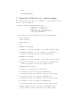
The coupling has been tested for an example in [4], where the length of a
recirculation bubble behind a backward facing step has been controlled by insufflation and suction at the edge of the step, see Fig. 1. This User Manual contains
complementary information to [4] by providing details about the practical implementation of the specific flow control problem, with the goal of facilitating
the use of the Featflow-Matlab coupling for other control problems.
2
Getting and installing Featflow’s Pp3d-Ke with
Matlab-interface
The installation procedure is only considered for Linux/Unix operation systems.
However, Featflow and Matlab can successfully work on Windows platforms,
1
control
recirculation zone
shear layer
reattachment length
Figure 1: Flow over a backward facing step (see [2])
the basic concepts regarding their communication through a Matlab-engine remain the same, but their joined installation under Windows was not approbated
in practice yet. The installation of Navier-Stokes solver with k − ε turbulence
model Pp3d-Ke with Matlab interface is done in the following steps:
1. Be sure that Matlab is installed. Any Matlab version with the appropriately working Fortran Engine- and Fortan MX-Functions can be used.
For assurance take Matlab of version 6.0 or later.
2. Be sure that Featflow is installed. Featflow is an open-source CFD
code and can be downloaded at http://www.featflow.de. All the required
details concerning its installation and usage are described in [6] and [3].
3. For the preparation of the geometry mesh it is suggested to use DeViSoR Grid3 program. DeViSoR Grid3 is a user-friendly preprocessing
tool, written in Java. DeViSoR itself and a user manual concerning its
installation are available at http://www.featflow.de.
4. The Pp3d-Ke module with Matlab-interface (Pp3d-Ke-matlab) is not
currently available in the standard Featflow package and therefore needs
to be downloaded separately. In order to obtain its latest version, please
contact directly Michael Schmidt or Andriy Sokolov.
5. Suppose that Matlab is installed into the directory /myapp/Matlab/ and
Featflow with Pp3d-Ke-matlab module is installed into the directory
/myapp/Featflow/applications/pp3dke matlab/
(a) Copy your Matlab m-file (say its name is ”myController.m”) into
/myapp/Matlab/myController/
(b) Prescribe to the parameter ”matlab” (which is in Featflow data-file
/myapp/Featflow/applications/pp3dke matlab/#data/ke3d.dat)
a value ’/myapp/Matlab/myController/myController.m’
6. Choose among available Matlab libraries, located in
/myapp/Matlab/extern/lib/, a library, which fits to your platform and
set its directory path to the environmental variable LD LIBRARY PATH:
setenv LD LIBRARY PATH /myapp/Matlab/extern/lib/requiredLibDir
7. Compile Pp3d-Ke application (e.g. ”make -f myMake.m”).
2
8. Run Pp3d-Ke application (e.g. ”./pp3dke matlab myApp”, where ”myApp”
is an extension of the data files: ”pp3d.myApp” and ”ke3d.myApp”).
3
Test problem backward facing step
We present the basic structure of the coupling and recall the test problem from
[4].
General control problems
Considering flows, let v = v(t; x) with v = (vx , vy , vz )T ∈ R3 denote the timeaveraged velocity and p = p(t; x) ∈ R a time-averaged pressure, both defined on
a time-space domain (0, T ) × Ω with T > 0 and Ω ⊂ R3 . v and p are governed
by Reynolds-averaged Navier-Stokes equations (RANS), see e.g. [4].
Dealing with flow control problems, we assume that we are able to influence
the flow in Ω by manipulating the Dirichlet boundary conditions in a subset
Γctrl ⊂ Γwall , i.e.
v(t; x(c) ) = u(t; x(c) )
for (t; x(c) ) ∈ (0, T ) × Γctrl ,
with a control or input function u(t; x). We assume further that we can observe
or measure the fluid’s velocity field and/or pressure field in subsets Ωmeas ⊂ Ω
and/or Γmeas ⊂ Γ, i.e. we know the observation or output function
y = y(t, x(m) ),
y = (v, p),
where (t, x(m) ) ∈ (0, T ) × (Ωmeas ∪ Γmeas ).
A (feedback) controller u(t, x(c) ) = f (t, y(s ≤ t, x(m) )) can then be used for
the calculation of appropriate controls u, possibly on the basis of current and
former observations y, in order to achieve some control objective.
While flow calculations are carried out in a performant manner with Featflow’s Pp3d-Ke program, the controller can be comfortably implemented in
Matlab.
The interaction between Pp3d-Ke and Matlab was realized with the help
of the Matlab Engine (function engOpen), which operates by running in the
background as an independent process. This offers several advantages: under
UNIX, the Matlab engine can run on the user’s machine, or on any other UNIX
machine on the user’s network, including those of a different architecture. Thus,
the user can implement a user interface on his/her workstation and perform the
computations on a faster machine located elsewhere on a network (see Matlab
Help).
The Matlab-controller part is realized as an m-file myController.m. During the simulation the Pp3d-Ke code calls this Matlab function at every time
step. The transaction phase consists of three stages: receiving the required
data (geometry, velocity, pressure) from the output domain Γmeas , execution of
myController.m and calculation of a control u = (ux , uy , uz ), setting v = u
as a Dirichlet boundary condition for velocity in the input domain Γctrl . So
myController.m has, in principle, the following interface:
(c)
(m,v)
˜ (xi ) = myController(tn , xj
v
3
(m,p)
, xk
(m,v)
˜ (xj
,v
(m,p)
), p˜(xk
)),
(m,v)
Here, tn is the current time, xj
(m,p)
, xk
are the coordinates of the velocity
(m,p)
(m,v)
˜ (xj
) and p˜(xk
) are the
and pressure nodes lying in Γmeas ∪ Ωmeas , and v
corresponding discrete velocity field and pressure field, respectively, all communicated by Featflow to Matlab. After the control is executed on the basis of
this information (and possibly of similar data computed at previous time steps),
(c)
(c)
˜ (xi ) with respect to xi ∈ R3 , the coordinates of
the discrete velocity field v
the velocity nodes lying in Γctrl , is communicated by Matlab to Featflow.
Controlling the flow over a backward facing step
As a specific test case, in [4] the flow over a step of dimensionless height h = 1 is
considered. The inlet section has the length 5h and the wake section the length
20h. The height as well as the width of the domain are 3h. We choose x, y and
z as coordinates for the downstream, the vertical and the spanwise direction,
respectively, see Fig. 2.
Γsym
25
Γin
3
2
y
h=1
z
x
Γwall
3
20
Γctrl
Ω meas
Γout
Γwall
Figure 2: The computational domain.
We assume that we can blow out and suck in fluid in an angle of 45 degree
in positive x-y-direction at a slot at the edge of the step of width 0.05h in the
x and y direction, i.e.
1
v(t; x, y, z) = √ (u(t), u(t), 0)T
2
on (0, T ) × Γctrl ,
where u(t) is a scalar control function that can be freely varied in time and
Γctrl = {(x, y, z) ∈ Γ : 4.95 ≤ x ≤ 5, 0.95 ≤ y ≤ 1, 0 < z < 3}. Note that the
implementation of distributed vector-valued controls v(t; x, y, z) = u(t; x, y, z)
is also possible.
The length of the recirculation zone is defined via the reattachment position
xr of the shear layer detaching at the edge of step. For each z, xr (t, z) is defined
by a zero wall shear stress τw (t; x, z) = 0, with
∂vx
τw (t; x, z) = η
|(t;x,y=0,z) ,
(1)
∂y
where η denotes the viscosity [2]. We will determine τw (t; x, z) by measuring vx (t; x, y, z) in the domain Ωmeas = {(x, y, z) : 5 < x < 20, 0 < y <
0.125, 0 < z < 3} and define a scalar reattachment length xr (t) by averaging
τw (t; x, z) in spanwise direction.
4
In the example, the following boundary conditions have been prescribed.
v(t; x, y, z) = v∞ = (1, 0, 0)T
∂v
(t; x, y, z) = 0
∂z
∂v
(t; x, y, z) = 0
∂n
v(t; x, y, z) = 0
on Γin
(inhom. Dirichlet),
(2a)
on Γout
(hom. Neumann),
(2b)
on Γsym ,
(symmetry),
(2c)
on Γwall ,
(no slip).
(2d)
In [4], a controller has been developed with the goal of choosing the input u(t)
such that the output y(t) = xr (t) tracks a given reference reattachment length
xref (t). This controller has been designed in form of a time-discrete linear
time-invariant dynamical system
xn+1 = Axn + Bun ,
yn = Cxn + Dun ,
n = 1, 2, . . .
with matrices A ∈ Rn,n , B ∈ Rn,1 , C ∈ R1, n and D ∈ R1,1 . Here xn ∈ Rn
denotes the state, un ∈ R the input and yn ∈ R the output at time tn = nδt
with time step size or sampling rate δt. Figure 3 shows the performance of the
controller in a numerical experiment. In the next sections, we describe how this
control concept can be realized by means of the Featflow-Matlab coupling.
9
xref(t)
xr(t)
8
7
6
5
0
0.1
0.2
0.3
0.4
0.5
0.6
0.7
0.4
0.5
0.6
0.7
time t
4
u(t)
2
0
−2
−4
0
0.1
0.2
0.3
time t
Figure 3: Tracking response of the closed-loop system and the applied control.
5
4
Setting of related parameters in Featflow
Specification of geometry
Using mesh creation tools like DeViSoRGrid [1], which can be downloaded
from the Featflow-homepage, 2D meshes can be created. In order to obtain
3D meshes, a 2D mesh can be extended to a 3D mesh e.g. by means of the
Fortran subroutine tr2to3, for more information on mesh generation see e.g. [6].
The resulting mesh and parameter files "myMesh.tri" and "myMesh.prm" are
usually stored in the directory "../applications/pp3dke$\_$matlab/#adc".
In [4], a backward facing step as in Fig. 2 resulted in a mesh as in Fig. 4
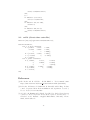
Figure 4: Mesh on multigrid level 3 (22848 elements)
Parameters in ”../applications/pp3dke matlab/as features.f90”
The Fortran file as features.f90 is the basic module organizing the communication between Featflow and Matlab. In particular, it contains a subroutine
which is called after every time step. Here the output data is read from Featflow, the Matlab engine is used to execute the m-file myController.m, the
output data from myController.m is transferred to Featflow.
!**********************************
!** Property: USER
!** This is a user-Matlab call subroutine (called from the MAIN)
!**********************************
SUBROUTINE useMatlab(itnsM, timensM)
INTEGER :: itnsM
REAL(KIND=rk) timensM
print *,’’
print *,’useMatlab is under progress ...’
!read the FEATFLOW data (from m-output domain)
CALL readOutputData()
!execute the matlab function "myController(itns,time,numOutFaces,v_x,v_y,v_z)"
CALL useMatlabSubroutine(itnsM, timensM)
!write data to the FEATFLOW (to m-input domain)
CALL writeInputData()
print *,’useMatlab finished its work.’
6
print *,’’
END SUBROUTINE
Parameters in ”../applications/pp3dke matlab/#data/pp3d.myApp”
We present selected lines from the file "pp3d.myApp" and comment on some of
the parameters defined there.
======================================================================
File for input data for pp3d
======================================================================
unit numbers and file names on /FILES/:
----------------------------------------------0
IMESH (0=FEAT-parametrization,1=OMEGA)
0
IRMESH (0=create mesh,>0=read (>1: formatted))
’#adc/myMesh.prm’ CPARM (name of parametrization file)
’#adc/myMesh.tri’ CMESH (name of coarse mesh file)
’#data/myApp.out’ CFILE (name of protocol file)
1
ISTART (0=ZERO,1=NLMAX,2=NLMAX-1,- =formatted)
’#data/myStart’
CSTART (name of start solution file)
1
ISOL
(0=no,1=unformatted,-1=formatted)
’#data/myEnd’
CSOL
(name of final solution file)
-----------------------------------------------CPARM and CMESH contain the position of the mesh files. If CSTART is set to 1,
the simulation starts with an initial value stored in the file "myStart". This file
name is specified in the parameter CSTART. If CSTART is set to 0, the simulation
starts with a zero initial value. If ISOL is set to 1, the flow field at the end point
of the simulation is stored in the file "myEnd", which can be specified in CSOL.
The file "myEnd" can e.g. be used as an initial value for a succeeding simulation.
3.0D4
1D9
1.0D0
1D-3
0
2.0D0
3
100.5D0
RE
NITNS
THETA
TSTEP
IFRSTP
DTGMV
IGMV
TIMEMX
(Viscosity parmeter 1/NU)
(number of macro time steps)
(parameter for one step scheme)
(start time step size)
(0=one step scheme,1=fractional step)
(time difference for GMV output)
(level for GMV-output)
(max. absolute time)
The simulation stops if either the maximal number of timesteps NITNS or the
end time TIMEMX is reached. If the simulation starts with an initial value coming
from a prior simulation, the time specified in "myStart" is automatically taken
as start time. The time step size is specified in TSTEP. The fractional step
scheme does not work in the present implementation, set therefore IFRSTP to
0. Featflow saves regularly snap shots of the flow field, readable by the
postprocessing software GMV. DTGMV specifies the time interval between two
snap shots, IGMV the multigrid level, from which the flow field data is taken.
7
Specification of input and output domains
Boundary conditions, like (2), are defined in the file indat3d.f, see [6] for
details. The actuator and sensor positions are specified in the subroutine NEUDAT
of indat3d.f. Again, we present selected lines from indat3d.f.
Considering the example in [4], we have Dirichlet control on the boundary
segment
Γctrl = {(x, y, z) ∈ Γ : 4.95 ≤ x ≤ 5, 0.95 ≤ y ≤ 1, 0 < z < 3}.
This is implemented by means of following lines of FORTRAN code.
************************************************************************
LOGICAL FUNCTION M_INPT(PX,PY,PZ)
*
*
This is the user-defined function:
*
prescribes the boundaries of the m-input domain
*
PX,PY,PZ - the center of the element
************************************************************************
IMPLICIT DOUBLE PRECISION(A,C-H,O-U,W-Z),LOGICAL(B)
C
M_INPT=.FALSE.
C
C
in-Matlab domain
if((PX.GE.4.95D0).AND.(PX.LE.5D0).AND.(PY.GE.0.95D0)
*
.AND.(PY.LE.1D0))then
M_INPT=.TRUE.
endif
C
C
END FUNCTION M_INPT
In [4], the velocity is measured in the domain
Ωmeas = {(x, y, z) : 5 < x < 20,
0 < y < 0.125,
0 < z < 3}.
The corresponding implementation reads:
************************************************************************
LOGICAL FUNCTION M_OUT(PX,PY,PZ)
*
*
This is the user-defined function:
*
prescribes the boundaries of the m-output domain
*
PX,PY,PZ - the center of the element
************************************************************************
IMPLICIT DOUBLE PRECISION(A,C-H,O-U,W-Z),LOGICAL(B)
C
M_OUT=.FALSE.
C
if((PX.GE.5.0D0).AND.(PX.LE.20.0D0).AND.(PY.GT.0.0D0)
*
.AND.(PY.LE.0.125D0))then
M_OUT=.TRUE.
8
endif
C
END FUNCTION M_OUT
5
Structure of the Matlab control routine
The Matlab m-file myController.m realizing the control law must have an
interface of the following form.
function velArr0=myController(itns,time,...
numInFaces,coordInFaces,...
numOutFaces,coordOutFaces,...
numOutElements,coordOutElements,...
v_x,v_y,v_z,presArr)
Here the input and output parameters have the following meaning.
• itns (integer)
iteration time step
• time (double)
time
• numInFaces (integer)
the number of nodes (the midpoints of faces) in the m-input domain
• coordInFaces (double, vector of length 3 x numInFaces)
coordinates of the midpoints of faces in the m-input domain
• numOutFaces (integer)
the number of nodes (the midpoints of faces) in the m-output domain
• coordOutFaces (double, vector of length 3 x numOutFaces)
coordinates of midpoints of faces in the m-output domain
• numOutElements (integer)
the number of elements in the m-output domain
• v_x (double, vector of length 3 x numOutFaces)
vx values in midpoints of faces, which are in the m-output domain
• v_y (double, vector of length 3 x numOutFaces)
vy values in midpoints of faces, which are in the m-output domain
• v_z (double, vector of length 3 x numOutFaces)
vz values in midpoints of faces, which are in the m-output domain
• presArr (double, vector of length 3 x numOutElements)
pressure values in elements, which are in the m-output domain
9
• velArr0 (double, vector of length 3 x numInFaces)
velocity values for the m-input domain.
As an example we present the body of the controller program which has
been used in [4]. Some parameters are initialiazed in the following lines.
% reset output array
velArr0=zeros(1,3*numInFaces);
% User-defined switches and parameters
ctrlChoice
= 2;
CtrlLawPath
= ’.../myController/’;
Since the Matlab engine is called in each time step, Matlab data has to be
written to a mat-file if it shall be available in succeeding time steps. The following lines of code are a data preprocessing step. Input/Output data from prior
time steps that is needed by the controller is loaded from the file iodata.mat.
The physical coordinates and the corresponding output data are sorted with
respect to their physical position.
%======================================================
% preprocess data
%======================================================
% loading of old iodata
if itns==1,
n_iodata=0;
else
load([CtrlLaw_path,’iodata’]);
n_iodata=size(iodata,2);
end;
% Reshape Coordinates
Xout=reshape(coordOutFaces,numOutFaces,3);
% change to "reattachment x-coordinates" (=x-x_step)
Xout(:,1)=Xout(:,1)-5*ones(numOutFaces,1);
% Sort Output Coordinates and Values according to x-coordinate
[Xout,SortIndex]=sortrows(Xout,[1 2 3]);
v_x=v_x(SortIndex)’;
We now illustrate how easily the reattachment length can be calculated in
the Matlab-file myController.m on the basis of the flow data Xout and v_x
communicated by Featflow. Approximating
τw (x, 0, z) ≈ η
vx (x, y, z) − vx (x, 0, z)
y
and in view of the no-slip boundary conditions at the bottom wall, i.e. vx (x, 0, z) =
0, we obtain for every entry in v_x an approximation of the wall shear stress in
the corresponding (x, z)-position,
10
tau_w=v_x./Xout(:,2)
Note that we are only interested in the zeros of τw and can thus neglect η. Now
there are several possibilities to extract from tau_w the reattachment length
xr . A simple possibility is to average over all tau_w -values with identical
x-position and then to define xr as a zero of the corresponding averaged τ¯w (x)distribution. Since the differing y-positions of the node points corresponding to
v_x may influence the quality of the approximations τ¯w (x), it may be reasonable
to take a polynomial fitting of τ¯w (x) instead of τ¯w (x) itself.
%=======================================================
% Soft sensor : extracting reattachment length
%=======================================================
%Calculate wall shear stress approximations
tau_w=v_x./Xout(:,2); % difference quotient (v_x(y=y0)-v_x(y=0))/y0
%Calculate tau_w(x) by averaging in y and z direction
xindex=1;j=0; xtol=0.001;
while xindex<=numOutFaces,
j=j+1;
x(j)=Xout(xindex,1);
%Find all coordinates with x=x(j) using tolerance xtol
zIndices=find(Xout(:,1)>=x(j)-xtol&Xout(:,1)<=x(j)+xtol);
xmean(j)=mean(tau_w(zIndices));
xindex=zIndices(end)+1;
end;
% Fit tau_w by polynomial
% and take largest real zero in [0,15] as rettachment length x_r
tau_poly=polyfit(x,xmean,7);
tau_wf=polyval(tau_poly,x);
tau_roots=roots(tau_poly);
j=1;tau_rroots=5;
for i=1:length(tau_roots),
if (imag(tau_roots(i))==0)&&(real(tau_roots(i))>0)&&(real(tau_roots(i)<15)),
tau_rroots(j)=real(tau_roots(i));
j=j+1;
end;
end;
x_r=max(tau_rroots);
The control is calculated and applied by means of the following lines of code.
If a closed loop control is chosen, the matrices A, B, C and D of the discrete-time
controller are defined in an m-file getcontroller.m, see Appendix A.2. The
reference trajectory xref (t), cf. Fig 3, is also defined in an m-file, see Appendix
A.1. It is assumed that the sampling rate for which the controller is designed
corresponds to the time step of the Featflow simulation.
%=======================================================
% Define Control-Law
11
%=======================================================
u=0;
switch ctrlChoice,
case 1, % no control
case 2, % open loop: e.g. constant control over a time interval,
starttime
= 0.05;
endtime
= 0.55;
if and(time>=starttime,time<endtime),
u = 0.6;
end;
case 3. % closed loop control
% define closed loop controller as discrete lin. state space model
% (designed for sampling rate dt=0.001)
[A,B,C,D]=getcontroller(2);
if itns==1,
xold=zeros(size(B));% take controller initial state = 0
else
load([CtrlLaw_path,’xold’]);% load controller state from last time step
end;
e=xref(time)-x_r;% define deviation from reference
% calculate control
xnew=A*xold+B*e;
u=C*xnew+D*e;
xold=xnew; save([CtrlLaw_path,’xold’],’xold’);% save controller state
end
% Apply control: blowing and sucking at slot with alpha degree
alpha=45; %normally =45
velArr0(1,[1:numInFaces])=cos(alpha*pi/180)*u*ones(1,numInFaces);
velArr0(1,[numInFaces+1:2*numInFaces])=sin(alpha*pi/180)*u*ones(1,numInFaces);
Since the controller needs output data from the previous time step, the
necessary data is stored in a datafile iodata.mat.
%=======================================================
% Data postprocessing: Saving
%=======================================================
iodata(1,n_iodata+1)=time;
iodata(2,n_iodata+1)=u;
iodata(3,n_iodata+1)=x_r;
iodata(4,n_iodata+1)=xref(time);
save([CtrlLaw_path,’iodata’],’iodata’);
12
The current τw (x) distribution and the evolution of the reattachment length
and of the control over time are plotted online in a Matlab window, cf. Fig
5, such that the functioning of the control concept can be evaluated already
during the simulation.
Figure 5: A screenshot of the Matlab window showing the current τw (x) distribution, and the reattachment length and control evolution.
%=======================================================
% Data postprocessing: Plots
%=======================================================
%Plot tau_w distribution and sign-changes
titletext=sprintf(’tau_w(x) at t=%3.4f (itns=%3.0f)’,time,itns);
subplot(3,1,1)
plot(x,xmean,’-’,x,tau_wf,’g-’,x_r,[0],’ro’);
title(titletext,’FontWeight’, ’bold’, ’FontSize’, 12);
xlabel(’x’);
ylabel(’\tau_w’);
% plot output over time
subplot(3,1,2)
hold on
plot(iodata(1,:),iodata(4,:),’g-’); %desired recirculation length
plot(iodata(1,:),iodata(3,:),’b-’); %real recirculation length
titletext=sprintf(’reatt. length over time ...
[currently: x_{ref}-x_r=%3.4f , x_r=%3.4f]’,xref(time)-x_r,x_r);
13
title(titletext,’FontWeight’, ’bold’, ’FontSize’, 12);
xlabel(’t’);
ylabel(’x_r(t)’);
% plot input over time
subplot(3,1,3)
plot(iodata(1,:),iodata(2,:));
title(’control over time’,’FontWeight’, ’bold’, ’FontSize’, 12);
xlabel(’t’);
ylabel(’u(t)’);
%====================== return to FEATFLOW!
6
Running a flow calculation with control
In order to run a simulation, first compile an executable code by means of
make -f ke3d.matlab_athlinux
after adapting the make-file ke3d.matlab athlinux to your needs. Then you
start a Featflow simulation including the Matlab coupling by means of
../ke3d myApp
A
A.1
Appendix
m-file (reference reattachment length)
function out=xref(t);
xr0=6.2102; % uncontrolled reattachment length
refchoice=2;
out=xr0; %default value
%--if and(t>=0.05,t<0.15),
out=xr0-1;
end;
%--if and(t>=0.25,t<0.35),
out=xr0+1.5;
end;
%--if and(t>=0.45,t<0.451),
out=-(t-0.45)*200+xr0;
end;
if and(t>=0.451,t<0.549),
out=xr0-2;
end;
if and(t>=0.549,t<0.55),
14
out=(t-0.549)*200+xr0-2;
end;
%--if and(t>=0.7,t<0.705),
out=-(t-0.7)*400+xr0;
end;
if and(t>=0.705,t<0.795),
out=xr0-2;
end;
if and(t>=0.795,t<0.8),
out=(t-0.795)*400+xr0-2;
end;
A.2
m-file (dicrete-time controller)
function [A,B,C,D]=getcontroller(modelChoice);
switch modelChoice,
case 1, % slow controller
A = [0.8917
0.5000
0.0379;
-0.0384
0.8917
0.0427;
0
0
0.9999];
B = [0.3024;
0.3403;
0.2060];
C = [-1.3878,
0,
-0.2060];
D = -1.6417;
case 2, %fast controller
A =[ 0.6849,
1.0000,
-0.0558;
0,
0.9999,
-0.0648;
0,
0,
0.9473];
B =[ 0.4993;
0.5795;
0.2394];
C =[-0.7649,
0,
0.2394];
D = -2.1418;
end;
References
[1] Ch. Becker and D. G¨
oddeke. DeViSoRGrid 2. User’s manual, 2002.
http://www.featflow.de/feast hp/devisormain.html (10.02.2006).
[2] R. Becker, M. Garwon, C. Gutknecht, G. B¨arwolff, and R. King. Robust
control of separated shear flows in simulation and experiment. Journal of
Process Control, 15:691–700, 2005.
[3] A. Sokolov D. Kuzmin and S. Turek. Pp3d-Ke User Guide, Finite element
software for the incompressible Navier-Stokes equations including the k − ǫ
turbulence model. Institute of Applied Mathematics, University of Dortmund, www.featflow.de.
15
[4] L. Henning, D. Kuzmin, V. Mehrmann, M. Schmidt, A. Sokolov, and
S. Turek. Flow Control on the basis of a Featflow-Matlab Coupling. In Active Flow Control 2006, Berlin, Germany, September 27 to 29, 2006. Berlin:
Springer. Notes on Numerical Fluid Mechanics and Multidisciplinary Design
(NNFM). 2006. accepted for publication.
[5] The MathWorks, Inc., Cochituate Place, 24 Prime Park Way, Natick, Mass,
01760. Matlab Version 7.0.4.352 (R14), 2005.
[6] S. Turek and Ch. Becker. FEATFLOW. Finite element software for the incompressible Navier-Stokes equations. User manual, release 1.1, Universit¨
at
Heidelberg, 1998.
16