Download RiboSort User Manual

RiboSort User Manual
´ Scallan
Una
April 20, 2007
1
Introduction
RiboSort is an R package for automated data preparation and exploratory analysis of microbial community profiles. It facilitates the sorting of many automatic
sequencer generated profiles at once, thus eliminating the tedious and time consuming operation of manually manipulating and sorting profiles.
This document illustrates a sample session using the RiboSort package. It
goes through loading data, running RiboSort to sort the data, and manipulating
results for preliminary statistical analysis. We assume a basic knowledge of R,
and thus advise familiarization with Appendix 1: Getting Started in R, if this
is your first encounter with the R programming environment.
To begin, start R, then load the RiboSort package:
> library(RiboSort)
2
Data Retrieval
RiboSort facilitates the direct input of data produced by two automatic sequencers, the Applied Biosystems (ABI) Gene Mapper and the Beckman Coulter
CEQ 8000 Genetic Analysis System. Data can also be read from other formats
if you reformat it manually into RiboSort’s defined standard profile (see section 2.1). We welcome contributions for routines for importing data from other
formats.
2.1
Standard Profile
A standard profile defined for the RiboSort package contains two columns. The
first column lists fragments detected in the sample in increasing order. Their
associated relative abundances, represented by peak heights in the sequencer
output, are listed in a second column. An example of a standard profile is
illustrated in Figure 1.
2.2
Applied Biosystems 3130XL (GeneMapper)
The ABI 3130XL sequencer and its associated GeneMapper version 4.0 software
allow data to be exported in a wide variety of formats. Two of these formats are
compatible with RiboSort. The first contains a single community profile which
we denote ABIsingle, and the second can contain multiple profiles, denoted
1
Figure 1: RiboSort’s standard profile format.
ABImultiple. Instructions for retrieval of these formats using the GeneMapper
software are now described.
ABIsingle
• Once logged into the GeneMapper software, select File → Open project
from the top menu. Highlight the desired project and click on Open. Set
tablesettings to AFLP default.
• Proceed by highlighting the sample to be exported. Click on the Display
Plot icon in the top toolbar. In the plot window that opens, set plot
settings to sizing, and subsequently select File → Export table. Save the
text file under its sample name in the desired location.
• An example of such a file is illustrated in Figure 2.
Figure 2: An ABIsingle text file.
ABImultiple
• Once logged into the GeneMapper software, select File → Open from the
top menu. Highlight the desired project and click on Open. Set tablesettings to AFLP default.
• Open the Genotypes tab and take note of the maximum allele number
detected in the set of samples. From the top menu, select Tools → GeneMapper Manager. Open the Report Settings tab and enter the project
name into the space provided. The maximum allele number should be
entered into the Number of Alleles box.
• In the Genotype tab of the Available Columns box, highlight the fields
to be included in your output (these are sample name, all sizes and all
2
heights) and click on the arrow pointing right toward the Selected Columns
box. Click on OK.
• Back in the GeneMapper window, highlight the samples you wish to export, or if all samples are to be included in the output file, enter Edit →
Select all.
• On the top menu, enter Analysis → Report Manager. In the report manager window that opens, there is a drop-down menu entitled Report Settings. In this menu, select the project you just created.
• On the top menu, select Edit → Flip Table. Then select File → Export. . .
and save the output text file under its project name in the desired location.
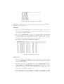
An example of such a file is illustrated in Figure 3.
Figure 3: An ABImultiple text file.
• One final step is required to make this output compatible with RiboSort.
Open the text file, say projectname.txt, in Excel. Select File → Save as. . .
and save the file as a comma separated file, projectname.csv. This file is
now ready to be used in the RiboSort package. An example of such a file
is illustrated in Figure 4.
Figure 4: An ABImultiple comma separated file.
Note: Ensure that no empty profiles are exported to the text file created by
GeneMapper. An empty profile containing no sequencer detections will make
the text file incompatible with RiboSort and will produce an error if submitted.
3
2.3
Beckman Coulter CEQ 8000 Genetic Analysis System
The CEQ 8000 control and analysis software allows data to be exported in a
wide variety of formats. To retrieve analysis results in a RiboSort compatible
format, follow the guidelines given below.
• Open the Genetic Analysis System software and from the top menu in the
sequencer program, select File → Export Results.
• Choose the sample to be exported and proceed, leaving all default settings
in place. On the Elements page, ensure that the Header and Results Data
options are not ticked. This action will create a RiboSort compatible text
file.
• An example of such a file is illustrated in Figure 5.
Figure 5: An extract from a Beckman text file.
3
Data Loading
To load data for use with the RiboSort package, copy any data files to be sorted
into your current working directory (see Appendix 1 for explanation of the
working directory). The RiboSort package contains a number of R functions.
The behaviour of these functions can be altered by changing optional arguments.
The most important function in this package is RiboSort itself. This is the
function to which you submit your data. In order to submit more than one file
at a time to the RiboSort function, a data vector containing the list of filenames
needs to be created. We now demonstrate how to create a data vector called
mydata in R.
> mydata = c("sample1.txt", "sample2.txt", "sample3.txt", "'sample4.txt")
There is a limit of 1000 characters allowed for filenames within the parentheses
of a data vector. When there are many files to be processed and the character
limit in mydata is reached, successive files can be stored in additional datasets
mydata2, mydata3, etc. All datasets can then be combined into a total data
vector as shown in the example below.
>
>
>
>
mydata1 =
mydata2 =
mydata3 =
allmydata
c("sample1.txt", "sample2.txt", ..., "sample74.txt")
c("sample75.txt", "sample76.txt", ..., "sample149.txt")
c("sample150.txt", "sample151.txt")
= c(mydata1, mydata2, mydata3)
4
In this example the data vector that should be submitted to the RiboSort
function is allmydata. Note that with the exception of ABImultiple files, which
are comma separated (.csv ), all other data files will be text files (.txt ). It is also
important to note that all files listed in a data vector must be of the same format
(either Standard, ABIsingle, ABImultiple or Beckman).
4
The RiboSort Function
Depending on the size and number of data files, and the speed of your computer,
running RiboSort may be slow. There are seven arguments to the function
RiboSort. Each of these arguments works as a interactive tool, allowing the
user to personalize the method of classification carried out. See the help file
?RiboSort for more information. To run the examples in the help file, all the
demonstration datafiles (including thirteen .txt files and one .csv file) provided
in the RiboSort package must be copied to your current working directory.
The complete RiboSort function is shown below, with each of the seven
arguments set to their default values.
> x = RiboSort(data, dataformat = "standard", dye = "B", output = "proportions",
+
zerorows = FALSE, repeats = 1, mergerepeats = "none")
We now proceed to describe the purpose of each argument and the available
options for them.
data A data vector listing the filenames of each profile to be sorted. Recall
that each file listed must be stored in the current working directory to be
detectable by R.
dataformat The format of profiles listed in data. This must be one of "standard", "abisingle", "abimultiple" or "beckman".
dye An indicator code identifying the dye that corresponds to the primer used.
The argument dye only comes into effect when dataformat is "abisingle" or "beckman". The ABIsingle files generally just have a single letter
dye indicator, eg. "B", "R", "Y", etc., whereas Beckman sequencer files
usually have dye indicators of the form "D1", "D4", etc.
output Specifies whether the R object produced by RiboSort will contain abundances (as given in the original profiles) or the relative proportions of
abundance in each profile. output must be one of "abundances" or "proportions". Statistical analysis is usually performed on the relative proportions of abundance, thus the default is "proportions".
zerorows A logical argument (can only take values TRUE or FALSE) indicating
whether zerorows are to be kept in the output or not. A zerorow refers to
a ribotype not detected in any of the profiles supplied. When FALSE, the
default, zerorows are deleted from the output. When TRUE, the zerorows
remain in the output.
repeats The number of repeat profiles taken from each sample. If repeats is
greater than 1, profiles listed in data must be in an order, such that all
repeats from a particular sample are listed adjacent to one another. For
5
example, if there were two repeats and five samples, Samp1repeat1 would
be listed first followed by Samp1repeat2, Samp2repeat1, Samp2repeat2,
etc.
The number of repeats must be constant for all samples. If this is not the
case, submit repeats = 1 to obtain a sorted output of all profiles, and
proceed to manually merge repeat profiles.
mergerepeats The method of merging a number of repeat profiles from the
same sample into a single composite profile for that sample. mergerepeats
must be one of "none", "presentinall", "presentintwo" or "presentinone".
The "none" option indicates that profiles are not to be merged. To merge
repeat profiles taken from the same sample into a single composite profile,
there are three methods. The first of these, "presentinall", specifies that
the composite profile only contains ribotypes detected in all of the repeat
profiles. Thus, ribotypes present in less than all of the repeat profiles, are
not included in the final composite profile.
The second method, "presentintwo", specifies that the composite profile
only contain ribotypes detected in at least two of the repeat profiles. Finally, the "presentinone" method indicates that all ribotypes detected,
even those only present in one repeat profile, are included in the composite
profile. This is the default option.
Following the execution of any of the three merging methods, the composite profile produced for a sample will be named according to the first
repeat profile listed in data for that sample.
Composite profile abundances are determined by averaging the relative
proportions present in repeat profiles.
When repeats is greater than 1 and mergerepeats="none", no profile
merging will occur and all profiles submitted will be present in the output.
5
Managing and Saving Output
Each time the RiboSort function is run, four Excel files are created and stored
in the current working directory. Ribotypes Output.xls contains assigned and
aligned detections while Abundances Output.xls contain their respective abundances. Proportions Output.xls is a simple manipulation of Abundances Output.xls that displays the relative proportions of abundance in each profile. Information File.xls details changes made to the data by the RiboSort function.
Note that Excel files of these four names cannot be open while RiboSort is
running.
To simplify interpretation of the contents, these four files require some slight
editing. Instructions to carry out the recommended adjustments are now described.
To edit Ribotypes Output.xls, Abundances Output.xls or Proportions Output.xls:
• Open the file in Excel. Select Column A by clicking on the letter A in the
top left-hand corner of the spreadsheet.
6
• From the top menu, enter Data → Text-to-columns → tick Delimited →
Next → tick Tab & Space → Next → Finish.
• Once files have been adjusted in this manner, they are referred to as edited
output files. Save all edited output files as Excel spreadsheets. To avoid
overwriting output files with a later execution of RiboSort, it is advised
at this time to rename your files appropriately.
• The first column in each of the edited files contains a list of integers covering the range of ribotypes detected in the sample set. Depending on
which of the three files you are dealing with, the remaining columns display ribotype sequencer detections, abundances or abundance proportions
for each sample.
To edit Information File.xls:
• Open the file in Excel.
• Use the text-to-columns function (as above) to first separate Column A
from the rest of the data (tick Other after Delimited and enter a colon in
the space provided).
• Proceed to use the text-to-columns function again, this time on Column
B to separate the remainder of the data (tick Space after Delimited).
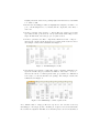
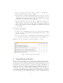
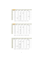
Examples of the four edited files are shown in Figures 6, 7, 8 and 9.
Figure 6: An edited Information File.xls.
6
Using RiboSort Results
A RiboSort object (that is the object created in R by running the RiboSort function) is a matrix with columns representing samples and rows representing ribotypes (putative species). Although an Excel file containing this matrix is created
by the RiboSort function (Abundances Output.xls if output="abundances" or
Proportions Output.xls if output="proportions"), the function also stores the
matrix as an R object to facilitate further analysis in the R environment.
The RiboSort package has two functions samplesMDS and speciesMDS that
produce multi-dimensional scalling (MDS) plots of samples and species respectively. These functions enable simple and quick production of multi-dimensional
7
Figure 7: An edited Ribotypes Output.xls file.
Figure 8: An edited Abundances Output.xls file.
Figure 9: An edited Proportions Output.xls file.
8
scaling plots. They each take four arguments that work as a interactive tools,
allowing the user to personalize the plots. A choice of dissimilarities is available,
as well as the option to specify the desired type of multi-dimensional scaling.
See the help file ?sampleMDS for more information.
Note that at least three samples are required to produce a two-dimensional
plot. The complete functions are demonstrated below, with each argument set
to its default value.
> samplesMDS(x, dissimilarity = "euclidean", type = "non-metric",
+
labels = TRUE)
> speciesMDS(x, dissimilarity = "euclidean", type = "non-metric",
+
labels = TRUE)
We now proceed to describe the purpose of each argument and their associated
options.
x A numeric matrix, dataframe or a RiboSort object, ie. an object created by
the RiboSort function.
dissimilarity The distance measure to be used computing dissimilarities between samples or species. This must be one of "euclidean", "maximum",
"manhattan", "canberra", "binary" or "minkowski". Any unambiguous
substring can be given.
type The type of Multi-dimensional Scaling to be used. This must be one of
"classical", "sammon" or "non-metric", the default.
labels An logical argument indicating whether or not labels are to be included
on the MDS plot. When FALSE, labels are omitted.
When deciding upon a dissimilarity measure, the following description (available
in the help file ?dist) of options may aid your choice. Available dissimilarity
measures are (written for two vectors x and y):
euclidean Usual square distance between the two vectors.
maximum Maximum distance between two components of x and y.
manhattan Absolute distance between the two vectors.
canberra sum(|xi − yi |/|xi + yi |). Terms with zero numerator and denominator
are omitted from the sum and treated as if the values were missing.
binary The vectors are regarded as binary bits, so non-zero elements are ’on’
and zero elements are ’off’. The distance is the proportion of bits in which
only one is on amongst those in which at least one is on.
minkowski The p norm, the pth root of the sum of the pth powers of the
differences of the components.
When choosing which type of multi-dimensional scaling to use, the following
elaboration on the options available may aid your choice.
classical Classical multi-dimensional scaling of a data matrix. Also known
as principal coordinates analysis.
9
sammon Sammon’s non-linear mapping, also known as metric least squares multidimensional scaling.
non-metric Kruskal’s form of non-metric multidimensional scaling.
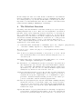
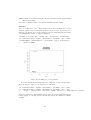
Example:
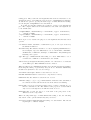
Let x be a RiboSort object. This example shows how an MDS plot for four
samples, generated by the Beckman Coulter sequencer, is produced. The plot,
illustrated in Figure 10, is created using non-metric multi-dimensional scaling
on a dissimilarity matrix of euclidean distances.
> mydata = c("beck1.txt", "beck2.txt", "beck3.txt", "beck4.txt")
> x = RiboSort(data = mydata, dataformat = "beckman", dye = "D4")
> samplesMDS(x, dissimilarity = "euclidean", type = "non-metric",
+
labels = TRUE)
Figure 10: An MDS plot of four samples.
Note that arguments left unspecified are evaluated at their default values.
The following two lines of code are therefore equivalent.
> x = RiboSort(data = mydata, dataformat = "beckman", dye = "D4")
> x = RiboSort(data = mydata, dataformat = "beckman", dye = "D4",
+
output = "proportions", zerorows = FALSE, repeats = 1, mergerepeats = "none")
For a more interactive and less limited approach to producing multi-dimensional
scaling graphs, see the help files for the following functions: cmdscale, sammon,
isoMDS.
10
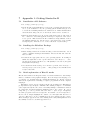
7
Appendix 1: Getting Started in R
7.1
Installation of R Software
• Go to http://cran.r-project.org/.
• In the Download and Install R box, select the operating system appropriate to your workstation. If your operating system is Windows, proceed
to follow the remaining instructions outlined below. Linux and MacOS X
users should at this point, choose the latest version of R to download.
• Enter the base subdirectory. To download the latest version of R, click on
R-. . . -win32.exe. Save this application and upon completion of the download, open it. This activates the R for Windows Setup Wizard. Follow
the Wizard instructions. On the select components page, leave default
settings in place. Tick the box to create a shortcut on your desktop.
7.2
Intalling the RiboSort Package
• Go to http://cran.r-project.org/.
• Enter Packages under the Software heading on the left hand side. Scroll
down to Available Packages and Bundles. Browse the list and enter the
RiboSort link.
• Download the appropriate file for your operating system. If working in
Windows, right-click on the .zip file and select Save Target as. . . Save
the file in the library subdirectory of R (usually located at C:/Program
Files/R/R-2.4.1/library).
• Now start R from the desktop icon. On the top menu, enter Packages →
Install packages from local zip files. . . The package is now installed and
ready for use in R.
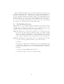
7.3
Brief explanation of How R works
The R environment is an integrated suite of software facilities for data manipulation, calculation and graphical display. R is an interpreted language, not
a compiled one, meaning that all commands submitted are directly executed
without the requirement of building a complete program like in most computer
languages.
When R is opened on your computer, the R console will appear. This issues a
prompt when it expects input commands. The default prompt is >. Commands
can be input directly into the console. Generally, multiple commands are written
in a script file and then submitted simultaneously to the console. To open a
script file, go to the top menu and select File → Open Script. Frequently,
an entire program is saved in a script file. To submit code in a script file to
the R console, simply highlight the desired code and right-click Run line or
selection. Errors in code are communicated via error messages in the console.
These messages appear in blue font, making them easily distinguishable from
successfully executed code which appears in red.
11
Help is available through R via the top menu. The Manuals (in PDF) option
provides seven manuals that comprehensively document R’s functionality. In
particular, An Introduction to R introduces the language and explains how to
use R for statistical analysis and graphics. All R objects (including functions,
datasets, packages, etc.) have associated documentation files. These can be
accessed via the R console by typing a question mark followed by the name of
the object. For example, submit ?sum to your R console. Note the vast index
of documented objects that appears on the left hand side.
7.4
The Working Directory
All files that are to be imported (used) by R must be stored in the current
working directory. Files created by R are also stored in this directory. It is
recommended to use different working directories for different projects you are
working on. There are two ways to set up a working directory:
Method 1 Right-click on the R shortcut displayed on your desktop and enter
Properties. The Start In field contains the path to the current working
directory. To change working directory, simply change the path so that it
refers to the desired folder. All files to be used by R must be stored in this
folder, and any output files created by R will also be stored in this folder.
Method 2 Establish the current working directory by submitting the following
code. To do this type getwd() in the R console and press enter.
> getwd()
To change the working directory submit the code below inserting the path
to the folder you wish to use as your working directory within the inverted
commas. Forward slashes as opposed to backslashes must be used in the
path name.
> setwd("C:/uscallan/myRiboSortfolder")
To confirm the change of directory, resubmit getwd().
12