Download Contact Angle Measuring Instrument User Manual

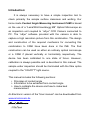
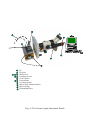
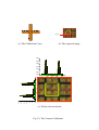
Home made
Contact Angle Measuring Instrument
User Manual
By
Ahmed Abdelmonem
27/02/2008
Introduction:
It is always necessary to have a simple inspection tool to
check primarily the sample surface cleanness and wetting. Our
home made Contact Angle Measuring Instrument CAMI is based
on the use of a “Leica/Wild Heerbrugg M8” Optical Microscope as
an inspection unit coupled to “uEye” CCD Camera connected to
PC. The “uEye” software provided with the camera is able to
capture a high resolution picture from this combination. The design
and construction of the required mechanics for converting this
combination to CAMI have been done in the INE. The final
construction can be used as either an ordinary optical microscope
or a CAMI if placed vertically or horizontally respectively. The
device has been calibrated to one state of focus. However,
calibration is always possible and is described in this manual. The
sample under inspection should be illuminated with the fibre optics
coupled to the “SCHOTT” light source.
This manual includes the following sections:
1.
2.
3.
Principles of contact angle
Information to be extracted from contact angle
How to calibrate the device and how to make best
measurement
An Electronic version of the “User manual” can be downloaded from
www.amamonem.de
Ahmed Abdelmonem
27/02/2008
7/02/2008
13
2
14
1
3
5
9
12
4
10
8
11
6
7
1
2
3
4
5
6
7
8
9 10
11
12
13
14
PC
Eyepiece
Water-level
Levelling screws
CCD Camera
Focus Knobs
Levelling mount
Micro-stage (Sample holder)
Micro syringe
Eliminating fibres
Fig (1): The Contact Angle Instrument Sketch
1 Principles of Contact Angle:
Geometrically, contact angle is defined as the angle formed by a liquid at the three
phase boundary where a liquid (L), vapour (V) and solid (S) intersect. It is a quantitative
measure of the wetting of a solid by a liquid (hydrophilicity / hydrophobicity), surface
tension, adhesion, cleanliness, and biocompatibility. The shape of a liquid droplet on a flat
horizontal sold surface is determined by the Young-Laplace equation:
∆p = γ∇.nˆ
= 2γH
 1
1 

= γ  +
 R1 R2 
where
∆p : The pressure difference across the interface
γ : The surface tension.
nˆ : The unit vector normal to the surface.
H : The mean curvature.
R1 , R2 : The radii of curvature of the two principle
curvatures.
R2
R1
Fig(2)
N.B.
In our case, we consider the drop as a part of a sphere, hence R1 = R2 .
At thermodynamic equilibrium between the three phases (L, V and S), the chemical
potential in the three phases should be equal. The interfacial energies can be related to
the contact angle through either,
1. Young Equation:
γ SV − γ SL − γ LV cos θ c = 0
where;
γ SV : The solid-vapor interfacial energy.
γ SL : The solid-liquid interfacial energy.
γ LV : The liquid-vapor energy (the surface tension)
θ c : The experimentally measured contact angle.
γ LV
γ SL
θc
γ SV
Fig(3)
or
2. Young-Dupré equation:
γ LV (1 + cos θ c ) = ∆WSLV
where,
∆WSLV is the adhesion energy per unit area between the solid and liquid surfaces when in
the vapor medium.
2 Information to be extracted from contact angle
Contact angle is rich of information depending on the given parameteres of the
sample under study.
*
* www.firsttenangstroms.com
3 System alignment, measurement and calibration:
3.1
Alignment
1. Adjust the microscope and the sample holder horizontally using the levelling screws (6
and 7) and the water-levels (3, 4, and 5).
2. Place the sample on the sample holder (12) and use the Illuminating fibres to get best
view of the sample edge from the Eyepiece (2)
3. Run the camera software and confirm the horizontality of the
camera (8) by focusing the view on the sample holder edge
(8). Lose the side screw which tights the camera to rotate it if
required. The focus can be adjusted using the Focus Knobs (9
and 10). It is recommended that you adjust the focus using
Fig(4)
(10) and keeping (9) on 50 if you want to use the default
calibration (section 3.3 ).
Tip: Whenever the horizon can not be brought into sharp focus, tilt the microscope about 3° using (6).
3.2
Measurement
4. Adjust the Syringe tip (13) right over the sample.
5. Use (10), (11) and the micrometer screw of the sample holder (12) to get the Syringe
tip into the focus.
6. Carefully generate a small hanging droplet of water at the tip of the syringe.
7. Elevate the sample slightly and carefully until it touches the water droplet. The droplet
will drop onto the surface.
8. Adjust the focus again until you get sharp edges of the half
sphere formed by the droplet. It is better to use the same
droplet volume (using the graduated syringe) in each
experiment if you are interested in comparing results. It is also
recommended that the droplet be as small as possible.
9. Acquire a picture using the camera software, save it and then
edit it with any graphic software (Corel designer is
recommended).
Fig(5)
10. Roughly, you can decide whether the surface is hydrophilic or hydrophobic when the
contact angle is either acute- or wide-angle respectively.
11. In the Corel Designer you can define two lines; one is parallel
to the base and the other is the tangent to the half sphere
border; then measure the angle between them.
12. If your study requires measuring the dimensions of the droplet
on the surface, then you need to calibrate the Camera.
Fig(6)
3.3
Calibration
The camera is already calibrated to the state where the focus is obtained by knob
(10) when knob (9) is at 50. In this case the dimensions will be related to the number of
pixels measured by the graphic software as follows:
x: 1mm~505px
y: 1mm~530px
This means that the resolution of the camera of 1280px X 1024px corresponds to 2.55mm
X 1.93mm. (The obtained picture should be resized to these dimensions)
To calibrate the camera do the following steps:
1. Stick a small millimetre paper on the sample holder edge. It is recommended to use
the Standard Calibration Cross SCC, figure (7a) which can be printed from
www.amamonem.de
2. Follow the steps 1-3 in (section 3.1) and acquire a good resolution image from the
SCC, figure (7b).
3. Using suitable software (Winspec is recommended), you can transfer this obtained
2D image to 3D (x,y,Intensity), and deconvolute it to I(x) and I(y) as shown in Figure
(7c). To get an exact calibration, you can fit the intensity peaks to Lorentz bands
using the Origin software for example. The difference between central positions of
two successive peaks in pixels corresponds to 1mm.
1.0 mm
(c) The Calibration Cross
(b) The captured image
0.030
0.025
0.020
0.015
0.010
0.005
0.000
200
400
600
800
0.000
0.005
0.010
0.015
0.020
0.025
0.030
0
200
400
600
800
px
0
(c) Picture deconvolution
Fig (7): The Camera Calibration
px
Acknowledgment
All the acknowledgments to Dr. Geckeis, Dr. Klenze, Dr. Hauser,
Dr. Lützenkirchen and Mr. Büchner for their cooperation in building
this device.