Download 1 Spectrum Lab User's Manual Contents

1 Spectrum Lab User's Manual
This „document“ is just a collection of all HTML files from Spectrum Lab's built-in help system.
They were simply combined in a master document in OpenOffice, by means of 'including' the html
pages as sub-documents.
Unfortunately, the links between these sub-documents (which were once HTML pages heavily
linking to each other, and to the 'index.htm' page) get broken in the OO document. This is the reason
why all those helpful links don't work in the PDF you are currently reading.
If you have a solution (i.e. how to convince OpenOffice to get the hyperlinks working again,
without having to edit zillions of links manually), please let me know.
Also, if you know how to prevent OpenOffice from turning the chapter numbers (from multiple
HTML files "included" by the master document) into a complete mess - see 'Contents' below..
Contents
1
Spectrum Lab User's Manual..........................................................................................................1
2.1.6 Installation and directory structure .................................................................................5
2.1.7 Setting up the soundcard (or other input devices) ..........................................................6
2.1.8 How to check and avoid an unwanted bypass between the soundcard's Line-In and
Line-Out .....................................................................................................................................6
Some notes on Creative Lab's "Audidy 2" (tested with Audigy 2 ZS) and how to avoid
Line-In -> Line-Out bypass ("feedthrough") .........................................................................7
2.1.9 Some notes on various other soundcards .......................................................................9
2.1.10 Quickstart for QRSS (very slow Morse code viewer) ................................................. 9
2.1.11 Running multiple instances of the program ............................................................... 11
2.1.12 Configuration data files ..............................................................................................12
3 Controls in the main window ...................................................................................................... 14
3.1 Main Window ...................................................................................................................... 14
3.1.1.1 File ........................................................................................................................14
Start/Stop .........................................................................................................................14
Options ............................................................................................................................ 15
Quick Settings ................................................................................................................. 15
3.1.1.2 View/Windows ..................................................................................................... 15
3.1.1.3 Help ...................................................................................................................... 15
3.1.2 Built-in "Quick Settings" (in the main menu) ..............................................................16
3.2 Spectrum Display .................................................................................................................17
3.3 Control Elements in the main window ................................................................................ 17
3.3.1 Tabbed display control panel ........................................................................................17
Frequency control panel (in SpecLab's main window) ........................................................18
3.3.2 Time Axis ..................................................................................................................... 19
3.3.3 Cursor Position Display ............................................................................................... 20
3.3.3.1 Fixing the cursor on a certain frequency ..............................................................21
3.3.4 Color Palette Control ................................................................................................... 21
3.3.5 Progress Indicator/Stop Button ....................................................................................21
3.3.6 Programmable buttons ................................................................................................. 22
3.4 Controls on the bottom of the main window ....................................................................... 23
3.4.1 The Spectrum Buffer Overwiew (in the bottom control bar) .......................................24
3.4.2 Navigation buttons to scroll through the spectrogram buffer ...................................... 24
4 Spectrum Displays .......................................................................................................................25
4.1 Spectrum Graph ...................................................................................................................25
4.2 Waterfall Display (aka Spectrogram) ...................................................................................26
4.2.1 Visual AGC (for the spectrogram colour palette) ........................................................ 28
4.2.2 Amplitude Bar (alongside the spectrogram display) ....................................................29
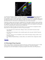
4.3 3D Spectrum Display ...........................................................................................................29
4.4 Reassigned Spectrogram ......................................................................................................30
4.5 Correlogram .........................................................................................................................31
4.6 Frequency Scale ...................................................................................................................32
4.6.1.1 Popup menu of the main frequency scale..............................................................33
4.6.1.2 Adjusting the visible part of the frequency scale ................................................. 34
4.6.1.3 Adding or subtracting a user-defineable frequency offset (for the display) .........34
4.7 One or two channels for the spectrum display .....................................................................34
4.8 Spectrum Averaging (Overview) ......................................................................................... 35
4.8.1 The "Second Spectrogram" .......................................................................................... 36
5 Spectrum Lab Configuration Dialog ........................................................................................... 38
5.1.1 Transceiver Interface Settings.......................................................................................39
5.2 System Settings.....................................................................................................................40
5.2.1 Memory and spectrum file buffers................................................................................40
5.2.2 Audio Server Settings....................................................................................................41
5.2.2.1 Timezone............................................................................................................... 41
5.2.2.2 Geographic Location............................................................................................. 41
5.2.3 Timer Calibration.......................................................................................................... 41
5.2.4 Clock Source for timestamps:.......................................................................................41
5.2.5 Filenames and Directories.............................................................................................42
5.2.6 Adding a special driver for other audio input devices...................................................46
5.2.7 The Audio I/O Libraries................................................................................................46
5.2.8 Using in_AudioIO.dll to stream audio into Winamp.................................................... 48
5.2.9 Using in_AudioIO.dll to stream audio from the first instance of Spectrum Lab to other
instances....................................................................................................................................48
5.2.10 Using a Winrad-compatible ExtIO-DLL for input......................................................49
5.2.10.1 FiFi SDR..............................................................................................................50
5.2.11 Output resampling.......................................................................................................51
5.2.12 Soundcards with "slightly different" sample rates for the input (ADC) and output
(DAC)........................................................................................................................................52
5.2.13 Multiple soundcards in one system.............................................................................53
5.2.14 Unexpected aliasing at 48 kSamples/second on a Windows 7 system........................53
5.3 Audio File Servers and Clients............................................................................................. 53
5.3.1 PIC-based A/D converter for the serial port..................................................................55
5.3.2 Sending and receiving audio through WM_COPYDATA messages............................ 55
5.3.3 Sending and receiving audio through a local network..................................................55
5.3.4 The Winamp-to-SpecLab output plugin........................................................................56
5.3.5 Sending audio from SpecLab to Winamp..................................................................... 56
5.3.6 Loading Winamp plugins into SpecLab........................................................................56
5.4 FFT settings.......................................................................................................................... 57
5.4.1 Spectrum Display Settings............................................................................................59
6
7
8
9
5.4.2 Spectrum Buffer Settings..............................................................................................64
5.5 Display Colour Settings........................................................................................................65
5.6 Frequency Marker Settings...................................................................................................66
5.6.1 Functions (and -commands) to access frequency markers through the interpreter.......67
5.6.2 Frequency marker types................................................................................................67
5.6.3 Radio- vs Baseband frequencies................................................................................... 68
5.7 Audio File Settings (formerly 'Wave File Settings')............................................................. 68
5.8 Amplitude Calibration...........................................................................................................69
5.9 Settings and Configuration Files...........................................................................................70
Radio Station Frequency List ...................................................................................................... 71
6.1.1 Loading and displaying a frequency list ...................................................................... 71
Spectrum Lab Circuit Components ............................................................................................. 72
7.1 Component Window.............................................................................................................72
7.1.1.1 Chaining of both processing branches (since 2004-07) ....................................... 74
7.2 Monitor Scopes.....................................................................................................................74
7.2.1 Universal Trigger Block ...............................................................................................75
7.2.2 Counter / Timer (pulse- or event counter, operating in the time domain) ....................76
7.2.3 Input Preprocessor ........................................................................................................77
7.3 Test Signal Generator............................................................................................................78
7.4 Programmable Audio Filter.................................................................................................. 78
7.5 Frequency Converter ("mixer")............................................................................................ 78
7.6 Audio input and output......................................................................................................... 79
7.6.1 Output- and "cross coupling" amplifiers ......................................................................80
7.7 Spectrum analyser.................................................................................................................80
7.8 DSP Black Boxes .................................................................................................................80
7.8.1.1 Signal processing sequence (in each DSP Blackbox) .......................................... 81
7.8.2 Adder or multiplier (to combine two input channels in a DSP blackbox) ...................81
7.8.3 Bandpass Filter (in a DSP blackbox) ........................................................................... 82
7.8.4 Delay line in a DSP blackbox ...................................................................................... 82
7.8.5 Advanced hum filter in a DSP blackbox ......................................................................83
7.8.6 Hard Limiter in a DSP blackbox ..................................................................................84
7.8.7 Noise Blanker in a DSP blackbox ................................................................................84
7.8.8 DC Reject / DC measurement (in a DSP blackbox) .....................................................85
7.8.9 Modulators and Demodulators in a DSP blackbox ......................................................85
7.8.9.1 Wideband FM reception .......................................................................................86
7.8.10 Automatic Gain Control (in the DSP blackboxes) .....................................................86
7.8.11 Chirp Filter (in the DSP blackboxes) .........................................................................87
7.9 Sampling Rate- and Frequency Offset Calibrator ...............................................................87
7.10 Interpreter commands for the test circuit ...........................................................................87
Spectrum Lab's "watch window" .................................................................................................89
8.1 The watch list .......................................................................................................................89
8.2 The History Plotter ...............................................................................................................91
Mouse-tracking readout function .........................................................................................92
8.3 Plotter Settings .....................................................................................................................92
8.4 Interpreter functions to control the watch window and it's plotter ...................................... 96
Digital Filters ...............................................................................................................................98
9.1 1. FFT filter ..........................................................................................................................98
9.2 1.1 Controls and Options for the FFT-based filter ...............................................................99
1.2 Controlling the filter via SL's main frequency scale..........................................................102
9.3 1.3 FFT-based frequency conversion ("pitch shift")...........................................................103
9.4
9.5
1.4 FFT-basedUSB / LSB conversion ("frequency inversion")..........................................104
1.5 FFT-based autonotch.....................................................................................................104
9.5.1.1 1.5.1 Options for the FFT-based automatic notch filter...................................... 104
9.6 1.6 I/Q processing with the FFT-filter................................................................................ 105
1.6.1 FFT-based filter as I/Q modulator (to generate SSB signals)................................... 106
9.6.1 1.6.1 FFT-based filter as I/Q modulator (to generate SSB signals)........................... 106
9.7 1.7 FFT Filter Plugins.........................................................................................................107
9.8 2. Filter Implementation..................................................................................................... 107
9.8.1 Starting and stopping the filter ...................................................................................108
9.8.2 Testing the filter on your PC ...................................................................................... 109
9.9 DSP Literature ................................................................................................................... 109
9.10 Interpreter commands for the digital filters ..................................................................... 109
9.10.1.1 A few "tricks" using the color palette editor... ..................................................113
Spectrum Lab Installation and Program Start
Contents
1.
2.
3.
4.
5.
6.
7.
8.
System Requirements
Installation and directory structure
Setting up the soundcard
Quickstart for QRSS (very slow Morse code viewer)
Program start with command line arguments
Configuration data files
Running multiple instances of the program
Creating shortcuts for different configurations
Special topics:
1. How to avoid an unwanted audio bypass from the soundcard's input to output (Line-In to LineOut)
2. How complicated this can be when using Creative Lab's Audigy 2 ;-)
3. How to install and run Spectrum Lab under Linux / Wine
4. How to use SL with software-defined radios like SDR-IQ or PERSEUS
See also: Spectrum Lab's main index
System Requirements
You will need the following to use "SpecLab":
- a PC with Win95, Win98, WinME, Win2k, WinXP, Windows 7, or Linux+Wine
- a soundcard with an audio input resolution of 16 bits
- a color graphics mode with at least 800*600 pixels with 256 colors
(a graphics mode with higher resolution and "true color" is preferred, and even required under WinXP
and any later version of Windows)
back to top
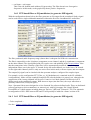
2.1.6 Installation and directory structure
To install the program on your PC, follow the instructions of the installation program. If the program
requires special DLLs, they will be installed automatically. An uninstaller will be configured too, so you
can remove this software easily if you don't need it any longer.
The default directory for the installation was once C:\Spectrum, but in the days of windows Vista and
Windows 7 this may have been changed - the installer will suggest to place the program somewhere in the
'Programs' directory, whereever that may be on your machine. If not absolutely necessary, don't change
this because some of the example settings contain absolute path names. Some subdirectories will also be
created by the installer:
..\Data\
default directory for data files, like logged data files from long-term observations etc.
Because Spectrum Lab must have write-access permission for this directoy, the installer may have
to place it somewhere else (very annoying, but that's what windows Vista wants..).
To simplify the task of 'finding' this (and other) writeable directories, the installer will write a short
text file which contains the DIRECTORY PATHS to all 'writeable' directories ... thanks Microsoft
for changing this over and over ... the ugly details are here ("data folders").
..\Export\
contains some export file definitions and example user settings. Beginning with Windows Vista and
Windows 7, the directory path for this folder also had to be moved somewhere else (because any
Spectrum Lab Manual
5 / 113
folder under 'Programs' doesn't have write permission by default) - more details here ("data
folders").
..\Goodies\
contains additional information and special files. More info in a readme-file in the subdirectory.
..\Html\
contains the online help system.
After successful installation, you may optimize some parameters for your requirements. You should (but
you don't have to).....
Adjust your soundcard settings for proper audio levels
Check the level of the soundcard input with the input monitor
Define the difference between UTC("GMT") and your local timezone
Verify everything in the Configuration-Dialog
Adjust the amount of memory used for buffering
Test the digital filter on your PC
Check if there is an unwanted audio bypass from the soundcard's input to its output, which spoils
the software-DSP
• If you intend to use Spectrum Lab with the SDR-IQ (by RFSPACE), read this document .
• Users of PERSEUS (a software defined radio by Microtelecom in Italy), read this .
•
•
•
•
•
•
•
back to top
2.1.7 Setting up the soundcard (or other input devices)
By default, Spectrum Lab uses the windows multimedia system for audio input and -output. Details on
setting up the soundcard properly are here (in a separate file).
If your soundcard (or similar audio device) supports ASIO, look here because ASIO works better with
some cards (especially at sampling rates above 48 kHz and resolutions above 16 bit).
To use SL with SDR-IQ or SDR-14 (by RFSPACE), install SpectraVue too. This will install the necessary
USB drivers (by FTDI) which are not included in SL.
To use SL with PERSEUS (by Microtelecom s.r.l), install the Perseus software, and the WinUSB drivers
for your particular OS. More details here .
To process samples from your own A/D converter, consider using the file-based audio input, or send the
audio stream towards SpecLab via UDP or TCP/IP (UDP is best suited for simple microcontrollers with
Ethernet interface).
back to top
2.1.8 How to check and avoid an unwanted bypass between the soundcard's Line-In
and Line-Out
For real-time signal processing with SpecLab's internal DSP functions, an analog audio signal must get
into the PC somehow, and to make to processed signal audible it must get out of the PC so we can listen
to it with headphones or external speakers. This should be no big problem nowadays, because modern
cards support "full duplex" operation, which means their analog-to-digital converter (ADC) and digitalto-analog converter (DAC) can run simultaneously. So we can use the DAC to produce test signals, and
the ADC to analyze a different signal at the same time. Or we can use the ADC to digitize a signal, run it
through some digital processing algorithm, and convert it back into an analog signal in real-time.
Sounds easy, because our brand-new soundcard has two audio jacks for this purpose, labelled "Line-In"
Spectrum Lab Manual
6 / 113
and "Line-Out". So what's the point ?
Often things are not that easy. There are a lot of different signal paths inside a soundcard, different
sources and destinations, and very different (and incompatible) ways to connect all these. The default
settings of many cards are not suitable for us, because they feed the signal which enters the card through
the "Line-In" port directly to the "Line-Out" port, for whatever reason. This is not very helpful here,
because we only want the PROCESSED signal to appear at the "Line-Out" port. We also do not want the
signal at "Line-Out" to be fed back into the analog-to-digital converter, because this may cause heavy
feedback or heavy oscillation (making the stereo speakers jump through the living room !). Too bad !
Both situations must be avoided. In other words:
Be prepared to spend a few hours playing with your soundcard's own "volume control panel" (or
whatever the manufacturer called it), until you managed that the audio input (from the "line-in" jack)
only(!!) goes into the A/D converter, and the card's audio output (the "line-out" jack) is only fed from the
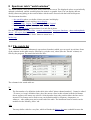
D/A converter, without annoying bypass. The standard audio volume control program (SoundVol32.exe)
is often all we have. If can be launched from SpecLab's Options menu, to show the settings for
"recording" (analog-to-digital conversion) and "replay" (digital-to-analog conversion). Just a few points
to be aware of:
• On the "Recording Gain Control" screen ("Aufnahmesteuerung" in German) , only select the
"Line-In" signal as recording source, or mute all other sources for recording. Unfortunately
sometimes there is no "Line-In" as recording source, but an "Analog Mix" which makes it more
complicated (as for the Audigy, see below).
• On the "Playback Volume Control" screen ("Wiedergabe", or "W-gabestrg." as CL likes to call it),
only select "Wave" as playback source, or mute all the others. "Wave" often means the D/A
converter.
• On some cards like the Audigy 2 (you have to enable "Line-In" also on the playback volume
control screen, otherwise it won't record !!), the cure is not simple but possible then .. see below !
• Also enable the "Master Volume" on the playback panel, otherwise you won't hear anything from
the speakers.
• Sometimes all these problems are gone if you use an ASIO driver instead of a standard multimedia
audio device !
Some notes on Creative Lab's "Audidy 2" (tested with Audigy 2 ZS) and how to avoid
Line-In -> Line-Out bypass ("feedthrough")
In May 2004 the author played with his new Soundblaster 2 ZS (by Creative Labs), because this card
really supports analog sampling at 96 kHz (unlike some previous cards... but that's another story). Some
first impressions...
• After installing the drivers by CL, the onboard audio device disappeared from the system control most likely because there would have been an I/O address- and interrupt- conflict with the new
card. Unfortunately this makes it impossible to use both cards simultaneously (which was planned
to have ultimate separation between a "test signal" produced by one card, which should be fed to
the input of the other card then). To get two cards working, one of the cards must be an USB card
(like the Extigy, which does ***NOT*** support analog sampling at 96 kHz btw).
• Feeding a test tone from an external audio generator into the "Line-In" jack, running it through
SL's software DSP chain, and sending the processed output to the soundcard's analog output
("Line-Out 1") showed the well-known feedthrough-problem, which means the audio from the
Line-In port also went straight to the Line-Out port. More on this below...
• Simultaneous recording (A/D conversion) and playing (D/A conversion) at 96 kHz worked fine
right from the start, without having to modify the soundcard interface code (I use standard
multimedia subsystem calls to access the soundcard).
Unlike many other soundcards, there is no extra mute-control for the "Line-In" input for the speaker
outputs (which they call "Quelle" in german). Even the good old SoundVol32.exe (part of windows) does
NOT show a "Line-In" volume slider or select/mute control, but only an "Analog Mix" control. To make a
Spectrum Lab Manual
7 / 113
long story shorter, I tried a lot with SoundVol32.exe and CL's "Surround Mixer" (SurMixer.exe) but
always had this annoying bypass. Some web research revealed this solution, found in a newsgroup on the
Creative Labs website when searching for "Audigy Line-In recording with Wave playback".
The question was:
> I have only Mic/Analog Mixer selector in Windows2000 record selector panel.
> Moreover, I can only record signal from LineIn only if I also select LineIn in Playback mixer.
> Does Audigy really has such kind of limitation?
An answer from "Sicabol":
> [...]
> You have to create a new EAX effect. Open the EAX Control Panel (in AudioHQ),
> click the Source tab. You will see a listbox with all the different sources which are playing now...
> Desactivate the sources you don't want to play by setting 0% to their original sound.
> I advise you to save your new setting.
> If you want to have the default settings back (after your recording),
> click "Reinitialisate the mixer" in the Creative taskbar.
> [...]
This answer was also very helpful for my application. But still, with the utilities from Creative it's
complicated enough (I wonder if it's so unusual to let only the output from the D/A converter go to the
output and nothing else ? .. anyway). You need the "EAX Console", which is only on the CDROM which
comes with the Audigy (not just the drivers). Here is the step-by-step procedure, which I used on a
German PC:
• In the task bar: "Start"..."Programme"..."Creative"..."Soundblaster Audigy 2 ZS"..."Creative
AudioHQ".
A window opens, with an icon "EAX-Steuerung" (EAX Control). Double-click this icon.
• Select the "Master" tab in the EAX control panel / AudioHQ, where you...
• set "Audio Effects" to "Benutzerdefiniert" (user defined), and type a name like "SpecLab" in the
right field on the top, so you can export the settings you made as a file later,
• on the "Master" tab, move the gain sliders for "Orignalklang" to 100%, but "Nachhall" and "Chor"
(chorus) to minimum (0 %).
• on the "Source" tab ("Quelle" in German), first select "Quelle=Wave", set the slider
"Originalklang" to 100%, and all others ("Nachhall", "Chor") to 0%
• then, again on the "Source" tab (Quelle), select "Quelle=Analog Mix(Line/CD/Aux/TAD/PC"
(instead of "Wave"), and pull all three sliders to zero ("Originalklang", "Nachhall", "Chor"). The
names may be a bit cryptic, but at least this seemed to do the trick !
• Finally save the settings (click on the floppy icon, which should be enabled now), and/or export
them as a file so you can easily switch back to them later. I saved the settings as
"Audigy2_EAX_settings_for_SpecLab.AUP", to know what the file is for ;-)
Gone through all this ? Start SpecLab again, feed a signal into the Audigy's line-input. From SpecLab's
main menu, select "Option"..."Volume control for RECORD". This opens the standard volume control
program (which belongs to windows, not SpecLab, and not Creative Labs). Only the "Analog Mix" must
be active as recording source. Because of the "EAX Effect" configured above, the "Analog Mix" is only
the analog input (line-in) but no other fancy stuff. You should now see the spectrum of the input signal in
the waterfall and/or spectrum graph, but not hear that signal (which you feed to the line-input) in the
speakers. Next, connect the test signal generator to the output (in SL's "Components"-window), and turn
the generator on to produce an audible sine wave. You should hear only the tone from the test signal
generator in the speakers or headphones, but not see it in the spectrum display ! (otherwise, you still have
that unwanted internal connection between A/D- and D/A-converter, which drove me nuts for several
hours..). If you don't hear the test tone in the output, select "Options" in SL's main menu, and "Volume
control for PLAY". Make sure the output to "Wave" is enabled (not muted), but that is usually the case by
default.
Spectrum Lab Manual
8 / 113
2.1.9 Some notes on various other soundcards
(just a loose compilation of feedback from other Spectrum Lab users)
• Audio 2 ZS and poor ASIO drivers
Only runs at 48 kHz sampling rate; and -with a *different* ASIO driver- at 96 kHz. On my PC,
24-bit at 96 kHz sampling also worked well with the standard MME (multimedia) driver, while
other users reported that they needed to switch to ASIO to get their cards running at 96 kHz .
Strange, but no real surprise ;-)
• ESI Julia ("ESI Juli@")
The Julia is a moderately priced card (about 140 Euros in early 2006), capable of stereo 24-bit
sampling at 192 kHz sample rate. Successfully tested with Spectrum Lab since the integration of
ASIO support. The Julia has a reasonably flat response to 90kHz and drops about 3dB by 96k.
2.1.10Quickstart for QRSS (very slow Morse code viewer)
... has been moved to a separate file (qrss_quickstart.htm) ...
Program Start with Command Line Arguments
For special purposes, you can pass a command line to the program when starting it. This is required only
if you...
• want to have multiple instances of the program running at the same time, with each one using its
own configuration file;
• want to have multiple instances of the program running at the same time, with one of them passing
audio data (as master) to other instances (slaves).
• have a system with more than one soundcard, and you want to create desktop icons to start an
instance of Spectrum Lab which uses a certain card (instead of the first detected audio device);
• want to help me debug the program, especially if the program crashes on your system but not on
the author's ;-)
An overview of parameters which can be set through the command line is here.
If you only have a single soundcard on your system, or only need a single configuration, don't read any
further on this page. It may be getting complicated.
The general syntax to start Spectrum Lab with command line arguments is like this:
SpecLab.exe <Machine-Config> <User-Config> [ <"Main Window Title"> ]
There are also some command line switches (options) which will be explained later.
Without using command line arguments, all parameters are saved in an old style INI-file named
"SETTINGS.INI" in the current directory of the spectrum analyzer.
Usually, in this file both machine- and user-dependent data are saved.
If you want to have multiple instances of the program running at the time using different configurations,
can tell the program which configuration file shall be used instead of the default "SETTINGS.INI". If you
don't specify the name of the configuration file in the command line, the program uses "SETTINGS.INI"
for the first running instance, "SETTING2.INI" for the second and "SETTING3.INI" for any further
instance.
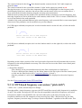
This can be achieved by passing one or more arguments to Spectrum Lab during program start. The first
character in each argument must be a lower case letter defining the type of the argument, followed by a
'='-character and the assigned value (e.g. a filename). Example:
Spectrum Lab Manual
9 / 113
SpecLab.exe m=Machine1.ini u=BandView.ini "t=Full Range Band View"
This will force Spectrum Lab to load the machine configuration data from "Machine1.ini" and the user
configuration data from "BandView.ini". The main window will have the title "Full Range Band View".
A more-or-less complete overview of command line parameters is in the next chapter.
Command line parameters prefixed with a slash, which are not listed below, will be passed on to
Spectrum Lab's internal command interpreter (see the "capture"-example below).
For special purposes, a few more command line options were implemented . There are:
• <filename.wav> Any string ending with the extension ".wav" is considered an audio file, which
will be played (instead of processing the input from the soundcard, or whatever used as standard
audio source).
• /si single-instance option. If the program is invoked with this switch, it will check if there is
another instance already running. Instead of launching a new instance, the rest of the command
line will then be sent automatically to the first (already running) instance, which will then evaluate
it a few milliseconds later. See examples below.
• /q tells the program to quit automatically when "finished" with playing an audio file. If it does not
play an audio file, it terminates itself immediately. Can be used together with the /si-option to fill
Spectrum Lab's internal playlist !
• /w tells the program to wait until the specified audio file has been played (or analysed), similar to
the /q option mentioned above. The rest of the command line (after the /w) will be parsed -or at
least "executed"- after finishing the file analysis. This allows, for example, to produce a screenshot
of the spectrogram *after* the file has been analysed (see examples below).
• /debug runs the program in "debug" mode. This creates a logfile as explained in the
troubleshooting guide.
• /noasio do not use ASIO drivers (only standard multimedia drivers).
Implemented 2011-08-09 when the program seemed to crash while trying to enumerate the
available ASIO drivers.
• /inst=N overrides the instance-detection, and instructs the program to run as the N-th instance
(N=1 to 6)
Some special examples:
• SpecLab.exe C:\Spectrum\SpecLab.exe /si
C:\Musik\Joe_Jackson\Classic_Collection\T03_Steppin_Out.wav /q
plays a certain wave file from the harddisk, and terminates itself when finished.
• SpecLab.exe /si /q
Checks if there is an instance of SL already running, terminates that first running instance (by
sending the /q command = quit to the first instance), and finally terminates itself. Can be used in a
batchfile to close down Spectrum Lab automatically.
• SpecLab.exe /si /capture
Sends the command to produce a screen capture of the waterfall (etc) to the first instance of
SpectrumLab. The same way, most interpreter commands can be invoked through the command
line !
• SpecLab.exe /si "t=Oops, what happend to my title ?"
Changes the window title of the first instance (which already ran before this command was
executed).
• SpecLab.exe test.wav /sp.print("Test") /w /capture("test.jpg") /q
Analyses the file "test.wav", prints a message into the spectrogram, waits until the analysis is
done, captures the (spectrogram-)screen as "test.jpg", and finally quits. Note the importance of the
sequence, especially the /w option.
See also: Communication with external programs, Audio Clients and Servers , Using a system with more
than one audio device , back to top
Spectrum Lab Manual
10 / 113
Overwiev of command line parameters
m= sets the name of the machine configuration file
u= sets the name of the user configuration file
t= sets a new title for the main windows
/si : option (switch) to send the rest of the command line to the first running instance. Explained here in
detail.
/q : quit option. Instructs the program to terminate itself when "finished", usually with playing a wave file
etc.
/w : wait option. Waits for file analysis, before the rest of the command line is executed. Details here .
/nomenu : hides the main menu (and the window borders) after launching the program. To restore the
main menu, press ESCAPE.
/inst=N : overrides the instance-detection, and instructs the program to run as the N-th instance (N=1 to 6)
.
/noasio : Do not use ASIO drivers (only standard multimedia drivers).
Implemented 2011-08-09 when the program seemed to crash while trying to enumerate the available
ASIO drivers.
/debug : For debugging purposes, specifiy the option /debug on the command line when launching
Spectrum Lab. The program will write a file named "debug_run_log.txt" into the current directory, which
may help me tracing bugs (answering questions like "how far did it get" - "where did it crash" - "why did
it load so slow" - etc ).
This proved to be a very helpful debugging aid, when the program crashed on certain machines, using a
certain windows version, a certain soundcard, etc. The contents of this debug log may look like this (just
an example, when the program terminated "normally") :
19:38:45.9 Logfile created, date 2012-10-15
19:38:45.9 checking instance...
19:38:45.9 Executable: c:\cbproj\SpecLab\SpecLab.exe
19:38:45.9 Compiled : Oct 15 2012
19:38:45.9 Data Files: c:\cbproj\SpecLab
19:38:45.9 init application...
... (many lines removed here) ...
19:38:55.7 Beginning to close ....
... (many lines removed here as well) ...
19:38:59.4 Deleting SPECTRUM objects
19:38:59.4 Deleting other buffers
19:38:59.4 FormClose done
19:38:59.4 Ok, all 85 dynamic memory blocks were freed.
19:38:59.4 Reached last termination step; closing logfile.
that the program closed "as it should")
(this message indicates
If you find any messages like "Serious Bug", "Fatal Error", "Allocation Error", "Application Error" etc in
that list, please let me know.
More details about running Spectrum Lab in 'debug' mode, and how/where to report bugs, is in the
'Troubleshooting' notes.
back to top
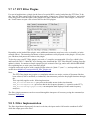
2.1.11 Running multiple instances of the program
If is possible to have more than one instance of Spectrum Lab running at the same time on a single PC (if
it's fast enough). Please don't try to let more than two instances run on one computer at the same time,
unless you have a really powerful CPU (i never tried it on my 266MHz-P2). Because a single soundcard
Spectrum Lab Manual
11 / 113
can only be opened by a single user, the second instance of Spectrum Lab will not be able to open the
same audio device as the first. See "Using a system with more than one audio device" in the description
of the configuration dialog.
If two instances of Spectrum Lab run side-by-side on the same PC, the program ensures that different
configuration files are used as described above.(at least for the first and second started instance). This
allows you to start two instances with the same shortcut icon on the desktop. Even different window
positions and sizes are saved in the configuration files. During program start, Spectrum Lab checks if it
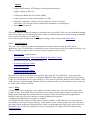
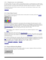
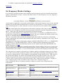
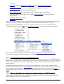
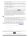
"already runs" in another instance. If so, the title of the 2nd instance's main window will display
something like this to avoid confusion:
The "[2]" in the window title also appears on some of the second instance's child windows.
Programmer's Information:
The detection of other instances uses mutexes. The first instance creates a mutex called "SpecLab1", the second a mutex
"SpecLab2". This is also a way to detect the presence of Spectrum Lab for other programs.
To bypass the instance-detection (which may be necessary in very rare cases), use the /inst=N command line option
(N=1...6) .
back to top
Creating shortcuts for different configurations
You can create a shortcut ICON with command line arguments / parameters. Right-Click on an empty
space of the desktop, then select "New..Shortcut (?? on a german PC: "Verknüpfung"), then find your way
to the directory where SpecLab is installed, and append the command line parameters (using hyphens).
The complete string should look like this (just an example, the path will be different on your machine !):
C:\Programs\SpecLab\SpecLab.exe "m=Machine1.ini" "u=BandView.ini" "t=My Title"
back to top
2.1.12Configuration data files
A lot(!) of configuration parameters are saved between to SpecLab sessions in old-fashioned INI files (not
in the registry ! ). One contains only machine-specific data (and should not be copied from one PC to
another), the other only stores application-specific data (and can safely be copied from one PC to another,
to run the program with the same settings there).
The machine configuration data contain:
•
•
•
•
the information which audio device (soundcard etc) shall be used, and how it is accessed
calibration tables for the audio device (true sample rates etc)
interface setup to control a transceiver (COM-port, control lines etc)
and possibly something more
The user configuration data contain:
•
•
•
•
screen setup
sample rate, frequency range, FFT resolution,
amplitude range
waterfall scroll rate, display colors, etc etc etc
back to top
Spectrum Lab Manual
12 / 113
See also: Spectrum Lab's main index
Spectrum Lab Manual
13 / 113
3 Controls in the main window
The main window of spectrum lab contains the most important controls and output of the spectrum
analyzer:
• Main Window with menu
• Predefined settings (in the "quick settings" menu)
• Spectrum Display (in separate document, with frequency scale, waterfall and/or spectrum graph)
• Time Axis
• Controls on the left side of the main window (with frequency control panel, various sliders,
progress button, programmable buttons, etc)
• Controls on the bottom of the main window (with the spectrum buffer overview)
• Cursor Position Display (readout cursor)
• Color Palette Control ("contrast and brightness" of the waterfall)
• Progress Indicator / Stop button
• Programmable buttons
Other functions may be implemented in other windows, which you can open from the "View" menu (in
SL's main menu).
See also: Spectrum Lab's main index.
3.1 Main Window
The main window contains the main menu, the spectrum display (on the right side) and -optionally- some
control elements on the left side, and some in the control bar on the bottom.
The main menu contains the following items:
3.1.1.1 File
• load settings, change directories and select file names for screen captures etc,
• configure screen capture, periodic and scheduled actions,
• view saved images (crude image viewer for BMP and JPG files),
• Select audio files for logging and for analysis.
Start/Stop
• Start and stop the audio processing thread,
• the spectrum analyzer,
• and other parts of the Spectrum Lab processing chain.
Spectrum Lab Manual
14 / 113
Options
• change Audio settings, FFT settings (for the spectrum analyzer),
• display settings, colours, etc,
• configure the Radio Direction Finder (RDF),
• change options for saving and analyzing wave files,
• launch the soundcard's volume control program for "record" and "play",
(check this if you run into trouble with unwanted feedback or audio bypass !)
• and some other specials..
Quick Settings
This menu allows to change all settings of Spectrum Lab very quickly. There are some predefined settings
in this menu, and some user-defineable entries which are initially empty. More about creating and adding
your own set of settings can be found here.
Some of the built-in configuration in the "Quick Settings" menu are described further below.
3.1.1.2 View/Windows
There are a lot of different windows in Spectrum Lab, many of them are only used for special
applications. The "View/Windows" menu allows you to switch to any of these sub-windows quickly, even
if they are hidden by other windows. Some of the sub-windows are listed here:
• Input monitor, output monitor,
• Test Signal Generator, Filter Control Window, Hum Filter Control,
• Spectrum Alert Function (control panel),
• Second Spectrogram window
• Time Domain Scope
• Watch List and Plot window
• Command Interpreter window
Hint: Windows which are already opened will be checked in the "View/Windows". You can quickly
switch between them, even if they are completely hidden by other windows on the desktop, by pressing
CTRL-F6 ("Switch between SL's open windows"). This works a bit like the Windows task switcher (ALTTAB), but only switches through Spectrum Lab's own windows. But a few SL windows may (or may not)
be visible in the windows task bar.
3.1.1.3 Help
Contains some topics of the help system and the inevitable "about"-box. The help system only works
properly if there is an HTML browser installed on your system which supports jumps to anchors in the
html documents through the command line. For example, if help about the spectrum graph shall be
displayed, SpecLab invokes the browser with the command line argument
"../html/specdisp.htm#spectrum_graph" (or similar).
The 'Help' menu also contains an item named 'Check for Update via Web Browser'. Use this function
occasionally. It will open a simple webpage, which checks if your version of Spectrum Lab is still up-todate, based on the program's compilation date, which is sent through the HTML query string. Please use
this function if you experience problems, before reporting bugs, as explained in the document about
'troubleshooting'.
Spectrum Lab Manual
15 / 113
back to top
3.1.2 Built-in "Quick Settings" (in the main menu)
Some typical configurations can be recalled from the "Quick Settigns" menu. In contrast to the userdefined settings (in the lower part of that menu), the following configurations are hard-coded in the
program - so they don't have to be loaded from an external configuration file. Most of these settings are
organized in categories (in the form of submenus), to avoid a bulky long top-level menu. The following
list may be incomplete since the program still keeps growing:
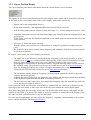
• Radio Equipment Tests
includes two-tone test (with calculation of 3rd-order intermodulation products), and a SINAD test
procedure.
• Slow Morse Reception
Used by radio amateurs to detect very weak, but coherent signals.
• Predefined Digimodes
Opens the digimode terminal, and shows a selection list for some of the implemented "digimodes"
(like PSK, Hell, transmission of Slow Morse Code, etc).
• Other Amateur Radio Modes
Optimizes the spectrum display to receive other amateur radio transmissions, without opening the
digimode terminal
• Image-cancelling DC receiver (with separate I/Q inputs)
Experiments with software-defined radio; more details here.
• Colour Direction Finder
Switches the waterfall into Radio Direction Finder-mode without affecting other settings.
• Natural Radio, Animal Voices
Spectrograms optimized for natural radio (sferics, "tweeks", and "whistlers"); Spectrograms to
examine human voice and animals in the audible spectrum, and a special mode to convert
ultrasonic bat calls into the audio range with a fast real-time spectrogram (requires a fast PC (at
least 1.7GHz) and a soundcard with at least 96 kHz sampling rate).
• Reassigned Spectrograms
can, under certain conditions, increase the time- and frequency resolution. The items in this
submenu are:
• Time- and frequency reassigned display
Switches from 'classic' waterfall to reassigned display mode, without changing anything
else. If this item is checked, the display already runs in 'reassigned spectrogram' mode.
• Frequency- but not time-reassigned display
Similar, but reassigns the short time fourier transforms along the frequency axis (not along
the time axis).
• Classic Spectrogram
Switches back to the classic (non-reassigned) spectrogram display.
• "Voices" (reassigned)
This is a sample application for a reassigned spectrogram, using a relatively fast, nonscrolling spectrogram with a logarithmic frequency scale.
Details about reassigned spectrograms are in a separate document; a comparison between a
Spectrum Lab Manual
16 / 113
'classic' spectrogram and a reassigned spectrogram is here .
• Restore all "factory" settings
Helpful if you got lost in all those settings, and cannot get the program working again. This
function restores most settings to the same state after the original installation (except for a few
machine-dependent settings, like calibration of the sampling rates, etc).
See also: main menu , help index .
back to top
3.2 Spectrum Display
The spectrum display shows the spectrum of the analyzed signal as spectrum graph and/or waterfall.
Both display types are explained here in more detail.
As an overlay for the spectrum graph, a reference curve can be displayed.
back to top
3.3 Control Elements in the main window
The control elements are usually visible on the left side of the main window. You can turn them off from
the main menu ("View") to increase the visible size of the spectrum display. (the different forms of the
spectrum display are explained in a separate document)
Some of the controls on the left side of the main window are explained in the following sections. There
is ...
• a tabbed display control panel with frequency control, Time slider (to scroll back), and RDF
compass .
• the Cursor Display
• the Color Legend / Palette Control panel
• the Progress Indicator / Stop button
• and some programmable buttons
Mainly used as a buffer-preview for long-term observations, there are also some controls on the bottom
of the main window:
• The large-buffer-overwiew
• Navigation buttons to scroll the spectrogram through the large buffer
3.3.1 Tabbed display control panel
There is a tabbed control panel on the left side of Spectrum Lab's main window, showing...
• the displayed frequency range for the main spectrogram (waterfall) and/or spectrum graph
• the time,
• and -depending on the display mode- a colour palette for the colour-coded RDF Spectrogram
Spectrum Lab Manual
17 / 113
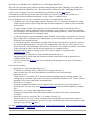
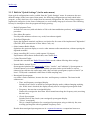
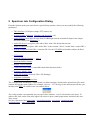
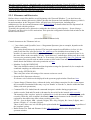
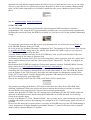
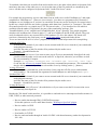
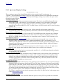
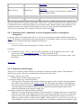
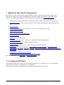
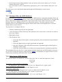
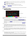
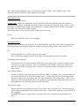
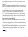
Frequency control panel (in SpecLab's main window)
(frequency control tab)
Controls on the 'Freq'-tab in the main window:
VFO (Variable Frequency Ocillator "tune frequency")
Tuning frequency for the 'VFO' in an external SDR, like SDR-IQ, Perseus, or an external hardware
controlled via Audio-I/O- or ExtIO-DLL. In configurations without 'controllable' frequency
conversion, leave this field zero. Note: In additon to the 'VFO frequency', there is another frequency
offset which may be added to the display - see Radio Frequency Offset .
fc (center frequency for the spectrum/spectrogram)
Can be used to set the displayed center frequency manually. But in most cases, it's easier to move
the main frequency scale with the mouse.
sp (frequency span for the spectrum/spectrogram)
Can be used to change the displayed frequency range. But in most cases, it's easier to do this with
the zoom buttons, or with the content menu of the main frequency scale.
--- or, alternatively, instead of 'fc' and 'sp' : --f1 (minimum frequency for the spectrum/spectrogram display)
This an alternative to define the displayed frequency by 'fc' and 'sp' (center frequency and span).
f2 (maximum frequency for the spectrum/spectrogram display)
Together with 'f1', this is an alternative method to define the displayed frequency range.
Select between 'fc'/'sp' and 'f1'/'f2' with the options menu mentioned below.
opt ('options' button on the 'Freq' panel)
Opens a small menu with VFO / frequency related options:
Frequency controls: Center frequency and span, or min- and max frequency
Allows to switch between the two alternative style to define the displayed frequency range.
See explanation of the input fields 'fc'/'sp' and 'f1'/'f2' above.
Include VFO frequency on frequency scale
When checked, the 'VFO frequency' is included in the labels on the main frequency scale.
When not checked, the main frequency scale shows the 'baseband' (or 'audio') frequency
range.
Fixed display span at 1 pixel per FFT frequency bin
When checked, the 'frequency span' (sp) is automatically set to that each horizontal pixel
position on the spectrum/spectrogram exactly matches one FFT frequency bin.
Disable auto-apply and increment/decrement for frequency input fields
When checked, the 'frequency' input fields (VFO, display center, and display span) behave as
in older versions, without automatically 'finishing' the input, and without the possibility to
increase/decrease the current values via cursor keys or mousewheel. Input to those input fields
must then be finished manually with the ENTER key.
Spectrum Lab Manual
18 / 113
Values in the above 'frequency' fields can be entered directly (through the keyboard). In addition, you can
increment/decrement the current value with the cursor keys, or the mousewheel. The cursor position (not
to be confused with the mouse pointer) defines the stepwidth.
When typing a frequency into any of these three edit fields, you can enter expressions like "135.8k"
instead of 135800 if you like. The input will be converted to the standard notation when pressing ENTER,
unless the the 'auto-apply' option is disabled in the 'opt' menu mentioned above.
Other tabs of this control panel are explained in the next chapter, and -possibly- in other documents
because there may be more tabs than in the screenshot shown above.
See also: help index
back to top
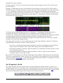
3.3.2 Time Axis
The "Time Axis" panel shows the current time and the time of the latest waterfall line. It may also be used
for scrolling the waterfall "back in time".
If the spectrum line buffer is large enough (larger than the number of waterfall lines on screen), you may
scroll the time axis of the waterfall "back to the past". Old parts of the waterfall which have already
disappeared from the screen can be made visible again, you may also zoom the old parts of the waterfall
using the controls on the "Frequency Axis"-panel or change their color using the controls on the "Color
Palette"-panel.
Shifting the slider on the "Time Axis"-panel to the RIGHT will scroll the contents of the waterfall back to
the past. The waterfall will stop it's real-time-scrolling as long as the time-slider is not in the leftmost
position. The FFT output will be recorded in the background then (but data collecting will not stop).
This situation is indicated by the "Time Axis"-panel changing its color from the usual gray to a light cyan.
As long as you see the "Time Axis"-panel in an unusual color, you know that the waterfall display is not
in "real-time"-mode but shows old data.
The amount of time (seconds, minutes, hours, or even days) is dictated by the waterfall scroll rate in
conjunction with the spectrum buffer size. The spectrum buffer size can be modified on a special tab of
the configuration screen,
Shifting the time-slider back fully to the LEFT will return to "real-time"-mode.
The "Time Axis"-panel also shows the current time ("NOW:") and the time when the latest visible
waterfall line has been recorded ("VIEW:"). In "real-time"-mode of the waterfall there will only be a
maximum difference of one FFT calculation interval between the "NOW"- and "VIEW"- time.
Note that the "Time Axis" panel (like all other time-indicators in this program) use UTC (=GMT) to be
independent of the earth's timezones. If you don't see the correct time shown in UTC on this panel, you
should check the time settings of your PC (double-click the time display in the task bar).
An alternative to the slider on the time-panel is the buffer-overview bar on the bottom of the main
window.
back to top
Spectrum Lab Manual
19 / 113
3.3.3 Cursor Position Display
The Cursor Position panel shows information about the current mouse (cursor) location.
The display on the cursor-panel depends on the cursor display mode, which can be switched by clicking
on the frame of the cursor panel. Some of the cursor display modes and -options are:
• Simple (one or two independent cursors)
• Delta (show frequency- and amplitude differences between the two cursors)
• Peak-detecting within narrow frequency range (the range is +/- 4 pixels along the frequency scale)
• Amplitude from mouse-cursor, not from plotted data (only works in the spectrum graph, not in the
spectrogram).
If this option is selected, the displayed amplitude is not related to the measurement, but only to the
cursor position.
• Let cursor #1 follow the mouse position
With this option, you don't have to click anywhere to change the position of readout-cursor #1
(red).
• Show info text near mouse pointer (shows frequency and amplitude of the mouse pointer position
as text near the pointer)
In "simple" cursor mode, the cursor display panel shows...
• The upper line in the cursor box usually shows the frequency for the mouse-position, or (if the
readout-cursor is fixed to a certain position), the frequency of the cursor's fixed position. In peakdetecting mode, the frequency may vary even if the pixel-position of the cursor (in the
spectrogram) is constant (like in fixed-cursor mode). The peak-detecting range is a few pixels on
the waterfall screen. The peak itself can be seen as a small green circle in the spectrum graph.
Note: the displayed frequency has a larger resolution, and usually also a larger accuracy than
dictated by the FFT bin width, thanks to a special interpolation subroutine.
• The second line usually shows the frequency (in Hertz) and the amplitude (decibel or percent)
related to the mouse position.
In Radio-Direction-Finder mode, the cursor box also displays the direction towards the transmitter
of the displayed signal (note that this RDF is frequency-sensitive).
• The third line may show other infos, for example the timestamp when the waterfall line under the
cursor has been recorded (hr:min:sec).
If the control bar on the left side of the main window is switched off, the cursor text is displayed on the
right edge of the main menu, so the cursor data can be seen even without the cursor display panel.
Note: Since May 2004, the text on the cursor panel can be selected with the mouse, and copied into the
clipboard (with CTRL-C as usual). This makes it easier, for example, to transfer the peak-frequency into
any other edit field, calibration table, or any text document.
For some special applications, you can retrieve the frequency , amplitude, and timestamp of the readout
cursor with the interpreter function spa.cursor.xxx .
Spectrum Lab Manual
20 / 113
3.3.3.1 Fixing the cursor on a certain frequency
The displayed data in the cursor window can optionally be fixed to a certain frequency, no matter where
you move the mouse. To achieve this, click into the spectrogram near the "frequency of interest" with the
right mouse button. In the popup menu which opens, select one of the "Set Cursor To..." functions.
To switch back from fixed-cursor to mouse-cursor mode, select the function "unlock cursor" in the
waterfall popup menu.
back to top
3.3.4 Color Palette Control
The Color Palette panel on the main window shows all colors that are currently used for the waterfall
display (a kind of "color legend").
The two sliders on the "Color Palette" control panel affect the brightness (B) and contrast (C) of the
waterfall colour assignment. This is an important feature if you are digging for weak signals, because it
allows you to enhance the readability on the fly ! The palette looks a bit different if the waterfall runs in
Radio Direction Finder mode, but the B & C controls work in both modes (in RDF/CDF mode,
Contrast/Brightness only affect the luminosity but not the color hue values).
Note:
If the brighness slider is labelled "b" (instead of "B"), the automatic brightness control ("visual
AGC") is active.
Double-clicking into the color bar starts the color palette editor.
At the lower side of the color control panel is a scale which usually shows some decibel values. Doubleclicking into the decibel scale switches to a certain part of the settings dialog where you can modify the
visible decibel range.
Note: Instead of cranking up the "contrast" slider to the maximum (to dig weak signals out of the noise),
you can also reduce the 'Displayed Amplitude Range' in the spectrum display configuration as explained
here . For example, if the "interesting" signals are all in the range -60 dB to -50 dB, don't use an
amplitude display range of -120 dB to 0 dB (instead, use -70 dB to -40 dB ).
See also: palette editor , visual AGC , help index
back to top
3.3.5 Progress Indicator/Stop Button
This button on the left side of the main window (under the contrast / brightness slilders) has different
functions, which will be shown as a text on this button.
The button's surface may...
Spectrum Lab Manual
21 / 113
• Show the current size of a log file (if file logging is active) and stops file logging
• Show the current position in the analyzed input file (if file analysis is active) and stops file
analysis
• Show error messages like shortage of buffer memory or too slow CPUs (during "normal"
operation)
• Show a hint as long as there are not enough samples collected for full spectral resolution
(i.e. "waiting for more data until the first FFT can be calculated" or "showing a preliminary, zeropadded FFT ")
Clicking on the progress button can take you to a more detailed error description, or clear (acknowledge)
a certain message .
back to top
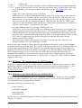
3.3.6 Programmable buttons
On the left side of the main window, there are a few programmable buttons (which you can only see if the
window is large enough..). These buttons are completely user programmable, both the text in the button,
and the function which will be executed when the user clicks one of these buttons.
To execute the button's programmed function, click it with the left mouse key or press enter when it's
selected.
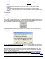
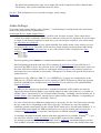
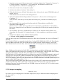
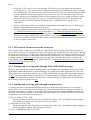
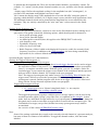
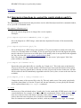
To change the button's programmed function and its text, click it with the right mouse key to open the
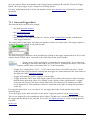
following dialog:
The field "variable String Expression for button text" defines the text on the button's face (caption). This
can be a simple fixed text string (embedded in double quotes), or a combined string expression like this:
"Time: "+str("hh:mm:ss.s",now)
More about this can be found in the description of Spectrum Lab's built-in interpreter, look for "string
expressions" there. If the button text is not a fixed string but a variable expression, set the checkmark
"evaluate and update caption periodically".
The field "Interpreter Command(s) to be executed on click with left button defines what shall happen
when the user clicks a programmable button. This is usually a sequence of interpreter commands
(explained in another document), but it is also possible to run external programs this way using the "exec"
Spectrum Lab Manual
22 / 113
command.
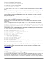
In the screenshot above, the 'capture' command is used to produce a screenshot which contains the current
date+time in the filename whenever the user clicks on the self-defined button "Capture now". However,
you can do an awful lot of other things with the programmable buttons once you know how to use
Spectrum Lab's built-in command interpreter.
The field "Hotkey" allows you to define a hotkey for the programmable button. Pressing the hotkey will
have the same effect as clicking on the button with the left mouse key (see above). An empty hotkey, or
the value zero means the button can only be activated with the mouse, but not through the keyboard. The
keyboard-combination must be entered as a decimal value (windows "virtual key" code, see below). The
code can be easily found by clearing the hotkey field, and pressing the hotkey (on the keyboard, for
example F1). If the hotkey edit field is empty, it will automatically be filled with the decimal value. A few
decimal keyboard codes are shown below.
F-Key
F1
F2
F3
F4
F5
F6
F7
F8
F9
F10
F11
F12
code (without
SHIFT etc)
112
113
114
115
116
117
118
119
120
121
122
123
with SHIFT key
(= code + 256)
368
369
370
371
372
373
374
375
376
377
378
379
with CTRL key (=
624
code + 512)
625
626
627
628
629
630
631
632
633
634
635
Usually the programmable buttons are used to invoke interpreter commands (as explained above). But
those buttons on the left side of the main window can also be controlled through SL's command
interpreter. Here is an example to change the background colour of the first (i.e. topmost) button:
button[1].color = 0xC0FFFF : REM change background to light Cyan
The format of the hexadecimal colour codes is similar to HTML: 0xRRGGBB, where each of the three
components (RR=red, GG=green, BB=blue) ranges from 00 = minimum to FF = maximum brightness.
0x000000 is black, 0xFF0000 is pure red, 0x00FF00 is pure blue, 0x0000FF is pure green, 0xFFFFFF is
bright white. A negative colour value restores the button's dull grayish background colour.
If the button number is omitted, the interpreter will access the button which is currently been 'executed'
(eg. clicked). This way, a button can change its own colour when clicked, or when its hotkey is pressed.
See also: String expressions, command- and function overview, Index .
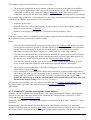
3.4 Controls on the bottom of the main window
To open an additional control bar on the bottom of the main window, select "View/Windows"..."Control
bar on bottom" in the main menu. Some of the controls in the bottom bar are explained below (but not all,
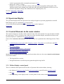
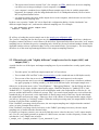
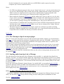
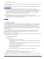
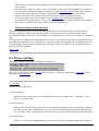
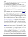
because this is still "in the making"). If this control bar is visible, the bottom of the main window may
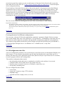
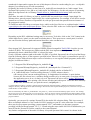
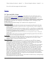
look like this:
The screenshot also shows a part of the main spectrogram. The bottom control bar below it contains an
overview of the spectrum buffer (which can be configured through a menu). It only makes sense to turn
this control bar on if the spectrum buffer covers a larger timespan than the main spectrogram. If you don't
need this control bar, turn it off using the popup menu in the lower right corner.
Spectrum Lab Manual
23 / 113
3.4.1 The Spectrum Buffer Overwiew (in the bottom control bar)
The narrow spectrogram in the control bar contains an overview of the buffer contents. By default, the
whole buffer is visible, but you can also zoom in with the buttons on the right side. The part of the buffer
which is visible in the main spectrogram is marked with a small red or green rectangle. Red colour means
"the main spectrogram is scrolled back in time", green colour means "the main spectrogram shows the
most recent data, it is NOT scrolled back".
To scroll back and forth, you can grab the indicator rectangle with the mouse and move it left or right.
Because the overview may be zoomed, you can alternatively use the navigation buttons which are
explained below.
3.4.2 Navigation buttons to scroll through the spectrogram buffer
The two buttons next to the overwiev can be used to scroll the main spectrogram through the buffer, pageby-page (the left button jumps further into the past, the right button from past to present, until the
indicator turns green as explained above).
The two zoom-buttons can be used to zoom the buffer overwiew (they do NOT affect the main
spectrogram !). This is helpful if the buffer contains a really HUGE amount of spectrum lines, for
example an overnight recording.
The menu button in the bottom control bar opens a small popup window where you can find some options
for the spectrogram overview, one of them is to open the configuration screen with the spectrum buffer
settings.
Last modified: 2011-09-15 (YYYY-MM-DD)
Spectrum Lab Manual
24 / 113
4 Spectrum Displays
Overview (about spectrum displays)
• Spectrum Graph
• Waterfall Display (classic spectrogram)
• Main Frequency Scale
• Radio Station Frequency List
• Reassigned Spectrogram
• 3D Spectrum Display
• Correlogram
• Single- or dual-channel operation of the spectrum analyser
• Spectrum averaging (overview)
• The "second spectrogram"
See also: Spectrum Lab's main index, display settings, Controls on the left side and on the bottom of the
main window (separate documents).
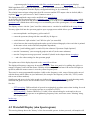
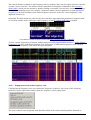
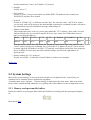
4.1 Spectrum Graph
This graph shows the spectrum as a line plot. One axis of this graph is the frequency domain (with an
optional display offset), the other is the amplitude (linear or logarithmic, depending on the current FFT
output type).
Spectrum Lab Manual
25 / 113
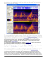
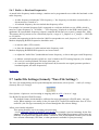
(spectrum graph, frequency scale with filter passband controls, and spectrogram display)
With logarithmic FFT output, the amplitude scale is in decibels (about 90 decibels maximum). The 0-dBpoint can be set anywhere from the display configuration dialog (or by command).
The relation between input voltage into the A/D-converter and the FFT output value in decibel (dB) is
explained here (use your browser's "back" button to return..)
The displayed amplitude range can be modified in the setup dialog.
As an overlay for the spectrum graph, a reference curve can be displayed, a peak-holding curve (which
shows the largest peaks from the previous XX seconds; green in the screenshot above), and an average
spectrum curve (which shows the average over a selectable part of the spectrogram; red in the screenshot
above).
The display colours -also the "pens" used for various curves- can also be modified in the setup dialog.
You may right-click into the spectrum graph to open a popup-menu which allows you to:
• turn an amplitude- and frequency grid on and off
• rotate the spectrum (along with the waterfall) by 90 degress.
• switch between "split window" and "full-size plot" (no waterfall)
• select between the normal graph mode and a special coloured-bargraph, where each bar is painted
in the same colour as the waterfall (amplitude-dependent).
• turn the "peak holding graph" on and off (in the submenu "Spectrum Graph Options")
• turn the "momentary" (non-averaged) graph on and off (in the same submenu)
• turn the "long term average spectrum" on and off (details in the chapter about averaging)
• ... and a few other settings for the spectrum graph
The update-rate of this display depends on the waterfall scroll rate.
The displayed frequency range may be modified with the Time Axis panel or by pulling the (yellow or
orange) frequency scale with the mouse. Hold the left button pressed and move the mouse left/right (or
up/down) while the mouse cursor is over the yellow frequency axis.
There may be some programmable markers visible on the frequency scale, some of them can be moved
with the mouse while others are just 'indicators' (for example: the frequency of the LO ("VFO") can be
tied to one of these markers).
Small green and green circles in the graph area indicate the data-readout-cursor in peak-detecting mode,
small red and green crosses are the readout-cursors in normal (non-peak-detecting) mode.
See also:
• FFT Averaging : Different kinds of spectral averaging help to reduce noise when looking for weak
but coherent signals. Averaging operates on a sequence of FFTs.
• FFT Smoothing : Further reduction of "visible" noise when looking for weak and incoherent
signals. Smoothing operates on neighbouring frequency bins, and causes some "blurring" along
the frequency axis.
back to top
4.2 Waterfall Display (aka Spectrogram)
This moving bitmap shows the "history" of the last recorded spectra. As time proceeds, old samples will
Spectrum Lab Manual
26 / 113
be scrolled out of view; but they can be scrolled back with the time slider on the "Time" panel (in the
upper left corner of the main window).
(stereo spectrogram with amplitude bar and log frequency scale)
The intensity (amplitude) of a particular frequency affects the color of a pixel in this bitmap. The relation
between amplitude and color can be controlled by a contrast- and brightness control panel on the left side
of the main window. Additionally, you can turn on the "visual AGC" function to let the program adjust the
brightness value automatically, when the noise level (in the displayed frequency range) changes.
In it's original form (with the "water" falling down), the X-coordinate of a pixel is derived from the
frequency-axis, and the Y-coordinate is the time axis (depending on the "scrolling speed" which is
adjustable under the display settings).
The visible frequency range can be modified by pulling the frequency scale with the mouse (hold left
mouse button down with the mouse pointer over the frequency scale).
The displayable frequency range and -resolution depends on the FFT settings (size, decimation, center
frequency) and the audio sample rate. For example, an FFT with 40 uHz resolution requires about 1 / 40
uHz = 2500 seconds, or about 7 hours, to collect the equivalent number of samples.
If the waterfall runs in RDF mode (radio direction finder), the colour of the waterfall shows the angle of
arrival, while the brightness shows the signal strength. More on that in this separate document.
For long-term observations of "narrow bands", the spectrogram screen can optionally be split into
multiple "strips", which will be vertically or horizontally stacked (depending on the orientation of the
frequency scale: if it runs vertically, small spectrogram strips will be stacked vertically, with the newest
strip on the top and the oldest on the bottom). The height of the strip is configured in the display settings.
Spectrum Lab Manual
27 / 113
The number of strips is only limited by the screen size. Notes:
• The multi-strip waterfall will not be redrawn completely if contrast or brightness are modified.
• For very special applications, a new strip can be started anytime (even if the previous line has not
reached the maximum with), using the command water.new_strip . This can be used, for
example, to synchronize the multi-strip display to full UTC hours (follow the link for an example).
Like in many other components of the program, you can activate a context-specific popup menu by rightclicking into the display. Some options for the waterfall are:
• Frequency grid overlay
• Waterfall Time Grid : Allows time markers as a grid overlay (over the spectrogram), and/or text
labels in various formats - read more.
• Rotation of the display by 90 degrees (=vertical or horizontal frequency scale)
• etc ...
If the main window shows a combination of the Spectrum Graph and the waterfall, both are separated by
the scrollable frequency scale (which applies to both).
Notes:
• Click into the waterfall with the left mouse button to show the spectrum graph for that line of the
spectrogram for about two seconds. It will look like the spectrum graph is frozen for a short time,
but this is done deliberately. To freeze the waterfall display for an unlimited time, use the
Start/Stop menu (stop "Spectrum Analyzer #1", which is the one in the main window).
• Click into the waterfall with the left mouse button, and hold the button pressed while moving the
mouse to mark a rectangular area. When releasing the button, a special popup menu appears. In
that popup, you can select special functions like the spectrum replay function.
• Click into the waterfall with the right mouse button to open a popup menu, which gives quick
access to some important parameters without having to open the display control panel.
• The waterfall colour palette can be selected by clicking into it. You can also define your own
colour palette as described here.
• Every calculated FFT spectrum will be drawn in the waterfall as a colored graphic line which is
one or two pixels high (or wide, depending on the orientation). So, if the "scroll rate" is set to 200
milliseconds, the waterfall will move down (or left) by 10 graphic pixels per second.. but:
If the CPU cannot keep up with the waterfall speed, the waterfall will scroll slower than you
defined in the display settings ! That's not a bug, it's a feature ;-)
The program can periodically save the contents of the waterfall. See periodic and scheduled actions.
Experienced users can control the waterfall display via interpreter commands (even from other
applications).
4.2.1 Visual AGC (for the spectrogram colour palette)
Normally, the colour palette of the spectrogram is only controlled through the contrast- and brightness
slider on the left side of the main window. But optionally, you can turn on the "visible AGC" on the
second tab of the Spectrum Display settings.
Technically, the term AGC = automatic gain control is a bit misleading. In fact, the "visual AGC" works
as follows:
When painting a new line into the waterfall, the program first measures the noise level within the
displayed frequency range, as explained here. Then, it subtracts this value (actual noise level in dB) from
the reference value, which can be set in the display settings window (typically -100 dB). Next, this
Spectrum Lab Manual
28 / 113
difference (deviation) is passed through a simple low pass filter, depending on the visual AGC speed
(slow/normal/fast). When painting the waterfall, the low-pass filtered deviation is added to all FFT bins,
before converting them into a colour values.
The "visual AGC" avoids that the spectrogram image will not get too dark or too bright if the input signal
level changes. This happens, for example, if the spectrogram shows a shortwave radio signal, and the path
loss changes dramatically, or (for some reason) the local noise level rises.
One of the downsides of the visual AGC is, you cannot tell the signal strength (voltage, power, or
whatever) from the colour in the spectrogram display. You may be fooled by the AGC, when a narrowband signal "disappears", which in fact is just overwhelmed by broadband noise. Without the AGC, you
would have seen that the noise went up. So be sure to turn on this AGC only if you really need to.
Note:
As a reminder that the visual AGC is enabled, the brightness slider is labelled "b" (lower case) when
the AGC is on. To turn it off, click on the "b" to change it back to "B" ("B"=AGC turned off,
brighness only controlled through the brightness slider).
4.2.2 Amplitude Bar (alongside the spectrogram display)
An optional amplitude bar can be displayed on the side of the waterfall. It can show the "peak" value of
the input signal in the time domain. Unlike the waterfall display, the amplitude bar is not limited to a
certain frequency range. It often looks like a seismogram (and in fact, has been used as such already):
The background of the amplitude bar is blue. The amplitude from the first input
channel adds green colour, the amplitude from the second channel adds red
colour (if the analyser is configured for dual channel mode, of course). So if the
bars from both channels overlap, the result is white.
Other data can be plotted in the amplitude bar, too. For example, the red curve
in the screenshot above shows the current noise level. Their pen colour, content,
and scaling range are all defined in the "watch window" (where they can also be
plotted in a separate window). Do define which of the watch-window's data
channnels shall be plotted into the amplitude bar, open the display configuration
screen.
back to top
4.3 3D Spectrum Display
The 3D spectrum adds another dimension (the time) to the display, but is often less easy to read than the
waterfall display.
Spectrum Lab Manual
29 / 113
To switch the main display window to "3D Spectrum", open the spectrum display dialog (from the main
menu: "Options".."Display Settings"), then select "3D Spectrum" in the combo list labelled "Show".
It is important to select a "strong" colour palette, with as many colour transitions as possible, and to adjust
the displayed amplitude range carefully. Without a suitable colour palette, you will hardly see anything on
the 3D spectrum. The colour palette is controlled the same way as for the spectrogram.
Furthermore, it helps to turn on the option "Amplitude Grid" in the display settings for a better readability
of the amplitudes. But still, in the authors opinion, a 3D spectrum display is not particularly suited to read
the amplitudes accurately. But it can help to see the amplitudes (y axis) versus frequency (x axis) and time
(z axis, here: pointing from the foreground into the background).
Special options (which only apply to the 3D spectrum) are on an extra tab in the configuration window.
Besides that, the following options also affect the 3D spectrum display:
• the background colour: defined on the "Display Colours" panel, labelled "Spectrum Graph
Background"
• the colour used for drawing the scales around the graph: on the same panel, labelled "Spectrum
Graph Grid"
• the option "Mirror for Lower Side Band" (on the 2nd tab of the display settings), which reverses
the frequency scale
• the "Displayed Amplitude Range" (usually in dB), can be modified in the configuration window
too
back to top
4.4 Reassigned Spectrogram
Under certain conditions, reassigned spectrograms provide more resolution along the frequcency- and the
time-axis than the classic spectrogram shown above. For comparison, a zoomed conventional
spectrogram (1st) and a time/frequency reassigned spectrogram (2nd) with the same FFT parameters :
Spectrum Lab Manual
30 / 113
More about reassigned spectrograms in a separate document; a few configurations with reassigned
spectrograms can be recalled from the Quick Settings menu.
back to top
4.5 Correlogram
The correlogram is a rarely used function. It is a special graphic representation of the 'similarity' of two
signals, or the 'randomness' in a signal.
More specific, it can be used as a cross-correlation plot (if the two inputs of the analyser are connected to
different signal sources), or an auto-correlation plot (if both inputs are connected to the same source. The
correlator itself doesn't care about that).
The graphic shows a plot of the correlations r(h) versus h (the time lags). In Spectrum Lab, the
correlogram uses the same fourier-transformed sample blocks used for the "normal" spectrogram. In fact,
the correlogram runs side-by-side with the main spectrum display (spectrum graph and/or spectrogram, as
Spectrum Lab Manual
31 / 113
explained in an earlier chapter).
For that reason, the range of time lags delivered by the correlator depends on the FFT size of the main
spectrum display.
Example: A soundcard delivering 11025 samples/second, feeding a 65536 point FFT, will fill a buffer
with 65536 points (in the time domain) in 5.94 seconds. The maximum displayable time lag range will be
+/- 2.97 seconds then, with lag zero in the middle. The following screenshot shows the spectra and
correlogram of a strong noise signal with weak sine wave added. A 0.5 second delay line (using SL's test
circuit) was added between the signal generator and channel #1 of the analyser. Channel #2 was directly
fed with the test signal (no delay).
To activate this correlation display, select 'View / Windows' .. 'Correlogram' from the main menu. A
correlation test (like the one described above) is contained in the SL configurations folder,
"CorrTest1.usr". If the spectrum analyser is only connected to one input channel, the correlogram (and the
correlation graph) will show the autocorrelation (correlation of the input signal with itself).
The displayed lag range can be modified by pulling the scale with the mouse (the same way as with the
frequency scale in the other display modes).
The output of the correlator is *not* normalized to the average input amplitude. Instead, the following
scaling and sign convention was chosen (quite arbitrarily):
• A sine wave, with the maximum possible amplitude (just below the clipping point) fed into both
analyser inputs, will produce 100 % output at the time lag where both signals coincide.
• If the signal at channel #1 leads the signal at channel #2, the maximum correlation will be at some
positive lag (don't ask why..)
• If the signal at channel #2 leads the signal at channel #1 (aka Ch1 lags Ch2), the maximum
correlation will be at some negative lag
Due to the FFT windowing, the coefficients at the edges of the window (extreme lags) may be attenuated.
This may be compensated in a future version of SL, if required for some application (it can be avoided by
using a rectangular FFT window ). At the moment (January 2009), the correlator / correlogram is so rarely
used that putting more effort in it doesn't seem justified.
4.6 Frequency Scale
The visible frequency scale is located between spectrum graph and waterfall (if both are visible). It is
usually horizontal ("X-axis") and shows only a part of the processed audio spectrum (which is defined by
the FFT settings). You can add or subtract a user-defined offset if you want. You can also split the scale to
zoom into two independent ranges. The frequency scale may look like this:
Spectrum Lab Manual
32 / 113
The colored rhombic symbols on the frequency scale are markers (they may be simple indicators but also
versatile control elements). The markers can be controlled via interpreter commands in the frequency
marker table, which you can activate by double-clicking on a marker. You can move a marker by holding
the left mouse button pressed. For example, a frequency marker can be connected to a signal generator's
frequency, to the local oscillator of the audio frequency converter, to the AFC center frequency of the
digimode decoder, etc.
Optionally, the main frequency scale can also show the three most important parameters (frequency shift
as 'zero beat' marker, lower, and upper edge frequency) of the FFT-based audio filter. Example:
(screenshot of main frequency scale with filter passband display / controls)
To show certain 'frequencies of interest' without using one of the programmable markers, a 'Radio Station'
Frequency List can be loaded into Spectrum Lab. Frequencies of radio stations appear as thin coloured
lines in the main frequency scale and in the spectrum graph.
(VLF spectrum/spectrogram with 'Radio Station' display)
4.6.1.1 Popup menu of the main frequency scale
Clicking into the frequency scale (on a particular 'frequency of interest', not on one of the frequency
markers) with the right mouse button, opens the frequency scale's popup menu:
The menu contains some frequently used functions. Most of the entries should speak for themselves,
Spectrum Lab Manual
33 / 113
some are explained in the next chapters.
4.6.1.2 Adjusting the visible part of the frequency scale
The displayed frequency range can be modified by pulling the visible frequency scale with the mouse
(left button pressed). Or right-click into the interesting part of the frequency scale and select "Zoom In" or
"Zoom Out" in the popup menu.
Alternatively you can enter the "edge frequencies" (Min + Max) in the frequency control panel on the left
side of the main window:
(frequency scale control panel)
More information about the frequency control panel is here.
Splitting the frequency scale into two ranges
Can be activated from the display settings dialog or from a popup menu which opens when you click the
frequency scale with the right mouse button. Use it, for example, if you want to have an "audio band
overwiew" on the left side of the screen and a zoomed display of a certain frequency range on the right
side. The separator between both scale sections can be moved with the mouse (not necessarily in the
center of the screen !).
Note:
If the option "split frequency scale" is set, but only one input channel active for the spectrum
analyser, both sections show different frequency ranges of the same signal. If two input channels
are active for the spectrum analyser (showing different signals on one screen), the frequency scale
will be split into two sections automatically.
To modify the frequency range of a frequency scale section, first click into the section on the visible
frequency scale. The frequency scale control panel will then show "Freq1" or "Freq2" instead of "Freq",
and the edit fields will apply to one section only.
4.6.1.3 Adding or subtracting a user-defineable frequency offset (for the display)
On the frequency control panel, you can enter a frequency offset which will be added to the displayed
frequency. This does not affect the internal processing, it is just for the "optics".
If you want to SUBTRACT the displayed frequency from a certain value (for example because you have
an LSB receiver tuned to 138kHz), enter the value "-138k" in this field. After three seconds, the entered
value will become effective (the entered value will be normalized), and the frequency scale will be
updated with the new settings. (Note: for LSB receivers, you should additionally activate the "LSB
mirror" in the settings menu).
back to top
4.7 One or two channels for the spectrum display
No matter if your soundcard has one or two input channels, the main frequency analyser can be switched
to "two-channel" mode. Both channels can be tapped to different points in the test circuit, for example
Spectrum Lab Manual
34 / 113
channel #1 can be connected to the left audio input, and channel #2 to the right audio input. Or, channel
#1 may be connected to the "input signal" (before the DSP chain) and #2 to the "output signal" (which
goes to the D/A converter).
The channel selection can be modified in the circuit/component window, which can be opened from the
"View/Windows" menu.
If two input channels are active for the spectrum analyser (showing two different signals on one screen),
the frequency scale will be split into two sections automatically.
back to top
4.8 Spectrum Averaging (Overview)
For some special "weak signal" applications, Spectrum Lab offers different ways and stages of averaging.
Averaging can be superior to simply increasing the FFT size, if the observed signal is "broad" (incoherent;
phase-, frequency- or amplitude modulated, etc).
There are various stages of (spectrum-) averaging, which will be explained in some depth later:
• "Internal average" at the FFT-calculating stage: This is a simple averaging of powers (or energies),
directly after the FFT calculation, using a leaky integrator.
This kind of averaging is always possible, even if the waterfall scrolls faster than the time required
to collect new data (in the time domain) for a single FFT. It is configured on the "FFT" panel in
the "internal average" field. This kind of averaging can help to see weak signals in the waterfall
display, for the expense of "smearing" along the time axis.
• "Waterfall line average": If the waterfall scroll interval is longer than the time to aquire data for a
"new" FFT, a larger number of FFTs will be calculated and added, before a new line is added to
the waterfall display (and shown in the spectrum graph). This kind of averaging is active when the
scroll interval (t_scroll) matches the following criterion, and the option "optimum waterfall
average" is selected in the Display Settings:
t_scroll > (FFT_size / sampling rate) .
The number of FFTs added this way (into a single "spectrum", which will then be displayed in the
graph and/or waterfall) depends on the waterfall scrolling speed, the audio sampling rate, and the
FFT size. The interpreter function water.avrg_max returns the number of FFTs added in each
line of the waterfall (you can use this function to calculate the "gain" from this incoherent
averaging, as explained somewhere below).
Unlike the first average option ("internal average"), this kind of averaging does not cause a
"smeared" display, for the expense of a slowly scrolling waterfall.
• "Triggered average": This special kind of averaging only works when the waterfall screen runs in
"triggered, non-scrolling" mode. It can only be used for periodic signals, for example in the "low
power moon radar" experiment, where a large number of VHF pulses were sent to the moon, and
the reflections collected over a long time before they became visible on the spectrogram (which
was synchronized with the transmit/receive interval).
To configure this kind of averaging, open the 3rd(?) tab of the Spectrum Display options (with the
panel "Options for Triggered Spectrogram"). Set the checkmark for "triggered spectrum", and set
the trigger control to "one SWEEP of the spectrogram" (=one waterfall screen).
Details about this special kind of averaging can be found in the "Alpha" VLF beacon example .
• "Long term average (spectrum)" : This option was added for the Earth-Venus-Earth experiment at
the IUZ Bochum in 2007. The long-term average is basically a second stage of averaging (after the
"FFT internal average" and the "Waterfall line average". Later (in 2011), an optional exponential
decay was added for the long-term average. The long-term average can be enabled on the first part
Spectrum Lab Manual
35 / 113
of the Spectrum Display Settings. The long-term average spectrum display works as follows:
All spectra (FFTs) which are displayed on the waterfall are added to the so-called long-term
average (with some optional preprocessing, as described in the document about the Earth-VenusEarth experiment).
The long-term average spectrum is displayed only as an additional curve in the Spectrum Graph
window (not in the waterfall !). This is typically a red curve, but the colour may be modified
through menu 'Options'..'Spectrum Display Settings' (part 3). When active, the long-term average
is painted with the fifth pen ("Pen 5", which is RED by default), as defined on the 'Display
Colours' panel.
The total number of FFTs added in the long-term spectrum average can be calculated with this
formula (to show it on one of the programmable buttons, as used in the Earth-Venus-Earth
configuration):
spa.lta_cnt*water.avrg_max + water.avrg_cnt ,
where :
spa.lta_cnt = total number of waterfall lines(!) added in the long-term average spectrum,
water.avrg_max = number of FFTs added in each line of the waterfall ("waterfall line average"),
water.avrg_cnt = number of FFT added in the current (still invisible) waterfall line .
The long-term average can be cleared through the popup menu of the spectrum graph: Right-click
into the graph, then (in the popup menu) select "Spectrum Graph Options" ... "Clear long-term
average". In the same popup menu, the curves for the long-term average and the "momentary"
spectrum can be turned on and off.
Alternatively, the long-term average can be cleared with the command "spa.clear_avrg". In the
EVE-configurations, one of the programmable buttons is used for this purpose.
Since 2008-03, the long-term-average spectrum can also be exported as a textfile, controlled by
the interpreter .
Since 2011-11, an optional 'exponential decay' can be configured for the long-term average. The
decay rate is specified as the half-life interval (auf Deutsch: Halbwertszeit), measured in minutes,
on the first panel of the Spectrum Display settings, close to the checkmark which enables the longterm average spectrum in the main spectrum display. Note that the 'counter' of spectra added into
the long-term average buffer is also affected by the exponential decay, thus even the 'counter'
value (spa.lta_cnt) may be a fractional (non-integer) value, which is unusual for a "counter" - but
that's the way it is. If the half-life interval is nonzero, the 'counter' will asymptotically approach an
upper boundary value, which depends on the waterfall scroll rate (i.e. the interval at which new
FFTs are calculated), and the half-life time.
• "FFT Smoothing" : Doesn't calculate an average from consecutive FFTs, but on neighbouring
frequency bins within a single FFT. Together with the other averaging options mentioned above,
this may help to reduce the 'visible' noise in the spectrum display if you are looking for very weak
signals. Details about FFT(-bin)-smoothing are here .
4.8.1 The "Second Spectrogram"
This is a simple "second" spectrum analyser, not as versatile as the display in the main window. You can
use it to display another portion of the spectrum, or analyze another audio source if you have a stereo
soundcard (or 2-channel ADC).
To open a window the second spectrogram, enter the "View/Windows" menu of the main window, then
select "Second Spectrogram". To activate the spectrum analyser for the second window, and select the
source, use the "Mode" menu of the second spectrogram window.
Notes:
• You can also activate the second spectrogram from SpecLab's circuit/component window, where
you can also see where the input for this analyser comes from. Click on the small "source" label to
Spectrum Lab Manual
36 / 113
open a list of all available sources.
• Some interpreter functions like "peak_a" and "peak_f" can operate on the spectrum from the
second spectrum analyser also.
back to top
Last modified: 2013-12-09: Added width and size info in the embedded images,
so they will be correctly sized when converting the help system info PDF (doc/SpecLab_Manual.pdf) .
Spectrum Lab Manual
37 / 113
5 Spectrum Lab Configuration Dialog
From the Options menu you can activate a special Setup window, where you may modify the following
parameters:
• TRX Interface (COM port settings, PTT control, etc)
• System Settings (timezone, filenames and directories, etc)
• Audio Settings (don't miss the note about feedthrough from the soundcard's input to the output,
and some oddity with Windows 7 !)
• Audio File Server (to replace ADC and/or DAC with a file-based data stream)
• Audio I/O DLLs (to replace ADC and/or DAC with a custom "driver", loaded from a simple DLL)
• Winrad-compatible ExtIO DLLs; Interface DLL for the FiFi-SDR (and similar software defined
radios)
• FFT Settings
• Spectrum Display Settings , ... part 2
• Spectrum Buffer Settings
• Display Colour Settings
• Colour Direction Finder (a waterfall-based radio direction finder)
• Frequency Marker Table
• Audio File Settings (formerly 'Wave File Settings')
• Amplitude Calibration
• Settings and Configuration files
The 'Configuration and Display Control' panel is a tabbed window, which can be opened from SL's main
window through the main window. For example, Options ... FFT Settings in the main menu will take you
directly to the 'FFT' tab visible in the screenshow below.
The config window can optionally stay on top of other windows, even if it doesn't have the focus. To
achieve this, click on the icon in the upper left corner to open a small popup menu, and check the item
'Stay on top'.
See also: Spectrum Lab's main index , user-defined menus , test circuit , installation hints ,
troubleshooting , some applications .
Spectrum Lab Manual
38 / 113
5.1.1 Transceiver Interface Settings
This item in the Setup dialog is used to define the COM port number where a "RX/TX" (=PTT) line and
other control signals can be connected.
• PTT Control:
The hardware required to use this feature is exactly the same as for many PSK31-programs. For
example, the RTS line of the serial interface can be set HIGH during transmit and LOW during
receive. The signal actually used can be selected on this control panel. There are some interpreter
commands to access this port, too. Alternatively (if there's no free COM port), consider using a
pilot tone for PTT control.
• CW Keying:
Will be used to generate a slow CW keying signal.
• Alert Bell:
This output can be driven by the Spectrum Alert function. A low signal means "no alert" (bell off),
a high signal means "ALERT !" (bell should ring, warning light flashing etc).
• use SmallPort driver to access I/O ports
(removed, because either direct I/O port access or the "smallport" utility caused severe problems
under Win XP, and most likely under any later version of windows)
• PTT pilot tone (frequency)
Can be used for PTT switching through a weak pilot tone generated by the soundcard. This is an
alternative to control a transmitter if your PC doesn't have a free COM port for this purpose.
Whenever the transmitter shall be ON ("sending"), a pilot tone with the specified frequency is
added to the output audio signal for the soundcard (approx. 20 dB below the max. output level,
added to the signal at label "L5" in the circuit). Use a simple PLL tone decoder like the LM567 or
similar to detect the pilot tone, and convert it into a switching signal. Note: The LM567 is marked
as 'obsolete part' but it's still easy to find, cheap, and easy to use.
To disable the PTT pilot tone, set the frequency to zero (the default state). Beware to place the
pilot tone outside of the transmitter's frequency range, but keep it below the half sampling rate:
For example, use 5000 Hz is about the maximum if the soundcard runs at 11025 samples/second.
The group "Radio Control Port" can be used if Spectrum Lab shall be used to remotely control a suitable
receiver (a "real radio"). Details can be found in the chapter "Interpreter commands for Remote Control".
The parameters are:
• Serial port number
Note: At the moment, don't use the same port as for the PTT control (set the PTT control port to
"none" if your PC only has one serial port)
• Bits/second
Some old ICOM radios used 1200 bit/second, others use 9600 bit/second. Check your radio's
manual !
• Data bits
Set this parameter to "8" which works for 99% of all cases ;-)
• Parity
Spectrum Lab Manual
39 / 113
Set this parameter to "none" for ICOM's CI-V protocol
• Stopbits
Usually set to "1"
• Flow control
Set this to "none", because most radios use neither RTS/CTS (hardware flow control) nor
XON/XOFF (software flow control)
• Protocol
Set this to "ICOM CI-V", or different (one fine day). The selection "none / ASCII-Text" means
you can only send ASCII strings to the radio through an interpreter command, but there will not be
any manufacturer-specific translation, message acknowledge etc.
• Address of the Radio
This hexadecimal value (with "0x" prefix) must match the "CI-V Address" of the radio. You will
find the default value in your radio's manual. Here are some values for ICOM radios (more at
http://www.plicht.de/ekki/civ ) :
Model
IC-735 IC-751A IC-725 IC-706 IC-706MkII IC-706MkII-G IC-756 ...
Address
0x04
0x1C
0x28
0x48
0x4E
0x58
0x50
...
Note that for the "older" three HF radios, the frequency is sent with 8 digits only, while for all
"newer" radios 10 digits are exchanged. So if you set the CI-V address of your IC-706 to 0x04 in
its menu, SpecLab will think it's an old IC-735 and only send 8 digits (which fails if the frequency
above 99 MHz). So better keep the radio's default settings, and select the right address in
Spectrum Lab.
• Master Address (for CI-V protocol)
Usually set to 0xE0... at least this is what ICOM uses in their own examples.
back to top
5.2 System Settings
Most of the 'system settings' are not saved in the normal user configuration file - instead, they are
considered to be 'machine' but not 'application' dependent.
To modify them, select 'Options' ... 'System Settings' in Spectrum Lab's main menu. Most items listed
below can be reached through submenus, or by picking one of the tabsheets on the configuration screen.
5.2.1 Memory and spectrum file buffers
Define the number of spectrogram lines buffered in RAM (for scrolling back the spectrogram display),
etc.
More details here.
Spectrum Lab Manual
40 / 113
5.2.2 Audio Server Settings
Explained in another chapter .
5.2.2.1 Timezone
Difference between local time MINUS UTC(GMT).
A few examples:
• enter "2" if you are in Germany, BeNeLux, France, and windoze has adjusted your PC's clock for
daylight saving time (MESZ)
• enter "1" if you are in Germany, ... , and windoze has adjusted your PC's clock for winter time
(MEZ)
• enter "0" if you are in Great Britain, Portugal, etc; it's winter time or if you have convinced
windoze not to fool around with your PC's clock in October
• enter "-5" if you are on the east coast of Canada or the USA (EST).
Alternatively, Spectrum Lab can ask the operating system for your timezone. If the 'timezone' information
on your PC, including daylight saving time, is configured correctly, set the checkmark labelled
[ ] get time zone information from system .
With this setting, you don't need to care about the offset between UTC and your 'local' time (with or
without daylight saving).
5.2.2.2 Geographic Location
Enter your own location here, using the Maidenhead locator system, or by latitude / longitude lin degrees,
minutes, and seconds .
This information will used in some exported files (for example, in wave files) if no GPS receiver is
available. Used for radio direction finding.
5.2.3 Timer Calibration
In this edit field, the precise frequency of a CPU-internal timer can be defined. This timer is used as a
"high-resolution" timebase. Its frequeny is often 3.58 MHz, in some PCs only 1.79 MHz. The nominal
value is queried automatically, but for some special applications you can enter the precise frequency here.
5.2.4 Clock Source for timestamps:
Defines the clock source for timestamps (in spectra, waterfall time grid, and the "time"-function which is
used in export data definitions). These options are avaliable:
• Use audio sampling clock only: Gives the best resolution and almost no 'jitter' because the time is
calculated from the count of audio samples, plus an "offset" to get date+time. If you use a
'calibrated' sampling rate, or even an external A/D converter, this option is the best choice.
• Slowly pull towards PC's real-time clock: Provides a better long-term accuracy in some cases,
especially if the audio sampling rate is drifting or not calibrated. With this option, the timestamps
are always very close to the PC's real-time clock (usually one second or less).
(temporarily removed:)
Daily clock error :
The daily drift of your PC's "real time clock". Unit is seconds per day. Use the DCF77-decoder, a radiocontrolled clock or the evening news on TV to find this value. Use this feature only if you really need it,
Spectrum Lab Manual
41 / 113
and only if your PC runs in a thermally stable environment for a long time. If your PC's RTC is too slow,
the value must be negative. The Reset button clears the number of accumulated 'compensation' seconds.
Use this button after correcting the PC's clock from an external program. Internally, the program keeps a
copy of the time when the clock error was zero.
5.2.5 Filenames and Directories
Defines where certain files shall be saved. Beginning with Vista and Windows 7, you don't have the
freedom to chose arbitrary directories (folders) because the Spectrum Lab installation directory, which is
located somewhere in the 'Programs' folder, will only have read permission, including all its
subdirectories. See the external document called 'Data Folders' for details about how the Spectrum Lab
installer will deal with this problem.
To modify the currently active directories (within the data folders), select Options .. System Settings ..
Filenames and Directories in SL's main menu. This opens the configuration window and switches to the
tabsheet shown below.
(screenshot of the 'Filenames' tab)
Control elements on the 'Filenames' tab are:
• [ ] use relative path if possible, base: c:\Programme\Spectrum (just an example, depends on the
windows version).
This option should always be checked. The base path cannot be modified here, in fact, it is the
path for all 'data files' specified in data_file_paths.txt (a file which has been written by the
installer). It cannot be modified by Spectrum Lab under certain windows variants because it's in
the same folder as the executable, aka the "install directory", and all these folders only have readbut not write-permission under Vista & Co. If necessary, you can modifiy data_file_paths.txt with
a text editor, but you will need an admin account (at least under Vista and Windows 7). More
details about data folders with write permission are here .
• Machine Config: MCONFIG.INI
This is the default location for all machine-dependent settings for Spectum Lab, for example the
soundcard sampling rate calibration table.
• User Config: SETTINGS.INI
This is the place where all settings of the current session are saved.
• Spectrum Ref (Spectrum reference):
A reference curve which can be displayed in the spectrum graph window. Details are here.
• Capture Image: Filename (base, without the index, and without extension) for the screen capture
aka screenshot. Destination folder may vary, but "thanks" to Vista & Co, must be within the data
folder (with write permission).
• Command File: File loaded into the command interpreter window during program start.
• Audio recorder: Path and file mask (with nnnn for the serial) for the internal audio recorder.
The meaning of the 'template' option is explained here (in the document about the triggered audio
recorder). Basically, it the 'template' checkmark is set, certain characters in the filename will be
replaced by date and/or time later (when recording starts), like:
YYYY = year (4 digits), MM = month (2 digits), DD = day (2 digits), hh = hour (2 digits), mm =
minute (2 digits), ss = seconds (2 digits).
Three or more lower case 'n's will always be replaced with the file sequence number (regardless of
the 'template' option).
• Radio Station List: Path and filename for the radio station list which can be displayed in the
spectrum window.
Spectrum Lab Manual
42 / 113
By default, the installer places only a few sample files in the 'frequencies' folder within the data
file directory. They can be modified with a text editor.
See also: TRX (transmitter/receiver) interface settings, audio settings,
back to top
Audio Settings
To open the audio settings dialog, select "Options"..."Audio Settings" from Spectrum Lab's main menu.
Some of the parameters are explained here:
Audio Input Device, Audio Output Device:
Select which audio device ("soundcard") shall be used for input or output. These combo boxes
contain all available soundcards, ASIO drivers, and more exotic devices which may be used as input
or output for the digitized samples. In most cases, you will use these controls if your system really
has more than one soundcard.
The audio device selection boxes may appear disabled if the audio stream comes from (or goes to)
an external audio server. The audio server may be a simple interface program which reads analog
samples from an external A/D converter, or one of the Audio I/O DLLs (explained in a later
chapter).
Entries beginning with a number are standard multimedia drivers (not ASIO).
Entries beginning with an A: (but not a device number) are ASIO drivers. If an ASIO driver is
selected as the INPUT device, the selection for the OUTPUT device is disabled, because in this case
the same ASIO driver will be used for in- and output. ASIO provides a lower latency between inand output, but is not available on all systems. Clicking the 'Ctrl' button will open the ASIO driver's
channel selector.
Input devices like "SDR-IQ / SDR-14" (-2) or PERSEUS (-3) require an extra hardware on the
USB port, or a TCP/IP connection to a server running a USB/TCP-IP gateway. More info on using
SpecLab with SDR-IQ is available in an extra document. If you want to use SL with PERSEUS,
read this document .
In addition to the input devices listed above (standard soundcards, ASIO, and the two natively
supported Software Defined Radios), you can add support for other 'special devices', if you have a
suitable "driver" (interface DLL) for it. Details about selecting / "installing" such an interface are in
another chapter. After installation, such drivers are either listed by their filename, or (depending on
the type) by a short name after a prefix D: ("Driver").
For some of these devices, additional settings may be necessary. Use the 'Ctrl' button after selecting
the type of the device. Depending on the device type, the 'Ctrl' button may open the standard
soundcard volume control panel (for the selected WAVE audio device, but not under Windows 7), or
a special SDR control panel (for SDR-IQ and Perseus), or a special control panel to select & or
configure an audio I/O DLL, or open the control panel of a Winrad-compatible ExtIO-DLL.
To exchange uncompressed audio streams with other applications (for example, Winamp(tm) ), you
can select also select the Audio-I/O-library (a special DLL) instead of the soundcard.
For absolute measurements, the input amplitudes must be calibrated. Amplitude display units like
Volts or dBuV only make sense if the relationship between A/D converter value and absolute input
Spectrum Lab Manual
43 / 113
voltage is known. Otherwise, stick to the default amplitude display unit which is "dBfs" (dB relative
to full scale) .
Other sources, other destinations :
These links take you to another tab of the configuration dialog, where alternative sources and
destinations for digitized audio (or quadrature IF streams) can be configured. This includes audio
servers and -clients, which can be connected through different ways (UDP/IP, TCP/IP,
WM_COPYDATA messages, periodically written audio files, etc). The WM_COPYDATA method
was, for example, used to receive data from the "winamp-to-SpecLab" plugin, which is described
here.
If the "local" soundcard is used for in- and possibly output, you don't need to care about these other
sources and destinations.
Sampling Rate:
The nominal audio sample rate of the soundcard, which is the number of samples per second read
from the analog/digital converter.
Both sound-input and -output use the same sampling rate (dictated by hardware). You should use
the lowest possible sample rate allowed by Shannon's theorem: With 8000 samples per second, you
can process signals up to 4000 Hz. Don't use higher sample rates just because your soundcard
supports them ! Only for very special applications (like the "VLF radio"), sample rates up to 192
kHz may be necessary. SpecLab works with sampling rates up to 192kHz, but only a few cards
really support such high sampling rates. Caution, the windows multimedia driver will happily
deliver any sampling rate - even if the hardware doesn't support it (it will be interpolated then,
which is not really helpful).
Some cards can play dirty tricks when you use 48000 samples per second (because they don't
support 48000 sampling), which leads to "phantom signals" on the waterfall. See the notes in the
"VLF Radio" application.
Some other cards play dirty tricks when running in full duplex (which means input + output running
at the same time): For example, the input- and the output sampling rate may be slightly different.
More details in the chapter about output resampling. (use a different output sample rate; any ratio
between 0.5 and 2.0 is possible).
Other stupid soundcards don't support 44100 Hz (which is surprising because that's the Audio CD
standard).
If you are running Windows 7 (and most likely any later windows version), and want to use the
soundcard at 48 kSamples/second and more, don't miss this note (defeat anti-aliasing through the
windows system control).
Also don't miss the sampling rate calibration if you use the program for the first time, or have
installed a new soundcard.
If a soundcard really supports a certain sampling rate (like 48000 Hz / x or 44100 Hz /x) is not
always easy to tell, because if the sampling rate 'requested' by the application is not really supported
by the hardware, the driver software (or the windows multimedia system) jumps in, and tries to
interpolate / extrapolate to realize the sampling rate by software. Unfortunately, Windows does a
really bad job on some machines. For example, on one of the author's PCs (a Lenovo Z61m), when
trying to run the onboard audio device at 12000 samples/second, the signal sounded 'distorted', and
the CPU load caused by the 'SYSTEM' process (indicated in the Windows Task manager) went up
to 5 Percent, as long as the audio input was running. Switching back to 11025 samples/second cured
this problem, the audio sounded 'clean' again, and the CPU load caused by the 'SYSTEM' process
went back to zero.
Again, it's not easy to tell which sampling rates are really supported, so if you find strange effects /
poor audio quality / dropouts / unexplainably high CPU load, try a different sampling rate - first try
a fraction or multiple of 48000 Hz (like 12000, 16000, 32000, 480000, 96000). If that doesn't work
well enough, try a fraction or multiple of 44100 Hz (like 11024, 22050, or 44100), especially on
'old' machines because sampling rates of 44100/N were the standard in the age of Soundblaster and
Co.
Spectrum Lab Manual
44 / 113
Last not least, it's possible to compensate the sample rate drift continuously, for example for phase
measurements or high-accurary frequency measurements.
Sampling Rate Divisor:
Defines the decimation ratio between the analog/digital conversion rate and the processing rate of
all following stages (which you can see in the component window, for example frequency
converter, digital filter, but also the Spectrum Analyzer).
Reducing the sample rate at this early stage is especially helpful if you run out of CPU power,
because -depending on what you are doing- the real-time sound processing threadwhats_a_thread
can 'eat up' a lot of the available CPU time. The internal processing rate is:
<Sampling Rate> divided by <Sample Rate Divisor>, for example:
11025 samples per second, divisor set to "2" will give an internal processing rate of 5512.5 samples
per second. This would be enough to process audio signals below 2kHz (theoretically 2756 Hz, but
this is impossible because of the anti-alias-filter's roll-off).
Note: After this decimation stage, and before the FFT calculation, there may be more decimation
stages. See 'FFT Settings'.
Bits per sample
Defines the resolution of the A/D converter. Usually 16 bits per sample. A few cards also support 24
bits per sample, resulting in more dynamic range (only required in rare cases though). Has only
been tested -with positive result- with the Soundblaster Audigy 2 ZS, but the difference between 16
and 24 bit per sample can only bee seen if the input signal is *very* weak. With most 'real-world
signals' you won't see a difference in the spectrum, unless you have the ultimately pure sine wave
generator on your workbench. The theoretic dynamic range with 24 bits is somewhere near
20*log(2^24) = 144 dB, more realistic are 108 dB as specified for the Audigy 2 card.
For most applications, stick to a resolution of 16 bits per sample.
Use anti-alias filter
has no effect at the moment, because the anti-alias filter is always enabled if the Input Sample Rate
Divisor is set to 2 or higher.
The anti-alias filter's length may be adjustable in future releases.
I/Q input adjustment
Switches to a submenu of the circuit window, where the gain balance and phase errors from an
image-cancelling direct conversion receiver can be compensated. More details can be found in a
separate document (if you don't know what a direct conversion receiver is, you don't need it
anyway.. )
Sample Rate Calibration Table
Because the true sample rates used by some soundcards (also expensive ones!) differs significantly
from the 'nominal' value, you can enter the true values for a number of standard 'nominal' rates in
this table. The "one-time" sampling rate calibration procedure is explained in another file. For
normal audio applications, you don't need this.
In rare cases (depending on the soundcard), the conversion rate of the ADC and the DAC can be
different. Since Version 2.7, Spectrum Lab contains a resampling function which can cope with this
problem, but it requires some additional CPU power (see the notes about soundcards with slightly
different sampling rates in the next chapter).
If you are looking for extreme frequency accuracy, it is possible to continuously 'detect' or 'calibrate'
the sample rate but you need a stable reference signal).
Some soundcard oscillator drift tests can be found here .
Note: Besides these settings, be prepared to spend a few hours playing with your soundcard's own
"volume control panel" (or whatever the manufacturer called it), until you managed that the audio input
(from the "line-in" jack) only(!!) goes into the A/D converter, and the card's audio output (the "line-out"
jack) is only fed from the D/A converter, without annoying bypass. Read more about this in the document
about SL's installation. Since May 2004 there is an extra chapter for the Audigy 2 ZS (and possibly
similar cards by Creative Labs), because it was sooo complicated to achieve - but it can be done !
Spectrum Lab Manual
45 / 113
Trouble with Windows 7 / missing 'Wave Out Mix' in the recording source selection
In the soundcard Mixer Control of Windows 7, input controls like "Master record" and "Wave Mix " seem
to be missing. It seems to be impossible to select "what you hear" for input.
If you also miss these important 'mixer controls' under Windows 7, here's where to find them (thanks
Chris for answering the question in the Spectrum Lab User's group !) :
> If the 'Wave Out Mix' is hidden and not made obvious at all, try this:
1. Select sound from the control panel.
2. Select the recording tab.
3. Right click on the background of the tab and choose "show disabled devices."
4. Right click on Wave Out Mix and click enable.
5. Now it should work the same way as Wave Out Mix in Windows XP, allowing you to record any
sound your computer makes.
back to top
5.2.6 Adding a special driver for other audio input devices
Certain interface DLLs (Dynamic Link Libraries) can be added to the list of input devices (see previous
chapter). Click the "..."-button next to the input device combo (with soundcards, ASIO devices, certain
SDRs, etc).
The principle to "install" such a "driver" (actually, just select the driver's interface DLL for input) is
described here. The same method is used for Audio-I/O-DLLs and for Winrad-compatible ExtIO-DLLs.
Note: No other kind of DLL (besides ExtIO and Audio-I/O-compatible DLLs) can be "installed" this way.
After installation, such drivers are either listed with their complete path and filename (typically beginning
with drive name C:/) , or -depending on the type- with a short name after a prefix D: ("Driver DLL").
Note that file paths never have a space after the drive name, which distinguishes them from ASIO drivers
(prefix "A: " - note the space after the colon) and the short name of a Driver DLL (prefix "D: ").
The 'Audio I/O Libraries' (see next chapter) are just ONE example of such a 'special driver'. There may be
other, hardware-specific drivers (or at least interface-DLLs to the real driver) which can be installed in a
similar fashion.
5.2.7 The Audio I/O Libraries
( 2011-08-14: This function has been re-written, the new DLL is incompatible with older audio-I/O libs !
Older libs didn't support timestamped streams.
Details are in the Manual for the Audio I/O libraries (PDF available on-line, not contained in the spectrum
lab installer. )
To exchange uncompressed audio streams with other applications, you can select select the Audio-I/Olibrary (which is a special DLL) instead of the soundcard. For 'normal' applications which only use a
Spectrum Lab Manual
46 / 113
soundcard for input and/or output, the rest of this chapter will not be worth reading for you... so skip this
chapter if you intend to use SL with a soundcard.
Originally, the Audio I/O library (in the form of in_Audio.dll) was intended as an "audio output" from
Spectrum Lab's point of view, and as an "audio input" for Winamp(tm), for the sole purpose of streaming
audio from Spectrum Lab via Winamp. Details about in_AudioIO.dll and winamp at the end of this
chapter.
Since then, the audio I/O library (at least in_AudioIO.dll) has turned from a simple 'input plugin' for
Winamp into a general-purpose 'audio bridge' for various applications. For example, it can also be used to
connect two (or more) instances of Spectrum Lab, with pre-processed data passed from one instance of
the program to another.
To 'install' an audio I/O library as an input device, add it to the list of devices as explained under 'Adding
a special driver for other audio input devices'. Then, select the DLL as the new 'Audio Input Device' on
the Audio Settings tab as in the example below:
Depending on the DLL, additional settings may be necessary. To do this, click on the "Ctrl"-button in the
'Audio Input Device' panel (see the small screenshot above). This opens a new control panel, in which
you can select the directory paths and stream identifiers (more on that later):
Since August 2012, Spectrum Lab supports I2PHD's Winrad-compatible 'ExtIO'-DLLs besides its own
Audio-I/O-DLLs. The concepts are similar, and the DLL-host implemented in Spectrum Lab will
automatically detect which kind of DLL is selected for input.
If only a filename without a path to the audio-I/O-DLL is specified, Spectrum Lab will try load the library
from the following places, in the sequence specified below. However it's highly recommended to specify a
full path, because with each new major version of windows, we are urged to install programs (and/or their
plugins) in different folders !
1. C:\Program Files\Winamp\Plugins\in_AudioIO.dll (*)
2. C:\Programe\Winamp\Plugins\in_AudioIO.dll (default path for a 'German PC')
3. C:\Programmi\Winamp\Plugins\in_AudioIO.dll (default path for an 'Italian PC')
4. in_AudioIO.dll in the "current working directory" (CWD) ,whatever that is...
(the concept of the 'current working directory', as implemented in windows, is quite broken
because the file selector box (a windows dialog) modifies it by its own gusto, even when told by
the application not to do so, so don't rely on it. Spectrum Lab tries to set to set the CWD back to
where it should be after opening a file selector, but this isn't bullet-proof. Select the DLL manually
in this case, and make sure you pick the correct, and full path ! )
(*) If the Audio I/O Library is used as a gateway between Spectrum Lab and winamp, it MUST be loaded from winamp's
"Plugins" directory. Most applications (like streaming to the internet) don't require Winamp anymore; and in that case you can
install the DLL in other folders.
Don't be confused by the name "in_AudioIO.dll" - the prefix "in_" must be seen from Winamp's point of view : For winamp,
it's an input plugin. For Spectrum Lab, it's an output device, but it can also be used as a link between an audio-producer and an
audio-consumer. Thus "in_AudioIO.dll" can be used either as an audio input, or an output, but not both at the same time in one
program instance.
Optionally, you can specify a unique 'Stream ID' in the Audio-I/O-selection dialog. This is necessary if
there are multiple instances of the 'Audio-I/O-DLL' running on your PC at the same time. For example,
there may be one program providing a stream named "VLF", and another (or the same) program
providing a different stream named "VLF_2". If both using the same Audio-I/O DLL for distribution, you
must fill out the 'Stream ID' field to connect to the wanted channel.
Any further configuration of the audio I/O library is beyond Spectrum Lab's control. As shown in the
Spectrum Lab Manual
47 / 113
screenshot of the 'Audio I/O-DLL Selection for Spectrum Lab' above, there is a button with the 'hand
pointing right' :
It usually opens a special configuration screen in the DLL (if the DLL
supports it). The sample DLL ("in_AudioIO.dll") which is contained in SpectrumLab's installer will show
something like this:
Hint:
If an audio-IO-DLL is already selected as the 'input' in Spectrum Lab, you can open the DLL's
control panel through SL's main menu:
Options ... Show Control Panel for audio-input-DLL. The same applies to Audio-I/O and ExtIO.
There may be other 'Audio-I/O-DLLs' available - for example, DLLs used as drivers for 'exotic hardware'.
The above screenshot is just an example for such a DLL. Actually, "in_AudioIO.dll" can be used to
distribute a gapless, uncompressed audio stream from one source to multiple destinations ("readers"),
which are listed on the DLL's control panel. Winamp may be one of those destinations (from Winamp's
point of view, this DLL is an "input plugin"). The control panels of other I/O-DLLs may look completely
different, and it's unlikely that they will also operate as Winamp input plugins.
Again, details about the Audio-I/O-DLLs are available online (as PDF) in the Manual for the Audio I/O
libraries.
See also: Spectrum Lab Audio Settings, Sending audio from SpecLab to Winamp ,
Details about Audio I/O DLLs (web link), Overview (index) .
ExtIO-DLLs,
5.2.8 Using in_AudioIO.dll to stream audio into Winamp
Originally, the Audio I/O library (in the form of in_AudioIO.dll) was intended as an "audio output" from
Spectrum Lab's point of view, and as an "audio input" for Winamp(tm), for the sole purpose of streaming
audio from Spectrum Lab (acually a filtered VLF Natural Radio stream) via Winamp, and the Oddcast
plugin, to an internet audio server (Icecast). Details about that are beyond the scope of the Spectrum Lab
help system; you can find more info about using the Audio-I/O-library to connect Spectrum Lab to
Winamp here (external weblink, requires an internet connection, and describes the configuration of
Spectrum Lab, Winamp, Oddcast, and Icecast. Unfortunately, the development of Oddcast or "Edcast"
seems to have stopped.... see http://www.oddsock.org/ ).
For audio streaming applications, consider using Ogg/Vorbis instead of in_AudioIO.dll . Support for
outbound Ogg/Vorbis audio streams is integrated in Spectrum Lab; MP3 is not .
5.2.9 Using in_AudioIO.dll to stream audio from the first instance of Spectrum Lab
to other instances
For this application, it's not necessary to copy the in_AudioIO.dll into the winamp plugin folder, but
recommended. If you don't have winamp installed on your system, unpack in_AudioIO.dll into the
spectrum lab folder. This way, SL will find it automatically even if you didn't specify a full path.
The library 'in_AudioIO.dll' can be used to feed digitized audio from one writer (source) to multiple
readers (destinations). Example:
1. The first instance (of Spectrum Lab) reads samples from the soundcard, resamples them to the
precise nominal sampling rate (using the SR calibrator) and sends the processed samples to the
audio-I/O DLL. For this purpose, the configuration of the 1st instance has the 'Audio Input Device'
set to the soundcard (-1 = default wave input), and the 'Audio Output Device' is an 'Audio I/O
DLL' .
2. The second instance (of Spectrum Lab) has the 'Audio Input Device' set to the same 'Audio I/O
DLL' (same path, same file).
Spectrum Lab Manual
48 / 113
3. The third, and any other instance (of Spectrum Lab) have their 'Audio Input Devices' also set to
the same 'Audio I/O DLL' . Thus the same signal (produced by the 1st instance) can be processed
by multiple other instances of Spectrum Lab, without the need for a 'virtual audio cable' or
multiple soundcards connected to each other.
This is possible because the audio I/O libraries (at least "in_AudioIO.dll") support multiple
readers.
4. The same DLL (in the same folder) can also be loaded by other applications at the same time,
besides Spectrum Lab. This is possible because the DLL uses shared memory to distribute the
digitized audio stream. Details on how to use the audio I/O DLL in your own application are here
(external link).
See also: Spectrum Lab Audio Settings, Sending audio from SpecLab to Winamp , Winamp Plugins,
Details about Audio I/O DLLs (web link), Overview (index) .
5.2.10Using a Winrad-compatible ExtIO-DLL for input
(added 2012-08-19)
Since August 2012, Spectrum Lab supports I2PHD's Winrad-compatible 'ExtIO'-DLLs besides its own
Audio-I/O-DLLs. The concepts are similar, but the API is very incompatible. Fortunately the DLL-host
implemented in Spectrum Lab will automatically detect which kind of DLL is selected for input. You may
find an ExtIO-DLL for 'your' radio at winrad.org/. For SDR-IQ and Perseus, this is not required because
these two radios are supported natively by Spectrum Lab.
To 'install' an ExtIO-DLL ("driver") for input in Spectrum Lab, select "Options" .. "Audio Settings" in
SL's main menu.
Then, click on the three-dotted button to select a driver for the new input device:
Next, select the 'driver' (actually just an interface DLL). This may be an ExtIO-DLL (filename begins
with "ExtIO" and ends with ".DLL", which you only see if you reconfigured the STUPID windows
environment so it doesn't hide known extensions by default). Note that for some/many/all ExtIO-DLLs it
may be necessary to install them into the same directory where the application is installed (in this case,
SpecLab.exe). Reason: Some DLLs don't find certain auxiliary files when the 'current directory' is not the
same as 'their own' directory. This is stupid, but that's the way things are.
Here, for example, the ExtIO-DLL to control PERSEUS:
After that, Spectrum Lab prompts you for additional parameters which may be passed to the DLL on
initialisation. The ExtIO-DLLs don't support command line arguments, so in most cases you can leave the
'parameters' field empty:
Only if the ExtIO-DLL doesn't provide the digitized samples itself, but relies on the soundcard for input,
the name of that soundcard must be entered in the 'parameters' field shown above. In certain cases, SL can
make an 'educated guess' for the name of the soundcard. For example, the FiFi-SDR identifies itself as
'FiFiSDR Soundcard' to the windows multimedia system, thus after selecing 'ExtIO_Si570.dll' as the new
input device, Spectrum Lab will preset the 'parameters'-field with the string 'FiFiSDR Soundcard'; but it's
your decision to modify this box as necessary.
Spectrum Lab Manual
49 / 113
Spectrum Lab will add the complete path to the DLL in its list of "input devices" now, so you can easily
select it (or any other device) quickly by picking it from the list. There is also a button ("Hand pointing
right") on SL's audio input panel (see screenshot) which may take you to a hardware-specific control
panel.
See also: Audio Settings, Audio-I/O-Libraries .
5.2.10.1 FiFi SDR
The FiFi-SDR is a small software defined radio with an integrated USB soundcard. It contains a
programmable VFO, using the Si570 (programmable oscillator chip). As an (almost) fully assembled kit,
including the preselector board, the SDR was available for 130 Euros in 2012 at the german Funkamateur
Verlag:
To control this cigarette-box sized HF receiver from Spectrum Lab, you will need a special ExtIO by
Fred, PE0FKP, filename 'ExtIO_Si570.dll'.
Do a web search for 'SoftRock Ensemble Configuration Tool'. The installer for Fred's 'driver DLL' used to
be at pe0fko.nl/CFGSR/, along with a nice tutorial. Note that the FiFi-SDR is only one of a couple of
Si570-based radios supported by this DLL.
A similar ExtIO-compatible interface for the FiFi-SDR may work, too; but none (besides Fred's) was
completely tested by the author of Spectrum Lab.
An alternative DLL named 'ExtIO_FiFi' was found somewhere, which seemed to work for a while, but it
always crashed when trying to open the control panel (ExtIO: "ShowGUI"). The DLL was dumped for
that reason.
Details about the FiFi-SDR, developed by German radio amateurs (on their 'FichtenFieldDay', thus the
name) used to be at o28.sischa.net/fifisdr/trac and www.ov-lennestadt.de/.
Unfortunately, the FiFi-SDR hardware seems to be better than the control software. On the author's PC,
controlling the VFO frequency (through ExtIO_Si570.dll) often stalled. If 'your' FiFi-SDR also doesn't
react on changes in the VFO frequency, don't make the same mistake by changing the settings on the
ExtIO_Si570 control panel ! Instead, unplug and re-plug the USB connection. In most (if not all) cases,
the VFO worked properly again afterwards.
Here are the settings used for the FiFi-SDR, on the ExtIO_Si570 control panel:
The preselector settings on the ExtIO_Si570 don't seem to have any effect for the FiFi-SDR: After
soldering 8 additional LEDs to the preselector board to indicate the preselector switches, it became
obvious that the microcontroller drives the preselector switches automatically.
Another note about the FiFi-SDR: On a PC running trusty old Windows XP, the FiFi-SDR's soundcard
delivered 96 kSamples/second, and the observable bandwidth was 96 kHz (but with severe aliasing
effects at the extreme edges).
On a PC with Windows 7, 32 bit, "Home Premium", the very same device, same soundcard, only showed
a 48 kHz wide band even when the sampling rate (configured in SL's 'Audio Settings' panel) was also set
to 96000.
How to cure this annoyance is shown below; if you have an EASIER way to get the FiFi-SDR running at
a 'true' sampling rate of 96000 Samples/second under Windows 7, please let me know. Here's what the
author tried on a german Windows 7 machine:
Spectrum Lab Manual
50 / 113
1. Open the system control ("Systemsteuerung"), switch the display from "Kategorie" ('Category' ?)
to "Kleine Symbole" ('Small Icons' ?). On a german PC, this window was titled "Alle
Steuerungselemente", if that means anything to you.
2. Click on the 'Sound' icon (loudspeaker symbol) .
3. Switch to the tabsheet "Aufname" ('Recording' ?)
4. With a bit of luck, you will find a 'Microphone' there, followed by the name 'FiFiSDR Soundcard'
(stupid, isn't it ?).
Click on that device to select it for the changes below.
5. Click on the button labelled "Eigenschaften" ('Properties' ?). Do not click on "Konfigurieren"
('Configure' ?).
With even more luck than you already had, this button opens yet another well-hidden propery
panel.
6. On the german PC, the control panel had the stupid title "Eigenschaften von Mikrofon"
('Properties of Microphone' ?)
(Microsoft seems to think that every audio source connected to a soundcard's is a 'microphone',
but you can change the text from 'Mikrofon' to something like 'SDR', and pick another symbol for
the device)
7. On the tabsheet 'Erweitert', 'Standardformat', 'Wählen Sie die Abtastrate und die Bittiefe aus'...
(Something like 'Extended' (?), 'Standard format' (?), 'Select sampling rate and bits per sample'
(?) )
8. Switch from '2 Kanal, 16 Bit, 48000 Hz (DVD Qualität)
to '2 Kanal, 16 Bit, 96000 Hz (Studioqualität)' .
After the above steps, the FiFi-SDR showed the full 96 kHz wide in Spectrum Lab, also on a Windows 7
machine.
Fred's ExtIO_Si570.dll was manually installed into C:\afusoft\FiFi-SDR\ExtIO_Si570.dll . This full path
must be added to Spectrum Lab's list of audio devices (under 'Options'..'Audio Settings', click on the
three-dotted button to select the file). After that, SL's Audio I/O configuration tab should look like this:
Note: Unlike noted elsewhere, the ExtIO-DLL doesn't need to be copied into the Spectrum Lab folder.
With a full path specified as in the above screenshot, SL will load the DLL, and if the DLL itself is smart
enough, it will be able to load other files (if needed) from its own installation folder.
With the ExtIO_Si570 loaded, Spectrum Lab will look for a name like 'FiFiSDR Soundcard' in the list of
'audio devices' offered by the windows multimedia API. If that doesn't work (because on your PC the
'FiFiSDR Soundcard' has a different name), declare the FiFiSDR Soundcard as the 'default audio input
device' for windows. That way, if SL doesn't find a device which looks like a FiFiSDR (soundcard), it will
use the default WAVE input (device "-1").
This is necessary because unlike most other 'ExtIO'-DLLs, ExtIO_Si570 doesn't deliver the digitized I/Q
samples from the radio. ExtIO_Si570 only controls the radio's VFO (it doesn't even control the nice
bandpass filters aka "Preselector Board" in the FiFiSDR, at least not in ExtIO_Si570 V2.6 which was the
version used for these tests).
5.2.11 Output resampling
(added 2007-11-09)
In certain cases, the sampling rate of the audio output (DAC) may be different from the sampling rate of
the input (ADC).
Example:
Spectrum Lab Manual
51 / 113
• The input comes from an external "box" (for example, an SDR), which uses an exotic sampling
rate that is not an integer multiple of your computer's soundcard,
• your computer's soundcard uses slightly different sample rates for the in- and the output (this
happened, for example, with the integrated audio device in Thinkpad notebook). How to notice
this is explained further below.
• you want to connect an exotic audio output device to the computer, which doesn't use one of the
'standard' audio sampling rates
In these cases, open the "Audio I/O" tab in SpecLab's configuration dialog. Set the checkmark "use
different output sample rate", and enter the nominal sampling rate. For example:
[v] use different output sample rate:
nominal : 22050 Hz
SL will try to lookup the precise sample rate in the sample rate calibration table.
The "precise" sampling rate for the output may be a bit difficult to find out if you don't have a hardware
frequency counter, but there is a trick how to do this below. SpectrumLab needs to know this "real" output
sampling rate to calculate the precise resampling ratio, which may be any fractional number (thanks to an
algorithm similar to those explained at http://www-ccrma.stanford.edu/~jos/resample/ ). The next chapter
describes on of the most important applications of the output resampling function.
5.2.12Soundcards with "slightly different" sample rates for the input (ADC) and
output (DAC)
A quick check to see if the input- and output sampling rate of your soundcard are exactly equal (as they
should) :
• Turn the option "use different output sample rate" off (see above)
• Turn on both ADC and DAC in the circuit window (so the soundcard runs in full duplex mode)
• Turn on one of the sine waves in the test signal generator, and connect it to the output
• Let the generator run for several minutes, and listen to the tone. If you hear a clean note without
any gaps (popping or clicking sounds), you don't need different input- and output sample rates !
Otherwise, in the main menu, select "View/Windows"..."Debugging Window". On the Debug tab, there
are indicators for the input- and the output buffer usages. Watch the display for "OutBuf=XX %" and
"InBuff=XX %". Typically (if all works well in full duplex mode), the output buffer is filled to 40 .. 60
percent, and the input buffer is filled to 0 percent. Why ? As soon as input samples are received from the
soundcard, they are processed; so the input buffer is ideally empty most of the time. On the other hand,
the output buffer must not run empty - otherwise, there is the chance of interrupted audio output (which
you hear as "popping" or "clicking" sounds). When the audio processing starts, the output buffer is filled
to about 50 percent of the available space.
If the "OutBuff" percentage slowly decreases, the true output sampling rate is higher than the nominal
value (as in the example shown above).
If the "OutBuff" percentage slowly increases (or the "InBuf"-percentage increases), the true output
sampling rate is smaller than the nominal value.
If you have a frequency counter, you can easily find the correct value for the true ("real") output sample
rate: Use SL's test signal generator to produce a 1000 Hz tone, measure it with a frequency counter, and
calculate the "real" sample rate as below:
f_sample_real = f_sample_nominal * f_test_measured / f_test .
Spectrum Lab Manual
52 / 113
Example: f_sample_nominal = 22050 Hz, f_test = 1000 Hz, f_test_measured = 1006.8 Hz
-> f_sample_real = 22050 Hz * 1006.8 / 1000 = 22199.94 Hz .
After this, there should be no more input buffer overruns, or output buffer underruns... until you install
another soundcard !
back to top
5.2.13Multiple soundcards in one system
If you have more than one audio device (soundcards eg) in your system, you can select the audio input
and output which shall be used by Spectrum Lab in the audio settings.
Beware: The names which appear in the selection list are sometimes quite cryptic, like "Nr. 3 =
Hochwertiges Bluetooth-Audio" on the author's machine.
If there's only soundcard installed on the PC, leave both "Audio Input Device" and "Audio Output
Device" set to the default value (-1 = default WAVE input / output). The program will then use the first
available soundcard, which is usually correct.
Entries in the device selection lists which do not begin with a number are ASIO drivers. More information
on how to use ASIO is in this separate document .
See also: audio servers, audio I/O DLLs, ExtIO-DLLs, program start with command line parameters .
back to top
5.2.14Unexpected aliasing at 48 kSamples/second on a Windows 7 system
The following was suggested by a member of the Spectrum Lab user's group (- thanks Ed -) to eliminate
aliasing effects when trying to run the soundcard at 48000 samples/second or more under Windows 7 :
• Look into the sample-rate setting under the 'Advanced' setup in the properties of the sound
recording device.
(Control Panel > Sound > Recording tab, highlight your device and click Properties, then the
Advanced tab).
• You may find that W7 is setting your card up at the default 44.1, and everything else is resampled.
I see this with my Gigabyte onboard Realtek 889, W7 32-bit.
Tell W7 to use 48k and all will be well.
So, even though the audio hardware supported 48000 samples per second, and the application (Spectrum
Lab) requested 48000 samples per second from the "operating system", Windows 7 stupidly resampled
from 44100 to 48000 samples/second, causing signals above 22050 Hz to "fold back" at the Nyquist
frequency (= half sampling rate).
Most likely, the same also applies to higher sampling rates (96 or even 192 k, if the audio hardware
supports it).
back to top
5.3 Audio File Servers and Clients
It is possible to connect Spectrum Lab to an other application which serves as "remote Analog/Digital
converter" or "Digital/Analog coverter". The other application then acts as "Audio File Server" to replace
the audio input (ADC) and/or output (DAC). This may be used as an interface to any kind of exotic audio
hardware. (Note: You don't need this if SL shall analyze the audio input from your "local" soundcard !)
Spectrum Lab Manual
53 / 113
To establish a link between an audio client and an audio server, the audio client (which is Spectrum Lab)
must know the name of the audio server, or at least the name of the file produced or consumed by the
server. All this can be configured in Spectrum Lab's "Audio File Server" menu:
For example the program may receive audio data from an audio server called "SndInput.exe" and sends
sound data to "SndOutpt.exe". (These are just examples, I use these two programs myself. Instead of
SndInput.exe use SerInput.exe if you have an external A/D converter on the serial port. See notes below)
In this case, simple disk files are used to exchange audio data from "producer" to "consumer". The audio
file transfer protocol is very simple (not "FTP" for heaven's sake :-), it is described in a file which is
available from the author of Spectrum Lab (part of the sound utility package, files
"SoundUtilityInfo_01.txt" (english) and "SoundUtilityInfo_49.txt" (german). Two sample programs
which use the soundcard are written in plain "C", and are available on the DL4YHF website. They can
easily be adapted to drive any external A/D or D/A hardware. To drive the author's PIC-based A/D
converter (connected to the serial port), use the serial input utility mentioned further below.
To use an external A/D or D/A "server" program, fill out these fields in Spectrum Lab's setup dialog:
"consume ADC file"
Activate this checkmark if you want to use an external audio file server instead of your soundcard's
analog/digital converter,
and enter the name of the file which will be produced by the audio server.
Example: ..\SoundUtl\audio.dat
"to start A/D server"
This is an optional service if you want to start your A/D server automatically from SpecLab (only
possible when the audio server runs on the same PC as SpecLab, otherwise you will have to start
the server manually). Example:
Example: C:\SoundUtl\SndInput.exe /of=audio.dat /sr=11025 /ch=1 /dt=1
(Look into the A/D server's manual for the necessary command line parameters ! The command line
may be added automatically after you selected the server by clicking on the [...] button )
"to stop A/D server"
This is a similar command line as the one above, but to stop the A/D file server (and terminate
itself, usually..). The command line argument for both SndInput.exe and SerInput.exe is /quit .
"produce DAC file"
Activate this checkmark if you want to use an external audio file server instead of your soundcard's
analog/digital converter,
and enter the name of the file which will be produced by the audio server.
Example: ..\SoundUtl\to_dac.dat
"to start D/A server"
Works like "to start A/D server" (described above) if you want to start the D/A-conversion server
automatically from SpecLab.
Besides the "file-based" audio interface, it is possible to send and receive uncompressed audio streams via
UDP, TCP/IP, or other network protocols:
• Receive audio data through WM_COPYDATA messages
Select this option to receive audio data from the "Winamp-to-SpecLab"-plugin.
• Receive audio via UDP
• Receive audio via TCP/IP
• Send audio via TCP/IP
• Receive and send audio through an 'Audio I/O DLL' with shared memory (under development in
2011-08).
Spectrum Lab Manual
54 / 113
Notes:
• While the "A/D" server is in use, the message "File doesn't exist" may appear on the tabsheet
"A/D D/A Server". This is not an error. It only means that SpecLab looked for the audio exchange
file and didn't find it, because the server has not produced a new file since SL last deleted it. Under
normal conditions, the message toggles between "no error" and "file not found". If the "file not
found"-message never disappears, make sure the filenames are correct, and the A/D server writes
the file into the directory where SL expects it. It may be helpful to specify the full path for the
audio file, not just the pure filename (something like "c:\temp\audio.dat" instead of just
"audio.dat").
• SL uses 16-bit integer values (by default) to communicate with "audio file servers". This may be
different if decimated I/Q sample pairs are used.
• For more information about the "sound input" and "sound output" utilities, look into the file
?..\..\SoundUtl\SoundUtilityInfo_49.txt (in german) or ?..\..\SoundUtl\SoundUtilityInfo_01.txt
after downloading and unpacking the "sound/audio utilities" from DL4YHF's website. If you
already have a copy of DL4YHF's "Sound Utilities" on your harddisk: The SoundUtilityInfo-links
only work if you have downloaded these utilities and copied them into the same directory structure
as in my original "source files".
5.3.1 PIC-based A/D converter for the serial port
Since October 2002, a firmware is available for a PIC12F675 microcontroller which can be used as an
external A/D converter for 2 channels at exactly 2500 samples per second. Data are sent to the PC through
the serial port ("COM1" or "COM2"). PIC-Firmware and "interface driver" program ("SerInput.exe") can
be obtained from the author, or downloaded from DL4YHF's homepage. The "interface driver" program
is implemented as an audio server for Spectrum Lab (and almost any other application, written in any
programming language which can access simple disk files). See hardware desription for the PIC-based
serial A/D converter for more details.
5.3.2 Sending and receiving audio through WM_COPYDATA messages
Different audio-processing programs running on the same computer can send audio in real-time to other
applications without the need for an extra soundcard, or a virtual audio cable. Spectrum Lab (and a few
other applications written by its author) can use WM_COPYDATA messages. Details about the principle
are here. One application which uses this feature is an output-plugin for Winamp, which allows you to
play MP3 files (and audio streams received from the internet) directly into Spectrum Lab. Details about
the Winamp-to-SpecLab plugin are here.
5.3.3 Sending and receiving audio through a local network
For remote site survey, uncompressed audio can also be sent through a local network. For example, a
remote VLF receiver consisting of an old laptop PC with soundcard and WLAN adapter, located in an
electrically quiet place, can send an *uncompressed* audio stream for logging and further analysis into
the shack. The following controls (checkmarks and input fields) on the "A/D & D/A Server" tab on SL's
configuration screen are used for this purpose:
[ ] Receive audio via TCP / UDP
Set this checkmark, select the protocol, and define the (source-) IP + port number of the computer
from which you want to receive an audio stream (as a client).
[ ] Send audio via TCP / UDP
Set this checkmark, select the protocol, and define the (source-) IP + port number of the computer to
which you want to send an audio stream (as a client).
[ ] Act as a SERVER for audio-via-TCP/IP
Spectrum Lab Manual
55 / 113
Set this checkmark if your computer shall act as a SERVER for audio-requests from other
computers (the "clients" mentioned above).
Notes:
• For UDP (user datagram protocol), there are no "clients" and "servers", just one sender and at least
one receiver. When testing UDP on a shaky WLAN link, audible dropouts could be detected. But
UDP is such a nice simple protocol (it can easily be implemented on a microcontroller with
ethernet interface), that in some cases UDP may be better suited than TCP/IP.
• Don't confuse the integrated HTTP server with the audio-via-TCP-server, and never use the same
IP port number for these functions ! Though both use TCP/IP as the underlying protocol, they are
totally incompatible. If you try to connect the audio-via-TCP-server with a web browser, the best
you can expect is getting a message like "400 Bad Request - this is not an HTTP server !" .
• At the moment, no standard audio streaming protocol (such as RTSP) is implemented in Spectrum
Lab. But, there is the winamp-to-speclab plugin, so you can use winamp as the "bridge" between
SpecLab and such streams.
• The built-in protocol was designed to be simple, stupid, but as flexible as possible (including
timestamp, calibrated sampling rate, format descriptor, etc). A specification about the protocol use
in SpecLab will be available one fine day (if someone asks for it) .
back to top
5.3.4 The Winamp-to-SpecLab output plugin
Since it is rarely used, this plugin is not part of the Spectrum Lab installer. Instead, you can download it
from here - or, if the page has moved because I changed my ISP, search for "WINAMP -> Spectrum Lab
output plugin". That page also described the installation of the plugin (which means to unpack it, and
copying the DLL into Winamp's plugin folder).
It is an "output" plugin from Winamp's point of view. From Spectrum Lab's point of view, it is an audio
source like many others. SpecLab doesn't need to know that this particular plugin sends the audio data.
All you need to do within SpecLab is set the option Receive audio data through WM_COPYDATA
messages in one of the configuration tabs.
Some technical details about the communication between this (older) winamp plugin and Spectrum Lab
are explained here.
5.3.5 Sending audio from SpecLab to Winamp
The other direction (from Spectrum Lab to Winamp) is also possible, i.e. send audio from SpecLab to
Winamp. To do this, you will need another plugin (an "input plugin" from Winamp's point of view) which
can be found here (external link, not part of SL's online help system). If the link is broken, search the web
for "DL4YHF Audio I/O libraries". You will also find the sourcecodes, and a manual (PDF) for the audio
I/O libraries there.
In fact, the "SpecLab to Winamp" plugin (filename "in_AudioIO.dll") is a specialized audio-I/O-DLL
written for Spectrum Lab by its author. Note that unlike most other Audio-I/O-DLLs, it must be placed in
Winamp's plugin directory, and must not be copied anywhere else, to work properly. This restriction
doesn't apply to any other audio-I/O-DLL.
5.3.6 Loading Winamp plugins into SpecLab...
... turned into a nightmare, and was only possible with "ancient" plugins from Winamp Version 2.9 (and
older). The full story is here. It may still be working, but most of the plan was abandoned in 2008 .
See also: Audio-I/O-DLLs .
Spectrum Lab Manual
56 / 113
back to top
5.4 FFT settings
The FFT settings are on one tab of the Configuration and Display Control dialog. It can be opened from
the menu "Options ... FFT Settings". The following parameters can be adjusted :
Decimate FFT Input (formerly: Sample Rate Divisor)
An internal "sample rate divisor". This parameter is used to decimate the samples before the FFT
calculation. If the audio processing rate is 8000, and (for example) the "Rate Divisor" is set to 4, the
'internal' sample rate for the FFT input is only (8000/4=) 2000 samples per second, reducing the
CPU power and increasing the FFT resolution.
BUT: The higher the "Rate Divisor", the lower the maximum frequency that can be detected with
the FFT.
Note: The sample rate may have already been decimated at an earlier stage ! See 'Audio Settings'.
FFT input size
The number of samples that are processed by a single FFT calculation. Must be a power of 2. This
parameter influences the frequency resolution in the FFT output.
Since program version V1.2, the FFT Size does no longer define the speed of the scrolling
waterfall !
The higher you set the FFT size, the more frequency esolution you will get, but the longer it will
take to calculate an FFT. On slow PCs (<100MHz), you should leave the FFT input size below
16384 samples. If the CPU is too slow, the waterfall will scroll slower than it should !
A detailed discussion of FFT input size, decimation, sample rate and frequency resolution is here.
FFT window function
Selects the windowing function for the samples in the time domain. Each block of samples which
enters the FFT will be multiplied with this function, which usually has a shape of a raised sine
wave, with values near zero at the edges of the window, and one in the center. For most
applications, the Hann window (mistakingly called "Hanning") is often the best choice because it
has a good dynamic range (suppression of sidelobes) while maintaining a low equivalent noise
bandwidth. For details, search Wikipedia on "window function" (used to be on
en.wikipedia.org/wiki/Window_function). The window functions implemented in SL are:
Rectangle, Hamming, Hann, Gauss, Nuttall, Flat Top. They can also be set through the interpreter.
Notes on the FFT windowing functions:
- The equivalent noise bandwidth for the currently selected FFT parameters is displayed in the info
box below the FFT settings.
- The formulas of the FFT windowing functions are contained in the SL installation archive, in the
file 'Goodies/fft_windows.txt'. You can load that file with DL4YHF's "CalcEd" ("calculating
editor") to plot the windowing functions in a graphic window.
- for the experimental correlogram display, you may have to use the rectangular window .
FFT Type and Center Frequency
"Real-number FFT": Preferred type for all broadband applications, where the displayed frequency
range shall start at "DC" (0 Hz). No frequency conversion inside the spectrum analyser.
"Complex input with frequency shift": For narrow-band applications, if only a small frequency
range (centered around any audio frequency) is of interest. This only works together with a
decimation factor of 4 or higher. Internally, the analysed signal is multiplied with a complex
oscillator signal (the "center frequency"). The complex signal (with "I"- and "Q"-branch) is then
decimated, and the decimated signal (with a low sampling rate) is fed into a complex FFT.
"Complex input with separate I/Q channels": also a complex FFT, but no oscillator and complex
I/Q multiplier inside the frequency analyser. Instead, the I- and Q-branch is fed into the analyser via
two separate input channels. These two channels can be the LEFT and RIGHT input of a soundcard
running in stereo mode, or an external two-channel A/D converter. More information about I/Q
Spectrum Lab Manual
57 / 113
processing with Spectrum Lab is here.
Include F.O. calibrator (Frequeny Offset Calibrator)
This is only possible if the FFT type is set to "complex input with frequency shift". With this option,
the frequency error (measured by the frequency offset detector) is subtracted from the complex
oscillator frequency as explained in the previous paragraph.
Zero-pad input if not enough samples available yet
If this option (checkmark) is set, the FFT input will be padded with zeroes as long as not enough
samples are available for input yet.
This option can help to 'see something quickly' if the FFT size (length * decimator) is very large, as
in the 'very slow QRSS modes'.
FFT output unit
Select the display unit for the FFT results (for spectrum graph and waterfall):
V (volts), W (power in watt), and several logarithmic scales (dB, dBuV, etc).
The linear scales (voltage or power) are sometimes better to detect very weak signals in the
waterfall display, expecially with high noise floor.
The logarithmic scales ("dB" with different reference levels) are more common if the input signal
has a high dynamic range.
Absolute unites (like V, dBuV and a few others) only make sense after an amplitude 'calibration' as
explained here.
Hint: You can compare signal amplitudes directly in decibels with the "readout cursor" in the
spectrum display. The cursor function also uses the "FFT output unit" for display, so this name is a
bit misleading.
FFT internal average
This parameter may be important if you try to 'dig' very weak signals out of the noise.
A value of 0 will give no averaging, a value of 3 will already reduce the random noise a bit, and will
make the spectrum look smoother, so weak coherent signals crawl out of the noise on the
spectrogram display. The higher the average value, the greater the smoothing effect, but if the value
is too high the spectrum (and spectrogram) will react too sluggish. See also: Overwiev of different
averaging- and smoothing options.
FFT smoothing (parameter: number of neighbour bins)
This option can help to detect very weak, but relatively "broad" signals. The smoothing parameter
are the number of "neighbour" bins in the FFT which are averaged to form the smoothed spectrum.
Internally, a Gaussian kernel is used. Unlike FFT averaging (which operates on consecutive FFTs),
the smoothing option affects the shape of a signal (for example, it turns a 'sharp peak' from a
coherent signal into a wider (Gaussian) 'hump'. But if the signal is already a hump with a certain
bandwidth anyway, this option can help to squeeze the last fraction of a decibel out, so a signal
becomes visible in the spectrum display. Try to match the smoothed bandwidth to your observed
signal to get the best result with this function .. it may require some trial-and-error. The FFT
Smoothing was revived in SpecLab for the EVE experiment.
FFT output type
Set to "Normal (amplitude only)" for a normal spectrogram without phase (or radio-direction)
information,
or to "Complex (real + imaginary part)" for special applications - for example phase analysis,
or to "Radio Direction Finder" for a radio-direction-finding spectrogram where the colour indicates
the azimuth angle.
Note 1 : Some FFT output types don't affect the waterfall display, but only the FFT export (as file) !
Note 2 : The spectrum replay function (which transforms spectra back into audible signals) only
works if the FFT output is set to "complex", otherwise the phase information in the original signal
gets lost.
Note 3 : The triggered averaged spectrogram (with one average buffer for each of the spectrogram
lines) only works if the FFT output type is set to "Normal (amplitude only)".
Spectrum Lab Manual
58 / 113
back to top
5.4.1 Spectrum Display Settings
(last modified 2011-11-03)
These settings are part of the Setup Dialog which can be opened from SL's main menu via
"Options".."Spectrum Display Settings". Here just some parameters which need explanation. Parameters
with a (2) are located on the second part of the spectrum display settings (etc), because the space on the
first tab was not sufficient.
Vertical Frequency Axis
Affects the layout of the spectrum/spectrogram screen. The classic waterfall display scrolls from
TOP to BOTTOM, so the time axis is vertical and the frequency axis is horizontal. If the option
"Vertical Frequency Axis" is checked, the frequency axis will be rotated by 90 degrees and the
waterfall will scroll from RIGHT to LEFT (which is better for HELL modes and for visual decoding
of slow CW).
Logarithmic frequency scale (2)
With this checkmark set, the frequency scale for both waterfall and spectrum graph will be
logarithmically scaled (which is preferred by musicians). Otherwise the frequency scaling is linear.
Mirror for Lower Side Band (2)
Usually the lower frequency will be on the LEFT or LOWER side of the frequency axis. With this
option set ("checked"), the frequency axis will be mirrored so the lower frequency will be on the
RIGHT or UPPER side of the frequency axis (depending on the "Rotation" of the frequency axis).
Split frequency scale (2)
Allows to split the frequency scale for the waterfall and spectrum graph in two sections. The
frequency ranges of both settings can be defined independently. If the "split frequency axis" is
enabled, you can divide the screen area with the mouse on the small 'gap' between both parts on the
frequency scale. When the mouse cursor is replaced with the splitter symbol, hold the left button
pressed and move the mouse.
This option can also be activated from a popup menu on the frequency scale (use the right mouse
button to open a popup menu, while the mouse cursor is on a certain screen element).
Amplitude grid
activates a grid (overlay) for the spectrum graph, usually in 10- or 20-dB steps (depends on display
unit and height of the graph area).
Double-width waterfall lines
is an option added for high-resolution screens. With this option, each new line of the spectrogram is
drawn twice on the screen. If you have a monitor with a vertical resolution of 1536 pixels, try this
option if you cannot see individual lines in the spectrogram. The option is also good for fast nonscrolling spectrograms (waterfalls) without causing unnecessary CPU load (because it halves the
number of FFTs calculated per screen sweep).
One pixel per FFT bin
With this option enabled, the frequency scale will always be stretched so one screen pixel (along the
frequency scale) will represent exactly one FFT bin. The 'Max' frequency field on the control panel
on the left side of the main window will be disabled if this option is active (you can only enter both
'Min' and 'Max' frequency if the 'one pixel per bin' option is off). The benefit of this option is that
you always see the maximum frequency resolution for a given FFT size on the screen (but you may
have to pan the frequency scale around to see different frequency ranges).
Tip: There is an option to zoom into the spectrum with exactly 'one pixel per bin' in the popup menu
of the main frequency scale.
Optimum waterfall average
Is especially useful for slow waterfalls. With this option, as many FFT's as possible are calculated
Spectrum Lab Manual
59 / 113
and summed up before they go into one line of the waterfall. This greatly smoothes the noise for
'overnight recordings' or if you want to get a nice curve of your receiver's passband. The number of
FFTs added for one waterfall line can be examined in the Debugging Window ("Waterfall average
count"). It depends on the waterfall scroll interval and the time required to collect enough audio
samples for one FFT.
Multi-Strip Waterfall (with "number of pixels per strip")
Speciality for long-term observations. If this option is enabled, the spectrogram screen will be
divided into a number of vertically (or horizontally) stacked "strips" which will show the history of
a long time on a single screen - for the expense of the displayed frequency range, or frequency
resolution. The parameter "number of pixels per strip" defines the height of each strip, if the
frequency scale runs vertically, othewise its width.
Triggered Spectrum (should read "Triggered Spectrogram" but there wasn't enough space ! )
Only for "very special" applications. If this checkmark is not set, the spectrum runs 'free' (without
the need for a 'trigger', only controlled by the waterfall scroll interval). Otherwise, new spectra are
calculated only after a certain "trigger" event. More details are here.
Non-Scrolling Waterfall ("Radar-like" view)
.. may be more friendly to the eye for very fast spectrograms (short "scroll" intervals, which do not
really scroll in this mode).
An example for this option can be recalled from the "Quick Settings" menu: select "Natural
Radio"..."Sferics and Tweeks". It uses a 2-millisecond drawing interval - quite impossible to see any
details if the image scrolls 500 times a second !
In non-scrolling waterfall mode, the spectrogram can be triggered (i.e. start one sweep across the
display on a configurable trigger condition, then stop and wait for the next trigger event).
Peak Detecting Cursor
Sets the mode of the frequency/amplitude readout cursor. When you move the mouse across the
waterfall or the spectrum, the displayed frequency and amplitude is the PEAK value, and the
frequency resolution of the displayed value is much higher than the FFT bin width (thanks to an
interpolating algorithm which was suggested by DF6NM. Works best when FFT windowing is set
to "Hanning". Readings with a milli-Hertz accuracy (not just resolution) can be taken after
calibrating the soundcard's sampling rate.
Peak-holding spectrum graph
If this option is set, the spectrum graph shows an additional curve with the peak value of the
previous N seconds. The number of seconds can be set between 0.5 and 60 . This function is good
for reading the amplitudes of "short tone bursts" or similar, or to display the result of a frequency
sweep. For this reason, the peak values can be cleared and "frozen" via interpreter command too.
The colour of the peak curve in the spectrum graph can be modified here.
Note: The actual peak detection is done more frequently than the display update ! Some "peaks"
may have such a short duration, that you won't recognize them in the momentary spectrum graph,
but only in this peak indicator.
Long-term average spectrum graph (over a range of spectra from the spectrogram screen)
If this option is set, the spectrum graph shows yet another curve : a 'long-term average graph'. This
option was added in 2007 for an "extreme" weak signal test (Venus radar), which required an extra
long integration. Details about the long-term average spectrum display are here (in another
document).
Right next to the checkmark to enable the long-term average display, there's a small button labelled
"clr". You can use this button to clear the average buffer (to start an all-new average calculation).
Just below the checkmark you can specifiy an optional half-life time. If non-zero, this interval
specifies the time after which the values in the long-term average buffer have decayed to 50 % (i.e.
half values). The decay is exponential; i.e. the values will never drop to zero (like a radioactive
decay).
Emphasize MIN+MAX values
With this box checked, both min- and max values will be displayed in the spectrum graph. Actually,
the area between min- and max value which occurred within one
Show Spectrum as Bargraph
Spectrum Lab Manual
60 / 113
Normally, the spectrum graph is drawn as a thin curve. With this option, it is painted using solid
bars, which are better visible from a distance (looks a bit like a colourful level indicator of a graphic
equalizer, because the colours of the bars indicate the amplitude since they use the colour from the
waterfall palette).
Show... (selection combo)
This combo box defines whether the spectrum graph and/or the spectrogram (aka waterfall), or the
3D spectrum is visible in the main window. Futhermore (if the frequency axis shall be vertical) it
defines if the spectrum graph shall be on the left or on the right side of the screen ("show both / plot
on the right" means "show both spectrum graph and waterfall, with the graph on the right side").
Show Amplitude Bar
This 'amplitude bar' is the blue strip which runs along the spectrogram (optionally). The white line
inside it shows the (broadband-) amplitude present at the input of the spectrum analyser, measured
at the same time when the data for the FFT were calculated. The amplitude bar can be parametrized
on the second part of the 'Spectrum Display Setting' - see next chapter. The "..visible"-checkmark
only turns the bar on and off (if you don't need it).
Mathematics
Usually set to "none", if one or two independent channels shall be displayed in the spectrum
window. The other options only work if two input channels are connected to the main spectrum
analyser:
"CH1 - CH2" = calculate spectra for both channels, subtract the 2nd from the 1st channel, and only
show the difference
"CH2 - CH1" = simular as above, but subtract the spectrum of channel 1 from the spectrum of
channel 2.
An example can be found in the preconfigured setting "SpecDiff.usr", where CH1 is the test signal
for a filter, CH2 is the filter output, and the display shows "CH2 - CH1". In that example, that's the
filter's frequency response, because the filter is fed with broadband noise from the test signal
generator.
Spectrum Graph Area (pixels)
Defines how large the spectrum graph area shall be, if both graph and spectrogram (waterfall) shall
be visible at the same time. The default value is 100 pixels.
Channels / Connections
This button takes you to the circuit window where you can select the input channels for the
spectrum analyser (which can be connected to different "taps" within the test circuit; not only to the
inputs from the soundcard).
Waterfall Scroll Interval
Defines how much time passes between two steps of the waterfall. If the option "Optimum
Waterfall Average" is not set, this parameter also defines the time between two FFT calculations. Be
careful not to make this value too low, unless you have a quite fast PC. Don't expect your 50MHz486 to do five FFT-calculations with 32768 input samples per second - this example requires a
266MHz-P2. A modern machine by today's standards does a lot more of course.
With the "automatic" option, the waterfall scroll interval will be automatically selected, depending
on the current FFT size, for a 50 percent overlap (which makes sense due to the FFT windowing).
Note 1: The spectrum replay function only works if the scroll interval is set to "automatic, for 50
percent overlap".
Note 2: For the reassigned spectrogram display, overlaps of 50, 75, or 87.5 % worked best.
Note 3: The "scroll interval" has no effect if the option "triggered spectrum" is enabled and set to
"trigger for ONE LINE of the spectrogram". This gives you the opportunity to control the waterfall
scroll interval through an external sync signal (it was used for a doppler radar experiment once).
Waterfall Time Grid
Produces an overlay in the spectrogram with periodic time markers. As long as the 'Source' field is
empty, the 'Interval' field usually defines the number of seconds (or minutes) between to time ticks.
"Style" defines how the time markers shall be drawn over the spectrogram (as dotted line, solid line,
Spectrum Lab Manual
61 / 113
or just a small "tick"). Each marker can optionally be labelled in a selectable format, or user-defined
formatted text. If the "Label" combo set to "User Defined", you can define the format string for the
time label in the field "user-defined time label format". Some examples for suitable format strings
are here . Since 2006-10, the user-defined label may even be a variable string expression (evaluated
by the interpreter before printing the label) like the following example (caution, for advanced users
and 'special applications' only) :
str("## dB",peak_a(500,3000))
The str()-function used in this example does is explained here (it converts a numeric value into a
string). Some black magic lets the peak-function in this example use the spectrum "under" the time
marker to calculate the peak amplitude in the specified frequency range.
The 'Source' field inside the group 'Waterfall Time Grid' can be used for special applications, where
the source for the time markers shall not be the time, but something else. For this purpose, any
numeric expression can be entered in this field. The result from this expression will tell where the
markers are placed (in combination with the 'Interval' field: Whenever the value calculated from the
'Source' expression, divided by 'Interval', truncated to an integer number, gives a new value, a new
marker will be painted on the waterfall. Too complicated ? Here's a simple example: With 'Source'
set to water.lines - 1 - water.line_nr, the timescale will not show a count of seconds, but the current
pixel position.
By default, the time markers painted near the waterfall time grid will show the current date and
time, or (while a file analysis is in progress) the time-of-recording. You can change this time in the
file analysis dialog.
Note: If a GPS receiver is connected, and SL's GPS / NMEA decoder properly configured, the
waterfall time labels may also show the current geographic location. Details on that in an extra
document (option 'show position in spectrogram'). The position is appended to the time, in text
form.
Spectrum Display Options, Part 2 (second tabsheet)
Amplitude Range and Spectrogram Options (tab 2)
Allows you to reduce the displayed amplitude range for the waterfall and spectrum graph. The
default settings cover a large dynamic range (like -120 dB to 0 dB). If, for example, you are only
interested in weak signals between -60 and -50 dB, adjust this range accordingly.
The 'Offset' can be used to modify the displayed decibel scale. It is not necessarily a fixed value, but
a numeric expression which will be periodically evaluated by SpecLab's interpreter. The gray field
right next to the input field shows the current value. This feature was used to take the automatic
gain of a "real" receiver into consideration when displaying "absolute" voltage readings in the
spectrum graph.
Note: Of course, you can adjust the waterfall colour palette with the 'contrast' and 'brightness'
sliders, so everything below -60 dB will be black for example, and everything above -50 dB will be
white; but reducing the displayed amplitude range here will also make the spectrum graph look
better.
Additional, the visual AGC function can be turned on for the spectrogram display. Details about the
visual AGC are here.
Amplitude Bar (2)
Shows the total amplitude in a coloured bar, running alongside the spectrogram display. In contrast
to the spectrogram, the amplitude bar doesn't depend on frequencies. The size and display range of
the amplitude bar can be defined independently in its control panel (regardless of the "Displayed
Amplitude Range" for the spectrum / spectrogram). The following controls can be found in the
group "Amplitude Bar", which is on the second part of the spectrum display configuration screen:
- visible : turns the amplitude bar on/off
- with scale: means a scale (in percent) shall be visible near the amplitude bar, covering a part of the
frequency scale
- size: displays the width or height of the amplitude bar in pixels (whether this is "width" or
"height" depends on the screen layout / rotation )
- show channels from watch window: defines which of the channels of the watch window shall also
Spectrum Lab Manual
62 / 113
be plotted into the amplitude bar. These are decimal channel numbers, separated by comma. For
example: 1,2,3 means "plot the plotter-channels number one, two, and three also into the amplitude
bar".
- display range: Defines the amplitude scaling for the amplitude bars (the "seismogram"), in
percents of the maximum analog/digital converter's input.
100 % means the display range of the amplitude bar covers the full ADC swing (the point of
clipping, which should be avoided). 10 % display range is more suited for most applications. Note:
The additional channels which can be plotted into the amplitude bar are not affected by this
parameter. They are entirely controlled by the "min" and "max" values entered in the watchwindow.
Options for the frequency axis (2)
Contains the following checkboxes, which were once on the first tabsheet (before running out of
space there). This group contains the following options, which should speak for themselves:
• show grid in spectrum graph
• show grid in waterfall display
• use dotted grid in waterfall (note, this applies to the FREQUENCY scale only)
• split frequency scale
• logarithmic frequency scale
• mirror for lower side band
• Radio Frequency Offset: Added to the displayed frequencies, usable for external (fixed)
frequency converters, in addition to the 'VFO frequency' (the latter being controlled by
Spectrum Lab, for software defined radios and similar).
Spectrum Display Options, Part 3 (third tabsheet)
Options for Triggered Spectrogram (3)
Triggered Spectrum / Triggered Spectrogram
If the option 'Triggered Spectrum' is set, the universal trigger function can be used to trigger
the acquisition of data for the next FFT (=a single waterfall line) or a complete spectrogram
sweep (= a complete waterfall screen). With this option, you can -for example- realize an
external trigger if you connect the trigger to one channel of the soundcard, and the spectrum
analyser itself to another channel. See example in the next paragraph.
Note: The triggered spectrogram only makes sense in 'Non-Scrolling' Waterfall mode. One
trigger starts a full sweep across the spectrogram. When the spectrogram is complete, the
spectrogram is paused, and the program waits for the next trigger. This mode is often used
along with the average function explained in the next paragraph.
Triggered Spectrogram Average
Only works if :
• FFT output type is set to 'Normal (Amplitude Only)', i.e. not complex.
• together with the 'non-scrolling waterfall option'
The triggered spectrogram, together with this special 'Average' option, it can be used to dig
weak but periodic signals ("pings") out of the noise, as explained in this example. In that
mode, there are individual average buffers for every spectrogram line. The "Reset" button on
this panel can be used to erase those average buffers to start an all-new reception cycle. The
field labelled 'Averages (one per line)' defines how many spectrogram sweeps shall be
accumulated.
An overview of the various AVERAGING modes is here .
Note:
Some of the settings explained above apply to the currently selected channel of a spectrum analyser,
but most of them are common of all channels. To toggle the channel number, click the button
labelled
Spectrum Lab Manual
63 / 113
"Shown: Settings for Analyser 1, channel 1" or "Shown: Settings for Analyser 1, channel 2" ... etc
Every click on this button toggles the channel number.
back to top
5.4.2 Spectrum Buffer Settings
To scroll the waterfall (spectrogram) back in time, a large buffer can be used, which stores a lot of
calculated spectra (more or less, the results of the FFT calculations). The contents of this buffer can be
browsed with the 'buffer overview' in the control bar on the bottom of the main window.
This buffer is in RAM, but can -optionally- also be a large disk file. Which is best for you, depends on
your application. If you don't need to scroll back in time, only use a small RAM buffer (which is required
for repainting the spectrogram, after changing the contrast/brightness values, zooming into certain
frequency ranges, etc).
The following 'Spectrum Buffer Settings' can be modified on the configuration screen:
Buffered lines in RAM
This edit field is used to define the maximum count of spectrum lines buffered in the PC's main
memory. The spectrum buffer is required to be able to "scroll back in time" while recording new
spectrum samples.
If you experience periodic hard disk accesses after every FFT (or waterfall step), you should reduce
this value because your PC runs out of "real" RAM and starts swapping memory from RAM to disk.
A value of 200 is ok for all PCs even with only 16MB RAM (if not too many other programs are running).
On machines with 128MB RAM and more, use 400 lines.
If you have 256 MB RAM or more, use 800 lines so the full screen can be repainted after zooming or modifying the
waterfall colours.
This parameter will be effective only after exiting and restarting the program because the buffer is
allocated only once during program initialization.
Use file buffer
A file can be used as an extra large display buffer. Also enter the name of the disk file here, so you
can have different buffers for different applications. Switching from one file name to another
sometimes requires exiting and restarting the program.
Max. FFT bins in file
To make more efficient use of the buffer file, you can define how many FFT bins (frequency
samples) shall be written into the file. If, for example, the spectrum analyzer uses an FFT size of
65536 points, but you are only interested in a small portion of the spectrum (say a quarter of the
bandwidth covered by the soundcard), enter "16384" here, or even less:
In an other "extreme" case, you may only want to observe 19.5 to 22.5 kHz while your soundcard
runs at 96 kHz (so the FFT covers 0..48 kHz). To save space in the buffer file, you only record
(22.5-19.5)kHz / 48kHz = 6.25% of the total bandwidth. From a 65536-point FFT, you only need
65536 * 0.0625 = 4096 bins. This is the value to be entered in the field "Max FFT bins in file".
(Why so complicated ? All entries in the file buffers have the same size for simplicity, and the
buffer does not change its file structure automatically when you select another FFT resolution).
The "center" of the frequency range which will be written into the spectrum file buffer will be taken
from the "center frequency" of the main spectrogram. If you zoom out of the narrow frequency
display, parts of the waterfall which are no longer present in the RAM buffer will remain black if
they are not contained in the buffer file.
If the currently used FFT size greater than the count of bins in a buffer file entry, a warning message
will be displayed in the setup screen, like this:
Spectrum Lab Manual
64 / 113
WARNING: The FFT size (65536 bins) exceeds the currently used buffer (4096 bins).
Having read the explanations above, you can decide to accept recording only a part of the input
spectrum in the buffer, or to change the buffer settings (set the number of bins in the buffer to the
same value as currently used under FFT settings. But, to make the changes effective, the old buffer
file must be discarded, and a new one (with different structure) must be written.
Max buffer file size
Limits the size of the spectrum buffer file (if such a file is used at all). Helps to reduce the risk of
running out of harddisk space, which will cause problems under windows. For most applications, a
buffer size of 200...2000 MByte is sufficient, and most modern HD's have many gigabytes more
than this.
See also:
• Spectrogram display ("waterfall")
• FFT Settings
• Spectrum buffer overview
• Spectrum replay function (transforms data from the spectrum buffer back into audible signals)
back to top
5.5 Display Colour Settings
These settings are part of the Setup Dialog, now on the 3rd part of the "Spectrum" display settings.
Colours:
Used to customize some colours used for grids, graphs, scales, text labels, etc. (this does not include
the color palette for the waterfall)
Spectrum graph background, Spectrum graph grid, Pens1 ... 4 :
Click on one of these panels to modify the color used to display these parts of the "spectrum graph".
Pen 1 is used to draw the current or averaged spectrum,
Pen 2 for a temporary (instantaneous) spectrum which will be added to the average spectrum (if
averaging is ON),
Pen 3 is used for the peak hold indicator (if enabled),
Pen 4 is used for the FFT-based filter's frequency response (and other optional elements like the
spectrum alert function) .
Note: The pen colour for the reference spectrum curve is defined on the "Reference Spectrum /
Frequency Response" tab of the configuration window.
Frequency scale background, Frequency scale foreground:
Set the colours of the frequency scale between spectrum graph and waterfall (which was black on
orange in earlier versions).
Waterfall grid, Waterfall Label Text, transparent waterfall label:
Color for the waterfall grid, text on scales and transparancy of the text. Some users prefer
transparent text, others opaque. If you use a black & white waterfall palette, you can use blue
waterfall grid, blue label text and transparent labels for example (will always be visible). If the
checkmark for "transparent" is off, the text will be opaque (it appears in a solid rectangular box with
the waterfall grid color). The text itself always appears in the "Label Text" color. Do not use the
same colours for "Waterfall grid" and "Label Text" if the text is not transparent !
The waterfall frequency grid can either be a solid or dotted line; individual frequency grid lines can
Spectrum Lab Manual
65 / 113
be added or suppressed with the user-defineable frequency markers.
back to top
5.6 Frequency Marker Settings
Up to twenty(?) frequency markers can be displayed on the frequency scale (for waterfall and spectrum
graph). A table like this is used to "connect" the marker either to a fixed frequency or to any "frequencydependent" parameter:
(screenshot "Markers" in the Configuration and Display Control window)
A name must be supplied for every marker which shall be visible on the frequency axis or in the waterfall
diagram. Lines in the marker definition table are treated as 'unused entries'. A every frequency marker's
name will be displayed as a "hint" when the user moves the mouse across the marker on the frequency
scale.
The value column shows the current position of the marker (frequency in Hz, with or without "RF" offset
- see below). For all markers, this will be the last position to which the 'operator' dragged the marker via
mouse... unless one of the functions presented below doesn't prevent that.
The type of a marker defines how it shall appear on the screen. It is defined as a combination of letters
which will be explained in the following section in detail. The type is optional. By default, a marker only
appears as a diamond-shaped icon on the main frequency axis.
The color of a marker can be modified by clicking on the panel in the lower left corner of the dialog
window. Additionally, this column in the definition table may include a combination of the "flags" shown
just below the table.
The marker's RF-flag defines if this marker displays a RADIO-FREQUENCY (RF=1) or a BASEBANDFREQUENCY (or "AUDIO-FREQUENCY"; RF=0). A radio frequency includes the current VFOfrequency, which is added to the baseband frequency for the display. Details about BASEBAND- and
RADIO frequencies are here.
The set procedure is an interpreter command which will be executed whenever the user tries to move the
position of the marker with the left mouse button held down. The new frequency value is passed to this
command on the local variable "x". If you use this feature, you can use the frequency marker like a slider.
The read function is a numeric expression (see examples) which is periodically evaluated (every 500ms
or so). This is done because a frequency marker can be connected to something which changes its value
by itself, for example the AFC center frequency of the digimode decoder during receive. If the result of
the read function changes, the marker will automatically move along the frequency scale. If no readfunction is specified for a marker, its position is freely movable with the mouse, and it's frequency
("value") will be saved between two SpecLab sessions. Thus, a marker can be used like a "variable" to
store a single frequency value. To markers can be used to store a frequency range, etc.
Some examples for the use of frequency markers as sliders (to control a few of Spectrum Lab's
components):
Set Procecure
Read Function
Remarks
generator[0].freq=x
generator[0].freq
display and modify the frequency of the first sine wave
generator
circuit.osc.freq=x650.0
circuit.osc.freq+650.0
Used for the VFO in the VLF software radio with 650 Hz
"audio IF"
filter[0].fft.fc=x
filter[0].fft.fc
reads or modifies the center frequency ("fc") of the FFT-
Spectrum Lab Manual
66 / 113
based filter.
filter[0].fft.fs=x
filter[0].fft.fs
reads or modifies the frequency shift ("fs") of the FFTbased filter.
Often used as a software "beat frequency oscillator" in
software-defined radios.
Since 2009-06, frequency markers can also be used -a bit easier- without having to define a special "set"and "get"-function. If a frequency marker does *NOT* have a special 'read function' (as explained above),
it can still be moved on the main frequency scale with the mouse, and the current value (frequency) of a
frequency marker can be polled from the interpreter using one of the functions listed further below.
An overview of Spectrum Lab's interpreter functions can be found here.
5.6.1 Functions (and -commands) to access frequency markers through the
interpreter
Frequency markers are numbered from N=1 to 10, like in the 'frequency marker definition' table shown
above. The frequency, and possibly some other properties of a frequency marker, can be accessed through
the interpreter using the following commands (or functions):
fmarker[N].freq
returns (or sets) the current frequency of a marker. Unit is Hz.
Examples:
"f="+str(fmarker[1].freq)+" Hz, a="+str("##",peak_a(fmarker[1].freq-50,fmarker[1].freq+50))+" dB"
(used in any of the programmable buttons, "variable expression" field)
Displays the frequency of that marker (in Hz), and the peak amplitude in a frequency range "near"
that marker.
back to top
5.6.2 Frequency marker types
The type of a frequency marker defines how and where a frequency marker appears. The following
marker types can be used, also as combinations of these lower case letters:
s (frequency marker type 'scale')
Marker appears on the main frequency scale.
w (frequency marker type 'waterfall grid line')
A thin grid line at the marker's programmed frequency appears in the waterfall, using the marker's
color which can be defined on the 'marker settings' tab. This makes it possible to have additional
lines in the waterfall's frequency grid. You can use to mark odd frequencies like 15.625kHz in the
waterfall which would usually not appear on the automatically generated grid (which can be
enabled and disabled on the 'display settings' tab).
d (frequency marker type 'disable frequency grid line')
Suppresses one of the frequency grid lines on the waterfall. For example, there may be a frequency
scale from 10..20kHz with visible grid lines on the waterfall spaced 1kHz. You have an interesting
signal at 16 kHz (let's call it GBR) and don't want to have this particular frequency covered by a
frequency grid line. Define a marker named "GBR" with the type "d" or even "sd" (so you can see it
on the frequency scale). From now on, the 16kHz-line is ommitted (excluded) in the frequency grid.
Spectrum Lab Manual
67 / 113
5.6.3 Radio- vs Baseband frequencies
As noted in the frequency marker settings, a marker can be programmed to use either the baseband- or the
radio-frequency.
• A radio frequency includes the VFO frequency (= "the frequency to which the external radio, or
downconverter, is tuned to").
• A baseband frequency does not include that frequency offset.
For example, let's assume Spectrum Lab is connected to a software-defined receiver (SDR), which is
tuned to a center frequency of 7.03 MHz ( = "VFO frequency" displayed on the SDR control panel). The
quadrature IF (intermediate frequency) output is sampled 44100 times per second (f_sample=44.1 kHz).
This means, the I/Q stream covers a baseband frequency range of -f_sample/2 to +f_sample = -22050 Hz
to +22100 Hz.
An audio tone appearing in the baseband at 1000 Hz corresponds to a radio frequency of 7.031 MHz .
Markers displaying RADIO frequencies should be used ...
• to tune the radio (VFO control)
• to show the frequency of radio stations in the frequency scale
Markers displaying BASEBAND frequencies are better suited ...
• to adjust the "audio filter" (bandwidth and center frequency; or lower and upper cutoff frequency)
• to indicate certain frequencies which are *not* related to the VFO tuning frequency, for example
the receiver's audio passband, FM stereo pilot tones, etc.
• to control the test signal generator in Spectrum Lab (because the test signal generator produces
baseband signals, not radio frequencies)
back to top
5.7 Audio File Settings (formerly 'Wave File Settings')
The wave file setting dialog can be opened through the main menu; select Options ... Audio file settings
(formerly Wave file settings).
Save Options : Options to save incoming or outgoing audio as a file (*.wav or *.ogg).
'Use RAW file instead of WAVE-format'
The default format (which should be sufficient for most applications) is WAVE audio - not 'raw'
audio. When starting to save audio via the file menu (File..Audio Files and Streams..Save XYZ as
audio file), the file type can actually be selected through the file selector dialog).
'Allow extra chunks in headers'
This option should be set for accurate post-processing
- it uses additional 'chunks' in the RIFF wave header, for example a precise timestamp for the first
sample in the file, and possibly some other specialities. Well-behaving programs will not have any
difficulty to skip these non-standard chunks... otherwise, turn off this option, but then you will not
have accurate timestamps, GPS data, or other parameters available for post-processing.
Spectrum Lab Manual
68 / 113
'Don't save until timestamps are valid'
If this option is checked, the audio-saving process won't start until accurate timestamps are
available (from a GPS receiver or similar). This is important only for very special applications, for
example when recordings from different sites are to be aligned / combined by the timestamps (in the
sampled data). This option prevents recording 'useless' data, for example if audio samples are
available, but the GPS receiver has not locked in yet.
'Save extra data in auxiliary files'
Saves some 'extra' data (timestamps, GPS data, etc) in an extra file. Only necessary when the postprocessing software is unable to process wave-files which contain additonal information (besides
the sampled data).
'Decimate saved audio samples to NNNN samples/second'
Helps to reduce the size of logged audio files, if the logged bandwidth doesn't need to be as large as
the bandwidth covered by the audio input device. But since the support for Ogg/Vorbis, you'd better
use this file format to reduce the disk space usage (because Ogg/Vorbis is a compressing audio
format, which the normal 'wave audio' format is not).
16 or 24 bits per sample
Only applies to wave files, but not for Ogg/Vorbis.
More about using wave files for logging and analysis can be found here . If you wonder about 'auxiliary'
files (*.aux) being written along with wave files (*.wav), read this note about GPS data logging (to turn
off AUX files, the GPS-'emission'-interval must be set to zero).
back to top
5.8 Amplitude Calibration
To realize absolute voltage readings, level readings in dBuV, etc, the program needs to know the relation
between input voltage and A/D converter value. For example, a 16-bit analog-to-digital converter may
reach the maximum positive output value of 32767 at an input voltage of 200 mV. This value (input
voltage for the maximum ADC value) can be entered in the setup window (from the main menu:
Options ... System Settings .. Amplitude Calibration . It doesn't matter what hardware is actually used - it
may be a soundcard, an external A/D converter on the serial port, a software defined radio (like SDR-IQ
or Perseus).
The value entered in the field labelled max ADC input voltage is the single peak voltage ("Vpk" - not the
peak-to-peak voltage) fed into the soundcard, SDR, or whatever. You can measure the single peak voltage
with an oscilloscope if you have. The typical procedure to determine this value is as follows:
• Connect a signal generator set to sine wave output, with adjustable amplitude to the analog input
of the soundcard / SDR / etc. Turn the output voltage low initially to avoid damage to the
receiver !
• Open the "input monitor scope" in Spectrum Lab, and set the vertical magnification to 1 (which is
the default)
• Slowly increase the signal generator's output amplitude, until the sine wave in the input monitor
reaches the clipping point (i.e. touches the upper and lower edge of th scope display).
Spectrum Lab Manual
69 / 113
• Measure the peak voltage of the signal generator (with a real oscilloscope).
• Enter that value in the input field mentioned above ("max ADC input voltage").
Note You can use the 'technical' notation like 20m (m=milli) instead of 0.02 in this field. After
clicking "Apply", SL will convert the entered value into the default format.
Typical values for software defined radios (giving values for soundcards is pretty useless here, because
those figures will always depend on the ever-changing soundcard settings):
• SDR-IQ near 1 MHz, bw=50 kHz, RF gain +10 dB, IF gain +24 dB : Vin_peak_max = 22 mV (*)
• SDR-IQ near 1 MHz, bw=50 kHz, RF gain +0 dB, IF gain +24 dB : Vin_peak_max = 58 mV (?)
• SDR-IQ near 1 MHz, bw=50 kHz, RF gain -10 dB, IF gain +24 dB : Vin_peak_max = 172 mV
• SDR-IQ near 1 MHz, bw=50 kHz, RF gain -10 dB, IF gain +18 dB : Vin_peak_max = 346 mV
(*) Peak values measured with a TDS 210 oscilloscope with 1:1 probe, using the scopes "Pk-Pk"
measurement, divided by two.
(?) - Check this: 20 * log10( 58 / 22 ) = 8.4 dB ; 20 * log10( 172 / 58 ) = 9.4 dB . Either the author's
measurements, or the preamp gain is inaccurate...
See also: Spectrum reference, Audio settings ; back to top .
5.9 Settings and Configuration Files
All parameters are (by default) saved in an old style INI-file named "SETTINGS.INI" which will be
created in the current directory of the spectrum analyzer. These files can -if necessary- be loaded with a
text editor (a nice way to copy a group of parameters from one file to another if you know what you're
doing).
There will be no changes made in the windows registry ! To restore the default settings, simply delete the
file SETTINGS.INI. If you want to run multiple instances of the program at the same time, you must
provide the name of the settings file in the command line.
To make changes in the "Setup"-window effective, click the "Apply!"-button. Clicking the "Close"-button
without "Apply" will close this control window without using the new settings.
After making changes to the settings, you can define them as a new entry in the "Quick Settings" menu.
See user defined menus for details.
If you want to have multiple instances of the program with different settings running at the same time on
a single machine (possibly using different soundcards), you can change the name of the configuration
files via command line argument. This allows you for example to generate different icons to start
Spectrum Lab with different settings, but all in one single directory.
See also: Program Start with Command Line Arguments, Main index, Sample applications
(configurations).
back to top
Spectrum Lab Manual
70 / 113
6 Radio Station Frequency List
For special purposes (like broadcast listening, hunting for "DX" utility stations), the main frequency scale
may show the frequencies of 'points of interest'.
(VLF spectrum/spectrogram with 'Radio Station' display)
The frequency list can be loaded from a textfile; the format (and where to find suitable databases) is
described in frequencies/readme_freqlist.txt .
6.1.1 Loading and displaying a frequency list
Besides the EU NDB list (by courtesy of Sean, G4UCJ), there is only a small 'default' list contained in the
Spectrum Lab installation archive. To use a different list (for example the EiBi shortwave broadcaster
list), enter SpecLab's main menu and select Options ... System Settings ... Filenames and Directories ...
Radio Station List .
Doubleclick into the edit field to open a fileselector. Then select the file type (SL can load frequency lists
from textfiles or semicolon-separated "csv" files). Multiple files can be selected for loading by holding
the CTRL key down in the file selector box. If multiple files were selected, their names will be separated
by commas in the edit field on SL's Filenames tab:
(screenshot of the 'Filenames' tab)
The colour of the radio station display (for the spectrum graph and the main frequency scale) can be
modified through the main menu, too: Select Options ... Display Colors and Fonts ... Radio Station
Frequency Markers .
See also: Spectrum Lab's main index , programmable frequency markers , spectrum displays , main
frequency scale , VLF receiver , README from the 'frequency list' folder .
Spectrum Lab Manual
71 / 113
7 Spectrum Lab Circuit Components
Spectrum Lab is more than a simple audio spectrum analyser. It can be used for other purposes like
filtering, decoding, receiving & demodulating VLF signals with the soundcard (or other audio input
devices). The following components can be activated or controlled in the Component Window:
• Audio input and output (usually the soundcard, but other sources/destinations are possible too)
• Input Preprocessor : Can be used to reduce the CPU load by decimating the input sampling rate,
etc .
• Signal generator
• Oscillator and Multiplier (local oscillator + "Mixer" for frequency conversion)
• Programmable audio filter
• Output- and cross-coupling amplifiers
• Spectrum analyser
• Monitors (small oscilloscopes)
• Time Domain Scope (larger oscilloscope, explained in a separate document)
• Universal Trigger Block (for triggered data acquisition)
• Counter / Timer (pulse- or event counter, operating in the time domain)
• Black Boxes (special DSP functions: Adder/multiplier for two channels, IIR bandpass filter,
noise blanker, hard limiter, delay line, hum filter, chirp filter, modulators+demodulators, automatic
gain control)
• Sampling Rate- and Frequency Calibrator
• Interpreter commands for some components of the circuitry
See also: Spectrum Lab's main index , sample applications .
7.1 Component Window
This window shows an overview of the main function blocks in a "circuit-like" style. It can be opened
from SL's main window (View/Windows...Components).
Note: There may be more components in the component window than shown here.
Spectrum Lab Manual
72 / 113
The actual state of most components is indicated by their color. Green means active, gray=passive,
red=error(s) occurred; not shown in the legend: light blue means "parameter is selected for editing or
connected to the slider on the right", and yellow means "active but waiting for something" (like the
trigger).
Most components and connections may be changed (switched/connected/activated) by clicking on them.
You get more information about a particular component by clicking on its function block. This will open a
special window, for example clicking on the "Input Monitor"-block will turn the input monitor on and
switch the focus its window.
If a component is painted red, there may be an overload condition, a problem with SL's real-time
processing, or a connection to an invalid source because the source label is currently unavailable (for
example in monophone mode, you cannot use R1..R5). If a component turns red, you should...
• Click on the red panel, you may get more information about the error
• Turn on the debugging window from the main window of the program
• It the program "feels sluggish", turn off all components you don't really need to save CPU power,
or make the waterfall display a bit slower
If an adder stage is colored red, it will most certainly be overloaded and the output is "clipped". Reduce
the input levels in this case, or use one of the monitor screens to observe the waveforms.
The following labels are similar as 'nodes' in an electronic circuit. These labels are also used in some
interpreter functions to define the source node :
• L1 : Left input from the soundcard, or in-phase component from a software defined radio
• R1 : Right input from a soundcard, or quadrature component from a software defined radio
• L2 : Output from the first DSP blackbox (see circuit diagram above), etc etc
Some less frequently used combinations of the above are used by certain functions to define the source
taps for a complex signal (I/Q input), for example the pam-function (phase- and amplitude monitor
function) :
• L1R1 : combination of L1 (inphase) and R1 (quadrature phase), etc .
Spectrum Lab Manual
73 / 113
The vertical 'value' slider on the right side of the circuit window can be used to modify the selected
parameter (which is colored light blue then). The slider can be connected to one of many parameters (for
example, the gain of an amplifier). To connect a parameter to the slider, click on one of the components in
the diagram or select it in the combo box under the slider. The actual value (+unit) is displayed in numeric
form below the selection box. Some parameters can be connected to the slider by clicking at them in the
circuit.
7.1.1.1 Chaining of both processing branches (since 2004-07)
As you can see in the screenshot of the circuit window, it is designed to process
two channels simultaneously ("stereo") but the program can also operate in singlechannel-mode ("mono") to reduce the CPU load.
Alternatively, you can let the audio run through both branches (formerly "left" and
"right") to have up to four DSP blackboxes and two custom filters. To let a
monophone audio stream pass through both branches, click on the small "chain
switch" which is near the output node of the left channel ("L5"). The signal path
will be modified as shown in the screenshot on the left:
The signal from "L5" (left output) will be routed to label "R1" (right input), run through the lower
processing branch (R1->R2->R3->R4->R5), and finally reach the digital/analog converter (usually the
soundcard's "line out" signal).
To get back to the normal un-chained mode (two separate channels), click on the chain switch again (R1
in the box).
back to top
7.2 Monitor Scopes
These "small scope windows" can be used to watch the waveform of the input- and output signals. The
main purpose is to check the proper amplitude of incoming and outgoing signals.
The display can be magnified in the vertical and horizontal axis ("Vmag" and "Hmag"). With "Vmag" set
to 1, the signal should never touch either the top or the bottom of the scope screen. Overload conditions
are especially critical at the input from the sound card, because "clipping" will produce unwanted signals
on the spectrogram or in the output signal. If a signal is too strong (only 3dB below the clipping point), it
will be colored red instead of green on the scope screen.
On the other hand, if the input amplitude is too low (and not visible with "Vmag=1"), you are wasting a
lot of the A/D-converters resolution. You may magnify the vertical axis to 1000, and try if you can see a
signal then. This is especially important if you use an external converter (or soundcard) with less than 16
bit resolution. Increase the gain before the A/D converter (or inside the soundcard, with the volume
control utility).
A few more options like trigger settings may be found in a popup-menu. Right-Click into a scope window
Spectrum Lab Manual
74 / 113
to see the options. Please note that the scope's trigger has got nothing to do with the "Universal Trigger
Block", the scope's trigger is just a simple zero-crossing detector.
For more sophisticated analysis in the time domain, use the time domain scope (explained in a separate
document).
back to top
7.2.1 Universal Trigger Block
This function block can be used to control:
• the main spectrum analyser
• the time-domain scope
• the triggered audio recorder
• and -possibly- a few other functions too.. but not for the Counter/Timer module (which has its
'own' trigger function) !
The configuration of the trigger itself does not depend on where it is connected to. The trigger symbol is
visible in the circuit window, it may look like this:
The following trigger parameters can be modified by clicking on the trigger function block in SL's circuit
window. Some of them can be connected to the value slider in the circuit window.
• Trigger source (in the small square, connected to the trigger block). If you don't need
the trigger, disconnect the input to save CPU power. To change the source, click on the
small square with the short source name (like "L1" in the screenshot).
• Trigger level, ranging from -32767...+32767 (linear steps from a 16-bit A/D converter). Can be
changed in the popup menu after clicking into the trigger box, and connected to the value slider on
the right side of the component window.
• Trigger slope/polarity: positive, negative, or both edges
• Trigger hysteresis: can be used if the trigger signal is noisy. Make the hysteresis value a bit larger
than the noise (peak-peak value). For example, using a positive slope with hysteresis: A trigger
event will only occurr, if the input voltage falls below (level-hysteresis/2) and then rises above
(level+hysteresis/2). This parameter can also be connected to the slider to change this parameter
on the fly.
If no signal is detected for over a second (or so), the trigger box in the circuit window turns yellow
instead of green.
To use the trigger for the main waterfall, set the option "triggered spectrum" on the setup screen.
There is one sample file in the installation archive called "TrigWat1.usr" which demonstates how to use
the trigger function block for the waterfall. It uses SL's test signal generator to set the scrolling speed of
waterfall.
back to top
Spectrum Lab Manual
75 / 113
7.2.2 Counter / Timer (pulse- or event counter, operating in the time domain)
< T.B.D.>
The counter/timer can be configured through its context menu in the circuit window (click on the box
titled "Counter"). The configurable parameters are:
Mode:
At the time of this writing, only the 'Counter' mode was implemented. If you don't need the counter
(and want to save CPU time), set the Counter/Timer mode to 'OFF' in this menu.
Source 1, Source 2 :
Select the source for the counter's "main" and "auxiliary" input. If the auxiliary input is used at all,
only certain combinations are possible: L1/R1, L2/R2, L3/R3, L4/R4, L5/R5 but nothing else.
Trigger Level :
Sets the trigger level, expressed in PERCENT of 'full swing'. A trigger level of zero means 'trigger
when the signal crosses zero'. A negative value triggers on the 'negative half wave', which makes
sense if the measured signal is mostly zero, with short negative pulses. Generally, for the best
accuracy, set the trigger level near the steepest pulse of the waveform. This would be zero for a
sine-wave like signal, and some positive value (about half the peak pulse amplitude) for rectangular
pulses.
Note: The Counter/Timer uses its own trigger module, which has nothing in common with the
'Universal Trigger Block' .
Trigger Hysteresis :
Can be used to reject noise, to prevent false triggers (counts). For example, the pulse output of a
certain Geiger Counter was superimposed with a 2500 Hz sinewave, amplitudes approx. +/- 10 %,
and a pulse amplitude of over 90 % (all percentages relative to "full input swing" of the soundcard's
A/D converter). To avoid counting the sinewave, the Trigger Hysteresis was set to 10 % in this
example, and the Trigger Level to 50 % .
Trigger Slope : Rising or Falling.
Defines if the rising (leading) edge of a pulse shall be registered. For simple frequency counter, it
really doesn't matter. But for pulse timing measurements (for example, to compare the PPS outputs
of two different GPS receivers), make sure you pick the right slope. Also beware that certain
soundcards (for example, the E-MU 0202) seem to invert the analog input's polarity ! A short
"positive" pulse on the analog input appeared as a short "negative" pulse in the digitized output !
Gate Time :
Number of seconds for a complete measuring cycle.
Note: The counter updates the result more frequently than the gate time. Furthermore, the frequency
measurement not only uses the "number of pulses per gate interval", but also takes the timestamps
of individual pulses (events) into account. Thus, even with a one-second gate time, the resolution is
better than 1 Hz. But the accuracy greatly depends on the waveform (!), noise, hum, etc. Thus the
requirement to set the counter's trigger level to the best possible value.
For largely dispersed signals (like the output of a Geiger counter) use a long gate time, for example
100 seconds as in the 'Geiger Counter' test application (GeigerCounter.usr).
Holdoff Time:
Can be used to ignore two pulses which are very close to each other. For example, there may be
'ringing' for a few milliseconds at the output of a Geiger counter, or the output may be a synthetic
tone burst of a few dozen milliseconds. In such cases, use a non-zero Holdoff Time to avoid
counting the same event (particle, etc) twice.
If you don't need the holdoff function, set the holdoff time to zero. The holdoff time also limits the
maximum count rate ! For example, with a 20 millisecond holdoff, it's impossible to count more
Spectrum Lab Manual
76 / 113
than 50 pulses per second.
The counter's input (source) can be selected by clicking on the source selector, like most other elements in
the circuit window.
The measured results (like frequency, total event count, etc) can be retrieved through the following
interpreter functions :
counter.freq : returns the measured frequency in Hertz for the first channel (main input)
The resolution depends on the counter's mode of operation, and especially the configured gate time.
Note: The result is always scaled into Hertz (SI unit for the frequency), even if the gate time ist
much longer than one second. To convert the result into something exotic like "particles per
minute", multiply the result with 60 (or any other factor you like).
counter.event_count : returns the current value of the free-running event counter.
Read-only. Integer result. Not related to the gate time. Starts counting at zero (when the counter was
started), and never resets until the program terminates.
back to top
7.2.3 Input Preprocessor
The input preprocessor can be used to decimate the input sampling rate before any further processing
step. This may decrease the CPU load, because all later processing stages don't need to run at the 'full
pace'. For example, you may only be interested in a 1 kHz wide frequency band around 77.5 kHz
(including digital filtering, demodulation / decoding, etc). The soundcard would have to run at 192
kSamples/second, but the rest of the test circuit (including the spectrum analysers) only needs a fraction
of that sample rate.
Besides decimation (which means reduction of the sampling rate, along with appropriate low-pass
filtering), the preprocessor can also move an signal down in frequency, and turn it into a complex
signal ... if the input isn't already complex.
The Input Preprocessor can be configured by clicking on its symbol in the circuit window. This will open
a popup menu with the following items:
• Configure Input Preprocessor ...
• Frequency Shift ...
• turn off : Turns the frequency shift off.
Decimation without frequency shift is possible, the processable frequency range starts at
'zero Hertz' then.
Without frequency shift, the input preprocessor requires less CPU load, so if you don't
need frequency shift at this stage, turn it off.
• turn on : Turns the frequency shift on.
The input signal will be moved down by this frequency (in Hertz) before decimation, i.e.
before bandwidth limiting.
• modify center frequency : Opens an edit box to modify the center frequency.
• Decimate By .. ( 1, 2, 4, 8, or 16 )
Reduces the sampling rate, and thus the usable bandwidth, by the specified ratio.
• Help (on the input pre-processor) : open this page in the manual .
Future plan (!) : The preprocessor's output can also be processed by other instances of Spectrum Lab.
Spectrum Lab Manual
77 / 113
This helps to reduce the total CPU load, if only a narrow frequency range shall be processed by all
running instances. For example, the first instance may receive data from a software defined radio (like
Perseus, SDR-IQ, or soundcard-based), move down the interesting frequency range, decimate the
sampling rate even further, and then send the decimated stream to all other instances. You can use this
feature to have up to 20 (!) instances of Spectrum Lab analysing a lot of narrow frequency bands, all fed
by the first instance.
At the moment, an external DLL (e.g. Audio-I/O-DLL) is required to distribute an audio signal 'processed'
by one SL-instance to other instances.
back to top
7.3 Test Signal Generator
The test signal generator consists of...
• three independent sine wave generators (other waveforms too)
• one noise generator
• AM and FM modulator for each sine wave generator
More details about the test signal generator and its control panel can be found in this file.
back to top
7.4 Programmable Audio Filter
There are programmable filters in the center of both processing branches (for left and right channel, but
they can optionally be chained as explained here). The internal functions of these filters are explained in
another file. Since November 2003, there is an FFT-based filter implemented in SpecLab which can also
be used as an auto-notch filter and lowpass, highpass or bandpass simultaneously.
Some general notes about the audio filter blocks inside the circuit window:
If a filter is turned off (grey color in the diagram), it is not necessarily bypassed ! To turn a filter on/off, or
activate a bypass (around the filter), open the filter's control window by clicking at the filter function
block in the circuit diagram. The different states of a filter look like this in the circuit window:
Filter on (running), and NOT bypassed, filtered audio arrives at the right side)
Filter off, bypassed (audio passes unchanged from left to right)
Filter off, NOT bypassed (no audio arrives at the output on the filter's right side)
back to top
7.5 Frequency Converter ("mixer")
The frequency converter is only required for special signal processing. It can be used to shift frequencies.
This is achieved by multiplying a signal with the output of a sine wave generator ("local oscillator")
which optionally can be a two-phase oscillator for sideband-rejecting frequency conversion.
Spectrum Lab Manual
78 / 113
To configure one of the frequency converters, click on its symbol in the circuit window. A popup menu
like this will appear:
The frequency of the local oscillator can be set in the Component window. Click on the frequency display
of the local oscillator and enter a new frequency, or connect the oscillator frequency to the value slider on
the right side of the component window. See notes on the VLF receiver below for other ways to control
the frequency.
To turn the frequency converter on (or off), left-click on its circuit symbol in the component window. As
long as the frequency converter is "off", it will pass the input to the output without any change.
Notes on this frequency converter:
• There is a number of options for the frequency converters, they may be used as up- and
downconverters, for either upper or lower side band, or both side bands (which is the least CPUpower consuming mode)
• There is an interpreter command to control the oscillator frequency: "circuit.osc[0].freq" can be
used to read or set the oscillator frequency. This is used as VFO control for the "VLF radio",
where the oscillator frequency is connected to a movable marker on the frequency scale (including
audio offset).
• Multiplying a real signal (frequency f_in) with the local oscillator's frequency f_mix, (f_mix +
f_in) and (f_mix - f_in) are generated. The "unwanted sideband" can be suppressed by selecting
the proper mixer type ("USB down-converter", etc). These mixers for real signals require more
CPU time than the "complex multiplier" because of the extra filtering.
• Multiplying a complex input signal ("I / Q"; inphase+quadrature) with a complex oscillator signal
does NOT produce an extra sidebands. Instead, the signal will be simply shifted up or down in
frequency, without the need for extra filtering. To use this configuration, select "Complex
Multiplier" in the popup menu shown above.
• There is a file distributed with SpecLab which can turn your PC into a VLF receiver (ranging from
almost DC to 24 kHz). The frequency converter is used as "LO" in that configuration, its
frequency can be controlled by one of the markers on the frequency scale of the spectrum (very
handy in combination with a narrow band filter!).
• Instead of the frequency conversion in the time domain, consider using the FFT-based audio filter,
which includes an option to shift audio frequencies up/down, and also an option to invert
frequencies (i.e. turn USB into LSB and vice versa). In many cases, the FFT-based filter
implementation requires less CPU power than the traditional multiply-and-filter method used in
these frequency converters.
back to top
7.6 Audio input and output
This is usually the PC's soundcard, but it can also be another source or destination (an "audio server" as
explained in the configuration dialog).
back to top
Spectrum Lab Manual
79 / 113
7.6.1 Output- and "cross coupling" amplifiers
After all sorts of filtering, the remaining signal amplitude at the output may be much weaker than the
input signal. To adjust this without wasting much of the D/A-converters dynamic range, all signals which
go into the output adders can be multiplied with an adjustable gain factor.
To modify the gains, click on one of the amplifier symbols in the circuit diagram. The value slider on the
right side will then be connected to the amplifier. The gain of the "normal" amplifiers is shown in
DECIBELS (dB). Zero means "unity gain", positive values amplify the signal, negative values mean
attenuation.
Only the "cross-coupling amplifiers" (between left and right channel) use a linear GAIN FACTOR: one
means unity gain, zero turns the coupling off, and negative values can be used to SUBTRACT signals in
one channel from the other. In 99.9 percent of all applications, the cross-coupling factors are set to zero,
in this case their symbols are painted gray in the circuit window (="passive").
A little gimmick: With both cross-coupling amplifiers set to "-1" (which means subtract left channel from
right, and subtract right channel from left), it is sometimes possible to remove the vocals from a music
recording ... remember this if you are a Karaoke fan ! Why does this work (sometimes) ? Often the
singer's voice is recorded more or less monophone, and mixed equally to the left and right channel, while
the instruments have either a phase different or are not equally strong in both audio channels.
New (since 2004-07): You can -alternatively- control the output volume with an automatic gain control
function, which is part of every DSP blackbox.
back to top
7.7 Spectrum analyser
The spectrum analyser can be connected to the audio input or output. The output of the spectrum analyser
(FFT) can be visualized as spectrum graph or waterfall, as explained here.
Click into one of the analyser's input blocks to select the source for that channel. The second channel can
also be turned off this way (by connecting it to "nothing", which is on top of the selection list for the 2nd
channel).
The spectrum analyser can be configured in a special setup screen, which can be opened by clicking into
the analyser block in the circuit window (through a popup window, like for many other function blocks in
the circuit window too).
Since May 2004, the spectrum analyser can be triggered externally, using the 'universal trigger' function.
back to top
7.8 DSP Black Boxes
The "DSP Black Boxes" can be used for very special digital signal processing. These functions can be
realized (at least):
• Adder or multiplier to combine two channels (additive or multiplicative)
• Bandpass filter (often used as 'preselector' before demodulators or similar)
• Hard limiter (aka "clipper") can limit the wave form to a certain value
• Noiseblanker: can be used to remove pulse-type noise
• DC reject: a high-pass filter with an edge frequency of about 0.1 Hz, to remove or measure the DC
Spectrum Lab Manual
80 / 113
component
• delay line: usable for single echo, multiple echo, crude harmonic hum eliminator
• attenuator or amplifier : use "factor" in a delay line to amplify or attenuate
• advanced hum filter (algorithm by Paul Nicholson)
• AM + FM modulators and demodulators, phase modulator, phase demodulator
• First order lowpass filter, required for wideband FM deemphasis (in the signal path after
demodulation)
• Automatic Gain Control (AGC)
• Chirp Filter
The test circuit in Spectrum Lab has four black boxes (left+right channel, before and after the converters
and filters). For every blackbox, an independent combination of this functions can be selected.
The properties of each "Blackbox" (oh well.. a "green box" when active..) can be modified by leftclicking on a blackbox symbol (
) in the component window. A popup menu like this will appear:
Some of the blackbox components can be accessed through interpreter commands and -functions.
In the following chapters some of the functions in a DSP blackbox will be explained.
7.8.1.1 Signal processing sequence (in each DSP Blackbox)
The order in which the signal runs through a blackbox may be subject to change (or even EDITABLE in a
future version), but at the time of this writing (2010-10-16) it was the same sequence as visible in the DSP
blackboxes' configuration menu. For example, when active, the adder / multiplier is the first processing
step in each box.
If a different processing sequence is necessary, use two blackboxes in "series". For example, use the
blackbox between L1 and L2 (see circuit window) as the first stage, and the blackbox between L4 and L5
as the second stage. Remember to switch the FFT-based filter (between these two boxes) into bypass
mode when the filter is not active - otherwise the signal path from L2 to L4 will be 'open' (not connected).
7.8.2 Adder or multiplier (to combine two input channels in a DSP blackbox)
This function of the DSP "blackbox" combines the input from two sources into one output signal. The
sources cannot be selected freely, but are fixed:
Spectrum Lab Manual
81 / 113
• the first input into the adder/multiplier is the one shown in the circuit window, eg "L1" for the
blackbox between L1 and L2.
• the second input is on the complementary signal path, eg "R1" for the blackbox between L1 and
L2 (!) .
The gain factors can be individually adjusted through the DSP blackboxes' context menu:
7.8.3 Bandpass Filter (in a DSP blackbox)
In contrast to the FFT-based filter (which is not part of a DSP blackbox), independent bandpass filters can
be activated in any of the DSP blackboxes. These filters are implemented as simple 8-th or 10-th order IIR
filters, which can be configured through the context menu in the circuit window (left-click on a DSP
blackbox, then select "Bandpass Filter" to see all possible options) . The other properties of these
bandpass filters are also configured through the context menu in the circuit diagram (there is no extra
dialog window for these filters).
The properties of a bandpass filter are:
• Enabled / Disabled (bypassed in the signal path)
• Center Frequency in Hertz (like many other parameters, this value can be 'connected' to a slider in
the circuit window)
• Bandwidth in Hertz
• Filter Response Type :
• 10-th order Bessel (linear phase, constant group delay, but soft transition from passband to
stopband)
• 10-th order Butterworth (no ripple in passband and stopband)
• 8-th order Chebyshev filters with different amounts of passband ripple (tradeoff ripple vs
"sharpness" of the cutoff)
• 10-th order Gaussian filters (no overshoot to step input functions, minimum group delay)
These bandpass filters are the first (?) stage through which the signal runs in a DSP blackbox, because it
was first used to limit the frequency range entering a limiter or noiseblanker (to suppress Sferics on VLF
without being irritated by mains hum, and VLF transmitters).
7.8.4 Delay line in a DSP blackbox
The 'internal' function of a black box (if used as delay line, echo, or crude hum suppressor) is this:
To use this as simple amplifier or attenuator:
set "Input Factor" and "Feedback Factor" to zero, use "Bypass Factor" as gain control
To use it as delay line with unity gain:
set "Input Factor" to one, "Feedback" and "Bypass" to zero
To generate a single echo:
set "Input Factor" and "Bypass Factor" to one (or similar) and "Feedback" to zero.
For audio effects, an echo delay time of 0.5 seconds is a good value.
To generate multiple, slowly decaying echoes:
set "Input Factor = 1", "Feedback Factor = 0.8" (or so), and "Bypass = 0.8"
Spectrum Lab Manual
82 / 113
Suppressor for 50 Hz-hum and harmonics (from European AC mains):
set "Delay Time = 0.02 sec", "Input Factor = -0.7", "Feedback Factor = 0", "Bypass Factor = 0.7"
(Factors of -1.0 and +1.0 also work, but they amplify the signal). This removes 50 Hz (1/0.02sec)
and all harmonics of 50 Hz by adding the signal delayed by 20 ms to itself. Tnx Eric Vogel and
Renato Romero for this idea.
In countries with 60 Hz AC mains, try 0.01667 sec (to remove 60 Hz) or 0.05 sec delay (to remove
20Hz(!) and harmonics). In the input field, instead of typing "0.01667" you may also enter "1/60",
etc. The formula will calculated when you click the "Ok" button of the numeric input box.
There is also a dedicated hum filter using an algorithm by Paul Nicholson, which does not occupy
the "delay line". You can activate it from the DSP blackbox popup menu. Set the "Nominal Hum
Frequency" to either 50 or 60 Hz, and activate the hum filter (so it appears checked in the menu).
7.8.5 Advanced hum filter in a DSP blackbox
This filter is based on an algorithm by Paul Nicholson, for more explanations see
http://www.abelian.demon.co.uk/humfilt/ .
To use it here, you just have to specify your AC mains frequency (50 or 60 Hz). The filter tracks this
frequency within a certain range to place the sharp nulls of the comb filter exactly on the mains frequency
and its harmonics. This only works if the mains frequency is quite stable (so not for "wandering carriers"
in a shortwave receiver, caused by free running switching-mode power supplys). Alternatively you can
provide an external source for the AC mains frequency, for example: let the spectrum analyzer detect the
precise mains frequency (see below how to achieve this).
There is a control panel for the hum filter which can be connected to one of the four DSP blackboxes. To
open the control panel, right-click on the DSP blackbox in the circuit window, point on the "hum filter"
menu (so the submenu opens), then click on "Show Control Panel". On the control screen for the hum
filter, you can modify...
• the nominal hum frequency (usually 50.0 or 60.0 Hz)
• the end stop for the possible hum frequency (in percent, 0.5 should be ok)
• the number of filter stages (the higher this value, the narrower the notches of the comb filter)
• the slew rate (the maximum adjustment speed for the built-in tracking algorithm)
• selection of the tracking algorithm (several versions of Paul's algorithm implemented here, plus
the option to turn automatic tracking off)
• tracking cycle: Defines how frequently the current hum frequency is revised by the algorithm. A
good point to start with is 0.5 ... 1 seconds.
• "Calculate current hum frequency from numeric expression": Uses SpecLab's interpreter to define
an alternative source for the current hum frequency (mains frequency). See example "An
alternative source.." below.
In the lower part of the window, some actual values from the tracking algorithm are displayed. They were
mainly used for testing purposes, but the "Current hum frequency" may be interesting for you (dear user)
as well.
An alternative source for the current mains frequency:
Just let the spectrum analyzer detect the precise hum frequency. Use the peak_f() function, like
peak_f(#1, 48, 52) or peak_f(#1, 58, 62). Load the preconfigured settings "HumFi50.usr" or
"HumFi60.usr" and open the hum filter control window. The peak-frequency-detection routine is
entered in the edit field under the checkmark "Calculate current hum frequency from expression".
Note that the 1st channel (#1) of the frequency analyzer (which feeds the waterfall) is connected to
the INPUT of the DSP blackbox (labelled "L1"). Be careful not to connect this channel to "L2",
because the 50 Hz / 60 Hz signal is notched in the output of the DSP blackbox !
Spectrum Lab Manual
83 / 113
For accurate tracking we need a good SNR of the 50 Hz / 60 Hz line, otherwise the interpolation in
the peak_f function is severely degraded. If your VLF antenna does not pick up enough hum, switch
the program to "stereo" mode and use the second input of your soundcard as an auxiliary hum input.
Use an insulated piece of wire as "hum antenna", tied around a power cable or similar. Connect one
input of the spectrum analyzer to this auxiliary hum input. The result can be stunning if you are
listening to VLF with the soundcard !
7.8.6 Hard Limiter in a DSP blackbox
The limiter simply clips the waveform to one of two possible adjustable "maximum" values:
• Clipping level A :
This limit doesn't depend on the signal amplitude itself. It is entered in "dB over full scale". A "full
scale" value of 0 dB is the point on which clipping takes place in the A/D, and in the D/A
converter. Typical settings for this parameter are -3 to -6 dB "above" full scale (note the negative
dB values; the limits are actually always below full scale).
• Clipping level B :
This limit is relative to the average signal amplitude. 3 dB means "clip anything which is 3 dB
above the average signal level".
The program will automatically use the lower of these two limits.
When opening the submenu "Hard Limiter" in the popup menu of a DSP blackbox, the program may
show a message like this (if the limiter is enable) :
"Signal is 10.4 dB below clipping(A); avrg = -12.3 dBfs" .
This means (for example) :
At the moment, the input signal (to the blackbox) is 10.4 dB below the lower of the two clipping levels,
the lower is clipping level A (see above), and the average input signal is 12.3 dB below full scale.
To adjust the two clipping levels (A and B), these parameters can be connected to the vertical slider in the
circuit window.
Select "Hard Limiter"..."Clipping Level A" (or B) in the blackbox menu, and when prompted for the new
value, set the option "Connect to slider".
Hint:
Connecting the Hard Limiter in front of the digimode terminal may help under certain (special")
conditions, for example with the PSK31 decoder.
Also, it helps when listening to shortwave radio stations if the signal is affected by static crashes.
Because the signal first runs through the limiter (before it enters the optional AGC), the deafening
effect of deafening effects from thunder can be reduced. Unlike the Noise Blanker (see below), the
Hard Limiter doesn't punch a "hole" into the signal. A combination of the Limiter and the Noise
Blanker is possible, but makes little sense.
7.8.7 Noise Blanker in a DSP blackbox
The noise blanker can be used to suppress pulse-type noise, as often caused by electric fences, switches,
and thunderstorms. It basically works like this:
If the signal rises above the average by more than a certain amount (expressed as "Trigger peak / averag"
in decibel) within a short time, and only for a short duration, the "gain" of the noiseblanker will be
reduced by this amount. The gain reduction will have smoothed ramps (rising and falling edges) to avoid
AM sidebands in the output signals.
The adjustable parameters of the noiseblankers are:
Spectrum Lab Manual
84 / 113
• Ramp time
Set to 0.01 seconds by default, to reduce sidebands caused by the blanker's amplitude
modulation. If the noise pulses are very short (typically shorter than 10 milliseconds), reduce this
value. Remember, you can connect (almost) all parameters to the value slider in the circuit
window.
• Trigger level ( ratio of peak to average in decibels)
Defines the level at which a blanking pulse shall be started. The average value is taken from the
input signal, full-wave rectified, and low-pass filtered. Thus values below 3 dB are useless - at
least for a few very special cases. Don't make this value too low, to prevent false triggers. 20 dB
seem to be a good value for listening on longwave. With this value, the effect of "QRN" (static
crashes) on a waterfall display can be reduced also. It takes some experimentation to find the best
value for a given purpose - remember the value slider..
• Pre-trigger blanking time (t1), post-trigger blanking time (t2) :
Can be set to zero in most cases. In some cases (depending on the 'waveform', see red graph in the
diagram), blanking can actually start a short time (t1) before the trigger threshold is reached, and
extend a short time after the signal falls below the trigger threshold. Quite annoying for listening,
but it may help to reduce the unwanted energy from sferics in weak signal analysis (with very long
FFTs, where a slightly longer gap in the input matters less than the 'burst noise' energy).
• Average detector time constant
This is the lowpass filter's time constant (in seconds) for the average value. Typically a few
seconds. Example (VLF, sferic blanking): 5 seconds.
Note: In some cases, it helps to run the signal through a bandpass filter before it enters the noiseblanker
(or similar non-linear processing stage). For example, if the input from the receiver (soundcard, SDR, etc)
contains strong signal which are *not* impulsive noise (and thus shall not trigger the noiseblanker), a
bandpass filter which rejects the non-impulsive noise helps to prevent false triggers of the blanker, and
allows setting the trigger level to a lower value. In a VLF radio experiment, the combination of a
bandpass filter followed by a noiseblanker was used to remove sferics (distant lightning discharges)
before the signal entered the spectrum analyser, which used a very large FFT to dig a weak but coherent
signal out of the noise.
7.8.8 DC Reject / DC measurement (in a DSP blackbox)
Similar to a 'coupling capacitor' in an audio amplifier, a signal's DC component can be removed. This is
achieved by a simple 1st-order highpass filter with a lower corner frequency of approximately 0.1 Hz .
When enabled, the (removed) DC offset can be read (measured) with the interpreter function
'blackbox[N].dc_offset' .
7.8.9 Modulators and Demodulators in a DSP blackbox
In each of the four DSP blackboxes, there is a "modulator"/"demodulator" function for either amplitude-,
frequency- or phase-modulation. It can also be used for frequency conversion (like the multiplier, but
with sideband rejection using the Weaver method).
Depending on the type, you must specify:
• center frequency
• modulation bandwidth
• carrier amplitude
• modulation factor
Possible types are selectable through the blackboxes' specific menu (left-click on the symbol in the circuit
diagram... see below):
Spectrum Lab Manual
85 / 113
• Amplitude modulator
• Frequency modulator
• Phase modulator
• Amplitude demodulator
• Frequency demodulator
• Phase demodulator (note: the output is scaled to -180 to +180 degrees, which may change in
future revisions, when "everything" will be normalized to +/- 1.0)
To modify the type or properties of a modulator/demodulator, click on the DSP blackbox in the circuit
window to open a DSP popup menu.
7.8.9.1 Wideband FM reception
For wideband FM, activate the FM deemphasis unit (which is nothing more than a digital implementation
of a simple RC lowpass filter). For north american FM stations, use a time constant of 75 microseconds.
For the rest of the world, use 50 microseconds. The configuration
"UKW_FM_Demodulator_SDR_IQ.usr" or "UKW_FM_Demodulator_Perseus.usr" can be used as a
starting point to receive FM broadcasters with one of these software-defined radios. In these
configurations, the left part of the spectrum analyser shows the input spectrum (before FM
demodulation), while the right part shows the demodulated baseband signal. The FFT-based filter is used
as an IF filter in the above configurations. The IF bandwidth can be adjusted with the blue frequency
marker in the left part of the spectrum (it is actually one of the programmable frequency markers). Stereo
reception and special functions like RDS decoding is not possible (yet ?). But you may be able to see the
stereo (L-R) subcarrier, double-sideband modulated around 38 kHz, and the 19 kHz stereo pilot tone at 19
kHz in the right half of the spectrum display.
Using a normal soundcard (and a VHF downconverter of course) to receive wideband FM is impossible
due to the lack of necessary bandwidth. Only soundcards with a sampling rate of 192 kHz can be used to
receive FM with just a simple downconverter.
7.8.10Automatic Gain Control (in the DSP blackboxes)
For listening to certain signals comfortably, without damaging your ears if the signal suddenly gets too
strong due to QSB (fading), you may want to have a constant output level (on average) despite changing
strength of the input signal. This is especially helpful when using SpecLab as the last stage of a radio
receiver, or as a complete VLF or LF receiver. Use the AGC (automatic gain control) which is the last
processing stage within a DSP blackboxes.
To turn the AGC on or off, or switch between "slow, mid, and fast" mode, use the DSP popup menu in the
circuit diagram, and point to the "Automatic Gain Control" entry. A submenu with the following entries
will open:
• Mode
allows to switch the AGC on/off or select the speed. The "slow" AGC is the most comfortable
mode for longwave- and shortwave listening.
• Target Level
defines the "target" average level of the AGC'ed signal, expressed in "decibel before clipping takes
place". For sine-like signals, a value of -3 dB is ok, for other pulse-like signals which require more
headroom, set the Target Level to -6 dB or even less.
• Min. Gain, Max. Gain
can be used to limit the gain range of the AGC. If there is "no signal at all", you may want to limit
the gain to avoid hearing a hissing broadband noise in your speakers. A maximum gain between
+60 and +80 dB is usually sufficient, but this depends greatly on your application.
Spectrum Lab Manual
86 / 113
• Momentary Gain
shows the momentary gain of the AGC control loop. If you connect this value to the slider in the
circuit window (by checking "connect to sllider" mark in the edit window after selecting this
menu), you have a "living" display of the current gain depending on the averaged input amplitude.
back to top
7.8.11 Chirp Filter (in the DSP blackboxes)
For experiments with a chirp sounding, or a chirped backscatter radar, a chirp filter was added to all of the
four DSP blackboxes.
Details about the chirp filter are in a separate document (chirp_filter.htm) .
7.9 Sampling Rate- and Frequency Offset Calibrator
The small blocks labelled "SR cal" and "FO cal" in the circuit diagram show the current status of the
sampling rate- and frequency offset calibrator. Clicking on one of these blocks opens a control panel
where the properties of the calibrators can be edited, etc.
More info about these frequency calibrators are explained in another file.
back to top
7.10
Interpreter commands for the test circuit
blackbox[N].xxx
Access to some of the DSP blackbox components. "N" is the blackbox number:
0=blackbox near left input, 1=blackbox near right input, 2=before left output, 3=before right output.
The following blackbox components can be accessed this way (most read- and writeable):
blackbox[N].agc.mode : 0=off, 1=fast, 2=medium, 3=fast, 4=custom (see attack,decay)
blackbox[N].agc.tgt_level : target output level in decibel
blackbox[N].agc.min_gain : minimum gain of the AGC block in dB
blackbox[N].agc.max_gain : maximum gain of the AGC block in dB
blackbox[N].agc.mom_gain : momentary gain of the AGC block in dB, read-only !
blackbox[N].agc.attack : custom-defined attack speed, arbitrary unit. 1.0 is "very fast",
0.01 is medium speed
blackbox[N].agc.decay : custom-defined decay speed, same arbitrary unit as the attack
speed
blackbox[N].dc_offset : reads the current DC offset voltage, detected by the DC-rejecting
function.
circuit.osc.freq
Reads or sets the oscillator frequency (in Hertz) for the frequency converter.
If you use the stereo mode and two different oscillators:
circuit.osc[0].freq is for the LEFT audio channel,
circuit.osc[1].freq is for the RIGHT audio channel.
Example: VFO control for the "VLF radio",
sr_cal.xxxx
Sampling rate calibrator.
fo_cal.xxxx
Frequency offset calibrator (or "drift detector")
Spectrum Lab Manual
87 / 113
See also:
Commands to control the digital filters
Overview of all interpreter commands
back to top
Spectrum Lab Manual
88 / 113
8 Spectrum Lab's "watch window"
The watch window can be used to show some values on the screen. The displayed values are periodically
updated (calculated), and the result displayed in numeric or graphic form. You can display (but not
modify) almost anyything in the watch window which can be accessed with the built-in interpreter.
This document describes
•
•
•
•
•
the watch list where you define 'what to measure' and display
the plotter with mouse-tracking cursor display
plotter settings: Layout, Timebase, Axis, Colors, Legend
how to export the plotted data (in an ASCII file)
interpreter functions and procedures for watch list & plotter
See also: Spectrum Lab's main index , numeric expressions, interpreter functions , phase-and amplitude
meters , file export function .
(remember to use the browser's "back" button to return here..)
back to top
8.1 The watch list
The "watch list" is a table with numeric expressions (formulae) which you can watch in real time. Some
of the columns in this table must be filled out by you (the user), others (like the "Result" column) are
filled by the program. The watch list looks like this :
The columns in the watch table are:
Nr
The line number of a definition in the table (also called "plotter channel number"). Cannot be edited
! To move (or 'swap') definition lines, place the mouse cursor in this column, hold the left button
down, and move the mouse up or down. A black marker shows the position where the line can be
inserted. This feature can be used to sort your definition table by frequency, importance, or
whatever - after adding new entries at the end of the table. The maximum count of entries can be
modified on the 'Memory, Misc.' tab.
Title
You may define a title for every line, which will make the history plot more readable because the
Spectrum Lab Manual
89 / 113
title can be displayed in the legend. If you are familiar with the File Export function, this may sound
familiar but it's not the same. If you want to display some of the exported values in the watch
window, you can type a string reference instead of plain text for the title, for example:
export.title[2] if the title of the second export file column shall be used as title in the watch list (and
the history plotter).
The title of a watch definition can also be used to access the calculated result (value) through the
interpreter function wv ("watch value").
Expression
Enter an expression here. It will be periodically evaluated after you finished the input to a cell with
the enter key (while you are editing, the cell is not evaluated to avoid trouble and 'side effects'). The
expression can be a simple function call, but also a long formula, up to 80 characters long.
If you want to display an "already calculated" result from the exported values here, use a reference
to the export definition table, for example: export.value[2] (returns the current VALUE from the
2nd column of the export definition table). Frequently used expressions for the watch table can be
found at the end of this chapter.
Format
Defines how the result shall be displayed ("formatted"). If you leave this cell(s) empty, the result
will be displayed as a floating point number as required. As you can see in the screenshot, some
characters in the format string (like #, Y,M,D,h,m,s) have special meanings. An overview of
formatting options is here (remember the browser's "back"-button ;-)
Characters which are not recognized in a format string appear in the result string, like the unit "dB"
in the screenshot.
IMPORTANT: The format string should have enough "non-optional digit placeholders" (like
0.000###) to display enough important digits, because is will also be used to draw some numbers
to the vertical axis on the left and/or right side of the plot window ! The width of the axis area in the
plot window is determined automatically using the min and max values, converted into strings
using the format string. Check the effect of different format strings in the result column !
Result (value)
In this column the resulting values are displayed. If the interpreter detects an error in the expression,
an error message will appear instead of the value. You can access this value from anywhere through
the interpreter function "wv" (watch value) if you need.
Editing the contents of this column makes no sense !
Min Value, Max Value
Use these two columns to define the visible value range for the plotter. Enter the values as numbers
or numeric expressions.
You can modify the column widths of the watch table with the mouse. Place the cursor in the grey table
headline and move the column separator left or right with the left mouse button pressed.
Frequently used expressions for the watch list:
• peak_a(freq1, freq2)
returns the amplitude (maybe dB's) of the strongest signal in the specified frequency range
• peak_f(freq1, freq2)
returns the frequency (in Hz) of the strongest signal in the specified frequency range
• noise_n(freq1, frequ2)
Spectrum Lab Manual
90 / 113
returns the noise level in the specified frequency range, normalized to a 1-Hz-RX bandwidth
• azim(freq1, freq2)
returns the angle-of-arrival ('bearing') of the strongest signal in the specified frequency range.
Only works in radio-direction-finder mode.
• pam1() . amplitude, . phase, . frequency (etc)
Details in the documentation of the phase- and amplitude monitor functions .
See also: Overview of numeric functions in the documentation of the command interpreter.
back to top
8.2 The History Plotter
still under construction !
(sample diagram)
The plotter can be used to display the latest results of the watch list as slowly scrolling Y(t) diagram. The
scrolling speed and other display options can be set on different tabs of this window.
Y-axis
The scaling of the Y-axis for each channel must be defined in the 'min'- and 'max'-columns in the
watch list. Because there will (usually) be more than one curve displayed, the Y-axis is scaled from
0 to 100 Percent. Two vertical axises can be visible in the diagram, connected to different channels.
See also: Notes about the verical axis(es) for the 'Layout' tab. (use your browser's 'back' button to
return here!).
If the (automatically detected) with for vertical scale (-numbers) fails, a too short format string may
be the reason.
X-axis
For this simple plotter, the X-axis is always the time axis. The time when a new sample has been
recorded is placed in a buffer, which is saved in a temporary file. For this reasons, there may be
'gaps' along the X-axis. If the sample buffer contains more data than visible on the screen, a "time
scroller" appears at the lower edge of the plot window. You can use this to scroll the displayed area
from the "present" back into the "past".
Legend
can be displayed on the top, bottom, left or right side of the diagram. Usually, the legend shows the
colors and names of all visible channels. By clicking into the legend area of a channel, you can
select one channel to modify some settings on the bottom (below the diagram bitmap, not visible in
the screenshot shown above).
Notes:
• When closing the "Watch / Plotter" window, the plot will no longer be updated (it will pause until
the Watch/Plotter window is opened again).
• The last visible plotted samples are saved in a temporary file. When you exit Spectrum Lab and
start it again, the previous diagram will be restored on the screen. The capacity of the plot file
Spectrum Lab Manual
91 / 113
(which serves as a buffer) can be adjusted. It can contain several thousand samples for long-term
observations.
• Spectrum Lab's "built-in" plotter is not very flexible (its just a slow multi-channel Y(t) plotter). If
you need more sophisticated graphs of any kind, use the text file export function and an external
program like a spreadsheet to do some "really tough number crunching post-processing".
• You can also export the contents of the plot buffer into a textfile for post-processing.
• It is also possible to plot a few channels in the amplitude bar which runs alongside the
spectrogram in the main window. The pen colour will be the same in both windows (plot window
shown above, and SpecLab's main window with the amplitude bar).
Mouse-tracking readout function
When hovering the mouse over the curve area (in the plotter), the contents of the currently selected
channel is displayed either in the window title bar, or in the status bar on the bottom of the window
(configurable in the menu under 'View/Windows', 'On window bottom, show cursor-readout' or something
else).
If the window is configured for displaying the cursor info on the bottom, you can even copy that info into
the clipboard because the text is displayed in a single-line editor control. Mark the text with the mouse (it
will not change while the mouse is outside the curve area), and press CTRL-C to copy the selected text
into the windows clipboard.
back to top
8.3 Plotter Settings
The plotter settings are divided on a number of tab sheets:
Here you can define the plotter's Layout, Horizontal Axis + Timebase, Vertical Axis, Channels, Colors,
Legend, and other options ...
Layout (tab)
On this tab sheet you define..
Vertical Grid Style
defines how the grid for the vertical scale shall be drawn, like "dotted lines", "thin lines", "bold
lines" or "no lines at all".
Vertical Axis Font
defines some properties of the font used to draw numbers and labels for the vertical scales. Click on
the 'font' panel to open a dialog where you can select one of the windows fonts and define the font
size. The other "font" selection panels work the same way; they are not mentioned in this document.
Left Vertical Axis
declares if a vertical axis shall appear on the left side of the plotter diagram, and to which channel
Spectrum Lab Manual
92 / 113
the scale shall be assigned. The vertical axis uses the scale range defined in a channel's "min" and
"max" value definition in the watch list (!). The scaling and range of the LEFT vertical axis also
define the position of the vertical grid (in contrast to the RIGHT vertical axis).
The width for the numbers on a vertical axis is detected automatically by trying to format the "min"
and "max" values into a string, using the "format"-string from the watch definition table.
Left Axis Label
enter a text string which shall appear close to the left vertical axis, like "dBuV/m" like in the sample
diagram.
Right Vertical Axis, ..Label
same as the Left Vertical Axis but this axis appears (if required) on the right side of the diagram...
but: the right vertical axis does not affect the vertical grid overlay of the graph area.
Legend
defines if -and where- the legend shall be drawn; how much details shall be in the legend and the
font to be used.
Horizontal (tab)
On this tab sheet you define..
Scroll rate
the interval between two one-pixel-scrolls of the graph area (if the horizontal magnification is set to
100 percent).
Horizontal Magnification
Can -one fine day- be used to zoom into a part of the diagram. Usually, this value must be 100 %
(and, by the time of this writing, it did not have any function at all).
Markers
There are two types of time markers, which can have different styles. The most important difference
is, that 'large' markers will be labelled with a date and/or time expression as defined under "Time
Format".
Marker Interval
Is the time (in seconds) between two markers. Be careful: Too large values, and you hardly see any
marker, too low values, and the screen will get crowded with markers. A good choice is to set the
small marker interval to 15*60 (which means small marker every quarter of an hour) and large
markers to 60*60 (which means every full hour). You can let the program do the multiplication for
you.
Marker Grid Style
Spectrum Lab Manual
93 / 113
Defines how a marker shall be drawn. You have the choice between thin lines, dotted lines, bold
lines, or small, medium or large "ticks". A tick is a short line at the bottom of the diagram, while a
"line" in this context is a vertical line across the whole graph area. You should use a 'decent' style
for small markers and full lines for large markers. In the sample diagram, dotted lines were used for
small markers and thin lines for large markers.
Time format for large markers
Use hh:mm if you need the hour and minute information only, or YYYY-MM-DD if you want to
see the date displayed (there is a large variety of valid format strings, more info can be found in the
description of the built-in interpreter).
You can use a different format string at the beginning of a new day, like in the sample diagram.
Channels & Colors (tab)
On this tab sheet you define..
Colors:
•
•
•
•
the color of grid lines,
the background color,
the color for text labels inside the graph plotting area (like time labels etc),
the color for all plotter pens
To change a color, click on one of the colored panels and the well-known color selection dialog opens.
Channel settings:
First select the channel number, to see all display properties for a particular channel. This includes:
Graph Style
Defines, HOW the three following values of a channel shall be displayed :
- "off" means the channel is not displayed at all.
- "single dots" means that min,max,average are all displayed as single dots (not joined by lines).
- "mixed" means that min and max are displayed as single dots, but the average value is drawn as a
joined line (author's choice..)
- "all lines" means that min,max,average are all displayed as joined lines. Not too good for "noisy"
data on a small screen.
Show Min Value
If this checkmark is enabled, the minimum value of this channel during an aquisition period (or
"scroll interval") is visible.
Show Max Value
If this checkmark is enabled, the maximum value of this channel during an aquisition period (or
"scroll interval") is visible.
Show Averave Value
If this checkmark is enabled, the average value of this channel during an aquisition period (or
"scroll interval") is visible.
Spectrum Lab Manual
94 / 113
Note: Under certain conditions, there is no difference between "Min", "Max", and "Average" value;
especially when the scroll rate of the diagram is quite high.
Other Options (tab)
On this tab sheet you define..
Memory, Misc: defines the dimensions of a file which saves the latest plot data. Enter the number of
samples and the number of channels you need. If you use the temporary plot files for an "archive", make
the number of samples high enough. The program uses a memory-mapped file as a buffer, so you don't
loose data if you exit and restart the program.
Also on this tab are some "special" options, mainly used for testing :
Private
Don't care about this. I used it for debugging.
Data Import/Export:
This box is used to define some properties of an ASCII data file. Such files can be used to exchange data
between Spectrum Lab and other programs, mainly for post-processing. Some controls in this box are:
File
defines the name of a text file to import or export data.
Note: You can also change the name of the export file through an interpreter command.
Column Separator Character
The decimal code of a special character in the files used to separate the columns. Possible column
separators are comma, semicolon, space, or tab character. The charater sequence to separate two
lines in an ASCII file is carriage return + new line as usual (this cannot be changed, not even for
Linux users).
Time Column Number
Usually on column in the import/export file holds the TIME of a sample point. If you know that the
time in your ASCII files is in the first column, enter "1" in this field. Otherwise the program looks
into the first line of the file (which is the "title" line) and looks for the strings "Date", "Time" etc to
detect the column number itself. If the time column is not automatically recognized when you try to
import data from an ASCII file, you must define this field.
Time Format (string)
Because there are a dozen different ways to write a time+date, you must enter a format string here
with a couple of placeholders for all letters in the "time" column of the imported or exported ASCII
file. Examples:
YYMMDD hh:mm:ss is a good and 'very logical' format for a machine (most significant value
first),
Spectrum Lab Manual
95 / 113
DD/MM/YY hh:mm:ss is prefered by humans.
back to top
8.4 Interpreter functions to control the watch window and it's
plotter
The following interpreter functions and procedures can be called from Spectrum Lab's command window,
or as a periodic or scheduled action:
plot.capture("<filename.ext>")
Saves the current diagrams as an image (like a screen capture).
Examples:
plot.capture("p"+str("YMMDDhh",now)+".jpg")
Saves the diagram as a JPEG image, a date-and-time dependent file name will be automatically
generated.
plot.capture("plotted.jpg",70)
Saves the diagram as a JPEG image with a quality of 70 (percent) which is usually ok for the plot
screen, so even small letters are readaby. If you use quite large fonts for axis and legend, the quality
may be reduced to 50 percent to save disk space. If the quality value is not specified in the argument
list, the value from the screen capture options dialog is used.
Note: The plotter only works if its window is visible. For this reason, "plot.capture" fails if the
plotter window is not open !
plot.export("filename.txt")
Exports the entire plot data buffer as a textfile, in a "single over". This is the same as the function
"Export to Text File" in the watch window's FILE menu. You don't need this function if the option
'periodically export the plotted data' is already set in the "Export" tab, because in that case, the data
will be written to the file immediately (appended to the file, line by line, as soon as the new data are
available).
plot.export_file = "new_filename.txt"
Changes the name of the exported file on the fly. This only makes sense if the option 'periodically
export the plotted data' is set on the "Export" tab, because otherwise you can specify the filename
for the exported data in the plot.export command.
wv.XXXX
Accesses one of the calculated values ("watch value") in the watch table. XXXX must be the title of
a watch definition. For example, if you have defined a watch named "Noise" which measures the
noise level, then wv.Noise will always return that value (called "result" in the watch list). Can be
used to show that value anywhere else (outside the watch table).
Note: In contrast to a normal interpreter variable, a title may also begin with a digit. For example,
Spectrum Lab Manual
96 / 113
440k044 is a valid watch title, but not a valid interpreter variable. An example for the wv-function
can be found here.
An overview of numeric interpreter functions which can be used in the "expression" column of the watch
window (to define the contents of the plotter channels) can be found here.
back to top
Last modified (ISO 8601, YYYY-MM-DD): 2009-07-17
Spectrum Lab Manual
97 / 113
9 Digital Filters
The digital filters are embedded in Spectrum Lab's test circuit. There is one 'large' (FFT-based) filter for
each of the two possible channels, but both channels can be combined into one long processing chain. A
filter can be used for many purposes. This chapter mainly describes the FFT-based filter. In addition, each
of Spectrum Lab's four "DSP Blackboxes" can operate as a simple IIR bandpass filter (see links below).
Contents of this document:
1. FFT filter (with frequency inverter, -shifter, autonotch, denoiser, various filter types and plugins)
1. Control panel (for the filter)
1. Controls and Options for the FFT-based filter
2. Controlling the filter via SL's main frequency scale
3. Frequency Conversion ("pitch shift")
4. Frequency Inversion (USB <-> LSB pitch shift")
5. FFT-based autonotch (automatic notch filter)
6. I/Q processing (with the FFT filter)
1. FFT-filter used as I/Q modulator (to generate SSB signals for I/Q-based
transmitters)
2. FFT-filter used as I/Q demodulator (demodulate SSB from a frontend with I/Q
output)
7. FFT Filter Plugins
2. Filter implementation
3. Starting and stopping the filter
4. Testing a filter
5. Interpreter commands for the digital filters
See also: Spectrum Lab's main index , circuit window , comb filter , simple IIR bandpass filters in each
DSP blackbox .
9.1 1. FFT filter
The FFT-based filters are basically FIR filters, but the filtering is not done in the time domain. The input
signal is transformed from the time- into the frequency domain (using the FFT), the spectrum multiplied
with the filter's frequency response, and the result is transformed back into the time domain (using the
inverse FFT). Though this sounds more complicated than the classic FIR implementation in a DSP, it's
actually much faster if the filter has a high order (=a large number of coefficients). And it offers some
special options -see the list of operations below- which are otherwise difficult to achieve.
With an FFT-based FIR filter, you can realize increadibly steep transitions, extreme stopband attenuation,
Spectrum Lab Manual
98 / 113
and a linear phase - which is almost impossible with a simple FIR- or IIR filter. Since 2006, the filter can
additionally move frequencies up or down, and turn USB into LSB (upper / lower sideband). The
following list shows the sequence of the operations performed inside the filter:
1. Transform a block of samples from the time- to the frequency-domain (FFT)
2. If loaded and configured as the "first step": Pass the transformed data to the FFT-filter plugin
3. Move frequencies down (option, one of the first steps in the frequency domain when converting
"down")
4. frequency-selective limiter (optionally)
5. automatic multi-notch filter (to remove "steady carriers", optionally)
6. denoiser (option.. using spectral subtraction)
7. FILTER (always active, may be bandpass, lowpass, highpass, bandgap, or custom-type).
In the frequency domain, this is just a multiplication of the samples with the filter's frequency
response.
8. Move frequencies up (option, last step in the frequency domain when converting "up")
9. If loaded and configured as the "last step": Pass the transformed data to the FFT-filter plugin
10.Transform back from frequency- to time domain (inverse FFT)
There is an extra tabsheet for the two FFT filters in the filter control window. If you want to use the FFT
filter as a simple lowpass, highpass, bandpass or bandgap, select the filter type from the combo box,
enter the center- or cutoff frequency and -possibly- the bandwidth in the edit fields (advanced users can
also set these parameters through interpreter commands instead of defining them on the panel shown
below). One example for controlling the FFT-filter through the interpreter is the "SAQ VLF Receiver"
(software defined radio for the VLF band, 3 to 24 kHz).
(screenshot "FFT filter control panel")
9.2 1.1 Controls and Options for the FFT-based filter
The following controls (input fields, selection combos) and options (mostly checkmarks) are located on
the main tab of the filter control panel:
• Enabled: If checked, filter block uses the FFT filter (otherwise conventional filter in the time
Spectrum Lab Manual
99 / 113
domain)
• Filter type: Select lowpass, highpass, bandpass, band reject or custom here. For the "custom"-type
filter, you can draw the frequency response with the mouse in the lower right part of this window
(a bit crude still, may be replaced with something better in future).
• FFT size (points): Important for the "resolution" of the filter. For steep edges, very narrow
notches, etc use the highest possible value. Downside: The larger the FFT size, the longer the
delay introduced by the FFT filter. The FFT size also affects the 'reaction speed' of the autonotch
filter. Suggestion: Play around with these parameters to find the best value for your application..
Generally, avoid FFT sizes below 1024.
• Center/Cutoff: For bandpass and band reject filters, enter the center frequency here. For lowpass
and highpass, this is the frequency of the -3dB cutoff point.
• Bandwidth: For bandpass and band reject only. Defines the bandwidth (in Hertz) between the -3dB
points.
Note: You can connect the center frequency, the bandwidth control, and the optional shift
frequency to SL's frequency markers. This way, you can easily change these values by moving the
diamond-shaped frequency markers on the frequency scale. Details in one of the following
chapters.
• Slope width: Width of the filter skirts in Hertz. You may find that the steepest possible filter is not
always the best - for example, for a morse code filter a smooth filter may "sound" better than a
filter with extremely steep edges.
In fact, the slope width (aka transition width between passband and stopband) must be a multiple
of the filter's FFT bin width. The FFT bin width depends on the sampling rate divided by the the
FFT size; it is displayed in the lower left corner of the filter control window (see screenshot
above). To avoid audible artefacts, make the slope width at least three times larger than the FFT
bin width.
• Frequency shift / direction: Shift frequencies up or down within the FFT filter. More info in these
notes about the FFT-based frequency converter. The shift value (offset in Hz) is displayed as a
blue vertical line in the graph; the direction as arrows (down=arrow left, up=arrow right). If the
frequency shift is enabled, the filter fresponse will be shown in the graph (see below) in black
colour at the baseband frequency, and in gray colour at the "high" (converted) frequency. If the
direction is "UP", the input signal is filtered first, and frequencies shifted afterwards. If the
direction is "DOWN", the frequencies are shifted first, and filtered afterwards. This simplifies the
task of switching between transmit and receive, if SL is used as a software-defined radio.
• Frequency inversion range: Mirrors all frequencies (FFT bins) in a certain frequency range. Can
be used to convert the upper side band into lower side band and vice versa. Note that due to the
sequence of operations inside the FFT-based filter, this happens in the baseband (=low frequency
range). The inversion range is displayed as a double-ended green/orange arrow in the graph.
• Started / Stopped : This button starts / stops the filter. If the button shows "Started", the filter has
been started (and clicking the button stops it). If the button shows "Stopped", the filter has been
stopped, and the next click will start it again. In geek-speak, it's a "toggle button".
• Bypass : This button toggles the 'bypass mode'. When bypassed (regardless of the filter being "on"
or "off"), a signal entering the filter (label L3 or R3 in the circuit diagram) will leave the filter
unchanged (at label L4 or R4 in the circuit diagram). It makes sense to run a filter in 'bypass'
mode if the filter is only used for special kinds of signal analyses, for example by means of a filter
plugin. But normally, if you don't need the filter, turn it off to save CPU power. This button also
shows the current state: "Bypassed" means the filter is bypassed, "Bypass" means "not bypassed at
the moment, but a click on this button will switch the filter into 'bypassed' mode.
• Apply : This button is rarely used, because changing something in most of the edit fields on this
panel will have an immediate effect. In earlier versions of the program, the 'Apply'-button had to
Spectrum Lab Manual
100 / 113
be clicked after typing a new center frequency, bandwidth, shift value, slope width, etc in the edit
fields mentioned above.
On the "Graph" tab of the FFT-filter control panel, the most important parameters are displayed in
graphical form and can be modified with the mouse (by clicking into the graph). Some of the graphic
elements can be turned on and off on the "options" tab (next paragraph). Controls on this tabsheet are:
• Selection combo (box in the upper left corner): Select what you want to edit with the mouse (left
button) in the graph. You can modify the frequency response, the limiter threshold levels, and
some other parameters.
• The button above the graph (labelled "Start Polygon", "First point", "Next point" etc) can be used
to toggle between "single point" and "polygon drawing" mode. In Polygon mode, the program
calculates a linear interpolatation between two points, which helps to draw a completely new
curve, like this:
- Click on the "Start Polygon" button once, so it shows "First Point..."
- Do what the button says: Click on the first point of the new curve (usually beginning at the left
side of the graph)
- The button then says "Next point..", and you continue clicking into the diagram to enter the next
point.
The program will automatically calculate everything in between. This works for various graphs in
the diagram (custom filter response, threshold levels, etc).
• "Lin" / "Log" : These radio buttons select linear or logarithmic display. Logarithmic is often the
better choice due to its large dynamic range. Too low levels can not be seen on a linear scale. The
logarithmic scale is in fact "decibel below the clipping point", as in most other parts of Spectrum
Lab.
• Other small buttons just left to the graph area can be used to zoom into the graph, and to scroll the
displayed frequency range left or right.
The black graph shows the filter response in the baseband, the gray graph is the same but shifted up or
down, depending on the frequency-shift settings. Together with the option 'show input spectrum', this
feature can be used like the VFO in a software-defined radio.
Less often used controls are on the "options" tab:
• Autonotch: Adds an multi-frequency autonotch to the FFT filter. Function described below.
• Denoiser: A simple denoiser, uses "spectral subtraction" of a constant value from all FFT bins
(magnitudes in the frequency domain).
• Frequency-selective limiter : An experimental "signal limiter". All spectrum lines which exceed a
certain, individual level (painted as red line into the graph) will be limited to just that level. This
may be helpful to reduce man-made interference (strong, steady carriers) in a spectrum where you
are interested in the weaker components (like whistlers and other noise-like signals in natural
radio recordings). To set the proper threshold levels, turn on the display of the momentary input
(green line), and then set the signals in the diagram (using the mouse in "polygon" mode).
Everything below the threshold will not be affected (in contrast to the multi-frequency automatic
notch, which always rips some of the wanted signals apart). Thanks to Renato Romero for the
suggestion ! To listen to the effect of this filter on various kinds of noise, load the configuration
file FFT_lim1.usr (it uses the generator as an artificial noise source, turn the generator off to listen
to real-world signals).
• Same params for both channels: Only important for stereo mode. If checked, the 2nd channel uses
the same filter parameters at the 1st.
• Show input spectrum: If checked, the filter's frequency response is shown in the spectrum graph in
the main window (dark green).
Spectrum Lab Manual
101 / 113
• Show output spectrum: If checked, the filter's frequency response is shown in the spectrum graph
in the main window (cyan colour).
• I/Q-Input: Inphase and Quadrature input to the filter. Can be used for image-cancelling direct
conversion receivers (a bit like "software defined radio") as explained in another chapter. In I/Qmode, the filter can process negative and positive frequencies, which gives a useable bandwidth of
almost 96 kHz for a 96-kHz sampling rate.
• I/Q-Output: Inphase and Quadrature output from the filter. Can be used to drive single-sideband
transmitters with little overhead (but beware the caveats resulting from non-perfect soundcard
outputs !). Explained in another chapter.
• Frequency response file: Name of the file in which the frequency response of the "custom"-type
filter is saved.
• autonotch speed: A relative measure for the 'speed' of the autonotch filter. A value of 1.0 would
mean 'immediate reaction' so the signal will virtually be subtracted from itself. A value of 0.0
means ultimately slow reaction, in fact the notches won't change at all. For listening purposes,
0.02 .. 0.2 are good values, and 0.1 is a good starting point for experimentation.
• denoiser level: This level (relative to 0.0dB which is the soundcard's clipping point) will be
subtracted from all magnitudes in the frequency domain. Because white noise is equally
distributed over the spectrum, the impact of this subtraction is significantly larger than on coherent
signals. A good starting point is setting the denoiser level slightly above the noise level, for
example -60dB. Too high values for the denoiser level (above - 40dB) cause funny sounding
noises and make human voices unreadable.
Notes:
• The FFT used in these filters is not affected by the "FFT settings" for the spectrum display. The
filter is an encapsulated function block which has no connection to the spectrum analyzer (unless
you use some tricky programming with SpecLab's built-in interpreter).
• On a 1.7-GHz-Pentium 4, with stereo processing at 44.1 kHz sample rate, the FFT filters consume
about 6 % of the CPU power. On older machines, especially the old 300 MHz AMD K6 "cripple"
in the author's notebook, the FFT filter can only be run at lower audio sampling rates.
1.2 Controlling the filter via SL's main frequency scale
If the FFT-based filter is used as a simple bandpass filter, with optional frequency shift, the most
important parameters can alternatively be controlled on Spectrum Lab's main frequency scale :
|
|
'zero beat' marker or 'carrier frequency'
__
_/
__
\_
lower cutoff frequency
upper cutoff frequency
To show/hide these controls in the main frequency scale, right-click into it, then select 'Frequency Scale
Options' in the context menu, and check/uncheck the item 'show filter passband(s)'.
(screenshot of main frequency scale with filter passband display / controls)
Spectrum Lab Manual
102 / 113
The control elements for the first(*) filter channel (usually connected to the "left" audio output) are
painted in blue .
The control elements for the second filter channel ("right" audio output) are painted in red .
Moving the mouse over one of the three important parameters will highlight it on the frequency scale
(bold instead of thin lines), and show the current value near the mouse cursor (see screenshot above; ).
Press and hold the left mouse button to drag the currently selected parameter.
With the mouse pointing into the middle of the passband, all three parameters (zero beat frequency, and
both edge frequencies) can be shifted by the same amount; similar to the VFO of a classic USB/LSB/CW
receiver but limited to the audio passband.
A double click on the passband indicator in the main frequency scale opens the filter's extra control panel,
where more filter parameters can be modified (see previous chapter).
For USB (upper sideband) reception, the 'zero beat' marker must be on the left side, or below the audio
passband:
|
|
______
_/
\_
(filter controls set for USB reception.
'zero beat' marker on the LEFT side)
For LSB (lower sideband) reception, the 'zero beat' marker must be on the right side, or above the audio
passband:
______
_/
\_
|
|
(filter controls set for LSB reception.
'zero beat' marker on the RIGHT side)
Depending on the relative position of the 'zero beat' marker, Spectrum Lab will automatically invert the
frequencies in the audio passband as necessary. The effect can be seen on the filter's extra control panel
(see links below).
(*) About
filter channels:
Filter channels can be activated/deactivated on the filter control panel (see link below).
To select a different filter channel, use the 'Menu' button in the lower part of the filter control panel,
or click into the filter block in SL's Component Window ("circuit").
Only the passband of enabled and not-bypassed filters will be displayed on the main frequency
scale.
See also: Extra control panel for the FFT-based filter.
9.3 1.3 FFT-based frequency conversion ("pitch shift")
<ToDo: a lot..> (works, but still subject to change)
Note that unlike a classic frequency converter, the FFT-based filter can only shift frequencies by multiples
of an FFT bin width. The longer the FFT, the finer the stepwidth for this kind of frequency conversion.
If frequencies shall be moved DOWN, the conversion takes place as the first processing step. If
frequencies shall be moved UP, it happens as last processing step. Why ? Because this way, the filter
response, frequency inversion range, etc always remain at 'baseband' - regardless of the shift value. This
Spectrum Lab Manual
103 / 113
simplifies switching from receive (=move frequency DOWN) and transmit (=move frequency UP), if the
FFT-based filter is used as the core for a software-defined radio.
For convenience, the frequency shift can be connected to one of the frequency markers ("diamonds") on
the main frequency scale, so you can move the marker with the mouse for tuning like in a softwaredefined radio. More details on this are in the chapter 'Interpreter commands for the digital filters'.
9.4 1.4 FFT-basedUSB / LSB conversion ("frequency inversion")
<ToDo> (works, but subject to change)
9.5 1.5 FFT-based autonotch
The autonotch in the FFT-based filter basically works as follows ("special options" explained later) :
1. Convert a block of samples from the time domain into the frequency domain, using the FFT. Let's
call the result "FFT bins".
2. Calculate the powers from all FFT bins.
3. From the powers of current FFT bins, calculate "slowly average". The autonotch speed parameter
is used in this step.
4. Compare the power of each (averaged) FFT bin with its neighbours. If the bin exceeds the average
power of its neighbours (say 10 bins to the left and the right), set this bin in the complex spectrum
(and a few bins to the left and the right, depending on the configuration) to zero.
5. Multiply the complex spectrum with the filter coefficients (like in normal mode without
autonotch, for bandpass / lowpass / highpass function).
6. Convert the complex spectrum back into the time domain, using another ("inverse") FFT.
The sample blocks use a 50 percent overlap (from the previous block), and a cos^2 window, to avoid
aliasing effects which would cause an ugly low-pitched clicking sound. If you have the C++ sourcefiles,
you can find more details about the windowing function in the file FftFilter.cpp (available on
request).
9.5.1.1 1.5.1 Options for the FFT-based automatic notch filter
These options can be configured on the "Option"-tab of the filter control panel (not a surprise..). Due to
the limited space on that panel, some parameters are not properly labelled there, so here's what those
cryptic abbreviations mean:
AFL: Autonotch Frequency Limit (in Hertz)
Allows to limit the frequency range for the automatic notches. Set this range to "0 ... 0 Hz" to let it
operate in the entire frequency range. If, for example, you only want to remove constant "carriers"
between 45 and 5000 Hz, enter that range here.
auto NW: Automatic Notch WIDTH (checkmark)
If this (experimental) option is enabled, the automatic notch filter will choose the width of each
notch automatically. Otherwise, the notch width is defined by the "ANW" field in Hz - see below.
ANS : Automatic Notch Speed.
This dimensionless parameter defines the relative speed" of the adaption of the automatic notches to
match the received signal. In other words, it defines "how fast" new signals with an almost constant
frequency and amplitude will be removed, and how fast notches on "clear" frequencies will
disappear. The usable range is zero to one, a typical setting is 0.1 .
ANW : Width of a single notch for the automatic notch filter in Hertz.
Only has an effect if the option "auto NW" is *not* checked.
ATW : Autonotch Transition Width (unit: number of FFT frequency bins)
This parameter can be used to make the transition between stopband and passband (for each notch)
Spectrum Lab Manual
104 / 113
smoother. In some cases -for example if a *very* strong signal is notched away- a smooth transition
can reduce the amout of "filter ringing", even though the FFT-based filter is an FIR filter (not an IIR
filter) by design.
ANR : Autonotch Region width (unit: Hz)
To decide where to place a notch, the algorithm compares each bin power with the average of its
neighbours. This parameter defines the "number of neighbours", but as a width in Hz, not as a
number of frequency bins. However the algorithm look at a minimum number of 3 neighbours (on
each side), so this parameter may be ignored if the FFT size is too low. Note that the FFT bin width
(in Hz) is displayed near the lower left corner of the filter control panel.
As a rule of thumb, make the region small enough so the 'wanted' signals don't get wiped out. If, for
example, a wanted signal has a bandwidth of 100 Hz (due to its modulation), a region width of 20
Hz ensures that the signal does *not* get wiped out.
On the other hand, make the region wide enough so 'unwanted' signals will be removed. For
example, the AC mains frequency (and its harmonics), or the QRM emitted by a switching mode
power supply may be "drifting", effectively widening the bandwidth to a few Hz. If the region is too
small, and the unwanted signal too "wide" (spectrally), the ratio between the bin power and average
of its (few) neighbours will be too small to reach the autonotch threshold value (ANT, see below).
ANT : Autonotch Threshold (unit: dB between bin power and the mean power within the 'region width'
(ANR).
Only signals exceeding this value will be notched out.
BRej : Burst Reject Threshold (unit: dB between momentary total power and average total power)
This parameter is used to avoid "irritation" of the algorithm from short, strong bursts of noise (like
Sferics in the VLF spectrum).
An explanation by Paul Nicholson (who suggested this algorithm - thanks Paul):
To avoid upsetting the filter settings every time a loud sferic or lightning crash comes in, we only
revise the notch settings when the total signal power in this frame compared with the average total
power in recent frames is below a threshold.
The 'Burst Reject Threshold' parameter was originally a power ratio of two, i.e. 3 dB difference
between momentary and average power (over the entire input spectrum).
back to top
9.6 1.6 I/Q processing with the FFT-filter
The FFT-based filter can operate in I/Q-mode. I/Q means "Inphase" and "Quadrature" channel. Search the
web on "I/Q signal processing", or just "quadrature signals" in the context of digital signal processing. A
few notes on how to use the spectrum analyser in I/Q mode is here. Some applications of the FFT-filter in
I/Q-mode are described in the chapter about image-cancelling direct conversion receivers.
Basically, the filter processes complex values in this mode. In fact, it's complex but not complicated !
The following combinations can be selected on the Options tab of the FFT filter control panel:
• I/Q input *and* I/Q output
In this mode, both in- and output are complex samples. The filter response covers negative and
positive frequencies.
• I/Q input + real output (no I/Q output)
The input covers negative and positive frequencies, but only positive frequencies are sent to the
output (with one channel). Negative frequencies can be processed though, because the FFT-based
filter allows shifting frequencies from the negative part of the spectrum into the positive part, with
optional mirror for the passband. Typically used as the demodulator in a single-sideband receiver
with I/Q-frontend.
• real input + I/Q output
Typically used in single-sideband exciters. The "real input" may be from a microphone, the "I/Q
output" may go to an image-rejecting modulator like this one.
Spectrum Lab Manual
105 / 113
• real input + real output
This is the old, default mode without I/Q processing. The filter doesn't care for negative
frequencies in this mode, so the graph only shows positive frequencies.
1.6.1 FFT-based filter as I/Q modulator (to generate SSB signals)
With the configuration shown below, the filter generates an I/Q output for the soundcard. Such a signal
can be used to drive single-sideband transmitters without the need for a broadband 90° audio filter.
The filter passband (audio frequency range) shown here is adequate for SSB voice transmission.
The filter's output delivers the I (inphase) component on one channel, and the Q (quadrature) component
on the other channel. The signal path (inside SL) can be seen and modified in the circuit window. Note
that the connections in the vincinity of the filter will be automatically modified: Instead of two
independent filters (one in the upper "L" branch for the left audio channel, one in the lower "R" branch
for the right audio channel), there is only one active filter in this mode, with two inputs, and two outputs.
The output (I/Q signal) can be checked with the spectrum analyser, configured for complex input.
For example, see the configuration 'FFT_Filter_as_IQ_Modulator.usr' (contained in the SL subfolder
'configurations'). Make sure the soundcard output levels (also the balance) is properly set, otherwise the
suppression of the 'wrong sideband' will be poor. Connect a 'real' dual-channel oscilloscope in X/Y
display mode to the soundcard's output. With sinewave input (into the filter), the scope must show a
perfectly round circle (Lissajous figure).
Note: Spectrum Lab was not designed as a 'nice frontend' for software defined radio. There are dedicated
software packages to drive transmitters (or transceivers) with I/Q in/output, like Linrad, Winrad,
PowerSDR, etc; which support switching between "Receive" (RX) and "Transmit" (TX). The automatic
reconfiguration of SL's filter between RX and TX will possibly be added in a future version of SL.
9.6.1 1.6.1 FFT-based filter as I/Q modulator (to generate SSB signals)
< To be completed >
See also : Image rejecting direct conversion receivers
Spectrum Lab Manual
106 / 113
9.7 1.7 FFT Filter Plugins
For special applications, a plugin (in the form of a special DLL) can be loaded into the FFT filter. To do
this, open the filter control panel (from the main menu: Components..Filter Control Window), and switch
to the Plugin tab. Enter the name of the plugin DLL under "Name of the FFT Filter Plugin", or click on
the "Load" button to open a file selector box for the DLL plugins.
Depending on the loaded filter plugin, some additional parameters may have to be set in table (as in the
example above). The meaning and names of these parameters solely depends on the plugin - SL only lets
you edit them, and passes the values to the plugin.
To develop your own FFT filter plugin, you need a C compiler (recommended : DevCpp, which is free,
and based on GNU C / MinGW). As a starting point, download the "FFT Filter Plugins" package from the
author's website. It contains a simple example project written in DevCpp, and a more detailed README
file explaining how to write your own filter plugin.
A zipped sourcecode archive with a sample plugin written in "plain C" (not C++, and especially not C#)
used to be at dl4yhf.ssl7.com/speclab/fft_filter_plugins.zip .
Note:
The FFT filter plugin may require re-compilation when a new major version of Spectrum Lab has
been released, due to modified (or 'enhanced') data structures passed to the plugin functions through
the .
This especially applies to the following functions:
FFP_ProcessTimeDomain (pre-process the audio stream in the time domain),
FFP_ProcessSpectrum ( processes data in the frequency domain, i.e. operates on the FFT),
FFP_ProcessDisplaySpectrum ( can manipulate data displayed in the main frequency
analyser) .
The filter plugin parameters can be accessed through the interpreter if necessary, using the command (or
function) filter.param .
9.8 2. Filter Implementation
The filter algorithm in Spectrum Lab runs in real time, the input can be fed from the soundcard's ADC
while the output goes to the DAC.
Spectrum Lab Manual
107 / 113
The implementation of a "sharp" filter on a PC under Windows makes some problems, because Windows
is not a real-time operating system.
A major problem is that the CPU (Pentium etc) spends a lot of time for executing other tasks and threads.
The filter algorithm described above is calculated by the main CPU (not the so-called "DSP" on the
soundcard which is no real DSP at all).
Because besides calculating the filter, the CPU will do "something else" for a few hundred milliseconds.
To avoid interrupted audio, a sufficiently large filter holds some thousand audio samples ready for output.
The soundcard driver reads data from this buffer whenever it needs to. The following diagram show the
flow of information when the audio filter is active.
Sound Input
>>>
Analog to digital converter
>>>
Audio sample input buffer #1
(hard- and software)
>>>
Windows driver routine(s)
>>>
Audio sample input buffer #2
(software)
>>>
Filter algorithm
(software)
>>>
Audio sample output buffer #1
(software)
>>>
Even more windows driver(s)
>>>
Audio sample output buffer #2
(hard- and software)
>>>
Digital to analog converter
>>>
Sound Output
Without buffering, the filter will miss a lot of samples which results in audible "thumps" etc. Sometimes
the filter routine even crashes completely, creating a horrible noise in the output. The result of too much
sound buffering is an annoying delay between the filter input and output (you will notice it when tuning a
receiver "by ear"). See the notes on testing the filter on your PC.
back to top
9.8.1
Starting and stopping the filter
After configuring the filter, you are ready to start it. But before starting the filter, you should start
sampling the input (from the main window, "Start Analysis"). However, you may let the filter algorithm
run without the sound input but that doesn't make much sense.
Start the filter by clicking the "Start"-Button in the filter control window. You should see an indication of
the time required for a filter calculation in that window, as long as the filter is running.
To stop the filter, click the "Stop"-Button. Remember this when an IIR filter starts to oscillate and
Spectrum Lab Manual
108 / 113
produce annoying sounds...
You may also change the filter coefficients while the filter remains running (no need to turn the filter
off to change it). Just click the "Apply"-Button of the filter control window after typing new coefficients
into the grid table.
If you find the new filter behaves worse than the "old" (before clicking "Apply"), click on the "Undo"button. This will toggle between the "old" and the "new" filter settings.
back to top
9.8.2
Testing the filter on your PC
To find out if the filter runs properly on your PC, try the following:
1. Select a filter which lets everything pass (for example, a low pass filter with an upper edge
frequency above 16 kHz ), or switch the digital filter in SL's component window into "bypass"
mode.
2. Feed a clean sine wave of about 1kHz to the soundcards input. Watch the amplitude of the input
signal with a monitor scope. Listen to the soundcard output with a headphone. If the output is
"clean", you may be lucky. If you hear "thumps", clicking or cracking sounds, the CPU may be too
slow or some other application occupies the CPU for too long intervals. Try another sampling rate
on SpecLab's Audio Settings panel.
If you don't hear anything, check the mixer settings of the soundcard.
3. Now modify the filter so nothing should pass (for example, low-pass with upper edge frequency of
zero). This will generate silence at the filters (software-) output. If you can still hear the sine wave,
try to adjust the mixer settings of the soundcard until it disappears. There is some about this in this
document.
If you also use Creative Lab's Audigy 2 or similar soundcards, and have the "audio bypass" problem, also
read this info.
back to top
9.9 DSP Literature
If you want to learn more about digital signal processing, there is a large amount of literature about this
fascinating subject. Here are just some of my favorites..
• Steven W. Smith, "The Scientist and Engineer's Guide to Digital Signal Processing"
This excellent book can -or at least could- be downloaded for free in PDF-format from
www.dspguide.com
• Tietze / Schenk, "Halbleiterschaltungstechnik"
A must-have for every German electronics engineer and -student, contains basic principles of
digital signal processing and filter design
back to top
9.10
Interpreter commands for the digital filters
Up to now, there is just a small list of interpreter commands to control the digital filters. The first
keyword is always "filter", followed by an index for the channel (like "filter[0]" for the left and "filter[1]"
Spectrum Lab Manual
109 / 113
for the right channel). After that, a dot (.) follows as separator for the successive component name:
• filter[N].fft.fc
read or modify the center frequency ("fc") of the FFT-based filter when running in single-bandpass
or single-bandgap mode, or the edge frequency when the FFT filter runs in lowpass- or highpass
mode. This command is quite useless when the FFT filter is either not active or running in
"custom filter" mode. Especially in "bandpass" mode, this parameter may be important enough to
connect it to one of the frequency sliders (on the main frequency scale) as described here.
• filter[N].fft.bw
get or set the bandwidth ("bw") of the FFT-based filter when running in single-bandpass or singlebandgap mode; no effect when the FFT filter is off or running in any other mode.
• filter[N].fft.fs
get or set the frequency shift ("fs") of the FFT-based filter. Note that the "direction" (move up or
down) is *not* controlled through this function, but through one of the "option" bits.
Tip: The preconfigured setting "SAQrcvr1.usr" is an example for the three functions mentioned
above. Some sliders on the frequency scale are used to modify the most important filter
parameters by moving a frequency marker with the mouse. Need to learn how to load such settings
? Follow this link !
• filter[N].fft.inv1, filter[N].fft.inv2
get or set the frequency inversion range of the FFT-based (both values in Hertz). This can be used
to turn USB (upper side band) into LSB (lower side band) if the FFT-based filter is used as the
core of a direct-conversion receiver. A typical "inversion" range would be 0 to 3000 Hz. More on
this in the description of the graphic control panel for this filter. Note: the frequency-inverter must
be enabled through the filter-options (see filter.fft.options).
• filter[N].fft.type
get or set the type of the FFT-based filter. Possible values are:
0 = custom filter
1 = lowpass
2 = highpass
3 = bandpass
4 = bandreject
• filter[N].fft.options
get or set some "special" options for the FFT-based filter. This is a combination of the following
bit-masks (high-bits=enable, low-bits=off):
1 = denoiser (by spectral subtraction)
2 = automatic multi-notch filter
4 = spectral limiter
8 = reserved for other noise-reduction algorithm
16 = frequency-inverter enabled
32 = reserved for future use
64 = move frequencies UP, instead of DOWN if this bitmask is not set
• filter[N].f_cut
Gets or sets the filter's cutoff frequency. Unlike the FFT-filter commands listed above, this one
was used for the older digital lowpass filters (IIR and FIR) which did not use the FFT.
For the FFT-based bandpass filters, the cutoff frequencies are always filter[N].fft.fc +/- 0.5 *
filter[N].fft.bw so there's no need for this command anymore - it only exists for compatibility with
very old SL applications.
• filter[N].slope_width
The filter's slope width (measured in Hertz), aka width of the transition between passband and
stopband.
The slope width must be a multiple of the filter's FFT bin width, as explained here.
Spectrum Lab Manual
110 / 113
• filter[N].param[I]
reads or modifies one of the FFT filter parameters. N is the channel number, I is the parameter
index (ranging from zero to 31). The meaning of these parameters depends on the loaded FFT
filter plugin.
Note: In the current release of Spectrum Lab, there are only two filters, one for the left and one for the
right audio channel. So N may only be 0(zero) or 1(one).
(Why 0..1 and not 1..2 ? Because the author always uses array indices running from "zero" to "count of
elements minus one", like in the 'C' programming language). But you may let the audio from a
monophone source pass through both filters by chaining both processing branches as explained in the
chapter about the test circuit.
Spectrum Lab Manual
111 / 113
Spectrum Lab Color Palettes
To customize the colors of the waterfall (a special spectrum display), you can change the colors
associated with a particular signal strength (amplitude or level). This chapter covers...
• Color Palette Control
• Color Palette Editor
See also : Spectrum Lab's main index , Display Settings .
Color Palette Control
The Color Palette panel in the main window shows all colors that are currently used for the waterfall
display (a kind of "color legend").
The color on the left side of the legend will be used to paint the lowest possible amplitude in the waterfall
(0dB, usually BLACK); the color on the right side of the legend will be used to paint the highest possible
amplitude in the waterfall (100dB or 100% or whatever).
The default color legend which you see after the first start of the program should look like a rainbow with
smooth transitions from black to gray, blue, green, yellow, orange, red and purple.
You can quickly select a different palette by clicking into the color legend. Additionally, you may create
your own color palette with the "Color Palette Editor" (described further down in this document).
The two scrollers labeled "B" (brightness) and "C" (contrast) may be used to shift and expand the color
palette. Just try it, you will see the effect of these controls immediately in the color legend. The waterfall
will also be re-painted immediately (COMPLETELY, not only the "new" recorded lines).
If you have a slow CPU it will take a little time to re-paint the waterfall, because this re-painting is done
in the "background" as long as there is enough CPU time left.
If you prefer other colors (or grayscales), try the file menu.
The scale under the color scale shows the visible range, usually in dB. Clicking on this scale switches to
the configuration dialog where the visible range can be changed. Since V1.65, a theoretical dynamic
range of 150dB is possible; but you may only be interested in a small part of that range.
The relationship between input voltage into the A/D-converter and the FFT output values (usually
converted to dB) is explained here.
back to top
Color Palette Editor
If you are not satisfied with the waterfall color palettes supplied with Spectrum Lab (loadable via File
menu), you can create your own (and donate them to other users ;-).
The "Options"-menu of the spectrum+waterfall window lets you open the "Color Palette Editor" where
you may modify all colors used for the waterfall display.
Spectrum Lab Manual
112 / 113
All 255 colors that may be used for the waterfall are "mixed" in a large color histogram (a kind of
bargraph with 255 thin bars, each bar represents one color).
Each of the 255 colors is a mix of three components (red, green, blue).
When you move the mouse across a color bar, you can see the RGB-"mixture" of the color on the left side
of the window.
The height of a bar is equal to the amount of the RED, GREENand BLUE component. If the R,G and B
components of a bar have the same height, the resulting color is a shade of gray;
if the R component is higher than G and B, the resulting color will be a more or less saturated shade of
red, and so on.
The resulting mixed colors can be seen below the color bars (they will be updated immediately as soon as
you change the height of a color bar with the mouse).
You may modify the colors by clicking into the histogram - single points or lines (see "tricks" below).
Click on the "Undo"-Button to exit from the Color Palette Editor and discard the new palette.
Click on the "OK"-Button to activate your new color palette and return to the main window.
You may SAVE your new color palette as a file from the "File"-menu of the spectrum window (where you
can also LOAD color palettes from disk). But you don't have to save the "current" color palette after
changes, the program will do that automatically (it saves the currently used palette in a file named
"CURRENT.PAL").
The "original" built-in color palette is a kind of "rainbow" sweeping from BLACK (0 dB) across GRAY
to BLUE, GREEN, YELLOW, RED to WHITE (100dB). The color palette can be "stretched" and
"shifted" with two sliders on the "spectum/waterfall" window - so you don't need to edit the color palette
to modify the waterfall's "contrast" and "brightness".
9.10.1.1 A few "tricks" using the color palette editor...
To modify a group of adjacent colors in the palette, first define which of the three color components
(R,G,B) you want to change in the three "Control"-check marks on the left side of the Color Palette
Editor.
If you activate all three check marks and then move the mouse slowly across the histogram window (with
the left mouse button held down) from the lower left to the upper right corner, you will produce a gray
scale because the R,G and B component of every bar you touch will be set to the same height (R=G=B,
because all three channels activated).
The intensity of every color bar you "touch" with the mouse will be set to the Y-coordinate of the mouse.
The X-coordinate of the mouse defines which of the 255 colors is set.
To create a smooth "color sweep" from RED to BLUE you would first reset a group of adjacent colors to
BLACK, then turn on the RED control only, create a falling RED scale, turn the RED control off and the
BLUE control on and create a rising BLUE scale (on the same range of color indices).
To achieve a smooth gradient (or slope, or line), set the edit mode to "lines" (by default, it's set to
"points"). Then move the mouse to the start point. Press and hold the left button, and move the mouse to
the end point. This way you can easily achive any possible colour gradient in the palette.
back to top
Spectrum Lab Manual
113 / 113