Download P10 Coherence Beamline User Guide

PETRA III synchrotron at DESY, Hamburg
P10 Coherence Beamline User Guide
Version, 01 October 2013
Contents
1. Overview of the P10 Coherence Beamline
1.1. P10 scope
1.2. P10 layout
2. Starting the experiment
2.1. The hutch search
2.2. The Interlock Control System
2.3. Coordinate system at P10
2.4. Sample mounting
2.5. Preparing the beam
2.6. JJ X-ray slits calibration
2.7. CRL transfocator alignment
3. 2D detectors at the P10
3.1. PILATUS 300K
3.2. MAXIPIX 2x2
3.4. PI-LCX
3.4. PI-Pixis
3.5. Andor iKon-L
4. Recovery steps in case of computer failures
5. Commands and macros at P10
Phonebook:
P10 experimental hutch 1 (EH 1): -6110
P10 experimental hutch (EH 2):
-6120
P10 mechanical lab (M-lab):
-6130
P10 preparation lab (P-lab):
-6140
P10 electronics lab (E-lab):
-5746
Schichtdienst
:
PETRA III Control Room:
- 3868
- 3650
Michael Sprung
Tel.: -4680
Mobil: 96110
Daniel Weschke
Tel.: -1920
Alexey Zozulya
Tel.: -4798
Fabian Westermeier
Tel.: -4217
Alessandro Ricci
Tel.: -3799
Alexander Schavkan
Tel.: -3128
Eric Stellamans (RheoSAXS setup)
Tel.: -4216
Birgit Fischer (P-lab contact)
Tel.: -4478
2
1. Overview of the P10 Coherence Beamline
1.1. P10 scope
The Coherence Beamline P10 at the PETRA III synchrotron at DESY,
Hamburg, is dedicated to experiments using coherent x-rays and to advance its
major experimental techniques. These are x-ray photon correlation spectroscopy
(XPCS) and coherent diffraction imaging (CDI).
XPCS is the x-ray analogue of dynamic light scattering (DLS) in the visible
light range. By monitoring changes of 'speckled' diffraction pattern in the time
domain, this technique allows it to study slow collective motions on length
scales unobservable by visible light.
CDI is an x-ray imaging technique, which uses phase retrieval algorithms to
reconstruct small objects from a coherent x-ray scattering pattern. Using
advantages of x-rays, like e.g. element sensitivity or the high penetration depth,
it is possible to image objects with a resolution of several tens of nanometers or
to look at strain fields inside of nanocrystals.
The P10 beamline is located at a low beta section and takes advantage of
the extreme brightness of the PETRA III storage ring. Currently, the PETRA III
synchrotron is operating at 100 mA in top-up mode, which provides a coherent
flux superior to all existing coherent beamlines at storage ring based x-ray
sources (see Table below).
Coherent photon flux at P10:
3
1.2. P10 infrastructure
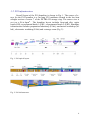
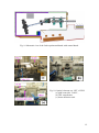
Overall layout of the P10 beamline is shown in Fig. 1. The source of xrays for the P10 beamline is a 5m long U29 undulator located in the low-beta
straight section of sector 7 of the PETRA III storage ring. The source size is
. The beamline layout includes front-end slits, optics
hutch (OH), experimental hutch 1 (EH1), experimental hutch 2 (EH2). Beamline
infrastructure includes preparation laboratory (P-lab), mechanical workshop (Mlab), electronics workshop (E-lab) and a storage room (Fig. 2).
Fig. 1: P10 optical layout.
Fig. 2: P10 infrastructure.
4
1.2.1. Optics hutch
The Optics Hutch (OH) is situated 33-46 m from the middle of the straight
section. There is some space available at the beginning of the optics hutch,
which is reserved for a high heat load flat mirror to enable pink beam operation
of the beamline. The standard PETRA III high heat load monochromator is the
next major component (Fig. 3a). It is located at ~38 m and cooled by liquid
nitrogen. Currently it is equipped with an independent Si(111) crystal pair (2.730.0keV) and an unpolished Si(111) channel-cut (7.0-17.0keV). In the future it
is planned to replace the independent Si(111) crystal pair with a Si(311)
channel-cut. Both channel-cuts will be polished. The channel-cut design offers a
much higher angular stability of the beam at the price of reduced energy ranges
and energy dependent exit offsets.
Next is a pair of flat (R > 100km) horizontally reflecting mirrors (Fig. 3b). The
mirrors are coated with a Rhodium and a Platinum stripe to match the cutoff
energy for higher energies to the experimental conditions. The mirrors are
followed by the bremsstrahlung shield (often termed beamstop) in the optics
hutch. The beamstop is a water-cooled Densimet collimator with holes for the
pink beam (4mm diameter) and the monochromatic beam (411 mm2). Both
beams need to be offset from the white beam position by a minimum of 20 mm.
A girder with several optical elements has been installed after the beamstop.
Site note: Currently the lowest reachable energy (~3.8keV) of the beamline is given by the
minimum gap of the undulator of 9.8mm.
It is foreseen to install the lens changer in the optics hutch of P10 (installation is
planned for the summer shutdown in 2013). The lens changer will be equipped
with vertical focusing (1D) Beryllium lenses (Fig. 3c). A total of 6 different lens
stacks will allow to match the horizontal and vertical transverse coherence
length at a 2nd lens changer in the experimental hutch. This focusing scheme
maximizes the available coherent flux for the experiment.
The 6 stacks will be equipped with the following lenses (number of lenses 
radius of lens curvature [mm]):
1) 8 x 0.5mm
2) 4 x 0.5mm
3) 2 x 0.5mm
4) 1 x 0.5mm
5) 2 x 1.5mm
6) 1 x 1.5mm
5
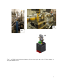
(a)
(c)
Fig. 3: (a) High heat load monochromator, (b) the mirror pair and (c) the 1D lens changer in
the optics hutch of P10.
6
1.2.2. Experimental hutch 1
EH1 is a 12m long hutch situated 67-79m from the source. Figure 4 shows the
experimental setups installed and foreseen in EH1. After some optical
components (explained in more detail below), three different sample
environments follow. First, a specialized setup for soft matter CDI/XPCS
experiments with a sample-to-detector distance of ~ 20 m and relatively large
beam sizes is installed. The accessible Q-range is limited (Q < 210-2Å-1 @
8keV), but the reduced flux density can be beneficial for many soft matter
systems. This sample environment is followed by the large 6-circle
diffractometer, which is currently under commissioning. Finally, a rheology
setup is installed which allows to conduct experiments in vertical scattering
geometry.
The first 3m of the hutch are dedicated to house a set of shared optical
components for the complete beamline (Fig. 5). The first element in EH1 is a
combination of beam positioning monitor (BPM) by FMBOxford and diamond
window situated on a granite block. The beam position is estimated from the
backscattered intensity of 0.5 µm thick foils (Titanium or Nickel). The water
cooled diamond window (5 mm diameter; 60µm thick) is connected to the BPM.
This is the only window of the beamline separating the ring vacuum from the
beamline vacuum.
These components are followed by an optical table that houses different optical
components. EH2 contains an identical optical table to allow sharing of optical
components between the experimental hutches. The first element is water cooled
slit system operated in closed loop with a maximum opening of 10x10mm2 and a
resolution of 0.2 µm. The second element is a dual fast shutter system for 2D
detectors. One system is based on amplified piezo actuators (similar to a design
by Cedrat; ~1ms) and the second system is based on magnetic coupling
(~30ms). This is followed by an absorber system and a retractable monitor unit
to check the beam intensity.
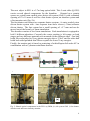
Shared optical components in EH1
The first component in the first experimental hutch EH1 is a FMB Oxford beam
positioning monitor (BPM). A water cooled diamond window (5 mm OD, 60
micron thickness) is connected downstream to the BPM. This device
combination sits on a granite post and can be aligned (vertical and horizontal) to
the beam using two Huber stages (Fig. 5a). The travel ranges allow to shift
between 'pink' and 'monochromatic' beam options. It is possible to stabilize the
beam position at the BPM using vertical and/or horizontal feedback programs.
7
The next object in EH1 is a 2.7m long optical table. This 5-axis table (Q-SYS)
carries several shared components for the beamline . Situated on a granite
spacer are a pink beam capable piezo driven slit system (Galil 1) with a nominal
opening of 10 10 mm2 as well as a fast shutter system, an absorber system and
a first monitor unit (Fig. 5b).
The fast shutter unit houses two separate shutter systems: A water-cooled, piezo
driven shutter system with ~1ms response time and a slower (~30ms) actuator
driven shutter. The fast system has a small opening of ~0.7 mm and can be
moved out of the beam by a linear translation.
The absorber consists of two linear translations. Each translations is equipped to
hold 9 different absorbers. Currently the center position is left empty on both
stages and two different materials are mounted on the different sides. One half
holds Silver absorber for X-ray photon energies above 12 keV and the other half
holds both sided polished thin Silicon crystals for lower X-ray energies.
Finally, the monitor unit is based on scattering of a thin Kapton foil under 45° in
combination with a Cyberstar scintillator detector.
Fig. 4: Schematics of the 1st experimental hutch (EH1) and control hutch (CH1) at P10.
(a)
Fig. 5: Shared optical components in the EH1: (a) BPM; (b) slit system Galil 1, fast shutter,
absorber unit and beam intensity monitor.
8
Soft matter CDI/XPCS setup of EH1
The setup for soft matter CDI/XPCS of EH1 (Fig. 6) is very similar to the
standard CDI/XPCS setup in EH2. It is mounted on a 5-axis optical table from
IDT. In front of the sample position, it features a pair of slit from JJ X-Ray (IBC30-HV). These slits are ~700mm apart. The first slit defines the size of the Xray beam and the second slit acts as a guard to suppress most of the slit
scattering of the first slit. Between the slits, an in-vacuum (retractable) monitor
unit is installed. The sample chamber is based on a DN100 (6" flange OD) UHV
cube. The cube is mounted on a 4-axis Huber tower (X, Y, Z and RZ). The
cube is fully vacuum integrated using DN (2.75" flange OD) bellows along the
X-ray beam direction.
Multiple different sample inserts have been developed to be housed in the
sample chamber (transmission and reflection setups, which are listed under
EH2/Standard Setup/Sample Inserts). The sample position is followed by a
DN100 (6" flange OD) 6-way cross. This 6-way cross allows e.g. to mount invacuum detector (e.g. diodes) as well as a vacuum pumping system. The last
piece of the sample environment is a DN100 gate valve before the scattered
signal is transported to the end of the hutch in a 4" ID tube. There the tube
diameter increases to 8" ID and the beam transport continues to the detector
stage in the 2nd experimental hutch. By using a detector position at the end of
EH2, a sample-to-detector distance of ~20 m is possible.
The setup is modular and it is envisioned that components can be removed from
the IDT 5-axis table to make room for more complicated experimental setups.
The optical table is equipped with a 1.51.0 m2 breadboard (mounting holes are
M6 on a 2525mm2 grid). All optical tables at P10 are designed to have a 600
mm distance between X-ray beam and table top surface.
Fig. 6: Soft matter CDI/XPCS/USAXS setup
of EH1.
9
Six-circle diffractometer
Experimental hutch EH1 is housing a large 6-circle Huber diffractometer (Fig.
7), which enables scattering/diffraction experiments at large scattering vectors
Q. The diffractometer is very similar to a diffractometer installed in the first
experimental hutch of P09. More detailed information will become available as
soon as the first standard components have been adapted to the diffractometer
environment.
Fig. 7: Huber 6-circle diffractometer.
Rheology setup
Finally, the experimental hutch EH1 houses a rheology setup (Fig. 8). This setup
allows to conduct experiments in vertical scattering geometry with a rheometerto-detector distance of ~3 m using a HAAKE rheometer.
Fig. 8: RheoSAXS setup.
10
1.2.3. Experimental hutch 2
The second experimental hutch EH2 is located at 83-95m from the X-ray source
(Fig. 9). It is home to the standard CDI/XPCS setup as well as to the holography
setup. Most experiments performed at Coherence Beamline P10 have the
sample located at ~87.8 m from the source. The standard setup and the
holography setup are movable on air pads and can be easily exchanged. Both
setups share an 5m long flight path as well as the motorized detector stage.
The optical table in EH2 carries a water cooled closed loop slit system
followed by a retractable monitor device to define the beam direction as well as
a micro-focusing lens changer (1D & 2D focusing capability) and a beam
deflection unit (BDU) to enable studies on liquid surfaces.
General components
The first element in experimental hutch EH2 is a DN200 (8" tube ID) gate valve,
which is not shown in the following. This page describes components which are
situated on a 2.7m long optical table in EH2. The 5-axis table is similar to the
optical table at the beginning of EH1. The table can be moved out of the beam to
install a DN200 (8" tube ID) flight tube, which allows to have a sample in EH1
and use the detectors in EH2.
A piezo drien water-cooled slit system (Galil 2) followed by a monitor unit are
sitting on a granite block at the start of the optical table in EH2 (Fig. 10a). The
maximum nominal slit opening is 10x10 mm2 and the resolution of the slit
position is 0.2 microns. Similar to EH1, the monitor unit is based on scattering
of a thin Kapton foil under 45° in combination with a Cyberstar scintillator
detector.
The beamline uses Beryllium lenses to reach focal spot sizes between 3-5
microns in both, vertical and horizontal, direction. The lens changer
(transfocator design) is equipped with 12 stacks of interchangeable Beryllium
lenses, which allows to have the correct lens combination for the desired focal
distances (of several meter) and for X-ray energies between 5-18 keV (Fig. 10b).
A Matlab macro can be used to calculate the best lens combination and best
lens-to-sample distance for the chosen X-ray energy.
The beamline has developed a beam deflection unit (BDU). The BDU uses two
Ge(111) crystals to slightly tilt the beam downwards (Fig. 10c). This enables
studies of liquid surfaces in grazing incidence conditions (i.e. no full
reflectivities up to large angles, but enough to reach incidence angles of up to 2x
the critical angle of most liquids). Details on the construction can be found in
the diploma thesis of Milenko Prodan and the apprenticeship report of Sergej
Bondarenko (both are in German).
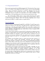
11
Fig. 9: Schematic view of the 2nd experimental hutch with control hutch.
Fig. 10: Optical elements on ‘OT2’ of EH2:
(a) pink beam slits ‘Galil 2’,
(b) CRL transfocator,
(c) beam deflection unit.
12
Standard CDI/XPCS setup at EH2
The standard CDI/XPCS setup in EH2 is based on a 2-circle Huber
diffractometer in horizontal geometry (Fig. 11a). This diffractometer is mounted
on a granite support and can be moved out of the beam path on air pads. The
diffractometer is based on a combination of a Huber 440 and 430 goniometer
sitting on a YZ translation. For most experiments the 440 goniometer is used as
the rotational bearing for the 5 m long detector arm. On top of the goniometers a
tower of Huber stages (170170mm2 size) is mounted. In the typical
configuration it offers XYZ translations (XY: Huber 5102.20; Z: Huber
5103.A20-40) as well as a 2-circle segment (Huber 5203.20) for rotations
around X & Y. A DN100 (6" flange OD) vacuum cube is used as the standard
cell for the sample environment. Examples for different sample cell inserts are
displayed when clicking on the navigation button (left side).
For experiments in SAXS geometry, the sample cell is fully vacuum
integrated. It is connected along the X-ray beam direction with DN40 (2.75"
Flange OD) bellows. Upstream of the sample environment sits a pair of JJ XRay slits (IB-C30-HV) on a Huber YZ stage. Between the slits is a vacuum
integrated monitor unit. Downstream of the sample environment a 6-way cross
(4" tube ID) followed by a DN100 gate valve connects the sample region via a 5
m long flight path to the detector region (Fig. 11b).
(a)
Fig. 11: (a) Schematic view of the standard
XPCS/CDI setup in EH2. (b) Schematics of the
standard sample setup integrated to the detector
stages.
(b)
13
Sample inserts
The main idea of using a DN100 vacuum cube as an experimental chamber is
the possibility to easily change between different experimental conditions. P10
has developed a set of standard sample inserts, but it should be easily possible to
design a sample insert for almost any arbitrary experimental condition.
Additional possibilities are e.g. a stress-strain insert. Fig. 12 shows the drawings
of currently available sample inserts.
(a
)
(b
)
(c
)
(d
)
Fig. 12: (a) The transmission sample insert. This insert allows to study samples in vacuum
sealed capillaries at temperatures in between 0 - 200 °C.
(b) The low temperature transmission sample insert. This insert covers a
temperature range in between -150 - 50 °C.
(c) The low temperature insert with an additional holder for small magnetic fields.
The holder is based on electromagnets and produces variable fields up to ~0.1 T.
(d) A sample insert for reflection experiments in a temperature range from 0 - 200
°C.
Nanofocusing setup at P10
The group of Prof. T. Salditt of University of Göttingen designed and installed
the experimental setup GINIX for holographic imaging at P10. The setup is
placed on a 5-axis table (IDT). This table is movable on air pads and can be
exchanged with the standard CDI/XPCS setup. Further details can be found in
1) Kalbfleisch, S., Neubauer, H., Krüger, S. P., Bartels, M., Osterhoff, M., Mai, D.
Giewekemeyer, K., Hartmann, B., Sprung, M. & Salditt, T. (2011). AIP Conf.
96-99.
D.,
Proc. 1365,
2) Kalbfleisch, S. (2012). PhD thesis, Georg-August-Universität Göttingen, Germany.
14
Flight path and detector stage
The detector stage in experimental hutch EH2 of P10 is based on a 3.5 m long
translation mounted on a granite block at the end of the experimental hutch (Fig.
13). The granite block is rotated by ~15° from the perpendicular direction to the
beam. This setup allows to rotate the 5m long flight path and detectors around
the sample position by ~30 degrees in the horizontal direction, which makes it
possible to perform coherent scattering experiments at large Q values (~2 Å-1 @
8keV). A set of different detectors currently in use at P10 is described in section
3.
Fig. 13: (a) View of the standard CDI/XPCS setup in EH2.
1.2.4 Support laboratories
Coherence Beamline P10 has three supporting laboratories: A mechanical
laboratory (P10-MLab), an electronic laboratory (P10-ELab) and a sample
preparation laboratory (P10-PLab). The names are an indicator of their main
use.
The mechanical laboratory is dedicated to preassembling of sample
environments, testing of vacuum windows and whatever tasks seems to fit. It is
equipped with a small working bench, a water sink, supply of compressed air
and some standard gases as well as cooling water.
The electronic laboratory is equipped with an additional electronic rack,
which includes a VME and a NIM crate. This allows testing of new motor stages
or detectors offline from the beamline. Again, cooling water, compressed air
and standard gases are available.
The sample preparation laboratory is not a full chemical laboratory, but it
allows simple tasks with harmless chemicals to be undertaken (e.g. cleaning of
vacuum components). Access to a fully equipped chemical laboratory can be
obtained via the DOOR system.
15
2. Starting the Experiment
2.1. Hutch search procedure
All areas of a beamline at PETRA III need to be searched before the x-ray
beam can be turned on. The purpose of the search is to make sure that nobody is
inside of the area when the x-ray beam is on. The interlock system of PETRA
III has developed a method for this purpose and this method will be described
here:
One user has to start the search procedure by placing a valid DACHS card
over the DACHS card reader (Fig. 14) near the “main” door (!!All other doors
and gates need to be closed in advance!!). This starts a warning message for the
area and activates the light barrier (which acts as a person counter) and the first
search button (a green button near the door) inside the area lights up. The user
proceeds by entering the hutch, searching the hutch and doing so pressing all
necessary search buttons (green buttons). After the user is finished with the
search the user returns to the hutch door and presses the yellow button near the
door to deactivate the light barrier for 5 seconds. Only then the user is able to
leave the area and to close the door. If the user has succeeded to follow this
procedure an orange light will come up near the door. The search is finished by
pressing the last “Final search” green button outside of the area followed by
placing the DACHS card over the DACHS card terminal again. An additional
red light will show up on top of the orange light. The warning message will
sound for a short moment before the “Permit Beam Operation” button gets
enabled on the Interlock Control System web page. Pressing this button locks
the doors and enables the “Open BS” button on the area panel.
Fig. 14: Interlock panel of P10 beamline
(OH).
16
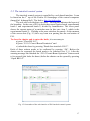
2.2. The interlock control system
The interlock control system is controlled by a web based interface. It can
be found on the 1st tap of the Firefox P10 homepage of the control computers
(haspp10e1 & haspp10e2). The link is: http://ics/index.php.
The web site is divided into two parts. The top part indicates the layout of
the beamline. In the case of P10 it shows three areas (optics hutch, experimental
hutch 1 and experimental hutch 2) divided by beamshutters. The lower panel
shows the current status of a particular area (in this case Area 3, which is the
experimental hutch 2). Clicking at the areas switches the panels. At the moment
of the screen shot (Fig. 15) the x-ray beam was passing into the end station of
P10.
To close the shutter and to enter the hutch, it is necessary to
a) press “Close BS 10.2”,
b) press “G 10.3 Cancel Beam Permission” and
c) unlock the doors by pressing “Break door interlock G10.3”.
Each of these actions needs to be confirmed by pressing “Ok”. Before the
shutter can be reopened the hutch needs to be searched (see 2.1.). After the
warning message has finished the “G10.3 Permit Beam Operation” button needs
to be pressed (this locks the doors) before the shutter can be opened by pressing
“Open BS10.2”.
Fig. 15: Screenshot of the web interface of P10 interlock control system.
17
2.3. Coordinate system at P10
P10 uses a right handed coordinate system, which is defined by the x-ray
beam direction. The 'X' axis is parallel to the beam direction, going to positive
values away from the x-ray source. The 'Y' axis is perpendicular to the beam
direction ('X') lying horizontal. The 'Y' axis goes to positive values outboard
from electron/positron accelerator ring. The 'Z' axis is perpendicular to the
beam direction ('X') standing vertical. The 'Z' axis goes to positive values from
the floor up.
Standard translation are called '..._X', '..._Y' & '..._Z'. The names is
derived by starting with a descriptive part followed by an underscore and the
following letter ('X', 'Y' or 'Z') indicates along which axis the translation is.
Standard rotation are called '..._RX', '..._RY' & '..._RZ'. The name is
derived by starting with a descriptive part followed by an underscore. The 'R'
indicates that it is a rotation and the following letter ('X', 'Y' or 'Z') indicates
which axis the rotation turns around. The sense of the positional values are
defined due to the fact that all rotations are right-handed (i.e. use the 'right hand
rule' from your undergraduate physics course).
Exceptions to this system will be explained on a case by case basis.
2.4. Preparing the beam
After the synchrotron beam is provided by the machine division (the
message on the PETRA III status panel has turned to ‘User Experiments’) one
can proceed to start the experiment as follows.
 First, all beamline hutches (optics hutch, experimental hutch 1,
experimental hutch 2) have to be set up (see §2.1).
 Next, one should close the undulator gap to the required value (16.3 mm
for photon energy of E=8 keV). This can be done by moving the virtual
motor ‘UNDULATOR’ in <ONLINE> GUI to the desired energy in [eV]
(Note, that for energies above 12 keV one has to use 3 rd harmonic of an
undulator, i.e. energy divided by a factor of 3 has to be applied). The
process of closing the undulator from ‘opened’ state to a ‘closed’ state
may take several minutes. During this time it is highly recommended not
to launch any other commands in <online> session.
 The motor ‘FMBEnergy’ (Bragg angle of double-crystal monochromator)
has to be also set to the required photon energy in eV.
 After closing the undulator gap one should wait for about 15 minutes until
the monochromator optics reaches the thermally stable state. After that
one can open safety shutter(s). Namely, all shutters in interlock GUI (Fig.
18
15, panel 10.1 – optics hutch, panel 10.2 – EH1, panel 10.3 – EH2) have
to be opened.
 The sizes of Galil slits G1 and G2 should be checked. These slits define
an optical axis for the whole beamline path and only horizontal and
vertical gap values need to be set (center positions should remain).
Usually the G1 is set to 0.6×0.6 mm2 and the G2 – to 0.3×0.3 mm2.
 If the undulator gap was set to a new setting it has to be scanned anew.
The ‘UNDULATOR’ virtual motor has to be scanned in a relevant range
and set to a peak position.
 In case the beamline was previously aligned, there should be already
beam intensity counted by the Cyberstar beam monitors in EH1 and EH2.
Usual command is
>osh; count; csh.
This command opens fast shutter, counts the intensity for 1 s and closes
fast shutter.
 Fine alignment of the monochromator is executed by the virtual motor
‘XTAL2_PITCH’ which should be scanned in a proper range (the stored
setting should normally be correct; in case of doubt please ask the local
contact). After a scan is finished the motor has to be set to a center-ofmass position.
 Next, the 2nd mirror should be scanned using the motor ‘MIR2RZ’ which
is a pitch angle for this mirror (default range should be right, otherwise a
range of ±0.002 deg. is sufficient). The position should be set to a centerof-mass value.
 After scanning the 2nd mirror, a monochromator pitch scan should be
repeated. After this is done the optical alignment is mainly completed and
the vertical beam position stabilisation should be turned on by launching
the python script ‘bpmcontrol.py’ located at the /beamline/macros/python/
folder on the experimental control PC (haspp10e1 or haspp10e2 for
experiments carried out at the EH1 or EH2, correspondingly). Note that
for repeating monochromator pitch the bpmcontrol.py script has to
disabled first.
 Further steps concern the alignment of JJ slits, focusing optics,
beamstops, detector and a sample, which will be described further in the
User Guide.
19
2.5. Sample mounting
The procedure of mounting/changing the sample depends on the type of
executed experiment. For in-vacuum sample mounting the first step is to vent
the sample area. After the venting is done, the sample can be changed. The last
step is evacuating of the sample cell.
How to vent and pump the sample area
The sample cell is connected to a turbo pump stage and two gate valves
can be used to separate the sample from the flight path before and after the
sample. To safely change a sample several steps are necessary and described
here:
1) Vent the sample cell:
1) Close both gate vales by turning the 'Output' of the HAMEG power
supply off
2) Press 'Stop' on the turbo pump touch panel
3) Press 'Open Vent' on the turbo pump touch panel
4) Open the manual vent valve near the sample cell slightly (2030mbar on P3) and wait for the turbo pump to spin down ~10.000
rpm
5) Fully open the manual valve and wait till the pressure is equalized
6) Remove the sample insert and change your sample
2) Pump the sample cell:
1) Remount the sample cell insert
2) Close the manual vent valve near the sample cell
3) Press 'Close Vent' on the turbo pump touch panel
4) Press 'Start' on the turbo pump touch panel
5) Wait until the pressure sensor P3 reads a pressure < 1e-03 mbar
6) Open both gate valves by turning the 'Output' of the HAMEG
power supply on
Now you are ready to search the hutch and start measuring your new
samples.
20
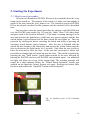
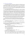
2.6. JJ X-ray slits calibration
The paragraph describes a procedure to calibrate the JJ X-Ray slits (pair
of slits in front of a sample, Fig. 10a) on a micro meter level. The first step for a
rough alignment should be to look at the beam with the x-ray eye. Use the macro
‘det xray’ The user should close the slit blades one by one roughly centered over
the beam on the x-ray eye. This way the user should produce a small square
beam on the x-ray eye display. Beam sizes smaller than 100 microns by 100
microns can easily produced this way.
Now change to the Cyberstar detector using the ‘det cbs’ macro (currently
Si diode inside the flight tube is used instead, command > diode in). Now the
user should close the slit by moving the top blade and perform an absolute scan
(~5 micron step size) towards positive values. In this direction the top blade has
no backslash. The scan should be flat in the beginning (close position) and start
to increase linearly at some point. After the scan is finished return to this
turning point and perform a fine scan (1 micron step size) around this position.
The turning point found during this fine scan should be used to set both the top
and the bottom blade to zero. Now the slit should be opened to ~50micrometers
in the vertical direction and the procedure should be repeated in the horizontal
direction. Here the slit needs to be closed by the left blade. The left blade in
than scan in positive direction without backslash as in the vertical direction.
Once the slit size is defined in both direction the slit center can be
scanned. The slit are setup in a way that the center scans are performed without
backslash. Once the center are found the positions of all four blades should be
reset.
The following example sequence of commands serves to adjust JJ X-ray
slits (SLT1, SLT2) using Si diode.
One of JJ X-ray slits, for instance SLT1, has to be fully opened (>
moveslit 1 2 0 2 0) while the other, SLT2, is getting adjusted. All the positions
mentioned further are in mm. Diode has to be in ( > diode in).
1) Adjust SLT2 horizontally by setting its size to 0.5 mm and check
transmitted intensity:
> moveslit 2 0.5 0 2 0; count
Make slit gap smaller until the transmitted intesity starts to decrease; at
this point one should roughly adjust the horizontal center (SLT, cx).
Slit down horizontal gap to 0.1:
> moveslit 2 0.1 0 2 0
and do scan of horizontal center:
ONLINE GUI: 'Scans' → 'Slit' → SLT2 → 'cx' ;
the range is 0.8 , number of points 41.
2) After the scan has finished, go to the center of the scanned maximum.
Next we scan the horizontal gap (SLT2 → dx) in a range -0.02 … 0.02
(note: JJ slits are made such that negative gaps are possible while the
blades can go behind each other without clashing). The last scan should
21
have a step-function profile. The point where intensity starts to linearly
increase is the actual 'zero' of horizontal gap. To calibrate both 'Left' and
'Right' blade positions one selects 'Properties' by right-click, then puts
'Register' to zero followed by 'Apply', and then one puts 'Position' to zero
also followed by 'Apply'. OK, with that horizontal gap is calibrated.
3) Now the vertical slit has to be adjusted. For that we open horizontal gap
to 0.4 and repeat steps 1)-3) for the vertical center (‘cy’) and gap (‘dy’).
To adjust the first slit SLT1 one has to open the SLT2 (> moveslit 2 2 0 2 0) and
follow steps 1) - 4).
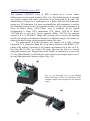
2.7. CRL transfocator alignment
The CRL x-ray transfocator based on beryllium CRLs is installed at the
EH2 at a distance of 86.1 m from a source. The CRLs with different curvature
radii (50 to 1000 m) are grouped in 12 stacks. The first 4 stacks contain 1D
lenses and the other 8 stacks contain 2D lenses. There are in total 212=4096
possible lens combinations. In order to select the best combination for a given
photon energy and image distance all possible combinations should be scrolled.
For this purpose a Matlab script was written which calculates the correct lens
combination as well as the optical parameters of a focused beam (offset
distance, focal spot size, efficiency, gain and depth of focus). The script is
available on the Windows analysis PC of EH2 control hutch. Start Matlab and
browse to the directory 'C:\Matlab\tools'. The script is called 'P10lens_v2' and
expects two input parameters, the x-ray energy in keV and the distance from
lens center to sample in meters. At the standard lens position this distance is
1.574 m. The Matlab call 'P10lens_v2(8.0, 1.574)' generates the following
output:
ans =
bestcombi: 768
bestbinary: [0 0 0 0 0 0 0 0 1 1 0 0]
bgoal: 1.5740
dist: -0.0489
bfinal: 1.6229
deltadist: -1.5616e-005
verticalsize: 2.5189e-007
horizontalsize: 1.5113e-006
bestefficiency: 78.2624
bestgain: 3.2894e+005
nstacks: 2
DOF_v: 0.1045
DOF_h: 0.1045
v_size_diff: 3.0788e-006
h_size_diff: 3.4204e-006
Note: all the output distances are in meters.
22
For transfocator alignment the following parameters are important:
 'bestcombi'. This parameter is the value needed to select the correct CRL
stack combination. These stacks are moved into the beam by typing the
command:
online> mva ehcrl bestcombi
The lens is moved out of the beam by typing ' online> mva ehcrl 0'.
 'dist'. This value describes an offset value for the motor 'ecrlx2'. This
motor moves the whole lens tower along the beam direction to bring the
focal spot to the sample. The command is
online> mva ecrlx2 dist
Here dist is an offset distance in mm.
During the transfocator alignment both JJ1 and JJ2 slits should be opened (1 × 1
mm² ). Alignment of the transfocator is done by scanning the whole device in
vertical and horizontal directions perpendicular to the beam (G2 should be set to
0.2×0.2 mm²). Corresponding motors ‘ecrly’ and ‘ecrlz’ should be scanned in a
relevant range (± 0.5 mm). Additionally the two tilts, ‘ecrlry’ and ‘ecrlrz’ have
to be used for final alignment of the transfocator axis (which should be parallel
to the beam).
Once these commands are executed, the G2 slit size should be set to 100 –
200 m vertically and 75 – 100 m horizontally (a trade-off opening of 150(V)
× 75(H) m² provides high spatial coherence at optimal coherent flux in a
focused beam). In addition the user can close the JJ2 slit to about 0.05 x 0.05
mm² around the beam for reduction of a background scattering.
23
3. Detectors at P10
The Coherence beamline P10 has several different detectors in use and it is
possible to reserve additional specialized detectors via the DESY detector pool:
o Pilatus 300K detector (Dectris),
487x619 pixels,
Pixel size of 172172 µm2.
o A Maxipix 2x2 detector (ESRF) is often is use at P10.
516x516 pixels,
Pixel size of 5555 µm2.
o As the 'work horse' 2D detector for XPCS / CDI experiments a PILCX detector (Princeton Instruments) is available. This slow direct
illumination CCD with a 2020 µm2 pixel size and 13401300
pixels has been used intensively at coherence beamlines around the
world.
o A Mythen 1K detector (PSI) is used as a fast 1D detector at P10,
having 1280 strips.
o As a point detector an avalanche photo diode (ESRF) is available in
combination with an hardware autocorrelator (Correlator.com).
3.1. PILATUS 300K
The PILATUS 300K detector is a 2D detector (developed by PSI and sold by
Dectris) with a pixel size of 172x172m2, 487x619 pixel active area, 20bit/pixel dynamic range and readout time of 7 ms. The quantum efficiency is
91% at 5.4 keV, 96% at 8 keV and 37% at 17.5 keV.
To start operating the Pilatus one has to proceed as follows:
1) From the experimental terminal in EH2
p10user@haspp10e2:~$> ssh –l det haspp10pilatus
> cd p2_det
> runtvx
2) Start Pilatus Tango server ‘Pilatus/P10E2’ from the Astor panel
3) Make sure the detector is ‘active’ (uncommented) in the online.xml file
4) restart <online> GUI
24
5) Setup working directory
<online> p300setup “directory” “name_of_file” 1
6) Use ‘p300take’ or ‘p300series’ commands to record images.
To start the P10 image viewer :
1)
p10user@haspp10e2:~$> cd /beamline/matlabmacros/
p10user@haspp10e2:~$> cp P10show2_pilatus300K.ini P10show2.ini
2)
Start image viewer GUI by double-clicking the desktop shortcut
‘Show Pilatus’
3)
Enter relevant file path and prefix; ‘Update’ button serves to view a
selected image.
3.2. MAXIPIX 2x2
The Maxipix detector in 2x2 configuration is a 2D detector developed at ESRF
which has a pixel size of 55x55m2, 516x516 px2 (28.4x28.4 mm2) active area,
dynamic range (count rate) of 100000 cps/pixel at 10% dead time and maximum
frame rate of 350 Hz (0.3 ms readout). The quantum efficiency is 100% at 8
keV, 68% at 15 keV and 37% at 20 keV.
In the following it is explained how the Maxipix detector is implemented
at the P10 beamline.
1) A 'ssh' connection to the Maxipix control computer needs to be established
via:
> ssh [email protected]
There exists an auto login from the experimental control computers ('haspp10e1'
or 'haspp10e2'). Please check at this point of the network storage of P10 is
mounted by testing the command 'cd /data'.
2) The program 'Dserver1' (5x1) or 'Dserver2' (2x2) needs to be started from the
command line on the Maxipix computer. Once these steps are finished, the
Maxipix device definitions can be activated in the 'online.xml' file and 'Online tki' can be called on the experimental control computer ('haspp10e1' or
'haspp10e2').
The Maxipix detector can now be controlled from 'Online' in a variety of
ways:
a) A widget has been created on the 'Online TKI Window' under
'Misc'.
b) Several Perl scripts are available to take a single image or a time
series of images.
c) The Maxipix detector has been implemented as virtual counter.
d) The Maxipix detector has been implemented into the XPCS
measurement scripts.
25
There are typical three Perl scripts (...setup, ...series and ...take) for 2D detector
operation at the P10 beamline. These can be called from the command line in
the following way:
1) 'max22setup “/network storage directory/” “filenamestart_”
firstframenumber'
2) 'max22series nframes exposuretime'
3) 'max22take exposuretime'
Note: The Tango server for the Maxipix detector loads by default an
incomplete configuration and it is advisable to run the setup script ('max51setup'
or 'max22setup') once at startup to define all necessary parameters.
3.3. PI-LCX
The LCX detector is a CCD detector (Princeton Instruments) with a pixel size of
20x20m2 , 1340x1300 pixel active area, 16-bit dynamic range (effective 5-6 bit
dynamic range) and readout time about 1.7s. The quantum efficiency is 75% at 5
keV, 50% at 8 keV and <5% at 12 keV.
The operation of the LCX camera from Online/Tango is not straight
forward. The momentary solution communicates via a Perl server script with
the Roper Scientific Winview software. This communication is one-sided,
meaning that Winview is not providing any information (output) about its status.
This means, that the Tango/Online control has to be very careful. Any error
message in Winview will cause severe problems which will need several steps to
recover (up to restart Winview + Perl Server and Tango Server!).
The WinView program is installed on ‘haso052lcx.desy.de’ and the
account ‘lcxuser’ should be used. Before launching the Winview software
(shortcuts can be found on the desktop and the quick launch toolbar), the PILCX camera should be connected to the ST133 camera controller, which can be
sub-sequentially turned on. The next step involves mounting the network
storage. The network storage drive is mounted as disk Y:\. It must be mounted
from the p10user!
After launching the Winview software the cooling for the CCD chip
should be turned on and be set to -40degC. This can be done in Winview under
‘Setup/Detector temperature’. Also, the image orientation should be set under
‘Setup/Hardware’ on the display tab. The 'Reverse' and 'Flip' flag should be set.
Once these steps are finished the Perl server program ‘lcx_xpcs_server.pl’
must be launched by clicking the shortcut ‘StartPerlServer.bat’ (again on the
desktop or on the quick launch toolbar). The Perl server program as well as the
other Perl scripts can be found in ‘D:\Perl\’. The file ‘StartPixisPerlServer.bat’
should be used for the PIXIS detector.
Now all necessary steps on ‘haso052lcx’ are finished and the user should
restart the Tango Server ‘LCXCamera/P10E2’ to re-establish the
communications.
26
The Perl Server can read and write the following attributes, 1)
SavingPath, 2) FileNameStart, 3) FirstFrame, 4) NumFrames, 5) ExpTime, 6)
DelayTime as well as the following commands 1) Go and 2) Status.
The ‘Go’ command starts a series of ‘NumFrames’ frames with the
exposure time ‘ExpTime’ and the delay time ‘DelayTime’ between frames.
Both 'time' parameters are in seconds. The data are stored under ‘SavingPath’
with the file name constructed by ‘FileNamestart’ followed by a 4 digit frame
number. The frame numbering starts with ‘FirstFrame’ and the images are stored
as ‘*.spe’ files.
If ‘NumFrames’ is smaller or equal to 256 and the ‘DelayTime’ is set to
zero than the data are stored in multi image files. This has the advantage that an
additional overhead between frames of ~0.6seconds can be prevented. The time
between frames for a full frame exposure can be estimated as: Readout time
(1.8s) + ‘ExpTime’ + ‘DelayTime’ + Overhead (0.6s).
3.4. PI-Pixis
The Pixis detector (Princeton Instruments) is a new generation of CCD detector
from Princeton Instruments having mainly the same as in LCX CCD chip
installed (pixel size 20x20m2 , 1340(h)x1300(v) px2 ). The detector requires no
water cooling circle, otherwise the installation procedure is same as in the LCX
case.
3.5. Andor iKon-L
The Andor iKon-L is a high resolution CCD camera with chip area of
20482048 px2 and pixel size of 13.513.5 m2 . Readout frequency up to 5
MHz is possible with this detector. In order to operate the peltier-cooled chip
working at -65 C , the camera requires water cooling cycle ( normal setting of
15 C). The Andor camera acquires images (tif, edf) with 16-bit resolution.
27
4. Recovery steps in case of computer failures
General information
The P10 beamline is controlled by a Linux based computing system.
Each area of P10 has its own control computer. These computers are called:
1) Optics hutch:
haspp10opt
2) Experimental hutch #1: haspp10e1
3) Experimental hutch #2: haspp10e2
Each of these computers controls hardware via an independent VME controller
and an independent Tango Device Manager (called by 'astor').
Additionally the P10 beamline has 2 more control computers:
1) P10 E-Lab:
haspp10lab
2) Vacuum interlock PC: hasp10vil
Some possible scenarios
The users will use ONLINE to control their experiments most of the time.
So if ONLINE hangs than it should be restarted first. In general the instruction
manuals to ONLINE and other experimental control software can be found on
the web pages of FS-EC under computing manuals:
http://hasylab.desy.de/infrastructure/experiment_control/index_eng.html
Terminating 'Online'
To kill 'Online' open a new terminal and type:
> ps a | grep gra_main
This command searches for the process identity ('pid') of the ONLINE process.
This process identity is listed in the first column. Try to kill the ONLINE
process by typing: kill -1 pid
If the process persists use the more brutal command:
kill -9 pid
After ONLINE has been terminated, it can be restarted by switching to the
ONLINE
data
directory
(normally
something
like:
'/data/YEAR+CYCLE/DATE/' and typing: 'online -tki' ).
Terminating Tango Servers
Please read the description for the ASTOR Tango Device Manager. It
explains how Tango Servers are killed and restarted.
Generally, one can try ‘Stop All’ (see Fig. 16), wait until all servers shut
down (turn ‘red’) and then ‘Start All’ (it takes several minutes until all servers
get on, i.e. ‘green’).
28
Fig. 16: Dialog window of the Astor Tango server manager.
Note:
If the above steps did not solve the problems then it might be necessary
to reboot the VME and/or the control computers. However, the previous
steps should always be tried first!
Rebooting the VME crate
In order to restart the VME crate, the Tango Servers of all, to the VME
connected, devices should be stopped. Looking at this screen shot (Fig. 16), the
'Stop All' button should be used. It is necessary to wait until all green indicators
are turned red, before proceeding to restart the VME. The VME is stopped by
turning the 'power off' of the fan unit underneath the VME (see Fig. 17). After a
10 second waiting time, the VME power can be switched back on and the Tango
Server can be restarted by using the 'Start All' button.
Fig. 17: View of the VME crate.
29
Restarting the control computer
If the control computer is frozen, then it might need to be reset. Before
using the hardware reset switch, one can try to use another control computer of
the P10 beamline to 'ssh' into the problematic control computer, e.g. opening a
new terminal and typing:
> ssh haspp10opt (e1 or e2)
The shutdown command would be:
> sudo /sbin/restart -P now
If this doesn't work the square 'reset' button under the front cover should be
used. Hopefully the computer comes up normally and the user can login as
'p10user'. The password should have been provided at the start of the beamtime.
Restoring the control computer
After the control computer is restarted and the user logged back on as
'p10user' it is necessary to recover the session. The p10 control computer has in
the standard configuration six desktop panels which can be accessed from the
taskbar located on the bottom of the screen. The six panels are called: 'Online',
'Optics', 'X-Ray Eye', 'Interlock', 'Macros' and 'Other'.
The Online panel
In this panel the ONLINE session and the Tango Device Manager for
EH1 & EH2 should run. It is recommended to open three terminals. The first
terminal should just start a Tango Device Manager. The command is: 'astor &'.
The second terminal should connect to the other control computer via ssh. The
command is: 'ssh haspp10e1' or 'ssh haspp10e2' depending on which control
hutch is occupied. The Tango Device Manager is called again by 'astor &'. The
third terminal should be used to call ONLINE. The user should first change to
the data collection directory (the standard directory would be of the form
'/data/YEAR+CYCLE/DATE/'). ONLINE is started then by typing 'online -tki'.
The Optics panel
This panel should be used to control components connected to the optics
control computer 'haspp10opt'. Again the user should open two terminals and
use both to ssh to the optics computer via: 'ssh haspp10opt'. The first terminal
should be used to start the Tango Device Manager via 'astor &' and the second
terminal should be used to open 'Jive' via 'jive &'. From the Jive panel the user
should open the Undulator control window. This can be done by opening the
tree 'Petra3Undulator', 'p10' and 'Petra3Undulator' till the 'p10/undulator/1'
device is found. A right click on 'p10/undulator/1' opens a context menu and the
selection 'Monitor Device' opens the undulator control window.
30
The Interlock panel
This panel should be used to start Firefox browser. The homepage of
Firefox is set to the following tabs:
Tab 1: Interlock control system
Tab 2: Vacuum interlock control system
Tab 3: PETRA III infoscreen
Tab 4: PETRA III machine log book
The X-Ray Eye panel
This panel is used to start the 'X-ray Eye' beam camera. The software for
the ‘X-ray Eye’ is installed on the optics control computer so it is necessary to
open a terminal and to use 'ssh haspp10opt'. The ‘X-ray Eye’ software is started
by typing 'SampleViewer' (case sensitive!). This opens the control window and
by clicking on the 'Eye' symbol the camera display window is opened and by
clicking on the 'Wrench' symbol the settings window is opened.
The other panels are currently not used.
31
5. Commands and macros at P10
To start the Online GUI interface (PerlTk interface) one has to launch
[p10user@hasp10e2]$ online –tki
from a Linux terminal on control PC (example of EH2).
Once the ONLINE session is started the control commands can be
executed from a command line of GUI. In following the commonly used macrocommands (syntax emulating SPEC commands) are listed.
Counting commands:
> count exptime
- execute acquisition by selected counters
for ‘exptime’ in seconds;
> diode in
- move photodiode (inside flight tube) in
the beam;
- extract photodiode from the beam;
> diode out
> refdiode in
> refdiode out
> udiode in
> udiode out
- move reference photodiode (after the
sample) in the beam;
- extract reference diode (after the
sample) from the beam;
- move USAXS photodiode (EH1) in the
beam;
- extract USAXS photodiode from the
beam;
Interlock shutter control macros:
Here ‘ehN’ means either ‘eh1’ or ‘eh2’ for experimental hutch 1 or 2,
respectively.
> ish ehN open
- open interlock shutter (usually after the
interlock is set by searching the hutch);
> ish ehN close
- close interlock shutter without breaking
the door interlock;
> ish ehN break
- close interlock shutter and break the
door interlock. Before entering the hutch
be sure the door lights are switched off;
Commands to control slow and fast shutters:
> osh
- open fast shutter;
32
> csh
- close fast shutter;
> oss
- open slow shutter;
> css
- close slow shutter;
> fastshutter in
- insert fast shutter in the beam path;
> fastshutter out
- extract fast shutter from the beam path;
Absorber commands:
> abs?
> abs n
> abs 0
Caution:
- show currently used absorber set; all possible
absorber combinations are also displayed;
- insert absorber in the beam, n is an integer
number from 0 to 192 ( possible number of 25
um thick Si plates/ Au foils: (0, 1, 2, 3, 4, 6, 8,
9, 12, 16, 18, 24, 32, 33, 36, 48, 64, 66, 72, 96,
128, 129, 132, 144, 192));
- move absorbers out (no absorber in the beam,
use with care!);
When working with 2D detectors, be sure to have fastshutter
inserted in the beam (‘>fastshutter in’)!
Commands to move/scan motors:
> wm mot1 mot2 mot3 … - display current position of a specific
motor (can be applied to up to 6 motors
simultaneously;
> mva mot1 x1
- move absolute motor ‘mot1’ to position ‘x1’
> mva mot1 x1 mot2 x2 mot3 x3 ...
- Move absolute a maximum
number of 6 motors simultaneously;
> mvr mot1 x1
- move relative motor ‘mot1’ to position ‘x1’
> mvr mot1 x1 mot2 x2 mot3 x3 ...
- Move relative a maximum
number of 6 motors simultaneously;
> whereslit n
- display the positions of blades of JJ slit ‘n’.
n=1, 2 or 3 correspond to JJ1, JJ2 ( pair of
collimating slits before a sample) and JJ3
(‘detector slits’ in front of CyberStar/APD);
> moveslit n hgap hcenter vgap vcenter
- move JJ slit ‘n’ (n=1, 2 or 3 ) to horizontal gap
‘hgap’, horizontal center ‘hcenter’, vertical gap
33
to ’vgap’ and vertical center of ‘vcenter’; all
target values are in [mm];
> ascan mot1 x1 x2 npoints ctime
- absolute scan of a motor ‘mot1’ from position
‘x1’ to position ‘x2’ with number of points
‘npoints’ and exposure ‘ctime’;
> dscan mot1 x1 x2 npoints ctime
- relative scan of a motor ‘mot1’ from position
‘x1’ to position ‘x2’ with number of points
‘npoints’ and exposure ‘ctime’;
> amesh mot1 x1 x2 NP1 mot2 y1 y2 NP2 ctime
- absolute mesh scan of motor ‘mot1’ in a range
from ‘x1’ to ‘x2’ with ‘NP1’ points at different
positions of motor ‘mot2’ in a range from ‘y1’
to ‘y2’ with ‘NP2’ points at exposure time
‘ctime’;
> dmesh mot1 x1 x2 NP1 mot2 y1 y2 NP2 ctime
- relative mesh scan ;
In case the motor movement/scan has been stopped (by pressing ‘Stop’ button in
ONLINE GUI), for restoring the ability to move motors, one needs to execute
the command :
> reset_stop
Commands to move the selected detector in its working position:
> det cbs
- move in the point detector (CyberStar/APD);
> det xray
- move in the ‘X-ray Eye’ camera;
> det max22
- move in the MAXIPIX (2x2) detector;
> det lcx
- move in the LCX CCD detector;
> det pixis
- move in the Pixis CCD detector;
> det p300
- macro command to move in the PILATUS
300K detector;
In the case when count command (for monitoring beam intensity with the
flight tube diode, diode in;) is used after previous use of 2D detector
(LCX/Pixis , Maxipix, or Pilatus) , one has to take over fastshutter control by
applying a macro command(s)
> ccd1off
# to take over from LCX/Pixis detector;
> ccd2off
# to take over from Maxipix detector;
34
> ccd3off
# to take over from Pilatus detector;
Commands for 2D detector acquisition:
Before starting acquisition with 2D detector one has to setup the detector by
> detsetup “/filedir/” “filename_” startnum ;
where
‘det’ stands for ‘p300’ (Pilatus300K detector), ‘max22’ (Maxipix
detector), ‘lcx’
(LCX detector) or ‘pixis’ (Pixis detector);
‘filedir’ is the directory where the data will be stored;
‘filename’ is the file root name;
‘startnum’ is the number of 1st frame.
> dettake exptime
- acquire a single frame with exposure time
‘exptime’ in seconds;
> detseries numframes exptime (delaytime) - acquire a series of
‘numframes’ frames with with exposure time
‘exptime’ and optional delay time in seconds;
Mesh scans with 2D detectors:
> detamesh mot1 x1 x2 NP1 mot2 y1 y2 NP2 nframes ctime
- absolute mesh scan with two motors and
acquisition by 2D detector;
> detdmesh mot1 x1 x2 NP1 mot2 y1 y2 NP2 nframes ctime
- relative mesh scan with two motors and
acquisition by 2D detector;
Operating the CRL transfocator:
> wm ehcrl
- display the currently used CRL combination;
> mva ehcrl <combi> - insert the lens combination combi in the beam
> mva ehcrl 0
> mva ehcrl 4095
> mva ecrlx2 dist
(read also §2.7);
- extract CRLs from the beam path;
- insert all CRLs in the beam path (for testing
only);
- move absolute the CRL transfocator along the
beam to the position dist in [mm];
DAC control:
> p10dac dacchannel voltage - set voltage in [V] to a
selected DAC channel (i.e. e2_dac03);
35
Lakeshore temperature controller commands:
> lake on;
- start LakeShore controller;
> lake off;
- stop LakeShore controller;
> lake pow <P>;
- set heater power level;
Possible values are 0, 1, 2, 3, 4, 5 which
correspond to heater power of 10 mW,
100 mW, 1 W, 10 W, 92 W;
> lake T ?;
- show actual temperature ;
> lake T ? A K;
- show actual temperature of channel ‘A’
in [K];
> lake T ? B C;
- show actual temperature of channel ‘B’
in [C];
> lake setp <T>;
- set setpoint temperature;
> lake PID <P> <I> <D> - set PID parameters of temperature
control (see LakeShore manual);
When using sample inserts equipped with Peltier element, one has to
switch on the Kepko current supply and set correct DAC voltage.
For heating above 100 C one has to apply command :
> p10dac e2_dac02 -2 ; # this command applies -2V voltage to
DAC channel e2_dac02, which converts
to -1.6 A current setting of Kepko supply.
For RT measurement and cooling down below RT one has to apply
following DAC voltages :
> p10dac e2_dac02 0.5 ; # for T range 285 – 305 K
> p10dac e2_dac02 1 ;
# for T range 270 – 290 K
> p10dac e2_dac02 0 ;
# for T range 300 – 350 K
36
Notes, comments:
___________________________________________________________________________
___________________________________________________________________________
___________________________________________________________________________
___________________________________________________________________________
___________________________________________________________________________
___________________________________________________________________________
___________________________________________________________________________
___________________________________________________________________________
___________________________________________________________________________
___________________________________________________________________________
___________________________________________________________________________
___________________________________________________________________________
___________________________________________________________________________
___________________________________________________________________________
___________________________________________________________________________
___________________________________________________________________________
___________________________________________________________________________
___________________________________________________________________________
___________________________________________________________________________
___________________________________________________________________________
___________________________________________________________________________
___________________________________________________________________________
___________________________________________________________________________
___________________________________________________________________________
___________________________________________________________________________
37