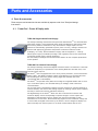
1
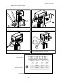
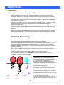
TELEDYNE
HASTINGS
INSTRUMENTS
INSTRUCTION MANUAL
HFM-I-401 AND HFM-I-405
INDUSTRIAL
FLOW METERS
-i-
Manual Print History
The print history shown below lists the printing dates of all revisions and addenda created for
this manual. The revision level letter increases alphabetically as the manual undergoes
subsequent updates. Addenda, which are released between revisions, contain important change
information that the user should incorporate immediately into the manual. Addenda are
numbered sequentially. When a new revision is created, all addenda associated with the
previous revision of the manual are incorporated into the new revision of the manual. Each new
revision includes a revised copy of this print history page.
Revision A (Document Number 171-042008) .......................................................................March 1999
Visit www.teledyne-hi.com for WEEE disposal guidance.
Description of Symbols and Messages used in this manual
WARNING
This indicates a potential personnel hazard. It calls attention
to a procedure, practice, condition or the like, which, if not
correctly performed or adhered to, could result in injury to
personnel.
CAUTION
This indicates a potential equipment hazard. It calls attention
to an operating procedure, practice, or the like, which, if not
correctly performed or adhered to, could result in damage to
or destruction of all or part of the product.
NOTE
This indicates important information. It calls attention to a
procedure, practice, condition or the like, which is worthy of
special mention.
Teledyne Hastings Instruments reserves the right to change or modify the design of its
equipment without any obligation to provide notification of change or intent to change.
- ii -
General Information
Quick Start Instructions
Connect dry, clean gas and ensure connections are
leak free.
Connect Cable for power and analog signal output.
Check that electrical connections are correct.
(See diagrams below)
Replace front cover and cable feed-through ensuring
gasket is seated and fasteners are secure.
12
1
Terminal Strip
+
-
PU
VS
P+
U
VS T
U
O
A
T+
U
O
A
IN
3
IN
4
A
2
A
M
O
C
D
O
R
ZE
1
M
AR
AL
2
M
AR
AL
M
AR
AL
Digital Connector
1
PINS
RS232
RS485
ETHERNET
SHIELD
1
2
3
4
GROUND
TRANSMIT
RECEIVE
UNUSED
UNUSED
GROUND
TX+ (A)
RX+ (A)
TX- (B)
RX- (B)
GROUND
TD+
RD+
TDRD-
For detailed set up instructions, see Section 2-Installation
- iii -
CAUTION
CAUTION
NOTE
This instrument is available with multiple pin-outs.
Ensure electrical connections are correct.
The 400-I series flow meters are designed for IEC
Installation/Over voltage Category II – single phase receptacle
connected loads.
The Hastings 400 Series flow meters are designed for
INDOOR and OUTDOOR operation.
CAUTION
In order to maintain the integrity of the Electrostatic Discharge
immunity both parts of the remote mounted version of the
HFM-I-400 instrument must be screwed to a well grounded
structure.
CAUTION
In order to maintain the environmental integrity of the
enclosure the power/signal cable jacket must have a diameter
of .157 - .315” (4 – 11 mm). The nut on the cable gland must
be tightened down sufficiently to secure the cable. This cable
must be rated for at least 85°C.
- iv -
General Information
Table of Contents
GENERAL INFORMATION.....................................................................................................................................1
1. GENERAL INFORMATION ....................................................................................................................................1
1.1. OVERVIEW......................................................................................................................................................1
1.1.1.
400 Series Family ..................................................................................................................................1
1.1.2.
400 Series Meters ..................................................................................................................................1
1.1.3.
Measurement Approach.........................................................................................................................1
1.1.4.
Additional Functions..............................................................................................................................2
1.2. SPECIFICATIONS .............................................................................................................................................2
INSTALLATION.........................................................................................................................................................4
2. INSTALLATION ....................................................................................................................................................4
2.1. RECEIVING INSPECTION ..................................................................................................................................4
2.2. ENVIRONMENTAL AND GAS REQUIREMENTS ..................................................................................................4
2.3. MECHANICAL CONNECTIONS .........................................................................................................................4
2.4. MOUNTING THE ELECTRONICS REMOTELY .....................................................................................................5
2.5. ELECTRICAL CONNECTION .............................................................................................................................5
2.5.1.
Power Supply .........................................................................................................................................6
2.5.2.
Analog Output........................................................................................................................................6
2.5.2.1.
Current Loop Output .........................................................................................................................6
2.5.2.2.
Voltage output....................................................................................................................................8
2.6. DIGITAL CONNECTION ....................................................................................................................................8
2.7. DIGITAL CONFIGURATION ..............................................................................................................................8
2.7.1.
RS-232 ...................................................................................................................................................8
2.7.2.
RS-485 ...................................................................................................................................................9
2.7.3.
Ethernet .................................................................................................................................................9
2.8. ALARM OUTPUT CONNECTION .....................................................................................................................10
2.9. AUXILIARY INPUT CONNECTION ..................................................................................................................11
2.10.
ROTARY GAS SELECTOR...........................................................................................................................11
2.11.
ELECTRICAL REMOTE ZERO CONNECTION ...............................................................................................11
2.12.
CHECK INSTALLATION PRIOR TO OPERATION ...........................................................................................12
OPERATION.............................................................................................................................................................14
3. OPERATION ......................................................................................................................................................14
3.1. ENVIRONMENTAL AND GAS CONDITIONS .....................................................................................................14
3.2. INTERPRETING THE ANALOG OUTPUT ..........................................................................................................14
3.3. DIGITAL COMMUNICATIONS .........................................................................................................................14
3.3.1.
Digitally Reported Flow Output ..........................................................................................................15
3.3.2.
Digitally Reported Analog Input..........................................................................................................15
3.4. ZEROING THE INSTRUMENT ..........................................................................................................................15
3.4.1.
Preparing for a Zero Check.................................................................................................................15
3.4.2.
Adjusting Zero .....................................................................................................................................16
3.5. HIGH PRESSURE OPERATION ........................................................................................................................16
3.5.1.
Zero Shift .............................................................................................................................................16
3.5.2.
Span Shift.............................................................................................................................................16
3.6. WARNINGS/ALARMS ....................................................................................................................................17
3.7. MULTI-GAS CALIBRATIONS ..........................................................................................................................17
3.8. FLOW TOTALIZATION ...................................................................................................................................18
3.9. ADDITIONAL DIGITAL CAPABILITIES ............................................................................................................18
PARTS AND ACCESSORIES .................................................................................................................................19
4. PARTS & ACCESSORIES .....................................................................................................................................19
4.1. POWER POD – POWER & DISPLAY UNITS ......................................................................................................19
4.2. FITTINGS.......................................................................................................................................................20
4.3. CABLES ........................................................................................................................................................20
WARRANTY .............................................................................................................................................................21
5.
WARRANTY ......................................................................................................................................................21
-v-
5.1.
5.2.
WARRANTY REPAIR POLICY .........................................................................................................................21
NON-WARRANTY REPAIR POLICY ................................................................................................................21
APPENDICES............................................................................................................................................................22
6. APPENDICES .....................................................................................................................................................22
6.1. APPENDIX 1- VOLUMETRIC VERSUS MASS FLOW .........................................................................................22
6.2. APPENDIX 2 - GAS CONVERSION FACTORS ...................................................................................................23
- vi -
General Information
1. General Information
1.1. Overview
1.1.1. 400 Series Family
The Hastings 400 Series is a family of flow instruments which is specifically designed to meet
the needs of the industrial gas flow market. The “I” family in the 400 Series features an IP-65
enclosure which allows the use of the instrument in a wide variety of environments. The 400 I
products consist of four configurations: a flow meter, HFM-I-401, which has a nominal nitrogen
full scale between 10 SLM and 300 SLM and a corresponding flow controller, the HFC-I-403; a
larger flow meter, HFM-I-405, which ranges from 100 SLM to 2500 SLM, and a corresponding
flow controller, the HFC-I-407. These instruments are configured in a convenient in-line flowthrough design with standard fittings. Each instrument in the series can be driven by either a
+24 VDC power supply or a bipolar ±15 volt supply. The electrical connection can be made via
either a terminal strip located inside the enclosure or optionally through an IP-65 compatible
electrical connector. Also, these instruments include both analog and digital communications
capabilities.
1.1.2. 400 Series Meters
The Hastings HFM-I-401 and HFM-I-405 thermal mass flow meters are designed to provide very
accurate measurements over a wide range of flow rates and environmental conditions. The
design is such that no damage will occur from moderate overpressure or overflows and no
maintenance is required under normal operating conditions when using clean gases.
1.1.3. Measurement Approach
The instrument is based on mass flow sensing. This is accomplished by combining a high-speed
thermal transfer sensor with a parallel laminar flow shunt (see Figure 1-1). The flow through
the meter is split between the sensor and shunt in a constant ratio set by the full scale range.
The thermal sensor consists of a stainless steel tube with a heater at its center and two
thermocouples symmetrically located upstream and downstream of the heater. The ends of the
sensor tube pass through an aluminum block and into the stainless steel sensor base. With no
flow in the tube the thermocouples report the same elevated temperature; however a forward
flow cools the upstream thermocouple relative to the downstream. This temperature
difference generates a voltage signal in the sensor which is digitized and transferred to the
main processor in the electronics enclosure. The processor uses this real-time information and
the sensor/shunt characteristics stored in non-volatile memory to calculate and report the
flow.
To ensure an inherently linear response to flow, both the thermal sensor and the shunt have
been engineered to overcome problems common to other flow meter designs. For example,
nonlinearities and performance variations often arise in typical flow meters due to pressurerelated effects at the entrance and exit areas of the laminar flow shunt. Hastings has designed
the 400 Series meters such that the flow-critical splitting occurs at locations safely downstream
from the entrance effects and well upstream from the exit effects. This vastly improves the
stability of the flow ratio between the sensor and shunt. The result of this design feature is a
better measurement when the specific gravity of the flowing medium varies, for instance due
to changes in pressure or gas type. Also, a common problem in typical flow meters is a slow
response to flow changes. To improve response time, some flow meter designs introduce
impurities such as silica gel. Alternatively, Hastings has designed the 400 Series sensor with
reduced thermal mass to improve the response time without exposing additional materials to
the gas stream.
-1-
1.1.4. Additional Functions
These instruments contain a number of functions in addition to reporting flow which include:
•
Settable alarms and warnings with semiconductor switch outputs
•
A digitally reported status of alarms and warnings such as overflow/underflow
•
A flow totalizer to track the amount of gas added to a system
•
A digitizing channel for an auxiliary analog signal
•
An internal curve fitting routine for “fine tuning” the base calibration
•
An alternate calibration set of 8 different ranges/gases
1.2. Specifications
Do not operate this instrument in excess of the specifications
listed below. Failure to heed this warning can result in serious
personal injury and/or damage to the equipment.
WARNING
HFM-I-401
Performance
Full Scale Flow Ranges
(in N2)
Accuracy1
Repeatability
Operating Temperature
Warm up time
Settling Time/Reponse
Time
Temperature Coefficient
of Zero
Temperature Coefficient
of Span
Operating Pressure Maximium
Pressure Coefficient of
Span
Pressure Drop([email protected]
psia)
Attitude Sensitivity of
Zero
HFM-I-405
0-10 slm up to 0-350 slm
Standard: ± 1% full scale
Optional: ± (0.5% reading + 0.2%FS)
± 0.1% of F.S.
-20 to 70°C
30 min for optimum accuracy
2 min for ± 2% of full scale
0-100 slm up to 0-2500 slm
Standard: ± 1% full scale
Optional: ± (0.5% reading + 0.2%FS)
± 0.1% of F.S.
-20 to 70°C
30 min for optimum accuracy
2 min for ± 2% of full scale
< 2.5 seconds (to within ± 2% of full scale)
< 2.5 seconds (to within ± 2% of full scale)
< ±0.05% of Full Scale /°C
< ±0.05% of Full Scale /°C
< ±0.16% of reading/°C
< ±0.16% of reading/°C
Standard: 500 psig
Optional: 1500 psig
Standard: 500 psig
Optional: 1000 psig
< 0.01%of reading /psi
(N2, 0-1000 psig)
< 0.01%of reading /psi
(N2, 0-1000 psig)
< 1.1 psi at full scale flow
< 5.1 psi at full scale flow
< 2% of F.S.
< 2% of F.S.
Power Requirements
Analog Output
18-38 VDC, 3.5 watts(Ethernet) 2.5
watts(RS232/485)
Standard: 4 – 20 mA
18-38 VDC, 3.5 watts(Ethernet) 2.5
watts(RS232/485)
Standard: 4 – 20 mA
Digital Output
Optional: 0-10 VDC, 0-20 mA, 0-5 VDC, 1-5 VDC
Standard: RS 232
Optional: 0-10 VDC, 0-20 mA, 0-5 VDC, 1-5 VDC
Standard: RS 232
Optional: RS 485
Optional: Ethernet
Std: Terminal Block – PG 9 Cable Gland
Optional: 12 pin Circular Connector
Optional: RS 485
Optional: Ethernet
Std: Terminal Block – PG 9 Cable Gland
Optional: 12 pin Circular Connector
Electrical
Analog Connector
-2-
Digital Connector
4 pin, D-coded M12
4 pin, D-coded M12
Standard: 1/2" Swagelok
Optional: ½" VCO®, ½" VCR®, ¾” Swagelok,
Standard: 1" Swagelok
Optional: 1" VCO®,1" VCR®, ¾” Swagelok, ,
10mm Swagelok, 3/8" male NPT, ½” male NPT
1" male NPT, ¾” male NPT, 1 5/16"-12 straight
12mm Swagelok, ¾"-16 SAE/MS straight thread
< 1x10⁻⁸ sccs He
316L SS, Nickel 200, 302 SS, Viton®
12 lb (5.5 kg)
thread
< 1x10⁻⁸ sccs He
316L SS, Nickel 200, 302 SS, Viton®
18 lb (8 kg)
Mechanical
Fittings
Leak Integrity
Wetted Materials
Weight (approx.)
Viton® is a trademark of DuPont Dow Elastomers, LLC.
Swagelok®, VCO®and VCR® are trademarks of the Swagelok Company.
-3-
Installation
2. Installation
CAUTION
Many of the functions described in this section require
removing the enclosure front plate. Care must be taken when
reinstalling this plate to ensure that the sealing gasket is
properly positioned and the fasteners are secure to maintain
an IP65 compliant seal.
2.1. Receiving Inspection
Your instrument has been manufactured, calibrated, and carefully packed so it is ready for
operation. However, please inspect all items for any obvious signs of damage due to shipment.
Immediately advise Teledyne Hastings and the carrier if any damage is suspected.
Use the packing slip as a check list to ensure all parts are present (e.g. flow meter, power
supply, cables etc.) and that the options are correctly configured (output, range, gas,
connector).
If a return is necessary, obtain an RMA (Return Material Authorization) number from Teledyne
Hastings’ Customer Service Department at 1-800-950-2468 or
[email protected].
2.2. Environmental and Gas Requirements
Use the following guidelines prior to installing the flow meter:
•
Ensure that the temperature of all components and gas supply are
between -20° and 70° C
•
Ensure that the gas line is free of debris and contamination
•
Ensure that the gas is dry and filtered (water and debris may clog the
meter and/or affect its performance)
•
If corrosive gases are used, purge ambient (moist) air from the gas lines
2.3. Mechanical Connections
The meter can be mounted in any orientation unless using dense gases or pressures higher than
250 psig in which case a “flow horizontal” orientation is required. The meter’s measured flow
direction is indicated by the arrow on the electronics enclosure.
A straight run of tubing upstream or downstream is not necessary for proper operation of the
meter. The flow meter incorporates elements that pre-condition the flow profile before the
measurement region. So for example, an elbow may be installed upstream from the flow meter
entrance port without affecting the flow performance.
Compression fittings should be connected and secured according to recommended procedures
for that fitting. Two wrenches should be used when tightening fittings (as shown in the Quick
Start Guide on page iii) to avoid subjecting the flow meter body to undue torque and related
stress.
The fittings are not intended to support the weight of the meter. For mechanical structural
support, four mounting holes (#1/4-20 thread, 3/8” depth) are located in the bottom of the
meter. The position of these holes is documented on the outline drawing in Appendix 3 (Section
6.3).
Leak-check all fittings according to an established procedure appropriate for the facility.
-4-
2.4. Mounting the Electronics Remotely
CAUTION
In order to maintain the integrity of the Electrostatic Discharge
immunity both parts of the remote mounted version of the
HFM-I-400 instrument must be screwed to a well grounded
structure. The ferrite that is shipped with the instrument must
be installed on the cable next to the electronics enclosure.
The electronics enclosure can be separated and
relocated up to 30 feet away from the flow
meter base. This requires a cable which is
supplied with the instrument if ordered as a
cable mounted unit. Alternatively, a 2, 5, or 10
meter cable can be purchased separately. See
section 4.2 for ordering information and part
numbers.
When remote mounting the electronics
enclosure, the support bracket can remain
attached to either the flow meter base or the
electronics. To separate the electronics
enclosure from the support bracket, remove
the two screws located on the back of the
support bracket. To separate the flow meter
Figure 2-1 Accessing the terminal strip
base from the support bracket, remove the four
screws that mount the bracket to the top of the
flow meter base. Unscrew the electrical
connector between electronics enclosure and the flow
Terminal Strip Pin-out
meter base. Remove the electronics enclosure from the
(Pins numbered right to left as
flow meter base. Connect the female end of the remote
electronics cable to the flow meter base and the male end
viewed from the front)
to the electronics enclosure. The electronics enclosure can
1
- Power Supply
be mounted remotely by using the two threaded holes in
the enclosure. The size and spacing of these two holes are
2
+ Power Supply
specified on the outline drawing in Appendix 3 (Section
3
- Flow Output
6.3). These holes may be used by inserting fasteners from
behind through a new mounting bracket or they may be
4
+ Flow Output
accessed from the front side by temporarily removing the
5
+ Auxiliary Input
enclosure panel. This enables mounting the enclosure to a
wall or other solid structure. Alternatively, if the
6
- Auxiliary Input
instrument was originally configured as a bracket mounted
7
No Connection
unit the bracket may be directly mounted to a support
structure. The bracket mounting holes locations are the
8
Digital Common
same as those for the flow meter base mounting. (See the
9
Remote Zero
outline drawing in Appendix 3, Section 6.3.)
10
11
12
2.5. Electrical Connection
Alarm 1
Alarm 2
Alarm Common
There are two electrical connectors on the Hastings 400-I
Series flow meters—an analog terminal strip (located within
Figure 2-2 Electrical
the electronics enclosure) and a digital connector. The
connections for analog
analog connector provides for the power supply to the
inputs/outputs and power
meter along with analog signals and functions. As such, its
use is required for operation. The digital connector is used
for communications in either of RS232, RS485, or Ethernet
mode depending on the instrument’s configuration. The digital connector does not have to be
used if the meter is operated as an analog-only instrument.
-5-
CAUTION
In order to maintain the environmental integrity of the
enclosure the power/signal cable jacket must have a diameter
of .157 - .315” (4 – 11 mm). The nut on the cable gland must
be tightened down sufficiently to secure the cable. This cable
must be rated for at least 85°C.
2.5.1. Power Supply
Ensure that the power source meets the requirements detailed in the specifications section.
Hastings offers several power supply and readout products that meet these standards and are
CE marked. If multiple flow meters or other devices are sharing the same power supply, it must
have sufficient capability to provide the combined maximum current.
Power is delivered to the instrument through pins 1 and 2 of the analog terminal strip located
within the electronics enclosure (see Figure 2-1). As shown in the pin-out diagram Figure 2-2,
the positive polarity of the power supply is connected to pin 2 and the negative is connected to
pin 1. (For a unipolar power supply, pin 1 is power common and pin 2 is +24V. For a bipolar
±15V power supply, pin 1 is -15V and pin 2 is + 15V.) To allow for inadvertent reversal of the
power polarity, an internal diode bridge will ensure that the proper polarity is applied to the
internal circuitry. A green LED located next to the terminal strip will illuminate when the
meter is properly powered. The power supply inputs are galvanically isolated from all other
analog and digital circuitry.
2.5.2. Analog Output
The indicated flow output signal is found on pins 3 and 4 of the terminal strip as shown in
Figure 2-2. The negative output pin 3 is galvanically isolated from chasis ground and from the
power supply input common. The 400 Series meters can be configured to provide one of many
available current and voltage outputs; the standard 4 -20 mA or the optional 0 -20 mA, 0-5 Vdc,
1-5 Vdc, or 0-10 Vdc.
When the meter is configured with milliamp output it
cannot generate a signal that is below the zero current
value; therefore the 0-20 mA unit is limited in its
ability to indicate a negative flow with the analog
signal.
NOTE
2.5.2.1.
Current Loop Output
The standard instrument output is a 4 - 20 mA signal proportional to the measured flow (i.e. 4
mA = zero flow and 20 mA = 100% FS). An optional current output of 0 – 20 mA (where 0 mA =
zero flow and 20 mA = 100% FS) may be selected at the time of ordering.
If either current loop output has been selected, the flow meter acts as a passive transmitter. It
neither sources nor sinks the current signal. The polarity of the loop must be such that pin 4 is
at a higher potential than pin 3 on the flow meter terminal strip. Loop power must be supplied
with a potential in the range of 5-28 Vdc from a source external to the flow meter. The loop
supply can be the same supply as that for the instrument power or it can be an isolated loop
supply.
Figure 2-3 shows a typical setup using the same supply. This method requires a jumper from pin
2 to pin 4 on the terminal strip while connecting pin 3 to a wire that carries this signal to the
indicator (for example, a process ammeter, data acquisition system, or PLC board). To
complete the current loop, another wire carries the return signal from the flow indicator back
to the negative end of the input supply.(Alternatively, the loop current can be measured on
the “high potential side” by connecting the indicator between the pins 2 and 4 while
connecting pin 3 to pin 1.)
-6-
Figure 2-4 shows an arrangement using a separate loop supply which is isolated from the
instrument power supply.
Figure 2-3 Wiring diagram showing the current loop supply powered by the instrument supply
Figure 2-4 Wiring diagram showing the current loop powered by an external supply
-7-
2.5.2.2.
Voltage output
If the flow meter is configured for a voltage output, the signal will be available as a positive
potential on pin 4 relative to pin 3 of the terminal strip. Since these pins are galvanically
isolated, the signal cannot be read by an indicator between pin 4 and pin 1 of the terminal
strip. Pin 3 must be used as the return to properly read the output on pin 4. If an output that
is referenced to power supply common is desired then pins 3 and 1 must be connected. It is
recommended that these signals be transmitted through shielded cable, especially for
installations where long cable runs are required or if the cable is located near equipment that
emits RF energy or uses large currents.
Note: When the meter is configured with a voltage output it cannot generate a signal that is
more than a few mV below the zero volt value; therefore the 0-5 volt and 0-10 volt units are
limited in their ability to indicate a negative flow with the analog signal.
2.6. Digital Connection
The digital signals are available on a sealed female D-coded M12 connector that is designed for
use on industrial Ethernet connections. There are many options for connecting to the M12.
Hastings offers an 8 foot cable (stock# CB-RS232-M12) with a compatible male M12 connector to
a 9-pin D connector suitable for connecting the 400 I series instrument directly to the RS232
port on a PC. A cable to convert USB to RS232 9-pin is available from Hastings (stock# CB-USBRS232). Also, a 5 meter M12 male–male cable suitable for digital communications can be
purchased from Hastings (stock# CB-ETHERNET-M12). Other length cables are available from
Lumberg (#0985 342 100/5 M) or Phoenix. Converters from the M12 connector to a standard
modular Ethernet connector are available from Hastings or from Lumberg (#0981 ENC 100). A
compatible M12 connector suitable for field wiring can be acquired from Harting (21 03 281
1405) or Mouser (617-21-03-281-1405).
The pin-out for the digital connector is shown in Figure 2-5.
1
2
4
3
PINS
RS232
RS485
ETHERNET
SHIELD
1
2
3
4
GROUND
TRANSMIT
RECEIVE
UNUSED
UNUSED
GROUND
TX+ (A)
RX+ (A)
TX- (B)
RX- (B)
GROUND
TD+
RD+
TDRD-
Figure 2-5 Digital connector pin-out
2.7. Digital Configuration
A Hastings 400-I Series flow meter is available
with one of three digital communications
interfaces, RS232, RS485, or Ethernet. Unless
specified differently at the time of ordering, the
flow meter is configured for RS232 operation. For
each interface, there are changes that can be
made to the configuration, either via software or
hardware settings. A brief overview of these is
included here. For more detailed information,
consult the Hastings 400 Series Software Manual.
Jumper
Enabled
Disabled
1
RS485
RS232
2
Half Duplex
Full Duplex
3
TX Terminated
Unterminated
4
RX Terminated
Unterminated
5
9600 Baud
Software Selected
6
Addr = 99
Software Selected
2.7.1. RS-232
The default configuration for the RS-232
Figure 2-6 Functions for digital jumper field
interface is 19200 baud, 8 data bits, no–parity,
one stop bit. The baud rate is software
selectable and can be overridden by a hardware setting. Hardware settings for RS-232 and RS485 are enacted on 12 pin jumper field located on the left end of the top circuit board in the
-8-
electronics enclosure. Only the state of jumpers 1, 2, and 5 affect the RS-232 operation. These
jumpers are installed vertically over two pins when enabled and are numbered from left to
right. Jumper 1 must be disabled for RS-232; jumper 2 is used to select half or full duplex; and
jumper 5 is enabled when a hardware override of the baud rate (forcing it to 9600) is desired.
These functions are summarized in Figure 2-6.
2.7.2. RS-485
If RS485 is specified on the order, the flow meter is
set to the default values: address 61, unterminated
Tx and Rx lines. While the default address is 61, all
instruments will respond to an address of FF.
Hardware settings for RS-232 and RS-485 are
enacted on 12 pin jumper field located on the left
end of the top circuit board in the electronics
enclosure. Only the state of jumpers 1, 3, 4, and 6
affect the RS-485 operation (see Figure 2-6). These
jumpers are installed vertically over two pins when
enabled and are numbered from left to right.
Jumper 1 must be enabled for RS-485. Enabling
jumpers 3 and 4 effect a 120 ohm resistance across
the transmit and receive signal pairs respectively.
These should only be enabled in the last instrument
on a long buss. Enabling jumper 6 forces the
Figure 2-7 Web browser screen
address to 99; this is sometimes used when initiating
communications.
2.7.3. Ethernet
If Ethernet is specified on the order, the flow meter
has IP address 172.16.52.250 and communication port
number 10001. There are no hardware settings
required or available to modify the configuration.
This IP address can be changed using a web browser
to access the configuration of the instrument by
typing the IP address into the URL section of the
browser. Press OK to ignore the username/password
screen as shown in Figure 2-7. Select the new IP
address under the network section of the web page
configuration utility. If this address cannot be
reached, the instrument can be reconfigured by
downloading and installing the Lantronix Device
Installer routine from:
http://www.lantronix.com/devicenetworking/utilities-tools/device-installer.html.
A standard web browser cannot be used to send and
receive messages (such as flow readings) from the
main processor of the flow meter. An Ethernet
Figure 2-8 Example Hyperterminal window
capable software program is required to communicate
with the meter’s processor. Suitable examples of such
programs are “Hyperterminal” (typically installed as standard on PCs and shown in Figure 2-8)
or custom Ethernet capable software such as LabView®. For more information see the Software
Manual.
-9-
2.8. Alarm Output Connection
The Hastings 400 Series flow meters include two
software settable hardware alarms. Each is an
open-collector transistor functioning as a
semiconductor switch designed to conduct DC
current when activated. (See Figure 2-9.) These
sink sufficient current to illuminate an external
LED or to activate a remote relay and can
tolerate up to 70Vdc across the transistor. The
alarm lines and the alarm common are
galvanically isolated from all other circuit
components. The connections for Alarm 1, Alarm
2 and Alarm Common are available as pins 10, 11,
and 12 respectively on the analog terminal strip
(see Quick Start Guide on page iii).
Since the alarms act as switches they do not
produce a voltage or current signal. However,
they can be used to generate a voltage signal on
an Alarm Out line. This is
done by connecting a
suitable pull-up resistor
between an external voltage
supply and the desired alarm
line while connecting Alarm
Common to the common of
the power supply. When
activated, the alarm line
voltage will be pulled toward
the alarm common line
generating a sudden drop in
the signal line voltage.
Alarm 1
Alarm 2
Alarm Common
Figure 2-9 Alarm circuit diagram
Alarm
Alarm
2
1
V+
Alarm
Out
To use the alarm to
Villuminate an LED connect
Alarm Common
the positive terminal of the
LED to a suitable power
supply and connect the other
end to a current limiting
resistor. This resistor should
be sized such that the
current is less than 20 mA
Figure 2-10 Alarm circuit diagram for LED operation
when the entire supply
voltage is applied. Connect
the other end of the resistor to Alarm 1 or Alarm 2. Connect Alarm Common to the circuit
common of the power supply. When activated, the alarm line is pulled toward the alarm
common generating sufficient current through the LED to cause it to illuminate.
Figure 2-10 shows an example of the LED circuit arrangement applied to Alarm 1 while Alarm 2
is configured with a suitable pull-up resistor to provide a voltage output on an Alarm Out line.
Since the Alarm Common is a shared contact, if both alarms are being used independently they
must each be wired such that the current passes through the external signaling device before
reaching the alarm line.
The alarm settings and activation status are available via software commands and queries. The
software interprets an activated Alarm 1 as an “Alarm” condition, while an activated Alarm2 is
interpreted as a “Warning” condition. The software manual includes the detailed descriptions
for configuring and interpreting the activation of these alarms.
- 10 -
2.9. Auxiliary Input Connection
The Hastings 400 Series flow meters provide an auxiliary analog input function. The flow meter
can read the analog value present between pins 5 and 6 on the terminal strip (as shown in
Figure 2-2) and make its value available via the digital interface. The accepted electrical input
signal is the same as that configured for the analog output signal (4 – 20 mA, 0 -20 mA, 0-5 Vdc,
1-5 Vdc, or 0-10 Vdc). Unlike the analog output signal, which is isolated and capable operating
at common mode offsets of over 1000V, the analog input signal cannot be galvanically isolated
from ground potential.
2.10. Rotary Gas Selector
The Hastings 400 Series flow meters can have up to eight different
calibrations stored internally. These are referred to as gas
records. These records are used to select different gases, but they
can also be useful in other ways; for instance reporting the flow in
an alternate range, flow unit or reference temperature. The
records are referred to by their number label from #0 – #7.
The first six records will, by default, be setup for most common
six gases as shown in Figure 2-11. If a gas other than one of these
six is specified on the customer order it will be placed in record
#6. If a second different gas is selected, it will be placed in record
#7. If multiple different gases or ranges are specified they will
replace some of the standard six gases.
Record#
0
1
2
3
4
5
6
7
Gas
Nitrogen
Air
Helium
Hydrogen
Argon
Oxygen
Custom
Custom
Figure 2-11 Gas record table
The purchased calibration certificate is provided for the gas (or gases) specified by the
customer when ordering. This gas will be indicated with an “X” on the Gas Label (diagram
below) that is located on the top of the 400 Series Mass flow meter’s electronics enclosure.
The remaining gas records will have a different full scale value and an unverified calibration.
The full scale range can be calculated by using the Gas conversion factor or GCF. A
comprehensive list is found in Appendix 2 in this manual.
X
0 N2
4 Ar
1 Air
5 O2
2 He
6
3 H2
7
X= cal report
generated
(others use GCF)
S/N
Example 1
To convert the calibration of a full scale range of 100 slm of Nitrogen to
the other full
scale ranges:
FS 2 = FS1
GCF2
GCF1
1. Calculate full scale value of Helium
Calibrated gas = Nitrogen (GCF1 = 1.000)
Full scale range (FS1) = 100 slm
Secondary gas (FS2) = Helium (GCF2 = 1.40)
1.40/1 = 1.40, 1.40 x 100 = 140 slm of Helium
2. Calculate full scale value of Hydrogen
- 11 -
Record#
0
1
2
3
4
5
Gas
Nitrogen
Air
Helium
Hydrogen
Argon
Oxygen
6
Custom
7
Custom
Full S
Rang
100 slm
100.15 slm
140 slm
100.38 slm
140.37 slm
97.95 slm
Not included i
specified
Not included i
specified
Calibrated gas = Nitrogen (GCF1 = 1.000)
Full scale range (FS1) = 100 slm
Secondary gas (FS2) = Hydrogen (GCF2 = 1.0038)
1.0038/1 = 1.0038, 1.0038 x 100 = 100.38 slm of Hydrogen
Example 2- Changing the active gas record
Selecting the active gas record is accomplished in one of two ways:
1. Hardware setting
2. Software setting
Hardware:
The hardware setting is selected by accessing a rotary encoder on the upper PC board in the
electronics enclosure. When set to a number position from 0 to 7 it activates the corresponding
gas record. If a number greater than 7 is selected, then gas record control is passed to
software.
Software:
See Section 3.7 Multi-Gas Calibrations and the software manual for more information about the
software control capabilities.
The software setting will override the hardware settings. If gas records are changed through
the software setting and the rotary encoder is not changed, the software setting will be active.
However, when the meter is powered down and subsequently powered up, the active setting
will be based on the rotary encoder setting.
2.11. Electrical Remote Zero Connection
The Hastings 400 Series allows the flow meter zeroing operation to be activated remotely using
pins 8 and 9 of the analog terminal strip. (See Drawing in Quick Start Guide.) If these pins are
connected together, the meter initiates an internal routine that measures the current reading,
stores it in nonvolatile memory as a zero offset, and removes this value from all subsequent
readings. When the pin 9 is electrically isolated the flow meter operates normally. The typical
implementation of this type of remote zeroing operation involves connecting a remote switch
or relay to pins 8 and 9 of the terminal strip. (For more about the zeroing operation, see
Section 3.4)
2.12. Check Installation Prior to Operation
Before applying gas to the meter it is advisable to ensure that the mechanical and electrical
connections and digital communications (if applicable) are established and operating properly.
This can be done by following the guideline procedure below:
- 12 -
Check mounting and
mechanical
installation including
flow direction
Insure flow
connections
are leak tight
Check digital M12
connector and/or cable
Verify power
connections on analog
terminal strip
+ Vsup → pin 1
- Vsup → pin 2
Check Model #
and Software
Revision
S1
Verify output and other
connections on analog
terminal strip
(See Section 2.?)
Using Digital
Communications
No
Complete
Digital
Communications
RS-232
Ethernet
Interface
Check/Set IP
address
RS-485
Check Serial
Number
S68
Yes
Check Zero
Offset
S16
Check Full
Scale Voltage
S11
Check Current
Flow Value
F
Check Model #
and Software
Revision
*[address]S1
Check Serial
Number
*[address]S68
Check Zero
Offset
*[address]S16
Check Full
Scale Voltage
*[address]S11
Complete
Check Current
Flow Value
*[address]F
Complete
- 13 -
Complete
Operation
3. Operation
The Hastings 400 Series flow meters are designed for operation with clean dry gas and in specified
environmental conditions (See Section 1.2). The properly installed meter measures and reports the
mass flow as an analog signal and, depending on the configuration and set up, as a digital response.
Other features can assist in the measurement operation and provide additional functions. The following
sections serves as a guide for correctly interpreting the analog and digital flow output, optimizing the
performance, and using the additional features of the instrument.
3.1. Environmental and Gas Conditions
For proper operation, the ambient and gas temperatures must be such that the flow meter
remains between -10 and 70°C. Optimal performance is achieved when the environment and
gas temperatures are equilibrated and stable. The 400 I series is intended for use with clean,
non-condensing gases only. Particles, contamination, condensate, or any other liquids which
enter the flow meter body may obstruct critical flow paths in the sensor or shunt, thus causing
erroneous readings.
3.2. Interpreting the Analog Output
The analog output signal is proportional to mass flow rate. Each instrument is configured to
provide one of the available forms of analog output as described in Section 2.2. The signal read
by an indicator (for example, a process ammeter, data acquisition system, or PLC board) can
be mapped to the measured flow rate by applying the proper conversion equation selected
from the table below.
Table 3-1 The Signal → Flow mapping equations
Analog Output Configuration
Mapping Equation
4 -20 mA
Flow = FS flow * (Iout – 4)/ 16
0 -20 mA
Flow = FS flow * Iout / 20
0 – 5 Vdc
Flow = FS flow * Vout / 5
0 – 10 Vdc
Flow = FS flow * Vout / 10
1 – 5 Vdc
Flow = FS flow * (Vout -1)/ 4
Alternatively an analog display meter can indicate the flow rate directly in the desired flow
units by setting the offset and scaling factors properly.
The flow meter is typically able to measure and report flow which slightly exceeds the full
scale value. Reverse or “negative” flows are indicated (to values up to 25% of full scale) by
meters with 4-20 mA or 1-5 volt output. However, meters with 0-5 Volt, 0-10 volt or 0-20 mA
output are limited in their ability to indicate a negative flow with the analog signal since
negative currents or voltages cannot be generated by the meter’s circuitry.
3.3. Digital Communications
Many of the Hastings 400 Series flow meter’s operating parameters such as the flow
measurement, alarm settings, status, or gas type can be read or changed by digital
communications. The digital communications commands and protocols for each particular
interface (RS-232, RS-485, and Ethernet) are treated in detail in the Software Manual.
However, the function and interpretation of flow output and auxiliary input are also briefly
presented here.
- 14 -
3.3.1. Digitally Reported Flow Output
The flow rate can be read digitally by sending an ascii “F” command (preceded by the address
for RS-485). The instrument will respond with an ascii representation of the numerical value of
the flow rate in the units of flow specified on the nameplate label.
Example: A meter with RS-232 communications, calibrated for 500 slm FS N2
Computer transmits: {F}
HFM flow meter replies: {137.5}
This is interpreted as 137.5 slm of nitrogen equivalent flow.
In most situations, the flow meter can measure beyond its range (i.e. a flow that exceeds the
full scale or a reverse flow) and report the value via the digital output. While the meter can
perform beyond its stated range, the accuracy of these values has not been verified during the
calibration process. Flows that exceed 160% of the nominal shunt range (S46 response) should
not be relied upon. See the software manual for further information.
3.3.2. Digitally Reported Analog Input
The flow meter can read the analog value present on pins 5 & 6 of the terminal strip (See
Section 2.9). This function is typically used to read the analog output from a nearby sensor
such as a pressure sensor or vacuum gauge. This value is spanned for the same range as the
analog output signal; it reads volts for flow meter configured for 0-5, 0-10 or 1-5 volt output
and milliamps for a flow meter configured for 0-20 or 4-20 milliamp output. The value is
accessed via the “S26” software query as shown below.
Example: A meter calibrated for 0-5 volt output and RS-232 communications.
Computer transmits: {S26}
HFM flow meter replies: {2.532}
This is interpreted as 2.532 volts.
3.4. Zeroing the Instrument
A proper zeroing of the flow meter is recommended after initial installation and warm-up. It is
also advisable to check the zero flow indication periodically during operation. Any uncertainty
at zero flow is an offset value which affects all subsequent flow readings. The frequency of
these routine checks depends on factors such as: the environmental conditions, the desired
level of accuracy, and the desire to measure low flow rates (relative to the meter full scale).
To achieve the most precise flow readings, the zeroing procedure is done while the meter is at
the expected operating conditions including temperature, line pressure, and gas type. This is
especially true for cases where the flow meter is operating at high pressure or with very dense
gas.
3.4.1. Preparing for a Zero Check
Before checking or adjusting the meter’s zero, the following three requirements must be
satisfied:
Warm-up – The instrument must be powered and in the operating environment for at least 30
minutes. Even though the meter will operate within a few minutes after power is applied, the
entire warm-up period is needed to establish a suitable zero reading.
No Flow – There must be an independent method to ensure that all flow through the
instrument has completely ceased before checking or adjusting the zero. Typically this is
achieved by closing valve downstream from the flow meter and waiting a sufficient time for
any transient flow to decay. This is especially critical for low flow units that have long piping
lengths before or after the flow meter. In such situations, it can require a significant settling
time for the flow cease and enable a precise zero.
- 15 -
Stability – The flow meter must stabilize for at least 3 minutes at zero flow, especially
following a high flow or overflow condition. This will allow all parts of the sensor to come to
thermal equilibrium resulting in the best possible zero value.
3.4.2. Adjusting Zero
The pre-conditions required for a zero check must also be followed when making a zero
adjustment. The zero adjustment is a digitally controlled “reset” type operation. When
commanded, the meter initiates an internal routine that performs the following sequence:
measure the current flow reading, store it in nonvolatile memory as a zero offset, and remove
this value from all subsequent readings.
NOTE
If the instrument is inadvertently or improperly zeroed, for
example while flow is passing through the instrument, the flow
reading is subtracted from all future flow readings. This will
produce large flow indication errors.
This offset value can be accessed via the “S40” software query. The reported value is relative
to an internal, un-spanned sensor voltage. As an interpretation guideline, an offset that
exceeds 0.15 volts typically indicates that a faulty zero value is present.
There are three different methods to activate the zero reset function--manually, digitally, and
electrically.
Manually – With the electronics enclosure cover plate removed, a pushbutton switch on the
upper board is pressed.
CAUTION
Accessing the manual zero pushbutton requires removing the
enclosure front plate. Care must be taken when reinstalling
this plate to ensure that the sealing gasket is properly
positioned and the fasteners are secure to maintain an IP65
compliant seal.
Digitally – A “ZRO” (“*[address]ZRO” for RS485) command is received properly by the flow
meter’s main processor.
Electrically – An external contact closure generates continuity between pins 8 and 9 of the
terminal strip.
3.5. High Pressure Operation
When operating at high pressure, the meter’s performance can be affected in two distinct and
separate ways—a zero shift and a span (calibration) shift.
3.5.1. Zero Shift
The zero offset can occur as the result of natural convection flow through the sensor tube if
the instrument is not mounted in a level orientation with flow horizontal. This natural
convection effect causes a zero shift proportional to the system pressure. The overall effect is
more pronounced for gases with higher density. Normally the shift is within the allowable zero
offset range and can be removed by activating the zero reset at the operating pressure.
3.5.2. Span Shift
- 16 -
3.6. Warnings/Alarms
Pressure Effect
8
7
Span Shift (% Reading)
The gas properties which form
the basis for the flow
measurement, such as viscosity
and specific heat, exhibit a
slight dependence on the gas
pressure. Fortunately, this
pressure dependence is
predictable and can be
corrected for in cases where it
has an impact on accuracy
(typically only significant for
pressures in excess of 100
psig). The graph shown in
Figure 3-1 shows the expected
span shift as a function of
pressure for nitrogen. This
behavior is similar for most
diatomic gases (O2, H2, etc),
whereas this effect is
insignificant for the monatomic
gases (He, Ar, etc). This span
shift must be considered and
accounted for as appropriate
for accurate flow
measurements at high pressure
conditions.
6
5
4
3
2
1
0
-1
0
200
400
600
800
1000
Line Pressure (psig)
Figure 3-1 The pressure effect on flow calibration (for nitrogen)
There are two alarm contacts
on the terminal strip connector within the electronics enclosure (See Section 2.8). These
function as isolated semiconductor switches sharing a single, isolated common line. In its
normal state each switch is “open”; when an alarm is activated the switch is “closed”.
The meter’s processor can be configured via the digital interface to establish the internal
condition for activating each alarm. There are many choices for internal alarms and warnings
including overflow, underflow, or various instrument error conditions. Each alarm can also be
given a selectable “wait time”—a period for which it must remain in the alarm condition before
the physical alarm is activated. See the Software Manual for detailed alarm setting and
configuration information.
3.7. Multi-gas Calibrations
The Hastings 400 Series flow meters can have up to eight different calibrations stored
internally. These are referred to as gas records. These records are typically used to represent
different gases, but they can also be useful in other ways; for instance reporting the flow in an
alternate range, flow unit or reference temperature. The records are referred to by their
number label from #0 – #7. The first six records are, by default, setup for the same range in the
most common six gases as shown in Figure 2-11. If a gas other than one of these six is specified
on the customer order it will be placed in record #6. If a second different gas is selected, it
will be placed in record #7. If multiple different gases or ranges are specified they will replace
some of the standard six gases. Only the gas(es) specified on the order will be verified. The
other records will use nominal gas factors to approximate the gas sensitivity until an actual
calibration is performed to correct for individual instrument variations. Selecting the active gas
record can be done in one of two ways—a hardware setting or a software setting. The hardware
setting is done by accessing a rotary encoder on the upper PC board in the electronics
enclosure. When set to a number position from 0 to 7 it activates the corresponding gas record.
When set to a number greater than 7, the gas record control is passed to software. If the
software setting mode is enabled, then the “S6” digital command can be used to set the active
gas record as shown in the example below.
- 17 -
Example: To first determine and then change the active gas record using RS-232,
Computer transmits: {S6}
HFM flow meter replies: {0}
This indicates that gas record #0 is currently active.
Computer transmits: {S6=4}
This changes the active gas record to #4.
See the Software Manual for further information including how to setup a new gas record and
how to reconfigure an existing gas record.
CAUTION
Accessing the rotary encoder requires removing the enclosure
front plate. Care must be taken when reinstalling this plate to
ensure that the sealing gasket is properly positioned and the
fasteners are secure to maintain an IP65 compliant seal.
NOTE
The software command to change the active gas record will not
be executed unless the rotary encoder is set to a number
greater than 7. However, the software query will return the
current active gas record number even when it has been set by
the hardware.
3.8. Flow Totalization
The Hastings 400 Series flow meters are capable of providing a value for the “total amount of
gas” that has passed through the flow meter since the last time the totalization function was
reset. This value can be used to determine for example, the amount of gas used to fill a
chamber or drawn from a supply vessel. To initialize the totalization function, reset the
totalized flow value to zero using the S36 digital command as shown in the example below. All
subsequent flow readings are added over time and stored as the totalized flow value. The
totalized flow value can be read by querying the flow meter digitally as in the example below.
The totalized flow is reported in the flow units chosen for the active gas without the time unit.
For example, if the flow units are standard liters per minute, the totalized flow is reported in
standard liters; if flow units are standard cubic feet per hour, the totalized flow is reported in
standard cubic feet.
Example: For a 100 slm FS flow meter, to first reset/start the flow totalization function and
then later read the value using RS-232,
Computer transmits: {S36=0}
This resets the totalized value to zero and starts the totalization function. At some point later
in time:
Computer transmits: {S36}
HFM flow meter replies: {45.7}
This is interpreted as a total gas amount of 45.7 standard liters has passed through the meter
since the flow totalizer was started.
3.9. Additional Digital Capabilities
The Hastings 400 series flow meters have a wide selection of other functions, operating
parameters, and values that can be reported and configured via digital communications such as
the calibration date, the instrument temperature, the number of hours that gas has been
flowing, etc. See the Software Manual for detailed information on these additional digital
features.
- 18 -
Parts and Accessories
4. Parts & accessories
These are parts and accessories that are available by separate order from Teledyne Hastings
Instruments.
4.1. Power Pod – Power & Display units
THPS-100 Singel Channel Power Supply
The Teledyne Hastings Instruments microprocessor based PowerPod-100 Thermal Mass
Flow Power Supply is a self-contained power supply and display for gas thermal mass
flow meters, pressure transducers or any device with a voltage output. The unit
features an automatically generated set point (0-5V or 0-10V), making it ideal for use
with thermal mass flow controllers and pressure controllers. Features include
4.5display, ±15 volt, 250mA transducer supply and an integrated +/- 15vdc @
250ma power supply is available providing a well regulated, short circuit and thermal
overload protected output, and CE compliance.
See the Teledyne Hastings Instruments Product Bulletin for the complete specification
on this product.
THPS-400 Four Channel Power Supply
The Teledyne Hastings Instruments Digital 4-Channel PowerPod is featured in a half-rack
profile for simple drop-in replacement of the existing Model 200 and 400 units, or be
used as a bench top unit.
The PowerPod-400 is equipped with a four line by twenty-character, vacuum fluorescent
display (VFD). The display emulates a liquid crystal display in its command structure
but the VFD gives the unit a greater viewing angle than available with most
conventional LED or LCD displays.
The PowerPod incorporates many features including an integrated totalizer with a countup or count-down option; user selected filtering of readings; serial or Ethernet
communications.
The unit also offers a simultaneous display of all four channels or selective blanking of
unused channels, ratio control with analog outputs for stacking multiple power supplies,
and easy to follow menu driven calibration and setup.
The digital design of the PowerPod allows the user to set both the minimum and
maximum display values corresponding to specific voltage or current inputs. One
advantage of this approach is that it negates the need to access hard to reach
transducers to re-zero them. Should the analog signal from the transducer change due
to a zero shift, the digital counts seen by the PowerPod can be changed to display zero
either manually from the front panel or via serial communication with the unit.
- 19 -
4.2. Fittings
Fittings
HFM-I-401
1/2" Swagelok Fittings
1/2" VCO Fittings
1/2" VCR Fittings
3/4" Swagelok Fitting
10 mm Swagelok
3/8" Male NPT
1/2" Male NPT
12 mm Swagelok
3/4-16 SAE/MS Straight Female (no fitting)
Hastings#
41-03-086
41-03-119
41-03-090
41-03-152
41-03-153
41-03-154
41-03-155
41-03-160
N/A
HFM-I-405
1" Swagelok fitting
3/4" Swagelok
1" VCO Fitting
1" VCR fitting
1" Male NPT
3/4" Male NPT
1 5/16-12 Female SAE/MS straight thread (no fitting)
41-03-142
41-03-149
41-03-147
41-03-148
41-03-150
41-03-151
N/A
4.3. Cables
Description
Hastings Stock#
Remote Electronics Cables
2 meter cable remote mounting cable
5 meter remote mounting cable
10 meter remote mounting cable
401 Local Bracket - mount direct to sensor
405 Local Bracket - mount direct to sensor
CB-8P-M12-2MRA
CB-8P-M12-5MRA
CB-8P-M12-10MRA
14-03-002
14-03-001
Digital Communications
9 pin RS232 to 400 series M12 connector
Digital M12 connector to M12 connector
USB to 9 pin RS232 connector
RJ45 Ethernet to M12 Ethernet connector
CB-RS232-M12
CB-ETHERNET-M12
CB-USB-RS232
CB-RJ45-M12
Analog I/O
8 foot D connector to 8 bare leads
25 foot D connector to 8 bare leads
100 foot D connector to 8 bare leads
CB-D15-Lead-8
CB-D15-Lead-25
CB-D15-Lead-100
- 20 -
WARRANTY
5. Warranty
5.1. Warranty Repair Policy
Hastings Instruments warrants this product for a period of one year from the date of shipment
to be free from defects in material and workmanship. This warranty does not apply to defects
or failures resulting from unauthorized modification, misuse or mishandling of the product. This
warranty does not apply to batteries or other expendable parts, nor to damage caused by
leaking batteries or any similar occurrence. This warranty does not apply to any instrument
which has had a tamper seal removed or broken.
This warranty is in lieu of all other warranties, expressed or implied, including any implied
warranty as to fitness for a particular use. Hastings Instruments shall not be liable for any
indirect or consequential damages.
Hastings Instruments, will, at its option, repair, replace or refund the selling price of the
product if
Hastings Instruments determines, in good faith, that it is defective in materials or workmanship
during the warranty period. Defective instruments should be returned to Hastings Instruments,
shipment prepaid, together with a written statement of the problem and a Return Material
Authorization (RMA) number.
Please consult the factory for your RMA number before returning any product for repair.
Collect freight will not be accepted.
5.2. Non-Warranty Repair Policy
Any product returned for a non-warranty repair must be accompanied by a purchase order, RMA
form and a written description of the problem with the instrument. If the repair cost is higher,
you will be contacted for authorization before we proceed with any repairs. If you then choose
not to have the product repaired, a minimum will be charged to cover the processing and
inspection. Please consult the factory for your RMA number before returning any product
repair.
TELEDYNE HASTINGS INSTRUMENTS
804 NEWCOMBE AVENUE
HAMPTON, VIRGINIA 23669 U.S.A.
ATTENTION: REPAIR DEPARTMENT
TELEPHONE
(757) 723-6531
1-800-950-2468
FAX
(757) 723-3925
E MAIL
[email protected]
INTERNET ADDRESS
http://www.hastings-inst.com
Repair Forms may be obtained from the “Information Request” section of the
Hastings Instruments web site.
- 21 -
Appendices
6. Appendices
6.1. Appendix 1- Volumetric versus Mass Flow
Mass flow measures just what it says, the mass or weight of the gas flowing through the
instrument. Mass flow (or weight per unit time) units are given in pounds per hour (lb/hour),
kilograms per sec (kg/sec) etc. When your specifications state units of flow to be in mass
units, there is no reason to reference a temperature or pressure. Mass does not change based
on temperature or pressure.
However, if you need to see your results of gas flow in volumetric units, like liters per minute,
cubic feet per hour, etc. you must consider the fact that volume DOES change with
temperature and pressure.
A mass flow meter measures MASS (grams) and then converts mass to volume. To do this the
density (grams/liter) of the gas must be known and this value changes with temperature and
pressure.
When you heat a gas, the molecules have more energy and they move around faster, so when
they bounce off each other, they become more spread out, therefore the volume is different
for the same number of molecules.
Think about this:
The density of Air at 0° C is 1.29 g/liter
The density of Air at 25C is 1.19 g/liter
The difference is 0.1 g/liter. If you are measuring flows of 100 liters per minute, and you don’t
use the correct density factor then you will have an error of 10 g/minute!
Volume also changes with pressure. Think about a helium balloon with a volume of 1 liter. If
you could scuba dive with this balloon and the pressure on it increases. What do you think
happens to the weight of the helium? It stays the same. What would happen to the volume (1
liter)? It would shrink.
Why is the word standard included with the volume terms liters and cubic feet in mass flow
applications?
A mass flow meter measures mass …and we know we can convert to volume.
To use density we must pick one (or standard) temperature and pressure to use in our
calculation. When this calculation is done,
Using the example to the left, we can see a
standard liter can be defined differently. The
first balloon contains 0.179 grams of Helium at
0 ° C and 760 Torr (density of 0.179
grams/liter). Heat up that balloon to room
temperature and the volume increases, but the
mass has not changed – but the volume is not 1
liter anymore, it is 1.08 liters.
So to define a standard liter of Helium at 25 C,
we must extract only one liter from the second
balloon and that liter weighs only 0.175 grams.
1 Liter
1.08 Liter
1 Liter
0° C
0..179 grams/1
liter
25 C
0.179 g/1.08
liters
25° C
0.164 grams
- 22 -
If a mass flow meter is set up for STP at 0 C and
760 Torr, when it measures 0.179 grams of He,
it will give you results of 1 SLM.
If a second meter is set up for STP at 25 C and
760 Torr, when it measures 0.164 grams, it will
give results of 1 SLM.
the units are called standard liters per minute (SLM) or standard cubic feet per minute (SCFM),
etc because it is referenced to a standard temperature and pressure when the volume is
calculated.
6.2. Appendix 2 - Gas Conversion Factors
The gas correction factors (GCF’s) presented in this manual were obtained by one of four
methods. The following table summarizes the different methods for determining GCF’s and will
help identify for which gases the highest degree of accuracy may be achieved when applying a
correction factor.
1. Empirically determined
2. Calculated from virial coefficients of other investigator’s empirical data
3. From NIST tables
4. Calculated from specific heat data at 0° C at 1 atmosphere
The most accurate method is by direct measurement. Gases that are easily handled with safety
such as inert gases, gases common in the atmosphere or gases that are otherwise innocuous can
be run through a standard flow meter and the GCF determined empirically.
Many gases that have been investigated sufficiently by other researchers, can have their molar
specific heat (C’ p) calculated. The gas correction factor is then calculated using the following
ratio:
GCF = C ’apN2
C’apGasX
GCF’s calculated in this manner have been found to agree with the empirically determined
GCF’s within a few tenths of a percent.
The National Institute of Standards[LH1] and Technology (NIST) maintains tables of
thermodynamic properties of certain fluids. Using these tables, one may look up the necessary
thermophysical property and calculate the GCF with the same degree of accuracy as going
directly to the referenced investigator.
Lastly, for rare, expensive gases or gases requiring special handling due to safety concerns, one
may look up specific heat properties in a variety of texts on the subject. Usually, data found in
this manner applies only in the ideal gas case. This method yields GCF’s for ideal gases but as
the complexity of the gas increases, its behavior departs from that of an ideal gas. Hence the
inaccuracy of the GCF increases.
Hastings Instruments will continue to search for better estimations of the GCF’s of the difficult
gases and will regularly update the list. Most Hastings flow meters and controllers are
calibrated using nitrogen. The correction factors published by Hastings are meant to be applied
to these instruments. To apply the GCF’s, simply multiply the gas flow reading times the GCF
for the process gas in use.
Example:
Calculate the actual flow of argon passing through a nitrogen-calibrated meter that reads 20
sccm, multiply the reading times the GCF for argon.
20.000 x 1.3978 = 27.956
Conversely, to determine what reading to set a nitrogen-calibrated meter in order to get a
desired flow rate of a process gas other than nitrogen, you divide the desired rate by the GCF.
- 23 -
For example, to get a desired flow of 20 sccm of argon flowing through the meter, divide 20
sccm by 1.3978
20.000 / 1.3978 = 14.308
That is, you ` (adjust the gas flow) to read 14.308 sccm.
Some meters, specifically the high flow meters, are calibrated in air. The flow readings must
then be corrected twice. Convert once from air to nitrogen, then from nitrogen to the gas that
will be measured with the meter. In this case, multiply the reading times the ratio of the
process gas’ GCF to the GCF of the calibration gas.
Example:
A meter calibrated in air is being used to flow propane. The reading from the meter is
multiplied by the GCF for propane and then divided by the GCF of air.
20 x (0.3499/1.0015) = 6.9875
To calculate a target setting (20 sccm) to achieve a desired flow rate of propane using a meter
calibrated to air, invert the ratio above and multiply.
20 x (1.0015/0.3499) = 57.2449
Gas Conversion Table for Nitrogen
Rec
#
Acetic Acid
Acetic Acid, Anhydride
Acetone
Acetonitryl
Acetylene
Air
Allene
Ammonia
Argon
Arsine
Benzene
Boron Trichloride
Boron Triflouride
Bromine
Bromochlorodifluoromethane
Bromodifluoromethane
Bromotrifluormethane
Butane
Butanol
Butene
Carbon Dioxide
Carbon Disulfide
Carbon Monoxide
Carbon Tetrachloride
C2H4F2
C4H6O3
C3H6O
C2H3N
C2H2
Air
C3H4
NH3
Ar
AsH3
C6H6
BCl3
BF3
Br2
CBrClF2
CHBrF2
CBrF3
C4H10
C4H10O
C4H8
CO2
CS2
CO
CCl4
0.4155
0.2580
0.3556
0.5178
0.6255
1.0015
0.4514
0.7807
1.4047
0.7592
0.3057
0.4421
0.5431
0.8007
0.3684
0.4644
0.3943
0.2622
0.2406
0.3056
0.7526
0.6160
1.0012
0.3333
4
4
4
4
4
1
4
2
1
5
4
4
4
4
4
4
4
2
4
4
1
4
4
4
Density
(g/L)
25° C / 1
atm
2.700
4.173
2.374
1.678
1.064
1.185
1.638
0.696
1.633
3.186
3.193
4.789
2.772
6.532
6.759
5.351
6.087
2.376
3.030
2.293
1.799
3.112
1.145
6.287
25
Carbonyl Sulfide
COS
0.6680
4
2.456
2.4230
26
27
28
29
Chlorine
Chlorine Trifluoride
Chlorobenzene
Chlorodifluoroethane
Cl2
ClF3
C6H5Cl
C2H3ClF2
0.8451
0.4496
0.2614
0.3216
4
5
4
4
2.898
3.779
4.601
4.108
3.9995
2.8970
2.4954
2.5119
1
2
3
4
5
6
7
8
9
10
11
12
13
14
15
16
17
18
19
20
21
22
23
24
Gas
Symbol
GCF
Derived
- 24 -
Z
2.0301
2.3384
1.7504
1.4462
0.9792
1.0930
1.3876
0.6409
2.1243
4.0839
2.0636
3.6531
2.4109
1.0000
4.2789
4.3990
4.1546
1.6896
1.9233
1.6700
1.7511
3.0744
1.0433
3.6196
30
31
32
33
34
35
36
37
38
39
40
Chloroform
Chloropentafluoroethane
Chloropropane
Cisbutene
Cyanogen
Cyanogen Chloride
Cyclobutane
Cyclopropane
Deuterium
Diborane
Dibromodifluoromethane
CHCl3
C2ClF5
C3H7Cl
C4H8
C2N2
ClCN
C4H8
C3H6
2
H2
B2H6
CBr2F2
41
Dichlorofluoromethane
CHCl2F
0.4481
4
4.207
3.2249
42
43
44
45
46
47
48
49
Dichloromethane
Dichloropropane
Dichlorosilane
Diethyl Amine
Diethyl Ether
Diethyl Sulfide
Difluoroethylene
Dimethylamine
CH2Cl2
C3H6Cl2
H2SiCl2
C4H11N
C4H10O
C4H10S
C2H2F2
C2H7N
0.5322
0.2698
0.4716
0.2256
0.2235
0.2255
0.4492
0.3705
4
4
5
4
4
4
4
4
3.472
4.618
4.129
2.989
3.030
3.686
2.617
1.843
3.0592
2.5291
3.3176
1.9080
1.9215
2.1300
2.0457
1.4793
50
51
Dimethyl Ether
Dimethyl Sulfide
C2H6O
C2H6S
0.4088
0.3623
4
4
1.883
2.540
1.5211
1.8455
52
53
C4H6
C2H6
0.3248
0.4998
4
2
2.211
1.229
1.6433
1.1175
C2HClF4
0.2684
4
5.578
2.8629
55
Divinyl
Ethane
Ethane, 1-chloro-1,1,2,2tetrafluoroEthane, 1-chloro-1,2,2,2tetrafluoro-
C2HClF4
0.2719
4
5.578
2.8806
56
Ethanol
C2H6O
0.4046
4
1.883
1.5187
57
58
59
60
61
62
63
64
65
66
67
68
69
70
71
72
73
74
75
76
77
78
79
80
81
82
83
84
85
86
87
88
Ethylacetylene
Ethyl Amine
Ethylbenzene
Ethyl Bromide
Ethyl Chloride
Ethyl Fluoride
Ethylene
Ethylene Dibromide
Ethylene Dichloride
Ethylene Oxide
Ethyleneimine
Ethylidene Dichloride
Ethyl Mercaptan
Fluorine
Formaldehyde
Freon 11
Freon 12
Freon 13
Freon 14
Freon 22
Freon 23
Freon 114
Furan
Helium
Heptafluoropropane
Hexamethyldisilazane
Hexamethyldisiloxane
Hexane
Hexafluorobenzene
Hexene
Hydrazine
Hydrogen
C4H6
C2H7N
C8H10
C2H5Br
C2H5Cl
C2H5F
C2H4
C2H4Br2
C2H4Cl2
C2H4O
C2H4N
C2H4Cl2
C2H6S
F2
CH2O
CCl3F
CCl2F2
CClF3
CF4
CHClF2
CHF3
C2Cl2F4
C4H4O
He
C3HF7
C6H19NSi2
C6H18OSi2
C6H14
C6F6
C6H12
N2H4
H2
0.3256
0.3694
0.2001
0.4124
0.4212
0.4430
0.6062
0.3173
0.3475
0.5308
0.4790
0.3506
0.3654
0.9115
0.7912
0.3535
0.3712
0.3792
0.4422
0.4857
0.5282
0.2327
0.3889
1.4005
0.1987
0.1224
0.1224
0.1828
0.1733
0.1918
0.5506
1.0038
4
4
4
4
4
4
1
4
4
4
4
4
4
4
4
4
4
4
4
4
4
4
4
1
4
4
4
4
4
4
4
1
2.211
1.843
4.339
4.454
2.637
1.964
1.147
7.679
4.045
1.801
1.719
4.045
2.540
1.553
1.227
5.615
4.942
4.270
3.597
3.534
2.862
6.986
2.783
0.164
6.950
6.597
6.637
3.522
7.605
3.440
1.310
0.082
1.6438
1.4789
2.3099
3.1724
2.0018
1.5967
1.0475
4.1196
2.5846
1.5495
1.4552
2.5976
1.8499
1.5574
1.1232
3.4473
3.2026
2.8572
2.7242
2.8794
2.4487
3.1174
2.0253
0.2304
2.9681
3.2710
3.2794
2.1062
3.0771
2.0677
1.1757
0.3895
54
0.4192
0.2437
0.3080
0.3004
0.4924
0.6486
0.3562
0.4562
1.0003
0.5063
0.3590
- 25 -
4
4
4
4
4
5
4
4
4
5
4
4.879
6.314
3.210
2.293
2.127
2.513
2.293
1.720
0.165
1.131
8.576
3.5284
2.9778
2.0756
1.6672
1.7626
2.4405
1.7091
1.4440
0.3102
1.0486
5.2998
89
90
91
92
93
94
95
96
97
98
99
100
101
102
103
104
105
106
107
108
109
110
111
112
113
114
115
116
117
118
119
120
121
122
123
124
125
126
127
128
129
130
131
132
133
134
135
136
137
138
Hydrogen Bromide
Hydrogen Chloride
Hydrogen Cyanide
Hydrogen Fluoride
Hydrogen Iodide
Hydrogen Selenide
Hydrogen Sulfide
Isobutane
Isobutanol
Isobutene
Isopentane
Isopropyl Alcohol
Isoxazole
Ketene
Krypton
Methane
Methanol
Methyl Acetate
Methyl Acetylene
Methylamine
Methyl Bromide
Methyl Chloride
Methylcyclohexane
Methyl Ethyl Amine
Methyl Ethyl Ether
Methyl Ethyl Sulfide
Methyl Fluoride
Methyl Formate
Methyl Iodide
Methyl Mercaptan
Methylpentene
Methyl Vinyl Ether
Neon
Nitric Oxide
Nitrogen
Nitrogen Dioxide
Nitrogen Tetroxide
Nitrogen Trifluoride
Nitromethane
Nitrosyl Chloride
Nitrous Oxide
n-Pentane
Octane
Oxygen
Oxygen Difluoride
Ozone
Pentaborane
Pentane
Perchloryl Fluoride
Perfluorocyclobutane
HBr
HCl
CHN
HF
HI
H2Se
H2S
C4H10
C4H10O
C4H8
C5H12
C3H8O
C3H3NO
C2H2O
Kr
CH4
CH4O
C3H6O2
C3H4
CH5N
CH3Br
CH3Cl
C7H14
C3H9N
C3H8O
C3H8S
CH3F
C2H4O2
CH3I
CH4S
C6H12
C3H6O
Ne
NO
N2
NO2
N2O4
NF3
CH3NO2
NOCl
N2O
C5H12
C8H18
O2
F2O
O3
B5H9
C5H12
ClFO3
C4F8
1.0028
1.0034
0.7772
1.0039
0.9996
0.8412
0.8420
0.2725
0.2391
0.2984
0.2175
0.2931
0.4333
0.5732
1.4042
0.7787
0.6167
0.3083
0.4430
0.5360
0.6358
0.6639
0.1853
0.2692
0.2844
0.2743
0.7247
0.3975
0.6514
0.5409
0.2037
0.3435
1.4043
0.9795
1.0000
0.7604
0.3395
0.5406
0.4653
0.6357
0.7121
0.2121
0.1386
0.9779
0.6454
0.7022
0.1499
0.2175
0.4155
0.1711
4
4
4
4
4
5
4
2
4
4
4
4
4
4
4
1
4
4
4
4
4
4
4
4
4
4
4
4
4
4
4
4
4
4
1
4
4
5
4
4
1
4
4
1
4
4
5
4
4
4
3.307
1.490
1.105
0.818
5.228
3.309
1.393
2.376
3.030
2.293
2.949
2.456
2.823
1.718
3.425
0.656
1.310
3.028
1.638
1.269
3.881
2.064
4.013
2.416
2.456
3.113
1.391
2.455
5.802
1.966
3.440
2.374
0.825
1.226
1.145
1.880
3.761
2.902
2.495
2.676
1.799
2.949
4.669
1.308
2.207
1.962
2.580
2.949
4.188
8.176
7.6975
1.5183
1.0003
0.6845
1.0000
5.1920
1.3174
1.6912
1.9228
1.6663
1.8975
1.7335
2.1501
1.5127
1.0000
0.6105
1.1818
1.9967
1.3847
1.1449
4.3841
1.9480
2.2334
1.7065
1.7285
1.9816
1.2790
1.8491
10.2105
1.6930
2.0555
1.7377
0.6173
1.1430
1.0434
1.8624
2.4128
2.5277
1.9912
2.6013
1.7098
1.9008
2.6119
1.2483
2.0766
1.8868
1.9855
1.8975
3.0075
3.1946
139
140
141
142
143
144
145
146
147
148
149
150
Perfluoroethane
Perfluoropropane
Phenol
Phosgene
Phosphine
Phosphorus Trifluoride
Propane
Propyl Alcohol
Propyl Amine
Propylene
Pyradine
R32
C2F6
C3F8
C6H6O
COCl2
PH3
PF3
C3H8
C3H8O
C3H9N
C3H6
C5H5N
CH2F2
0.2530
0.1818
0.2489
0.4812
0.7859
0.4973
0.3499
0.3061
0.2860
0.4048
0.3222
0.6197
4
4
4
4
5
5
1
4
4
2
4
2
5.641
7.685
3.847
4.043
1.390
3.596
1.802
2.456
2.416
1.720
3.233
2.126
2.8112
3.0998
2.2089
3.3063
1.2956
2.9936
1.4516
1.7427
1.7126
1.4223
2.1151
1.9458
- 26 -
151
152
153
154
155
156
157
158
159
160
161
162
163
164
165
166
167
168
169
170
171
172
173
174
175
176
177
R123
R123A
R125
R134
R134A
R143
R143A
R152A
R218
R1416
Radon
Sec-butanol
Silane
Silicone Tetrafluoride
Sulfur Dioxide
Sulfur Hexafluoride
Sulfur Tetrafluoride
Sulfur Trifluoride
Sulfur Trioxide
Tetrachloroethylene
Tetrafluoroethylene
Tetrahydrofuran
Tert-butanol
Thiophene
Toluene
Transbutene
Trichloroethane
C2HCl2F3
C2HCl2F3
C2HF5
C2H2F4
C2H2F4
C2H3F3
C2H3F3
C2H4F2
C3F8
C2H3Cl2F
Rn
C4H10O
SiH4
SiF4
SO2
SF6
SF4
SF3
SO3
C2Cl4
C2F4
C4H8O
C4H10O
C4H4S
C7H8
C4H8
C2H3Cl3
0.2583
0.2699
0.2826
0.2996
0.3110
0.3451
0.3394
0.3877
0.1818
0.3047
1.4043
0.2327
0.6809
0.3896
0.6878
0.2701
0.3752
0.4368
0.5397
0.2926
0.3395
0.3271
0.2298
0.3538
0.2448
0.2053
0.3133
2
4
2
4
2
4
4
4
4
4
4
4
5
5
4
1
4
4
4
4
4
4
4
4
4
4
4
6.251
6.251
4.906
4.170
4.170
3.435
3.435
2.700
7.685
4.780
9.074
3.030
1.313
4.254
2.619
5.970
4.417
3.640
3.273
6.778
4.088
2.947
3.030
2.783
3.766
2.293
5.453
3.0368
3.1065
2.6844
2.4595
2.5001
2.2693
2.2533
1.9753
3.0998
2.7342
1.0000
1.9213
1.1934
2.9041
2.7013
3.0092
2.9215
2.7312
2.8922
3.4711
2.5732
1.9924
1.9210
1.9586
2.1756
1.6978
3.0712
178
179
180
181
182
183
184
185
186
187
188
189
190
191
Trichloroethylene
Trichlorotrifluoroethane
Triethylamine
Trimethyl Amine
Tungsten Hexafluoride
Uranium Hexafluoride
Vinyl Bromide
Vinyl Chloride
Vinyl Flouride
Water Vapor
Xenon
Xylene, mXylene, oXylene, p-
C2HCl4
C2Cl3F3
C6H15N
C3H9N
WF6
UF6
C2H3Br
C2H3Cl
C2H3F
H2O
Xe
C8H10
C8H10
C8H10
0.3423
0.2253
0.1619
0.2822
0.2453
0.1859
0.4768
0.4956
0.5716
0.7992
1.4042
0.2036
0.1953
0.2028
4
4
4
4
5
4
4
4
5
5
4
4
4
4
6.820
7.659
4.136
2.416
12.174
14.389
4.372
2.555
1.882
0.742
5.366
4.339
4.339
4.339
3.9903
3.2607
2.3280
1.7109
4.7379
4.4681
3.5770
2.0988
1.6528
0.6715
1.0000
2.3103
2.3108
2.3102
- 27 -
HFM-I-405 Flow
meter
- 28 -
HFM-I-401
Flow Meter
- 29 -