Download Wiley Escape From Excel Hell: Fixing Problems in Excel 2003, 2002 and 2000

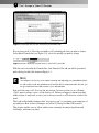
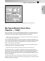
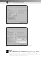
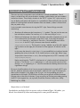
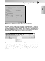
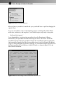
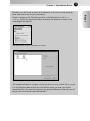
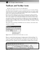
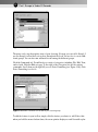
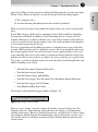
AL
Chapter 1
TE
RI
Spreadsheet Basics
MA
In This Chapter
D
◆ Learning things about spreadsheets you don’t typically find in manuals and
classes
◆ Fixing up odd behavior in your spreadsheets
TE
◆ Setting Excel macro security
GH
◆ Getting the most out of an Excel menu
◆ Understanding Excel templates
RI
◆ Taming your Excel toolbars
PY
◆ Alleviating window “pains” in Excel
CO
A Good Place to Begin
Have you ever wanted to individually format different words in a sentence or
phrase appearing in a spreadsheet, such as those appearing in Figure 1-1? If
you haven’t thought about or attempted to do so, put the book down and try it
now. It’s a simple enough task, but it’s not so obvious if you haven’t done it
before.
3
4
Part I: Escape in Under 30 Seconds
Figure 1-1: Spreadsheet cells with individually formatted words
Here is how you do it. Select the spreadsheet cell containing the text you want to format.
In the Excel Formula Bar (see Figure 1-2), select the word(s) you want to change.
Figure 1-2: Edit individually selected words in the Excel Formula Bar.
With the text selected in the Formula Bar, click Format➪Cells and you will be presented
with a dialog box like that shown in Figure 1-3.
NOTE
I should point out that if you are used to entering and adjusting your spreadsheet formulas and content inside the spreadsheet cell and are able to select text within the cell, you
can go ahead and format the content of your selected text.
Now, isn’t this easy to do? It is easy but not obvious, because you have to use a Format
“Cells” menu to change a piece of text inside a cell. Unless you happen to know about this
hidden feature, it may never occur to you to that you can use a cell feature for a subcell element!
This book is filled with techniques that “may never occur” to you during your normal use of
spreadsheets. Most of these techniques are in Part I (“Escape in Under 30 Seconds”).
This chapter and the ones to follow outline some commonly encountered problems and
challenges, and some easy fixes.
Chapter 1: Spreadsheet Basics
5
Part I
Figure 1-3: Format the selected word as you would regularly format a spreadsheet cell.
My Spreadsheets Have Gone
Haywire — Help!!
Every now and then, it looks as though something with Excel is totally messed up. These
“haywire” moments are typically caused by Excel having the wrong settings. In this section, I outline a few issues relating to settings and show some easy fixes.
“When I enter the value 12, Excel turns it into 0.12, but when I enter 12.24, Excel keeps it the way I entered
it. How can I prevent this from happening?”
The very first time this problem is encountered, it must be bewildering. Fortunately, it is
easy to fix. Choose Tools➪Options and click the Edit tab. You will notice that Excel allows
you to set fixed decimals. If there is a checkmark next to this setting, uncheck it (see
Figure 1-4) and then click the OK button.
In some cases, it may be easier to enter a long list of numbers using fixed decimals, but
generally this causes more confusion than it avoids.
“My spreadsheet columns are labeled using numbers instead of letters. I want to change it back.”
Sometimes you’ll be given a spreadsheet in which the columns appear with numbers
instead of letters. This is referred to as the “R1C1” style. The usual display of column letters is known as the “A1” style. Excel supports both ways of displaying spreadsheets.
That’s because the underlying formulas and values used by Excel have nothing to do with
how they are displayed.
To change your setting, choose Tools➪Options and click the General tab. You will notice
that Excel allows you to set R1C1. Uncheck this setting (see Figure 1-5) and then click the
OK button to get back the A1 style.
6
Part I: Escape in Under 30 Seconds
Figure 1-4: Disable (uncheck) the “Fixed decimal” setting.
Figure 1-5: Uncheck the “R1C1 reference style” to get back the A1 style.
NOTE
There is a spreadsheet on your CD-ROM called ch01_02SwitchTool.xls. When you
open this spreadsheet you will see two buttons labeled R1C1 and A1. Clicking the
appropriate button will allow you to switch back and forth between the two reference
styles without having to go through the Excel menus.
Chapter 1: Spreadsheet Basics
7
Understanding the R1C1 reference style
I want to explain some features of using the R1C1 style. Several things are worth
mentioning.
• Absolute cell references don’t require any “$” symbols. They are just the row number and column number. For instance, $D$10 is the same thing as R10C4.
• Relative cell references are shown with brackets around the respective row or column number offset. For example, using the A1 style, if you copy the formula
=K2+U2+AE2 from cell A2 and paste it into cell D7, the resulting formula will be
=N7+X7+AH7. In the R1C1 style, the exact same formula would be
=RC[10]+RC[20]+RC[30]. The formula is saying, “add the sum of the cells appearing 10 columns to the right plus 20 columns to the right plus 30 columns to the
right.”
In this sense the formula is visual, that is, it is not too difficult to visualize a formula
grabbing the values of the cells 10, 20, and 30 columns to the right. When I copy
and paste this formula from A2 to D7, the resulting formula (in R1C1 notation) is still
=RC[10]+RC[20]+RC[30].
Notice one thing else: The R1C1 style formula isn’t tied to which cell the formula is
written in. The formula =$A2+B3 appearing in D6 will not match the results of the
formula =$A2+B3 appearing in G17. You have two identical-looking formulas meaning different things!
By now it should be obvious that I have a personal preference for using the R1C1 style
over A1. However, because most of the world is used to the A1 style, I have kept just
about all the examples in this book in the A1 style. I am also providing you with a
spreadsheet on the book’s CD-ROM that will allow you to go back and forth between
the two styles at the click of a button. If you are curious to find out more about putting
the R1C1 style to good use, see my book, Excel Best Practices for Business (Wiley
Publishing, Inc., 2004).
“My spreadsheets are all backward!”
Spreadsheets can display labels in reverse order as shown in Figure 1-6 (and no, you
haven’t been abducted by aliens and transported to some parallel universe).
Part I
There are two ways to represent rows and columns in Excel spreadsheets. One of
these is to label them with row and column numbers, and the other uses row numbers
and column letters. These labels, whether in the “R1C1” style or “A1” style, are just a
way to display and specify cell locations on a spreadsheet. Because Excel gives you the
option of switching back and forth between these two modes, it doesn’t matter which
one you prefer using.
8
Part I: Escape in Under 30 Seconds
Figure 1-6: This spreadsheet is reversed (column labels all go in the wrong order and rows appear
on the right instead of the left side).
So, how does this situation come about and why would Excel allow you to do this? It’s very
simple (see Figure 1-7). Excel is used in many countries and many languages. In some languages, the order of text flows from right to left, in contrast to English. If the natural orientation for a language is from right to left, wouldn’t it be more natural if you could start
the column and row labels from the top-right corner? Excel allows you to make this kind of
customization. From the Excel menu, click Tool➪Options and click the International tab,
as shown in Figure 1-7.
To return the orientation to the usual left to right, uncheck the View Current Sheet Rightto-left setting. Also make sure that the Default direction is set Left-to-right (refer to
Figure 1-7).
So, how might these settings all get changed? I’ll give you one way. One member in my
family tends to click any button without realizing what he’s changing. My mother affectionately refers to him as “having pepper in his fingers.” Maybe there is someone in your family
with pepper in his fingers!
I am willing to bet that some of you who try to navigate to the Excel Options window are
stumped by another problem: Excel won’t allow you to go to the Tools menu and select
Options. It’s grayed out!
Chapter 1: Spreadsheet Basics
9
Part I
Figure 1-7: You can adjust settings to go from right to left or from left to right.
Excel allows you to set options that tell the software how it should behave at any time. To
be able to set your options (such as the International setting), you need to have a spreadsheet already open. It doesn’t matter which one, and the settings you choose don’t apply to
any specific spreadsheet. If you try to get to the Options menu item while no spreadsheets
are open, you will see the Options menu item grayed out (see Figure 1-8).
Figure 1-8: The Options item on the Excel Tools menu is grayed out when no spreadsheet is open.
To fix this situation, simply make sure that a spreadsheet file is open first. It doesn’t matter which spreadsheet file is open. If you haven’t created any or can’t find a spreadsheet,
simply click New from the Excel File menu (or press Ctrl+N). If Excel doesn’t create a file
but displays a bunch of possible files on a panel on the right (see Figure 1-9), select Blank
Workbook.
10
Part I: Escape in Under 30 Seconds
Figure 1-9: Options for New Workbook
After you have a spreadsheet or workbook open, you should have no problem changing the
options. Try it.
If you are new to Excel, some of the terminology may be confusing. The sidebar “Excel
workbooks, worksheets, and templates,” later in this chapter, may clarify a few points.
“My Formula Bar disappeared.”
I once downloaded a very interesting spreadsheet from the Department of Energy.
Unfortunately, the spreadsheet had an interesting side effect. The macros used in the
spreadsheet tried to make the spreadsheet behave like a traditional software application
and removed the Formula Bar. After the spreadsheet was closed, the Formula Bar did not
reappear. Though this kind of problem is annoying, it’s solved with another quick fix. From
the Excel menu, click Tools➪Options, click the View tab, as shown in Figure 1-10, and
then click the OK button.
Figure 1-10: Check the setting for the Formula Bar in the View tab.
Chapter 1: Spreadsheet Basics
11
Macro Security
Figure 1-11 shows the kind of warning error you will get if you open a spreadsheet containing a macro and your security settings in Excel are set to High.
Figure 1-11: Warning message presented by Excel that tells you it disabled the
spreadsheet macros
NOTE
Unlike the rest of Excel, which contains numbers and calculation formulas, macros contain programming code. Macros can extend the capability of a spreadsheet to do more
than straight computations. They can add interactivity and intelligence in a way that formulas by themselves cannot. This capability is good, but it also presents some dangers.
For this reason, Microsoft sets the security settings for Excel macros to High, thereby
disabling macros unless they come from a trusted source.
Unless the spreadsheet containing a macro has been digitally signed and that signature
can be verified, you will be unable to run the macros as long as your security settings are
set to High or Very High. Incidentally, when Excel is first installed on your computer, the
default setting is High. This means that if you never touched your security settings, you
would not be able to run any Excel spreadsheet containing macros unless it was digitally
signed and specifically trusted by you.
Although this is surely the safest way of configuring your software at the time of your
install, having a high security setting can get in the way if you are frequently receiving
spreadsheets with macros from people you trust but the spreadsheets lack the needed digital signatures. Even then, you have no guarantee that the macros will be safe. All you are
doing is saying that you trust the source that is providing you with the spreadsheet, and
you trust that it hasn’t been altered in some way by a potentially malicious third party.
Let me give you the quick and practical solution. Set your security setting to Medium. You
can do this by clicking Tools➪Macro➪Security and, in the Security Level tab, click the button next to Medium (see Figure 1-12).
Part I
“Excel won’t let me run any spreadsheets that have macros. What can I do?”
12
Part I: Escape in Under 30 Seconds
Figure 1-12: Adjusting your Security Level setting to Medium
Here is what this accomplishes. Anytime you open a spreadsheet that contains macro code,
Excel will ask whether you want to enable or disable macros. This setting gives you maximum flexibility. Instead of unilaterally disabling macros, it allows you to decide whether to
enable the macros at the time you open the spreadsheet file.
CAUTION
Disabling the macros doesn’t mean that the macros are disabled for all time. They are
just disabled at the time you happen to open the spreadsheet file. If you close the file
and e-mail it to a friend, the file will still contain the macros. Unless your friend also does
something to disable the macros, the macros will be enabled.
If you want to play it safe, just select Disable Macros with the Medium Security Level settings. Later in the book (see Chapters 4 and 10), I show you how to inspect the macros for
yourself. If you plan on working with spreadsheets you trust but that have macros, then
setting your macro Security Level to Medium is recommended.
Excel Menus
“Excel never shows a full menu unless I click the double arrow at the bottom of the menu or wait a few seconds for the menu to expand. If I select an item on the expanded list, it then gets added to the short list. As a
result, my menus are constantly changing in appearance! How can I once and for all get the menus to be fully
expanded and unchanging?”
The accordion pull-down menu system (see Figure 1-13) used in Excel is a classic overengineered solution that many people find annoying but don’t know how to fix.
Chapter 1: Spreadsheet Basics
13
Part I
Figure 1-13: Abbreviated menu with double arrow
Here’s how to fix it:
1. Click the Customize feature from the Tools menu.
The Customize window with its three tabs appears.
2. Click the tab labeled Options.
3. The second checkbox, Always Show Full Menus, is not selected. Click this checkbox to
make sure that full menus are enabled.
4. Click the Close button to accept the changes you made.
Excel workbooks, worksheets, and templates
While we’re at it, let’s get the terminology straight. When a spreadsheet file in Excel is
being opened or referred to, it is called a workbook. Within each workbook you will
see tabs appearing along the bottom. These tabs may have generic names such as
Sheet1 or Sheet2. When you click any of these tabs, a sheet appears that corresponds
to the tab name. Not surprisingly, these sheets are referred to as worksheets.
When you open a new workbook (do so by clicking File➪New from the Excel menu),
you typically see multiple worksheets, which are named Sheet1, Sheet2, and so forth.
The individual worksheets are all empty initially; when you move between worksheets,
you see no differences between them. After you start populating them with data or
formulas, you will easily know which worksheet you are looking at. You have several
ways to move between worksheets. You can click the tab appearing at the bottom of
the worksheet. Or press Ctrl+PgDn or Ctrl+PgUp. Notice that to the bottom left of the
worksheet, tabs appear as a bunch of triangular arrows. These help you to navigate
through the list of worksheets.
From time to time you may hear about Excel templates. An Excel template is not a
generic term but is actually a specific type of spreadsheet file that you can create and
use. The filename suffix for a template file is .xlt instead of the usual .xls.
continued
14
Part I: Escape in Under 30 Seconds
continued
Excel templates are well suited for finely tuned spreadsheets that you will use
repeatedly. A good example is a time sheet that could be distributed to a group of
people. Perhaps, instead of using a template, you could commandeer an already
populated spreadsheet and clean out the data. Would this be a good idea? What if
you accidentally miss clearing out all the data or inadvertently clobber a spreadsheet
formula? These are reasons that you may want to think about using template files.
Creating a template is easy. When you save your spreadsheet, click File➪Save As (see
the following figure).
Saving a file as an .XLT template
Keep in mind that the .xlt file is typically stored in the Documents and Setting
directory, usually inside the Application Data\Microsoft\Templates directory of your
Application Data folder (see the next figure).
Typical location of Excel Templates
Chapter 1: Spreadsheet Basics
15
Thankfully, you don’t have to search for the directory in which to save the templates.
Excel takes care of that for you automatically.
Standard location of Excel Templates you create
Templates located in the General tab
Your template will open as a regular .xls file, but when you save it, Excel will try to save
it in the Templates folder and not the usual location where you keep your regular
spreadsheet files. You need to navigate to your preferred directory; otherwise, you will
end up with a lot of clutter and misplaced files!
Part I
To open a template, click File➪New and then, in the Templates list, click On my
computer (see the first figure that follows) and select the template (as shown in the
second figure that follows).
16
Part I: Escape in Under 30 Seconds
Toolbars and Toolbar Icons
“My toolbar is missing some icons that it used to have! What happened?”
Just underneath your Excel menu is a series of icons placed on a set of toolbars. Clicking
each of these icons causes Excel to perform a particular task. There are benefits of using
toolbar icons: They are very accessible (except when hidden!) and are often quicker than
trying to do the equivalent through the Excel menu.
Here is the problem and what you can do about it. If you have more toolbar icons than
there is space across your Excel application window to hold them, Excel will try to park
these icons somewhere. Out of the box, Excel will hide some of them, but it doesn’t do a
very good job of letting you know that there are hidden icons. It gives a visual signal, but
it’s subtle: Look for a couple of extra “notches” on the right side of the toolbar. When you
click these notches, the hidden toolbars become visible (see Figure 1-14) and you can click
the icon you want.
This method works, but having to find hidden icons sort of defeats a chief benefit—their
immediate accessibility.
Figure 1-14: Click the toolbar notch to make hidden icons visible.
There is a second solution, but it may not be what you want. Look back at Figure 1-14.
You’ll notice an option called Show Buttons on Two Rows. If you select this option, your
toolbar icons will be visible, but they will occupy multiple rows (see Figure 1-15). If you
don’t happen to have a gigantic screen, you’ll pay dearly for valuable screen real estate.
Figure 1-15: Toolbar icons are visible but there is a lot of wasted space.
Chapter 1: Spreadsheet Basics
17
“A toolbar that I don’t need is on my screen. How do I make it go away?”
The answer is easy if your toolbar happens to be free floating. Simply click the X at the
top-right of your toolbar. However, toolbars that are nestled directly under the Excel menu
do not have that X. For these, click Tools➪Customize and click the Toolbars tab. You will
see a list of toolbars. The ones that are visible have a checkmark next to them. Uncheck
the ones you no longer wish to see. If you want to experiment with some of the toolbars
that are not visible, simply place a checkmark next to their names and they’ll be instantly
visible.
Customizing Your Excel Software with
Toolbars
At this point I would like you to define some custom toolbars of your own. Ultimately, the
ones you choose are up to you. Just keep in mind that you’ll quickly run out of screen
space if you activate too many toolbars. I show you some useful ones you may want to keep
as part of your standard arsenal.
If you have never customized your toolbars, they may appear similar to those in
Figure 1-16.
Figure 1-16: Excel default settings
You can add to the existing slate of toolbars on your screen, but I would like you to construct your own custom group. First, go to the Excel menu and click Customize. Notice the
three tabs running across the top of your Customize window. Make sure that the Toolbars
tab is the frontmost tab showing. If it’s not, click it. When you see the checklist of predefined toolbars, click the New button to create your own custom toolbar (see Figure 1-17).
Part I
A third solution is available. It entails customizing your toolbars to contain only the icons
you need. This is likely to be your best approach, but it involves more than a 30-second
point-and-click escape. The next section, “Customizing Your Excel Software with Toolbars,”
outlines the steps.
18
Part I: Escape in Under 30 Seconds
Figure 1-17: Give your custom toolbar a name.
The name can be any descriptive name of your choosing. For now, you can call it Group1. I
use the Group1 toolbar that’s set up here throughout the book. You are free to create additional groups. You can also mix and match icons among the different groups.
Click the Commands tab. You will notice a variety of categories, including File, Edit, View,
and so forth. Click the Edit category. To the right of the Categories list are the various
commands. Scroll down on the right till you see Paste Formatting (see Figure 1-18). Click
Paste Formatting to select it.
Figure 1-18: Select a toolbar icon to add to your custom group.
To add the feature to your toolbar, simply click the feature you desire to add. Notice that
when you hold the mouse button down, the arrow pointer displays a small box with a plus
Chapter 1: Spreadsheet Basics
19
sign (+) in it. While you have your mouse button held down, drag the icon onto your empty
Group1 toolbar. When you drag the icon onto the Group1 toolbar, two things happen:
2. A vertical insertion point indicates where the icon will be positioned.
When you release the mouse button inside the Group1 toolbar, you see the icon deposited
there.
For the Edit Category, add the toolbar commands for Paste Values and Clear Formatting.
You may have noticed that in addition to Clear Formatting, there is a feature for Clear
Contents. Although you could also add this icon to your toolbar, it won’t really benefit you
to do so, because you can clear the contents of any cells on the spreadsheet that happen to
be selected just by pressing the Del key.
Feel free to experiment and try adding any variety of command icons to your toolbar that
you want. Whatever helps you to be productive is great. Also keep in mind that unless you
have a super-gigantic screen, the real estate space on your computer display can be a precious commodity. After you’ve had a chance to experiment with the different toolbar icons,
pick the ones that are most useful to you (that is, the ones you will use on a regular basis).
To get off to a good start and have in place the icons that will be used throughout the book,
add the following to your toolbar:
•
From the View category: Zoom In and Zoom Out
•
From the Insert category: Diagram
•
From the Format category: Light Shading
•
From the Tools category: Trace Precedents, Trace Dependents, Remove All Arrows
•
From the Data category: Text To Columns
•
From Window and Help Freeze Panes
Your Group1 toolbar should now appear similar to Figure 1-19.
Figure 1-19: Group1 custom toolbar
There are “space saving” icons that combine the benefits of several toolbar icons. The
Diagram icon is one. Icons and menu options that have the ellipsis (...) following them
often have this feature. When you click the Diagram icon, you will be able to choose among
Cycle diagrams, Radial diagrams, Pyramid diagrams, and so forth. Unless you have a specific favorite and use it constantly, you won’t really need all the different options in your
custom toolbar.
Part I
1. The + changes to an x.
20
Part I: Escape in Under 30 Seconds
Sometimes you will want specific toolbar icons even though you can access the feature
through one of the space-saving icons. The Paste Values and Paste Formatting are such
icons. Being able to paste pure values that are devoid of formulas and formatting information is an important feature to have. Likewise, being able to paste formats will facilitate
your ability to manage spreadsheet information.
Some of you who are already used to using the Format Painter may be wondering, “Why
bother at all with the Paste Formatting when I have the Format Painter?” The Format
Painter just clones the format of a selected region of cells at a new location. If, in addition
to formatting, you also want to paste the values, then you’ll need to do more than just use
the Format Painter. You’ll have to go back to your original selection of cells and then copy
and paste the values. This adds to the number of steps you need to perform and will slow
you down. If you feel tightly wedded to the Format Painter, do not fret. Continue using
what you’re already adept at. Old habits die hard. Some of them are important to keep.
Others should be shed. Ultimately, you’re the best person to make that call.
Keep in mind that all of the facilities of these toolbars are generally accessible through the
Excel menus.
The Freeze Pane is particularly practical. I can’t tell you how often I see spreadsheets in a
split mode, as in Figure 1-20. Sometimes I think the split-pane feature of spreadsheets
should really be called the “Split Pain” feature. This problem is easily corrected if you use
the Freeze Pane icon (see Figure 1-21). The Freeze Pane icon acts as a toggle switch,
enabling you to quickly switch back and forth. You can find the Freeze/Unfreeze Pane feature in the Excel Window menu, but using the toolbar icon is much quicker.
Figure 1-20: Confusing use of split-pane
Chapter 1: Spreadsheet Basics
21
Part I
Figure 1-21: After you click the Freeze Pane icon, the confusing split-pane is gone and the
spreadsheet scrolls naturally with a split screen.
Text to Column is a feature that is particularly handy if you’re going to be working with
data files that are provided from third-party sources, such as government-published information pulled off the Internet.
Here’s the last bit of configuration and I’ll be done with toolbars. Right now, your Group1
toolbar (refer to Figure 1-19) is floating somewhere on your screen, because I haven’t told
you to anchor it to the standard Excel toolbars. Just click the Group1 toolbar anywhere on
the title bar and the mouse point will take on a compass-like appearance. Holding the
mouse button down, drag the toolbar over to the other toolbars and the Group1 toolbar will
snap into place (see Figure 1-22).
Figure 1-22: Three rows of toolbars
Be careful not to unintentionally park the toolbar above the menu or over to one of the
edges of your Excel application window. If a toolbar does get too close to the top, bottom,
left, or right, it will snap to that edge. To unglue the toolbar from the edge, place your
mouse over the top-left corner of the toolbar (there should be series of textured vertical
dots), click your mouse to grab the toolbar, and move it away.
Notice that the toolbars take up three rows and there’s a fair amount of empty space.
Unless you’re using a really large screen, you may want to consolidate all the toolbars into
22
Part I: Escape in Under 30 Seconds
two rows. They can be shoved onto the second row, but there is not quite enough space to
simultaneously display all of them on a straight horizontal line.
I don’t know about you, but I don’t particularly like the idea of using second-class icons. If
they’re out of sight, they’re out of mind. Also, what’s the purpose of having hidden icons
when you already have their underlying capabilities in the Excel menus?
My first way of fixing this is to effectively remove the icons I don’t expect to be using.
There are a number of strategies. You can keep the Group1 toolbar at its full length and try
resizing the formatting toolbar on its left to be a shorter width. This will relegate some of
the Formatting icons to second class. Somehow this is not so palatable.
You could whisk away some of the icons to never-never land, dragging and dropping them
to the desktop area. By doing so, you would be modifying an Excel standard feature, which
I’m not sure you would want to do.
There’s another way that’s quite safe. Construct a new toolbar called Formatting2 (or
whatever name you want to give it). Add to this toolbar the formatting facilities you need
and exclude the rest. In the Customize Options menu, deselect the Formatting toolbar and
check the newly created Formatting2 toolbar. Now there are no second-class icons and they
all fit on two rows.
Nothing forces you to keep toolbars at the top of the spreadsheet. Aside from having them
hover somewhere around, you can park them off to the side.
Closing Thoughts
This chapter’s main purpose is to get out of the way those annoying particulars that routinely hamper spreadsheet productivity. With luck, most of you haven’t come across a significant number of problems like the kind outlined here. If you do, you will find some easy
fixes here. Also, you can find additional material at
http://www.EscapeFromExcelHell.com.