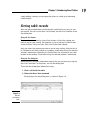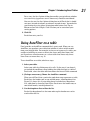
1
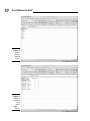
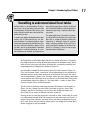
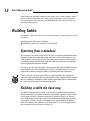
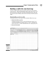
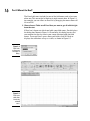
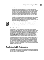
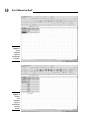
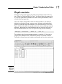
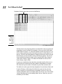
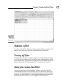
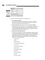
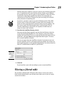
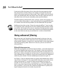
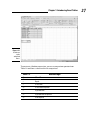
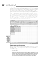
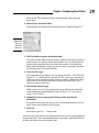
Chapter 1
AL
Introducing Excel Tables
In This Chapter
RI
Figuring out tables
Building tables
TE
Analyzing tables with simple statistics
Sorting tables
MA
Discovering the difference between using AutoFilter and filtering
D
F
RI
GH
TE
irst things first. I need to start my discussion of using Excel for data
analysis by introducing Excel tables, or what Excel used to call lists.
Why? Because, except in the simplest of situations, when you want to analyze
data with Excel, you want that data stored in a table. In this chapter, I discuss
what defines an Excel table; how to build, analyze, and sort a table; and why
using filters to create a subtable is useful.
PY
What Is a Table and Why Do I Care?
CO
A table is, well, a list. This definition sounds simplistic, I guess. But take a
look at the simple table shown in Figure 1-1. This table shows the items that
you might shop for at a grocery store on the way home from work.
As I mention in the introduction of this book, many of the Excel workbooks
that you see in the figures of this book are available in a compressed Zip file
available at the Dummies Web site. You can download this Zip file from www.
dummies.com/go/e2007dafd.
Commonly, tables include more information than Figure 1-1 shows. For example, take a look at the table shown in Figure 1-2. In column A, for example, the
table names the store where you might purchase the item. In column C, this
expanded table gives the quantity of some item that you need. In column D,
this table provides a rough estimate of the price.
10
Part I: Where’s the Beef?
Figure 1-1:
A table:
Start out
with the
basics.
Figure 1-2:
A grocery
list for the
more
serious
shopper . . .
like me.
Chapter 1: Introducing Excel Tables
Something to understand about Excel tables
An Excel table is a flat-file database. That flatfile-ish-ness means that there’s only one table
in the database. And the flat-file-ish-ness also
means that each record stores every bit of information about an item.
In comparison, popular desktop database applications such as Microsoft Access are relational databases. A relational database stores
information more efficiently. And the most striking way in which this efficiency appears is that
you don’t see lots of duplicated or redundant
information in a relational database. In a relational database, for example, you might not see
Sams Grocery appearing in cells A2, A3, A4, and
A5. A relational database might eliminate this
redundancy by having a separate table of grocery stores.
This point might seem a bit esoteric; however,
you might find it handy when you want to grab
data from a relational database (where the
information is efficiently stored in separate
tables) and then combine all this data into a
super-sized flat-file database in the form of an
Excel list. In Chapter 2, I discuss how to grab
data from external databases.
An Excel table usually looks more like the list shown in Figure 1-2. Typically,
the table enumerates rather detailed descriptions of numerous items. But a
table in Excel, after you strip away all the details, essentially resembles the
expanded grocery-shopping list shown in Figure 1-2.
Let me make a handful of observations about the table shown in Figure 1-2.
First, each column shows a particular sort of information. In the parlance of
database design, each column represents a field. Each field stores the same
sort of information. Column A, for example, shows the store where some item
can be purchased. (You might also say that this is the Store field.) Each piece
of information shown in column A — the Store field — names a store: Sams
Grocery, Hughes Dairy, and Butchermans.
The first row in the Excel worksheet provides field names. For example, in
Figure 1-2, row 1 names the four fields that make up the list: Store, Item,
Quantity, and Price. You always use the first row, called the header row,
of an Excel list to name, or identify, the fields in the list.
Starting in row 2, each row represents a record, or item, in the table. A record
is a collection of related fields. For example, the record in row 2 in Figure 1-2
shows that at Sams Grocery, you plan to buy two loaves of bread for a price
of $1 each. (Bear with me if these sample prices are wildly off; I usually don’t
do the shopping in my household.)
11
12
Part I: Where’s the Beef?
Row 3 shows or describes another item, coffee, also at Sams Grocery, for $8.
In the same way, the other rows of the super-sized grocery list show items
that you will buy. For each item, the table identifies the store, the item, the
quantity, and the price.
Building Tables
You build a table that you want to later analyze by using Excel in one of
two ways:
Export the table from a database.
Manually enter items into an Excel workbook.
Exporting from a database
The usual way to create a table to use in Excel is to export information from a
database. Exporting information from a database isn’t tricky. However, you
need to reflect a bit on the fact that the information stored in your database
is probably organized into many separate tables that need to be combined
into a large flat-file database or table.
In Chapter 2, I describe the process of exporting data from the database and
then importing this data into Excel so it can be analyzed. Hop over to that
chapter for more on creating a table by exporting and then importing.
Even if you plan to create your tables by exporting data from a database,
however, read on through the next paragraphs of this chapter. Understanding
the nuts and bolts of building a table makes exporting database information
to a table and later using that information easier.
Building a table the hard way
The other common way to create an Excel table (besides exporting from a
relational database) is to do it manually. For example, you can create a table
in the same way that I create the grocery list shown in Figure 1-2. You first
enter field names into the first row of the worksheet and then enter individual records, or items, into the subsequent rows of the worksheet. When a
table isn’t too big, this method is very workable. This is the way, obviously,
that I created the table shown in Figure 1-2.
Chapter 1: Introducing Excel Tables
Building a table the semi-hard way
To create a table manually, what you typically want to do is enter the field
names into row 1, select those field names and the empty cells of row 2, and
then choose Insert➪Table. Why? The Table command tells Excel, right from
the get-go, that you’re building a table. But let me show you how this process
works.
Manually adding records into a table
To manually create a list by using the Table command, follow these steps:
1. Identify the fields in your list.
To identify the fields in your list, enter the field names into row 1 in a
blank Excel workbook. For example, Figure 1-3 shows a workbook fragment. Cells A1, B1, C1, and D1 hold field names for a simple grocery list.
2. Select the Excel table.
Figure 1-3:
The start of
something
important.
13
14
Part I: Where’s the Beef?
The Excel table must include the row of the field names and at least one
other row. This row might be blank or it might contain data. In Figure 1-3,
for example, you can select an Excel list by dragging the mouse from cell
A1 to cell D2.
3. Choose Insert➪Table to tell Excel that you want to get all official right
from the start.
If Excel can’t figure out which row holds your field names, Excel displays
the dialog box shown in Figure 1-4. Essentially, this dialog box just lets
you confirm that the first row in your range selection holds the field
names. To accept Excel’s guess about your table, click OK. Excel redisplays the worksheet set up as a table, as shown in Figure 1-5.
Figure 1-4:
Excel tries
to figure out
what you’re
doing.
Figure 1-5:
Enter your
table rows
into nicely
colored
rows.
Chapter 1: Introducing Excel Tables
4. Describe each record.
To enter a new record into your table, fill in the next empty row. For
example, use the Store text box to identify the store where you purchase
each item. Use the — oh, wait a minute here. You don’t need me to tell
you that the store name goes into the Store column, do you? You can
figure that out. Likewise, you already know what bits of information go
into the Item, Quantity, and Price column, too, don’t you? Okay. Sorry.
5. Store your record in the table.
Click the Tab or Enter button when you finish describing some record or
item that goes onto the shopping list. Excel adds another row to the
table so that you can add another item. Excel shows you which rows and
columns are part of the table by using color.
Previous versions of Excel included a Data➪Form command, which was
another way to enter records into an Excel table. When you chose the
Data➪Form command, Excel displayed a cute, little, largely useless
dialog box that collected the bits of record information and then entered
them into the table.
Some table-building tools
Excel includes an AutoFill feature, which is particularly relevant for table
building. Here’s how AutoFill works: Enter a label into a cell in a column where
it’s already been entered before, and Excel guesses that you’re entering the
same thing again. For example, if you enter the label Sams Grocery in cell A2
and then begin to type Sams Grocery in cell A3, Excel guesses that you’re
entering Sams Grocery again and finishes typing the label for you. All you
need to do to accept Excel’s guess is press Enter. Check it out in Figure 1-6.
Excel also provides a Fill command that you can use to fill a range of cells —
including the contents of a column in an Excel table — with a label or value.
To fill a range of cells with the value that you’ve already entered in another
cell, you drag the Fill Handle down the column. The Fill Handle is the small
plus sign (+) that appears when you place the mouse cursor over the lowerright corner of the active cell. In Figure 1-7, I use the Fill Handle to enter Sams
Grocery into the range A5:A12.
Analyzing Table Information
Excel provides several handy, easy-to-use tools for analyzing the information
that you store in a table. Some of these tools are so easy and straightforward
that they provide a good starting point.
15
16
Part I: Where’s the Beef?
Figure 1-6:
A little
workbook
fragment,
compliments
of AutoFill.
Figure 1-7:
Another
little
workbook
fragment,
compliments
of the Fill
Handle.
Chapter 1: Introducing Excel Tables
Simple statistics
Look again at the simple grocery list table that I mention earlier in the section, “What Is a Table and Why Do I Care?” See Figure 1-8 for this grocery list
as I use this information to demonstrate some of the quick-and-dirty statistical tools that Excel provides.
One of the slickest and quickest tools that Excel provides is the ability to
effortlessly calculate the sum, average, count, minimum, and maximum of
values in a selected range. For example, if you select the range C2 to C10 in
Figure 1-8, Excel calculates an average, counts the values, and even sums the
quantities, displaying this useful information in the status bar. In Figure 1-8,
note the information on the status bar (the lower edge of the workbook):
Average: 1.555555556
Count: 9
Sum: 14
This indicates that the average order quantity is (roughly) 1.5, that you’re
shopping for 9 different items, and that the grocery list includes 14 items:
Two loaves of bread, one can of coffee, one tomato, one box of tea, and so on.
Figure 1-8:
Start at the
beginning.
17
18
Part I: Where’s the Beef?
The big question here, of course, is whether, with 9 different products but a
total count of 14 items, you’ll be able to go through the express checkout line.
But that information is irrelevant to our discussion. (You, however, might want
to acquire another book I’m planning, Grocery Shopping For Dummies.)
You aren’t limited, however, to simply calculating averages, counting
entries, and summing values in your list. You can also calculate other
statistical measures.
To perform some other statistical calculation of the selected range list,
right-click the status bar. When you do, Excel displays a pop-up Status Bar
Configuration menu. Near the bottom of that menu bar, Excel provides six statistical measures that you can add to or remove from the Status Bar: Average,
Count, Count Numerical, Maximum, Minimum, and Sum. In Table 1-1, I
describe each of these statistical measures briefly, but you can probably
guess what they do. Note that if a statistical measure is displayed on the
Status Bar, Excel places a check mark in front of the measure on the Status Bar
Confirmation menu. To remove the statistical measure, select the measure.
Table 1-1
Quick Statistical Measures Available on the Status Bar
Option
What It Does
Count
Tallies the cells that hold labels, values, or formulas. In other
words, use this statistical measure when you want to count
the number of cells that are not empty.
Count Numerical
Tallies the number of cells in a selected range that hold
values or formulas.
Maximum
Finds the largest value in the selected range.
Minimum
Finds the smallest value in the selected range.
Sum
Adds up the values in the selected range.
No kidding, these simple statistical measures are often all you need to gain
wonderful insights into data that you collect and store in an Excel table. By
using the example of a simple, artificial grocery list, the power of these quick
statistical measures doesn’t seem all that earthshaking. But with real data,
these measures often produce wonderful insights.
In my own work as a writer, for example, I first noticed the slowdown in the
computer book publishing industry that followed the dot.com meltdown
when the total number of books that one of the larger distributors sold —
information that appeared in an Excel table — began dropping. Sometimes,
Chapter 1: Introducing Excel Tables
simply adding, counting, or averaging the values in a table gives extremely
useful insights.
Sorting table records
After you place information in an Excel table, you’ll find it very easy to sort
the records. You can use the Sort A to Z button, the Sort Z to A button, or the
Sort dialog box.
Using the Sort buttons
To sort table information by using a Sort buttons, click in the column you
want to use for your sorting. For example, to sort a grocery list like the one
shown in Figure 1-8 by the store, click a cell in the Store column.
After you select the column you want to use for your sorting, click the Sort A
to Z button to sort table records in ascending, A-to-Z order using the selected
column’s information. Alternatively, click the Sort Z to A button to sort table
records in descending, Z-to-A order using the selected column’s information.
Using the Sort dialog box
When you can’t sort table information exactly the way you want by using the
Sort A to Z and Sort Z to A buttons, use the Sort dialog box.
To use the Sort dialog box, follow these steps:
1. Click a cell inside the table.
2. Choose the Data➪Sort command.
Excel displays the Sort dialog box, as shown in Figure 1-9.
Figure 1-9:
Set sort
parameters
here.
19
20
Part I: Where’s the Beef?
3. Select the first sort key.
Use the Sort By drop-down list to select the field that you want to use for
sorting. Next, choose what you want to use for sorting: values, cell
colors, font colors, or icons. Probably, you’re going to sort by values, in
which case, you’ll also need to indicate whether you want records
arranged in ascending or descending order by selecting either the
ascending A to Z or descending Z to A entry from the Order box.
Ascending order, predictably, alphabetizes labels and arranges values in
smallest-value-to-largest-value order. Descending order arranges labels
in reverse alphabetical order and values in largest-value-to-smallestvalue order. If you sort by color or icons, you need to tell Excel how it
should sort the colors by using the options that the Order box provides.
Typically, you want the key to work in ascending or descending order.
However, you might want to sort records by using a chronological
sequence, such as Sunday, Monday, Tuesday, and so on, or January,
February, March, and so forth. To use one of these other sorting options,
select the custom list option from the Order box and then choose one of
these other ordering methods from the dialog box that Excel displays.
4. (Optional) Specify any secondary keys.
If you want to sort records that have the same primary key with a secondary key, click the Add Level button and then use the next row of
choices from the Then By drop-down lists to specify which secondary
keys you want to use. If you add a level that you later decide you don’t
want or need, click the sort level and then click the Delete Level button.
You can also duplicate the selected level by clicking Copy Level. Finally,
if you do create multiple sorting keys, you can move the selected sort
level up or down in significance by clicking the Move Up or Move Down
buttons.
Note: The Sort dialog box also provides a My Data Has Headers check
box that enables you to indicate whether the worksheet range selection
includes the row and field names. If you’ve already told Excel that a
worksheet range is a table, however, this check box is disabled.
5. (Really optional) Fiddle-faddle with the sorting rules.
If you click the Options button in the Sort dialog box, Excel displays the
Sort Options dialog box, shown in Figure 1-10. Make choices here to further specify how the first key sort order works.
Figure 1-10:
Sorting out
your sorting
options.
Chapter 1: Introducing Excel Tables
For a start, the Sort Options dialog box enables you to indicate whether
case sensitivity (uppercase versus lowercase) should be considered.
You can also use the Sort Options dialog box to tell Excel that it should
sort rows instead of columns or columns instead of rows. You make this
specification by using either Orientation radio button: Sort Top to
Bottom or Sort Left to Right. Click OK when you’ve sorted out your
sorting options.
6. Click OK.
Excel then sorts your list.
Using AutoFilter on a table
Excel provides an AutoFilter command that’s pretty cool. When you use
AutoFilter, you produce a new table that includes a subset of the records
from your original table. For example, in the case of a grocery list table, you
could use AutoFilter to create a subset that shows only those items that
you’ll purchase at Butchermans or a subset table that shows only those
items that cost more than, say, $2.
To use AutoFilter on a table, take these steps:
1. Select your table.
Select your table by clicking one of its cells. By the way, if you haven’t
yet turned the worksheet range holding the table data into an “official”
Excel table, select the table and then choose the Insert➪Table command.
2. (Perhaps unnecessary) Choose the AutoFilter command.
When you tell Excel that a particular worksheet range represents a table,
Excel turns the header row, or row of field names, into drop-down lists.
Figure 1-11 shows this. If your table doesn’t include these drop-down
lists, add them by choosing Data➪Filter. Excel turns the header row, or
row of field names, into drop-down lists.
3. Use the drop-down lists to filter the list.
Each of the drop-down lists that now make up the header row can be
used to filter the list.
21
22
Part I: Where’s the Beef?
Drop-down list boxes appear when you turn on AutoFiltering.
Figure 1-11:
How an
Excel table
looks after
using
AutoFilter.
To filter the list by using the contents of some field, select (or open) the
drop-down list for that field. For example, in the case of the little workbook shown in Figure 1-11, you might choose to filter the grocery list so
that it shows only those items that you’ll purchase at Sams Grocery. To
do this, click the Store drop-down list down-arrow button. When you do,
Excel displays a menu of table sorting and filtering options. To see just
those records that describe items you’ve purchased at Sams Grocery,
select Sams Grocery. Figure 1-12 shows the filtered list with just the
Sams Grocery items visible.
If your eyes work better than mine do, you might even be able to see a
little picture of a funnel on the Store column’s drop-down list button.
This icon tells you the table is filtered using the Store columns data.
To unfilter the table, open the Store drop-down list and choose Select All.
If you’re filtering a table using the table menu, you can also sort the
table’s records by using table menu commands. Sort A to Z sorts the
records (filtered or not) in ascending order. Sort Z to A sorts the records
(again, filtered or not) in descending order. Sort by Color lets you sort
according to cell colors.
Chapter 1: Introducing Excel Tables
Figure 1-12:
Sams and
Sams alone.
Undoing a filter
To remove an AutoFilter, display the table menu by clicking a drop-down list’s
button. Then choose the Clear Filter command from the table menu.
Turning off filter
The Data➪Filter command is actually a toggle switch. When filtering is turned
on, Excel turns the header row of the table into a row of drop-down lists. When
you turn off filtering, Excel removes the drop-down list functionality. To turn off
filtering and remove the Filter drop-down lists, simply choose Data➪Filter.
Using the custom AutoFilter
You can also construct a custom AutoFilter. To do this, select the Text Filter
command from the table menu and choose one of its text filtering options. No
matter which text filtering option you pick, Excel displays the Custom AutoFilter
dialog box, as shown in Figure 1-13. This dialog box enables you to specify with
great precision what records you want to appear on your filtered list.
23
24
Part I: Where’s the Beef?
Figure 1-13:
The Custom
AutoFilter
dialog box.
To create a custom AutoFilter, take the following steps:
1. Turn on the Excel Filters.
As I mention earlier in this section, filtering is probably already on
because you’ve created a table. However, if filtering isn’t turned on,
select the table and then choose Data➪Filter.
2. Select the field that you want to use for your custom AutoFilter.
To indicate which field you want to use, open the filtering drop-down list
for that field to display the table menu, select Text Filters, and then
select a filtering option. When you do this, Excel displays the Custom
AutoFilter dialog box. (Refer to Figure 1-13.)
3. Describe the AutoFilter operation.
To describe your AutoFilter, you need to identify (or confirm) the filtering operation and the filter criteria. Use the left-side set of drop-down
lists to select a filtering option. For example, in Figure 1-15, the filtering
option selected in the first Custom AutoFilter set of dialog boxes is
Begins With. If you open this drop-down list, you’ll see that Excel provides a series of filtering options:
• Begins With
• Equals
• Does Not Equal
• Is Greater Than or Equal To
• Is Less Than
• Is Less Than or Equal To
• Begins With
• Does Not Begin With
• Ends With
• Does Not End With
• Contains
• Does Not Contain
Chapter 1: Introducing Excel Tables
The key thing to be aware of is that you want to pick a filtering operation
that, in conjunction with your filtering criteria, enables you to identify
the records that you want to appear in your filtered list. Note that Excel
initially fills in the filtering option that matches the command you
selected on the Text Filter submenu, but you can change this initial filtering selection to something else.
In practice, you won’t want to use precise filtering criteria. Why? Well,
because your list data will probably be pretty dirty. For example, the
names of stores might not match perfectly because of misspellings. For
this reason, you’ll find filtering operations based on Begins With or
Contains and filtering criteria that use fragments of field names or
ranges of values most valuable.
4. Describe the AutoFilter filtering criteria.
After you pick the filtering option, you describe the filtering criteria by
using the right-hand drop-down list. For example, if you want to filter
records that equal Sams Grocery or, more practically, that begin with the
word Sams, you enter Sams into the right-hand box. Figure 1-14 shows
this custom AutoFilter criterion.
You can use more than one AutoFilter criterion. If you want to use two
custom AutoFilter criteria, you need to indicate whether the criteria are
both applied together or are applied independently. You select either the
And or Or radio button to make this specification.
Figure 1-14:
Setting up a
custom
AutoFilter.
5. Click OK.
Excel then filters your table according to your custom AutoFilter.
Filtering a filtered table
You can filter a filtered table. What this often means is that if you want to
build a highly filtered table, you will find your work easiest if you just apply
several sets of filters.
25
26
Part I: Where’s the Beef?
If you want to filter the grocery list to show only the most expensive items
that you purchase at Sams Grocery, for example, you might first filter the
table to show items from Sams Grocery only. Then, working with this filtered
table, you would further filter the table to show the most expensive items or
only those items with the price exceeding some specified amount.
The idea of filtering a filtered table seems, perhaps, esoteric. But applying several sets of filters often reduces a very large and nearly incomprehensible table
to a smaller subset of data that provides just the information that you need.
Building on the earlier section “Using the custom AutoFilter,” I want to make
this important point: Although the Custom AutoFilter dialog box does enable
you to filter a list based on two criteria, sometimes filtering operations apply
to the same field. And if you need to apply more than two filtering operations
to the same field, the only way to easily do this is to filter a filtered table.
Using advanced filtering
Most of the time, you’ll be able to filter table records in the ways that you
need by using the Data➪Filter command or that unnamed table menu of filtering options. However, in some cases, you might want to exert more control
over the way filtering works. When this is the case, you can use the Excel
advanced filters.
Writing Boolean expressions
Before you can begin to use the Excel advanced filters, you need to know how
to construct Boolean logic expressions. For example, if you want to filter the
grocery list table so that it shows only those items that cost more than $1 or
those items with an extended price of more than $5, you need to know how to
write a Boolean logic, or algebraic, expression that describes the condition in
which the price exceeds $1 or the extended price exceeds or equals $5.
See Figure 1-15 for an example of how you specify these Boolean logic expressions in Excel. In Figure 1-15, the range A13:B14 describes two criteria: one in
which price exceeds $1, and one in which the extended price equals or
exceeds $5. The way this works, as you may guess, is that you need to use
the first row of the range to name the fields that you use in your expression.
After you do this, you use the rows beneath the field names to specify what
logical comparison needs to be made using the field.
Chapter 1: Introducing Excel Tables
Figure 1-15:
A table set
up for
advanced
filters.
To construct a Boolean expression, you use a comparison operator from
Table 1-2 and then a value used in the comparison.
Table 1-2
Boolean Logic
Operator
What It Does
=
Equals
<
Is less than
<=
Is less than or equal to
>
Is greater than
>=
Is greater than or equal to
<>
Is not equal to
27
28
Part I: Where’s the Beef?
In Figure 1-15, for example, the Boolean expression in cell A14 (>1), checks to
see whether a value is greater than 1, and the Boolean expression in cell B14
(>=5) checks to see whether the value is greater than or equal to 5. Any
record that meets both of these tests gets included by the filtering operation.
Here’s an important point: Any record in the table that meets the criteria in
any one of the criteria rows gets included in the filtered table. Accordingly, if
you want to include records for items that either cost more than $1 apiece or
that totaled at least $5 in shopping expense (after multiplying the quantity
times the unit price), you use two rows — one for each criterion. Figure 1-16
shows how you would create a worksheet that does this.
Figure 1-16:
A worksheet with
items that
meet both
criteria.
Running an advanced filter operation
After you set up a table for an advanced filter and the criteria range — what I
did in Figure 1-17 — you’re ready to run the advanced filter operation. To do
so, take these steps:
1. Select the table.
To select the table, drag the mouse from the top-left corner of the list to
the lower-right corner. You can also select an Excel table by selecting the
cell in the top-left corner, holding down the Shift key, pressing the End
key, pressing the right arrow, pressing the End key, and pressing the
Chapter 1: Introducing Excel Tables
down arrow. This technique selects the Excel table range using the
arrow keys.
2. Choose Data➪Advanced Filter.
Excel displays the Advanced Filter dialog box, as shown in Figure 1-17.
Figure 1-17:
Set up an
advanced
filter here.
3. Tell Excel where to place the filtered table.
Use either Action radio button to specify whether you want the table filtered in place or copied to some new location. You can either filter the
table in place (meaning Excel just hides the records in the table that
don’t meet the filtering criteria), or you can copy the records that meet
the filtering criteria to a new location.
4. Verify the list range.
The worksheet range shown in the List Range text box — $A$1:$E$10 in
Figure 1-17 — should correctly identify the list. If your text box doesn’t
show the correct worksheet range, however, enter it. (Remember how I
said earlier in the chapter that Excel used to call these tables “lists”?
Hence the name of this box.)
5. Provide the criteria range.
Make an entry in the Criteria Range text box to identify the worksheet
range holding the advanced filter criteria. In Figure 1-17, the criteria
range is $A$13:$B$15.
6. (Optional) If you’re copying the filtering results, provide the
destination.
If you tell Excel to copy the filter results to some new location, use the
Copy To text box to identify this location.
7. Click OK.
Excel filters your list . . . I mean table.
And that’s that. Not too bad, eh? Advanced filtering is pretty straightforward.
All you really do is write some Boolean logic expressions and then tell Excel
to filter your table using those expressions.
29
30
Part I: Where’s the Beef?