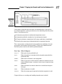
1
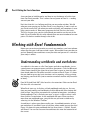
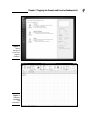
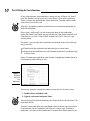
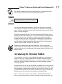
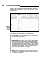
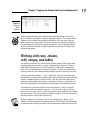
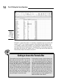
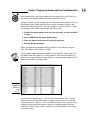
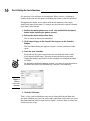
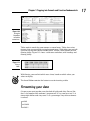
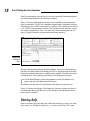
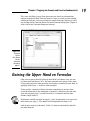
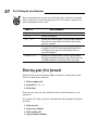
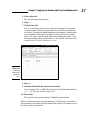
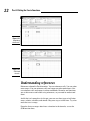
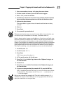
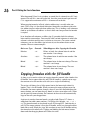
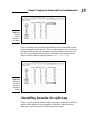
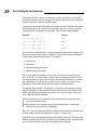
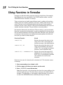
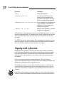
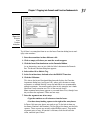
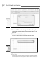
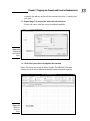
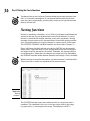
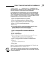
Chapter 1
In This Chapter
▶ Understanding the parts of a worksheet
MA
▶ Getting the skinny on workbooks and worksheets
TE
RI
AL
Tapping into Formula and
Function Fundamentals
▶ Working with cells, ranges, named areas, and tables
▶ Applying formatting
D
▶ Figuring out how to use the Help system
▶ Using functions in formulas
E
GH
▶ Using nested functions
TE
▶ Writing formulas
CO
PY
RI
xcel is to computer programs what a Ferrari is to cars: sleek on the outside and a lot of power under the hood. Excel is also like a truck — it can
handle all your data, lots of it. In fact, in Excel 2010, a single worksheet has
17,179,869,184 places to hold data. Yes, that’s what we said — more than 17
billion data placeholders. And that’s on just one worksheet!
Opening files created in earlier versions of Excel may show just the number of
worksheet rows and columns available in the version the workbook was created with.
Excel is used in all types of businesses. And you know how that’s possible?
By being able to store and work with any kind of data. It doesn’t matter
whether you’re in finance or sales, whether you run an online video store or
organize wilderness trips, or whether you’re charting party RSVPs or tracking the scores of your favorite sports teams — Excel can handle all of it. Its
number-crunching ability is just awesome! And so easy to use!
Just putting a bunch of information on worksheets doesn’t crunch the data or
give you sums, results, or analyses. If you want to just store your data somewhere, you can use Excel or get a database program instead. In this book, we
8
Part I: Putting the Fun in Functions
show you how to build formulas and how to use the dozens of built-in functions that Excel provides. That’s where the real power of Excel is — making
sense of your data.
Don’t fret that this is a challenge and that you may make mistakes. We did
when we were ramping up. Besides, Excel is very forgiving. It won’t crash on
you. Excel usually tells you when you made a mistake, and sometimes it even
helps you to correct it. How many programs do that!? But first the basics.
This first chapter gives you the springboard you need to use the rest of the
book. We wish books like this were around when we were introduced to computers. We had to stumble through a lot of this.
Working with Excel Fundamentals
Before you can write any formulas or crunch any numbers, you have to know
where the data goes. And how to find it again. We wouldn’t want your data to
get lost! Knowing how worksheets store your data and present it is critical to
your analysis efforts.
Understanding workbooks and worksheets
A workbook is the same as a file. Excel opens and closes workbooks, just as
a word processor program opens and closes documents. Click the Microsoft
Office button, found at the upper left of your Excel screen, to view the selections found under the File menu in earlier versions of Excel. Figure 1-1 shows
the new look for accessing basic functions such as opening, saving, printing,
and closing your Excel files (not to mention a number of other nifty functions
to boot!).
Excel 2010 (and Excel 2007) files have the .xlsx extension. Older version Excel
files have the .xls extension.
When Excel starts up, it displays a blank workbook ready for use. If at any
time you need another new workbook, click the Microsoft Office button and
click on New. You will be presented with a plateful of templates, including a
blank workbook. That’s the baby you want, so give it a click to select it and
then click the Create button. A new workbook will open. When you have
more than one workbook open, you pick the one you want to work on by
selecting it in the Windows Taskbar.
A worksheet is where your data actually goes. A workbook contains at least
one worksheet. If you didn’t have at least one, where would you put the data?
Figure 1-2 shows an open workbook that has three sheets — Sheet1, Sheet2,
and Sheet3. You can see these on the worksheet tabs near the bottom left of
the screen.
Chapter 1: Tapping into Formula and Function Fundamentals
Figure 1-1:
Seeing
how to use
basic Excel
program
functions.
Figure 1-2:
Looking at
a workbook
and
worksheets.
9
10
Part I: Putting the Fun in Functions
At any given moment, one worksheet is always on top. In Figure 1-2, Sheet1
is on top. Another way of saying this is that Sheet1 is the active worksheet.
There is always one and only one active worksheet. To make another worksheet active, just click its tab.
Worksheet, spreadsheet, and just plain old sheet are used interchangeably to
mean the worksheet.
Guess what’s really cool? You can change the name of the worksheets.
Names like Sheet1 and Sheet2 are just not exciting. How about Baseball Card
Collection or Last Year’s Taxes? Well, actually Last Year’s Taxes isn’t too
exciting either.
The point is you can give your worksheets meaningful names. You have two
ways to do this:
✓ Double-click the worksheet tab and then type in a new name.
✓ Right-click the worksheet tab, select Rename from the list, and then type
in a new name.
Figure 1-3 shows one worksheet name already changed and another about to
be changed by right-clicking its tab.
Figure 1-3:
Changing
the name
of a
worksheet.
You can try changing a worksheet name on your own. Do it the easy way:
1. Double-click a worksheet’s tab.
2. Type in a new name and press Enter.
You can change the color of worksheet tabs. Right-click the tab and select Tab
Color from the list.
To insert a new worksheet into a workbook, click the Insert sheet tab, which
is located after the last worksheet tab. Figure 1-4 shows how. To delete a
worksheet, just right-click the worksheet’s tab and select Delete from the list.
Chapter 1: Tapping into Formula and Function Fundamentals
Don’t delete a worksheet unless you really mean to. You cannot get it back
after it is gone. It does not go into the Windows Recycle Bin.
Figure 1-4:
Inserting
a new
worksheet.
You can insert many new worksheets. The limit of how many is based on
your computer’s memory, but you should have no problem inserting 200 or
more. Of course we hope you have a good reason for having so many. Which
brings us to the next point.
Worksheets organize your data. Use them wisely and you will find it easy to
manage your data. For example, let’s say you are the boss (we thought you’d
like that!), and you have 30 employees that you are tracking information
on over the course of a year. You may have 30 worksheets — one for each
employee. Or you may have 12 worksheets — one for each month. Or you
may just keep it all on one worksheet. How you use Excel is up to you, but
Excel is ready to handle whatever you throw at it.
New Excel files default to having three worksheets. You can change this
default number on the Personalize tab in the Excel Options dialog box. To display the dialog box, click the Microsoft Office button and then click the Excel
Options button.
Introducing the Formulas Ribbon
It’s a fact of life — or rather, a fact of Microsoft marketing — that each new
release of Office has a slightly different look. The folks at Microsoft went
whole hog with Office 2007. Imagine this — no menus or toolbars. These have
been such staples of Windows applications that only something amazing
could upstage them.
Without further ado, we present the Ribbon. The Ribbon sits at the top of the
application where menus used to unfold and toolbars made their home. A few
items do appear as menu headers along the top of the Excel screen, but they
actually work more like tabs. Click them, and no menus appear. Instead, the
Ribbon presents the items that are related to the clicked header.
Figure 1-5 shows the top part of the screen, in which the Ribbon displays
the items that appear when you click the Formulas header. In the figure, the
11
12
Part I: Putting the Fun in Functions
Ribbon is set to show formula-based methods. Along the left, functions are
categorized. One of the categories is opened to show how you can access a
particular function.
Figure 1-5:
Getting to
know the
Ribbon.
These categories are along the bottom of the Formulas Ribbon:
✓ Function Library: This includes the Function Wizard, the AutoSum feature, and the categorized functions.
✓ Named Cells: These features manage named areas. In fact, the new
Name Manager is here, a brand-new Excel 2007 feature.
✓ Formula Auditing: These features have been through many Excel incarnations, but never before have the features been so prominent. Also
here is the Watch Window, which lets you keep an eye on the values in
designated cells, but within one window. In Figure 1-6 you can see that a
few cells have been assigned to the Watch Window. If any values change,
you can see in the Watch Window. Note how the watched cells are on
sheets that are not the current active sheet. Neat!
✓ Calculation: This is where you manage calculation settings, such as
whether calculation is automatic or manual.
✓ Solutions: Any loaded add-ins that provide further functions appear
here. In Figure 1-5, the Data Analysis Add-in is just another name for the
ever-popular Analysis ToolPak.
Chapter 1: Tapping into Formula and Function Fundamentals
Figure 1-6:
Eyeing the
Watch
Window.
Another new feature that goes hand in hand with the Ribbon is the Quick
Access Toolbar. (So there is a toolbar after all!) In Figure 1-5 the Quick Access
Toolbar sits just under the left side of the Ribbon. On it are icons that perform actions with a single click. The icons are ones you select by using the
Customization tab in the Excel Options dialog box. You can put the toolbar
above or below the Ribbon by right-clicking the Quick Access Toolbar and
choosing the option.
Working with rows, column,
cells, ranges, and tables
A worksheet contains cells. Lots of them. Billions of them. This might seem
unmanageable, but actually it’s pretty straightforward. Figure 1-7 shows a
worksheet filled with data. Use this to look at a worksheet’s components.
Each cell can contain data or a formula. In Figure 1-7, the cells contain data.
Some, or even all, cells could contain formulas, but that’s not the case here.
Columns have letter headers — A, B, C, and so on. You can see these listed
horizontally just above the area where the cells are. After you get past the 26th
column, a double lettering system is used — AA, AB, and so on. After all the
two-letter combinations are used up, a triple-letter scheme is used. Rows are
listed vertically down the left side of the screen and use a numbering system.
You find cells at the intersection of rows and columns. Cell A1 is the cell
at the intersection of column A and row 1. A1 is the cell’s address. There is
always an active cell — that is, a cell in which any entry would go into should
you start typing. The active cell has a border around it. Also, the contents of
the active cell are seen in the Formula Box.
When we speak of, or reference, cell, we are referring to its address. The
address is the intersection of a column and row. To talk about cell D20 means
to talk about the cell that you find at the intersection of column D and row 20.
13
14
Part I: Putting the Fun in Functions
Figure 1-7:
Looking at
what goes
into a worksheet.
In Figure 1-7, the active cell is C7. You have a couple of ways to see this. For
starters, cell C7 has a border around it. Also notice that the column head
C is shaded, as well as row number 7. Just above the column headers are
the Name Box and the Formula Box. The Name Box is all the way to the left
and shows the active cell’s address of C7. To the right of the Name Box, the
Formula Box shows the contents of cell C7.
Getting to know the Formula Bar
Taken together, the Formula Box and the Name
Box make up the Formula Bar. You use the
Formula Bar quite a bit as you work with formulas and functions. The Formula Box is used
to enter and edits formulas. The Formula Box
is the long entry box that starts in the middle of
the bar. When you enter a formula into this box,
you then can click the little check-mark button
to finish the entry. The check-mark button is
only visible when you are entering a formula.
Pressing the Enter key also completes your
entry; clicking the X cancels the entry.
An alternative is to enter a formula directly into
a cell. The Formula Box displays the formula
as it is being entered into the cell. When you
want to see just the contents of a cell that has
a formula, make that cell active and look at its
contents in the Formula Box. Cells that have
formulas do not normally display the formula,
but instead display the result of the formula.
When you want to see the actual formula, the
Formula Box is the place to do it. The Name
Box, on the left side of the Formula Bar, is used
to select named areas in the workbook. This is
addressed further in the material.
Chapter 1: Tapping into Formula and Function Fundamentals
If the Formula Bar is not visible, choose the Advanced tab; in the Display section in the Excel Options dialog box, choose to make it visible.
A range is usually a group of adjacent cells, although noncontiguous cells can
be included in the same range (but that’s mostly for rocket scientists and
those obsessed with calculus). For your purposes, assume a range is a group
of continuous cells. Make a range right now! Here’s how:
1. Position the mouse pointer over the first cell where you wish to define
a range.
2. Press and hold the left mouse button down.
3. Move the pointer to the last cell of your desired area.
4. Release the mouse button.
Figure 1-8 shows what happened when we did this. We selected a range of
cells. The address of this range is A3:D21.
A range address looks like two cell addresses put together, with a colon (:) in
the middle. And that’s what it is! A range address starts with the address of
the cell in the upper left of the range, then has a colon, and then ends with the
address of the cell in the lower right.
Figure 1-8:
Selecting a
range
of cells.
One more detail about ranges — you can give them a name. This is a great
feature because you can think about a range in terms of what it is used for,
instead of what its address is. Also, if we did not take the extra step to assign
a name, the range would be gone as soon as we clicked anywhere on the
worksheet. When a range is given a name, you can repeatedly use the range
by using its name.
15
16
Part I: Putting the Fun in Functions
Say you have a list of clients on a worksheet. What’s easier — thinking of
exactly which cells are occupied, or thinking that there is your list of clients?
Throughout this book, we use areas made of cell addresses and ranges,
which have been given names. It’s time to get your feet wet creating a named
area. Here’s what you do:
1. Position the mouse pointer over a cell, click and hold the left mouse
button down, and drag the pointer around.
2. Release the mouse button when done.
You’ve select an area of the worksheet.
3. Click Name a Range in the Named Cells category on the Formulas
Ribbon.
The New Name dialog box appears. Figure 1-9 shows you how it looks
so far.
4. Name the area if need be.
Excel guesses that you want to name the area with the value it finds
in the top cell of the range. That may or may not be what you want.
Change the name if you need to. In this example, we changed the name
to Clients.
An alternative method to naming an area is to select it, type the name in
the Name Box (left of the Formula Bar), and press the Enter key.
Figure 1-9:
Adding a
name to the
workbook.
5. Click the OK button.
That’s it. Hey, you’re already on your way to being an Excel pro! Now that
you have a named area, you can easily select your data at any time. Just go to
the Name Box and select it from the list. Figure 1-10 shows how we select the
Clients area we set up.
Chapter 1: Tapping into Formula and Function Fundamentals
Figure 1-10:
Using the
Name Box
to find the
named area.
Tables work in much the same manner as named areas. Tables have a few
features that are unavailable to simple named areas. With tables you can indicate that the top row contains header labels. Further, tables default to have
filtering ability. Figure 1-11 shows a table on a worksheet, with headings and
filtering ability.
Figure 1-11:
Trying a
table.
With filtering, you can limit which rows show, based on which values you
select to display.
The Insert Ribbon contains the button to use for inserting a table.
Formatting your data
Of course you want to make your data look all spiffy and shiny. Bosses like
that. Is the number 98.6 someone’s temperature? Is it a score on a test? Is it
ninety-eight dollars and sixty cents? Is it a percentage? Any of these formats
is correct:
✓ 98.6
✓ $98.60
✓ 98.6%
17
18
Part I: Putting the Fun in Functions
Excel lets you format your data in just the way you need. Formatting options
are on the Home Ribbon, in the Number category.
Figure 1-12 shows how formatting helps in the readability and understanding of a worksheet. Cell B1 has a monetary amount and is formatted with the
Accounting style. Cell B2 is formatted as a percent. The actual value in cell B2
is .05. Cell B7 is formatted as currency. The currency format displays a negative value in parentheses. This is just one of the formatting options for currency. Chapter 5 explains further about formatting currency.
Figure 1-12:
Formatting
data.
Besides selecting formatting on the Home Ribbon, you can use the familiar (in
previous versions) Format Cells dialog box. This is the place to go for all your
formatting needs beyond what’s available on the toolbar. You can even create
custom formats. You can display the Format Cells dialog box two ways:
✓ On the Home Ribbon, click the drop-down list from the Number category, and then click More Number Formats.
✓ Right-click any cell and select Format Cells from the pop-up menu.
Figure 1-13 shows the Format Cells dialog box. So many settings are there it
can make your head spin! We discuss this dialog box and formatting more
extensively in Chapter 5.
Getting help
Excel is complex; you can’t deny that. And lucky for all of us, help is just a key
press away. Yes, literally one key press — just press the F1 key. Try it now.
Chapter 1: Tapping into Formula and Function Fundamentals
This starts the Help system. From there you can search on a keyword or
browse through the Help Table of Contents. Later on, when you are working
with Excel functions, you can get help on specific functions directly by clicking the Help on this function link in the Insert Function dialog box. Chapter 2
covers the Insert Function dialog box in detail.
Figure 1-13:
Using the
Format
Cells dialog
box for
advanced
formatting
options.
Gaining the Upper Hand on Formulas
Okay, time to get to the nitty-gritty of what Excel is all about. Sure, you can
just enter data and leave it as is, and even generate some pretty charts from
it. But getting answers from your data, or creating a summary of your data, or
applying what-if tests — all of this takes formulas.
To be specific, a formula in Excel calculates something, or returns some
result based on data in the worksheet. A formula is placed in cells and must
start with an equal sign (=) to tell Excel that it is a formula and not data.
Sounds simple, and it is.
All formulas should start with an equal (=) sign. An alternative is to start a formula with a plus sign (+). This keeps Excel compatible with Lotus 1-2-3.
Look at some very basic formulas. Table 1-1 shows a few formulas and tells
you what they do.
19
20
Part I: Putting the Fun in Functions
We use the word return to refer to what displays after a formula or function
does its thing. So to say the formula returns a 7 is the same as saying the formula calculated the answer to be 7.
Table 1-1
Basic Formulas
Formula
What It Does
=2 + 2
Returns the number 4.
=A1 + A2
Returns the sum of the values in cells A1 and A2, whatever
those values may be. If either A1 or A2 has text in it, then
an error is returned.
=D5
The cell that contains this formula ends up displaying the
value that is in cell D5. If you try to enter this formula into
cell D5 itself, you create a circular reference. That is a
no-no. See Chapter 4.
=SUM(A2:A5)
Returns the sum of the values in cells A2, A3, A4, and A5.
Recall from above the syntax for a range. This formula uses
the SUM function to sum up all the values in the range.
Entering your first formula
Ready to enter your first formula? Make sure Excel is running and a worksheet is in front of you, and then:
1. Click an empty cell.
2. Type this in: = 10 + 10.
3. Press Enter.
That was easy, wasn’t it? You should see the result of the formula — the
number 20.
Try another. This time you create a formula that adds together the value of
two cells:
1. Click any cell.
2. Type in any number.
3. Click another cell.
4. Type in another number.
Chapter 1: Tapping into Formula and Function Fundamentals
5. Click a third cell.
This cell will contain the formula.
6. Type a =.
7. Click the first cell.
This is an important point in the creation of the formula. The formula
is being written by both your keyboard entry and clicking around with
the mouse. The formula should look about half complete, with an equal
sign immediately followed by the address of the cell you just clicked.
Figure 1-14 shows what this looks like. In the example, the value 15 has
been entered into cell B3 and the value 35 into cell B6. The formula was
started in cell E3. Cell E3 so far has =B3 in it.
Figure 1-14:
Entering a
formula that
references
cells.
8. Enter a +.
9. Click the cell that has the second entered value.
In this example, this is cell B6. The formula in cell E3 now looks like this:
=B3 + B6. You can see this is Figure 1-15.
10. Press Enter.
This ends the entry of the function. All done! Congratulations!
Figure 1-16 shows how the example ended up. Cell E3 displays the result of
the calculation. Also notice that the Formula Bar displays the contents of cell
E3, which really is the formula.
21
22
Part I: Putting the Fun in Functions
Figure 1-15:
Completing
the formula.
Figure 1-16:
A finished
formula.
Understanding references
References abound in Excel formulas. You can reference cells. You can reference ranges. You can reference cells and ranges on other worksheets. You
can reference cells and ranges in other workbooks. Formulas and functions
are at their most useful when using references, so you need to understand
them.
And if that isn’t enough to stir the pot, you can use three types of cell references: relative, absolute, and mixed. Okay, one step at a time here. Try a formula that uses a range.
Formulas that use ranges often have a function in the formula, so use the
SUM function here:
Chapter 1: Tapping into Formula and Function Fundamentals
1. Enter some numbers in many cells going down one column.
2. Click in another cell where you want the result to appear.
3. Enter =SUM( to start the function.
4. Click the first cell that has an entered value, hold the left mouse button
down, and drag the mouse pointer over all the cells that have values.
5. Release the mouse button.
The range address appears where the formula and function are being
entered.
6. Enter a ).
7. Press Enter.
8. Give yourself a pat on the back.
Wherever you drag the mouse to enter the range address into a function, you
can also just type in the address of the range, if you know what it is.
Excel is dynamic when it comes to cell addresses. If you have a cell with a formula that references a different cell’s address and you copy the formula from
the first cell to another cell, the address of the reference inside the formula
changes. Excel updates the reference inside the formula to match the number
of rows and/or columns that separate the original cell (where the formula is
being copied from) from the new cell (where the formula is being copied to).
This may be confusing, so try an example so you can see this for yourself:
1. In cell B2, enter 100.
2. In cell C2, enter =B2 * 2.
3. Press Enter.
Cell C2 now returns the value 200.
4. If C2 is not the active cell, click it once.
5. Press Ctrl + C, or click the Copy button in the Clipboard category on
the Home Ribbon.
6. Click cell C3.
7. Press Ctrl + V, or click the Paste button in the Clipboard category on
the Home Ribbon.
8. If you see a strange moving line around cell C2, press the ESC key.
Cell C3 should be the active cell, but if it is not, just click it once. Look at
the Formula Bar. The contents of cell C3 are =B3 * 2, and not the =B2
* 2 that you copied.
Did you see a moving line around a cell? That line’s called a marquee. It’s a
reminder that you are in the middle of a cut or copy operation, and the marquee goes around the cut or copied data.
23
24
Part I: Putting the Fun in Functions
What happened? Excel, in its wisdom, assumed that if a formula in cell C2 references the cell B2 — one cell to the left, then the same formula put into cell
C3 is supposed to reference cell B3 — also one cell to the left.
When copying formulas in Excel, relative addressing is usually what you
want. That’s why it is the default behavior. Sometimes you do not want relative addressing but rather absolute addressing. This is making a cell reference
fixed to an absolute cell address so that it does not change when the formula
is copied.
In an absolute cell reference, a dollar sign ($) precedes both the column
letter and the row number. You can also have a mixed reference in which the
column is absolute and the row is relative or vice versa. To create a mixed
reference, you use the dollar sign in front of just the column letter or row
number. Here are some examples:
Reference Type
Formula
What Happens After Copying the Formula
Relative
=A1
Either, or both, the column letter A and the
row number 1 can change.
Absolute
=$A$1
The column letter A and the row number 1 do
not change.
Mixed
=$A1
The column letter A does not change. The row
number 1 can change.
Mixed
=A$1
The column letter A can change. The row
number 1 does not change.
Copying formulas with the fill handle
As long as we’re on the subject of copying formulas around, take a look at the
fill handle. You’re gonna love this one! The fill handle is a quick way to copy
the contents of a cell to other cells with just a single click and drag.
The active cell always has a little square box in the lower-right side of its
border. That is the fill handle. When you move the mouse pointer over the
fill handle, the mouse pointer changes shape. If you click and hold down the
mouse button, you can now drag up, down, or across over other cells. When
you let go of the mouse button, the contents of the active cell automatically
copy to the cells you dragged over.
A picture is worth a thousand words, so take a look. Figure 1-17 shows a
worksheet that adds some numbers. Cell E4 has this formula: =B4 + C4 +
D4. This formula needs to be placed in cells E5 through E15. Look closely at
cell E4. The mouse pointer is over the fill handle, and it has changed to what
looks like a small, black plus sign. We are about to use the fill handle to drag
that formula to the other cells. Clicking and holding the left mouse button
down and then dragging down to E15 does the trick.
Chapter 1: Tapping into Formula and Function Fundamentals
Figure 1-17:
Getting
ready to
drag the formula down.
Figure 1-18 shows what the worksheet looks like after the fill handle is used
to get the formula into all the cells. This is a real timesaver. Also, you can see
that the formula in each cell of column E correctly references the cells to its
left. This is the intention of using relative referencing. For example, the formula in cell E15 ended up with this formula: =B15 + C15 + D15.
Figure 1-18:
Populating
cells with a
formula by
using the fill
handle.
Assembling formulas the right way
There’s a saying in the computer business: garbage in, garbage out. And that
applies to how formulas are put together. If a formula is constructed the
wrong way, it either returns an incorrect result or an error.
25
26
Part I: Putting the Fun in Functions
Two types of errors can occur in formulas. In one type, Excel can calculate
the formula, but the result is wrong. In the other type, Excel is not able to calculate the formula. Check out both of these.
A formula can work and still produce an incorrect result. Excel does not report
an error because there is no error for it to find. Often this is the result of not
using parentheses properly in the formula. Take a look at some examples:
Formula
Result
=7 + 5 * 20 + 25 / 5
112
=(7 + 5) * 20 + 25 / 5
245
=7 + 5 *( 20 + 25) / 5
52
=(7 + 5 * 20 + 25) / 5
26.4
All of these are valid formulas, but the placement of parentheses makes a difference in the outcome. You must take into account the order of mathematical operators when writing formulas. The order is:
1. Parentheses
2. Exponents
3. Multiplication and division
4. Addition and subtraction
This is a key point of formulas. It is easy to just accept a returned answer.
After all, Excel is so smart. Right? Wrong! Like all computer programs, Excel
can only do what it is told. If you tell it to calculate an incorrect but structurally valid formula, it will do so. So watch your p’s and q’s! Er, rather your
parentheses and mathematical operators when building formulas.
The second type of error is when there is a mistake in the formula or in the
data the formula uses that prevents Excel from calculating the result. Excel
makes your life easier by telling you when such an error occurs. To be precise, it does one of the following:
✓ Excel displays a message when you attempt to enter a formula that is
not constructed correctly.
✓ Excel returns an error message in the cell when there is something
wrong with the result of the calculation.
First, let’s see what happened when we tried to finish entering a formula that
had the wrong number of parentheses. Figure 1-19 shows this.
Excel finds an uneven number of open and closed parentheses. Therefore the
formula cannot work (it does not make sense mathematically), and Excel tells
you so. Watch for these messages; they often offer a solution.
Chapter 1: Tapping into Formula and Function Fundamentals
Figure 1-19:
Getting a
message
from Excel.
On the other side of the fence are errors in returned values. If you got this
far, then the formula’s syntax passed muster, but something went awry nonetheless. Possible errors are:
✓ Attempting to perform a mathematical operation on text
✓ Attempting to divide a number by 0 (a mathematical no-no)
✓ Trying to reference a nonexistent cell, range, worksheet, or workbook
✓ Entering the wrong type of information into an argument function
This is by no means an exhaustive list of possible error conditions, but you
get the idea. So what does Excel do about it? There are a handful of errors
that Excel places into the cell with the problem formula.
Error Type When It Happens
#DIV/0!
When you’re trying to divide by 0
#N/A!
When a formula or a function inside a formula cannot find the
referenced data
#NAME?
When text in a formula is not recognized
#NULL!
When a space was used instead of a comma in formulas that reference multiple ranges; a comma is necessary to separate range
references
#NUM!
When a formula has numeric data that is invalid for the operation type
#REF!
When a reference is invalid
#VALUE!
When the wrong type of operand or function argument is used
Chapter 4 discusses catching and handling formula errors in detail.
27
28
Part I: Putting the Fun in Functions
Using Functions in Formulas
Functions are like little utility programs that do a single thing. For example,
the SUM function sums up numbers, the COUNT function counts, and the
AVERAGE function calculates an average.
There are functions to handle many different needs: working with numbers,
working with text, working with dates and times, working with finance, and
so on. Functions can be combined and nested (one goes inside another).
Functions return a value, and this value can be combined with the results of
another function or formula. The possibilities are nearly endless.
But functions do not exist on their own. They are always a part of a formula.
Now that can mean that the formula is made up completely of the function or
that the formula combines the function with other functions, data, operators,
or references. But functions must follow the formula golden rule: Start with
the equal sign. Look at some examples:
Function/Formula
Result
=SUM(A1:A5)
Returns the sum of the values in the
range A1:A5. This is an example of a
function serving as the whole formula.
=SUM(A1:A5) /B5
Returns the sum of the values in the
range A1:A5 divided by the value in
cell B5. This is an example of mixing a
function’s result with other data.
=SUM(A1:A5) + AVERAGE(B1:B5) Returns the sum of the range A1:A5
added with the average of the range
B1:B5. This is an example of a formula
that combines the result of two
functions.
Ready to write your first formula with a function in it? This function creates
an average:
1. Enter some numbers in a column’s cells.
2. Click an empty cell where you want to see the result.
3. Enter =AVERAGE( to start the function.
Note: Excel presents a list of functions that have the same spelling as the
function name you type. The more letters you type, the shorter the list
becomes. The advantage is, for example, typing the letter A, using the ↓
to select the AVERAGE function, and then pressing the Tab key.
Chapter 1: Tapping into Formula and Function Fundamentals
4. Click the first cell with an entered value and, while holding the mouse
button, drag the mouse pointer over the other cells that have values.
An alternative is to enter the range of those cells.
5. Enter a ).
6. Press Enter.
If all went well, your worksheet should look a little bit like ours, in Figure 1-20.
Cell B10 has the calculated result, but look up at the Formula Bar and you can
see the actual function as it was entered.
Figure 1-20:
Entering the
AVERAGE
function.
Formulas and functions are dependent on the cells and ranges to which
they refer. If you change the data in one of the cells, the result returned by
the function updates. You can try this now. In the example you just did with
making an average, click one of the cells with the values and enter a different
number. The returned average changes.
A formula can consist of nothing but a single function — preceded by an equal
sign, of course!
Looking at what goes into a function
Most functions take inputs — called arguments or parameters — that specify
the data the function is to use. Some functions take no arguments, some take
one, and others take many — it all depends on the function. The argument
list is always enclosed in parentheses following the function name. If there’s
more than one argument, they are separated by commas. Look at a few
examples:
29
30
Part I: Putting the Fun in Functions
Function
Comment
=NOW()
Takes no arguments.
=AVERAGE(A6,A11,B7)
Can take up to 255 arguments.
Here, three cell references are
included as arguments. The arguments are separated by commas.
=AVERAGE(A6:A10,A13:A19,A23:A29) In this example, the arguments are
range references instead of cell
references. The arguments are
separated by commas.
=IPMT(B5, B6, B7, B8)
Requires four arguments. Commas
separate the arguments.
Some functions have required arguments and optional arguments. You must
provide the required ones. The optional ones are well, optional. But you may
want to include them if their presence helps the function return the value
you need.
The IPMT function is a good example. Four arguments are required, and two
more are optional. You can read more about the IPMT function in Chapter 5.
You can read more about function arguments in Chapter 2.
Arguing with a function
Memorizing the arguments that every function takes would be a daunting
task. We can only think that if you could pull that off you could be on television. But back to reality, you don’t have to memorize them because Excel
helps you select what function to use, and then tells you which arguments
are needed.
Figure 1-21 shows the Insert Function dialog box. This great helper is
accessed by clicking the Insert Function button on the Formulas Ribbon. The
dialog box is where you select a function to use.
The dialog box contains a listing of all available functions — and there are
a lot of them! So to make matters easier, the dialog box gives you a way to
search for a function by a keyword, or you can filter the list of functions by
category.
If you know which category a function belongs in, you can click the function
category button in the Formulas Ribbon and select the function from the list.
Chapter 1: Tapping into Formula and Function Fundamentals
Figure 1-21:
Using the
Insert
Function
dialog box.
Try it! Here’s an example of how to use the Insert Function dialog box to multiply a few numbers:
1. Enter three numbers in three different cells.
2. Click an empty cell where you want the result to appear.
3. Click the Insert Function button on the Formulas Ribbon.
As an alternative, you can just click the little fx button on the Formula
Bar. The Insert Function dialog box appears.
4. Select either All or Math & Trig.
5. In the list of functions, find and select the PRODUCT function.
6. Click the OK button.
This closes the Insert Function dialog box and displays the Function
Arguments dialog box (see Figure 1-22), where you can enter as many
arguments as needed. Initially it may not look like it can accommodate
enough arguments. You need to enter three in this example, but it looks
like there is only room for two. This is like musical chairs!
More argument entry boxes appear as you need them. First, though, how
do you enter the argument? There are two ways.
7. Enter the argument one of two ways:
• Type the numbers or cell references into the boxes.
• Use those funny-looking squares to the right of the entry boxes.
In Figure 1-22 two entry boxes are ready to go. To the left of them are
the names Number1 and Number2. To the right of the boxes are the little
squares. These squares are actually called RefEdit controls. They make
argument entry a snap. All you do is click one, click the cell with the
value, and then press Enter.
31
32
Part I: Putting the Fun in Functions
Figure 1-22:
Getting
ready to
enter some
arguments
to the
function.
8. Click the RefEdit control to the right of the Number1 entry box.
The Function Arguments dialog box shrinks to just the size of the
entry box.
9. Click the cell with the first number.
Figure 1-23 shows what the screen looks like at this point.
Figure 1-23:
Using
RefEdit
to enter
arguments.
10. Press Enter.
The Function Arguments dialog box reappears with the argument
entered into the box. The argument is not the value in the cell, but
Chapter 1: Tapping into Formula and Function Fundamentals
instead is the address of the cell that contains the value — exactly what
you want.
11. Repeat Steps 7–9 to enter the other two cell references.
Figure 1-24 shows what the screen should now look like.
Figure 1-24:
Completing
the function
entry.
12. Click OK or press Enter to complete the function.
Figure 1-25 shows the result of all this hoopla. The PRODUCT function
returns the result of the individual numbers being multiplied together.
Figure 1-25:
Math was
never this
easy!
33
34
Part I: Putting the Fun in Functions
You do not have to use the Insert Function dialog box to enter functions into
cells. It is there for convenience. As you become familiar with certain functions that you use repeatedly, you may find it faster to just type the function
directly into the cell.
Nesting functions
Nesting is something a bird does, isn’t it? Well, a bird expert would know the
answer to that one, but we do know how to nest Excel functions. A nested
function is tucked inside another function, as one of its arguments. Nesting
functions let you return results you would have a hard time getting to otherwise. (Nested functions are used in examples in various places in the book.
The COUNTIF, AVERAGE, and MAX functions are discussed in Chapter 9.)
Figure 1-26 shows the daily closing price for the S&P 500, for the month of
August 2009. A possible analysis is to see how many times the closing price
was higher than the average for the month. Therefore, the average needs to
be calculated first, before you can compare any single price. By embedding
the AVERAGE function inside another function, the average is first calculated.
When a function is nested inside another, the inner function is calculated first.
Then that result is used as an argument for the outer function.
Figure 1-26:
Nesting
functions.
The COUNTIF function counts the number of cells in a range that meet a
condition. The condition in this case is that any single value in the range
is greater than (>) the average of the range. The formula in cell D7 is
Chapter 1: Tapping into Formula and Function Fundamentals
=COUNTIF(B5:B25, “>” & AVERAGE(B5:B25)). The AVERAGE function is evaluated first, and then the COUNTIF function is evaluated using the
returned value from the nested function used as an argument.
Nested functions are best entered directly. The Insert Function dialog box
does not make it easy to enter a nested function. Try one. In this example,
you use the AVERAGE function to find the average of the largest values from
two sets of numbers. The nested function in this example is MAX. You enter
the MAX function twice within the AVERAGE function:
1. Enter a few different numbers in one column.
2. Enter a few different numbers in a different column.
3. Click an empty cell where you want the result to appear.
4. Enter =AVERAGE( to start the function entry.
5. Enter MAX(.
6. Click the first cell in the second set of numbers, press the mouse
button, and drag over all the cells of the first set.
The address of this range enters into the MAX function.
7. Enter a closing parenthesis to end the first MAX function.
8. Enter a comma (,).
9. Once again, enter MAX(.
10. Click the first cell in the second set of numbers, press the mouse
button, and drag over all the cells of the second set.
The address of this range enters into the MAX function.
11. Enter a closing parenthesis to end the second MAX function.
12. Enter a ).
This ends the AVERAGE function.
13. Press Enter.
Figure 1-27 shows the result of your nested function. Cell C14 has this formula: =AVERAGE(MAX(B4:B10),MAX(D4:D10)).
When using nested functions, the outer function is preceded with an equal
sign (=) if it is the beginning of the formula. Any nested functions are not preceded with an equal sign.
35
36
Part I: Putting the Fun in Functions
Figure 1-27:
Getting a
result from
nested functions.
You can nest functions up to 64 levels.