1
powerOne® Graph
Version 4.2
© 1997-2005, Infinity Softworks
www.infinitysw.com
2/4/2005
I
powerOne® Graph
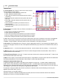
Table of Contents
Part I Using the Calculator
1
1 Interface Overview
................................................................................................................................... 1
Display
.......................................................................................................................................................... 1
Skins
.......................................................................................................................................................... 2
Menus
.......................................................................................................................................................... 2
Pop-up Calculator.......................................................................................................................................................... 3
2 Input Modes ................................................................................................................................... 3
Algebraic Input Mode
.......................................................................................................................................................... 3
Display
......................................................................................................................................................... 4
Implicit Multiplication
......................................................................................................................................................... 5
Preferences ......................................................................................................................................................... 5
Functions
......................................................................................................................................................... 5
RPN Input Mode .......................................................................................................................................................... 9
Display
Stack
......................................................................................................................................................... 9
......................................................................................................................................................... 10
Preferences ......................................................................................................................................................... 10
Functions
......................................................................................................................................................... 10
Order of Operations
..........................................................................................................................................................
Input Mode
14
Display
......................................................................................................................................................... 15
Preferences ......................................................................................................................................................... 15
Functions
......................................................................................................................................................... 16
Chain Input Mode
.......................................................................................................................................................... 17
Display
......................................................................................................................................................... 18
Preferences ......................................................................................................................................................... 18
Functions
......................................................................................................................................................... 19
3 Preferences ................................................................................................................................... 20
Calc Tab
.......................................................................................................................................................... 20
Button Tab
.......................................................................................................................................................... 22
Bar Tab
.......................................................................................................................................................... 22
4 Memory & Storage
................................................................................................................................... 22
My Data
.......................................................................................................................................................... 22
Variables
......................................................................................................................................................... 23
Constants
......................................................................................................................................................... 24
Macros
......................................................................................................................................................... 25
Tables
......................................................................................................................................................... 26
Matrices
......................................................................................................................................................... 28
Sharing Data......................................................................................................................................................... 30
Memory Locations
.......................................................................................................................................................... 31
System Clipboard
.......................................................................................................................................................... 32
History List
.......................................................................................................................................................... 32
Calculation Log .......................................................................................................................................................... 32
Part II Types of Data
1 Booleans
34
................................................................................................................................... 34
2 Integers (Whole
...................................................................................................................................
Number)
34
3 Base Numbers
................................................................................................................................... 34
© 1997-2005, Infinity Softworks
Contents
II
4 Floating Point
...................................................................................................................................
Numbers
34
5 Fractions
................................................................................................................................... 35
6 Dates & Times
................................................................................................................................... 35
7 Complex Numbers
................................................................................................................................... 35
8 Tables & Lists
................................................................................................................................... 35
9 Matrices & Vectors
................................................................................................................................... 35
Part III Subject Areas
37
1 Base Numbers
................................................................................................................................... 37
2 Boolean
................................................................................................................................... 37
3 Calculus
................................................................................................................................... 38
4 Complex Numbers
................................................................................................................................... 38
5 Dates & Times
................................................................................................................................... 39
6 Distribution ................................................................................................................................... 39
7 Finance & Business
................................................................................................................................... 40
8 Fractions
................................................................................................................................... 40
9 Matrices
................................................................................................................................... 41
10 Probability ................................................................................................................................... 41
11 Statistics
................................................................................................................................... 42
12 Tables
................................................................................................................................... 42
13 Trigonometry................................................................................................................................... 43
Part IV Functions
44
1 Symbol Chart
................................................................................................................................... 44
2 A-B
................................................................................................................................... 51
Absolute Value .......................................................................................................................................................... 51
Addition
.......................................................................................................................................................... 51
Adjust Date
.......................................................................................................................................................... 52
Adjust Time
.......................................................................................................................................................... 52
Amortization, End
..........................................................................................................................................................
Balance
53
Amortization, Interest
..........................................................................................................................................................
Paid
54
Amortization, Principal
..........................................................................................................................................................
Paid
55
And
.......................................................................................................................................................... 56
Angle
.......................................................................................................................................................... 57
Angle Symbol .......................................................................................................................................................... 57
Append
.......................................................................................................................................................... 57
Arc-Cosine
.......................................................................................................................................................... 57
Arc-Sine
.......................................................................................................................................................... 58
Arc-Tangent
.......................................................................................................................................................... 58
Augment
.......................................................................................................................................................... 59
Backspace
.......................................................................................................................................................... 59
Binary
.......................................................................................................................................................... 59
Binary, Display As
.......................................................................................................................................................... 60
Binomial Cumulative
..........................................................................................................................................................
Distribution
60
Binomial Probability
..........................................................................................................................................................
Distribution
61
Bond Accrued Interest
.......................................................................................................................................................... 61
© 1997-2005, Infinity Softworks
II
III
powerOne® Graph
Bond Price
.......................................................................................................................................................... 62
Bond Yield
.......................................................................................................................................................... 62
Boolean, Convert
..........................................................................................................................................................
To
62
Braces { }
.......................................................................................................................................................... 63
Brackets [ ]
.......................................................................................................................................................... 63
3 C
................................................................................................................................... 64
Ceiling
.......................................................................................................................................................... 64
Chi-Squared Cumulative
..........................................................................................................................................................
Distribution
65
Chi-Squared Probability
..........................................................................................................................................................
Distribution
65
Choose
.......................................................................................................................................................... 65
Clear
.......................................................................................................................................................... 66
Colon-Equals
.......................................................................................................................................................... 66
Column Norm .......................................................................................................................................................... 66
Combinations .......................................................................................................................................................... 67
Complex Number
..........................................................................................................................................................
Constant
67
Condition
.......................................................................................................................................................... 67
Conjugate
.......................................................................................................................................................... 68
Cosecant
.......................................................................................................................................................... 68
Cosine
.......................................................................................................................................................... 68
Cotangent
.......................................................................................................................................................... 69
Count
.......................................................................................................................................................... 69
Cross Product .......................................................................................................................................................... 70
Cubed Root
.......................................................................................................................................................... 70
Cumulative Standard
..........................................................................................................................................................
Normal Distribution
71
Cumulative Sum.......................................................................................................................................................... 71
4 D-F
................................................................................................................................... 72
Day of Week
.......................................................................................................................................................... 72
Decimal
.......................................................................................................................................................... 72
Decimal Separator
.......................................................................................................................................................... 72
Decimal, Display..........................................................................................................................................................
As
73
Declining Balance
..........................................................................................................................................................
Crossover Depreciation
73
Declining Balance
..........................................................................................................................................................
Depreciation
74
Degrees to DMS..........................................................................................................................................................
Conversion
74
Degrees to Radians
..........................................................................................................................................................
Conversion
75
Derivative
.......................................................................................................................................................... 75
Derivative, Second
.......................................................................................................................................................... 76
Determinant
.......................................................................................................................................................... 76
Difference Between
..........................................................................................................................................................
Dates
77
Dimension
.......................................................................................................................................................... 77
Division
.......................................................................................................................................................... 77
DMS to Degrees..........................................................................................................................................................
Conversion
78
Dot Product
.......................................................................................................................................................... 78
Effective Interest..........................................................................................................................................................
Rate
79
Enter
.......................................................................................................................................................... 79
Equals
.......................................................................................................................................................... 79
Exclusive Or
.......................................................................................................................................................... 80
Exponent
.......................................................................................................................................................... 81
Exponential
.......................................................................................................................................................... 81
F Cumulative Distribution
.......................................................................................................................................................... 82
F Probability Distribution
.......................................................................................................................................................... 82
Factorial
.......................................................................................................................................................... 83
Fill
.......................................................................................................................................................... 83
Floating Point, Convert
..........................................................................................................................................................
To
83
Floor
.......................................................................................................................................................... 84
© 1997-2005, Infinity Softworks
Contents
IV
Fraction, Display..........................................................................................................................................................
As
84
Fractional Part .......................................................................................................................................................... 85
Frobenius Norm.......................................................................................................................................................... 85
Future Value
5 G-H
.......................................................................................................................................................... 86
................................................................................................................................... 86
Geometric Cumulative
..........................................................................................................................................................
Distribution
87
Geometric Probability
..........................................................................................................................................................
Distribution
87
Get Column
.......................................................................................................................................................... 87
Get Date in Decimal
..........................................................................................................................................................
Format
88
Get Hours in Decimal
..........................................................................................................................................................
Format
88
Get Hours in HH.MMSS
..........................................................................................................................................................
Format
89
Get Item
.......................................................................................................................................................... 89
Get Row
.......................................................................................................................................................... 90
Get Time in Decimal
..........................................................................................................................................................
Format
90
Greater Than
.......................................................................................................................................................... 91
Greater Than or ..........................................................................................................................................................
Equal To
91
Greatest Common
..........................................................................................................................................................
Denominator
92
Hexadecimal
.......................................................................................................................................................... 92
Hexadecimal, Display
..........................................................................................................................................................
As
92
History
.......................................................................................................................................................... 93
Hyperbolic Arc-Cosine
.......................................................................................................................................................... 93
Hyperbolic Arc-Sine
.......................................................................................................................................................... 93
Hyperbolic Arc-Tangent
.......................................................................................................................................................... 94
Hyperbolic Cosine
.......................................................................................................................................................... 94
Hyperbolic Sine.......................................................................................................................................................... 94
Hyperbolic Tangent
.......................................................................................................................................................... 95
6 I-N
................................................................................................................................... 95
Identity
.......................................................................................................................................................... 95
If
.......................................................................................................................................................... 95
Integer Part
.......................................................................................................................................................... 96
Integer, Convert..........................................................................................................................................................
To
96
Integral
.......................................................................................................................................................... 97
Interest Rate
.......................................................................................................................................................... 97
Internal Rate of Return
.......................................................................................................................................................... 98
Inverse
.......................................................................................................................................................... 98
Inverse Cumulative
..........................................................................................................................................................
Normal Distribution
99
Last
.......................................................................................................................................................... 99
Least Common Multiple
.......................................................................................................................................................... 99
Less Than
.......................................................................................................................................................... 100
Less Than or Equal
..........................................................................................................................................................
To
100
Logarithm
.......................................................................................................................................................... 101
Make Date from..........................................................................................................................................................
Decimal Format
101
Matrix to Table..........................................................................................................................................................
Conversion
102
Maximum
.......................................................................................................................................................... 102
Maximum, Function
.......................................................................................................................................................... 103
Mean
.......................................................................................................................................................... 104
Median
.......................................................................................................................................................... 104
Memory
.......................................................................................................................................................... 105
Minimum
.......................................................................................................................................................... 105
Minimum, Function
.......................................................................................................................................................... 106
Mixed Fraction,..........................................................................................................................................................
Display As
106
Modified Internal
..........................................................................................................................................................
Rate of Return
107
Modulo Division
.......................................................................................................................................................... 107
Multiplication .......................................................................................................................................................... 108
© 1997-2005, Infinity Softworks
IV
V
powerOne® Graph
Natural Logarithm
.......................................................................................................................................................... 108
Net Future Value
.......................................................................................................................................................... 109
Net Present Value
.......................................................................................................................................................... 110
Net Uniform Series
.......................................................................................................................................................... 110
Nominal Interest
..........................................................................................................................................................
Rate
111
Normal Cumulative
..........................................................................................................................................................
Distribution
112
Normal Probability
..........................................................................................................................................................
Distribution
112
Not
.......................................................................................................................................................... 113
Not Equal
.......................................................................................................................................................... 114
7 O-Q
................................................................................................................................... 114
Occurrences .......................................................................................................................................................... 114
Octal
.......................................................................................................................................................... 115
Octal, Display As
.......................................................................................................................................................... 115
Or
.......................................................................................................................................................... 116
Parentheses
.......................................................................................................................................................... 116
Payback
.......................................................................................................................................................... 117
Payment
.......................................................................................................................................................... 117
Percent
.......................................................................................................................................................... 118
Periods
.......................................................................................................................................................... 119
Permutations .......................................................................................................................................................... 119
Poisson Cumulative
..........................................................................................................................................................
Distribution
120
Poisson Probability
..........................................................................................................................................................
Distribution
120
Polar to Rectangular
..........................................................................................................................................................
Conversion
121
Polar, Convert ..........................................................................................................................................................
To
122
Poly
.......................................................................................................................................................... 122
Power
.......................................................................................................................................................... 122
Power of 10
.......................................................................................................................................................... 123
Present Value .......................................................................................................................................................... 124
Product
.......................................................................................................................................................... 124
Profitability Index
.......................................................................................................................................................... 125
1st Quartile
.......................................................................................................................................................... 125
3rd Quartile
.......................................................................................................................................................... 126
Quotation Marks
.......................................................................................................................................................... 127
8 R
................................................................................................................................... 127
Radians to Degrees
..........................................................................................................................................................
Conversion
127
Random Binomial
..........................................................................................................................................................
Test
127
Random Integer
.......................................................................................................................................................... 128
Random Normal
.......................................................................................................................................................... 129
Random Number
.......................................................................................................................................................... 129
Random Table .......................................................................................................................................................... 130
Random Table ..........................................................................................................................................................
of Integers
130
Reciprocal
.......................................................................................................................................................... 131
Rectangular to..........................................................................................................................................................
Polar Conversion
131
Rectangular, Convert
..........................................................................................................................................................
To
132
Redimension .......................................................................................................................................................... 132
Reduced Row-Echelon
..........................................................................................................................................................
Form
133
Root
.......................................................................................................................................................... 134
Round
.......................................................................................................................................................... 134
Row Add & Multiply
.......................................................................................................................................................... 135
Row Addition .......................................................................................................................................................... 136
Row Multiplication
.......................................................................................................................................................... 136
Row Norm
.......................................................................................................................................................... 136
Row-Echelon Form
.......................................................................................................................................................... 137
© 1997-2005, Infinity Softworks
Contents
9 S
VI
................................................................................................................................... 137
Secant
.......................................................................................................................................................... 137
Semi-Colon
.......................................................................................................................................................... 138
Sequence Evaluation
.......................................................................................................................................................... 138
Shift Left
.......................................................................................................................................................... 139
Shift Right
.......................................................................................................................................................... 139
Show
.......................................................................................................................................................... 139
Sigma
.......................................................................................................................................................... 140
Sign
.......................................................................................................................................................... 140
Sine
.......................................................................................................................................................... 141
Single Payment..........................................................................................................................................................
Future Value
141
Single Payment..........................................................................................................................................................
Present Value
142
Solve
.......................................................................................................................................................... 142
Solving
.......................................................................................................................................................... 143
Sort Ascending.......................................................................................................................................................... 143
Sort Descending
.......................................................................................................................................................... 144
Square
.......................................................................................................................................................... 145
Square Root
.......................................................................................................................................................... 146
Stack
.......................................................................................................................................................... 146
Standard Deviation
.......................................................................................................................................................... 146
Straight Line Depreciation
.......................................................................................................................................................... 147
Student-t Cumulative
..........................................................................................................................................................
Distribution
148
Student-t Probability
..........................................................................................................................................................
Distribution
148
Sub List
.......................................................................................................................................................... 149
Subtraction
.......................................................................................................................................................... 149
Sum of the Year's
..........................................................................................................................................................
Digits Depreciation
150
Sum of x-Squared
.......................................................................................................................................................... 151
Summation
.......................................................................................................................................................... 151
Swap Rows
.......................................................................................................................................................... 152
10 T-Z
................................................................................................................................... 152
Table to Matrix..........................................................................................................................................................
Conversion
152
Tangent
.......................................................................................................................................................... 153
Theta
.......................................................................................................................................................... 153
Today
.......................................................................................................................................................... 153
Total
.......................................................................................................................................................... 153
Transpose
.......................................................................................................................................................... 154
Uniform Series..........................................................................................................................................................
Future Value
154
Uniform Series..........................................................................................................................................................
Present Value
155
Variance
Part V Graphing
.......................................................................................................................................................... 155
156
1 Accessing ................................................................................................................................... 156
2 My Graphs ................................................................................................................................... 157
3 New/Edit Graphs
................................................................................................................................... 157
Function
.......................................................................................................................................................... 158
Parametric
.......................................................................................................................................................... 160
Polar
.......................................................................................................................................................... 161
Sequence
.......................................................................................................................................................... 162
Data
.......................................................................................................................................................... 164
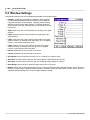
4 Window Settings
................................................................................................................................... 167
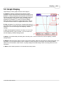
5 Graph Display
................................................................................................................................... 168
© 1997-2005, Infinity Softworks
VI
VII
powerOne® Graph
Analysis Modes
.......................................................................................................................................................... 169
Zooming
.......................................................................................................................................................... 170
6 Examples ................................................................................................................................... 171
Function
.......................................................................................................................................................... 171
Parametric
.......................................................................................................................................................... 173
Polar
.......................................................................................................................................................... 174
Sequence
.......................................................................................................................................................... 176
Scatter Plot
.......................................................................................................................................................... 178
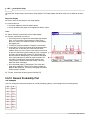
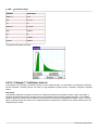
Histogram
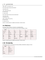
.......................................................................................................................................................... 180
Bar Graph
.......................................................................................................................................................... 183
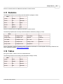
Box Plot
.......................................................................................................................................................... 184
Modified Box Plot
.......................................................................................................................................................... 186
Normal Probability
..........................................................................................................................................................
Plot
187
Graph Names .......................................................................................................................................................... 189
7 Sharing Graphs
................................................................................................................................... 191
Part VI Templates
192
1 Accessing ................................................................................................................................... 192
2 Template List
................................................................................................................................... 192
3 My Templates
................................................................................................................................... 193
4 Using the Templates
................................................................................................................................... 193
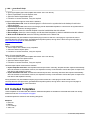
Quick Start Example
.......................................................................................................................................................... 194
Interface Overview
.......................................................................................................................................................... 194
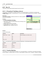
Types of Variable
..........................................................................................................................................................
Data
195
Template Preferences
.......................................................................................................................................................... 196
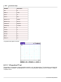
Variable Preferences
.......................................................................................................................................................... 197
Sharing Templates
..........................................................................................................................................................
& Data
198
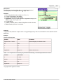
5 Included Templates
................................................................................................................................... 199
One (1)
.......................................................................................................................................................... 201
1-Proportion
.........................................................................................................................................................
Z Confidence Interval
201
1-Variable Statistics
......................................................................................................................................................... 201
1-Proportion
.........................................................................................................................................................
Z Test
203
Two (2)
.......................................................................................................................................................... 205
2-Proportion
.........................................................................................................................................................
Z Confidence Interval
205
2-Proportion
.........................................................................................................................................................
Z Test
206
2-Sample F-Test
......................................................................................................................................................... 207
2-Sample T.........................................................................................................................................................
Confidence Interval
209
2-Sample T.........................................................................................................................................................
Test
211
2-Sample Z.........................................................................................................................................................
Confidence Interval
214
2-Sample Z.........................................................................................................................................................
Test
215
2-Variable Statistics
......................................................................................................................................................... 217
A-D
.......................................................................................................................................................... 220
ANOVA
......................................................................................................................................................... 220
Area
......................................................................................................................................................... 221
Chi-Squared
.........................................................................................................................................................
Test
222
Date
Discount
E-M
......................................................................................................................................................... 223
......................................................................................................................................................... 224
.......................................................................................................................................................... 224
Energy
......................................................................................................................................................... 225
Force
......................................................................................................................................................... 225
Length
......................................................................................................................................................... 226
© 1997-2005, Infinity Softworks
Contents
VIII
Linear Regression
.........................................................................................................................................................
T Test
227
Markup
Mass
N-S
......................................................................................................................................................... 228
......................................................................................................................................................... 229
.......................................................................................................................................................... 229
Percent Change
......................................................................................................................................................... 230
Power
......................................................................................................................................................... 230
Pressure ......................................................................................................................................................... 231
Regressions
......................................................................................................................................................... 232
Sales Tax ......................................................................................................................................................... 234
T
.......................................................................................................................................................... 235
T Confidence
.........................................................................................................................................................
Interval, One-Sample
235
T Test, One-Sample
......................................................................................................................................................... 236
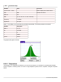
Temperature
......................................................................................................................................................... 237
Time
......................................................................................................................................................... 238
Tip
......................................................................................................................................................... 239
TVM (Time .........................................................................................................................................................
Value of Money)
240
U-Z
.......................................................................................................................................................... 245
Velocity
......................................................................................................................................................... 246
Volume
......................................................................................................................................................... 246
Z Confidence
.........................................................................................................................................................
Interval, One-Sample
247
Z Test, One-Sample
......................................................................................................................................................... 248
6 Creating Templates
................................................................................................................................... 250
Using the Solver
.......................................................................................................................................................... 251
How the Solver..........................................................................................................................................................
Works
252
Solver Limitations
.......................................................................................................................................................... 252
Examples
Inflation
.......................................................................................................................................................... 252
......................................................................................................................................................... 252
Constant Acceleration
......................................................................................................................................................... 253
Home Loan......................................................................................................................................................... 254
"IF" Statements
......................................................................................................................................................... 255
"Solving" Statements
......................................................................................................................................................... 257
Multiple Answers
......................................................................................................................................................... 258
Using Data.........................................................................................................................................................
in Multiple Templates
260
Part VII Appendix
263
1 Calculator Error
...................................................................................................................................
Messages
263
2 Restricted Data
...................................................................................................................................
Names
264
3 Technical Support
................................................................................................................................... 264
4 Printing This
...................................................................................................................................
Manual
264
5 Legal and Disclaimers
................................................................................................................................... 264
Part VIII Index
266
© 1997-2005, Infinity Softworks
VIII
1
powerOne® Graph
1 Using the Calculator
1.1 Interface Overview
This section discusses the interface for powerOne Graph.
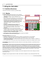
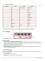
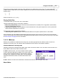
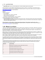
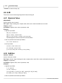
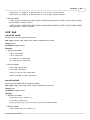
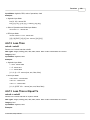
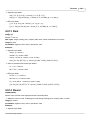
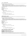
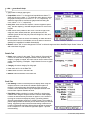
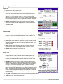
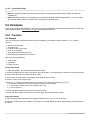
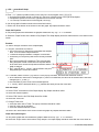
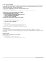
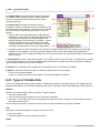
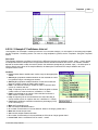
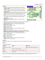
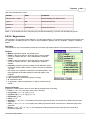
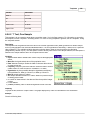
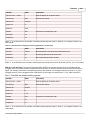
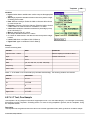
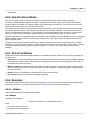
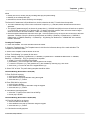
1.1.1 Display
A. powerOne Button (select this button for a list of options):
· Copy: copy contents of view window to the system clipboard.
See Memory & Storage : System Clipboard for more
information.
· Paste: paste the system clipboard to the view window. See
Memory & Storage : System Clipboard for more information.
· Calculation Log: log of calculations similar to a tape. The
Palm OS version records the last 20 calculations (or 10
equation/answer combinations for algebraic input mode).
See Memory & Storage : Calculation Log for more
information.
· Preferences: calculator preferences. See Using the
Calculator : Preferences for more information.
· Skins: change the user interface of the calculator (colors and
layout). See Using the Calculator : Skins for more
information.
· My Data: location to see all calculator data including
constants, macros, and variables. Can also create new data,
whether constants, macros, variables, tables or matrices.
· My Graphs: location to see all graph equations, create new
equations, set window coordinates and graph.
· My Templates: location to see all templates, whether created or pre-installed.
· About powerOne: information about the product.
B. Navigation Buttons (from left to right):
· Data Button: displays My Data. See the Memory & Storage : My Data section for more information.
· Graph Button: displays My Graphs. See the Graphing : My Graphs section for more information.
· Template Button: displays list of available templates similar to My Templates. See the Templates : Template List
section for more information.
· Last Template Button: select to go to the previously used template (only visible when a template has been visited).
C. View Window: displays calculation and status information. See the Using the Calculator : Input Modes section for
more information.
D. Function Bar: consists of 8 lines, each with 5 buttons. Selecting one performs the associated function. Scroll up and
down to see other functions. Buttons can access a function, can display a list of functions or can be associated with a
template. These buttons are programmable and can be set in the Preferences screen. See the Using the Calculator :
Preferences section for more information on setting the function bar. There are also programmable buttons available in
some skins (not pictured). These are not available in the default powerOne Graph skin. Programmable buttons are similar
to the function bar but have a set number of locations and can change in shape, size and direction. These are also
discussed in the Using the Calculator : Preferences section.
E. Function Button: select this button to display a list of function categories. Select a function category to access a
mathematical function.
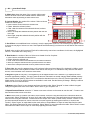
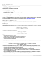
F. Keypad: calculator keypad consists of numbers, basic arithmetic, backspace, clear, positive/negative button and
© 1997-2005, Infinity Softworks
Using the Calculator
2
memory button. Selecting memory shows recall, store and clear. Select store and a memory location to store the view
window's contents to that memory location. Select recall and a memory location to recall that memory location's contents
to the view window. Select clear to clear the memory locations.
· 0-9: numbers 0 through 9.
· decimal separator: separate the whole and decimal portions of the number. Either entered as a period or comma
depending on the system setting for number display format.
· +, –, x, ¸ (plus, minus, times, divide): basic mathematics functions.
· ENT or equals: enter key to evaluate the equation (algebraic input mode), push a value on the stack (RPN input
mode), or complete a calculation (order of operations and chain input modes).
· CE/C: clears the currently entered value on the first selection and all values (entire calculation or history depending on
the input mode) on the second selection.
· MEM: select to access store, recall or clear memory location functionality. See the Memory & Storage : Memory
Locations section for more information.
· +/–: select to change the sign or insert a negative sign depending on the input mode.
· ¬ (backspace arrow): deletes the highlighted area, space before the input cursor, or last entered value depending on
the input mode.
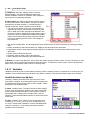
1.1.2 Skins
Skins add a personalized look to the main and pop-up calculators. Some skins offer a different button layout with the
advanced mathematics functions in drop down lists or giving access to programmable buttons for example. Other skins
offer different color schemes.
To download free skins, go to this product's web page at www.infinitysw.com/graph.
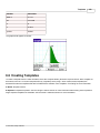
Installing Skins
After downloading a skin from Infinity Softworks' web site and synchronizing it to your device's main memory, run the
application. The skin will be imported automatically. To install a skin from an expansion card, select "Skins" from the
"powerOne" button and choose "Import" to find it.
Changing Skins
To change skins, select "Skins" from the "powerOne" button. Choose the desired skin and then select "OK". The
calculator display will change automatically. "<Default>" is the original display that came with your product.
Deleting Skins
To delete a skin, select "Skins" from the "powerOne" button. Choose the desired skin and select "Delete". The default
skin cannot be deleted.
Problems with Skins
If there is a device problem when working in a skin, it is possible to return to the default skin when launching the
software. To do so, hold the down scroll or 5-way navigation button when starting the software.
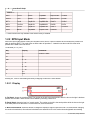
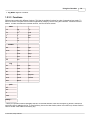
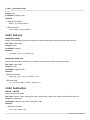
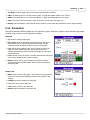
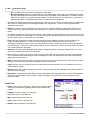
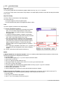
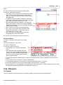
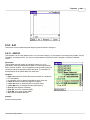
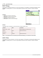
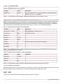
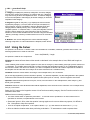
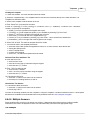
1.1.3 Menus
Choosing the menu button to the lower, left-hand corner of the Graffiti input area accesses the menus. Standard PalmOS
edit choices, Graffiti help, Preferences, and application information can be accessed from here.
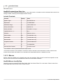
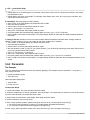
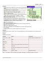
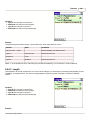
The Edit menu:
·
·
·
·
·
·
·
Undo: shortcut U, undo the last cut/copy/paste or entry in the field. Algebraic and RPN input modes only.
Cut: shortcut X, cut the selected text to the clipboard.
Copy: shortcut C, copy the selected text to the clipboard.
Paste: shortcut P, paste the selected text from the clipboard to the entry line.
Select All: shortcut S, selects all text in the entry line. Algebraic and RPN input modes only.
Keyboard: shortcut K, displays the Palm OS keyboard for data entry. Algebraic and RPN input modes only.
Graffiti Help: shortcut G, help with Graffiti keystrokes.
© 1997-2005, Infinity Softworks
3
powerOne® Graph
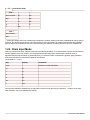
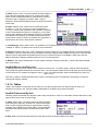
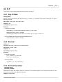
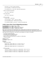
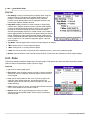
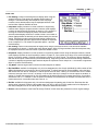
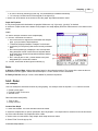
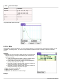
The Options menu:
· Preferences: shortcut R, displays the calculator preferences.
· Clear Memory: shortcut Y, clear the calculator's 10 memory locations.
· About powerOne: displays company information.
Copy, paste, error and keystroke help, preferences and the about screen can all be reached from the powerOne button as
well.
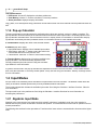
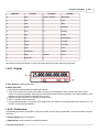
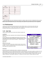
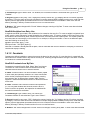
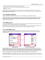
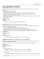
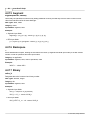
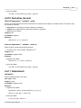
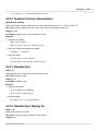
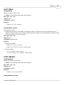
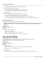
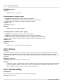
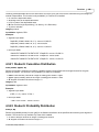
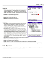
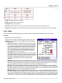
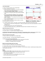
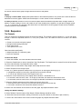
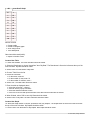
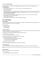
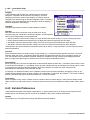
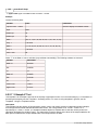
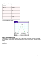
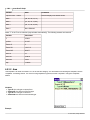
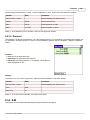
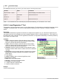
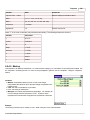
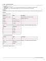
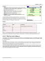
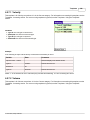
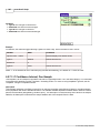
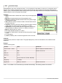
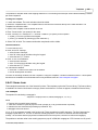
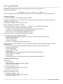
1.1.4 Pop-up Calculator
The pop-up calculator is used throughout the application when values are required, such as in a table or template. The
pop-up calculator functions similarly to the main calculator and offers the same input modes. Functionality specific to the
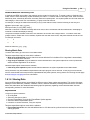
pop-up calculator is detailed here. See the Interface Overview : Display section for information on shared main and popup calculator functionality and the Input Modes section for information specific to each available input mode.
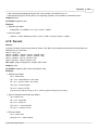
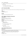
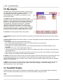
A. Variable Name: displays the name of the selected variable.
B. Buttons (from left to right):
· Input Mode Button: displays a list of available input modes.
· Save Button: select the "ü" button to store the value in the
view window and return to the previous view.
· Cancel Button: select the "x" button to return without storing.
C. Function Button: displays a list of functions available in the
pop-up calculator. This list's functionality depends on the
currently selected input mode. See the Using the Calculator :
Input Modes for more information.
In general, entries made in the pop-up calculator are separate from those in the main calculator. To move data between
them, store the information in a memory location (MEM : Store). See the Using the Calculator : Memory & Storage section
for more information.
1.2 Input Modes
An input mode is the method by which calculations are performed in the main calculator. The different modes reflect the
variety of calculation methods performed by currently available hardware calculators.
The currently selected skin dictates the available input modes. See Using the Calculator : Interface Overview : Skins for
more information.
The input mode is set in the preferences. See Using the Calculator : Interface Overview for more information on
accessing the preferences.
1.2.1 Algebraic Input Mode
Algebraic is the most common input mode used with scientific calculators. In algebraic mode, the entire equation is
entered than the [ENT] button is selected to evaluate the equation. This mode follows common order of operation rules for
function precedence.
The following chart outlines function precedence. Functions with a lower order are executed before functions with a higher
order:
© 1997-2005, Infinity Softworks
Using the Calculator
Order
#Function
1
Negative (-x)
2
Powers and roots
3
Multiplication, division, and percentages
4
Addition and subtraction
5
Relationship operations (>, <=)
6
Logic or Boolean operations (or, and)
4
For example, 27 + 3 x 8.5 is evaluated as (3 x 8.5) + 27:
Key
Display
Comments
CLR
27
27
+
27+
3
27+3
x
27+3*
8.5
27+3*8.5
ENT
52.5
Enter evaluates the entire equation at once
1.2.1.1 Display
A. History List: shows the past 4 equation/answer combinations. Select the button to see the list. It is organized the
same as in B below.
B. Last Equation/Answer: the top line shows the last equation entered, the lower line shows the last result. To recall the
last equation entered to the entry line, select it. To recall the last result as the number of decimal places displayed on the
screen, select the last answer's value (19 in the picture). Selecting the location designation (H1 in this picture) does one
of three things. If the designation starts with H, selecting it recalls the full precision to the entry line for use in the next
calculation. If the designation starts with M, selecting it displays the matrix editor. If the designation starts with T, selecting
it displays the table editor.
C. Base-Fraction Mode: select this button to change number base or to display results as fractions. For instance, after
changing the mode to hexadecimal, all entries and calculations are assumed to be hexadecimal unless designated as
something else. See the Using the Calculator : Types of Data section for detailed information on each mode:
· Fraction: results are displayed as fractions (e.g, 3/4).
· Mix Fraction: results are displayed as mixed fractions (e.g, 2+4/5).
· Binary: results are displayed as binary numbers (e.g, 11001_b) and values entered into the entry line are treated as
binary numbers.
© 1997-2005, Infinity Softworks
5
powerOne® Graph
· Octal: results are displayed as octal numbers (e.g, 845_o) and values entered into the entry line are treated as octal
numbers.
· Decimal: decimal mode is the default mode for entering values, complex numbers, etc (e.g, 8.35, 90_d).
· Hexadecimal: results are displayed as hexadecimal numbers (e.g, 8F_h, 0AC_h) and values entered into the entry
line are treated as hexadecimal numbers. Hexadecimal numbers that begin with a letter must start with 0 (e.g, 0AC_h
instead of AC_h).
D. Entry Line: enter the calculation on the line. If the calculation is longer than a single line, a scroll bar will appear (not
pictured here).
1.2.1.2 Implicit Multiplication
In certain cases, implicit multiplication is available. Implicit multiplication is where 2 times x is entered as 2x. In algebraic
input mode, multiplication is assumed if the math symbol is missing.
The following examples will support implicit multiplication:
· 2x : assumed to be 2 * x.
· 2 x : (note: the space between 2 and x), assumed to be 2 * x.
· a b : (note: the space between a and b), assumed to be a * b.
· 3(x+2) : assumed to be 3 * (x + 2).
2
· {1; 2; 3}x^2 : assumed to be list {1; 2; 3} * x .
· 4sin(25) : assumes 4 * sin(25).
The following examples will not support implicit multiplication
· ab : this is not a * b, but instead the variable 'ab'. (Enter a multiplication symbol or space between a and b to handle
correctly.)
· a2 : this is not a * 2, but instead the variable 'a2'. (Enter a multiplication symbol or space between a and b to handle
correctly.)
· a(2+3) : this is not a * (2+3), but instead the function call a(5). (A number before a parentheses is allowed but a
variable before a parentheses is not. Also, a space between a and (2+3) would also be considered a function call.)
1.2.1.3 Preferences
The following preferences are available in algebraic input mode. See the Using the Calculator : Preferences section for
more information:
· Decimal Setting: float or 0 through 11.
· Display Mode: normal, scientific or engineering notation.
· Complex Type: auto-detect, always rectangular, always polar.
· Complex Frmt: display as (a;b) | (r;@t) format or (a+b*i) | (r*e^t*i) format.
· Unary Op: -2^2 equals -4 (like TI) or 4 (like HP).
· Trig Mode: degrees or radians.
1.2.1.4 Functions
Different input modes offer different functions. This lists the available functions for algebraic input mode. To learn how to
see a complete list of functions organized by category, See the Using the Calculator : Interface Overview section. To
learn more about an individual function, see the Functions section.
© 1997-2005, Infinity Softworks
Using the Calculator
math
1/x
x
log
Öy
x
%x
10
yx
x
2
gcd
ln
Öx
lcm
3
Öx
solve
;
iPart
rnd
toFloat
(
fPart
degs
®frac
)
floor
dms
®mFrac
EE
ceil
toBool
abs
sign
toInt
sin
sinh
sec
cos
cosh
csc
tan
tanh
cot
asin
asinh
degrees
acos
acosh
radians
atan
atanh
e
x
mod
number
trig
prob
nPr
randT
nCr
randTInt
x!
RandNorm *
rand
RandBin *
randInt
stats
{ } (tbl)
median
variance
countX
min
varianceP
sumX
max
sigma
sumX2
stdDev
seq
mean
stdDevP
prod
© 1997-2005, Infinity Softworks
6
powerOne® Graph
7
distr
nDist
NormalCDF *
fCDF *
invNorm
NormalPDF *
fPDF *
BinomCDF *
GeometCDF *
chiCDF *
BinomPDF *
GeometPDF *
chiPDF *
PoissonCDF *
tCDF *
PoissonPDF *
tPDF *
* These functions are only available if the statistics library is installed.
cmplx
i
real
@
theta
conj
toRect
imag
toPolar
calc
'x'
fnInt
""
fMax
nDeriv
fMin
nDeriv2
matrix
[ ] (mtrx)
rref
rNorm
min
*row+
dim
{ } (tbl)
trans
cNorm
max
fill
getItem
identity
cond
rowSwap
augment
getRow
det
cumSum
cross
row+
append
getCol
ref
norm
dot
row*
redim
x
-1
cnst **
New Constant...
c
Me
Edit...
ec
Mn
e
g
Mp
i
G
NA
pi
k
R
© 1997-2005, Infinity Softworks
Using the Calculator
8
vars **
New Variable...
New Table...
New Matrix...
Edit...
=
macro **
New Macro...
Edit...
:=
** These lists change when new constants, variables and macros are created, inserting new items in alphabetical order at
the top of the list. See the Memory & Storage : My Data section for more information on creating new constants, variables
and macros.
bool
==
<=
||
<>
>=
##
<
!x
if
>
&&
choose
~x
_b
b
A
&
_o
o
B
|
_d
d
C
#
_h
h
D
dev
<<
E
>>
F
date
adjDate
getDate
adjTime
getTime
makeDate
HRS
weekDay
HMS
dDays
today
© 1997-2005, Infinity Softworks
9
powerOne® Graph
finance ***
IntEff
TvmFV
BondY
DepDBBV
DepSOYDBV
CfoNUS
IntNom
TvmI
BondA
DepDBDV
DepSOYDDV
CfoPbk
SPFV
TvmN
DepSLDA
DepDBSLDA
CfoNPV
CfoProf
SPPV
TvmPmt
DepSLBV
DepDBSLBV
CfoIRR
CfoTot
USFV
TvmPV
DepSLDV
DepDBSLDV
CfoNFV
CfoCount
USPV
BondP
DepDBDA
DepSOYDDA
CfoMIRR
*** These functions are only available if the finance library is installed.
1.2.2 RPN Input Mode
RPN is the input mode familiar to many HP calculator users. RPN is a post-fix notation where numbers are pushed on a
stack by pressing [ENT]. This mode does not follow order of operations – instead it uses the model of the last value
pushed on the stack is the first one off.
To calculate (27 + 3) x 8.5:
Key
Display
CE/C
Comments
Clears the stack.
27
27
ENT
0: 27
3
1: 27
3
+
0: 30
8.5
1: 30
8.5
x
255
Entering 8.5, 3 and 27 then adding and finally multiplying will derive the same answer.
1.2.2.1 Display
A. Full Stack: shows the complete stack. The number to the left is the stack position while the item to the right is the data
pushed onto the stack. Stack functions are available by selecting a stack item.
B. Partial Stack: shows the last 2 to 3 stack entries. The number to the left is the stack position while the item to the right
is the data pushed onto the stack. For stack functions, select a stack item.
C. Base-Fraction Mode: select this button to change the display to support a specific mode. For instance after changing
the mode to hexadecimal, all entries and calculations are assumed to be in this mode unless designated as something
© 1997-2005, Infinity Softworks
Using the Calculator
10
else. See the Using the Calculator : Types of Data section for detailed information on each mode:
· Fraction: results are displayed as fractions (e.g, 3/4).
· Mix Fraction: results are displayed as mixed fractions (e.g, 2+4/5).
· Binary: results are displayed as binary numbers (e.g, 11001_b) and values entered into the entry line are treated as
binary numbers.
· Octal: results are displayed as octal numbers (e.g, 845_o) and values entered into the entry line are treated as octal
numbers.
· Decimal: decimal mode is the default mode for entering values, complex numbers, etc (e.g, 8.35, 90_d).
· Hexadecimal: results are displayed as hexadecimal numbers (e.g, 8F_h, 0AC_h) and values entered into the entry
line are treated as hexadecimal numbers. Hexadecimal numbers that begin with a letter must start with 0 (e.g, 0AC_h
instead of AC_h).
D. Entry Line: enter values on the line. If the value is longer than a single line, a scroll bar will appear (not pictured here).
1.2.2.2 Stack
There are special functions for manipulating the stack. These functions can be reached by tapping an item pushed onto
the stack or choosing the category Stack from the function list and then selecting the desired function. If an item is
selected on the stack, the function selected will adjust based on that item. If a stack function is selected from the function
list the first item on the stack will be the focal point.
· Drop: deletes the item.
· Duplicate (dup): copies the item into register 0 (view window/entry line), pushing all others up.
· Move: removes the item from its location in the stack and places it in register 0 (view window/entry line).
· Rotate (rot): moves the stack in a clockwise direction.
· Rotate Rvrs (rotr): moves the stack in a reverse or counter-clockwise direction.
· Swap: swaps the item with the contents of register 0 (view window/entry line).
1.2.2.3 Preferences
The following preferences are available in RPN input mode. See the Using the Calculator : Preferences section for more
information:
· Stack Size: 4, 11 or max registers. Includes register 0 (view window/entry line). The maximum number of registers
available is 64.
· Enter Mode: HP 48 where enter does not push a duplicate of the view window/entry line onto the stack or All Other
HP calculators that do push a duplicate of the view window/entry line onto the stack.
· Decimal Setting: float or 0 through 11.
· Display Mode: normal, scientific or engineering notation.
· Complex Type: auto-detect, always rectangular, always polar.
· Complex Frmt: display as (a;b) | (r;@t) format or (a+b*i) | (r*e^t*i) format.
· Trig Mode: degrees or radians.
1.2.2.4 Functions
Different input modes offer different functions. This lists the available functions for RPN input mode. To learn how to see a
complete list of functions organized by category, See the Using the Calculator : Interface Overview section. To learn more
about an individual function, see the Functions section.
© 1997-2005, Infinity Softworks
powerOne® Graph
11
math
1/x
x
log
Öy
x
%x
10
yx
x
2
gcd
ln
Öx
lcm
e
x
mod
3
Öx
number
last
EE
ceil
toBool
show
abs
sign
toInt
;
iPart
rnd
toFloat
(
fPart
degs
®frac
)
floor
dms
®mFrac
sin
sinh
sec
cos
cosh
csc
tan
tanh
cot
asin
asinh
degrees
acos
acosh
radians
atan
atanh
trig
prob
nPr
randT
nCr
randTInt
x!
RandNorm *
rand
RandBin *
randInt
stack
drop
rotr
dup
swap
move
stack
rot
© 1997-2005, Infinity Softworks
Using the Calculator
stats
{ } (tbl)
median
variance
countX
min
varianceP
sumX
max
sigma
sumX2
stdDev
seq
mean
stdDevP
prod
nDist
NormalCDF *
fCDF *
invNorm
NormalPDF *
fPDF *
BinomCDF *
GeometCDF *
chiCDF *
BinomPDF *
GeometPDF *
chiPDF *
PoissonCDF *
tCDF *
PoissonPDF *
tPDF *
distr
* These functions are only available if the statistics library is installed.
cmplx
i
real
@
theta
conj
toRect
imag
toPolar
calc
'x'
fnInt
""
fMax
nDeriv
fMin
nDeriv2
matrix
[ ] (mtrx)
rref
rNorm
min
*row+
dim
{ } (tbl)
trans
cNorm
max
fill
getItem
identity
cond
rowSwap
augment
getRow
det
cumSum
cross
row+
append
getCol
ref
norm
dot
row*
redim
x
-1
© 1997-2005, Infinity Softworks
12
13
powerOne® Graph
cnst **
New Constant...
c
Me
Edit...
ec
Mn
e
g
Mp
i
G
NA
pi
k
R
vars **
New Variable...
New Table...
New Matrix...
Edit...
=
** These lists change when new constants and variables are created, inserting new items in alphabetical order at the top
of the list. See the Memory & Storage : My Data section for more information on creating new constants and variables.
Macros defined as constants will not show in the Constants list.
bool
==
<=
||
<>
>=
##
<
!x
>
&&
dev
~x
_b
b
A
&
_o
o
B
|
_d
d
C
#
_h
h
D
<<
E
>>
F
date
adjDate
getDate
adjTime
getTime
makeDate
HRS
weekDay
HMS
dDays
today
© 1997-2005, Infinity Softworks
Using the Calculator
14
finance ***
IntEff
TvmFV
BondY
DepDBBV
DepSOYDBV
CfoNUS
IntNom
TvmI
BondA
DepDBDV
DepSOYDDV
CfoPbk
SPFV
TvmN
DepSLDA
DepDBSLDA
CfoNPV
CfoProf
SPPV
TvmPmt
DepSLBV
DepDBSLBV
CfoIRR
CfoTot
USFV
TvmPV
DepSLDV
DepDBSLDV
CfoNFV
CfoCount
USPV
BondP
DepDBDA
DepSOYDDA
CfoMIRR
*** These functions are only available if the finance library is installed.
1.2.3 Order of Operations Input Mode
Order of operations is a standard calculator mode where only the currently entered number appears in the view window.
This mode follows standard entry where numbers are entered in order of appearance and a final calculation is performed
when [=] is selected. As the name indicates, it follows standard order of operations rules.
The following chart outlines precedence:
Order
#Function
1
Negative (-x)
2
Powers and roots
3
Multiplication, division, and percentages
4
Addition and subtraction
5
Relationship operations (>, <=)
6
Logic or Boolean operations (or, and)
To calculate 27 + 3 x 8.5:
Key
Display
CE/C
Comments
Clears the current calculation.
27
27
+
27
3
3
x
3
8.5
8.5
=
52.5
On Palm OS handhelds, Graffiti® entry is supported for both the main and pop-up calculators. To learn how to draw
each character, see your handheld user manual.
© 1997-2005, Infinity Softworks
15
powerOne® Graph
Character
Function
Character
Function
0
Zero
<back> <space>
Backspace
1
One
c
C/CE
2
Two
+
Add
3
Three
–
Subtract
4
Four
x *
Multiply
5
Five
/
Divide
6
Six
=
Equals/Enter
7
Seven
(
Lt Paren
8
Eight
)
Rt Paren
9
Nine
s
Store
. ,
Decimal Pt
r
Recall
n
Sign
<return>
Save
e
Exponent
Note that the Graffiti shift indicator is in the view window both on the main and pop-up calculators.
1.2.3.1 Display
A. View Window: number display area.
B. Status Indicators:
· Shift Indicator: Standard Palm OS Graffiti shift indicator.
· Clear: Clear serves two functions in this mode. Selecting it once displays the clear indicator and clears only the
number currently being entered. Selecting it the second time clears the entire calculation. If the status indicator "clear"
appears, the currently entered number has been cleared.
· Deg/Rad: Whether calculator is in degrees or radians mode.
· OOO: Currently in order of operations input mode.
· (0): parentheses indicator. The number in the middle shows the number of left parentheses that are still open (i.e., do
not have a closing right parenthesis).
1.2.3.2 Preferences
The following preferences are available in order of operations input mode. See the Using the Calculator : Preferences
section for more information:
· Decimal Setting: float or 0 through 11.
· Display Mode: normal, scientific or engineering notation.
© 1997-2005, Infinity Softworks
Using the Calculator
16
· Trig Mode: degrees or radians.
1.2.3.3 Functions
Different input modes offer different functions. This lists the available functions for order of operations input mode. To
learn how to see a complete list of functions organized by category, see the Using the Calculator : Interface Overview
section. To learn more about an individual function, see the Functions section.
math
1/x
%x
10
yx
x
ln
e
x
log
x
Öy
x
mod
2
gcd
Öx
lcm
3
Öx
number
last
abs
sign
show
iPart
rnd
(
fPart
degs
)
floor
dms
EE
ceil
trig
sin
sinh
sec
cos
cosh
csc
tan
tanh
cot
asin
asinh
degrees
acos
acosh
radians
atan
atanh
prob
nPr
nCr
x!
rand
history *
* History is a special function that displays the last 10 recorded answers. Each time the equals [=] button is selected, a
new history item is added to the list. To recall a history item to the view window, select it from the list (or choose function
Last for the last value added to the history list).
© 1997-2005, Infinity Softworks
17
powerOne® Graph
cnst **
New Constant...
ec
Mn
Edit...
g
Mp
e
G
NA
pi
k
R
c
Me
vars **
New Variable...
Edit...
** These lists change when new constants and variables are created, inserting new items in alphabetical order at the top
of the list. See the Memory & Storage : My Data section for more information on creating new constants and variables.
Macros defined as constants will not show in the Constants list. Matrices and tables will not show in the Variables list.
1.2.4 Chain Input Mode
Chain input mode is the most common mode found in financial calculators. It is a mode where only the currently entered
number appears in the view window. This mode follows standard entry where numbers are entered in order of
appearance and a final calculation is performed when [=] is selected. Order of operations is ignored, opting instead to
evaluate as numbers are entered and operands are selected.
To calculate 27 + 3 x 8.5:
Key
Display
CE/C
Comments
Clears the current calculation.
27
27
+
27
3
3
x
30
8.5
8.5
=
255
On Palm OS handhelds, Graffiti® entry is supported for both the main and pop-up calculators. To learn how to draw
each character, see your handheld user manual.
© 1997-2005, Infinity Softworks
Using the Calculator
Character
Function
Character
18
Function
0
Zero
<back> <space>
Backspace
1
One
c
C/CE
2
Two
+
Add
3
Three
–
Subtract
4
Four
x *
Multiply
5
Five
/
Divide
6
Six
=
Equals/Enter
7
Seven
(
Lt Paren
8
Eight
)
Rt Paren
9
Nine
s
Store
. ,
Decimal Pt
r
Recall
n
Sign
<return>
Save
e
Exponent
Note that the Graffiti shift indicator is in the view window both on the main and pop-up calculators.
1.2.4.1 Display
A. View Window: number display area.
B. Status Indicators:
· Shift Indicator: Standard Palm OS Graffiti shift indicator.
· Clear: Clear serves two functions in this mode. Selecting it once displays the clear indicator and clears only the
number currently being entered. Selecting it the second time clears the entire calculation. If the status indicator "clear"
appears, the currently entered number has been cleared.
· Deg/Rad: Whether calculator is in degrees or radians mode.
· Chain: Currently in chain input mode.
· (0): parentheses indicator. The number in the middle shows the number of left parentheses that are still open (i.e., do
not have a closing right parenthesis).
1.2.4.2 Preferences
The following preferences are available in chain input mode. See the Using the Calculator : Preferences section for more
information:
· Decimal Setting: float or 0 through 11.
· Display Mode: normal, scientific or engineering notation.
© 1997-2005, Infinity Softworks
powerOne® Graph
19
· Trig Mode: degrees or radians.
1.2.4.3 Functions
Different input modes offer different functions. This lists the available functions for chain input mode. To learn how to see
a complete list of functions organized by category, see the Using the Calculator : Interface Overview section. To learn
more about an individual function, see the Functions section.
math
1/x
%x
y
10
x
x
Öy
x
mod
2
gcd
Öx
lcm
x
ln
e
x
log
3
Öx
number
last
abs
sign
show
iPart
rnd
(
fPart
degs
)
floor
dms
EE
ceil
trig
sin
sinh
sec
cos
cosh
csc
tan
tanh
cot
asin
asinh
degrees
acos
acosh
radians
atan
atanh
prob
nPr
nCr
x!
rand
history *
* History is a special function that displays the last 10 recorded answers. Each time the equals [=] button is selected, a
new history item is added to the list. To recall a history item to the view window, select it from the list (or choose function
Last for the last value added to the history list).
© 1997-2005, Infinity Softworks
Using the Calculator
20
cnst **
New Constant...
ec
Mn
Edit...
g
Mp
e
G
NA
pi
k
R
c
Me
vars **
New Variable...
Edit...
** These lists change when new constants and variables are created, inserting new items in alphabetical order at the top
of the list. See the Memory & Storage : My Data section for more information on creating new constants and variables.
Macros defined as constants will not show in the Constants list. Matrices and tables will not show in the Variables list.
1.3 Preferences
Preferences are used to store information about how the calculator functions, set the function bar and set the
programmable buttons. The "Bar" and/or "Button" tabs only appear if the selected skin offers these functions.
Access the preferences by selecting "powerOne" then "Preferences".
1.3.1 Calc Tab
Display changes depending on the input mode selected. Options are:
Input Mode
[algebraic, RPN, order of operations, chain modes] the currently selected
input mode.
All input modes may not be available with all skins. For more on each
input mode, see the Using the Calculator : Input Modes section. To learn
more about skins, see the Using the Calculator : Interface Overview :
Skins section.
Stack Size
[RPN] size of the stack.
The stack can either be 4 items tall (3 locations and the entry line/view
window), 11 items (10 locations and the entry line/view window) or max
items high. Max is restricted to 64 items.
Enter Mode
[RPN] how the stack is handled when [ENT] is selected in RPN input mode.
HP48 calculators treat "Enter" differently than all other HP RPN calculators. On the HP48, [3] [ENT] [+] results in an error
because not enough items are pushed onto the stack. On other HP calculators, the same sequence results in 6 (3 + 3),
since it pushes 3 into the first register without removing it from the entry line/view window. Choose HP 48 to match the
HP48 or All Others for the alternative sequence. For reference, previous versions of Infinity Softworks' financial
© 1997-2005, Infinity Softworks
21
powerOne® Graph
calculators only offered a mode equivalent to the HP48.
Decimal Setting
[algebraic, RPN, order of operations, chain modes] number of decimal places to display.
Float shows all available decimal places. 0 through 11 shows that many decimal places. With very large numbers, fewer
decimal places may be displayed because of the total number of places available to show in the view window. In addition,
the Show function displays all available decimal places until the next entry is made. This can be used to quickly see all
available decimal places when the decimal setting is not set to float.
Display Mode
[algebraic, RPN, order of operations, chain modes] display numbers in normal, scientific or engineering notation.
Normal mode displays numbers as would normally be written on paper or, if the number is very large or very small, in
scientific notation. Scientific mode displays numbers as two parts -- the significant digits with one digit before the decimal
and the exponent (e.g, 3.45e67). The number of places displayed after the decimal point is determined by the decimal
setting. Engineering mode also displays numbers in two parts -- the significant digits and the exponent that is always a
multiple of 3 (e.g, 34.567e12). The number of significant digits is 1 plus the decimal setting.
Complex Type
[algebraic, RPN] sets the type of complex number to be displayed.
Choose between auto, rectangular or polar. In auto mode, the calculator will display a complex number answer in
rectangular or polar format depending on the format preferred by the last operation performed. If set to rectangular,
answers will always return in rectangular format [either (a;b) or (a+b*i) format]. If set to polar, answers will always return in
polar format [either (r;@t) or (r*e^t*i) format]. See the Types of Data : Complex Numbers section for more information on
complex numbers.
Complex Frmt
[algebraic, RPN] sets the format in which a complex number is displayed.
Complex numbers can be displayed and entered in a format standard to Infinity Softworks [ (a;b) or (r;@t for rectangular
and polar, respectively] or can be displayed in a standard mathematical format [ (a+b*i) or (r*e^t*i) for rectangular and
polar, respectively]. See the Types of Data : Complex Numbers section for more information on complex numbers.
Unary Op
[algebraic] determines whether the negative sign has higher or lower precedence than power operations.
2
Different calculators offer different precedence. TI calculators use the convention –2 = –4 while HP calculators follow the
2
rule –2 = 4.
Trig Mode
[algebraic, RPN, order of operations, chain modes] calculates trigonometric functions as either degrees or radians.
© 1997-2005, Infinity Softworks
Using the Calculator
22
1.3.2 Button Tab
The button tab appears when the current skin has programmable
buttons. This option may not appear in the default skin if that skin does
not offer programmable buttons.
To change the content of any button, select it and choose a new item
from the list. To choose a function, select its category and then the
function itself. At the bottom of the list are Category, Calc Log, Template
and Empty. Select Category to set the button to a Function Category.
Select Calc Log to set a button to the Calculation Log. Select Template
to set an individual template to a button (requires a shortened name). To
leave the button blank, select Empty.
1.3.3 Bar Tab
The bar tab appears when the current skin has a function bar. This
option may not appear in the default skin if that skin does not offer a
function bar.
To change the content of any location on the bar, select it and choose a
new item from the list. To choose a function, select its category and then
the function itself. At the bottom of the list are Category, Calc Log,
Template and Empty. Select Category to set the location to a Function
Category. Select Calc Log to set a location to the Calculation Log. Select
Template to set an individual template to a location (requires a shortened
name). To leave the location blank, select Empty.
The main calculator shows 1 or 2 lines of the 8 available for the function
bar. To see other function bar lines, use the scroll arrows next to that bar
to move up or down.
1.4 Memory & Storage
Storing data is important when performing advanced calculations. Multiple methods are available for storing and moving
data within this product and with other, external sources. Most are outlined in this section. Additional information can be
found in the Graphing : Sharing Graphs section and the Templates : Using the Templates section.
1.4.1 My Data
My Data displays created data, whether functions, variables or constants. Stored data can be variables, macros,
constants, tables or matrices. See the Using the Calculator : Interface Overview section for more information on
accessing My Data.
© 1997-2005, Infinity Softworks
23
powerOne® Graph
A. Categories: select the category name to choose a
different display. "All" shows all data at the same time,
whether variables, functions or constants. Other categories
show just their corresponding data type.
B. Data Listing: each data line shows the variable's name to
the left and the value of that variable to the right. For tables
and matrices, the letter indicator (T or M respectively) is
followed by the size. Select a data line to show options:
· Use: select to recall the value to the main calculator. In
algebraic input modes, this recalls the name of the data
item. In RPN input mode, this pushes the data item onto
the stack. In order of operations and chain input modes, it
returns the value for constants and variables only (tables,
matrices and functions are ignored). Data items can also
be found by selecting the cnst, vars or func category in
the function list.
· Edit: shows the data editor. See the appropriate Types of Data section for more information on creating and editing
data.
· Details: available for matrices and tables only, displays name and row/column information.
· Export/Beam: select to show export and beam options for the data item. See the Sharing Data section for more
information.
· Delete: select to delete the data item.
· Duplicate: select to make a copy of the data item.
· Notes: display notes pertaining to the selected data item.
C. Buttons: to create a new data item, select "New" and choose the type of data to create. For more information on each
type of data, see its corresponding discussion within this section. To import data, select "Import". See the Sharing Data
section for more information. Select "Done" to leave My Data.
1.4.1.1 Variables
Variables are values or sets of values (tables, matrices). When a variable is used in an expression on the entry line, the
variable's value is substituted for the variable's name before evaluation. This section discusses single value variables.
New/Edit Variables from My Data
Generally, variables are entered from My Data. Select "New"
and choose "Variables" for a new variable. Select a variable from
the My Data data list and choose "Edit" to edit a variable. Tables
and matrices use a different editor.
A. Name: variable's name. The name consists of letters (capital
or lower case) and optionally numbers 0-9. A name cannot start
with a number. Note that the name is case sensitive, meaning
that variable "abc" is different from variable "ABC". See the
Appendix : Restricted Data Names section for names that should
not be used.
B. Value: variable's value. Values can be entered either as a
number [e.g., 3.5 or 101_b or (3;4) ] or as an expression [e.g.,
3.5*5^6]. If entered as an expression, it will be evaluated before
storing. For instance, if 3.5*5^6 were entered, that variable
would be stored as 54,687.5.
© 1997-2005, Infinity Softworks
Using the Calculator
24
C. Constant/Type: type of data to store. For variables, the Constants checkbox is unchecked and Type is set to
"Variable".
D. Keypad: keypad for easy entry. "RCL" displays the memory location list. "f(x)" displays the list of functions organized
by category. This is the same as the main calculator's list except category MEM is added (memory store, recall and clear
options). See the appropriate Input Modes section for more on which functions are available in each mode. See the
Memory & Storage : Memory Locations section for more on recall and store.
E. Buttons: "OK" saves changes while "Cancel" deletes changes, returning to My Data. To enter notes about the data
item, select "Notes".
New/Edit Variables from Entry Line
In algebraic and RPN input modes, new variables can be created on the entry line. To create a variable in algebraic input
mode, enter the name followed by equals followed by the variable's value. To create a variable in RPN input mode, enter
the variable's value followed by enter, followed by the name, and finally select the equals symbol. The equals symbol can
be found under the vars category in the function list. For example, to assign the variable "7.565" to the data item alpha,
enter the following on the entry line:
algebraic input mode: alpha = 7.565
RPN input mode: 7.565 [ENT] alpha [=]
Note that if a variable is already defined as alpha, it will be overwritten with this new definition. Attempting to overwrite a
constant will display a warning.
1.4.1.2 Constants
Constants are defined variables or macros that cannot be altered on the entry line. If a new data item is created with the
same name as a constant either in My Data or the entry line, a warning will appear before saving the new data. A number
of constants are included automatically.
New/Edit Constants from My Data
Constants are entered from My Data. Select "New" and choose
"Constant" for a new constant. Select a constant from the My
Data data list and choose "Edit" to edit the constant.
A. Name: constant's name. The name consists of letters (capital
or lower case) and optionally numbers 0-9. A name cannot start
with a number. Note that the name is case sensitive, meaning
that constant "abc" is different from constant "ABC". See the
Appendix : Restricted Data Names section for names that should
not be used.
B. Value: constant's value. Macros are stored as expressions
[i.e, 3.5*5^6] while variables are stored as a value. When a
macro is used in an equation, the expression is substituted for
the macro's name before evaluation.
C. Constant/Type: type of data to store. For macros, the
Constants checkbox is unchecked and Type is set to "Macro".
D. Keypad: keypad for easy entry. "RCL" displays the memory location list. "f(x)" displays the list of functions organized
by category. This is the same as the main calculator's list except category MEM is added (memory store, recall and clear
options). See the appropriate Input Modes section for more on which functions are available in each mode. See the
Memory & Storage : Memory Locations section for more on recall and store.
E. Buttons: "OK" saves changes while "Cancel" throws out changes, returning to My Data. To enter notes about the data
© 1997-2005, Infinity Softworks
25
powerOne® Graph
item, select "Notes".
New/Edit Constants from Entry Line
Constants may not be created from the entry line in any input modes. If a variable or macro is defined with the name of an
existing constant, a warning will be displayed before storing it.
Included Constants
Function
Display
Value
Speed of Light
c
299,792,458 m/s
Exponential
e
2.71828182846
Elemental Charge
ec
1.60217646E-19 C
Gravity Acceleration
g
9.80665 m/s
Gravity Constant
G
6.67259E-11 m3/kg s
i (Square Root of -1) *
i
(0;1)
Coulomb
k
8,987,551,787.37
Electron Mass
Me
9.10938188E-31 kg
Proton Mass
Mp
1.67262158E-27 kg
Neutron Mass
Mn
1.67492716E-27 kg
Avogadro's Number
NA
6.02214199E23/mol
Pi
pi
3.14159265359
Universal Gas Constant
R
8.314472 J/mol K
2
2
* not available in order of operations and chain input modes.
The constant Tolerance is also available. Tolerance is used for derivative, second derivative, function maximum and
function minimum when the tolerance is not included in the mathematical function. It defaults to 0.0001
1.4.1.3 Macros
Macros, which are available only in algebraic input mode, are equations. When a macro is used in an expression on the
entry line, the text of the macro is substituted for the macro name before evaluation.
New/Edit Macros from My Data
Generally, macros are entered from My Data. Select "New" and choose "Macro" for a new macro. Select a macro from
the My Data data list and choose "Edit" to edit the macro.
© 1997-2005, Infinity Softworks
Using the Calculator
26
A. Name: macro's name. The name consists of letters (capital or
lower case) and optionally numbers 0-9. A name cannot start
with a number. Note that the name is case sensitive, meaning
that macro "abc" is different from macro "ABC". See the
Appendix : Restricted Data Names section for names that should
not be used.
B. Value: macro's value. Values can be entered either as a
number [i.e, 3.5 or 101_b or (3;4) ] or as an expression [i.e,
3.5*5^6]. If entered as an expression and "Variable" is selected,
it will be evaluated before storing. For instance, if 3.5*5^6 were
entered, that variable would be stored as 54,687.5. If entered as
an expression and "Macros" is selected, the expression will be
stored. When a macro is used in an equation, the expression is
substituted for the macro's name before evaluation.
C. Constant/Type: type of data to store. For constants, the Constants checkbox is checked and Type is set to either
"Variable" or "Macro", as desired. See Value for more information.
D. Keypad: keypad for easy entry. "RCL" displays the memory location list. "f(x)" displays the list of functions organized
by category. This is the same as the main calculator's list except category MEM is added (memory store, recall and clear
options). See the appropriate Input Modes section for more on which functions are available in each mode. See the
Memory & Storage : Memory Locations section for more on recall and store.
E. Buttons: "OK" saves changes while "Cancel" deletes changes, returning to My Data. To enter notes about the data
item, select "Notes".
New/Edit Macros from Entry Line
In algebraic input mode, new macros can be created on the entry line. To create a macro, enter the name followed by
colon followed by equals followed by the macro's value. The colon-equals symbol can be found under the macro category
in the function list. For example to assign the macro "-(3*pi)" to the data item beta, enter the following on the entry line:
beta := -(3*pi)
Note that if a macro is already defined as beta, it will be overwritten with this new definition. Attempting to overwrite a
constant will display a warning.
1.4.1.4 Tables
Tables, only available in modes that use an entry line, are values grouped into sets. When a table is used in an
expression on the entry line, the table's data is substituted for the table's name before evaluation.
New/Edit Tables from My Data
Generally, tables are entered from My Data. Select "New" and choose "Table" for a new table. Select a table from the My
Data list and choose "Edit" to edit the table.
A. Name: table's name. The name consists of letters (capital or
lower case) and, optionally, numbers 0-9. A name cannot start
with a number. Note that the name is case sensitive, meaning
that table "abc" is different from table "ABC". See the Appendix :
Restricted Data Names section for names that should not be
used.
B. Size: table's row and column dimensions. Rows and columns can also be added in the editor.
© 1997-2005, Infinity Softworks
27
powerOne® Graph
Tables Editor
A. Column Header: the number or name of the column. Select a
column header for a list of options:
· Insert: insert a column before the selected one.
· Delete: delete the selected column.
· Clear: clear the contents of the selected column, but does
not delete it.
· Move Left: swap the selected column's position with the one
to the left.
· Move Right: swap the selected column's position with the
one to the right.
· Sort A: sort the entire table by the selected column in
ascending order.
· Sort D: sort the entire table by the selected column in
descending order.
B. Row Header: the number of the row. Select a row header for
a list of options:
·
·
·
·
·
Insert: insert a row before the selected one.
Delete: delete the selected row.
Clear: clear the contents of the selected row, but does not delete it.
Move Up: swap the selected column's position with the one above.
Move Down: swap the selected column's position with one below.
C. Cell: select a cell to edit its contents. Each cell is referenced by row-column coordinates. In this case, the highlighted
cell is 8-4. Use the pop-up calculator to enter data into the table, select checkmark to save or x to cancel. See the
Templates : Using Templates : Data Entry section for more information on the pop-up calculator.
D. Scroll Bars: to see additional rows or columns, move the appropriate scroll bar. The scroll bar(s) only appear if there
is more than one page of columns or rows. See Expand/Contract Buttons (G) to show more or less data on the screen at
one time.
E. New Row: select "---" to enter a new data point at that row. This will create a new row, pushing "---" to the next row.
F. Buttons: select "OK" to save changes and "Cancel" to delete changes and leave the table editor. Select "Clear" to
clear the contents of the entire table.
G. Expand/Contract Buttons: select the "+" button to see more columns on the screen at one time and "–" button to see
fewer columns on the screen at one time.
H. Menu: select "Import" to import data into the table editor or "Export/Beam" to export or beam data from the table editor.
See Sharing Data below for more information. Select "Notes" to enter notes about the table.
New/Edit Tables from Entry Line
In algebraic and RPN input modes, a new table can be created on the entry line. To create a table in algebraic input
mode, enter the name followed by equals followed by the table. To create a table in RPN input mode, enter the table
followed by enter, followed by the name, and finally select the equals symbol. The equals symbol can be found under the
vars category in the function list. Use braces { } to group rows and columns.
For example, to assign the table with elements {3;4;5;6} to the data item delta, enter the following on the entry line:
algebraic input mode: delta = {3;4;5;6}
RPN input mode: {3;4;5;6} [ENT] delta [=]
Note that if a function or variable is already defined as delta, that version will be overwritten with this new definition.
Attempting to overwrite a constant will display a warning.
© 1997-2005, Infinity Softworks
Using the Calculator
28
The previous example created a data item, delta, defined to be a table with a single column. To create a table with
multiple columns, create each row in braces, separate the rows with semi-colons, and place braces around all rows. For
example, table
1
2
3
4
would be written as { {1;2} ; {3;4} }.
Sharing Table Data
To share table data, go to the menu in the Table Editor.
Two data export/beam options come with the software:
· Write array to Memo Pad: save the data as a comma delimited file in the Memo Pad. Large data is automatically
saved as multiple Memo Pad files.
· Copy array to clipboard: copy the data as a comma delimited file to the system clipboard so it can be pasted into
another software application on the device.
One data import option comes with the software:
· Paste array from clipboard: paste comma-delimited data from the system clipboard into the Table Editor.
Infinity Softworks may offer additional export/beam and import plug-ins from its web site. These plug-ins could include
ones to communicate with word processors, spreadsheets and probe systems, among others. See the Plug-ins web page
at www.infinitysw.com/graph for more information.
1.4.1.5 Matrices
Matrices, only available in modes that use an entry line, are values grouped into sets. When a matrix is used in an
expression on the entry line, the matrices' data is substituted for the matrices' name before evaluation.
New/Edit Matrices from My Data
Generally, matrices are entered from My Data. Select "New" and choose "Matrix" for a new matrix. Select a matrix from
the My Data list and choose "Edit" to edit the matrix.
A. Name: matrices' name. The name consists of letters (capital
or lower case) and, optionally, numbers 0-9. A name cannot start
with a number. Note that the name is case sensitive, meaning
that table "abc" is different from table "ABC". See the Appendix :
Restricted Data Names section for names that should not be
used.
B. Size: matrices' row and column dimensions. Rows and columns can also be added in the editor.
Matrix Editor
© 1997-2005, Infinity Softworks
29
powerOne® Graph
A. Matrix List: shows the name of the currently visible matrix.
Select it to show a list of other created matrices. Switch to an
alternative matrix by selecting its name from the list.
B. Column Header: the number of the column. Select a column
header for a list of options:
· Insert: insert a column before the selected one.
· Delete: delete the selected column.
· Clear: clear the contents of the selected column, but does
not delete it.
· Move Left: swap the selected column's position with the one
to the left.
· Move Right: swap the selected column's position with the
one to the right.
C. Scroll Bars: to see additional rows or columns, move the appropriate scroll bar. The scroll bar(s) only appear if there
is more than one page of columns or rows. See Expand/Contract Buttons (H) to show more or less data on the screen at
one time.
D. Cell: select a cell to edit its contents. Each cell is referenced by row-column coordinates. In this case, the highlighted
cell is 2-1. Enter data on the entry line (F).
E. Row Header: the number of the row. Select a row header for a list of options:
· Insert: insert a row before the selected one.
· Delete: delete the selected row.
· Clear: clear the contents of the selected row, but does not delete it.
· Move Up: swap the selected column's position with the one above.
· Move Down: swap the selected column's position with one below.
F. Entry Line: the enter line appears when a cell is selected, either as pictured above if the keyboard is visible or at the
bottom of the screen if the keyboard is hidden. Enter data on the entry line. To evaluate the entry and store that data in
the cell, move to another cell or select the enter button.
G. Keypad: keypad for easy entry. The keypad may not be tapped unless a cell is selected. "f(x)" displays the list of
functions organized by category. This is the same as the main calculator's list except category MEM is added (memory
store, recall and clear options). Select "ENT" to evaluate the data and move to the next cell. See the appropriate Input
Modes section for more on which functions are available in each mode. See the Memory & Storage : Memory Locations
section for more on recall and store.
H. Buttons: select "Done" to save changes and leave the matrix editor. Select "Keypad" to show or hide the keypad.
Hiding the keypad shows more of the matrix. Select "Goto" to go to a specific cell.
I. Expand/Contract Buttons: select the "+" button to see more columns on the screen at one time and "–" button to see
less columns on the screen at one time.
J. Menu: select "New" to create a new matrix. Select "Details" to see the name and row/column information about the
current matrix. Select "Preferences" to see a list of matrix editor preferences. These preferences are the same as those
outlined in the Using the Calculator : Preferences section except "Frac. Mode" (fraction mode). Choose "Fraction" to see
the matrix elements as fractions, choose "Decimal" to see the elements as floating point numbers, or choose "Mix
Fraction". Select "Import" to import data into the matrix editor or "Export/Beam" to export or beam data from the matrix
editor. See Sharing Data below for more information. Select "Notes" to enter notes about the table. Select "Notes" to enter
notes about the matrix. Select "Help" for online help regarding the matrix editor.
© 1997-2005, Infinity Softworks
Using the Calculator
30
New/Edit Matrices from Entry Line
In algebraic and RPN input modes, new matrices can be created on the entry line. To create a matrix in algebraic input
mode, enter the name followed by equals followed by the matrix. To create a matrix in RPN input mode, enter the matrix
followed by enter, followed by the name, and finally select the equals symbol. The equals symbol can be found under the
vars category in the function list. Use brackets [ ] to group rows and columns.
For example, to assign the matrix with elements [3;4;5;6] to the data item zeta, enter the following on the entry line:
algebraic input mode: zeta = [3;4;5;6]
RPN input mode: [3;4;5;6] [ENT] zeta [=]
Note that if a function or variable is already defined as zeta, it will be overwritten with this new definition. Attempting to
overwrite a constant will display a warning.
The previous example created a data item, zeta, defined to be a matrix with a single column. To create a matrix with
multiple columns, create each row in brackets, separate the rows with semi-colons, and place brackets around all rows.
For example, the matrix
1
2
3
4
would be written as [ [1;2] ; [3;4] ].
Sharing Matrix Data
To share matrix data, go to the menu in the Matrix Editor.
Two data export/beam options come with the software:
· Write array to Memo Pad: save the data as a comma delimited file in the Memo Pad. Large data is automatically
saved as multiple Memo Pad files.
· Copy array to clipboard: copy the data as a comma delimited file to the system clipboard so it can be pasted into
another software application on the device.
One data import option comes with the software:
· Paste array from clipboard: paste comma-delimited data from the system clipboard into the Matrix Editor.
Infinity Softworks may offer additional export/beam and import plug-ins from its web site. These plug-ins could include
ones to communicate with word processors, spreadsheets and probe systems, among others. See the Plug-ins web page
at www.infinitysw.com/graph for more information.
1.4.1.6 Sharing Data
Import and Export/Beam options are available for different types of data, graphs and templates. This section discusses
sharing the entire data item (variables, constants, macros, matrices and tables) including names and notes. The Matrix
Editor and Table Editor offer additional data sharing options specifically regarding comma delimited data. See their
corresponding sections for more information.
Export/Beam
To export or beam a data item:
· Go to My Data.
· Select the data item to share.
· Choose "Export/Beam" from the list. Export/Beam Options appears.
· Select the desired export/beam option.
· Follow the on-screen directions, if any are required.
Two data export/beam options come with the software:
· Export data item to file: save the selected data item in a file that can be synchronized to the desktop for archival or
sharing purposes.
© 1997-2005, Infinity Softworks
31
powerOne® Graph
· Beam data item: beam the selected data item to another handheld that has this software.
Infinity Softworks may offer additional export/beam plug-ins from its web site. These plug-ins could include ones to
communicate with word processors, spreadsheets and probe systems, among others. See the Plug-ins web page at
www.infinitysw.com/graph for more information.
Import
To import a data item:
· Go to My Data.
· Select "Import" at the bottom of My Data.
· Select the desired import option.
· Follow the on-screen directions, if any are required.
One data import option comes with the software:
· Import data items from files: find data item files and import them. Generally, data items are imported automatically
when the software is first started. However, the expansion memory is not searched. Choose this option to import from
both device and expansion memory.
Infinity Softworks may offer additional import plug-ins from its web site. Those plug-ins could include ones to
communicate with word processors, spreadsheets and probe systems, among others. See the Plug-ins web page at
www.infinitysw.com/graph for more information.
1.4.2 Memory Locations
There are 10 memory locations available. Memory locations can be accessed one of two ways, depending on the skin. In
some skins, select "MEM" and either "Store" or "Recall". In other skins, select "RCL" or "STO" (or "r" or "s") buttons. See
the Using the Calculator : Interface Overview section for information on accessing these locations. The same memory
locations are available in the main and pop-up calculators.
When storing, the contents of the entry line/view window will be stored to the selected memory location. In algebraic and
RPN input mode, any pending calculation will be performed before storing, although the entry line is not altered. For order
of operations and chain input modes, it stores only the visible value in the view window.
When recalling in algebraic and RPN input modes, the value will be placed in the entry line at the current cursor position.
When recalling in order of operations and chain, the value will overwrite the contents of the view window.
It is possible to perform arithmetic operations on a value that is being stored to memory using existing values in memory.
This allows values from the entry line/view window to be added to or subtracted from a current value in memory, as well
as several other operations. Note that operations performed on memory locations do not affect the contents of the entry
line.
The following table describes the operations that can be performed on memory locations, where 'value' refers to the
contents of the entry line/view window while memory location means the contents of a selected memory location.
Calculations are performed as follows:
Operand
Functionality
=
Overwrites the selected memory location with the value.
+
The memory location plus the value
–
The memory location minus the value
x
The memory location multiplied by the value
The memory location divided by the value
¸
y
x
The memory location to the value's power.
© 1997-2005, Infinity Softworks
Using the Calculator
32
For example, to add the last calculated result to memory location 2:
· select "MEM" then "Store" (or the "STO" button, depending on the skin in use)
· tap "+"
· tap memory location 2
Clearing memory locations also depends on the skin. If the skin has a "MEM" button, select this button and choose
"Clear". Alternatively, select "Clear Memory" from the Options menu. See the Using the Calculator : Interface Overview :
Menus section for more information.
1.4.3 System Clipboard
The system clipboard can be used to store values or move information from one application to another.
In algebraic and RPN input modes, highlight the data to save to the clipboard and choose an appropriate function from
the Edit menu (or Copy or Paste by selecting the "powerOne" button). In order of operations and chain input modes,
select an appropriate function from the Edit menu (or Copy or Paste by selecting the "powerOne" button). The view
window's value will be the target.
1.4.4 History List
The history list is available in order of operations and chain input modes. Each time the equals button is selected, a new
history item is stored. The software stores the last 10 recorded answers.
To display the history list, select "history" from the function list. To recall a value from the history list to the view window,
select it. The last entry recorded in the history list can also be recalled by using the "Last" function.
1.4.5 Calculation Log
The calculation log is used to display computations as they are entered. Even if the calculator input is cleared, the
calculation log retains a history of the last calculations. To access the calculation log, see the Using the Calculator :
Interface Overview.
A. Equation/Value: algebraic input mode offers a different interface than the other modes. Algebraic mode functions
similar to the main calculator's view window for the same mode. The window is broken into sets of two with the top line as
the last equation entered and the lower line as the last calculation. To recall the last equation entered to the entry line,
select it. To recall the value as the number of decimal places displayed on the screen, select the last answer's value. For
all other input modes, selecting the value returns it to the entry line/view window for use in the calculation.
B. Location Designation: only available in algebraic input mode, selecting the location designation (H1 in this picture)
does one of three things. If the designation starts with H, selecting it recalls the full precision to the entry line for use in the
© 1997-2005, Infinity Softworks
33
powerOne® Graph
calculation. If the designation starts with M, selecting it displays the matrix editor. If the designation starts with T, selecting
it displays the table editor.
C. Additional Functionality: in all modes, select "Clear" to clear the calculation log, select the scroll arrows to scroll up
and down, or select "Done" to exit the calculation log. Switching input modes also clears the calculation log automatically.
© 1997-2005, Infinity Softworks
Using the Calculator
34
2 Types of Data
When working with data, it is important to understand that data comes in various forms. This section outlines the core
data types, how they are used, and what functions are available for each. The Function List section discusses each
function in more depth and its relationship to the appropriate data types.
2.1 Booleans
Booleans, only available in modes that use an entry line, are either true or false and are used when comparing two items
or logic functions.
See Subject Areas : Booleans for more information.
2.2 Integers (Whole Number)
Integers are whole numbers, numbers without a fractional part. Numbers such as 3, -45, and 0 are integers. Integer
numbers are generally in the range –2,147,483,648 to 2,147,483,647 or -231 to 231-1.
2.3 Base Numbers
Base numbers, only available in modes that use an entry line, are integers expressed in a different number base. In every
day mathematics, whole numbers (integers) are decimals. Decimals are base 10, meaning a value is comprised of
columns of numbers 0 through 9. For example, the number 87 is made up of an 8 and a 7. Binary (base 2), octal (base 8)
and hexadecimal (base 16) are also available.
· Binary: base 2 numbers, the suffix "_b" designates that the number is binary. Binary values consist of numbers 0 and
1. To designate the number 101 as binary, enter "101_b" (without quotation marks).
· Octal: base 8 numbers, the suffix "_o" designates that the number is octal. Octal values consist of numbers 0 through
7. To designate the number 37 as octal, enter "37_o" (without quotation marks).
· Decimal: base 10 numbers, the suffix "_d" designates that the number is decimal. Decimal values consist of numbers
0 through 9. To designate the number 53 as decimal, enter "53_d" (without quotation marks).
· Hexadecimal: base 16 numbers, the suffix "_h" designates that the number is hexadecimal. Hexadecimal values
consist of numbers 0 through 9 and letters A through F. To designate the number 5A as hexadecimal, enter "5A_h"
(without quotation marks). To designate the number BF as hexadecimal, enter "0BF_h" (without quotation marks, note
that a hexadecimal value must start with a number so it is not confused with a variable, constant or function).
See Subject Areas : Base Numbers for more information.
2.4 Floating Point Numbers
Floating point numbers are numbers with a fractional portion. Numbers such as 3.5, -75.235 and 1E-2 are floating point
numbers. The number 3.0 is also a floating point number because of the .0 portion -- if it were written as 3 it would be an
integer number. Floating point numbers are in the range 1E308 to -1E308.
If the input mode allows, the base-fraction mode should be set to decimal, fraction or mixed fraction. In decimal mode,
answers are returned as floating point numbers or integers. In fraction and mixed fraction mode, answers are returned as
fractions. In other modes, the entries are rounded before proceeding. See the appropriate section in Using the Calculator
: Input Modes for more information on base-fraction modes.
© 1997-2005, Infinity Softworks
35
powerOne® Graph
2.5 Fractions
Fractions, only available in modes that use an entry line, are floating point numbers expressed with a numerator,
denominator and sometimes an integer (whole number). There are two types of fractions:
· Fractions: also referred to as irregular fractions, consist of a numerator and denominator. Examples are 3/5 and
56/2. It is recommended that fractions be enclosed in parentheses. An example is "(3/5)" (without quotation marks).
· Mixed Fractions: consist of a whole number, numerator and denominator. Examples are 15 1/2 and 1 3/5. Separate
the whole number from the fraction with a plus symbol. It is recommended that mixed fractions be enclosed in
parentheses. An example is "(1+3/5)" (without quotation marks).
See Subject Areas : Fractions for more information.
2.6 Dates & Times
Dates, only available in modes that use an entry line, refer to both month-day-year and time of day. There are two
formats:
· Date: day-month-year entered as dd.mmyyyy, a 2-digit day, 2-digit month and 4-digit year. Years must be between
1900 and 3000. An example is September 27, 1987. This would be entered as "27.091987" (without quotation marks).
· Time: hour-minute-second-millisecond entered in hh.mmssmmm format, 2-digits each for hour, minute and second
and 3-digits for millisecond. Hours should be entered in military time (0-23 hours). For example, 11:05am would be
entered as "11.05" while 11:05 pm would be entered as "23.05" (without quotation marks in both examples).
See Subject Areas : Dates & Times for more information.
2.7 Complex Numbers
Complex numbers, only available in modes that use an entry line, consist of two floating point numbers that specify real
and imaginary parts. Both rectangular and polar complex numbers can be used. Rectangular and polar formats are as
follows:
· Rectangular: (real; imaginary) or (real + imaginary *i)
· Polar: (r; @q)
or (r * e^(q*i))
The "@" symbol denotes polar format. If a mathematics function cannot return a number value, it will attempt to return a
complex value instead. For example, asin(-2) will return radians (2.05; @2.44) [degrees will return (2.05; @140.02)] in
polar mode or (-1.57; 1.32) in rectangular mode. See the Using the Calculator : Preferences section for more on complex
number preferences.
See Subject Areas : Complex Numbers for more information.
2.8 Tables & Lists
Tables, only available in modes that use an entry line or from the templates, are a series of data (rows) organized into
multiple columns. A list is a table with only one column. See the Using the Calculator : Memory & Storage : My Data
section for more on creating tables.
See Subject Areas : Tables for more information.
2.9 Matrices & Vectors
Matrices, only available in modes that use an entry line, are a series of numbers (rows) organized into multiple columns
where there are the same number of elements in each row. A vector is a matrix with only one column. See the Using the
© 1997-2005, Infinity Softworks
Types of Data
Calculator : Memory & Storage : My Data section for more on creating matrices.
See Subject Areas : Matrices for more information.
© 1997-2005, Infinity Softworks
36
37
powerOne® Graph
3 Subject Areas
3.1 Base Numbers
See Types of Data : Base Numbers for a detailed definition.
Base numbers, available in algebraic and RPN input mode only, can be used in any function or with any operand that
uses integers. The following functions are commonly used specifically with base numbers (category in bold):
dev
~x
_b
®b
A
&
_o
®o
B
|
_d
®d
C
#
_h
®h
D
<<
E
>>
F
Examples:
Each example assumes the base-fraction mode is set to decimal. See the appropriate Using the Calculator : Input Modes
section for more information on setting the base-fraction mode.
53 + 23 returns 76 (decimal)
23_d + 101_b returns 28 (decimal)
0A5_h + 5F_h ®d returns 260_d (decimal)
0A5_h + 5F_h ®h returns 0104_h (hexadecimal)
1011_b << 2 ®b returns 101100_b (binary)
If the base-fraction mode is set to binary, octal or hexadecimal, numbers are entered in that mode by default and answers
will return in that format. For example, if the mode is set to hexadecimal:
53_d + 23_d returns 04C_h (hexadecimal)
23_d + 101_b returns 01C_h (hexadecimal)
0A5 + 5F ®d returns 260_d (decimal)
See the Functions section for additional information on each function.
3.2 Boolean
See Types of Data : Boolean for a detailed definition.
Boolean values, available in algebraic and RPN input modes, can be used in many functions and operands that uses
integers. The following functions are commonly used specifically with Boolean values (category in bold):
© 1997-2005, Infinity Softworks
Subject Areas
bool
==
!x
<>
&&
<
||
>
##
<=
if
>=
choose
Examples:
3.5 < 5 returns true
3.5 > 5 returns false
if (5 <= x; 25; 75) returns 25 if 5 is less than or equal to x, otherwise it returns 75
if (x > 3 && x < 15; 0; 20) returns 0 if x is greater than 3 and less than 15, otherwise it returns 20
See the Functions section for additional information on each function.
3.3 Calculus
The following functions are commonly used in Calculus mathematics (category in bold):
calc
'x'
fnInt
""
fMax
nDeriv
fMin
nDeriv2
See the Functions section for additional information on each function.
3.4 Complex Numbers
See Types of Data : Complex Numbers for a detailed definition.
The following functions are commonly used with complex numbers (category in bold):
cmplx
i
real
@
theta
conj
toRect
imag
toPolar
See the Functions section for additional information on each function.
© 1997-2005, Infinity Softworks
38
39
powerOne® Graph
3.5 Dates & Times
See Types of Data : Date for a detailed definition.
The following functions are commonly used with date and time mathematics (category in bold):
date
adjDate
getDate
adjTime
getTime
makeDate
HRS
weekDay
HMS
dDays
today
See the Functions section for additional information on each function.
The following templates are commonly used with data and time calculations (category in bold):
Calendar
Date
Time
See the Templates : Included Templates section for additional information on each template. See Infinity Softworks' web
site for additional templates: www.infinitysw.com/graph
3.6 Distribution
The following functions are commonly used with distribution mathematics (category in bold):
distr
nDist
PoissonCDF *
GeometCDF *
fCDF *
invNorm
PoissonPDF *
GeometPDF *
fPDF *
BinomCDF *
NormalCDF *
tCDF *
chiCDF *
BinomPDF *
NormalPDF *
tPDF *
chiPDF *
See the Functions section for additional information on each function.
© 1997-2005, Infinity Softworks
Subject Areas
40
3.7 Finance & Business
The following functions are commonly used with finance and business math (category in bold):
finance
IntEff
USPV
TvmPV
DepSLBV
DepDBSLDA
DepSOYDDV
CfoNUS
IntNom
TvmFV
BondP
DepSLDV
DepDBSLBV
CdoNPV
CfoPbk
SPFV
TvmI
BondY
DepDBDA
DepDBSLDV
CfoIRR
CfoProf
SPPV
TvmN
BondA
DepDBBV
DepSOYDDA
CfoNFV
CfoTot
USFV
TvmPmt
DepSLDA
DepDBDV
DepSOYDBV
CfoMIRR
CfoCount
See the Functions section for additional information on each function.
The following templates are commonly used with finance and business calculations (category in bold):
Business
Discount
Markup
Prec Change
Sales Tax
Tip
TVM
See the Templates : Included Templates section for additional information on each template. See Infinity Softworks' web
site for additional templates: www.infinitysw.com/graph
3.8 Fractions
See Types of Data : Fractions for a detailed definition.
Fractions, available in algebraic and RPN input mode, can be used in any function or with any operand that uses floating
point numbers. The following functions are commonly used specifically with fractions (category in bold):
number
®frac
®mFrac
Examples:
Each example assumes the base-fraction mode is set to decimal. See the appropriate Using the Calculator : Input Modes
section for more information on setting the base-fraction mode.
(3/5) returns 0.6
(7/2) returns 3.5
(1/6) + (2/6) returns 0.5
0.8 ®frac returns (4/5)
2.5 ®frac returns (5/2)
© 1997-2005, Infinity Softworks
41
powerOne® Graph
(1/6) + (2/6) ®frac returns (1/2)
If the base-fraction mode is set to fraction:
(3/5) returns (3/5)
(1/5) + (2/5) returns (3/5)
0.8 returns (4/5)
2.5 returns (5/2)
If the base-fraction mode is set to mixed fraction:
(3/5) returns (3/5)
(7/2) returns (3+1/2)
(2/9) + (2+5/9) returns (2+7/9)
0.8 returns (4/5)
2.5 returns (2+1/2)
See the Functions section for additional information on each function.
3.9 Matrices
See Types of Data : Matrices & Vectors for a detailed definition.
The following functions are commonly used with matrices (category in bold):
matrix
[ ] (mtrx)
trans
cond
row+
append
getCol
{ } (tbl)
identity
cross
row*
redim
sortA
cumSum
dot
*row+
dim
sortD
det
norm
min
fill
getItem
subList
ref
rNorm
max
augment
getRow
toTable
rref
cNorm
rowSwap
x
-1
See the Functions section for additional information on each function.
3.10 Probability
The following functions are commonly used with probability mathematics (category in bold):
prob
nPr
randT
nCr
randTInt
x!
RandNorm *
rand
RandBin *
randInt
© 1997-2005, Infinity Softworks
Subject Areas
42
See the Functions section for additional information on each function.
3.11 Statistics
The following functions are commonly used with statistics (category in bold):
stats
{ } (tbl)
median
variance
countX
min
varianceP
sumX
max
sigma
sumX2
stdDev
seq
mean
stdDevP
prod
See the Functions section for additional information on each function.
The following templates are commonly used with statistics calculations (category in bold):
Stats
1-Prop ZInt
2-Sample FTest
2-Var Stats
T-Test
1-Prop ZTest
2-Sample TInt
ANOVA
T Interval
1-Var Stats
2-Sample TTest
Chi2 Test
Z-Test
2-Prop ZInt
2-Sample ZInt
LinReg TTest
Z Interval
2-Prop ZTest
2-Sample ZTest
Regression
See the Templates : Included Templates section for additional information on each template. See Infinity Softworks' web
site for additional templates: www.infinitysw.com/graph
3.12 Tables
See Types of Data : Tables & Lists for a detailed definition.
The following functions are commonly used with tables (category in bold):
stats
{ } (tbl)
mean
stdDev
countX
median
stdDevP
sumX
min
variance
sumX2
max
varianceP
© 1997-2005, Infinity Softworks
powerOne® Graph
43
matrix
{ } (tbl)
norm
max
fill
dim
sortA
rNorm
rowSwap
augment
getItem
sortD
trans
cNorm
*row+
append
getRow
subList
cumSum
min
row+
redim
getCol
toMatrix
x
-1
See the Functions section for additional information on each function.
3.13 Trigonometry
The following functions are commonly used specifically with trigonometric mathematics (category in bold):
trig
sin
asin
sinh
asinh
sec
degrees
cos
acos
cosh
acosh
csc
radians
tan
atan
tanh
atanh
cot
See the Functions section for additional information on each function.
© 1997-2005, Infinity Softworks
Subject Areas
44
4 Functions
4.1 Symbol Chart
This section outlines common symbols and their equivalents within this software. For more on each function, look for the
Function Name in alphabetical order in this section.
Symbol
Function Name
-
Subtraction
.
Decimal Separator
,
Decimal Separator
!=
Not Equal
!x
Not
""
Quotation Marks
#
Exclusive Or
##
Exclusive Or
%x
Percent
&
And
&&
And
()
Parentheses
*
Multiplication
*row+
Row Add & Multiply
/
Division
¸
Division
:=
Colon-Equals
;
Semi-Colon
@
Degrees Symbol
[ ] (mtrx)
Brackets
_b
Binary
_d
Decimal
_h
Hexadecimal
_o
Octal
{ } (tbl)
Braces
|
Or
||
Or
~x
Not
+
Addition
+/-
Sign
© 1997-2005, Infinity Softworks
45
powerOne® Graph
<
Less Than
<<
Shift Left
<=
Less Than or Equal To
<>
Not Equal
=
Equals
==
Equals
>
Greater Than
>=
Greater than or Equal To
>>
Shift Right
^
Power
¬
Backspace
®b
Binary, Display As
®d
Decimal, Display As
®frac
Fraction, Display As
®h
Hexadecimal, Display As
®mFrac
Mixed Fraction, Display As
®o
Octal, Display As
Öx
Square Root
3
Öx
Cubed Root
y
Öx
Root
1/x
10
Reciprocal
x
Power of 10
abs
Absolute Value
abs
Rectangular to Polar Conversion
acos
Arc-Cosine
acosh
Hyperbolic Arc-Cosine
adjDate
Adjust Date
adjTime
Adjust Time
append
Append
asin
Arc-Sine
asinh
Hyperbolic Arc-Sine
atan
Arc-Tangent
atanh
Hyperbolic Arc-Tangent
augment
Augment
BinomCDF *
Binomial Cumulative Distribution
© 1997-2005, Infinity Softworks
Functions
BinomPDF *
Binomial Probability Distribution
BondA *
Bond Accrued Interest
BondP *
Bond Price
BondY *
Bond Yield
cbrt
Cubed Root
CE/C
Clear
ceil
Ceiling
CfoCount *
Count
CfoIRR *
Internal Rate of Return
CfoMIRR *
Modified Internal Rate of Return
CfoNFV *
Net Future Value
CfoNPV *
Net Present Value
CfoNUS *
Net Uniform Series
CfoPbk *
Payback
CfoProf *
Profitability Index
CfoTot *
Total
chiCDF *
Chi-Squared Cumulative Distribution
chiPDF *
Chi-Squared Probability Distribution
choose
Choose
Clear
Memory
cNorm
Column Norm
cond
Condition
conj
Conjugate
cos
Cosine
cosh
Hyperbolic Cosine
cot
Cotangent
countX
Occurrences
cross
Cross Product
csc
Cosecant
cumSum
Cumulative Sum
dDays
Difference Between Dates
degrees
Radians to Degrees Conversion
degs
DMS to Degrees Conversion
DepDBBV *
Declining Balance Depreciation
DepDBDA *
Declining Balance Depreciation
© 1997-2005, Infinity Softworks
46
47
powerOne® Graph
DepDBDV *
Declining Balance Depreciation
DepDBSLBV *
Declining Balance Crossover Depreciation
DepDBSLDA *
Declining Balance Crossover Depreciation
DepDBSLDV *
Declining Balance Crossover Depreciation
DepSLBV *
Straight Line Depreciation
DepSLDA *
Straight Line Depreciation
DepSLDV *
Straight Line Depreciation
DepSOYDBV *
Sum of the Year's Digits Depreciation
DepSOYDDA *
Sum of the Year's Digits Depreciation
DepSOYDDV *
Sum of the Year's Digits Depreciation
det
Determinant
dim
Dimension
dms
Degrees to DMS Conversion
dot
Dot Product
drop
Stack
dup
Stack
e
x
Exponential
EE
Exponent
ENTER
Enter
fCDF *
F Cumulative Distribution
fill
Fill
floor
Floor
fMax
Maximum, Function
fMin
Minimum, Function
fnInt
Integral
fPart
Fractional Part
fPDF *
F Probability Distribution
gcd
Greatest Common Denominator
GeometCDF *
Geometric Cumulative Distribution
GeometPDF *
Geometric Probability Distribution
getCol
Get Column
getDate
Get Date in Decimal Format
getItem
Get Item
getRow
Get Row
getTime
Get Time in Decimal Format
© 1997-2005, Infinity Softworks
Functions
history
History
HMS
Get Hours in HH.MMSS Format
HRS
Get Hours in Decimal Format
i
Complex Number Constant
identity
Identity
if
If
imag
Polar to Rectangular Conversion
IntEff
Effective Interest Rate
IntNorm
Nominal Interest Rate
invNorm
Inverse Cumulative Normal Distribution
iPart
Integer Part
last
Last
lcm
Least Common Multiple
ln
Natural Logarithm
log
Logarithm
makeDate
Make Date from Decimal Format
max
Maximum
mean
Mean
median
Median
MEM
Memory
min
Minimum
mod
Modulo Division
move
Stack
nCr
Combinations
nDeriv
Derivative
nDeriv2
Derivative, Second
nDist
Cumulative Normal Distribution
norm
Frobenius Norm
NormalCDF *
Normal Cumulative Distribution
NormalPDF *
Normal Probability Distribution
normSDist
Cumulative Standard Normal Distribution
nPr
Permutations
PoissonCDF
Poisson Cumulative Distribution
PoissonPDF *
Poisson Probability Distribution
prod
Product
quartile1
1st Quartile
quartile3
3rd Quartile
© 1997-2005, Infinity Softworks
48
49
powerOne® Graph
radians
Degrees to Radians Conversion
rand
Random Number
RandBin *
Random Binomial Test
randInt
Random Integer
RandNorm *
Random Normal
randT
Random Table
randTInt
Random Table of Integers
RCL
Memory
real
Polar to Rectangular Conversion
redim
Redimension
Recall
Memory
ref
Row-Echelon Form
rnd
Round
rNorm
Row Norm
root
Root
rot
Stack
row*
Row Multiplication
row+
Row Addition
rowSwap
Swap Rows
rref
Reduced Row-Echelon Form
rrot
Stack
sec
Secant
seq
Sequence Evaluation
show
Show
sigma
Sigma
sign
Sign
sin
Sine
sinh
Hyperbolic Sine
solve
Solve
solving
Solving
sortA
Sort Ascending
sortD
Sort Descending
SPFV
Single Payment Future Value
SPPV
Single Payment Present Value
sqrt
Square Root
© 1997-2005, Infinity Softworks
Functions
stack
Stack
stdDev
Standard Deviation
stdDevP
Standard Deviation
STO
Memory
Store
Memory
subList
Sub List
sumX
Summation
sumX2
Sum of x-Squared
swap
Stack
tan
Tangent
tanh
Hyperbolic Tangent
tCDF *
Student-t Cumulative Distribution
theta
Rectangular to Polar Conversion
toBool
Boolean, Convert To
today
Today
toFloat
Floating Point, Convert To
toInt
Integer, Convert To
toMatrix
Table to Matrix Conversion
toPolar
Polar, Convert To
toRect
Rectangular, Convert To
toTable
Matrix to Table Conversion
tPDF *
Student-t Probability Distribution
trans
Transpose
TvmFV *
Future Value
TvmI *
Interest Rate
TvmN *
Periods
TvmPmt *
Payment
TvmPV *
Present Value
USFV *
Uniform Series Future Value
USPV *
Uniform Series Present Value
variance
Variance
varianceP
Variance
weekDay
Day of Week
x
Multiplication
x!
Factorial
x
-1
Inverse
x
2
Square
xth root
y
x
Root
Power
© 1997-2005, Infinity Softworks
50
51
powerOne® Graph
* available in an add-on library only
4.2 A-B
This section covers functions beginning with the letters A through B.
4.2.1 Absolute Value
abs(valueA)
Returns absolute value of valueA.
Data Types: integer, floating point, complex, table, matrix. Note: certain combinations do not work.
Category: number
Input Modes: algebraic, RPN, order of operations, chain
Examples:
· Algebraic Input Mode
abs(-15.6) : returns 15.6
abs( (5; 1.4142) ) : returns 5.1961
abs( { {-15; 22}; {8; -89} } ) : returns { {15; 22}; {8; 89} }
See Rectangular to Polar Conversion for more information.
· Order of Operations and Chain Input Modes
15.6 +/- abs : returns 15.6
· RPN Input Mode
15.6 ENT +/- abs : returns 15.6
(5; 1.4142) abs : returns 5.1961
{ {-15; 22}; {8; -89} } abs : returns { {15; 22}; {8; 89} }
4.2.2 Addition
valueA + valueB
Returns valueA plus valueB.
Data Types: boolean, integer, floating point, date, complex, table, matrix. Note: certain combinations do not work.
Category: not applicable
Input Modes: algebraic, RPN, order of operations, chain
Examples:
· Algebraic Input Mode
5 + 4 : returns 9
3.2 + 4.6 : returns 7.8
[ [15; 3]; [6; 82] ] + [ [12; 23]; [41; 106] ] : returns [ [27; 26]; [47; 188] ]
(3; 2.4495) + (5; 1.4142) : returns (8; 3.8637)
· Order of Operations and Chain Input Modes
© 1997-2005, Infinity Softworks
Functions
52
4 + 5 = : returns 9
3.2 + 4.6 = : returns 7.8
· RPN Input Mode
4 ENT 5 + : returns 9
3.2 ENT 4.6 + : returns 7.8
[ [15; 3]; [6; 82] ] ENT [ [12; 23]; [41; 106] ] + : returns [ [27; 26]; [47; 188] ]
(3; 2.4495) ENT (5; 1.4142) + : returns (8; 3.8637)
4.2.3 Adjust Date
adjdate(date; days)
This function can only be used within a formula – the returned value cannot be viewed in a template. Returns a date type
containing date plus or minus a number of days. date is a date type or a double containing the date in dd.mmyyyy format.
Category: date
Input Modes: algebraic
Examples:
adjDate(today(); -6) : returns 7/26/03 3:15 pm given today's date of 08/01/03 at 3:15 in the afternoon.
adjDate(today(); 2.5) : returns 8/4/03 03:15 am given today's date of 08/01/03 at 3:15 in the afternoon.
adjdate(date; days; months; years)
Same as above except adds months and years to the calculation.
Category: date
Input Modes: algebraic, RPN
Examples:
· Algebraic Input Mode
adjDate(01.082003; 6; 2; 2) : returns 10/7/05 12:00 am.
· RPN Input Mode
01.082003 ENT 6 ENT 2 ENT 2 adjDate : returns 10/7/05 12:00 am.
4.2.4 Adjust Time
adjtime(date; hours)
This function can only be used within a formula – the returned value cannot be viewed in a template. Returns a date type
containing date plus or minus a number of hours. date is a date type, or a value in dd.mmyyyy format.
Category: date
Input Modes: algebraic
Examples:
adjTime(today(); -15) : returns 8/1/03 12:30 am given today's date of 08/01/03 at 3:30 in the afternoon.
adjTime(today(); 4.25) : returns 8/1/03 7:45 pm given today's date of 08/01/03 at 3:30 in the afternoon.
© 1997-2005, Infinity Softworks
powerOne® Graph
53
adjtime(date; hours; minutes; seconds)
Same as above except adds minutes and seconds to the calculation.
Category: date
Input Modes: algebraic, RPN
Examples:
· Algebraic Input Mode
adjTime(01.082003; 352; 6; 30) : returns 8/15/03 4:06 pm given a start time of 12:00 am on 08/01/2003
· RPN Input Mode
01.082003 ENT 352 ENT 6 ENT 30 adjTime : returns 8/15/03 4:06 pm given a start time of 12:00 am on
08/01/2003
4.2.5 Amortization, End Balance
AmEndBal(period; PV; FV; I%; PMT; N)
Returns the ending principal balance of the given period. This function is only available if p1 Finance Lib is installed.
·
·
·
·
·
·
period: the period to calculate the ending principal balance.
PV: present value. Positive values mean a cash inflow while negative numbers mean a cash outflow.
FV: future value. Positive values mean a cash inflow while negative numbers mean a cash outflow.
I%: yearly interest rate expressed as a percentage.
PMT: periodic payment amount. Positive values mean a cash inflow while negative numbers mean a cash outflow.
N: total number of periods.
Category: finance
Input Modes: algebraic
Examples:
AmEndBal(240; 150000; 0; 6; -899.325; 360) : returns 81,003.52
AmEndBal(period; PV; FV; I%; PMT; N; P/Y; C/Y; B; round)
Returns the ending principal balance of the given period. This function is only available if p1 Finance Lib is installed.
Same variables as above except:
·
·
·
·
P/Y: payment periods per year. If not included, it is assumed to be 12.
C/Y: interest compounding periods per year. If not included, it is assumed to be 12.
B: payment timing (0 for end of period, 1 for beginning of period). If not included, it is assumed to be 0.
round: decimal places to round the end balance to as it calculates. If not included, I is assumed to be 2.
Category: finance
Input Modes: algebraic, RPN
Examples:
· Algebraic Input Mode
AmEndBal(240; 150000; 0; 6; -899.325; 360; 12; 12; 0; 2) : returns 81,003.52
· RPN Input Mode
240 [ENT] 150000 [ENT] 0 [ENT] 6 [ENT] –899.325 [ENT] 360 [ENT] 12 [ENT] 12 [ENT] 0 [ENT] 2 AmEndBal :
returns 81,003.52
© 1997-2005, Infinity Softworks
Functions
54
4.2.6 Amortization, Interest Paid
AmSumInt(first; last; PV; FV; I%; PMT; N)
Returns the summation of interest paid given a range of periods. This function is only available if p1 Finance Lib is
installed.
·
·
·
·
·
·
·
first: calculate starting with this period.
last: calculate ending with this period.
PV: present value. Positive values mean a cash inflow while negative numbers mean a cash outflow.
FV: future value. Positive values mean a cash inflow while negative numbers mean a cash outflow.
I%: yearly interest rate expressed as a percentage.
PMT: periodic payment amount. Positive values mean a cash inflow while negative numbers mean a cash outflow.
N: total number of periods.
Category: finance
Input Modes: algebraic
Examples:
AmSumInt(1; 12; 150000; 0; 6; -899.325; 360) : returns –8,949.87
AmSumInt(first; last; PV; FV; I%; PMT; N; P/Y; C/Y; B; round)
Returns the summation of interest paid given a range of periods. This function is only available if p1 Finance Lib is
installed. Same variables as above except:
·
·
·
·
P/Y: payment periods per year. If not included, it is assumed to be 12.
C/Y: interest compounding periods per year. If not included, it is assumed to be 12.
B: payment timing (0 for end of period, 1 for beginning of period). If not included, it is assumed to be 0.
round: decimal places to round the end balance to as it calculates. If not included, I is assumed to be 2.
Category: finance
Input Modes: algebraic
Examples:
· Algebraic Input Mode
AmSumInt(1; 12; 150000; 0; 6; -899.325; 360; 12; 12; 0; 2) : returns –8,949.87
AmSumInt(first; last; PV; FV; I%; PMT; N; P/Y; C/Y; B; round; sign)
Returns the summation of interest paid given a range of periods. This function is only available if p1 Finance Lib is
installed. Same variables as above except:
· sign: set to false to leave the sign of the answer in the outputted format. Set to true to swap the sign.
Category: finance
Input Modes: algebraic, RPN
Examples:
· Algebraic Input Mode
AmSumInt(1; 12; 150000; 0; 6; -899.325; 360; 12; 12; 0; 2; true) : returns 8,949.87
AmSumInt(1; 12; 150000; 0; 6; -899.325; 360; 12; 12; 0; 2; false) : returns -8,949.87
· RPN Input Mode
1 [ENT] 12 [ENT] 150000 [ENT] 0 [ENT] 6 [ENT] –899.325 [ENT] 360 [ENT] 12 [ENT] 12 [ENT] 0 [ENT] 2 [ENT]
© 1997-2005, Infinity Softworks
55
powerOne® Graph
true AmSumInt : returns 8,949.87
1 [ENT] 12 [ENT] 150000 [ENT] 0 [ENT] 6 [ENT] –899.325 [ENT] 360 [ENT] 12 [ENT] 12 [ENT] 0 [ENT] 2 [ENT]
false AmSumInt : returns -8,949.87
4.2.7 Amortization, Principal Paid
AmSumPrn(first; last; PV; FV; I%; PMT; N)
Returns the summation of principal paid given a range of periods. This function is only available if p1 Finance Lib is
installed.
·
·
·
·
·
·
·
first: calculate starting with this period.
last: calculate ending with this period.
PV: present value. Positive values mean a cash inflow while negative numbers mean a cash outflow.
FV: future value. Positive values mean a cash inflow while negative numbers mean a cash outflow.
I%: yearly interest rate expressed as a percentage.
PMT: periodic payment amount. Positive values mean a cash inflow while negative numbers mean a cash outflow.
N: total number of periods.
Category: finance
Input Modes: algebraic
Examples:
AmSumPrn(1; 12; 150000; 0; 6; -899.325; 360) : returns –1,842.09
AmSumPrn(first; last; PV; FV; I%; PMT; N; P/Y; C/Y; B; round)
Returns the summation of principal paid given a range of periods. This function is only available if p1 Finance Lib is
installed. Same variables as above except:
·
·
·
·
P/Y: payment periods per year. If not included, it is assumed to be 12.
C/Y: interest compounding periods per year. If not included, it is assumed to be 12.
B: payment timing (0 for end of period, 1 for beginning of period). If not included, it is assumed to be 0.
round: decimal places to round the end balance to as it calculates. If not included, I is assumed to be 2.
Category: finance
Input Modes: algebraic
Examples:
· Algebraic Input Mode
AmSumPrn(1; 12; 150000; 0; 6; -899.325; 360; 12; 12; 0; 2) : returns –1,842.09
AmSumPrn(first; last; PV; FV; I%; PMT; N; P/Y; C/Y; B; round; sign)
Returns the summation of principal paid given a range of periods. This function is only available if p1 Finance Lib is
installed. Same variables as above except:
· sign: set to false to leave the sign of the answer in the outputted format. Set to true to swap the sign.
Category: finance
Input Modes: algebraic, RPN
Examples:
· Algebraic Input Mode
© 1997-2005, Infinity Softworks
Functions
56
AmSumPrn(1; 12; 150000; 0; 6; -899.325; 360; 12; 12; 0; 2; true) : returns 1,842.09
AmSumPrn(1; 12; 150000; 0; 6; -899.325; 360; 12; 12; 0; 2; false) : returns -1,842.09
· RPN Input Mode
1 [ENT] 12 [ENT] 150000 [ENT] 0 [ENT] 6 [ENT] –899.325 [ENT] 360 [ENT] 12 [ENT] 12 [ENT] 0 [ENT] 2 [ENT]
true AmSumPrn : returns 1,842.09
1 [ENT] 12 [ENT] 150000 [ENT] 0 [ENT] 6 [ENT] –899.325 [ENT] 360 [ENT] 12 [ENT] 12 [ENT] 0 [ENT] 2 [ENT]
false AmSumPrn : returns –1,842.09
4.2.8 And
valueA && valueB
Returns true if both valueA and valueB are true.
Data Types: boolean, table, matrix. Note: certain combinations do not work.
Category: bool
Input Modes: algebraic, RPN
Examples:
· Algebraic Input Mode
0 && 5 : returns false
1 && 5 : returns true
(5 > 3) && (5 < 3) : returns false
(5 != 3) && (6 != 4) : returns true
· RPN Input Mode
0 ENT 5 && : returns false
1 ENT 5 && : returns true
5 ENT 3 > 5 ENT 3 < && : returns false
5 ENT 3 <> 6 ENT 4 <> && : returns true
valueA & valueB
Returns result of bitwise AND of valueA with valueB.
Data Types: integer, table, matrix. Note: certain combinations do not work.
Category: dev
Input Modes: algebraic, RPN
Examples:
· Algebraic Input Mode
110101_b & 1001_b : returns 1_d
13_d & 105_d : returns 9_d
[ [1; 2]; [3; 4] ] & [ [5; 6]; [7; 8] ] : returns [ [1; 2]; [3; 0] ] all in decimal base
· RPN Input Mode
110101_b ENT 1001_b & : returns 1_d
© 1997-2005, Infinity Softworks
57
powerOne® Graph
13_d ENT 105_d & : returns 9_d
[ [1; 2]; [3; 4] ] ENT [ [5; 6]; [7; 8] ] & : returns [ [1; 2]; [3; 0] ] all in decimal base
4.2.9 Angle
Angle is the same as theta. See Rectangular to Polar Conversion for more information.
4.2.10 Angle Symbol
@
Used to denote complex numbers in polar format. See the Types of Data : Complex Numbers section for additional
information.
Category: cmplx
Input Modes: algebraic, RPN
4.2.11 Append
append(valueA; valueB)
Vertically concatenates two structures by adding additional rows provided they have the same number of columns. valueA
and valueB must be the same data type.
Data Types: table, matrix
Category: matrix
Input Modes: algebraic, RPN
Examples:
· Algebraic Input Mode
append({ {1; 2}; {3; 4} }; { {10; 11}; {12; 13} }) : returns { {1; 2}; {3; 4}; {10; 11}; {12; 13} }
· RPN Input Mode
{ {1; 2}; {3; 4} } ENT { {10; 11}; {12; 13} } append : returns { {1; 2}; {3; 4}; {10; 11}; {12; 13} }
4.2.12 Arc-Cosine
acos(value)
Returns arc-cosine of value.
Data Types: integer, floating point, complex, table, matrix. Note: certain combinations do not work.
Category: trig
Input Modes: algebraic, RPN, order of operations, chain
Examples:
· Algebraic Input Mode
acos(-.5) : returns 2.0944 when Trig Mode Preferences set to Radians
acos(-.5) : returns 120 when Trig Mode Preferences set to Degrees
· Order of Operations and Chain Input Modes
© 1997-2005, Infinity Softworks
Functions
.5 +/- acos : returns 2.0944 when Trig Mode Preferences set to Radians
.5 +/- acos : returns 120 when Trig Mode Preferences set to Degrees
· RPN Input Mode
.5 ENT +/- acos : returns 2.0944 when Trig Mode Preferences set to Radians
.5 ENT +/- acos : returns 120 when Trig Mode Preferences set to Degrees
4.2.13 Arc-Sine
asin(value)
Returns arc-sine of value.
Data Types: integer, floating point, complex, table, matrix. Note: certain combinations do not work.
Category: trig
Input Modes: algebraic, RPN, order of operations, chain
Examples:
· Algebraic Input Mode
asin(.5) : returns 0.5236 when Trig Mode Preferences set to Radians
asin(.5) : returns 30 when Trig Mode Preferences set to Degrees
· RPN, Order of Operations and Chain Input Modes
.5 asin : returns 0.5236 when Trig Mode Preferences set to Radians
.5 asin : returns 30 when Trig Mode Preferences set to Degrees
4.2.14 Arc-Tangent
atan(value)
Returns arc-tangent of value.
Data Types: integer, floating point, complex, table, matrix. Note: certain combinations do not work.
Category: trig
Input Modes: algebraic, RPN, order of operations, chain
Examples:
· Algebraic Input Mode
atan(1) : returns 0.7854 when Trig Mode Preferences set to Radians
atan(1) : returns 45 when Trig Mode Preferences set to Degrees
· RPN, Order of Operations and Chain Input Modes
1 atan : returns 0.7854 when Trig Mode Preferences set to Radians
1 atan : returns 45 when Trig Mode Preferences set to Degrees
© 1997-2005, Infinity Softworks
58
59
powerOne® Graph
4.2.15 Augment
augment(valueA; valueB)
Horizontally concatenates two structures by adding additional columns provided they have the same number of rows.
valueA and valueB must be the same data type.
Data Types: table, matrix
Category: matrix
Input Modes: algebraic, RPN
Examples:
· Algebraic Input Mode
augment([1; 2; 3]; [4; 5; 6]) : returns [ [1; 4]; [2; 5]; [3; 6] ]
· RPN Input Mode
[1; 2; 3] ENT [4; 5; 6] augment : returns [ [1; 4]; [2; 5]; [3; 6] ]
4.2.16 Backspace
¬
Moves backwards one space, deleting the item before the cursor (in algebraic and RPN input mode) or the last entered
number in order of operations and chain input modes.
Category: not applicable
Input Modes: algebraic, RPN, order of operations, chain
Examples:
345.67 ¬ : shows 345.6
4.2.17 Binary
value_b
Designates that value is entered as a binary number.
Data Types: boolean, integer
Category: dev
Input Modes: algebraic, RPN
Examples:
· Algebraic Input Mode
1010_b : is equal to 10_d (decimal)
1010_b + 12_ o : returns 10100_b
· RPN Input Mode
1010_b ENT 12_ o + ®b : returns 10100_b
© 1997-2005, Infinity Softworks
Functions
60
4.2.18 Binary, Display As
value ®b
Displays value as a binary number.
Data Types: boolean, integer, floating point, table, matrix
Category: dev
Input Modes: algebraic, RPN
Examples:
· Algebraic Input Mode
15_h ®b : returns 10101_b
15_h + 12_d ®b : returns 100001_b
· RPN Input Mode
10_d ®b : returns 1010_b
32_d ENT 12_d + ®b : returns 101100_b
4.2.19 Binomial Cumulative Distribution
BinomCDF(n; p)
Returns a list of floating point numbers containing the cumulative probability of 0 through n successes for the discrete
binomial distribution with the specified trials and probability of success on each trial. This function is only available if p1
Stats Lib is installed.
· n: number of trials, must be an integer > 0
· p: probability of success, must be such that 0 <= p <= 1
Category: distr
Input Modes: algebraic
Examples:
BinomCDF(5; .9) : returns table {0.00001; 0.00046; 0.00856; 0.08146; 0.40951; 1}
BinomCDF(n; p; x)
Same as above except it returns the cumulative probability for the supplied value of x:
· x: a given data point, must be an integer >= 0 and <= n.
Category: distr
Input Modes: algebraic, RPN
Examples:
· Algebraic Input Mode
BinomCDF(5; 0.9; 3) : returns 0.0815
· RPN Input Mode
5 ENT 0.9 ENT 3 BinomCDF : returns 0.0815
© 1997-2005, Infinity Softworks
61
powerOne® Graph
4.2.20 Binomial Probability Distribution
BinomPDF(n; p)
Returns a list of floating point numbers containing the probability of observing successes x = 0 to n using a binomial
method. This function is only available if p1 Stats Lib is installed.
· n: number of trials, must be an integer > 0
· p: probability of success, must be such that 0 <= p <= 1
Category: distr
Input Modes: algebraic
Examples:
BinomPDF(5; .9) : returns table {0.00001; 0.00045; 0.0081; 0.0729; 0.32805; .59049}
BinomPDF(n; p; x)
Same as above except that it returns the probability for the supplied value of x:
· x: a given data point, must be an integer >= 0 and <= n.
Category: distr
Input Modes: algebraic, RPN
Examples:
· Algebraic Input Mode
BinomPDF(5; 0.9; 3) : returns 0.0729
· RPN Input Mode
5 ENT 0.9 ENT 3 BinomPDF : returns 0.0729
4.2.21 Bond Accrued Interest
BondA(SD; MD; C/Y; CR)
Returns the accumulated interest of a bond. This function is only available if p1 Finance Lib is installed.
·
·
·
·
SD: settlement date entered in dd.mmyyyy format
MD: maturity date entered in dd.mmyyyy format
CY: number of compounding interest periods per year
CR: coupon rate expressed as a percentage
Category: finance
Input Modes: algebraic, RPN
Examples:
· Algebraic Input Mode
BondA(1.012003; 15.122010; 4; 6) : returns 0.283
· RPN Input Mode
1.012003 ENT 15.122010 ENT 4 ENT 6 BondA : returns 0.283
© 1997-2005, Infinity Softworks
Functions
4.2.22 Bond Price
BondP(SD; MD; C/Y; CR; RV; Y)
Returns the price of a bond. This function is only available if p1 Finance Lib is installed.
·
·
·
·
·
·
SD: settlement date entered in dd.mmyyyy format
MD: maturity date entered in dd.mmyyyy format
CY: number of compounding interest periods per year
CR: coupon rate expressed as a percentage
RV: residual value
Y: annual yield expressed as a percentage
Category: finance
Input Modes: algebraic, RPN
Examples:
· Algebraic Input Mode
BondP(1.012003; 31.122010; 4; 6; 100; 5.25) : returns 104.87
· RPN Input Mode
1.012003 ENT 31.122010 ENT 4 ENT 6 ENT 100 ENT 5.25 BondP : returns 104.87
4.2.23 Bond Yield
BondY(SD; MD; C/Y; CR; RV; P)
Returns the yield of a bond expressed as a percentage. This function is only available if p1 Finance Lib is installed.
·
·
·
·
·
·
SD: settlement date entered in dd.mmyyyy format
MD: maturity date entered in dd.mmyyyy format
CY: number of compounding interest periods per year
CR: coupon rate expressed as a percentage
RV: residual value
P: price
Category: finance
Input Modes: algebraic, RPN
Examples:
· Algebraic Input Mode
BondY(1.012003; 31.122010; 4; 6; 100; 104) : returns 5.38
· RPN Input Mode
1.012003 ENT 31.122010 ENT 4 ENT 6 ENT 100 ENT 104 BondY : returns 5.38
4.2.24 Boolean, Convert To
tobool(value)
Returns a boolean by converting value to a boolean value.
Data Types: boolean, integer, floating point, complex, table, matrix. Note: certain combinations do not work.
Category: number
© 1997-2005, Infinity Softworks
62
powerOne® Graph
63
Input Modes: algebraic, RPN
Examples:
· Algebraic Input Mode
tobool(0) : returns false (0)
tobool(5 - 2) : returns true (1)
tobool(5 / 2) : returns true (1)
tobool(0) + tobool(5 - 2) + tobool(5 / 2) : returns 2
· RPN Input Mode
0 toBool : returns false (0)
5 ENT 2 - toBool : returns true (1)
5 ENT 2 / : returns true (1)
0 toBool 5 ENT 2 - toBool 5 ENT 2 + + : returns 2
4.2.25 Braces { }
{valueA; valueB;….} for a list
{ {valueA1; valueA2; ...}; {valueB1; valueB2;...} } for a table
Use braces to create a list or table. When creating a table, inside braces group rows.
Category: matrix, stats
Input Modes: algebraic, RPN
Examples:
{1; 2; 3} : returns list
1
2
3
{ {1}; {2}; {3} } : returns list
1
2
3
{ {1; 2}; {3; 4} } : returns table
1
2
3
4
4.2.26 Brackets [ ]
[valueA; valueB;….] for a vector
[ [valueA1; valueA2;...]; [valueB1;valueB2;...] ] for a matrix
Use brackets to create a vector or matrix. When creating a matrix, inside braces group rows.
Category: matrix
Input Modes: algebraic, RPN
© 1997-2005, Infinity Softworks
Functions
Examples:
[1; 2; 3] : returns vector
1
2
3
[ [1]; [2]; [3] ] : returns vector
1
2
3
[ [1; 2]; [3; 4] ] : returns matrix
1
2
3
4
4.3 C
This section covers functions beginning with the letter C.
4.3.1 Ceiling
ceil(value)
Returns the smallest integer greater than or equal to value.
Data Types: integer, floating point, complex, table, matrix
Category: number
Input Modes: algebraic, RPN, order of operations, chain
Examples:
· Algebraic Input Mode
ceil(4.5) : returns 5
ceil(-4.5) : returns -4
ceil( { {-15.2; 22}; {8.25; -89.9} } ) : returns { {-15; 22}; {9; -89} }
ceil( (5; 1.4142) ) : returns (5; 2)
· Order of Operations and Chain Input Modes
4.5 ceil : returns 5
4.5 +/- ceil : returns -4
· RPN Input Mode
4.5 ceil : returns 5
4.5 ENT +/- ceil : returns -4
{ {-15.2; 22}; {8.25; -89.9} } ceil : returns { {-15; 22}; {9; -89} }
(5.1.4142) ceil : returns (5; 2)
© 1997-2005, Infinity Softworks
64
65
powerOne® Graph
4.3.2 Chi-Squared Cumulative Distribution
chiCDF(lower; upper; df)
Returns the cumulative chi-squared distribution probability between lower and upper for the supplied degrees of freedom.
This function is only available if p1 Stats Lib is installed.
· lower: lower boundary. Must be an integer or floating point number < upper and >= 0
· upper: upper boundary. Must be an integer or floating point number > lower
· df: degrees of freedom. Must be an integer > 0
Category: distr
Input Modes: algebraic, RPN
Examples:
· Algebraic Input Mode
chiCDF(0.5; 0.75; 10) : returns 3.8665e-5
· RPN Input Mode
0.5 ENT 0.75 ENT 10 chiCDF : returns 3.8665e-5
4.3.3 Chi-Squared Probability Distribution
chiPDF(x; df)
Returns the probability density function (pdf) for the chi-squared distribution at a specified value for the supplied degrees
of freedom. This function is only available if p1 Stats Lib is installed.
· x: point to analyze. Must be >= 0
· df: degrees of freedom. Must be an integer > 0
Category: distr
Input Modes: algebraic, RPN
Examples:
· Algebraic Input Mode
chiPDF(25; 10) : returns 1.8955e-3
· RPN Input Mode
25 ENT 10 chiPDF : returns 1.8955e-3
4.3.4 Choose
choose(index; expression1; ...expressionN)
Uses index to pick one of the expressions following index then returns the value of the picked expression. index can be a
number or an expression (as long as the expression can be evaluated), where 1 <= index <= number of expressions
supplied.
Category: bool
Input Modes: algebraic (also available when creating templates)
Examples:
choose(3; 2; (3*5); 4; 5; "six"; 7) : returns 4
choose(2; 2; (3*5); 4; 5; "six"; 7) : returns 15
© 1997-2005, Infinity Softworks
Functions
66
choose((15/3); 2; (3*5); 4; 5; "six"; 7) : returns "six"
choose(A; 2; (3*5); 4; 5; "six"; 7) : returns 2 where A is a variable equal to 1
choose(3; 2; (3; @30); false) : returns false
choose(2; 2; (3; @30); false) : returns (3; @30) if the Trig Mode preference is Degrees or equivalent rectangular
coordinates
4.3.5 Clear
CE/C
CE/C performs two different clear functions. If a number is currently being entered, selecting CE/C clears the current
entry. If a mathematics symbol, equals or enter has been selected, clear clears the current calculation and, in the case of
algebraic input mode, the history list (although it does not clear the calculation log).
Category: not applicable
Input Modes: algebraic, RPN, order of operations, chain
Clear
See Memory for additional information.
4.3.6 Colon-Equals
<macro name> := value
Assigns a value to a macro. See the Using the Calculator : Memory & Storage : My Data section for more information.
4.3.7 Column Norm
cNorm(matrix)
Returns the largest value of the sums of each column of the matrix or table.
Data Types: table, matrix
Category: matrix
Input Modes: algebraic, RPN
Examples:
· Algebraic Input Mode
cNorm( [ [1; 2]; [3; 4] ] ) : returns 6
cNorm( {1; 2; 3} ) : returns 6
· RPN Input Mode
[ [1; 2]; [3; 4] ] cNorm : returns 6
{1; 2; 3} cNorm : returns 6
© 1997-2005, Infinity Softworks
67
powerOne® Graph
4.3.8 Combinations
nCr(n; r)
Returns the number of combinations of n taken r at a time. n, r must be integer values where r <= n, 0 <= n, r <= 170.
Returned values correspond to n!/(r!(n-r)!)
Data Types: integer, floating point, table, matrix
Category: prob
Input Modes: algebraic, RPN, order of operations, chain
Examples:
· Algebraic Input Mode
nCr(8; 3) : returns 56
nCr( {10; 11; 12}; 2) : returns {45; 55; 66}
· Order of Operations and Chain Input Modes
8 nCr 3 = : returns 56
· RPN Input Mode
8 ENT 3 nCr : returns 56
{10; 11; 12} ENT 2 nCr : returns {45; 55; 66}
4.3.9 Complex Number Constant
i
The complex number constant, which is equivalent to (0;1). Used to denote complex numbers in rectangular format. See
the Types of Data : Complex Numbers section for additional information.
Category: cmplx
Input Modes: algebraic, RPN
4.3.10 Condition
cond(squarematrix)
Returns the matrix's condition from:
-1
cnorm(squarematrix) * cnorm(squarematrix )
which indicates how well the matrix is likely to behave in matrix operations. The closer the condition to 1 the better
behaved the matrix.
Data Types: matrix
Category: matrix
Input Modes: algebraic, RPN
Examples:
· Algebraic Input Mode
cond( [ [1; 2]; [3; 4] ] ) : returns 21
cond( [ [1; 0; 0; 0]; [0; 1; 0; 0]; [0; 0; 1; 0]; [0; 0; 0; 1] ] ) : returns 1
· RPN Input Mode
© 1997-2005, Infinity Softworks
Functions
68
[ [1; 2]; [3; 4] ] cond : returns 21
[ [1; 0; 0; 0]; [0; 1; 0; 0]; [0; 0; 1; 0]; [0; 0; 0; 1] ] cond : returns 1
4.3.11 Conjugate
conj(value)
Returns complex conjugate of a complex number or table of complex numbers.
Data Types: complex, table
Category: cmplx
Input Modes: algebraic, RPN
Examples:
· Algebraic Input Mode
conj( (5; 1.4142) ) : returns (5; -1.4142)
conj( { {(1; 1.0); (2; 1.4142)}; {(3; 1.7321); (4; 2.0)} } ) : returns { {(1; -1.0); (2; -1.4142)}; {(3; -1.7321); (4; -2.0)} }
· RPN Input Mode
(5; 1.4142) conj : returns (5; -1.4142)
{ { (1; 1.0); (2; 1.4142) }; { (3; 1.7321); (4; 2.0) } } conj : returns { {(1; -1.0); (2; -1.4142)}; {(3; -1.7321); (4; -2.0)} }
4.3.12 Cosecant
csc(value)
Returns cosecant of value.
Data Types: integer, floating point, table, matrix
Category: trig
Input Modes: algebraic, RPN, order of operations, chain
Examples:
· Algebraic Input Mode
csc(0.5236) : returns 2 when Trig Mode Preferences set to Radians
csc(30) : returns 2 when Trig Mode Preferences set to Degrees
· RPN, Order of Operations and Chain Input Modes
0.5236 csc : returns 2 when Trig Mode Preferences set to Radians
30 csc : returns 2 when Trig Mode Preferences set to Degrees
4.3.13 Cosine
cos(value)
Returns cosine of value.
Data Types: integer, floating point, complex, table, matrix
Category: trig
© 1997-2005, Infinity Softworks
69
powerOne® Graph
Input Modes: algebraic, RPN, order of operations, chain
Examples:
· Algebraic Input Mode
cos(30) : returns 0.1543 when Trig Mode Preferences set to Radians
cos(30) : returns 0.866 when Trig Mode Preferences set to Degrees
· RPN, Order of Operations and Chain Input Modes
30 cos : returns 0.1543 when Trig Mode Preferences set to Radians
30 cos : returns 0.866 when Trig Mode Preferences set to Degrees
4.3.14 Cotangent
cot(value)
Returns cotangent of value.
Data Types: integer, floating point, table, matrix
Category: trig
Input Modes: algebraic, RPN, order of operations, chain
Examples:
· Algebraic Input Mode
cot(0.5236) : returns 1.7321 when Trig Mode Preferences set to Radians
cot(30) : returns 1.7321 when Trig Mode Preferences set to Degrees
· RPN, Order of Operations and Chain Input Modes
0.5236 cot : returns 1.7321 when Trig Mode Preferences set to Radians
30 cot : returns 1.7321 when Trig Mode Preferences set to Degrees
4.3.15 Count
CfoCount(CFAmntList)
Returns the total number of periods in the given cash flow excluding the initial cash flow. This function is only available if
p1 Finance Lib is installed.
· CFAmntList: list containing cash flow amounts where the first element is the initial cash flow.
· CFFreqList: list in which each element specifies the frequency of occurrence for a consecutive cash flow amount in
CFList.
Category: finance
Input Modes: algebraic
Examples:
CfoCount({-5000; 4000; 3000; 3000}) : returns 3
CfoCount(CFAmntList; CFFreqList)
same as above
Category: finance
© 1997-2005, Infinity Softworks
Functions
Input Modes: algebraic, RPN
Examples:
· Algebraic Input Mode
CfoCount({-5000; 4000; 3000}; {1; 1; 2}) : returns 3
CfoCount({-5000; 4000; 3000}; {2; 1; 2}) : returns 4
· RPN Input Mode (HP48 Enter Mode Preference setting)
{-5000; 4000; 3000} ENT {1; 1; 2} CfoCount : returns 3
See also Occurrences.
4.3.16 Cross Product
cross(vector1; vector2)
Returns a vector containing result of cross product between vector1 and vector2. The vectors must have the same
dimensions. Does not work with matrices -- only vectors.
Data Types: vector
Category: matrix
Input Modes: algebraic, RPN
Examples:
· Algebraic Input Mode
cross( [1; 2; 3]; [4; 5; 6] ) : returns [-3; 6; -3]
· RPN Input Mode
[1; 2; 3] ENT [4; 5; 6] cross : returns [-3; 6; -3]
4.3.17 Cubed Root
cbrt(value)
Returns the cube root of value.
Data Types: integer, floating point, complex, table
Category: math
Input Modes: algebraic, RPN, order of operations, chain
Examples:
· Algebraic Input Mode
cbrt(5) : returns 1.71
cbrt(87.6) : returns 4.4412
cbrt( (15; 1.4142) ) : returns (2.4699;@0.0313) in radians
cbrt( {5; 6; 7} ) : returns table {1.71; 1.8171; 1.9129}
· Order of Operations and Chain Input Modes
© 1997-2005, Infinity Softworks
70
71
powerOne® Graph
5 3Öx : 1.71
87.6 3Öx : returns 4.4412
· RPN Input Mode
5 3Öx : returns 1.71
87.6 3Öx : returns 4.4412
(15; 1.4142) 3Öx returns (2.4699; @0.0313) in radians
{5; 6; 7} 3Öx : returns {1.71; 1.8171; 1.9129}
4.3.18 Cumulative Standard Normal Distribution
normSDist(upperlimit)
Returns the area under the standard normal distribution curve (mean = 0, standard deviation = 1) bounded by an upper
limit.
Data Types: integer, floating point, table, matrix
Category: distr
Input Modes: algebraic, RPN
Examples:
· Algebraic Input Mode
normSDist(0.5) : returns 0.6915
· RPN Input Mode
0.5 ENT normSDist : returns 0.6915
4.3.19 Cumulative Sum
cumsum(value)
Returns a list of the cumulative sums of the elements in the list or columns of value, starting with the first element.
Data Types: table, matrix
Category: matrix
Input Modes: algebraic, RPN
Examples:
· Algebraic Input Mode
cumsum( {1; 2; 3} ) : returns {1; 3; 6}
cumsum( [ [1; 2]; [9; 8] ] ) : returns [ [1; 2]; [10; 10] ]
· RPN Input Mode
{1; 2; 3} cumsum : returns {1; 3; 6}
[ [1; 2]; [9; 8] ] cumsum : returns [ [1; 2]; [10; 10] ]
© 1997-2005, Infinity Softworks
Functions
72
4.4 D-F
This section covers functions beginning with the letters D through F.
4.4.1 Day of Week
wkday(date)
Returns a number representing the day of the week (1 = Sunday, 7 = Saturday). Date must be a date type or a value in
dd.mmyyyy format.
Data Types: floating point, date, table, matrix
Category: date
Input Modes: algebraic, RPN
Examples:
· Algebraic Input Mode
wkday(today()) : returns today's weekday number (e.g, 6 for Friday)
wkday(20.071969) : returns 1 (Sunday)
choose(wkday(15.082003);"Sun";"Mon";"Tue";"Wed";Thu";"Fri";"Sat") : returns "Fri"
· RPN Input Mode with Preferences Decimal Settings set to 6.
20.071969 wkday : returns 1 (Sunday)
4.4.2 Decimal
value _d
Designates that value is entered as an decimal number.
Data Types: boolean, integer
Category: dev
Input Modes: algebraic, RPN
Examples:
· Algebraic Input Mode
10_d : is equal to 10_d (decimal)
15_d + 12_o : returns 25_d
· RPN Input Mode
15_d ENT 12_o + ®d : returns 25_d
4.4.3 Decimal Separator
. (decimal point)
, (decimal comma)
Separates the integer and fractional portion of the number. How numbers appear is set in the system preferences. See
the device users manual for additional information.
Category: not applicable
© 1997-2005, Infinity Softworks
73
powerOne® Graph
Input Modes: algebraic, RPN, order of operations, chain
4.4.4 Decimal, Display As
value ®d
Displays value as a octal number.
Data Types: boolean, integer, floating point, table, matrix
Category: dev
Input Modes: algebraic, RPN
Examples:
· Algebraic Input Mode
15_h ®d : returns 21_d
32_d + 12_d ®d : returns 44_d
· RPN Input Mode
10_d ®d : returns 10_d
32_d ENT 12_d + ®d : returns 44_d
4.4.5 Declining Balance Crossover Depreciation
DepDBSLBV (C; S; L; M; Y; R) (Book Value)
DepDBSLDA (C; S; L; M; Y; R) (Depreciation Amount)
DepDBSLDV (C; S; L; M; Y; R) (Depreciation Value)
Book value returns the book value (depreciable value + salvage value) for the asset at the end of the given year.
Depreciation amount returns the amount that the asset depreciated during the given year. Depreciation value returns the
remaining total depreciable value for the asset at the end of the given year. All three are calculated using the declining
balance crossover to straight line method of depreciation. This function is only available if p1 Finance Lib is installed.
·
·
·
·
·
·
C: cost of the depreciable asset
S: salvage value of the depreciable asset
L: life in years of the depreciable asset
M: first month to begin depreciating (1 is January, 12 is December)
Y: year to calculate
R: depreciation rate expressed as a percentage
Category: finance
Input Modes: algebraic, RPN
Examples:
· Algebraic Input Mode
DepDBSLBV (150000; 20000; 20; 6; 3; 200) : returns 114,412.50
DepDBSLDA (150000; 20000; 20; 6; 3; 200) : returns 12,712.50
DepDBSLDV (150000; 20000; 20; 6; 3; 200) : returns 94,412.50
· RPN Input Mode (HP48 Enter Mode Preference setting)
150000 ENT 20000 ENT 20 ENT 6 ENT 3 ENT 200 DepDBSLBV : returns 114,412.50
© 1997-2005, Infinity Softworks
Functions
74
150000 ENT 20000 ENT 20 ENT 6 ENT 3 ENT 200 DepDBSLDA : returns 12,712.50
150000 ENT 20000 ENT 20 ENT 6 ENT 3 ENT 200 DepDBSLDV : returns 94,412.50
4.4.6 Declining Balance Depreciation
DepDBBV (C; S; L; M; Y; R) (Book Value)
DepDBDA (C; S; L; M; Y; R) (Depreciation Amount)
DepDBDV (C; S; L; M; Y; R) (Depreciation Value)
Book value returns the book value (depreciable value + salvage value) for the asset at the end of the given year.
Depreciation amount returns the amount that the asset depreciated during the given year. Depreciation value returns the
remaining total depreciable value for the asset at the end of the given year. All three are calculated using the declining
balance method of depreciation. This function is only available if p1 Finance Lib is installed.
·
·
·
·
·
·
C: cost of the depreciable asset
S: salvage value of the depreciable asset
L: life in years of the depreciable asset
M: first month to begin depreciating (1 is January, 12 is December)
Y: year to calculate
R: depreciation rate expressed as a percentage
Category: finance
Input Modes: algebraic, RPN
Examples:
· Algebraic Input Mode
DepDBBV (150000; 20000; 20; 6; 3; 200) : returns 114,412.50
DepDBDA (150000; 20000; 20; 6; 3; 200) : returns 12,712.50
DepDBDV (150000; 20000; 20; 6; 3; 200) : returns 94,412.50
· RPN Input Mode (HP48 Enter Mode Preference setting)
150000 ENT 20000 ENT 20 ENT 6 ENT 3 ENT 200 DepDBBV : returns 114,412.50
150000 ENT 20000 ENT 20 ENT 6 ENT 3 ENT 200 DepDBDA : returns 12,712.50
150000 ENT 20000 ENT 20 ENT 6 ENT 3 ENT 200 DepDBDV : returns 94,412.50
4.4.7 Degrees to DMS Conversion
dms(value)
Returns equivalent in dd.mmss (degrees, minutes, seconds) of value degrees.
Data Types: integer, floating point, table, matrix
Category: number
Input Modes: algebraic, RPN, order of operations, chain
Examples:
· Algebraic Input Mode
dms(90.50) : returns 90.30
dms( {44.6333; 121.1333} ) : returns {44.376; 121.076}
© 1997-2005, Infinity Softworks
75
powerOne® Graph
· Order of Operations and Chain Input Modes
90.50 dms : returns 90.30
· RPN Input Mode
90.50 dms : returns 90.30
{44.6333; 121.1333} dms : returns {44.376; 121.076}
4.4.8 Degrees to Radians Conversion
radians(value)
Returns equivalent in radians of value degrees.
Data Types: integer, floating point, table, matrix
Category: trig
Input Modes: algebraic, RPN, order of operations, chain
Examples:
· Algebraic Input Mode
radians(360) : returns 6.2832
· RPN, Order of Operations and Chain Input Modes
360 radians : returns 6.2832
4.4.9 Derivative
nDeriv("expression"; "variable"; value)
Returns an approximate numerical derivative of expression with respect to variable at value. This function uses the
"tolerance" constant.
· expression: the expression to analyze. Must be in quotations.
· variable: the variable within the expression. Must be in quotations.
· value: point to evaluate.
Category: calc
Input Modes: algebraic
Examples:
nDeriv("x^2"; "x"; 3) : returns 6
nDeriv("expression"; "variable"; value; e)
Same as above except with specified tolerance e.
· e: tolerance. If it is not included, it defaults to 10-4.
Category: calc
Input Modes: algebraic, RPN
Examples:
· Algebraic Input Mode
nDeriv("x^2"; "x"; 3; 0.001) : returns 6
© 1997-2005, Infinity Softworks
Functions
76
· RPN Input Mode
"x^2" ENT "x" ENT 3 ENT 0.001 nDeriv : returns 6
4.4.10 Derivative, Second
nDeriv2("expression"; "variable"; value)
Returns an approximate second numerical derivative of expression with respect to variable at value. This function uses
the "tolerance" constant.
· expression: the expression to analyze. Must be in quotations.
· variable: the variable within the expression. Must be in quotations.
· value: point to evaluate.
Category: calc
Input Modes: algebraic
Examples:
nDeriv2("x^3"; "x"; 3) : returns 18
nDeriv2("expression"; "variable"; value; e)
Same as above except with specified tolerance e.
· e: tolerance. If it is not included, it defaults to 10-4.
Category: calc
Input Modes: algebraic, RPN
Examples:
· Algebraic Input Mode
nDeriv2("x^2"; "x"; 3; 0.001) : returns 18
· RPN Input Mode
"x^2" ENT "x" ENT 3 ENT 0.001 nDeriv : returns 6
4.4.11 Determinant
det(matrix)
Returns the determinant of the matrix.
Data Types: matrix
Category: matrix
Input Modes: algebraic, RPN
Examples:
· Algebraic Input Mode
det(matrixA) : returns -2 where matrixA is [ [1; 2]; [3; 4] ]
det( [ [5; 11]; [22; 28] ] ) : returns -102
· RPN Input Mode
[ [1; 2]; [3; 4] ] det : returns –2
© 1997-2005, Infinity Softworks
77
powerOne® Graph
[ [5; 11]; [22; 28] ] det : returns –102
4.4.12 Difference Between Dates
ddays(date1; date2)
date1, date2 must be a date type or a value in dd.mmyyyy format. Returns a value representing the number of days
between two dates.
Data Types: floating point, date, table, matrix. Note: certain combinations do not work.
Category: date
Input Modes: algebraic, RPN
Examples:
· Algebraic Input Mode
ddays(01.082003;20.071969) : returns -12,430 in days.
· RPN Input Mode
01.082003 ENT 20.071969 ddays : returns -12,430 in days.
4.4.13 Dimension
dim(structure)
Returns a list of integers containing the dimension of structure. If structure is a list or vector, an integer is returned
(number of rows). If structure is a table or matrix, a list of integers is returned in {number of columns; number of rows}
format.
Data Types: matrix, table
Category: matrix
Input Modes: algebraic, RPN
Examples:
· Algebraic Input Mode
dim([ [1; 2; 3]; [4; 5; 6] ]) : returns {2; 3}
dim({6; 7; 8; 9}) : returns 4
· RPN Input Mode
[ [1; 2; 3]; [4; 5; 6] ] dim : returns {2; 3}
{6; 7; 8; 9} dim : returns 4
4.4.14 Division
valueA / valueB
Returns valueA divided by valueB.
Data Types: integer, floating point, complex, table, matrix. Note: certain combinations do not work.
Category: not applicable
Input Modes: algebraic, RPN, order of operations, chain
© 1997-2005, Infinity Softworks
Functions
Examples:
· Algebraic Input Mode
88 / 44 : returns 2
18.6 / 4.5 : returns 4.1333
(5; 1.4142) / 2 : returns (2.5; 0.7071)
[ [15; 22]; [38; 65] ] / 4 : returns [ [3.75; 5.5]; [9.5; 16.25] ]
{40; 20} / {6; 8} : returns {6.6667;2.5}
· Order of Operations and Chain Input Modes
88 / 44 = : returns 2
18.6 / 4.5 = : returns 4.1333
· RPN Input Mode
88 ENT 44 / : returns 2
18.6 ENT 4.5 / : returns 4.1333
(5; 1.4142) ENT 2 / : returns (2.5; 0.7071)
[ [15; 22]; [38; 65] ] ENT 4 / : returns [ [3.75; 5.5]; [9.5; 16.25] ]
{40; 20} ENT {6; 8} / : returns {6.6667; 2.5}
4.4.15 DMS to Degrees Conversion
degs(value)
Returns equivalent in degrees of value dd.mmss (ie degrees, minutes, seconds format).
Data Types: integer, floating point, table, matrix
Category: number
Input Modes: algebraic, RPN, order of operations, chain
Examples:
· Algebraic Input Mode
degs(90.30) : returns 90.50
degs( {44.38; 121.08} ) : returns {44.6333; 121.1333}
· Order of Operations and Chain Input Modes
90.30 degs : returns 90.50
· RPN Input Mode
90.30 degs : returns 90.50
{44.38; 121.08} degs : returns {44.6333; 121.1333}
4.4.16 Dot Product
dot(vector1; vector2)
Returns result of the dot product between vector1 and vector2. The vectors must have the same dimensions.
© 1997-2005, Infinity Softworks
78
79
powerOne® Graph
Data Types: vector
Category: matrix
Input Modes: algebraic, RPN
Examples:
· Algebraic Input Mode
dot( [1; 2; 3]; [4; 5; 6] ) : returns 32
· RPN Input Mode
[1; 2; 3] ENT [4; 5; 6] dot : returns 32
4.4.17 Effective Interest Rate
EffNom(rate; compoundingperiods)
Returns the effective interest rate. This function is only available if p1 Finance Lib is installed.
· rate: nominal annual interest rate. Must be an integer or floating point number.
· compoundingperiods: number of interest compounding periods per year. Must be an integer or floating point
number greater than or equal to 0. 0 denotes continuous compounding.
Category: finance
Input Modes: algebraic, RPN
Examples:
· Algebraic Input Mode
IntEff(7; 360) : returns 7.250
IntEff(7; 0) : returns 7.251
· RPN Input Mode
7 ENT 360 IntEff : returns 7.250
4.4.18 Enter
ENT
Used to complete calculations in algebraic and RPN input modes. See the Using the Calculator : Input Modes section for
more information.
4.4.19 Equals
valueA == valueB
Returns true if valueA is equal to value valueB. Note that this operator is entered using two consecutive "=" characters,
not a single "=" character. The single "=" is only used when entering template equations.
Data Types: boolean, integer, floating point, date, complx, table, matrix. Note: certain combinations do not work.
Category: bool
Input Modes: algebraic, RPN
Examples:
· Algebraic Input Mode
© 1997-2005, Infinity Softworks
Functions
80
5 == 5 : returns true
5 == 1 - 5 : returns false
{ {1; 2}; {3; 4} } == { {1.1; 2}; {3; 4.8} } : returns { {false; true}; {true; false} }
· RPN Input Mode
5 ENT 5 == : returns true
5 ENT 1 - 5 == : returns false
{ {1; 2}; {3; 4} } ENT { {1.1; 2}; {3; 4.8} } == : returns { {false; true}; {true; false} }
=
Used to complete calculations in order of operations and chain input modes. See the Using the Calculator : Input Modes
section for more information.
<variable name> = value
Assigns a value to a variable. See the Using the Calculator : Memory & Storage : My Data section for more information.
equation = equation
Used for creating solver equations. See the Templates : Creating Templates section for more information.
4.4.20 Exclusive Or
valueA ## valueB
Returns true if valueA is true or valueB is true but both are not true.
Data Types: boolean, table, matrix. Note: certain combinations do not work.
Category: bool
Input Modes: algebraic, RPN
Examples:
· Algebraic Input Mode
0 ## 1 : returns true
1 ## 1 : returns false
0 ## 0 : returns false
(5>3) ## (5<3) : returns true
(5>3) ## (5>4) : returns false
· RPN Input Mode
0 ENT 1 ## : returns true
1 ENT 1 ## : returns false
0 ENT 0 ## : returns false
5 ENT 3 > 5 ENT 3 < ## : returns true
5 ENT 3 > 5 ENT 4 > ## : returns false
© 1997-2005, Infinity Softworks
81
powerOne® Graph
valueA # valueB
Returns result of bitwise XOR of valueA with valueB.
Data Types: integer, table, matrix. Note: certain combinations do not work.
Category: dev
Input Modes: algebraic, RPN
Examples:
· Algebraic Input Mode
110101_b # 1001_b : returns 60_d
13_d # 105_d : returns 100_d
[ [1; 2]; [3; 4] ] & [ [5; 6]; [7; 8] ] : returns [ [4; 4]; [4; 12] all in decimal base
· RPN Input Mode
110101_b ENT 1001_b # : returns 60_d
13_d ENT 105_d # : returns 100_d
[ [1; 2]; [3; 4] ] ENT [ [5; 6]; [7; 8] ] # :returns [ [4; 4]; [4; 12] ] all in decimal base
4.4.21 Exponent
value E exponent
Used to make value times 10 raised to exponent where exponent is an integer (whole number). value*10exponent must
lie between 1E-308 and 1E308 inclusive.
Data Types: integer, floating point, complex, table, matrix
Category: number
Input Modes: algebraic, RPN, order of operations, chain
Examples:
5E3 : equivalent to 5000
314 E +/- 2 = : equivalent to 3.14
4.4.22 Exponential
exp(value)
Returns e raised to the value power.
Data Types: integer, floating point, complex, table
Category: math
Input Modes: algebraic, RPN, order of operations, chain
Examples:
· Algebraic Input Mode
e ^ 4 : returns 54.5982
e ^ 6.85 : returns 943.8809
e ^ (4; 1.7321) : returns (-8.7687; 53.8894)
e ^ {2; 3; 4} : returns {7.3891; 20.855; 54.5982}
© 1997-2005, Infinity Softworks
Functions
82
· Order of Operations and Chain Input Modes
4 e^ : returns 54.5982
6.85 e^ : returns 943.8809
· RPN Input Mode
4 e^ : returns 54.5982
6.85 e^ : returns 943.8809
(4; 1.7321) e^ : returns (-8.7687; 53.8894)
{2; 3; 4} e^ : returns {7.3891; 20.0855; 54.5982}
4.4.23 F Cumulative Distribution
fCDF(lower; upper; ndf; ddf)
Returns the probability that a random variable which follows an F distribution is between lower and upper for the specified
degrees of freedom numerator and denominator. This function is only available if p1 Stats Lib is installed.
·
·
·
·
lower: lower boundary. Must be an integer or floating point number < upper and >= 0
upper: upper boundary. Must be an integer or floating point number > lower
ndf: degrees of freedom numerator. Must be an integer > 0
ddf: degrees of freedom denominator. Must be an integer > 0
Category: distr
Input Modes: algebraic, RPN
Examples:
· Algebraic Input Mode
fCDF(0.5; 0.75; 3; 4) : returns 0.1256
· RPN Input Mode
0.5 ENT 0.75 ENT 3 ENT 4 fCDF : returns 0.1256
4.4.24 F Probability Distribution
fPDF(x; ndf; ddf)
Returns the probability density function (pdf) for the F distribution at a specified x value for the specified degrees of
freedom numerator and denominator. This function is only available if p1 Stats Lib is installed.
· x: value to analyze. Must be an integer >= 0
· ndf: degrees of freedom numerator. Must be an integer > 0
· ddf: degrees of freedom denominator. Must be an integer > 0
Category: distr
Input Modes: algebraic, RPN
Examples:
· Algebraic Input Mode
fPDF(5; 2; 3) : returns 2.558e-2
· RPN Input Mode
© 1997-2005, Infinity Softworks
83
powerOne® Graph
5 ENT 2 ENT 3 fPDF : returns 2.558e-2
4.4.25 Factorial
fact(value)
Returns factorial of value, where -169 < value <= 170.
Data Types: integer (positive numbers only), floating point, table, matrix
Category: prob
Input Modes: algebraic, RPN, order of operations, chain
Examples:
· Algebraic Input Mode
fact(6) : returns 720
fact( {1; 2; 3; 4; 5} ) : returns {1; 2; 6; 24; 120}
· Order of Operations and Chain Input Modes
6 ! : returns 720
· RPN Input Mode
6 ! : returns 720
{1; 2; 3; 4; 5} ! : returns {1; 2; 6; 24; 120}
4.4.26 Fill
fill(matrix; fillval)
Returns a matrix or table with the dimensions of struct filled with fillVal, which may be a boolean, integer, or float for
matrices, plus complex, date or string for table.
Data Types: table, matrix
Category: matrix
Input Modes: algebraic, RPN
Examples:
· Algebraic Input Mode
fill([ [1; 2; 3]; [4; 5; 6] ]; 16) : returns [ [16; 16; 16]; [16; 16; 16] ]
fill({1; 2; 3; 4}; 4) : returns {4; 4; 4; 4}
· RPN Input Mode
[ [1; 2; 3]; [4; 5; 6] ] ENT 16 fill : returns [ [16; 16; 16]; [16; 16; 16] ]
4.4.27 Floating Point, Convert To
tofloat(value)
Returns a floating point number by converting value.
Data Types: boolean, integer, floating point, table, matrix
Category: number
© 1997-2005, Infinity Softworks
Functions
Input Modes: algebraic, RPN
Examples:
· Algebraic Input Mode
toFloat(5) : returns 5.0
· RPN Input Mode
5 toFloat : returns 5.0
4.4.28 Floor
floor(value)
Returns the largest integer less than or equal to value.
Data Types: integer, floating point, complex, table, matrix
Category: number
Input Modes: algebraic, RPN, order of operations, chain
Examples:
· Algebraic Input Mode
floor(4.5) : returns 4
floor(-4.5) : returns -5
floor( { {-15.2; 22}; {8.25; -89.9} } ) : returns { {-16; 22}; {8; -90} }
floor( (5; 1.4142) ) : returns (5; 1)
· Order of Operations and Chain Input Modes
4.5 floor : returns 4
4.5 +/- floor : returns -5
· RPN Input Mode
4.5 floor : returns 4
4.5 ENT +/- floor : returns -5
{ {-15.2; 22}; {8.25; -89.9} } floor : returns { {-16; 22}; {8; -90} }
(5; 1.4142) floor : returns (5; 1)
4.4.29 Fraction, Display As
value®frac
Returns value as a fraction.
Data Types: floating point
Category: number
Input Modes: algebraic, RPN
Examples:
· Algebraic Input Mode
© 1997-2005, Infinity Softworks
84
85
powerOne® Graph
1.236®frac : returns (309/250)
0.5®frac : returns (1/2)
(1+3/4)®frac : returns (7/4)
· RPN Input Mode
1.236 ®frac : returns (309/250)
4.4.30 Fractional Part
fpart(value)
Returns fractional part of value.
Data Types: integer, floating point, complex, table, matrix
Category: number
Input Modes: algebraic, RPN, order of operations, chain
Examples:
· Algebraic Input Mode
fpart(5) : returns 0.0
fpart(5.25) : returns .25
fpart(5; 1.4142) : returns (0.0; 0.4142)
fpart( { {1.56; 2.89}; {3.45; 4.73} } ) : returns { {0.56; 0.89}; {0.45; 0.73} }
· Order of Operations and Chain Input Modes
5 fPart : returns 0.0
5.25 fPart : returns 0.25
· RPN Input Mode
5 fPart : returns 0.0
5.25 fPart : returns 0.25
(5; 1.4142) fPart : returns (0.0; 0.4142)
{ {1.56; 2.89}; {3.45; 4.73} } fPart : returns { {0.56; 0.89}; {0.45; 0.73} }
4.4.31 Frobenius Norm
norm(matrix)
Returns the Frobenius norm of the matrix: sqrt(sum(real^2+imaginary^2))
Data Types: table, matrix
Category: matrix
Input Modes: algebraic, RPN
Examples:
· Algebraic Input Mode
norm( [ [1; 2]; [3; 4] ] ) : returns 5.4772
© 1997-2005, Infinity Softworks
Functions
86
norm( {1; 2; 3; 4; 5} ) : returns 7.4162
· RPN Input Mode
[ [1; 2]; [3; 4] ] norm : returns 5.4772
{1; 2; 3; 4; 5} norm : returns 7.4162
4.4.32 Future Value
tvmfv(N; I%; PV; PMT)
Returns the future value of a time value of money (TVM) problem. Positive values mean a cash inflow while negative
numbers mean a cash outflow. This function is only available if p1 Finance Lib is installed.
·
·
·
·
PV: present value. Positive values mean a cash inflow while negative numbers mean a cash outflow.
PMT: periodic payment amount. Positive values mean a cash inflow while negative numbers mean a cash outflow.
I%: yearly interest rate expressed as a percentage
N: total number of periods
Category: finance
Input Modes: algebraic
Examples:
tvmfv(600; 2.5; -10000; -200) : returns 273,495.59
tvmfv(N; I%; PV; PMT; P/Y; C/Y; B)
Returns the future value of a time value of money (TVM) problem. Positive values mean a cash inflow while negative
numbers mean a cash outflow. This function is only available if p1 Finance Lib is installed. Same variables as above
except
· P/Y: payment periods per year. If not included, it is assumed to be 12.
· C/Y: interest compounding periods per year. If not included, it is assumed to be 12.
· B: payment timing (0 for end of period, 1 for beginning of period). If not included, it is assumed to be 0.
Category: finance
Input Modes: algebraic, RPN
Examples:
· Algebraic Input Mode
tvmfv(600; 2.5; -10000; -200; 12; 12; 0) : returns 273,495.59
· RPN Input Mode
600 ENT 2.5 ENT -10000 ENT -200 ENT 12 ENT 12 ENT 0 tvmfv : returns 273,495.59
4.5 G-H
This section covers functions beginning with the letters G through H.
© 1997-2005, Infinity Softworks
87
powerOne® Graph
4.5.1 Geometric Cumulative Distribution
GeometCDF(p; x)
Returns a cumulative probability at x for the discrete geometric distribution with probability of success p, which is the
probability that the first success occurs on or before the xth trial. This function is only available if p1 Stats Lib is installed.
· p: probability of success. Must be an integer or floating point number >= 0 and <= 1.
· x: number of trials. Must be an integer >= 0.
Category: distr
Input Modes: algebraic, RPN
Examples:
· Algebraic Input Mode
GeometCDF(0.2; 10) : returns 0.8926
· RPN Input Mode
0.2 ENT 10 GeometCDF : returns 0.8926
4.5.2 Geometric Probability Distribution
GeometPDF(p; x)
Returns the probability that the first success occurs on the xth trial when the probability of success on each trial is p. This
function is only available if p1 Stats Lib is installed.
· p: probability of success. Must be an integer or floating point number >= 0 and <= 1.
· x: first number. Must be an integer >= 0.
Category: distr
Input Modes: algebraic, RPN
Examples:
· Algebraic Input Mode
GeometPDF(0.2; 10) : returns 0.0268
· RPN Input Mode
0.2 ENT 10 GeometPDF : returns 0.0268
4.5.3 Get Column
getCol(struct; col)
Returns a list (or vector) containing the elements of col in strurct.
· struct: the table or matrix to get the column from
· col: the column number to get
Data Types: matrix, table
Category: matrix
Input Modes: algebraic
Examples:
getCol({ {1; 2}; {3; 4} }; 1) : returns {1; 3}
© 1997-2005, Infinity Softworks
Functions
88
getCol(struct; col1; col2)
Returns a table (or matrix) containing the columns col1 through col2 from struct.
· struct: the table or matrix to get the rows from
· col1: the number of the first column to get
· col2: the number of the last column to get
Data Types: matrix, table
Category: matrix
Input Modes: algebraic, RPN
Examples:
· Algebraic Input Mode
getCol([ [1; 2; 3]; [4; 5; 6]; [7; 8; 9] ]; 2; 3) : returns [ [2; 3]; [5; 6]; [8; 9] ]
· RPN Input Mode
[ [1; 2; 3]; [4; 5; 6]; [7; 8; 9] ] ENT 2 ENT 3 getCol : returns [ [2; 3]; [5; 6]; [8; 9] ]
4.5.4 Get Date in Decimal Format
getdate(date)
Returns the date in dd.mmyyyy format given date type date.
Data Types: date, table
Category: date
Input Modes: algebraic, RPN
Examples:
· Algebraic Input Mode
getdate(today()) : returns today's date (e.g, 1.082003 if today's date of 08/01/03)
getdate(adjDate(01.082003; -15) : returns 17.072003
· RPN Input Mode
today getdate : returns 1.082003 if today's date of 08/01/03.
01.082003 ENT 15 ENT +/- 0 ENT 0 adjDate getdate : returns 17.072003.
4.5.5 Get Hours in Decimal Format
hrs(value)
Returns the time in decimal hours given a date type or time in hh.mmssmmm format (3.5 decimal hours is 3 hrs, 30 min).
Data Types: integer, floating point, date, table, matrix
Category: date
Input Modes: algebraic, RPN
Examples:
· Algebraic Input Mode
hrs( today() ) : returns the current time (e.g, 17:7989 given approximately 5:47 pm)
© 1997-2005, Infinity Softworks
89
powerOne® Graph
hrs(10.4830) : returns 10.8083
· RPN Input Mode
today hrs : returns 17:7989 given approximately 5:47 pm.
10.4830 hrs : returns 10.8083
4.5.6 Get Hours in HH.MMSS Format
hms(value)
Returns the time in hh.mmssmmm format given a date type or the time in decimal hours (3.5 decimal hours is 3 hrs, 30
min).
Data Types: integer, floating point, date, table, matrix
Category: date
Input Modes: algebraic, RPN
Examples:
· Algebraic Input Mode
hms(10.8083) : returns 10.4830
· RPN Input Mode with Preferences Decimal Settings set to 4.
10.8083 hms : returns 10.4830
4.5.7 Get Item
getItem(list; index)
Returns the element at position index from list.
Data Types: matrix, table
Category: matrix
Input Modes: algebraic
Examples:
getItem({6; 7; 8; 9}; 2) : returns 7
getItem(matrix; row; col)
Returns the element at column and row from matrix.
Data Types: matrix, table
Category: matrix
Input Modes: algebraic, RPN
Examples:
· Algebraic Input Mode
getItem([ [1; 2; 3]; [4; 5; 6] ]; 2; 2) : returns 5
· RPN Input Mode
[ [1; 2; 3]; [4; 5; 6] ] ENT 2 ENT 2 getItem : returns 5
© 1997-2005, Infinity Softworks
Functions
90
{6; 7; 8; 9} ENT 2 ENT 1 getItem : returns 7
4.5.8 Get Row
getRow(struct; row)
Returns a list (or vector) containing the elements of row in struct.
· struct: the table or matrix to get the row from
· row: the row number to get
Data Types: matrix, table
Category: matrix
Input Modes: algebraic
Examples:
getRow({6; 7; 8; 9}; 3) : returns {8}
getRow(struct; row1; row2)
Returns a table (or matrix) containing the rows row1 through row2 from struct.
· struct: the table or matrix to get the rows from
· row1: the number of the first row to get
· row2: the number of the last row to get
Data Types: matrix, table
Category: matrix
Input Modes: algebraic, RPN
Examples:
· Algebraic Input Mode
getRow([ [1; 2; 3]; [4; 5; 6]; [7; 8; 9] ]; 2; 3) : returns [ [4; 5; 6]; [7; 8; 9] ]
· RPN Input Mode
[ [1; 2; 3]; [4; 5; 6]; [7; 8; 9] ] ENT 2 ENT 3 getRow : returns [ [4; 5; 6]; [7; 8; 9] ]
{6; 7; 8; 9} ENT 3 ENT 3 getRow : returns {8}
4.5.9 Get Time in Decimal Format
gettime(date)
This function can only be used within a formula – the returned value cannot be viewed in a template. Returns the time in
the format hh.mmssmmm given date type date.
Data Types: date, table
Category: date
Input Modes: algebraic, RPN
Examples:
· Algebraic Input Mode
gettime( today() ) : returns the current time (e.g, 18:0635 given 6:06:35 pm)
© 1997-2005, Infinity Softworks
91
powerOne® Graph
· RPN Input Mode
today gettime : returns the current time (e.g, 18:0635 given 6:06:35 pm)
4.5.10 Greater Than
valueA > valueB
Returns true if valueA greater than valueB.
Data Types: integer, floating point, date, table, matrix. Note: certain combinations do not work.
Category: bool
Input Modes: algebraic, RPN
Examples:
· Algebraic Input Mode
1 > 0.55 : returns true
1 > 5 : returns false
1 > 1 : returns false
{1; 2; 3; 4} > 2.5 : returns {false; false; true; true}
· RPN Input Mode
1 ENT 0.55 > : returns true
1 ENT 5 > : returns false
1 ENT 1 > : returns false
{1; 2;3; 4} ENT 2.5 > : returns {false; false; true; true}
4.5.11 Greater Than or Equal To
valueA >= valueB
Returns true if valueA greater than or equal to valueB.
Data Types: integer, floating point, date, table, matrix. Note: certain combinations do not work.
Category: bool
Input Modes: algebraic, RPN
Examples:
· Algebraic Input Mode
1 >= 0.55 : returns true
1 >= 5 : returns false
1 >= 1 : returns true
{1; 2; 3; 4} >= (2.5+.5) : returns {false; false; true; true}
· RPN Input Mode
1 ENT 0.55 >= : returns true
1 ENT 5 >= : returns false
1 ENT 1 >= : returns true
© 1997-2005, Infinity Softworks
Functions
{1; 2; 3; 4} ENT 3 >= : returns {false; false; true; true}
4.5.12 Greatest Common Denominator
gcd(valueA; valueB)
Returns the greatest common integer divisor of valueA and valueB, where –231<= valueA, valueB < 231.
Data Types: integer, floating point, table, matrix. Note: certain combinations do not work.
Category: math
Input Modes: algebraic, RPN, order of operations, chain
Examples:
· Algebraic Input Mode
gcd(12; -63) : returns 3
gcd( { {5}; {10} }; { {10}; {4} } ) : returns { {5}; {2} }
· Order of Operations and Chain Input Modes
12 gcd 63 +/- = : returns 3
· RPN Input Mode
12 ENT 63 ENT +/- gcd : returns 3
{ {5}; {10} } ENT { {10}; {4} } gcd : returns { {5}; {2} }
4.5.13 Hexadecimal
value _h
Designates that value is entered as an hexadecimal number.
Data Types: boolean, integer
Category: dev
Input Modes: algebraic, RPN
Examples:
· Algebraic Input Mode
0A_h : is equal to 10_d (decimal)
0E_h + 1101_b : returns 01B_h
· RPN Input Mode
0E_h ENT 1101_b + ®h : returns 01B_h
4.5.14 Hexadecimal, Display As
value ®h
Displays value as a octal number.
Data Types: boolean, integer, floating point, table, matrix
Category: dev
© 1997-2005, Infinity Softworks
92
93
powerOne® Graph
Input Modes: algebraic, RPN
Examples:
· Algebraic Input Mode
10_d ®h : returns 0A_h
32_d + 12_d ®h : returns 02C_h
· RPN Input Mode
10_d ®h : returns 0A_h
32_d ENT 12_d + ®h : returns 02C_h
4.5.15 History
history
Each time the equals button is selected, a new history item is stored. The software stores the last 10 recorded answers.
To recall a value from the history list to the view window, select it.
Category: history
Input Modes: order of operations, chain
4.5.16 Hyperbolic Arc-Cosine
acosh(value)
Returns hyperbolic arc-cosine of value.
Data Types: integer, floating point, table, matrix
Category: trig
Input Modes: algebraic, RPN, order of operations, chain
Examples:
· Algebraic Input Mode
acosh(74.2099) : returns 5
· RPN, Order of Operations and Chain Input Modes
74.2099 acosh : returns 5
4.5.17 Hyperbolic Arc-Sine
asinh(value)
Returns hyperbolic arc-sine of value.
Data Types: integer, floating point, table, matrix
Category: trig
Input Modes: algebraic, RPN, order of operations, chain
Examples:
· Algebraic Input Mode
© 1997-2005, Infinity Softworks
Functions
asinh(-1.1752) : returns -1
· Order of Operations and Chain Input Modes
1.1752 +/- asinh : returns –1
· RPN Input Mode
+/- 1.1752 asinh : returns –1
4.5.18 Hyperbolic Arc-Tangent
atanh(value)
Returns hyperbolic arc-tangent of value.
Data Types: integer, floating point, table, matrix
Category: trig
Input Modes: algebraic, RPN, order of operations, chain
Examples:
· Algebraic Input Mode
atanh(-0.7616) : returns -1
· RPN, Order of Operations and Chain Input Modes
+/- 0.7616 atanh : returns –1
4.5.19 Hyperbolic Cosine
cosh(value)
Returns hyperbolic cosine of value.
Data Types: integer, floating point, complex, table, matrix
Category: trig
Input Modes: algebraic, RPN, order of operations, chain
Examples:
· Algebraic Input Mode
cosh(5) : returns 74.2099
· RPN, Order of Operations and Chain Input Modes
5 cosh : returns 74.2099
4.5.20 Hyperbolic Sine
sinh(value)
Returns hyperbolic sine of value.
Data Types: integer, floating point, complex, table, matrix
Category: trig
Input Modes: algebraic, RPN, order of operations, chain
© 1997-2005, Infinity Softworks
94
95
powerOne® Graph
Examples:
· Algebraic Input Mode
sinh(1) : returns 1.1752
· RPN, Order of Operations and Chain Input Modes
1 sinh : returns 1.1752
4.5.21 Hyperbolic Tangent
tanh(value)
Returns hyperbolic tangent of value.
Data Types: integer, floating point, complex, table, matrix
Category: trig
Input Modes: algebraic, RPN, order of operations, chain
Examples:
· Algebraic Input Mode
tanh(1) : returns 0.7616
· RPN, Order of Operations and Chain Input Modes
1 tanh : returns 0.7616
4.6 I-N
This section covers functions beginning with the letters I through N.
4.6.1 Identity
identity(dimension)
Returns the identity matrix of dimension rows x columns.
Data Types: matrix
Category: matrix
Input Modes: algebraic, RPN
Examples:
· Algebraic Input Mode
identity(3) : returns [ [1; 0; 0]; [0; 1; 0]; [0; 0; 1] ]
· RPN Input Mode
3 identity : returns [ [1; 0; 0]; [0; 1; 0]; [0; 0; 1] ]
4.6.2 If
if(boolean; expressionA; expressionB)
If boolean is true, evaluate expressionA, otherwise evaluate expressionB. See the Templates : Creating Templates
© 1997-2005, Infinity Softworks
Functions
96
section for more information.
Category: bool
Input Modes: algebraic (also available when creating templates)
Examples:
if(A > 0; 100/A; 0) : returns 100 divided by A if A is greater than 0 (true) or 0 if it is equal to or less than 0 (false)
4.6.3 Integer Part
iPart(value)
Returns integer (whole number) part of value.
Data Types: integer, floating point, complex, table, matrix
Category: number
Input Modes: algebraic, RPN, order of operations, chain
Examples:
· Algebraic Input Mode
ipart(5) : returns 5
ipart(5.25) : returns 5
ipart(5; 1.4142) : returns (5; 1)
ipart( { {1.56; 2.89}; {3.45; 4.73}} ) : returns { {1; 2}; {3; 4} }
· Order of Operations and Chain Input Modes
5 iPart : returns 5
5.25 iPart : returns 5
· RPN Input Mode
5 iPart : returns 5
5.25 iPart : returns 5
(5; 1.4142) iPart : returns (5; 1)
{ {1.56; 2.89}; {3.45; 4.73} } iPart : returns { {1; 2}; {3; 4} }
4.6.4 Integer, Convert To
toInt(value)
Returns an integer by converting value to an integer between -4e9 and 4e9.
Data Types: boolean, integer, floating point, table, matrix.
Category: number
Input Modes: algebraic, RPN
Examples:
· Algebraic Input Mode
toInt(-5.1) : returns -5
· RPN Input Mode
© 1997-2005, Infinity Softworks
97
powerOne® Graph
5.1 ENT +/- toInt : returns -5
4.6.5 Integral
fnInt ("expression"; "variable"; lower; upper)
Uses numerical integration (Gauss-Kronrod) to return the integral of expression with respect to variable, between lower
and upper limits.
·
·
·
·
expression: the expression to analyze. Must be in quotations.
variable: the variable within the expression. Must be in quotations.
lower: lower limit of the range to analyze
upper: upper limit of the range to analyze
Category: calc
Input Modes: algebraic
Examples:
fnInt("x^2"; "x"; –3; 3) : returns 18
4.6.6 Interest Rate
tvmi(N; PV; PMT; FV)
Returns the yearly interest rate of a time value of money (TVM) problem. This function is only available if p1 Finance Lib
is installed.
·
·
·
·
PV: present value. Positive values mean a cash inflow while negative numbers mean a cash outflow.
FV: future value. Positive values mean a cash inflow while negative numbers mean a cash outflow.
PMT: periodic payment amount. Positive values mean a cash inflow while negative numbers mean a cash outflow.
N: total number of periods
Category: finance
Input Modes: algebraic
Examples:
tvmi(120; -100000; 0; 150000) : returns 4.06
tvmi(N; PV; PMT; FV; P/Y; C/Y; B)
Returns the yearly interest rate of a time value of money (TVM) problem. This function is only available if p1 Finance Lib
is installed. Same variables as above except
· P/Y: payment periods per year. If not included, it is assumed to be 12.
· C/Y: interest compounding periods per year. If not included, it is assumed to be 12.
· B: payment timing (0 for end of period, 1 for beginning of period). If not included, it is assumed to be 0.
Category: finance
Input Modes: algebraic, RPN
Examples:
· Algebraic Input Mode
tvmi(120; -100000; 0; 150000; 12; 12; 0) : returns 4.06
· RPN Input Mode
© 1997-2005, Infinity Softworks
Functions
98
120 ENT -100000 ENT 0 ENT 150000 ENT 12 ENT 12 ENT 0 tvmi : returns 4.06
4.6.7 Internal Rate of Return
CfoIRR(CFAmntList)
Returns the internal rate of return of the given cash flow. This function is only available if p1 Finance Lib is installed.
· CFAmntList: list containing cash flow amounts where the first element is the initial cash flow.
· CFFreqList: list in which each element specifies the frequency of occurrence for a consecutive cash flow amount in
CFList.
Category: finance
Input Modes: algebraic
Examples:
CfoIRR({-5000; 4000; 3000; 3000}) : returns 47.96
CfoIRR(CFAmntList; CFFreqList)
same as above
Category: finance
Input Modes: algebraic, RPN
Examples:
· Algebraic Input Mode
CfoIRR({-5000; 4000; 3000}; {1; 1; 2}) : returns 47.96
· RPN Input Mode
{-5000; 4000; 3000} ENT {1; 1; 2} CfoIRR : returns 47.96
4.6.8 Inverse
value ^ –1
Returns value raised to –1 power.
Data Types: integer, floating point, complex, table, matrix.
Category: matrix
Input Modes: algebraic, RPN, order of operations, chain
Examples:
· Algebraic Input Mode
4.2 ^ -1 : returns 0.2381
{ {1; 2}; {3; 4} } ^ -1 : returns { {1; 0.5}; {.3333; 0.25} }
[ [1; 2]; [3; 4] ] ^ -1 : returns [ [-2; 1]; [1.5; -0.5] ]
(5; 1.4142) ^ -1 : returns (0.1852; -0.0524)
· RPN Input Mode
4.2 ^ -1 : returns 0.2381
© 1997-2005, Infinity Softworks
99
powerOne® Graph
{ {1; 2}; {3; 4} } ^ -1 : returns { {1; 0.5}; {.3333; 0.25} }
[ [1; 2]; [3; 4] ] ^ -1 : returns [ [-2; 1]; [1.5; -0.5] ]
(5; 1.4142) ^ -1 : returns (0.1852; -0.0524)
4.6.9 Inverse Cumulative Normal Distribution
invNorm(prob)
Returns the value which would generate the given probability for the cumulative standard Normal distribution.
· prob: probability
Category: distr
Input Modes: algebraic
Examples:
invNorm(0.25) : returns -0.6745
invNorm(area; mean; stddev)
same as above except:
· mean: mean of the distribution. If not specified, mean is 0. If specified, must be an integer or floating point number.
· stddev: standard deviation of the distribution. If not specified, stddev is 1. If specified, must be an integer or floating
point number.
Category: distr
Input Modes: algebraic
Examples:
· Algebraic Input Mode
invNorm(0.25; 0.5; 1) : returns -0.1745
· RPN Input Mode
0.25 ENT 0.5 ENT 1 invNorm : returns -0.1745
4.6.10 Last
last
In order of operations and chain input modes, returns the last entry recorded in the history list. In RPN input mode, returns
the last item pushed on the stack. See History for more information.
Category: number
Input Modes: RPN, order of operations, chain
4.6.11 Least Common Multiple
lcm(valueA; valueB)
Returns the least common integer multiple of valueA and valueB, where –231<= valueA, valueB < 231.
Data Types: integer, floating point, table, matrix. Note: certain combinations do not work.
Category: math
© 1997-2005, Infinity Softworks
Functions
Input Modes: algebraic, RPN, order of operations, chain
Examples:
· Algebraic Input Mode
lcm(12; -63) : returns 252
lcm( [ [5]; [10] ]; [ [10]; [4] ] ) : returns [ [10]; [20] ]
· Order of Operations and Chain Input Modes
12 lcm 63 +/- = : returns 252
· RPN Input Mode
12 ENT 63 ENT +/- lcm : returns 252
[ [5]; [10] ] ENT [ [10]; [4] ] lcm : returns [ [10]; [20] ]
4.6.12 Less Than
valueA < valueB
Returns true if valueA less than valueB.
Data Types: integer, floating point, date, table, matrix. Note: certain combinations do not work.
Category: bool
Input Modes: algebraic, RPN
Examples:
· Algebraic Input Mode
1 < 0.55 : returns false
1 < 5 : returns true
1 < 1 : returns false
{1; 2; 3; 4} < 2.5 : returns {true; true; false; false}
· RPN Input Mode
1 ENT 0.55 < : returns false
1 ENT 5 < : returns true
1 ENT 1 < : returns false
{1; 2; 3; 4} ENT 2.5 < : returns {true; true; false; false}
4.6.13 Less Than or Equal To
valueA <= valueB
Returns true if valueA less than or equal to valueB.
Data Types: integer, floating point, date, table, matrix. Note: certain combinations do not work.
Category: bool
Input Modes: algebraic, RPN
Examples:
© 1997-2005, Infinity Softworks
100
101
powerOne® Graph
· Algebraic Input Mode
1 <= 0.55 : returns false
1 <= 5 : returns true
1 < =1 : returns false
{1; 2; 3; 4} <= 2.5+.5 : returns {true; true; true; false}
· RPN Input Mode
1 ENT 0.55 <= : returns false
1 ENT 5 <= : returns true
1 ENT 1 <= : returns false
{1; 2; 3; 4} ENT 3 <= : returns {true; true; true; false}
4.6.14 Logarithm
log(value)
Returns the base 10 logarithm of value.
Data Types: integer, floating point, complex, table
Category: math
Input Modes: algebraic, RPN, order of operations, chain
Examples:
· Algebraic Input Mode
log(4) : returns 0.6021
log(78.36) : returns 1.8941
log( (5; 1.4142) ) : returns (0.7157; 0.1197)
log( { {89; 53; 6}; {42; 76; 21} } ) : returns { {1.9494; 1.7243; 0.7782}; {1.6232; 1.8808; 1.3222} }
· Order of Operations and Chain Input Modes
4 log : returns 0.6021
78.36 log : returns 1.8941
· RPN Input Mode
4 log : returns 0.6021
78.36 log : returns 1.8941
(5; 1.4142) log : returns (0.7157; 0.1197)
{ {89; 53; 6}; {42; 76; 21} } log : returns { {1.9494; 1.7243; 0.7782}; {1.6232; 1.8808; 1.3222} }
4.6.15 Make Date from Decimal Format
makedate(dd.mmyyyy)
This function can only be used within a formula – the returned value cannot be viewed in a template. Converts a date into
a date type representing the inputted date.
Data Types: integer, floating point
© 1997-2005, Infinity Softworks
Functions
102
Category: date
Input Modes: algebraic
Examples:
makedate(1.082003) : returns 8/1/03 12:00 am
makedate(dd.mmyyyy; hh.mmssmmm)
This function can only be used within a formula – the returned value cannot be viewed in a template. Converts a date and
time into a date type representing the inputted date.
Data Types: integer, floating point
Category: date
Input Modes: algebraic, RPN
Examples:
· Algebraic Input Mode
makedate(20.071969; 22.5600) : returns 7/20/69 3:52 pm
· RPN Input Mode
20.071969 ENT 22.5600 makedate : returns 7/20/69 10:56 pm
4.6.16 Matrix to Table Conversion
toTable(value)
Returns a table/list from a matrix/vector value.
Data Types: matrix
Category: matrix
Input Modes: algebraic, RPN
Examples:
· Algebraic Input Mode
toTable([ [1; 2]; [3; 4] ]) : returns { {1; 2}; {3; 4} }
· RPN Input Mode
[ [1; 2]; [3; 4] ] toTable : returns { {1; 2}; {3; 4} }
4.6.17 Maximum
max(valueA [; valueB; ...])
If given a series of values or a list, returns the largest value in the list. If given a series of lists of equal length, returns the
largest value of each position within the list. [; valueB; ...] is optional. RPN input mode can only handle a single list.
Data Types: integer, floating point, date, table, matrix
Category: stats, matrix
Input Modes: algebraic, RPN
Examples:
© 1997-2005, Infinity Softworks
103
powerOne® Graph
· Algebraic Input Mode
max(2; 4; 6; 5; 3) : returns 6
max( {1; 2; 3; 4; 5} ) : returns 5
max({1; 2; 3; 4; 5}; {3; 6; 2; 1; 8}) : returns {3; 6; 3; 4; 8}
· RPN Input Mode
{1; 2; 3; 4; 5} max : returns 5
[ [2; 4; 6]; [10; 8; 6] ] max : returns 10
4.6.18 Maximum, Function
fMax("expression"; "variable"; lower; upper)
Uses an iterative method to determine the value of an independent variable for which the local maximum of an expression
occurs. The possible values for the independent variable are limited to a range bracketed by the provided upper and
lower limits. This function uses the "tolerance" constant.
·
·
·
·
expression: the expression to analyze. Must be in quotations.
variable: the independent variable within the expression. Must be in quotations.
lower: lower limit of the range to analyze
upper: upper limit of the range to analyze
Category: calc
Input Modes: algebraic
Examples:
· Algebraic Input Mode
fMax("-x^2"; "x"; -3; 3) : returns -0.0001
fMax("expression"; "variable"; lower; upper ; e)
Same as above except:
· e: tolerance. This is optional. If it is not included, it defaults to 10-4. Smaller values may lead to greater accuracy, but
will cause the calculation to take longer to complete.
Category: calc
Input Modes: algebraic, RPN
Examples:
· Algebraic Input Mode
fMax("-x^2"; "x"; -3; 3; 0.5) : returns -0.0001
· RPN Input Mode
"-x^2" ENT "x" ENT -3 ENT 3 fMax : returns -0.0001
© 1997-2005, Infinity Softworks
Functions
104
4.6.19 Mean
mean(datalist)
Returns the mean of a list or vector.
· datalist: a list containing values used in the calculation.
Data Types: table, matrix
Category: stats
Input Modes: algebraic
Examples:
mean( {1; 2; 3; 4; 5} ) : returns 3
mean(datalist; occlist)
Same as above except:
· occlist: a list, the same size as datalist, containing the number of occurrences of each corresponding value in
datalist. Note that if occlist is not provided for functions that take occlist as an optional argument, the function treats
each entry in datalist as a single occurrence.
Data Types: table, matrix
Category: stats
Input Modes: algebraic, RPN
Examples:
· Algebraic Input Mode
mean( {1; 2; 3; 4; 5}; 1) : returns 3
mean( {1; 2; 3; 4; 5}; {2; 4; 4; 6; 6} ) : returns 3.4545
· RPN Input Mode
{1; 2; 3; 4; 5} ENT 1 mean : returns 3
{1; 2; 3; 4; 5} ENT {2; 4; 4; 6; 6} mean : returns 3.4545
4.6.20 Median
median(datalist)
Returns the median of a list or vector.
· datalist: a list containing values used in the calculation.
Data Types: table, matrix
Category: stats
Input Modes: algebraic
Examples:
median( {1; 2; 3; 4; 5} ) : returns 3
median(datalist; occlist)
© 1997-2005, Infinity Softworks
105
powerOne® Graph
Same as above except:
· occlist: a list, the same size as datalist, containing the number of occurrences of each corresponding value in
datalist. Note that if occlist is not provided for functions that take occlist as an optional argument, the function treats
each entry in datalist as a single occurrence.
Data Types: table, matrix
Category: stats
Input Modes: algebraic, RPN
Examples:
· Algebraic Input Mode
median( {1; 2; 3; 4; 5}; 1) : returns 3
median( {1; 2; 3; 4; 5}; {2; 4; 4; 6; 6} ) : returns 4
· RPN Input Mode
{1; 2; 3; 4; 5} ENT 1 median : returns 3
{1; 2; 3; 4; 5} ENT {2; 4; 4; 6; 6} median : returns 4
4.6.21 Memory
MEM
There are memory locations available for storing and recalling data. Often, these locations are grouped under MEM.
Selecting MEM displays a list of functions:
· STO/Store: select to store an item to memory.
· RCL/Recall: select to recall an item from memory.
· Clear: select to clear the memory locations.
See the Using the Calculator : Memory & Storage : Memory Locations section for additional information.
Data Types: boolean, integer, floating point
Category: not applicable
Input Modes: algebraic, RPN, order of operations, chain
4.6.22 Minimum
min(valueA [; valueB; ...])
If given a series of values or a list, returns the smallest value in the list. If given a series of lists of equal length, returns the
smallest value of each position within the list. [; valueB; ...] is optional. RPN input mode can only handle a single list.
Data Types: integer, floating point, date, table, matrix
Category: stats, matrix
Input Modes: algebraic, RPN
Examples:
· Algebraic Input Mode
min(2; 4; 6; 5; 3) : returns 2
min( {1; 2; 3; 4; 5} ) : returns 1
min({1; 2; 3; 4; 5}; {3; 6; 2; 1; 8}) : returns {1; 2; 2; 1; 5}
© 1997-2005, Infinity Softworks
Functions
106
· RPN Input Mode
{1; 2; 3; 4; 5} min : returns 1
[ [2; 4; 6]; [10; 8; 6] ] min : returns 2
4.6.23 Minimum, Function
fMin("expression"; "variable"; lower; upper)
Uses an iterative method to determine the value of an independent variable for which the local minimum of an expression
occurs. The possible values for the independent variable are limited to a range bracketed by the provided upper and
lower limits. This function uses the "tolerance" constant.
·
·
·
·
expression: the expression to analyze. Must be in quotations.
variable: the independent variable within the expression. Must be in quotations.
lower: lower limit of the range to analyze
upper: upper limit of the range to analyze
Category: calc
Input Modes: algebraic
Examples:
fMin("x^2"; "x"; -3; 3) : returns -0.0001
fMin("expression"; "variable"; lower; upper ; e)
Same as above except:
· e: tolerance. This is optional. If it is not included, it defaults to 10-4. Smaller values may lead to greater accuracy, but
will cause the calculation to take longer to complete.
Category: calc
Input Modes: algebraic, RPN
Examples:
· Algebraic Input Mode
fMin("x^2"; "x"; -3; 3; 0.5) : returns -0.0001
· RPN Input Mode
"x^2" ENT "x" ENT -3 ENT 3 fMin : returns -0.0001
4.6.24 Mixed Fraction, Display As
value®mFrac
Returns value as a mixed fraction.
Data Types: floating point
Category: number
Input Modes: algebraic, RPN
Examples:
· Algebraic Input Mode
1.236®mFrac : returns (1+ 59/250)
© 1997-2005, Infinity Softworks
107
powerOne® Graph
0.5®mFrac : returns (1/2)
(7/4)®mFrac : returns (1+3/4)
· RPN Input Mode
1.236 ®mFrac : returns (1+ 59/250)
4.6.25 Modified Internal Rate of Return
CfoMIRR(I%; CFAmntList)
Returns the modified internal rate of return of the given cash flow. This function is only available if p1 Finance Lib is
installed.
· I%: periodic interest rate as a percentage.
· CFAmntList: list containing cash flow amounts where the first element is the initial cash flow.
· CFFreqList: list in which each element specifies the frequency of occurrence for a consecutive cash flow amount in
CFList.
Category: finance
Input Modes: algebraic
Examples:
CfoMIRR(12; {-5000; 4000; 3000; 3000}) : returns 31.53
CfoMIRR(I%; CFAmntList; CFFreqList)
same as above
Category: finance
Input Modes: algebraic, RPN
Examples:
· Algebraic Input Mode
CfoMIRR(12; {-5000; 4000; 3000}; {1; 1; 2}) : returns 31.53
· RPN Input Mode
12 ENT {-5000; 4000; 3000} ENT {1; 1; 2} CfoMIRR : returns 31.53
4.6.26 Modulo Division
mod(valueA; valueB)
Returns remainder of valueA divided by valueB.
Data Types: integer, floating point, table, matrix. Note: certain combinations do not work.
Category: math
Input Modes: algebraic, RPN, order of operations, chain
Examples:
· Algebraic Input Mode
mod(5;2) : returns 1
© 1997-2005, Infinity Softworks
Functions
mod(6.8; 1.67) : returns 0.12
mod( [ [68; 42; 33]; [28; 99; 34] ]; [ [3; 7; 6]; [5; 22; 7] ] ) : returns [ [2; 0; 3]; [3; 11; 6] ]
· Order of Operations and Chain Input Modes
5 mod 2 = : returns 1
6.8 mod 1.67 = : returns 0.12
· RPN Input Mode
5 ENT 2 mod : returns 1
6.8 ENT 1.67 mod : returns 0.12
[ [68; 42;33]; [28; 99; 34] ] ENT [ [3; 7; 6]; [5; 22; 7] ] mod : returns [ [2; 0; 3]; [3; 11; 6] ]
4.6.27 Multiplication
valueA * valueB
Returns valueA times valueB.
Data Types: integer, floating point, complex, table, matrix. Note: certain combinations do not work.
Category: not applicable
Input Modes: algebraic, RPN, order of operations, chain
Examples:
· Algebraic Input Mode
5 * 63 : returns 315
8.2 * 32.65 : returns 267.73
(5; 1.4142) * (45; 12.7278) : returns (207.0003; 127.2780)
[ [5; 4; 87]; [7; 3; 65] ] * 6 : returns [ [30; 24; 522]; [42; 18; 390] ]
· Order of Operations and Chain Input Modes
5 * 63 = : returns 315
8.2 * 32.65 = : returns 267.73
· RPN Input Mode
5 ENT 63 * : returns 315
8.2 ENT 32.65 * : returns 267.73
(5; 1.4142) ENT (45; 12.7278) * : returns (207.0003; 127.2780)
[ [5; 4; 87]; [7; 3; 65] ] ENT 6 * : returns [ [30; 24; 522]; [42; 18; 390] ]
4.6.28 Natural Logarithm
ln(value)
Returns the natural logarithm of value.
Data Types: integer, floating point, complex, table
Category: math
© 1997-2005, Infinity Softworks
108
109
powerOne® Graph
Input Modes: algebraic, RPN, order of operations, chain
Examples:
· Algebraic Input Mode
ln(4) : returns 1.3863
ln(52.43) : returns 3.9595
ln( (5; 1.4142) ) : returns (1.6479; 0.2756)
ln( {54; 92; 88} ) : returns {3.9890; 4.5218; 4.4773}
· Order of Operations and Chain Input Modes
4 ln : returns 1.3863
52.43 ln : returns 3.9595
· RPN Input Mode
4 ln : returns 1.3863
52.43 ln : returns 3.9595
(5;1.4142) ln : returns (1.6479; 0.2756)
{54; 92; 88} ln : returns {3.9890; 4.5218; 4.4773}
4.6.29 Net Future Value
CfoNFV(I%; CFAmntList)
Returns the net future value of the given cash flow. This function is only available if p1 Finance Lib is installed.
· I%: periodic interest rate as a percentage.
· CFAmntList: list containing cash flow amounts where the first element is the initial cash flow.
· CFFreqList: list in which each element specifies the frequency of occurrence for a consecutive cash flow amount in
CFList.
Category: finance
Input Modes: algebraic
Examples:
CfoNFV(12; {-5000; 4000; 3000; 3000}) : returns 4,352.96
CfoNFV(I%; CFAmntList; CFFreqList)
same as above
Category: finance
Input Modes: algebraic, RPN
Examples:
· Algebraic Input Mode
CfoNFV(12; {-5000; 4000; 3000}; {1; 1; 2}) : returns 4,352.96
· RPN Input Mode
12 ENT {-5000; 4000; 3000} ENT {1; 1; 2} CfoNFV : returns 4,352.96
© 1997-2005, Infinity Softworks
Functions
110
4.6.30 Net Present Value
CfoNPV(I%; CFAmntList)
Returns the net present value of the given cash flow. This function is only available if p1 Finance Lib is installed.
· I%: periodic interest rate as a percentage.
· CFAmntList: list containing cash flow amounts where the first element is the initial cash flow.
· CFFreqList: list in which each element specifies the frequency of occurrence for a consecutive cash flow amount in
CFList.
Category: finance
Input Modes: algebraic
Examples:
CfoNPV(12; {-5000; 4000; 3000; 3000}) : returns 3,098.35
CfoNPV(I%; CFAmntList; CFFreqList)
same as above
Category: finance
Input Modes: algebraic, RPN
Examples:
· Algebraic Input Mode
CfoNPV(12; {-5000; 4000; 3000}; {1; 1; 2}) : returns 3,098.35
· RPN Input Mode
12 ENT {-5000; 4000; 3000} ENT {1; 1; 2} CfoNPV : returns 3,098.35
4.6.31 Net Uniform Series
CfoNUS(I%; CFAmntList)
Returns the net uniform series of the given cash flow. This function is only available if p1 Finance Lib is installed.
· I%: periodic interest rate as a percentage.
· CFAmntList: list containing cash flow amounts where the first element is the initial cash flow.
Category: finance
Input Modes: algebraic
Examples:
CfoNUS(12; {-5000; 4000; 3000; 3000}) : returns 1,290.00
CfoNUS(I%; CFAmntList; CFFreqList)
Returns the net uniform series of the given cash flow. This function is only available if p1 Finance Lib is installed. Same
variables as above except:
· CFFreqList: list in which each element specifies the frequency of occurrence for a consecutive cash flow amount in
CFList.
Category: finance
Input Modes: algebraic
© 1997-2005, Infinity Softworks
111
powerOne® Graph
Examples:
CfoNUS(12; {-5000; 4000; 3000}; {1; 1; 2}) : returns 1,290.00
CfoNUS(I%; CFAmntList; B)
Returns the net uniform series of the given cash flow. This function is only available if p1 Finance Lib is installed. Same
variables as above except:
· B: payment timing (0 for end of period, 1 for beginning of period). If not included, it is assumed to be 0.
Category: finance
Input Modes: algebraic
Examples:
CfoNUS(12; {-5000; 4000; 3000}; 0) : returns 569.81
CfoNUS(12; {-5000; 4000; 3000}; 1) : returns 508.76
CfoNUS(I%; CFAmntList; CFFreqList; B)
Returns the net uniform series of the given cash flow. This function is only available if p1 Finance Lib is installed. Same
variables as above.
Category: finance
Input Modes: algebraic, RPN
Examples:
· Algebraic Input Mode
CfoNUS(12; {-5000; 4000; 3000}; {1; 1; 2}; 0) : returns 1,290.00
CfoNUS(12; {-5000; 4000; 3000}; {1; 1; 2}; 1) : returns 1,151.78
· RPN Input Mode
12 [ENT] {-5000; 4000; 3000} [ENT] {1; 1; 2} [ENT] 0 CfoNUS : returns 1,290.00
12 [ENT] {-5000; 4000; 3000} [ENT] {1; 1; 2} [ENT] 1 CfoNUS : returns 1,151.78
4.6.32 Nominal Interest Rate
IntNom(rate; compoundingperiods)
Returns the nominal interest rate. This function is only available if p1 Finance Lib is installed.
· rate: effective annual interest rate. Must be an integer or floating point number.
· compoundingperiods: number of interest compounding periods per year. Must be an integer or floating point
number greater than or equal to 0. 0 denotes continuous compounding.
Category: finance
Input Modes: algebraic, RPN
Examples:
· Algebraic Input Mode
IntNom(7; 360) : returns 6.767
IntNom(7; 0) : returns 6.766
© 1997-2005, Infinity Softworks
Functions
112
· RPN Input Mode
7 ENT 360 IntNom : returns 6.767
4.6.33 Normal Cumulative Distribution
NormalCDF(lower; upper)
Returns the standard Normal cumulative distribution probability between the supplied lower and upper bounds. This
function is only available if p1 Stats Lib is installed.
· lower: lower boundary. Must be an integer or floating point number less than upper
· upper: upper boundary. Must be an integer or floating point number greater than lower
Category: distr
Input Modes: algebraic
Examples:
NormalCDF(5; 15) : returns 2.871e-7
NormalCDF(lower; upper; mean; stddev)
Same as above except
· mean: mean of the distribution. If not specified, mean is 0. If specified, must be an integer or floating point number.
· stddev: standard deviation of the distribution. If not specified, stddev is 1. If specified, must be an integer or floating
point number greater than 0.
Category: distr
Input Modes: algebraic, RPN
Examples:
· Algebraic Input Mode
NormalCDF(5; 15; 3.5; 2) : returns 0.2266
· RPN Input Mode
5 ENT 15 ENT 3.5 ENT 2 NormalCDF : returns 0.2266
4.6.34 Normal Probability Distribution
NormalPDF(x)
Returns the value of the probability density function for the standard Normal distribution at the specified x value. This
function is only available if p1 Stats Lib is installed.
· x: the value to evaluate
Category: distr
Input Modes: algebraic
Examples:
NormalPDF(0.025) : returns 0.3988
NormalPDF(x; mean; stddev)
© 1997-2005, Infinity Softworks
113
powerOne® Graph
Same as above except
· mean: mean of the distribution. If not specified, mean is 0. If specified, must be an integer or floating point number.
· stddev: standard deviation of the distribution. If not specified, stddev is 1. If specified, must be an integer or floating
point number greater than 0.
Category: distr
Input Modes: algebraic, RPN
Examples:
· Algebraic Input Mode
NormalPDF(0.025; 3.5; 2) : returns 4.4089e-2
· RPN Input Mode
5 ENT 15 ENT 3.5 ENT 2 NormalPDF : returns 4.4089e-2
4.6.35 Not
! valueA
Returns false if valueA is true and returns true if value is false.
Data Types: integer, floating point, table, matrix
Category: bool
Input Modes: algebraic, RPN
Examples:
· Algebraic Input Mode
! (4+1 == 5) : returns false
! (6 < 5) : returns true
· RPN Input Mode
4 ENT 1 + 5 ! : returns false
6 ENT 5 < ! : returns true
~valueA
Returns result of bitwise NOT (one's complement) of valueA.
Data Types: integer, table, matrix.
Category: dev
Input Modes: algebraic, RPN
Examples:
· Algebraic Input Mode
~110101_b : returns 1111111111001010_b
~13_d : returns -14_d
~[ [5; 6]; [7; 8] ] : returns [ [-6; -7]; [-8; -9] all in decimal base
· RPN Input Mode
© 1997-2005, Infinity Softworks
Functions
114
110101_b ~ ->b : returns 1111111111001010_b
13_d ~ : returns -14_d
[ [5; 6]; [7; 8] ] ~ : returns [ [-6; -7]; [-8; -9] ] all in decimal base
4.6.36 Not Equal
valueA <> valueB
valueA != valueB
Returns true if valueA does not equal valueB.
Data Types: boolean, integer, floating point, date, complex, table, matrix. Note: certain combinations do not work.
Category: bool
Input Modes: algebraic, RPN
Examples:
5 != 6 : returns true
(5*3) != 15 : returns false
4.7 O-Q
This section covers functions beginning with the letters O through Q.
4.7.1 Occurrences
countx(datalist)
Returns the total number of data points contained in a list.
· datalist: a list containing values used in the calculation.
Data Types: table, matrix
Category: stats
Input Modes: algebraic
Examples:
countx( {1; 2; 3; 4; 5} ) : returns 5
countx(datalist ; occlist)
Same as above except:
· occlist: a list, the same size as datalist, containing the number of occurrences of each corresponding value in
datalist. Note that if occlist is not provided for functions that take occlist as an optional argument, the function treats
each entry in datalist as a single occurrence.
Data Types: table, matrix
Category: stats
Input Modes: algebraic, RPN
Examples:
· Algebraic Input Mode
© 1997-2005, Infinity Softworks
115
powerOne® Graph
countx( {1; 2; 3; 4; 5}; 1) : returns 22
countx( {1; 2; 3; 4; 5}; {2; 4; 4; 6; 6} ) : returns 22
· RPN Input Mode
{1; 2; 3; 4; 5} ENT 1 countx : returns 5
{1; 2; 3; 4; 5} ENT {2; 4; 4; 6; 6} countx : returns 22
4.7.2 Octal
value _o
Designates that value is entered as an octal number.
Data Types: boolean, integer
Category: dev
Input Modes: algebraic, RPN
Examples:
· Algebraic Input Mode
12_o : is equal to 10_d (decimal)
7_o + 7_d : returns 16_o
· RPN Input Mode
7_o ENT 7_d + ®o : returns 16_o
4.7.3 Octal, Display As
value ®o
Displays value as a octal number.
Data Types: boolean, integer, floating point, table, matrix
Category: dev
Input Modes: algebraic, RPN
Examples:
· Algebraic Input Mode
10_d ®o : returns 12_o
32_d + 12_d ®o : returns 54_o
· RPN Input Mode
10_d ®o : returns 12_o
32_d ENT 12_d + ®o : returns 54_o
© 1997-2005, Infinity Softworks
Functions
116
4.7.4 Or
valueA || valueB
Returns true if valueA is true or valueB is true.
Data Types: boolean, table, matrix
Category: bool
Input Modes: algebraic, RPN
Examples:
· Algebraic Input Mode
(5 == 5) || (4 > 5) : returns true
(5 != 5) || (4 > 5) : returns false
· RPN Input Mode
5 ENT 5 == 4 ENT 5 > || : returns true
5 ENT 5 <> 4 ENT 5 > || : returns false
valueA | valueB
Returns result of bitwise OR of valueA with valueB.
Data Types: integer, table, matrix.
Category: dev
Input Modes: algebraic, RPN
Examples:
· Algebraic Input Mode
110101_b | 1001_b : returns 61_d
13_d | 105_d : returns 109_d
[ [1; 2]; [3; 4] ] | [ [5; 6]; [7; 8] ] : returns [ [5; 6]; [7; 12] ] all in decimal base
· RPN Input Mode
110101_b ENT 1001_b | : returns 61_d
13_d ENT 105_d | : returns 109_d
[ [1; 2]; [3; 4] ] ENT [ [5; 6]; [7; 8] ] | : returns [[5;6];[7;12]] all in decimal base
4.7.5 Parentheses
parentheses ( )
Use parentheses to establish precedence when performing calculations. Items within parentheses are evaluated first.
Category: number
Input Modes: algebraic, order of operations, chain
Examples:
3 + (4 * 5) : returns 23
(3 + 4) * 5 : returns 35
© 1997-2005, Infinity Softworks
117
powerOne® Graph
4.7.6 Payback
CfoPbk(CFAmntList)
Returns the period number when the initial investment of a given cash flow will be paid back. This function is only
available if p1 Finance Lib is installed.
· CFAmntList: list containing cash flow amounts where the first element is the initial cash flow.
· CFFreqList: list in which each element specifies the frequency of occurrence for a consecutive cash flow amount in
CFList.
Category: finance
Input Modes: algebraic
Examples:
CfoPbk({-5000; 4000; 3000; 3000}) : returns 1.33
CfoPbk(CFAmntList; CFFreqList)
same as above
Category: finance
Input Modes: algebraic, RPN
Examples:
· Algebraic Input Mode
CfoPbk({-5000; 4000; 3000}; {1; 1; 2}) : returns 1.33
· RPN Input Mode
{-5000; 4000; 3000} ENT {1; 1; 2} CfoPbk : returns 1.33
4.7.7 Payment
tvmpmt(N; I%; PV; FV)
Returns the periodic payment amount of a time value of money (TVM) problem. Positive values mean a cash inflow while
negative numbers mean a cash outflow. This function is only available if p1 Finance Lib is installed.
·
·
·
·
PV: present value. Positive values mean a cash inflow while negative numbers mean a cash outflow.
FV: future value. Positive values mean a cash inflow while negative numbers mean a cash outflow.
I%: yearly interest rate expressed as a percentage
N: total number of periods
Category: finance
Input Modes: algebraic
Examples:
tvmpmt(360; 7.5; 200000; 0) : returns -1,398.43
tvmpmt(N; I%; PV; FV; P/Y; C/Y; B)
Returns the periodic payment amount of a time value of money (TVM) problem. Positive values mean a cash inflow while
negative numbers mean a cash outflow. This function is only available if p1 Finance Lib is installed. Same variables as
above except
· P/Y: payment periods per year. If not included, it is assumed to be 12.
© 1997-2005, Infinity Softworks
Functions
118
· C/Y: interest compounding periods per year. If not included, it is assumed to be 12.
· B: payment timing (0 for end of period, 1 for beginning of period). If not included, it is assumed to be 0.
Category: finance
Input Modes: algebraic, RPN
Examples:
· Algebraic Input Mode
tvmpmt(360; 7.5; 200000; 0; 12; 12; 0) : returns -1,398.43
· RPN Input Mode
360 ENT 7.5 ENT 200000 ENT 0 ENT 12 ENT 12 ENT 0 tvmpmt : returns -1,398.43
4.7.8 Percent
value%
In general, valueA% returns the equvalent of valueA / 100. When it is preceded by a value and a math operand, the
following occurs in each case:
value% : value / 100
valueA + valueB% : valueA + (valueA * (valueB / 100))
valueA – valueB% : valueA – (valueA * (valueB / 100))
valueA * valueB% : value A * (valueB / 100)
valueA / valueB% : valueA / (valueB / 100)
Data Types: integer, floating point, complex, table, matrix.
Category: math
Input Modes: algebraic, RPN, order of operations, chain
Examples:
· Algebraic Input Mode
42 % : returns 0.42
80 + 10 % : returns 88 (80 + 10% of 80)
80 - 10 % : returns 72 (80 - 10% of 80)
522 * 63 % : returns 328.86
24 / 33 % : returns 72.7273
[ [56.24; 22.76]; [43.00; 23.42] ] + 25 % : returns [ [70.30; 28.45]; [53.75; 29.28] ]
· Order of Operations and Chain Input Modes
42 % :returns 0.42
80 + 10 % : returns 88
80 - 10 % : returns 72
522 * 63 % = : returns 328.86
24 / 33 % = : returns 72.7273
· RPN Input Mode
42 % : returns 0.42
522 ENT 63 % : returns 328.86
© 1997-2005, Infinity Softworks
119
powerOne® Graph
24 ENT .33 / : returns 72.7273
[[56.24; 22.76]; [43.00; 23.42] ] ENT 25 % + : returns [ [70.30; 28.45]; [53.75; 29.28] ]
4.7.9 Periods
tvmn(I%; PV; PMT; FV)
Returns the total number of periods of a time value of money (TVM) problem. This function is only available if p1 Finance
Lib is installed.
·
·
·
·
PV: present value. Positive values mean a cash inflow while negative numbers mean a cash outflow.
FV: future value. Positive values mean a cash inflow while negative numbers mean a cash outflow.
PMT: payment amount. Positive values mean a cash inflow while negative numbers mean a cash outflow.
I%: interest rate expressed as a percentage
Category: finance
Input Modes: algebraic
Examples:
tvmn(7.25; 35000; -3000; 0) : returns 12.13
tvmn(I%; PV; PMT; FV; P/Y; C/Y; B)
Returns the total number of periods of a time value of money (TVM) problem. This function is only available if p1 Finance
Lib is installed. Same variables as above except
· P/Y: payment periods per year. If not included, it is assumed to be 12.
· C/Y: interest compounding periods per year. If not included, it is assumed to be 12.
· B: payment timing (0 for end of period, 1 for beginning of period). If not included, it is assumed to be 0.
Category: finance
Input Modes: algebraic, RPN
Examples:
· Algebraic Input Mode
tvmn(7.25; 35000; -3000; 0; 12; 12; 0) : returns 12.13
· RPN Input Mode
7.25 ENT 35000 ENT -3000 ENT 0 ENT 12 ENT 12 ENT 0 tvmn : returns 12.13
4.7.10 Permutations
nPr(n; r)
Returns the number of permutations of n taken r at a time. n, r must be integer values where r <= n, 0 <= n, r <= 170.
Returned values correspond to n!/(n-r)!
Data Types: integer, floating point, table, matrix
Category: prob
Input Modes: algebraic, RPN, order of operations, chain
Examples:
· Algebraic Input Mode
© 1997-2005, Infinity Softworks
Functions
120
nPr(8;3) returns 336
nPr({10; 11; 12}; 2) returns {90; 110; 132}
· Order of Operations and Chain Input Modes
8 nPr 3 = : returns 336
· RPN Input Mode
8 nPr 3 nPr : returns 336
{10; 11; 12} ENT 2 nPr : returns {90; 110; 132}
4.7.11 Poisson Cumulative Distribution
PoissonCDF(mean; x)
Returns the cumulative probability at x for the discrete Poisson distribution with specified mean. This function is only
available if p1 Stats Lib is installed.
· mean: mean of the distribution. Must be an integer or floating point number > 0.
· x: must be an integer >= 0.
Category: distr
Input Modes: algebraic, RPN
Examples:
· Algebraic Input Mode
PoissonCDF(3.5; 2) : returns 0.3208
· RPN Input Mode
3.5 ENT 2 PoissonCDF : returns 0.3208
4.7.12 Poisson Probability Distribution
PoissonPDF(mean; x)
Returns the probability at x for the discrete Poisson distribution with specified mean. This function is only available if p1
Stats Lib is installed.
· mean: mean of the distribution. Must be an integer or floating point number > 0.
· x: must be an integer >= 0.
Category: distr
Input Modes: algebraic, RPN
Examples:
· Algebraic Input Mode
PoissonPDF(3.5; 2) : returns 0.1850
· RPN Input Mode
3.5 ENT 2 PoissonPDF : returns 0.1850
© 1997-2005, Infinity Softworks
121
powerOne® Graph
4.7.13 Polar to Rectangular Conversion
imag(r; q)
Returns y coordinate given polar coordinates r and q.
Data Types: integer, floating point, table, matrix
Category: cmplx
Input Modes: algebraic
Examples:
· Trig Mode preference set to Radians
imag(5; 4) : returns –3.7840 when Trig Mode set to radians
imag( [ [3; 4]; [5; 6]]; [1; 2]; [7; 8] ] ) : returns [ [2.5244; 3.6372]; [3.2849; 5.9361] ] when Trig Mode set to radians
imag(valueA)
Returns imaginary part of a complex number.
Data Types: complex
Category: cmplx
Input Modes: algebraic, RPN
Examples:
· Algebraic Input Mode
imag( (5; 1.4142) ) : returns 1.4142
· RPN Input Mode
(5; 1.4142) imag : returns 1.4142
real(r; q)
Returns the x coordinate given polar coordinates r and q.
Data Types: integer, floating point, table, matrix
Category: cmplx
Input Modes: algebraic
Examples:
real(5; 4) : returns –3.2682 when Trig Mode set to radians
real( [ [3; 4]; [5; 6]]; [1; 2]; [7; 8] ] ) : returns [ [1.6209; -1.6646]; [3.7695; -0.8730] ] when Trig Mode set to radians
real(valueA)
Returns real part of a complex number.
Data Types: complex
Category: cmplx
Input Modes: algebraic, RPN
Examples:
© 1997-2005, Infinity Softworks
Functions
· Algebraic Input Mode
real( (5; 1.4142) ) : returns 5
· RPN Input Mode
(5; 1.4142) real : returns 5
4.7.14 Polar, Convert To
toPolar(value)
Returns a complex number in polar format from value.
Data Types: boolean, integer, floating point, complex, table, matrix
Category: cmplx
Input Modes: algebraic, RPN
Examples:
· Algebraic Input Mode
toPolar(15.5) : returns (15.5; @0.0)
toPolar( (25; @30) ) : returns (25; @-1.4159265)
toPolar([ [1; 2]; [3; 4] ]) : returns [ [(1.0; @0.0); (2.0; @0.0)]; [(3.0; @0.0); (4.0; @0.0)] ]
· RPN Input Mode
15.5 toPolar : returns (15.5; @0.0)
[ [1; 2]; [3; 4] ] toPolar : returns [ [(1.0; @0.0); (2.0; @0.0)]; [(3.0; @0.0); (4.0; @0.0)] ]
4.7.15 Poly
poly(a; b [;c...])
Returns a list with the real and complex roots of a polynomial expression.
Category: math
Input Modes: algebraic, RPN
Examples:
x3 - 2x2 - 5x + 6 = 0
· Algebraic Input Mode
poly(1; -2; -5; 6) : returns {-2; 1; 3}
· RPN Input Mode
1 ENT -2 ENT -5 ENT 6 poly : returns {-2 ; 1; 3}
4.7.16 Power
valueA ^ valueB
Returns valueA raised to valueB.
Data Types: integer, floating point, complex, table, matrix. Note: certain combinations do not work.
Category: math
© 1997-2005, Infinity Softworks
122
123
powerOne® Graph
Input Modes: algebraic, RPN, order of operations, chain
Examples:
· Algebraic Input Mode
3 ^ 3 : returns 27
3 ^ -2.2 : returns .0892
{5; 6; 7} ^ {1; 2; 3} : returns {5; 36; 343}
[ [4; 5]; [7; 8] ] ^ 4 : returns [ [7,641; 9,000]; [12,600; 14,841] ]
· Order of Operations and Chain Input Modes
3 ^ 3 = : returns 27
3 ^ 2.2 +/- = : returns .0892
· RPN Input Mode
3 ENT 3 ^ : returns 27
3 ENT 2.2 ENT +/- ^ : returns .0892
{5; 6; 7} ENT {1; 2; 3} ^ : returns {5; 36; 343}
[ [4; 5]; [7; 8] ] ENT 4 ^ : returns [ [7,641; 9,000]; [12,600; 14,841] ]
4.7.17 Power of 10
10 ^ value
Returns 10 raised to the power of value.
Data Types: integer, floating point, complex, table, matrix
Category: math
Input Modes: algebraic, RPN, order of operations, chain
Examples:
· Algebraic Input Mode
10 ^ -1.23 returns 0.0589
10 ^ (5; 1.4142) returns (-99,342.6510; -11,447.1697)
10 ^ {4.2; 1.65; 3.96} returns {15848.9319; 44.6684; 9120.1084}
· Order of Operations and Chain Input Modes
1.23 +/- 10^ returns 0.0589
· RPN Input Mode
1.23 ENT +/- 10^ : returns 0.0589
(5; 1.4142) 10^ : returns (-99,342.6510; -11,447.1697)
{4.2; 1.65; 3.96} 10^ : returns {15,848.9319; 44.6684; 9,120.1084}
© 1997-2005, Infinity Softworks
Functions
124
4.7.18 Present Value
tvmpv(N; I%; PMT; FV)
Returns the present value of a time value of money (TVM) problem. Positive values mean a cash inflow while negative
numbers mean a cash outflow. This function is only available if p1 Finance Lib is installed.
·
·
·
·
FV: future value. Positive values mean a cash inflow while negative numbers mean a cash outflow.
PMT: periodic payment amount. Positive values mean a cash inflow while negative numbers mean a cash outflow.
I%: yearly interest rate expressed as a percentage
N: total number of periods
Category: finance
Input Modes: algebraic
Examples:
tvmpv(240; 5; 120; 300) : returns -18,293.63
tvmpv(N; I%; PMT; FV; P/Y; C/Y; B)
Returns the present value of a time value of money (TVM) problem. Positive values mean a cash inflow while negative
numbers mean a cash outflow. This function is only available if p1 Finance Lib is installed. Same variables as above
except
· P/Y: payment periods per year. If not included, it is assumed to be 12.
· C/Y: interest compounding periods per year. If not included, it is assumed to be 12.
· B: payment timing (0 for end of period, 1 for beginning of period). If not included, it is assumed to be 0.
Category: finance
Input Modes: algebraic, RPN
Examples:
· Algebraic Input Mode
tvmpv(240; 5; 120; 300; 12; 12; 0) : returns -18,293.63
· RPN Input Mode
240 ENT 5 ENT 120 ENT 300 ENT 12 ENT 12 ENT 0 tvmpv : returns -18,293.63
4.7.19 Product
prod(list)
Returns the product of elements in list. In other words, each elements is multiplied together. List may be a table or matrix
of integer, double or complex data types.
Data Types: table, matrix
Category: stats
Input Modes: algebraic, RPN
Examples:
· Algebraic Input Mode
prod( {1; 2; 3; 4; 5} ) : returns 120
prod( { {1; 2; 3};{3; 4; 5} } ) : returns 360
© 1997-2005, Infinity Softworks
125
powerOne® Graph
· RPN Input Mode
{1; 2; 3; 4; 5} prod : returns 120
4.7.20 Profitability Index
CfoProf(I%; CFAmntList)
Returns the profitability index of the given cash flow. This function is only available if p1 Finance Lib is installed.
· I%: periodic interest rate as a percentage.
· CFAmntList: list containing cash flow amounts where the first element is the initial cash flow.
· CFFreqList: list in which each element specifies the frequency of occurrence for a consecutive cash flow amount in
CFList.
Category: finance
Input Modes: algebraic
Examples:
CfoProf(12; {-5000; 4000; 3000; 3000}) : returns 1.62
CfoProf(I%; CFAmntList; CFFreqList)
same as above
Category: finance
Input Modes: algebraic, RPN
Examples:
· Algebraic Input Mode
CfoProf(12; {-5000; 4000; 3000}; {1; 1; 2}) : returns 1.62
· RPN Input Mode
12 ENT {-5000; 4000; 3000} ENT {1; 1; 2} CfoProf : returns 1.62
4.7.21 1st Quartile
The matematics community has several methods for computing the first and third quartiles. powerOne Graph uses
Tukey's method, which includes the median in the quartile calculation. This may be different on other calculators.
quartile1(datalist)
Returns the first quartile of a list or vector.
· datalist: a list containing values used in the calculation.
Data Types: table, matrix
Category: stats
Input Modes: algebraic
Examples:
quartile1( {1; 2; 3; 4; 5} ) : returns 2
quartile1(datalist; occlist)
© 1997-2005, Infinity Softworks
Functions
126
Same as above except:
· occlist: a list, the same size as datalist, containing the number of occurrences of each corresponding value in
datalist. Note that if occlist is not provided for functions that take occlist as an optional argument, the function treats
each entry in datalist as a single occurrence.
Data Types: table, matrix
Category: stats
Input Modes: algebraic, RPN
Examples:
· Algebraic Input Mode
quartile1( {1; 2; 3; 4; 5}; 1) : returns 2
quartile1( {1; 2; 3; 4; 5}; {2; 4; 4; 6; 6} ) : returns 2
· RPN Input Mode
{1; 2; 3; 4; 5} ENT 1 quartile1 : returns 2
{1; 2; 3; 4; 5} ENT {2; 4; 4; 6; 6} quartile1 : returns 2
4.7.22 3rd Quartile
The matematics community has several methods for computing the first and third quartiles. powerOne Graph uses
Tukey's method, which includes the median in the quartile calculation. This may be different on other calculators.
quartile3(datalist)
Returns the third quartile of a list or vector.
· datalist: a list containing values used in the calculation.
Data Types: table, matrix
Category: stats
Input Modes: algebraic
Examples:
quartile3( {1; 2; 3; 4; 5} ) : returns 4
quartile3(datalist; occlist)
Same as above except:
· occlist: a list, the same size as datalist, containing the number of occurrences of each corresponding value in
datalist. Note that if occlist is not provided for functions that take occlist as an optional argument, the function treats
each entry in datalist as a single occurrence.
Data Types: table, matrix
Category: stats
Input Modes: algebraic, RPN
Examples:
· Algebraic Input Mode
quartile3( {1; 2; 3; 4; 5}; 1) : returns 4
© 1997-2005, Infinity Softworks
127
powerOne® Graph
quartile3( {1; 2; 3; 4; 5}; {2; 4; 4; 6; 6} ) : returns 5
· RPN Input Mode
{1; 2; 3; 4; 5} ENT 1 quartile3 : returns 4
{1; 2; 3; 4; 5} ENT {2; 4; 4; 6; 6} quartile3 : returns 5
4.7.23 Quotation Marks
""
Quotation marks are used to denote text strings. Certain functions, such as solving(), fnInt, and nDeriv, require text
strings.
Category: calc
Input Modes: algebraic, RPN
4.8 R
This section covers functions beginning with the letter R.
4.8.1 Radians to Degrees Conversion
degrees(value)
Returns degrees equivalent of value radians.
Data Types: integer, floating point, table, matrix
Category: trig
Input Modes: algebraic, RPN, order of operations, chain
Examples:
· Algebraic Input Mode
degrees(2*pi) returns 360
· Order of Operations and Chain Input Modes
2 * pi = degrees : returns 360
· RPN Input Mode
2 ENT pi * degrees : returns 360
4.8.2 Random Binomial Test
RandBin(n; p)
Returns a random integer which simulates the number of successful results of a binomial test with n trials and probability
p of success on each trial. This function is only available if p1 Stats Lib is installed.
· n: the number of trials between 0 and n. Must be an integer number greater than 0.
· p: the probability of success. Must be a floating point number between 0 and 1.
Category: prob
Input Modes: algebraic
© 1997-2005, Infinity Softworks
Functions
128
Examples:
RandBin(10; 0.2) : returns a random integer between 0 and 10
RandBin(n; p;numsimulations)
Same as above except returns a list of random integers:
· numsimulations: number of times to repeat the simulation. Must be an integer greater than 0 if entered.
Category: prob
Input Modes: algebraic, RPN
Examples:
· Algebraic Input Mode
RandBin(50; 0.4; 10) : returns list of 10 random integers, each with a value between 0 and 50
· RPN Input Mode
50 ENT .4 ENT 1 randBin : returns list of 10 random integers, each with a value between 0 and 50
50 ENT .4 ENT 10 randBin : rreturns list of 10 random integers, each with a value between 0 and 50
4.8.3 Random Integer
randInt(lower; upper)
Returns a random integer from a discrete uniform distribution with the specified bounds (lower <= random number <=
upper).
· lower: lower limit for the random integer. Must be an integer.
· upper: upper limit for the random integer. Must be an integer larger than lower.
Category: prob
Input Modes: algebraic
Examples:
randInt(2; 4) : returns single random integer between 2 and 4
randInt(lower; upper; numsimulations)
Same as above except returns a list of random integers:
· numsimulations: number of times to repeat the simulation. Must be an integer greater than 0 if entered.
Category: prob
Input Modes: algebraic, RPN
Examples:
· Algebraic Input Mode
randInt(1; 10; 5) : returns list of 5 random integers, each with a value between 1 and 10
· RPN Input Mode
1 ENT 10 ENT 1 randInt : returns single random number where 1 <= number <= 10
1 ENT 10 ENT 5 randInt : returns list of 5 random numbers where 1 <= list <= 10
© 1997-2005, Infinity Softworks
129
powerOne® Graph
4.8.4 Random Normal
randNorm(mean; stddev)
Returns a random floating point number, which is a possible value for x in the Normal distribution that has the given
parameters. The result will be weighted by the distribution, hence most results will lie in the interval mean-3(stddev) to
mean+3(stddev). This function is only available if p1 Stats Lib is installed.
· mean: mean of the distribution.
· stddev: standard deviation of the distribution. Must be a positive integer or real number
Category: prob
Input Modes: algebraic
Examples:
randNorm(1; 0.3) : returns single random number
randNorm(mean; stddev; numsimulations)
Same as above except returns a list of random numbers:
· numsimulations: number of times to repeat the simulation. Must be an integer > 0 if entered.
Category: prob
Input Modes: algebraic, RPN
Examples:
· Algebraic Input Mode
randNorm(2; 0.4; 10) : returns list of 5 random numbers
· RPN Input Mode
2 ENT .4 ENT 1 randNorm : returns single random number
2 ENT .4 ENT 10 randNorm : returns list of 10 random numbers
4.8.5 Random Number
rand()
Returns a random floating point number from a uniform distribution within the bounds 0 <= random number <= 1. The
number of decimal places is set based on the current decimal setting preference.
Category: prob
Input Modes: algebraic, order of operations, chain
Examples:
· Algebraic, Order of Operations and Chain Input Modes
rand() : returns single random number in the range 0 <= random number <= 1
rand(numsimulations)
Same as above except returns a list of random floating point numbers:
· numsimulations: number of times to repeat the simulation. Must be an integer > 0 if entered.
Category: prob
© 1997-2005, Infinity Softworks
Functions
130
Input Modes: algebraic, RPN
Examples:
· Algebraic Input Mode
rand(5) : returns list of 5 random numbers in the range 0 <= random number <= 1
· RPN Input Mode
1 rand : returns single random number in the range 0 <= random number <= 1
6 rand : returns list of 6 random numbers in the range 0 <= random number <= 1
4.8.6 Random Table
randT(rows; columns)
Returns a table with each cell containing a random floating point number generated from a uniform distribution within the
bounds 0 <= random number <= 1.
· row: number of rows in the table. Must be an integer > 0.
· column: number of columns in the table. Must be an integer > 0.
Category: prob
Input Modes: algebraic, RPN
Examples:
· Algebraic Input Mode
randT(2; 2) : returns a 2x2 table filled with random floating point numbers in the range 0 <= random number <= 1
· RPN Input Mode
2 ENT 2 randT : returns a 2x2 table filled with random floating point numbers in the range 0 <= random number <=
1
4.8.7 Random Table of Integers
randTInt(rows; columns; lower; upper)
Returns a table with each cell containing a random integer number generate from a discrete uniform distribution with the
bounds lower <= random number <= upper.
·
·
·
·
row: number of rows in the table. Must be an integer > 0.
column: number of columns in the table. Must be an integer > 0.
lower: lower limit for the random integer. Must be an integer.
upper: upper limit for the random integer. Must be an integer.
Category: prob
Input Modes: algebraic, RPN
Examples:
· Algebraic Input Mode
randTInt(2; 2; 1; 10) : returns a 2x2 table filled with random integers each with a value between 1 and 10
· RPN Input Mode
2 ENT 2 ENT 1 ENT 10 randTInt : returns a 2x2 table filled with random integers each with a value between 1 and
10
© 1997-2005, Infinity Softworks
131
powerOne® Graph
4.8.8 Reciprocal
1 / value
Returns 1 divided by value.
Data Types: integer, floating point, complex, table, matrix.
Category: math
Input Modes: algebraic, RPN, order of operations, chain
Examples:
· Algebraic Input Mode
1/15 : returns 0.0667
1/89.56 : returns 0.0112
1/(5; 1.4142) : returns (0.1852; -0.0524)
{ {1; 2}; {3; 4} } : returns { {1; 0.5}; {0.3333; 0.25} }
· Order of Operations and Chain Input Modes
15 1/x : returns 0.0667
89.56 1/x : returns 0.0112
· RPN Input Mode
15 1/x : returns 0.0667
89.56 1/x : returns 0.0112
(5; 1.4142) 1/x : returns (0.1852; -0.0524)
{ {1; 2}; {3; 4} } 1/x : returns { {1; 0.5}; {0.3333; 0.25} }
4.8.9 Rectangular to Polar Conversion
abs(x; y)
Returns polar coordinate r given rectangular coordinates x and y.
Data Types: complex
Category: number
Input Modes: algebraic
Examples:
abs(6; 3) : returns 6.7082
abs(12.5; [ [1; 2]; [3; 4] ]) : returns [ [12.5399; 12.6590]; [12.8550; 13.1244] ]
theta(x; y)
Returns polar coordinate q given rectangular coordinates x and y.
Data Types: integer, floating point, complex, table, matrix
Category: cmplx
Input Modes: algebraic
Examples:
© 1997-2005, Infinity Softworks
Functions
132
theta(5; 4) : returns 0.6747 when Trig Mode set to radians
theta( [ [3; 4]; [5; 6] ]; [1; 2]; [7; 8] ] ) : returns [ [0.3217; 0.4636]; [0.9505; 0.92729] ] when Trig Mode set to radians
theta(5; 4) : returns 38.6598 when Trig Mode set to degrees
theta( [ [3; 4]; [5; 6] ]; [1; 2]; [7; 8] ] ) : returns [ [18.4349; 26.5651]; [54.4623; 53.1301] ] when Trig Mode set to
degrees
theta(value)
Returns the polar angle of a complex number.
Data Types: integer, floating point, complex, table, matrix
Category: cmplx
Input Modes: algebraic, RPN
Examples:
· Algebraic Input Mode
theta((5; 1.4142)) : returns 0.2756 when Trig Mode Preferences set to radians
theta((5; 1.4142)) : returns 15.7930 when Trig Mode Preferences set to degrees
· RPN Input Mode
(5; 1.4142) theta : returns 0.2756 when Trig Mode Preferences set to radians
(5; 1.4142) theta : returns 15.7930 when Trig Mode Preferences set to degrees
4.8.10 Rectangular, Convert To
toRect(value)
Returns a complex number in rectangular format from value.
Data Types: boolean, integer, floating point, complex, table, matrix
Category: cmplx
Input Modes: algebraic, RPN
Examples:
· Algebraic Input Mode
toRect(15.5) : returns (15.5; 0.0)
toRect( (25; @30) ) : returns (3.8563; -24.7008)
toRect([ [1; 2]; [3; 4] ]) : returns [ [(1.0; 0.0); (2.0; 0.0)]; [(3.0; 0.0); (4.0; 0.0)] ]
· RPN Input Mode
15.5 toRect : returns (15.5; 0.0)
[ [1; 2]; [3; 4] ] toRect : returns [ [(1.0; 0.0); (2.0; 0.0)]; [(3.0; 0.0); (4.0; 0.0)] ]
4.8.11 Redimension
redim(value; length)
Returns a list or vector (depending on the data type of value) containing data from value. length contains the size of the
© 1997-2005, Infinity Softworks
powerOne® Graph
133
new list or vector.
Data Types: matrix, table
Category: matrix
Input Modes: algebraic
Examples:
redim({1; 2; 3}; 5) : returns {1; 2; 3; 0; 0} or
1
2
3
0
0
redim(value; row; col)
Returns a matrix or table (depending on the data type of value) containing data from value. row, col are the number of
rows and columns respectively for the new structure.
Data Types: matrix, table
Category: matrix
Input Modes: algebraic, RPN
Examples:
· Algebraic Input Mode
redim( [ [1; 2; 3]; [4; 5; 6] ]; 3; 5) : returns [ [1; 2; 3; 0; 0]; [4; 5; 6; 0; 0]; [0; 0; 0; 0; 0] ] or
1
2
3
0
0
4
5
6
0
0
0
0
0
0
0
· RPN Input Mode (HP48 Enter Mode Preference setting)
[ [1; 2; 3]; [4; 5; 6] ] ENT 3 ENT 5 redim : returns [ [1; 2; 3; 0; 0]; [4; 5; 6; 0; 0]; [0; 0; 0; 0; 0] ] or
1
2
3
0
0
4
5
6
0
0
0
0
0
0
0
4.8.12 Reduced Row-Echelon Form
rref(matrix)
Returns the reduced row-echelon form of a matrix.
Data Types: matrix
Category: matrix
Input Modes: algebraic, RPN
Examples:
© 1997-2005, Infinity Softworks
Functions
· Algebraic Input Mode
rref( [ [1; 2; 6]; [3; 4; 8] ] ) : returns [ [1; 0; -4]; [0; 1; 5] ]
rref( [ [5; 11; 120]; [22; 28;82] ] ) : returns [ [1; 0; -24.0980]; [0; 1; 21.8627] ]
· RPN Input Mode
[ [1; 2; 6]; [3; 4; 8] ] rref : returns [ [1; 0; -4]; [0; 1; 5] ]
[ [5; 11; 120]; [22; 28; 82] ] rref : returns [ [1; 0; -24.0980]; [0; 1; 21.8627] ]
4.8.13 Root
root(y; x)
Returns xth root of y.
Data Types: integer, floating point, complex, table. Note: certain combinations do not work.
Category: math
Input Modes: algebraic, RPN, order of operations, chain
Examples:
· Algebraic Input Mode
root(27; 3) : returns 3
root(84.5; 5) : returns 2.4287
root( (5; 1.4142); 3) : returns (1.7247; 0.1589)
root( { {41; 53}; {65; 78} }; 3) : returns { {3.4482; 3.7563}; {4.0207; 4.2727} }
· Order of Operations and Chain Input Modes
27 yÖx 3 = : returns 3
84.5 yÖx 5 = : returns 2.4287
· RPN Input Mode
27 ENT 3 yÖx : returns 3
84.5 ENT 5 yÖx : returns 2.4287
(5; 1.4142) ENT 4 yÖx returns (1.5062; 0.1040)
{ {41; 53}; {65; 78} } ENT 3 yÖx : returns { {3.4482; 3.7563}; {4.0207; 4.2727}}
4.8.14 Round
round(value)
Returns value rounded to the displayed number of decimal places.
· value: the value to round. Its data type must be integer, floating point, complex, table, or matrix.
Category: number
Input Modes: algebraic, RPN, order of operations, chain
Examples:
· Algebraic Input Mode
© 1997-2005, Infinity Softworks
134
135
powerOne® Graph
round() with one parameter always rounds to the nearest integer.
· Order of Operations and Chain Input Modes
5.1234 rnd with Decimal Setting preference set to 3 : returns 5.123
52.1235 rnd with Decimal Setting preference set to 3 : returns 52.124
· RPN Input Mode
5.1234 rnd with Decimal Setting preference set to 3 : returns 5.123
52.1235 rnd with Decimal Setting preference set to 3 : returns 52.124
(5; 1.414213562373) rnd with Decimal Setting preference set to 6 : returns (5; 1.414214)
[ [1.234; 2.3]; [3.356789; 4] ] rnd with Decimal Setting preference set to 2 : returns [ [1.23; 2.3]; [3.36; 4] ]
round(value; #decimals)
Returns value rounded to the designated number of decimal places.
· #decimals: the number of decimal places to round valueA. This is optional, must be an integer number, and must be
in the range 0 <= #decimals <= 10. If #decimals is not designated, value will be rounded to the Decimal Setting
preference.
Category: number
Input Modes: algebraic, RPN
Examples:
round(5.1234; 3) : returns 5.123
round(5.1235; 3) : returns 5.124
round( (5; 1.414213562373); 6) : returns (5; 1.414214)
round( [ [1.234; 2.3]; [3.356789; 4] ]; 2) : returns [ [1.23; 2.3]; [3.36; 4] ]
4.8.15 Row Add & Multiply
rowMA(matrix; value; row A; rowB)
Returns a table/matrix with rowA of matrix multiplied by value, added to rowB and stored in rowB.
Data Types: table, matrix. Note: certain combinations do not work.
Category: matrix
Input Modes: algebraic, RPN
Examples:
· Algebraic Input Mode
rowMA([ [1; 2; 3]; [4; 5; 6]; [7; 8; 9] ]; 5; 2; 3) : returns [ [1; 2; 3]; [4; 5; 6]; [27; 33; 39] ]
rowMA({1; 2; 3; 4}; 4; 3; 4) : returns {1; 2; 3; 16}
· RPN Input Mode
[ [1; 2; 3]; [4; 5; 6]; [7; 8; 9] ] ENT 5 ENT 2 ENT 3 rowMA : returns [ [1; 2; 3]; [4; 5; 6]; [27; 33; 39] ]
© 1997-2005, Infinity Softworks
Functions
4.8.16 Row Addition
rowA(matrix; rowA; rowB)
Returns a matrix/table with rowA of matrix added to rowB and stored in rowB.
Data Types: table, matrix. Note: certain combinations do not work.
Category: matrix
Input Modes: algebraic, RPN
Examples:
· Algebraic Input Mode
rowA( [ [1; 2; 3]; [4; 5; 6]; [7; 8; 9] ]; 1; 3) : returns [ [1; 2; 3]; [4; 5; 6]; [8; 10; 12] ]
rowA( {1; 2; 3; 4}; 1; 4) : returns {1; 2; 3; 5}
· RPN Input Mode
[ [1; 2; 3]; [4; 5; 6]; [7; 8; 9] ] ENT 1 ENT 3 rowA : returns [ [1; 2; 3]; [4; 5; 6]; [8; 10; 12] ]
{1; 2; 3; 4} ENT 1 ENT 4 rowA : returns {1; 2; 3; 5}
4.8.17 Row Multiplication
rowM(matrix; value; row)
Returns a matrix/table with row of matrix multiplied by value and stored in row.
Data Types: table, matrix
Category: matrix
Input Modes: algebraic, RPN
Examples:
· Algebraic Input Mode
rowM( [ [1; 2; 3]; [4; 5; 6]; [7; 8; 9] ]; 5; 2) : returns [ [1; 2; 3]; [20; 25; 30]; [7; 8; 9] ]
rowM( {1; 2; 3; 4}; 4; 3) : returns {1; 2; 12; 4}
· RPN Input Mode
[ [1; 2; 3]; [4; 5; 6]; [7; 8; 9] ] ENT 5 ENT 2 rowM : returns [ [1; 2; 3]; [20; 25; 30]; [7; 8; 9] ]
{1; 2; 3; 4} ENT 4 ENT 3 rowM : returns {1; 2; 12; 4}
4.8.18 Row Norm
rNorm(matrix)
Returns the largest value of the sums of each row of the matrix or table.
Data Types: table, matrix
Category: matrix
Input Modes: algebraic, RPN
Examples:
· Algebraic Input Mode
© 1997-2005, Infinity Softworks
136
137
powerOne® Graph
rNorm( [ [1; 2]; [3; 4] ] ) : returns 7
rNorm( { {1; 2; 3} } ) : returns 6
· RPN Input Mode
[ [1; 2]; [3; 4] ] rNorm : returns 7
{ {1; 2; 3} } rNorm : returns 6
4.8.19 Row-Echelon Form
ref(matrix)
Returns the row-echelon form of a matrix.
Data Types: matrix
Category: matrix
Input Modes: algebraic, RPN
Examples:
· Algebraic Input Mode
ref([ [1; 2]; [3; 4] ]) : returns [ [1; 1.3333]; [0.0; 1] ]
ref( [ [5; 11]; [22; 28] ] ) : returns [ [1; 1.2727]; [0.0; 1] ]
· RPN Input Mode
[ [1; 2]; [3; 4] ] ref : returns [ [1; 1.3333]; [0.0; 1] ]
[ [5; 11]; [22; 28] ] ref : returns [ [1; 1.2727]; [0.0; 1] ]
4.9 S
This section covers functions beginning with the letter S.
4.9.1 Secant
sec(value)
Returns secant of value.
Data Types: integer, floating point, table, matrix
Category: trig
Input Modes: algebraic, RPN, order of operations, chain
Examples:
· Algebraic Input Mode
sec(0.5236) : returns 1.1547 when Trig Mode Preferences set to Radians
sec(30) : returns 1.1547 when Trig Mode Preferences set to Degrees
· RPN, Order of Operations and Chain Input Modes
0.5236 sec : returns 1.1547 when Trig Mode Preferences set to Radians
30 sec : returns 1.1547 when Trig Mode Preferences set to Degrees
© 1997-2005, Infinity Softworks
Functions
138
4.9.2 Semi-Colon
semi-colon (;)
Used to separate arguments in function calls, complex number definitions and table/matrix elements.
Data Types: complex, table, matrix
Category: number
Input Modes: algebraic, RPN
Examples:
{1; 2; 3} : separate rows in table
1
2
3
root(y; x) : separate the y and x variables in the root function call
4.9.3 Sequence Evaluation
seq("expression"; "variable"; begin; end)
Returns list of floating point numbers derived by evaluating the expression with regard to variable.
·
·
·
·
expression: expression to evaluate. Must be in quotations.
variable: variable within the expression to evaluate. Must be in quotations.
begin: point to start incrementing.
end: point to stop incrementing.
Category: stats
Input Modes: algebraic
Examples:
seq("a*2"; "a"; 1; 5) : returns {2; 4; 6; 8; 10} (or {1*2; 2*2; 2*3; 2*4; 2*5})
seq("expression"; "variable"; begin; end; step)
Returns list of floating point numbers derived by evaluating the expression with regard to variable. Same as above except:
· step: how often to evaluate between begin and end. If end > begin, step must be negative. This is optional. If step is
not included, default is 1. If there are not an exact number of increments in the range then the last value calculated
will be just before the end value.
Category: stats
Input Modes: algebraic, RPN
Examples:
· Algebraic Input Mode
seq("a^2"; "a"; 1; 11; 3) : returns {1; 16; 49; 100} (or {1^2; 4^2; 7^2; 10^2})
· RPN Input Mode
"a*2" ENT "a" ENT 1 ENT 5 ENT 1 seq : returns {2; 4; 6; 8; 10}
"a^2" ENT "a" ENT 1 ENT 11 ENT 3 seq : returns {1; 16; 49; 100} or (1^2, 4^2, 7^2, and 10^2)
© 1997-2005, Infinity Softworks
139
powerOne® Graph
4.9.4 Shift Left
value << numbits
Returns result of shifting value to the left by numbits.
Data Types: integer, table, matrix
Category: dev
Input Modes: algebraic, RPN
Examples:
· Algebraic Input Mode
110101_b << 1 : returns 1101010_b
13_d << 1 : returns 26_d
[ [5; 6]; [7; 8] ] << 1 : returns [ [10; 12]; [14; 16] ] all in decimal base
· RPN Input Mode
110101_b ENT 1 << ®b : returns 1101010_b
13_d ENT 1 << : returns 26_d
[ [5; 6]; [7; 8] ] ENT 1 << : returns [ [10; 12]; [14; 16] ] all in decimal base
4.9.5 Shift Right
value >> numbits
Returns result of shifting value to the right by numbits.
Data Types: integer, table, matrix
Category: dev
Input Modes: algebraic, RPN
Examples:
· Algebraic Input Mode
110101_b >> 1 : returns 11010_b
13_d >> 1 : returns 6_d
[ [5; 6]; [7; 8] ] >> 1 : returns [ [2; 3]; [3; 4] ] all in decimal base
· RPN Input Mode
110101_b ENT 1 >> ®b : returns 11010_b
13_d ENT 1 >> : returns 6_d
[ [5; 6]; [7; 8] ] ENT 1 >> : returns [ [2; 3]; [3; 4] ] all in decimal base
4.9.6 Show
show
Shows all available decimal places.
Data Types: integer, floating point
© 1997-2005, Infinity Softworks
Functions
140
Category: number
Input Modes: RPN, order of operations, chain
4.9.7 Sigma
sigma("expression"; "variable"; begin; end)
Returns the sum of values derived by evaluating the expression with regard to variable.
·
·
·
·
expression: expression to evaluate. Must be in quotations.
variable: variable within the expression to evaluate. Must be in quotations.
begin: point to start incrementing.
end: point to stop incrementing.
Category: stats
Input Modes: algebraic
Examples:
sigma("a*1"; "a"; 1; 5) : returns 15 (or 1 + 2 + 3 + 4 + 5)
sigma("expression"; "variable"; begin; end; step)
Returns the sum of values derived by evaluating the expression with regard to variable. Same as above except:
· step: how often to evaluate between begin and end. If end > begin, step must be negative. This is optional. If step is
not included, default is 1. If there are not an exact number of increments in the range then the last value calculated
will be just before the end value.
Category: stats
Input Modes: algebraic, RPN
Examples:
· Algebraic Input Mode
sigma("a^2"; "a"; 1; 11; 3) returns 166 or (1^2 + 4^2 + 7^2 + 10^2)
· RPN Input Mode
"a*1" ENT "a" ENT 1 ENT 5 ENT 1 sigma : returns 15
"a^2" ENT "a" ENT 1 ENT 11 ENT 3 sigma : returns 166 or (1^2 + 4^2 + 7^2 + 10^2)
4.9.8 Sign
sign(value)
Returns –1 if value is less than 0, 0 if value is 0, or 1 otherwise.
Data Types: integer, floating point, table, matrix
Category: trig
Input Modes: algebraic, RPN, order of operations, chain
Examples:
· Algebraic Input Mode
sign(-5.67) : returns –1
sign(0) : returns 0
© 1997-2005, Infinity Softworks
141
powerOne® Graph
sign( { {0.0001; -9999}; {6.5; -5} } ) : returns { {1; -1}; {0; -1} }
· Order of Operations and Chain Input Modes
5.67 +/- sign : returns –1
5 sign : returns 1
· RPN Input Mode
5.67 ENT +/- sign : returns –1
0 sign : returns 0
{ {0.0001; -9999}; {0; -5} } sign : returns { {1; -1}; {0; -1} }
+/Either inserts a negative sign (algebraic and RPN input modes) or changes the sign of the value in the view window
(order of operations and chain input modes). This software does not differentiate between negate sign and subtract in
algebraic and RPN input modes.
4.9.9 Sine
sin(value)
Returns sine of value.
Data Types: integer, floating point, complex, table, matrix
Category: trig
Input Modes: algebraic, RPN, order of operations, chain
Examples:
· Algebraic Input Mode
sin(30) : returns -0.9880 when Trig Mode Preferences set to Radians
sin(30) : returns 0.5 when Trig Mode Preferences set to Degrees
· RPN, Order of Operations and Chain Input Modes
30 sin : returns -0.9880 when Trig Mode Preferences set to Radians
30 sin : returns 0.5 when Trig Mode Preferences set to Degrees
4.9.10 Single Payment Future Value
spfv(percent; periods)
Returns the future value of a single $1.00 payment. This function is only available if p1 Finance Lib is installed.
· percent: interest rate per compounding period expressed as a percentage.
· periods: number of payments.
Category: finance
Input Modes: algebraic, RPN
Examples:
· Algebraic Input Mode
© 1997-2005, Infinity Softworks
Functions
142
spfv(5; 360) : returns 42,476,396.41
spfv(5/12; 360) : returns 4.4677
spfv(8; 0) : returns 1
spfv(0; 144) : returns 1
· RPN Input Mode
5 ENT 360 spfv : returns 42,476,396.41
4.9.11 Single Payment Present Value
sppv(percent; periods)
Returns the present value of a single $1.00 payment. This function is only available if p1 Finance Lib is installed.
· percent: interest rate per compounding period expressed as a percentage.
· periods: number of payments.
Category: finance
Input Modes: algebraic, RPN
Examples:
· Algebraic Input Mode
sppv(5; 360) : returns 2.354e-8
sppv(5/12; 360) : returns 0.2238
sppv(8; 0) : returns 1
sppv(0; 144) : returns 1
· RPN Input Mode
5 ENT 360 sppv : returns 2.354e-8
4.9.12 Solve
solve()
The solver uses a non-symbolic iterative approach to solve expressions for a particular variable. Because the method is
iterative it can take a significant amount of time to complete and may fail to return a result or return a result that is inexact
but within the tolerance permitted when using floating point math. This function is not required when creating templates.
The function returns a floating point number containing the value for variable that causes expression to be equal to zero.
expression and variable are both strings. The algorithm will use default minimum and maximum bracket values of –1E300
and 1E300 respectively. The iteration methodology is as follows: It will take the mid-point between the minimum and
maximum and step towards the maximum bracket until a sign change is detected. It will then search for a root around the
sign change using Brent's method. If the search in a) does not yield a sign change then it steps negatively towards the
minimum bracket from the mid-point between the bracket values until a sign change is found. It will then search for a root
around the sign change using Brent's method. If a sign change is not found in a) or b) it gives up.
The following forms are available:
solve(expression; variable)
· expression: the expression to solve for. Must be in quotations.
· variable: the variable within the expression to solve for. Must be in quotations.
Category: math
© 1997-2005, Infinity Softworks
143
powerOne® Graph
Input Modes: algebraic
Examples:
solve("x*5=32"; "x") : returns 6.4
solve(expression; variable; guess)
· expression: the expression to solve for. Must be in quotations.
· variable: the variable within the expression to solve for. Must be in quotations.
· guess: starting point. Must be an integer of floating point number.
Category: math
Input Modes: algebraic
Examples:
solve("5=x^2-3";"x";2.5) returns 2.8284
solve(expression; variable; lower; upper)
·
·
·
·
expression: the expression to solve for. Must be in quotations.
variable: the variable within the expression to solve for. Must be in quotations.
lower: lower boundary to begin bracketing. Must be an integer of floating point number.
upper: upper boundary to begin bracketing. Must be an integer of floating point number.
Category: math
Input Modes: algebraic
Examples:
solve("y=x^2-3";"x";2.5;-6,6) : returns -3.3166 where y=8
4.9.13 Solving
solving()
Returns the name of the variable currently being solved for. Using solving when creating templates makes it possible to
calculate multiple equations in the same template. The variable name should be in quotations. Note: 'Auto-compute'
template preferences should be turned off if the template uses this function. See the Creating Templates section for more
information.
Category: templates only
Input Modes: algebraic, RPN, order of operations, chain
Examples:
if (solving()=="valueA"; valueB+valueC-valueA; 5+valueA-valueA) : returns valueB+valueC when calculating valueA
or 5 when calculating valueB or valueC. Since valueA is not included in any calculations, setting valueA - valueA
offers valueA for calculation but does not use it in the calculation itself.
4.9.14 Sort Ascending
sortA(struct)
Returns a structure with all elements in struct sorted in ascending order.
Data Types: table, matrix
© 1997-2005, Infinity Softworks
Functions
Category: matrix
Input Modes: algebraic, RPN
Examples:
· Algebraic Input Mode
sortA( [ [6; 8; 2]; [1; 9; 4]; [7; 3; 5] ] ) : returns [ [1; 2; 3]; [4; 5; 6]; [7; 8; 9] ] or
1
2
3
4
5
6
7
8
9
sortA( {3; 4; 3; 1} ) : returns {1; 3; 3; 4} or
1
3
3
4
· RPN Input Mode (HP48 Enter Mode Preference setting)
[ [6; 8; 2]; [1; 9; 4]; [7; 3; 5] ] sortA : returns [ [1; 2; 3]; [4; 5; 6]; [7; 8; 9] ] or
1
2
3
4
5
6
7
8
9
{3; 4; 3; 1} sortA : returns {4; 3; 3; 1} or
1
3
3
4
4.9.15 Sort Descending
sortD(struct)
Returns a structure with all elements in struct sorted in descending order.
Data Types: table, matrix
Category: matrix
Input Modes: algebraic, RPN
Examples:
· Algebraic Input Mode
sortD( [ [6; 8; 2]; [1; 9; 4]; [7; 3; 5] ] ) : returns [ [9; 8; 7]; [6; 5; 4]; [3; 2; 1] ] or
9
8
7
6
5
4
3
2
1
© 1997-2005, Infinity Softworks
144
powerOne® Graph
145
sortD({3; 4; 3; 1}) : returns {1; 3; 3; 4} or
4
3
3
1
· RPN Input Mode (HP48 Enter Mode Preference setting)
[ [6; 8; 2]; [1; 9; 4]; [7; 3; 5] ] sortD : returns [ [9; 8; 7]; [6; 5; 4]; [3; 2; 1] ] or
9
8
7
6
5
4
3
2
1
{3; 4; 3; 1} sortD : returns {4; 3; 3; 1} or
4
3
3
1
4.9.16 Square
value ^ 2
Returns value multiplied by 2.
Data Types: integer, floating point, complex, table
Category: math
Input Modes: algebraic, RPN, order of operations, chain
Examples:
· Algebraic Input Mode
5 ^ 2 : returns 25
-3 ^ 2 : returns -9 (Preference setting -2^2=-4)
-3 ^ 2 : returns 9 (Preference setting -2^2=4)
(5; 1.4142) ^ 2 : returns (23; 14.1420)
{ {1; 2}; {3; 4} } ^ 2 : returns { {1; 4}; {9; 16} }
[ [1; 2]; [3; 4] ] ^ 2 : returns [ [7; 10]; [15; 22] ]
· Order of Operations and Chain Input Modes
2
5 x : returns 25
2
3 +/- x : returns 9
· RPN Input Mode
2
5 x : returns 25
2
-3 x : returns 9
© 1997-2005, Infinity Softworks
Functions
146
2
(5; 1.4142) x : returns (23; 14.1420)
2
{ {1; 2}; {3; 4} } x : returns { {1; 4}; {9; 16} }
2
[ [1; 2]; [3; 4] ] x : returns [ [7; 10]; [15; 22] ]
4.9.17 Square Root
sqrt(value)
Returns the square root of value.
Data Types: integer, floating point, complex, table
Category: math
Input Modes: algebraic, RPN, order of operations, chain
Examples:
· Algebaic Input Mode
sqrt(9.9) : returns 3.1464
sqrt( (5; 1.4142) ) : returns (2.2795; @0.1378) in radians
sqrt( { {9; 36}; {81; 4} } ) : returns { {3; 6}; {9; 2} }
· Order of Operations and Chain Input Modes
9.9 Öx : returns 3.1464
· RPN Input Mode
9.9 Öx :returns 3.1464
(5; 1.4142) Öx : returns (2.2795; @0.1378) in radians
{ {9; 36}; {81; 4} } Öx : returns { {3; 6}; {9; 2} }
4.9.18 Stack
There are special functions for manipulating the stack. These functions can be reached by tapping an item pushed onto
the stack or choosing category Stack from the function list and then selecting the desired function. If an item is selected
on the stack, the function selected will adjust based on that item. If a stack function is selected from the function list the
first item on the stack will be the focal point.
·
·
·
·
·
·
Drop: throws out the item.
Duplicate (dup): copies the item into register 0 (view window/entry line), pushing all others up.
Move: removes the item from its location in the stack and places it in register 0 (view window/entry line).
Rotate (rot): moves the stack in a clockwise direction.
Rotate Rvrs (rotr): moves the stack in a reverse or counter-clockwise direction.
Swap: swaps the item with the contents of register 0 (view window/entry line).
Category: stack (or available by selecting an item on the stack)
Input Modes: RPN
4.9.19 Standard Deviation
stdDev(datalist [; occlist])
Returns the sample standard deviation of the list datalist. occlist is an optional argument that can contain a list of
© 1997-2005, Infinity Softworks
147
powerOne® Graph
occurences corresponding to the values in datalist.
· datalist: a list containing values used in the calculation.
· occlist: a list, the same size as datalist, containing the number of occurrences of each corresponding value in
datalist. occlist is optional for algebraic input mode but required for RPN input mode. Note that if occlist is not provided
for functions that take occlist as an optional argument, the function treats each entry in datalist as a single occurrence.
Data Types: table, matrix
Category: stats
Input Modes: algebraic, RPN
Examples:
· Algebraic Input Mode
stdDev( {1; 2; 3; 4; 5} ) : returns 1.5811
stdDev( {1; 2; 3; 4; 5}; {2; 4; 4; 6; 6} ) : returns 1.3355
· RPN Input Mode
{1; 2; 3; 4; 5} ENT 1 stdDev : returns 1.5811
{1; 2; 3; 4; 5} ENT {2; 4; 4; 6; 6} stdDev : returns 1.3355
stdDevP(datalist [;occlist])
Returns the population standard deviation of the list datalist. occlist is an optional argument that can contain a list of
occurences corresponding to the values in datalist.
· datalist: a list containing values used in the calculation.
· occlist: a list, the same size as datalist, containing the number of occurrences of each corresponding value in
datalist. occlist is optional for algebraic input mode but required for RPN input mode. Note that if occlist is not provided
for functions that take occlist as an optional argument, the function treats each entry in datalist as a single occurrence.
Data Types: table, matrix
Category: stats
Input Modes: algebraic, RPN
Examples:
Algebraic Input Mode
stdDevP( {1; 2; 3; 4; 5} ) : returns 1.4142
stdDevP( {1; 2; 3; 4; 5}; {2; 4; 4; 6; 6} ) : returns 1.3048
RPN Input Mode
{1; 2; 3; 4; 5} ENT 1 stdDevP : returns 1.4142
{1; 2; 3; 4; 5} ENT {2; 4; 4; 6; 6} stdDevP : returns 1.3048
4.9.20 Straight Line Depreciation
DepSLBV (C; S; L; M; Y) (Book Value)
DepSLDA (C; S; L; M; Y) (Depreciation Amount)
DepSLDV (C; S; L; M; Y) (Depreciation Value)
Book value returns the book value (depreciable value + salvage value) for the asset at the end of the given year.
Depreciation amount returns the amount that the asset depreciated during the given year. Depreciation value returns the
© 1997-2005, Infinity Softworks
Functions
148
remaining total depreciable value for the asset at the end of the given year. All three are calculated using the straight line
method of depreciation. This function is only available if p1 Finance Lib is installed.
·
·
·
·
·
C: cost of the depreciable asset
S: salvage value of the depreciable asset
L: life in years of the depreciable asset
M: first month to begin depreciating (1 is January, 12 is December)
Y: year to calculate
Category: finance
Input Modes: algebraic, RPN
Examples:
· Algebraic Input Mode
DepSLBV (150000; 20000; 20; 6; 3) : returns 133,208.33
DepSLDA (150000; 20000; 20; 6; 3) : returns 6,500
DepSLDV (150000; 20000; 20; 6; 3) : returns 113,208.33
· RPN Input Mode
150000 ENT 20000 ENT 20 ENT 6 ENT 3 DepSLBV : returns 133,208.33
150000 ENT 20000 ENT 20 ENT 6 ENT 3 DepSLDA : returns 6,500
150000 ENT 20000 ENT 20 ENT 6 ENT 3 DepSLDV : returns 113,208.33
4.9.21 Student-t Cumulative Distribution
tCDF(lower; upper; df)
Returns the Student-t distribution cumulative probability between the specified lower and upper bounds for the given
degrees of freedom. This function is only available if p1 Stats Lib is installed.
· lower: lower boundary. Must be an integer or floating point number < upper
· upper: upper boundary. Must be an integer or floating point number > lower
· df: degrees of freedom. Must be an integer > 0
Category: distr
Input Modes: algebraic, RPN
Examples:
· Algebraic Input Mode
tCDF(-1; 2; 5) : returns 7.674e-1
· RPN Input Mode
-1 ENT 2 ENT 5 tCDF : returns 7.674e-1
4.9.22 Student-t Probability Distribution
tPDF(x; df)
Returns the probability density function (pdf) for the Student-t distribution at the specified value with the given degrees of
freedom. This function is only available if p1 Stats Lib is installed.
· x: value to analyze. Must be an integer or floating point number
· df: degrees of freedom. Must be an integer > 0
© 1997-2005, Infinity Softworks
149
powerOne® Graph
Category: distr
Input Modes: algebraic, RPN
Examples:
· Algebraic Input Mode
tPDF(2; 5) : returns 6.509e-2
· RPN Input Mode
2 ENT 5 tPDF : returns 6.509e-2
4.9.23 Sub List
sublist(list; start)
Returns a list containing a sublist of list, starting with element start and including all remaining elements in list.
Data Types: matrix, table
Category: matrix
Input Modes: algebraic
Examples:
subList({6; 7; 8; 9}; 3) : returns {8; 9}
sublist(list; start; len)
Returns a list containing a sublist of list, including len elements from list starting with element start.
Data Types: matrix, table
Category: matrix
Input Modes: algebraic, RPN
Examples:
Algebraic Input Mode
subList({6; 7; 8; 9; 10}; 2; 3) : returns {7; 8; 9}
RPN Input Mode
{6; 7; 8; 9} ENT 2 ENT 2 subList : returns {7; 8}
4.9.24 Subtraction
valueA – valueB
returns valueA minus valueB.
Data Types: boolean, integer, floating point, date, complex, table, matrix. Note: certain combinations do not work.
Category: not applicable
Input Modes: algebraic, RPN, order of operations, chain
Examples:
· Algebraic Input Mode
9.32 - 4.89 : returns 4.43
© 1997-2005, Infinity Softworks
Functions
150
(8; 2.2361) - (5; 1.4142) : returns (3; 0.8219)
{ {15; 22}; {8; 89} } - 6 : returns { {9; 16}; {2; 83} }
[ [17; 28]; [32; 46] ] - [ [1; 2]; [3; 4] ] : returns [ [16; 26]; [29; 42] ]
· Order of Operations Input Mode
9.32 - 4.89 = : returns 4.43
· Chain Input Mode
9.32 - 4.89 = : returns 4.43
· RPN Input Mode
9.32 ENT 4.89 - : returns 4.43
(8; 2.2361) ENT (5; 1.4142) - : returns (3; 0.8219)
{ {15; 22}; {8; 89} } ENT 6 - : returns { {9; 16}; {2; 83} }
[ [17; 28]; [32; 46] ] ENT [ [1; 2]; [3; 4] ] - : returns [ [16; 26]; [29; 42] ]
4.9.25 Sum of the Year's Digits Depreciation
DepSOYDBV (C; S; L; M; Y) (Book Value)
DepSOYDDA (C; S; L; M; Y) (Depreciation Amount)
DepSOYDDV (C; S; L; M; Y) (Depreciation Value)
Book value returns the book value (depreciable value + salvage value) for the asset at the end of the given year.
Depreciation amount returns the amount that the asset depreciated during the given year. Depreciation value returns the
remaining total depreciable value for the asset at the end of the given year. All three are calculated using the sum of the
year's digits method of depreciation. This function is only available if p1 Finance Lib is installed.
·
·
·
·
·
C: cost of the depreciable asset
S: salvage value of the depreciable asset
L: life in years of the depreciable asset
M: first month to begin depreciating (1 is January, 12 is December)
Y: year to calculate
Category: finance
Input Modes: algebraic, RPN
Examples:
· Algebraic Input Mode
DepSOYDBV (150000; 20000; 20; 6; 3) : returns 119,357.14
DepSOYDDA (150000; 20000; 20; 6; 3) : returns 11,400.79
DepSOYDDV (150000; 20000; 20; 6; 3) : returns 99,357.14
· RPN Input Mode
150000 ENT 20000 ENT 20 ENT 6 ENT 3 DepSOYDBV : returns 119,357.14
150000 ENT 20000 ENT 20 ENT 6 ENT 3 DepSOYDDA : returns 11,400.79
150000 ENT 20000 ENT 20 ENT 6 ENT 3 DepSOYDDV : returns 99,357.14
© 1997-2005, Infinity Softworks
151
powerOne® Graph
4.9.26 Sum of x-Squared
sumX2(datalist)
Returns the sum of the squares of the values in the list datalist.
· datalist: a list containing values used in the calculation.
Data Types: table, matrix
Category: stats
Input Modes: algebraic
Examples:
sumX2( {1; 2; 3; 4; 5} ) : returns 55
sumX2(datalist; occlist)
Same as above except:
· occlist: a list, the same size as datalist, containing the number of occurrences of each corresponding value in
datalist. Note that if occlist is not provided for functions that take occlist as an optional argument, the function treats
each entry in datalist as a single occurrence.
Data Types: table, matrix
Category: stats
Input Modes: algebraic, RPN
Examples:
· Algebraic Input Mode
sumX2( {1; 2; 3; 4; 5}; 1) : returns 55
sumX2( {1; 2; 3; 4; 5}; {2; 4; 4; 6; 6} ) : returns 300
· RPN Input Mode
{1; 2; 3; 4; 5} ENT 1 sumx2 : returns 55
{1; 2; 3; 4; 5} ENT {2; 4; 4; 6; 6} sumX2 : returns 300
4.9.27 Summation
sumX(datalist)
Returns the sum of the values in the list datalist. occlist is an optional argument that can contain a list of occurences
corresponding to the values in datalist.
· datalist: a list containing values used in the calculation.
Data Types: table, matrix
Category: stats
Input Modes: algebraic
Examples:
sumX( {1; 2; 3; 4; 5} ) : returns 15
sumX(datalist; occlist)
© 1997-2005, Infinity Softworks
Functions
152
Same as above except:
· occlist: a list, the same size as datalist, containing the number of occurrences of each corresponding value in
datalist. Note that if occlist is not provided for functions that take occlist as an optional argument, the function treats
each entry in datalist as a single occurrence.
Data Types: table, matrix
Category: stats
Input Modes: algebraic, RPN
Examples:
· Algebraic Input Mode
sumX( {1; 2; 3; 4; 5}; 1) : returns 15
sumX( {1; 2; 3; 4; 5}; {2; 4; 4; 6; 6} ) : returns 76
· RPN Input Mode
{1; 2; 3; 4; 5} ENT 1 sumX : returns 15
{1; 2; 3; 4; 5} ENT {2; 4; 4; 6; 6} sumX : returns 76
Also see the function Sigma.
4.9.28 Swap Rows
rowSwap(matrix; rowA; rowB)
Returns a table/matrix with rowA swapped with rowB.
Data Types: table, matrix
Category: stats
Input Modes: algebraic, RPN
Examples:
· Algebraic Input Mode
rowSwap([ [1; 2; 3]; [4; 5; 6]; [7; 8; 9] ]; 1; 3) returns [ [7; 8; 9]; [4; 5; 6]; [1; 2; 3] ]
· RPN Input Mode
[ [1; 2; 3]; [4; 5; 6]; [7; 8; 9] ] ENT 1 ENT 3 rowSwap : returns [ [7; 8; 9]; [4; 5; 6]; [1; 2; 3] ]
4.10 T-Z
This section covers functions beginning with the letters T through Z.
4.10.1 Table to Matrix Conversion
toMatrix(value)
Returns a matrix/vector from a table/list value.
Data Types: matrix
Category: matrix
© 1997-2005, Infinity Softworks
153
powerOne® Graph
Input Modes: algebraic, RPN
Examples:
· Algebraic Input Mode
toMatrix({ {1; 2}; {3; 4} }) : returns [ [1; 2]; [3; 4] ]
· RPN Input Mode
{ {1; 2}; {3; 4} } toMatrix : returns [ [1; 2]; [3; 4] ]
4.10.2 Tangent
tan(value)
Returns tangent of value.
Data Types: integer, floating point, complex, table, matrix
Category: trig
Input Modes: algebraic, RPN, order of operations, chain
Examples:
· Algebraic Input Mode
tan(0.7854) : returns 1 when Trig Mode Preferences set to Radians
tan(45) : returns 1 when Trig Mode Preferences set to Degrees
· RPN, Order of Operations and Chain Input Modes
0.7854 tan : returns 1 when Trig Mode Preferences set to Radians
45 tan : returns 1 when Trig Mode Preferences set to Degrees
4.10.3 Theta
See Rectangular to Polar Conversion.
4.10.4 Today
today()
This function can only be used within a formula – the returned value cannot be viewed in a template. Returns a date type
representing current date and time.
Category: date
Input Modes: algebraic, RPN
Examples:
today() : returns today's date and the current time (e.g, 8/1/03 at 6:09 pm)
4.10.5 Total
CfoTot(CFAmntList)
Returns the sum of the given cash flow and is similar to function Summation. This function is only available if p1 Finance
Lib is installed.
© 1997-2005, Infinity Softworks
Functions
154
· CFAmntList: list containing cash flow amounts where the first element is the initial cash flow.
· CFFreqList: list in which each element specifies the frequency of occurrence for a consecutive cash flow amount in
CFList.
Category: finance
Input Modes: algebraic
Examples:
CfoTot({-5000; 4000; 3000; 3000}) : returns 5,000
CfoTot(CFAmntList; CFFreqList)
same as above
Category: finance
Input Modes: algebraic, RPN
Examples:
· Algebraic Input Mode
CfoTot({-5000; 4000; 3000}; {1; 1; 2}) : returns 5,000
· RPN Input Mode
{-5000; 4000; 3000} ENT {1; 1; 2} CfoTot : returns 5,000
4.10.6 Transpose
trans(matrix)
Returns a table/matrix in which each cell is swapped with the corresponding cell.
Data Types: table, matrix
Category: matrix
Input Modes: algebraic, RPN
Examples:
· Algebraic Input Mode
trans( [ [1; 2]; [3; 4] ] ) : returns [ [1; 3]; [2; 4] ]
· RPN Input Mode
[ [1; 2]; [3; 4] ] trans : returns [ [1; 3]; [2; 4] ]
4.10.7 Uniform Series Future Value
usfv(percent; periods)
Returns the future value of a series of $1.00 payments. This function is only available if p1 Finance Lib is installed.
· percent: interest rate per compounding period expressed as a percentage.
· periods: number of payments.
Category: finance
Input Modes: algebraic, RPN
Examples:
© 1997-2005, Infinity Softworks
155
powerOne® Graph
· Algebraic Input Mode
usfv(5; 360) : returns 849,527,908.17
usfv(5/12; 360) : returns 832.26
usfv(8; 0) : returns 0
usfv(0; 144) : returns 144
· RPN Input Mode
5 ENT 360 usfv : returns 20.00
5 ENT 360 usfv : returns 849,527,908.17
4.10.8 Uniform Series Present Value
uspv(percent; periods)
Returns the present value of a series of $1.00 payments. This function is only available if p1 Finance Lib is installed.
· percent: interest rate per compounding period expressed as a percentage.
· periods: number of payments.
Category: finance
Input Modes: algebraic, RPN
Examples:
· Algebraic Input Mode
uspv(5; 360) : returns 20.00
uspv(5/12; 360) : returns 186.28
uspv(8; 0) : returns 0
uspv(0; 144) : returns 144
· RPN Input Mode
5 ENT 360 uspv : returns 20.00
4.10.9 Variance
var(datalist [; occlist])
Returns the sample variance of the list datalist. occlist is an optional argument that can contain a list of occurences
corresponding to the values in datalist.
· datalist: a list containing values used in the calculation.
· occlist: a list, the same size as datalist, containing the number of occurrences of each corresponding value in
datalist. occlist is optional for algebraic input mode but required for RPN input mode. Note that if occlist is not provided
for functions that take occlist as an optional argument, the function treats each entry in datalist as a single occurrence.
Data Types: table, matrix
Category: stats
Input Modes: algebraic, RPN
Examples:
· Algebraic Input Mode
© 1997-2005, Infinity Softworks
Functions
156
var( {1; 2; 3; 4; 5} ) : returns 2.5
var( {1; 2; 3; 4; 5}; {2; 4; 4; 6; 6} ) : returns 1.7835
· RPN Input Mode
{1; 2; 3; 4; 5} ENT 1 var : returns 2.5
{1; 2; 3; 4; 5} ENT {2; 4; 4; 6; 6} var : returns 1.7835
varP(datalist [;occlist])
Returns the population variance of the list datalist. occlist is an optional argument that can contain a list of occurences
corresponding to the values in datalist.
· datalist: a list containing values used in the calculation.
· occlist: a list, the same size as datalist, containing the number of occurrences of each corresponding value in
datalist. occlist is optional for algebraic input mode but required for RPN input mode. Note that if occlist is not provided
for functions that take occlist as an optional argument, the function treats each entry in datalist as a single occurrence.
Data Types: table, matrix
Category: stats
Input Modes: algebraic, RPN
Examples:
· Algebraic Input Mode
varP( {1; 2; 3; 4; 5} ) : returns 2
varP( {1; 2; 3; 4; 5}; {2; 4; 4; 6; 6} ) : returns 1.7025
· RPN Input Mode
{1; 2; 3; 4; 5} ENT 1 varP : returns 2
{1; 2; 3; 4; 5} ENT {2; 4; 4; 6; 6} varP : returns 1.7025
5 Graphing
5.1 Accessing
There are four ways to access graphing:
· In the main calculator, select the Graph button at the top of the screen to go to My Graphs. See the Using the
Calculator : Interface Overview section for more on this button.
· In the main calculator, select "powerOne" then select "My Graphs".
· Select the "Graph" or similar button at the bottom of a template. Some templates offer graphing while others do not.
See the Templates section for more information.
· Some third-party software applications offer single touch graphing from within their applications. This may be
available as a button on the screen or as a menu option. See your third-party software application's manual for more
information.
© 1997-2005, Infinity Softworks
157
powerOne® Graph
5.2 My Graphs
My Graphs is the central location for graphing. It shows a list of
all created graphs, plus offers navigation to create new graphs,
set the window coordinates and graph the selected
equations/data sets. See Graphing : Accessing for more on
accessing My Graphs.
A. Category: graphs are organized into categories. When
graphing, only the selected equations within that category will be
graphed. To change categories, select the label and choose one
from the list. To create a new one or edit existing ones, select
"Edit Categories". Note that the "Unfiled" and " Templates"
categories cannot be deleted ("Templates" is used as the
category for graphing from templates). To create a category,
select "New" and enter a name. To rename or delete a category,
select the category name then the appropriate button. There is
no restriction on the number of categories that can be created.
B. Checkbox: check all graphs that should be graphed.
C. Color/Pattern: select the color and line pattern for equations. (On black and white devices, the color selector doesn't
appear).
D. Equation/Data: displays the equation or data set. If a name is designated, the name will display instead. Select this for
a list of options:
· Quick Graph: graph the selected equation/data set only.
· Edit: edit the selected equation/data set. See the New Graph section for more information.
· Delete: delete the selected equation/data set.
· Export/Beam: show export and beam options for the selected equation/data set. See Sharing Graphs for more
information.
· Duplicate: make a copy of the selected equation/data set.
· Table: display a table for the selected equation. Table is not available for data sets. For data sets, edit and select the
appropriate data item.
· Copy to Macro: save a copy of the graph as a macro for use in the main calculator. Only available for function graphs.
· Notes: display notes pertaining to the selected equation/data set.
E. Buttons: select the "Done" button to return to the previous display. Select the "New" button to create a new graph. See
the New/Edit Graphs section for more information. Select "Window" to set the graph window coordinates. See the
Window Settings section for more information. Select "Graph" to graph the selected equations/data sets. See the Graph
section for more information.
F. Menus: select "Import" to see import options. Select "Export/Beam Category" to export/beam options. See Sharing
Graphs for more information on import and export/beam. Select "Delete Category" to delete the category and all
equations/data sets in the current category.
5.3 New/Edit Graphs
New/Edit Graphs is where equations and data sets are prepared for graphing. Access New/Edit Graphs by selecting
"New" at the bottom of My Graphs or by selecting "Go" then "New Graph" in the graph window.
Tabs
There are three areas designated by tabs:
© 1997-2005, Infinity Softworks
Graphing
158
· Data: used to enter data and equations. Also used to set line and/or data point color and pattern. Color is available
only on color devices.
· Details: details about the graph, including name and category.
· Prefs: graph preferences and range settings. Preferences and range are set for individual equations/data sets instead
of for the entire graph window. This offers more flexibility in graphing multiple graph types (functions, polar,
parametric, data plots, etc.) in the same graph window.
Appearance and functionality for each graph type is listed below.
Keypad
The keypad is available for entering function, polar, parametric and sequence graphs. While similar to the keypad in the
main calculator, there are a few differences. "f(x)" displays the list of functions organized by category. This is the same as
the main calculator's list except category MEM is added (memory store, recall and clear options). The variables 'x', 't', 'n',
'u', 'v', and 'w' are in single quotes to designate that they are variables and to differentiate variable 'x' from multiply.
Menus
There are two menus available.
The Edit menu:
· Undo: shortcut U, undo the last cut/copy/paste or entry in the field.
· Cut: shortcut X, cut the selected text to the clipboard.
· Copy: shortcut C, copy the selected text to the clipboard.
· Paste: shortcut P, paste the selected text from the clipboard to the entry line.
· Select All: shortcut S, selects all text in the entry line.
· Keyboard: shortcut K, displays the Palm OS keyboard for data entry.
· Graffiti Help: shortcut G, help with Graffiti keystrokes.
The Options menu:
· Preferences: display preferences for My Graphs. When a new graph is created, the graph type selector appears
automatically. To keep this from appearing, uncheck the box.
5.3.1 Function
This section describes New/Edit Graphs layout for function graphs. Function graphs are those that define dependent
variable y in terms of independent variable x.
Data Tab
© 1997-2005, Infinity Softworks
159
powerOne® Graph
· y(x): select to change graph types.
· Inequalities: select "=" to change how inequalities are drawn. To
draw only the curve, select "=". To shade the region above or below
the graph including the curve, select ">=" or "<=", respectively. To
shade the region above or below the graph without drawing the
curve, select ">" or "<", respectively.
· Entry Line: enter the function equation. Use the keypad to speed
entry. See the Graphing : New/Edit Graphs section for more on the
keypad.
· Line: choose a line pattern for the curve. From left to right, solid
single line, dots, dashes, dash-dot, and double solid line are
available (some devices may only offer solid single line, dots, and
double solid line).
· Color: choose a color for the line and shading. On black and white
devices where color is not available, the line is drawn in black and
shading for inequalities is handled automatically.
· Buttons: select "OK" to save changes and "Cancel" to delete changes and leave New/Edit Graph. Select "Notes" to
add notes about the graph.
Details Tab
· Name: enter a name for the graph. This is optional. If the graph has
a name, the name will be displayed instead of the equation in My
Graphs. If a graph is named, this name can be used in other function
graphs. See Graphing : Examples : Graph Names for more on graph
names.
· Category: choose a category for this graph.
· Line: same as Line in the Data Tab.
· Color: same as Color in the Data Tab.
· Buttons: same as Buttons in the Data Tab.
Prefs Tab
· Dec Setting: number of decimal places to display when using the
analysis functions. Float shows all available decimal places. 0
through 11 shows that many decimal places. With very large
numbers, fewer decimal places may be displayed because of the
total number of places available to show.
· Disp Mode: display numbers in normal, scientific or engineering
notation when using the analysis functions. Normal mode displays
numbers as would normally be written on paper or, if the number is
too large or too small to display all places, in scientific notation.
Scientific mode displays numbers in 3.45e67 format. The number of
places displayed after the decimal point is determined by the decimal
setting. Engineering mode uses the decimal setting to determine a
number of displayed significant digits and then adjusts the exponent
to be a multiple of 3. The number of significant digits is 1 plus the
decimal setting.
© 1997-2005, Infinity Softworks
Graphing
160
· Trig Mode: calculate trigonometric functions as either degrees or radians.
· X Min: the starting value of x for the function graph. To graph all available points, set to -1E301.
· X Max: the ending value of x for the function graph. To graph all available points, set to 1E301.
· X Res: how many points are plotted: 1 plots every point, 2 plots every other point, etc.
· Buttons: same as Buttons in the Data Tab except "Default", which resets the preferences to their original settings.
5.3.2 Parametric
This section describes New/Edit Graphs layout for parametric graphs. Parametric graphs are those that define dependent
variables x and y based on a third independent variable t.
Data Tab
· x(t): select to change graph types.
· Entry Lines: enter the parametric equations with x(t) and y(t) on
their respective lines. Use the keypad to speed entry. See the
Graphing : New/Edit Graphs section for more on the keypad.
· Line: choose a line pattern for the curve. From left to right, solid
single line, dots, dashes, dash-dot, and double solid line are
available (some devices may only offer solid single line, dots, and
double solid line).
· Color: choose a color for the line. On black and white devices where
color is not available the line is drawn in black.
· Buttons: select "OK" to save changes and "Cancel" to delete
changes and leave New/Edit Graph. Select "Notes" to add notes
about the graph.
Details Tab
· Name: enter a name for the graph. This is optional. If the graph has
a name, the name will be displayed instead of the equation in My
Graphs.
· Category: choose a category for this graph.
· Line: same as Line in the Data Tab.
· Color: same as Color in the Data Tab.
· Buttons: same as Buttons in the Data Tab.
© 1997-2005, Infinity Softworks
161
powerOne® Graph
Prefs Tab
· Dec Setting: number of decimal places to display when using the
analysis functions. Float shows all available decimal places. 0
through 11 shows that many decimal places. With very large
numbers, fewer decimal places may be displayed because of the
total number of places available to show.
· Disp Mode: display numbers in normal, scientific or engineering
notation when using the analysis functions. Normal mode displays
numbers as would normally be written on paper or, if the number is
too large or too small to display all places, in scientific notation.
Scientific mode displays numbers in 3.45e67 format. The number of
places displayed after the decimal point is determined by the decimal
setting. Engineering mode uses the decimal setting to determine a
number of displayed significant digits and then adjusts the exponent
to be a multiple of 3. The number of significant digits is 1 plus the
decimal setting.
· Trig Mode: calculate trigonometric functions as either degrees or radians.
· T Min: starting value of t for the parametric graph.
· T Max: ending value of t for the parametric graph.
· T Step: the amount by which t increments when calculating each x,y point for the parametric graph.
· Buttons: same as Buttons in the Data Tab except "Default", which resets the preferences to their original settings.
5.3.3 Polar
This section describes New/Edit Graphs layout for polar graphs. Polar graphs are those that define dependent variable r
(radius) in terms of independent variable t (theta or angle).
Data Tab
· r(t): select to change graph types.
· Entry Lines: enter the polar equation on the line. Use the keypad to
speed entry. See the Graphing : New/Edit Graphs section for more
on the keypad.
· Line: choose a line pattern for the curve. From left to right, solid
single line, dots, dashes, dash-dot, and double solid line are
available (some devices may only offer solid single line, dots, and
double solid line).
· Color: choose a color for the line. On black and white devices where
color is not available the line is drawn in black.
· Buttons: select "OK" to save changes and "Cancel" to delete
changes and leave New/Edit Graph. Select "Notes" to add notes
about the graph.
© 1997-2005, Infinity Softworks
Graphing
162
Details Tab
· Name: enter a name for the graph. This is optional. If the graph has
a name, the name will be displayed instead of the equation in My
Graphs. If a graph is named, this name can be used in other polar
graphs. See Graphing : Examples : Graph Names for more on graph
names.
· Category: choose a category for this graph.
· Line: same as Line in the Data Tab.
· Color: same as Color in the Data Tab.
· Buttons: same as Buttons in the Data Tab.
Prefs Tab
· Dec Setting: number of decimal places to display when using the
analysis functions. Float shows all available decimal places. 0
through 11 shows that many decimal places. With very large
numbers, fewer decimal places may be displayed because of the
total number of places available to show.
· Disp Mode: display numbers in normal, scientific or engineering
notation when using the analysis functions. Normal mode displays
numbers as would normally be written on paper or, if the number is
too large or too small to display all places, in scientific notation.
Scientific mode displays numbers in 3.45e67 format. The number of
places displayed after the decimal point is determined by the decimal
setting. Engineering mode uses the decimal setting to determine a
number of displayed significant digits and then adjusts the exponent
to be a multiple of 3. The number of significant digits is 1 plus the
decimal setting.
· Trig Mode: calculate trigonometric functions as either degrees or radians.
· T Min: starting value of t for the polar graph.
· T Max: ending value of t for the polar graph.
· T Step: the amount by which t is incremented when calculating each x,y point for the polar graph.
· Buttons: same as Buttons in the Data Tab except "Default", which resets the preferences to their original settings.
5.3.4 Sequence
This section describes New/Edit Graphs layout for sequence graphs. Sequence graphs are those that define dependent
variables u, v and w in sequential relation to independent variable n.
© 1997-2005, Infinity Softworks
163
powerOne® Graph
Data Tab
· u(n): select to change graph types.
· Entry Lines: enter the sequence equations (3 are available: u, v,
and w) and first and second previous terms as required for each.
Scroll to see w(n). n is the independent variable for each equation (u,
v and w). n-1 is the previous value for n and n-2 is the previous
before the previous value for n-1. Previous values are designated for
recursive sequences only. Use the keypad to speed entry. See the
Graphing : New/Edit Graphs section for more on the keypad.
· Buttons: select "OK" to save changes and "Cancel" to delete
changes and leave New/Edit Graph. Select "Notes" to add notes
about the graph.
Details Tab
· Name: enter a name for the graph. This is optional. If the graph has
a name, the name will be displayed instead of the equation in My
Graphs.
· Category: choose a category for this graph.
· Line: choose a line pattern for each of the curves. From left to right,
solid single line, dots, dashes, dash-dot, and double solid line are
available (some devices may only offer solid single line, dots, and
double solid line).
· Color: choose a color for each of the lines. On black and white
devices where color is not available the line is drawn in black.
· Buttons: same as Buttons in the Data Tab.
Prefs Tab
· Dec Setting: number of decimal places to display when using the
analysis functions. Float shows all available decimal places. 0
through 11 shows that many decimal places. With very large
numbers, fewer decimal places may be displayed because of the
total number of places available to show.
· Disp Mode: display numbers in normal, scientific or engineering
notation when using the analysis functions. Normal mode displays
numbers as would normally be written on paper or, if the number is
too large or too small to display all places, in scientific notation.
Scientific mode displays numbers in 3.45e67 format. The number of
places displayed after the decimal point is determined by the decimal
setting. Engineering mode uses the decimal setting to determine a
number of displayed significant digits and then adjusts the exponent
to be a multiple of 3. The number of significant digits is 1 plus the
decimal setting.
· Trig Mode: calculate trigonometric functions as either degrees or radians.
· Type: type of plot, each defined as follows:
© 1997-2005, Infinity Softworks
Graphing
type
x-axis
y-axis
Time
n
u(n), v(n), w(n)
Web
u(n-1), v(n-1), w(n-1)
u(n), v(n), w(n)
uv
u(n)
v(n)
vw
v(n)
w(n)
uw
u(n)
w(n)
164
· N Min: minimum value of n to evaluate.
· N Max: maximum value of n to evaluate.
· Plot Start: first term to be plotted.
· Plot Step: controls how many points are plotted: 1 plots every point, 2 plots every other point, etc.
· Buttons: same as Buttons in the Data Tab except "Default", which resets the preferences to their original settings.
5.3.5 Data
This section describes New/Edit Graphs layout for data graphs. Data graphs plot individual data points in a table.
Data Tab
· data: select to change graph types.
· Type: six different types of data graphs are available: scatter plots,
bar graphs, histograms, box plots, modified box plots and normal
probability plots:
· Scatter Plot: draws (x; y) data points given two-variable data.
Row 1 of List X and row 1 of List Y are combined to make point
(x1; y1) and on through the lists. These lists must be the same
length and can be drawn with or without a line connecting the
data points (choose Line: Dots to draw without a connecting
line). A regression model can also be designated. If List X or
List Y are "None Selected", it will assume a list in ascending
order starting at 1 (i.e., 1,2,3,4,5, etc.).
· Bar Graph: draws one-variable data in bar form. When drawn,
x is the data number while y is the height or size of the data. Bar
graph data is drawn in the same order as the data is recorded. It
is possible to designate a frequency list, if desired. If no
frequency list is designated, 1 of each data point will be
assumed.
· Histogram: draw one-variable data in bar form. When drawn, x is the bin number and y is the number of data
points that fit within that bin. See the Preferences tab to set the number of bins or bin size, and the minimum bin
number. It is possible to designate a frequency list, if desired. If no frequency list is designated, 1 of each data
point will be assumed. Points on the edge of a bar are counted in the bar to the right.
· Box Plot: draws one variable data, analyzing the median and quartile points. The box is Q1, median, Q3 from
left to right, with whiskers extending from the minimum point to Q1 and Q3 to the maximum point. It is possible to
designate a frequency list, if desired. If no frequency list is designated, 1 of each data point will be assumed. Box
plots are drawn from top to bottom as displayed in My Graphs.
· Modified Box Plot: draws one variable data the same as box plot, but ignores outlier data points. These points
are drawn separately. Outlying data points are determined by taking 1.5 times the difference between Q3 and
Q1. These are considered x points unless the point is the minimum or maximum point, then it is labeled as such.
If the x point is not a minimum or a maximum, then the whisker is labeled as x instead. It is possible to designate
a frequency list, if desired. If no frequency list is designated, 1 of each data point will be assumed. Modified box
© 1997-2005, Infinity Softworks
165
powerOne® Graph
plots are drawn from top to bottom as displayed in My Graphs.
· Normal Probability: draws (x; y) data points given one-variable data. When drawn, the first data point is taken
from the data list and the second point is found from the first standard normal distribution, or z quantile. Choose
Data Axis 'X' to draw the (x; y) points as (data list point; z). Choose Data Axis 'Y' to draw the (x; y) points as (z;
data list point). Data is considered normal when it is plotted close to a straight line.
· X: used with all data graphs but normal probability plots. Select to choose a list for the x data. Select an existing table
and column or create a new one by selecting that option from the table list. To see the currently selected table,
choose the 'Edit' button.
· Data List: used with normal probability plots. Select to choose a data list. Select an existing table and column or
create a new one by selecting that option from the table list. To see the currently selected table, choose the 'Edit'
button.
· Y: used with scatter plots. Select to choose a list for Y data. Select an existing table and column or create a new one
by selecting that option from the table list. To see the currently selected table, choose the 'Edit' button. There must be
the same total number of Y data points as X data points.
· Freq: used with one and two variable data plots excluding normal probability. Select to choose a frequency list.
Frequency always defaults to '1 of Each', meaning each data point in the data list has one point with no
accompanying frequency amount. Select an existing table and column or create a new one by selecting that option
from the table list. To see the currently selected table, choose the 'Edit' button. There must be the same total number
of Freq data points as X data points.
· Data Axis: used with normal probability plots. Select to designate whether the data list is drawn on the X or Y axis.
See normal probability above for more information.
· Line: choose a line pattern for the plot. From left to right, solid single line, dots, dashes, dash-dot, and double solid
line are available (some devices may only offer solid single line, dots, and double solid line). Note that some data
graphs ignore the line choice.
· Mark: choose a data point mark pattern for the plot. From left to right, circle, large solid box, large hollow box, small
solid box, cross hairs. Note that some data graphs ignore the mark choice.
· Color: choose a color for the line and mark. On black and white devices where color is not available, the line and
mark are drawn in black.
· Buttons: select "OK" to save changes and "Cancel" to delete changes and leave New/Edit Graph. Select "Notes" to
add notes about the graph.
· Regression: used with scatter plots. Select to draw a regression model along with the plot. Choose 'No Regression'
to draw only the scatter plot. See Templates : Included Templates : Regressions for more information on each
regression model.
Details Tab
· Name: enter a name for the graph. This is optional. If the graph has
a name, the name will be displayed instead of the equation in My
Graphs.
· Category: choose a category for this graph.
· Line: same as Line in the Data Tab.
· Mark: same as Mark in the Data Tab.
· Color: same as Color in the Data Tab.
· Buttons: same as Buttons in the Data Tab.
© 1997-2005, Infinity Softworks
Graphing
166
Prefs Tab
· Dec Setting: number of decimal places to display when using the
analysis functions. Float shows all available decimal places. 0
through 11 shows that many decimal places. With very large
numbers, fewer decimal places may be displayed because of the
total number of places available to show.
· Disp Mode: display numbers in normal, scientific or engineering
notation when using the analysis functions. Normal mode displays
numbers as would normally be written on paper or, if the number is
too large or too small to display all places, in scientific notation.
Scientific mode displays numbers in 3.45e67 format. The number of
places displayed after the decimal point is determined by the decimal
setting. Engineering mode uses the decimal setting to determine a
number of displayed significant digits and then adjusts the exponent
to be a multiple of 3. The number of significant digits is 1 plus the
decimal setting.
· Dec Setting: number of decimal places to display when using the analysis functions. Float shows all available
decimal places. 0 through 11 shows that many decimal places. With very large numbers, fewer decimal places may
be displayed because of the total number of places available to show.
· Disp Mode: display numbers in normal, scientific or engineering notation when using the analysis functions. Normal
mode displays numbers as would normally be written on paper or, if the number is too large or too small to display all
places, in scientific notation. Scientific mode displays numbers in 3.45e67 format. The number of places displayed
after the decimal point is determined by the decimal setting. Engineering mode uses the decimal setting to determine
a number of displayed significant digits and then adjusts the exponent to be a multiple of 3. The number of significant
digits is 1 plus the decimal setting.
· Trig Mode: calculate trigonometric functions as either degrees or radians.
· Bin Size/#Bins: available for histograms only, bin size designates the size of each individual bin while number of bins
(#Bins) designates the total number of bins to split the data. To switch between Bin Size and #Bins, select the label
and choose one from the list. Examples 1: with the option set to Bin Size, a setting of 10 with Bin Min set to 0 means
numbers 0 through 9 are in one bin, 10 through 19 in the next, and so on. Example 2: with the option set to #Bins, a
setting of 10 when the largest point is 130, the smallest is 20 and the Bin Min is 20 means there will be 10 total bins
each with a size of 11. Example 3: with the option set to #Bins, the same data set as Example 2 and Bin Min set to 0
means there will be 10 total bins each with a size of 13.
· Bin Min: available for histograms only, bin minimum designates the starting point for the bins. Data less than the
starting point is ignored. Example: class grades were from 65% to 95% but 0-65% grades need to be displayed. In
this case, setting Bin Size to 10 and Bin Min to 0 shows this additional information.
· Buttons: same as Buttons in the Data Tab except "Default", which resets the preferences to their original settings.
© 1997-2005, Infinity Softworks
167
powerOne® Graph
5.4 Window Settings
Use Window Settings to set the coordinate and axis data for the Graph Display.
· Category: graphs are organized into categories. When graphing,
only the selected equations within that category will be graphed,
using that category's window settings. Changing window settings
affects only the currently visible category. To change categories,
select the label in the top, right-hand corner and choose a new one
from the list.
· X Min: minimum on the x-axis (horizontal, far left edge of the graph
window).
· X Max: maximum on the x-axis (horizontal, far right edge of the
graph window).
· Y Min: minimum on the y-axis (vertical, bottom edge of the graph
window). When in an analysis mode, the bottom 12.5% is clipped,
however Y Min setting remains the same.
· Y Max: maximum on the y-axis (vertical, top edge of the graph
window). When in an analysis mode, the top 12.5% is clipped,
however Y Max setting remains the same.
· X Scale: determines the tick intervals on the x-axis.
· Y Scale: determines the tick intervals on the y-axis.
· Zoom Scale: ratio to jump when zooming in or out. A setting of 2 means 2 times.
· Show Axis: check this box to show the axis. See Graphing: Graph Display for a picture.
· Show Grid: check this box to show the grid. See Graphing: Graph Display for a picture.
· Show Range: check this box to show the range values. See for a picture.
· Buttons: select "OK" to save changes and "Cancel" to delete changes and leave Window Settings. Select "Default" to
reset the currently visible category's window settings to its default values (as shown above). Select "Set All" to set all
categories window settings to the currently visible category's settings.
© 1997-2005, Infinity Softworks
Graphing
168
5.5 Graph Display
Graph Display is where graphs are drawn and analyzed.
A. Category: graphs are organized into categories. When
graphing, only the selected equations within that category will be
graphed. To change categories, select the label and choose one
from the list. Note that the "Unfiled" and "Templates" categories
cannot be deleted ("Templates" is used as the category for
graphing from templates). To rename or delete a category,
select the category name then the appropriate button. There is
no restriction on the number of categories that can be created.
B. Grid: grid pattern. On color devices, it appears the same as in
the picture above. On black and white, the grid is individual black
data points. To turn on/off the grid, see Graphing : Window
Settings.
C. Axis: axis designates the where x is 0 and y is 0. The x-axis
is horizontal while the y-axis is vertical. To turn on/off the axis,
see the Graphing : Window Settings section.
D. Range: min and max data points along the x axis and y axis. To turn on/off the axis, see the Graphing : Window
Settings section.
E. Buttons: select the "Done" button to return to the previous display. Select the "Go" button to create a new graph, go to
My Graphs, or go to Window Settings. Select "Analysis" to perform analysis on the graph. See the Analysis Modes
section for more information. Select "Zoom" to quickly change the window settings. See the Zooming section for more
information.
F. Menus: select "About powerOne" for information about the product.
© 1997-2005, Infinity Softworks
169
powerOne® Graph
5.5.1 Analysis Modes
There are 14 analysis modes for analyzing graphs. This chart provides a brief overview:
Type
Selection*
Function
Parametric
Polar
Sequence
Plotting
Hide
None
x
x
x
x
x
Trace/Eval
Drag
x
x
x
x
x
Y Intercept
None
x
Roots
Box
x
Intersection
Box
x**
Derivative
Drag
x
x
x
Integral
Box
x
Inflection
Box
x
Minimum
Box
x
Maximum
Box
x
Distance
Points
x
Arc
Points
x
Tangent
Drag
x
Regression
None
x***
Box
x
Crop
* Selection describes how to select the information to analyze:
· None: no selection required.
· Drag: when analyzing function graphs, click down on the graph and drag the cursor. For other graph types, use the
on-screen scroll arrows to move left or right.
· Points: click down on the display to select the first point, drag to the second point and release.
· Box: click down in the top, left-hand corner, drag to the lower, right-hand corner, and release.
** Available when two or more function equations are drawn.
*** Regression curves are function graphs. When a regression curve is drawn, all function analysis modes are also
available.
Each analysis mode is as follows:
· Hide: hides the analysis area.
· Trace/Eval: traces and evaluates the graph. This mode displays the coordinates for the current cursor location. With
function graphs, tap down on the screen and drag the cursor. With other graph types, use the on-screen left and right
arrows to trace the graph. Select the "x", "t" or "n" variable and enter in a new value to evaluate a given point.
· Y Intercept: displays the value for y when x is 0. This point is automatically displayed.
· Roots: finds the value for x when y is 0. Draw a box on the screen where the equation crosses the x-axis. Draw a box
by clicking in the top, left-hand corner, dragging to the lower, right-hand corner and releasing.
· Intersection: finds the intersection of two equations (only available when more than one function graph is drawn).
Draw a box around the intersecting area to find the data point. Draw a box by clicking in the top, left-hand corner,
© 1997-2005, Infinity Softworks
Graphing
170
dragging to the lower, right-hand corner and releasing.
· Derivative: calculates the derivative of the selected point. It is in the following forms: dy/dx (first) and d2y/d2x
(second) for function graphs, dy/dx, dy/dt and dx/dt for parametric graphs, and dy/dx and dr/dt for polar graphs. With
function graphs, tap down on the screen and drag the cursor. With other graph types, use the on-screen left and right
arrows to trace the graph. Select the "x" or "t" variable and enter in a new value to evaluate a given point.
· Integral: calculates the integral based on an upper (u) and lower (l) boundary. Enter the boundaries manually or by
selecting the two points on the display. Choose the two points by selecting down on the first point, dragging the cursor
to the second point and releasing. Calculate by selecting the "Integral" button.
· Inflection: finds the inflection point (where the second derivative is 0). Draw a box around the portion of the display to
analyze. Draw a box by clicking in the top, left-hand corner, dragging to the lower, right-hand corner and releasing.
· Minimum: finds the minimum point of the equation. Draw a box around the portion of the display to analyze. Draw a
box by clicking in the top, left-hand corner, dragging to the lower, right-hand corner and releasing.
· Maximum: finds the maximum point of the equation. Draw a box around the portion of the display to analyze. Draw a
box by clicking in the top, left-hand corner, dragging to the lower, right-hand corner and releasing.
· Distance: finds the straight-line distance between two points. Enter the points manually or by selecting the two points
on the display. Choose the two points by selecting down on the first point, dragging the cursor to the second point and
releasing.
· Arc: finds the distance along the curve between two points. Enter the points manually or by selecting the two points
on the display. Choose the two points by selecting down on the first point, dragging the cursor to the second point and
releasing. Calculate by selecting the "Arc" button.
· Tangent: displays a tangent line and evaluates the slope (m) and y-intercept (b) at that point. Tap down on the
screen and drag the cursor or select the "x" variable and enter in a new value to evaluate a given point.
· Regression: displays a selected regression model. Change models by selecting the regression equation. Select the
magnification icon to see additional information regarding the regression and the disc button to save the regression as
its own function graph. The regression model saves with the selected data when exiting the regression mode window.
See the Included Templates : Regression section for more information on each of the models.
· Crop: provides a method for the data to be cropped. Draw a box around the data points to keep or remove, then
select either the "Keep Selected" or "Remove Selected" button. The data will be copied to a new table with "_crop"
appended to the end of the name and a new data plot will be created. The new data plot will also be redrawn on the
display. The original data is not modified.
5.5.2 Zooming
There are 9 zoom modes for moving around the graph:
· Default: returns to the default window setting.
· Previous: returns to the previous window setting.
· Center: repositions the screen so the selected point becomes the center of the display. Select a point in the graph
window to reposition.
· In: zooms in on the selected point on the screen. Zoom In zooms "Zoom Scale" times as set in the Window Settings.
Select a point in the graph window to reposition. See the Graphing : Window Settings section for more on Zoom
Scale.
· Out: zooms out on the selected point on the screen. Zoom Out zooms "Zoom Scale" times as set in the Window
settings screen. Select a point in the graph window to reposition. See the Graphing : Window Settings section for
more on Zoom Scale.
· Box: zooms to the specified area of the display. Draw a box by clicking in the top, left-hand corner, dragging to the
lower, right-hand corner and releasing.
· Square: attempts to adjust the x and y maximum and minimum so the change of x is the same as the change of y.
© 1997-2005, Infinity Softworks
171
powerOne® Graph
· Best Fit: calculates the best fit and changes the window coordinates appropriately. Best Fit takes all graphs into
consideration.
· Stats: calculates the best fit for data graphs only, changing the window coordinates appropriately. This zoom mode
ignores other graphs drawn at the same time, focusing only on the data graph.
5.6 Examples
This section includes graph examples. From time to time, Infinity Softworks posts supplemental materials on its web site.
Check product support at www.infinitysw.com/graph for additional examples.
5.6.1 Function
The Example
2
This is an example to show basic features of function graphing. This example uses the equation y = 2*x . What is
covered:
·
·
·
·
·
·
Create a function graph
Trace the curve
Evaluate a point on the curve
Zoom in on the graph
Zoom a specific area with Box Zoom
Move around the graph with Zoom Center
Other items discussed (briefs):
· Table of data
· Inequalities
· Family of curves
Create a New Graph
1. Launch the software. The main calculator should be visible.
2. Select the Graph button or choose "powerOne" then "My Graphs". The Graph button is second from the left across the
top of the main calculator. My Graphs should be visible.
3. Select "New" from the bottom of My Graphs. New Graph should be visible.
4. Select "Function" from the pop-up list.
2
5. Enter "2 * x ^ 2" (without quotation marks) on the entry line. On the keypad, enter [2] [x] ['x'] [x ].
· multiplication symbol is in the lower, right-hand corner to the left of divide.
· 'x' is in the top, left-hand corner of the keypad, next to f(x).
2
· x is to the right of 'x'.
6. (No other graph information needs to be entered at this time.)
7. Select "OK" at the bottom of the screen to save the graph. My Graphs should be visible.
Graph the Equation
8. Only those graphs with checkmarks are graphed. Make sure only "y(x) = 2*x^2" is checked.
9. Select the "Graph" button at the bottom of My Graphs. The Graph display should be visible with the parabola drawn on
the screen.
© 1997-2005, Infinity Softworks
Graphing
172
Trace and Evaluate
10. Select "Analysis" at bottom of the Graph display.
11. Choose "Trace/Eval" from the list.
· 25% of the screen is clipped to accommodate the analysis
area, 12.5% at each the top and bottom.
· "Trace/Eval" displays instead of "Analysis" on the button.
· cross hairs [A in the picture] draw at the currently evaluated
point.
· the current equation [B] is displayed. This is the equation
being analyzed. If there is more than one equation drawn
at the same time, choose the equation and select another
graph to analyze.
· the 'x' value [D] and 'y' value [E] show the point designated
by the cross hair's location.
12. To trace, drag the cross hairs to another location or choose
the left and right scroll arrows [C].
13. To evaluate, select 0 next to 'x' [D], enter 1 in the pop-up calculator, and select the checkmark to save.
· when underlined, values can be changed (like 'x'). When not underlined, the value can be selected but it cannot be
changed (like 'y').
· the cross hairs [A] move to the new evaluated position.
· 'y' [E] is the analyzed value and (x, y) matches the same point as the cross hairs. In this case, y is 2.
Adjust the Display with Zoom In
14. Select "Zoom" at the bottom of the Graph display.
15. Choose "Zoom In". The Zoom buttons changes to Zoom In.
16. Select the point that will become the new center point. The new window is drawn, zooming in the number of times
designated by Zoom Scale in Window Setting. See Graphing : Window Settings for more information.
Adjust the Display with Zoom Box
17. Select "Zoom In" at the bottom of the Graph display.
18. Choose "Zoom Box". The Zoom buttons changes to Zoom Box.
19. Draw a box around the new display area.
· In the top, left-hand corner of the new area, click down on the screen.
· Drag to the lower, right-hand corner of the new area.
· Release. The window zooms in on that area.
Move Around the Display with Zoom Center
20. Select "Zoom Box" at the bottom of the Graph display.
21. Choose "Zoom Center". The Zoom buttons changes to Zoom Ctr.
22. Select the point that will become the new center point. The new window is drawn, re-positioning the display with the
selected point at the center.
Briefs
A. Display a Table of Data: displays data points based on the selected equations.
· select "Done" in the Graph display. New Graph should be visible.
· select the desired equation.
· choose "Table" from the list. The table display should be visible.
· use the scroll arrows to move up or down.
© 1997-2005, Infinity Softworks
173
powerOne® Graph
· change Start for a new starting point. For example, select Start's value, enter 2 in the pop-up calculator, and choose
the checkmark to save.
· change Step to see more or less detail. For example, select Step's value, enter .001 in the pop-up calculator, and
choose the checkmark to save.
B. Inequalities: alters the graph to include shading.
· select "Done" in the Table display. My Graphs should be visible.
· select the desired equation.
· choose "Edit" from the list. Edit Graph should be visible.
· select "=" and choose ">=" from the list.
· select "OK" in Edit Graph. New Graph should be visible.
· only those graphs with checkmarks are graphed. Make sure only "y(x) >= 2*x^2" is checked.
· select "Graph" at the bottom of My Graphs. The Graph display should be visible with the shaded parabola drawn on
the screen.
C. Family of Curves: families of curves are used to explore differences between equations when a single variable is
altered. To graph a family of curves, use a table as one of the variables in the equation:
· select "Done" in the Graph display. My Graphs should be visible.
· select the desired equation.
· choose "Edit" from the list. Edit Graph should be visible.
· alter the equation to read "{2;4;6}*x^2" (no quotes). Braces { } can be found by selecting f(x) then stats. Semi-colon is
in the top, right-hand corner above divide.
· select ">=" and choose "=" from the list.
· select "OK" in Edit Graph. New Graph should be visible.
· only those graphs with checkmarks are graphed. Make sure only "y(x) >= {2;4;6}*x^2" is checked.
· select "Graph" at the bottom of My Graphs. The Graph display should be visible with the three parabolas drawn on the
screen.
5.6.2 Parametric
The Example
This is an example to show basic features of parametric graphing. This example uses the equations x = cos(t) and y =
sin(t). What is covered:
· Create a parametric graph
· Trace the curve
Other items discussed (briefs):
· Table of data
· Family of curves
Create a New Graph
1. Launch the software. The main calculator should be visible.
2. Select the Graph button or choose "powerOne" then "My Graphs". The Graph button is second from the left across the
top of the main calculator. My Graphs should be visible.
3. Select "New" from the bottom of My Graphs. New Graph should be visible.
4. Select "Parametric" from the pop-up list.
5. Enter "cos(t)" (without quotation marks) on the entry line next to x(t). On the keypad, enter [cos] ['t'].
· cos can be found by selecting f(x) then trig. The parentheses are added automatically.
· 't' is in the top, left-hand corner of the keypad, to the right of f(x).
6. Enter "sin(t)" (without quotation marks) on the entry line next to y(t). On the keypad, enter [sin] ['t'].
© 1997-2005, Infinity Softworks
Graphing
174
· sin can be found by selecting f(x) then trig. The parentheses are added automatically.
· 't' is in the top, left-hand corner of the keypad, to the right of f(x).
7. Select "OK" at the bottom of the screen to save the graph. My Graphs should be visible.
Graph the Equation
8. Only those graphs with checkmarks are graphed. Make sure only "x(t)=cos(t) y(t)=sin(t)" is checked.
9. Select the "Graph" button at the bottom of My Graphs. The Graph display should be visible with the curve drawn on the
screen.
Trace
10. Select "Analysis" at bottom of the Graph display.
11. Choose "Trace/Eval" from the list.
· 25% of the screen is clipped to accommodate the analysis
area, 12.5% at each the top and bottom.
· "Trace/Eval" displays instead of "Analysis" on the button.
· cross hairs [A in the picture] draw at the currently evaluated
point.
· the current equation [B] is displayed. This is the equation
being analyzed. If there is more than one equation drawn
at the same time, choose the equation and select another
graph to analyze.
· the 't' value [D] and 'x' and 'y' values default to the point
designated by the cross hair's location.
13. To trace, choose the left and right scroll arrows [C].
Briefs
A. Display a Table of Data: displays data points based on the selected equations. The process is the same as the one
described for function graphs. Please see the Examples : Function section for more information.
B. Family of Curves: family of curves is not available for parametric equations.
5.6.3 Polar
The Example
This is an example to show basic features of polar graphing. This example uses the equation r = .2*t. What is covered:
· Create a polar graph
· Evaluate a point on the curve
· Alter the curve
Other items discussed (briefs):
· Table of data
· Family of curves
Create a New Graph
1. Launch the software. The main calculator should be visible.
2. Select the Graph button or choose "powerOne" then "My Graphs". The Graph button is second from the left across the
top of the main calculator. My Graphs should be visible.
3. Select "New" from the bottom of My Graphs. New Graph should be visible.
4. Select "Polar" from the pop-up list.
© 1997-2005, Infinity Softworks
175
powerOne® Graph
5. Enter ".2 * t" (without quotation marks) on the entry line. On the keypad, enter [.] [2] [x] ['t'].
· decimal point (whether period or comma) is in the lower, left-hand corner to the right of backspace.
· multiplication symbol is in the lower, right-hand corner to the left of divide.
· 't' is in the top, left-hand corner of the keypad, next to f(x).
6. (No other graph information needs to be entered at this time.)
7. Select "OK" at the bottom of the screen to save the graph. My Graphs should be visible.
Graph the Equation
8. Only those graphs with checkmarks are graphed. Make sure only "r(t) = .2 * t" is checked.
9. Select the "Graph" button at the bottom of My Graphs. The Graph display should be visible with the curve drawn on the
screen.
Evaluate
10. Select "Analysis" at bottom of the Graph display.
11. Choose "Trace/Eval" from the list.
· 25% of the screen is clipped to accommodate the analysis
area, 12.5% at each the top and bottom.
· "Trace/Eval" displays instead of "Analysis" on the button.
· cross hairs [A in the picture] draw at the currently evaluated
point.
· the current equation [B] is displayed. This is the equation
being analyzed. If there is more than one equation drawn
at the same time, choose the equation and select another
graph to analyze.
· the 't' value [D] and 'r', 'x' and 'y' values default to the point
designated by the cross hair's location.
12. To evaluate, select 0 next to 't' [D], enter 5.5 in the pop-up calculator, and select the checkmark to save.
· when underlined, values can be changed (like 't'). When not underlined, the value can be selected but it cannot be
changed (like 'r', 'x' and 'y').
· the cross hairs [A] move to the new evaluated position.
· 'r', 'x' and 'y' are the analyzed values. (x, y) matches the same point as the cross hairs.
Alter the Graph
13. Select "Done" at the bottom of the Graph display. My Graphs should be visible.
14. Select the desired equation.
15. Select "Edit" from the list. Edit Graph should be visible.
16. Select the "Prefs" tab.
17. Change T Max to 20.
· select the value next to T Max. The pop-up calculator should be visible.
· enter 20 in the pop-up calculator.
· select the checkmark button to save.
18. Select "OK" at the bottom of the screen to save the graph. My Graphs should be visible.
Graph the Equation Again
19. Only those graphs with checkmarks are graphed. Make sure only "r(t) = .2 * t" is checked.
20. Select the "Graph" button at the bottom of My Graphs. The Graph display should be visible with the curve drawn on
© 1997-2005, Infinity Softworks
Graphing
176
the screen. Notice that the graph is larger than the first time it was plotted.
Briefs
A. Display a Table of Data: displays data points based on the selected equations. The process is the same as the one
described for function graphs. Please see the Examples : Function section for more information.
B. Family of Curves: families of curves are used to explore differences between equations when a single variable is
altered. To graph a family of curves, use a table as one of the variables in the equation. For the above example, graph
"{.2; .4} * t" (no quotes). The process is the same as the one described for function graphs. Please see the Examples :
Function section for more information.
5.6.4 Sequence
The Example
This is an example to show basic features of sequence graphing. This example uses the equation u = 2n over the range1
through 10. Since it is sequential, when n is 1, u is 2 (2 x 1), when n is 2, u is 4 and so on until n is 10 and u is 20. What is
covered:
·
·
·
·
Create a non-recursive sequence graph
Change window settings manually
Zoom using best fit
Trace points on the curve
Other items discussed (briefs):
· Multiple equations in a sequence graph
· Recursive equations
Create a New Graph
1. Launch the software. The main calculator should be visible.
2. Select the Graph button or choose "powerOne" then "My Graphs". The Graph button is second from the left across the
top of the main calculator. My Graphs should be visible.
3. Select "New" from the bottom of My Graphs. New Graph should be visible.
4. Select "Sequence" from the pop-up list.
5. Enter "2*n" (without quotation marks) on the u(n) entry line. On the keypad, enter [2] [x] ['n'].
· multiplication symbol is in the lower, right-hand corner to the left of divide.
· 'n' is in the top, left-hand corner of the keypad, next to f(x).
6. Select the "Prefs" tab at the top of the display and set N Min to 1 and N Max to 10.
· to set N Min, select its value, enter 1 in the pop-up calculator, and select the checkmark to save.
· to set N Max, select its value, enter 10 in the pop-up calculator, and select the checkmark to save.
7. Select the "Details" tab at the top of the display and set u(n) line to dot.
· select the box next to Line on the u(n) row and choose dot (second from the left).
· in this case, we want to look at the points instead of the line.
8. Select "OK" at the bottom of the screen to save the graph. My Graphs should be visible.
Change the Window Settings
9. Select "Window" from the bottom of My Graphs. Window Settings should be visible.
10. Select the Show Grid checkbox, leaving it unchecked. (This plot is difficult to see with the plot turned on.)
11. Select "OK" at the bottom of the screen to save the graph. My Graphs should be visible.
© 1997-2005, Infinity Softworks
177
powerOne® Graph
Graph the Equation
12. Only those graphs with checkmarks are graphed. Make sure only "u(n) = 2*n" is checked.
13. Select the "Graph" button at the bottom of My Graphs. The Graph display should be visible with the data points drawn
on the screen.
Adjust the Display
14. Select "Zoom" at the bottom of the Graph display.
15. Choose "Best Fit".
· the screen adjusts to show the plotted points.
· best fit repositions the graph so the appropriate data is visible.
Trace
16. Select "Analysis" at bottom of the Graph display.
17. Choose "Trace/Eval" from the list.
· 25% of the screen is clipped to accommodate the analysis
area, 12.5% at each the top and bottom. When Zoom :
Best Fit is chosen, the window is drawn to accommodate
the clipped area.
· "Trace/Eval" displays instead of "Analysis" on the button.
· cross hairs [A in the picture] draw at the currently evaluated
point, which in this case is shown as n = 6 [D].
· the current equation [B] is displayed. This is the equation
being analyzed. If there is more than one equation drawn
at the same time, choose the equation and select another
graph to analyze. Equations u, v and w from the same
sequence graph count as a single equation for evaluation
purposes.
· the 'u' value [E] is evaluated. In this case u is 12. If v and/or
w equations are also designated, those values will display
as well.
18. To trace, choose the left and right scroll arrows [C].
Briefs
A. Multiple Equations in a Sequence Equation: useful for evaluating relationships between equations, whether those
equations are dependent or independent of each other.
· go to My Graphs.
· select the desired graph [u(n) = 2*n]. A list of options should be visible.
· choose "Edit" from the list.
· enter "n/2" (without quotation marks) for v(n).
· choose the "Details" tab, select the box next to Line on the v(n) row and choose dot.
· select "OK" to return to My Graphs.
· only those graphs with checkmarks are graphed. Make sure only "u(n)=2*n v(n)=n/2" is checked.
· choose "Graph" at the bottom of My Graphs.
· choose "Zoom" then "Best Fit".
· choose "Analysis" then "Trace/Eval" to trace and evaluate the points in tandem.
B. Recursive Sequence Equations: recursive sequence equations rely on previous values to derive new ones. For
example, graphing 2 *u(n-1) alters the graph by plotting 2 times the previous value of u(n).
· go to My Graphs.
· select "New" at the bottom of My Graphs.
· enter "2 * u(n-1)" (no quotes) on the u(n) entry line.
© 1997-2005, Infinity Softworks
Graphing
·
·
·
·
·
·
·
178
set n-1 to 1. This is giving the first instance of 2*u(n-1) a starting point.
choose the "Prefs" tab and change N Min to 1 and N Max to 5.
select "OK" to return to My Graphs.
only those graphs with checkmarks are graphed. Make sure only "u(n)=2*u(n-1)" is checked.
choose "Graph at the bottom of My Graphs.
choose "Zoom" then "Best Fit".
choose "Analysis" then "Trace/Eval" to trace and evaluate the points in tandem. Notice how the new u(n) value is
derived based on the preceding u(n) value (when n is 3, u is 4 and when n is 4, u is 8 (previous u times 2).
5.6.5 Scatter Plot
The Example
This is an example to show basic features of scatter plot graphing. This example uses the following table:
#
1
2
1
1.1
0.9
2
1.7
1.5
3
2.3
2.5
4
3.1
3.2
What is covered:
·
·
·
·
·
Create a table
Create a scatter plot graph
Zoom using best fit
Trace data points
Find the regression model
Create a New Table
1. Launch the software. The main calculator should be visible.
2. Select the Data button or choose "powerOne" then "My Data". The Data button is first to the left across the top of the
main calculator. My Data should be visible.
3. Select "New" from the bottom of My Data.
4. Choose "Table" from the list.
5. Create the new table.
· for the name, enter gamma.
· for the number of rows, enter 4.
· for the number of columns, enter 2.
6. Select "OK". The table editor should be visible.
7. Enter the table as displayed above.
· select the cell at row 1, column 1.
· enter 1.1 into the pop-up calculator.
· select the check mark button to save.
· move to the next cell and repeat with each cell's data until the entire table is entered.
8. When finished, select "OK" to save. My Data should be visible.
9. Select "Done" in My Data. The main calculator should be visible.
Create a New Graph
© 1997-2005, Infinity Softworks
179
powerOne® Graph
10. Select the Graph button or choose "powerOne" then "My Graphs". The Graph button is second from the left across
the top of the main calculator. My Graphs should be visible.
11. Select "New" from the bottom of My Graphs. New Graph should be visible.
12. Select "Data" from the pop-up list.
13. Type should be "Scatter Plot". If not, select the type label and select "Scatter Plot" from the list.
14. Select "None Selected" next to X. Select Table will display.
15. Choose the table and column for the X data.
· select None Selected and choose table gamma from the list.
· column 1 should be selected automatically.
· select "OK" to return to New Graph.
16. Select "None Selected" next to Y. Select Table will display.
17. Choose the table and column for the Y data.
· select None Selected and choose table gamma from the list.
· select column 1 and choose 2 from the list.
· select "OK" to return to New Graph.
18. Change line to dots.
· select the box next to Line and choose dot (second from the left).
· in this case, we want to look at the points instead of the line.
19. Select "OK" at the bottom of New Graph. My Graphs should be visible.
Graph the Equation
20. Only those graphs with check marks are graphed. Make sure only "X: gamma Col Y:gamma C" is checked.
21. Select the "Graph" button at the bottom of My Graphs. The Graph display should be visible with the data points drawn
on the screen.
Adjust the Display
22. Select "Zoom" at the bottom of the Graph display.
23. Choose "Best Fit".
· the screen adjusts to show the plotted points.
· best fit repositions the graph so the appropriate data is visible.
© 1997-2005, Infinity Softworks
Graphing
180
Trace
24. Select "Analysis" at the bottom of the Graph display.
25. Choose "Trace/Eval" from the list.
· 25% of the screen is clipped to accommodate the analysis
area, 12.5% at each the top and bottom. When Zoom :
Best Fit is chosen, the window is drawn to accommodate
the clipped area.
· "Trace/Eval" displays instead of "Analysis" on the button.
· cross hairs [A in the picture] draw at the currently evaluated
point, which in this case is shown as n = 3 [D].
· the current data graph [B] is displayed. This is the data
graph being analyzed. If there is more than one data set
drawn at the same time, choose the data graph and select
another graph to analyze.
· the 'n' value is the list index current being viewed
· the 'o' value is only present when a frequency list is
provided for scatter plots. It shows the number of
occurrences for the 'x' and 'y' pair.
· the 'x' value and 'y' value both default to the point
designated by the cross hair's location.
26. To trace, choose the left and right scroll arrows [C].
Regression Models
27. Select "Trace/Eval" at the bottom of the Graph
display.
28. Choose "Regression" from the list.
29. Select "No Regression".
30. Choose "Linear" from the list.
· the regression curve is drawn with the data
points.
· the current data graph is displayed [A in the
picture]. This is the data graph being analyzed.
If there is more than one data set drawn at the
same time, choose the data graph and select
another graph to analyze.
· the regression equation is displayed [B]. To change the regression model, select the equation and choose a new
model.
· in most cases, curve fit information (r and r2) is displayed [D].
· to see additional regression curve information, select the magnifying glass [C, on the left].
· to save the regression curve as its own function graph, select the disc [C, on the right].
· the regression curve, once designated, automatically saves with the data graph. To hide the regression curve, select
the regression equation [B] and choose "No Regression" from the list.
5.6.6 Histogram
The Example
This is an example to show basic features of histogram graphing. This example uses the following table:
© 1997-2005, Infinity Softworks
181
powerOne® Graph
#
1
1
85
2
75
3
90
4
95
5
95
6
60
7
75
8
80
9
75
10
75
What is covered:
·
·
·
·
Create a table
Create a histogram graph
Zoom using best fit
Trace data points
Other items discussed (briefs):
· Impact of number of bins
Create a New Table
1. Launch the software. The main calculator should be visible.
2. Select the Data button or choose "powerOne" then "My Data". The Data button is first to the left across the top of the
main calculator. My Data should be visible.
3. Select "New" from the bottom of My Data.
4. Choose "Table" from the list.
5. Create the new table.
· for the name, enter eta.
· for the number of rows, enter 10.
· for the number of columns, enter 1.
6. Select "OK". The table editor should be visible.
7. Enter the table as displayed above.
· select the cell at row 1, column 1.
· enter 85 into the pop-up calculator.
· select the checkmark button to save.
· move to the next cell and repeat with each cell's data until the entire table is entered.
8. When finished, select "OK" to save. My Data should be visible.
9. Select "Done" in My Data. The main calculator should be visible.
Create a New Graph
10. Select the Graph button or choose "powerOne" then "My Graphs". The Graph button is second from the left across
the top of the main calculator. My Graphs should be visible.
11. Select "New" from the bottom of My Graphs. New Graph should be visible.
© 1997-2005, Infinity Softworks
Graphing
182
12. Select "Data" from the pop-up list.
13. Select the Type label and choose "Histogram" from the list.
14. Select "None Selected" next to X. Select Table Column will display.
15. Choose the table and column for the X data.
· select None Selected and choose table eta from the list.
· column 1 should be selected automatically.
· select "OK" to return to New Graph.
16. (Frequency will remain "1 of Each".)
17. Select the "Prefs" tab at the top of the display and set Bin Size to 10.
· to set Bin Size, select its value, enter 10 in the pop-up calculator, and select the checkmark to save.
· starting at Bin Min, this will split data into 10 unit large bins.
18. Set Bin Min to 60.
· to set Bin Min, select its value, enter 60 in the pop-up calculator, and select the checkmark to save.
· bin min is the minimum number for the bins to start.
19. Select "OK" at the bottom of New Graph. My Graphs should be visible.
Graph the Equation
20. Only those graphs with checkmarks are graphed. Make sure only "X: eta Col: 1 Freq: 1 of Each" is checked.
21. Select the "Graph" button at the bottom of My Graphs. The Graph display should be visible, but no data can be seen
yet.
Adjust the Display
22. Select "Zoom" at the bottom of the Graph display.
23. Choose "Best Fit".
· the screen adjusts to show the plotted points.
· best fit repositions the graph so the appropriate data is visible.
Trace
24. Select "Analysis" at the bottom of the Graph display.
25. Choose "Trace/Eval" from the list.
· 25% of the screen is clipped to accommodate the analysis
area, 12.5% at each the top and bottom. When Zoom :
Best Fit is chosen, the window is drawn to accommodate
the clipped area.
· "Trace/Eval" displays instead of "Analysis" on the button.
· cross hairs [A in the picture] draw at the histogram bar
being analyzed, which in this case is data points between
the bin minimum 'm' and bin maximum 'x' (90 and 100) [D].
· the current data graph [B] is displayed. This is the data
graph being analyzed. If there is more than one data set
drawn at the same time, choose the data graph and select
another graph to analyze.
· the number of items in the bin is n [E]. In this case, that is 3
items.
26. To trace, choose the left and right scroll arrows [C].
Briefs
A. Using Number of Bins: there are two ways to determine the bin size. The first is to designate the size, which is used
© 1997-2005, Infinity Softworks
183
powerOne® Graph
in the example above. An alternative is to designate the total number of bins and split the data between them, as
demonstrated here.
· go to My Graphs.
· select the desired graph [X: eta Col: 1 Freq: 1 of Each]. A list of options should be visible.
· choose "Edit" from the list.
· choose the "Prefs" tab
· select the label Bin Size and choose #Bins instead. This will split the data into 10 bins. Since the bin minimum is 60
and the maximum data point is 95, this means each bin's size will be (95 - 60) / 10 or 3.5 units. The first bin is 60 to
63.5, the second 63.5 to 67, and so on.
· select "OK" to return to My Graphs.
· only those graphs with checkmarks are graphed. Make sure only "X: eta Col: 1 Freq: 1 of Each" is checked.
· choose "Graph" at the bottom of My Graphs.
· choose "Zoom" then "Best Fit".
· choose "Analysis" then "Trace/Eval" to trace and evaluate the histogram.
5.6.7 Bar Graph
The Example
This is an example to show basic features of bar graphs. This example uses the same table as the histogram example.
Please see that example to learn how to create a table.
What is covered:
· Create a bar graph
· Zoom using best fit
· Trace data points
Create a New Graph
1. Select the Graph button or choose "powerOne" then "My Graphs". The Graph button is second from the left across the
top of the main calculator. My Graphs should be visible.
2. Select "New" from the bottom of My Graphs. New Graph should be visible.
3. Select "Data" from the pop-up list.
4. Select the Type label and choose "Bar" from the list.
5. Select "None Selected" next to X. Select Table Column will display.
6. Choose the table and column for the X data.
· select None Selected and choose table eta from the list.
· column 1 should be selected automatically.
· select "OK" to return to New Graph.
7. (Frequency will remain "1 of Each".)
8. Select "OK" at the bottom of New Graph. My Graphs should be visible.
Graph the Equation
9. Only those graphs with checkmarks are graphed. Make sure only "X: eta Col: 1 Freq: 1 of Each" is checked.
10. Select the "Graph" button at the bottom of My Graphs. The Graph display should be visible, but no data can be seen
yet.
Adjust the Display
22. Select "Zoom" at the bottom of the Graph display.
23. Choose "Best Fit".
· the screen adjusts to show the plotted points.
© 1997-2005, Infinity Softworks
Graphing
184
· best fit repositions the graph so the appropriate data is visible.
Trace
24. Select "Analysis" at the bottom of the Graph display.
25. Choose "Trace/Eval" from the list.
· 25% of the screen is clipped to accommodate the analysis
area, 12.5% at each the top and bottom. When Zoom :
Best Fit is chosen, the window is drawn to accommodate
the clipped area.
· "Trace/Eval" displays instead of "Analysis" on the button.
· cross hairs [A in the picture] draw at the bar being
analyzed.
· Bars are drawn in the same order they are entered in the
table. The bar number is the 'x' data [D]. If a frequency
table is used, each bar draws the frequency number of
times before drawing the next bar. This means that the bar
number will not match the table's row number.
· The height of the bar is designated by 'y' [E].
· the current data graph [B] is displayed. This is the data
graph being analyzed. If there is more than one data set
drawn at the same time, choose the data graph and select
another graph to analyze.
26. To trace, choose the left and right scroll arrows [C].
5.6.8 Box Plot
The Example
This is an example to show basic features of box plot graphing. This example uses the following table:
#
1
1
20
2
25
3
28
4
27
5
26
6
29
7
31
8
28
What is covered:
·
·
·
·
Create a table
Create a box plot
Zoom using best fit
Trace data points
Create a New Table
1. Launch the software. The main calculator should be visible.
2. Select the Data button or choose "powerOne" then "My Data". The Data button is first to the left across the top of the
© 1997-2005, Infinity Softworks
185
powerOne® Graph
main calculator. My Data should be visible.
3. Select "New" from the bottom of My Data.
4. Choose "Table" from the list.
5. Create the new table.
· for the name, enter chi.
· for the number of rows, enter 8.
· for the number of columns, enter 1.
6. Select "OK". The table editor should be visible.
7. Enter the table as displayed above.
· select the cell at row 1, column 1.
· enter 20 into the pop-up calculator.
· select the checkmark button to save.
· move to the next cell and repeat with each cell's data until the entire table is entered.
8. When finished, select "OK" to save. My Data should be visible.
9. Select "Done" in My Data. The main calculator should be visible.
Create a New Graph
10. Select the Graph button or choose "powerOne" then "My Graphs". The Graph button is second from the left across
the top of the main calculator. My Graphs should be visible.
11. Select "New" from the bottom of My Graphs. New Graph should be visible.
12. Select "Data" from the pop-up list.
13. Select the Type label and choose "Box Plot" from the list.
14. Select "None Selected" next to X. Select Table Column will display.
15. Choose the table and column for the X data.
· select None Selected and choose table chi from the list.
· column 1 should be selected automatically.
· select "OK" to return to New Graph.
16. (Frequency will remain "1 of Each".)
17. Select "OK" at the bottom of New Graph. My Graphs should be visible.
Graph the Equation
18. Only those graphs with checkmarks are graphed. Make sure only "X: chi Col: 1 Freq: 1 of Each" is checked.
19. Select the "Graph" button at the bottom of My Graphs. The Graph display should be visible, but no data can be seen
yet.
Adjust the Display
20. Select "Zoom" at the bottom of the Graph display.
21. Choose "Best Fit".
· the screen adjusts to show the plotted points.
· best fit repositions the graph so the appropriate data is visible.
© 1997-2005, Infinity Softworks
Graphing
186
Trace
22. Select "Analysis" at the bottom of the Graph display.
23. Choose "Trace/Eval" from the list.
· 25% of the screen is clipped to accommodate the analysis
area, 12.5% at each the top and bottom. When Zoom :
Best Fit is chosen, the window is drawn to accommodate
the clipped area.
· "Trace/Eval" displays instead of "Analysis" on the button.
· cross hairs [C in the picture] draws at the analyzed portion
of the box plot. In this case, the cross hairs are at the
median, which is 27.5 [H]. As the cross hairs move from left
to right, the data is the minimum data point [A], first quartile
[B], median [C], third quartile [D], and the maximum data
point [E]. The calculation for finding the first and third
quartiles uses Tukey's method, which includes the median.
This may differ from other calculators.
· the current data graph [F] is displayed. This is the data
graph being analyzed. If there is more than one data set
drawn at the same time, choose the data graph and select
another graph to analyze.
24. To trace, choose the left and right scroll arrows [G].
5.6.9 Modified Box Plot
The Example
This is an example to show basic features of modified box plot graphs. This example uses the same table as the box plot
example. Please see that example to learn how to create a table.
What is covered:
· Create a box plot
· Zoom using best fit
· Trace data points
Create a New Graph
1. Select the Graph button or choose "powerOne" then "My Graphs". The Graph button is second from the left across the
top of the main calculator. My Graphs should be visible.
2. Select "New" from the bottom of My Graphs. New Graph should be visible.
3. Select "Data" from the pop-up list.
4. Select the Type label and choose "Modified Box Plot" from the list.
5. Select "None Selected" next to X. Select Table Column will display.
6. Choose the table and column for the X data.
· select None Selected and choose table chi from the list.
· column 1 should be selected automatically.
· select "OK" to return to New Graph.
7. (Frequency will remain "1 of Each".)
8. Select "OK" at the bottom of New Graph. My Graphs should be visible.
Graph the Equation
18. Only those graphs with checkmarks are graphed. Make sure only "X: chi Col: 1 Freq: 1 of Each" is checked.
© 1997-2005, Infinity Softworks
187
powerOne® Graph
19. Select the "Graph" button at the bottom of My Graphs. The Graph display should be visible, but no data can be seen
yet.
Adjust the Display
20. Select "Zoom" at the bottom of the Graph display.
21. Choose "Best Fit".
· the screen adjusts to show the plotted points.
· best fit repositions the graph so the appropriate data is visible.
Trace
22. Select "Analysis" at the bottom of the Graph display.
23. Choose "Trace/Eval" from the list.
· 25% of the screen is clipped to accommodate the analysis
area, 12.5% at each the top and bottom. When Zoom :
Best Fit is chosen, the window is drawn to accommodate
the clipped area.
· "Trace/Eval" displays instead of "Analysis" on the button.
· cross hairs [C in the picture] draws at the analyzed portion
of the box plot. In this case, the cross hairs are at the
median, which is 27.5 [H]. As the cross hairs move from left
to right, the data is the minimum data point [A], x data point
(no letter), first quartile [B], median [C], third quartile [D],
and the maximum data point [E]. The minimum data point
is an outlier data point so draws as a point instead. The
calculation for finding the first and third quartiles uses
Tukey's method, which includes the median. This may
differ from other calculators.
· the current data graph [F] is displayed. This is the data
graph being analyzed. If there is more than one data set
drawn at the same time, choose the data graph and select
another graph to analyze.
24. To trace, choose the left and right scroll arrows [G].
5.6.10 Normal Probability Plot
The Example
This is an example to show basic features of normal probability graphing. This example uses the following table:
#
1
1
0.9
2
1.1
3
1.5
4
1.7
5
2.3
6
2.5
7
3.1
8
3.2
© 1997-2005, Infinity Softworks
Graphing
188
What is covered:
·
·
·
·
Create a table
Create a normal probability graph
Zoom using best fit
Trace data points
Other items discussed (briefs):
· Changing the Axis
Create a New Table
1. Launch the software. The main calculator should be visible.
2. Select the Data button or choose "powerOne" then "My Data". The Data button is first to the left across the top of the
main calculator. My Data should be visible.
3. Select "New" from the bottom of My Data.
4. Choose "Table" from the list.
5. Create the new table.
· for the name, enter omicron.
· for the number of rows, enter 8.
· for the number of columns, enter 1.
6. Select "OK". The table editor should be visible.
7. Enter the table as displayed above.
· select the cell at row 1, column 1.
· enter 0.9 into the pop-up calculator.
· select the checkmark button to save.
· move to the next cell and repeat with each cell's data until the entire table is entered.
8. When finished, select "OK" to save. My Data should be visible.
9. Select "Done" in My Data. The main calculator should be visible.
Create a New Graph
10. Select the Graph button or choose "powerOne" then "My Graphs". The Graph button is second from the left across
the top of the main calculator. My Graphs should be visible.
11. Select "New" from the bottom of My Graphs. New Graph should be visible.
12. Select "Data" from the pop-up list.
13. Select the Type label and choose "Normal Probability" from the list.
14. Select "None Selected" next to Data List. Select Table Column will display.
15. Choose the table and column for the X data.
· select None Selected and choose table omicron from the list.
· column 1 should be selected automatically.
· select "OK" to return to New Graph.
16. Select "OK" at the bottom of New Graph. My Graphs should be visible.
Graph the Equation
17. Only those graphs with checkmarks are graphed. Make sure only "Data List: om Data Axis: X" is checked.
18. Select the "Graph" button at the bottom of My Graphs. The Graph display should be visible, but no data can be seen
yet.
© 1997-2005, Infinity Softworks
189
powerOne® Graph
Adjust the Display
19. Select "Zoom" at the bottom of the Graph display.
20. Choose "Best Fit".
· the screen adjusts to show the plotted points.
· best fit repositions the graph so the appropriate data is visible.
Trace
24. Select "Analysis" at the bottom of the Graph display.
25. Choose "Trace/Eval" from the list.
· 25% of the screen is clipped to accommodate the analysis
area, 12.5% at each the top and bottom. When Zoom :
Best Fit is chosen, the window is drawn to accommodate
the clipped area.
· "Trace/Eval" displays instead of "Analysis" on the button.
· cross hairs [A in the picture] draw at the data point being
analyzed, which in this case is data point is (x, z quantile)
[(D, E)].
· the current data graph [B] is displayed. This is the data
graph being analyzed. If there is more than one data set
drawn at the same time, choose the data graph and select
another graph to analyze.
26. To trace, choose the left and right scroll arrows [C].
Briefs
A. Using Data Axis: when plotted on the x axis, normal probability points are plotted at (x, z quantile) as in the example
above. X is a data point in the list while z quantile is the normal probability of that x. An alternative is to draw on the y axis,
or (z quantile, y) where y is a data point in the list and z quantile is the normal probability of that y. The second alternative
is demonstrated here.
· go to My Graphs.
· select the desired graph [Data List: om Data Axis: X]. A list of options should be visible.
· choose "Edit" from the list.
· select "Y" for Data Axis instead.
· select "OK" to return to My Graphs.
· only those graphs with checkmarks are graphed. Make sure only "Data List: om Data Axis: Y" is checked.
· choose "Graph" at the bottom of My Graphs.
· choose "Zoom" then "Best Fit".
· choose "Analysis" then "Trace/Eval" to trace and evaluate the histogram.
5.6.11 Graph Names
Graphs that are named can be used to build equations in other graphs of the same type. This feature only works with
polar and function graphs.
© 1997-2005, Infinity Softworks
Graphing
X1
X2
Above are three equations. X3 is a combination of X1 and X2. When
graphed, X3 is the expression (x+1)(x+2)(x-2). The "X1" variable in X3 is
subtituted with the expression from the graph X1. The same is true for
the "X2" variable.
My Graphs shows the three graphs selected. If a name is defined as in
"X1" and "X2" it is shown in place of the equation. The third graph does
not have a name so the equation is shown.
When the equations above are graphed, it is clear that the red line (X3)
is a combination of the X1 and X2 equations.
Equations can only use other graph names in the same category. If an
equation uses a variable that is not found in the same category, it will
use the variable or macro in My Data.
© 1997-2005, Infinity Softworks
X3
190
191
powerOne® Graph
5.7 Sharing Graphs
Import and Export/Beam options are available for different types of data, graphs and templates. This section discusses
sharing graphs.
Export/Beam
To export or beam a data item:
· Go to My Graphs.
Option 1: export/beam individual graphs.
· Select the graph to share.
· Choose "Export/Beam" from the list. Export/Beam Options appears.
· Select the desired export/beam option.
· Follow the on-screen directions, if any are required.
Option 2: export/beam graph categories.
· Select "Export/Beam Category" from the Options menu.
· Select the desired export/beam option.
· Follow the on-screen directions, if any are required.
Four data export/beam options come with the software:
· Export graph to file: save the selected graph in a file that can be synchronized to the desktop for archival or sharing
purposes.
· Export category to file: save the current category and all associated graphs in a file that can be synchronized to the
desktop for archival or sharing purposes.
· Beam graph: beam the selected graph to another handheld that has this software.
· Beam category: beam the current category and all associated graphs to another handheld that has this software.
Infinity Softworks may offer additional export/beam plug-ins from its web site. Those plug-ins could include those to
communicate with word processors, spreadsheets and probe systems, among others. See the Plug-ins web page at
www.infinitysw.com/graph for more information.
Import
To import a data item:
· Select "Import" from the Options menu.
· Select the desired import option.
· Follow the on-screen directions, if any are required.
One data import option comes with the software:
· Import graphs from files: find graph files and import them. Generally, graph files are imported automatically when
the software is first started. However, the expansion memory is not searched. Choose this option to import from both
device and expansion memory.
Infinity Softworks may offer additional import plug-ins from its web site. These plug-ins could include ones to
communicate with word processors, spreadsheets and probe systems, among others. See the Plug-ins web page at
www.infinitysw.com/graph for more information.
© 1997-2005, Infinity Softworks
Graphing
192
6 Templates
6.1 Accessing
There are three ways to get to a template:
1. In the main calculator, select the Template button at the top of the screen to go see a list of templates. See the Using
the Calculator : Interface Overview section for more on this button.
2. In the main calculator, select the Last Template button at the top of the screen to go to the last opened template. See
the Using the Calculator : Interface Overview section for more on this button.
3. In the main calculator, select "powerOne" then select "My Templates".
6.2 Template List
The Template List displays a list of available templates and their categories. This list can be viewed in category order or in
alphabetical order:
A. Template: select a template to go to that template.
B. Template Category: templates are organized into categories. If in category view and the category is closed (the plus
symbol is visible next to the category), select it to open the category and see that category's templates. If in category view
and the category is open (the minus symbol is visible next to the category), select it to close the category and hide that
category's templates. If there are no templates in the category, that category will not be visible.
C. Open/Close All Buttons: select a button to either open all categories or close all categories.
· + All: select to open all categories.
· – All: select to close all categories.
D. Switch View Button: select to switch between category and alphabetical views.
E. Additional Options: at the bottom of the list in both category and alphabetical view are three additional options: to
create a new template or go to My Templates.
· New Template: select to create a new template using the solver. See the Creating Templates section for more
information.
© 1997-2005, Infinity Softworks
193
powerOne® Graph
· My Templates: select to go to My Templates. See the My Templates section for more information.
6.3 My Templates
My Templates displays a list of available templates and their categories. This list can be viewed in category order or in
alphabetical order:
A. Template: select the template for a list of options.
· Use: select to display the template for use.
· Edit: select to edit the template's equation. Only visible if the template can be edited.
· Export/Beam: select to export or beam templates. See the Using the Templates : Sharing Templates & Data section
for more information. Only visible if the template can be exported and/or beamed.
· Delete: select to delete the template. Only visible if the template can be deleted.
· Duplicate: select to duplicate the template. Only visible if the template can be edited.
· Notes: select to view the template notes.
B. Template Category: templates are organized into categories. If in category view and the category is closed (the plus
symbol is visible next to the category), select it to open the category and see that category's templates. If in category view
and the category is open (the minus symbol is visible next to the category), select it to close the category and hide that
category's templates. If there are no templates in the category, that category will not be visible.
C. Buttons: (from left to right)
· Done: select to leave My Templates.
· New: select to create a new template using the solver. See the Templates : Creating Templates section for more
information.
· Import: select to import template. See the Using the Templates : Sharing Templates & Data section for more
information.
· Switch View: select to switch between category and alphabetical views.
6.4 Using the Templates
This section discusses how templates are generally used. See the Templates : Included Templates section for details on
each specific template.
© 1997-2005, Infinity Softworks
Templates
194
6.4.1 Quick Start Example
The Example
This is an example to quickly demonstrate how to use a template. 4 colleagues go to dinner and spend $78.45. How
much is paid for the tip and total bill with a 20% tip? How much was the tip? If the bill were split evenly, what does each
colleague have to pay?
Go to the Tip Template
1. Launch the software. The main calculator should be visible.
2. Select the Template button. The Template button is third from the left
across the top of the main calculator. The Template List should be
visible.
3. Open the Business category by selecting its name.
4. Open the Tip template by selecting its name. The Tip template should
be visible.
Calculate Tip Amount and Total Bill
5. Enter $78.45 for the bill.
· select 0.00 next to Bill.
· enter 78.45 in the pop-up calculator using the keypad.
· select the save ("ü") button.
6. Enter a 20% tip.
· select 15% next to Tip.
· choose 20% from the list.
7. Calculate the tip amount.
· select the "?" button on the same line as Tip$.
· the tip amount is $15.69.
8. Calculate the total bill.
· select the "?" button on the same line as Total.
· the total bill is $94.14.
Split the Bill
8. Enter 4 for the number of people.
· select 1 next to #People.
· enter 4 in the pop-up calculator using the keypad.
· select the save ("ü") button.
9. Calculate the total per person.
· select the "?" button on the same line as Ttl/Person.
· the total per person is $23.53.
6.4.2 Interface Overview
All templates are similar in design. The template itself is broken into 3 columns: the first describes the variable, the
second is the variable's data and the third indicates which variables can be calculated. To use any template, enter the
known variables by selecting the Data column and entering each. If a table of data is required, choose or create one by
selecting the label for that variable. To calculate the unknown variable, select the "?" button on its row.
For details not noted here and examples on how to use individual templates, see the desired template in the Included
Templates section.
© 1997-2005, Infinity Softworks
195
powerOne® Graph
A. Template Notes: select this button to display notes about
the template. Notes generally describe what the template is
used for, a description of each variable and any special
template instructions.
B. Variable Label: describes the variable's contents.
Generally, the label is nothing more than a text description, but
sometimes labels can be selected. Labels that can be selected
are surrounded by a dotted border and exist for one of two
reasons:
· Select a Table: some templates require a table and offer
the ability to use any table, including those already created
using My Data. Examples are 2-variable statistics and
ANOVA templates. See the Using the Templates : Types of
Variable Data section for more information on selecting
and using a table. See the Using the Calculator : Memory
& Storage : My Data section for more on creating tables.
· Change the Data View: some variable's can be entered or viewed in multiple ways. For example, the variable Diff
H.MM in the Time template. In this case, select the variable's label to enter and calculate the same data item a
different way. In the Time template, the difference in time can be entered in hour-minute (Diff H.MM) or fractional hour
(Diff Hrs) format.
C. Variable Data: the value or data for the variable. To enter data, select its value and enter it. The data can be entered if
it is underlined; otherwise it can only be calculated. Data can be shown in multiple ways. See the Using the Templates :
Types of Variable Data section for more information.
D. Calculate "?": indicates that the variable can be calculated. Select it to perform the calculation.
E. Buttons: while there may be more than two buttons, these two exist in every template:
· Done or OK: exits the template.
· Clear or C: clears the contents of the template. This reverts the data to its defaults.
6.4.3 Types of Variable Data
There are 5 variable data types currently available. Variable data appears in the middle column of the template and can
be selected and edited if it is underlined (otherwise it can only be calculated). Each variable data type is discussed here:
Numbers
Numbers are entered using the pop-up calculator. To enter a number:
· select the variable's data.
· enter the number with the keypad or use the calculator to compute it.
· select the "ü" (save button) to return to the template and save the number or choose "x" (cancel button) to return to
the template without saving.
See the Using the Calculator : Interface Overview section for more information on the pop-up calculator.
Lists
Lists show a set of defined options. To choose an item from a list:
· select the variable.
· choose an option from the list, scrolling if necessary.
Tables
© 1997-2005, Infinity Softworks
Templates
196
Tables, or sets of data, come in two types. The first type is available for use in any template, while graphing or for
calculation in the main calculator. It is considered global. The second type is available only to the selected template. This
type is considered local. Global tables always have a dotted box around the variable's label.
To choose a global table for use in the template:
· select the variable's label. It will have a dotted box around it.
· Next to table, choose "None Selected" than a table name or, to create a new table, select "New". See Using the
Calculator : Memory & Storage : My Data for more on creating a new table.
· Once a table is selected, Column appears. Choose a column number or range of numbers if applicable.
· Select "OK" to save the table selection or "Cancel" to throw out any new selection.
If more than one table is required, often a template will guess at the additional tables. To change that guess, follow the
same process for the additional templates.
To edit local or global table data:
· select the variable.
· enter data into the table by selecting each cell and entering data with the same pop-up calculator used with Numbers
described above.
· select "OK" to save the data or "Cancel" to throw out those changes. If the table is global, any changes are saved with
the global table as well as with the template's copy.
Dates
Dates are entered using a selector similar to other applications. On Palm OS handhelds, however, the year can be
changed directly and in the range 1900 to 3000. To choose a date:
·
·
·
·
select the variable.
choose a year.
choose a month.
choose a day.
Times
Times are entered using a selector similar to other applications. To choose a time:
·
·
·
·
·
select the variable.
choose the hour by highlighting it and using the up/down scroll arrows.
choose minutes by selecting each box in turn and using the up/down scroll arrows.
choose am or pm (if not 24 hour time).
select "OK" to save the data or "Cancel" to throw out those changes.
6.4.4 Template Preferences
These preferences impact the entire template.
© 1997-2005, Infinity Softworks
197
powerOne® Graph
Category
In My Templates and Template List, templates can be sorted into
categories. Templates can be moved to any category. Choose a
category from the list or select "New Category" to create a new one.
Categories only exist as long as there are templates in them. To delete a
category, move all the templates in that category to another category or
delete all templates in that category.
Trig Mode
Calculates trigonometric functions as either radians or degrees.
Calendar
Date arithmetic can be performed using an actual year, 30 day
month/360 day year, actual/360 or actual/365 calendar. Some templates
allow for this change directly in the template itself.
· Actual: counts the actual number of days in a month and the total number of days in a year, including leap years.
· 30/360: treats all months as though they have 30 days and years as though they have 360 days.
· Actual/360: counts the actual number of days in a month, but treats years as though they have 360 days.
· Actual/365: counts the actual number of days in a month, but treats years as though they have 365 days.
These different day count methods are sometimes referred to as "basis" or "day count basis" and are frequently used in
financial calculations.
Precision
Some calculations require an iterative search for the answer (e.g., TVM interest rates) and take more than 1 second to
calculate. When this occurs, a Computing dialog will appear. Precision affects the time of the calculation. Setting it to
"Full" will calculate until full precision is reached. Setting it to "Standard" will only calculate to the displayed decimal
places. Full precision takes longer to calculate but is more accurate than standard precision.
Auto-Compute
When auto-compute is checked, the application will automatically determine when the "?" should be visible. When a value
is entered into the template, a "?" will appear next to any other variable that may be affected by the change. When a value
is recomputed, the question marks will disappear. While auto-compute is checked, any other values that can
automatically be recalculated will be after each change.
For example, if a template contains just two variables (such as most conversion templates), changing the value of one
variable will automatically cause the other variable to be recalculated. If unchecked, the compute "?" will remain visible at
all times, and values will only be recalculated when the "?" button is selected.
Freeze Rows
When a template is long, often it is handy to freeze a certain number of rows at the top. These rows will always remain
visible. 0 means no rows remain frozen, 1 means the first row at the top of the template will always remain visible, and so
on.
6.4.5 Variable Preferences
These preferences impact each variable independently. To set the preferences for a variable, first choose it from the
Variable pop-up list. Selecting "Set All" will set all the variables to the current variable's preferences.
Variable
The variable to set. The preferences change with different selected variables.
© 1997-2005, Infinity Softworks
Templates
198
Dec Setting
The number of decimal places to display.
Float shows all available decimal places. 0 through 11 shows that many
decimal places. With very large numbers, fewer decimal places may be
displayed because of the total number of places available to show in the
view window.
This is hidden for lists, tables, dates and times.
Disp Mode
Display numbers in normal, scientific or engineering notation.
Normal mode displays numbers as would normally be written on paper
or, if the number is too large or too small to display all places, in scientific
notation. Scientific mode displays numbers in 3.45e67 format. The
number of places displayed after the decimal point is determined by the
decimal setting. Engineering mode uses the decimal setting to determine
a number of displayed significant digits and then adjusts the exponent to
be a multiple of 3. The number of significant digits is 1 plus the decimal
setting.
This is hidden for lists, tables, dates and times.
Justified
Show the variable's data left or right justified within the template.
Visible
If checked, the variable and its data will be visible in the template; otherwise, it will be hidden from view. A variable that is
hidden will not be recalculated even if "Auto-Compute" is checked. It will also not be cleared if the "Clear" button is
selected.
Global
If checked, global allows the variable's data to be shared with other templates. The equation variable, which may be
different than the variable's label, is listed next to the "Global" checkbox. For this variable to be shared with another
template, the other template must contain the equation variable exactly as shown in the first template.
Range
Range is available if the variable requires an iterative search to calculate its value. The range is the maximum and
minimum starting points for calculation. The closer these are, the faster and more accurately a value can be derived.
This is hidden when the variable does not need to be solved with an iterative process. See Creating Templates : How the
Solver Works for more information.
6.4.6 Sharing Templates & Data
Import and Export/Beam options are available for different types of data, graphs and templates. This section discusses
sharing templates and template data.
Export/Beam
Option 1: export/beam templates.
· Select the template to share.
· Choose "Export/Beam" from the list if the template can be shared. If it cannot be shared, this option does not appear.
Export/Beam Options appears.
· Select the desired export/beam option.
· Follow the on-screen directions, if any are required.
Option 2: export/beam template data.
© 1997-2005, Infinity Softworks
199
·
·
·
·
powerOne® Graph
Open the template (select the template and choose "Use" from the list).
Select "Export/Beam" from the Options menu.
Select the desired export/beam option.
Follow the on-screen directions, if any are required.
Five data export/beam options come with the software:
· Export template to file: save the selected graph in a file that can be synchronized to the desktop for archival or
sharing purposes.
· Export category to file: save the current category and all associated templates in a file that can be synchronized to
the desktop for archival or sharing purposes.
· Beam template: beam the selected template to another handheld that has this software.
· Beam category: beam the current category and all associated templates to another handheld that has this software.
· Write results to Memo Pad: saves the resulting calculations to the Memo Pad.
Infinity Softworks may offer additional export/beam plug-ins from its web site. These plug-ins could include ones to
communicate with word processors, spreadsheets and probe systems, among others. See the Plug-ins web page at
www.infinitysw.com/graph for more information.
Import
Option 1: import templates.
· Select "Import" at the bottom of My Templates.
· Select the desired import option.
· Follow the on-screen directions, if any are required.
Option 2: import template data.
· Open the template (select the template and choose "Use" from the list).
· Select "Import" from the Options menu.
· Select the desired import option.
· Follow the on-screen directions, if any are required.
Two data import option comes with the software:
· Import templates from files: find template files and import them. Generally, template files are imported automatically
when the software is first started. However, the expansion memory is not searched. Choose this option to import from
both device and expansion memory.
· Import data items from files: find data item files and import them. Generally, data items are imported automatically
when the software is first started. However, the expansion memory is not searched. Choose this option to import from
both device and expansion memory.
Infinity Softworks may offer additional import plug-ins from its web site. These plug-ins could include ones to
communicate with word processors, spreadsheets and probe systems, among others. See the Plug-ins web page at
www.infinitysw.com/graph for more information.
6.5 Included Templates
These templates are included with the software. Additional templates are available to download and install from Infinity
Softworks' web site: www.infinitysw.com/graph.
Included template are sorted into the following categories:
Business
· Discount
· Markup
· Perc Change
· Sales Tax
© 1997-2005, Infinity Softworks
Templates
· Tip
· TVM
Calendar
· Date
· Time
Convert
· Area
· Energy
· Force
· Length
· Mass
· Power
· Pressure
· Temperature
· Velocity
· Volume
Stats
· 1-Prop ZInt
· 1-Prop ZTest
· 1-Var Stats
· 2-Prop ZInt
· 2-Prop ZTest
· 2-Sample FTest
· 2-Sample TInt
· 2-Sample TTest
· 2-Sample ZInt
· 2-Sample ZTest
· 2-Var Stats
· ANOVA
· Chi2 Test
· LinReg TTest
· Regressions
· T-Test
· T Interval
· Z-Test
· Z Interval
© 1997-2005, Infinity Softworks
200
201
powerOne® Graph
6.5.1 One (1)
This section covers included templates beginning with the number 1.
6.5.1.1 1-Proportion Z Confidence Interval
This template is for 1-proportion z confidence intervals. It is in the Stats category. For information on accessing this
template, see the Templates : Accessing section. For more on using templates in general, see the Templates : Using the
Templates section.
Description
This template calculates a confidence interval for an unknown population
proportion of successes p.
Variables
· x: count of successes in the sample.
· n: count of observations in the sample.
· Conf. Level: confidence coefficient entered as a percentage (0-100)
or as a decimal (0-1).
· p-hat: sample proportion of successes.
· Lower Limit: lower z confidence limit for p.
· Upper Limit: upper z confidence limit for p.
Example
Given the following data:
Variable
Enter
Tap the Clear… button
Comments
Sets the display to its default values
x
30
n
50
Conf. Level
95
Select "?" in the p-hat row to calculate (may calculate automatically). The following answers are returned:
Variable
Calculated
p-hat
0.6
Lower Limit
0.4642
Upper Limit
0.7358
6.5.1.2 1-Variable Statistics
This template is for 1-variable descriptive statistics. It is in the Stats category. For information on accessing this template,
see the Templates : Accessing section. For more on using templates in general, see the Templates : Using the Templates
© 1997-2005, Infinity Softworks
Templates
202
section.
Description
This template calculates descriptive statistics for one-variable data sets.
Variables
· Data Set: data set to analyze. Select the label to choose a table
column or create a new one.
· Frequency: frequency list for the data set. Select the label to choose
a table column or create a new one specifying the frequencies with
which each observation occurs. The default frequencies are 1 of
Each.
· Occ: total number of observations in the data set.
· Mean X: mean of x values. (Also known as weighted average.)
· Sum X: sum of x values.
2
· Sum X : sum of squared x values.
· Std Dev X,s: sample standard deviation (commonly denoted s).
· Std Dev X,p: population standard deviation (commonly denoted s).
2
· Variance,s: sample variance (commonly denoted s ).
2
· Variance,p: population variance (commonly denoted s ).
· Min X: minimum x value.
· 1st Qrtl: median point between minimum and the median values, the 25th percentile. The calculation for finding the
first quartile uses Tukey's method, which includes the median. This may differ from other calculators.
· Median: a middle value in the ordered data, the 50th percentile.
· 3rd Qrtl: median point between the median and maximum values, the 75th percentile. The calculation for finding the
third quartile uses Tukey's method, which includes the median. This may differ from other calculators.
· Max X: maximum x value.
· Range X: difference between minimum and maximum values.
This template automatically calculates a weighted average when frequencies are different for each data point.
Graphing
To graph the statistics, select the "Graph" button. The graph is a scatter plot of the observations (on the vertical axis)
versus the number of the observation in the data list (on the horizontal axis).
Example
Given the following data:
Variable
Enter
Tap the Clear… button
Comments
Sets the display to its default values
Data Set
{5; 2; 8; 6; 3; 10; 12; 15}
Frequency
1 Of Each
Select "?" in the Occ row to calculate (may calculate automatically). The following answers are returned:
© 1997-2005, Infinity Softworks
powerOne® Graph
203
Variable
Calculated
Occ
8
Mean X
7.625
Sum X
61
Sum X
2
607
Std Dev X,s
4.5020
Std Dev X,p
4.2112
Variance,s
20.2679
Variance,p
17.7344
Min X
2
1st Qrtl
4
Median
7
3rd Qrtl
11
Max X
15
Range X
13
The graph would appear as follows:
6.5.1.3 1-Proportion Z Test
This template is for tests about a single population proportion. It is in the Stats category. For information on accessing this
template, see the Templates : Accessing section. For more on using templates in general, see the Templates : Using the
Templates section.
© 1997-2005, Infinity Softworks
Templates
204
Description
This template tests a hypothesis about a population proportion of
successes prop. The null hypothesis is H0 : prop = Po.
Variables
· Po: the hypothesized value of prop (0 <= Po <= 1 ).
· x: count of successes in the sample.
· n: count of observations in the sample.
· Hypothesis: the three possible alternative hypotheses are prop not
equal Po, prop > Po, or prop < Po.
· z: z-test statistic.
· p value: probability value or observed significance level of the test.
· p-hat: sample proportion of successes.
Graphing
To graph the test, select the "Graph" button. The graph displays the p-value as a shaded area of the standard normal
distribution.
Example
Given the following data:
Variable
Enter
Tap the Clear… button
Comments
Sets the display to its default values
Po
0.95
x
54
n
60
Hypothesis
prop < Po
Choose from the list
Select "?" in the p-hat row to calculate (may calculate automatically). The following answers are returned:
Variable
Calculated
z
-1.7770
p value
0.03778
p-hat
0.9
Hypothesis
prop < Po
The graph would appear as follows:
© 1997-2005, Infinity Softworks
205
powerOne® Graph
6.5.2 Two (2)
This section covers included templates beginning with the number 2.
6.5.2.1 2-Proportion Z Confidence Interval
This template is for 2-proportion z confidence intervals. It is in the Stats category. For information on accessing this
template, see the Templates : Accessing section. For more on using templates in general, see the Templates : Using the
Templates section.
Description
This template calculates a confidence interval for the difference between two population proportions of successes, p1 and
p2, based on two independent random samples.
Variables
· x1: count of successes in the first sample. Must be a positive integer
less than n1.
· n1: count of observations in the first sample. Must be a positive
integer number.
· x2: count of successes in the second sample. Must be a positive
integer less than n2.
· n2: count of observations in the second sample. Must be a positive
integer number.
· Conf Level: confidence coefficient entered as a percentage (0-100)
or as a decimal (0-1).
· p-hat1: proportion of successes in the first sample.
· p-hat2: proportion of successes in the second sample.
· Lower Limit: lower z confidence limit for the difference p1 – p2.
· Upper Limit: upper z confidence limit for the difference p1 – p2.
Example
Given the following data:
© 1997-2005, Infinity Softworks
Templates
Variable
Enter
Tap the Clear… button
206
Comments
Sets the display to its default values
x1
25
n1
50
x2
30
n2
50
Conf. Level
90
Select "?" in the p-hat1 row to calculate (may calculate automatically). The following answers are returned:
Variable
Calculated
p-hat1
0.5
p-hat2
0.6
Lower Limit
-0.2628
Upper Limit
6.2832e-2
6.5.2.2 2-Proportion Z Test
This template is for 2-proportion z tests about the equality of population proportions. It is in the Stats category. For
information on accessing this template, see the Templates : Accessing section. For more on using templates in general,
see the Templates : Using the Templates section.
Description
This template tests the equality of two population proportions, p1 and p2, based on independent random samples. The
null hypothesis is Ho : p1 – p2 = 0 or equivalently Ho : p1 = p2.
Variables
· x1: count of successes in the first sample. Must be a positive integer
less than n1.
· n1: count of observations in the first sample. Must be a positive
integer number.
· x2: count of successes in the second sample. Must be a positive
integer less than n2.
· n2: count of observations in the second sample. Must be a positive
integer number.
· Hypothesis: the three possible alternative hypotheses are p1 not
equal p2, p1 > p2, or p1 < p2.
· z: z-test statistic.
· p value: probability value or observed significance level of the test.
· p-hat1: (sample) proportion of successes in the first sample.
· p-hat2: (sample) proportion of successes in the second sample.
· p-hat: proportion of successes in the combined samples.
Graphing
To graph the test, select the "Graph" button. The graph displays the p-value as a shaded area of the standard normal
distribution.
© 1997-2005, Infinity Softworks
207
powerOne® Graph
Example
Given the following data:
Variable
Enter
Tap the Clear… button
Comments
Sets the display to its default values
x1
25
n1
50
x2
30
n2
50
Hypothesis
not equal
Choose from the list
Select "?" in the z row to calculate (may calculate automatically). The following answers are returned:
Variable
Calculated
z
-1.0050
p value
0.3149
p-hat1
0.5
p-hat2
0.6
p-hat
0.55
The graph would appear as follows:
6.5.2.3 2-Sample F-Test
This template is for 2-sample F tests about the equality of population variances. It is in the Stats category. For information
on accessing this template, see the Templates : Accessing section. For more on using templates in general, see the
Templates : Using the Templates section.
Description
This template tests the equality of two population variances based on independent random samples from two normal
© 1997-2005, Infinity Softworks
Templates
208
2
populations. The null hypothesis is that the two populations have the same variance (and standard deviation), that is s1 =
2
s2 . The available variables depend on whether data or stats are used to perform the calculation (designated by variable
"Input"). The stats option is used to directly enter values of the sample statistics; the data option is selected if the sample
statistics are to be computed from the data.
Variables
· Input: whether data or statistics are used to compute the appropriate
values.
· Data 1: first data set to analyze. Select the label to choose a table
column or create a new one.
· Freq. 1: frequency list for the first data set. Select the label to choose
a table column or create a new one. It defaults to 1 of Each.
· Data 2: second data set to analyze. Select the label to choose a
table column or create a new one.
· Freq. 2: frequency list for the second data set. Select the label to
choose a table column or create a new one. It defaults to 1 of Each.
· Hypothesis: the three possible alternative hypotheses are that the
variance of the first population is not equal to, is less than or is
greater than the variance of the second population.
· Mean x1: first sample mean.
· Sx1: first sample standard deviation.
·
·
·
·
·
·
n1: number of observations in the first data set. Must be an integer greater than 1.
Mean x2: second sample mean.
Sx2: second sample standard deviation.
n2: number of observations in the second data set. Must be an integer greater than 1.
F: F-test statistic.
p value: probability value or observed significance level of the test.
Graphing
To graph the test, select the "Graph" button. The graph displays the p-value as a shaded area of an F distribution.
Example
Given the following data:
Variable
Enter
Tap the Clear… button
Comments
Sets the display to its default values
Input
Data
Data 1
{5.0; 6.8; 10.2; 13.2; 11.4; 14.6; 9.2; 11.2}
Freq. 1
1 Of Each
Data 2
{6.8; 9.2; 8.8; 13.2; 11.2; 14.9; 10.2; 11.8}
Freq. 2
1 Of Each
Hypothesis
not equal
Choose from the list
Select "?" in the Mean x1 row to calculate (may calculate automatically). The following answers are returned:
© 1997-2005, Infinity Softworks
209
powerOne® Graph
Variable
Calculated
Mean x1
10.2
Sx1
3.1713
n1
8
Mean x2
10.7625
Sx2
2.5812
n2
8
F
1.5095
p value
0.6004
The graph would appear as follows:
6.5.2.4 2-Sample T Confidence Interval
This template is for 2-sample t confidence intervals. It is in the Stats category. For information on accessing this template,
see the Templates : Accessing section. For more on using templates in general, see the Templates : Using the Templates
section.
Description
This template calculates a confidence interval for the difference between two population means, mean1 and mean2. It
assumes two independent random samples from normal populations with unknown standard deviations. The available
variables depend on whether data or stats are used to perform the calculation (designated by variable "Input"). The stats
option is used to directly enter values of the sample statistics; the data option is selected if the sample statistics are to be
computed from the data.
© 1997-2005, Infinity Softworks
Templates
210
Variables
· Input: whether data or statistics are used to compute the appropriate
values.
· Data 1: first data set to analyze. Select the label to choose a table
column or create a new one.
· Freq. 1: frequency list for the first data set. Select the label to choose
a table column or create a new one. It defaults to 1 of Each.
· Data 2: second data set to analyze. Select the label to choose a
table column or create a new one.
· Freq. 2: frequency list for the second data set. Select the label to
choose a table column or create a new one. It defaults to 1 of Each.
· Conf Level: confidence coefficient entered as a percentage (0-100)
or as a decimal (0-1).
· Pooled?: whether to pool the variances or not (yes, no).
· Mean x1: first sample mean.
· Sx1: first sample standard deviation.
·
·
·
·
·
·
·
·
n1: number of observations in the first data set. Must be an integer greater than 1.
Mean x2: second sample mean.
Sx2: second sample standard deviation.
n2: number of observations in the second data set. Must be an integer greater than 1.
Sx pooled: the pooled standard deviation. Appears if variances are pooled.
Lower Limit: lower t confidence limit for mean1 - mean2.
Upper Limit: upper t confidence limit for mean1 - mean2.
df: degrees of freedom.
Example
Given the following data:
Variable
Enter
Tap the Clear… button
Comments
Sets the display to its default values
Input
Data
Data 1
{59; 73; 74; 61; 92; 60; 84; 54; 73; 47; 102; 75; 33}
Freq. 1
1 Of Each
Data 2
{71; 63; 40; 34; 38; 48; 60; 75; 47; 41; 44; 86; 53}
Freq. 2
1 Of Each
Conf. Level
95
Pooled
Yes
Choose from the list
Select "?" in the Mean x1 row to calculate (may calculate automatically). The following answers are returned:
© 1997-2005, Infinity Softworks
211
powerOne® Graph
Variable
Calculated
Mean x1
68.2308
Sx1
18.6599
n1
13
Mean x2
53.8462
Sx2
16.0148
n2
13
Sx pooled
17.3877
Lower Limit
0.3088
Upper Limit
28.4605
df
24
If pooled is set to No, the following answers are returned:
Variable
Calculated
Mean x1
68.2308
Sx1
18.6599
n1
13
Mean x2
53.8462
Sx2
16.0148
n2
13
Lower Limit
0.2916
Upper Limit
28.4776
df
23.4602
6.5.2.5 2-Sample T Test
This template is for 2-sample t tests about the equality of population means. It is in the Stats category. For information on
accessing this template, see the Templates : Accessing section. For more on using templates in general, see the
Templates : Using the Templates section.
Description
This template tests the equality of two population means, mean1 and mean2, based on independent random samples
from two normal populations. The null hypothesis is Ho : mean1 - mean2 = 0 or equivalently Ho : mean1 = mean2. The
available variables depend on whether data or stats are used to perform the calculation (designated by variable "Input").
The stats option is used to directly enter values of the sample statistics; the data option is selected if the sample statistics
are to be computed from the data.
© 1997-2005, Infinity Softworks
Templates
212
Variables
· Input: whether data or statistics are used to compute the appropriate
values.
· Data 1: first data set to analyze. Select the label to choose a table
column or create a new one.
· Freq. 1: frequency list for the first data set. Select the label to choose
a table column or create a new one. It defaults to 1 of Each.
· Data 2: second data set to analyze. Select the label to choose a
table column or create a new one.
· Freq. 2: frequency list for the second data set. Select the label to
choose a table column or create a new one. It defaults to 1 of Each.
· Pooled?: whether to pool the variances or not (yes, no).
· Hypothesis: the three possible alternative hypotheses are mean1
not equal mean2, mean1 > mean2, or mean1 < mean2.
· Mean x1: first sample mean.
· Sx1: first sample standard deviation.
·
·
·
·
·
·
·
·
n1: number of observations in the first data set. Must be an integer greater than 1.
Mean x2: second sample mean.
Sx2: second sample standard deviation.
n2: number of observations in the second data set. Must be an integer greater than 1.
Sx pooled: the pooled standard deviation. Appears if variances are pooled
df: degrees of freedom.
t: t-test statistic.
p value: probability value or observed significance level of the test.
Graphing
To graph the test, select the "Graph" button. The graph displays the p-value as a shaded area of a t distribution.
Example
Given the following data:
Variable
Enter
Tap the Clear… button
Comments
Sets the display to its default values
Input
Data
Data 1
{59; 73; 74; 61; 92; 60; 84; 54; 73; 47; 102; 75; 33}
Freq. 1
1 Of Each
Data 2
{71; 63; 40; 34; 38; 48; 60; 75; 47; 41; 44; 86; 53}
Freq. 2
1 Of Each
Pooled
Yes
Hypothesis
not equal
Choose from the list
Select "?" in the Mean x1 row to calculate (may calculate automatically). The following answers are returned:
© 1997-2005, Infinity Softworks
213
powerOne® Graph
Variable
Calculated
Mean x1
68.2308
Sx1
18.6599
n1
13
Mean x2
53.8462
Sx2
16.0148
n2
13
Sx pooled
17.3877
df
24
t
2.1092
p value
4.555e-2
If pooled is set to No, the following answers are returned:
Variable
Calculated
Mean x1
68.2308
Sx1
18.6599
n1
13
Mean x2
53.8462
Sx2
16.0148
n2
13
df
23.4602
t
2.1092
p value
0.0458
The graph would appear as follows:
© 1997-2005, Infinity Softworks
Templates
214
6.5.2.6 2-Sample Z Confidence Interval
This template is for 2-sample z confidence intervals. It is in the Stats category. For information on accessing this template,
see the Templates : Accessing section. For more on using templates in general, see the Templates : Using the Templates
section.
Description
This template calculates a confidence interval for the difference between two population means, mean1 - mean2, based
on independent random samples from two populations whose standard deviations are known. The available variables
depend on whether data or stats are used to perform the calculation (designated by variable "Input"). The stats option is
used to directly enter values of the sample statistics; the data option is selected if the sample statistics are to be
computed from the data.
Variables
· Input: whether data or statistics are used to compute the appropriate
values.
· Std Dev,p1: population standard deviation for the first data set. Must
be a positive integer or floating point number.
· Std Dev,p2: population standard deviation for the second data set.
Must be a positive integer or floating point number.
· Data 1: first data set to analyze. Select the label to choose a table
column or create a new one.
· Freq. 1: frequency list for the first data set. Select the label to choose
a table column or create a new one. It defaults to 1 of Each.
· Data 2: second data set to analyze. Select the label to choose a
table column or create a new one.
· Freq. 2: frequency list for the second data set. Select the label to
choose a table column or create a new one. It defaults to 1 of Each.
· Conf Level: confidence coefficient entered as a percentage (0-100)
or as a decimal (0-1).
· Mean x1: first sample mean.
· Sx1: first sample standard deviation.
· n1: number of observations in the first data set. Must be an integer greater than 1.
· Mean x2: second sample mean.
· Sx2: second sample standard deviation.
· n2: number of observations in the second data set. Must be an integer greater than 1.
· Lower Limit: lower z confidence limit for mean1 - mean2.
© 1997-2005, Infinity Softworks
215
powerOne® Graph
· Upper Limit: upper z confidence limit for mean1 - mean2.
Example
Given the following data:
Variable
Enter
Tap the Clear… button
Comments
Sets the display to its default values
Input
Data
Std Dev,p1
18
Std Dev,p2
16
Data 1
{59; 73; 74; 61; 92; 60; 84; 54; 73; 47; 102; 75; 33}
Freq. 1
1 Of Each
Data 2
{71; 63; 40; 34; 38; 48; 60; 75; 47; 41; 44; 86; 53}
Freq. 2
1 Of Each
Conf. Level
95
Select "?" in the Mean x1 row to calculate (may calculate automatically). The following answers are returned:
Variable
Calculated
Mean x1
68.2308
Sx1
18.6599
n1
13
Mean x2
53.8462
Sx2
16.0148
n2
13
Lower Limit
1.2931
Upper Limit
27.4761
6.5.2.7 2-Sample Z Test
This template is for 2-sample z test tests of the equality of population means. It is in the Stats category. For information on
accessing this template, see the Templates : Accessing section. For more on using templates in general, see the
Templates : Using the Templates section.
Description
This template tests the equality of two population means, mean1 and mean2, based on independent random samples
from two populations whose standard deviations are known. The null hypothesis is Ho : mean1 - mean2 = 0 or
equivalently Ho : mean1 = mean2. The available variables depend on whether data or stats are used to perform the
calculation (designated by variable "Input"). The stats option is used to directly enter values of the sample statistics; the
data option is selected if the sample statistics are to be computed from the data.
© 1997-2005, Infinity Softworks
Templates
216
Variables
· Input: whether data or statistics are used to compute the appropriate
values.
· Std Dev,p1: population standard deviation for the first data set. Must
be a positive integer or floating point number.
· Std Dev,p2: population standard deviation for the second data set.
Must be a positive integer or floating point number.
· Data 1: first data set to analyze. Select the label to choose a table
column or create a new one.
· Freq.1: frequency list for the first data set. Select the label to choose
a table column or create a new one. It defaults to 1 of Each.
· Data 2: second data set to analyze. Select the label to choose a
table column or create a new one.
· Freq.2: frequency list for the second data set. Select the label to
choose a table column or create a new one. It defaults to 1 of Each.
· Hypothesis: the three possible alternative hypotheses are mean1
not equal mean2, mean1 > mean2, or mean1 < mean2.
· Mean x1: first sample mean.
· Sx1: first sample standard deviation.
· n1: number of observations in the first data set. Must be an integer greater than 1.
· Mean x2: second sample mean.
· Sx2: second sample standard deviation.
· n2: number of observations in the second data set. Must be an integer greater than 1.
· z: z-test statistic.
· p value: probability value or observed significance level of the test.
Graphing
To graph the test, select the "Graph" button. The graph displays the p-value as a shaded area of the standard normal
distribution.
Example
Given the following data:
Variable
Enter
Tap the Clear… button
Comments
Sets the display to its default values
Input
Data
Std Dev,p1
18
Std Dev,p2
16
Data 1
{59; 73; 74; 61; 92; 60; 84; 54; 73; 47; 102; 75; 33}
Freq. 1
1 Of Each
Data 2
{71; 63; 40; 34; 38; 48; 60; 75; 47; 41; 44; 86; 53}
Freq. 2
1 Of Each
Hypothesis
mean1 > mean2
Choose from the list
Select "?" in the Mean x1 row to calculate (may calculate automatically). The following answers are returned:
© 1997-2005, Infinity Softworks
217
powerOne® Graph
Variable
Calculated
Mean x1
68.2308
Sx1
18.6599
n1
13
Mean x2
53.8462
Sx2
16.0148
n2
13
z
2.1536
p value
0.0156
The graph would appear as follows:
6.5.2.8 2-Variable Statistics
This template is for 2-variable descriptive statistics. It is in the Stats category. For information on accessing this template,
see the Templates : Accessing section. For more on using templates in general, see the Templates : Using the Templates
section.
Description
This template calculates descriptive statistics for two-variable data sets (variables x and y) with equal numbers of
observations.
© 1997-2005, Infinity Softworks
Templates
Variables
· X Data: x data set to analyze. Select the label to choose a table
column or create a new one. Must have the same number of data
points as Y Data.
· Y Data: y data set to analyze. Select the label to choose a table
column or create a new one. Must have the same number of data
points as X Data.
· Frequency: frequency list for the data set. Select the label to choose
a table column or create a new one specifying the frequencies with
which each observation occurs. The default frequencies are 1 of
Each.
· Occ: common number of observations in the two data sets (x data
with frequency and y data with frequency must have the same
occurrences).
· Mean X: mean of x values.
· Std Dev X,s: sample standard deviation of x values (commonly
denoted s).
·
·
·
·
·
·
·
·
·
·
·
·
·
·
·
·
·
·
·
Std Dev X,p: population standard deviation of x values (commonly denoted s).
2
Var. X,s: sample variance of x values (commonly denoted s ).
2
Var. X,p: population variance of x values (commonly denoted s ).
Sum X: sum of x values.
2
Sum X : sum of squared x values.
Min X: minimum x value.
Max X: maximum x value.
Range X: difference between x minimum and maximum values.
Mean Y: mean of y values.
Std Dev Y,s: sample standard deviation of y values (commonly denoted s).
Std Dev Y,p: population standard deviation of y values (commonly denoted s).
2
Var. Y,s: sample variance of y values (commonly denoted s ).
2
Var. Y,p: population variance of y values (commonly denoted s ).
Sum Y: sum of y values.
2
Sum Y : sum of squared y values.
Min Y: minimum y value.
Max Y: maximum y value.
Range Y: difference between minimum and maximum y values.
Sum XY: sum of x times y values.
Graphing
To graph the statistics, select the "Graph" button. The graph is a scatter plot of (x,y) pairs.
Example
Given the following data:
Variable
Enter
Tap the Clear… button
Comments
Sets the display to its default values
Data X
{-1; 0; 7; 12; 4; 14; 25; 30}
Data Y
{10; 32; 128; 213; 75; 250; 446; 540}
Frequency
1 Of Each
Select "?" in the Occ row to calculate (may calculate automatically). The following answers are returned:
© 1997-2005, Infinity Softworks
218
powerOne® Graph
219
Variable
Calculated
Occ
8
Mean X
11.375
Std Dev X,s
11.3129
Std Dev X,p
10.5823
Var. X,s
127.9821
Var X,p
111.9844
Sum X
91
Sum X
2
1,931
Min X
-1
Max X
30
Range X
31
Mean Y
211.75
Std Dev Y,s
193.7648
Std Dev Y,p
181.2503
Var. Y,s
37,544.7857
Var. Y,p
32,851.6875
Sum Y
1,694
Sum Y
2
621,518
Min Y
10
Max Y
540
Range Y
530
Sum XY
34,592
The graph would appear as follows:
© 1997-2005, Infinity Softworks
Templates
220
6.5.3 A-D
This section covers included templates beginning with the letters A through D.
6.5.3.1 ANOVA
This template is for one-way ANOVA tests. It is in the Stats category. For information on accessing this template, see the
Templates : Accessing section. For more on using templates in general, see the Templates : Using the Templates
section.
Description
This template tests the equality of population means for 2 to 20
populations, assuming independent samples from normal populations
with a common variance. The null hypothesis in this one-way analysis of
variance is that all the population means are equal. The alternative is
that at least two of the means differ from each other.
Variables
· Data 1-20: between 2 and 20 data sets are chosen for comparison.
· F: F-test statistic.
· p: probability value or observed significance level of the test.
· Factor df: factor (or treatment) degrees of freedom.
· Factor SS: factor (or treatment) sum of squares (SSTr).
· Factor MS: factor (or treatment) mean square (MSTr).
· Error df: error degrees of freedom.
· Error SS: error sum of squares (SSE).
· Error MS: error mean square (MSE).
· Sxp: pooled standard deviation.
Example
Given the following data:
© 1997-2005, Infinity Softworks
221
powerOne® Graph
Variable
Enter
Tap the Clear… button
Comments
Sets the display to its default values
Data 1
{38; 56; 59; 64; 74}
Data 2
{41; 63; 70; 72; 84}
Data 3
{50; 31; 64; 36; 49}
Data 4
None Selected
Select "?" in the F row to calculate (may calculate automatically). The following answers are returned:
Variable
Calculated
F
2.5608
p value
0.1185
Factor df
2
Factor SS
1,016.13
Factor MS
508.07
Error df
12
Error SS
2,380.8
Error MS
198.4
Sxp
14.0855
6.5.3.2 Area
This template is for Area conversions. It is in the Convert category. For information on accessing this template, see the
Templates : Accessing section. For more on using templates in general, see the Templates : Using the Templates
section.
Variables
· Type #1: the unit type to convert from.
· Amount #1: the amount of the first type.
· Type #2: the unit type to convert to.
· Amount #2: the amount of the second type.
Example
© 1997-2005, Infinity Softworks
Templates
222
2
If the map states that the land's area is 2 km , what is its area in acres?
Variable
Enter
Comments
Tap the Clear… button
Sets the display to its default values
2
Type #1
Kilometers
Amount #1
2
Type #2
Acres
Choose from the list
Choose from the list
Select "?" in the Amount #2 row to calculate (may calculate automatically). The area is 494.2 acres.
6.5.3.3 Chi-Squared Test
2
This template is for Chi contingency table tests. It is in the Stats category. For information on accessing this template,
see the Templates : Accessing section. For more on using templates in general, see the Templates : Using the Templates
section.
Description
This template tests whether an association exists between the row and
column categories in a two-way classification table. Often called a
contingency table test, a test of independence or a test of homogeneity.
The null hypothesis is that the row classification is not contingent on the
column classification and vice versa. A matrix of expected values is
generated assuming the null hypothesis is true.
Variables
· Observed: matrix (table) of observed values.
· Expected: matrix of expected values with the same dimensions as
Observed.
2
· Chi : chi-square test statistic.
· p value: probability value or observed significance level of the test.
· df: degrees of freedom.
Graphing
To graph the test, select the "Graph" button. The graph displays the p-value as a shaded area of a chi distribution.
Example
Given the following data:
Variable
Enter
Tap the Clear… button
Observed
Comments
Sets the display to its default values
{{20; 30; 25; 25};
{12; 18; 15; 5};
{18; 2; 10; 20}}
Select "?" in the Expected row to calculate (may calculate automatically). The following answers are returned:
© 1997-2005, Infinity Softworks
223
powerOne® Graph
Variable
Calculated
Expected
{{ 25; 25; 25; 25};
{12.5; 12.5; 12.5; 12.5};
{12.5; 12.5; 12.5; 12.5}}
Chi
2
25.68
p value
2.5537e-4
df
6
The graph would appear as follows:
6.5.3.4 Date
This template is for Date calculations. It is in the Calendar category. For information on accessing this template, see the
Templates : Accessing section. For more on using templates in general, see the Templates : Using the Templates
section.
Variables
· Method: the day-count method. Date arithmetic can be performed
using an actual year, 30 day month/360 day year, actual/360 or
actual/365 calendar.
· Actual: counts the actual number of days in a month and the
total number of days in a year, including leap years.
· 30/360: treats all months as though they have 30 days and
years as though they have 360 days.
· Actual/360: counts the actual number of days in a month, but
treats years as though they have 360 days.
· Actual/365: counts the actual number of days in a month, but
treats years as though they have 365 days.
· Date 1: the date to compute from.
· Date 2: to date to compute to.
· Difference: the difference in number of days.
Example
© 1997-2005, Infinity Softworks
Templates
224
Vacation begins on December 13, 2003. Today is September 2, 2003. How many actual days until vacation?
Variable
Enter
Tap the Clear… button
Comments
Sets the display to its default values
Method
Actual
Choose from the list
Date 1
9/2/03
Enter September 2, 2003
Date 2
12/13/03
Enter December 13, 2003
Select "?" in the Difference row to calculate. There are 102 days until vacation.
6.5.3.5 Discount
This template is for Discount calculations. It is in the Business category. For information on accessing this template, see
the Templates : Accessing section. For more on using templates in general, see the Templates : Using the Templates
section.
Variables
· Price: the price before discounts.
· Sales Price: the sales price after discount.
· Discount%: percentage discount. For example, a 30% discount
would be entered as "30".
Example
The coupon is for 10% off the original cost. What is the discounted price if the cost is $9.99?
Variable
Enter
Tap the Clear… button
Comments
Sets the display to its default values
Price
9.99
Discount%
10
Select "?" in the Price row to calculate. The sales price is $8.99.
6.5.4 E-M
This section covers included templates beginning with the letters E through M.
© 1997-2005, Infinity Softworks
225
powerOne® Graph
6.5.4.1 Energy
This template is for Energy conversions. It is in the Convert category. For information on accessing this template, see the
Templates : Accessing section. For more on using templates in general, see the Templates : Using the Templates
section.
Variables
· Type #1: the unit type to convert from.
· Amount #1: the amount of the first type.
· Type #2: the unit type to convert to.
· Amount #2: the amount of the second type.
Example
The diet plan says it will help burn 10 BTUs per week. How many calories is this?
Variable
Enter
Tap the Clear… button
Comments
Sets the display to its default values
Type #1
BTUs
Amount #1
10
Type #2
Calories
Choose from the list
Choose from the list
Select "?" in the Amount #2 row to calculate (may calculate automatically). The conversion is 2,520 calories.
6.5.4.2 Force
This template is for Force conversions. It is in the Convert category. For information on accessing this template, see the
Templates : Accessing section. For more on using templates in general, see the Templates : Using the Templates
section.
© 1997-2005, Infinity Softworks
Templates
226
Variables
· Type #1: the unit type to convert from.
· Amount #1: the amount of the first type.
· Type #2: the unit type to convert to.
· Amount #2: the amount of the second type.
Example
The manual says the machine exerts 1,250 pounds force. How many Newtons is this?
Variable
Enter
Tap the Clear… button
Comments
Sets the display to its default values
Type #1
Pounds Force
Amount #1
1250
Type #2
Newtons
Choose from the list
Choose from the list
Select "?" in the Amount #2 row to calculate (may calculate automatically). The conversion is 5,560.3 Newtons.
6.5.4.3 Length
This template is for Length conversions. It is in the Convert category. For information on accessing this template, see the
Templates : Accessing section. For more on using templates in general, see the Templates : Using the Templates
section.
Variables
· Type #1: the unit type to convert from.
· Amount #1: the amount of the first type.
· Type #2: the unit type to convert to.
· Amount #2: the amount of the second type.
Example
© 1997-2005, Infinity Softworks
227
powerOne® Graph
It is 1,000 kilometers from your home to your aunt's house. How many miles is this?
Variable
Enter
Tap the Clear… button
Comments
Sets the display to its default values
Type #1
Kilometers
Amount #1
1000
Type #2
Miles
Choose from the list
Choose from the list
Select "?" in the Amount #2 row to calculate (may calculate automatically). The conversion is 621.4 miles.
6.5.4.4 Linear Regression T Test
This template is for linear regression t tests. It is in the Stats category. For information on accessing this template, see the
Templates : Accessing section. For more on using templates in general, see the Templates : Using the Templates
section.
Description
This template calculates the regression coefficients in a simple linear regression of y on x and tests for significant (nonzero) slope of the line or for significant (non-zero) correlation between y and x. The fitted equation is y = ax+b where a is
the slope and b is the y-intercept. The null hypothesis is that there is no regression relationship (or correlation) between y
and x, that the true slope is zero.
Variables
· X Data: x data set to analyze. Select the label to choose a table
column or create a new one. Must have the same number of data
points as Y Data and at least two observations.
· Y Data: y data set to analyze. Select the label to choose a table
column or create a new one. Must have the same number of data
points as X Data and at least two observations.
· Frequency: frequency list that correlates to both data sets. Select
the label to choose a table column or create a new one. It defaults to
1 of Each.
· Hypothesis: the three possible alternative hypotheses are whether
the slope and correlation coefficient are not equal to, less than or
greater than 0.
· t: t-test statistic.
· p value: probability value or observed significance level.
· df: degrees of freedom.
· Slope: slope of the fitted equation.
· Intercept: y-intercept for the fitted equation.
· s: standard error of the residuals.
2
· r : simple coefficient of determination.
· r: simple correlation coefficient.
Example
Given the following data:
© 1997-2005, Infinity Softworks
Templates
Variable
Enter
Tap the Clear… button
228
Comments
Sets the display to its default values
Data 1
{-1; 0; 7; 12; 4; 14; 25; 30}
Data 2
{10; 32; 128; 213; 75; 250; 446; 540}
Frequency
1 Of Each
Hypothesis
>0
Choose from the list
Select "?" in the t row to calculate (may calculate automatically). The following answers are returned:
Variable
Calculated
t
46.1517
p value
3.4669e-9
df
6
Slope
17.1037
Intercept
17.1958
s
11.0924
2
r
0.9972
r
0.9986
6.5.4.5 Markup
This template is for Markup calculations. It is in the Business category. For information on accessing this template, see
the Templates : Accessing section. For more on using templates in general, see the Templates : Using the Templates
section.
Variables
· Method: computation based on price or cost. Profit margin
computations are based on price; percent change computations are
based on cost.
· Cost: the cost to manufacture or purchase.
· Price: the selling or resale price.
· Markup%: the markup expressed as a percentage. For example, an
8.125% change would be entered as "8.125". A positive value
represents an increase while a negative one represents a decrease.
Example
The clothing is sold at a 25% markup on cost. What is the price if the cost is $29.99?
© 1997-2005, Infinity Softworks
229
powerOne® Graph
Variable
Enter
Tap the Clear… button
Comments
Sets the display to its default values
Method
% of Cost
Cost
29.99
Markup%
25
Choose from the list
Select "?" in the Price row to calculate. The price is $37.49.
6.5.4.6 Mass
This template is for Mass conversions. It is in the Convert category. For information on accessing this template, see the
Templates : Accessing section. For more on using templates in general, see the Templates : Using the Templates
section.
Variables
· Type #1: the unit type to convert from.
· Amount #1: the amount of the first type.
· Type #2: the unit type to convert to.
· Amount #2: the amount of the second type.
Example
The elephant weighs 1 ton. How many pounds is this?
Variable
Enter
Tap the Clear… button
Comments
Sets the display to its default values
Type #1
Tons
Amount #1
1
Type #2
Pounds
Choose from the list
Choose from the list
Select "?" in the Amount #2 row to calculate (may calculate automatically). The elephant weighs 2,000 pounds.
6.5.5 N-S
This section covers included templates beginning with the letters N through S.
© 1997-2005, Infinity Softworks
Templates
230
6.5.5.1 Percent Change
This template is for Percent Change calculations. It is in the Business category. For information on accessing this
template, see the Templates : Accessing section. For more on using templates in general, see the Templates : Using the
Templates section.
Variables
· Old: the old value.
· New: the new value.
· Change%: the percentage changed per period. For example, an
8.125% change would be entered as "8.125". A positive value
represents an increase while a negative one represents a decrease.
· Periods: the number of periods.
Example
Over 4 years, sales increased from $45 million to $115 million. The industry average is 20% increase per year. How
does your company compare?
Variable
Entry
Tap the Clear… button
Comments
Sets the display to its default values
Old
45,000,000
New
115,000,000
Periods
4
Select "?" in the Change% row to calculate. Sales have increased 26.44% per year, comparing favorably to the 20%
industry pace.
6.5.5.2 Power
This template is for Power conversions. It is in the Convert category. For information on accessing this template, see the
Templates : Accessing section. For more on using templates in general, see the Templates : Using the Templates
section.
© 1997-2005, Infinity Softworks
231
powerOne® Graph
Variables
· Type #1: the unit type to convert from.
· Amount #1: the amount of the first type.
· Type #2: the unit type to convert to.
· Amount #2: the amount of the second type.
Example
The engine uses 60 megawatts of power. What is the equivalent horsepower?
Variable
Enter
Tap the Clear… button
Comments
Sets the display to its default values
Type #1
Megawatts
Amount #1
60
Type #2
Horsepower
Choose from the list
Choose from the list
Select "?" in the Amount #2 row to calculate (may calculate automatically). The conversion is 80,461.3 horsepower.
6.5.5.3 Pressure
This template is for Pressure conversions. It is in the Convert category. For information on accessing this template, see
the Templates : Accessing section. For more on using templates in general, see the Templates : Using the Templates
section.
Variables
· Type #1: the unit type to convert from.
· Amount #1: the amount of the first type.
· Type #2: the unit type to convert to.
· Amount #2: the amount of the second type.
Example
© 1997-2005, Infinity Softworks
Templates
232
How many atmospheres in a bar?
Variable
Enter
Tap the Clear… button
Comments
Sets the display to its default values
Type #1
Bar
Amount #1
1
Type #2
Atmospheres
Choose from the list
Choose from the list
Select "?" in the Amount #2 row to calculate (may calculate automatically). There are .987 atmospheres per bar.
6.5.5.4 Regressions
This template is for regression model analysis. It is in the Stats category. For information on accessing this template, see
the Templates : Accessing section. For more on using templates in general, see the Templates : Using the Templates
section.
Description
This template fits any of several different linear and curvilinear regression models to a set of paired observations (x, y).
Variables
· Method: regression method. See details below.
· X Data: x data set to analyze. Select the label to choose a table
column or create a new one. x is the independent or predictor
variable.
· Y Data: y data set to analyze. Select the label to choose a table
column or create a new one. y is the dependent or response
variable.
· Frequency: frequency list that correlates to both data sets. Select
the label to choose a table column or create a new one. It defaults to
1 of Each.
· a-e: values of the regression coefficients in the fitted equation. Only
those applicable to selected regression model will appear in the
template.
· r: simple correlation coefficient.
2
2
· r /R : coefficient of determination (simple, multiple).
· X': a selected x value.
· Y': predicted y value corresponding to X'. May not calculate for all
models.
Regression Models
In general, it is always best to have as much data as possible when curve fitting.
· Linear: y = ax + b; a is the slope and b is the y-intercept.
· Log (natural): y = a + b * ln(x), for x > 0.
· Log (base 10): y = a + b * log(x), for x > 0.
x
· Exponential: y = ab
b
· Power: y = ax
2
· Quadratic: y = ax + bx + c; three data points means polynomial fit while more than three is defined as polynomial
regression.
3
2
· Cubic: y = ax + bx + cx + d; four data points means polynomial fit while more than four is defined as polynomial
regression.
4
3
2
· Quartic: y = ax + bx + cx + dx + e; five data points means polynomial fit while more than five is defined as
polynomial regression.
© 1997-2005, Infinity Softworks
233
powerOne® Graph
-bx
· Logistic: y = c / (1 + a * e )
· Sinusoidal: y = a * sin(bx + c) + d; at least two data points per cycle is suggested for reliable results.
· Med-Med: y = ax + b using median-median method; a is the slope and b is the y-intercept.
Graphing
To graph the test, select the "Graph" button. The graph displays a scatter plot of (x, y) points along with the fitted curve.
Example
Given the following data:
Variable
Enter
Tap the Clear… button
Comments
Sets the display to its default values
Method
Linear
X Data
{38; 56; 59; 64; 74}
Y Data
{41; 63; 70; 72; 84}
Frequency
1 Of Each
Choose from the list
Select "?" in the a row to calculate (may calculate automatically). The following answers are returned:
Variable
Calculated
a
1.1969
b
-3.6596
r
0.9941
2
r
0.9883
To calculate predictive values:
Variable
Enter
Y'
4
Comments
Select "?" in the X' row to calculate (may calculate automatically). The following answers are returned:
Variable
Calculated
X'
6.3995
The graph would appear as follows:
© 1997-2005, Infinity Softworks
Templates
234
6.5.5.5 Sales Tax
This template is for Sales Tax calculations. It is in the Business category. For information on accessing this template, see
the Templates : Accessing section. For more on using templates in general, see the Templates : Using the Templates
section.
Variables
· Before Tax: before tax amount.
· Tax Rate%: tax rate expressed as a percentage. For example, a 6%
tax rate would be entered as "6".
· After Tax: after tax amount.
Example
Dinner for two cost $39.96 before taxes. What is the bill after taxes if the tax rate is 7.25%?
Variable
Entry
Tap the Clear… button
Comments
Sets the display to its default values
Before Tax
39.96
Tax Rate%
7.25
Select "?" in the After Tax row to calculate. The bill after taxes is $42.86.
© 1997-2005, Infinity Softworks
235
powerOne® Graph
6.5.6 T
This section covers included templates beginning with the letter T.
6.5.6.1 T Confidence Interval, One-Sample
This template is for one-sample t confidence intervals for a population mean. It is in the Stats category. For information on
accessing this template, see the Templates : Accessing section. For more on using templates in general, see the
Templates : Using the Templates section.
Description
This template calculates a confidence interval for an unknown population mean (Mean,p) based on a random sample
from a normal population with unknown standard deviation. The available variables depend on whether data or stats are
used to perform the calculation (designated by variable "Input"). The stats option is used to directly enter values of the
sample statistics; the data option is selected if the sample statistics are to be computed from the data.
Variables
· Input: whether data or statistics are used to compute the appropriate
values.
· Data: data set to analyze. Select the label to choose a table column
or create a new one.
· Frequency: frequency list for the data set. Select the label to choose
a table column or create a new one. It defaults to 1 of Each.
· Conf Level: confidence coefficient entered as a percentage (0-100)
or as a decimal (0-1).
· Mean X: sample mean of x values.
· Sx: sample standard deviation of x values.
· n: number of observations in the data set. Must be a positive integer
number.
· Lower Limit: lower t confidence limit for Mean,p.
· Upper Limit: upper t confidence limit for Mean,p.
Example
Given the following data:
Variable
Enter
Tap the Clear… button
Comments
Sets the display to its default values
Input
Data
Data
{10; 32; 128; 213; 75; 250; 446; 540}
Frequency
1 Of Each
Conf. Level
90
Choose from the list
Select "?" in the Mean x row to calculate (may calculate automatically). The following answers are returned:
© 1997-2005, Infinity Softworks
Templates
Variable
Calculated
Mean x
211.75
Sx
193.7648
n
8
Lower Limit
81.9596
Upper Limit
341.5404
236
6.5.6.2 T Test, One-Sample
This template is for one-sample t tests about a population mean. It is in the Stats category. For information on accessing
this template, see the Templates : Accessing section. For more on using templates in general, see the Templates : Using
the Templates section.
Description
This template tests a hypothesis about the value of an unknown population mean (Mean,p) based on a random sample
from a normal population with unknown standard deviation. The null hypothesis is that Mean,p = Mean,Po for a specified
value of Mean,Po. The available variables depend on whether data or stats are used to perform the calculation
(designated by variable "Input"). The stats option is used to directly enter values of the sample statistics; the data option is
selected if the sample statistics are to be computed from the data.
Variables
· Input: whether data or statistics are used to compute the appropriate
values.
· Mean,Po: the hypothesized value of the population mean.
· Data: data set to analyze. Select the label to choose a table column
or create a new one.
· Frequency: frequency list for the data set. Select the label to choose
a table column or create a new one. It defaults to 1 of Each.
· Hypothesis: the three possible alternative hypotheses are Mean,p
not equal Mean Po; Mean,p > Mean Po; or Mean,p < Mean Po.
· Mean X: sample mean of x values.
· Sx: sample standard deviation of x values. Must be a positive integer
or floating point number.
· n: number of observations in the data set. Must be a positive integer
number.
· t: t-test statistic.
· p value: probability value or observed significance level of the test.
Graphing
To graph the test, select the "Graph" button. The graph displays the p-value as a shaded area of a t distribution.
Example
Given the following data:
© 1997-2005, Infinity Softworks
237
powerOne® Graph
Variable
Enter
Tap the Clear… button
Comments
Sets the display to its default values
Input
Data
Mean,Po
205
Data
{10; 32; 128; 213; 75; 250; 446; 540}
Frequency
1 Of Each
Hypothesis
not equal
Choose from the list
Select "?" in the Mean x row to calculate (may calculate automatically). The following answers are returned:
Variable
Calculated
Mean x
211.75
Sx
193.7648
n
8
t
0.0985
p value
0.9243
The graph would appear as follows:
6.5.6.3 Temperature
This template is for Temperature conversions. It is in the Convert category. For information on accessing this template,
see the Templates : Accessing section. For more on using templates in general, see the Templates : Using the Templates
section.
© 1997-2005, Infinity Softworks
Templates
238
Variables
· Type #1: the unit type to convert from.
· Amount #1: the amount of the first type.
· Type #2: the unit type to convert to.
· Amount #2: the amount of the second type.
Example
If the temperature is 85 degrees Fahrenheit, what is the equivalent in degrees Celsius?
Variable
Enter
Tap the Clear… button
Comments
Sets the display to its default values
Type #1
Fahrenheit
Amount #1
85
Type #2
Celsius
Choose from the list
Choose from the list
Select "?" in the Amount #2 row to calculate (may calculate automatically). It is 29.4 degrees Celsius.
6.5.6.4 Time
This template is for Time calculations. It is in the Calendar category. For information on accessing this template, see the
Templates : Accessing section. For more on using templates in general, see the Templates : Using the Templates
section.
Description
Use this template to calculate the difference between two times or sum two times. Times are displayed in either standard
(am/pm) or 24-hour format, depending on the localized time format set in the device's system settings (see your device
manual for details).
© 1997-2005, Infinity Softworks
239
powerOne® Graph
Variables
The top section of the template performs time difference calculations:
· Time 1: the beginning time set in increments of 5 minutes.
· Time 2: the ending time set in increments of 5 minutes.
· Diff H.MM/Diff Hrs: the difference between the two times. "Diff
H.MM" displays in hour-minute format (5 hrs, 45mins would display
as 5.45). "Diff Hrs" displays as fraction of an hour.
The bottom section performs time addition calculations:
· Time: starting time.
· HH.MMSS/HrsFrac: time duration. "HH.MMSS" displays time in
hour, minute, second format (4hrs, 7mins, 30sec would display as
4.0730). "Hrs.Frac" displays time as a fraction of an hour.
· Sum: the end time.
Example
Time Difference: A project began at 12:15pm and concluded at 4:50pm. How much time was spent on the project?
Variable
Enter
Tap the Clear… button
Comments
Sets the display to its default values
Time 1
12:15pm
Time 2
4:50pm
Make sure Diff Hrs is showing instead of Diff H.MM. Select "?" in the Diff Hrs row to calculate. This project took 4.5833
hours (4 hours, 35 minutes).
Time Sum: If you start driving at 3:15 pm and the trip will take 5hrs, 45mins, what time will you arrive?
Variable
Enter
Tap the Clear… button
Comments
Sets the display to its default values
Time
3:15 pm
H.MMSS
5.45
Select "?" in the Sum row to calculate. You will arrive at 9:00pm.
6.5.6.5 Tip
This template is for Tip and bill splitting calculations. It is in the Business category. For information on accessing this
template, see the Templates : Accessing section. For more on using templates in general, see the Templates : Using the
Templates section.
© 1997-2005, Infinity Softworks
Templates
240
Variables
· Method: the calculation method. Choose "Select%" to select a tip
percentage from a list, choose "Enter%" to enter the tip's percentage
as a number or choose "Enter$" enter the tip's amount.
· Bill: the bill amount before tip.
· Tip%: tip amount entered or calculated as a percentage.
· Tip$: tip amount entered or calculated as an amount.
· Total: the total amount including the tip.
· #People: the number of people paying for the meal.
· Ttl/Person: the total per person, split evenly among the people
paying for the meal.
The tip computation calculates from the top, down. In other words, to
calculate the tip amount, it will first attempt to use Bill, then Total, and
finally Ttl/Person to calculate. It knows to use a value when the variable
is not zero. If Bill is 0, for example, it will use Total.
Example
A lunch bill for four friends is $45. With a 15% tip, what is the total bill amount how much should each person contribute?
Variable
Enter
Tap the Clear… button
Comments
Sets the display to its default values
Bill
45
Tip%
15
#People
4
Select "?" in the Tip$ and Total rows to calculate the tip amount and total amount, respectively, and select "?" in the
Ttl/Person row to calculate the amount per person. The total is $51.75 and each person should contribute $12.94.
6.5.6.6 TVM (Time Value of Money)
This template is for TVM (Time Value of Money) calculations. It is in the Business category. For information on accessing
this template, see the Templates : Accessing section. For more on using templates in general, see the Templates : Using
the Templates section.
Description
Time value of money is the process of earning compound interest over a period of time. Compound interest problems
assume that the interest earned also earns interest. Computations such as loans, leases, mortgages, annuities, and
savings accounts are examples of compound interest problems.
In time value problems, positive and negative numbers have different meanings: positive numbers are inflows of cash
(cash received) while negative numbers are outflows (cash paid). A car loan, for instance, may have a positive present
value (because money was received from the loan company) but will have a negative payment amount, since this is
money that will be paid back to the loan company.
© 1997-2005, Infinity Softworks
241
powerOne® Graph
Variables
· Pmt Timing: the payment timing. Payments occur at the beginning
or end of the period. Payments made at the beginning of the period
are called Annuity Due. Most leases are this kind. A payment made
at the end of the period is called an Ordinary Annuity. Most loans are
this kind.
· Present Val: the present value.
· Future Val: the future value.
· Payment: payment amount per period.
· Intrst/Yr%: interest per year as a percentage. For example, 8.25%
interest should be entered as "8.25".
· Periods: number of total periods. This number is the number of
years and months times the periods per year. For example, if the
loan is 4 years with 12 payments per year (monthly payments),
periods should be 48 (4 x 12).
· Periods/Yr: the number of payment periods per year. For example, if
payments are made quarterly, periods per year should be 4.
· Cmpnds/Yr: the number of interest compounding periods per year. Most of the time, compounding periods per year
should equal payment periods per year. For example, if payments are made monthly and interest is compounded
monthly, compounding periods per year and periods per year should both be 12.
Buttons
· xPY: quick set button for the number of periods. This button multiplies the value in periods by the value in periods per
year. For example, to convert 10 years at 12 periods per year to periods, enter 10 in period s, 12 in periods per year,
and select xPY.
· ¸PY: quick set button for the number of periods. This button divides the value in periods by the value in periods per
year. For example, if periods is 60 with periods per year equal to 12, discovering that it is equal to five years can be
done easily by selecting ¸PY.
Examples
Car Loan: When purchasing a new car, the auto dealer has offered a 12.5% interest rate over 36 months on a $7,500
loan. What will be the monthly payment?
Variable
Enter
Tap the Clear… button
Comments
Sets the display to its default values
Pmt Timing
End
Present Val
7500
Intrst/Yr%
12.5
Periods
36
Periods/Yr
12
Cmpnds/Yr
12
Loan pmt's are at the end of the period. Choose from the list
3 years at 12 periods per year
Select "?" in the Payment row to calculate. The payment will be –250.90 per month. It is negative because it is a cash
outflow.
Retirement Annuity: With 35 years until retirement and $15,000 in the bank, it is time to think about savings. How much
would have to be put aside at the beginning of each month to reach $2.5 million if an interest rate of 10% can be
expected.
© 1997-2005, Infinity Softworks
Templates
Variable
Enter
Tap the Clear… button
242
Comments
Sets the display to its default values
Pmt Timing
Begin
Choose from the list
Present Val
-15,000
Negative because cash out of hand
Future Val
2,500,000
Positive because future cash inflow
Intrst/Yr%
10.0
Periods
420
Periods/Yr
12
Cmpnds/Yr
12
35 years x 12 periods per year
Select "?" in the Payment row to calculate. The payment amount is –525.15 per month. It is negative because it is a cash
outflow.
Savings Account: With $3,000 in a savings account and 3.75% interest, how many months does it take to reach $4,000?
Variable
Enter
Tap the Clear… button
Comments
Sets the display to its default values
Pmt Timing
End
Choose from the list
Present Val
-3,000
Negative because cash deposit (outflow) to open account
Future Val
4,000
Payment
0
Intrst/Yr%
3.75
Periods/Yr
12
Cmpnds/Yr
12
Select "?" in the Periods row to calculate. To reach $4,000, it will take 92.20 periods (or 92.20 ¸ 12 = 7.68 years).
Home Mortgage: You have decided to buy a house but you only have $900 to spend each month on a 30-year
mortgage. The bank has quoted an interest rate of 8.75%. What is the maximum purchase price?
© 1997-2005, Infinity Softworks
243
powerOne® Graph
Variable
Enter
Tap the Clear… button
Comments
Sets the display to its default values
Pmt Timing
End
Future Val
0
Payment
-900
Intrst/Yr%
8.75
Periods
360
Periods/Yr
12
Cmpnds/Yr
12
Loans payments at the end of the period. Choose from the list
Negative because cash outflow
30 years at 12 periods per year
Select "?" in the Present Val row to calculate. You can afford a home with a price of $114,401.87.
Mortgage with a Balloon Payment: (Continued from Home Mortgage) You realize that you will only own the house for
about 5 years and then sell it. How much will the balloon payment (the repayment to the bank) be?
Variable
Enter
Comments
Periods
60
5 years at 12 periods per year
Select "?" in the Future Val row to calculate. The balloon payment will be $109,469.92 after five years.
Canadian Mortgage: Canadian mortgages compound interest twice per year instead of monthly. What is the monthly
payment to fully amortize a 30-year, $80,000 Canadian mortgage if the interest rate is 12%?
Variable
Enter
Tap the Clear… button
Comments
Sets the display to its default values
Pmt Timing
End
Loans payments at the end of the period. Choose from the list
Present Val
80,000
Positive because cash inflow
Future Val
0
Intrst/Yr%
12.00
Periods
360
Periods/Yr
12
Cmpnds/Yr
2
30 years at 12 periods per year
Select "?" in the Payment row to calculate. The payment will be –$805.11. It is negative because it is a cash outflow.
Bi-Weekly Mortgage Payments: A buyer is considering a $100,000 home loan with monthly payments, an annual
interest rate of 9% and a term of 30 years. Instead of making monthly payments, the buyer realizes that he can build
equity faster by making bi-weekly payments (every two weeks). How long will it take to pay off the loan?
Part 1: Calculate the monthly payment
© 1997-2005, Infinity Softworks
Templates
Variable
Enter
Tap the Clear… button
244
Comments
Sets the display to its default values
Pmt Timing
End
Present Val
100,000
Future Val
0
Intrst/Yr%
9.00
Periods
360
Periods/Yr
12
Cmpnds/Yr
12
Choose from the list
30 years at 12 periods per year
Select "?" in the Payment row to calculate. Calculating shows payment equal to –$804.62. It is negative because it is a
cash outflow.
Part 2: Periods when making bi-weekly payments (continued)
Variable
Enter
Comments
Payment
-402.31
Recall payment in the input screen and divide it by 2
Periods/Yr
26
Bi-weekly payments mean 26 per year
Cmpnds/Yr
12
Still compounding interest monthly
Select "?" in the Periods row to calculate. Calculating shows periods equal to 567.40 periods (567.40 ¸ 26 = 21.82 years).
APR of a Loan with Fees: The Annual Percentage Rate (APR) is the interest rate when fees are included with the
mortgage amount. Because the fees increase the cost of the loan, the effective interest rate on the borrowed amount is
higher. For example, a borrower is charged two points for the issuance of a mortgage (one point is equal to 1% of the
mortgage amount). If the mortgage amount is $60,000 for 30 years with an interest rate of 11.5%, what is the APR?
Part 1: Calculate the actual monthly payment
Variable
Enter
Tap the Clear… button
Comments
Sets the display to its default values
Pmt Timing
End
Present Val
60,000
Future Val
0
Intrst/Yr%
11.5
Periods
360
Periods/Yr
12
Cmpnds/Yr
12
Choose from the list
30 years at 12 periods per year
Select "?" in the Payment row to calculate. Calculating shows payment equal to –$594.17. It is negative because it is a
cash outflow.
© 1997-2005, Infinity Softworks
245
powerOne® Graph
Part 2: Calculate the APR (continued)
Variable
Enter
Comments
Present Val
58,800
The loan amount less 2% in fees. Calculate in the input screen with
60000 [x] .02 [=] [+/– ] [+] 60000 [=]
Select "?" in the Intrst/Yr% row to calculate. Calculating shows interest per year equal to 11.76%.
Present Value of a Lease with Advance Payments and an Option to Buy: With a lease, often there is an amount to be
paid up-front and an option to buy at the back-end. A company is leasing a machine for 4 years. Monthly payments are
$2,400; an additional $2,400 payment at the beginning of the leasing period replaces the final payment. The leasing
agreement includes an option to buy the machine for $15,000 at the end of the leasing period. What is the capitalized
value of the lease, assuming that the interest rate paid to borrow the funds is 18% compounded monthly?
Part 1: Find the present value of the payments
Variable
Enter
Tap the Clear… button
Comments
Sets the display to its default values
Pmt Timing
Beg
Future Val
0
Payment
–2,400
Intrst/Yr%
18.00
Periods
47
Periods/Yr
12
Cmpnds/Yr
12
Choose from the list
4 years at 12 per year less 1 advance payment
Select "?" in the Present Val row to calculate. Calculating shows present value equal to $81,735.58. Recall this to the
pop-up calculator and save it to memory.
Part 2: Present Value of the buy option (continued)
Variable
Enter
Future Val
–15,000
Payment
0
Periods
48
Comments
Select "?" in the Present Val row to calculate. Calculating shows present value equal to $7,340.43.
Part 3: Calculate (continued)
Recall the present value to the pop-up calculator by selecting the Present Value's amount. Add it the present value of the
payments stored in memory and $2,400 for the advanced payment. The answer is $91,476.00.
6.5.7 U-Z
This section covers included templates beginning with the letters U through Z.
© 1997-2005, Infinity Softworks
Templates
246
6.5.7.1 Velocity
This template is for Velocity conversions. It is in the Convert category. For information on accessing this template, see the
Templates : Accessing section. For more on using templates in general, see the Templates : Using the Templates
section.
Variables
· Type #1: the unit type to convert from.
· Amount #1: the amount of the first type.
· Type #2: the unit type to convert to.
· Amount #2: the amount of the second type.
Example
A car traveling 55 mph is what velocity if measured in kilometers per hour?
Variable
Enter
Tap the Clear… button
Comments
Sets the display to its default values
Type #1
mi/Hour
Amount #1
55
Type #2
km/Hour
Choose from the list
Choose from the list
Select "?" in the Amount #2 row to calculate (may calculate automatically). The car is traveling 88.5 km/hr.
6.5.7.2 Volume
This template is for Volume conversions. It is in the Convert category. For information on accessing this template, see the
Templates : Accessing section. For more on using templates in general, see the Templates : Using the Templates
section.
© 1997-2005, Infinity Softworks
247
powerOne® Graph
Variables
· Type #1: the unit type to convert from.
· Amount #1: the amount of the first type.
· Type #2: the unit type to convert to.
· Amount #2: the amount of the second type.
Example
For athletics, the coaches suggest drinking 2 gallons of water a day. How much water is this in Liters?
Variable
Enter
Tap the Clear… button
Comments
Sets the display to its default values
Type #1
Gallons
Amount #1
2
Type #2
Liters
Choose from the list
Choose from the list
Select "?" in the Amount #2 row to calculate (may calculate automatically). The answer is 7.6 Liters of water.
6.5.7.3 Z Confidence Interval, One-Sample
This template is for one-sample z confidence intervals for a population mean. It is in the Stats category. For information
on accessing this template, see the Templates : Accessing section. For more on using templates in general, see the
Templates : Using the Templates section.
Description
This template calculates a confidence interval for an unknown population mean (Mean,p) based on a random sample
from a population with known standard deviation. The available variables depend on whether data or stats are used to
perform the calculation (designated by variable "Input"). The stats option is used to directly enter values of the sample
statistics; the data option is selected if the sample statistics are to be computed from the data.
© 1997-2005, Infinity Softworks
Templates
248
Variables
· Input: whether data or statistics are used to compute the appropriate
values.
· Std Dev,p: population standard deviation. Must be a positive integer
or floating point number.
· Data: data set to analyze. Select the label to choose a table column
or create a new one.
· Frequency: frequency list for the data set. Select the label to choose
a table column or create a new one. It defaults to 1 of Each.
· Conf Level: confidence coefficient entered as a percentage (0-100)
or as a decimal (0-1).
· Mean x: sample mean of x values.
· Sx: sample standard deviation of x values.
· n: number of observations in the data set. Must be a positive integer
number.
· Lower Limit: lower z confidence limit for Mean,p.
· Upper Limit: upper z confidence limit for Mean,p.
Example
Given the following data:
Variable
Enter
Tap the Clear… button
Comments
Sets the display to its default values
Input
Data
Std Dev,p
181.2
Data
{10; 32; 128; 213; 75; 250; 446; 540}
Frequency
1 Of Each
Conf. Level
90
Choose from the list
Select "?" in the Mean x row to calculate (may calculate automatically). The following answers are returned:
Variable
Calculated
Mean x
211.75
Sx
193.7648
n
8
Lower Limit
106.3743
Upper Limit
317.1257
6.5.7.4 Z Test, One-Sample
This template is for one-sample z tests about a population mean. It is in the Stats category. For information on accessing
this template, see the Templates : Accessing section. For more on using templates in general, see the Templates : Using
the Templates section.
Description
This template tests a hypothesis about the value of an unknown population mean, Mean,p, based on a random sample
© 1997-2005, Infinity Softworks
249
powerOne® Graph
from a population with known standard deviation. The null hypothesis is that Mean,p = Mean,Po for a specified value of
Mean,Po. The available variables depend on whether data or stats are used to perform the calculation (designated by
variable "Input"). The stats option is used to directly enter values of the sample statistics; the data option is selected if the
sample statistics are to be computed from the data.
Variables
· Input: whether data or statistics are used to compute the appropriate
values.
· Mean,Po: the hypothesized value of the population mean.
· Std Dev,p: population standard deviation. Must be a positive integer
or floating point number.
· Data: data set to analyze. Select the label to choose a table column
or create a new one.
· Frequency: frequency list for the data set. Select the label to choose
a table column or create a new one. It defaults to 1 of Each.
· Hypothesis: the three possible alternative hypotheses are Mean,p
not equal Mean,Po; Mean,p > Mean,Po; or Mean,p < Mean,Po.
· Mean x: sample mean of x values.
· Sx: sample standard deviation of x values.
· n: number of observations in the data set. Must be a positive integer
number.
· z: z-test statistic.
· p value: probability value or observed significance level of the test.
Graphing
To graph the test, select the "Graph" button. The graph displays the p-value as a shaded area of a standard normal
distribution.
Example
Given the following data:
Variable
Enter
Tap the Clear… button
Comments
Sets the display to its default values
Input
Data
Mean,Po
205
Std Dev,p
181.2
Data
{10; 32; 128; 213; 75; 250; 446; 540}
Frequency
1 Of Each
Hypothesis
Mean,p > mean,Po
Choose from the list
Choose from the list
Select "?" in the Mean x row to calculate (may calculate automatically). The following answers are returned:
© 1997-2005, Infinity Softworks
Templates
Variable
Calculated
Mean x
211.75
Sx
193.7648
n
8
z
0.1054
p value
0.4580
250
The graph would appear as follows:
6.6 Creating Templates
To create a template from the main calculator, select the Template button (third from left) and choose "New Template" at
the bottom of the list. To create a template from My Templates, select "New". Once created, these templates are
accessed the same as templates that are included with the software. See Templates : Accessing for more information.
A. Name: template's name.
B. Equation: template's equation. See the Using the Solver section for more information about writing solver equations.
Single equation templates are available. See the Solver Limitations section for more information.
© 1997-2005, Infinity Softworks
251
powerOne® Graph
C. Category: templates are sorted into categories. Choose a category
from the list or select "New Category" to create a new one. Categories
only exist as long as there are templates in them. To delete a category,
move all the templates in that category to another category or delete all
templates in that category.
D. Keypad: keypad for easy entry. "f(x)" displays the list of functions
organized by category. This is the same as the main calculator's list
except function "solving" is available in category Boolean (bool) and
category MEM is added (memory store, recall and clear options).
Template creation "=" is different than "=" in the main calculator. See the
Using the Solver category for more information. See the Functions
section for more on each available function. See the Using the Calculator
: Memory & Storage : Memory Locations section for more on recall and
store.
E. Buttons: "OK" saves changes while "Cancel" deletes changes,
returning to My Data. To enter notes about the template, select "Notes".
6.6.1 Using the Solver
An equation is in the form a = b where a and b are combinations of variables, constants, operators and functions. The
following equation will be used for reference:
Area = sin(Width/45) * Length
An equation is made of four components:
Variables: the names of items that are either stored or calculated. In the example above, Area, Width and Length are
variables.
These variables must consist of letters (capital or lower case 'a' through 'z') and numbers (0 through 9) with a maximum of
11 characters. The variable cannot start with a number. Note that the percentage symbol (%) is a mathematical symbol
and cannot be used in the name of a variable. (The built-in templates are able to use a label to represent the variable in
the template view and the label is not subject to the same restrictions as a variable's name.)
Constants: these are values that do not change. In the example above, 45 is a constant.
Do not use digit separators (such as commas or spaces). For decimal separators, use the setting defined in the system's
Preferences and indicated as the decimal separator button (either point or comma). Use the keypad to enter these.
Operators: mathematical symbols such as plus, minus, times and divide. In the example above, both multiple (*) and
divide (/) are operators.
Functions: allows for more advanced mathematical capabilities, which are built into the calculator. In the example above,
sine (sin) is a function.
Select the "f(x)" button on the keypad to access a list of functions sorted by category. See the Function section for more
information about each.
Additional notes on entering equations:
· The solver follows order of operations precedence. To override order of operations or in cases where order of
operations is uncertain, use parentheses in the formula.
· Spaces are ignored. Often, when the equation is strung together on the screen without any spaces, it is difficult to
see. Use spaces to help view equations.
· There is no implied multiplication. If an equation shows "z (1 + h)", that needs to be entered as "z * (1 + h)".
· Often an either/or situation exists when performing a calculation. "If" statements are used to express these
© 1997-2005, Infinity Softworks
Templates
252
relationships.
6.6.2 How the Solver Works
There are two kinds of solving: iterative and symbolic. Infinity Softworks' solver uses an iterative approach.
An iterative method attempts to balance an equation and determine an answer, relying on a minimum and maximum
guess to "bracket" the answer. An equation is said to be in balance when, tabulated, the value to the left of the equals
sign is the same as the value to the right of the equals sign.
In its simplest form, an iterative solver determines a mid-point between a maximum and minimum guess and evaluates
the equation at all three points. It then decides which two points the equation is between – the mid-point and minimum
guess or mid-point and maximum guess – and calculates a new mid-point based on those two points. It continues this
cycle until it "guesses" the right answer. Although the solver is more advanced than this, it is similar in nature.
Generally, calculations are completed in less than a second. If the calculation is more complicated, however, a Computing
dialog will appear. Guesses made by the solver flash on the screen. If the "Cancel" button is selected, the answer will
return as the last guess.
To speed execution and increase the likelihood of an answer, change the max and min range settings in the Variable
Preferences. See the Using the Templates : Variable Preferences section for more information. In some cases, the solver
can calculate an answer directly without iterating to an answer. In this case, max and min range settings are not
available.
6.6.3 Solver Limitations
Certain functionality offered with included templates is not available with solver created ones. Commonly requested one
are listed here:
· Data entry: only numbers (Booleans, Integers and Floating Point Numbers) can be entered into a template, although
dates (dd.mmyyyy) and times (hh.mmssmmm) can be entered in number formats. Other data types can be used in
the equation but cannot be entered.
· Multiple equations: templates are designed to work with single equations only, although multiple equations can be
derived by using choose, if and solving in the equation. See the Templates : Creating Templates : Examples section
for more information.
· Buttons: there is no mechanism for creating buttons next to Done and Clear.
· Pop-up Lists: there is no mechanism for creating pop-up lists.
6.6.4 Examples
This section includes examples for creating custom templates. From time to time, Infinity Softworks posts supplemental
materials on its web site. See product support at www.infinitysw.com/graph for additional examples.
6.6.4.1 Inflation
This example demonstrates template creation basics.
The Example
The equation for inflation is:
FutureVal = PresentVal * ((1+Inflation/100)^Years)
where
· FutureVal is the future amount.
· PresentVal is the present amount.
© 1997-2005, Infinity Softworks
253
powerOne® Graph
· Inflation is the rate entered as a percentage (4 instead of .04).
· Years is the number of years between PresentVal and FutureVal.
The problem to calculate: if a pool costs $5,000, what is the expected cost 5 years from now if the inflation rate is 4%?
Creating the Template
1. Launch the software. The main calculator should be visible.
2. Select the Template button. The Template button is third from the left across the top of the main calculator. The
Template List should be visible.
3. Select "New Template" near the bottom of the list.
4. Enter "Inflation" (no quotes) for the name.
5. Enter "FutureVal = PresentVal * ((1+Inflation/100)^Years)" (no quotes) for the equation.
· equals (=) is on the right side of the keypad.
· power (^) is available by selecting "f(x)" then math then "y x".
6. Select "OK" to finish. The Inflation template should be visible.
Calculate Purchasing Power
7. Enter $5,000 for the present value.
· select 0.00 next to PresentVal.
· enter 5000 in the pop-up calculator using the keypad.
· select the save ("ü") button.
8. Enter 4% inflation.
· select 0 next to Inflation.
· enter 4 in the pop-up calculator using the keypad.
· select the save ("ü") button.
9. Enter 5 years.
· select 0 next to Years.
· enter 5 in the pop-up calculator using the keypad.
· select the save ("ü") button.
10. Calculate the future value.
· select the "?" button on the same line as FutureVal.
· the cost after 5 years is $6,083.26.
For more on formatting variables, see the Templates : Using the Templates : Variable Preferences section. This template
and others are available for free download from Infinity Softworks' web site: www.infinitysw.com/graph.
6.6.4.2 Constant Acceleration
This example demonstrates template creation basics.
The Example
The equation for constant acceleration is:
Velocity1^2 = Velocity0^2 + 2 * Accelrtn * Distance
where
·
·
·
·
Velocity1 is the final velocity.
Velocity0 is the initial velocity.
Accelrtn is the speed of acceleration. Negative denotes deceleration.
Distance is the distance between Velocity1 and Velocity0.
© 1997-2005, Infinity Softworks
Templates
254
The problem to calculate: what is the stopping distance for a car traveling 30 meters per second but decelerating 5 meters
per second squared?
Creating the Template
1. Launch the software. The main calculator should be visible.
2. Select the Template button. The Template button is third from the left across the top of the main calculator. The
Template List should be visible.
3. Select "New Template" near the bottom of the list.
4. Enter "Const Acclrtn" (no quotes) for the name.
5. Enter "Velocity1^2 = Velocity0^2 + 2 * Accelrtn * Distance" (no quotes) for the equation.
· equals (=) is on the right side of the keypad.
· power (^) is available by selecting f(x) then math then y x.
6. Select "OK" to finish. The constant acceleration template should be visible.
Calculate Distance
7. Leave Velocity1 as 0.
8. Enter 30 m/s for Velocity0.
· select 0 next to Velocity0.
· enter 30 in the pop-up calculator using the keypad.
· select the save ("ü") button.
9. Enter -5 m/s2 for acceleration.
· select 0 next to Accelrtn.
· enter -5 in the pop-up calculator using the keypad.
· select the save ("ü") button.
10. Calculate the distance.
· select the "?" button on the same line as Distance.
· the car will stop after 90 meters.
For more on formatting variables, see the Templates : Using the Templates : Variable Preferences section. This template
and others are available for free download from Infinity Softworks' web site: www.infinitysw.com/graph.
6.6.4.3 Home Loan
This example demonstrates use of the financial functions. This template requires the Finance Library. The finance library
is installed if the function list shows the category finance at the bottom. If it does not appear, reinstall the finance library.
The Example
The equation for calculating a mortgage is:
-Payment = tvmpmt(Years*12; IntRate; Mortgage; 0; 12; 12; 0)
where
·
·
·
·
Payment is the monthly house payment.
Years is the number of years to pay off the loan (multiply by 12 to get total number of periods).
IntRate is the rate entered as a percentage (4 instead of .04).
Mortgage is the loan amount.
(0; 12; 12; 0 are constants included in the function call. These are added to simplify data entry. The first 0 assumes the
mortgage is paid down to 0. The first 12 assumes monthly payments. The second 12 assumes interest compounds
monthly. The second 0 assumes payments are made at the end of the period, common for loans and mortgages.)
The problem to calculate: what is the monthly payment to pay off a $300,000 mortgage at 6.75% interest over 30 years?
© 1997-2005, Infinity Softworks
255
powerOne® Graph
Creating the Template
1. Launch the software. The main calculator should be visible.
2. Select the Template button. The Template button is third from the left across the top of the main calculator. The
Template List should be visible.
3. Select "New Template" near the bottom of the list.
4. Enter "Mortgage" (no quotes) for the name.
5. Enter "-Payment = tvmpmt(Years*12; IntRate; Mortgage; 0; 12; 12; 0)" (no quotes) for the equation.
· negative and minus are the same. It is on the right side of the keypad.
· equals (=) is on the right side of the keypad.
· TVM payment (tvmpmt) is available by selecting f(x) then finance at the bottom of the list. If the category finance is
not available, the finance library may not be installed. Reinstall the finance library to complete this problem.
6. Select "OK" to finish. The mortgage template should be visible.
Calculate Monthly Payment
7. Enter 30 years.
· select 0 next to Years.
· enter 30 in the pop-up calculator using the keypad.
· select the save ("ü") button.
8. Enter 6.75% interest rate.
· select 0 next to IntRate.
· enter 6.75 in the pop-up calculator using the keypad.
· select the save ("ü") button.
9. Enter a $300,000 mortgage.
· select 0 next to Mortgage.
· enter 300000 in the pop-up calculator using the keypad.
· select the save ("ü") button.
10. Calculate the monthly payment.
· select the "?" button on the same line as Payment.
· the payment is $1,945.79 per month.
For more on formatting variables, see the Templates : Using the Templates : Variable Preferences section. This template
and others are available for free download from Infinity Softworks' web site: www.infinitysw.com/graph.
6.6.4.4 "IF" Statements
If statements are used for conditional situations. If statements can be used by themselves or nested, meaning a second if
statement is used within a first (the example below uses a nested if statement).
The Example
In this example, a profit sharing formula has three levels:
· If net income is less than or equal to $1 million, there is no profit sharing.
· If net income is greater than $1 million but less than or equal to $5 million, profit sharing is 2% of monthly pay.
· If net income is greater than $5 million, profit sharing is 4% of monthly pay.
With a monthly base of $3000, what is the profit sharing amount if the company's net income is $700,000, $2 million and
$10 million?
The equation for calculating this profit sharing formula is:
NetPay = BasePay + if(NetIncome <= 1000000; 0; if(NetIncome > 1000000 && NetIncome <= 5000000; BasePay * .02;
BasePay * .04))
© 1997-2005, Infinity Softworks
Templates
256
where
· NetPay is the final, monthly net pay including base pay and profit sharing.
· BasePay is the monthly base pay.
· NetIncome is the net income earned by the company.
The format for if statements is if(conditional true; do this; otherwise do this). To break down the equation:
· The first if statement says if net income is less than or equal to (<=) 1,000,000, add 0 otherwise do the second if
statement.
· The second if statement says if net income is greater than (>) 1,000,000 and (&&) net income is less than or equal to
(<=) $5,000,000, then add in 2% of the base pay. If it doesn't meet this condition, than net income must be larger
since we took care of all other conditions. Add in 4% of base pay instead.
· Note that nested if statements read from left to right. If the first criteria is true, the solver will not continue to the false
statement. Because of that, the formula could be written as: NetPay = BasePay + if(NetIncome <= 1000000; 0;
if(NetIncome <= 5000000; BasePay * .02; BasePay * .04)) leaving out "NetIncome > 1000000 &&" in the second,
nested if statement.
Creating the Template
1. Launch the software. The main calculator should be visible.
2. Select the Template button. The Template button is third from the left across the top of the main calculator. The
Template List should be visible.
3. Select "New Template" near the bottom of the list.
4. Enter "Profit Sharing" (no quotes) for the name.
5. Enter "NetPay = BasePay + if(NetIncome <= 1000000; 0; if(NetIncome > 1000000 && NetIncome <= 5000000;
BasePay * .02; BasePay * .04))" (no quotes) for the equation.
· equals (=) is on the right side of the keypad.
· parentheses ( ) are on the right side of the keypad next to multiply.
· if, less then or equal to (<=), and greater than (>) are available by selecting "f(x)" then "bool".
· Semi-colon (;) is on the left side of the keypad below "f(x)".
6. Select "OK" to finish. The profit sharing template should be visible.
Calculate NetPay (Net Income is $700,000)
7. Enter $3,000 for base pay.
· select 0 next to BasePay.
· enter 3000 in the pop-up calculator using the keypad.
· select the save ("ü") button.
8. Enter $700,000 for net income.
· select 0 next to NetPay.
· enter 700000 in the pop-up calculator using the keypad.
· select the save ("ü") button.
9. Calculate the monthly payment.
· select the "?" button on the same line as NetPay.
· the net pay is $3,000.
Calculate NetPay (Net Income is $2,000,000)
10. Enter $2,000,000 for net income.
· select 700,000 next to NetPay.
· enter 2000000 in the pop-up calculator using the keypad.
· select the save ("ü") button.
11. Calculate the monthly payment.
© 1997-2005, Infinity Softworks
257
powerOne® Graph
· select the "?" button on the same line as NetPay.
· the net pay is $3,060.
Calculate NetPay (Net Income is $10,000,000)
12. Enter $10,000,000 for net income.
· select 2,000,000 next to NetPay.
· enter 10000000 in the pop-up calculator using the keypad.
· select the save ("ü") button.
13. Calculate the monthly payment.
· select the "?" button on the same line as NetPay.
· the net pay is $3,120.
For more on formatting variables, see the Templates : Using the Templates : Variable Preferences section. This template
and others are available for free download from Infinity Softworks' web site: www.infinitysw.com/graph.
6.6.4.5 "Solving" Statements
Solving statements are used in connection with if statements to offer multi-equation calculation capabilities.
The Example
This example calculates both the final price of a product with sales tax and the sale tax itself. The equation for calculating
the final price is:
FinalPrice = Cost * (1+TaxRate%)
or
0 = Cost * (1+TaxRate%) - FinalPrice
The equation for calculating the tax amount is:
TaxAmt = Cost * TaxRate%
or
0 = Cost * TaxRate% - TaxAmt
where
·
·
·
·
Cost is the cost of the good or service.
TaxRate is the tax rate expressed as a percentage (4 instead of .04).
FinalPrice is the final price of the good or service with sales taxes.
TaxAmt is the amount of the sales tax.
On a $29.99 purchase in a state with 7.25% sales tax, what is the final price of the product and how much is paid in sales
tax?
In this case, the formula is:
0 = if(solving() == "Cost" || solving() == "FinalPrice"; Cost * (1 + TaxRate%) - FinalPrice;
Cost * TaxRate% - TaxAmt)
The format for if/solving statements is if(solving() == "variable"; do this; otherwise do this). To break down the equation:
· (solving() == "Cost" || solving() == "FinalPrice") says if the "?" button next to Cost or (||) FinalPrice is selected, perform
the first calculation otherwise perform the second calculation.
· The parentheses next to solving are required, otherwise the solver thinks it is variable "solving".
· Notice the double equals sign (==), which is different than the single version (=). The single equals is assignment
while the double equals is comparison.
· Because two equations are used in the calculation, it is not possible to put a variable on the left side of the equals
sign. In this case "0 =" is used and the variables being calculated (FinalPrice and TaxAmt) are moved to the right side
as a part of the equation. Leaving "0 =" out of the equation causes calculation problems.
© 1997-2005, Infinity Softworks
Templates
258
Creating the Template
1. Launch the software. The main calculator should be visible.
2. Select the Template button. The Template button is third from the left across the top of the main calculator. The
Template List should be visible.
3. Select "New Template" near the bottom of the list.
4. Enter "Sales Tax" (no quotes) for the name.
5. Enter "0 = if(solving() == "Cost" || solving() == "FinalPrice"; Cost * (1 + TaxRate%) - FinalPrice; Cost * TaxRate% TaxAmt)" (no quotes) for the equation.
· equals (=) is on the right side of the keypad next to plus.
· if, solving(), or (||) and comparison equals (==) are available by selecting "f(x)" then "bool".
· Quotes (" ") are on the right side of the keypad next to equals.
· Semi-colon (;) is on the left side of the keypad below "f(x)".
· Percent (% or %x) is available by selecting "f(x)" then "math". This is the same as TaxRate/100.
· parentheses ( ) are on the right side of the keypad next to multiply.
6. Select "OK" to finish. The sales tax template should be visible.
7. Turn off auto-solve in the template preferences.
· select the menu button (below the Applications button) or, on some devices, select the title bar.
· choose the Options menu.
· select "Template Prefs".
· uncheck Auto-Compute.
· select "OK". The sales tax template should be visible.
Calculate Final Price with Sales Tax
8. Enter $29.99 for cost.
· select 0 next to Cost.
· enter 29.99 in the pop-up calculator using the keypad.
· select the save ("ü") button.
9. Enter 7.25% for sales tax rate.
· select 0 next to TaxRate.
· enter 7.25 in the pop-up calculator using the keypad.
· select the save ("ü") button.
10. Calculate the final price.
· select the "?" button on the same line as FinalPrice.
· the final price, including sales tax, is $32.16.
Calculate the Tax Amount
11. Calculate the sales tax amount.
· select the "?" button on the same line as TaxAmt.
· the net pay is $2.17.
For more on formatting variables, see the Templates : Using the Templates : Variable Preferences section. This template
and others are available for free download from Infinity Softworks' web site: www.infinitysw.com/graph.
6.6.4.6 Multiple Answers
Some equations offer more than one answer to a problem. If statements and solving make the problem possible.
Preferences also need to be adjusted to make sure calculations are performed in the appropriate range.
The Example
© 1997-2005, Infinity Softworks
259
powerOne® Graph
This example calculates both the positive and negative values of x when y is equal to x 2 - 3.
In this case, the formula is:
0 = if(solving() == "PosX"; -y + PosX^2 - 3; -y + NegX^2 - 3)
See the "IF" Statement and "Solving" Statement examples for more on using these functions in solver equations.
Creating the Template
1. Launch the software. The main calculator should be visible.
2. Select the Template button. The Template button is third from the left across the top of the main calculator. The
Template List should be visible.
3. Select "New Template" near the bottom of the list.
4. Enter "Quadratic" (no quotes) for the name.
5. Enter "0 = if(solving() == "PosX"; -y + PosX^2 - 3; -y + NegX^2 - 3)" (no quotes) for the equation.
· equals (=) is on the right side of the keypad next to plus.
· if, solving(), and comparison equals (==) are available by selecting "f(x)" then "bool".
· Quotes (" ") are on the right side of the keypad next to equals.
· Semi-colon (;) is on the left side of the keypad below "f(x)".
6. Select "OK" to finish. The quadratic template should be visible.
7. Turn off auto-solve in the template preferences.
· select the menu button (below the Applications button) or, on some devices, select the title bar.
· choose the Options menu.
· select "Template Prefs".
· uncheck Auto-Compute.
· select "OK". The sales tax template should be visible.
8. Adjust the range for PosX and NegX. The solver usually finds positive results first. Adjust the range to force the
negative answer.
· select the menu button (below the Applications button) or, on some devices, select the title bar.
· choose the Options menu.
· select "Variable Prefs".
· select "y" next to Variable.
· choose "PosX".
· change Range : Min to 0 by selecting the arrow to the right of min and selecting "0".
· select "PosX" next to Variable.
· choose "NegX".
· change Range : Max to 0 by selecting the arrow to the right of max and selecting "0".
Calculate the Positive X Value
9. Enter 9 for y.
· select 0 next to y.
· enter 9 in the pop-up calculator using the keypad.
· select the save ("ü") button.
10. Calculate the positive x value.
· select the "?" button on the same line as PosX.
· the positive x value is 3.46.
Calculate the Negative X Value
10. Calculate the negative x value.
· select the "?" button on the same line as NegX.
· the negative x value is -3.46.
© 1997-2005, Infinity Softworks
Templates
260
For more on formatting variables, see the Templates : Using the Templates : Variable Preferences section. This template
and others are available for free download from Infinity Softworks' web site: www.infinitysw.com/graph.
6.6.4.7 Using Data in Multiple Templates
The global preference setting for variables makes it possible to share data between templates.
The Example
This example will utilize the inflation template created earlier.
The problem: summarize average monthly expenses and determine the equivalent amount needed 30 years from now to
retire. The monthly expenses to consider:
·
·
·
·
·
Rents including gas, electricity, water and garbage
Health Insurance
Groceries
Automobile Expenses
Entertainment
To perform the calculation, one template will be created to summarize these expenses. This template will share the total
amount with a second, inflation calculation template.
Create the Inflation Template
If the inflation template has already been created, skip to step 7.
1. Launch the software. The main calculator should be visible.
2. Select the Template button. The Template button is third from the left across the top of the main calculator. The
Template List should be visible.
3. Select "New Template" near the bottom of the list.
4. Enter "Inflation" (no quotes) for the name.
5. Enter "FutureVal = PresentVal * ((1+Inflation/100)^Years)" (no quotes) for the equation.
· equals (=) is on the right side of the keypad.
· power (^) is available by selecting f(x) then math then yx.
6. Select "OK" to finish. The Inflation template should be visible.
7. Make PresentVal a global variable so its data can be shared.
· select the menu button (below the Applications button) or, on some devices, select the title bar.
· choose the Options menu.
· select "Variable Prefs".
· select "FutureVal" next to Variable.
· choose "PresentVal".
· check the box next to Global.
· select "OK". The inflation template should be visible.
Creating the Expense Summary Template
8. From the Inflation template, select Done.
9. Select the Template button. The Template button is third from the left across the top of the main calculator. The
Template List should be visible.
10. Select "New Template" near the bottom of the list.
11. Enter "EXP Summary" (no quotes) for the name.
12. Enter "Rents + Insurance + Groceries + Auto + ENT = PresentVal" (no quotes) for the equation.
· equals (=) is on the right side of the keypad.
© 1997-2005, Infinity Softworks
261
powerOne® Graph
13. Select "OK" to finish. The Expense Summary template should be visible.
14. Make FutureVal a global variable so its data can be shared.
· select the menu button (below the Applications button) or, on some devices, select the title bar.
· choose the Options menu.
· select "Variable Prefs".
· select "Rents" next to Variable.
· choose "PresentVal".
· check the box next to Global.
· select "OK". The inflation template should be visible.
Calculate Present Value
15. Enter $750 for the total rents.
· select 0.00 next to Rents.
· enter 750 in the pop-up calculator using the keypad.
· select the save ("ü") button.
16. Enter $400 for medical insurance.
· select 0 next to Insurance.
· enter 400 in the pop-up calculator using the keypad.
· select the save ("ü") button.
17. Enter $200 for groceries.
· select 0 next to Groceries.
· enter 200 in the pop-up calculator using the keypad.
· select the save ("ü") button.
18. Enter $150 for automobile expenses.
· select 0 next to Groceries.
· enter 150 in the pop-up calculator using the keypad.
· select the save ("ü") button.
19. Enter $200 for entertainment.
· select 0 next to ENT.
· enter 200 in the pop-up calculator using the keypad.
· select the save ("ü") button.
20. Calculate the total monthly expenses.
· select the "?" button on the same line as PresentVal.
· the total monthly expenses are $1,700.
Calculate the Future Cash Requirement to Retire
21. Select "Done" at the bottom of the Inflation template. The main calculator should be visible.
22. Select the Template button. The Template button is third from the left across the top of the main calculator. The
Template List should be visible.
23. Select the "Unfiled" category.
24. Select the Inflation template. The Inflation template should be visible with $1,700 as the PresentVal.
25. Enter 4% for inflation.
· select 0.00 next to Inflation.
· enter 4 in the pop-up calculator using the keypad.
· select the save ("ü") button.
26. Enter 30 years.
· select 0.00 next to Years.
· enter 30 in the pop-up calculator using the keypad.
© 1997-2005, Infinity Softworks
Templates
262
· select the save ("ü") button.
27. Calculate the future cash requirements for the same monthly expenses.
· select the "?" button on the same line as FutureVal.
· the total monthly expenses are $5,513.78.
For more on formatting variables, see the Templates : Using the Templates : Variable Preferences section. This template
and others are available for free download from Infinity Softworks' web site: www.infinitysw.com/graph.
© 1997-2005, Infinity Softworks
263
powerOne® Graph
7 Appendix
7.1 Calculator Error Messages
Algebraic and RPN Input Modes
The following error messages may appear in algebraic and RPN input modes. Common causes are also listed.
·
·
·
·
·
·
·
·
·
·
·
·
·
·
·
·
·
·
·
·
·
·
·
-Infinity: a value is calculated that is smaller than -1e308.
+Infinity: a value is calculated that is greater than 1e308.
Can't bracket solution: returned when solving and the solver cannot find an answer
Division by 0: a value is divided by zero
Empty data set: the function requires a data set (matrix/vector or table/list) but none was provided
Invalid array dimensions: a problem with the table or matrix dimensions when working with certain math functions
(e.g., determinant when dimensions are not square or data and frequency lists with different lengths)
Invalid data type: a function cannot use a passed data type (e.g., using a complex number for greatest common
divisor)
Iteration limit exceeded: the solver has a cap on how long it will try to find an answer. This error is returned if that
limit is exceeded
Matrix is singular: special matrix case that cannot be calculated [e.g., det([[1;2;3];[2;4;6];[3;2;1]])]
Memory access error: general memory problem or the device ran out of memory
Missing ": quotation marks are required but missing
Missing left delimiter: missing ( , { , [
Missing or invalid operand: equation not completed or not enough items on the stack
Missing right delimiter: missing ) , } , ]
Not a number: no valid response can be determined
Not enough arguments: function call missing all or some of its arguments (e.g., sin() without sending a value)
Operand out of range: a value is entered that is outside the value limits of +/- 1e308
Too many arguments: function call with too many arguments (e.g., sin(2;3) when sin requires one argument)
Too many nested operations: more that 64 nested parentheses ( ), brackets [ ] or braces { }
Unexpected list separator: parentheses, braces, or brackets may be missing from a list
Unknown function: calling a function that does not exist
Unknown variable: using a variable that does not exist
Variable is constant: the variable is altered but since it is set as a constant, it cannot be changed
Order of Operations and Chain Input Modes
In order of operations and chain input modes, "error" may appear in the view window. The cause may be one of the
following:
·
·
·
·
·
·
·
·
·
·
·
Overflow or underflow occurs in the calculation.
Divide by 0.
Reciprocal when x = 0.
Square root when x < 0.
Factorial when x < -169, x > 169.
Natural log when x <= 0.
Permutations when n < 0, r < 0, or r or n is not an integer.
Combinations when n < 0, r < 0, or r or n is not an integer.
Used too many levels of parentheses.
Entered a number outside the range of 1e-308 to 1e308 and
-1e–308 to –1e308.
© 1997-2005, Infinity Softworks
Appendix
264
7.2 Restricted Data Names
When creating data types, it is recommended that they do not have the following names because they may by overwritten
during software use:
arc
l
t
b
m
tolerance
e
n
u
deriv
pi
v
dist
r
w
i
r2
x
integral
R2
y
7.3 Technical Support
For technical support, please visit Infinity Softworks' web site:
www.infinitysw.com/graph
The web site contains:
· Extensive database of technical support questions and answers
· Contact telephone numbers, mail and email addresses
· Free add-ons including templates, skins, graphs, data sets and import/export/beam plug-ins
· Training and curriculum materials
7.4 Printing This Manual
While Infinity Softworks does not offer a printed version of this manual, you are welcome to print it yourself.
To print, you will need Adobe Acrobat Reader (.pdf). If this is the Adobe Acrobat Reader version of the manual, select the
menu "File" then "Print". The manual is very long. It may be wise to print the sections needed instead of the entire manual
or, if your printer supports it, printing multiple pages per sheet.
To download a copt of Adobe Acrobat Reader, visit Adobe's web site:
http://www.adobe.com/reader
7.5 Legal and Disclaimers
Infinity Softworks, Inc., makes no warranty, either expressed or implied, including but not limited to any implied warranties
of merchantability and fitness for a particular purpose, regarding any programs or book materials and makes such
materials available solely on an "as-is" basis.
In no event shall Infinity Softworks, Inc., be liable to anyone for special, collateral, incidental, or consequential damages in
connection with or arising out of the purchase or use of these materials, and the sole and exclusive liability of Infinity
Softworks, Inc., regardless of the form of action, shall not exceed the purchase price of this application. Moreover, Infinity
Softworks, Inc., shall not be liable for any claim of any kind whatsoever against the use of these materials by any other
party.
powerOne is copyright 1997-2005. powerOne is registered trademark Infinity Softworks, Inc. All rights reserved. All other
© 1997-2005, Infinity Softworks
265
powerOne® Graph
trademarks and registered trademarks are property of their respective owners.
© 1997-2005, Infinity Softworks
Appendix
8 Index
The index is your guide to key words throughout the manual. It starts on the next page
© 1997-2005, Infinity Softworks
266
267
powerOne® Graph
-––
-[149
[]
- -
-^72
-!!
!=
-"127
255
257
-###
-__b
_d
_h
_o
||
-&-
+
-(116
-**
*row+
51
-<<
<<
<=
<>
108
135
100
139
100
114
-===
-..
116
-+-
56
()
63
-|-
118
&&
59
72
92
115
-{-
80
%
122
98
145
{}
-%-
79
->72
-//
77
:=
>
>=
>>
91
91
139
-1-
-:66
-@@
^
^ –1
^2
113
114
""
"IF" Statements
"Solving" Statements
63
57
10 ^
1-Prop ZInt
1-Prop ZTest
1-Proportion Z Confidence
Interval
1-Proportion Z Test
1-Var Stats
123
201
203
201
203
201
© 1997-2005, Infinity Softworks
Index
1-Variable Statistics
201
-22-Prop ZInt
2-Prop ZTest
2-Proportion Z Confidence
Interval
2-Proportion Z Test
2-Sample F-Test
2-Sample T Confidence Interval
2-Sample T Test
2-Sample TInt
2-Sample Z Confidence Interval
2-Sample Z Test
2-Sample ZInt
2-Var Stats
2-Variable Statistics
205
206
205
206
207
209
211
209
214
215
214
217
217
-330/360
196
-AAbout powerOne
abs
Absolute Value
acos
acosh
Actual
Actual/360
Actual/365
Addition
adjdate
adjtime
Adjust Date
Adjust Time
Algebraic Input Mode
AmEndBal
Amortization
End Balance
Interest Paid
Principal Paid
AmSumInt
AmSumPrn
Analysis
Arc
Derivative
Distance
Eval
© 1997-2005, Infinity Softworks
1
51, 131
51
57
93
196
196
196
51
52
52
52
52
3
53
53
53
54
55
54
55
169
169
169
169
169
Hide
Inflection
Integral
Intersection
Maximum
Minimum
Regression
Roots
Tangent
Trace
Y Intercept
And
Angle
Angle Symbol
ANOVA
Append
APR of a Loan with Fees
Arc-Cosine
Arc-Sine
Arc-Tangent
Area
asin
asinh
atan
atanh
Augment
Auto-Compute
Avogadro's Number
169
169
169
169
169
169
169
169
169
169
169
56
57
57
220
57
240
57
58
58
221
58
93
58
94
59
196
24
-BBackspace
Bar Graph
Example
Bar Tab
Base
Base Numbers
Base-Fraction Mode
Beam
Binary
Display As
BinomCDF
Binomial Cumulative
Distribution
Binomial Probability Distribution
BinomPDF
Bi-Weekly Mortgage Payments
Bond Accrued Interest
Bond Price
59
183
183
22
34
37
4, 9
30, 191, 198
4, 9, 34, 59
60
60
60
61
61
240
61
62
268
269
powerOne® Graph
Bond Yield
BondA
BondP
BondY
Boolean
Convert To
Booleans
Box Plot
Example
Braces
Brackets
Business
Button Tab
62
61
62
62
37
62
34
184
184
63
63
40
22
-Cc
Calc Tab
Calculation Log
Calculus
Calendar
Canadian Mortgage
Cancel Button
Can't bracket solution
Car Loan
Category
cbrt
CE/C
ceil
Ceiling
CfoCount
CfoIRR
CfoMIRR
CfoNFV
CfoNPV
CfoNUS
CfoPbk
CfoProf
CfoTot
Chain
Chain Input Mode
chiCDF
chiPDF
Chi-Squared Cumulative
Distribution
Chi-Squared Probability
Distribution
Chi-Squared Test
Choose
24
20
1, 32
38
196
240
3
263
240
196
70
66
64
64
69
98
107
109
110
110
117
125
153
18
17
65
65
65
65
222
65
Clear
Clear Memory
cNorm
Colon-Equals
Column Norm
Combinations
Complex Frmt
Complex Number Constant
Complex Numbers
Complex Type
cond
Condition
conj
Conjugate
Constant
Constant Acceleration
Constants
Copy
cos
Cosecant
cosh
Cosine
cot
Cotangent
Coulomb
Count
countx
Creating Templates
cross
Cross Product
csc
Cubed Root
cumsum
Cumulative Normal Distribution
Cumulative Sum
Cut
15, 18, 66
2
66
66
66
67
5, 10, 20
67
35, 38
5, 10, 20
67
67
68
68
23
253
24
1, 2, 157
68
68
94
68
69
69
24
69
114
250
70
70
68
70
71
71
71
2
-DData Button
Date
Day of Week
ddays
Dec Setting
Decimal
Display As
Decimal Separator
Decimal Setting
1
35, 39, 223
72
77
197
4, 9, 34, 72
73
72
5, 10, 15, 18, 20
© 1997-2005, Infinity Softworks
Index
Declining Balance Crossover
73
Depreciation
Declining Balance Depreciation
74
degrees
127
Degrees to DMS Conversion
74
Degrees to Radians
75
Conversion
degs
78
DepDBBV
74
DepDBDA
74
DepDBDV
74
DepDBSLBV
73
DepDBSLDA
73
DepDBSLDV
73
DepSLBV
147
DepSLDA
147
DepSLDV
147
DepSOYDBV
150
DepSOYDDA
150
DepSOYDDV
150
Derivative
75
Second
76
det
76
Determinant
76
Difference Between Dates
77
Dimension
77
Discount
224
Disp Mode
197
Display Mode
5, 10, 15, 18, 20
Distribution
39
Division
77
Division by 0
263
dms
74
DMS to Degrees Conversion
78
dot
78
Dot Product
78
Drop
10, 146
dup
10, 146
Duplicate
10, 22, 146
-Ee
ec
Edit
Effective Interest Rate
EffNom
Electron Mass
Elemental Charge
© 1997-2005, Infinity Softworks
24, 81
24
2
79
79
24
24
Empty data set
Energy
ENT
Enter
Enter Mode
Entry Line
Equals
Error
Error Messages
Exclusive Or
exp
Exponent
Exponential
Export
263
225
79
79
10, 20
4, 9
79
263
263
80
81
81
24, 81
30, 191, 198
-FF Cumulative Distribution
F Probability Distribution
fact
Factorial
fCDF
Fill
Finance
Floating Point
Convert To
Numbers
Floor
fMax
fMin
fnInt
For
Force
fpart
fPDF
frac
Fraction
Display As
Fractional Part
Fractions
Freeze Rows
Frobenius Norm
Function Bar
Function Button
Function Graph
Example
Function Maximum
Functions
Algebraic
82
82
83
83
82
83
40
83
83
34
84
103
106
97
138, 140
225
85
82
84
4, 9
84
85
35, 40
196
85
1, 22
1
158
171
103
5
5
270
271
powerOne® Graph
Functions
Chain
Order of Operations
RPN
Future Value
5
19
16
10
86
-GG
gcd
GeometCDF
GeometPDF
Geometric Cumulative
Distribution
Geometric Probability
Distribution
Get Column
Get Date in Decimal Format
Get Hours in Decimal Format
Get Hours in HH.MMSS Format
Get Item
Get Row
Get Time in Decimal Format
getCol
getdate
getItem
getRow
gettime
Global
Graffiti
Graffiti Help
Graph
Accessing
Axis
Bar Graph
Box Plot
Display
Edit
Function
Grid
Histogram
Modified Box Plot
New
Normal Probability Plot
Parametric
Polar
Range
Scatter Plot
Sequence
24
92
87
87
87
87
87
88
88
89
89
90
90
87
88
89
90
90
197
14, 17
2
156
156
167, 168
164, 183
164, 184
168
157
158, 171
167, 168
164, 180
164, 186
157
164, 187
160, 173
161, 174
167, 168
164, 178
162, 176
Window Settings
X Max
X Min
X Scale
Y Max
Y Min
Y Scale
Zoom
Zoom Scale
Graph Button
Graph Names
Graph. Analysis
Gravity Acceleration
Gravity Constant
Greater Than
Greater Than or Equal To
Greatest Common
Denominator
167
167
167
167
167
167
167
170
167
1
189
169
24
24
91
91
92
-HHexadecimal
Display As
Histogram
#Bins
Bin Min
Bin Size
Example
History
History List
hms
Home Loan
Home Mortgage
hrs
Hyperbolic Arc-Cosine
Hyperbolic Arc-Sine
Hyperbolic Arc-Tangent
Hyperbolic Cosine
Hyperbolic Sine
Hyperbolic Tangent
4, 9, 34, 92
92
164
164
164
164
180
93
4, 32
89
254
240
88
93
93
94
94
94
95
-Ii
i (Square Root of -1)
Identity
If
imag
Implicit multiplication
Import
24, 67
24
95
95
121
5
30, 191, 198
© 1997-2005, Infinity Softworks
Index
Included Constants
Included Templates
Infinity
Inflation
Input Mode
Input Mode Button
Integer
Convert To
Integer Part
Integers
Integral
Interest Rate
Internal Rate of Return
IntNom
Invalid array dimensions
Invalid data type
Inverse
Inverse Cumulative Normal
Distribution
invNorm
iPart
Iteration limit exceeded
24
199
263
252
20
3
96
96
96
34
97
97
98
111
263
263
98
99
99
96
263
-JJustified
197
-Kk
Keyboard
Keypad
24
2
1
-LLast
Last Equation/Answer
Last Template Button
lcm
Least Common Multiple
Length
Less Than
Less Than or Equal To
Linear Regression T Test
LinReg TTest
Lists
ln
log
Logarithm
© 1997-2005, Infinity Softworks
99
4
1
99
99
226
100
100
227
227
35
108
101
101
-Mm
77
macro
189
Macros
25
Make Date from Decimal
101
Format
makedate
101
Markup
228
Mass
229
Matrices
28, 35, 41
Matrix
28, 35, 41
Editor
28
Sharing Data
28
Matrix is singular
263
Matrix to Table Conversion
102
max
102
Maximum
102, 201, 217
Function
103
Me
24
Mean
104, 201, 217
Median
104, 184, 186, 201, 217
MEM
105
Memory
22, 31, 105
Memory access error
263
mFrac
106
min
105
Minimum
105, 106, 201, 217
Function
106
Missing "
263
Missing left delimiter
263
Missing or invalid operand
263
Missing or invalid operator
263
Missing right delimiter
263
Mix Fraction
4, 9
Mixed Fraction
106
Display As
106
Mixed Fractions
35
Mn
24
mod
107
Example
186
Modified Internal Rate of
107
Return
Modulo Division
107
Mortgage with a Balloon
240
Payment:
Move
10, 146
Mp
24
Multiplication
108
272
273
powerOne® Graph
My Data
Categories
Delete
Details
Edit
Export/Beam
Use
My Graphs
Category
Duplicate
Edit
Export/Beam
Quick Graph
Table
My Templates
Delete
Duplicate
Edit
Export/Beam
Notes
Use
1, 22
22
22
22
22
22
22
1, 157
157
157
157
157
157
157
1, 193
193
193
193
193
193
193
-NNA
Natural Logarithm
Navigation Buttons
ncr
nDeriv
nDeriv2
Net Future Value
Net Present Value
Net Uniform Series
Neutron Mass
Nominal Interest Rate
norm
Normal Cumulative Distribution
Normal Probability Distribution
Normal Probability Plot
Example
NormalCDF
NormalPDF
normSDist
Not
Not a number
Not enough arguments
Not Equal
Notes
npr
24
108
1
67
75
76
109
110
110
24
111
85
112
112
187
187
112
112
71
113
263
263
114
22, 157
119
-OOccurrences
Octal
Display As
OOO
Operand out of range
Options
Or
Order of Operations Input
Mode
114, 201, 217
4, 9, 34, 115
115
15
263
2
116
14
-PParametric
Example
Parametric Graph
Parentheses
Paste
Payback
Payment
Perc Change
Percent
Percent Change
Periods
Permutations
Pi
Poisson Cumulative
Distribution
Poisson Probability Distribution
PoissonCDF
PoissonPDF
Polar
Convert To
Example
Polar Graph
Polar to Rectangular
Conversion
poly
polynomial
Pop-up Calculator
Power
Power of 10
powerOne Button
Precision
Preferences
Algebraic
Chain
Order of Operations
173
173
160
116
1, 2
117
117
230
118
230
119
119
24
120
120
120
120
35
122
174
161
121
122
122
3
122, 230
123
1
196
1, 2, 20
5
18
15
© 1997-2005, Infinity Softworks
Index
Preferences
RPN
Present Value
Present Value of a Lease with
Advance Payments and an
Option to Buy
Pressure
Probability
prod
Product
Profitability Index
programmable buttons
Proton Mass
1, 2, 20
10
124
240
231
41
124
124
125
22
24
-Qquartile
quartile1
quartile3
Quotation Marks
125, 126, 184, 186, 201, 217
125
126
127
-RR
radians
Radians to Degrees
Conversion
rand
randBin
randInt
randNorm
Random Binomial Test
Random Integer
Random Normal
Random Number
Random Table
Random Table of Integers
randT
randTInt
Range
RCL
real
Real Numbers
Recall
Reciprocal
Rectangular
Convert To
Rectangular to Polar
Conversion
redim
Redimension
© 1997-2005, Infinity Softworks
24
75
127
129
127
128
129
127
128
129
129
130
130
130
130
197, 201, 217
31
121
34
31
131
35
132
131
132
132
Reduced Row-Echelon Form
ref
Regression
Regressions
Restricted Data Names
Retirement Annuity
rnd
rNorm
root
rot
Rotate
Rotate Rvrs
rotr
Round
Row Add & Multiply
Row Addition
Row Multiplication
Row Norm
row*
row+
rowA
Row-Echelon Form
rowM
rowMA
rowSwap
RPN Input Mode
rref
133
137
217
232
264
240
134
136
122, 134
10, 146
10, 146
10, 146
10, 146
134
135
136
136
136
136
136
136
137
136
135
152
9
133
-SSales Tax
Save Button
Savings Account
Scatter Plot
Example
sec
Secant
Select All
Semi-Colon
Seq
Example
Sequence Evaluation
Sequence Graph
Sharing Data
Sharing Graphs
Sharing Templates & Data
Shift Indicator
Shift Left
Shift Right
234
3
240
178
178
137
137
2
138
138
176
138
162
30
191
198
15, 18
139
139
274
275
powerOne® Graph
Show
Sigma
Sign
sin
Sine
Single Payment Future Value
Single Payment Present Value
sinh
Skins
Changing
Deleting
Installing
Problems with
Solve
Solver
Solving
Sort Ascending
Sort Descending
sortA
sortD
Speed of Light
spfv
sppv
sqrt
Square
Square Root
Stack
Stack Size
Standard Deviation
Statistics
Status Indicators
stddev
stddevp
STO
Storage
Store
Straight Line Depreciation
Sub List
sublist
Subtraction
Sum
Sum of the Year's Digits
Depreciation
Sum of x-Squared
Summation
sumX
sumX2
Swap
139
140
140
141
141
141
142
94
1, 2
2
2
2
2
142
251
143
143
144
143
144
24
141
142
146
145
146
9, 10, 146
10, 20
146, 201, 217
42
15, 18
146
146
31
22
31
147
149
149
149
140, 201, 217
150
151
151
151
151
10, 146
Swap Rows
Symbol Chart
System Clipboard
152
44
32
-TT Confidence Interval One
Sample
T Cumulative Distribution
T Interval
T Probability Distribution
T Test One Sample
Table to Matrix Conversion
Tables
Editor
Sharing Data
tan
Tangent
tanh
tCDF
Technical Support
Temperature
Template Button
Template List
Template Notes
Templates
Accessing
Add-on
Creating
Included
Interface Overview
Preferences
Types of Variable Data
Theta
Time
Time Value of Money
Tip
Today
tofloat
toInt
Tolerance
toMatrix
Too many arguments
Too many nested operations
toPolar
toRect
toTable
Total
tPDF
235
148
235
148
236
152
26, 35, 42
26
26
153
153
95
148
264
237
1
192
194
192
192
199
250
199
194
196
195
153
35, 39, 238
240
239
153
83
96
24
152
263
263
122
132
102
153
148
© 1997-2005, Infinity Softworks
Index
trans
Transpose
trig
Trig Mode
Trigonometry
T-Test
TVM
tvmfv
tvmi
tvmn
tvmpmt
tvmpv
154
154
43
5, 10, 15, 18, 20, 196
43
236
240
86
97
119
117
124
-UUnary Op
Undo
Unexpected list separator
Uniform Series Future Value
Uniform Series Present Value
Universal Gas Constant
Unknown function
Unknown variable
usfv
Using Data in Multiple
Templates
Using the Solver
Using the Templates
uspv
5, 20
2
263
154
155
24
263
263
154
260
251
193
155
-Vvar
Variable
Variable is constant
Variable Preferences
Variables
Variance
varP
Vectors
Velocity
View Window
Volume
155
194, 197
263
197
23
155, 201, 217
155
35
246
1
246
-WWeighted Average
Whole Number
wkday
© 1997-2005, Infinity Softworks
201
34
72
-ZZ Confidence Interval One
Sample
Z Interval
Z Test One Sample
Zoom
Best Fit
Box
Center
Default
In
Out
Previous
Square
Stats
Z-Test
247
247
248
170
170
170
170
170
170
170
170
170
170
248
276