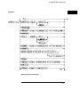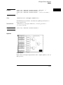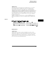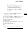
Download Agilent Technologies 1660AS TV Converter Box User Manual

Programmer’s Guide
Publication number 01660-97033
Second edition, January 2000
For Safety information, Warranties, and Regulatory
information, see the pages behind the index
 Copyright Agilent Technologies 1992-2000
All Rights Reserved
Agilent Technologies
1660A/AS-Series Logic
Analyzers
ii
In This Book
This programmer’s guide contains general
information, mainframe level commands,
logic analyzer commands, oscilloscope
module commands, and programming
examples for programming the
1660-series logic analyzers. This guide
focuses on how to program the
instrument over the GPIB and the
RS-232C interfaces.
Instruments covered by the
1660-Series Programmer’s Guide
The 1660-series logic analyzers are
available with or without oscilloscope
measurement capabilities. The
1660A-series logic analyzers contain only
a logic analyzer. The 1660AS-series logic
analyzers contain both a logic analyzer
and a digitizing oscilloscope.
What is in the 1660-Series
Programmer’s Guide?
The 1660-Series Programmer’s Guide
is organized in five parts.
Part 1 Part 1 consists of chapters 1
through 7 and contains general
information about programming basics,
GPIB and RS-232C interface
requirements, documentation
conventions, status reporting , and error
messages.
1
Introduction to Programming
2
Programming Over GPIB
3
Programming Over RS-232C
4
Programming and
Documentation Conventions
5
Message Communication
and System Functions
6
Status Reporting
7
Error Message
8
Common Commands
9
Mainframe Commands
10
SYSTem Subsystem
11
MMEMory Subsystem
12
INTermodule Subsystem
13
MACHine Subsystem
14
WLISt Subsystem
iii
If you are already familiar with IEEE 488.2 programming and GPIB or
RS-232C, you may want to just scan these chapters. If you are new to
programmiung the system, you should read part 1.
Chapter 1 is divided into two sections. The first section, "Talking to the
Instrument," concentrates on program syntax, and the second section,
"Receiving Information from the Instrument," discusses how to send queries
and how to retrieve query results from the instrument.
Read either chapter 2, "Programming Over GPIB," or chapter 3,
"Programming Over RS-232C" for information concerning the physical
connection between the 1660-series logic analyzer and your controller.
Chapter 4, "Programming and Documentation Conventions," gives an
overview of all instructions and also explains the notation conventions used
in the syntax definitions and examples.
Chapter 5, "Message Communication and System Functions," provides an
overview of the operation of instruments that operate in compliance with the
IEEE 488.2 standard.
Chapter 6 explains status reporting and how it can be used to monitor the
flow of your programs and measurement process.
Chapter 7 contains error message descriptions.
Part 2 Part 2, chapters 8 through 12, explain each command in the
command set for the mainframe. These chapters are organized in
subsystems with each subsystem representing a front-panel menu.
The commands explained in this part give you access to common commands,
mainframe commands, system level commands, disk commands, and
intermodule measurement commands. This part is designed to provide a
concise description of each command.
Part 3 Part 3, chapters 13 through 25 explain each command in the
subsystem command set for the logic analyzer. Chapter 26 contains
information on the SYSTem:DATA and SYSTem:SETup commands for
the logic analyzer.
The commands explained in this part give you access to all the commands
used to operate the logic analyzer portion of the 1660-series system. This
part is designed to provide a concise description of each command.
Part 4 Part 4, chapters 27 through 35 explain each command in the
subsystem command set for the oscilloscope.
iv
The commands explained in this part give
you access to all the commands used to
operate the oscilloscope portion of the
1660-series system. This part is designed
to provide a concise description of each
command.
Part 5 Part 5, chapter 36 contains
program examples of actual tasks that
show you how to get started in
programming the 1660-series logic
analyzers. The complexity of your
programs and the tasks they accomplish
are limited only by your imagination.
These examples are written in HP BASIC
6.2; however, the program concepts can
be used in any other popular
programming language that allows
communications over GPIB or RS-232
buses.
15
SFORmat Subsystem
16
STRigger (STRace) Subsystem
17
SLISt Subsystem
18
SWAVeform Subsystem
19
SCHart Subsystem
20
COMPare Subsystem
21
TFORmat Subsystem
22
TRIGger {TRACe} Subsystem
23
TWAVeform Subsystem
24
TLISt Subsystem
25
SYMbol Subsystem
26
DATA and SETup Commands
27
Oscilloscope Root Level
Commands
28
ACQuire Subsystem
v
vi
29
CHANnel Subsystem
30
DISPlay Subsystem
31
MARKer Subsystem
32
MEASure Subsystem
33
TIMebase Subsystem
34
TRIGger Subsystem
35
WAVeform Subsystem
36
Programming Examples
Index
vii
viii
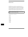
Contents
Part 1 General Information
1 Introduction to Programming
Talking to the Instrument 1–3
Initialization 1–4
Instruction Syntax 1–5
Output Command 1–5
Device Address 1–6
Instructions 1–6
Instruction Terminator 1–7
Header Types 1–8
Duplicate Keywords 1–9
Query Usage 1–10
Program Header Options 1–11
Parameter Data Types 1–12
Selecting Multiple Subsystems 1–14
Receiving Information from the Instrument 1–15
Response Header Options 1–16
Response Data Formats 1–17
String Variables 1–18
Numeric Base 1–19
Numeric Variables 1–19
Definite-Length Block Response Data 1–20
Multiple Queries 1–21
Instrument Status 1–22
2 Programming Over GPIB
Interface Capabilities 2–3
Command and Data Concepts 2–3
Addressing 2–3
Communicating Over the GPIB Bus (HP 9000 Series 200/300 Controller) 2–4
Local, Remote, and Local Lockout 2–5
Bus Commands 2–6
Contents–1
Contents
3 Programming Over RS-232C
Interface Operation 3–3
RS-232C Cables 3–3
Minimum Three-Wire Interface with Software Protocol 3–4
Extended Interface with Hardware Handshake 3–4
Cable Examples 3–6
Configuring the Logic Analzer Interface 3–8
Interface Capabilities 3–9
RS-232C Bus Addressing 3–10
Lockout Command 3–11
4 Programming and Documentation Conventions
Truncation Rule 4–3
Infinity Representation 4–4
Sequential and Overlapped Commands 4–4
Response Generation 4–4
Syntax Diagrams 4–4
Notation Conventions and Definitions 4–5
The Command Tree 4–5
Tree Traversal Rules 4–6
Command Set Organization 4–14
Subsystems 4–15
Program Examples 4–16
5 Message Communication and System Functions
Protocols 5–3
Syntax Diagrams 5–5
Syntax Overview 5–7
6 Status Reporting
Event Status Register 6–4
Service Request Enable Register 6–4
Bit Definitions 6–4
Key Features 6–6
Serial Poll 6–7
Contents–2
Contents
7 Error Messages
Device Dependent Errors 7–3
Command Errors 7–3
Execution Errors 7–4
Internal Errors 7–4
Query Errors 7–5
Part 2 Mainframe Commands
8 Common Commands
*CLS (Clear Status) 8–5
*ESE (Event Status Enable) 8–6
*ESR (Event Status Register) 8–7
*IDN (Identification Number) 8–9
*IST (Individual Status) 8–9
*OPC (Operation Complete) 8–11
*OPT (Option Identification) 8–12
*PRE (Parallel Poll Enable Register Enable) 8–13
*RST (Reset) 8–14
*SRE (Service Request Enable) 8–15
*STB (Status Byte) 8–16
*TRG (Trigger) 8–17
*TST (Test) 8–18
*WAI (Wait) 8–19
9 Mainframe Commands
BEEPer 9–6
CAPability 9–7
CARDcage 9–8
CESE (Combined Event Status Enable) 9–9
CESR (Combined Event Status Register) 9–10
EOI (End Or Identify) 9–11
LER (LCL Event Register) 9–11
LOCKout 9–12
MENU 9–12
Contents–3
Contents
MESE<N> (Module Event Status Enable) 9–14
MESR<N> (Module Event Status Register) 9–16
RMODe 9–18
RTC (Real-time Clock) 9–19
SELect 9–20
SETColor 9–22
STARt 9–23
STOP 9–24
10 SYSTem Subsystem
DATA 10–5
DSP (Display) 10–6
ERRor 10–7
HEADer 10–8
LONGform 10–9
PRINt 10–10
SETup 10–11
11 MMEMory Subsystem
AUToload 11–8
CATalog 11–9
COPY 11–10
DOWNload 11–11
INITialize 11–13
LOAD [:CONFig] 11–14
LOAD :IASSembler 11–15
MSI (Mass Storage Is) 11–16
PACK 11–17
PURGe 11–17
REName 11–18
STORe [:CONFig] 11–19
UPLoad 11–20
VOLume 11–21
Contents–4
Contents
12 INTermodule Subsystem
:INTermodule 12–5
DELete 12–5
HTIMe 12–6
INPort 12–6
INSert 12–7
SKEW<N> 12–8
TREE 12–9
TTIMe 12–10
Part 3 Logic Analyzer Commands
13 MACHine Subsystem
MACHine 13–4
ARM 13–5
ASSign 13–5
LEVelarm 13–6
NAME 13–7
REName 13–8
RESource 13–9
TYPE 13–10
14 WLISt Subsystem
WLISt 14–4
DELay 14–5
INSert 14–6
LINE 14–7
OSTate 14–8
OTIMe 14–8
RANGe 14–9
REMove 14–10
XOTime 14–10
XSTate 14–11
XTIMe 14–11
Contents–5
Contents
15 SFORmat Subsystem
SFORmat 15–6
CLOCk 15–6
LABel 15–7
MASTer 15–9
MODE 15–10
MOPQual 15–11
MQUal 15–12
REMove 15–13
SETHold 15–13
SLAVe 15–15
SOPQual 15–16
SQUal 15–17
THReshold 15–18
16 STRigger (STRace) Subsystem
Qualifier 16–7
STRigger (STRace) 16–9
ACQuisition 16–9
BRANch 16–10
CLEar 16–12
FIND 16–13
RANGe 16–14
SEQuence 16–16
STORe 16–17
TAG 16–18
TAKenbranch 16–19
TCONtrol 16–20
TERM 16–21
TIMER 16–22
TPOSition 16–23
17 SLISt Subsystem
SLISt 17–7
COLumn 17–7
Contents–6
Contents
CLRPattern 17–8
DATA 17–9
LINE 17–9
MMODe 17–10
OPATtern 17–11
OSEarch 17–12
OSTate 17–13
OTAG 17–13
OVERlay 17–14
REMove 17–15
RUNTil 17–15
TAVerage 17–17
TMAXimum 17–17
TMINimum 17–18
VRUNs 17–18
XOTag 17–19
XOTime 17–19
XPATtern 17–20
XSEarch 17–21
XSTate 17–22
XTAG 17–22
18 SWAVeform Subsystem
SWAVeform 18–4
ACCumulate 18–5
ACQuisition 18–5
CENTer 18–6
CLRPattern 18–6
CLRStat 18–7
DELay 18–7
INSert 18–8
RANGe 18–8
REMove 18–9
TAKenbranch 18–9
TPOSition 18–10
Contents–7
Contents
19 SCHart Subsystem
SCHart 19–4
ACCumulate 19–4
HAXis 19–5
VAXis 19–7
20 COMPare Subsystem
COMPare 20–4
CLEar 20–5
CMASk 20–5
COPY 20–6
DATA 20–7
FIND 20–9
LINE 20–10
MENU 20–10
RANGe 20–11
RUNTil 20–12
SET 20–13
21 TFORmat Subsystem
TFORmat 21–4
ACQMode 21–5
LABel 21–6
REMove 21–7
THReshold 21–8
22 TTRigger (TTRace) Subsystem
Qualifier 22–6
TTRigger (TTRace)
ACQuisition 22–9
BRANch 22–9
CLEar 22–12
FIND 22–13
GLEDge 22–14
RANGe 22–15
Contents–8
22–8
Contents
SEQuence 22–17
SPERiod 22–18
TCONtrol 22–19
TERM 22–20
TIMER 22–21
TPOSition 22–22
23 TWAVeform Subsystem
TWAVeform 23–7
ACCumulate 23–7
ACQuisition 23–8
CENTer 23–8
CLRPattern 23–9
CLRStat 23–9
DELay 23–9
INSert 23–10
MMODe 23–11
OCONdition 23–12
OPATtern 23–13
OSEarch 23–14
OTIMe 23–15
RANGe 23–16
REMove 23–16
RUNTil 23–17
SPERiod 23–18
TAVerage 23–19
TMAXimum 23–19
TMINimum 23–20
TPOSition 23–20
VRUNs 23–21
XCONdition 23–22
XOTime 23–22
XPATtern 23–23
XSEarch 23–24
XTIMe 23–25
Contents–9
Contents
24 TLISt Subsystem
TLISt 24–7
COLumn 24–7
CLRPattern 24–8
DATA 24–9
LINE 24–9
MMODe 24–10
OCONdition 24–11
OPATtern 24–11
OSEarch 24–12
OSTate 24–13
OTAG 24–14
REMove 24–14
RUNTil 24–15
TAVerage 24–16
TMAXimum 24–16
TMINimum 24–17
VRUNs 24–17
XCONdition 24–18
XOTag 24–18
XOTime 24–19
XPATtern 24–19
XSEarch 24–20
XSTate 24–21
XTAG 24–22
25 SYMBol Subsystem
SYMBol 25–4
BASE 25–5
PATTern 25–6
RANGe 25–6
REMove 25–7
WIDTh 25–8
Contents–10
Contents
26 DATA and SETup Commands
Data Format 26–3
:SYSTem:DATA 26–4
Section Header Description 26–6
Section Data 26–6
Data Preamble Description 26–6
Acquisition Data Description 26–10
Time Tag Data Description 26–12
Glitch Data Description 26–14
SYSTem:SETup 26–15
RTC_INFO Section Description 26–17
Part 4 Oscilloscope Commands
27 Oscilloscope Root Level Commands
AUToscale 27–3
DIGitize 27–5
28 ACQuire Subsystem
COUNt 28–4
TYPE 28–4
29 CHANnel Subsystem
COUPling 29–4
ECL 29–5
OFFSet 29–6
PROBe 29–7
RANGe 29–8
TTL 29–9
30 DISPlay Subsystem
ACCumulate 30–4
CONNect 30–5
INSert 30–5
Contents–11
Contents
LABel 30–7
MINus 30–8
OVERlay 30–8
PLUS 30–9
REMove 30–9
31 MARKer Subsystem
AVOLt 31–6
ABVolt? 31–7
BVOLt 31–7
CENTer 31–8
MSTats 31–8
OAUTo 31–9
OTIMe 31–10
RUNTil 31–11
SHOW 31–12
TAVerage? 31–12
TMAXimum? 31–13
TMINimum? 31–13
TMODe 31–14
VMODe 31–15
VOTime? 31–16
VRUNs? 31–16
VXTime? 31–17
XAUTo 31–18
XOTime? 31–19
XTIMe 31–19
32 MEASure Subsystem
ALL? 32–5
FALLtime? 32–6
FREQuency? 32–6
NWIDth? 32–7
OVERshoot? 32–7
PERiod? 32–8
PREShoot? 32–8
Contents–12
Contents
PWIDth? 32–9
RISetime? 32–9
SOURce 32–10
VAMPlitude? 32–11
VBASe? 32–11
VMAX? 32–12
VMIN? 32–12
VPP? 32–13
VTOP? 32–13
33 TIMebase Subsystem
DELay 33–4
MODE 33–5
RANGe 33–6
34 TRIGger Subsystem
CONDition 34–5
DELay 34–7
LEVel 34–8
LOGic 34–10
MODE 34–11
PATH 34–12
SLOPe 34–12
SOURce 34–13
35 WAVeform Subsystem
Format for Data Transfer 35–4
Data Conversion 35–6
COUNt? 35–9
DATA? 35–9
FORMat 35–10
POINts? 35–10
PREamble? 35–11
RECord 35–12
SOURce 35–12
Contents–13
Contents
SPERiod? 35–13
TYPE? 35–13
VALid? 35–14
XINCrement? 35–15
XORigin? 35–16
XREFerence? 35–16
YINCrement? 35–17
YORigin? 35–17
YREFerence? 35–18
Part 5 Programming Examples
36 Programming Examples
Making a Timing analyzer measurement 36–3
Making a State analyzer measurement 36–5
Making a State Compare measurement 36–9
Transferring the logic analyzer configuration 36–14
Transferring the logic analyzer acquired data 36–17
Checking for measurement completion 36–21
Sending queries to the logic analyzer 36–22
Getting ASCII Data with PRINt? ALL Query 36–24
Reading the disk with the CATalog? ALL query 36–25
Reading the Disk with the CATalog? Query 36–26
Printing to the disk 36–27
Transferring waveform data in Byte format 36–28
Transferring waveform data in Word format 36–30
Using AUToscale and the MEASure:ALL? Query 36–32
Using Sub-routines in a measurement program 36–33
Contents–14
Part 1
General Information
1
Introduction to Programming
Introduction
This chapter introduces you to the basics of remote programming and
is organized in two sections. The first section, "Talking to the
Instrument," concentrates on initializing the bus, program syntax and
the elements of a syntax instuction. The second section, "Receiving
Information from the Instrument," discusses how queries are sent and
how to retrieve query results from the mainframe instruments.
The programming instructions explained in this book conform to
IEEE Std 488.2-1987, "IEEE Standard Codes, Formats, Protocols, and
Common Commands." These programming instructions provide a
means of remotely controlling the 1660-series logic analyzers. There
are three general categories of use. You can:
• Set up the instrument and start measurements
• Retrieve setup information and measurement results
• Send measurement data to the instrument
The instructions listed in this manual give you access to the
measurements and front panel features of the 1660-series logic
analyzers. The complexity of your programs and the tasks they
accomplish are limited only by your imagination. This programming
reference is designed to provide a concise description of each
instruction.
1–2
Talking to the Instrument
In general, computers acting as controllers communicate with the instrument
by sending and receiving messages over a remote interface, such as GPIB or
RS-232C. Instructions for programming the 1660-series logic analyzers will
normally appear as ASCII character strings embedded inside the output
statements of a "host" language available on your controller. The host
language’s input statements are used to read in responses from the
1660-series logic analyzers.
For example, HP 9000 Series 200/300 BASIC uses the OUTPUT statement for
sending commands and queries to the 1660-series logic analyzers. After a
query is sent, the response can be read in using the ENTER statement. All
programming examples in this manual are presented in HP BASIC.
Example
This Basic statement sends a command that causes the logic analyzer’s
machine 1 to be a state analyzer:
OUTPUT XXX;":MACHINE1:TYPE STATE" <terminator>
Each part of the above statement is explained in this section.
1–3
Introduction to Programming
Initialization
Initialization
To make sure the bus and all appropriate interfaces are in a known state,
begin every program with an initialization statement. BASIC provides a
CLEAR command that clears the interface buffer. If you are using GPIB,
CLEAR will also reset the parser in the logic analyzer. The parser is the
program resident in the logic analyzer that reads the instructions you send to
it from the controller.
After clearing the interface, you could preset the logic analyzer to a known
state by loading a predefined configuration file from the disk.
Refer to your controller manual and programming language reference manual
for information on initializing the interface.
Example
This BASIC statement would load the configuration file "DEFAULT " (if it
exists) into the logic analyzer.
OUTPUT XXX;":MMEMORY:LOAD:CONFIG ’DEFAULT
’"
Refer to chapter 10, "MMEMory Subsystem" for more information on the
LOAD command.
Example Program
10
20
30
40
50
60
70
This program demonstrates the basic command structure used to program
the 1660-series logic analyzers.
CLEAR XXX !Initialize instrument interface
OUTPUT XXX;":SYSTEM:HEADER ON" !Turn headers on
OUTPUT XXX;":SYSTEM:LONGFORM ON"
!Turn longform on
OUTPUT XXX;":MMEM:LOAD:CONFIG ’TEST E’"
!Load configuration file
OUTPUT XXX;":MENU FORMAT,1"
!Select Format menu for machine 1
OUTPUT XXX;":RMODE SINGLE"
!Select run mode
OUTPUT XXX;":START"
!Run the measurement
1–4
Introduction to Programming
Instruction Syntax
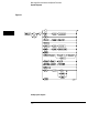
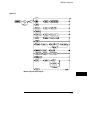
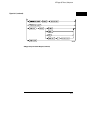
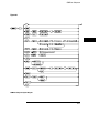
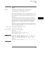
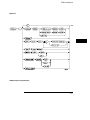
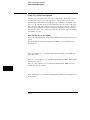
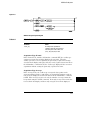
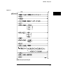
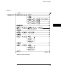
Instruction Syntax
To program the logic analyzer remotely, you must have an understanding of
the command format and structure. The IEEE 488.2 standard governs syntax
rules pertaining to how individual elements, such as headers, separators,
parameters and terminators, may be grouped together to form complete
instructions. Syntax definitions are also given to show how query responses
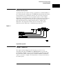
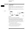
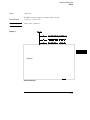
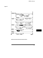
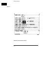
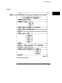
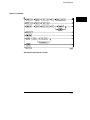
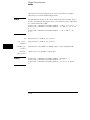
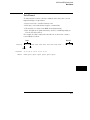
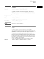
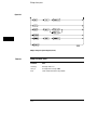
will be formatted. Figure 1-1 shows the three main syntactical parts of a
typical program statement: Output Command, Device Address, and
Instruction. The instruction is further broken down into three parts:
Instruction header, White space, and Instruction parameters.
Figure 1-1
Program Message Syntax
Output Command
The output command depends on the language you choose to use.
Throughout this guide, HP 9000 Series 200/300 BASIC 6.2 is used in the
programming examples. If you use another language, you will need to find
the equivalents of Basic Commands, like OUTPUT, ENTER and CLEAR in
order to convert the examples. The instructions are always shown between
the double quotes.
1–5
Introduction to Programming
Device Address
Device Address
The location where the device address must be specified also depends on the
host language that you are using. In some languages, this could be specified
outside the output command. In BASIC, this is always specified after the
keyword OUTPUT. The examples in this manual use a generic address of
XXX. When writing programs, the number you use will depend on the cable
you use, in addition to the actual address. If you are using an GPIB, see
chapter 2, "Programming over GPIB." If you are using RS-232C, see
chapter 3, "Programming Over RS-232C."
Instructions
Instructions (both commands and queries) normally appear as a string
embedded in a statement of your host language, such as BASIC, Pascal or C.
The only time a parameter is not meant to be expressed as a string is when
the instruction’s syntax definition specifies block data. There are just a few
instructions which use block data.
Instructions are composed of two main parts: the header, which specifies the
command or query to be sent; and the parameters, which provide additional
data needed to clarify the meaning of the instruction. Many queries do not
use any parameters.
Instruction Header
The instruction header is one or more keywords separated by colons (:). The
command tree in figure 4-1 illustrates how all the keywords can be joined
together to form a complete header (see chapter 4, "Programming and
Documentation Conventions").
The example in figure 1-1 shows a command. Queries are indicated by
adding a question mark (?) to the end of the header. Many instructions can
be used as either commands or queries, depending on whether or not you
have included the question mark. The command and query forms of an
instruction usually have different parameters.
1–6
Introduction to Programming
Instruction Terminator
When you look up a query in this programmer’s reference, you’ll find a
paragraph labeled "Returned Format" under the one labeled "Query." The
syntax definition by "Returned format" will always show the instruction
header in square brackets, like [:SYSTem:MENU], which means the text
between the brackets is optional. It is also a quick way to see what the
header looks like.
White Space
White space is used to separate the instruction header from the instruction
parameters. If the instruction does not use any parameters, white space
does not need to be included. White space is defined as one or more spaces.
ASCII defines a space to be a character, represented by a byte, that has a
decimal value of 32. Tabs can be used only if your controller first converts
them to space characters before sending the string to the instrument.
Instruction Parameters
Instruction parameters are used to clarify the meaning of the command or
query. They provide necessary data, such as: whether a function should be
on or off, which waveform is to be displayed, or which pattern is to be looked
for. Each instruction’s syntax definition shows the parameters, as well as the
range of acceptable values they accept. This chapter’s "Parameter Data
Types" section has all of the general rules about acceptable values.
When there is more than one parameter, they are separated by commas (,).
White space surrounding the commas is optional.
Instruction Terminator
An instruction is executed after the instruction terminator is received. The
terminator is the NL (New Line) character. The NL character is an ASCII
linefeed character (decimal 10).
The NL (New Line) terminator has the same function as an EOS (End Of
String) and EOT (End Of Text) terminator.
1–7
Introduction to Programming
Header Types
Header Types
There are three types of headers: Simple Command, Compound Command,
and Common Command.
Simple Command Header
Simple command headers contain a single keyword. START and STOP are
examples of simple command headers typically used in this logic analyzer.
The syntax is: <function><terminator>
When parameters (indicated by <data>) must be included with the simple
command header, the syntax is: <function><white_space><data>
<terminator>
Example
:RMODE SINGLE<terminator>
Compound Command Header
Compound command headers are a combination of two or more program
keywords. The first keyword selects the subsystem, and the last keyword
selects the function within that subsystem. Sometimes you may need to list
more than one subsystem before being allowed to specify the function. The
keywords within the compound header are separated by colons. For
example, to execute a single function within a subsystem, use the following:
:<subsystem>:<function><white_space><data><terminator>
Example
:SYSTEM:LONGFORM ON
To traverse down one level of a subsystem to execute a subsystem within
that subsystem, use the following:
<subsystem>:<subsystem>:<function><white_space>
<data><terminator>
Example
:MMEMORY:LOAD:CONFIG "FILE
1–8
"
Introduction to Programming
Duplicate Keywords
Common Command Header
Common command headers control IEEE 488.2 functions within the logic
analyzer, such as, clear status. The syntax is:
*<command header><terminator>
No white space or separator is allowed between the asterisk and the
command header. *CLS is an example of a common command header.
Combined Commands in the Same Subsystem
To execute more than one function within the same subsystem, a semicolon
(;) is used to separate the functions:
:<subsystem>:<function><white
space><data>;<function><white space><data><terminator>
Example
:SYSTEM:LONGFORM ON;HEADER ON
Duplicate Keywords
Identical function keywords can be used for more than one subsystem. For
example, the function keyword MMODE may be used to specify the marker
mode in the subsystem for state listing or the timing waveforms:
• :SLIST:MMODE PATTERN - sets the marker mode to pattern in
the state listing.
• :TWAVEFORM:MMODE TIME - sets the marker mode to time in the
timing waveforms.
SLIST and TWAVEFORM are subsystem selectors, and they determine which
marker mode is being modified.
1–9
Introduction to Programming
Query Usage
Query Usage
Logic analyzer instructions that are immediately followed by a question mark
(?) are queries. After receiving a query, the logic analyzer parser places the
response in the output buffer. The output message remains in the buffer
until it is read or until another logic analyzer instruction is issued. When
read, the message is transmitted across the bus to the designated listener
(typically a controller).
Query commands are used to find out how the logic analyzer is currently
configured. They are also used to get results of measurements made by the
logic analyzer.
Example
This instruction places the current full-screen time for machine 1 in the
output buffer.
:MACHINE1:TWAVEFORM:RANGE?
In order to prevent the loss of data in the output buffer, the output buffer
must be read before the next program message is sent. Sending another
command before reading the result of the query will cause the output buffer
to be cleared and the current response to be lost. This will also generate a
"QUERY UNTERMINATED" error in the error queue. For example, when you
send the query :TWAVEFORM:RANGE? you must follow that with an input
statement. In Basic, this is usually done with an ENTER statement.
In Basic, the input statement, ENTER XXX; Range, passes the value across
the bus to the controller and places it in the variable Range.
Additional details on how to use queries is in the next section of this chapter,
"Receiving Information for the Instrument."
1–10
Introduction to Programming
Program Header Options
Program Header Options
Program headers can be sent using any combination of uppercase or
lowercase ASCII characters. Logic analyzer responses, however, are always
returned in uppercase.
Both program command and query headers may be sent in either long form
(complete spelling), short form (abbreviated spelling), or any combination of
long form and short form.
Programs written in long form are easily read and are almost selfdocumenting. The short form syntax conserves the amount of controller
memory needed for program storage and reduces the amount of I/O activity.
The rules for short form syntax are discussed in chapter 4, "Programming and
Documentation Conventions."
Example
Either of the following examples turns on the headers and long form.
Long form:
OUTPUT XXX;":SYSTEM:HEADER ON;LONGFORM ON"
Short form:
OUTPUT XXX;":SYST:HEAD ON;LONG ON"
1–11
Introduction to Programming
Parameter Data Types
Parameter Data Types
There are three main types of data which are used in parameters. They are
numeric, string, and keyword. A fourth type, block data, is used only for a few
instructions: the DATA and SETup instructions in the SYSTem subsystem
(see chapter 10); the CATalog, UPLoad, and DOWNload instructions in the
MMEMory subsystem (see chapter 11). These syntax rules also show how
data may be formatted when sent back from the 1660-series logic analyzers
as a response.
The parameter list always follows the instruction header and is separated
from it by white space. When more than one parameter is used, they are
separated by commas. You are allowed to include one or more white spaces
around the commas, but it is not mandatory.
Numeric data
For numeric data, you have the option of using exponential notation or using
suffixes to indicate which unit is being used. However, exponential notation
is only applicable to the decimal number base. Tables 5-1 and 5-2 in chapter
5, "Message Communications and System Functions," list all available
suffixes. Do not combine an exponent with a unit.
Example
The following numbers are all equal:
28 = 0.28E2 = 280E-1 = 28000m = 0.028K.
The base of a number is shown with a prefix. The available bases are binary
(#B), octal (#Q), hexadecimal (#H) and decimal (default).
Example
The following numbers are all equal:
#B11100 = #Q34 = #H1C = 28
You may not specify a base in conjunction with either exponents or unit
suffixes. Additionally, negative numbers must be expressed in decimal.
1–12
Introduction to Programming
Parameter Data Types
When a syntax definition specifies that a number is an integer, that means
that the number should be whole. Any fractional part would be ignored,
truncating the number. Numeric parameters that accept fractional values are
called real numbers.
All numbers are expected to be strings of ASCII characters. Thus, when
sending the number 9, you send a byte representing the ASCII code for the
character "9" (which is 57, or 0011 1001 in binary). A three-digit number,
like 102, will take up three bytes (ASCII codes 49, 48 and 50). This is taken
care of automatically when you include the entire instruction in a string.
String data
String data may be delimited with either single (’) or double (") quotes.
String parameters representing labels are case-sensitive. For instance, the
labels "Bus A" and "bus a" are unique and should not be used
indiscriminately. Also pay attention to the presence of spaces, because they
act as legal characters just like any other. So, the labels "In" and " In" are
also two different labels.
Keyword data
In many cases a parameter must be a keyword. The available keywords are
always included with the instruction’s syntax definition. When sending
commands, either the longform or shortform (if one exists) may be used.
Uppercase and lowercase letters may be mixed freely. When receiving
responses, upper-case letters will be used exclusively. The use of longform
or shortform in a response depends on the setting you last specified via the
SYSTem:LONGform command (see chapter 10).
1–13
Introduction to Programming
Selecting Multiple Subsystems
Selecting Multiple Subsystems
You can send multiple program commands and program queries for different
subsystems on the same line by separating each command with a semicolon.
The colon following the semicolon enables you to enter a new subsystem.
<instruction header><data>;:<instruction header><data>
<terminator>
Multiple commands may be any combination of simple, compound and
common commands.
Example
:MACHINE1:ASSIGN2;:SYSTEM:HEADERS ON
1–14
Receiving Information from the Instrument
After receiving a query (logic analyzer instruction followed by a question
mark), the logic analyzer interrogates the requested function and places the
answer in its output queue. The answer remains in the output queue until it
is read, or, until another command is issued. When read, the message is
transmitted across the bus to the designated listener (typically a controller).
The input statement for receiving a response message from an logic
analyzer’s output queue usually has two parameters: the device address and
a format specification for handling the response message.
All results for queries sent in a program message must be read before another
program message is sent. For example, when you send the query
:MACHINE1:ASSIGN?, you must follow that query with an input statement.
In Basic, this is usually done with an ENTER statement.
The format for handling the response messages is dependent on both the
controller and the programming language.
Example
To read the result of the query command :SYSTEM:LONGFORM? you can
execute this Basic statement to enter the current setting for the long form
command in the numeric variable Setting.
ENTER XXX; Setting
1–15
Introduction to Programming
Response Header Options
Response Header Options
The format of the returned ASCII string depends on the current settings of
the SYSTEM HEADER and LONGFORM commands. The general format is
<instruction_header><space><data><terminator>
The header identifies the data that follows (the parameters) and is controlled
by issuing a :SYSTEM:HEADER ON/OFF command. If the state of the
header command is OFF, only the data is returned by the query.
The format of the header is controlled by the :SYSTEM:LONGFORM ON/OFF
command. If long form is OFF , the header will be in its short form and the
header will vary in length, depending on the particular query. The separator
between the header and the data always consists of one space.
A command or query may be sent in either long form or short form, or in any
combination of long form and short form. The HEADER and LONGFORM
commands only control the format of the returned data, and, they have no
affect on the way commands are sent.
Refer to chapter 10, "SYSTem Subsystem" for information on turning the
HEADER and LONGFORM commands on and off.
Examples
The following examples show some possible responses for a
:MACHINE1:SFORMAT:THRESHOLD2? query:
with HEADER OFF:
<data><terminator>
with HEADER ON and LONGFORM OFF:
:MACH1:SFOR:THR2 <white_space><data><terminator>
with HEADER ON and LONGFORM ON:
:MACHINE1:SFORMAT:THRESHOLD2 <white_space><data><terminator>
1–16
Introduction to Programming
Response Data Formats
Response Data Formats
Both numbers and strings are returned as a series of ASCII characters, as
described in the following sections. Keywords in the data are returned in the
same format as the header, as specified by the LONGform command. Like
the headers, the keywords will always be in uppercase.
Examples
The following are possible responses to the MACHINE1: TFORMAT: LAB?
’ADDR’
query.
Header on; Longform on
MACHINE1:TFORMAT:LABEL "ADDR
",19,POSITIVE<terminator>
Header on;Longform off
MACH1:TFOR:LAB "ADDR
",19,POS<terminator>
Header off; Longform on
"ADDR
",19,POSITIVE<terminator>
Header off; Longform off
"ADDR
",19,POS<terminator>
Refer to the individual commands in Parts 2 through 4 of this guide for
information on the format (alpha or numeric) of the data returned from each
query.
1–17
Introduction to Programming
String Variables
String Variables
Because there are so many ways to code numbers, the 1660-series logic
analyzers handle almost all data as ASCII strings. Depending on your host
language, you may be able to use other types when reading in responses.
Sometimes it is helpful to use string variables in place of constants to send
instructions to the 1660-series logic analyzers, such as, including the headers
with a query response.
Example
5
10
20
30
40
50
60
99
This example combines variables and constants in order to make it easier to
switch from MACHINE1 to MACHINE2. In BASIC, the & operator is used for
string concatenation.
OUTPUT XXX;":SELECT 1"
!Select the logic analyzer
LET Machine$ = ":MACHINE2"
!Send all instructions to machine 2
OUTPUT XXX; Machine$ & ":TYPE STATE" !Make machine a state analyzer
! Assign all labels to be positive
OUTPUT XXX; Machine$ & ":SFORMAT:LABEL ’CHAN 1’, POS"
OUTPUT XXX; Machine$ & ":SFORMAT:LABEL ’CHAN 2’, POS"
OUTPUT XXX; Machine$ & ":SFORMAT:LABEL ’OUT’, POS"
END
If you want to observe the headers for queries, you must bring the returned
data into a string variable. Reading queries into string variables requires little
attention to formatting.
Example
This command line places the output of the query in the string variable
Result$.
ENTER XXX;Result$
In the language used for this book (HP BASIC 6.2), string variables are casesensitive and must be expressed exactly the same each time they are used.
The output of the logic analyzer may be numeric or character data depending
on what is queried. Refer to the specific commands, in Part 2 of this guide,
for the formats and types of data returned from queries.
1–18
Introduction to Programming
Numeric Base
Example
The following example shows logic analyzer data being returned to a string
variable with headers off:
10
20
30
40
50
60
OUTPUT XXX;":SYSTEM:HEADER OFF"
DIM Rang$[30]
OUTPUT XXX;":MACHINE1:TWAVEFORM:RANGE?"
ENTER XXX;Rang$
PRINT Rang$
END
After running this program, the controller displays: +1.00000E-05
Numeric Base
Most numeric data will be returned in the same base as shown onscreen.
When the prefix #B precedes the returned data, the value is in the binary
base. Likewise, #Q is the octal base and #H is the hexadecimal base. If no
prefix precedes the returned numeric data, then the value is in the decimal
base.
Numeric Variables
If your host language can convert from ASCII to a numeric format, then you
can use numeric variables. Turning off the response headers will help you
avoid accidently trying to convert the header into a number.
Example
The following example shows logic analyzer data being returned to a numeric
variable.
10
20
30
40
50
OUTPUT XXX;":SYSTEM:HEADER OFF"
OUTPUT XXX;":MACHINE1:TWAVEFORM:RANGE?"
ENTER XXX;Rang
PRINT Rang
END
1–19
Introduction to Programming
Definite-Length Block Response Data
This time the format of the number (such as, whether or not exponential
notation is used) is dependant upon your host language. In Basic, the output
will look like: 1.E-5
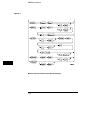
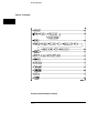
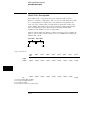
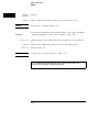
Definite-Length Block Response Data
Definite-length block response data, also refered to as block data, allows any
type of device-dependent data to be transmitted over the system interface as
a series of data bytes. Definite-length blick data is particularly useful for
sending large quantities of data, or, for sending 8-bit extended ASCII codes.
The syntax is a pound sign ( # ) followed by a non-zero digit representing the
number of digits in the decimal integer. Following the non zero digit is the
decimal integer that states the number of 8-bit data bytes to follow. This
number is followed by the actual data.
Indefinite-length block data is not supported on the 1660-series logic
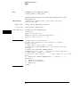
analyzers.
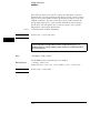
For example, for transmitting 80 bytes of data, the syntax would be:
Figure 1-2
Definite-length Block Response Data
The "8" states the number of digits that follow, and "00000080" states the
number of bytes to be transmitted, which is 80.
1–20
Introduction to Programming
Multiple Queries
Multiple Queries
You can send multiple queries to the logic analyzer within a single program
message, but you must also read them back within a single program message.
This can be accomplished by either reading them back into a string variable
or into multiple numeric variables.
Example
You can read the result of the query :SYSTEM:HEADER?;LONGFORM? into
the string variable Results$ with the command:
ENTER XXX; Results$
When you read the result of multiple queries into string variables, each
response is separated by a semicolon.
Example
The response of the query :SYSTEM:HEADER?:LONGFORM? with HEADER
and LONGFORM turned on is:
:SYSTEM:HEADER 1;:SYSTEM:LONGFORM 1
If you do not need to see the headers when the numeric values are returned,
then you could use numeric variables. When you are receiving numeric data
into numeric variables, the headers should be turned off. Otherwise the
headers may cause misinterpretation of returned data.
Example
The following program message is used to read the query
:SYSTEM:HEADERS?;LONGFORM? into multiple numeric variables:
ENTER XXX; Result1, Result2
1–21
Introduction to Programming
Instrument Status
Instrument Status
Status registers track the current status of the logic analyzer. By checking
the instrument status, you can find out whether an operation has been
completed, whether the instrument is receiving triggers, and more.
Chapter 6, "Status Reporting," explains how to check the status of the
instrument.
1–22
2
Programming Over GPIB
Introduction
This section describes the interface functions and some general
concepts of the GPIB. In general, these functions are defined by IEEE
488.1 (GPIB bus standard). They deal with general bus management
issues, as well as messages which can be sent over the bus as bus
commands.
2–2
Programming Over GPIB
Interface Capabilities
Interface Capabilities
The interface capabilities of the 1660-series logic analyzers, as defined by
IEEE 488.1 are SH1, AH1, T5, TE0, L3, LE0, SR1, RL1, PP0, DC1, DT1, C0,
and E2.
Command and Data Concepts
The GPIB has two modes of operation: command mode and data mode. The
bus is in command mode when the ATN line is true. The command mode is
used to send talk and listen addresses and various bus commands, such as a
group execute trigger (GET). The bus is in the data mode when the ATN line
is false. The data mode is used to convey device-dependent messages across
the bus. These device-dependent messages include all of the instrument
commands and responses found in chapters 8 through 35 of this manual.
Addressing
By using the front-panel I/O and SELECT keys, the GPIB interface can be
placed in either talk only mode, "Printer connected to GPIB," or in addressed
talk/listen mode, "Controller connected to GPIB," (see chapter 16, "The
RS-232/GPIB Menu" in the Agilent Technologies 1660-Series Logic
Analyzer User’s Reference). Talk only mode must be used when you want
the logic analyzer to talk directly to a printer without the aid of a controller.
Addressed talk/listen mode is used when the logic analyzer will operate in
conjunction with a controller. When the logic analyzer is in the addressed
talk/listen mode, the following is true:
• Each device on the GPIB resides at a particular address ranging from 0 to
30.
• The active controller specifies which devices will talk and which will listen.
• An instrument, therefore, may be talk-addressed, listen-addressed, or
unaddressed by the controller.
2–3
Programming Over GPIB
Communicating Over the GPIB Bus (HP 9000 Series 200/300 Controller)
If the controller addresses the instrument to talk, it will remain configured to
talk until it receives:
•
•
•
•
an interface clear message (IFC)
another instrument’s talk address (OTA)
its own listen address (MLA)
a universal untalk (UNT) command.
If the controller addresses the instrument to listen, it will remain configured
to listen until it receives:
• an interface clear message (IFC)
• its own talk address (MTA)
• a universal unlisten (UNL) command.
Communicating Over the GPIB Bus (HP 9000 Series
200/300 Controller)
Because GPIB can address multiple devices through the same interface card,
the device address passed with the program message must include not only
the correct instrument address, but also the correct interface code.
Interface Select Code (Selects the Interface)
Each interface card has its own interface select code. This code is used by
the controller to direct commands and communications to the proper
interface. The default is always "7" for GPIB controllers.
Instrument Address (Selects the Instrument)
Each instrument on the GPIB port must have a unique instrument address
between decimals 0 and 30. The device address passed with the program
message must include not only the correct instrument address, but also the
correct interface select code.
2–4
Programming Over GPIB
Local, Remote, and Local Lockout
Example
For example, if the instrument address is 4 and the interface select code is 7,
the instruction will cause an action in the instrument at device address 704.
DEVICE ADDRESS = (Interface Select Code) X 100 + (Instrument
Address)
Local, Remote, and Local Lockout
The local, remote, and remote with local lockout modes may be used for
various degrees of front-panel control while a program is running. The logic
analyzer will accept and execute bus commands while in local mode, and the
front panel will also be entirely active. If the 1660-series logic analyzer is in
remote mode, the logic analyzer will go from remote to local with any front
panel activity. In remote with local lockout mode, all controls (except the
power switch) are entirely locked out. Local control can only be restored by
the controller.
Hint
Cycling the power will also restore local control, but this will also reset
certain GPIB states. It also resets the logic analyzer to the power-on defaults
and purges any acquired data in the acquisition memory.
The instrument is placed in remote mode by setting the REN (Remote
Enable) bus control line true, and then addressing the instrument to listen.
The instrument can be placed in local lockout mode by sending the local
lockout (LLO) command (see SYSTem:LOCKout in chapter 9, "Mainframe
Commands"). The instrument can be returned to local mode by either
setting the REN line false, or sending the instrument the go to local (GTL)
command.
2–5
Programming Over GPIB
Bus Commands
Bus Commands
The following commands are IEEE 488.1 bus commands (ATN true). IEEE
488.2 defines many of the actions which are taken when these commands are
received by the logic analyzer.
Device Clear
The device clear (DCL) or selected device clear (SDC) commands clear the
input and output buffers, reset the parser, clear any pending commands, and
clear the Request-OPC flag.
Group Execute Trigger (GET)
The group execute trigger command will cause the same action as the
START command for Group Run: the instrument will acquire data for the
active waveform and listing displays.
Interface Clear (IFC)
This command halts all bus activity. This includes unaddressing all listeners
and the talker, disabling serial poll on all devices, and returning control to the
system controller.
2–6
3
Programming Over RS-232C
Introduction
This chapter describes the interface functions and some general
concepts of the RS-232C. The RS-232C interface on this instrument is
Agilent Technologies’ implementation of EIA Recommended Standard
RS-232C, "Interface Between Data Terminal Equipment and Data
Communications Equipment Employing Serial Binary Data
Interchange." With this interface, data is sent one bit at a time, and
characters are not synchronized with preceding or subsequent data
characters. Each character is sent as a complete entity without
relationship to other events.
3–2
Programming Over RS-232C
Interface Operation
Interface Operation
The 1660-series logic analyzers can be programmed with a controller over
RS-232C using either a minimum three-wire or extended hardwire interface.
The operation and exact connections for these interfaces are described in
more detail in the following sections. When you are programming a
1660-series logic analyzer over RS-232C with a controller, you are normally
operating directly between two DTE (Data Terminal Equipment) devices as
compared to operating between a DTE device and a DCE (Data
Communications Equipment) device.
When operating directly between two DTE devices, certain considerations
must be taken into account. For a three-wire operation, XON/XOFF must be
used to handle protocol between the devices. For extended hardwire
operation, protocol may be handled either with XON/XOFF or by
manipulating the CTS and RTS lines of the RS-232C link. For both threewire and extended hardwire operation, the DCD and DSR inputs to the logic
analyzer must remain high for proper operation.
With extended hardwire operation, a high on the CTS input allows the logic
analyzer to send data, and a low disables the logic analyzer data transmission.
Likewise, a high on the RTS line allows the controller to send data, and a low
signals a request for the controller to disable data transmission. Because
three-wire operation has no control over the CTS input, internal pull-up
resistors in the logic analyzer assure that this line remains high for proper
three-wire operation.
RS-232C Cables
Selecting a cable for the RS-232C interface depends on your specific
application, and, whether you wish to use software or hardware handshake
protocol. The following paragraphs describe which lines of the 1660-series
logic analyzer are used to control the handshake operation of the RS-232C
relative to the system. To locate the proper cable for your application, refer
to the reference manual for your computer or controller. Your computer or
controller manual should describe the exact handshake protocol your
controller can use to operate over the RS-232C bus. Also in this chapter you
will find cable recommendations for hardware handshake.
3–3
Programming Over RS-232C
Minimum Three-Wire Interface with Software Protocol
Minimum Three-Wire Interface with Software Protocol
With a three-wire interface, the software (as compared to interface
hardware) controls the data flow between the logic analyzer and the
controller. The three-wire interface provides no hardware means to control
data flow between the controller and the logic analyzer. Therefore,
XON/OFF protocol is the only means to control this data flow. The
three-wire interface provides a much simpler connection between devices
since you can ignore hardware handshake requirements.
The communications software you are using in your computer/controller must
be capable of using XON/XOFF exclusively in order to use three-wire interface
cables. For example, some communications software packages can use
XON/XOFF but are also dependent on the CTS, and DSR lines being true to
communicate.
The logic analyzer uses the following connections on its RS-232C interface for
three-wire communication:
• Pin 7 SGND (Signal Ground)
• Pin 2 TD (Transmit Data from logic analyzer)
• Pin 3 RD (Receive Data into logic analyzer)
The TD (Transmit Data) line from the logic analyzer must connect to the RD
(Receive Data) line on the controller. Likewise, the RD line from the logic
analyzer must connect to the TD line on the controller. Internal pull-up
resistors in the logic analyzer assure the DCD, DSR, and CTS lines remain
high when you are using a three-wire interface.
Extended Interface with Hardware Handshake
With the extended interface, both the software and the hardware can control
the data flow between the logic analyzer and the controller. This allows you
to have more control of data flow between devices. The logic analyzer uses
the following connections on its RS-232C interface for extended interface
communication:
3–4
Programming Over RS-232C
Extended Interface with Hardware Handshake
• Pin 7 SGND (Signal Ground)
• Pin 2 TD (Transmit Data from logic analyzer)
• Pin 3 RD (Receive Data into logic analyzer)
The additional lines you use depends on your controller’s implementation of
the extended hardwire interface.
• Pin 4 RTS (Request To Send) is an output from the logic analyzer which
can be used to control incoming data flow.
• Pin 5 CTS (Clear To Send) is an input to the logic analyzer which
controls data flow from the logic analyzer.
• Pin 6 DSR (Data Set Ready) is an input to the logic analyzer which
controls data flow from the logic analyzer within two bytes.
• Pin 8 DCD (Data Carrier Detect) is an input to the logic analyzer which
controls data flow from the logic analyzer within two bytes.
• Pin 20 DTR (Data Terminal Ready) is an output from the logic analyzer
which is enabled as long as the logic analyzer is turned on.
The TD (Transmit Data) line from the logic analyzer must connect to the RD
(Receive Data) line on the controller. Likewise, the RD line from the logic
analyzer must connect to the TD line on the controller.
The RTS (Request To Send), is an output from the logic analyzer which can
be used to control incoming data flow. A true on the RTS line allows the
controller to send data and a false signals a request for the controller to
disable data transmission.
The CTS (Clear To Send), DSR (Data Set Ready), and DCD (Data Carrier
Detect) lines are inputs to the logic analyzer, which control data flow from
the logic analyzer. Internal pull-up resistors in the logic analyzer assure the
DCD and DSR lines remain high when they are not connected. If DCD or
DSR are connected to the controller, the controller must keep these lines
along with the CTS line high to enable the logic analyzer to send data to the
controller. A low on any one of these lines will disable the logic analyzer data
transmission. Pulling the CTS line low during data transmission will stop
logic analyzer data transmission immediately. Pulling either the DSR or DCD
line low during data transmission will stop logic analyzer data transmission,
but as many as two additional bytes may be transmitted from the logic
analyzer.
3–5
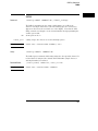
Programming Over RS-232C
Cable Examples
Cable Examples
HP 9000 Series 300
Figure 3-1 is an example of how to connect the 1660-series logic analyzer to
the HP 98628A Interface card of an HP 9000 series 300 controller. For more
information on cabling, refer to the reference manual for your specific
controller.
Because this example does not have the correct connections for hardware
handshake, you must use the XON/XOFF protocol when connecting the logic
analyzer.
Figure 3-1
Cable Example
HP Vectra Personal Computers and Compatibles
Figures 3-2 through 3-4 give examples of three cables that will work for the
extended interface with hardware handshake. Keep in mind that these
cables should work if your computer’s serial interface supports the four
common RS-232C handshake signals as defined by the RS-232C standard.
The four common handshake signals are Data Carrier Detect (DCD), Data
Terminal Ready (DTR), Clear to Send (CTS), and Ready to Send (RTS).
Figure 3-2 shows the schematic of a 25-pin female to 25-pin male cable. The
following cables support this configuration:
• HP 17255D, DB-25(F) to DB-25(M), 1.2 meter
• HP 17255F, DB-25(F) to DB-25(M), 1.2 meter, shielded.
In addition to the female-to-male cables with this configuration, a
male-to-male cable 1.2 meters in length is also available:
• HP 17255M, DB-25(M) to DB-25(M), 1.2 meter
3–6
Programming Over RS-232C
Cable Examples
Figure 3-2
25-pin (F) to 25-pin (M) Cable
Figure 3-3 shows the schematic of a 25-pin male to 25-pin male cable 5
meters in length. The following cable supports this configuration:
• HP 13242G, DB-25(M) to DB-25(M), 5 meter
Figure 3-3
25-pin (M) to 25-pin (M) Cable
3–7
Programming Over RS-232C
Configuring the Logic Analzer Interface
Figure 3-4 shows the schematic of a 9-pin female to 25-pin male cable. The
following cables support this configuration:
• HP 24542G, DB-9(F) to DB-25(M), 3 meter
• HP 24542H, DB-9(F) to DB-25(M), 3 meter, shielded
• HP 45911-60009, DB-9(F) to DB-25(M), 1.5 meter
Figure 3-4
9-pin (F) to 25-pin (M) Cable
Configuring the Logic Analzer Interface
The RS-232C menu field in the System Configuration Menu allows you access
to the RS-232C Configuration menu where the RS-232C interface is
configured. If you are not familiar with how to configure the RS-232C
interface, refer to the Agilent Technologies 1660-Series Logic Analyzer
User’s Reference.
3–8
Programming Over RS-232C
Interface Capabilities
Interface Capabilities
The baud rate, stopbits, parity, protocol, and databits must be configured
exactly the same for both the controller and the logic analyzer to properly
communicate over the RS-232C bus. The RS-232C interface capabilities of
the 1660-series logic analyzers are listed below:
•
•
•
•
•
Baud Rate: 110, 300, 600, 1200, 2400, 4800, 9600, or 19.2k
Stop Bits: 1, 1.5, or 2
Parity: None, Odd, or Even
Protocol: None or XON/XOFF
Data Bits: 8
Protocol
NONE With a three-wire interface, selecting NONE for the protocol
does not allow the sending or receiving device to control dataflow. No
control over the data flow increases the possibility of missing data or
transferring incomplete data.
With an extended hardwire interface, selecting NONE allows a hardware
handshake to occur. With hardware handshake, the hardware signals control
dataflow.
XON/XOFF XON/XOFF stands for Transmit On/Transmit Off. With this
mode, the receiver (controller or logic analyzer) controls dataflow, and,
can request that the sender (logic analyzer or controller) stop dataflow.
By sending XOFF (ASCII 19) over its transmit data line, the receiver
requests that the sender disables data transmission. A subsequent XON
(ASCII 17) allows the sending device to resume data transmission.
Data Bits
Data bits are the number of bits sent and received per character that
represent the binary code of that character. Characters consist of either 7 or
8 bits, depending on the application. The 1660-series logic analyzer supports
8 bit only.
8 Bit Mode Information is usually stored in bytes (8 bits at a time).
With 8-bit mode, you can send and receive data just as it is stored,
without the need to convert the data.
3–9
Programming Over RS-232C
RS-232C Bus Addressing
The controller and the 1660-series logic analyzer must be in the same bit
mode to properly communicate over the RS-232C. This means that the
controller must have the capability to send and receive 8 bit data.
See Also
For more information on the RS-232C interface, refer to the Agilent
Technologies 1660-Series Logic Analyzer User’s Reference. For
information on RS-232C voltage levels and connector pinouts, refer to the
Agilent Technologies 1660-Series Logic Analyzer Service Guide.
RS-232C Bus Addressing
The RS-232C address you must use is dependent on the computer or
controller you are using to communicate with the logic analyzer.
HP Vectra Personal Computers or compatibles
If you are using an HP Vectra Personal Computer or compatible, it must have
an unused serial port to which you connect the logic analyzer’s RS-232C port.
The proper address for the serial port is dependent on the hardware
configuration of your computer. Additionally, your communications software
must be configured to address the proper serial port. Refer to your computer
and communications software manuals for more information on setting up
your serial port address.
HP 9000 Series 300 Controllers
Each RS-232C interface card for the HP 9000 Series 300 Controller has its
own interface select code. This code is used by the controller for directing
commands and communications to the proper interface by specifying the
correct interface code for the device address.
Generally, the interface select code can be any decimal value between 0 and
31, except for those interface codes which are reserved by the controller for
internal peripherals and other internal interfaces. This value can be selected
through switches on the interface card. For example, if your RS-232C
interface select code is 9, the device address required to communicate over
the RS-232C bus is 9. For more information, refer to the reference manual
for your interface card or controller.
3–10
Programming Over RS-232C
Lockout Command
Lockout Command
To lockout the front-panel controls, use the SYSTem command LOCKout.
When this function is on, all controls (except the power switch) are entirely
locked out. Local control can only be restored by sending the :LOCKout OFF
command.
Hint
Cycling the power will also restore local control, but this will also reset
certain RS-232C states. It also resets the logic analyzer to the power-on
defaults and purges any acquired data in the acquisition memory of all the
installed modules.
See Also
For more information on this command see chapter 10, "System Commands."
3–11
3–12
4
Programming and
Documentation Conventions
Introduction
This chapter covers the programming conventions used in
programming the instrument, as well as the documentation
conventions used in this manual. This chapter also contains a detailed
description of the command tree and command tree traversal.
4–2
Programming and Documentation Conventions
Truncation Rule
Truncation Rule
The truncation rule for the keywords used in headers and parameters is:
• If the longform has four or fewer characters, there is no change in the
shortform. When the longform has more than four characters the
shortform is just the first four characters, unless the fourth character is
a vowel. In that case only the first three characters are used.
There are some commands that do not conform to the truncation rule by design.
These will be noted in their respective description pages.
Some examples of how the truncation rule is applied to various commands
are shown in table 4-1.
Table 4-1
Truncation Examples
Long Form
Short Form
OFF
OFF
DATA
DATA
START
STAR
LONGFORM
LONG
DELAY
DEL
ACCUMULATE
ACC
4–3
Programming and Documentation Conventions
Infinity Representation
Infinity Representation
The representation of infinity is 9.9E+37 for real numbers and 32767 for
integers. This is also the value returned when a measurement cannot be
made.
Sequential and Overlapped Commands
IEEE 488.2 makes the distinction between sequential and overlapped
commands. Sequential commands finish their task before the execution of
the next command starts. Overlapped commands run concurrently; therefore,
the command following an overlapped command may be started before the
overlapped command is completed. The overlapped commands for the
1660-series logic analyzers are STARt and STOP.
Response Generation
IEEE 488.2 defines two times at which query responses may be buffered.
The first is when the query is parsed by the instrument and the second is
when the controller addresses the instrument to talk so that it may read the
response. The 1660-series logic analyzers will buffer responses to a query
when it is parsed.
Syntax Diagrams
At the beginning of each chapter in Parts 2 through 4, "Commands," is a
syntax diagram showing the proper syntax for each command. All characters
contained in a circle or oblong are literals, and must be entered exactly as
shown. Words and phrases contained in rectangles are names of items used
with the command and are described in the accompanying text of each
command. Each line can only be entered from one direction as indicated by
the arrow on the entry line. Any combination of commands and arguments
that can be generated by following the lines in the proper direction is
syntactically correct. An argument is optional if there is a path around it.
When there is a rectangle which contains the word "space," a white space
character must be entered. White space is optional in many other places.
4–4
Programming and Documentation Conventions
Notation Conventions and Definitions
Notation Conventions and Definitions
The following conventions are used in this manual when describing
programming rules and example.
< >
Angular brackets enclose words or characters that are used to symbolize a
program code parameter or a bus command
::=
"is defined as." For example, A ::= B indicates that A can be replaced by B in
any statement containing A.
|
"or." Indicates a choice of one element from a list. For example, A | B
indicates A or B, but not both.
...
An ellipsis (trailing dots) is used to indicate that the preceding element may
be repeated one or more times.
[ ]
Square brackets indicate that the enclosed items are optional.
{ }
When several items are enclosed by braces and separated by vertical bars (|),
one, and only one of these elements must be selected.
XXX
Three Xs after an ENTER or OUTPUT statement represent the device
address required by your controller.
<NL>
Linefeed (ASCII decimal 10).
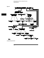
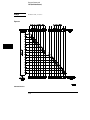
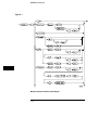
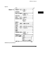
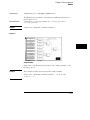
The Command Tree
The command tree (figure 4-1) shows all commands in the 1660-series logic
analyzers and the relationship of the commands to each other. Parameters
are not shown in this figure. The command tree allows you to see what the
1660-series logig analyzer parser expects to receive. All legal headers can be
created by traversing down the tree, adding keywords until the end of a
branch has been reached.
4–5
Programming and Documentation Conventions
Tree Traversal Rules
Command Types
As shown in chapter 1, "Header Types," there are three types of headers.
Each header has a corresponding command type. This section shows how
they relate to the command tree.
System Commands The system commands reside at the top level of
the command tree. These commands are always parsable if they occur at
the beginning of a program message, or are preceded by a colon. START
and STOP are examples of system commands.
Subsystem Commands Subsystem commands are grouped together
under a common node of the tree, such as the MMEMORY commands.
Common Commands Common commands are independent of the tree,
and do not affect the position of the parser within the tree. *CLS and
*RST are examples of common commands.
Tree Traversal Rules
Command headers are created by traversing down the command tree. For
each group of keywords not separated by a branch, one keyword must be
selected. As shown on the tree, branches are always preceded by colons. Do
not add spaces around the colons. The following two rules apply to traversing
the tree:
A leading colon (the first character of a header) or a <terminator> places the
parser at the root of the command tree.
Executing a subsystem command places you in that subsystem until a leading
colon or a <terminator> is found. The parser will stay at the colon above the
keyword where the last header terminated. Any command below that point
can be sent within the current program message without sending the
keywords(s) which appear above them.
4–6
Programming and Documentation Conventions
Tree Traversal Rules
The following examples are written using HP BASIC 6.2 on a HP 9000 Series
200/300 Controller. The quoted string is placed on the bus, followed by a
carriage return and linefeed (CRLF). The three Xs (XXX) shown in this
manual after an ENTER or OUTPUT statement represents the device address
required by your controller.
Example 1
In this example, the colon between SYSTEM and HEADER is necessary since
SYSTEM:HEADER is a compound command. The semicolon between the
HEADER command and the LONGFORM command is the required <program
message unit separator> . The LONGFORM command does not need
SYSTEM preceding it, since the SYSTEM:HEADER command sets the parser
to the SYSTEM node in the tree.
OUTPUT XXX;":SYSTEM:HEADER ON;LONGFORM ON"
Example 2
In the first line of this example, the subsystem selector is implied for the
STORE command in the compound command. The STORE command must
be in the same program message as the INITIALIZE command, since the
<program message terminator> will place the parser back at the root
of the command tree.
A second way to send these commands is by placing MMEMORY: before the
STORE command as shown in the fourth line of this example 2.
OUTPUT XXX;":MMEMORY:INITIALIZE;STORE ’FILE
DESCRIPTION’"
’,’FILE
or
OUTPUT XXX;":MMEMORY:INITIALIZE"
OUTPUT XXX;":MMEMORY:STORE ’FILE
Example 3
’,’FILE DESCRIPTION’"
In this example, the leading colon before SYSTEM tells the parser to go back
to the root of the command tree. The parser can then see the
SYSTEM:PRINT command.
OUTPUT XXX;":MMEM:CATALOG?;:SYSTEM:PRINT ALL"
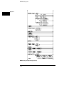
4–7
Programming and Documentation Conventions
Tree Traversal Rules
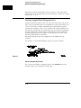
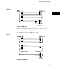
Figure 4-1
1660-Series Logic Analyzer Command Tree
4–8
Programming and Documentation Conventions
Tree Traversal Rules
Figure 4-1 (continued)
1660-Series Logic Analyzer Command Tree (continued)
4–9
Programming and Documentation Conventions
Tree Traversal Rules
Figure 4-1 (continued)
1660-Series Logic Analyzer Command Tree (continued)
4–10
Programming and Documentation Conventions
Tree Traversal Rules
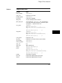
Table 4-2
Alphabetic Command Cross-Reference
Command
ABVOLt
ACCumulate
ACQMode
ACQuisition
ALL
ARM
ASSign
AUToload
AUToscale
AVOLt
BASE
BEEPer
BRANch
BVOLt
CAPability
CARDcage
CATalog
CENTer
CESE
CESR
CLEar
CLOCk
CLRPattern
CLRStat
CMASk
COLumn
CONDition
CONNect
COPY
COUNt
COUPling
DATA
DELay
DELete
DIGitize
DOWNload
Subsystem
MARKer
SCHart, SWAVeform, TWAVeform,
DISPlay
TFORmat
STRigger, SWAVeform, TTRigger,
TWAVeform
MEASure
MACHine
MACHine
MMEMory
MODULE LEVEL
MARKer
SYMBol
Mainframe
STRigger, TTRigger
MARKer
Mainframe
Mainframe
MMEMory
SWAVeform, TWAVeform, MARKer
Mainframe
Mainframe
COMPare, STRigger, TTRigger
SFORmat
SLISt, SWAVeform, TLISt, TWAVeform
SWAVeform, TWAVeform
COMPare
SLISt, TLISt
TRIGger
DISPlay
COMPare, MMEMory
ACQuire, WAVeforml
CHANNel
COMPare, SLISt, SYSTem, TLISt,
WAVeform
SWAVeform, TWAVeform, WLISt,
TIMebase. TRIGger
INTermodule
ROOT
MMEMory
Command
DSP
ECL
EOI
ERRor
FALLtime
FIND
FORMat
FREQuency
GLEDge
HAXis
HEADer
HTIMe
MOPQual
MQUal
MSI
NAME
MACHine
OCONdition
OPATtern
OSEarch
OSTate
OTAG
SLISt, TLISt
OTIMe
OVERlay
PACK
MMEMory
PATTern
PRINt
PURGe
RANGe
REMove
WLISt
REName
REName
RESource
RMODe
RTC
Subsystem
SYSTem
CHANnel
Mainframe
SYSTem
MEASure
COMPare, STRigger, TTRigger
WAVeform
MEASure
TTRigger
SCHart
SYSTem
INTermodule
SFORmat
SFORmat
MMEMory
TLISt, TWAVeform
SLISt, TLISt, TWAVeform
SLISt, TLISt, TWAVeform
SLISt, TLISt, WLISt
TWAVeform, WLISt
SLISt
SYMBol
SYSTem
MMEMory
COMPare, STRigger, SWAVeform,
SYMBol, TTRigger, TWAVeform, WLISt
SFORmat, SLISt, SWAVeform, SYMBol,
TFORmat, TLISt, TWAVeform,
MACHine
MMEMory
MACHine
Mainframe
Mainframe
4–11
Programming and Documentation Conventions
Tree Traversal Rules
Table 4-2 (continued)
Alphabetic Command Cross-Reference (continued)
Command
INITialize
INPort
INSert
LABel
LER
LEVel
LEVelarm
LINE
LOAD
LOCKout
LOGic
LONGform
MASTer
MENU
MESE
MESR
MINus
MMODe
MODE
MOPQual
MQUal
MSI
MSTats
NAME
NWIDth
OAUTo
OCONdition
OFFSet
OPATtern
OSEarch
OSTate
OTAG
OTIMe
OVERlay
OVERshoot
PACK
PATH
PERiod
PATTern
Subsystem
MMEMory
INTermodule
INTermodule, SWAVeform, TWAVeform,
WLISt, DISPlay
SFORmat, TFORmat, DISPlay
Mainframe
TRIGger
MACHine
COMPare, SLISt, TLISt, WLISt
MMEMory
Mainframe
TRIGger
SYSTem
SFORmat
COMPare, Mainframe
Mainframe
Mainframe
DISPlay
SLISt, TLISt, TWAVeform
SFORmat, TIMebase, TRIGger
SFORmat
SFORmat
MMEMory
MARKer
MACHine
MEASure
MARKer
TLISt, TWAVeform
CHANnel
SLISt, TLISt, TWAVeform
SLISt, TLISt, TWAVeform
SLISt, TLISt, WLISt
SLISt, TLISt
TWAVeform, WLISt, MARKer
SLISt, DISPlay
MEASure
MMEMory
TRIGger
MEASure
SYMBol
4–12
Command
PLUS
POINts
PRINt
PREamble
PREShoot
PROBe
PURGe
PWIDth
RANGe
RECord
TREE
TTIMe
TYPE
UPLoad
VAXis
VOLume
VRUNs
WIDTh
XCONdition
XOTag
XOTime
XPATtern
XSEarch
XSTate
XTAG
XTIMe
Subsystem
DISPlay
WAVeform
SYSTem
WAVeform
MEASure
CHANnel
MMEMory
MEASure
COMPare, STRigger, SWAVeform,
SYMBol, TTRigger, TWAVeform, WLISt,
CHANnel, TIMebase
WAVeform
INTermodule
INTermodule
MACHine
MMEMory
SCHart
MMEMory
SLISt, TLISt, TWAVeform
SYMBol
TLISt, TWAVeform
SLISt, TLISt
SLISt, TLISt, TWAVeform, WLISt
SLISt, TLISt, TWAVeform
SLISt, TLISt, TWAVeform
SLISt, TLISt, WLISt
SLISt, TLISt
TWAVeform, WLISt
Programming and Documentation Conventions
Tree Traversal Rules
Table 4-2 (continued)
Alphabetic Command Cross-Reference (continued)
Command
REMove
REName
REName
RESource
RISetime
RMODe
RTC
RUNTil
SELect
SEQuence
SET
SETColor
SETHold
SETup
SHOW
SKEW
SLAVe
SLOPe
SOPQual
SOURce
SPERiod
SQUal
STARt
STOP
STORe
TAG
TAKenbranch
TAVerage
TCONtrol
TERM
THReshold
TIMER
TMAXimum
TMINimum
TMODe
Subsystem
SFORmat, SLISt, SWAVeform, SYMBol,
TFORmat, TLISt, TWAVeform, DISPlay
MACHine
MMEMory
MACHine
MEASure
Mainframe
Mainframe
COMPare, SLISt, TLISt, TWAVeform,
MARKer
Mainframe
STRigger, TTRigger
COMPare
Mainframe
SFORmat
SYSTem
MARKer
INTermodule
SFORmat
TRIGger
SFORmat
MEASure, TRIGger, WAVeform
TTRigger, TWAVeform, WAVeform
SFORmat
Mainframe
Mainframe
MMEMory, STRigger
STRigger
STRigger, SWAVeform
SLISt, TLISt, TWAVeform, MARKer
STRigger, TTRigger
STRigger, TTRigger
SFORmat, TFORmat
STRigger, TTRigger
SLISt, TLISt, TWAVeform, MARKer
SLISt, TLISt, TWAVeform, MARKer
MARKer
Command
TPOSition
TREE
TTIMe
TTL
TYPE
UPLoad
VALid
VAMPlitude
VAXis
VBAse
VOLume
VRUNs
WIDTh
XCONdition
XOTag
XOTime
XPATtern
XSEarch
XSTate
XTAG
XTIMe
Subsystem
STRigger, SWAVeform, TTRigger,
TWAVeform
Intermodule
INTermodule
CHANnel
MACHine, ACQuire, WAVeform
MMEMory
WAVeform
MEASure
SCHart
MEASure
MMEMory
SLISt, TLISt, TWAVeform
SYMBol
TLISt, TWAVeform
SLISt, TLISt
SLISt, TLISt, TWAVeform, WLISt
SLISt, TLISt, TWAVeform
SLISt, TLISt, TWAVeform
SLISt, TLISt, WLISt
SLISt, TLISt
TWAVeform, WLISt
4–13
Programming and Documentation Conventions
Command Set Organization
Table 4-2 (continued)
Alphabetic Command Cross-Reference (continued)
Command
VMAX
VMIN
VMODe
VOLume
VOTime
VPP
VRUNs
VTOP
VXTime
WIDTh
XAUTo
XCONdition
XINCrement
Subsystem
MEASure
MEASure
MARKer
MMEMory
MARKer
MEASure
SLISt, TLISt, TWAVeform, MARKer
MEASure
MARKer
SYMBol
MARKer
TLISt, TWAVeform
WAVeform
XORigin
XOTag
XOTime
XPATtern
XREFerence
WAVeform
SLISt, TLISt
SLISt, TLISt, TWAVeform, WLISt, MARKer
SLISt, TLISt, TWAVeform
WAVeform
XSEarch
SLISt, TLISt, TWAVeform
Command
XSTate
XTAG
XTIMe
YINCrement
YORigin
YREFerence
Subsystem
SLISt, TLISt, WLISt
SLISt, TLISt
TWAVeform, WLISt, MARKer
WAVeform
WAVeform
WAVeform
Command Set Organization
The command set for the 1660-series logic analyzers is divided into 28
separate groups: common commands, mainframe commands, system
commands and 23 sets of subsystem commands. Each of the 28 groups of
commands is described in a seperate chapter in Parts 2 through 4,
"Commands." Each of the chapters contain a brief description of the
subsystem, a set of syntax diagrams for those commands, and finally, the
commands for that subsystem in alphabetical order. The commands are
shown in the long form and short form using upper and lowercase letters. As
an example AUToload indicates that the long form of the command is
AUTOLOAD and the short form of the command is AUT. Each of the
commands contain a description of the command, its arguments, and the
command syntax.
4–14
Programming and Documentation Conventions
Subsystems
Subsystems
There are 23 subsystems in this instrument. In the command tree (figure
4-1) they are shown as branches, with the node above showing the name of
the subsystem. Only one subsystem may be selected at a time. At power on,
the command parser is set to the root of the command tree; therefore, no
subsystem is selected. The 23 subsystems in the 1660-series logic analyzers
are:
•
•
•
•
•
•
•
•
•
•
•
•
•
•
•
•
•
•
•
•
•
•
SYSTem - controls some basic functions of the instrument.
MMEMory - provides access to the internal disk drive.
INTermodule - provides access to the Intermodule bus (IMB).
MACHine - provides access to analyzer functions and subsystems.
WLISt - allows access to the mixed (timing/state) functions.
SFORmat - allows access to the state format functions.
STRigger - allows access to the state trigger functions.
SLISt - allows access to the state listing functions.
SWAVeform - allows access to the state waveforms functions.
SCHart - allows access to the state chart functions.
COMPare - allows access to the compare functions.
TFORmat - allows access to the timing format functions.
TTRigger - allows access to the timing trigger functions.
TWAVeform - allows access to the timing waveforms functions.
TLISt - allows access to the timing listing functions.
SYMBol - allows access to the symbol specification functions.
ACQuire - sets up acquisition conditions for the digitize function.
CHANnel - controls the oscilloscope channel display and vertical axis.
DISPlay - allows data to be displayed.
MARKer - allows access to the oscilloscope’s time and voltage markers.
MEASure - allows automatic parametric measurements.
TIMebase - controls the oscilloscope timebase and horizontal axis.
4–15
Programming and Documentation Conventions
Program Examples
• TRIGger - allows access to the oscilloscope’s trigger functions.
• WAVeform - used to transfer waveform data from the oscilloscope to a
controller.
Program Examples
The program examples in the following chapters and chapter 36,
"Programming Examples," were written on an HP 9000 Series 200/300
controller using the HP BASIC 6.2 language. The programs always assume a
generic address for the 1660-series logic analyzers of XXX.
In the examples, you should pay special attention to the ways in which the
command and/or query can be sent. Keywords can be sent using either the
long form or short form (if one exists for that word). With the exception of
some string parameters, the parser is not case-sensitive. Uppercase and
lowercase letters may be mixed freely. System commands like HEADer and
LONGform allow you to dictate what forms the responses take, but they have
no affect on how you must structure your commands and queries.
Example
The following commands all set the Timing Waveform Delay to 100 ms.
Keywords in long form, numbers using the decimal format.
OUTPUT XXX;":MACHINE1:TWAVEFORM:DELAY .1"
Keywords in short form, numbers using an exponential format.
OUTPUT XXX;":MACH1:TWAV:DEL 1E-1"
Keywords in short form using lowercase letters, numbers using a suffix.
OUTPUT XXX;":mach1:twav:del 100ms"
In these examples, the colon shown as the first character of the command is
optional on the 1660-series logic analyzers. The space between DELay and the
argument is required.
4–16
5
Message Communication and
System Functions
Introduction
This chapter describes the operation of instruments that operate in
compliance with the IEEE 488.2 (syntax) standard. It is intended to
give you enough basic information about the IEEE 488.2 Standard to
successfully program the logic analyzer. You can find additional
detailed information about the IEEE 488.2 Standard in ANSI/IEEE Std
488.2-1987, "IEEE Standard Codes, Formats, Protocols, and
Common Commands."
The 1660-series logic analyzer is designed to be compatible with other
Agilent Technologies IEEE 488.2 compatible instruments.
Instruments that are compatible with IEEE 488.2 must also be
compatible with IEEE 488.1 (GPIB bus standard); however, IEEE
488.1 compatible instruments may or may not conform to the IEEE
488.2 standard. The IEEE 488.2 standard defines the message
exchange protocols by which the instrument and the controller will
communicate. It also defines some common capabilities, which are
found in all IEEE 488.2 instruments. This chapter also contains a few
items which are not specifically defined by IEEE 488.2, but deal with
message communication or system functions.
The syntax and protocol for RS-232C program messages and response
messages for the 1660-series logic analyzer are structured very similar
to those described by 488.2. In most cases, the same structure shown
in this chapter for 488.2 will also work for RS-232C. Because of this,
no additional information has been included for RS-232C.
5–2
Message Communication and System Functions
Protocols
Protocols
The protocols of IEEE 488.2 define the overall scheme used by the controller
and the instrument to communicate. This includes defining when it is
appropriate for devices to talk or listen, and what happens when the protocol
is not followed.
Functional Elements
Before proceeding with the description of the protocol, a few system
components should be understood.
Input Buffer The input buffer of the instrument is the memory area
where commands and queries are stored prior to being parsed and
executed. It allows a controller to send a string of commands to the
instrument which could take some time to execute, and then proceed to
talk to another instrument while the first instrument is parsing and
executing commands.
Output Queue The output queue of the instrument is the memory area
where all output data (<response messages>) are stored until read by
the controller.
Parser The instrument’s parser is the component that interprets the
commands sent to the instrument and decides what actions should be
taken. "Parsing" refers to the action taken by the parser to achieve this
goal. Parsing and executing of commands begins when either the
instrument recognizes a <program message terminator> (defined later in
this chapter) or the input buffer becomes full. If you wish to send a long
sequence of commands to be executed and then talk to another
instrument while they are executing, you should send all the commands
before sending the <program message terminator>.
5–3
Message Communication and System Functions
Protocols
Protocol Overview
The instrument and controller communicate using <program message>s and
<response message>s. These messages serve as the containers into which
sets of program commands or instrument responses are placed. <program
message>s are sent by the controller to the instrument, and <response
message>s are sent from the instrument to the controller in response to a
query message. A <query message> is defined as being a <program
message> which contains one or more queries. The instrument will only talk
when it has received a valid query message, and therefore has something to
say. The controller should only attempt to read a response after sending a
complete query message, but before sending another <program message>.
The basic rule to remember is that the instrument will only talk when
prompted to, and it then expects to talk before being told to do something
else.
Protocol Operation
When the instrument is turned on, the input buffer and output queue are
cleared, and the parser is reset to the root level of the command tree.
The instrument and the controller communicate by exchanging complete
<program message>s and <response message>s. This means that the
controller should always terminate a <program message> before attempting
to read a response. The instrument will terminate <response message>s
except during a hardcopy output.
If a query message is sent, the next message passing over the bus should be
the <response message>. The controller should always read the complete
<response message> associated with a query message before sending another
<program message> to the same instrument.
The instrument allows the controller to send multiple queries in one query
message. This is referred to as sending a "compound query." As will be
noted later in this chapter, multiple queries in a query message are separated
by semicolons. The responses to each of the queries in a compound query
will also be separated by semicolons.
Commands are executed in the order they are received.
5–4
Message Communication and System Functions
Syntax Diagrams
Protocol Exceptions
If an error occurs during the information exchange, the exchange may not be
completed in a normal manner. Some of the protocol exceptions are shown
below.
Command Error A command error will be reported if the instrument
detects a syntax error or an unrecognized command header.
Execution Error An execution error will be reported if a parameter is
found to be out of range, or if the current settings do not allow execution
of a requested command or query.
Device-specific Error A device-specific error will be reported if the
instrument is unable to execute a command for a strictly device
dependent reason.
Query Error A query error will be reported if the proper protocol for
reading a query is not followed. This includes the interrupted and
unterminated conditions described in the following paragraphs.
Syntax Diagrams
The example syntax diagram is in this chapter are similar to the syntax
diagrams in the IEEE 488.2 specification. Commands and queries are sent to
the instrument as a sequence of data bytes. The allowable byte sequence for
each functional element is defined by the syntax diagram that is shown.
The allowable byte sequence can be determined by following a path in the
syntax diagram. The proper path through the syntax diagram is any path
that follows the direction of the arrows. If there is a path around an element,
that element is optional. If there is a path from right to left around one or
more elements, that element or those elements may be repeated as many
times as desired.
5–5
Message Communication and System Functions
Syntax Diagrams
Figure 5-1
Example syntax diagram
5–6
Message Communication and System Functions
Syntax Overview
Syntax Overview
This overview is intended to give a quick glance at the syntax defined by
IEEE 488.2. It will help you understand many of the things about the syntax
you need to know.
IEEE 488.2 defines the blocks used to build messages which are sent to the
instrument. A whole string of commands can therefore be broken up into
individual components.
Figure 5-1 is an example syntax diagram and figure 5-2 shows a breakdown of
an example <program message>. There are a few key items to notice:
• A semicolon separates commands from one another. Each <program
message unit> serves as a container for one command. The <program
message unit>s are separated by a semicolon.
• A <program message> is terminated by a <NL> (new line). The
recognition of the <program message terminator>, or <PMT>, by the
parser serves as a signal for the parser to begin execution of commands.
The <PMT> also affects command tree traversal (Chapter 4,
"Programming and Documentation Conventions").
• Multiple data parameters are separated by a comma.
• The first data parameter is separated from the header with one or more
spaces.
• The header MACHINE1:ASSIGN 2,3 is an example of a compound header.
It places the parser in the machine subsystem until the <NL> is
encountered.
• A colon preceding the command header returns you to the top of the
command tree.
5–7
Message Communication and System Functions
Syntax Overview
Figure 5-2
<program message> Parse Tree
5–8
Message Communication and System Functions
Syntax Overview
Upper/Lower Case Equivalence
Upper and lower case letters are equivalent. The mnemonic SINGLE has
the same semantic meaning as the mnemonic single.
<white space>
<white space> is defined to be one or more characters from the ASCII set of
0 - 32 decimal, excluding 10 decimal (NL). <white space> is used by several
instrument listening components of the syntax. It is usually optional, and can
be used to increase the readability of a program.
Suffix Multiplier The suffix multipliers that the instrument will accept
are shown in table 5-1.
Table 5-1
<suffix mult>
Value
Mnemonic
1E18
EX
1E15
PE
1E12
T
1E9
G
1E6
MA
1E3
K
1E-3
M
1E-6
U
1E-9
N
1E-12
P
1E-15
F
1E-18
A
5–9
Message Communication and System Functions
Syntax Overview
Suffix Unit The suffix units that the instrument will accept are shown
in table 5-2.
Table 5-2
<suffix unit>
Suffix
Referenced Unit
V
Volt
S
Second
5–10
6
Status Reporting
Introduction
Status reporting allows you to use information about the instrument in
your programs, so that you have better control of the measurement
process. For example, you can use status reporting to determine
when a measurement is complete, thus controlling your program, so
that it does not get ahead of the instrument. This chapter describes
the status registers, status bytes and status bits defined by IEEE
488.2 and discusses how they are implemented in the 1660-series
logic analyzers. Also in this chapter is a sample set of steps you use to
perform a serial poll over GPIB.
The status reporting feature available over the bus is the serial poll.
IEEE 488.2 defines data structures, commands, and common bit
definitions. There are also instrument-defined structures and bits.
The bits in the status byte act as summary bits for the data structures
residing behind them. In the case of queues, the summary bit is set if
the queue is not empty. For registers, the summary bit is set if any
enabled bit in the event register is set. The events are enabled via the
corresponding event enable register. Events captured by an event
register remain set until the register is read or cleared. Registers are
read with their associated commands. The *CLS command clears all
event registers and all queues except the output queue. If *CLS is
sent immediately following a <program message terminator>, the
output queue will also be cleared.
6–2
Status Reporting
Figure 6-1
Status Byte Structures and Concepts
6–3
Status Reporting
Event Status Register
Event Status Register
The Event Status Register is an IEEE 488.2 defined register. The bits in this
register are "latched." That is, once an event happens which sets a bit, that
bit will only be cleared if the register is read.
Service Request Enable Register
The Service Request Enable Register is an 8-bit register. Each bit enables
the corresponding bit in the status byte to cause a service request. The sixth
bit does not logically exist and is always returned as a zero. To read and
write to this register, use the *SRE? and *SRE commands.
Bit Definitions
The following mnemonics are used in figure 6-1 and in chapter 8, "Common
Commands:"
MAV - message available
Indicates whether there is a response in the output queue.
ESB - event status bit
Indicates if any of the conditions in the Standard Event Status Register are
set and enabled.
MSS - master summary status
Indicates whether the device has a reason for requesting service. This bit is
returned for the *STB? query.
RQS - request service
Indicates if the device is requesting service. This bit is returned during a
serial poll. RQS will be set to 0 after being read via a serial poll (MSS is not
reset by *STB?).
6–4
Status Reporting
Bit Definitions
MSG - message
Indicates whether there is a message in the message queue (Not
implemented in the 1660-series logic analyzers).
PON - power on
Indicates power has been turned on.
URQ - user request
Always returns a 0 from the 1660-series logic analyzer.
CME - command error
Indicates whether the parser detected an error.
The error numbers and strings for CME, EXE, DDE, and QYE can be read from a
device-defined queue (which is not part of IEEE 488.2) with the query
:SYSTEM:ERROR?.
EXE - execution error
Indicates whether a parameter was out of range, or inconsistent with current
settings.
DDE - device specific error
Indicates whether the device was unable to complete an operation for device
dependent reasons.
QYE - query error
Indicates whether the protocol for queries has been violated.
RQC - request control
Always returns a 0 from the 1660-series logic analyzer.
OPC - operation complete
Indicates whether the device has completed all pending operations. OPC is
controlled by the *OPC common command. Because this command can
appear after any other command, it serves as a general-purpose operation
complete message generator.
6–5
Status Reporting
Key Features
LCL - remote to local
Indicates whether a remote to local transition has occurred.
MSB - module summary bit
Indicates that an enable event in one of the modules Status registers has
occurred.
Key Features
A few of the most important features of Status Reporting are listed in the
following paragraphs.
Operation Complete
The IEEE 488.2 structure provides one technique that can be used to find
out if any operation is finished. The *OPC command, when sent to the
instrument after the operation of interest, will set the OPC bit in the
Standard Event Status Register. If the OPC bit and the RQS bit have been
enabled, a service request will be generated. The commands that affect the
OPC bit are the overlapped commands.
Example
OUTPUT XXX;"*SRE 32 ; *ESE 1"
request
!enables an OPC service
Status Byte
The Status Byte contains the basic status information which is sent over the
bus in a serial poll. If the device is requesting service (RQS set), and the
controller serial-polls the device, the RQS bit is cleared. The MSS (Master
Summary Status) bit (read with *STB?) and other bits of the Status Byte are
not be cleared by reading them. Only the RQS bit is cleared when read.
The Status Byte is cleared with the *CLS common command.
6–6
Status Reporting
Serial Poll
Figure 6-2.
Service Request Enabling
Serial Poll
The 1660-series logic analyzer supports the IEEE 488.1 serial poll feature.
When a serial poll of the instrument is requested, the RQS bit is returned on
bit 6 of the status byte.
6–7
Status Reporting
Serial Poll
Using Serial Poll (GPIB)
This example will show how to use the service request by conducting a serial
poll of all instruments on the GPIB bus. In this example, assume that there
are two instruments on the bus: a Logic Analyzer at address 7 and a printer at
address 1.
The program command for serial poll using HP BASIC 6.2 is Stat =
SPOLL(707). The address 707 is the address of the logic analyzer in the this
example. The command for checking the printer is Stat = SPOLL(701)
because the address of that instrument is 01 on bus address 7. This
command reads the contents of the GPIB Status Register into the variable
called Stat. At that time bit 6 of the variable Stat can be tested to see if it is
set (bit 6 = 1).
The serial poll operation can be conducted in the following manner:
1 Enable interrupts on the bus. This allows the controller to see the
SRQ line.
2 Disable interrupts on the bus.
3 If the SRQ line is high (some instrument is requesting service) then
check the instrument at address 1 to see if bit 6 of its status register is
high.
4 To check whether bit 6 of an instruments status register is high, use
the following BASIC statement•: IF BIT (Stat, 6) THEN
5 If bit 6 of the instrument at address 1 is not high, then check the
instrument at address 7 to see if bit 6 of its status register is high.
6 As soon as the instrument with status bit 6 high is found check the
rest of the status bits to determine what is required.
The SPOLL(707) command causes much more to happen on the bus than
simply reading the register. This command clears the bus automatically,
addresses the talker and listener, sends SPE (serial poll enable) and SPD
(serial poll disable) bus commands, and reads the data. For more
information about serial poll, refer to your controller manual, and
programming language reference manuals.
After the serial poll is completed, the RQS bit in the 1660-series logic
analyzer Status Byte Register will be reset if it was set. Once a bit in the
Status Byte Register is set, it will remain set until the status is cleared with a
*CLS command, or the instrument is reset.
6–8
7
Error Messages
Introduction
This chapter lists the error messages that relate to the 1660-series
logic analyzers.
7–2
Error Messages
Device Dependent Errors
Device Dependent Errors
200
201
202
203
300
Label not found
Pattern string invalid
Qualifier invalid
Data not available
RS-232C error
Command Errors
–100
–101
–110
–111
–120
–121
–123
–129
–130
Command error (unknown command)(generic error)
Invalid character received
Command header error
Header delimiter error
Numeric argument error
Wrong data type (numeric expected)
Numeric overflow
Missing numeric argument
Non numeric argument error (character,string, or block)
–131
–132
–133
–134
–139
–142
–143
–144
Wrong data type (character expected)
Wrong data type (string expected)
Wrong data type (block type #D required)
Data overflow (string or block too long)
Missing non numeric argument
Too many arguments
Argument delimiter error
Invalid message unit delimiter
7–3
Error Messages
Execution Errors
Execution Errors
–200
–201
–202
–203
–211
–212
–221
–222
–232
–240
–241
–242
–243
–244
–245
–246
–247
–248
Can Not Do (generic execution error)
Not executable in Local Mode
Settings lost due to return-to-local or power on
Trigger ignored
Legal command, but settings conflict
Argument out of range
Busy doing something else
Insufficient capability or configuration
Output buffer full or overflow
Mass Memory error (generic)
Mass storage device not present
No media
Bad media
Media full
Directory full
File name not found
Duplicate file name
Media protected
Internal Errors
–300
–301
–302
–303
–310
–311
–312
–313
–320
7–4
Device Failure (generic hardware error)
Interrupt fault
System Error
Time out
RAM error
RAM failure (hardware error)
RAM data loss (software error)
Calibration data loss
ROM error
Error Messages
Query Errors
–321
–322
–330
–340
–350
ROM checksum
Hardware and Firmware incompatible
Power on test failed
Self Test failed
Too Many Errors (Error queue overflow)
Query Errors
–400
–410
–420
–421
–422
–430
Query Error (generic)
Query INTERRUPTED
Query UNTERMINATED
Query received. Indefinite block response in progress
Addressed to Talk, Nothing to Say
Query DEADLOCKED
7–5
7–6
Part 2
Mainframe Commands
8
Common Commands
Introduction
The common commands are defined by the IEEE 488.2 standard.
These commands must be supported by all instruments that comply
with this standard. Refer to figure 8-1 and table 8-1 for the common
commands syntax diagram.
The common commands control some of the basic instrument
functions; such as, instrument identification and reset, how status is
read and cleared, and how commands and queries are received and
processed by the instrument. The common commands are:
•
•
•
•
•
•
•
•
•
•
•
•
•
•
*CLS
*ESE
*ESR
*IDN
*IST
*OPC
*OPT
*PRE
*RST
*SRE
*STB
*TRG
*TST
*WAI
Common commands can be received and processed by the 1660-series
logic analyzers, whether they are sent over the bus as separate
program messages or within other program messages. If an
instrument subsystem has been selected and a common command is
received by the instrument, the logic analyzer will remain in the
selected subsystem.
8–2
Common Commands
Example
If the program message in this example is received by the logic
analyzer, it will initialize the disk and store the file and clear the status
information. This is not be the case if some other type of command is
received within the program message.
":MMEMORY:INITIALIZE;*CLS; STORE ’FILE
Example
’,’DESCRIPTION’"
This program message initializes the disk, selects the module in slot A,
then stores the file. In this example, :MMEMORY must be sent again
in order to reenter the memory subsystem and store the file.
":MMEMORY:INITIALIZE;:SELECT 1;:MMEMORY:STORE ’FILE
’DESCRIPTION’"
’,
Status Registers
Each status register has an associated status enable (mask) register.
By setting the bits in the status enable register you can select the
status information you wish to use. Any status bits that have not been
masked (enabled in the enable register) will not be used to report
status summary information to bits in other status registers.
Refer to chapter 6, "Status Reporting," for a complete discussion of
how to read the status registers and how to use the status information
available from this instrument.
8–3
Common Commands
Figure 8-1
Common Commands Syntax Diagram
8–4
Common Commands
*CLS (Clear Status)
Table 8-1
Common Command Parameter Values
Parameter
Values
mask
An integer, 0 through 255.
pre_mask
An integer, 0 through 65535.
*CLS (Clear Status)
Command
*CLS
The *CLS common command clears all event status registers, queues, and
data structures, including the device defined error queue and status byte. If
the *CLS command immediately follows a <program message terminator>,
the output queue and the MAV (Message Available) bit will be cleared. Refer
to chapter 6, "Status Reporting," for a complete discussion of status.
Example
OUTPUT XXX;"*CLS"
8–5
Common Commands
*ESE (Event Status Enable)
*ESE (Event Status Enable)
Command
*ESE <mask>
The *ESE command sets the Standard Event Status Enable Register bits.
The Standard Event Status Enable Register contains a bit to enable the
status indicators detailed in table 8-2. A 1 in any bit position of the Standard
Event Status Enable Register enables the corresponding status in the
Standard Event Status Enable Register. Refer to Chapter 6, "Status
Reporting" for a complete discussion of status.
<mask>
Example
An integer from 0 to 255
In this example, the *ESE 32 command will enable CME (Command Error),
bit 5 of the Standard Event Status Enable Register. Therefore, when a
command error occurs, the event summary bit (ESB) in the Status Byte
Register will also be set.
OUTPUT XXX;"*ESE 32"
Query
*ESE?
The *ESE query returns the current contents of the enable register.
Returned Format
<mask><NL>
Example
OUTPUT XXX;"*ESE?"
8–6
Common Commands
*ESR (Event Status Register)
Table 8-2
Standard Event Status Enable Register
Bit Position
Bit Weight
Enables
7
128
PON - Power On
6
64
URQ - User Request
5
32
CME - Command Error
4
16
EXE - Execution Error
3
8
DDE - Device Dependent Error
2
4
QYE - Query Error
1
2
RQC - Request Control
0
1
OPC - Operation Complete
*ESR (Event Status Register)
Query
*ESR?
The *ESR query returns the contents of the Standard Event Status Register.
Reading the register clears the Standard Event Status Register.
Returned Format
<status>
Example
<status><NL>
An integer from 0 to 255
If a command error has occurred, and bit 5 of the ESE register is set, the
string variable Esr_event$ will have bit 5 (the CME bit) set.
10 OUTPUT XXX;"*ESE 32
20 OUTPUT XXX;"*ESR?"
30 ENTER XXX; Esr_event$
!Enables bit 5 of the status register
!Queries the status register
!Reads the query buffer
8–7
Common Commands
*ESR (Event Status Register)
Table 8-3 shows the Standard Event Status Register. The table details the
meaning of each bit position in the Standard Event Status Register and the
bit weight. When you read Standard Event Status Register, the value
returned is the total bit weight of all the bits that are high at the time you
read the byte.
Table 8-3
The Standard Event Status Register
Bit Position
Bit Weight
Bit Name
Condition
7
128
PON
0 = register read - not in power up mode
1 = power up
6
64
URQ
0 = user request - not used - always zero
5
32
CME
0 = no command errors
1 = a command eror has been detected
4
16
EXE
0 = no execution errors
1 = an execution error has been detected
3
8
DDE
0 = no device dependent error has been detected
1 = a device dependent error has been detected
2
4
QYE
0 = no query errors
1 = a query error has been detected
1
2
RQC
0 = request control - not used - always zero
0
1
OPC
0 = operation is not complete
1 = operation is complete
8–8
Common Commands
*IDN (Identification Number)
*IDN (Identification Number)
Query
*IDN?
The *IDN? query allows the instrument to identify itself. It returns the string:
"HEWLETT-PACKARD,1660A,0,REV <revision_code>"
An *IDN? query must be the last query in a message. Any queries after the
*IDN? in the program message are ignored.
Returned Format
HEWLETT-PACKARD,1660A,0,REV <revision code>
<revision
code>
Example
Four digit-code in the format XX.XX representing the current ROM revision.
OUTPUT XXX;"*IDN?"
*IST (Individual Status)
Query
*IST?
The *IST query allows the instrument to identify itself during parallel poll by
allowing the controller to read the current state of the IEEE 488.1 defined
"ist" local message in the instrument. The response to this query is
dependent upon the current status of the instrument.
Figure 8-2 shows the *IST data structure.
Returned Format
<id><NL>
<id>
0 or 1
1
Indicates the "ist" local message is false.
0
Indicates the "ist" local message is true.
8–9
Common Commands
*IST (Individual Status)
Example
OUTPUT XXX;"*IST?"
Figure 8-2
*IST Data Structure
8–10
Common Commands
*OPC (Operation Complete)
*OPC (Operation Complete)
Command
*OPC
The *OPC command will cause the instrument to set the operation complete
bit in the Standard Event Status Register when all pending device operations
have finished. The commands which affect this bit are the overlapped
commands. An overlapped command is a command that allows execution of
subsequent commands while the device operations initiated by the
overlapped command are still in progress. The overlapped commands for the
1660-series logic analyzers are STARt and STOP.
Example
OUTPUT XXX;"*OPC"
Query
*OPC?
The *OPC query places an ASCII "1" in the output queue when all pending
device operations have been completed.
Returned Format
1<NL>
Example
OUTPUT XXX;"*OPC?"
8–11
Common Commands
*OPT (Option Identification)
*OPT (Option Identification)
Query
*OPT?
The *OPT query identifies the software installed in the 1660-series logic
analyzer. This query returns nine parameters. The first parameter indicates
whether you are in the system. The next two parameters indicate any
software options installed, and the next parameter indicates whether
intermodule is available for the system. The last five parameters list the
installed software for the modules in slot A through E for an 16500A logic
analysis mainframe. However, the 1660-series logic analyzers have only two
slots (A and B); therefore, only the first and second parameters of the last
five parameters will be relevant. A zero in any of the last eight parameters
indicates that the corresponding software is not currently installed. The
name returned for software options and module software is the same name
that appears in the field in the upper-left corner of the menu for each option
or module.
Returned Format
Example
{SYSTEM},{<option>|0},{<option>|0},{INTERMODULE|0},{<module>|0}
,{<module>|0},{<module>|0},{<module>|0},{<module>|0}<NL>
<option>
Name of software option.
<module>
Name of module software.
OUTPUT XXX;"*OPT?"
8–12
Common Commands
*PRE (Parallel Poll Enable Register Enable)
*PRE (Parallel Poll Enable Register Enable)
Command
*PRE <mask>
The *PRE command sets the parallel poll register enable bits. The Parallel
Poll Enable Register contains a mask value that is ANDed with the bits in the
Status Bit Register to enable an "ist" during a parallel poll. Refer to table 8-4
for the bits in the Parallel Poll Enable Register and for what they mask.
<pre_mask>
Example
An integer from 0 to 65535.
This example will allow the 1660-series logic analyzers to generate an "ist"
when a message is available in the output queue. When a message is
available, the MAV (Message Available) bit in the Status Byte Register will be
high.
Output XXX;"*PRE 16"
Query
*PRE?
The *PRE? query returns the current value of the register.
Returned format
<mask>
Example
<mask><NL>
An integer from 0 through 65535 representing the sum of all bits that are set. .
OUTPUT XXX;"*PRE?"
8–13
Common Commands
*RST (Reset)
Table 8-4
1660-Series Logic Analyzer Parallel Poll Enable Register
Bit Position
Bit Weight
15 -8
Enables
Not used
7
128
Not used
6
64
MSS - Master Summary Status
5
32
ESB - Event Status
4
16
MAV - Message Available
3
8
LCL - Local
2
4
Not used
1
2
Not used
0
1
MSB - Module Summary
*RST (Reset)
The *RST command is not implemented on the 1660-series logic analyzer.
The 1660-series logic analyzer will accept this command, but the command
has no affect on the logic analyzer.
The *RST command is generally used to place the logic analyzer in a
predefined state. Because the 1660-series logic analyzer allows you to store
predefined configuration files for individual modules, or for the entire system,
resetting the logic analyzer can be accomplished by simply loading the
appropriate configuration file. For more information, refer to chapter 11,
"MMEMory Subsystem."
8–14
Common Commands
*SRE (Service Request Enable)
*SRE (Service Request Enable)
Command
*SRE <mask>
The *SRE command sets the Service Request Enable Register bits. The
Service Request Enable Register contains a mask value for the bits to be
enabled in the Status Byte Register. A one in the Service Request Enable
Register will enable the corresponding bit in the Status Byte Register. A zero
will disable the bit. Refer to table 8-5 for the bits in the Service Request
Enable Register and what they mask.
Refer to Chapter 6, "Status Reporting," for a complete discussion of status.
<mask>
Example
An integer from 0 to 255
This example enables a service request to be generated when a message is
available in the output queue. When a message is available, the MAV
(Message Available) bit will be high.
OUTPUT XXX;"*SRE 16"
Query
*SRE?
The *SRE query returns the current value.
Returned Format
<mask>
Example
<mask><NL>
An integer from 0 to 255 representing the sum of all bits that are set.
OUTPUT XXX;"*SRE?"
8–15
Common Commands
*STB (Status Byte)
Table 8-5
1660-Series Logic Analyzer Service Request Enable Register
Bit Position
Bit Weight
15-8
Enables
not used
7
128
not used
6
64
MSS - Master Summary Status (always 0)
5
32
ESB - Event Status
4
16
MAV - Message Available
3
8
LCL- Local
2
4
not used
1
2
not used
0
1
MSB - Module Summary
*STB (Status Byte)
Query
*STB?
The *STB query returns the current value of the instrument’s status byte.
The MSS (Master Summary Status) bit, and, not the RQS (Request Service)
bit is reported on bit 6. The MSS indicates whether or not the device has at
least one reason for requesting service. Refer to table 8-6 for the meaning of
the bits in the status byte.
Refer to Chapter 6, "Status Reporting" for a complete discussion of status.
Returned Format
<value>
Example
<value><NL>
An integer from 0 through 255
OUTPUT XXX;"*STB?"
8–16
Common Commands
*TRG (Trigger)
Table 8-6
The Status Byte Register
Bit Position
Bit Weight
Bit Name
Condition
7
128
6
64
MSS
0 = instrument has no reason for service
1 = instrument is requesting service
5
32
ESB
0 = no event status conditions have occurred
1 = an enabled event status condition has occurred
4
16
MAV
0 = no output messages are ready
1 = an output message is ready
3
8
LCL
0 = a remote-to-local transition has not occurred
1 = a remote-to-local transition has occurred
2
4
1
2
0
1
0 = not Used
not used
not used
MSB
0 = a module or the system has activity to report
1 = no activity to report
0 = False = Low
1 = True = High
*TRG (Trigger)
Command
*TRG
The *TRG command has the same effect as a Group Execute Trigger (GET).
That effect is as if the START command had been sent for intermodule group
run. If no modules are configured in the Intermodule menu, this command
has no effect.
Example
OUTPUT XXX;"*TRG"
8–17
Common Commands
*TST (Test)
*TST (Test)
Query
*TST?
The *TST query returns the results of the power-up self-test. The result of
that test is a 9-bit mapped value which is placed in the output queue. A one
in the corresponding bit means that the test failed and a zero in the
corresponding bit means that the test passed. Refer to table 8-7 for the
meaning of the bits returned by a TST? query.
Returned Format
<result>
<result><NL>
An integer 0 through 511
Example
10 OUTPUT XXX;"*TST?"
20 ENTER XXX;Tst_value
Table 8-7
Bits Returned by *TST? Query (Power-Up Test Results)
Bit Position
Bit Weight
Test
8
256
Disk Test
7
128
not used
6
64
not used
5
32
Front-panel Test
4
16
HIL Test
3
8
Display Test
2
4
Interupt Test
1
2
RAM Test
0
1
ROM Test
8–18
Common Commands
*WAI (Wait)
*WAI (Wait)
Command
*WAI
The *WAI command causes the device to wait until completing all of the
overlapped commands before executing any further commands or queries.
An overlapped command is a command that allows execution of subsequent
commands while the device operations initiated by the overlapped command
are still in progress. Some examples of overlapped commands for the
1660-series logic analyzers are STARt and STOP.
Example:
OUTPUT XXX;"*WAI"
8–19
8–20
9
Mainframe Commands
Introduction
Mainframe commands control the basic operation of the instrument
for the 1660-series logic analyzers. The 1660-series logic analyzers are
similar to a 16500A logic analysis system with either a single logic
analyzer module (1660A) or one logic analyzer and one oscilloscope
module (1660AS) installed.
The main difference in mainframe commands for the 1660-series logic
analyzers is the number of modules. In the 1660 series logic analyzers,
module 0 contains the system level commands, module 1 contains the
logic analyzer level commands, and module 2 contains the
oscilloscope module commands. The command parser in the
1660-series logic analyzers is designed to accept programs written for
the 16500A logic analysis system with a 16550A logic analyzer and/or
oscilloscope modules. The main difference is how you specify the
SELECT command. Remember, the 1660-series logic analyzer is
equivalent only to a mainframe with up to two modules; therefore, if
you specify 3 through 10 for the SELECT command in your program,
the command parser will take no action.
This chapter contains mainframe commands with a syntax example
for each command. Each syntax example contains parameters for the
1600-series logic analyzers only. Refer to figure 9-1 and table 9-1 for
the Mainframe commands syntax diagram. The mainframe commands
are:
•
•
•
•
•
•
•
•
•
9–2
BEEPer
CAPability
CARDcage
CESE
CESR
EOI
LER
LOCKout
MENU
•
•
•
•
•
•
•
•
MESE
MESR
RMODe
RTC
SELect
SETColor
STARt
STOP
Mainframe Commands
Figure 9-1
Mainframe Commands Syntax Diagram
9–3
Mainframe Commands
Figure 9-1 (continued)
Mainframe Commands Syntax Diagram (continued)
9–4
Mainframe Commands
Table 9-1
Mainframe Parameter Values
Parameter
Values
value
An integer from 0 to 65535.
module
An integer 0 through 2 (3 through 10 unused).
menu
An integer.
enable_value
An integer from 0 to 255.
index
An integer from 0 to 5.
day
An integer from 1 through 31
month
An integer from 1 through 12
year
An integer from 1990 through 2089
hour
An integer from 0 through 23
minute
An integer from 0 through 59
second
An integer from 0 through 59
color
An integer from 1 to 7.
hue
An integer from 0 to 100.
sat
An integer from 0 to 100.
lum
An integer from 0 to 100.
9–5
Mainframe Commands
BEEPer
BEEPer
Command
:BEEPer [{ON|1}|{OFF|0}]
The BEEPer command sets the beeper mode, which turns the beeper sound
of the instrument on and off. When BEEPer is sent with no argument, the
beeper will be sounded without affecting the current mode.
Example
OUTPUT XXX;":BEEPER"OUTPUT XXX;":BEEP ON"
Query
:BEEPer?
The BEEPer? query returns the mode currently selected.
Returned Format
[:BEEPer] {1|0}<NL>
Example
OUTPUT XXX;":BEEPER?"
9–6
Mainframe Commands
CAPability
CAPability
Query
:CAPability?
The CAPability query returns the HP-SL (HP System Language) and lower
level capability sets implemented in the device.
Table 9-2 lists the capability sets implemented in the 1660-series logic
analyzers.
Returned Format
[:CAPability]
IEEE488,1987,SH1,AH1,T5,L4,SR1,RL1,PP1,DC1,DT1,C0,E2<NL>
Example
OUTPUT XXX;":CAPABILITY?"
Table 9-2
1660-Series Logic Analyzer Capability Sets
Mnemonic
Capability Name
Implementation
SH
Source Handshake
SH1
AH
Acceptor Handshake
AH1
T
Talker (or TE - Extended Talker)
T5
L
Listener (or LE - Extended Listener)
L4
SR
Service Request
SR1
RL
Remote Local
RL1
PP
Parallel Poll
PP1
DC
Device Clear
DC1
DT
Device Trigger
DT1
C
Any Controller
C0
E
Electrical Characteristic
E2
9–7
Mainframe Commands
CARDcage
CARDcage
Query
:CARDcage?
The CARDcage query returns a series of integers which identify the modules
that are installed in the mainframe. The returned string is in two parts. The
first five two-digit numbers identify the card type. The identification number
for the logic analyzer is 32. The identification number for the oscilloscope is
13. A "-1" in the first part of the string indicates no card is installed in the
slot.
The five single-digit numbers in the second part of the string indicate which
slots have cards installed. The module assignment for the logic analyzer will
always be 1. The second number will contain a 0 unless the oscilloscope
module is installed (1660AS), in which case it will return a 1. The possible
values for the module assignment are 0 and 1 where 0 indicates the module
software is not recognized or not loaded.
Returned Format
<ID>
<assign>
Example
[:CARDcage]
<ID>,<ID>,<ID>,<ID>,<ID><assign>,<assign>,<assign>,
<assign>,<assign><NL>
An integer indicating the card identification number.
An integer indicating the module assignment.
OUTPUT XXX;":CARDCAGE?"
9–8
Mainframe Commands
CESE (Combined Event Status Enable)
CESE (Combined Event Status Enable)
Command
:CESE <value>
The CESE command sets the Combined Event Status Enable register. This
register is the enable register for the CESR register and contains the
combined status of all of the MESE (Module Event Status Enable) registers
of the 1660-series logic analyzer. Table 9-3 lists the bit values for the CESE
register.
<value>
An integer from 0 to 65535
Example
OUTPUT XXX;":CESE 32"
Query
:CESE?
The CESE? query returns the current setting.
Returned Format
[:CESE] <value><NL>
Example
OUTPUT XXX;":CESE?"
Table 9-3
1660-Series Logic Analyzer Combined Event Status Enable Register
Bit
Weight
3 to 15
Enables
not used
2
4
oscilloscope
1
2
logic analyzer
0
1
Intermodule
9–9
Mainframe Commands
CESR (Combined Event Status Register)
CESR (Combined Event Status Register)
Query
:CESR?
The CESR query returns the contents of the Combined Event Status register.
This register contains the combined status of all of the MESRs (Module Event
Status Registers) of the 1660-series logic analyzer. Table 9-4 lists the bit
values for the CESR register.
Returned Format
<value>
[:CESR] <value><NL>
An integer from 0 to 65535
Example
OUTPUT XXX;":CESR?"
Table 9-4
1660-Series Logic Analyzer Combined Event Status Register
Bit
Bit Weight
Bit Name
3 to 15
Condition
0 = not used
2
4
Oscilloscope
0 = No new status
1 = Status to report
1
2
Logic analyzer
0 = No new status
1 = Status to report
0
1
Intermodule
0 = No new status
1 = Status to report
9–10
Mainframe Commands
EOI (End Or Identify)
EOI (End Or Identify)
Command
:EOI {{ON|1}|{OFF|0}}
The EOI command specifies whether or not the last byte of a reply from the
instrument is to be sent with the EOI bus control line set true or not. If EOI
is turned off, the logic analyzer will no longer be sending IEEE 488.2
compliant responses.
Example
OUTPUT XXX;":EOI ON"
Query
:EOI?
The EOI? query returns the current status of EOI.
Returned Format
[:EOI] {1|0}<NL>
Example
OUTPUT XXX;":EOI?"
LER (LCL Event Register)
Query
:LER?
The LER query allows the LCL Event Register to be read. After the LCL
Event Register is read, it is cleared. A one indicates a remote-to-local
transition has taken place. A zero indicates a remote-to-local transition has
not taken place.
Returned Format
[:LER] {0|1}<NL>
Example
OUTPUT XXX;":LER?"
9–11
Mainframe Commands
LOCKout
LOCKout
Command
:LOCKout {{ON|1}|{OFF|0}}
The LOCKout command locks out or restores front panel operation. When
this function is on, all controls (except the power switch) are entirely locked
out.
Example
OUTPUT XXX;":LOCKOUT ON"
Query
:LOCKout?
The LOCKout query returns the current status of the LOCKout command.
Returned Format
[:LOCKout] {0|1}<NL>
Example
OUTPUT XXX;":LOCKOUT?"
MENU
Command
:MENU <module>[,<menu>]
The MENU command puts a menu on the display. The first parameter
specifies the desired module. The optional second parameter specifies the
desired menu in the module (defaults to 0). Table 9-5 lists the parameters
and the menus.
<module>
<menu>
Selects module or system (integer) 0 selects the system, 1 selects the logic
analyzer, and 2 selects the oscilloscope. –2, –1 and 3 to 10 unused)
Selects menu (integer)
9–12
Mainframe Commands
MENU
Example
OUTPUT XXX;":MENU 0,1"
Table 9-5
Menu Parameter Values
Parameters
Menu
0,0
System RS-232/GPIB
0,2
System Disk
0,3
System Utilities
0,4
System Test
1,0
Analyzer Configuration
1,1
Format 1
1,2
Format 2
1,3
Trigger 1
1,4
Trigger 2
1,5
Waveform 1
1,6
Waveform 2
1,7
Listing 1
1,8
Listing 2
1,9
Mixed
1,10
Compare 1
1,11
Compare 2
1,12
Chart 1
1,13
Chart 2
2,0
Channel
2,1
Trigger
2,2
Display
2,3
Auto-measure
2,4
Marker
2,5
Calibration
9–13
Mainframe Commands
MESE<N> (Module Event Status Enable)
Query
:MENU?
The MENU query returns the current menu selection.
Returned Format
[:MENU] <module>,<menu><NL>
Example
OUTPUT XXX;":MENU?"
MESE<N> (Module Event Status Enable)
Command
:MESE<N> <enable_value>
The MESE command sets the Module Event Status Enable register. This
register is the enable register for the MESR register. The <N> index
specifies the module, and the parameter specifies the enable value. For the
1660-series logic analyzer, the <N> index 0, 1, or 2 refers to system, logic
analyzer, or oscilloscope respectively.
<N>
An integer 0 through 2 (3 through 10 unused).
<enable_value>
An integer from 0 through 255
Example
OUTPUT XXX;":MESE1 3"
Query
:MESE<N>?
The query returns the current setting. Tables 9-6, 9-7, and 9-8 list the
Module Event Status Enable register bits, bit weights, and what each bit
masks for the mainframe, logic analyzer, and oscilloscope respectively.
Returned Format
[:MESE<N>] <enable_value><NL>
Example
OUTPUT XXX;":MESE1?"
9–14
Mainframe Commands
MESE<N> (Module Event Status Enable)
Table 9-6
Table 9-7
1660-Series Mainframe (Intermodule) Module Event Status Enable Register
Bit Position
Bit Weight
Enables
7
128
not used
6
84
not used
5
32
not used
4
16
not used
3
8
not used
2
4
not used
1
2
RNT - Intermodule Run Until Satisfied
0
1
MC - Intermodule Measurement Complete
1660-Series Logic Analyzer Module Event Status Enable Register
Bit Position
Bit Weight
Enables
7
128
not used
6
84
not used
5
32
not used
4
16
not used
3
8
Pattern searches failed
2
4
Trigger found
1
2
RNT - Run Until Satisfied
0
1
MC - Measurement Complete
9–15
Mainframe Commands
MESR<N> (Module Event Status Register)
Table 9-8
1660-Series Oscilloscope Module Event Status Enable Register
Bit Position
Bit Weight
Enables
7
128
not used
6
84
not used
5
32
not used
4
16
Number of averages met
3
8
Auto triggered
2
4
Trigger received
1
2
RNT - Run Until Satisfied
0
1
MC - Measurement Complete
MESR<N> (Module Event Status Register)
Query
:MESR<N>?
The MESR query returns the contents of the Module Event Status register.
The <N> index specifies the module. For the 1660 series logic analyzer, the
<N> index 0, 1, or 2 refers to system, logic analyzer, or oscilloscope
respectively.
Refer to table 9-9 for information about the Module Event Status Register
bits and their bit weights for the system, table 9-10 for the logic analyzer, and
table 9-11 for the oscilloscope.
Returned Format
<N>
[:MESR<N>] <enable_value><NL>
An integer 0 through 10 (3 through 10 unused).
<enable_value>
An integer from 0 through 255
Example
OUTPUT XXX;":MESR1?"
9–16
Mainframe Commands
MESR<N> (Module Event Status Register)
Table 9-9
Table 9-10
1660-Series Logic Analyzer Mainframe Module Event Status Register
Bit
Bit Weight
Bit Name
Condition
7
128
0 = not used
6
64
0 = not used
5
32
0 = not used
4
16
0 = not used
3
8
0 = not used
2
4
0 = not used
1
2
RNT
0 = Intermodule Run until not satisfied
1 = Intermodule Run until satisfied
0
1
MC
0 = Intermodule Measurement not satisfied
1 = Intermodule Measurement satisfied
1660-Series Logic Analyzer Module Event Status Register
Bit
Bit Weight
Condition
7
128
0 = not used
6
64
0 = not used
5
32
0 = not used
4
16
0 = not used
3
8
1 = One or more pattern searches failed
0 = Pattern searches did not fail
2
4
1 = Trigger found
0 = Trigger not found
1
2
0 = Run until not satisfied
1 = Run until satisfied
0
1
0 = Measurement not satisfied
1 = Measurement satisfied
9–17
Mainframe Commands
RMODe
Table 9-11
1660-Series Oscilloscope Module Event Status Register
Bit
Bit Weight
Bit Name
Condition
7
128
0 = not used
6
64
0 = not used
5
32
0 = not used
4
16
1 = Number of averages satisfied
0= Number of averages not satisfied
3
8
1 = Auto trigger received
0= Auto trigger not received
2
4
1= Trigger received
0= Trigger not received
1
2
RNT
1 = Run until satisfied
0 = Run until not satisfied
0
1
MC
1 = Measurement complete
0 = Measurement not complete
RMODe
Command
:RMODe {SINGle|REPetitive}
The RMODe command specifies the run mode for the selected module (or
Intermodule). If the selected module is in the intermodule configuration,
then the intermodule run mode will be set by this command.
After specifying the run mode, use the STARt command to start the acquisition.
Example
OUTPUT XXX;":RMODE SINGLE"
9–18
Mainframe Commands
RTC (Real-time Clock)
Query
:RMODe?
The query returns the current setting.
Returned Format
[:RMODe] {SINGle|REPetitive}<NL>
Example
OUTPUT XXX;":RMODE?"
RTC (Real-time Clock)
Command
:RTC {<day>,<month>,<year>,<hour>,<minute>,
<second>|DEFault}
The real-time clock command allows you to set the real-time clock to the
current date and time. The DEFault option sets the real-time clock to 01
January 1990, 12:00:00 (24-hour format).
Example
<day>
integer from 1 to 31
<month>
integer from 1 to 12
<year>
integer from 1990 to 2089
<hour>
integer from 0 to 23
<minute>
integer from 0 to 59
<second>
integer from 0 to 59
This example sets the real-time clock for 1 January 1992, 20:00:00 (8 PM).
OUTPUT XXX;":RTC 1,1,1992,20,0,0"
9–19
Mainframe Commands
SELect
Query
:RTC?
The RTC query returns the real-time clock setting.
Returned Format
[:RTC] <day>,<month>,<year>,<hour>,<minute>,<second>
Example
OUTPUT XXX;":RTC?"
SELect
Command
:SELect <module>
The SELect command selects which module (or system) will have parser
control. SELect defaults to System (0) at power up. The appropriate module
(or system) must be selected before any module (or system) specific
commands can be sent. SELECT 0 selects the System, SELECT 1 selects the
logic analyzer (state and timing), and SELECT 2 selects the oscilloscope
module. Select –2, –1 and, 3 through 10 are accepted but no action will be
taken. When a module is selected, the parser recognizes the module’s
commands and the System/Intermodule commands. When SELECT 0 is
used, only the System/Intermodule commands are recognized by the parser.
Figure 9-2 shows the command tree for the SELect command.
The command parser in the 1660-series logic analyzers is designed to accept
programs written for the 16500A logic analysis system with a 16550A logic
analyzer module; however, if the parameters 3 through 10 are sent, the
1660-series logic analyzer will take no action.
<module>
Example
An integer 0 through 2 (–2, –1, and 3 through 10 unused).
OUTPUT XXX;":SELECT 0"
9–20
Mainframe Commands
SELect
Query
:SELect?
The SELect? query returns the current module selection.
Returned Format
[:SELect] <module><NL>
Example
OUTPUT XXX;":SELECT?"
Figure 9-2
Not Used
Select Command Tree
9–21
Mainframe Commands
SETColor
SETColor
Command
:SETColor {<color>,<hue>,<sat>,<lum>|DEFault}
The SETColor command is used to change one of the selections on the CRT,
or to return to the default screen colors. Four parameters are sent with the
command to change a color:
•
•
•
•
<color>
Color Number (first parameter)
Hue (second parameter)
Saturation (third parameter)
Luminosity (last parameter)
An integer from 1 to 7
<hue>
An integer from 0 to 100.
<sat>
An integer from 0 to 100.
<lum>
An integer from 0 to 100
Color Number 0 cannot be changed.
Example
OUTPUT XXX;":SETCOLOR 3,60,100,60"
OUTPUT XXX;":SETC DEFAULT"
Query
:SETColor? <color>
The SETColor query returns the luminosity values for a specified grey scale.
Returned Format
[:SETColor] <color>,<hue>,<sat>,<lum><NL>
Example
OUTPUT XXX;":SETCOLOR? 3"
9–22
Mainframe Commands
STARt
STARt
Command
:STARt
The STARt command starts the selected module (or Intermodule) running in
the specified run mode (see RMODe). If the specified module is in the
Intermodule configuration, then the Intermodule run will be started.
The STARt command is an overlapped command. An overlapped command is a
command that allows execution of subsequent commands while the device
operations initiated by the overlapped command are still in progress.
Example
OUTPUT XXX;":START"
9–23
Mainframe Commands
STOP
STOP
Command
:STOP
The STOP command stops the selected module (or Intermodule). If the
specified module is in the Intermodule configuration, then the Intermodule
run will be stopped.
The STOP command is an overlapped command. An overlapped command is a
command that allows execution of subsequent commands while the device
operations initiated by the overlapped command are still in progress.
Example
OUTPUT XXX;":STOP"
9–24
10
SYSTem Subsystem
Introduction
SYSTem subsystem commands control functions that are common to
the entire 1660-Series logic analysis system, including formatting
query responses and enabling reading and writing to the advisory line
of the instrument. The command parser in the 1660-series logic
analyzer is designed to accept programs written for the 16500A logic
analysis system with a 16550A logic analyzer module and a 16532A
oscilloscope module.
Refer to figure 10-1 and table 10-1 for the System Subsystem
commands syntax diagram. The SYSTem Subsystem commands are:
•
•
•
•
•
•
•
DATA
DSP
ERRor
HEADer
LONGform
PRINt
SETup
10–2
SYSTem Subsystem
Figure 10-1
System Subsystem Commands Syntax Diagram
10–3
SYSTem Subsystem
System Subsystem Commands Syntax Diagram (Continued)
Table 10-1
SYSTem Parameter Values
Parameter
Values
block_data
Data in IEEE 488.2 format.
string
A string of up to 68 alphanumeric characters.
10–4
SYSTem Subsystem
DATA
DATA
Command
:SYSTem:DATA <block_data>
The DATA command allows you to send and receive acquired data to and
from a controller in block form. This helps saving block data for:
• Reloading to the logic analyzer or oscilloscope
• Processing data later in the logic analyzer or oscilloscope
• Processing data in the controller.
The format and length of block data depends on the instruction being used
and the configuration of the instrument. This chapter describes briefly the
syntax of the Data command and query. Because the mainframe by itself
does not have acquired data, and the capabilities of the DATA command and
query vary for each module, the DATA command and query are described in
detail in the respective modules command section. See chapter 26, "DATA
and SETup Commands" for additional information when using the logic
analyzer, or chapter 35, "WAVeform Subsystem" when using the oscilloscope
module.
Example
OUTPUT XXX;":SYSTEM:DATA" <block_data>
<block_data>
<block_length_
specifier>
<length>
<block_length_specifier><section>
#8<length>
The total length of all sections in byte format (must be represented with 8
digits)
<section>
<section_header><section_data>
<section_
header>
16 bytes, described in the "Section Header Description" section in the
individual modules command section.
<section_data>
The format depends on the type of data
10–5
SYSTem Subsystem
DSP (Display)
Query
:SYSTem:DATA?
The SYSTem:DATA query returns the block data. The data sent by the
SYSTem:DATA query reflects the configuration of the machines when the
last run was performed. Any changes made since then through either
front-panel operations or programming commands do not affect the stored
configuration.
Returned Format
[:SYSTem:DATA] <block_data><NL>
Example
See chapter 36, "Programming Examples" for an example on transferring data.
DSP (Display)
Command
:SYSTem:DSP <string>
The DSP command writes the specified quoted string to a device-dependent
portion of the instrument display.
<string>
Example
A string of up to 68 alphanumeric characters
OUTPUT XXX;":SYSTEM:DSP ’The message goes here’"
10–6
SYSTem Subsystem
ERRor
ERRor
Query
:SYSTem:ERRor? [NUMeric|STRing]
The ERRor query returns the oldest error from the error queue. The optional
parameter determines whether the error string should be returned along with
the error number. If no parameter is received, or if the parameter is
NUMeric, then only the error number is returned. If the value of the
parameter is STRing, then the error should be returned in the following form:
<error_number>,<error_message (string)>
Returned Formats
A complete list of error messages for the 1660A-series logic analyzer is shown
in chapter 7, "Error Messages." If no errors are present in the error queue, a
zero (No Error) is returned.
Numeric:
[:SYSTem:ERRor] <error_number><NL>
String:
[:SYSTem:ERRor] <error_number>,<error_string><NL>
<error_number>
An integer
<error_string>
A string of alphanumeric characters
Examples
Numeric:
10 OUTPUT XXX;":SYSTEM:ERROR?"
20 ENTER XXX;Numeric
String:
50 OUTPUT XXX;":SYST:ERR? STRING"
60 ENTER XXX;String$
10–7
SYSTem Subsystem
HEADer
HEADer
Command
:SYSTem:HEADer {{ON|1}|{OFF|0}}
The HEADer command tells the instrument whether or not to output a
header for query responses. When HEADer is set to ON, query responses will
include the command header.
Example
OUTPUT XXX;":SYSTEM:HEADER ON"
Query
:SYSTem:HEADer?
The HEADer query returns the current state of the HEADer command.
Returned Format
[:SYSTem:HEADer] {1|0}<NL>
Example
OUTPUT XXX;":SYSTEM:HEADER?"
Headers should be turned off when returning values to numeric variables.
10–8
SYSTem Subsystem
LONGform
LONGform
Command
:SYSTem:LONGform {{ON|1}|{OFF|0}}
The LONGform command sets the longform variable, which tells the
instrument how to format query responses. If the LONGform command is set
to OFF, command headers and alpha arguments are sent from the instrument
in the abbreviated form. If the the LONGform command is set to ON, the
whole word will be output. This command has no affect on the input data
messages to the instrument. Headers and arguments may be input in either
the longform or shortform regardless of how the LONGform command is set.
Example
OUTPUT XXX;":SYSTEM:LONGFORM ON"
Query
:SYSTem:LONGform?
The query returns the status of the LONGform command.
Returned Format
[:SYSTem:LONGform] {1|0}<NL>
Example
OUTPUT XXX;":SYSTEM:LONGFORM?"
10–9
SYSTem Subsystem
PRINt
PRINt
Command
:SYSTem:PRINt {ALL|PARTial,<start>,<end>},
DISK,<pathname>
:SYSTem:PRINt SCReen{BTIF|CTIF|PCX|EPS},
DISK,<pathname>
The PRINt command initiates a print of the screen or listing buffer over the
current PRINTER communication interface to the printer or to a file on the
disk. The PRINT SCREEN option allows you to specify a graphics type.
BTIF format is black & white, CTIF and PCX format is color. If a file
extension is not specified, one is appended automatically to the file name.
The PRINT PARTIAL option allows you to specify a START and END state
number.
<pathname>
A string of up to 10 alphanumeric characters for LIF in the following form:
NNNNNNNNNN when the file resides in the present working directory, or a
string of up to 64 alphanumeric characters for DOS in the following forms:
NNNNNNNN.NNN or \NAME_DIR|FILENAME when the file does not reside
in the present working directory.
<start>, <end>
An integer specifying a state number.
Example
This instuctrion prints the screen to the printer:
OUTPUT XXX;":SYSTEM:PRINT SCREEN"
This instruction prints all, to a file named STATE:
OUTPUT 707;":SYSTEM:PRINT ALL, DISK,’STATE’"
This instruction prints partial data to a file named LIST.
OUTPUT 707;":SYSTEM:PRINT PARTIAL,-9,30, DISK,’list’
Query
:SYSTem:PRINt? {SCReen|ALL}
The PRINt query sends the screen or listing buffer data over the current
CONTROLLER communication interface to the controller.
10–10
SYSTem Subsystem
SETup
The print query should NOT be sent with any other command or query on the
same command line. The print query never returns a header. Also, since
response data from a print query may be sent directly to a printer without
modification, the data is not returned in block mode.
Example
OUTPUT 707;":SYSTEM:PRINT? SCREEN"
SETup
Command
:SYStem:SETup <block_data>
The :SYStem:SETup command configures the logic analyzer module as
defined by the block data sent by the controller. This chapter describes
briefly the syntax of the Setup command and query. Because of the
capabilites and importance of the Setup command and query, a complete
chapter is dedicated to it. The dedicated chapter is chapter 26, "DATA and
SETup Commands."
<block_data>
<block_length_
specifier>
<length>
<block_length_specifier><section>
#8<length>
The total length of all sections in byte format (must be represented with 8
digits)
<section>
<section_header><section_data>
<section_
header>
16 bytes, described in the "Section Header Description" section in chapter 26.
<section_data>
Format depends on the type of data
10–11
SYSTem Subsystem
SETup
The total length of a section is 16 (for the section header) plus the length of
the section data. So when calculating the value for <length>, don’t forget
to include the length of the section headers.
Example
OUTPUT XXX USING "#,K";":SYSTEM:SETUP
Query
:SYStem:SETup?
" <block_data>
The SYStem:SETup query returns a block of data that contains the current
configuration to the controller.
Returned Format
[:SYStem:SETup] <block_data><NL>
Example
See "Transferring the logic analyzer configuration" in chapter 27,
"Programming Examples" for an example.
10–12
11
MMEMory Subsystem
Introduction
The MMEMory (mass memory) subsystem commands provide access
to disk drive. The 1600-series logic analyzers support both LIF
(Logical Information Format) and DOS (Disk Operating System)
formats.
The 1660-series logic analyzers have only one disk drive; however,
programs written for the 16500A logic analysis system that contain
the MSI (Mass Storage Is) parameter will be accepted but no action is
taken. Refer to figure 11-1 and table 11-1 for the MMEMory
Subsystem commands syntax diagram. The MMEMory subsystem
commands are:
•
•
•
•
•
•
•
•
•
•
•
•
•
AUToload
CATalog
COPY
DOWNload
INITialize
LOAD
MSI
PACK
PURGe
REName
STORe
UPLoad
VOLume
11–2
MMEMory Subsystem
<msus> refers to the mass storage unit specifier; however, it is not needed for
the 1660-series logic analyzers since they have only one drive. The <msus>
parameter is shown in the command syntax examples as a reminder that for the
the 16500A logic analysis system can be used on the 1660-series logic analyzers.
If you are not going to store information to the configuration disk, or if the disk
you are using contains information you need, it is advisable to write protect
your disk. This will protect the contents of the disk from accidental damage due
to incorrect commands being mistakenly sent.
11–3
MMEMory Subsystem
Figure 11-1
Mmemory Subsystem Commands Syntax Diagram
11–4
MMEMory Subsystem
Figure 11-1
Mmemory Subsystem Commands Syntax Diagram (Continued)
11–5
MMEMory Subsystem
Figure 11-1
Mmemory Subsystem Commands Syntax Diagram (Continued)
11–6
MMEMory Subsystem
Table 11-1
MMEMory Parameter Values
Parameter
Values
auto_file
A string of up to 10 alphanumeric characters for LIF in the
following form: "NNNNNNNNNN"
or
A string of up to 12 alphanumeric characters for DOS in the
following form: "NNNNNNNN.NNN"
msus
Mass Storage Unit specifier (not needed by 1660-series.
16500A <msus> is accepted but no action is taken).
name
A string of up to 10 alphanumeric characters for LIF in the
following form: "NNNNNNNNNN"
or
A string of up to 12 alphanumeric characters for DOS in the
following form: "NNNNNNNN.NNN"
description
A string of up to 32 alphanumeric characters.
type
An integer, refer to table 11-2.
block_data
Data in IEEE 488.2 format.
ia_name
A string of up to 10 alphanumeric characters for LIF in the
following form: "NNNNNNNNNN"
or
A string of up to 12 alphanumeric characters for DOS in the
following form: "NNNNNNNN.NNN"
new_name
A string of up to 10 alphanumeric characters for LIF in the
following form: "NNNNNNNNNN"
or
A string of up to 12 alphanumeric characters for DOS in the
following form: "NNNNNNNN.NNN"
module
An integer, 0 through 2.
11–7
MMEMory Subsystem
AUToload
AUToload
Command
:MMEMory:AUToload {{OFF|0}|{<auto_file>}}[,<msus>]
The AUToload command controls the autoload feature which designates a set
of configuration files to be loaded automatically the next time the instrument
is turned on. The OFF parameter (or 0) disables the autoload feature. A
string parameter may be specified instead to represent the desired autoload
file. If the file is on the current disk, the autoload feature is enabled to the
specified file.
<auto_file>
A string of up to 10 alphanumeric characters for LIF in the following form:
NNNNNNNNNN
or
A string of up to 12 alphanumeric characters for DOS in the following form:
NNNNNNNN.NNN
<msus>
Mass Storage Unit Specifier (not needed by 1660-series. 16500A <msus> is
accepted but no action is taken).
Examples
OUTPUT XXX;":MMEMORY:AUTOLOAD OFF"
OUTPUT XXX;":MMEMORY:AUTOLOAD ’FILE1_A’"
OUTPUT XXX;":MMEMORY:AUTOLOAD ’FILE2 ’,INTERNAL0"
Query
:MMEMory:AUToload?
The AUToload query returns 0 if the autoload feature is disabled. If the
autoload feature is enabled, the query returns a string parameter that
specifies the current autoload file. The appropriate slot designator is
included in the filename and refers to the slot designator A for the logic
analyzer or B for the oscilloscope. If the slot designator is _ (underscore)
the file is for the system.
Returned Format
[:MMEMory:AUToload] {0|<auto_file>},<msus><NL>
11–8
MMEMory Subsystem
CATalog
<auto_file>
A string of up to 10 alphanumeric characters for LIF in the following form:
NNNNNNNNNN
or
A string of up to 12 alphanumeric characters for DOS in the following form:
NNNNNNNN.NNN
Example
OUTPUT XXX;":MMEMORY:AUTOLOAD?"
CATalog
Query
:MMEMory:CATalog? [[All,][<msus>]]
The CATalog query returns the directory of the disk in one of two block data
formats. The directory consists of a 51 character string for each file on the
disk when the ALL option is not used. Each file entry is formatted as follows:
"NNNNNNNNNN TTTTTTT FFFFFFFFFFFFFFFFFFFFFFFFFFFFFFFF"
where N is the filename, T is the file type (see table 11-2), and F is the file
description.
The optional parameter ALL returns the directory of the disk in a
70-character string as follows:
"NNNNNNNNNNNN TTTTTTT FFFFFFFFFFFFFFFFFFFFFFFFFFFFFFFF
DDMMMYY HH:MM:SS"
where N is the filename, T is the file type (see table 11-2), F is the file
description, and, D, M, Y, and HH:MM:SS are the date, month, year, and time
respectively in 24-hour format.
The <msus> is not needed by 1660-series; however, the 16500A <msus> is
accepted but no action is taken.
11–9
MMEMory Subsystem
COPY
<msus>
Returned Format
<block_data>
Example 1
Mass Storage Unit Specifier (not needed by 1660-series. 16500A <msus> is
accepted but no action is taken).
[:MMEMory:CATalog] <block_data>
ASCII block containing <filename> <file_type>
<file_description>
This example is for sending the CATALOG? ALL query:
OUTPUT 707;":MMEMORY:CATALOG? ALL"
Example 2
This example is for sending the CATALOG? query without the ALL option.
Keep in mind if you do not use the ALL option with a DOS disk, each
filename entry will be truncated at 51 characters:
OUTPUT 707;":MMEMORY:CATALOG?"
COPY
Command
:MMEMory:COPY <name>[,<msus>],<new_name>[,<msus>]
The COPY command copies one file to a new file or an entire disk’s contents
to another disk. The two <name> parameters are the filenames. The first
pair of parameters specifies the source file. The second pair specifies the
destination file. An error is generated if the source file doesn’t exist, or if the
destination file already exists.
The <msus> is not needed by 1660-series. 16500A <msus> is accepted but
no action is taken.
11–10
MMEMory Subsystem
DOWNload
<name>
A string of up to 10 alphanumeric characters for LIF in the following form:
NNNNNNNNNN
or
A string of up to 12 alphanumeric characters for DOS in the following form:
NNNNNNNN.NNN
<new_name>
A string of up to 10 alphanumeric characters for LIF in the following form:
NNNNNNNNNN
or
A string of up to 12 alphanumeric characters for DOS in the following form:
NNNNNNNN.NNN
<msus>
Examples
Mass Storage Unit Specifier (not needed by 1660-series. 16500A <msus> is
accepted but no action is taken).
To copy the contents of "FILE1" to "FILE2:
OUTPUT XXX;":MMEMORY:COPY ’FILE1’,’FILE2’"
DOWNload
Command
:MMEMory:DOWNload <name>[,<msus>],<description>,
<type>,<block_data>
The DOWNload command downloads a file to the mass storage device. The
<name> parameter specifies the filename, the <description> parameter
specifies the file descriptor, and the <block_data> contains the contents
of the file to be downloaded.
The <msus> is not needed by 1660-series. 16500A <msus> is accepted but
no action is taken.
Table 11-2 lists the file types for the <type> parameter.
11–11
MMEMory Subsystem
DOWNload
<name>
A string of up to 10 alphanumeric characters for LIF in the following form:
NNNNNNNNNN
or
A string of up to 12 alphanumeric characters for DOS in the following form:
NNNNNNNN.NNN
<msus>
<description>
<type>
<block_data>
Mass Storage Unit Specifier (not needed by 1660-series. 16500A <msus> is
accepted but no action is taken).
A string of up to 32 alphanumeric characters
An integer (see table 11-2)
Contents of file in block data format
Example
OUTPUT XXX;":MMEMORY:DOWNLOAD ’SETUP
QUERY’,-16127,#800000643..."
Table 11-2
’,INTERNAL0,’FILE CREATED FROM SETUP
File Types
File
File Type
1660-Series System Software
–15608
1660-Series ROM Software
–15609
1660-Series System Configuration
–15605
1660-Series Logic Analyzer Configuration
–16095
1660-Series Logic Analyzer Software
–15607
1660-Series Logic Analyzer with Oscilloscope Configuration
–16115
1660-Series Oscilloscope Software
–15606
Autoload File
–15615
Inverse Assembler
–15614
Text Type (LIF from Print to Disk)
–5813
11–12
MMEMory Subsystem
INITialize
INITialize
Command
:MMEMory:INITialize [{LIF|DOS}[,<msus>]]
The INITialize command formats the disk in either LIF (Logical Information
Format) or DOS (Disk Operating System). The <msus> is not needed by
1660-series. 16500A <msus> is accepted but no action is taken. If no
format is specified, then the initialize command will format the disk in the LIF
format.
<msus>
Examples
Mass Storage Unit Specifier (not needed by 1660-series. 16500A <msus> is
accepted but no action is taken).
OUTPUT XXX;":MMEMORY:INITIALIZE DOS"
OUTPUT XXX;":MMEMORY:INITIALIZE LIF,INTERNAL0"
Once executed, the initialize command formats the specified disk, permanently
erasing all existing information from the disk. After that, there is no way to
retrieve the original information.
11–13
MMEMory Subsystem
LOAD [:CONFig]
LOAD [:CONFig]
Command
:MMEMory:LOAD[:CONfig] <name>[,<msus>][,<module>]
The LOAD command loads a configuration file from the disk into the logic
analyzer, oscilloscope, software options, or the system. The <name>
parameter specifies the filename from the disk. The optional <module>
parameter specifies which module(s) to load the file into. The accepted
values are 0 for system, 1 for logic analyzer, and 2 for the oscilloscope. Not
specifying the <module> parameter is equivalent to performing a ’LOAD
ALL’ from the front panel which loads the appropriate file for the system,
logic analyzer, oscilloscope, and any software option.
<name>
A string of up to 10 alphanumeric characters for LIF in the following form:
NNNNNNNNNN
or
A string of up to 12 alphanumeric characters for DOS in the following form:
NNNNNNNN.NNN
<msus>
<module>
Examples
Mass Storage Unit Specifier (not needed by 1660-series. 16500A <msus> is
accepted but no action is taken).
An integer, 0 through 2
OUTPUT XXX;":MMEMORY:LOAD:CONFIG ’FILE ’"
OUTPUT XXX;":MMEMORY:LOAD ’FILE ’,0"
OUTPUT XXX;":MMEM:LOAD:CONFIG ’FILE A’,INTERNAL0,1"
11–14
MMEMory Subsystem
LOAD :IASSembler
LOAD :IASSembler
Command
:MMEMory:LOAD:IASSembler <IA_name>[,<msus>],{1|2}
[,<module>]
This variation of the LOAD command allows inverse assembler files to be
loaded into a module that performs state analysis. The <IA_name>
parameter specifies the inverse assembler filename from the desired
<msus>. The parameter after the optional <msus> specifies which machine
to load the inverse assembler into.
The optional <module> parameter is used to specify which slot the state
analyzer in. 1 refers to the logic analyzer. If this parameter is not specified,
the state analyzer will be selected.
<IA_name>
A string of up to 10 alphanumeric characters for LIF in the following form:
NNNNNNNNNN
or
A string of up to 12 alphanumeric characters for DOS in the following form:
NNNNNNNN.NNN
<msus>
<module>
Examples
Mass Storage Unit Specifier (not needed by 1660-series. 16500A <msus> is
accepted but no action is taken).
An integer, always 1
OUTPUT XXX;":MMEMORY:LOAD:IASSEMBLER ’I68020 IP’,1"
OUTPUT XXX;":MMEM:LOAD:IASS ’I68020 IP’,INTERNAL0,1,2"
11–15
MMEMory Subsystem
MSI (Mass Storage Is)
MSI (Mass Storage Is)
Command
:MMEMory:MSI [<msus>]
The MSI command selects a default mass storage device; however, it is not
needed by 1660-series logic analyzers because they have only one disk drive.
If the 16500A <msus> is sent to the 1660-series logic analyzer, it is accepted
but no action is taken.
<msus>
Mass Storage Unit Specifier (not needed by 1660-series. 16500A <msus> is
accepted but no action is taken).
Examples
OUTPUT XXX;":MMEMORY:MSI"
OUTPUT XXX;":MMEM:MSI INTERNAL0"
Query
:MMEMory:MSI?
The MSI? query returns the current MSI setting. Because the 1660-series
logic analyzers have only one disk drive, Internal0 is always returned.
Returned Format
[:MMEMory:MSI] <msus><NL>
Example
OUTPUT XXX;":MMEMORY:MSI?"
11–16
MMEMory Subsystem
PACK
PACK
Command
:MMEMory:PACK [<msus>]
The PACK command packs the files on the LIF disk the disk in the drive. If a
DOS disk is in the drive when the PACK command is sent, no action is taken.
<msus>
Examples
Mass Storage Unit Specifier (not needed by 1660-series. 16500A <msus> is
accepted but no action is taken).
OUTPUT XXX;":MMEMORY:PACK"
OUTPUT XXX;":MMEM:PACK INTERNAL0"
PURGe
Command
:MMEMory:PURGe <name>[,<msus>]
The PURGe command deletes a file from the disk in the drive. The <name>
parameter specifies the filename to be deleted.
<name>
A string of up to 10 alphanumeric characters for LIF in the following form:
NNNNNNNNNN
or
A string of up to 12 alphanumeric characters for DOS in the following form:
NNNNNNNN.NNN
<msus>
Mass Storage Unit Specifier (not needed by 1660-series. 16500A <msus> is
accepted but no action is taken).
11–17
MMEMory Subsystem
REName
Examples
OUTPUT XXX;":MMEMORY:PURGE ’FILE1’"
OUTPUT XXX;":MMEM:PURG ’FILE1’,INTERNAL0"
Once executed, the purge command permanently erases all the existing
information about the specified file. After that, there is no way to retrieve the
original information.
REName
Command
:MMEMory:REName <name>[,<msus>],<new_name>
The REName command renames a file on the disk in the drive. The <name>
parameter specifies the filename to be changed and the <new_name>
parameter specifies the new filename.
You cannot rename a file to an already existing filename.
<name>
A string of up to 10 alphanumeric characters for LIF in the following form:
NNNNNNNNNN
or
A string of up to 12 alphanumeric characters for DOS in the following form:
NNNNNNNN.NNN
<msus>
<new name>
Mass Storage Unit Specifier (not needed by 1660-series. 16500A <msus> is
accepted but no action is taken).
A string of up to 10 alphanumeric characters for LIF in the following form:
NNNNNNNNNN
or
A string of up to 12 alphanumeric characters for DOS in the following form:
NNNNNNNN.NNN
11–18
MMEMory Subsystem
STORe [:CONFig]
Examples
OUTPUT XXX;":MMEMORY:RENAME ’OLDFILE’,’NEWFILE’"
OUTPUT XXX;":MMEM:REN ’OLDFILE’[,INTERNAL1],’NEWFILE’"
STORe [:CONFig]
Command
:MMEMory:STORe [:CONfig]<name>[,<msus>],
<description>[,<module>]
The STORe command stores module or system configurations onto a disk.
The [:CONFig] specifier is optional and has no effect on the command. The
<name> parameter specifies the file on the disk. The <description>
parameter describes the contents of the file. The optional <module>
parameter allows you to store the configuration for either the system, the
logic analyzer, or the oscilloscope. 2 refers to the oscilloscope, 1 refers to the
logic analyzer, and 0 refers to the system.
If the optional <module> parameter is not specified, the configurations for
the system, logic analyzer, and oscilloscope are stored.
<name>
A string of up to 10 alphanumeric characters for LIF in the following form:
NNNNNNNNNN
or
A string of up to 12 alphanumeric characters for DOS in the following form:
NNNNNNNN.NNN
<msus>
<description>
<module>
Mass Storage Unit Specifier (not needed by 1660-series. 16500A <msus> is
accepted but no action is taken).
A string of up to 32 alphanumeric characters
An integer, 0 through 2
11–19
MMEMory Subsystem
UPLoad
Examples
OUTPUT XXX;":MMEM:STOR ’DEFAULTS’,’SETUPS FOR ALL MODULES’"
OUTPUT XXX;":MMEMORY:STORE:CONFIG ’STATEDATA’,INTERNAL0,
’ANALYZER 1 CONFIG’,1"
The appropriate module designator "_X" is added to all files when they are
stored. "X" refers to either an __ (double underscore) for the system or an _A
for the logic analyzer.
UPLoad
Query
:MMEMory:UPLoad? <name>[,<msus>]
The UPLoad query uploads a file. The <name> parameter specifies the file to
be uploaded from the disk. The contents of the file are sent out of the
instrument in block data form.
This command should only be used for 16550A or 1660-series configuration files.
<name>
A string of up to 10 alphanumeric characters for LIF in the following form:
NNNNNNNNNN
or
A string of up to 12 alphanumeric characters for DOS in the following form:
NNNNNNNN.NNN
<msus>
Returned Format
Mass Storage Unit Specifier (not needed by 1660-series. 16500A <msus> is
accepted but no action is taken).
[:MMEMory:UPLoad] <block_data><NL>
11–20
MMEMory Subsystem
VOLume
Example
10
20
30
40
50
60
70
80
90
DIM Block$[32000]
!allocate enough memory for block data
DIM Specifier$[2]
OUTPUT XXX;":EOI ON"
OUTPUT XXX;":SYSTEM HEAD OFF"
OUTPUT XXX;":MMEMORY:UPLOAD? ’FILE1’"
!send upload query
ENTER XXX USING "#,2A";Specifier$
!read in #8
ENTER XXX USING "#,8D";Length !read in block length
ENTER XXX USING "-K";Block$
!read in file
END
VOLume
Query
:MMEMory:VOLume? [<msus>]
TheVOLume query returns the volume type of the disk. The volume types
are DOS or LIF. Question marks (???) are returned if there is no disk, if the
disk is not formatted, or if a disk has a format other than DOS or LIF.
<msus>
Mass Storage Unit Specifier (not needed by 1660-series. 16500A <msus> is
accepted but no action is taken).
Returned Format
[:MMEMory:VOLume]{DOS|LIF|???}<NL>
Example
OUTPUT XXX;":MMEMORY:VOLUME?"
11–21
11–22
12
INTermodule Subsystem
Introduction
The INTermodule subsystem commands specify intermodule arming
from the rear-panel input BNC (ARMIN) or to the rear-panel output
BNC (ARMOUT). Refer to figure 12-1 and table 12-1 for the
INTermodule Subsystem commands syntax diagram. The
INTermodule commands are:
•
•
•
•
•
•
•
DELete
HTIMe
INPort
INSert
SKEW
TREE
TTIMe
12–2
INTermodule Subsystem
Figure 12-1
Intermodule Subsystem Commands Syntax Diagram
12–3
INTermodule Subsystem
Figure 12-1
Intermodule Subsystem Commands Syntax Diagram (Continued)
12–4
INTermodule Subsystem
:INTermodule
Table 12-1
INTermodule Parameter Values
Parameter
Value
module
An integer, 1 to 10 (3 through 10 unused)
index
An integer, 1 to 10 (3 through 10 unused)
setting
A numeric, – 1.0 to 1.0 in seconds.
:INTermodule
Selector
:INTermodule
The INTermodule selector specifies INTermodule as the subsystem the
commands or queries following will refer to. Because the INTermodule
command is a root level command, it will normally appear as the first element
of a compound header.
Example
OUTPUT XXX;":INTERMODULE:HTIME?"
DELete
Command
:DELete {ALL|OUT|<module>}
The DELete command is used to delete a module, PORT OUT, or an entire
intermodule tree. The <module> parameter sent with the delete command
refers to the slot location of the module. The logic analyzer is slot 1 and the
oscilloscope is slot 2.
<module>
Example
An integer, 1 through 10 (3 through 10 unused)
OUTPUT XXX;":INTERMODULE:DELETE ALL"
OUTPUT XXX;":INTERMODULE:DELETE 1"
12–5
INTermodule Subsystem
HTIMe
HTIMe
Query
:HTIMe?
The HTIMe query returns a value representing the internal hardware skew in
the Intermodule configuration. If there is no internal skew, or if intermodule
bus is not configured, 9.9E37 is returned.
The internal hardware skew is only a display adjustment for time-correlated
waveforms. The value returned is the average propagation delay of the trigger
lines through the intermodule bus circuitry. The value is for reference only
because the value returned by TTIMe includes the internal hardware skew
represented by HTIMe.
Returned Format
[:INTermodule:HTIMe]
<value_1>,<value_2>,<value_3>,<value_4>,<value_5><NL>
<value_1>
Skew for logic analyzer (real number)
<value_2>
Skew for oscilloscope (real number)
Example
OUTPUT XXX;":INTERMODULE:HTIME?"
INPort
Command
:INPort {{ON|1}|{OFF|0}}
The INPort command causes intermodule acquisitions to be armed from the
Input port.
Example
OUTPUT XXX;":INTERMODULE:INPORT ON"
12–6
INTermodule Subsystem
INSert
Query
:INPort?
The INPort query returns the current setting.
Returned Format
[:INTermodule:INPort] {1|0}<NL>
Example
OUTPUT XXX;":INTERMODULE:INPORT?"
INSert
Command
:INSert {<module>|OUT},{GROUP|<module>}
The INSert command adds PORT OUT to the Intermodule configuration. The
first parameter selects the logic analyzer or PORT OUT to be added to the
intermodule configuration, and the second parameter tells the instrument
where the logic analyzer or PORT OUT will be located. A "1" corresponds to
the slot location of the logic analyzer, and a "2" corresponds to the slot
location of the oscilloscope.
<module>
Examples
An integer, 1 through 10 (3 through 10 unused)
OUTPUT XXX;":INTERMODULE:INSERT 1,GROUP"
OUTPUT XXX;":INTERMODULE:INSERT 2,GROUP"
OUTPUT XXX;":INTERMODULE:INSERT OUT,2"
12–7
INTermodule Subsystem
SKEW<N>
SKEW<N>
Command
:SKEW<N> <setting>
The SKEW command sets the skew value for a module. The <N> index value
is the module number (1 corresponds to the logic analyzer, 2 corresponds to
the oscilloscope, and 3 through 10 unused). The <setting> parameter is the
skew setting (– 1.0 to 1.0) in seconds.
<N>
<setting>
An integer, 1 through 10 (3 through 10 unused)
A real number from –1.0 to 1.0 seconds
Example
OUTPUT XXX;":INTERMODULE:SKEW1 3.0E-9"
Query
:SKEW<N>?
The query returns the user defined skew setting.
Returned Format
[INTermodule:SKEW<N>] <setting><NL>
Example
OUTPUT XXX;":INTERMODULE:SKEW1?"
12–8
INTermodule Subsystem
TREE
TREE
Command
:TREE <module>,<module>
The TREE command allows an intermodule setup to be specified in one
command. The first parameter is the intermodule arm value for module A
(logic analyzer). The second parameter corresponds to the intermodule arm
value for PORT OUT. A –1 means the module is not in the intermodule tree,
a 0 value means the module is armed from the Intermodule run button
(Group run), and a positive value indicates the module is being armed by
another module with the slot location 1 to 10. A 1 corresponds to the slot
location of the module A (logic analyzer, 2 corresponds to the slot location of
the module B (oscilloscope) and 3 through 10 are unused.
<module>
An integer, −1 through 10 (3 through 10 unused)
Example
OUTPUT XXX;":INTERMODULE:TREE 0,-1,-1,-1,1"
Query
:TREE?
The TREE? query returns a string that represents the intermodule tree. A −1
means the module is not in the intermodule tree, a 0 value means the module
is armed from the Intermodule run button (Group run), and a positive value
indicates the module is being armed by another module with the slot location
1 to 10. A 1 corresponds to the slot location of the module A (logic analyzer)
and 2 through 10 are unused.
Returned Format
[INTermodule:TREE]
<module_1>,<module_2>,<module_3>,<module_4>,<module_5><NL>
Example
OUTPUT XXX;":INTERMODULE:TREE?"
12–9
INTermodule Subsystem
TTIMe
TTIMe
Query
:TTIMe?
The TTIMe query returns values representing the absolute intermodule
trigger time for all of the modules in the Intermodule configuration. The first
value is the trigger time for the module in slot A, the second value is for the
module in slot B, the third value is for slot C, etc.
The value 9.9E37 is returned when:
• The module in the corresponding slot is not time correlated; or
• A time correlatable module did not trigger.
The trigger times returned by this command have already been offset by the
INTermodule:SKEW values and internal hardware skews (INTermodule:HTIMe).
Returned Format
[:INTermodule:TTIMe]
<value_1>,<value_2>,<value_3>,<value_4>,<value_5><NL>
<value_1>
Trigger time for module in slot A (real number)
<value_2>
Trigger time for module in slot B (real number)
<value_3>
Trigger time for module in slot C (real number)
.
.
NOT USED
.
.
<value_10)
Example
.
.
Trigger time for module in slot J (real number)
OUTPUT XXX;":INTERMODULE:TTIME?"
12–10
Part 3
Logic Analyzer Commands
13
MACHine Subsystem
Introduction
The MACHine subsystem contains the commands that control the
machine level of operation of the logic analyzer. The functions of
three of these commands reside in the State/Timing Configuration
menu. These commands are:
• ASSign
• NAME
• TYPE
Even though the functions of the following commands reside in the
Trace menu they are at the machine level of the command tree and
are therefore located in the MACHine subsystem. These commands
are:
•
•
•
•
ARM
LEVelarm
REName
RESource
13–2
MACHine Subsystem
Figure 13-1
Machine Subsystem Syntax Diagram
13–3
MACHine Subsystem
MACHine
Table 13-1
Machine Parameter Values
Parameter
Values
arm_source
{RUN|INTermodule|MACHine{1|2}}
pod_list
{NONE|<pod num>[,<pod num>]...}
pod_num
{1|2|3|4|5|6|7|8}
arm_level
An integer from 1 to 11 representing sequence level
machine_name
A string of up to 10 alphanumeric characters
res_id
<state_terms> for state analyzer or
{<state_terms>|GLEDge{1|2}} for timing analyzer
new_text
A string of up to 8 alphanumeric characters
state_terms
{A|B|C|D|E|F|G|H|I|J|RANGE{1|2}|TIMER{1|2}}
res_terms
{<res id>[,<res id>]...}
MACHine
Selector
:MACHine<N>
The MACHine <N> selector specifies which of the two analyzers (machines)
available in the 1660-series logic analyzer the commands or queries following
will refer to. Because the MACHine<N> command is a root level command, it
will normally appear as the first element of a compound header.
<N>
Example
{1|2} (the machine number)
OUTPUT XXX; ":MACHINE1:NAME ’TIMING’"
13–4
MACHine Subsystem
ARM
ARM
Command
:MACHine{1|2}:ARM <arm_source>
The ARM command specifies the arming source of the specified analyzer
(machine). The RUN option disables the arm source. For example, if you do
not want to use either the intermodule bus or the other machine to arm the
current machine, you specify the RUN option.
<arm_source>
{RUN|INTermodule|MACHine{1|2}}
Example
OUTPUT XXX;":MACHINE1:ARM MACHINE2"
Query
:MACHine{1|2}:ARM?
The ARM query returns the source that the current analyzer (machine) wil
be armed by.
Returned Format
[:MACHine{1|2}:ARM] <arm_source>
Example
OUTPUT XXX;":MACHINE:ARM?"
ASSign
Command
:MACHine{1|2}:ASSign <pod_list>
The ASSign command assigns pods to a particular analyzer (machine). The
ASSign command will assign two pods for each pod number you specify
because pods must be assigned to analyzers in pairs.
<pod_list>
<pod>#
{NONE|<pod >#[, <pod >#]...}
{1|2|3|4|5|6|7|8}
13–5
MACHine Subsystem
LEVelarm
Example
OUTPUT XXX;":MACHINE1:ASSIGN 5, 2, 1"
Query
:MACHine{1|2}:ASSign?
The ASSign query returns which pods are assigned to the current analyzer
(machine).
Returned Format
<pod_list>
<pod>#
Example
[:MACHine{1|2}:ASSign] <pod_list><NL>
{NONE|<pod >#[, <pod >#]...}
{1|2|3|4|5|6|7|8}
OUTPUT XXX;":MACHINE1:ASSIGN?"
LEVelarm
Command
:MACHine{1|2}:LEVelarm <arm_level>
The LEVelarm command allows you to specify the sequence level for a
specified machine that will be armed by the Intermodule Bus or the other
machine. This command is only valid if the specified machine is on and the
arming source is not set to RUN with the ARM command.
<arm_level>
An integer from 1 to the maximum number of levels specified in the
appropriate trigger menu.
Example
OUTPUT XXX;":MACHINE1:LEVELARM 2"
Query
:MACHine{1|2}:LEVelarm?
The LEVelarm query returns the current sequence level receiving the arming
for a specified machine.
13–6
MACHine Subsystem
NAME
Returned Format:
<arm_level>
Example
[:MACHine{1|2}:LEVelarm] <arm_level><NL>
An integer from 1 to 11 representing sequence level
OUTPUT XXX;":MACHINE1:LEVELARM?"
NAME
Command
:MACHine{1|2}:NAME <machine_name>
The NAME command allows you to assign a name of up to 10 characters to a
particular analyzer (machine) for easier identification.
<machine_name>
A string of up to 10 alphanumeric characters
Example
OUTPUT XXX;":MACHINE1:NAME ’DRAMTEST’"
Query
:MACHine{1|2}:NAME?
The NAME query returns the current analyzer name as an ASCII string.
Returned Format
[:MACHine{1|2}:NAME] <machine_name><NL>
<machine_name>
A string of up to 10 alphanumeric characters
Example
OUTPUT XXX;":MACHINE1:NAME?"
13–7
MACHine Subsystem
REName
REName
Command
:MACHine{1|2}:REName {<res_id>, <new_text> |
DEFault}
The REName command allows you to assign a specific name of up to eight
characters to terms A through J, Range 1 and 2, and Timer 1 and 2 in the
state analyzer. In the timing analyzer, GLEDge (glitch/edge) 1 and 2 can be
renamed in addition to the terms available in the state analyzer. The
DEFault option sets all resource term names to the default names assigned
when turning on the instrument.
<res_id>
<new_text>
<state_terms> for state analyzer
or
{<state_terms>|GLEDge{1|2}} for timing analyzer
A string of up to 8 alphanumeric characters
Example
OUTPUT XXX;":MACHINE1:RENAME A,’DATA’"
Query
:MACHine{1|2}:RENAME? <res_id>
The REName query returns the current names for specified terms assigned
to the specified analyzer.
Returned Format
<res_id>
<new_text>
Example
[:MACHine{1|2}:RENAME] <res_id>,<new_text><NL>
<state_terms> for state analyzer
or
{<state_terms>|GLEDge{1|2}} for timing analyzer
A string of up to 8 alphanumeric characters
OUTPUT XXX;":MACHINE1:RENAME? D"
13–8
MACHine Subsystem
RESource
RESource
Command
:MACHine{1|2}:RESource <res_terms>
The RESource command allows you to assign resource terms A through J,
Range 1 and 2, and Timer 1 and 2 to a particular analyzer (machine 1 or 2).
In the timing analyzer only, two additional resource terms are available. These
terms are GLEDge (Glitch/Edge) 1 and 2. These terms will always be assigned to
the the machine that is configured as the timing analyzer.
<res_terms>
{A|B|C|D|E|F|G|H|I|J|TIMer1|TIMer2|RANGe1|RANGe2}
Example
OUTPUT XXX;":MACHINE1:RESOURCE A,C,RANGE1"
Query
:MACHine{1|2}:RESOURCE?
The RESource query returns the current resource terms assigned to the
specified analyzer.
Returned Format
<res_terms>
Example
[:MACHine{1|2}:RESOURCE] <res_terms>[,<res_terms>,...]<NL>
{A|B|C|D|E|F|G|H|I|J|TIMer1|TIMer2|RANGe1|RANGe2}
OUTPUT XXX;":MACHINE1:RESOURCE?"
13–9
MACHine Subsystem
TYPE
TYPE
Command
:MACHine{1|2}:TYPE <analyzer_type>
The TYPE command specifies what type a specified analyzer (machine) will
be. The analyzer types are state or timing. The TYPE command also allows
you to turn off a particular machine.
Only one timing analyzer can be specified at a time.
<analyzer_type>
{OFF|STATe|TIMing}
Example
OUTPUT XXX;":MACHINE1:TYPE STATE"
Query
:MACHine{1|2}:TYPE?
The TYPE query returns the current analyzer type for the specified analyzer.
Returned Format
<analyzer_type>
Example
[:MACHine{1|2}:TYPE] <analyzer_type><NL>
{OFF|STATe|TIMing}
OUTPUT XXX;":MACHINE1:TYPE?"
13–10
14
WLISt Subsystem
Introduction
The WLISt subsystem contains the commands available for the
Timing/State mixed mode display. The X and O markers can only be
placed on the waveforms in the waveform portion of the Timing/State
mixed mode display. The XSTate and OSTate queries return what
states the X and O markers are on. Because the markers can only be
placed on the timing waveforms, the queries return what state (state
acquisition memory location) the marked pattern is stored in.
In order to have mixed mode, one machine must be a state analyzer with time
tagging on (use MACHine<N>:STRigger:TAG TIME).
The WLISt subsystem commands are:
•
•
•
•
•
•
•
•
•
•
DELay
INSert
LINE
OSTate
OTIMe
RANGe
REMove
XOTime
XSTate
XTIMe
14–2
WLISt Subsystem
Figure 14-1
WLISt Subsystem Syntax Diagram
14–3
WLISt Subsystem
WLISt
Table 14-1
WLISt Parameter Values
Parameter
Value
delay_value
Real number between −2500 s and +2500 s
module_spec
{1|2|3|4|5|6|7|8|9|10} (slot where timing card is
installed, 2 through 10 unused)
bit_id
An integer from 0 to 31
label_name
String of up to 6 alphanumeric characters
line_num_mid_screen
An integer from −8191 to +8191
waveform
String containing <acquisition spec>{1|2}
time_value
Real number
time_range
Real number between 10 ns and 10 ks
WLISt
Selector
:WLISt
The WLISt (Waveforms/LISting) selector is used as a part of a compound
header to access the settings normally found in the Mixed Mode menu.
Because the WLISt command is a root level command, it will always appear
as the first element of a compound header.
The WLISt subsystem is only available when one or more state analyzers, with
time tagging on, are specified.
Example
OUTPUT XXX;":WLIST:XTIME 40.0E−6"
14–4
WLISt Subsystem
DELay
DELay
Command
:MACHine{1|2}:WLISt:DELay <delay_value>
The DELay command specifies the amount of time between the timing
trigger and the horizontal center of the the timing waveform display. The
allowable values for delay are −2500 s to +2500 s.
<delay_value>
Real number between −2500 s and +2500 s
Example
OUTPUT XXX;":MACHINE1:WLIST:DELAY 100E−6"
Query
:MACHine{1|2}:WLISt:DELay?
The DELay query returns the current time offset (delay) value from the
trigger.
Returned Format
<delay_value>
Example
[:MACHine{1|2}:WLISt:DELay] <time_value><NL>
Real number between −2500 s and +2500 s
OUTPUT XXX;":MACHINE1:WLIST:DELAY?"
14–5
WLISt Subsystem
INSert
INSert
Command
:MACHine{1|2}:WLISt:INSert [<module_spec>,]
<label_name>[,{<bit_id>|OVERlay|ALL}]
The INSert command inserts waveforms in the timing waveform display. The
waveforms are added from top to bottom up to a maximum of 96 waveforms.
Once 96 waveforms are present, each time you insert another waveform, it
replaces the last waveform.
The first parameter specifies from which module the waveform is coming
from; however, the 1660A-series logic analyzers are single-module
instruments. Therefore, this parameter is not needed. It is described here as
a reminder that programs for the 16500A logic analysis system can be used.
The second parameter specifies the label name that will be inserted. The
optional third parameter specifies the label bit number, overlay, or all. If a
number is specified, only the waveform for that bit number is added to the
screen.
If you specify OVERlay, all the bits of the label are displayed as a composite
overlaid waveform. If you specify ALL, all the bits are displayed sequentially.
If you do not specify the third parameter, ALL is assumed.
<module_spec>
<label_name>
<bit_id>
Examples
{1|2|3|4|5|6|7|8|9|10} (not needed)
String of up to 6 alphanumeric characters
An integer from 0 to 31
Inserting a logic analyzer waveform:
OUTPUT XXX;":MACHINE1:WLIST:INSERT 3, ’WAVE’,10"
14–6
WLISt Subsystem
LINE
LINE
Command
:MACHine{1|2}:WLISt:LINE <line_num_mid_screen>
The LINE command allows you to scroll the state analyzer listing vertically.
The command specifies the state line number relative to the trigger that the
analyzer highlights at the center of the screen.
<line_num_mid_
screen>
An integer from −8191 to +8191
Example
OUTPUT XXX;":MACHINE1:WLIST:LINE 0"
Query
:MACHine{1|2}:WLISt:LINE?
The LINE query returns the line number for the state currently in the box at
center screen.
Returned Format
[:MACHine{1|2}:WLISt:LINE] <line_num_mid_screen><NL>
Example
OUTPUT XXX;":MACHINE1:WLIST:LINE?"
14–7
WLISt Subsystem
OSTate
OSTate
Query
:WLISt:OSTate?
The OSTate query returns the state where the O Marker is positioned. If data
is not valid, the query returns 32767.
Returned Format
<state_num>
Example
[:WLISt:OSTate] <state_num><NL>
An integer from −8191 to +8191
OUTPUT XXX;":WLIST:OSTATE?"
OTIMe
Command
:WLISt:OTIMe <time_value>
The OTIMe command positions the O Marker on the timing waveforms in the
mixed mode display. If the data is not valid, the command performs no
action.
<time_value>
Example
A real number
OUTPUT XXX;":WLIST:OTIME 40.0E−6"
14–8
WLISt Subsystem
RANGe
Query
:WLISt:OTIMe?
The OTIMe query returns the O Marker position in time. If data is not valid,
the query returns 9.9E37.
Returned Format
<time_value>
Example
[:WLISt:OTIMe] <time_value><NL>
A real number
OUTPUT XXX;":WLIST:OTIME?"
RANGe
Command
:MACHine{1|2}:WLISt:RANGe <time_value>
The RANGe command specifies the full-screen time in the timing waveform
menu. It is equivalent to ten times the seconds per division setting on the
display. The allowable values for RANGe are from 10 ns to 10 ks.
<time_value>
A real number between 10 ns and 10 ks
Example
OUTPUT XXX;":MACHINE1:WLIST:RANGE 100E−9"
Query
:MACHine{1|2}:WLISt:RANGe?
The RANGe query returns the current full-screen time.
Returned Format
<time_value>
Example
[:MACHine{1|2}:WLISt:RANGe] <time_value><NL>
A real number between 10 ns and 10 ks
OUTPUT XXX;":MACHINE1:WLIST:RANGE?"
14–9
WLISt Subsystem
REMove
REMove
Command
:MACHine{1|2}:WLISt:REMove
The REMove command deletes all waveforms from the display.
Example
OUTPUT XXX;":MACHINE1:WLIST:REMOVE"
XOTime
Query
:MACHine{1|2}:WLISt:XOTime?
The XOTime query returns the time from the X marker to the O marker. If
data is not valid, the query returns 9.9E37.
Returned Format
<time_value>
Example
[:MACHine{1|2}:WLISt:XOTime] <time_value><NL>
A real number
OUTPUT XXX;":MACHINE1:WLIST:XOTIME?"
14–10
WLISt Subsystem
XSTate
XSTate
Query
:WLISt:XSTate?
The XSTate query returns the state where the X Marker is positioned. If data
is not valid, the query returns 32767.
Returned Format
<state_num>
Example
[:WLISt:XSTate] <state_num><NL>
An integer
OUTPUT XXX;":WLIST:XSTATE?"
XTIMe
Command
:WLISt:XTIMe <time_value>
The XTIMe command positions the X Marker on the timing waveforms in the
mixed mode display. If the data is not valid, the command performs no
action.
<time_value>
Example
A real number
OUTPUT XXX;":WLIST:XTIME 40.0E−6"
14–11
WLISt Subsystem
XTIMe
Query
:WLISt:XTIMe?
The XTIMe query returns the X Marker position in time. If data is not valid,
the query returns 9.9E37.
Returned Format
<time_value>
Example
[:WLISt:XTIMe] <time_value><NL>
A real number
OUTPUT XXX;":WLIST:XTIME?"
14–12
15
SFORmat Subsystem
Introduction
The SFORmat subsystem contains the commands available for the
State Format menu in the 1660A-series logic analyzers. These
commands are:
•
•
•
•
•
•
•
•
•
•
•
•
CLOCk
LABel
MASTer
MODE
MOPQual
MQUal
REMove
SETHold
SLAVe
SOPQual
SQUal
THReshold
15–2
SFORmat Subsystem
Figure 15-1
SFORmat Subsystem Syntax Diagram
15–3
SFORmat Subsystem
Figure 15-1
SFORmat Subsystem Syntax Diagram (continued)
15–4
SFORmat Subsystem
Table 15-1
SFORmat Parameter Values
Parameter
Values
<N>
{{1|2}|{3|4|5|6}|{7|8}}
label_name
String of up to 6 alphanumeric characters
polarity
{POSitive|NEGative}
clock_bits
Format (integer from 0 to 63) for a clock (clocks are assigned
in decreasing order)
upper_bits
Format (integer from 0 to 65535) for a pod (pods are assigned
in decreasing order)
lower_bits
Format (integer from 0 to 65535) for a pod (pods are assigned
in decreasing order)
clock_id
{J|K|L|M|N|P}
clock_spec
{OFF|RISing|FALLing|BOTH}
clock_pair_id
{1|2}
qual_operation
{AND|OR}
qual_num
{1|2|3|4}
qual_level
{OFF|LOW|HIGH}
pod_num
{1|2|3|4|5|6|7|8}
set_hold_value
{0|1|2|3|4|5|6|7|8|9}
value
voltage (real number) −6.00 to +6.00
15–5
SFORmat Subsystem
SFORmat
SFORmat
Selector
:MACHine{1|2}:SFORmat
The SFORmat (State Format) selector is used as a part of a compound
header to access the settings in the State Format menu. It always follows the
MACHine selector because it selects a branch directly below the MACHine
level in the command tree.
Example
OUTPUT XXX;":MACHINE2:SFORMAT:MASTER J, RISING"
CLOCk
Command
:MACHine{1|2}:SFORmat:CLOCk<N> <clock_mode>
The CLOCk command selects the clocking mode for a given pod when the
pod is assigned to the state analyzer. When the MASTer option is specified,
the pod will sample all 16 channels on the master clock. When the SLAVe
option is specified, the pod will sample all 16 channels on the slave
clock. When the DEMultiplex option is specified, only one pod of a pod pair
can acquire data. The 16 bits of the selected pod will be clocked by the
demultiplex master for labels with bits assigned under the Master pod. The
same 16 bits will be clocked by the demultiplex slave for labels with bits
assigned under the Slave pod. The master clock always follows the slave
clock when both are used.
<N>
<clock_mode>
Example
{{1|2}| {3|4}|{5|6}|{7|8}} 1 through 8 for the HP 1660A, 1 through
6 for the HP 1661A, 1 through 4 for the HP 1662A, and 1 through 2 for the HP
1663A.
{MASTer|SLAVe|DEMultiplex}
OUTPUT XXX;":MACHINE1:SFORMAT:CLOCK2 MASTER"
15–6
SFORmat Subsystem
LABel
Query
:MACHine{1|2}:SFORmat:CLOCk<N>?
The CLOCk query returns the current clocking mode for a given pod.
Returned Format
[:MACHine{1|2}:SFORmat:CLOCK<N>] <clock_mode><NL>
Example
OUTPUT XXX; ":MACHINE1:SFORMAT:CLOCK2?"
LABel
Command
:MACHine{1|2}:SFORmat:LABel <name>,[<polarity>,
<clock_bits>, <upper_bits>, <lower_bits>
[,<upper_bits>,<lower_bits>]...]
The LABel command allows you to specify polarity and assign channels to
new or existing labels. If the specified label name does not match an existing
label name, a new label will be created.
The order of the pod-specification parameters is significant. The first one
listed will match the highest numbered pod assigned to the machine you’re
using. Each pod specification after that is assigned to the next highest
numbered pod. This way they match the left-to-right descending order of the
pods you see on the Format display. Not including enough pod specifications
results in the lowest numbered pod(s) being assigned a value of zero (all
channels excluded). If you include more pod specifications than there are
pods for that machine, the extra ones will be ignored. However, an error is
reported anytime when more than 13 pod specifications are listed.
The polarity can be specified at any point after the label name.
Because pods contain 16 channels, the format value for a pod must be
between 0 and 65535 (216−1). When giving the pod assignment in binary
(base 2), each bit will correspond to a single channel. A "1" in a bit position
means the associated channel in that pod is assigned to that pod and bit. A
"0" in a bit position means the associated channel in that pod is excluded
from the label. For example, assigning #B1111001100 is equivalent to
entering "......****..**.." from the front panel.
A label can not have a total of more than 32 channels assigned to it.
<name>
String of up to 6 alphanumeric characters
15–7
SFORmat Subsystem
LABel
<polarity>
{POSitive|NEGative}
<clock_bits>
Format (integer from 0 to 63) for a clock (clocks are assigned in decreasing
order)
<upper_bits>
Format (integer from 0 to 65535) for a pod (pods are assigned in decreasing
order)
<lower_bits>
Format (integer from 0 to 65535) for a pod (pods are assigned in decreasing
order)
Examples
OUTPUT XXX;":MACHINE2:SFORMAT:LABEL ’STAT’, POSITIVE,
0,127,40312"
OUTPUT XXX;":MACHINE2:SFORMAT:LABEL ’SIG 1’, #B11,
#B0000000011111111,#B0000000000000000 "
Query
:MACHine{1|2}:SFORmat:LABel? <name>
The LABel query returns the current specification for the selected (by name)
label. If the label does not exist, nothing is returned. The polarity is always
returned as the first parameter. Numbers are always returned in decimal
format.
Returned Format
[:MACHine{1|2}:SFORmat:LABel] <name>,<polarity>
[, <clock_bits>, <upper_bits>, <lower_bits>]<NL>
Example
OUTPUT XXX;":MACHINE2:SFORMAT:LABEL? ’DATA’"
15–8
SFORmat Subsystem
MASTer
MASTer
Command Syntax:
:MACHine{1|2}:SFORmat:MASTer <clock_id>,
<clock_spec>
The MASTer clock command allows you to specify a master clock for a given
machine. The master clock is used in all clocking modes (Master, Slave, and
Demultiplexed). Each command deals with only one clock (J,K,L,M,N,P);
therefore, a complete clock specification requires six commands, one for
each clock. Edge specifications (RISing, FALLing, or BOTH) are ORed.
At least one clock edge must be specified.
<clock_id>
<clock_spec>
{J|K|L|M|N|P}
{OFF|RISing|FALLing|BOTH}
Example
OUTPUT XXX;":MACHINE2:SFORMAT:MASTER J, RISING"
Query
:MACHine{1|2}:SFORmat:MASTer? <clock_id>
The MASTer query returns the clock specification for the specified clock.
Returned Format
[:MACHine{1|2}:SFORmat:MASTer]<clock_id>,<clock_spec><NL>
Example
OUTPUT XXX;":MACHINE2:SFORMAT:MASTER? <clock_id>"
15–9
SFORmat Subsystem
MODE
MODE
Command
:MACHine{1|2}:SFORmat:MODE <acq_mode>
The MODE command allows you to select the acquistion mode of the state
analyzer. The modes are either full-channel with 4 Kbit of memory depth per
channel or half-channel with 8 Kbit of memory depth per channel.
<acq_mode>
{FULL|DEEPmemory}
Example
OUTPUT XXX;":MACHine1:SFORMAT:MODE FULL"
Query
:MACHine{1|2}:SFORmat:MODE?
The MODE query returns the current acquistion mode.
Returned Format
[:MACHine{1|2}:SFORmat:MODE] <acq_mode><NL>
Example
OUTPUT XXX;":MACHINE1:SFORMAT:MODE?"
15–10
SFORmat Subsystem
MOPQual
MOPQual
Command
:MACHine{1|2}:SFORmat:MOPQual <clock_pair_id>,
<qual_operation>
The MOPQual (master operation qualifier) command allows you to specify
either the AND or the OR operation between master clock qualifier pair 1 and
2, or between master clock qualifier pair 3 and 4. For example, you can
specify a master clock operation qualifer 1 AND 2.
<clock_pair_id>
<qual_
operation>
{1|2}
{AND|OR}
Example
OUTPUT XXX;":MACHINE1:SFORMAT:MOPQUAL 1,AND"
Query
:MACHine{1|2}:SFORmat:MOPQUal? <clock_pair_id>
The MOPQual query returns the operation qualifier specified for the master
clock.
Returned Format:
[:MACHine{1|2}:SFORmat:MOPQUal <clock_pair_id>]
<qual_operation><NL>
Example
OUTPUT XXX;":MACHine1:SFORMAT:MOPQUAL? 1"
15–11
SFORmat Subsystem
MQUal
MQUal
Command
:MACHine{1|2}:SFORmat:MQUal
<qual_num>,<clock_id>,<qual_level>
The MQUal (master qualifier) command allows you to specify the level
qualifier for the master clock.
<qual_num>
{{1|2}|{3|4}} 1 through 4 for HP 1660A, HP 1661A, HP 1662A; or, 1 or 2
for HP 1663A.
<clock_id>
{J|K|L|M|N|P}
<qual_level>
{OFF|LOW|HIGH}
Example
OUTPUT XXX;":MACHINE2:SFORMAT:MQUAL 1,J,LOW"
Query
:MACHine{1|2}:SFORmat:MQUal? <qual num>
The MQUal query returns the qualifier specified for the master clock.
Returned Format
[:MACHine{1|2}:SFORmat:MQUal] <qual_level><NL>
Example
OUTPUT XXX;":MACHINE2:SFORMAT:MQUAL? 1"
15–12
SFORmat Subsystem
REMove
REMove
Command
:MACHine{1|2}:SFORmat:REMove {<name>|ALL}
The REMove command allows you to delete all labels or any one label for a
given machine.
<name>
Examples
String of up to 6 alphanumeric characters
OUTPUT XXX;":MACHINE2:SFORMAT:REMOVE ’A’"
OUTPUT XXX;":MACHINE2:SFORMAT:REMOVE ALL"
SETHold
Command
:MACHine{1|2}:SFORmat:SETHold <pod_num>,
<set_hold_value>
The SETHold (setup/hold) command allows you to set the setup and hold
specification for the state analyzer.
Even though the command requires integers to specify the setup and hold, the
query returns the current settings in a string. For example, if you send the
integer 0 for the setup and hold value, the query will return 3.5/0.0 ns as an
ASCII string when you have one clock and one edge specified.
15–13
SFORmat Subsystem
SETHold
<pod_num>
<set_hold_
value>
Table 15-2
{{1|2}|{3|4}|{5|6}|{7|8}} 1 through 8 for the HP 1660A, 1 through
6 for the HP 1661A, 1 through 4 for the HP 1662A, and 1 through 2 for the HP
1663A.
An integer {0|1|2|3|4|5|6|7|8|9} representing the setup and hold
values in table 15-2.
Setup and hold values
For one clock and one
edge
For one clock and both
edges
For multiple clocks
0 = 3.5/0.0 ns
0 = 4.0/0.0
0 = 4.5/0.0
1 = 3.0/0.5 ns
1 = 3.5/0.5
1 = 4.0/0.5
2 = 2.5/1.0 ns
2 = 3.0/1.0
2 = 3.5/1.0
3 = 2.0/1.5 ns
3 = 2.5/1.5
3 = 3.0/1.5
4 = 1.5/2.0 ns
4 = 2.0/2.0
4 = 2.5/2.0
5 = 1.0/2.5 ns
5 = 1.5/2.5
5 = 2.0/2.5
6 = 0.5/3.0 ns
6 = 1.0/3.0
6 = 1.5/3.0
7 = 0.0/3.5 ns
7 = 0.5/3.5
7 = 1.0/3.5
N/A
8 = 0.0/4.0
8 = 0.5/4.0
N/A
N/A
9 = 0.0/4.5
Example
OUTPUT XXX;":MACHINE2:SFORMAT:SETHOLD 1,2"
Query
:MACHine{1|2}:SFORMAT:SETHOLD? <pod_num>
The SETHold query returns the current setup and hold settings.
Returned Format
[:MACHine{1|2}:SFORmat:SETHold <pod_num>] <set_hold_value><NL>
Example
OUTPUT XXX;":MACHINE2:SFORMAT:SETHOLD? 3"
15–14
SFORmat Subsystem
SLAVe
SLAVe
Command
:MACHine{1|2}:SFORmat:SLAVe
<clock_id>,<clock_spec>
The SLAVe clock command allows you to specify a slave clock for a given
machine. The slave clock is only used in the Slave and Demultiplexed
clocking modes. Each command deals with only one clock (J,K,L,M,N,P);
therefore, a complete clock specification requires six commands, one for
each clock. Edge specifications (RISing, FALLing, or BOTH) are ORed.
When slave clock is being used at least one edge must be specified.
<clock_id>
<clock_spec>
{J|K|L|M|N|P}
{OFF|RISing|FALLing|BOTH}
Example
OUTPUT XXX;":MACHINE2:SFORMAT:SLAVE J, RISING"
Query
:MACHine{1|2}:SFORmat:SLAVe?<clock id>
The SLAVe query returns the clock specification for the specified clock.
Returned Format
[:MACHine{1|2}:SFORmat:SLAVe] <clock_id>,<clock_spec><NL>
Example
OUTPUT XXX;":MACHINE2:SFORMAT:SLAVE? K"
15–15
SFORmat Subsystem
SOPQual
SOPQual
Command
:MACHine{1|2}:SFORmat:SOPQual <clock_pair_id>,
<qual operation>
The SOPQual (slave operation qualifier) command allows you to specify
either the AND or the OR operation between slave clock qualifier pair 1 and
2, or between slave clock qualifier pair 3 and 4. For example you can specify
a slave clock operation qualifer 1 AND 2.
<clock_pair_id>
<qual_
operation>
{1|2}
{AND|OR}
Example
OUTPUT XXX;":MACHine2:SFORMAT:SOPQUAL 1,AND"
Query
:MACHine{1|2}:SFORmat:SOPQual? <clock pair id>
The SOPQual query returns the operation qualifier specified for the slave
clock.
Returned Format
[:MACHine{1|2}:SFORmat:SOPQual <clock_pair_id>]
<qual_operation><NL>
Example
OUTPUT XXX;":MACHiNE2:SFORMAT:SOPQUAL? 1"
15–16
SFORmat Subsystem
SQUal
SQUal
Command
:MACHine{1|2}:SFORmat:SQUal <qual_num>,<clock_id>,
<qual_level>
The SQUal (slave qualifier) command allows you to specify the level qualifier
for the slave clock.
<qual_num>
{{1|2}|{3|4}} 1 through 4 for HP 1660A, HP 1661A, HP 1662A; or, 1 or 2
for HP 1663A.
<clock_id>
{J|K|L|M|N|P}
<qual_level>
{OFF|LOW|HIGH}
Example
OUTPUT XXX;":MACHINE2:SFORMAT:SQUAL 1,J,LOW"
Query
:MACHine{1|2}:SFORmat:SQUal?<qual_num>
The SQUal query returns the qualifier specified for the slave clock.
Returned Format
[:MACHine{1|2}:SFORmat:SQUal] <clock_id>,<qual_level><NL>
Example
OUTPUT XXX;":MACHINE2:SFORMAT:SQUAL? 1"
15–17
SFORmat Subsystem
THReshold
THReshold
Command
:MACHine{1|2}:SFORmat:THReshold<N>
{TTL|ECL|<value>}
The THReshold command allows you to set the voltage threshold for a given
pod to ECL, TTL, or a specific voltage from −6.00 V to +6.00 V in 0.05 volt
increments.
<N>
<value>
{{1|2}|{3|4}|{5|6}|{7|8}} 1 through 8 for the HP 1660A, 1 through
6 for the HP 1661A, 1 through 4 for the HP 1662A, and 1 through 2 for the HP
1663A.
Voltage (real number) −6.00 to +6.00
TTL
Default value of +1.6 V
ECL
Default value of −1.3 V
Example
OUTPUT XXX;":MACHINE1:SFORMAT:THRESHOLD1 4.0"
Query
:MACHine{1|2}:SFORmat:THReshold<N>?
The THReshold query returns the current threshold for a given pod.
Returned Format
[:MACHine{1|2}:SFORmat:THReshold<N>] <value><NL>
Example
OUTPUT XXX;":MACHINE1:SFORMAT:THRESHOLD4?"
15–18
16
STRigger (STRace) Subsystem
Introduction
The STRigger subsystem contains the commands available for the
State Trigger menu in the 1660A-series logic analyzers. The State
Trigger subsystem will also accept the STRace Command as used in
previous 1650-series logic analyzers to eliminate the need to rewrite
programs containing STRace as the Command keyword. The
STRigger subsystem commands are:
•
•
•
•
•
•
•
•
•
•
•
•
•
ACQuisition
BRANch
CLEar
FIND
RANGe
SEQuence
STORe
TAG
TAKenbranch
TCONtrol
TERM
TIMER
TPOSition
16–2
STRigger (STRace) Subsystem
Figure 16-1
STRigger Subsystem Syntax Diagram
16–3
STRigger (STRace) Subsystem
Figure 16-1 (continued)
STRigger Subsystem Syntax Diagram (continued)
16–4
STRigger (STRace) Subsystem
Figure 16-1 (continued)
STRigger Subsystem Suntax Diagram (continued)
16–5
STRigger (STRace) Subsystem
Table 16-1
STRigger Parameter Values
Parameter
Values
branch_qualifier
<qualifier>
to_lev_num
integer from 1 to last level
proceed_qualifier
<qualifier>
occurrence
number from 1 to 1048575
label_name
string of up to 6 alphanumeric characters
start_pattern
"{#B{0|1} . . . |
#Q{0|1|2|3|4|5|6|7} . . . |
#H{0|1|2|3|4|5|6|7|8|9|A|B|C|D|E|F} . .
. |
{0|1|2|3|4|5|6|7|8|9} . . . }"
stop_pattern
"{#B{0|1} . . . |
#Q{0|1|2|3|4|5|6|7} . . . |
#H{0|1|2|3|4|5|6|7|8|9|A|B|C|D|E|F} . .
. |
{0|1|2|3|4|5|6|7|8|9} . . . }"
num_of_levels
integer from 2 to 12
lev_of_trig
integer from 1 to (number of existing sequence levels − 1)
store_qualifier
<qualifier>
state_tag_qualifier
<qualifier>
timer_num
{1|2}
timer_value
400 ns to 500 seconds
term_id
{A|B|C|D|E|F|G|H|I|J}
pattern
"{#B{0|1|X} . . . |
#Q{0|1|2|3|4|5|6|7|x} . . . |
#H{0|1|2|3|4|5|6|7|8|9|A|B|C|D|E|F|x}...|
qualifier
see "Qualifier" on page 16-7
post_value
integer from 0 to 100 representing percentage
{0|1|2|3|4|5|6|7|8|9} . . . }"
16–6
STRigger (STRace) Subsystem
Qualifier
Qualifier
The qualifier for the state trigger subsystem can be terms A through J, Timer
1 and 2, and Range 1 and 2. In addition, qualifiers can be the NOT boolean
function of terms, timers, and ranges. The qualifier can also be an expression
or combination of expressions as shown below and figure 16-2, "Complex
Qualifier," on page 16-11.
The following parameters show how qualifiers are specified in all commands
of the STRigger subsystem that use <qualifier>.
<qualifier>
{"ANYSTATE"|"NOSTATE"|"<expression>"}
<expression>
{<expression1a>|<expression1b>|<expression1a> OR
<expression1b>|<expression1a> AND <expression1b>}
<expression1a>
{<expression1a_term>|(<expression1a_term>[ OR
<expression1a_term>]* )|(<expression1a_term>[ AND
<expression1a_term>]* )}
<expression1a_
term>
{ <expression2a>|<expression2b>|<expression2c>|<expression2d>}
<expression1b>
{<expression1b_term>|( <expression1b_term>[ OR
<expression1b_term>]* )|(<expression1b_term>[ AND
<expression1b_term>]* )}
<expression1b_
term>
{<expression2e>|<expression2f>|<expression2g>|<expression2h>}
<expression2a>
{<term3a>|<term3b>|(<term3a> <boolean_op> <term3b>)}
<expression2b>
{<term3c>|<range3a>|(<term3c> <boolean_op> <range3a>)}
<expression2c>
{<term3d>}
<expression2d>
{<term3e>|<timer3a>|(<term3e> <boolean_op> <timer3a>)}
<expression2e>
{<term3f>|<term3g>|(<term3f> <boolean_op> <term3g>)}
<expression2f>
{<term3h>|<range3b>|(<term3h> <boolean_op> <range3b>)}
<expression2g>
{<term3i>}
<expression2h>
{<term3j>|<timer3b>|(<term3e> <boolean_op> <timer3b>)}
<boolean_op>
<term3a>
{AND|NAND|OR|NOR|XOR|NXOR}
{A|NOTA}
16–7
STRigger (STRace) Subsystem
Qualifier
<term3b>
{B|NOTB}
<term3c>
{C|NOTC}
<term3d>
{D|NOTD}
<term3e>
{E|NOTE}
<term3f>
{F|NOTF}
<term3g>
{G|NOTG}
<term3h>
{H|NOTH}
<term3i>
{I|NOTI}
<term3j>
{J|NOTJ}
<range3a>
{IN_RANGE1|OUT_RANGE1}
<range3b>
{IN_RANGE2|OUT_RANGE2}
<timer3a>
{TIMER1<|TIMER1>}
<timer3b>
{TIMER2<|TIMER2>}
Qualifier Rules
The following rules apply to qualifiers:
• Qualifiers are quoted strings and, therefore, need quotes.
• Expressions are evaluated from left to right.
• Parenthesis are used to change the order evaluation and, therefore, are
optional.
• An expression must map into the combination logic presented in the
combination pop-up menu within the STRigger menu (see figure 16-2 on
page 16-12).
Examples
’A’
’( A OR B )’
’(( A OR B ) AND
’(( A OR B ) AND
’(( A OR B ) AND
’IN_RANGE1 AND (
16–8
C
C
(
A
)’
AND IN_RANGE2 )’
C AND IN_RANGE1 ))’
OR B ) AND C’
STRigger (STRace) Subsystem
STRigger (STRace)
STRigger (STRace)
Selector
:MACHine{1|2}:STRigger
The STRigger (STRace) (State Trigger) Command is used as a part of a
compound header to access the settings found in the State Trace menu. It
always follows the MACHine Command because it selects a branch directly
below the MACHine level in the command tree.
Example
OUTPUT XXX;":MACHINE1:STRIGGER:TAG TIME"
ACQuisition
Command
:MACHine{1|2}:STRigger:ACQuisition
{AUTOmatic|MANual}
The ACQuisition command allows you to specify the acquisition mode for the
State analyzer.
Example
OUTPUT XXX;":MACHINE1:STRIGGER:ACQUISITION AUTOMATIC"
Query
:MACHine{1|2}:STRigger:ACQuisition?
The ACQuisition query returns the current acquisition mode specified.
Returned Format
[:MACHine{1|2}:STRigger:ACQuisition] {AUTOmatic|MANual}<NL>
Example
OUTPUT XXX;":MACHINE1:STRIGGER:ACQUISITION?"
16–9
STRigger (STRace) Subsystem
BRANch
BRANch
Command
:MACHine{1|2}:STRigger:BRANch<N>
<branch_qualifier>,<to_level_number>
The BRANch command defines the branch qualifier for a given sequence
level. When this branch qualifier is matched, it will cause the sequencer to
jump to the specified sequence level.
The terms used by the branch qualifier (A through J) are defined by the
TERM command. The meaning of IN_RANGE and OUT_RANGE is
determined by the RANGE command.
Within the limitations shown by the syntax definitions, complex expressions
may be formed using the AND and OR operators. Expressions are limited to
what you could manually enter through the State Trigger menu. Regarding
parentheses, the syntax definitions on the next page show only the required
ones. Additional parentheses are allowed as long as the meaning of the
expression is not changed. Figure 16-2 shows a complex expression as seen
in the State Trigger menu.
Example
The following statements are all correct and have the same meaning. Notice
that the conventional rules for precedence are not followed. The expressions
are evaluated from left to right.
OUTPUT XXX;":MACHINE1:STRIGGER:BRANCH1 ’C AND D OR F OR G’, 1"
OUTPUT XXX;":MACHINE1:STRIGGER:BRANCH1 ’((C AND D) OR
(F OR G))’, 1"
OUTPUT XXX;":MACHINE1:STRIGGER:BRANCH1 ’F OR (C AND D) OR
G’,1"
<N>
An integer from 1 to <number_of_levels>
<to_level_
number>
An integer from 1 to <number_of_levels>
<number_of_
levels>
<branch_
qualifier>
An integer from 2 to the number of existing sequence levels (maximum 12)
<qualifier> see "Qualifier" on page 16-7
16–10
STRigger (STRace) Subsystem
BRANch
Examples
OUTPUT XXX;":MACHINE1:STRIGGER:BRANCH1 ’ANYSTATE’, 3"
OUTPUT XXX;":MACHINE2:STRIGGER:BRANCH2 ’A’, 7"
OUTPUT XXX;":MACHINE1:STRIGGER:BRANCH3 ’((A OR B) OR NOTG)’,
1"
Query
:MACHine{1|2}:STRigger:BRANch<N>?
The BRANch query returns the current branch qualifier specification for a
given sequence level.
Returned Format
[:MACHine{1|2}:STRigger:BRANch<N>] <branch_qualifier>,
<to_level_num><NL>
Example
OUTPUT XXX;":MACHINE1:STRIGGER:BRANCH3?"
Figure 16-2
Complex qualifier
Figure 16-2 is a front panel representation of the complex qualifier (a OR b)
AND (g OR h).
16–11
STRigger (STRace) Subsystem
CLEar
Example
This example would be used to specify this complex qualifier.
OUTPUT XXX;":MACHINE1:STRIGGER:BRANCH1 ’((A OR B) AND
(G OR H))’, 2"
Terms A through E, RANGE 1, and TIMER 1 must be grouped together and
terms F through J, RANGE 2, and TIMER 2 must be grouped together. In the
first level, terms from one group may not be mixed with terms from the other.
For example, the expression ((A OR IN_RANGE2) AND (C OR H)) is not allowed
because the term C cannot be specified in the E through J group.
In the first level, the operators you can use are AND, NAND, OR, NOR,
XOR, NXOR. Either AND or OR may be used at the second level to join the
two groups together. It is acceptable for a group to consist of a single term.
Thus, an expression like (B AND G) is legal, since the two operands are
both simple terms from separate groups.
CLEar
Command
:MACHine{1|2}:STRigger:CLEar
{All|SEQuence|RESource}
The CLEar command allows you to clear all settings in the State Trigger
menu and replace them with the default, clear only the Sequence levels, or
clear only the resource term patterns.
Example
OUTPUT XXX;":MACHINE1:STRIGGER:CLEAR RESOURCE"
16–12
STRigger (STRace) Subsystem
FIND
FIND
Command
:MACHine{1|2}:STRigger:FIND<N>
<proceed_qualifier>,<occurrence>
The FIND command defines the proceed qualifier for a given sequence level.
The qualifier tells the state analyzer when to proceed to the next sequence
level. When this proceed qualifier is matched the specified number of times,
the sequencer will proceed to the next sequence level. In the sequence level
where the trigger is specified, the FIND command specifies the trigger
qualifier (see SEQuence command).
The terms A through J are defined by the TERM command. The meaning of
IN_RANGE and OUT_RANGE is determined by the RANGe command.
Expressions are limited to what you could manually enter through the State
Trigger menu. Regarding parentheses, the syntax definitions below show
only the required ones. Additional parentheses are allowed as long as the
meaning of the expression is not changed. See figure 16-2 for a detailed
example.
<N>
<occurrence>
<proceed_
qualifier>
Examples
An integer from 1 to (number of existing sequence levels −1)
An integer from 1 to 1048575
<qualifier> see "Qualifier" on page 16-7
OUTPUT XXX;":MACHINE1:STRIGGER:FIND1 ’ANYSTATE’, 1"
OUTPUT XXX;":MACHINE1:STRIGGER:FIND3 ’((NOTA AND NOTB) OR G)’, 1"
16–13
STRigger (STRace) Subsystem
RANGe
Query
:MACHine{1|2}:STRigger:FIND4?
The FIND query returns the current proceed qualifier specification for a
given sequence level.
Returned Format
[:MACHine{1|2}:STRigger:FIND<N>] <proceed_qualifier>,
<occurrence><NL>
Example
OUTPUT XXX;":MACHINE1:STRIGGER:FIND<N>?"
RANGe
Command
:MACHine{1|2}:STRigger:RANGE
<label_name>,<start_pattern>,<stop_pattern>
The RANGe command allows you to specify a range recognizer term for the
specified machine. Since a range can only be defined across one label and,
since a label must contain 32 or less bits, the value of the start pattern or stop
pattern will be between (232)−1 and 0.
Because a label can only be defined across a maximum of two pods, a range
term is only available across a single label; therefore, the end points of the
range cannot be split between labels.
When these values are expressed in binary, they represent the bit values for
the label at one of the range recognizers’ end points. Don’t cares are not
allowed in the end point pattern specifications.
16–14
STRigger (STRace) Subsystem
RANGe
<label_name>
String of up to 6 alphanumeric characters
<start_pattern>
"{#B{0|1} . . . |
#Q{0|1|2|3|4|5|6|7} . . . |
#H{0|1|2|3|4|5|6|7|8|9|A|B|C|D|E|F} . . . |
{0|1|2|3|4|5|6|7|8|9} . . . }"
<stop_pattern>
"{#B{0|1} . . . |
#Q{0|1|2|3|4|5|6|7} . . . |
#H{0|1|2|3|4|5|6|7|8|9|A|B|C|D|E|F} . . . |
{0|1|2|3|4|5|6|7|8|9} . . . }"
Examples
OUTPUT XXX;":MACHINE1:STRIGGER:RANGE ’DATA’, ’127’, ’255’ "
OUTPUT XXX;":MACHINE1:STRIGGER:RANGE ’ABC’, ’#B00001111’,
’#HCF’ "
Query
:MACHine{1|2}:STRigger:RANGe?
The RANGe query returns the range recognizer end point specifications for
the range.
Returned Format
[:MACHine{1|2}:STRAce:RANGe] <label_name>,<start_pattern>,
<stop_pattern><NL>
Example
OUTPUT XXX;":MACHINE1:STRIGGER:RANGE?"
16–15
STRigger (STRace) Subsystem
SEQuence
SEQuence
Command
:MACHine{1|2}:STRigger:SEQuence
<number_of_levels>,
<level_of_trigger>
The SEQuence command redefines the state analyzer trace sequence. First,
it deletes the current trace sequence. Then it inserts the number of levels
specified, with default settings, and assigns the trigger to be at a specified
sequence level. The number of levels can be between 2 and 12 when the
analyzer is armed by the RUN key.
<number_of_
levels>
<level_of_
trigger>
An integer from 2 to 12
An integer from 1 to (number of existing sequence levels −1)
Example
OUTPUT XXX;":MACHINE1:STRIGGER:SEQUENCE 4,3"
Query
:MACHine{1|2}:STRigger:SEQuence?
The SEQuence query returns the current sequence specification.
Returned Format
<number_of_
levels>
<level_of_
trigger>
Example
[:MACHine{1|2}:STRigger:SEQuence] <number_of_levels>,
<level_of_trigger><NL>
An integer from 2 to 12
An integer from 1 to (number of existing sequence levels −1)
OUTPUT XXX;":MACHINE1:STRIGGER:SEQUENCE?"
16–16
STRigger (STRace) Subsystem
STORe
STORe
Command
:MACHine{1|2}:STRigger:STORe<N> <store_qualifier>
The STORe command defines the store qualifier for a given sequence level.
Any data matching the STORe qualifier will actually be stored in memory as
part of the current trace data. The qualifier may be a single term or a
complex expression. The terms A through J are defined by the TERM
command. The meaning of IN_RANGE1 and 2 and OUT_RANGE1 and 2 is
determined by the RANGe command.
Expressions are limited to what you could manually enter through the State
Trigger menu. Regarding parentheses, the syntax definitions below show
only the required ones. Additional parentheses are allowed as long as the
meaning of the expression is not changed.
A detailed example is provided in figure 16-2 on page 16-12.
<N>
<store_
qualifier>
An integer from 1 to the number of existing sequence levels (maximum 12)
<qualifier> see "Qualifier" on page 16-7
Examples
OUTPUT XXX;":MACHINE1:STRIGGER:STORE1 ’ANYSTATE’"
OUTPUT XXX;":MACHINE1:STRIGGER:STORE2 ’OUT_RANGE1’"
OUTPUT XXX;":MACHINE1:STRIGGER:STORE3 ’(NOTC AND NOTD AND
NOTH)’"
Query
:MACHine{1|2}:STRigger:STORe<N>?
The STORe query returns the current store qualifier specification for a given
sequence level <N>.
Returned Format
[:MACHine{1|2}:STRigger:STORe<N>] <store_qualifier><NL>
Example
OUTPUT XXX;":MACHINE1:STRIGGER:STORE4?"
16–17
STRigger (STRace) Subsystem
TAG
TAG
Command
:MACHine{1|2}:STRigger:TAG
{OFF|TIME|<state_tag_qualifier>}
The TAG command selects the type of count tagging (state or time) to be
performed during data acquisition. State tagging is indicated when the
parameter is the state tag qualifier, which will be counted in the qualified
state mode. The qualifier may be a single term or a complex expression. The
terms A through J are defined by the TERM command. The terms
IN_RANGE1 and 2 and OUT_RANGE1 and 2 are defined by the RANGe
command.
Expressions are limited to what you could manually enter through the State
Trigger menu. Regarding parentheses, the syntax definitions below show
only the required ones. Additional parentheses are allowed as long as the
meaning of the expression is not changed. A detailed example is provided in
figure 16-2 on page 16-12.
<state_tag_
qualifier>
<qualifier> see "Qualifier" on page 16-7
Examples
OUTPUT
OUTPUT
OUTPUT
OUTPUT
Query
:MACHine{1|2}:STRigger:TAG?
XXX;":MACHINE1:STRIGGER:TAG
XXX;":MACHINE1:STRIGGER:TAG
XXX;":MACHINE1:STRIGGER:TAG
XXX;":MACHINE1:STRIGGER:TAG
OFF"
TIME"
’(IN_RANGE OR NOTF)’"
’((IN_RANGE OR A) AND E)’"
The TAG query returns the current count tag specification.
Returned Format
[:MACHine{1|2}:STRigger:TAG]
{OFF|TIME|<state_tag_qualifier>}<NL>
Example
OUTPUT XXX;":MACHINE1:STRIGGER:TAG?"
16–18
STRigger (STRace) Subsystem
TAKenbranch
TAKenbranch
Command
:MACHine{1|2}:STRigger:TAKenbranch {STORe|NOSTore}
The TAKenbranch command allows you to specify whether the state causing
a sequence level change is stored or not stored for the specified machine.
Both a state that causes the sequencer to proceed or a state that causes the
sequencer to branch is considered a sequence level change. A branch can
also jump to itself and this also considered a sequence level change. The
state causing the branch is defined by the BRANch command.
Example
OUTPUT XXX;":MACHINE2:STRIGGER:TAKENBRANCH STORE"
Query
:MACHine{1|2}:STRigger:TAKenbranch?
The TAKenbranch query returns the current setting.
Returned Format
[:MACHine{1|2}:STRigger:TAKenbranch] {STORe|NOSTore}<NL>
Example
OUTPUT XXX;":MACHINE2:STRIGGER:TAKENBRANCH?
16–19
STRigger (STRace) Subsystem
TCONtrol
TCONtrol
Command
:MACHine{1|2}:STRigger:TCONtrol<N> <timer_num>,
{OFF|STARt|PAUSe|CONTinue}
The TCONtrol (timer control) command allows you to turn off, start, pause,
or continue the timer for the specified level. The time value of the timer is
defined by the TIMER command. There are two timers and they are
independently available for either machine. Neither timer can be assigned to
both machines simultaneously.
<N>
<timer_num>
An integer from 1 to the number of existing sequence levels (maximum 12)
{1|2}
Example
OUTPUT XXX;":MACHINE2:STRIGGER:TCONTROL6 1, PAUSE"
Query
:MACHine{1|2}:STRigger:TCONTROL<N>? <timer_num>
The TCONtrol query returns the current TCONtrol setting of the specified
level.
Returned Format
<N>
<timer_num>
Example
[:MACHine{1|2}:STRigger:TCONTROL<N> <timer_num>]
{OFF|STARt|PAUSe|CONTinue}<NL>
An integer from 1 to the number of existing sequence levels (maximum 12)
{1|2}
OUTPUT XXX;":MACHINE2:STRIGGER:TCONTROL?6 1"
16–20
STRigger (STRace) Subsystem
TERM
TERM
Command
:MACHine{1|2}:STRigger:TERM
<term_id>,<label_name>,
<pattern>
The TERM command allows you to specify a pattern recognizer term in the
specified machine. Each command deals with only one label in the given
term; therefore, a complete specification could require several commands.
Since a label can contain 32 or less bits, the range of the pattern value will be
between 232 − 1 and 0. When the value of a pattern is expressed in binary, it
represents the bit values for the label inside the pattern recognizer term.
Because the pattern parameter may contain don’t cares and be represented
in several bases, it is handled as a string of characters rather than a number.
All 10 terms (A through J) are available for either machine but not both
simultaneously. If you send the TERM command to a machine with a term
that has not been assigned to that machine, an error message "Legal
command but settings conflict" is returned.
<term_id>
<label_name>
<pattern>
Example
{A|B|C|D|E|F|G|H|I|J}
A string of up to 6 alphanumeric characters
"{#B{0|1|X} . . . |
#Q{0|1|2|3|4|5|6|7|X} . . . |
#H{0|1|2|3|4|5|6|7|8|9|A|B|C|D|E|F|X} . . . |
{0|1|2|3|4|5|6|7|8|9} . . . }"
OUTPUT XXX;":MACHINE1:STRIGGER:TERM A,’DATA’,’255’ "
OUTPUT XXX;":MACHINE1:STRIGGER:TERM B,’ABC’,’#BXXXX1101’ "
16–21
STRigger (STRace) Subsystem
TIMER
Query
:MACHine{1|2}:STRigger:TERM?
<term_id>,<label_name>
The TERM query returns the specification of the term specified by term
identification and label name.
Returned Format
[:MACHine{1|2}:STRAce:TERM]
<term_id>,<label_name>,<pattern><NL>
Example
OUTPUT XXX;":MACHINE1:STRIGGER:TERM? B,’DATA’ "
TIMER
Command
:MACHine{1|2}:STRigger:TIMER{1|2} <time_value>
The TIMER command sets the time value for the specified timer. The limits
of the timer are 400 ns to 500 seconds in 16 ns to 500 µs increments. The
increment value varies with the time value of the specified timer. There are
two timers and they are independently available for either machine. Neither
timer can be assigned to both machines simultaneously.
<time_value>
Example
A real number from 400 ns to 500 seconds in increments which vary from 16
ns to 500 µs.
OUTPUT XXX;":MACHINE1:STRIGGER:TIMER1 100E−6"
16–22
STRigger (STRace) Subsystem
TPOSition
Query
:MACHine{1|2}:STRigger:TIMER{1|2}?
The TIMER query returns the current time value for the specified timer.
Returned Format
<time_value>
Example
[:MACHine{1|2}:STRigger:TIMER{1|2}] <time_value><NL>
A real number from 400 ns to 500 seconds in increments which vary from 16
ns to 500 µs.
OUTPUT XXX;":MACHINE1:STRIGGER:TIMER1?"
TPOSition
Command
:MACHine{1|2}:STRigger:TPOSition
{STARt|CENTer|END|POSTstore,<poststore>}
The TPOSition (trigger position) command allows you to set the trigger at
the start, center, end or at any position in the trace (poststore). When STARt
is specified, approximately 16 states are stored before the trigger. When
END is specified, approximately 16 states are stored after the trigger.
Poststore is defined as 0 to 100 percent. When 0 or 100 percent is specified,
the trigger is actually the first or last state respectively.
<poststore>
Examples
An integer from 0 to 100 representing percentage of poststore.
OUTPUT XXX;":MACHINE1:STRIGGER:TPOSITION END"
OUTPUT XXX;":MACHINE1:STRIGGER:TPOSITION POSTstore,75"
16–23
STRigger (STRace) Subsystem
TPOSition
Query
:MACHine{1|2}:STRigger:TPOSition?
The TPOSition query returns the current trigger position setting.
Returned Format
[:MACHine{1|2}:STRigger:TPOSition] {STARt|CENTer|END|
POSTstore,<poststore>}<NL>
Example
OUTPUT XXX;":MACHINE1:STRIGGER:TPOSITION?"
16–24
17
SLISt Subsystem
Introduction
The SLISt subsystem contains the commands available for the State
Listing menu in the 1660A logic analyzer. These commands are:
•
•
•
•
•
•
•
•
•
•
•
COLumn
CLRPattern
DATA
LINE
MMODe
OPATtern
OSEarch
OSTate
OTAG
OVERlay
REMove
17–2
•
•
•
•
•
•
•
•
•
•
•
RUNTil
TAVerage
TMAXimum
TMINimum
VRUNs
XOTag
XOTime
XPATtern
XSEarch
XSTate
XTAG
SLISt Subsystem
Figure 17-1
SLISt Subsystem Syntax Diagram
17–3
SLISt Subsystem
Figure 17-1 (continued)
SLISt Subsystem Syntax Diagram (continued)
17–4
SLISt Subsystem
Figure 17-1 (continued)
SLISt Subsystem Syntax Diagram (continued)
17–5
SLISt Subsystem
Table 17-1
SLISt Parameter Values
Parameter
Values
module_num
{1|2|3|4|5|6|7|8} (2 through 10 not used)
mach_num
{1|2}
col_num
Integer from 1 to 61
line_number
Integer from −8191 to +8191
label_name
A string of up to 6 alphanumeric characters
base
{BINary|HEXadecimal|OCTal|DECimal|TWOS|ASCi
i|SYMBol|IASSembler} for labels or
{ABSolute|RELative} for tags
line_num_mid_screen
Integer from −8191 to +8191
label_pattern
"{#B{0|1|X} . . . |
#Q{0|1|2|3|4|5|6|7|X} . . . |
#H{0|1|2|3|4|5|6|7|8|9|A|B|C|D|E|F|X} . .
. |
{0|1|2|3|4|5|6|7|8|9} . . . }"
occurrence
Integer from −8191 to +8192
time_value
Real number
state_value
Real number
run_until_spec
{OFF|LT,<value>|GT,<value>|INRange,<value>,
value
Real number
<value>|OUTRange,<value>,<value>}
17–6
SLISt Subsystem
SLISt
SLISt
Selector
:MACHine{1|2}:SLISt
The SLISt selector is used as part of a compound header to access those
settings normally found in the State Listing menu. It always follows the
MACHine selector because it selects a branch directly below the MACHine
level in the command tree.
Example
OUTPUT XXX;":MACHINE1:SLIST:LINE 256"
COLumn
Command
:MACHine{1|2}:SLISt:COLumn <col_num>
[,<module_num>, MACHine{1|2}],<label_name>,<base>
The COLumn command allows you to configure the state analyzer list display
by assigning a label name and base to one of the 61 vertical columns in the
menu. A column number of 1 refers to the left most column. When a label is
assigned to a column it replaces the original label in that column.
When the label name is "TAGS," the TAGS column is assumed and the next
parameter must specify RELative or ABSolute.
A label for tags must be assigned in order to use ABSolute or RELative state
tagging.
17–7
SLISt Subsystem
CLRPattern
<col_num>
integer from 1 to 61
<module_num>
{1|2|3|4|5|6|7|8|9|10} (2 through 10 not used)
<label_name>
string of up to 6 alphanumeric characters
<base>
{BINary|HEXadecimal|OCTal|DECimal|TWOS|ASCii|SYMBol|
IASSembler} for labels
or
{ABSolute|RELative} for tags
Example
OUTPUT XXX;":MACHINE1:SLIST:COLUMN 4,’A’,HEX"
Query
:MACHine{1|2}:SLISt:COLumn? <col_num>
The COLumn query returns the column number, label name, and base for the
specified column.
Returned Format
[:MACHine{1|2}:SLISt:COLumn] <col_num>,<module_num>,
MACHine{1|2},<label_name>,<base><NL>
Example
OUTPUT XXX;":MACHINE1:SLIST:COLUMN? 4"
CLRPattern
Command
:MACHine{1|2}:SWAVeform:CLRPattern {X|O|ALL}
The CLRPattern command allows you to clear the patterns in the selected
Specify Patterns menu.
Example
OUTPUT XXX;":MACHINE1:SWAVEFORM:CLRPATTERN X"
17–8
SLISt Subsystem
DATA
DATA
Query
:MACHine{1|2}:SLISt:DATA?
<line_number>,<label_name>
The DATA query returns the value at a specified line number for a given
label. The format will be the same as the one shown in the listing display.
Returned Format
<line_number>
<label_name>
<pattern_
string>
Example
[:MACHine{1|2}:SLISt:DATA] <line_number>,<label_name>,
<pattern_string><NL>
integer from −8191 to +8191
string of up to 6 alphanumeric characters
"{#B{0|1|X} . . . |
#Q{0|1|2|3|4|5|6|7|X} . . . |
#H{0|1|2|3|4|5|6|7|8|9|A|B|C|D|E|F|X} . . . |
{0|1|2|3|4|5|6|7|8|9} . . . }"
OUTPUT XXX;":MACHINE1:SLIST:DATA? 512, ’RAS’"
LINE
Command
:MACHine{1|2}:SLISt:LINE <line_num_mid_screen>
The LINE command allows you to scroll the state analyzer listing vertically.
The command specifies the state line number relative to the trigger that the
analyzer highlights at the center of the screen.
<line_num_mid_
screen>
integer from −8191 to +8191
Example
OUTPUT XXX;":MACHINE1:SLIST:LINE 0"
17–9
SLISt Subsystem
MMODe
Query
:MACHine{1|2}:SLISt:LINE?
The LINE query returns the line number for the state currently in the box at
the center of the screen.
Returned Format
[:MACHine{1|2}:SLISt:LINE] <line_num_mid_screen><NL>
Example
OUTPUT XXX;":MACHINE1:SLIST:LINE?"
MMODe
Command
:MACHine{1|2}:SLISt:MMODe <marker_mode>
The MMODe command (Marker Mode) selects the mode controlling the
marker movement and the display of marker readouts. When PATTern is
selected, the markers will be placed on patterns. When STATe is selected
and state tagging is on, the markers move on qualified states counted
between normally stored states. When TIME is selected and time tagging is
enabled, the markers move on time between stored states. When MSTats is
selected and time tagging is on, the markers are placed on patterns, but the
readouts will be time statistics.
<marker_mode>
{OFF|PATTern|STATe|TIME|MSTats}
Example
OUTPUT XXX;":MACHINE1:SLIST:MMODE TIME"
Query
:MACHine{1|2}:SLISt:MMODe?
The MMODe query returns the current marker mode selected.
Returned Format:
[:MACHine{1|2}:SLISt:MMODe] <marker_mode><NL>
Example
OUTPUT XXX;":MACHINE1:SLIST:MMODE?"
17–10
SLISt Subsystem
OPATtern
OPATtern
Command
:MACHine{1|2}:SLISt:OPATtern
<label_name>,<label_pattern>
The OPATtern command allows you to construct a pattern recognizer term
for the O Marker which is then used with the OSEarch criteria when moving
the marker on patterns. Because this command deals with only one label at a
time, a complete specification could require several invocations.
When the value of a pattern is expressed in binary, it represents the bit
values for the label inside the pattern recognizer term. In whatever base is
used, the value must be between 0 and 232 − 1, since a label may not have
more than 32 bits. Because the <label_pattern> parameter may contain
don’t cares, it is handled as a string of characters rather than a number.
<label_name>
<label_pattern>
string of up to 6 alphanumeric characters
"{#B{0|1|X} . . . |
#Q{0|1|2|3|4|5|6|7|X} . . . |
#H{0|1|2|3|4|5|6|7|8|9|A|B|C|D|E|F|X} . . . |
{0|1|2|3|4|5|6|7|8|9} . . . }"
Examples
OUTPUT XXX;":MACHINE1:SLIST:OPATTERN ’DATA’,’255’ "
OUTPUT XXX;":MACHINE1:SLIST:OPATTERN ’ABC’,’#BXXXX1101’ "
Query
:MACHine{1|2}:SLISt:OPATtern? <label_name>
The OPATtern query returns the pattern specification for a given label name.
Returned Format
[:MACHine{1|2}:SLISt:OPATtern]
<label_name>,<label_pattern><NL>
Example
OUTPUT XXX;":MACHINE1:SLIST:OPATTERN? ’A’"
17–11
SLISt Subsystem
OSEarch
OSEarch
Command
:MACHine{1|2}:SLISt:OSEarch <occurrence>,<origin>
The OSEarch command defines the search criteria for the O marker, which is
then used with associated OPATtern recognizer specification when moving
the markers on patterns. The origin parameter tells the marker to begin a
search with the trigger, the start of data, or with the X marker. The actual
occurrence the marker searches for is determined by the occurrence
parameter of the OSEarch recognizer specification, relative to the origin. An
occurrence of 0 places the marker on the selected origin. With a negative
occurrence, the marker searches before the origin. With a positive
occurrence, the marker searches after the origin.
<occurrence>
<origin>
integer from −8191 to +8191
{TRIGger|STARt|XMARker}
Example
OUTPUT XXX;":MACHINE1:SLIST:OSEARCH +10,TRIGGER"
Query
:MACHine{1|2}:SLISt:OSEarch?
The OSEarch query returns the search criteria for the O marker.
Returned Format
[:MACHine{1|2}:SLISt:OSEarch] <occurrence>,<origin><NL>
Example
OUTPUT XXX;":MACHINE1:SLIST:OSEARCH?"
17–12
SLISt Subsystem
OSTate
OSTate
Query
:MACHine{1|2}:SLISt:OSTate?
The OSTate query returns the line number in the listing where the O marker
resides (−8191 to +8191). If data is not valid, the query returns 32767.
Returned Format
<state_num>
Example
[:MACHine{1|2}:SLISt:OSTate] <state_num><NL>
an integer from −8191 to +8191, or 32767
OUTPUT XXX;":MACHINE1:SLIST:OSTATE?"
OTAG
Command
:MACHine{1|2}:SLISt:OTAG
<time_value>|<state_value>}
The OTAG command specifies the tag value on which the O Marker should be
placed. The tag value is time when time tagging is on, or states when state
tagging is on. If the data is not valid tagged data, no action is performed.
<time_value>
<state_value>
Example
real number
integer
:OUTPUT XXX;":MACHINE1:SLIST:OTAG 40.0E−6"
17–13
SLISt Subsystem
OVERlay
Query
:MACHine{1|2}:SLISt:OTAG?
The OTAG query returns the O Marker position in time when time tagging is
on or in states when state tagging is on, regardless of whether the marker
was positioned in time or through a pattern search. If data is not valid, the
query returns 9.9E37 for time tagging, or returns 32767 for state tagging.
Returned Format
<time_value>
<state_value>
Example
[:MACHine{1|2}:SLISt:OTAG] {time_value>|<state_value>}<NL>
real number
integer
OUTPUT XXX;":MACHINE1:SLIST:OTAG?"
OVERlay
Command
:MACHine{1|2}:SLISt:OVERlay
<col_num>,<module_num>,
MACHine{1|2},<label_name>
The OVERlay command allows you to add time-correlated labels from other
modules or machines to the state listing.
<col_num>
integer from 1 to 61
<Module_num>
integer 1 through 10 (2 through 10 unused)
<label_name>
string of up to 6 alphanumeric characters
Example
OUTPUT XXX;":MACHINE1:SLIST:OVERlay,25,5,MACHINE2,’DATA’"
17–14
SLISt Subsystem
REMove
REMove
Command
:MACHine{1|2}:SLISt:REMove
The REMove command removes all labels, except the leftmost label, from
the listing menu.
Example
OUTPUT XXX;":MACHINE1:SLIST:REMOVE"
RUNTil
Command
:MACHine{1|2}:SLISt:RUNTil <run_until_spec>
The RUNTil (run until) command allows you to define a stop condition when
the trace mode is repetitive. Specifying OFF causes the analyzer to make
runs until either the display’s STOP field is touched, or, when the STOP
command is issued.
There are four conditions based on the time between the X and O markers.
Using this difference in the condition is effective only when time tags have
been turned on (see the TAG command in the STRace subsystem). These
four conditions are as follows:
•
•
•
•
The difference is less than (LT) some value.
The difference is greater than (GT) some value.
The difference is inside some range (INRange).
The difference is outside some range (OUTRange).
End points for the INRange and OUTRange should be at least 8 ns apart since
this is the minimum time resolution of the time tag counter.
17–15
SLISt Subsystem
RUNTil
There are two conditions which are based on a comparison of the acquired
state data and the compare data image. The analyzer can run until one of the
following conditions is true:
• Every channel of every label has the same value (EQUal).
• Any channel of any label has a different value (NEQual).
The RUNTil instruction (for state analysis) is available in both the SLISt and
COMPare subsystems.
<run_until_
spec>
<value>
{OFF|LT,<value>|GT,<value>|INRange,<value>,<value>
|OUTRange,<value>,<value>|EQUal|NEQual}
real number from −9E9 to +9E9
Example
OUTPUT XXX;":MACHINE1:SLIST:RUNTIL GT,800.0E−6"
Query
:MACHine{1|2}:SLISt:RUNTil?
The RUNTil query returns the current stop criteria.
Returned Format
[:MACHine{1|2}:SLISt:RUNTil] <run_until_spec><NL>
Example
OUTPUT XXX;":MACHINE1:SLIST:RUNTIL?"
17–16
SLISt Subsystem
TAVerage
TAVerage
Query
:MACHine{1|2}:SLISt:TAVerage?
The TAVerage query returns the value of the average time between the X
and O Markers. If the number of valid runs is zero, the query returns 9.9E37.
Valid runs are those where the pattern search for both the X and O markers
was successful, resulting in valid delta-time measurements.
Returned Format:
<time_value>
Example
[:MACHine{1|2}:SLISt:TAVerage] <time_value><NL>
real number
OUTPUT XXX;":MACHINE1:SLIST:TAVERAGE?"
TMAXimum
Query
:MACHine{1|2}:SLISt:TMAXimum?
The TMAXimum query returns the value of the maximum time between the X
and O Markers. If data is not valid, the query returns 9.9E37.
Returned Format
<time_value>
Example
[:MACHine{1|2}:SLISt:TMAXimum] <time_value><NL>
real number
OUTPUT XXX;":MACHINE1:SLIST:TMAXIMUM?"
17–17
SLISt Subsystem
TMINimum
TMINimum
Query
:MACHine{1|2}:SLISt:TMINimum?
The TMINimum query returns the value of the minimum time between the X
and O Markers. If data is not valid, the query returns 9.9E37.
Returned Format
<time_value>
Example:
[:MACHine{1|2}:SLISt:TMINimum] <time_value><NL>
real number
OUTPUT XXX;":MACHINE1:SLIST:TMINIMUM?"
VRUNs
Query
:MACHine{1|2}:SLISt:VRUNs?
The VRUNs query returns the number of valid runs and total number of runs
made. Valid runs are those where the pattern search for both the X and O
markers was successful resulting in valid delta time measurements.
Returned Format
[:MACHine{1|2}:SLISt:VRUNs] <valid_runs>,<total_runs><NL>
<valid_runs>
zero or positive integer
<total_runs>
zero or positive integer
Example:
OUTPUT XXX;":MACHINE1:SLIST:VRUNS?"
17–18
SLISt Subsystem
XOTag
XOTag
Query
:MACHine{1|2}:SLISt:XOTag?
The XOTag query returns the time from the X to O markers when the marker
mode is time or number of states from the X to O markers when the marker
mode is state. If there is no data in the time mode the query returns 9.9E37.
If there is no data in the state mode, the query returns 32767.
Returned Format
<XO_time>
<XO_states>
Example
[:MACHine{1|2}:SLISt:XOTag] {<XO_time>|<XO_states>}<NL>
real number
integer
OUTPUT XXX;":MACHINE1:SLIST:XOTAG?"
XOTime
Query
:MACHine{1|2}:SLISt:XOTime?
The XOTime query returns the time from the X to O markers when the
marker mode is time or number of states from the X to O markers when the
marker mode is state. If there is no data in the time mode the query returns
9.9E37. If there is no data in the state mode, the query returns 32767.
Returned Format
<XO_time>
<XO_states>
Example
[:MACHine{1|2}:SLISt:XOTime] {<XO_time>|<XO_states>}<NL>
real number
integer
OUTPUT XXX;":MACHINE1:SLIST:XOTIME?"
17–19
SLISt Subsystem
XPATtern
XPATtern
Command
:MACHine{1|2}:SLISt:XPATtern <label_name>,
<label_pattern>
The XPATtern command allows you to construct a pattern recognizer term
for the X Marker which is then used with the XSEarch criteria when moving
the marker on patterns. Since this command deals with only one label at a
time, a complete specification could require several invocations.
When the value of a pattern is expressed in binary, it represents the bit
values for the label inside the pattern recognizer term. In whatever base is
used, the value must be between 0 and 232 − 1, since a label may not have
more than 32 bits. Because the <label_pattern> parameter may contain
don’t cares, it is handled as a string of characters rather than a number.
<label_name>
<label_pattern>
string of up to 6 alphanumeric characters
"{#B{0|1|X} . . . |
#Q{0|1|2|3|4|5|6|7|X} . . . |
#H{0|1|2|3|4|5|6|7|8|9|A|B|C|D|E|F|X} . . . |
{0|1|2|3|4|5|6|7|8|9} . . . }"
Examples
OUTPUT XXX;":MACHINE1:SLIST:XPATTERN ’DATA’,’255’ "
OUTPUT XXX;":MACHINE1:SLIST:XPATTERN ’ABC’,’#BXXXX1101’ "
Query
:MACHine{1|2}:SLISt:XPATtern? <label_name>
The XPATtern query returns the pattern specification for a given label name.
Returned Format
[:MACHine{1|2}:SLISt:XPATtern]
<label_name>,<label_pattern><NL>
Example
OUTPUT XXX;":MACHINE1:SLIST:XPATTERN? ’A’"
17–20
SLISt Subsystem
XSEarch
XSEarch
Command
:MACHine{1|2}:SLISt:XSEarch <occurrence>,<origin>
The XSEarch command defines the search criteria for the X Marker, which is
then with associated XPATtern recognizer specification when moving the
markers on patterns. The origin parameter tells the Marker to begin a search
with the trigger or with the start of data. The occurrence parameter
determines which occurrence of the XPATtern recognizer specification,
relative to the origin, the marker actually searches for. An occurrence of 0
places a marker on the selected origin.
<occurrence>
<origin>
integer from −8191 to +8191
{TRIGger|STARt}
Example
OUTPUT XXX;":MACHINE1:SLIST:XSEARCH +10,TRIGGER"
Query
:MACHine{1|2}:SLISt:XSEarch?
The XSEarch query returns the search criteria for the X marker.
Returned Format
[:MACHine{1|2}:SLISt:XSEarch] <occurrence>,<origin><NL>
Example
OUTPUT XXX;":MACHINE1:SLIST:XSEARCH?"
17–21
SLISt Subsystem
XSTate
XSTate
Query
:MACHine{1|2}:SLISt:XSTate?
The XSTate query returns the line number in the listing where the X marker
resides (−8191 to +8191). If data is not valid, the query returns 32767.
Returned Format
<state_num>
Example
[:MACHine{1|2}:SLISt:XSTate] <state_num><NL>
integer from −8191 to +8191, or 32767
OUTPUT XXX;":MACHINE1:SLIST:XSTATE?"
XTAG
Command
:MACHine{1|2}:SLISt:XTAG
{<time_value>|<state_value>}
The XTAG command specifies the tag value on which the X Marker should be
placed. The tag value is time when time tagging is on or states when state
tagging is on. If the data is not valid tagged data, no action is performed.
<time_value>
<state_value>
Example
real number
integer
OUTPUT XXX;":MACHINE1:SLIST:XTAG 40.0E−6"
17–22
SLISt Subsystem
XTAG
Query
:MACHine{1|2}:SLISt:XTAG?
The XTAG query returns the X Marker position in time when time tagging is
on or in states when state tagging is on, regardless of whether the marker
was positioned in time or through a pattern search. If data is not valid tagged
data, the query returns 9.9E37 for time tagging, or retruns 32767 for state
tagging.
Returned Format
[:MACHine{1|2}:SLISt:XTAG] {<time_value>|<state_value>}<NL>
Example
OUTPUT XXX;":MACHINE1:SLIST:XTAG?"
17–23
17–24
18
SWAVeform Subsystem
Introduction
The commands in the State Waveform subsystem allow you to
configure the display so that you can view state data as waveforms on
up to 96 channels identified by label name and bit number. The 11
commands are analogous to their counterparts in the Timing
Waveform subsystem. However, in this subsystem the x-axis is
restricted to representing only samples (states), regardless of
whether time tagging is on or off. As a result, the only commands
which can be used for scaling are DELay and RANge.
The way to manipulate the X and O markers on the Waveform display
is through the State Listing (SLISt) subsystem. Using the marker
commands from the SLISt subsystem will affect the markers on the
Waveform display.
The commands in the SWAVeform subsystem are:
•
•
•
•
•
•
•
•
•
•
•
ACCumulate
ACQuisition
CENter
CLRPattern
CLRStat
DELay
INSert
RANGe
REMove
TAKenbranch
TPOSition
18–2
SWAVeform Subsystem
Figure 18-1
SWAVeform Subsystem Syntax Diagram
18–3
SWAVeform Subsystem
SWAVeform
Table 18-1
SWAVeform Parameter Values
Parameter
Value
number_of_samples
integer from −8191 to +8191
label_name
string of up to 6 alphanumeric characters
bit_id
{OVERlay|<bit_num>|ALL}
bit_num
integer representing a label bit from 0 to 31
range_values
integer from 10 to 5000 (representing (10 × states/Division))
mark_type
{X|O|XO|TRIGger}
percent
integer from 0 to 100
SWAVeform
Selector
:MACHine{1|2}:SWAVeform
The SWAVeform (State Waveform) selector is used as part of a compound
header to access the settings in the State Waveform menu. It always follows
the MACHine selector because it selects a branch directly below the
MACHine level in the command tree.
Example
OUTPUT XXX;":MACHINE2:SWAVEFORM:RANGE 40"
18–4
SWAVeform Subsystem
ACCumulate
ACCumulate
Command
:MACHine{1|2}:SWAVeform:ACCumulate
{{ON|1}|{OFF|0}}
The ACCumulate command allows you to control whether the waveform
display gets erased between individual runs or whether subsequent
waveforms are allowed to be displayed over the previous waveforms.
Example
OUTPUT XXX;":MACHINE1:SWAVEFORM:ACCUMULATE ON"
Query
:MACHine{1|2}:SWAVeform:ACCumulate?
The ACCumulate query returns the current setting. The query always shows
the setting as the characters, "0" (off) or "1" (on).
Returned Format
[:MACHine{1|2}:SWAVeform:ACCumulate] {0|1}<NL>
Example
OUTPUT XXX;":MACHINE1:SWAVEFORM:ACCUMULATE?"
ACQuisition
Command
:MACHine{1|2}:SWAVeform:ACQuisition
{AUTOmatic|MANual}
The ACQuisition command allows you to specify the acquisition mode for the
state analyzer. The acquisition modes are automatic and manual.
Example
OUTPUT XXX;":MACHINE2:SWAVEFORM:ACQUISITION AUTOMATIC"
18–5
SWAVeform Subsystem
CENTer
Query
:MACHine{1|2}:SWAVeform:ACQuisition?
The ACQusition query returns the current acquisition mode.
Returned Format
[:MACHine{1|2}:SWAVeform:ACQuisition] {AUTOmatic|MANual}<NL>
Example
OUTPUT XXX;":MACHINE2:SWAVEFORM:ACQUISITION?"
CENTer
Command
:MACHine{1|2}:SWAVeform:CENTer <marker_type>
The CENTer command allows you to center the waveform display about the
specified markers. The markers are placed on the waveform in the SLISt
subsystem.
<marker_type>
Example
{X|O|XO|TRIGger}
OUTPUT XXX;":MACHINE1:SWAVEFORM:CENTER X"
CLRPattern
Command
:MACHine{1|2}:SWAVeform:CLRPattern {X|O|ALL}
The CLRPattern command allows you to clear the patterns in the selected
Specify Patterns menu.
Example
OUTPUT XXX;":MACHINE1:SWAVEFORM:CLRPATTERN"
18–6
SWAVeform Subsystem
CLRStat
CLRStat
Command
:MACHine{1|2}:SWAVeform:CLRStat
The CLRStat command allows you to clear the waveform statistics without
having to stop and restart the acquisition.
Example
OUTPUT XXX;":MACHINE1:SWAVEFORM:CLRSTAT"
DELay
Command
:MACHine{1|2}:SWAVeform:DELay <number_of_samples>
The DELay command allows you to specify the number of samples between
the State trigger and the horizontal center of the screen for the waveform
display. The allowed number of samples is from −8191 to +8191.
<number_of_
samples>
integer from –8191 to +8191
Example
OUTPUT XXX;":MACHINE2:SWAVEFORM:DELAY 127"
Query
:MACHine{1|2}:SWAVeform:DELay?
The DELay query returns the current sample offset value.
Returned Format
<number_of_
samples>
Example
[:MACHine{1|2}:SWAVeform:DELay] <number_of_samples><NL>
integer from –8191 to +8191
OUTPUT XXX;":MACHINE1:SWAVEFORM:DELAY?"
18–7
SWAVeform Subsystem
INSert
INSert
Command
:MACHine{1|2}:SWAVeform:INSert
<label_name>,<bit_id>
The INSert command allows you to add waveforms to the state waveform
display. Waveforms are added from top to bottom on the screen. When 96
waveforms are present, inserting additional waveforms replaces the last
waveform. Bit numbers are zero based, so a label with 8 bits is referenced as
bits 0 through 7. Specifying OVERlay causes a composite waveform display
of all bits or channels for the specified label.
<label_name>
<bit_id>
<bit_num>
Examples
string of up to 6 alphanumeric characters
{OVERlay|<bit_num>ALL}
integer representing a label bit from 0 to 31
OUTPUT XXX;":MACHINE1:SWAVEFORM:INSERT ’WAVE’, 19"
OUTPUT XXX;":MACHINE1:SWAVEFORM:INSERT ’ABC’, OVERLAY"
OUTPUT XXX;":MACH1:SWAV:INSERT ’POD1’, #B1001"
RANGe
Command
:MACHine{1|2}:SWAVeform:RANGe <number_of_samples>
The RANGe command allows you to specify the number of samples across
the screen on the State Waveform display. It is equivalent to ten times the
states per division setting (states/Div) on the front panel. A number between
10 and 5000 may be entered.
<number_of_
samples>
Example
integer from 10 to 5000
OUTPUT XXX;":MACHINE2:SWAVEFORM:RANGE 80"
18–8
SWAVeform Subsystem
REMove
Query
:MACHine{1|2}:SWAVeform:RANGe?
The RANGe query returns the current range value.
Returned Format
<number_of_
samples>
Example
[:MACHine{1|2}:SWAVeform:RANGe] <number_of_samples><NL>
integer from 10 to 5000
OUTPUT XXX;":MACHINE2:SWAVEFORM:RANGE?"
REMove
Command
:MACHine{1|2}:SWAVeform:REMove
The REMove command allows you to clear the waveform display before
building a new display.
Example
OUTPUT XXX;":MACHINE1:SWAVEFORM:REMOVE"
TAKenbranch
Command
:MACHine{1|2}:SWAVeform:TAKenbranch
{STORe|NOSTore}
The TAKenbranch command allows you to control whether the states that
cause branching are stored or not stored. This command is only available
when the acquisition mode is set to manual.
Example
OUTPUT XXX;":MACHINE2:SWAVEFORM:TAKENBRANCH STORE"
18–9
SWAVeform Subsystem
TPOSition
Query
:MACHine{1|2}:SWAVeform:TAKenbranch?
The TAKenbranch query returns the current setting.
Returned Format
[:MACHine{1|2}:SWAVeform:TAKenbranch] {STORe|NOSTore}<NL>
Example
OUTPUT XXX;":MACHINE2:SWAVEFORM:TAKENBRANCH?"
TPOSition
Command
:MACHine{1|2}:SWAVeform:TPOSition
{STARt|CENTer|END|POSTstore,<percent>}
The TPOSition command allows you to control where the trigger point is
placed. The trigger point can be placed at the start, center, end, or at a
percentage of post store. The post store option is the same as the User
Defined option when setting the trigger point from the front panel.
The TPOSition command is only available when the acquisition mode is set to
manual.
<percent>
Example
integer from 1 to 100
OUTPUT XXX;":MACHINE2:SWAVEFORM:TPOSITION CENTER"
18–10
SWAVeform Subsystem
TPOSition
Query
:MACHine{1|2}:SWAVeform:TPOSition?
The TPOSition query returns the current trigger setting.
Returned Format
<percent>
Example
[:MACHine{1|2}:SWAVeform:TPOSition]
{STARt|CENTer|END|POSTstore,
<percent>}<NL>
integer from 1 to 100
OUTPUT XXX;":MACHINE2:SWAVEFORM:TPOSition?"
18–11
18–12
19
SCHart Subsystem
Introduction
The State Chart subsystem provides the commands necessary for
programming the Chart display of 1660A-series logic analyzers. The
commands allow you to build charts of label activity, using data
normally found in the Listing display. The chart’s Y-axis is used to
show data values for the label of your choice. The X-axis can be used
in two different ways. In one, the X-axis represents states (shown as
rows in the State Listing display). In the other, the X-axis represents
the data values for another label. When states are plotted along the
X-axis, X and O markers are available. Because the State Chart
display is simply an alternative way of looking at the data in the State
Listing, the X and O markers can be manipulated through the SLISt
subsystem. Because the programming commands do not force the
menus to switch, you can position the markers in the SLISt subsystem
and see the effects in the State Chart display.
The commands in the SCHart subsystem are:
• ACCumulate
• HAXis
• VAXis
19–2
SCHart Subsystem
Figure 19-1
SCHart Subsystem Syntax Diagram
19–3
SCHart Subsystem
SCHart
Table 19-1
SCHart Parameter Values
Parameter
Values
state_low_value
integer from –8191 to +8191
state_high_value
integer from <state_low_value> to +8191
label_name
string of up to 6 alphanumeric characters
label_low_value
string from 0 to 232 − 1 (#HFFFF)
label_high_value
string from <label_low_value> to 232 − 1 (#HFFFF)
low_value
string from 0 to 232 − 1 (#HFFFF)
high_value
string from low_value to 232 − 1 (#HFFFF)
SCHart
Selector
:MACHine{1|2}:SCHart
The SCHart selector is used as part of a compound header to access the
settings found in the State Chart menu. It always follows the MACHine
selector because it selects a branch below the MACHine level in the
command tree.
Example
OUTPUT XXX;":MACHINE1:SCHART:VAXIS ’A’, ’0’, ’9’"
ACCumulate
Command
:MACHine{1|2}:SCHart:ACCumulate {{ON|1}|{OFF|0}}
The ACCumulate command allows you to control whether the chart display
gets erased between each individual run or whether subsequent waveforms
are allowed to be displayed over the previous waveforms.
19–4
SCHart Subsystem
HAXis
Example
OUTPUT XXX;":MACHINE1:SCHART:ACCUMULATE OFF"
Query
:MACHine{1|2}:SCHart:ACCumulate?
The ACCumulate query returns the current setting. The query always shows
the setting as the character "0" (off) or "1" (on).
Returned Format
[:MACHine{1|2}:SCHart:ACCumulate] {0|1}<NL>
Example
OUTPUT XXX;":MACHINE1:SCHART:ACCUMULATE?"
HAXis
Command
:MACHine{1|2}:SCHart:HAXis {STAtes,
<state_low_value>,<state_high_value>|<label_name>,
<label_low_value>,<label_high_value>}
The HAXis command allows you to select whether states or a label’s values
will be plotted on the horizontal axis of the chart. The axis is scaled by
specifying the high and low values.
The shortform for STATES is STA. This is an intentional deviation from the
normal truncation rule.
19–5
SCHart Subsystem
HAXis
<state_low_
value>
integer from −8191 to +8191
<state_high_
value>
integer from <state_low_value> to +8191
<label_name>
string of up to 6 alphanumeric characters
<label_low_
value>
<label_high_
value>
string from 0 to 232−1 (#HFFFF)
string from <label_low_value> to 232–1 (#HFFFF)
Examples
OUTPUT XXX;":MACHINE1:SCHART:HAXIS STATES, −100, 100"
OUTPUT XXX;":MACHINE1:SCHART:HAXIS ’READ’, ’−511’, ’511’"
Query
:MACHine{1|2}:SCHart:HAXis?
The HAXis query returns the current horizontal axis label and scaling.
Returned Format
[:MACHine{1|2}:SCHart:HAXis] {STAtes,<state_low_value>,
<state_high_value>|<label_name>,<label_low_value>,
<label_high_value>}
Example
OUTPUT XXX;":MACHINE1:SCHART:HAXIS?"
19–6
SCHart Subsystem
VAXis
VAXis
Command
:MACHine{1|2}:SCHart:VAXis
<label_name>,<low_value>,<high_value>
The VAXis command allows you to choose which label will be plotted on the
vertical axis of the chart and scale the vertical axis by specifying the high
value and low value.
<label_name>
<low_value>
<high_value>
string of up to 6 alphanumeric characters
string from 0 to 232−1 (#HFFFF)
string from <low_value> to 232−1 (#HFFFF)
Examples
OUTPUT XXX;":MACHINE2:SCHART:VAXIS ’SUM1’, ’0’, ’99’"
OUTPUT XXX;":MACHINE1:SCHART:VAXIS ’BUS’, ’#H00FF’, ’#H0500’"
Query
:MACHine{1|2}:SCHart:VAXis?
The VAXis query returns the current vertical axis label and scaling.
Returned Format
[:MACHine{1|2}:SCHart:VAXis] <label_name>,<low_value>,
<high_value><NL>
Example
OUTPUT XXX;":MACHINE1:SCHART:VAXIS?"
19–7
19–8
20
COMPare Subsystem
Introduction
Commands in the state COMPare subsystem provide the ability to do a
bit-by-bit comparison between the acquired state data listing and a
compare data image. The commands are:
•
•
•
•
•
•
•
•
•
•
CLEar
CMASk
COPY
DATA
FIND
LINE
MENU
RANGe
RUNTil
SET
20–2
COMPare Subsystem
Figure 20-1
COMPare Subsystem Syntax Diagram
20–3
COMPare Subsystem
COMPare
Table 20-1
Compare Parameter Values
Parameter
Values
label_name
string of up to 6 characters
care_spec
string of characters "{*|.}..."
*
care
.
don’t care
line_num
integer from –8191 to +8191
data_pattern
"{B{0|1|X} . . . |
#Q{0|1|2|3|4|5|6|7|X} . . . |
#H{0|1|2|3|4|5|6|7|8|9|A|B|C|D|E|F|X} .
. . |
{0|1|2|3|4|5|6|7|8|9} . . . }"
difference_occurence
integer from 1 to 8192
start_line
integer from –8191 to +8191
stop_line
integer from <start_line> to +8191
COMPare
Selector
:MACHine{1|2}:COMPare
The COMPare selector is used as part of a compound header to access the
settings found in the Compare menu. It always follows the MACHine selector
because it selects a branch directly below the MACHine level in the command
tree.
Example
OUTPUT XXX;":MACHINE1:COMPARE:FIND? 819"
20–4
COMPare Subsystem
CLEar
CLEar
Command
:MACHine{1|2}:COMPare:CLEar
The CLEar command clears all "don’t cares" in the reference listing and
replaces them with zeros except when the CLEar command immediately
follows the SET command (see SET command).
Example
OUTPUT XXX;":MACHINE2:COMPARE:CLEAR"
CMASk
Command
:MACHine{1|2}:COMPare:CMASk
<label_name>,<care_spec>
The CMASk (Compare Mask) command allows you to set the bits in the
channel mask for a given label in the compare listing image to "compares" or
"don’t compares."
<label_name>
<care_spec>
Example
A string of up to 6 alphanumeric characters
A string of characters "{*|.}..." (32 characters maximum)
<*>
An indicator that tells the logic analyzer that it cares about this bit.
<.>
An indicator that tells the logic analyzer that it does not care about this bit
(don’t care).
OUTPUT XXX;":MACHINE2:COMPARE:CMASK ’DATA’, ’*.**..**’"
20–5
COMPare Subsystem
COPY
Query
:MACHine{1|2}:COMPare:CMASk <label_name>?
The CMASk query returns the state of the bits in the channel mask for a
given label in the compare listing image.
Returned Format
<label name>
<care_spec>
Example
[:MACHine{1|2}:COMPare:CMASk] <label_name>,<care_spec>
A string of up to 6 alphanumeric characters
A string of characters "{*|.}..." (32 characters maximum)
<*>
An indicator that tells the logic analyzer that it cares about this bit.
<.>
An indicator that tells the logic analyzer that it does not care about this bit
(don’t care).
OUTPUT XXX;":MACHINE2:COMPARE:CMASK ’DATA’?"
COPY
Command
:MACHine{1|2}:COMPare:COPY
The COPY command copies the current acquired State Listing for the
specified machine into the Compare Reference template. It does not affect
the compare range or channel mask settings.
Example
OUTPUT XXX;":MACHINE2:COMPARE:COPY"
20–6
COMPare Subsystem
DATA
DATA
Command
:MACHine{1|2}:COMPare:DATA {<label_name>,
<line_num>,<data_pattern>|<line_num>,
<data_pattern>[, <data_pattern>]... }
The DATA command allows you to edit the compare listing image for a given
label and state row. When DATA is sent to an instrument where no compare
image is defined (such as at power-up) all other data in the image is set to
don’t cares.
Not specifying the <label_name> parameter allows you to write data
patterns to more than one label for the given line number. The first pattern
is placed in the left-most label, with the following patterns being placed in a
left-to-right fashion (as seen on the Compare display). Specifying more
patterns than there are labels simply results in the extra patterns being
ignored.
Because don’t cares (Xs) are allowed in the data pattern, it must always be
expressed as a string. You may still use different bases; although, don’t cares
cannot be used in a decimal number.
<label_name>
<line_num>
A string of up to 6 alphanumeric characters
An integer from –8191 to +8191
<data pattern>
A string in one of the following forms:
"{B{0|1|X} . . . |
#Q{0|1|2|3|4|5|6|7|X} . . . |
#H{0|1|2|3|4|5|6|7|8|9|A|B|C|D|E|F|X} . . . |
{0|1|2|3|4|5|6|7|8|9} . . . }"
Examples
OUTPUT XXX;":MACHINE2:COMPARE:DATA ’CLOCK’, 42, ’#B011X101X’"
OUTPUT XXX;":MACHINE2:COMPARE:DATA ’OUT3’, 0, ’#HFF40’"
OUTPUT XXX;":MACHINE1:COMPARE:DATA 129, ’#BXX00’, ’#B1101’,
’#B10XX’"
OUTPUT XXX;":MACH2:COMPARE:DATA −511, ’4’, ’64’, ’16’, 256’,
’8’, ’16’"
20–7
COMPare Subsystem
DATA
Query
:MACHine{1|2}:COMPare:DATA?
<label_name>,<line_num>
The DATA query returns the value of the compare listing image for a given
label and state row.
Returned Format
<label_name>
<line_num>
[:MACHine{1|2}:COMPare:DATA] <label_name>,<line_num>,
<data_pattern><NL>
A string of up to 6 alphanumeric characters
An integer from –8191 to +8191
<data pattern>
A string in one of the following forms:
"{B{0|1|X} . . . |
#Q{0|1|2|3|4|5|6|7|X} . . . |
#H{0|1|2|3|4|5|6|7|8|9|A|B|C|D|E|F|X} . . . |
{0|1|2|3|4|5|6|7|8|9} . . . }"
Example
10 DIM Label$[6], Response$[80]
15 PRINT "This program shows the values for a signal’s
Compare listing"
20 INPUT "Enter signal label: ", Label$
25 OUTPUT XXX;":SYSTEM:HEADER OFF" !Turn headers off (from
responses)
30 OUTPUT XXX;":MACHINE2:COMPARE:RANGE?"
35 ENTER XXX; First, Last
!Read in the range’s end-points
40 PRINT "LINE ", "VALUE of "; Label$
45 FOR State = First TO Last
!Print compare value for each
state
50
OUTPUT XXX;":MACH2:COMPARE:DATA? ’" & Label$ & "’," &
VAL$(State)
55
ENTER XXX; Response$
60
PRINT State, Response$
65
NEXT State
70 END
20–8
COMPare Subsystem
FIND
FIND
Query
:MACHine{1|2}:COMPare:FIND?
<difference_occurrence>
The FIND query is used to get the line number of a specified difference
occurence (first, second, third, etc) within the current compare range, as
dictated by the RANGe command (see page 20-11). A difference is counted
for each line where at least one of the current labels has a discrepancy
between its acquired state data listing and its compare data image.
Invoking the FIND query updates both the Listing and Compare displays so
that the line number returned is in the center of the screen.
Returned Format
<difference_
occurrence>
<line_number>
Example
[:MACHine{1|2}:COMPare:FIND] <difference_occurrence>,
<line_number><NL>
integer from 1 to 8192
integer from –8191 to +8191
OUTPUT XXX;":MACHINE2:COMPARE:FIND? 26"
20–9
COMPare Subsystem
LINE
LINE
Command
:MACHine{1|2}:COMPare:LINE <line_num>
The LINE command allows you to center the compare listing data about a
specified line number.
<line_num>
An integer from –8191 to +8191
Example
OUTPUT XXX;":MACHINE2:COMPARE:LINE –511"
Query
:MACHine{1|2}:COMPare:LINE?
The LINE query returns the current line number specified.
Returned Format
<line_num>
Example
[:MACHine{1|2}:COMPare:LINE] <line_num>}<NL>
An integer from –8191 to +8191
OUTPUT XXX;":MACHINE4:COMPARE:LINE?"
MENU
Command
:MACHine{1|2}:COMPare:MENU {REFerence|DIFFerence}
The MENU command allows you to display the reference or the difference
listings in the Compare menu.
Example
OUTPUT XXX;":MACHINE2:COMPARE:MENU REFERENCE"
20–10
COMPare Subsystem
RANGe
RANGe
Command
:MACHine{1|2}:COMPare:RANGe
{FULL|PARTial,<start_line>,<stop_line>}
The RANGe command allows you to define the boundaries for the
comparison. The range entered must be a subset of the lines in the acquire
memory.
<start_line>
<stop_line>
integer from –8191 to +8191
integer from <start_line> to +8191
Examples
OUTPUT XXX;":MACHINE2:COMPARE:RANGE PARTIAL, –511, 512"
OUTPUT XXX;":MACHINE2:COMPARE:RANGE FULL"
Query
:MACHine{1|2}:COMPare:RANGe?
The RANGe query returns the current boundaries for the comparison.
Returned Format
<start_line>
<stop_line>
Example
[:MACHine{1|2}:COMPare:RANGe] {FULL|PARTial,<start_line>,
<stop_line>}<NL>
integer from –8191 to +8191
integer from <start_line> to +8191
OUTPUT 707;":MACHINE1:COMPARE:RANGE?"
20–11
COMPare Subsystem
RUNTil
RUNTil
Command
:MACHine{1|2}:COMPare:RUNTil {OFF| LT,<value>|GT,
<value>|INRange,<value>,<value>|OUTRange,<value>,<v
alue>|EQUal|NEQual}
The RUNTil (run until) command allows you to define a stop condition when
the trace mode is repetitive. Specifying OFF causes the analyzer to make
runs until either the display’s STOP field is touched or the STOP command is
issued.
There are four conditions based on the time between the X and O markers.
Using this difference in the condition is effective only when time tags have
been turned on (see the TAG command in the STRace subsystem). These
four conditions are as follows:
•
•
•
•
The difference is less than (LT) some value.
The difference is greater than (GT) some value.
The difference is inside some range (INRange).
The difference is outside some range (OUTRange).
End points for the INRange and OUTRange should be at least 8 ns apart since
this is the minimum time resolution of the time tag counter.
There are two conditions which are based on a comparison of the acquired
state data and the compare data image. You can run until one of the
following conditions is true:
• Every channel of every label has the same value (EQUal).
• Any channel of any label has a different value (NEQual).
The RUNTil instruction (for state analysis) is available in both the SLISt and
COMPare subsystems.
<value>
real number from −9E9 to +9E9
20–12
COMPare Subsystem
SET
Example
OUTPUT XXX;":MACHINE2:COMPARE:RUNTIL EQUAL"
Query
:MACHine{1|2}:COMPare:RUNTil?
The RUNTil query returns the current stop criteria for the comparison when
running in repetitive trace mode.
Returned Format
<value>
Example
[:MACHine{1|2}:COMPare:RUNTil] {OFF| LT,<value>|GT,<value>l
INRange,<value>,<value>|OUTRange,<value>,<value>|EQUal|NEQual}
<NL>
real number from −9E9 to +9E9
OUTPUT XXX;":MACHINE2:COMPARE:RUNTIL?"
SET
Command
:MACHine{1|2}:COMPare:SET
The SET command sets every state in the reference listing to "don’t cares." If
you send the SET command by mistake you can immediately send the CLEar
command to restore the previous data. This is the only time the CLEar
command will not replace "don’t cares" with zeros.
Example
OUTPUT XXX;":MACHINE2:COMPARE:SET"
20–13
20–14
21
TFORmat Subsystem
Introduction
The TFORmat subsystem contains the commands available for the
Timing Format menu in the 1660-series logic analyzers. These
commands are:
•
•
•
•
ACQMode
LABel
REMove
THReshold
21–2
TFORmat Subsystem
Figure 21-1
TFORmat Subsystem Syntax Diagram
21–3
TFORmat Subsystem
TFORmat
Table 21-1
TFORmat Paramter Values
Parameter
Values
size
{FULL|HALF}
<N>
{1|2|3|4|5|6|7|8}
name
string of up to 6 alphanumeric characters
polarity
{POSitive|NEGative}
pod_specification
format (integer from 0 to 65535) for a pod (pods are
assigned in decreasing order)
value
voltage (real number) −6.00 to +6.00
TFORmat
Selector
:MACHine{1|2}:TFORmat
The TFORmat selector is used as part of a compound header to access those
settings normally found in the Timing Format menu. It always follows the
MACHine selector because it selects a branch directly below the MACHine
level in the language tree.
Example
OUTPUT XXX;":MACHINE1:TFORMAT:ACQMODE?"
21–4
TFORmat Subsystem
ACQMode
ACQMode
Command
:MACHine{1|2}:TFORmat:ACQMode {TRANSitional
<size>|CONVentional <size>|GLITch}
The ACQMode (acquisition mode) command allows you to select the
acquisition mode for the timing analyzer. The options are:
•
•
•
•
•
<size>
conventional mode at full-channel 250 MHz
conventional mode at half-channel 500 Mhz
transitional mode at full-channel 125 MHz
transitional mode at half-channel 250 MHz
glitch mode.
{FULL|HALF}
Example
OUTPUT XXX;":MACHINE2:TFORMAT:ACQMODE TRANSITIONAL HALF"
Query
:MACHine{1|2}:TFORmat:ACQMode?
The ACQMode query returns the current acquisition mode.
Returned Format
<size>
Example
[:MACHine{1|2}:TFORmat:ACQMode] {TRANSitional
<size>|CONVentional <size>|GLITch}<NL>
{FULL|HALF}
OUTPUT XXX;":MACHINE2:TFORMAT:ACQMODE?"
21–5
TFORmat Subsystem
LABel
LABel
Command
:MACHine{1|2}:Tformat:LABel <name>,[<polarity>,
<clock_bits>, <upper_bits>, <lower_bits>
[,<upper_bits>,<lower_bits>]...]
The LABel command allows you to specify polarity and to assign channels to
new or existing labels. If the specified label name does not match an existing
label name, a new label will be created.
The order of the pod-specification parameters is significant. The first one
listed will match the highest numbered pod assigned to the machine you’re
using. Each pod specification after that is assigned to the next highest
numbered pod. This way they match the left-to-right descending order of the
pods you see on the Format display. Not including enough pod specifications
results in the lowest numbered pods being assigned a value of zero (all
channels excluded). If you include more pod specifications than there are
pods for that machine, the extra ones will be ignored. However, an error is
reported anytime more than 13 pod specifications are listed.
The polarity can be specified at any point after the label name.
Because pods contain 16 channels, the format value for a pod must be
between 0 and 65535 (216−1). When giving the pod assignment in binary
(base 2), each bit will correspond to a single channel. A "1" in a bit position
means the associated channel in that pod is assigned to that pod and bit. A
"0" in a bit position means the associated channel in that pod is excluded
from the label. For example, assigning #B1111001100 is equivalent to
entering "......****..**.." from the front panel.
A label can not have a total of more than 32 channels assigned to it.
<name>
<polarity>
string of up to 6 alphanumeric characters
{POSitive|NEGative}
<clock_bits>
format (integer from 0 to 63) for a clock (clocks are assigned in decreasing
order)
<upper_bits>
format (integer from 0 to 65535) for a pod (pods are assigned in decreasing
order)
<lower_bits>
format (integer from 0 to 65535) for a pod (pods are assigned in decreasing
order)
21–6
TFORmat Subsystem
REMove
Examples
OUTPUT XXX;":MACHINE2:TFORMAT:LABEL ’STAT’, POSITIVE,
0,127,40312"
OUTPUT XXX;":MACHINE2:TFORMAT:LABEL ’SIG 1’,
#B11,#B0000000011111111,
#B0000000000000000 "
Query
:MACHine{1|2}:Tformat:LABel? <name>
The LABel query returns the current specification for the selected (by name)
label. If the label does not exist, nothing is returned. Numbers are always
returned in decimal format.
Returned Format
<name>
<polarity>
Example
[:MACHine{1|2}:Tformat:LABel] <name>,<polarity>[,
<assignment>]...<NL>
string of up to 6 alphanumeric characters
{POSitive|NEGative}
OUTPUT XXX;":MACHINE2:TFORMAT:LABEL? ’DATA’"
REMove
Command
:MACHine{1|2}:TFORmat:REMove {<name>|ALL}
The REMove command allows you to delete all labels or any one label
specified by name for a given machine.
<name>
Examples
string of up to 6 alphanumeric characters
OUTPUT XXX;":MACHINE1:TFORMAT:REMOVE ’A’"
OUTPUT XXX;":MACHINE1:TFORMAT:REMOVE ALL"
21–7
TFORmat Subsystem
THReshold
THReshold
Command
:MACHine{1|2}:TFORmat:THReshold<N> {TTL|ECL|<value>}
The THReshold command allows you to set the voltage threshold for a given
pod to ECL, TTL, or a specific voltage from −6.00 V to +6.00 V in 0.05 volt
increments.
<N>
<value>
pod number {1|2|3|4|5|6|7|8}
voltage (real number) −6.00 to +6.00
TTL
default value of +1.6 V
ECL
default value of −1.3 V
Example
OUTPUT XXX;":MACHINE1:TFORMAT:THRESHOLD1 4.0"
Query
:MACHine{1|2}:TFORmat:THReshold<N>?
The THReshold query returns the current threshold for a given pod.
Returned Format
[:MACHine{1|2}:TFORmat:THReshold<N>] <value><NL>
Example
OUTPUT XXX;":MACHINE1:TFORMAT:THRESHOLD2?"
21–8
22
TTRigger (TTRace) Subsystem
Introduction
The TTRigger subsystem contains the commands available for the
Timing Trigger menu in the 1660-series logic analyzers. The Timing
Trigger subsystem will also accept the TTRace selector as used in
previous 1650-series logic analyzers to eliminate the need to rewrite
programs containing TTRace as the selector keyword. The TTRigger
subsystem commands are:
•
•
•
•
•
•
•
•
•
•
•
•
ACQuisition
BRANch
CLEar
FIND
GLEDge
RANGe
SEQuence
SPERiod
TCONtrol
TERM
TIMER
TPOSition
22–2
TTRigger (TTRace) Subsystem
Figure 22-1
TTRigger Subsystem Syntax Diagram
22–3
TTRigger (TTRace) Subsystem
Figure 22-1 (continued)
TTRigger Subsystem Syntax Diagram (continued)
22–4
TTRigger (TTRace) Subsystem
Table 22-1
TTRigger Parameter Values
Parameter
Values
branch_qualifier
<qualifier>
to_lev_num
integer from 1 to last level
proceed_qualifier
<qualifier>
occurrence
number from 1 to 1048575
label_name
string of up to 6 alphanumeric characters
glitch_edge_spec
string consisting of {R|F|E|G|.} R, F, and E represents
rising, falling, either edge respectively. G represents a glitch
and a period (.) represents a don’t care.
start_pattern
"{#B{0|1} . . . |
#Q{0|1|2|3|4|5|6|7} . . . |
#H{0|1|2|3|4|5|6|7|8|9|A|B|C|D|E|F} . .
. |
{0|1|2|3|4|5|6|7|8|9} . . . }"
stop_pattern
"{#B{0|1} . . . |
#Q{0|1|2|3|4|5|6|7} . . . |
#H{0|1|2|3|4|5|6|7|8|9|A|B|C|D|E|F} . .
. |
{0|1|2|3|4|5|6|7|8|9} . . . }"
num_of_levels
integer from 1 to 10
lev_of_trig
integer from 1 to (number of existing sequence levels)
store_qualifier
<qualifier>
state_tag_qualifier
<qualifier>
timer_num
{1|2}
timer_value
400 ns to 500 seconds
term_id
{A|B|C|D|E|F|G|H|I|J}
pattern
"{#B{0|1|X} . . . |
#Q{0|1|2|3|4|5|6|7|X} . . . |
#H{0|1|2|3|4|5|6|7|8|9|A|B|C|D|E|F|X} .
. . |
{0|1|2|3|4|5|6|7|8|9} . . . }"
qualifier
see "Qualifier" on page 22-6
post_store
integer from 0 to 100 representing percentage
time_val
integer from 0 to 500 representing seconds
22–5
TTRigger (TTRace) Subsystem
Qualifier
Qualifier
The qualifier for the timing trigger subsystem can be terms A through J,
Timer 1 and 2, and Range 1 and 2. In addition, qualifiers can be the NOT
boolean function of terms, timers, and ranges. The qualifier can also be an
expression or combination of expressions as shown below and figure 22-2,
"Complex Qualifier," on page 22-11.
The following parameters show how qualifiers are specified in all commands
of the TTRigger subsystem that use <qualifier>.
<qualifier>
<expression>
{"ANYSTATE"|"NOSTATE"|"<expression>"}
{<expression1a>|<expression1b>|<expression1a> OR
<expression1b>|<expression1a> AND <expression1b>}
<expression1a>
{<expression1a_term>|(<expression1a_term>[OR
<expression1a_term>]* )|(<expression1a_term>[AND
<expression1a_term>]* )}
<expression1a_
term>
{<expression2a>|<expression2b>|<expression2c>|
<expression2d>}
<expression1b>
{<expression1b_term>|(<expression1b_term>[OR
<expression1b_term>]* )|(<expression1b_term>[AND
<expression1b_term>]* )}
<expression1b_
term>
{<expression2e>|<expression2f>|<expression2g>|
<expression2h>}
<expression2a>
{<term3a>|<term3b>|(<term3a> <boolean_op> <term3b>)}
<expression2b>
{<term3c>|<range3a>|(<term3c> <boolean_op> <range3a>)}
<expression2c>
{<term3d>|<gledge3a|(<term3d> <boolean_op> <gledge3a>)}
<expression2d>
{<term3e>|<timer3a>|(<term3e> <boolean_op> <timer3a>)}
<expression2e>
{<term3f>|<term3g>|(<term3f> <boolean_op> <term3g>)}
<expression2f>
{<term3h>|<range3b>|(<term3h> <boolean_op> <range3b>)}
<expression2g>
{<term3i>|<gledge3b>|(<term3i> <boolean_op> <gledge3b>)}
<expression2h>
{<term3j>|<timer3b>|(<term3e> <boolean_op> <timer3b>)}
22–6
TTRigger (TTRace) Subsystem
Qualifier
<boolean_op>
{AND|NAND|OR|NOR|XOR|NXOR}
<term3a>
{A|NOTA}
<term3b>
{B|NOTB}
<term3c>
{C|NOTC}
<term3d>
{D|NOTD}
<term3e>
{E|NOTE}
<term3f>
{F|NOTF}
<term3g>
{G|NOTG}
<term3h>
{H|NOTH}
<term3i>
{I|NOTI}
<term3j>
{J|NOTJ}
<range3a>
{IN_RANGE1|OUT_RANGE1}
<range3b>
{IN_RANGE2|OUT_RANGE2}
<gledge3a>
{GLEDge1|NOT GLEDge1}
<gledge3b>
{GLEDge2|NOT GLEDge2}
<timer3a>
{TIMER1<|TIMER1>}
<timer3b>
{TIMER2<|TIMER2>}
* = is optional such that it can be used zero or more times
+ = must be used at least once and can be repeated
22–7
TTRigger (TTRace) Subsystem
TTRigger (TTRace)
Qualifier Rules
The following rules apply to qualifiers:
• Qualifiers are quoted strings and, therefore, need quotes.
• Expressions are evaluated from left to right.
• Parenthesis are used to change the order evaluation and, therefore, are
optional.
• An expression must map into the combination logic presented in the
combination pop-up menu within the TTRigger menu.
Examples
’A’
’( A OR B )’
’(( A OR B ) AND
’(( A OR B ) AND
’(( A OR B ) AND
’IN_RANGE1 AND (
C
C
(
A
)’
AND IN_RANGE2 )’
C AND IN_RANGE1 ))’
OR B ) AND C’
TTRigger (TTRace)
Selector
:MACHine{1|2}:TTRigger
The TTRigger (TTRace) (Trace Trigger) selector is used as a part of a
compound header to access the settings found in the Timing Trace menu. It
always follows the MACHine selector because it selects a branch directly
below the MACHine level in the command tree.
Example
OUTPUT XXX;":MACHINE1:TTRIGGER:TAG TIME"
22–8
TTRigger (TTRace) Subsystem
ACQuisition
ACQuisition
Command
:MACHine{1|2}:TTRigger:ACQuisition
{AUTOmatic|MANual}
The ACQuisition command allows you to specify the acquisition mode for the
Timing analyzer.
Example
OUTPUT XXX;":MACHINE1:TTRIGGER:ACQUISITION AUTOMATIC"
Query
:MACHine{1|2}:TTRigger:ACQuisition?
The ACQuisition query returns the current acquisition mode specified.
Returned Format
[:MACHine{1|2}:TTRigger:ACQuisition] {AUTOmatic|MANual}<NL>
Example
OUTPUT XXX;":MACHINE1:TTRIGGER:ACQUISITION?"
BRANch
Command
:MACHine{1|2}:TTRigger:BRANch<N>
<branch_qualifier>,<to_level_number>
The BRANch command defines the branch qualifier for a given sequence
level. When this branch qualifier is matched, it will cause the sequencer
to jump to the specified sequence level.
The terms used by the branch qualifier (A through J) are defined by the
TERM command. The meaning of IN_RANGE and OUT_RANGE is
determined by the RANGE command.
Within the limitations shown by the syntax definitions, complex expressions
may be formed using the AND and OR operators. Expressions are limited to
what you could manually enter through the Timing Trigger menu. Regarding
parentheses, the syntax definitions on the next page show only the required
ones. Additional parentheses are allowed as long as the meaning of the
22–9
TTRigger (TTRace) Subsystem
BRANch
expression is not changed. Figure 22-2, on page 22-11 shows a complex
expression as seen in the Timing Trigger menu.
Example
The following statements are all correct and have the same meaning. Notice
that the conventional rules for precedence are not followed. The expressions
are evaluated from left to right.
OUTPUT XXX;":MACHINE1:TTRIGGER:BRANCH1 ’C AND D OR F OR G’, 1"
OUTPUT XXX;":MACHINE1:TTRIGGER:BRANCH1 ’((C AND D) OR (F OR
G))’, 1"
OUTPUT XXX;":MACHINE1:TTRIGGER:BRANCH1 ’F OR (C AND D) OR
G’,1"
<N>
integer from 1 to <number_of_levels>
<to_level_
number>
integer from 1 to <number_of_levels>
<number_of_
levels>
<branch_
qualifier>
Examples
integer from 1 to the number of existing sequence levels (maximum 10)
<qualifier> see "Qualifier" on page 22-6
OUTPUT XXX;":MACHINE1:TTRIGGER:BRANCH1 ’ANYSTATE’, 3"
OUTPUT XXX;":MACHINE2:TTRIGGER:BRANCH2 ’A’, 7"
OUTPUT XXX;":MACHINE1:TTRIGGER:BRANCH3 ’((A OR B) OR NOTG)’,
1"
22–10
TTRigger (TTRace) Subsystem
BRANch
Query Syntax
:MACHine{1|2}:TTRigger:BRANch<N>?
The BRANch query returns the current branch qualifier specification for a
given sequence level.
Returned Format
[:MACHine{1|2}:TTRigger:BRANch<N>] <branch_qualifier>,
<to_level_num><NL>
Example
OUTPUT XXX;":MACHINE1:TTRIGGER:BRANCH3?"
Figure 22-2
Complex Qualifier
Figure 22-2 is a front-panel representation of the complex qualifier (a OR
b) And (g OR h).
Example
This example would be used to specify this complex qualifier.
OUTPUT XXX;":MACHINE1:TTRIGGER:BRANCH1 ’((A OR B) AND
(G OR H))’, 2"
22–11
TTRigger (TTRace) Subsystem
CLEar
Terms A through E, RANGE 1, GLITCH/EDGE1, and TIMER 1 must be grouped
together and terms F through J, RANGE 2, GLITCH/EDGE2, and TIMER 2 must be
grouped together. In the first level, terms from one group may not be mixed
with terms from the other. For example, the expression ((A OR IN_RANGE2)
AND (C OR H)) is not allowed because the term C cannot be specified in the E
through J group.
In the first level, the operators you can use are AND, NAND, OR, NOR,
XOR, NXOR. Either AND or OR may be used at the second level to join the
two groups together. It is acceptable for a group to consist of a single term.
Thus, an expression like (B AND G) is legal since the two operands are both
simple terms from separate groups.
CLEar
Command
:MACHine{1|2}:TTRigger:CLEar
{All|SEQuence|RESource}
The CLEar command allows you to clear all settings in the Timing Trigger
menu and replace them with the default, clear only the sequence levels, or
clear only the resource term patterns.
Example
OUTPUT XXX;":MACHINE1:TTRIGGER:CLEAR RESOURCE"
22–12
TTRigger (TTRace) Subsystem
FIND
FIND
Command
:MACHine{1|2}:TTRigger:FIND<N>
<time_qualifier>,<condition_mode>
The FIND command defines the time qualifier for a given sequence level.
The qualifier tells the timing analyzer when to proceed to the next sequence
level. When this proceed qualifier is matched the specified number of times,
the sequencer will proceed to the next sequence level. In the sequence level
where the trigger is specified, the FIND command specifies the trigger
qualifier (see SEQuence command).
The terms A through J are defined by the TERM command. The meaning of
IN_RANGE and OUT_RANGE is determined by the RANGe command.
Expressions are limited to what you could manually enter through the Timing
Trigger menu. Regarding parentheses, the syntax definitions below show
only the required ones. Additional parentheses are allowed as long as the
meaning of the expression is not changed. See figure 12-2 on page 12-11 for
a detailed example.
<N>
<condition_
mode>
{{GT|LT}, <duration_time>|OCCurrence, <occurrence>}
GT
greater than
LT
less than
<duration_time>
<occurrence>
<time_
qualifier>
Examples
integer from 1 to the number of existing sequence levels (maximum 10)
real number from 8 ns to 5.00 seconds depending on sample period
integer from 1 to 1048575
<qualifier> see "Qualifier" on page 22-6
OUTPUT XXX;":MACHINE1:TTRIGGER:FIND1 ’ANYSTATE’, GT, 10E−6"
OUTPUT XXX;":MACHINE1:TTRIGGER:FIND3 ’((NOTA AND NOTB) OR
G)’, OCCURRENCE, 10"
22–13
TTRigger (TTRace) Subsystem
GLEDge
Query
:MACHine{1|2}:TTRigger:FIND4?
The FIND query returns the current time qualifier specification for a given
sequence level.
Returned Format
[:MACHine{1|2}:TTRigger:FIND<N>] <condition_mode>,
<occurrence><NL>
Example
OUTPUT XXX;":MACHINE1:TTRIGGER:FIND<N>?"
GLEDge
Command
:MACHine{1|2}:TTRigger:GLEDge<N> <label_name>,
<glitch_edge_spec>
The GLEDge (glitch/edge) command allows you to define edge and glitch
specifications for a given label. Edge specifications can be R (rising), F
(falling), E (either), or "." (don’t care). Glitch specifications consist of G
(glitch) or "." (don’t care). Edges and glitches are sent in the same string
with the right most string character specifying what the right most bit will be.
The <glitch_edge_spec> string length must match the exact number of bits
assigned to the specified label. If the string length does not match the number
of bits, the "Parameter string invalid" message is displayed.
<N>
<label_name>
<glitch_edge_
spec>
{1|2}
string of up to 6 alphanumeric characters
string consisting of {R|F|E|G|.| [to total number of bits]}
22–14
TTRigger (TTRace) Subsystem
RANGe
Example
For 8 bits assigned and no glitch:
OUTPUT XXX;":MACHINE1:TTRIGGER:GLEDGE1 ’DATA’, ’....F..E’"
For 16 bits assigned with glitch:
OUTPUT XXX;":MACHINE1:TTRIGGER:GLEDGE1 ’DATA’,
’....GGG.....F..R’"
Query
:MACHine{1|2}:TTRigger:GLEDe<N>? <label_name>
The GLEDge query returns the current specification for the given label.
Returned Format
[:MACHine{1|2}:TTRigger:GLEDe<N>]
<label_name>,<glitch_edge_pattern><NL>
Example
OUTPUT XXX;":MACHINE1:TTRIGGER:GLEDGE1? ’DATA’"
RANGe
Command
:MACHine{1|2}:TTRigger:RANGE <label_name>,
<start_pattern>,<stop_pattern>
The RANGe command allows you to specify a range recognizer term for the
specified machine. Since a range can only be defined across one label and,
since a label must contain 32 or less bits, the value of the start pattern or stop
pattern will be between (232)−1 and 0.
Since a label can only be defined across a maximum of two pods, a range term
is only available across a single label; therefore, the end points of the range
cannot be split between labels.
When these values are expressed in binary, they represent the bit values for
the label at one of the range recognizers’ end points. Don’t cares are not
allowed in the end point pattern specifications.
22–15
TTRigger (TTRace) Subsystem
RANGe
<label_name>
string of up to 6 alphanumeric characters
<start_pattern>
"{#B{0|1} . . . |
#Q{0|1|2|3|4|5|6|7} . . . |
#H{0|1|2|3|4|5|6|7|8|9|A|B|C|D|E|F} . . . |
{0|1|2|3|4|5|6|7|8|9} . . . }"
<stop_pattern>
"{#B{0|1} . . . |
#Q{0|1|2|3|4|5|6|7} . . . |
#H{0|1|2|3|4|5|6|7|8|9|A|B|C|D|E|F} . . . |
{0|1|2|3|4|5|6|7|8|9} . . . }"
Examples
OUTPUT XXX;":MACHINE1:TTRIGGER:RANGE ’DATA’, ’127’, ’255’ "
OUTPUT XXX;":MACHINE1:TTRIGGER:RANGE ’ABC’, ’#B00001111’,
’#HCF’ "
Query
:MACHine{1|2}:TTRigger:RANGe?
The RANGe query returns the range recognizer end point specifications for
the range.
Returned Format
[:MACHine{1|2}:STRAce:RANGe] <label_name>,<start_pattern>,
<stop_pattern><NL>
Example
OUTPUT XXX;":MACHINE1:TTRIGGER:RANGE?"
22–16
TTRigger (TTRace) Subsystem
SEQuence
SEQuence
Command
:MACHine{1|2}:TTRigger:SEQuence <number_of_levels>
The SEQuence command defines the timing analyzer trace sequence. First,
it deletes the current trace sequence. Then, it inserts the number of levels
specified, with default settings. The number of levels can be between 1 and
10 when the analyzer is armed by the RUN key.
<number_of_
levels>
integer from 1 to 10
Example
OUTPUT XXX;":MACHINE1:TTRIGGER:SEQUENCE 4"
Query
:MACHine{1|2}:TTRigger:SEQuence?
The SEQuence query returns the current sequence specification.
Returned Format
[:MACHine{1|2}:TTRigger:SEQuence] <number_of_levels>,
<level_of_trigger><NL>
Example
OUTPUT XXX;":MACHINE1:TTRIGGER:SEQUENCE?"
22–17
TTRigger (TTRace) Subsystem
SPERiod
SPERiod
Command
:MACHine{1|2}:TTRigger:SPERiod <sample_period>
The SPERiod command allows you to set the sample period of the timing
analyzer in the Conventional and Glitch modes. The sample period range
depends on the mode selected and is as follows:
•
•
•
•
•
<sample_period>
2 ns to 8 ms for Conventional Half Channel 500 MHz
4 ns to 8 ms for Conventional Full Channel 250 MHz
4 ns for Transitional Half Channel
8 ns for Transitional Full Channel
8 ns to 8 ms for Glitch Half Channel 125 MHz
real number from 2 ns to 8 ms depending on mode
Example
OUTPUT XXX;":MACHINE1:TTRIGGER:SPERIOD 50E−9"
Query
:MACHine{1|2}:TTRigger:SPERiod?
The SPERiod query returns the current sample period.
Returned Format
<sample_period>
Example
[:MACHine{1|2}:TTRigger:SPERiod] <sample_period><NL>
real number from 2 ns to 8 ms depending on mode
OUTPUT XXX;":MACHINE1:TTRIGGER:SPERIOD?"
22–18
TTRigger (TTRace) Subsystem
TCONtrol
TCONtrol
Command
:MACHine{1|2}:TTRigger:TCONtrol<N> <timer_num>,
{OFF|STARt|PAUSe|CONTinue}
The TCONtrol (timer control) command allows you to turn off, start, pause,
or continue the timer for the specified level. The time value of the timer is
defined by the TIMER command.
<N>
<timer_num>
integer from 1 to the number of existing sequence levels (maximum 10)
{1|2}
Example
OUTPUT XXX;":MACHINE2:TTRIGGER:TCONTROL6 1, PAUSE"
Query
:MACHine{1|2}:TTRigger:TCONTROL<N>? <timer_num>
The TCONtrol query returns the current TCONtrol setting of the specified
level.
Returned Format
[:MACHine{1|2}:TTRigger:TCONTROL<N> <timer_num>]
{OFF|STARt|PAUSe|CONTinue}<NL>
Example
OUTPUT XXX;":MACHINE2:TTRIGGER:TCONTROL6? 1"
22–19
TTRigger (TTRace) Subsystem
TERM
TERM
Command
:MACHine{1|2}:TTRigger:TERM
<term_id>,<label_name>,<pattern>
The TERM command allows you to a specify a pattern recognizer term in the
specified machine. Each command deals with only one label in the given
term; therefore, a complete specification could require several commands.
Since a label can contain 32 or less bits, the range of the pattern value will be
between 232 − 1 and 0. When the value of a pattern is expressed in binary, it
represents the bit values for the label inside the pattern recognizer term.
Since the pattern parameter may contain don’t cares and be represented in
several bases, it is handled as a string of characters rather than a number.
All 10 terms (A through J) are available to either machine but not both
simultaneously. If you send the TERM command to a machine with a term
that has not been assigned to that machine, an error message "Legal
command but settings conflict" is returned.
<term_id>
<label_name>
<pattern>
Example
{A|B|C|D|E|F|G|H|I|J}
string of up to 6 alphanumeric characters
"{#B{0|1|X} . . . |
#Q{0|1|2|3|4|5|6|7|X} . . . |
#H{0|1|2|3|4|5|6|7|8|9|A|B|C|D|E|F|X} . . . |
{0|1|2|3|4|5|6|7|8|9} . . . }"
OUTPUT XXX;":MACHINE1:TTRIGGER:TERM A,’DATA’,’255’ "
OUTPUT XXX;":MACHINE1:TTRIGGER:TERM B,’ABC’,’#BXXXX1101’ "
22–20
TTRigger (TTRace) Subsystem
TIMER
Query
:MACHine{1|2}:TTRigger:TERM?
<term_id>,<label_name>
The TERM query returns the specification of the term specified by term
identification and label name.
Returned Format
[:MACHine{1|2}:STRAce:TERM] <term_id>,<label_name>,
<pattern><NL>
Example
OUTPUT XXX;":MACHINE1:TTRIGGER:TERM? B,’DATA’ "
TIMER
Command
:MACHine{1|2}:TTRigger:TIMER{1|2} <time_value>
The TIMER command sets the time value for the specified timer. The limits
of the timer are 400 ns to 500 seconds in 16 ns to 500 µs increments. The
increment value varies with the time value of the specified timer.
<time_value>
real number from 400 ns to 500 seconds in increments which vary from 16 ns
to 500 µs.
Example
OUTPUT XXX;":MACHINE1:TTRIGGER:TIMER1 100E−6"
Query
:MACHine{1|2}:TTRigger:TIMER{1|2}?
The TIMER query returns the current time value for the specified timer.
Returned Format
[:MACHine{1|2}:TTRigger:TIMER{1|2}] <time_value><NL>
Example
OUTPUT XXX;":MACHINE1:TTRIGGER:TIMER1?"
22–21
TTRigger (TTRace) Subsystem
TPOSition
TPOSition
Command
:MACHine{1|2}:TTRigger:TPOSition
{STARt|CENTer|END|DELay, <time_val>|
POSTstore,<poststore>}
The TPOSition (trigger position) command allows you to set the trigger at
the start, center, end or at any position in the trace (poststore). Poststore is
defined as 0 to 100 percent with a poststore of 100 percent being the same as
start position and a poststore 0 percent being the same as an end trace.
<time_val>
<poststore>
real number from either (2 × sample period) or 16 ns whichever is greater to
(1048575 × sample period).
integer from 0 to 100 representing percentage of poststore.
Examples
OUTPUT XXX;":MACHINE1:TTRIGGER:TPOSITION END"
OUTPUT XXX;":MACHINE1:TTRIGGER:TPOSITION POSTstore,75"
Query
:MACHine{1|2}:TTRigger:TPOSition?
The TPOSition query returns the current trigger position setting.
Returned Format
[:MACHine{1|2}:TTRigger:TPOSition] {STARt|CENTer|END|DELay,
<time_val>|POSTstore,<poststore>}<NL>
Example
OUTPUT XXX;":MACHINE1:TTRIGGER:TPOSITION?"
22–22
23
TWAVeform Subsystem
Introduction
The TWAVeform subsystem contains the commands available for the
Timing Waveforms menu in the 1660-series logic analyzer. These
commands are:
•
•
•
•
•
•
•
•
•
•
•
•
•
ACCumulate
ACQuisition
CENter
CLRPattern
CLRStat
DELay
INSert
MMODe
OCONdition
OPATtern
OSEarch
OTIMe
RANGe
23–2
•
•
•
•
•
•
•
•
•
•
•
•
•
REMove
RUNTil
SPERiod
TAVerage
TMAXimum
TMINimum
TPOSition
VRUNs
XCONdition
XOTime
XPATtern
XSEarch
XTIMe
TWAVeform Subsystem
Figure 23-1
TWAVeform Subsystem Syntax Diagram
23–3
TWAVeform Subsystem
Figure 23-1 (continued)
TWAVeform Subsystem Syntax Diagram (continued)
23–4
TWAVeform Subsystem
Figure 23-1 (continued)
TWAVeform Subsystem Syntax Diagram (continued)
23–5
TWAVeform Subsystem
Table 23-1
TWAVeform Parameter Values
Parameter
Value
delay_value
real number between −2500 s and +2500 s
module_spec
{1|2|3|4|5|6|7|8|9|10} 2 through 10 unused
bit_id
integer from 0 to 31
waveform
string containing <acquisition_spec>{1|2}
acquisition_spec
{A|B|C|D|E|F|G|H|I|J} (slot where acquisition card is located)
label_name
string of up to 6 alphanumeric characters
label_pattern
"{#B{0|1|X} . . . |
#Q{0|1|2|3|4|5|6|7|X}...|
#H{0|1|2|3|4|5|6|7|8|9|A|C|D|E|F|X}...|
{0|1|2|3|4|5|6|7|8|9|X}...}"
occurrence
integer
time_value
real number
label_id
string of one alpha and one numeric character
module_num
slot number in which the time base card is installed
time_range
real number between 10 ns and 10 ks
run_until_spec
{OFF|LT,<value>|GT,<value>|INRange<value>,
<value>|OUTRange<value>,<value>}
GT
greater than
LT
less than
value
real number
time_val
real number from 0 to 500 representing seconds
23–6
TWAVeform Subsystem
TWAVeform
TWAVeform
Selector
:MACHine{1|2}:TWAVeform
The TWAVeform selector is used as part of a compound header to access the
settings found in the Timing Waveforms menu. It always follows the
MACHine selector because it selects a branch below the MACHine level in the
command tree.
Example
OUTPUT XXX;":MACHINE1:TWAVEFORM:DELAY 100E−9"
ACCumulate
Command
:MACHine{1|2}:TWAVeform:ACCumulate <setting>
The ACCumulate command allows you to control whether the chart display
gets erased between each individual run or whether subsequent waveforms
are allowed to be displayed over the previous ones.
<setting>
{0|OFF} or {1|ON}
Example
OUTPUT XXX;":MACHINE1:TWAVEFORM:ACCUMULATE ON"
Query
:MACHine{1|2}:TWAVeform:ACCumulate?
The ACCumulate query returns the current setting. The query always shows
the setting as the characters, "0" (off) or "1" (on).
Returned Format
[:MACHine{1|2}:TWAVeform:ACCumulate] {0|1}<NL>
Example
OUTPUT XXX;":MACHINE1:TWAVEFORM:ACCUMULATE?"
23–7
TWAVeform Subsystem
ACQuisition
ACQuisition
Command
:MACHine{1|2}:TWAVeform:ACQuisition
{AUTOmatic|MANual}
The ACQuisition command allows you to specify the acquisition mode for the
state analyzer. The acquisition modes are automatic and manual.
Example
OUTPUT XXX;":MACHINE2:TWAVEFORM:ACQUISITION AUTOMATIC"
Query
MACHine{1|2}:TWAVeform:ACQuisition?
The ACQuisition query returns the current acquisition mode.
Returned Format
[:MACHine{1|2}:TWAVeform:ACQuisition] {AUTOmatic|MANual}<NL>
Example
OUTPUT XXX;":MACHINE2:TWAVEFORM:ACQUISITION?"
CENTer
Command
:MACHine{1|2}:Twaveform:CENTer <marker_type>
The CENTer command allows you to center the waveform display about the
specified markers.
<marker_type>
Example
{X|O|XO|TRIGger}
OUTPUT XXX;":MACHINE1:TWAVEFORM:CENTER X"
23–8
TWAVeform Subsystem
CLRPattern
CLRPattern
Command
:MACHine{1|2}:TWAVeform:CLRPattern {X|O|ALL}
The CLRPattern command allows you to clear the patterns in the selected
Specify Patterns menu.
Example
OUTPUT XXX;":MACHINE1:TWAVEFORM:CLRPATTERN ALL"
CLRStat
Command
:MACHine{1|2}:Twaveform:CLRStat
The CLRStat command allows you to clear the waveform statistics without
having to stop and restart the acquisition.
Example
OUTPUT XXX;":MACHINE1:TWAVEFORM:CLRSTAT"
DELay
Command
:MACHine{1|2}:TWAVeform:DELay <delay_value>
The DELay command specifies the amount of time between the timing
trigger and the horizontal center of the the timing waveform display. The
allowable values for delay are −2500 s to +2500 s. If the acquisition mode is
automatic, then in glitch acquisition mode, as delay becomes large in an
absolute sense, the sample rate is adjusted so that data will be acquired in
the time window of interest. In transitional acquisition mode, data may not
fall in the time window since the sample period is fixed and the amount of
time covered in memory is dependent on how frequent the input signal
transitions occur.
23–9
TWAVeform Subsystem
INSert
<delay_value>
real number between −2500 s and +2500 s
Example
OUTPUT XXX;":MACHINE1:TWAVEFORM:DELAY 100E−6"
Query
:MACHine{1|2}:TWAVeform:DELay?
The DELay query returns the current time offset (delay) value from the
trigger.
Returned Format
[:MACHine{1|2}:TWAVeform:DELay] <delay_value><NL>
Example
OUTPUT XXX;":MACHINE1:TWAVEFORM:DELAY?"
INSert
Command
:MACHine{1|2}:TWAVeform:INSert [<module_spec>,]
<label_name>[,{<bit_id>|OVERlay|ALL}]
The INSert command allows you to add waveforms to the state waveform
display. Waveforms are added from top to bottom on the screen. When 96
waveforms are present, inserting additional waveforms replaces the last
waveform. Bit numbers are zero based, so a label with 8 bits is referenced as
bits 0 through 7. Specifying OVERlay causes a composite waveform display
of all bits or channels for the specified label. If you do not specify the third
parameter, ALL is assumed.
<module_spec>
<label_name>
<bit_id>
Example
{1|2|3|4|5|6|7|8|9|10} 2 through 10 unused.
string of up to 6 alphanumeric characters
integer from 0 to 31
OUTPUT XXX;":MACHINE1:TWAVEFORM:INSERT 1, ’WAVE’,10"
23–10
TWAVeform Subsystem
MMODe
MMODe
Command
:MACHine{1|2}:TWAVeform:MMODe
{OFF|PATTern|TIME|MSTats}
The MMODe (Marker Mode) command selects the mode controlling marker
movement and the display of the marker readouts. When PATTern is
selected, the markers will be placed on patterns. When TIME is selected, the
markers move on time. In MSTats, the markers are placed on patterns, but
the readouts will be time statistics.
Example
OUTPUT XXX; ":MACHINE1:TWAVEFORM:MMODE TIME"
Query
:MACHine{1|2}:TWAVeform:MMODe?
The MMODe query returns the current marker mode.
Returned Format
<marker_mode>
Example
[:MACHine{1|2}:TWAVeform:MMODe] <marker_mode><NL>
{OFF|PATTern|TIME|MSTats}
OUTPUT XXX;":MACHINE1:TWAVEFORM:MMODE?"
23–11
TWAVeform Subsystem
OCONdition
OCONdition
Command
:MACHine{1|2}:TWAVeform:OCONdition
{ENTering|EXITing}
The OCONdition command specifies where the O marker is placed. The O
marker can be placed on the entry or exit point of the OPATtern when in the
PATTern marker mode.
Example
OUTPUT XXX; ":MACHINE1:TWAVEFORM:OCONDITION ENTERING"
Query
:MACHine{1|2}:TWAVeform:OCONdition?
The OCONdition query returns the current setting.
Returned Format
[:MACHine{1|2}:TWAVeform:OCONdition] {ENTering|EXITing}<NL>
Example
OUTPUT XXX;":MACHINE1:TWAVEFORM:OCONDITION?"
23–12
TWAVeform Subsystem
OPATtern
OPATtern
Command
:MACHine{1|2}:TWAVeform:OPATtern
<label_name>,<label_pattern>
The OPATtern command allows you to construct a pattern recognizer term
for the O marker which is then used with the OSEarch criteria and
OCONdition when moving the marker on patterns. Since this command deals
with only one label at a time, a complete specification could require several
invocations.
When the value of a pattern is expressed in binary, it represents the bit
values for the label inside the pattern recognizer term. In whatever base is
used, the value must be between 0 and 232 − 1, since a label may not have
more than 32 bits. Because the <label_pattern> parameter may contain
don’t cares, it is handled as a string of characters rather than a number.
<label_name>
<label_pattern>
string of up to 6 alphanumeric characters
"{#B{0|1|X} . . . |
#Q{0|1|2|3|4|5|6|7|X} . . . |
#H{0|1|2|3|4|5|6|7|8|9|A|B|C|D|E|F|X} . . . |
{0|1|2|3|4|5|6|7|8|9} . . . }"
Example
OUTPUT XXX; ":MACHINE1:TWAVEFORM:OPATTERN ’A’,’511’"
Query
:MACHine{1|2}:TWAVeform:OPATtern? <label_name>
The OPATtern query, in pattern marker mode, returns the pattern
specification for a given label name. In the time marker mode, the query
returns the pattern under the O marker for a given label. If the O marker is
not placed on valid data, don’t cares (X) are returned.
Returned Format
[:MACHine{1|2}:TWAVeform:OPATtern] <label_name>,
<label_pattern><NL>
Example
OUTPUT XXX;":MACHINE1:TWAVEFORM:OPATTERN? ’A’"
23–13
TWAVeform Subsystem
OSEarch
OSEarch
Command
:MACHine{1|2}:TWAVeform:OSEarch
<occurrence>,<origin>
The OSEarch command defines the search criteria for the O marker which is
then used with the associated OPATtern recognizer specification and the
OCONdition when moving markers on patterns. The origin parameter tells
the marker to begin a search with the trigger or with the X marker. The
actual occurrence the marker searches for is determined by the occurrence
parameter of the OPATtern recognizer specification, relative to the origin.
An occurrence of 0 places a marker on the selected origin. With a negative
occurrence, the marker searches before the origin. With a positive
occurrence, the marker searches after the origin.
<origin>
<occurrence>
{STARt|TRIGger|XMARker}
integer from −8192 to +8192
Example
OUTPUT XXX; ":MACHINE1:TWAVEFORM:OSEARCH +10,TRIGGER"
Query
:MACHine{1|2}:TWAVeform:OSEarch?
The OSEarch query returns the search criteria for the O marker.
Returned Format
[:MACHine{1|2}:TWAVeform:OSEarch] <occurrence>,<origin><NL>
Example
OUTPUT XXX;":MACHINE1:TWAVEFORM:OSEARCH?"
23–14
TWAVeform Subsystem
OTIMe
OTIMe
Command
:MACHine{1|2}:TWAVeform:OTIMe <time_value>
The OTIMe command positions the O marker in time when the marker mode
is TIME. If data is not valid, the command performs no action.
<time_value>
real number −2.5 ks to +2.5 ks
Example
OUTPUT XXX; ":MACHINE1:TWAVEFORM:OTIME 30.0E−6"
Query
:MACHine{1|2}:TWAVeform:OTIMe?
The OTIMe query returns the O marker position in time. If data is not valid,
the query returns 9.9E37.
Returned Format
[:MACHine{1|2}:TWAVeform:OTIMe] <time_value><NL>
Example
OUTPUT XXX;":MACHINE1:TWAVEFORM:OTIME?"
23–15
TWAVeform Subsystem
RANGe
RANGe
Command
:MACHine{1|2}:TWAVeform:RANGe <time_value>
The RANGe command specifies the full-screen time in the timing waveform
menu. It is equivalent to ten times the seconds-per-division setting on the
display. The allowable values for RANGe are from 10 ns to 10 ks.
<time_range>
real number between 10 ns and 10 ks
Example
OUTPUT XXX;":MACHINE1:TWAVEFORM:RANGE 100E−9"
Query
:MACHine{1|2}:TWAVeform:RANGe?
The RANGe query returns the current full-screen time.
Returned Format
[:MACHine{1|2}:TWAVeform:RANGe] <time_value><NL>
Example
OUTPUT XXX;":MACHINE1:TWAVEFORM:RANGE?"
REMove
Command
:MACHine{1|2}:TWAVeform:REMove
The REMove command deletes all waveforms from the display.
Example
OUTPUT XXX;":MACHINE1:TWAVEFORM:REMOVE"
23–16
TWAVeform Subsystem
RUNTil
RUNTil
Command
:MACHine{1|2}:TWAVeform:RUNTil <run_until_spec>
The RUNTil (run until) command defines stop criteria based on the time
between the X and O markers when the trace mode is in repetitive. When
OFF is selected, the analyzer will run until either the STOP touch screen field
is touched, or, the STOP command is sent. Run until time between X and O
marker options are:
•
•
•
•
Less Than (LT) a specified time value.
Greater Than (GT) a specified time value.
In the range (INRange) between two time values.
Out of the range (OUTRange) between two time values
End points for the INRange and OUTRange should be at least 2 ns apart since
this is the minimum time at which data is sampled.
This command affects the timing analyzer only, and has no relation to the
RUNTil commands in the SLISt and COMPare subsystems.
<run_until_
spec>
<value>
{OFF|LT,<value>|GT,<value>|INRange<value>,<value>|
OUTRange<value>,<value>}
real number
Examples
OUTPUT XXX;":MACHINE1:TWAVEFORM:RUNTIL GT, 800.0E−6"
OUTPUT XXX;":MACHINE1:TWAVEFORM:RUNTIL INRANGE, 4.5, 5.5"
Query
:MACHine{1|2}:TWAVeform:RUNTil?
The RUNTil query returns the current stop criteria.
Returned Format
[:MACHine{1|2}:TWAVeform:RUNTil] <run_until_spec><NL>
Example
OUTPUT XXX;":MACHINE1:TWAVEFORM:RUNTIL?"
23–17
TWAVeform Subsystem
SPERiod
SPERiod
Command
:MACHine{1|2}:TWAVeform:SPERiod <sample_period>
The SPERiod command allows you to set the sample period of the timing
analyzer in the Conventional and Glitch modes. The sample period range
depends on the mode selected and is as follows:
• 2 ns to 8 ms for Conventional Half Channel 500 MHz
• 4 ns to 8 ms for Conventional Full Channel 250 MHz
• 8 ns to 8 ms for Glitch Half Channel 125 MHz
<sample_period>
real number from 2 ns to 8 ms depending on mode
Example
OUTPUT XXX;":MACHINE1:TWAVEFORM:SPERIOD 50E−9"
Query
:MACHine{1|2}:TWAVeform:SPERiod?
The SPERiod query returns the current sample period.
Returned Format
[:MACHine{1|2}:TWAVeform:SPERiod] <sample_period><NL>
Example
OUTPUT XXX;":MACHINE1:TWAVEFORM:SPERIOD?"
23–18
TWAVeform Subsystem
TAVerage
TAVerage
Query
:MACHine{1|2}:TWAVeform:TAVerage?
The TAVerage query returns the value of the average time between the
X and O markers. If there is no valid data, the query returns 9.9E37.
Returned Format
<time_value>
Example
[:MACHine{1|2}:TWAVeform:TAVerage] <time_value><NL>
real number
OUTPUT XXX;":MACHINE1:TWAVEFORM:TAVERAGE?"
TMAXimum
Query
:MACHine{1|2}:TWAVeform:TMAXimum?
The TMAXimum query returns the value of the maximum time between the X
and O markers. If there is no valid data, the query returns 9.9E37.
Returned Format
<time_value>
Example
[:MACHine{1|2}:TWAVeform:TMAXimum] <time_value><NL>
real number
OUTPUT XXX;":MACHINE1:TWAVEFORM:TMAXIMUM?"
23–19
TWAVeform Subsystem
TMINimum
TMINimum
Query
:MACHine{1|2}:TWAVeform:TMINimum?
The TMINimum query returns the value of the minimum time between the X
and O markers. If there is no valid data, the query returns 9.9E37.
Returned Format
<time_value>
Example
[:MACHine{1|2}:TWAVeform:TMINimum] <time_value><NL>
real number
OUTPUT XXX;":MACHINE1:TWAVEFORM:TMINIMUM?"
TPOSition
Command
:MACHine{1|2}:TWAVeform:TPOSition
{STARt|CENTer|END|DELay,<time_val>|
POSTstore,<percent>}
The TPOSition command allows you to control where the trigger point is
placed. The trigger point can be placed at the start, center, end, at a
percentage of post store, or at a value specified by delay. The post store
option is the same as the User Defined option when setting the trigger
point from the front panel.
The TPOSition command is only available when the acquisition mode is set to
manual.
<time_val>
<percent>
Example
real number from 0 to 500 seconds
integer from 1 to 100
OUTPUT XXX;":MACHINE2:TWAVEFORM:TPOSITION CENTER"
23–20
TWAVeform Subsystem
VRUNs
Query
:MACHine{1|2}:TWAVeform:TPOSition?
The TPOSition query returns the current trigger setting.
Returned Format
<time_val>
Example
[:MACHine{1|2}:TWAVeform:TPOSition] {STARt|CENTer|END|DELay,
<time_val>|POSTstore,<percent>}<NL>
real number from 0 to 500 seconds
OUTPUT XXX;":MACHINE2:TWAVEFORM:TPOSition?"
VRUNs
Query
:MACHine{1|2}:TWAVeform:VRUNs?
The VRUNs query returns the number of valid runs and total number of runs
made. Valid runs are those where the pattern search for both the X and O
markers was successful resulting in valid delta time measurements.
Returned Format
[:MACHine{1|2}:TWAVeform:VRUNs] <valid_runs>,<total_runs><NL>
<valid_runs>
zero or positive integer
<total_runs>
zero or positive integer
Example
OUTPUT XXX;":MACHINE1:TWAVEFORM:VRUNS?"
23–21
TWAVeform Subsystem
XCONdition
XCONdition
Command
:MACHine{1|2}:TWAVeform:XCONdition
{ENTering|EXITing}
The XCONdition command specifies where the X marker is placed. The X
marker can be placed on the entry or exit point of the XPATtern when in the
PATTern marker mode.
Example
OUTPUT XXX; ":MACHINE1:TWAVEFORM:XCONDITION ENTERING"
Query
:MACHine{1|2}:TWAVeform:XCONdition?
The XCONdition query returns the current setting.
Returned Format
[:MACHine{1|2}:TWAVeform:XCONdition] {ENTering|EXITing}<NL>
Example
OUTPUT XXX;":MACHINE1:TWAVEFORM:XCONDITION?"
XOTime
Query
:MACHine{1|2}:TWAVeform:XOTime?
The XOTime query returns the time from the X marker to the O marker. If
data is not valid, the query returns 9.9E37.
Returned Format
<time_value>
Example
[:MACHine{1|2}:TWAVeform:XOTime] <time_value><NL>
real number
OUTPUT XXX;":MACHINE1:TWAVEFORM:XOTIME?"
23–22
TWAVeform Subsystem
XPATtern
XPATtern
Command
:MACHine{1|2}:TWAVeform:XPATtern <label_name>,
<label_pattern>
The XPATtern command allows you to construct a pattern recognizer term
for the X marker which is then used with the XSEarch criteria and
XCONdition when moving the marker on patterns. Since this command deals
with only one label at a time, a complete specification could require several
iterations.
When the value of a pattern is expressed in binary, it represents the bit
values for the label inside the pattern recognizer term. In whatever base is
used, the value must be between 0 and 232 − 1, since a label may not have
more than 32 bits. Because the <label_pattern> parameter may contain
don’t cares, it is handled as a string of characters rather than a number.
<label_name>
<label_pattern>
string of up to 6 alphanumeric characters
"{#B{0|1|X} . . . |
#Q{0|1|2|3|4|5|6|7|X} . . . |
#H{0|1|2|3|4|5|6|7|8|9|A|B|C|D|E|F|X} . . . |
{0|1|2|3|4|5|6|7|8|9} . . . }"
Example
OUTPUT XXX; ":MACHINE1:TWAVEFORM:XPATTERN ’A’,’511’"
Query
:MACHine{1|2}:TWAVeform:XPATtern? <label_name>
The XPATtern query, in pattern marker mode, returns the pattern
specification for a given label name. In the time marker mode, the query
returns the pattern under the X marker for a given label. If the X marker is
not placed on valid data, don’t cares (X) are returned.
Returned Format
[:MACHine{1|2}:TWAVeform:XPATtern] <label_name>,
<label_pattern><NL>
Example
OUTPUT XXX;":MACHINE1:TWAVEFORM:XPATTERN? ’A’"
23–23
TWAVeform Subsystem
XSEarch
XSEarch
Command
:MACHine{1|2}:TWAVeform:XSEarch
<occurrence>,<origin>
The XSEarch command defines the search criteria for the X marker which is
then used with the associated XPATtern recognizer specification and the
XCONdition when moving markers on patterns. The origin parameter tells
the marker to begin a search with the trigger. The occurrence parameter
determines which occurrence of the XPATtern recognizer specification,
relative to the origin, the marker actually searches for. An occurrence of 0
(zero) places a marker on the origin.
<origin>
<occurrence>
{TRIGger|STARt}
integer from −8192 to +8192
Example
OUTPUT XXX; ":MACHINE1:TWAVEFORM:XSEARCH,+10,TRIGGER"
Query
:MACHine{1|2}:TWAVeform:XSEarch?
<occurrence>,<origin>
The XSEarch query returns the search criteria for the X marker.
Returned Format
[:MACHine{1|2}:TWAVeform:XSEarch] <occurrence>,<origin><NL>
Example
OUTPUT XXX;":MACHINE1:TWAVEFORM:XSEARCH?"
23–24
TWAVeform Subsystem
XTIMe
XTIMe
Command
:MACHine{1|2}:TWAVeform:XTIMe <time_value>
The XTIMe command positions the X marker in time when the marker mode
is TIME. If data is not valid, the command performs no action.
<time_value>
real number from −2.5 ks to +2.5 ks
Example
OUTPUT XXX; ":MACHINE1:TWAVEFORM:XTIME 40.0E−6"
Query
:MACHine{1|2}:TWAVeform:XTIMe?
The XTIMe query returns the X marker position in time. If data is not valid,
the query returns 9.9E37.
Returned Format
[:MACHine{1|2}:TWAVeform:XTIMe] <time_value><NL>
Example
OUTPUT XXX;":MACHINE1:TWAVEFORM:XTIME?"
23–25
23–26
24
TLISt Subsystem
Introduction
The TLISt subsystem contains the commands available for the Timing
Listing menu in the 1660-series logic analyzers and is the same as the
SLISt subsystem with the exception of the OCONdition and
XCONdition commands. The TLISt subsystem commands are:
•
•
•
•
•
•
•
•
•
•
•
•
•
•
•
•
•
•
•
•
•
•
•
COLumn
CLRPattern
DATA
LINE
MMODe
OCONdition
OPATtern
OSEarch
OSTate
OTAG
REMove
RUNTil
TAVerage
TMAXimum
TMINimum
VRUNs
XCONdition
XOTag
XOTime
XPATtern
XSEarch
XSTate
XTAG
24–2
TLISt Subsystem
Figure 24-1
TLISt Subsystem Syntax Diagram
24–3
TLISt Subsystem
Figure 24-1 (continued)
TLISt Subsystem Syntax Diagram (continued)
24–4
TLISt Subsystem
Figure 24-1 (continued)
TLISt Subsystem Syntax Diagram (continued)
24–5
TLISt Subsystem
Table 24-1
TLISt Parameter Values
Parameter
Values
module_num
{1|2|3|4|5|6|7|8|9|10} 2 through 10 not used
mach_num
{1|2}
col_num
integer from 1 to 61
line_number
integer from −8191 to +8191
label_name
string of up to 6 alphanumeric characters
base
{BINary|HEXadecimal|OCTal|DECimal|TWOS|
ASCii|SYMBol|IASSembler} for labels
or
{ABSolute|RELative} for tags
line_num_mid_screen
integer from −8191to +8191
label_pattern
"{#B{0|1|X} . . . |
#Q{0|1|2|3|4|5|6|7|X} . . . |
#H{0|1|2|3|4|5|6|7|8|9|A|B|C|D|E|F|X} . . .|
{0|1|2|3|4|5|6|7|8|9} . . . }"
occurrence
integer from −8191 to +8191
time_value
real number
state_value
real number
run_until_spec
{OFF|LT,<value>|GT,<value>|INRange,<value>,
<value>|OUTRange,<value>,<value>}
value
real number
24–6
TLISt Subsystem
TLISt
TLISt
Selector
:MACHine{1|2}:TLISt
The TLISt selector is used as part of a compound header to access those
settings normally found in the Timing Listing menu. It always follows the
MACHine selector because it selects a branch directly below the MACHine
level in the command tree.
Example
OUTPUT XXX;":MACHINE1:TLIST:LINE 256"
COLumn
Command
:MACHine{1|2}:TLISt:COLumn
<col_num>[,<module_num>,
MACHine{1|2}],<label_name>,<base>
The COLumn command allows you to configure the timing analyzer
list display by assigning a label name and base to one of the 61 vertical
columns in the menu. A column number of 1 refers to the left most column.
When a label is assigned to a column it replaces the original label in that
column.
When the label name is "TAGS," the TAGS column is assumed and the next
parameter must specify RELative or ABSolute.
A label for tags must be assigned in order to use ABSolute or RELative state
tagging.
24–7
TLISt Subsystem
CLRPattern
<col_num>
integer from 1 to 61
<module_num>
{1|2|3|4|5|6|7|8|9|10} 2 through 10 unused
<label_name>
a string of up to 6 alphanumeric characters
<base>
{BINary|HEXadecimal|OCTal|DECimal|TWOS|ASCii|SYMBol|
IASSembler} for labels
or
{ABSolute|RELative} for tags
Example
OUTPUT XXX;":MACHINE1:TLIST:COLUMN 4,1,’A’,HEX"
Query
:MACHine{1|2}:TLISt:COLumn? <col_num>
The COLumn query returns the column number, label name, and base for the
specified column.
Returned Format
[:MACHine{1|2}:TLISt:COLumn] <col_num>,<module_num>
,MACHine{1|2},<label_name>,<base><NL>
Example
OUTPUT XXX;":MACHINE1:TLIST:COLUMN? 4"
CLRPattern
Command
:MACHine{1|2}:TLISt:CLRPattern {X|O|ALL}
The CLRPattern command allows you to clear the patterns in the selected
Specify Patterns menu.
Example
OUTPUT XXX;":MACHINE1:TLIST:CLRPATTERN O"
24–8
TLISt Subsystem
DATA
DATA
Query
:MACHine{1|2}:TLISt:DATA? <line_number>,
<label_name>
The DATA query returns the value at a specified line number for a given
label. The format will be the same as the one shown in the Listing display.
Returned Format
<line_number>
<label_name>
<pattern_
string>
Example
[:MACHine{1|2}:TLISt:DATA] <line_number>,<label_name>,
<pattern_string><NL>
integer from −8191 to +8191
string of up to 6 alphanumeric characters
"{#B{0|1|X} . . . |
#Q{0|1|2|3|4|5|6|7|X} . . . |
#H{0|1|2|3|4|5|6|7|8|9|A|B|C|D|E|F|X} . . . |
{0|1|2|3|4|5|6|7|8|9} . . . }"
OUTPUT XXX;":MACHINE1:TLIST:DATA? 512, ’RAS’"
LINE
Command
:MACHine{1|2}:TLISt:LINE <line_num_mid_screen>
The LINE command allows you to scroll the timing analyzer listing vertically.
The command specifies the state line number relative to the trigger that the
analyzer highlights at the center of the screen.
<line_num_mid_
screen>
integer from −8191 to +8191
Example
OUTPUT XXX;":MACHINE1:TLIST:LINE 0"
24–9
TLISt Subsystem
MMODe
Query
:MACHine{1|2}:TLISt:LINE?
The LINE query returns the line number for the state currently in the box at
the center of the screen.
Returned Format
[:MACHine{1|2}:TLISt:LINE] <line_num_mid_screen><NL>
Example
OUTPUT XXX;":MACHINE1:TLIST:LINE?"
MMODe
Command
:MACHine{1|2}:TLISt:MMODe <marker_mode>
The MMODe command (Marker Mode) selects the mode controlling the
marker movement and the display of marker readouts. When PATTern is
selected, the markers will be placed on patterns. When TIME is selected, the
markers move on time between stored states. When MSTats is selected, the
markers are placed on patterns, but the readouts will be time statistics.
<marker_mode>
{OFF|PATTern|TIME|MSTats}
Example
OUTPUT XXX;":MACHINE1:TLIST:MMODE TIME"
Query
:MACHine{1|2}:TLISt:MMODe?
The MMODe query returns the current marker mode selected.
Returned Format
[:MACHine{1|2}:TLISt:MMODe] <marker_mode><NL>
Example
OUTPUT XXX;":MACHINE1:TLIST:MMODE?"
24–10
TLISt Subsystem
OCONdition
OCONdition
Command
:MACHine{1|2}:TLISt:OCONdition {ENTering|EXITing}
The OCONdition command specifies where the O marker is placed. The O
marker can be placed on the entry or exit point of the OPATtern when in the
PATTern marker mode.
Example
OUTPUT XXX; ":MACHINE1:TLIST:OCONDITION ENTERING"
Query
:MACHine{1|2}:TLISt:OCONdition?
The OCONdition query returns the current setting.
Returned Format
[:MACHine{1|2}:TLISt:OCONdition] {ENTering|EXITing}<NL>
Example
OUTPUT XXX;":MACHINE1:TLIST:OCONDITION?"
OPATtern
Command
:MACHine{1|2}:TLISt:OPATtern
<label_name>,<label_pattern>
The OPATtern command allows you to construct a pattern recognizer term
for the O Marker which is then used with the OSEarch criteria when moving
the marker on patterns. Since this command deals with only one label at a
time, a complete specification could require several iterations.
When the value of a pattern is expressed in binary, it represents the bit
values for the label inside the pattern recognizer term. In whatever base is
used, the value must be between 0 and 232 − 1, since a label may not have
more than 32 bits. Because the <label_pattern> parameter may contain don’t
cares, it is handled as a string of characters rather than a number.
24–11
TLISt Subsystem
OSEarch
<label_name>
<label_
pattern>
string of up to 6 alphanumeric characters
"{#B{0|1|X} . . . |
#Q{0|1|2|3|4|5|6|7|X} . . . |
#H{0|1|2|3|4|5|6|7|8|9|A|B|C|D|E|F|X} . . . |
{0|1|2|3|4|5|6|7|8|9} . . . }"
Examples
OUTPUT XXX;":MACHINE1:TLIST:OPATTERN ’DATA’,’255’ "
OUTPUT XXX;":MACHINE1:TLIST:OPATTERN ’ABC’,’#BXXXX1101’ "
Query
:MACHine{1|2}:TLISt:OPATtern? <label_name>
The OPATtern query returns the pattern specification for a given label name.
Returned Format
[:MACHine{1|2}:TLISt:OPATtern]
<label_name>,<label_pattern><NL>
Example
OUTPUT XXX;":MACHINE1:TLIST:OPATTERN? ’A’"
OSEarch
Command
:MACHine{1|2}:TLISt:OSEarch <occurrence>,<origin>
The OSEarch command defines the search criteria for the O marker, which is
then used with associated OPATtern recognizer specification when moving
the markers on patterns. The origin parameter tells the marker to begin a
search with the trigger, the start of data, or with the X marker. The actual
occurrence the marker searches for is determined by the occurrence
parameter of the OSEarch recognizer specification, relative to the origin. An
occurrence of 0 places the marker on the selected origin. With a negative
occurrence, the marker searches before the origin. With a positive
occurrence, the marker searches after the origin.
<occurrence>
<origin>
integer from −8191 to +8191
{TRIGger|STARt|XMARker}
24–12
TLISt Subsystem
OSTate
Example
OUTPUT XXX;":MACHINE1:TLIST:OSEARCH +10,TRIGGER"
Query
:MACHine{1|2}:TLISt:OSEarch?
The OSEarch query returns the search criteria for the O marker.
Returned Format
[:MACHine{1|2}:TLISt:OSEarch] <occurrence>,<origin><NL>
Example
OUTPUT XXX;":MACHINE1:TLIST:OSEARCH?"
OSTate
Query
:MACHine{1|2}:TLISt:OSTate?
The OSTate query returns the line number in the listing where the O marker
resides (−8191 to +8191). If data is not valid, the query returns 32767.
Returned Format
<state_num>
Example
[:MACHine{1|2}:TLISt:OSTate] <state_num><NL>
an integer from −8191 to +8191, or 32767
OUTPUT XXX;":MACHINE1:TLIST:OSTATE?"
24–13
TLISt Subsystem
OTAG
OTAG
Command
:MACHine{1|2}:TLISt:OTAG <time_value>
The OTAG command specifies the tag value on which the O Marker should be
placed. The tag value is time. If the data is not valid tagged data, no action is
performed.
<time_value>
real number
Example
:OUTPUT XXX;":MACHINE1:TLIST:OTAG 40.0E−6"
Query
:MACHine{1|2}:TLISt:OTAG?
The OTAG query returns the O Marker position in time regardless of whether
the marker was positioned in time or through a pattern search. If data is not
valid, the query returns 9.9E37 for time tagging, or returns 32767 for state
tagging.
Returned Format
[:MACHine{1|2}:TLISt:OTAG] <time_value><NL>
Example
OUTPUT XXX;":MACHINE1:TLIST:OTAG?"
REMove
Command
:MACHine{1|2}:TLISt:REMove
The REMove command removes all labels, except the leftmost label, from
the listing menu.
Example
OUTPUT XXX;":MACHINE1:TLIST:REMOVE"
24–14
TLISt Subsystem
RUNTil
RUNTil
Command
:MACHine{1|2}:TLISt:RUNTil <run_until_spec>
The RUNTil (run until) command allows you to define a stop condition when
the trace mode is repetitive. Specifying OFF causes the analyzer to make
runs until either the display’s STOP field is touched, or, until the STOP
command is issued.
There are four conditions based on the time between the X and O markers as
follows:
•
•
•
•
The difference is less than (LT) some value.
The difference is greater than (GT) some value.
The difference is inside some range (INRange).
The difference is outside some range (OUTRange).
End points for the INRange and OUTRange should be at least 8 ns apart since
this is the minimum time resolution of the time tag counter.
<run_until_
spec>
<value>
{OFF|LT,<value>|GT,<value>|INRange,<value>,<value>|
OUTRange,<value>,<value>}
real number from −9E9 to +9E9
Example
OUTPUT XXX;":MACHINE1:TLIST:RUNTIL GT,800.0E−6"
Query
:MACHine{1|2}:TLISt:RUNTil?
The RUNTil query returns the current stop criteria.
Returned Format
[:MACHine{1|2}:TLISt:RUNTil] <run_until_spec><NL>
Example
OUTPUT XXX;":MACHINE1:TLIST:RUNTIL?"
24–15
TLISt Subsystem
TAVerage
TAVerage
Query
:MACHine{1|2}:TLISt:TAVerage?
The TAVerage query returns the value of the average time between the X
and O Markers. If the number of valid runs is zero, the query returns 9.9E37.
Valid runs are those where the pattern search for both the X and O markers
was successful, resulting in valid delta-time measurements.
Returned Format
<time_value>
Example
[:MACHine{1|2}:TLISt:TAVerage] <time_value><NL>
real number
OUTPUT XXX;":MACHINE1:TLIST:TAVERAGE?"
TMAXimum
Query
:MACHine{1|2}:TLISt:TMAXimum?
The TMAXimum query returns the value of the maximum time between the X
and O Markers. If data is not valid, the query returns 9.9E37.
Returned Format
<time_value>
Example
[:MACHine{1|2}:TLISt:TMAXimum] <time_value><NL>
real number
OUTPUT XXX;":MACHINE1:TLIST:TMAXIMUM?"
24–16
TLISt Subsystem
TMINimum
TMINimum
Query
:MACHine{1|2}:TLISt:TMINimum?
The TMINimum query returns the value of the minimum time between the X
and O Markers. If data is not valid, the query returns 9.9E37.
Returned Format
<time_value>
Example
[:MACHine{1|2}:TLISt:TMINimum] <time_value><NL>
real number
OUTPUT XXX;":MACHINE1:TLIST:TMINIMUM?"
VRUNs
Query
:MACHine{1|2}:TLISt:VRUNs?
The VRUNs query returns the number of valid runs and total number of runs
made. Valid runs are those where the pattern search for both the X and
O markers was successful resulting in valid delta time measurements.
Returned Format
[:MACHine{1|2}:TLISt:VRUNs] <valid_runs>,<total_runs><NL>
<valid_runs>
zero or positive integer
<total_runs>
zero or positive integer
Example
OUTPUT XXX;":MACHINE1:TLIST:VRUNS?"
24–17
TLISt Subsystem
XCONdition
XCONdition
Command
:MACHine{1|2}:TLISt:XCONdition {ENTering|EXITing}
The XCONdition command specifies where the X marker is placed. The X
marker can be placed on the entry or exit point of the XPATtern when in the
PATTern marker mode.
Example
OUTPUT XXX; ":MACHINE1:TLIST:XCONDITION ENTERING"
Query
:MACHine{1|2}:TLISt:XCONdition?
The XCONdition query returns the current setting.
Returned Format
[:MACHine{1|2}:TLISt:XCONdition] {ENTering|EXITing}<NL>
Example
OUTPUT XXX;":MACHINE1:TLIST:XCONDITION?"
XOTag
Query
:MACHine{1|2}:TLISt:XOTag?
The XOTag query returns the time from the X to O markers. If there is no
data in the time mode the query returns 9.9E37.
Returned Format
<XO_time>
Example
[:MACHine{1|2}:TLISt:XOTag] <XO_time><NL>
real number
OUTPUT XXX;":MACHINE1:TLIST:XOTAG?"
24–18
TLISt Subsystem
XOTime
XOTime
Query
:MACHine{1|2}:TLISt:XOTime?
The XOTime query returns the time from the X to O markers. If there is no
data in the time mode the query returns 9.9E37.
Returned Format
<XO_time>
Example
[:MACHine{1|2}:TLISt:XOTime] <XO_time><NL>
real number
OUTPUT XXX;":MACHINE1:TLIST:XOTIME?"
XPATtern
Command
:MACHine{1|2}:TLISt:XPATtern <label_name>,
<label_pattern>
The XPATtern command allows you to construct a pattern recognizer term
for the X Marker which is then used with the XSEarch criteria when moving
the marker on patterns. Since this command deals with only one label at a
time, a complete specification could require several iterations.
When the value of a pattern is expressed in binary, it represents the bit
values for the label inside the pattern recognizer term. In whatever base is
used, the value must be between 0 and 232 − 1, since a label may not have
more than 32 bits. Because the <label_pattern> parameter may contain
don’t cares, it is handled as a string of characters rather than a number.
<label_name>
<label_pattern>
string of up to 6 alphanumeric characters
"{#B{0|1|X} . . . |
#Q{0|1|2|3|4|5|6|7|X} . . . |
#H{0|1|2|3|4|5|6|7|8|9|A|B|C|D|E|F|X} . . . |
{0|1|2|3|4|5|6|7|8|9} . . . }"
24–19
TLISt Subsystem
XSEarch
Examples
OUTPUT XXX;":MACHINE1:TLIST:XPATTERN ’DATA’,’255’ "
OUTPUT XXX;":MACHINE1:TLIST:XPATTERN ’ABC’,’#BXXXX1101’ "
Query
:MACHine{1|2}:TLISt:XPATtern? <label_name>
The XPATtern query returns the pattern specification for a given label name.
Returned Format
[:MACHine{1|2}:TLISt:XPATtern]
<label_name>,<label_pattern><NL>
Example
OUTPUT XXX;":MACHINE1:TLIST:XPATTERN? ’A’"
XSEarch
Command
:MACHine{1|2}:TLISt:XSEarch <occurrence>,<origin>
The XSEarch command defines the search criteria for the X Marker, which is
then with associated XPATtern recognizer specification when moving the
markers on patterns. The origin parameter tells the marker to begin a search
with the trigger or with the start of data. The occurrence parameter
determines which occurrence of the XPATtern recognizer specification,
relative to the origin, the marker actually searches for. An occurrence of 0
places a marker on the selected origin.
<occurrence>
<origin>
Example
integer from −8191 to +8191
{TRIGger|STARt}
OUTPUT XXX;":MACHINE1:TLIST:XSEARCH +10,TRIGGER"
24–20
TLISt Subsystem
XSTate
Query
:MACHine{1|2}:TLISt:XSEarch?
The XSEarch query returns the search criteria for the X marker.
Returned Format
[:MACHine{1|2}:TLISt:XSEarch] <occurrence>,<origin><NL>
Example
OUTPUT XXX;":MACHINE1:TLIST:XSEARCH?"
XSTate
Query
:MACHine{1|2}:TLISt:XSTate?
The XSTate query returns the line number in the listing where the X marker
resides (−8191 to +8191). If data is not valid, the query returns 32767.
Returned Format
<state_num>
Example
[:MACHine{1|2}:TLISt:XSTate] <state_num><NL>
an integer from −8191 to +8191, or 32767
OUTPUT XXX;":MACHINE1:TLIST:XSTATE?"
24–21
TLISt Subsystem
XTAG
XTAG
Command
:MACHine{1|2}:TLISt:XTAG <time_value>
The XTAG command specifies the tag value on which the X Marker should be
placed. The tag value is time. If the data is not valid tagged data, no action is
performed.
<time_value>
real number
Example
OUTPUT XXX;":MACHINE1:TLIST:XTAG 40.0E−6"
Query
:MACHine{1|2}:TLISt:XTAG?
The XTAG query returns the X Marker position in time regardless of whether
the marker was positioned in time or through a pattern search. If data is not
valid tagged data, the query returns 9.9E37.
Returned Format
[:MACHine{1|2}:TLISt:XTAG] <time_value><NL>
Example
OUTPUT XXX;":MACHINE1:TLIST:XTAG?"
24–22
25
SYMBol Subsystem
Introduction
The SYMBol subsystem contains the commands that allow you to
define symbols on the controller and download them to the
1660-series logic analyzers. The commands in this subsystem are:
•
•
•
•
•
BASE
PATTern
RANGe
REMove
WIDTh
25–2
SYMBol Subsystem
Figure 25-1
SYMBol Subsystem Syntax Diagram
25–3
SYMBol Subsystem
SYMBol
Table 25-1
SYMBol Parameter Values
Parameter
Values
label_name
string of up to 6 alphanumeric characters
symbol_name
string of up to 16 alphanumeric characters
pattern_value
"{#B{0|1|X} . . . |
#Q{0|1|2|3|4|5|6|7|X} . . . |
#H{0|1|2|3|4|5|6|7|8|9|A|B|C|D|E|F|X} .
. . |
{0|1|2|3|4|5|6|7|8|9} . . . }"
start_value
"{#B{0|1} . . . |
#Q{0|1|2|3|4|5|6|7} . . . |
#H{0|1|2|3|4|5|6|7|8|9|A|B|C|D|E|F} . .
. |
{0|1|2|3|4|5|6|7|8|9} . . . }"
stop_value
"{#B{0|1} . . . |
#Q{0|1|2|3|4|5|6|7} . . . |
#H{0|1|2|3|4|5|6|7|8|9|A|B|C|D|E|F} . .
. |
{0|1|2|3|4|5|6|7|8|9} . . . }"
width_value
integer from 1 to 16
SYMBol
Selector
:MACHine{1|2}:SYMBol
The SYMBol selector is used as a part of a compound header to access the
commands used to create symbols. It always follows the MACHine selector
because it selects a branch directly below the MACHine level in the command
tree.
Example
OUTPUT XXX;":MACHINE1:SYMBOL:BASE ’DATA’, BINARY"
25–4
SYMBol Subsystem
BASE
BASE
Command
:MACHine{1|2}:SYMBol:BASE
<label_name>,<base_value>
The BASE command sets the base in which symbols for the specified label
will be displayed in the symbol menu. It also specifies the base in which the
symbol offsets are displayed when symbols are used.
BINary is not available for labels with more than 20 bits assigned. In this case
the base will default to HEXadecimal.
<label_name>
string of up to 6 alphanumeric characters
<base_value>
{BINary|HEXadecimal|OCTal|DECimal|ASCii}
Example
OUTPUT XXX;":MACHINE1:SYMBOL:BASE ’DATA’,HEXADECIMAL"
25–5
SYMBol Subsystem
PATTern
PATTern
Command
:MACHine{1|2}:SYMBol:PATTern <label_name>,
<symbol_name>,<pattern_value>
The PATTern command allows you to create a pattern symbol for the
specified label. Because don’t cares (X) are allowed in the pattern value, it
must always be expressed as a string. You may still use different bases,
though don’t cares cannot be used in a decimal number.
<label_name>
string of up to 6 alphanumeric characters
<symbol_name>
string of up to 16 alphanumeric characters
<pattern_value>
"{#B{0|1|X} . . . |
#Q{0|1|2|3|4|5|6|7|X} . . . |
#H{0|1|2|3|4|5|6|7|8|9|A|B|C|D|E|F|X} . . . |
{0|1|2|3|4|5|6|7|8|9} . . . }"
Example
OUTPUT XXX;":MACHINE1:SYMBOL:PATTERN ’STAT’,
’MEM_RD’,’#H01XX’"
RANGe
Command
:MACHine{1|2}:SYMBol:RANGe <label_name>,
<symbol_name>,<start_value>,<stop_value>
The RANGe command allows you to create a range symbol containing a start
value and a stop value for the specified label. The values may be in binary
(#B), octal (#Q), hexadecimal (#H) or decimal (default). You can not use
don’t cares in any base.
25–6
SYMBol Subsystem
REMove
<label_name>
string of up to 6 alphanumeric characters
<symbol_name>
string of up to 16 alphanumeric characters
<start_value>
"{#B{0|1} . . . |
#Q{0|1|2|3|4|5|6|7} . . . |
#H{0|1|2|3|4|5|6|7|8|9|A|B|C|D|E|F} . . . |
{0|1|2|3|4|5|6|7|8|9} . . . }"
<stop_value>
"{#B{0|1} . . . |
#Q{0|1|2|3|4|5|6|7} . . . |
#H{0|1|2|3|4|5|6|7|8|9|A|B|C|D|E|F} . . . |
{0|1|2|3|4|5|6|7|8|9} . . . }"
Example
OUTPUT XXX;":MACHINE1:SYMBOL:RANGE ’STAT’,
’IO_ACC’,’0’,’#H000F’"
REMove
Command
:MACHine{1|2}:SYMBol:REMove
The REMove command deletes all symbols from a specified machine.
Example
OUTPUT XXX;":MACHINE1:SYMBOL:REMOVE"
25–7
SYMBol Subsystem
WIDTh
WIDTh
Command
:MACHine{1|2}:SYMBol:WIDTh <label_name>,
<width_value>
The WIDTh command specifies the width (number of characters) in which
the symbol names will be displayed when symbols are used.
The WIDTh command does not affect the displayed length of the symbol offset
value.
<label_name>
<width_value>
Example
string of up to 6 alphanumeric characters
integer from 1 to 16
OUTPUT XXX;":MACHINE1:SYMBOL:WIDTH ’DATA’,9 "
25–8
26
DATA and SETup Commands
Introduction
The DATA and SETup commands are SYSTem commands that allow
you to send and receive block data between the 1660-series logic
analyzer and a controller. Use the DATA instruction to transfer
acquired timing and state data, and the SETup instruction to transfer
instrument configuration data. This is useful for:
• Re-loading to the logic analyzer
• Processing data later
• Processing data in the controller
This chapter explains how to use these commands.
The format and length of block data depends on the instruction being
used, the configuration of the instrument, and the amount of acquired
data. The length of the data block can be up to 409,760 bytes in the
1660A.
The SYSTem:DATA section describes each part of the block data as it
will appear when used by the DATA instruction. The beginning byte
number, the length in bytes, and a short description is given for each
part of the block data. This is intended to be used primarily for
processing of data in the controller.
Do not change the block data in the controller if you intend to send the block
data back into the logic analyzer for later processing. Changes made to the
block data in the controller could have unpredictable results when sent back to
the logic analyzer.
26–2
DATA and SETup Commands
Data Format
Data Format
To understand the format of the data within the block data, there are four
important things to keep in mind.
•
•
•
•
Data is sent to the controller in binary form.
Each byte, as described in this chapter, contains 8 bits.
The first bit of each byte is the MSB (most significant bit).
Byte descriptions are printed in binary, decimal, or ASCII depending on
how the data is described.
For example, the first ten bytes that describe the section name contain a
total of 80 bits as follows:
Byte 1
Binary
0100 0100 0100 0001 0101 0100 0100 0001 0010 0000 ... 0010 0000
MSB
Decimal
ASCII
Byte 10
LSB
68 65 84 65 32 32 32 32 32 32
DATA space space space space space space
26–3
DATA and SETup Commands
:SYSTem:DATA
:SYSTem:DATA
Command
:SYSTem:DATA <block_data>
The SYSTem:DATA command transmits the acquisition memory data from
the controller to the 1660-series logic analyzer.
The block data consists of a variable number of bytes containing information
captured by the acquisition chips. The information will be in one of three
formats, depending on the type of data captured. The three formats are
glitch, transitional, conventional timing or state. Each format is described in
the "Acquisition Data Description" section later in this chapter. Since no
parameter checking is performed, out-of-range values could cause instrument
lockup; therefore, care should be taken when transferring the data string into
the logic analyzer.
The <block_data> parameter can be broken down into a
<block_length_specifier> and a variable number of <section>’s.
The <block_length_specifier> always takes the form #8DDDDDDDD. Each D
represents a digit (ASCII characters "0" through "9"). The value of the eight
digits represents the total length of the block (all sections). For example, if
the total length of the block is 14522 bytes, the block length specifier would
be "#800014522".
Each <section> consists of a <section header> and <section data>. The
<section data> format varies for each section. For the DATA instruction,
there is only one <section>, which is composed of a data preamble followed
by the acquisition data. This section has a variable number of bytes
depending on configuration and amount of acquired data.
<block_data>
<block_length_
specifier>
<length>
<section>
<block_length_specifier><section>
#8<length>
The total length of all sections in byte format (must be represented with 8
digits)
<section header><section data>
26–4
DATA and SETup Commands
:SYSTem:DATA
<section_
header>
16 bytes, described in chapter 26, "Section Header Description".
<section_data>
Format depends on the specific section.
Example
OUTPUT XXX;":SYSTEM:DATA" <block_data>
The total length of a section is 16 (for the section header) plus the length of the
section data. So when calculating the value for <length>, don’t forget to
include the length of the section headers.
Query
:SYSTem:DATA?
The SYSTem:DATA query returns the block data to the controller. The data
sent by the SYSTem:DATA query reflect the configuration of the machines
when the last run was performed. Any changes made since then through
either front-panel operations or programming commands do not affect the
stored configuration.
Returned Format
[:SYSTem:DATA] <block_data><NL>
Example
See "Transferring the logic analyzer acquired data" in chapter 36,
"Programming Examples" for an example.
26–5
DATA and SETup Commands
Section Header Description
Section Header Description
The section header uses bytes 1 through 16 (this manual begins counting at
1; there is no byte 0). The 16 bytes of the section header are as follows:
Byte Position
1
10 bytes - Section name ("DATA space space space space space space" in
ASCII for the DATA instruction).
11
1 byte - Reserved
12
1 byte - Module ID (0010 0000 binary or 32 decimal for the 1660-series logic
analyzers)
13
4 bytes - Length of section in number of bytes that, when converted to
decimal, specifies the number of bytes contained in the section.
Section Data
For the SYSTem:DATA command, the <section data> parameter consists of
two parts: the data preamble and the acquisition data. These are described
in the following two sections.
Data Preamble Description
The block data is organized as 160 bytes of preamble information, followed by
a variable number of bytes of data. The preamble gives information for each
analyzer describing the amount and type of data captured, where the trace
point occurred in the data, which pods are assigned to which analyzer, and
other information. The values stored in the preamble represent the captured
data currently stored in this structure and not the current analyzer
configuration. For example, the mode of the data (bytes 21 and 49) may be
STATE with tagging, while the current setup of the analyzer is TIMING.
The preamble (bytes 17 through 176) consists of the following 160 bytes:
17
2 bytes - Instrument ID (always 1660 decimal for 1660-series logic analyzers)
19
1 byte - Revision Code
20
1 byte - number of acquisition chips used in last acquisition
26–6
DATA and SETup Commands
Data Preamble Description
The next 40 bytes are for Analyzer 1 Data Information.
Byte Position
21
1 byte - Machine data mode, one of the following decimal values:
−1 = off
0 = state data without tags
1 = state data with each chip assigned to a machine
(2kB memory) and either time or state tags
2 = state data with unassigned pod used to store tag data
(4kB memory)
8 = state data at half channel (8kB memory with no tags)
10 = conventional timing data at full channel
11 = transitional timing data at full channel
12 = glitch timing data
13 = conventional timing data at half channel
14 = transitional timing data at half channel
22
1 byte - Unused.
23
2 bytes - List of pods in this analyzer, where a binary 1 indicates that the
corresponding pod is assigned to this analyzer
bit 15
bit 14
bit 13
bit 12
bit 11
bit 10
bit 9
bit 8
unused
unused
always 1
unused
unused
unused
unused
Pod 81
bit 7
bit 6
bit 5
bit 4
bit 3
bit 2
bit 1
bit 0
Pod 2
Pod 1
unused
1
Pod 7
2
Pod 6
Pod 5
2
Pod 4
3
3
Pod 3
1 – also unused in the 1661A, 1662A, and 1663A
2 – also unused in the 1662A and 1663A
3 – also unused in the 1663A
Example
xx10 0000 0001 111x indicates pods 1 through 4 are assigned to this
analyzer (x = unused bit).
25
1 byte - This byte returns which chip is used to store the time or state tags
when an unassigned pod is available to store tag data. This chip is available
in state data mode with an unassigned pod and state or time tags on. Byte 21
= 2 in this mode.
26–7
DATA and SETup Commands
Data Preamble Description
Byte Position
26
1 byte - Master chip for this analyzer. This decimal value returns which
chip’s time tag data is valid in a non-transitional mode; for example, state
with time tags.
5 - pods 1 and 2
2 - pods 7 and 83
4 - pods 3 and 41
1 - unused
2
0 - unused
3 - pods 5 and 6
– 1 - no chip
1 – also unused in the 1663A
2 – also unused in the 1662A and 1663A
3 – also unused in the 1661A, 1662A, and 1663A
27
6 bytes - Unused
33
8 bytes - A decimal integer representing sample period in picoseconds
(timing only).
Example
The following 64 bits in binary would equal 8,000 picoseconds or, 8
nanoseconds:
00000000 00000000 00000000 00000000 00000000 00000000 00011111 01000000
41
8 bytes - Unused
49
1 byte - Tag type for state only in one of the following decimal values:
0 = off
1 = time tags
2 = state tags
50
1 byte - Unused
51
8 bytes - A decimal integer representing the time offset in picoseconds from
when this analyzer is triggered and when this analyzer provides an output
trigger to the IMB or port out. The value for one analyzer is always zero and
the value for the other analyzer is the time between the triggers of the two
analyzers.
59
2 bytes - Unused
26–8
DATA and SETup Commands
Data Preamble Description
Byte Position
61
101
40 bytes - The next 40 bytes are for Analyzer 2 Data Information. They are
organized in the same manner as Analyzer 1 above, but they occupy bytes 61
through 100.
26 bytes - Number of valid rows of data (starting at byte 177) for each pod.
The 26 bytes of this group are organized as follows:
Bytes 1 and 2 - Unused
Bytes 3 and 4 - Unused.
Bytes 5 and 6 - Unused.
Bytes 7 and 8 - Unused.
Bytes 9 and 10 - Unused.
Bytes 11 and 12 contain the number of valid rows of data for pod 8 of the
1660A only. Unused in the other 1660-series logic analyzers.
Bytes 13 and 14 contain the number of valid rows of data for pod 7 of the
1660A only. Unused in the other 1660-series logic analyzers
Bytes 15 and 16 contain the number of valid rows of data for pod 6 of the
1660A and 1661A only.
Bytes 17 and 18 contain the number of valid rows of data for pod 5 of the
1660A and 1661A only.
Bytes 19 and 20 contain the number of valid rows of data for pod 4 of the
1660A, 1661A, and 1662A only.
Bytes 21 and 22 contain the number of valid rows of data for pod 3 of the
1660A, 1661A, and 1662A only.
Bytes 23 and 24 contain the number of valid rows of data for pod 2 of all
models of the 1660-series logic analyzers.
Bytes 25 and 26 contain the number of valid rows of data for pod 1 of all
models of the 1660-series logic analyzers.
26–9
DATA and SETup Commands
Acquisition Data Description
Byte Position
127
26 bytes - Row of data containing the trigger point. This byte group is
organized in the same way as the data rows (starting at byte 101 above).
These binary numbers are base zero numbers which start from the first
sample stored for a specific pod. For example, if bytes 151 and 152
contained a binary number with a decimal equivalent of +1018, the data row
having the trigger is the 1018th data row on pod 1. There are 1018 rows of
pre-trigger data as shown below.
row 0
row 1
.
.
.
row 1017
row 1018 – trigger row
153
24 bytes - Unused
Acquisition Data Description
The acquisition data section consists of a variable number of bytes depending
on which logic analyzer you are using, the acquisition mode and the tag
setting (time, state, or off). The data is grouped in 18-byte rows for the
1660A, in 14-byte rows for the 1661A, in 10-byte rows for the 1662A, and in
6-byte rows for the 1663A.
The number of rows for each pod is stored in byte positions 101 through 126.
The number of bytes in each row can be determined by the value stored in
byte position 20 which contains the number of acquisition chips in the
instrument. For example, if the value in byte position 20 is 4, the instrument
is an 1660A. Values 3, 2, and 1 represent the 1661A, 1662A, and 1663A
respectively.
26–10
DATA and SETup Commands
Acquisition Data Description
Byte Position
clock
lines
Pod 81
Pod 71
pod 62
pod 52
pod 43
pod 33
pod 2
pod 14
177
2 bytes
2 bytes
2 bytes
2 bytes
2 bytes
2 bytes
2 bytes
2 bytes
2 bytes
195
2 bytes
2 bytes
2 bytes
2 bytes
2 bytes
2 bytes
2 bytes
2 bytes
2 bytes
.
.
.
.
.
.
.
.
.
.
.
.
.
.
.
.
.
.
.
.
.
.
.
.
.
.
.
.
.
.
(x)
2 bytes
2 bytes
2 bytes
2 bytes
2 bytes
2 bytes
2 bytes
2 bytes
2 bytes
1 – unused in the 1661A, 1662A, and 1663A
2 – also unused in the 1662A and 1663 A
3 – also unused in the 1663A
4 – The headings are not a part of the returned data.
Row (x) is the highest number of valid rows specified by the bytes in byte
positions 101 through 126 in all modes and when neither analyzer is in glitch
mode. In the glitch mode, row (x) is the larger of:
1. The highest number of valid rows specified by the bytes in byte
positions 101 through 126; or,
2. 2048 + the highest number of valid rows for the pods assigned to
the timing analyzer, when one or more glitches are detected.
The clock-line bytes for the 1660A, which also includes 2 additional data lines
(D), are organized as follows:
xxxx xxPN xxDD MLKJ
The clock-line bytes for the 1661A and 1662A are organized as follows:
xxxx xxxx xxxx MLKJ
The clock-line bytes for the 1663A are organized as follows:
xxxx xxxx xxxx xxKJ
26–11
DATA and SETup Commands
Time Tag Data Description
Time Tag Data Description
The time tag data starts at the end of the acquired data. Each data row has
an 8-byte time tag for each chip (2-pod set). The starting location of the
time tag data is immediately after the last row of valid data (maximum data
byte + 1). If an analyzer is in a non-transitional mode, the master chip (byte
26) is the only chip with valid time-tag data. The time tag data is a decimal
integer representing time in picoseconds for both timing and state time tags.
For state tags in the state analyzer, tag data is a decimal integer representing
the number of states.
Time Tag Block (for the 1660A)
Byte 1 through 8 (64 bits starting with the MSB) - First sample tag for pods 1
and 2.
Byte 9 through 16 (64 bits starting with the MSB) - Second sample tag for
pods 1 and 2.
.
.
.
Byte (w) through (w + 7) (64 bits starting with the MSB) - Last sample tag
for pods 1 and 2.
Byte (w + 8 ) through (w + 15) (64 bits starting with the MSB) - First sample
tag for pods 3 and 4.
Byte (w + 16 ) through (w + 23) (64 bits starting with the MSB) - Second
sample tag for pods 3 and 4.
.
.
.
Byte (x) through (x+ 7) (64 bits starting with the MSB) - Last sample tag for
pods 3 and 4.
26–12
DATA and SETup Commands
Time Tag Data Description
Byte (x + 8 ) through (x + 15) (64 bits starting with the MSB) - First sample
tag for pods 5 and 6.
Byte (x + 16 ) through (x + 23) (64 bits starting with the MSB) - Second
sample tag for pods 5 and 6.
.
.
.
Byte (y) through (y+ 7) (64 bits starting with the MSB) - Last sample tag for
pods 5 and 6.
Byte (y + 8 ) through (y + 15) (64 bits starting with the MSB) - First sample
tag for pods 7 and 8.
Byte (y + 16 ) through (y + 23) (64 bits starting with the MSB) - Second
sample tag for pods 7 and 8.
.
.
.
Byte (z) through (z+ 7) (64 bits starting with the MSB) - Last sample tag for
pods 7 and 8.
26–13
DATA and SETup Commands
Glitch Data Description
Glitch Data Description
In the glitch mode, each pod has two bytes assigned to indicate where
glitches occur in the acquired data. For each row of acquired data there will
be a corresponding row of glitch data. The glitch data is organized in the
same way as the acquired data. The glitch data is grouped in 18-byte rows
for the 1660A. The number of rows is stored in byte positions 101 through
126. The starting byte of the glitch data is an absolute starting point
regardless of the number of rows of acquired data.
A binary 1 in the glitch data indicates a glitch was detected. For example, if a
glitch occurred on bit 1 of pod 8 in data row 1 of an 1660A, bytes 37043 and
37044 would contain:
Byte 37043
Byte 37044
0000 0000 0000 0010
Bit 15
Bit 1
Byte Position
clock
lines
Pod 81
Pod 71
pod 62
pod 52
pod 43
pod 33
pod 2
pod 14
37041
2 bytes
2 bytes
2 bytes
2 bytes
2 bytes
2 bytes
2 bytes
2 bytes
2 bytes
37059
2 bytes
2 bytes
2 bytes
2 bytes
2 bytes
2 bytes
2 bytes
2 bytes
2 bytes
.
.
.
.
.
.
.
.
.
.
.
.
.
.
.
.
.
.
.
.
.
.
.
.
.
.
.
.
.
.
(x)
2 bytes
2 bytes
2 bytes
2 bytes
2 bytes
2 bytes
2 bytes
2 bytes
2 bytes
1 – unused in the 1661A, 1662A, and 1663A
2 – also unused in the 1662A and 1663 A
3 – also unused in the 1663A
4 – The headings are not a part of the returned data.
26–14
DATA and SETup Commands
SYSTem:SETup
SYSTem:SETup
Command
:SYStem:SETup <block_data>
The SYStem:SETup command configures the logic analyzer module as
defined by the block data sent by the controller. The length of the
configuration data block can be up to 350,784 bytes in the 1660A.
There are four data sections which are always returned. These are the
strings which would be included in the section header:
"CONFIG
"
"DISPLAY1 "
"BIG_ATTRIB"
"RTC_INFO "
Additionally, the following sections may also be included, depending on
what’s available:
"SYMBOLS A
"SYMBOLS B
"INVASM A
"INVASM B
"COMPARE
"
"
"
"
"
With the exception of the RTC_INFO section, the block data is not described.
However, the RTC_INFO section contains the real-time clock time of the
acquired data in the data block. This time information can be meaningful to
some measurements.
26–15
DATA and SETup Commands
SYSTem:SETup
<block_data>
<block_length_
specifier>
<length>
<block_length_specifier><section>
#8<length>
The total length of all sections in byte format (must be represented with 8
digits)
<section>
<section_header><section_data>[<section_data>...]
<section_
header>
16 bytes in the following format:10 bytes for the section name 1 byte
reserved 1 byte for the module ID code (32 for the 1660-series logic analyzer)
4 bytes for the length of section data in number of bytes that, when
converted to decimal, specifies the number of bytes contained in the section.
The RTC_INFO section is described in the "RTC_INFO Section Description."
<section_data>
Format depends on the section.
The total length of a section is 16 (for the section header) plus the length of the
section data. So when calculating the value for <length>, don’t forget to
include the length of the section headers.
Example
OUTPUT XXX;"SETUP" <block_data>
Query
:SYStem:SETup?
The SYStem:SETup query returns a block of data that contains the current
configuration to the controller.
Returned Format
[:SYStem:SETup] <block_data><NL>
Example
See "Transferring the logic analyzer configuration" in Chapter 36,
"Programming Examples" for an example.
26–16
DATA and SETup Commands
RTC_INFO Section Description
RTC_INFO Section Description
The RTC_INFO section contains the real time of the acquired data. Because
the time of the acquired data is important to certain measurements, this
section describes how to find the real-time clock data.
Because the number of sections in the SETup data block depends on the
logic analyzer configuration, the RTC_INFO section will not always be in the
same location within the block. Therefore, the section must be found by
name. Once the section is found, you can find the time by using the
description in the following section:
#8<block_length>...[<section_name><section_length>
<section_data>]...
<block_length>
Total length of all sections
<section_name>
10 bytes - Section name. "RTC_INFO space space"
<section_
length>
<section_data>
4 bytes - Length of section. 8 bytes, decimal, for RTC_INFO section.
10 bytes - Contains the real-time clock data described as follows:
Byte Position
1
1 byte - Year. A decimal integer that, when added to 1990, defines the year.
For example, if this byte has a decimal value of 2, the year is 1992.
2
1 byte - Month. An integer from 1 to 12.
3
1 byte - Day. An integer from 1 to 31.
4
1 byte - Unused
5
1 byte - Hour. An integer from 1 to 23.
6
1 byte - Minute. An integer from 1 to 59.
7
1 byte - Second. An integer from 1 to 59.
8
1 byte - Unused.
26–17
26–18
Part 4
Oscilloscope Commands
27
Oscilloscope Root Level
Commands
Introduction
Oscilloscope Root Level commands control the basic operation of the
oscilloscope. Refer to figure 27-1 for the module level syntax
command diagram. The Root Level commands are:
• AUToscale
• DIGitize
27-2
Oscilloscope Root Level Commands
AUToscale
Figure 27-1
Root Level Command Syntax Diagram
AUToscale
Command
:AUToscale
The AUToscale command causes the oscilloscope to automatically select the
vertical sensitivity, vertical offset, trigger source, trigger level and timebase
settings for optimum viewing of any input signals. The trigger source is the
lowest channel on which the trigger was found. If no trigger is found, the
oscilloscope defaults to auto-trigger. The display window configuration is not
altered by AUToscale.
Example:
OUTPUT XXX;":AUTOSCALE"
To demonstrate a quick oscilloscope setup, we will use the AC CAL OUTPUT
signal available at the rear panel of the card. This square wave is normally
used for calibration and probe compensation.
Connect the AC CAL OUTPUT signal from the rear panel output connector to
CHAN 1, also on the rear panel. Ensure that the mainframe is connected to a
controller. Enter the program listed on the next page and execute it.
27-3
Oscilloscope Root Level Commands
AUToscale
Example
10
20
25
30
40
50
60
70
OUTPUT XXX;":SELECT 2"
OUTPUT XXX;":AUTOSCALE"
WAIT 5
DIM Me$[200]
OUTPUT ;":MEASURE:SOURCE CHANNEL1;ALL?"
ENTER XXX;Me$
PRINT Me$
END
The three Xs (XXX) after the OUTPUT and ENTER statements in the above
example refer to the device address required for programming over either GPIB
or RS-232-C. Refer to chapter 1, "Introduction to Programming" for information
on initializing the interface.
Program Comments
Line 10 selects the oscilloscope in slot B.
Line 20 causes the oscilloscope to execute the AUTOSCALE command.
Line 25 causes the oscilloscope to wait 5 seconds (the time you allow
for the measurement to be complete).
Line 30 dimensions and reserves memory for the string array.
Line 40 causes the oscilloscope to make all the parametric
measurements of the Measure subsystem. The source for the
measurements is channel 1.
Line 50 enters data from the oscilloscope.
Line 60 causes the data to be printed either on controller screen or
hardcopy, depending on the output device chosen.
For more information on the specific oscilloscope commands, refer to
chapters 28 through 35 of this manual.
27-4
Oscilloscope Root Level Commands
DIGitize
DIGitize
Command
:DIGitize
The DIGitize command is used to acquire waveform data for transfer over
GPIB. The command initiates the Repetitive Run for the oscilloscope and
any modules that are grouped together in Group Run through the
Intermodule Bus. If a RUNtil condition has been specified in any module, the
oscilloscope and the grouped modules will acquire data until the RUNtil
conditions have been satisfied.
The Acquire subsystem commands may be used to set up conditions such as
acquisition type and average count for the DIGitize command. See the
Acquire subsystem for the description of these commands.
When a count number in the average acquisition type has been specified, the
oscilloscope and all grouped modules will acquire data until these conditions
have been satisfied.
When both the RUNtil and the ACQuire:COUNt have been satisfied, the
acquisition will stop.
For a faster data transfer rate over the interface bus, display a menu that has
no waveforms on screen.
The DIGitize command is an overlap command, thus ensure that all data has
been acquired and stored in the channel buffers before executing any other
commands. The MESE command and the MESR query may be used to check
for run complete or a WAIt instruction may be inserted after the DIGitize
command to ensure enough time for command execution.
Example
OUTPUT XXX;":DIGITIZE"
An example using the DIGitize command can be found in Chapter 36,
Programming Examples.
27-5
27-6
28
ACQuire Subsystem
Introduction
The Acquire Subsystem commands are used to set up acquisition
conditions for the DIGitize command. The subsystem contains
commands to select the type of acquisition and the number of
averages to be taken if the average type is chosen. Refer to Figure
28-1 for the ACQuire Subsystem Syntax Diagram. The ACQuire
Subsystem commands are:
• COUNt
• TYPE
28-2
ACQuire Subsystem
Figure 28-1
ACQuire Subsystem Syntax Diagram
Table 28-1
ACQuire Parameter Values
Parameter
Value
count_arg
An integer that specifies the
number of averages to be taken of
each time point. The choices are
2, 4, 8, 16, 32, 64, 128, or 256.
Acquisition Type Normal
In the Normal mode, with the ACCumulate command OFF, the oscilloscope
acquires waveform data and then displays the waveform. When the
oscilloscope makes a new acquisition, the previously acquired waveform is
erased from the display and replaced by the newly acquired waveform. When
the ACCumulate command is ON, the oscilloscope displays all the waveform
acquisitions without erasing the previously acquired waveform.
Acquisition Type Average
In the Average mode, the oscilloscope averages the data points on the
waveform with previously acquired data. Averaging helps eliminate random
noise from the displayed waveform. In this mode the ACCumulate command
is OFF. When Average mode is selected, the number of averages must also
be specified using the COUNt command. Previously averaged waveform data
is erased from the display and the newly averaged waveform is displayed.
28-3
ACQuire Subsystem
COUNt
COUNt
Command
:ACQuire:COUNt <count>
The COUNt command specifies the number of acquisitions for the running
weighted average. This command generates an error if Normal acquisition
mode is specified.
<count>
{2|4|8|16|32|64|128|256}
Example
OUTPUT XXX;":ACQUIRE:COUNT 16"
Query
:ACQuire:COUNt?
The COUNt query returns the last specified count.
Returned Format
[:ACQuire:COUNt] <count><NL>
Example
OUTPUT XXX;":ACQ:COUN?"
TYPE
Command
:ACQuire:TYPE {NORMal|AVERage}
The TYPE command selects the type of acquisition that is to take place
when a DIGitize or STARt command is executed. One of two acquisition
types may be chosen: the NORMal or AVERage mode.
Example
OUTPUT XXX;":ACQUIRE:TYPE NORMAL"
28-4
ACQuire Subsystem
TYPE
Query
:ACQuire:TYPE?
The TYPE query returns the last specified type.
Returned Format
[:ACQuire:TYPE] {NORMal|AVERage}<NL>
Example
OUTPUT XXX;":ACQUIRE:TYPE?"
28-5
28-6
29
CHANnel Subsystem
Introduction
The Channel Subsystem commands control the channel display and
the vertical axis of the oscilloscope. Each channel must be
programmed independently for all offset, range and probe functions.
When ECL or TTL commands are executed, the vertical range, offset
and trigger levels are automatically set for optimum viewing. Refer to
figure 29-1 for the CHANnel Subsystem Syntax Diagram. The
CHANnel Subsystem commands are:
•
•
•
•
•
•
COUPling
ECL
OFFSet
PROBe
RANGe
TTL
29-2
CHANnel Subsystem
Figure29-1
CHANnel Subsystem Syntax Diagram
29-3
CHANnel Subsystem
COUPling
Table 29-1
CHANnel Parameter Values
Parameter
Value
channel_number
An integer from 1 to 2.
offset_arg
a real number defining the voltage at the center of the
display. The offset range is as follows (for a 1:1 probe
setting):
Vertical Sensitivity
Vertical Range
Offset Voltage
4 mV - 100 mV/div
16 mV - 400 mV
±2 V
>100 mV - 400 mV/div
>400 mV - 1.6 V
±10 V
>400 mV - 2.5 V/div
>1.6 V - 10 V
±50 V
>2.5 V - 10 V/div
>10 V - 40 V
±250 V
probe_arg
an integer from 1 through 1000, specifying the probe
attenuation with respect to 1.
range_arg
a real number specifying vertical sensitivity. The allowable
range is 16 mV to 40 V for a probe attenuation of 1. The
specified range is equal to 4 times Volts/Div.
COUPling
Command
:CHANnel<N>:COUPling {DC|AC|DCFifty}
The COUPling command sets the input impedance for the selected channel.
The choices are 1M Ohm DC (DC), 1M Ohm AC (AC), or 50 Ohms DC
(DCFifty).
<N>
Example
An integer, from 1 to 2.
OUTPUT XXX;":CHANNEL1:COUPLING DC"
29-4
CHANnel Subsystem
ECL
Query
:CHANnel<N>:COUPling?
The COUPling query returns the current input impedance for the specified
channel.
Returned Format
[:CHANnel<N>:COUPling:] {DC|AC|DCFifty}<NL>
Example
OUTPUT XXX;":CHANNEL1:COUPLING?"
ECL
Command
:CHANnel<N>:ECL
The ECL command sets the vertical range, offset, and trigger levels for the
selected input channel for optimum viewing of ECL signals. The set ECL:
values are:
Range: 2.0 V (500 mV per division)
Offset: -1.3 V
Trigger level: -1.3 V
<N>
Example
An integer, from 1 to 2.
OUTPUT XXX;":CHANNEL1:ECL"
To return to "Preset User", change the CHANnel:RANGe, CHANnel:OFFSet, or
TRIGger:LEVel value.
29-5
CHANnel Subsystem
OFFSet
OFFSet
Command
:CHANnel<N>:OFFSet <value>
The OFFSet command sets the voltage that is represented at center screen
for the selected channel. The allowable offset voltage <value> is shown in
the table below. The table represents values for a Probe setting of 1:1. The
offset value is recompensated whenever the probe attenuation factor is
changed.
<N>
<value>
An integer, from 1 to 2..
allowable offset voltage value shown in the table below.
Vertical Range
Offset Voltage
16 mV - 400 mV
±2 V
>400 mV - 1.6 V
±10 V
>1.6 V - 10 V
±50 V
>10 V - 40 V
±250 V
Example
OUTPUT XXX;":CHAN1:OFFS 1.5"
Query
:CHANnel<N>:OFFSet?
The OFFSet query returns the current value for the selected channel.
<N>
An integer, from 1 to 2.
Returned Format
[:CHANnel<N>:OFFSet] <value><NL>
Example
OUTPUT XXX;":CHANNEL1:OFFSET?"
29-6
CHANnel Subsystem
PROBe
PROBe
Command
:CHANnel<N>:PROBe <atten>
The PROBe command specifies the attenuation factor for an external probe
connected to a channel. The command changes the channel voltage
references such as range, offset, trigger level and automatic measurements.
The actual sensitivity is not changed at the channel input. The allowable
probe attenuation factor is an integer from 1 to 1000.
<N>
<atten>
An integer, from 1 to 2.
An integer from 1 to 1000
Example
OUTPUT XXX;":CHAN1:PROB 10"
Query
:CHANnel<N>:PROBe?
The PROBe query returns the probe attenuation factor for the selected
channel.
Returned Format
[:CHANnel<N>:PROBe]<atten><NL>
Example
OUTPUT XXX;":CHANNEL1:PROBE?"
29-7
CHANnel Subsystem
RANGe
RANGe
Command
:CHANnel<N>:RANGe <range>
The RANGe command defines the full-scale (4 * Volts/Div) vertical axis of
the selected channel. The values for the RANGe command are dependent
on the current probe attenuation factor for the selected channel. The
allowable range for a probe attenuation factor of 1:1 is 16 mV to 40 V. For a
larger probe attenuation factor, multiply the range limit by the probe
attenuation factor.
<N>
<range>
An integer, from 1 to 2.
16 mV to 40 V for a probe attenuation factor of 1:1
Example
OUTPUT XXX;":CHANNEL1:RANGE 4.8"
Query
:CHANnel<N>:RANGe?
The RANGe query returns the current range setting.
Returned Format
[:CHANnel<N>:RANGe] <range><NL>
Example
OUTPUT XXX;":CHANNEL1:RANGE?"
29-8
CHANnel Subsystem
TTL
TTL
Command
:CHANnel<N>:TTL
The TTL command sets the vertical range, offset, and trigger level for the
selected input channel for optimum viewing of TTL signals. The set TTL
values are:
Range: 6.0 V (1.50 V per division)
Offset: 2.5 V
Trigger Level: 1.62 V
<N>
Example
An integer, from 1 to 2.
OUTPUT XXX;":CHANNEL1:TTL"
To return to "Preset User" change the CHANnel:RANGe, CHANel:OFFSet, or
TRIGger:LEVel value.
29-9
29-10
30
DISPlay Subsystem
Introduction
The Display Subsystem is used to control the display of data. Refer to
Figure 30-1 for the DISPlay Subsystem Syntax Diagram. The DISPlay
Subsystem commands are:
•
•
•
•
•
•
•
•
ACCumulate
CONNect
INSert
LABel
MINus
OVERlay
PLUS
REMove
30-2
DISPlay Subsystem
Figure 30-1
DISPlay Subsystem Syntax Diagram
30-3
DISPlay Subsystem
ACCumulate
Table 30-1
DISPlay Parameter Values
Parameter
Value
slot_#
a number from 1 or 2 identifying the oscilloscope/analyzer
card slot. 1=analyzer, 2=oscilloscope.
bit_id
an integer from 0 to 31.
channel_#
an integer from 1 to 2.
label_str
up to five characters enclosed in single quotes making up a
label name.
label_id
a string of 1 alpha and 1 numeric character for the
oscilloscope, or 6 characters for the timing modules.
ACCumulate
Command
:DISPlay:ACCumulate {{ON|1}|{OFF|0}}
The ACCumulate command works in conjunction with the commands in the
Acquisition Subsystem. In the Normal mode, the ACCumulate command
turns the infinite persistence on or off.
Example
OUTPUT XXX;":DISPLAY:ACC ON"
Query
:DISPLAY:ACCumulate?
The ACCumulate query reports if accumulate is turned on or off.
Returned Format
[:DISPlay:ACCumulate] {1|0}<NL>
Example
OUTPUT XXX;":DISPLAY:ACCUMULATE?"
30-4
DISPlay Subsystem
CONNect
CONNect
Command
:DISPlay:CONNect {{ON|1}|{OFF|0}}
The CONNect command sets the Connect Dots mode. When ON, each
displayed sample dot will be connected to the adjacent dot by a straight line.
The waveform is easier to see in this mode. When OFF, only the sampling
points will be displayed.
Example
OUTPUT XXX;":DISPLAY:CONNECT ON"
Query
:DISPlay:CONNect?
The CONNect query reports if connect is on or off.
Returned Format
[:DISPlay:CONNect] {1|0}<NL>
Example
OUTPUT XXX;":DISPLAY:CONNECT?"
INSert
The INSert command inserts waveforms into the current display.
Time-correlated waveforms from the logic analyzer may also be added to the
current display. The waveforms are added just below any currently displayed
signals. Only two oscilloscope waveforms can be displayed at any time.
The first parameter is optional and specifies the module from where the
waveform is to be taken. The module number is the same as the slot number
in which the master card is installed. If a module is not specified, the current
module is assumed. The second parameter is the label of the waveform that
is to be added to the current display. The label names depend on the slot in
which the acquisition cards are installed.
To insert a waveform from the oscilloscope to the oscilloscope display:
Command
:DISPlay:INSert [<module number>,]<label>
30-5
DISPlay Subsystem
INSert
<module
number>
Always 2
<label>
string of 1 alpha and 1 numeric character enclosed by single quotes
Example
OUTPUT XXX;":DISPLAY:INSERT ’C1’"
To insert a waveform from a logic analyzer module to the oscilloscope display:
Command
:DISPlay:INSert <slot no>,<label>,<bit-id>
<slot no>
<label>
<bit-id>
Example
card slot number of the module from which waveform is to be taken (always
1)
string of up to 6 alphanumeric characters enclosed by single quotes
integer from 0 to 31
:OUTPUT XXX;":DISPLAY:INSERT 1,’WAVE’,10"
For a complete explanation of the label name and the <bit-id> for the logic
analyzer, refer to chapter 15, SFORmat Subsystem.
30-6
DISPlay Subsystem
LABel
LABel
Command
:DISPlay:LABel CHANnel<N>,<label_string>
The LABel command is used to assign a label string to an oscilloscope
channel. For single channel traces, the label string (up to five characters)
appears on the left of the waveform area of the display. Note that the label
string cannot be used in place of the channel number when programming the
oscilloscope module.
<N>
<label_str>
an integer from 1 to 2
a string of up to five characters enclosed in single quotes
Example
OUTPUT XXX;":DISPLAY:LABEL CHANNEL1,’CLK’"
Query
:DISPlay:LABel? CHANnel<N>
The LABel query returns the label string assigned to the specified channel. If
no label has been assigned, the default channel identifier (single character
and single number) is returned.
Returned Format
[:DISPlay:LABel] CHANnel<N>,<label_str><NL>
Example
OUTPUT XXX;":DISPLAY:LABEL? CHANNEL2"
30-7
DISPlay Subsystem
MINus
MINus
Command
:DISPlay:MINus [<module_number>,]<label>,<label>
The MINus command algebraically subtracts one channel from another and
inserts the resultant waveform to the display. The first parameter is an
optional module specifier. The module is identified by the slot number that
contains the oscilloscope card (always 2). The next two parameters are the
label of the waveform selected to be added to the display. The label names
are defined in the same manner as the INSert command.
<module_
number>
<label>
Example
Always 2
string of 1 alpha and 1 numeric character enclosed by single quotes
OUTPUT XXX;":DISPLAY:MINUS 2,’C1’,’C2’"
OVERlay
Command
:DISPlay:OVERlay <label>,<label>
<label>
The OVERlay command overlays oscilloscope waveforms. The syntax
parameters are the labels of the waveforms that are to be overlaid. Only
waveforms sharing a common card can be overlaid. A label may be used only
once with each OVERlay command.
string of 1 alpha and 1 numeric character enclosed by single quotes
Example
OUTPUT XXX;":DISPLAY:OVERLAY ’C1’,’C2’"
30-8
DISPlay Subsystem
PLUS
PLUS
Command
:DISPlay:PLUS [<module_number>,]<label>,<label>
The PLUS command algebraically adds two channels and inserts the
resultant waveform to the current display. The first parameter is an optional
module specifier and needs to be used only if another module is displayed.
The next parameters are the labels of the waveform that are to be added.
<module_
number>
<label>
Example
Always 2
string of 1 alpha and 1 numeric character enclosed by single quotes
OUTPUT XXX;":DISPLAY:PLUS 2,’C1’,’C2’"
REMove
Command
:DISPlay:REMove
The REMove command removes all displayed waveforms from the current
display.
Example
OUTPUT XXX;":DISPLAY:REMOVE"
30-9
DISPlay Subsystem
REMove
30-10
31
MARKer Subsystem
Introduction
In addition to automatic parametric measurements, the oscilloscope
has four markers for making time and voltage measurement. These
measurements may be made automatically or manually. Additional
features include the centering of trigger or markers in the display area
(CENTer) and the run until time (RUNTil) mode. The RUNTil mode
allows you to set a stop condition based on the time interval between
the X marker and the O marker. When this condition is met, the
oscilloscope will stop acquiring data. Refer to Figure 31-1 for the
Marker Subsystem Syntax Diagram. The MARKer Subsystem
commands are:
•
•
•
•
•
•
•
•
•
•
AVOLt
ABVolt
BVOLt
CENTer
MSTats
OAUTo
OTIMe
RUNTil
SHOW
TAVerag
e
31-2
•
•
•
•
•
•
•
•
•
•
TMAXimum
TMINimum
TMODe
VMODe
VOTime
VXTime
VRUNs
XAUTo
XTIMe
XOTime
MARKer Subsystem
Figure 31-1
MARKer Subsystem Syntax Diagram
31-3
MARKer Subsystem
Figure 31-1
MARKer Subsystem Syntax Diagram (Cont’d)
31-4
MARKer Subsystem
Figure 31-1
MARKer Subsystem Syntax Diagram (Cont’d)
Table 31-1
MARKer Parameter Values
Parameter
Value
channel_#
An integer from 1 to 2.
marker_time
time in seconds from trigger marker to X or O marker
lt_arg
time in seconds that specifies the less than (lt) RUNTil time
gt_arg
time in seconds that specifies the greater than (gt) RUNTil time
inrange_gt
time in seconds specifying the lower limit of the INRange runtime
inrange_lt
time in seconds specifying the upper limit of the INRange runtime
level
level in volts that specifies marker position
outrange_gt
time in seconds specifying the lower limit of the OUTRange runtime
outrange_lt
time in seconds specifying the upper limit of the OUTRange runtime
V level
percentage of waveform voltage level, ranging from 10 to 90 of the
Vtop to Vbase voltage, or a specific voltage level
type
ABSolute or PERCent
slope
positive or negative slope
occurrence
integer from 1 to 100
31-5
MARKer Subsystem
AVOLt
AVOLt
Command
:MARKer:AVOLt CHANnel<N>,<level>
The AVOLt command moves the A marker to the specified voltage on the
indicated channel.
<N>
<level>
An integer from 1 to 2
the desired marker voltage level, ranging from ±(2 x maximum offset)
Example
OUTPUT XXX;":MARKER:AVOLT CHANNEL1,2.75"
Query
:MARKer:AVOLt?
The AVOLt query returns the current voltage and channel selection for the A
marker.
Returned Format
[:MARKer:AVOLt]CHANnel<N>,<level><NL>
Example
OUTPUT XXX;":MARKER:AVOLT?"
31-6
MARKer Subsystem
ABVolt?
ABVolt?
Query
:MARKer:ABVolt?
The ABVolt query returns the difference between the A marker voltage and
the B marker voltage (Vb - Va).
Returned Format
<level>
Example
[:MARKer:ABVolt]<level><NL>
level in volts of the B marker minus the A marker
OUTPUT XXX;":MARKER:ABVOLT?"
BVOLt
Command
:MARKer:BVOLt CHANnel<N>,<level>
The BVOLt command moves the B marker to the specified voltage on the
indicated channel.
<N>
<level>
Example
An integer from 1 to 2
the desired marker voltage level, ranging from ±(2 x maximum offset)
OUTPUT XXX;":MARKER:BVOLT CHANNEL1,2.75"
31-7
MARKer Subsystem
CENTer
Query
:MARKer:BVOLt?
The BVOLt query returns the current voltage and channel selection for the B
marker.
Returned Format
[:MARKer:BVOLt]CHANnel<N>,<level><NL>
Example
OUTPUT XXX;":MARKER:BVOLT?"
CENTer
Command
:MARKer:CENTer {TRIGger|X|O}
The CENTer command allows you to position the indicated marker
(TRIGger, X, or O) at the center of the waveform area on the scope display.
The CENTer command adjusts the timebase delay to cause the trace to be
centered around the indicated marker (S/DIV remains unchanged).
Example
OUTPUT XXX;":MARKER:CENTER X"
MSTats
Command
:MARKer:MSTats {{ON|1}|{OFF|0}}
The MSTats command allows you to turn statistics ON or OFF in the auto
marker mode. When statistics is turned on, Min X-O, Max X-O, and Mean
X-O times are displayed on screen. When off, X-O, Trig-X, and Trig-O times
will be displayed on screen.
Example
OUTPUT XXX;":MARKER:MSTATS ON"
31-8
MARKer Subsystem
OAUTo
Query
:MARKer:MSTats?
The MSTats query returns the current setting.
Returned Format
[:MARKer:MSTats]{1|0}<NL>
Example
OUTPUT XXX;":MARKER:MSTATS?"
OAUTo
Command
:MARKer:OAUTo{ MANual|CHANnel<N>,<type>,<level>,
<slope>,<occurrence>}
The OAUTo command specifies the automatic placement specification for
the O marker. The first parameter specifies if automarker placement is to be
in the manual mode or on a specified channel. If a channel is specified, four
other parameters must be included in the command syntax. The four
parameters are: marker type, level, the slope, and the occurrence count.
<N>
An integer from 1 to 2
<type>
ABSolute or PERCent
<level>
percentage of waveform voltage level, ranging from 10 to 90 of the Vtop to
Vbase voltage or a voltage level
<slope>
POSitive or NEGative
<occurrence>
integer from 1 to 100
Example
OUTPUT XXX;":MARKER:OAUTO CHANNEL1,PERCent,50,POSITIVE,5"
31-9
MARKer Subsystem
OTIMe
Query
:MARKer:OAUTo?
The OAUTo query returns the current settings.
Returned Format
[:MARKer:OAUTo] CHANnel<N>,<type>
<level>,<slope>,<occurrence><NL>
Example
OUTPUT XXX;":MARKER:OAUTO?"
If <type> is not specified, the marker type will default to PERCent.
OTIMe
Command
:MARKer:OTIMe <O marker time>
The OTIMe command moves the O marker to the specified time with respect
to the trigger marker.
<O marker
time>
time in seconds from trigger marker to O marker
Example
OUTPUT XXX;":MARKER:OTIME 1E-6"
Query
:MARKer:OTIMe?
The OTIMe query returns the time in seconds between the O marker and the
trigger marker.
Returned Format
[:MARKer:OTIMe]<O marker time><NL>
Example
OUTPUT XXX;":MARKER:OTIME?"
31-10
MARKer Subsystem
RUNTil
RUNTil
Command
:MARKer:RUNTil
{OFF|LT,<time>|GT,<time>|INRange,<time>,
<time>|OUTRange,<time>, <time>}
The RUNTil command allows you to set a stop condition based on the time
interval between the X marker and the O marker. In repetitive runs, when
the time specification is met, the oscilloscope stops acquiring data and the
advisory "Stop condition satisfied" will be displayed on screen.
<time>
a real number specifying the time in seconds between the X and O markers
Example
OUTPUT XXX;":MARKER:RUNTIL LT,1MS"
Query
:MARKer:RUNTil?
The RUNTil query will return the current Run Until Time X - O (RUNTil)
setting.
Returned Format
[:MARKer:RUNTil] {OFF|LT,<time>|GT,<time>|INRange,<time>,
<time>|OUTRange,<time>,<time>}<NL>
Example
OUTPUT XXX;":MARKER:RUNTIL?"
31-11
MARKer Subsystem
SHOW
SHOW
Command
:MARKer:SHOW {SAMPle|MARKer}
The SHOW command allows you to select either SAMPle rate or MARKer
data (when markers are enabled) to appear on the oscilloscope menus above
the waveform area.
The SAMPle rate or MARKer data appears on the channel, trigger, display,
and auto-measure menus. Marker data is always present on the marker
menu. While sample rate data is only present on the marker menu when time
markers are turned off.
Example
OUTPUT XXX;":MARKER:SHOW MARKER"
TAVerage?
Query
:MARKer:TAVerage?
The TAVerage query returns the average time between the X and O markers.
If there is no valid data, the query returns 9.9E37.
Returned Format
<time value>
Example
[:MARKER:TAVERAGE] <time value><NL>
real number
OUTPUT XXX;":MARKER:TAVERAGE?"
31-12
MARKer Subsystem
TMAXimum?
TMAXimum?
Query
:MARKer:TMAXimum?
The TMAXimum query returns the value of the maximum time between the
X and O markers. If there is no valid data, the query returns 9.9E37.
Returned Format
<time value>
Example
[:MARKer:TMAXimum] <time value><NL>
real number
OUTPUT XXX;":MARKER:TMAXIMUM?"
TMINimum?
Query
:MARKer:TMINimum?
The TMINimum query returns the value of the minimum time between the X
and O markers. If there is no valid data, the query returns 9.9E37.
Returned Format
<time value>
Example
[:MARKer:TMINimum] <time value><NL>
real number
OUTPUT XXX;":MARKER:TMINIMUM?"
31-13
MARKer Subsystem
TMODe
TMODe
Command
:MARKer:TMODe {OFF|ON|AUTO}
The TMODe command allows you to select the time marker mode. The
choices are: OFF, ON and AUTO. When OFF, time marker measurements
cannot be made. When the time markers are turned on, the X and O markers
can be moved to make time and voltage measurements. The AUTO mode
allows you to make automatic marker placements by specifying channel,
slope, and occurrence count for each marker. Also the Statistics mode may
be used when AUTO is chosen. Statistics mode allows you to make
minimum, maximum and mean time interval measurements from the X
marker to the O marker.
Example
OUTPUT XXX;":MARKER:TMODE ON"
Query
:MARKer:TMODe?
The TMODe query returns the current marker mode choice.
Returned Format
<state>
Example
[:MARKer:TMODe] <state><NL>
ON or OFF or AUTO
OUTPUT XXX;":MARKER:TMODE?"
For compatibility with older modules, the MMODe command/query will function
the same as the TMODe command/query.
31-14
MARKer Subsystem
VMODe
VMODe
Command
:MARKer:VMODe {{OFF|0} | {ON|1}}
The VMODe command allows you to select the voltage marker mode. The
choices are: OFF or ON. When OFF, voltage marker measurements cannot
be made. When the voltage markers are turned on, the A and B markers can
be moved to make voltage measurements. When used in conjunction with
the time markers (TMODe), both "delta t" and "delta v" measurements are
possible.
Example
OUTPUT XXX;":MARKER:VMODE OFF"
Query
:MARKer:VMODe?
The VMODe query returns the current voltage marker mode choice.
Returned Format
<state>
Example
[:MARKer:VMODe] <state><NL>
1 or 0
OUTPUT XXX;":MARKER:VMODE?"
31-15
MARKer Subsystem
VOTime?
VOTime?
Query
:MARKer:VOTime? CHANNEL<N>
The VOTime query returns the current voltage level of the selected source at
the O marker.
Returned Format
<N>
<level>
Example
[:MARKer:VOTime]<level><NL>
An integer from 1 to 2
level in volts where the O marker crosses the waveform
OUTPUT XXX;":MARKER:VOTIME? CHANNEL1"
For compatibility with older modules, the OVOLt query will function the same as
the VOTime query.
VRUNs?
Query
:MARKer:VRUNs?
The VRUNs query returns the number of valid runs and the total number of
runs made. Valid runs are those where the edge search for both the X and O
markers was successful, resulting in valid marker time measurement.
Returned Format
[:MARKer:VRUNs] <valid runs>,<total runs><NL>
<valid runs>
positive integer
<total runs>
positive integer
Example
OUTPUT XXX;":MARKER:VRUNS?"
31-16
MARKer Subsystem
VXTime?
VXTime?
Query
:MARKer:XVOLt? CHANnel<N>
The VXTime query returns the current voltage level of the selected channel
at the X marker.
Returned Format
<N>
<level>
Example
[:MARKer:VXTime]<level><NL>
An integer from 1 to 2
level in volts where the X marker crosses the waveform
OUTPUT XXX;":MARKER:VXTIME? CHANNEL1"
For compatibility with older modules, the XVOLt query will function the same as
the VXTime query.
31-17
MARKer Subsystem
XAUTo
XAUTo
Command
:MARKer:XAUTo{MANual|CHANnel<N>,
<type>,<level>,<slope>,<occurrence>}
The XAUTo command specifies the automatic placement specification for
the X marker. The first parameter specifies if automarker placement is to be
in the Manual mode or on a specified channel. If a channel is specified, four
other parameters must be included in the command syntax. The four
parameters are: marker type, level, slope and the occurrence count.
<N>
An integer from 1 to 2
<type>
ABSolute or PERCent
<level>
percentage of waveform voltage level, ranging from 10 to 90 of the Vtop to
Vbase voltage or a voltage level
<slope>
POSitive or NEGative
<occurrence>
integer from 1 to 100
Example
OUTPUT XXX;":MARKER:XAUTO CHANNEL1,ABS,4.75,POSITIVE,5"
Query
:MARKer:XAUTo?
The XAUTo query returns the current settings.
Returned Format
[:MARKer:XAUTo] CHANnel
<N>,<type>,<level>,<slope>,<occurrence><NL>
Example
OUTPUT XXX;":MARKER:XAUTO?"
If <type> is not specified, the marker type will default to PERCent.
31-18
MARKer Subsystem
XOTime?
XOTime?
Query
:MARKer:XOTime?
The XOTime query returns the time in seconds from the X marker to the O
marker. If data is not valid, the query returns 9.9E37.
Returned Format
<time>
Example
[:MARKer:XOTime]<time><NL>
real number
OUTPUT XXX;":MARKER:XOTIME?"
XTIMe
Command
:MARKer:XTIMe <X marker time>
The XTIMe command moves the X marker to the specified time with respect
to the trigger marker.
<X marker
time>
Example
time in seconds from trigger marker to X marker
OUTPUT XXX;":MARKER:XTIME 1E-6"
31-19
MARKer Subsystem
XTIMe
Query
:MARKer:XTIMe?
The XTIMe query returns the time in seconds between the X marker and the
trigger marker.
Returned Format
[:MARKer:XTIMe]<xmarker time><NL>
Example
OUTPUT XXX;":MARKER:XTIME?"
31-20
32
MEASure Subsystem
Introduction
The commands/queries in the Measure Subsystem are used to make
automatic parametric measurements on displayed waveforms.
Measurements are made on the displayed waveform(s) specified by
the SOURce command. If the source is not specified, the last
waveform source specified is assumed. Measurements are made in
the following manner:
Frequency
The frequency of the first complete cycle displayed is measured using the
50% level.
Period
The period of the first complete cycle displayed is measured at the 50% level.
Peak-to-Peak
The absolute minimum and the maximum voltages for the selected source are
measured.
Positive Pulse Width
Pulse width is measured at the 50% level of the first displayed positive pulse.
Negative Pulse Width
Pulse width is measured at the 50% level of the first displayed negative pulse.
Risetime
The risetime of the first displayed rising edge is measured. To obtain the
best possible measurement accuracy, select the fastest sweep speed while
keeping the rising edge on the display. The risetime is determined by
measuring time at the 10% and the 90%voltage points of the rising edge.
Falltime
Falltime is measured between the 10% and 90% points of the first displayed
falling edge. To obtain the best possible measurement accuracy, select the
fastest sweep speed possible while keeping the falling edge on the display.
32-2
MEASure Subsystem
Preshoot and Overshoot
Preshoot and overshoot measure the perturbation on a waveform above or
below the top and base voltages.
Preshoot
Is a perturbation before a rising or a falling edge and measured as a
percentage of the top-base voltage.
Overshoot
Is a perturbation after a rising or falling edge and is measured as a percentage
of the top-base voltage.
For complete details of the measurement algorithms, refer to the User’s
Reference Manual.
Refer to Figure 32-1 for the MEASure Subsystem Syntax Diagram
Before using any of the Measure Subsystem queries, note that the SOURce
command is part of every query of this subsystem. The SOURce command
specifies the channel that is to be used for making the measurements.
If a parameter cannot be measured, the instrument responds with 9.9E37.
32-3
MEASure Subsystem
Figure 32-1
MEASure Subsystem Syntax Diagram
Table 32-1
MEASure Parameter Values
Parameter
Value
channel_#
An integer from 1 to 2
32-4
MEASure Subsystem
ALL?
ALL?
Query
:MEASure:[SOURce CHANnel<N>;]ALL?
The ALL query makes a set of measurements on the displayed waveform
using the selected source.
<N>
An integer from 1 to 2
Returned Format
[:MEASure:ALL PERiod] <real number>;
[RISetime] <real number>;
[FALLtime] <real number>;
[FREQuency] <real number>;
[PWIDth] <real number>;
[NWIDth] <real number>;
[VPP] <real number>;
[VAMPlitude] <real number>;
[PREShoot] <real number>;
[OVERshoot] <real number><NL>
Example
OUTPUT XXX;":MEASURE:SOURCE CHANNEL1;ALL?"
32-5
MEASure Subsystem
FALLtime?
FALLtime?
Query
:MEASure:[SOURce CHANnel<N>;]FALLtime?
The FALLtime query makes a fall time measurement on the selected
channel. The measurement is made between the 90% to the 10% voltage
point of the first falling edge displayed on screen.
Returned Format
<N>
<value>
Example
[:MEASure:FALLtime] <value><NL>
An integer from 1 to 2
time in seconds between the 90% and 10% voltage points of the first falling
edge displayed on the screen
OUTPUT XXX;":MEASURE:SOUR CHAN2;FALLTIME?"
FREQuency?
Query
:MEASure:[SOURce CHANnel<N>;]FREQuency?
The FREQency query makes a frequency measurement on the selected
channel. The measurement is made using the first complete displayed cycle
at the 50% voltage level.
Returned Format
<N>
<value>
Example
[:MEASure:FREQuency]<value><NL>
An integer from 1 to 2
frequency in Hertz
OUTPUT XXX;":MEASURE:SOUR CHAN1;FREQ?"
32-6
MEASure Subsystem
NWIDth?
NWIDth?
Query
:MEASure:[SOURce CHANnel<N>;]NWIDth?
The NWIDth query makes a negative width time measurement on the
selected channel. The measurement is made between the 50% points of the
first falling and the next rising edge displayed on screen.
Returned Format
<N>
<value>
Example
[:MEASure:NWIDth] <value><NL>
An integer from 1 to 2
negative pulse width in seconds
OUTPUT XXX;":MEASURE:SOURCE CHAN2;NWID?"
OVERshoot?
Query
:MEASure:[SOURce CHANnel<N>;]OVERshoot?
The OVERshoot query makes an overshoot measurement on the selected
channel. The measurement is made by finding a distortion following the first
major transition. The result is the ratio of OVERshoot vs. VAMPlitude.
Returned Format
<N>
<value>
Example
[:MEASure:OVERshoot]<value><NL>
An integer from 1 to 2
ratio of overshoot to Vamplitude
OUTPUT XXX;":MEASURE:SOURCE CHAN1;OVER?"
32-7
MEASure Subsystem
PERiod?
PERiod?
Query
:MEASure:[SOURce CHANnel<N>;]PERiod?
The PERiod query makes a period measurement on the selected channel.
The measurement is equivalent to the inverse of the frequency.
Returned Format
<N>
<value>
Example
[:MEASure:PERiod] <value><NL>
An integer from 1 to 2
waveform period in seconds
OUTPUT XXX;":MEASURE:SOURCE CHANNEL1;PERIOD?"
PREShoot?
Query
:MEASure:[SOURce CHANnel<N>;]PREShoot?
The PREShoot query makes the preshoot measurement on the selected
channel. The measurement is made by finding a distortion which precedes
the first major transition on screen. The result is the ratio of PREshoot vs.
VAMPlitude.
Returned Format
<N>
<value>
Example
[:MEASure:PREShoot] <value><NL>
An integer from 1 to 2
ratio of preshoot to Vamplitude
OUTPUT XXX;":MEASURE:SOURCE CHANNEL2;PRES?"
32-8
MEASure Subsystem
PWIDth?
PWIDth?
Query
:MEASure:[SOURce CHANnel<N>;]PWIDth?
The PWIDth query makes a positive pulse width measurement on the
selected channel. The measurement is made by finding the time difference
between the 50% points of the first rising and the next falling edge displayed
on screen.
Returned Format
<N>
<value>
Example
[:MEASure:PWIDth] <value><NL>
An integer from 1 to 2
positive pulse width in seconds
OUTPUT XXX;":MEASURE:SOURCE CHANNEL2;PWIDTH?"
RISetime?
Query
:MEASure:[SOURce CHANnel<N>;]RISetime?
The RISetime query makes a risetime measurement on the selected channel
by finding the 10% and 90% voltage levels of the first rising edge displayed on
screen.
Returned Format
<N>
<value>
Example
[:MEASure:RISetime] <value><NL>
An integer from 1 to 2
risetime in seconds
OUTPUT XXX;":MEASURE:SOUR CHAN1;RISETIME?"
32-9
MEASure Subsystem
SOURce
SOURce
Command
:MEASure:SOURce CHANnel<N>
The SOURce command specifies the source to be used for subsequent
measurements. If the source is not specified, the last waveform source is
assumed.
<N>
An integer from 1 to 2
Example
OUTPUT XXX;":MEASURE:SOURCE CHAN1"
Query
:MEASure:SOURce?
The SOURce query returns the presently specified channel.
Returned Format
[:MEASure:SOURce] CHANnel<N><NL>
Example
OUTPUT XXX;":MEASURE:SOURCE?"
32-10
MEASure Subsystem
VAMPlitude?
VAMPlitude?
Query
:MEASure:[SOURce CHANnel<N>;]VAMPlitude?
The VAMPlitude query makes a voltage measurement on the selected
channel. The measurement is made by finding the relative maximum (VTOP)
and minimum (VBASe) points on screen.
Returned Format
<N>
<value>
Example
[:MEASure:VAMPlitude] <value><NL>
An integer from 1 to 2
difference between top and base voltage
OUTPUT XXX;":MEASURE:SOURCE CHANNEL2;VAMP?"
VBASe?
Query
:MEASure:[SOURce CHANnel<N>;]VBASe?
The VBASe query returns the base voltage (relative minimum) of a displayed
waveform. The measurement is made on the selected source.
Returned Format
<N>
<value>
Example
[:MEASure:VBASe] <value><NL>
An integer from 1 to 2
voltage at base (relative minimum) of selected waveform
OUTPUT XXX;":MEASURE:SOURCE CHAN1;VBAS?"
32-11
MEASure Subsystem
VMAX?
VMAX?
Query
:MEASure:[SOURce CHANnel<N>;]VMAX?
The VMAX query returns the absolute maximum voltage of the selected
source.
Returned Format
<N>
<value>
Example
[:MEASure:VMAX] <value><NL>
An integer from 1 to 2
maximum voltage of selected waveform
OUTPUT XXX;":MEASURE:SOURCE CHAN2;VMAX?"
VMIN?
Query
:MEASure:[SOURce CHANnel<N>;]VMIN?
The VMIN query returns the absolute minimum voltage present on the
selected source.
Returned Format
<N>
<value>
Example
[:MEASure VMIN] <value><NL>
An integer from 1 to 2
minimum voltage of selected waveform
OUTPUT XXX;":MEASURE:SOURCE CHAN1;VMIN?"
32-12
MEASure Subsystem
VPP?
VPP?
Query
:MEASure:[SOURce CHANnel<N>;]VPP?
The VPP query makes a peak to peak voltage measurement on the selected
source. The measurement is made by finding the absolute maximum
(VMAX) and minimum (VMIN) points on the displayed waveform.
Returned Format
<N>
<value>
Example
[:MEASure:VPP]<value><NL>
An integer from 1 to 2
peak to peak voltage of selected waveform
OUTPUT XXX;":MEASURE:SOURCE CHAN1;VPP?"
VTOP?
Query
:MEASure:[SOURce CHANnel<N>;]VTOP?
The VTOP query returns the voltage at the top (relative maximum) of the
waveform on the selected source.
Returned Format
<N>
<value>
Example
[:MEASure:VTOP] <value><NL>
An integer from 1 to 2
voltage at the top (relative maximum) of the selected waveform
OUTPUT XXX;":MEASURE:SOURCE CHAN2;VTOP?"
32-13
32-14
33
TIMebase Subsystem
Introduction
The commands of the Timebase Subsystem control the Timebase,
Trigger Delay Time, and the Timebase Mode. If TRIGgered mode is to
be used, ensure that the trigger specifications of the Trigger
Subsystem have been set.
Refer to Figure 33-1 for the TIMebase Subsystem Syntax Diagram.
33-2
TIMebase Subsystem
Figure 33-1
TIMebase Subsystem Syntax Diagram
Table 33-1
TIMebase Parameter Values
Parameter
Value
delay_arg
delay time in seconds, from -2500 seconds through +2500 seconds.
The full range is available for panning the waveform when acquisition
is stopped. Refer to the User’s Reference Manual for a list of the
available Delay Pre-trigger and Delay Post-trigger ranges while
running and making acquisitions.
range_arg
a real number from 1 ns through 5 s
33-3
TIMebase Subsystem
DELay
DELay
Command
:TIMebase:DELay <delay time>
The DELay command sets the time between the trigger and the center of the
screen.
<delay time>
delay time in seconds, from -2500 seconds through +2500 seconds. The full
range is available for panning the waveform when acquisition is stopped.
Refer to the Oscilloscopes User’s Reference manual for a list of the available
Delay Pre-trigger and Delay Post-trigger ranges while running and making
acquisitions.
Example
OUTPUT XXX;":TIM:DEL 2US"
Query
:TIMebase:DELay?
The DELay query returns the current delay setting.
Returned Format
[:TIMebase DELay] <delay_time><NL>
Example
OUTPUT XXX;":TIM:DEL?"
33-4
TIMebase Subsystem
MODE
MODE
Command
:TIMebase:MODE {TRIGgered|AUTO}
The MODE command sets the oscilloscope timebase to either Auto or
Triggered mode. When the AUTO mode is chosen, the oscilloscope waits
approximately 50 ms for a trigger to occur. If a trigger is not generated
within that time, then auto trigger is executed. If a signal is not applied to
the input, a baseline is displayed. If there is a signal at the input and the
specified trigger conditions have not been met within 50 ms, the waveform
display will not be synchronized to a trigger.
When the TRIGgered mode is chosen, the oscilloscope waits until a trigger is
received before data is acquired. The TRIGgered mode should be used when
the trigger source signal has less than a 20 Hz repetition rate, or when the
trigger events counter is set so that the number of trigger events would not
occur before 50 ms.
The Auto-Trig On field in the trigger menu is the same as the AUTO mode
over GPIB or RS-232-C. The TRIGgered command is the same as the
Auto-Trig Off on the front panel.
Example
OUTPUT XXX;":TIM:MODE AUTO"
Query
:TIMebase:MODE?
The MODE query returns the current Timebase mode.
Returned Format
[:TIMebase:MODE] {AUTO|TRIGgered}<NL>
Example
OUTPUT XXX;":TIMebase:MODE?"
33-5
TIMebase Subsystem
RANGe
RANGe
Command
:TIMebase:RANGe <range>
The RANGe command sets the full-scale horizontal time in seconds. The
RANGE value is ten times the value in the s/Div field.
<range>
time in seconds
Example
OUTPUT XXX;":TIMEBASE:RANGE 2US"
Query
:TIMebase:RANGe?
The RANGe query returns the current setting.
Returned Format
[:TIMebase:RANGe] <range><NL>
Example
OUTPUT XXX;":TIMEBASE:RANGE?"
33-6
34
TRIGger Subsystem
Introduction
The commands of the Trigger Subsystem allow you to set all the
trigger conditions necessary for generating a trigger. Many of the
commands in the Trigger subsystem may be used in either the EDGE
or the PATTern trigger mode. If a command is a valid command for
the chosen trigger mode, then that setting will be accepted by the
oscilloscope. However, if the command is not valid for the trigger
mode, an error will be generated. None of the commands of this
subsystem (except Mode) are used in conjunction with Immediate
trigger mode.
See Figure 34-1 for the TRIGger Subsystem Syntax Diagram.
The EDGE Trigger Mode
In the EDGE trigger mode, the oscilloscope triggers on an edge of a
waveform, specified by the SOURce, DELay, LEVel, and SLOPe commands.
If a source is not specified, then the current source is assumed. The DELay
value corresponds to the Count field displayed on the TRIGger menu.
The PATTern Trigger Mode
In the pattern trigger mode, the oscilloscope triggers when a pattern is
generated using the CONDition, DELay, LEVel, LOGic and PATH commands.
The CONDition command allows the oscilloscope to trigger when entering
the specified pattern or exiting the pattern. The DELay value corresponds
to the Count field displayed on the TRIGger menu. The LOGic command
defines the pattern. The PATH command is used to change the trigger
pattern and level. The path consists of two channels.
34-2
TRIGger Subsystem
Figure 34-1
TRIGger Subsystem Syntax Diagram
34-3
TRIGger Subsystem
figure 34-1
TRIGger Subsystem Syntax Diagram (Cont’d)
Table 34-1
TRIGger Parameter Values
Parameter
Value
channel_#
An integer from 1 to 2
count_#
an integer from 1 through 32000
time
a real number from 20 ns through 160 ms
34-4
TRIGger Subsystem
CONDition
CONDition
Command
:TRIGger:[MODE PATTern;]CONDition
{ENTer|EXIT|GT,<time>|LT,<time>|RANGe,<time>,<time>
}
The CONDition command specifies if a trigger is to be generated on entry
(ENTer) to a specific logic pattern, when exiting (EXIT) the specified
pattern, or if a specified pattern duration (LT, GT, RANGe) is met. The
specified pattern is defined by using the LOGic command.
When ENTer is chosen, the oscilloscope will trigger on the first transition
that makes the pattern specification true for every input the number of times
specified by the trigger event count (DELay command).
When EXIT is selected, the oscilloscope will trigger on the first transition that
causes the pattern specification to be false after the pattern has been true for
the number of times specified by the trigger event count (DELay command).
When RANge is selected, the oscilloscope will trigger on the first transition
that causes the pattern specification to be false, after the pattern has been
true for the number of times specified by the trigger event count (DELAY
command). The first event in the sequence will occur when the specified
pattern is true for a time greater than that indicated by the first duration
term, and less than that indicated by the second duration term. All other
pattern true occurrences in the event count are independent of the pattern
duration range time.
When GT (greater than) is selected, the oscilloscope will trigger on the first
transition that causes the pattern specification to be false, after the pattern
has been true for the number of times specified by the trigger event count
(DELAY command). The first event in the sequence will occur when the
specified pattern is true for a time greater than that indicated by the trigger
specification. All other pattern true occurrences in the event count are
independent of the pattern duration time.
34-5
TRIGger Subsystem
CONDition
When LT (less than) is selected, the oscilloscope will trigger on the first
transition that causes the pattern specification to be false, after the pattern
has been true for the number of times specified by the trigger event count
(DELAY command). The first event in the sequence will occur when the
specified pattern is true for a time less than that indicated by the trigger
specification. All other pattern true occurrences in the event count are
independent of the pattern duration time.
<time>
Example
real number between 20 ns and 160 ms
OUTPUT XXX;":TRIG:COND ENT"
The oscilloscope cannot be programmed for a pattern duration (GT, LT, or
RANge) trigger if it is being armed by another module via an IMB (Intermodule
Bus) measurement.
Query
:TRIGger:CONDition?
The CONDition query returns the present condition.
Returned Format
[:TRIGger CONDition]
{ENTer|EXIT|GT,<time>|LT,<time>|RANGe,<time>,<time>}<NL>
Example
OUTPUT XXX;":TRIG:COND?"
34-6
TRIGger Subsystem
DELay
DELay
Command
:TRIGger:DELay [EVENt,]<count>
The DELay command is used to specify the number of events at which
trigger occurs. The time delay (see TIMe:DELay) is counted after the events
delay. The DELay command cannot be used in the IMMediate trigger mode.
<count>
integer from 1 to 32000
Example
OUTPUT XXX;":TRIGGER:DELAY 5"
Query
:TRIGger:DELay?
The DELay query returns the current trigger events count.
Returned Format
[:TRIGger:DELay] <count><NL>
Example
OUTPUT XXX;":TRIG:DEL?"
34-7
TRIGger Subsystem
LEVel
LEVel
Command
For EDGE trigger mode:
:TRIGger:[MODE EDGE;SOURce
{CHANnel<N>;]LEVel<value>
For PATTern trigger mode:
:TRIGger:[MODE PATTern;PATH
{CHANnel<N>};]LEVel<value>
The LEVel command sets the trigger level voltage for the selected source or
path. This command cannot be used in the IMMediate trigger mode. In
EDGE trigger mode, the SOURce command is used; in PATTern mode, the
trigger PATH is used for the trigger level source. The LEVel command in
PATTern trigger mode sets the high/low threshold for the pattern.
<N>
<value>
An integer from 1 or 2
Trigger level in volts
Example
For EDGE trigger mode:
OUTPUT XXX;":TRIG:MODE EDGE;SOUR CHAN1;LEV 1.0"
For PATTern trigger mode:
OUTPUT XXX;":TRIG:MODE PATTERN;PATH CHANNEL2;LEVEL 1.0"
34-8
TRIGger Subsystem
LEVel
Query
For EDGE trigger mode:
:TRIGger:[MODE EDGE;SOURce {CHANnel<N>};]LEVel?
For PATTern trigger mode:
:TRIGger:[MODE PATTern;PATH {CHANnel<N>};]LEVel?
The LEVel query returns the trigger level for the current path or source.
Returned Format
[:TRIGger:LEVel] <value><NL>
Example
For EDGE trigger mode:
OUTPUT XXX;":TRIGGER:SOURCE CHANNEL1;LEVEL?"
For PATTern trigger mode:
OUTPUT XXX;":TRIGGER:PATH CHANNEL1;LEVEL?"
34-9
TRIGger Subsystem
LOGic
LOGic
Command
:TRIGger:[MODE PATTern;PATH {CHANnel<N>};] LOGic
{HIGH|LOW|DONTcare}
The LOGic command sets the logic for each trigger path in the PATTern
trigger mode. The choices are HIGH, LOW and DONTcare. The trigger level
set by the LEVel command determines logic high and low threshold levels.
Any voltage higher than the present edge trigger level is considered a logic
high for that trigger path; any voltage lower than the trigger level is
considered a logic low for that trigger path.
<N>
An integer from 1 or 2
Example
OUTPUT XXX;":TRIG:PATH CHAN1;LOG HIGH"
Query
:TRIGger:LOGic?
The LOGic query returns the current logic of the previously selected trigger
or path.
Returned Format
[:TRIGger:LOGic] {HIGH|LOW|DONTcare}<NL>
Example
OUTPUT XXX;":TRIG:MODE PATT;PATH CHAN1;LOG?"
34-10
TRIGger Subsystem
MODE
MODE
Command
:TRIGger:MODE {EDGE|PATTern|IMMediate}
The MODE command allows you to select the trigger mode for the
oscilloscope. The EDGE mode will trigger the oscilloscope on an edge whose
slope is determined by the SLOPe command at a voltage set by the LEVel
command. The PATTern mode will trigger the oscilloscope on entering or
exiting a specified pattern of the two internal channels and external trigger.
In the IMMediate trigger mode, the oscilloscope goes to a freerun mode and
does not wait for a trigger. Generally, the IMMediate mode is used in
intermodule applications.
Example
OUTPUT XXX;":TRIGGER:MODE PATTERN"
Query
:TRIGger:MODE?
The MODE query returns the current trigger mode selection.
Returned Format
[:TRIGger:MODE] {EDGE|PATTern|IMMediate}<NL>
Example
OUTPUT XXX;":TRIGGER:MODE?"
34-11
TRIGger Subsystem
PATH
PATH
Command
:TRIGger:[MODE PATTern;]PATH {CHANnel<N>}
The PATH command is used to select a trigger path for the subsequent
LOGic and LEVel commands. This command can only be used in the
PATTern trigger mode.
<N>
An integer from 1 or 2
Example
OUTPUT XXX;":TRIGGER:PATH CHANNEL1"
Query
:TRIGger:PATH?
The PATH query returns the current trigger path.
Returned Format
[:TRIGger PATH] {CHANnel<N>}<NL>
Example
OUTPUT XXX;":TRIGGER:PATH?"
SLOPe
Command
:TRIGger:[MODE EDGE;SOURce {CHANnel<N>};]SLOPe
{POSitive|NEGative}
The SLOPe command selects the trigger slope for the specified trigger
source. This command can only be used in the EDGE trigger mode.
<N>
Example
1 or 2
OUTPUT XXX;":TRIG:SOUR CHAN1;SLOP POS"
34-12
TRIGger Subsystem
SOURce
Query
:TRIGger:SLOPe?
The SLOPe query returns the slope of the current trigger source.
Returned Format
[:TRIGger:SLOPe] {POSitive|NEGative}<NL>
Example
OUTPUT XXX;":TRIG:SOUR CHAN1;SLOP?"
SOURce
Command
:TRIGger:[MODE EDGE;]SOURce {CHANnel<N>}
The SOURce command is used to select the trigger source and is used for any
subsequent SLOPe and LEVel commands. This command can only be used in
the EDGE trigger mode. It is the equivalent to the PATH command for the
PATTern trigger mode.
<N>
An integer from 1 or 2
Example
OUTPUT XXX;":TRIG:SOUR CHAN1"
Query
:TRIGger:SOURce?
The SOURce query returns the current trigger source.
Returned Format
[:TRIGger:SOURce] {CHANnel<N>}<NL>
Example
OUTPUT XXX;":TRIGGER:SOURCE?"
34-13
34-14
35
WAVeform Subsystem
Introduction
The commands of the Waveform subsystem are used to transfer
waveform data from the oscilloscope to a controller. The waveform
record is actually contained in two portions; the waveform data and
preamble. The waveform data is the actual data acquired for each
point when a DIGitize command is executed. The preamble contains
the information for interpreting waveform data. Data in the preamble
includes number of points acquired, format of acquired data, average
count and the type of acquired data. The preamble also contains the
X and Y increments, origins, and references for the acquired data for
translation to time and voltage values.
The values set in the preamble are based on the settings of the
variables in the Acquire, Waveform, Channel, and Timebase
subsystems. The Acquire subsystem determines the acquisition type
and the average count, the Waveform subsystem sets the number of
points and format mode for sending waveform data over the remote
interface and the Channel and Timebase subsystems set all the X - Y
parameters.
Refer to Figure 35-3 for the Waveform Subsystem Syntax Diagram.
Data Acquisition Types
The two acquisition types that may be chosen are Normal or Average.
Normal Mode
In the Normal mode, with ACCumulate command OFF, the oscilloscope
acquires waveform data and then displays the waveform. When the
oscilloscope takes a new acquisition, the previously acquired waveform is
erased from the display and replaced by the newly acquired waveform.
When the ACCumulate is set ON, the oscilloscope displays all the waveform
acquisitions without erasing the previously acquired waveform.
35-2
WAVeform Subsystem
Average Mode
In the Average mode, the oscilloscope averages the data points on the
waveform with previously acquired data. Averaging helps eliminate random
noise from the displayed waveform. In this mode ACCumulate is set to OFF.
When Average mode is selected the number of averages must also be
specified using the COUNt command. Previously displayed waveform data is
erased from the display and the newly averaged waveform is displayed.
35-3
WAVeform Subsystem
Format for Data Transfer
Format for Data Transfer
There are three formats for transferring waveform data over the remote
interface. These formats are WORD, BYTE, or ASCII.
WORD and BYTE formatted waveform records are transmitted using the
arbitrary block program data format specified in IEEE-488.2. When you use
this format, the ASCII character string "#8 <DD...D>" is sent before the actual
data.
The <D>’s are eight ASCII numbers which indicate how many data bytes will
follow.
For example, if 8192 points of data are to be transmitted, the ASCII string
#800008192 would be sent.
BYTE Format
In BYTE format, the seven least significant bits represent the waveform data.
This means that the possible range of data is divided into 128 vertical
increments. The most significant bit is not used. If all "1"s are returned in
the seven least significant bits, the waveform is clipped at the top of the
screen. If all "0"s are returned, the waveform is clipped at the bottom of the
screen (see figure 35-1).
Figure 35-1
Byte Data Structure
The data returned in BYTE format is the same for either Normal or Average
acquisition types. The data transfer rate in this format is faster than the
other two formats.
35-4
WAVeform Subsystem
Format for Data Transfer
WORD Format
Word data is two bytes wide with the most significant byte of each word
being transmitted first. In WORD format, the 15 least significant bits
represent the waveform data. The possible range of data is divided into
32768 vertical increments. The WORD data structure for normal and average
acquisition types are shown in figure 35-2. If all "1’s are returned in the 15
least significant bits, the waveform is clipped at the top of the screen. If all
"0’s are returned in the 15 least significant bits, the waveform is clipped at
the bottom of the screen.
WORD (and ASCII) format data is more accurate than BYTE format data.
BYTE format simply truncates the 8 least significant bits of WORD format
data.
Figure 35-2
Word Data Structure
ASCII Format
ASCII formatted waveform records are transmitted one value at a time,
separated by a comma. The data values transmitted are the same as would
be sent in the WORD format except that they are converted to an integer
ASCII format (six or less characters) before being transmitted. The header
before the data is not included in this format.
35-5
WAVeform Subsystem
Data Conversion
Data Conversion
Data sent from the oscilloscope is raw data and must be scaled for useful
interpretation. The values used to interpret the data are the X and Y
references, X and Y origins, and X and Y increments. These values are read
from the waveform preamble (see the PREamble command) or by the
queries of these values.
Conversion from Data Value to Voltage
The formula to convert a data value returned by the instrument to a voltage
is:
voltage = [(data value - yreference) * yincrement] + yorigin
Conversion from Data Value to Time
The time value of a data point can be determined by the position of the data
point. As an example, the third data point sent with XORIGIN = 16ns,
XREFERENCE = 0 and XINCREMENT = 2ns. Using the formula:
time = [(data point number - xreference) * xincrement] + xorigin
would result in the following calculation:
time = [(3 - 0) * 2ns] + 16ns = 22ns.
Conversion from Data Value to Trigger Point
The trigger data point can be determined by calculating the closest data point
to time 0.
35-6
WAVeform Subsystem
Data Conversion
Figure 35-3
WAVeform Subsystem Syntax Diagram
35-7
WAVeform Subsystem
Data Conversion
Figure 35-3
WAVeform Subsystem Syntax Diagram (Cont’d)
Table 35-1
WAVeform Parameter Values
Parameter
Value
channel_#
an integer from 1 to 2
35-8
WAVeform Subsystem
COUNt?
COUNt?
Query
:WAVeform:COUNt?
The COUNt query returns the count last specified in the ACQuire Subsystem.
Returned Format
<count>
Example
[:WAVeform:COUNt] <count><NL>
{2|4|8|16|32|64|128|256}
OUTPUT XXX;":WAVEFORM:COUNT?"
DATA?
Query
:WAVeform:[SOURce CHANnel<N>;]DATA?
The DATA query returns the waveform record stored in a specified channel
buffer. The WAVeform:SOURce command is used to select the specified
channel. The data is transferred based on the FORMAT (BYTE, WORD or
ASCII) chosen and the RECORD specified (FULL or WINDOW). Since
WAVeform:DATA is a query, it cannot be used to send a waveform record
back to the scope from the controller. If a waveform record is saved for later
reloading into the oscilloscope, the SYSTem:DATA command should be used.
Returned Format
<N>
Example
[:WAVeform:DATA]#800008000 <block data><NL>
An integer from 1 to 2
OUTPUT XXX;":WAVEFORM:DATA?"
An example using the DATA command can be found in Chapter 36,
Programming Examples.
35-9
WAVeform Subsystem
FORMat
FORMat
Command
:WAVeform:FORMat {BYTE|WORD|ASCii}
The FORMat command specifies the data transmission mode of waveform
data over the remote interface.
Example
OUTPUT XXX;":WAV:FORM WORD"
Query
:WAVeform:FORMat?"
The FORMat query returns the currently specified format.
Returned Format
[:WAVeform:FORMat]{BYTE|WORD|ASCii}<NL>
Example
OUTPUT XXX;":WAVEFORM:FORMAT?"
POINts?
Query
:WAVeform:POINts?
When WAVeform RECord is set to FULL, the POINts query always returns a
value of 8000 points. When WAVeform RECord is set to WINdow, then the
query returns the number of points displayed on screen.
Returned Format
<points>
Example
[:WAVeform:POINts] <points><NL>
number of points depending on the setting of the WAVeform RECord
command
OUTPUT XXX;":WAVEFORM:POINTS?"
35-10
WAVeform Subsystem
PREamble?
PREamble?
Query
:WAVeform[:SOURce CHANnel<N>;]PREamble?
The PREamble query returns the preamble of the specified channel. The
channel is specified using the SOURCE command.
Returned Format
[:WAVeform:PREamble]
<format>, (0 = ASCII, 1 = BYTE, 2 = WORD,)
<type>, (1 = Normal, 2 = Average)
<points >,
<count >,
<Xincrement >,
<Xorigin >,
<Xreference >,
<Yincrement >,
<Yorigin >,
<Yreference ><NL>
<N>
Example
An integer from 1 to 2
OUTPUT XXX;":WAVEFORM:PREAMBLE?"
For more information on the fields in PREamble, see the commands which query
the individual fields. For example, see the FORmat command for an explanation
of the format field.
35-11
WAVeform Subsystem
RECord
RECord
Command
:WAVeform:RECord {FULL|WINDow}
The RECord command specifies the data you want to receive over the bus.
The choices are FULL or WINdow. When FULL is chosen, the entire 8000
point record of the specified channel is transmitted over the bus. In WINdow
mode, only the data displayed on screen will be returned.
Example
OUTPUT XXX;":WAV:SOUR CHAN1;REC FULL"
Query
:WAVeform:RECord?
The RECord query returns the present mode chosen.
Returned Format
[:WAVeform:RECord] {FULL|WINDow}<NL>
Example
OUTPUT XXX;":WAVEFORM:RECORD?"
SOURce
Command
:WAVeform:SOURce CHANnel<N>
The SOURce command specifies the channel that is to be used for all
subsequent waveform commands.
<N>
Example
An integer from 1 to 2
OUTPUT XXX;":WAVEFORM:SOURCE CHANNEL1"
35-12
WAVeform Subsystem
SPERiod?
Query
:WAVeform:SOURce?
The SOURce query returns the presently selected channel.
Returned Format
[:WAVeform:SOURce] CHANnel<N><NL>
Example
OUTPUT XXX;":WAVEFORM:SOURCE?"
SPERiod?
Query
:WAVeform:SPERiod?
The SPERiod query returns the present sampling period. The sample period
is determined by the DELay and the RANGe commands of the TIMEbase
subsystem.
Returned Format
[:WAVeform:SPERiod] <period><NL>
<period>
Example
time in seconds
OUTPUT XXX;":WAVEFORM:SPERIOD?"
TYPE?
Query
:WAVeform:TYPE?
The TYPE query returns the presently acquisition type (normal or average).
The acquisition type is specified in the ACQuire Subsystem using the
ACQuire TYPE command.
Returned Format
[:WAVeform:TYPE]{NORMal|AVERage}<NL>
Example
OUTPUT XXX;":WAVEFORM:TYPE?"
35-13
WAVeform Subsystem
VALid?
VALid?
Query
:WAVeform:VALid?
The VALid query checks the oscilloscope for acquired data. If a
measurement is completed, and data has been acquired by all channels, then
the query reports a 1. A 0 is reported if no data has been acquired for the
last acquisition.
Returned Format
Example
[:WAVeform:VALid] {0|1}<NL>
0
No data acquired
1
Data has been acquired
OUTPUT XXX;":WAVEFORM:VALID?"
35-14
WAVeform Subsystem
XINCrement?
XINCrement?
Query
:WAVeform:XINCrement?
The XINCrement query returns the X-increment currently in the preamble.
This value is the time difference between the consecutive data points.
X-increment is determined by the RECord mode as follows:
• In FULL record mode, the X-increment equals the time period between
data samples (or sample period).
• In WINDow record mode, the X-increment is the time between data points
on the logic analyzer front panel. The X-increment for WINDow record
data will be less than or equal to the sample period.
Returned Format
<value>
Example
[:WAVeform:XINCrement]<value><NL>
X-increment value currently in preamble
OUTPUT XXX;":WAVEFORM:XINCREMENT?"
35-15
WAVeform Subsystem
XORigin?
XORigin?
Query
:WAVeform:[SOURce CHANnel<N>;]XORigin?
The XORigin query returns the X-origin value currently in the preamble.
The value represents the time of the first data point in memory with respect
to the trigger point.
Returned Format
<N>
<value>
Example
[:WAVeform:XORigin]<value><NL>
An integer from 1 to 2
X-origin currently in preamble
OUTPUT XXX;":WAV:XOR?"
XREFerence?
Query
:WAVeform:XREFerence?
The XREFerence query returns the current X-reference value in the
preamble. This value specifies the X-value of the first data point in memory
and is always 0.
Returned Format
<value>
Example
[:WAVeform:XREFerence]<value><NL>
X-reference value in the preamble
OUTPUT XXX;":WAVEFORM:XREFERENCE?"
35-16
WAVeform Subsystem
YINCrement?
YINCrement?
Query
:WAVeform:[SOURce CHANnel<N>;]YINCrement?
The YINCrement query returns the Y-increment value currently in the
preamble. This value is the voltage difference between consecutive data
values.
Returned Format
<N>
<value>
Example
[:WAVeform:YINCrement]<value><NL>
An integer from 1 to 2
Y-increment value in preamble
OUTPUT XXX;":WAVEFORM:YINCREMENT?"
YORigin?
Query
:WAVeform:[SOURce CHANnel<N>;]YORigin?
The YORigin query returns the Y-origin value currently in the preamble.
This value is the voltage at center screen.
Returned Format
<N>
<value>
Example
[:WAVeform:YORigin]<value><NL>
An integer from 1 to 2
Y-origin value in preamble
OUTPUT XXX;":WAVEFORM:YORIGIN?"
35-17
WAVeform Subsystem
YREFerence?
YREFerence?
Query
:WAVeform:YREFerence?
The YREFerence query returns the Y-reference value currently in the
preamble. This value specifies the data value at center screen where Y-origin
occurs.
Returned Format
<value>
Example
[:WAVeform:YREFerence]<value><NL>
Y-reference data value in preamble
OUTPUT XXX;":WAVEFORM:YREFERENCE?"
35-18
Part 5
Programming Examples
36
Programming Examples
Introduction
This chapter contains short, usable, and tested program examples
that cover the most asked for examples. The examples are written in
HP Basic 6.0.
•
•
•
•
Making a timing analyzer measurement
Making a state analyzer measurement
Making a state compare measurement
Transferring logic analyzer configuration between the logic analyzer
and the controller
• Transferring logic analyzer data between the logic analyzer and the
controller
•
•
•
•
•
•
•
•
•
Checking for measurement completion
Sending queries to the logic analyzer
Getting ASCII data with PRINt? All query
Reading a disk catalog
Printing to the disk using PRINT? ALL
Transferring waveform data in Byte format
Transferring waveform data in Word format
Using AUToscale and the MEASure:ALL? Query
Using subroutines in a measurement program
36–2
Programming Examples
Making a Timing analyzer measurement
Making a Timing analyzer measurement
This program sets up the logic analyzer to make a simple timing analyzer
measurement. This example can be used with E2433-60004 Logic Analyzer
Training board to acquire and display the output of the ripple counter. It can
also be modified to make any timing analyzer measurement.
10
20
30
40
50
60
70
80
90
100
110
120
130
140
150
160
170
180
190
200
210
220
230
240
250
260
for
270
280
290
300
310
320
330
340
! ****************** TIMING ANALYZER EXAMPLE ******************
!
for the 1660A Logic Analyzer
!
! **************************************************************
! Select the module slot in which the logic analyzer is installed.
! Always a 1 for the 1660-series logic analyzers.
!
OUTPUT 707;":SELECT 1"
!
! **************************************************************
! Name Machine 1 "TIMING," configure Machine 1 as a timing analyzer,
! and assign pod 1 to Machine 1.
!
OUTPUT 707;":MACH1:NAME ’TIMING’"
OUTPUT 707;":MACH1:TYPE TIMING"
OUTPUT 707;":MACH1:ASSIGN 1"
!
! **************************************************************
! Make a label "COUNT," give the label a positive polarity, and
! assign the lower 8 bits.
!
OUTPUT 707;":MACHINE1:TFORMAT:REMOVE ALL"
OUTPUT 707;":MACH1:TFORMAT:LABEL ’COUNT’,POS,0,0,#B0000000011111111"
!
! **************************************************************
! Specify FF hex for resource term A, which is the default trigger term
! the timing analyzer.
!
OUTPUT 707;":MACH1:TTRACE:TERM A, ’COUNT’, ’#HFF’"
!
! ***************************************************************
! Remove any previously inserted labels, insert the "COUNT"
! label, change the seconds-per-division to 100 ns, and display the
! waveform menu.
36–3
Programming Examples
Making a Timing analyzer measurement
350
360
370
380
390
400
410
420
430
440
450
460
470
480
490
500
510
520
530
540
550
560
570
580
590
600
610
620
630
640
650
660
670
680
690
700
710
720
730
740
750
760
770
!
OUTPUT 707;":MACH1:TWAVEFORM:REMOVE"
OUTPUT 707;":MACH1:TWAVEFORM:INSERT ’COUNT’, ALL"
OUTPUT 707;":MACH1:TWAVEFORM:RANGE 1E-6"
OUTPUT 707;":MENU 1,5"
!
! ****************************************************************
! Run the timing analyzer in single mode.
!
OUTPUT 707;":RMODE SINGLE"
OUTPUT 707;":START"
!
! ****************************************************************
! Set the marker mode (MMODE) to time so that time tags are available
! for marker measurements. Place the X-marker on 03 hex and the O! marker on 07 hex. Then tell the timing analyzer to find the first
! occurrence of 03h after the trigger and the first occurrence of 07h
! after the X-marker is found.
!
OUTPUT 707;":MACHINE1:TWAVEFORM:MMODE TIME"
!
OUTPUT 707;":MACHINE1:TWAVEFORM:XPATTERN ’COUNT’,’#H03’"
OUTPUT 707;":MACHINE1:TWAVEFORM:OPATTERN ’COUNT’,’#H07’"
!
OUTPUT 707;":MACHINE1:TWAVEFORM:XCONDITION ENTERING"
OUTPUT 707;":MACHINE1:TWAVEFORM:OCONDITION ENTERING"
!
OUTPUT 707;":MACHINE1:TWAVEFORM:XSEARCH +1, TRIGGER"
OUTPUT 707;":MACHINE1:TWAVEFORM:OSEARCH +1, XMARKER"
!
! *****************************************************************
! Turn the longform and headers on, dimension a string for the query
! data, send the XOTIME query and print the string containing the
! XOTIME query data.
!
OUTPUT 707;":SYSTEM:LONGFORM ON"
OUTPUT 707;":SYSTEM:HEADER ON"
!
DIM Mtime$[100]
OUTPUT 707;":MACHINE1:TWAVEFORM:XOTIME?"
ENTER 707;Mtime$
PRINT Mtime$
END
36–4
Programming Examples
Making a State analyzer measurement
Making a State analyzer measurement
This state analyzer program selects the 1660-series logic analyzer, displays
the configuration menu, defines a state machine, displays the state trigger
menu, sets a state trigger for multilevel triggering. This program then starts
a single acquisition measurement while checking for measurement
completion.
This program is written in such a way you can run it with the E2433-60004
Logic Analyzer Training Board. This example is the same as the "Multilevel
State Triggering" example in chapter 9 of the E2433-90910 Logic Analyzer
Training Guide.
10
20
30
40
50
60
70
80
90
100
110
120
130
140
150
160
170
180
190
200
210
220
230
240
250
260
270
280
290
300
! ******************** STATE ANALYZER EXAMPLE *************************
!
for the 1660-series Logic Analyzers
!
! ****************** SELECT THE LOGIC ANALYZER **********************
! Select the module slot in which the logic analyzer is installed.
! Always a 1 for the 1660-series logic analyzers.
!
OUTPUT 707;":SELECT 1"
!
! ******************** CONFIGURE THE STATE ANALYZER **********************
! Name Machine 1 "STATE," configure Machine 1 as a state analyzer, assign
! pod 1 to Machine 1, and display System Configuration menu of the
! logic analyzer.
!
OUTPUT 707;":MACHINE1:NAME ’STATE’"
OUTPUT 707;":MACHINE1:TYPE STATE"
OUTPUT 707;":MACHINE1:ASSIGN 1"
OUTPUT 707;":MENU 1,0"
!
! ******************* SETUP THE FORMAT SPECIFICATION *********************
! Make a label "SCOUNT," give the label a positive polarity, and
! assign the lower 8 bits.
!
OUTPUT 707;":MACHINE1:SFORMAT:REMOVE ALL"
OUTPUT 707;":MACHINE1:SFORMAT:LABEL ’SCOUNT’, POS, 0,0,255"
!
! ******************* SETUP THE TRIGGER SPECIFICATION ********************
! The trigger specification will use five sequence levels with the trigger
! level on level four. Resource terms A through E, and RANGE1 will be
! used to store only desired counts from the 8-bit ripple counter.
36–5
Programming Examples
Making a State analyzer measurement
310
320
330
340
350
360
370
380
390
400
410
420
430
440
450
460
470
480
490
500
510
520
530
540
550
560
570
580
590
600
610
620
630
640
650
660
670
680
690
700
710
720
730
740
750
!
! Display the state trigger menu.
!
OUTPUT 707;":MENU 1,3"
!
! Create a 5 level trigger specification with the trigger on the
! fourth level.
!
OUTPUT 707;":MACHINE1:STRIGGER:SEQUENCE 5,4"
!
! Define pattern terms A, B, C, D, and E to be 11, 22, 33, 44 and 59
! decimal respectively.
!
OUTPUT 707;":MACHINE1:STRIGGER:TERM A,’SCOUNT’,’11’"
OUTPUT 707;":MACHINE1:STRIGGER:TERM B,’SCOUNT’,’22’"
OUTPUT 707;":MACHINE1:STRIGGER:TERM C,’SCOUNT’,’33’"
OUTPUT 707;":MACHINE1:STRIGGER:TERM D,’SCOUNT’,’44’"
OUTPUT 707;":MACHINE1:STRIGGER:TERM E,’SCOUNT’,’59’"
!
! Define a Range having a lower limit of 50 and an upper limit of 58.
!
OUTPUT 707;":MACHINE1:STRIGGER:RANGE1 ’SCOUNT’,’50’,’58’"
!
! ***************** CONFIGURE SEQUENCE LEVEL 1 ***************************
! Store NOSTATE in level 1 and Then find resource term "A" once.
!
OUTPUT 707;":MACHINE1:STRIGGER:STORE1 ’NOSTATE’"
OUTPUT 707;":MACHINE1:STRIGGER:FIND1 ’A’,1"
!
! ***************** CONFIGURE SEQUENCE LEVEL 2 ***************************
! Store RANGE1 in level 2 and Then find resource term "E" once.
!
OUTPUT 707;":MACHINE1:STRIGGER:STORE2 ’IN_RANGE1’"
OUTPUT 707;":MACHINE1:STRIGGER:FIND2 ’E’,1"
!
! ***************** CONFIGURE SEQUENCE LEVEL 3 ***************************
! Store NOSTATE in level 3 and Then find term "B" once.
!
OUTPUT 707;":MACHINE1:STRIGGER:STORE3 ’NOSTATE’"
OUTPUT 707;":MACHINE1:STRIGGER:FIND3 ’B’,1"
!
! ***************** CONFIGURE SEQUENCE LEVEL 4 ***************************
! Store a combination of resource terms (C or D or RANGE1) in level 4 and
! Then Trigger on resource term "E."
!
36–6
Programming Examples
Making a State analyzer measurement
760
770
780
790
800
810
820
830
840
850
860
870
880
890
900
910
920
930
940
950
960
970
980
990
1000
1010
1020
1030
1040
1050
1060
1070
1080
1090
1100
1110
1120
1130
1140
1150
1160
1170
1180
1190
1200
OUTPUT 707;":MACHINE1:STRIGGER:STORE4 ’(C OR D OR IN_RANGE1)’"
!
! ************************ NOTE ***********************
!
The FIND command selects the trigger in the
!
sequence level specified as the trigger level.
! *****************************************************
!
OUTPUT 707;":MACHINE1:STRIGGER:FIND4 ’E’,1"
!
! ***************** CONFIGURE SEQUENCE LEVEL 5 ***************************
! Store anystate on level 5
!
OUTPUT 707;":MACHINE1:STRIGGER:STORE5 ’ANYSTATE’"
!
! ***************** START ACQUISITION ************************************
! Place the logic analyzer in single acquisition mode, then determine when
! the acquisition is complete.
!
OUTPUT 707;":RMODE SINGLE"
!OUTPUT 707;"*CLS"
OUTPUT 707;":START"
!
! ****************** CHECK FOR MEASUREMENT COMPLETE **********************
! Enable the MESR register and query the register for a measurement
! complete condition.
!
OUTPUT 707;":SYSTEM:HEADER OFF"
OUTPUT 707;":SYSTEM:LONGFORM OFF"
!
Status=0
OUTPUT 707;":MESE1 1"
OUTPUT 707;":MESR1?"
ENTER 707;Status
!
! Print the MESR register status.
!
CLEAR SCREEN
PRINT "Measurement complete status is ";Status
PRINT "0 = not complete, 1 = complete"
! Repeat the MESR query until measurement is complete.
WAIT 1
IF Status=1 THEN GOTO 1190
GOTO 1070
PRINT TABXY(30,15);"Measurement is complete"
!
36–7
Programming Examples
Making a State analyzer measurement
1210
1220
1230
1240
1250
1260
1270
1280
1290
1300
! ************************ VIEW THE RESULTS *****************************
! Display the State Listing and select a line number in the listing that
! allows you to see the beginning of the listing on the logic analyer
! display.
!
OUTPUT 707;":MACHINE1:SLIST:COLUMN 1, ’SCOUNT’, DECIMAL"
OUTPUT 707;":MENU 1,7"
OUTPUT 707;":MACHINE1:SLIST:LINE -16"
!
END
36–8
Programming Examples
Making a State Compare measurement
Making a State Compare measurement
This program example acquires a state listing, copies the listing to the
compare listing, acquires another state listing, and compares both listings to
find differences.
This program is written in such a way you can run it with the E2433-60004
Logic Analyzer Training Board. This example is the same as the "State
Compare" example in chapter 3 of the E2433-90910 Logic Analyzer
Training Guide.
10
20
30
40
50
60
70
80
90
100
110
120
130
140
150
160
170
180
190
200
210
220
230
240
250
260
270
280
290
300
310
320
! *********** STATE COMPARE EXAMPLE ********************************
!
for the 1660-Series Logic Analyzers
!
!
!************** SELECT THE LOGIC ANALYZER ************************
! Select the module slot in which the logic analyzer is installed.
! Always a 1 for the 1660A-series logic analyzers.
!
OUTPUT 707;":SELECT 1"
!
!************** CONFIGURE THE STATE ANALYZER ***********************
! Name Machine 1 "STATE," configure Machine 1 as a state analyzer, and
! assign pod 1 to Machine 1.
!
OUTPUT 707;":MACHINE1:NAME ’STATE’"
OUTPUT 707;":MACHINE1:TYPE STATE"
OUTPUT 707;":MACHINE1:ASSIGN 1"
!
! ******************************************************************
! Remove all labels previously set up, make a label "SCOUNT," specify
! positive logic, and assign the lower 8 bits of pod 1 to the label.
!
OUTPUT 707;":MACHINE1:SFORMAT:REMOVE ALL"
OUTPUT 707;":MACHINE1:SFORMAT:LABEL ’SCOUNT’, POS, 0,0,255"
!
! ******************************************************************
! Make the "J" clock the Master clock and specify the falling edge.
!
OUTPUT 707;":MACHINE1:SFORMAT:MASTER J, FALLING"
!
! ******************************************************************
! Specify two sequence levels, the trigger sequence level, specify
36–9
Programming Examples
Making a State Compare measurement
330
340
350
360
370
380
390
400
410
420
430
440
450
460
470
480
490
500
510
520
530
540
550
560
570
580
590
600
610
620
630
640
650
660
670
680
690
700
710
720
730
740
750
760
770
! FF hex for the "a" term which will be the trigger term, and store
! no states until the trigger is found.
!
OUTPUT 707;":MACHINE1:STRIGGER:SEQUENCE 2,1"
OUTPUT 707;":MACHINE1:STRIGGER:TERM A,’SCOUNT’,’#HFF’"
OUTPUT 707;":MACHINE1:STRIGGER:STORE1 ’NOSTATE’"
OUTPUT 707;":MENU 1,3"
!
! ******************************************************************
! Change the displayed menu to the state listing and start the state
! analyzer in repetitive mode.
!
OUTPUT 707;":MENU 1,7"
OUTPUT 707;":RMODE REPETITIVE"
OUTPUT 707;":START"
!
! ******************************************************************
! The logic analyzer is now running in the repetitive mode
! and will remain in repetitive until the STOP command is sent.
!
PRINT "The logic analyzer is now running in the repetitive mode"
PRINT "and will remain in repetitive until the STOP command is sent."
PRINT
PRINT "Press CONTINUE"
PAUSE
!
!***********************************************************************
! Stop the acquisition and copy the acquired data to the compare reference
! listing.
!
OUTPUT 707;":STOP"
OUTPUT 707;":MENU 1,10"
OUTPUT 707;":MACHINE1:COMPARE:MENU REFERENCE"
OUTPUT 707;":MACHINE1:COMPARE:COPY"
!
! The logic analyzer acquistion is now stopped, the Compare menu
! is displayed, and the data is now in the compare reference
! listing.
!
!***********************************************************************
! Display line 4090 of the compare listing and start the analyzer
! in a repetitive mode.
!
OUTPUT 707;":MACHINE1:COMPARE:LINE 4090"
OUTPUT 707;":START"
36–10
Programming Examples
Making a State Compare measurement
780
!
790
! Line 4090 of the listing is now displayed at center screen
800
! in order to show the last four states acquired. In this
810
! example, the last four states are stable. However, in some
820
! cases, the end points of the listing may vary thus causing
830
! a false failure in compare. To eliminate this problem, a
840
! partial compare can be specified to provide predicable end
850
! points of the data.
860
!
870
PRINT "Press CONTINUE to send the STOP command."
880
PAUSE
890
OUTPUT 707;":STOP"
900
!
910
!************************************************************************
920
! The end points of the compare can be fixed to prevent false failures.
930
! In addition, you can use partial compare to compare only sections
940
! of the state listing you are interested in comparing.
950
!
960
OUTPUT 707;":MACHINE1:COMPARE:RANGE PARTIAL, 0, 508"
970
!
980
! The compare range is now from line 0 to +508
990
!
1000 !************************************************************************
1010 ! Change the Glitch jumper settings on the training board so that the
1020 ! data changes, reacquire the data and compare which states are different.
1030 PRINT "Change the glitch jumper settings on the training board so that
the"
1040 PRINT "data changes, reacquire the data and compare which states are
different."
1050 !
1060 PRINT "Press CONTINUE when you have finished changing the jumper."
1070 !
1080 PAUSE
1090 !
1100 !************************************************************************
1110 ! Start the logic analyzer to acquire new data and then stop it to compare
1120 ! the data. When the acquistion is stopped, the Compare Listing Menu will
1130 ! be displayed.
1140 !
1150 OUTPUT 707;":START"
1160 OUTPUT 707;":STOP"
1170 OUTPUT 707;":MENU 1,10"
1180 !
1190 !************************************************************************
1200 ! Dimension strings in which the compare find query (COMPARE:FIND?)
36–11
Programming Examples
Making a State Compare measurement
1210
1220
1230
1240
1250
1260
1270
1280
1290
1300
1310
1320
1330
1340
1350
1360
1370
1380
1390
1400
1410
1420
1430
1440
1450
1460
1470
1480
1490
1500
1510
1520
1530
1540
1550
1560
1570
1580
1590
1600
1610
1620
1630
1640
1650
! enters the line numbers and error numbers.
!
DIM Line$[20]
DIM Error$[4]
DIM Comma$[1]
!
! ***********************************************************************
! Display the Difference listing.
!
OUTPUT 707;":MACHINE1:COMPARE:MENU DIFFERENCE"
!
! ************************************************************************
! Loop to query all 508 possible errors.
!
FOR Error=1 TO 508
!
! Read the compare differences
!
OUTPUT 707;":MACHINE1:COMPARE:FIND? "&VAL$(Error)
!
! ************************************************************************
! Format the Error$ string data for display on the controller screen.
!
IF Error99 THEN GOTO 1580
IF Error9 THEN GOTO 1550
!
ENTER 707 USING "#,1A";Error$
ENTER 707 USING "#,1A";Comma$
ENTER 707 USING "K";Line$
Error_return=IVAL(Error$,10)
IF Error_return=0 THEN GOTO 1820
!
GOTO 1610
!
ENTER 707 USING "#,3A";Error$
ENTER 707 USING "K";Line$
GOTO 1610
!
ENTER 707 USING "#,4A";Error$
ENTER 707 USING "K";Line$
!
! ************************************************************************
! Test for the last error. The error number of the last error is the same
! as the error number of the first number after the last error.
!
36–12
Programming Examples
Making a State Compare measurement
1660
1670
1680
1690
1700
1710
1720
1730
1740
1750
1760
1770
1780
1790
1800
1810
1820
1830
1840
1850
Error_line=IVAL(Line$,10)
IF Error_line=Error_line2 THEN GOTO 1780
Error_line2=Error_line
!
! ************************************************************************
! Print the error numbers and the corresponding line numbers on the
! controller screen.
!
PRINT "Error number ",Error," is on line number ",Error_line
!
NEXT Error
!
PRINT
PRINT
PRINT "Last error found"
GOTO 1850
PRINT "No errors found"
!
!
END
36–13
Programming Examples
Transferring the logic analyzer configuration
Transferring the logic analyzer configuration
This program uses the SYSTem:SETup query to transfer the configuration
of the logic analyzer to your controller. This program also uses the
SYSTem:SETup command to transfer a logic analyzer configuration from the
controller back to the logic analyzer. The configuration data will set up the
logic analyzer according to the data. It is useful for getting configurations for
setting up the logic analyzer by the controller. This query differs from the
SYSTem:DATA query because it only transfers the configuration and not the
acquired data. The SYSTem:SETup command differs from the
SYSTem:DATA command because it only transfers the configuration and not
acquired data.
10
20
30
***
50
55
56
60
70
80
90
100
110
120
130
140
150
160
170
180
190
200
210
220
230
240
250
260
270
! ****************** SETUP COMMAND AND QUERY EXAMPLE ********************
!
for the 1660-series logic analyzers
!
! ********************* CREATE TRANSFER BUFFER *************************
! Create a buffer large enough for the block data. See page 26-9 for
! maximum block length.
!
ASSIGN @Buff TO BUFFER [170000]
!
! **************** INITIALIZE GPIB DEFAULT ADDRESS *********************
!
REAL Address
Address=707
ASSIGN @Comm TO Address
!
CLEAR SCREEN
!
! ************* INTITIALIZE VARIABLE FOR NUMBER OF BYTES *****************
! The variable "Numbytes" contains the number of bytes in the buffer.
!
REAL Numbytes
Numbytes=0
!
! ************** RE-INITIALIZE TRANSFER BUFFER POINTERS ******************
!
CONTROL @Buff,3;1
CONTROL @Buff,4;0
!
! *********************** SEND THE SETUP QUERY **************************
36–14
Programming Examples
Transferring the logic analyzer configuration
280
290
300
310
320
330
340
350
360
370
380
390
400
410
420
430
440
450
460
470
480
490
500
510
520
530
540
550
560
570
580
600
610
620
630
640
650
660
670
680
690
700
710
720
730
OUTPUT 707;":SYSTEM:HEADER ON"
OUTPUT 707;":SYSTEM:LONGFORM ON"
OUTPUT @Comm;"SELECT 1"
OUTPUT @Comm;":SYSTEM:SETUP?"
!
! ******************** ENTER THE BLOCK SETUP HEADER *********************
! Enter the block setup header in the proper format.
!
ENTER @Comm USING "#,B";Byte
PRINT CHR$(Byte);
WHILE Byte<>35
ENTER @Comm USING "#,B";Byte
PRINT CHR$(Byte);
END WHILE
ENTER @Comm USING "#,B";Byte
PRINT CHR$(Byte);
Byte=Byte-48
IF Byte=1 THEN ENTER @Comm USING "#,D";Numbytes
IF Byte=2 THEN ENTER @Comm USING "#,DD";Numbytes
IF Byte=3 THEN ENTER @Comm USING "#,DDD";Numbytes
IF Byte=4 THEN ENTER @Comm USING "#,DDDD";Numbytes
IF Byte=5 THEN ENTER @Comm USING "#,DDDDD";Numbytes
IF Byte=6 THEN ENTER @Comm USING "#,DDDDDD";Numbytes
IF Byte=7 THEN ENTER @Comm USING "#,DDDDDDD";Numbytes
IF Byte=8 THEN ENTER @Comm USING "#,DDDDDDDD";Numbytes
PRINT Numbytes
!
! ******************** TRANSER THE SETUP ********************************
! Transfer the setup from the logic analyzer to the buffer.
!
TRANSFER @Comm TO @Buff;COUNT Numbytes,WAIT
!
ENTER @Comm USING "-K";Length$
PRINT "LENGTH of Length string is";LEN(Length$)
!
PRINT "**** GOT THE SETUP ****"
PAUSE
! ********************* SEND THE SETUP **********************************
! Make sure buffer is not empty.
!
IF Numbytes=0 THEN
PRINT "BUFFER IS EMPTY"
GOTO 1170
END IF
!
36–15
Programming Examples
Transferring the logic analyzer configuration
740
750
760
770
780
790
800
810
820
830
840
850
860
870
880
890
900
910
920
930
940
950
960
970
980
990
1000
1010
1020
1030
1040
1050
1060
1070
1080
1090
1100
1110
1120
1130
1140
1150
1160
1170
! ********************* SEND THE SETUP COMMAND **************************
! Send the Setup command
!
OUTPUT @Comm USING "#,15A";":SYSTEM:SETUP #"
PRINT "SYSTEM:SETUP command has been sent"
PAUSE
!
! ********************* SEND THE BLOCK SETUP ****************************
! Send the block setup header to the logic analyzer in the proper format.
!
Byte=LEN(VAL$(Numbytes))
OUTPUT @Comm USING "#,B";(Byte+48)
IF Byte=1 THEN OUTPUT @Comm USING "#,A";VAL$(Numbytes)
IF Byte=2 THEN OUTPUT @Comm USING "#,AA";VAL$(Numbytes)
IF Byte=3 THEN OUTPUT @Comm USING "#,AAA";VAL$(Numbytes)
IF Byte=4 THEN OUTPUT @Comm USING "#,AAAA";VAL$(Numbytes)
IF Byte=5 THEN OUTPUT @Comm USING "#,AAAAA";VAL$(Numbytes)
IF Byte=6 THEN OUTPUT @Comm USING "#,AAAAAA";VAL$(Numbytes)
IF Byte=7 THEN OUTPUT @Comm USING "#,AAAAAAA";VAL$(Numbytes)
IF Byte=8 THEN OUTPUT @Comm USING "#,AAAAAAAA";VAL$(Numbytes)
!
! *********************** SAVE BUFFER POINTERS *************************
! Save the transfer buffer pointer so it can be restored after the
! transfer.
!
STATUS @Buff,5;Streg
!
! ****************** TRANSFER SETUP TO THE 16550 *********************
! Transfer the setup from the buffer to the 1660A.
!
TRANSFER @Buff TO @Comm;COUNT Numbytes,WAIT
!
! ********************** RESTORE BUFFER POINTERS ***********************
! Restore the transfer buffer pointer
!
CONTROL @Buff,5;Streg
!
! ******************** SEND TERMINATING LINE FEED **********************
! Send the terminating linefeed to properly terminate the setup string.
!
OUTPUT @Comm;""
!
PRINT "**** SENT THE SETUP ****"
END
36–16
Programming Examples
Transferring the logic analyzer acquired data
Transferring the logic analyzer acquired data
This program uses the SYSTem:DATA query to transfer acquired data to
your controller. It is useful for getting acquired data for setting up the logic
analyzer by the controller at a later time. This query differs from the
SYSTem:SETup query because it transfers only the acquired data.
This program also uses the SYSTem:DATA command to transfer the logic
analyzer data from the controller back to the logic analyzer and load the
analyzer with the acquired data. The SYSTem:DATA command differs from
the SYSTem:SETup command because it transfers both the configuration
and the acquired data.
You should always precede the SYSTem:DATA query and command with the
SYSTem:SETup query and command if the acquired data depends on a specific
configuration. If you are only interested in the acquired data for post
processing in the controller and the data is not dependent on the configuration,
you can use the SYSTem:DATA query and command alone.
10
20
30
40
50
55
56
60
70
80
90
100
110
120
130
140
150
160
170
180
190
! ****************** DATA COMMAND AND QUERY EXAMPLE ********************
!
for the 1660-series logic analyzers
!
! ********************* CREATE TRANSFER BUFFER *************************
! Create a buffer large enough for the block data. See page 26-1 for
! maximum block length.
!
ASSIGN @Buff TO BUFFER [170000]
!
! **************** INITIALIZE GPIB DEFAULT ADDRESS *********************
!
REAL Address
Address=707
ASSIGN @Comm TO Address
!
CLEAR SCREEN
!
! ************* INTITIALIZE VARIABLE FOR NUMBER OF BYTES *****************
! The variable "Numbytes" contains the number of bytes in the buffer.
!
REAL Numbytes
36–17
Programming Examples
Transferring the logic analyzer acquired data
200
210
220
230
240
250
260
270
280
290
300
310
320
330
340
350
360
370
380
390
400
410
420
430
440
450
460
470
480
490
500
510
520
530
540
550
560
570
580
600
610
620
630
640
650
Numbytes=0
!
! ************** RE-INITIALIZE TRANSFER BUFFER POINTERS ******************
!
CONTROL @Buff,3;1
CONTROL @Buff,4;0
!
! *********************** SEND THE DATA QUERY **************************
OUTPUT 707;":SYSTEM:HEADER ON"
OUTPUT 707;":SYSTEM:LONGFORM ON"
OUTPUT @Comm;"SELECT 1"
OUTPUT @Comm;":SYSTEM:DATA?"
!
! ******************** ENTER THE BLOCK DATA HEADER *********************
! Enter the block data header in the proper format.
!
ENTER @Comm USING "#,B";Byte
PRINT CHR$(Byte);
WHILE Byte<>35
ENTER @Comm USING "#,B";Byte
PRINT CHR$(Byte);
END WHILE
ENTER @Comm USING "#,B";Byte
PRINT CHR$(Byte);
Byte=Byte-48
IF Byte=1 THEN ENTER @Comm USING "#,D";Numbytes
IF Byte=2 THEN ENTER @Comm USING "#,DD";Numbytes
IF Byte=3 THEN ENTER @Comm USING "#,DDD";Numbytes
IF Byte=4 THEN ENTER @Comm USING "#,DDDD";Numbytes
IF Byte=5 THEN ENTER @Comm USING "#,DDDDD";Numbytes
IF Byte=6 THEN ENTER @Comm USING "#,DDDDDD";Numbytes
IF Byte=7 THEN ENTER @Comm USING "#,DDDDDDD";Numbytes
IF Byte=8 THEN ENTER @Comm USING "#,DDDDDDDD";Numbytes
PRINT Numbytes
!
! ******************** TRANSER THE DATA ********************************
! Transfer the data from the logic analyzer to the buffer.
!
TRANSFER @Comm TO @Buff;COUNT Numbytes,WAIT
!
ENTER @Comm USING "-K";Length$
PRINT "LENGTH of Length string is";LEN(Length$)
!
PRINT "**** GOT THE DATA ****"
PAUSE
36–18
Programming Examples
Transferring the logic analyzer acquired data
660
670
680
690
700
710
720
730
740
750
760
770
780
790
800
810
820
830
840
850
860
870
880
890
900
910
920
930
940
950
960
970
980
990
1000
1010
1020
1030
1040
1050
1060
1070
1080
1090
1100
! ********************* SEND THE DATA **********************************
! Make sure buffer is not empty.
!
IF Numbytes=0 THEN
PRINT "BUFFER IS EMPTY"
GOTO 1170
END IF
!
! ********************* SEND THE DATA COMMAND **************************
! Send the Setup command
!
OUTPUT @Comm USING "#,14A";":SYSTEM:DATA #"
PRINT "SYSTEM:DATA command has been sent"
PAUSE
!
! ********************* SEND THE BLOCK DATA ****************************
! Send the block data header to the logic analyzer in the proper format.
!
Byte=LEN(VAL$(Numbytes))
OUTPUT @Comm USING "#,B";(Byte+48)
IF Byte=1 THEN OUTPUT @Comm USING "#,A";VAL$(Numbytes)
IF Byte=2 THEN OUTPUT @Comm USING "#,AA";VAL$(Numbytes)
IF Byte=3 THEN OUTPUT @Comm USING "#,AAA";VAL$(Numbytes)
IF Byte=4 THEN OUTPUT @Comm USING "#,AAAA";VAL$(Numbytes)
IF Byte=5 THEN OUTPUT @Comm USING "#,AAAAA";VAL$(Numbytes)
IF Byte=6 THEN OUTPUT @Comm USING "#,AAAAAA";VAL$(Numbytes)
IF Byte=7 THEN OUTPUT @Comm USING "#,AAAAAAA";VAL$(Numbytes)
IF Byte=8 THEN OUTPUT @Comm USING "#,AAAAAAAA";VAL$(Numbytes)
!
! *********************** SAVE BUFFER POINTERS *************************
! Save the transfer buffer pointer so it can be restored after the
! transfer.
!
STATUS @Buff,5;Streg
!
! ************** TRANSFER DATA TO THE LOGIC ANALYZER *****************
! Transfer the data from the buffer to the logic analyzer.
!
TRANSFER @Buff TO @Comm;COUNT Numbytes,WAIT
!
! ********************** RESTORE BUFFER POINTERS ***********************
! Restore the transfer buffer pointer
!
CONTROL @Buff,5;Streg
!
36–19
Programming Examples
Transferring the logic analyzer acquired data
1110
1120
1130
1140
1150
1160
1170
! ******************** SEND TERMINATING LINE FEED **********************
! Send the terminating linefeed to properly terminate the data string.
!
OUTPUT @Comm;""
!
PRINT "**** SENT THE DATA ****"
END
36–20
Programming Examples
Checking for measurement completion
Checking for measurement completion
This program can be appended to or inserted into another program when you
need to know when a measurement is complete. If it is at the end of a
program it will tell you when measurement is complete. If you insert it into a
program, it will halt the program until the current measurement is complete.
This program is also in the state analyzer example program in "Making a State
Analyzer Measurement" on pages 27-7 and 27-8. It is included in the state
analyzer example program to show how it can be used in a program to halt
the program until measurement is complete.
420
430
440
450
460
470
480
490
500
510
520
530
540
550
560
570
580
590
600
610
620
630
640
650
! ****************** CHECK FOR MEASUREMENT COMPLETE **********************
! Enable the MESR register and query the register for a measurement
! complete condition.
!
OUTPUT 707;":SYSTEM:HEADER OFF"
OUTPUT 707;":SYSTEM:LONGFORM OFF"
!
Status=0
OUTPUT 707;":MESE1 1"
OUTPUT 707;":MESR1?"
ENTER 707;Status
!
! Print the MESR register status.
!
CLEAR SCREEN
PRINT "Measurement complete status is ";Status
PRINT "0 = not complete, 1 = complete"
! Repeat the MESR query until measurement is complete.
WAIT 1
IF Status=1 THEN GOTO 630
GOTO 510
PRINT TABXY(30,15);"Measurement is complete"
!
END
36–21
Programming Examples
Sending queries to the logic analyzer
Sending queries to the logic analyzer
This program example contains the steps required to send a query to the
logic analyzer. Sending the query alone only puts the requested information
in an output buffer of the logic analyzer. You must follow the query with an
ENTER statement to transfer the query response to the controller. When the
query response is sent to the logic analyzer, the query is properly terminated
in the logic analyer. If you send the query but fail to send an ENTER
statement, the logic analyzer will display the error message "Query
Interrupted" when it receives the next command from the controller, and, the
query response is lost.
10
20
30
40
50
60
70
80
90
100
110
120
130
140
150
160
170
180
190
200
210
220
230
240
250
260
270
280
290
300
!************************ QUERY EXAMPLE ***********************
!
for the 1660-series Logic Analyzers
!
! ************************ OPTIONAL ***************************
! The following two lines turn the headers and longform on so
! that the query name, in its long form, is included in the
! query response.
!
!
************** NOTE ****************
!
If your query response includes real
!
or integer numbers that you may want
!
to do statistics or math on later, you
!
should turn both header and longform
!
off so only the number is returned.
!
*************************************
!
OUTPUT 707;":SYSTEM:HEADER ON"
OUTPUT 707;":SYSTEM:LONGFORM ON"
!
! *************************************************************
! Select the slot in which the logic analyzer is located.
! Always a 1 for the 1660-series logic analyzers.
OUTPUT 707;":SELECT 1"
!
! ****************************************************************
! Dimension a string in which the query response will be entered.
!
DIM Query$[100]
!
! ****************************************************************
36–22
Programming Examples
Sending queries to the logic analyzer
310
320
330
340
350
360
370
380
390
400
410
420
430
440
450
! Send the query. In this example the MENU? query is sent. All
! queries except the SYSTem:DATA and SYSTem:SETup can be sent with
! this program.
!
OUTPUT 707;"MENU?"
!
! ****************************************************************
! The two lines that follow transfer the query response from the
! query buffer to the controller and then print the response.
!
ENTER 707;Query$
PRINT Query$
!
!
END
36–23
Programming Examples
Getting ASCII Data with PRINt? ALL Query
Getting ASCII Data with PRINt? ALL Query
This program example shows you how to get ASCII data from a state listing
using the PRINt? ALL query. There are two things you must keep in mind:
• You must select the logic analyzer, which is always SELECT 1 for the
1660-series logic analyzers.
• You must select the proper menu. The only menus that allow you to use
the PRINt? ALL query are the listing menus and the disk menu.
10
20
30
40
50
60
70
80
90
100
110
120
130
140
150
160
170
180
190
200
210
220
230
240
250
260
!
****** ASCII DATA *******
!
!
! This program gets STATE Listing data from the 1660-series logic
! analyzers in ASCII form by using the PRINT? ALL query.
!
!****************************************************************
!
DIM Block$[32000]
OUTPUT 707;"EOI ON"
OUTPUT 707;":SYSTEM:HEAD OFF"
OUTPUT 707;":SELECT 1" ! Always a 1 for the 1660-series logic
! analyzers.
!
OUTPUT 707;":MENU 1,7" ! Selects the Listing 1 menu. Print? All
! will only work in Listing and Disk menus.
!
OUTPUT 707;":SYSTEM:PRINT? ALL"
ENTER 707 USING "-K";Block$
!
!****************************************************************
! Now display the ASCII data you received.
!
PRINT USING "K";Block$
!
END
36–24
Programming Examples
Reading the disk with the CATalog? ALL query
Reading the disk with the CATalog? ALL query
The following example program reads the catalog of the disk currently in the
logic analyzer disk drive. The CATALOG? ALL query returns the entire
70-character field. Because DOS directory entries are 70 characters long,
you should use the CATALOG? ALL query with DOS disks.
10
20
30
40
50
60
70
80
90
100
110
120
130
140
150
160
170
180
190
200
210
!
****** DISK CATALOG ******
!
using the CATALOG? query
!
DIM File$[100]
DIM Specifier$[2]
OUTPUT 707;":EOI ON"
OUTPUT 707;":SYSTEM:HEADER OFF"
!
OUTPUT 707;":MMEMORY:CATALOG? ALL" ! send CATALOG? ALL query
!
ENTER 707 USING "#,2A";Specifier$ ! read in #8
ENTER 707 USING "#,8D";Length
! read in block length
!
! Read and print each file in the directory
!
FOR I=1 TO Length STEP 51
ENTER 707 USING "#,51A";File$
PRINT File$
NEXT I
ENTER 707 USING "A";Specifier$
! read in final line feed
END
36–25
Programming Examples
Reading the Disk with the CATalog? Query
Reading the Disk with the CATalog? Query
This example program uses the CATALOG? query without the ALL option
to read the catalog of the disk currently in the logic analyzer disk drive.
However, if you do not use the ALL option, the query only returns a
51-character field. Keep in mind if you use this program with a DOS disk,
each filename entry will be truncated at 51 characters.
10
20
30
40
50
60
70
80
90
100
110
120
130
140
150
160
170
180
190
200
210
!
****** DISK CATALOG ******
!
using the CATALOG? query
!
DIM File$[100]
DIM Specifier$[2]
OUTPUT 707;":EOI ON"
OUTPUT 707;":SYSTEM:HEADER OFF"
!
OUTPUT 707;":MMEMORY:CATALOG?"
! send
!
ENTER 707 USING "#,2A";Specifier$
! read
ENTER 707 USING "#,8D";Length
! read
!
! Read and print each file in the directory
!
FOR I=1 TO Length STEP 51
ENTER 707 USING "#,51A";File$
PRINT File$
NEXT I
ENTER 707 USING "A";Specifier$
! read
END
36–26
CATALOG? query
in #8
in block length
in final line feed
Programming Examples
Printing to the disk
Printing to the disk
This program prints acquired data to a disk file. The file can be either on a
LIF or DOS disk. If you print the file to a DOS disk, you will be able to view
the file on a DOS compatible computer using any number of file utility
programs.
10
20
30
40
50
60
70
80
90
100
110
120
130
140
150
160
170
180
190
200
210
220
230
240
250
260
270
280
290
300
310
320
!
********* PRINTING TO A DISK FILE **********
!
!
! This program prints the acquired data to a disk file. I will
! print to either a LIF or DOS file using the PRINT ALL command.
!
!****************************************************************
!
OUTPUT 707;":SELECT 1" ! Always a 1 for the 1660-series logic
! analyzers.
!
OUTPUT 707;":MENU 1,7" ! Selects the Listing 1 menu. Print to disk
! will only work in Listing and Disk menus.
!
OUTPUT 707;":SYSTEM:PRINT ALL, DISK, ’DISKFILE’"
!
!****************************************************************
! Now display catalog to see that the file has been saved on the disk.
!
DIM File$[100]
DIM Specifier$[2]
OUTPUT 707;":EOI ON"
OUTPUT 707;":SYSTEM:HEADER OFF"
OUTPUT 707;":MMEMORY:CATALOG? ALL"
ENTER 707 USING "#,2A";Specifier$
ENTER 707 USING "#,8D";Length
FOR I=1 TO Length STEP 70
ENTER 707 USING "#,70A";File$
PRINT File$
NEXT I
ENTER 707 USING "A";Specifier$
END
36–27
Programming Examples
Transferring waveform data in Byte format
Transferring waveform data in Byte format
This program sets up the oscilloscope module to move oscilloscope waveform
data from the 1660-series to a controller in Byte format.
10
!
Transferring Waveform Data
20
!
Byte Format
30
!
40
CLEAR 707
50
!*************** Select the oscilloscope ******I****************
60
!
70
OUTPUT 707;":SELECT 2"
80
!
90
!*************** Set EOI on and Headers Off ********************
100 OUTPUT 707;":EOI ON"
110 OUTPUT 707;":SYSTEM:HEADER OFF"
120 !
130 !*************** Set up the Oscilloscope ***********************
140 !
150 OUTPUT 707;":ACQUIRE:TYPE NORMAL"
160 OUTPUT 707;":WAVEFORM:SOURCE CHANNELS"
170 OUTPUT 707 WAVEFORM:FORMAT BYTE"
180 OUTPUT 707;":WAVEFORM:RECORD FULL"
190 !
200 !*************** Start Waveform Acquisition ********************
210 OUTPUT 707;":AUTOSCALE"
220 !
230 ! *************** Dimension a string for the data ***************
240 !
250 DIM Header$[20]
260 !
270 ! *************** Digitize the data and display Waveform menu ***
280 !
290 OUTPUT 707; ":DIGITIZE"
300 OUTPUT 707; ":MENU 2,3"
310 WAIT 5
320 Length=8000
330 ALLOCATE INTEGER Waveform(1:Length)
340 !
350 !*************** Transfer the waveform data ********************
360 !
370 OUTPUT 707;":WAVEFORM:DATA?"
380 ENTER 707 USING "#,l0A";Header$
36–28
Programming Examples
Transferring waveform data in Byte format
390
400
410
420
430
440
450
460
470
490
500
510
ENTER 707 USING "#,B";Waveform(*)
ENTER 707 USING "#,B";Lastchar
!
!*************** Print the waveform data ***********************
PRINT "Header = ";Header$
PRINT
PRINT "Press CONTINUE to display waveform data"
PRINT
PRINT Waveform(*)
PRINT
PRINT Lastchar
END
36–29
Programming Examples
Transferring waveform data in Word format
Transferring waveform data in Word format
This program sets up the oscilloscope module to move oscilloscope waveform
data from the 1660-series to a controller in Word format.
10
20
30
40
50
60
70
80
90
100
110
120
130
140
150
160
170
180
190
200
210
220
230
240
250
260
270
280
290
300
310
320
330
340
350
360
370
380
!
Transferring Waveform Data
!
Word Format
!
CLEAR 707
!*************** Select the Oscilloscope ***********************
!
OUTPUT 707;":SELECT 2"
!
!*************** Set EOI on and Headers Off ********************
OUTPUT 707;":EOI ON"
OUTPUT 707;":SYSTEM:HEADER OFF"
!
!*************** Set up the Oscilloscope ***********************
!
OUTPUT 707;":ACQUIRE:TYPE AVERAGE"
OUTPUT 707;":WAVEFORM:SOURCE CHANNEL 1"
OUTPUT 707,":WAVEFORM:FORMAT WORD"
OUTPUT 707;":WAVEFORM:RECORD FULL"
!
!*************** Start Waveform Acquisition ********************
OUTPUT 707;":AUTOSCALE"
!
!*************** Dimension a string for the data ***************
!
DIM Header$[20]
!
!*************** Digitize the data and display Waveform menu ***
!
OUTPUT 707;":DIGITIZE"
OUTPUT 707;":MENU 2,3"
WAIT 5
Length=8000
ALLOCATE INTEGER Waveform(1:Length)
!
!*************** Transfer the waveform data ********************
!
OUTPUT 707;":WAVEFORM:DATA?"
ENTER 707 USING "#,10A";Header$
36–30
Programming Examples
Transferring waveform data in Word format
390
400
410
420
430
440
450
460
470
480
490
500
510
ENTER 707 USING "#,B";Waveform(*)
ENTER 707 USING "#,B";Lastchar
!
! *************** Print the waveform data ***********************
PRINT "Header = ";Header$
PRINT
PRINT "Press CONTINUE to display waveform data"
PRINT
PAUSE
PRINT Waveform(*)
PRINT
PRINT Lastchar
END
36–31
Programming Examples
Using AUToscale and the MEASure:ALL? Query
Using AUToscale and the MEASure:ALL? Query
This very simple program example shows how to use Autoscale to acquire a
waveform and the MEASure:ALL? query to read in the measurement results.
10
20
30
40
50
60
70
80
90
100
OUTPUT 707; ":SYSTEM:HEADER ON"
OUTPUT 707; ":EOI ON"
OUTPUT 707; ":SELECT 2"
OUTPUT 707; ":AUTOSCALE"
WAIT 5
DIM Me$[200]
OUTPUT 707; ":MEASURE:SOURCE CHANNEL 1;ALL?"
ENTER 707 USING "#,200A";Me$
PRINT USING "#,200A";Me$
END
36–32
Programming Examples
Using Sub-routines in a measurement program
Using Sub-routines in a measurement program
This program example shows a measurement example using sub-routines in
HP BASIC. The tasks perfumed in this example are:
• Initializing the interface and the oscilloscope
• Digitizing the acquired signal data
• Measuring and printing the frequency and peak-to-peak voltage of the
acquired signal.
10
!
Measurement Example Using Sub-routines
20
!
30
!MAIN PROGRAM
40
!
50
CLEAR SCREEN
60
PRINT "This example program will perform the following tasks:"
70
PRINT "
a. initialize the interface and oscilloscope"
80
PRINT "
b. digitize the signal
"
90
PRINT "
c. measure and print the frequency
"
100 PRINT
110 PRINT "The program assumes the system is configured as:"
120 PRINT "
GPIB address = 7"
130 PRINT "
Oscilloscope address = 7"
140 PRINT "
Oscilloscope card is in slot 2"
150 PRINT "
Signal attached to channel 1"
160 PRINT
170 PRINT "If the addresses are not correct for your configuration, change"
180 PRINT "the ASSIGN statements in the Initialize function."
190 PRINT
200 PRINT "Press Continue when ready to start program, or Shift/Break to
terminate."
210 PAUSE
220 GOSUB Initialize
!initialize interface and oscilloscope
230 GOSUB Get_waveform
!digitize signal
240 GOSUB Measure
!measure and print frequency
250 STOP
260 !
270 !INITIALIZE INTERFACE AND OSCILLOSCOPE
280 !
290 Initialize:
300 ASSIGN @Scope TO 707
!System address
310 ASSIGN @Isc TO 7
!GPIB address
36–33
Programming Examples
Using Sub-routines in a measurement program
320
330
340
350
360
370
380
390
400
410
420
430
440
450
460
470
480
490
500
510
520
530
540
550
560
570
580
590
CLEAR @Isc
!clear GPIB interface
OUTPUT @Scope;":SELECT 2"
!select the oscilloscope
OUTPUT @Scope;"*RST"
!set oscilloscope to default config
OUTPUT @Scope;":AUTOSCALE"
!AUTOSCALE
OUTPUT @Scope;":SYST:HEADER OFF"
!turn headers off
CLEAR SCREEN
!clear screen
RETURN
!
!DIGITIZE waveform to acquire data and stop oscilloscope for further
!measurement. Measurement is NOT displayed on the front panel.
!
Get_waveform:
OUTPUT @Scope;":WAVEFORM:SOURCE CHAN1" !set source to channel 1
OUTPUT @Scope;":DIGITIZE"
!macro to acquire data & stop
RETURN
!
!have oscilloscope do a frequency measurement and read results into
!computer.
!
Measure:
OUTPUT @Scope;":MEASURE:FREQUENCY?"
!FREQUENCY query
ENTER @Scope;Value
!read from oscilloscope
PRINT "FREQUENCY = ";Value;"Hz"
OUTPUT @Scope;":MEASURE:VPP?"
!Vpp query
ENTER @Scope;Value
PRINT "Vpp = ";Value;"V"
RETURN
END
36–34
Index
!
*CLS command, 8–5
*ESE command, 8–6
*ESR command, 8–7
*IDN command, 8–9
*IST command, 8–9
*OPC command, 8–11
*OPT command, 8–12
*PRE command, 8–13
*RST command, 8–14
*SRE command, 8–15
*STB command, 8–16
*TRG command, 8–17
*TST command, 8–18
*WAI command, 8–19
..., 4–5
32767, 4–4
9.9E+37, 4–4
::=, 4–5
, 4–5
[ ], 4–5
{ }, 4–5
|, 4–5
ASCII Format, 35–5
ASCII transfer, 35–4
ASSign command/query, 13–5
attenuation factor, 29–7
auto timebase mode, 33–5
AUToload command, 11–8
AUToscale, 27–3
Average mode, 28–3, 35–3
averaging data points, 28–3
AVOLt, 31–6
AVOLt?, 31–6
B
BASE command, 25–5
base voltage measurement, 32–11
Bases, 1–12
Basic, 1–3
Baud rate, 3–9
BEEPer command, 9–6
Bit definitions, 6–4, 6–5
bit_id, 30–4
Block data, 1–6, 1–20, 26–4
Block length specifier, 26–4
Block length specifier, 10–5, 10–11
Block length specifier>, 26–16
A
Block length specifier>>, 26–4
ABVolt?, 31–7
Braces, 4–5
ACCumulate, 28–3, 30–4, 30–7
ACCumulate command/query, 18–5, 19–4, BRANch command/query, 16–10, 16–11,
22–9, 22–10, 22–11
23–7
BVOLt, 31–7
ACCumulate?, 30–4
BVOLt?, 31–8
ACQMode command/query, 21–5
byte data structure, 35–4
ACQuire Subsystem, 28–2
BYTE format, 35–4
acquire waveform data, 27–5
byte transfer, 35–4
acquired data, 35–14
ACQuisition command/query, 16–9, 18–5,
22–9, 23–8
C
acquisition type, 28–3, 35–2, 35–13
Cable
Average, 28–3
RS-232C, 3–3
Normal, 28–3
CAPability command, 9–7
ACSII format, 35–5
CARDcage?, 9–8
adding waveforms, 30–9
CATalog command, 11–9
Addressed talk/listen mode, 2–3
CENTer, 31–8
ALL, 32–5
CENTer command, 18–6, 23–8
ALL?, 32–5
center screen voltage, 29–6
Analyzer 1 Data Information, 26–7
CESE command, 9–9
Analyzer 2 Data Information, 26–9
CESR command, 9–10
Angular brackets, 4–5
channel display, 29–2
Arguments, 1–7
CHANnel Subsystem, 29–2
ARM command/query, 13–5
channel_number, 29–4, 30–4, 31–5, 32–4,
34–4, 35–8
chart display, 19–2
CLEar command, 16–12, 20–5, 22–12
Clear To Send (CTS), 3–5
clearing the display, 30–9
CLOCk command/query, 15–6
CLRPattern command, 17–8, 18–6, 23–9,
24–8
CLRStat command, 18–7, 23–9
CMASk command/query, 20–5
CME, 6–5
COLumn command/query, 17–7, 24–7
Combining commands, 1–9
Comma, 1–12
Command, 1–6, 1–16
*CLS, 8–5
*ESE, 8–6
*OPC, 8–11
*PRE, 8–13
*RST, 8–14
*SRE, 8–15
*TRG, 8–17
*WAI, 8–19
ACCumulate, 18–5, 19–4, 23–7, 30–4, 30–7
ACQMode, 21–5
ACQuisition, 16–9, 22–9
ARM, 13–5
ASSign, 13–5
AUToload, 11–8
BASE, 25–5
BEEPer, 9–6
BRANch, 16–10, 22–9
CENTer, 18–6, 23–8
CESE, 9–9
CLEar, 20–5
CLOCk, 15–6
CLRPattern, 17–8, 18–6, 23–9, 24–8
CLRStat, 18–7, 23–9
CMASk, 20–5
COLumn, 17–7, 24–7
COMPare, 20–4
CONDition, 34–5
CONNect, 30–5
COPY, 11–10, 20–6
COUNt, 28–4
DATA, 10–5, 20–7, 26–4
DELay, 14–5, 18–7, 23–9, 33–4, 34–7
DELete, 12–5
DOWNload, 11–11
Index–1
Index
REMove, 14–10, 15–13, 17–15, 18–9, 21–7,Command errors, 7–3
DSP, 10–6
Command mode, 2–3
23–16, 24–14, 25–7, 30–9
EOI, 9–11
Command set organization, 4–14
REName, 11–18, 13–8
FIND, 16–13, 22–13
Command structure, 1–4
RESource, 13–9
FORMat, 35–10
Command tree, 4–5
RMODe, 9–18
GLEDge, 22–14
RUNTil, 17–15, 20–12, 23–17, 24–15, 31–11 SELect, 9–21
HAXis, 19–5
Command types, 4–6
SCHart, 19–4
HEADer, 1–16, 10–8
Commands
SELect, 9–20
INITialize, 11–13
ACCumulate, 30–4
SEQuence, 16–16, 22–17
INPort, 12–6
AUToscale, 27–3, 27–4
SET, 20–13
INSert, 12–7, 14–6, 18–8, 23–10, 30–5
AVOLt, 31–6
SETColor, 9–22
LABel, 15–7, 21–6
BVOLt, 31–7
SETup, 10–11, 26–15
LEVel, 34–8
CENTer, 31–8
SFORmat, 15–6
LEVelarm, 13–6
CONDition, 34–5, 34–6
SKEW, 12–8
LINE, 14–7, 17–9, 20–10, 24–9
CONNect, 30–5
SLAVe, 15–15
LOAD:CONFig, 11–14
COUNt, 28–4
SLISt, 17–7
LOAD:IASSembler, 11–15
COUPling, 29–4
SLOPe, 34–12
LOCKout, 3–11, 9–12
DELay, 33–4, 34–7
SOURce, 32–10, 34–13, 35–12
LOGic, 34–10
DIGitize, 27–5
SPERiod, 22–18, 23–18
LONGform, 1–16, 10–9
ECL, 29–5
STARt, 9–23
Machine, 13–4
FORMat, 35–10
STOP, 9–24
MASTer, 15–9
INSert, 30–5, 30–6
STORe, 16–17
MENU, 9–12, 20–10
LABel, 30–7
STORe:CONFig, 11–19
MESE, 9–14
LEVel, 34–8, 34–9
SWAVeform, 18–4
MINus, 30–8
LOGic, 34–10
SYMBol, 25–4
MMODe, 17–10, 23–11, 24–10, 31–8,
MINus, 30–8
SYStem:DATA, 10–5, 26–2, 26–4
31–12, 31–14, 31–15
MODE, 33–5, 34–11
SYStem:SETup, 10–11, 26–2, 26–15
MODE, 33–5, 34–11
MSTats, 31–8
TAG, 16–18
MSI, 11–16
OAUTo, 31–9
TAKenbranch, 16–19, 18–9
MSTats, 31–8
OFFset, 29–6
TCONtrol, 16–20, 22–19
NAME, 13–7
OTIMe, 31–10
TERM, 16–21, 22–20
OAUTo, 31–9
OVERlay, 30–8
TFORmat, 21–4
OCONdition, 23–12, 24–11
PATH, 34–12
THReshold, 15–18, 21–8
OFFSet, 29–6
PLUS, 30–9
TIMER, 16–22, 22–21
OPATtern, 17–11, 23–13, 24–11
PROBe, 29–7
TLISt, 24–7
OSEarch, 17–12, 23–14, 24–12
RANGe, 29–8, 33–6
TPOSition, 16–23, 18–10, 22–22, 23–20
OTAG, 17–13, 24–14
RECord, 35–12
TREE, 12–9
OTIMe, 14–8, 23–15, 31–6, 31–7, 31–10
REMove, 30–9, 30–10
TTL, 29–9
OVERlay, 17–14, 30–8
RUNTil, 31–11
TYPE, 13–10, 28–4
PACK, 11–17
SHOW, 31–12
VAXis, 19–7
PATH, 34–12
SOURce, 34–13, 35–12
WIDTh, 25–8
PATTern, 25–6
TMODe, 31–14
WLISt, 14–4
PLUS, 30–9
TTL, 29–9
XAUTo, 31–18
PRINt, 10–10
TYPE, 28–4, 28–5
XCONdition, 23–22, 24–18
PROBe, 29–7
VMODe, 31–15
XPATtern, 17–20, 23–23, 24–19
PURGe, 11–17
XAUTo, 31–18
RANGe, 14–9, 16–14, 18–8, 20–11, 22–15, XSEarch, 17–21, 23–24, 24–20
XTIMe, 31–19, 31–20
XTAG, 17–22, 24–22
23–16, 25–6, 29–8, 33–6
Common commands, 1–9, 4–6, 8–2
XTIMe, 14–11, 23–25, 31–19
RECord, 35–12
Index–2
Index
ESB, 6–4
Data mode, 2–3
Event Status Register, 6–4
Data preamble, 26–6, 26–7, 26–8, 26–9
Example
DATA query, 17–9, 24–9
Using AUToscale, 27–4
Data Terminal Equipment, 3–3
Examples
Data Terminal Ready(DTR), 3–5
program, 36–2
data to time conversion, 35–6
EXE, 6–5
data transfer, 35–2, 35–12
Execution errors, 7–4
data transfer format, 35–4, 35–5
Exponents, 1–12
data transmission mode, 35–10
data value to trigger point conversion, 35–6 Extended interface, 3–4
DATA?, 35–9
DataCommunications Equipment, 3–3
F
DataSet Ready (DSR), 3–5
FALLtime, 32–6
DCE, 3–3
falltime measurement, 32–6
DCL, 2–6
FALLtime?, 32–6
DDE, 6–5
File types, 11–12
Definite-length block response data, 1–20 FIND command/query, 16–13, 22–13
DELay, 33–4, 34–7
FIND query, 20–9
DELay command/query, 14–5, 18–7, 23–9 FORMat, 35–10
DELay?, 33–4, 34–7
FORMat?, 35–10
delay_argument, 33–3
Fractional values, 1–13
DELete command, 12–5
FREQuency, 32–6
delta voltage measurement, 31–7
frequency measurement, 32–6
Device address, 1–6
FREQuency?, 32–6
GPIB, 2–4
RS-232C, 3–10
G
Device clear, 2–6
D
GET, 2–6
Device dependent errors, 7–3
DATA, 10–5, 26–4, 35–9
GLEDge command/query, 22–14
DIGitize, 27–5
command, 10–5
GPIB, 2–2, 2–3, 6–8
display of waveforms, 30–5
State (no tags, 26–10, 26–11
GPIB address, 2–3
DISPlay Subsystem, 30–2
data acquisition, 28–3
GPIB device address, 2–4
Documentation conventions, 4–5
Data acquisition type, 35–2
GPIB interface, 2–3
DOWNload command, 11–11
Data and Setup Commands, 26–1, 26–3,
GPIB interface code, 2–4
26–4, 26–5, 26–6, 26–7, 26–8, 26–9, 26–10, DSP command, 10–6
GPIB interface functions, 2–2
26–11, 26–12, 26–13, 26–14, 26–15, 26–16, DTE, 3–3
greater than_argument, 31–5
Duplicate keywords, 1–9
26–17
Group execute trigger, 2–6
data averaging, 35–3
E
Data bits, 3–9
H
ECL, 29–5
8-Bit mode, 3–9
HAXis command/query, 19–5, 19–6
edge search, 31–16
Data block
HEADer command, 1–16, 10–8
EDGE trigger, 34–2, 34–11
Analyzer 1 data, 26–7
Headers, 1–6, 1–8, 1–11
EDGE Trigger Mode, 34–2
Analyzer 2 data, 26–9
horizontal time range, 33–6
Ellipsis, 4–5
Data preamble, 26–6
Host language, 1–6
Embedded strings, 1–3, 1–6
Section data, 26–6
HTIMe query, 12–6
Enter statement, 1–3
Section header, 26–6
EOI command, 9–11
Data Carrier Detect(DCD), 3–5
I
DATA command/query, 10–5, 20–7, 20–8 ERRor command, 10–7
Error messages, 7–2
data conversion, 35–6, 35–7, 35–8
Communication, 1–3
compare
program example, 36–9
COMPare selector, 20–4
COMPare Subsystem, 20–1, 20–3, 20–4,
20–5, 20–6, 20–7, 20–8, 20–9, 20–10,
20–11, 20–12, 20–13
Complex qualifier, 16–11, 22–11
Compound commands, 1–8
CONDition, 34–5, 34–6
CONDition?, 34–6
Configuration file, 1–4
CONNect, 30–5
connect dots, 30–5
CONNect?, 30–5
Controller mode, 2–3
Controllers, 1–3
Conventions, 4–5
COPY command, 11–10, 20–6
COUNt, 28–3, 28–4, 35–9
COUNt?, 28–4, 35–9
count_argument, 28–3
count_number, 34–4
COUPling, 29–4
COUPling?, 29–5
Index–3
Index
Identification number, 9–8
Identifying modules, 9–8
IEEE 488.1, 2–2, 5–2
IEEE 488.1 bus commands, 2–6
IEEE 488.2, 5–2
IFC, 2–6
immediate trigger, 34–11
infinite persistence, 30–4
Infinity, 4–4
Initialization, 1–4
INITialize command, 11–13
INPort command, 12–6
Input buffer, 5–3
input impedance, 29–5
inrange_greater than, 31–5
inrange_less than, 31–5
INSert, 30–5, 30–6
INSert command, 12–7, 14–6, 18–8, 23–10
Instruction headers, 1–6
Instruction parameters, 1–7
Instruction syntax, 1–5
Instruction terminator, 1–7
Instructions, 1–5
Instrument address, 2–4
Interface capabilities, 2–3
RS-232C, 3–9
Interface clear, 2–6
Interface code
GPIB, 2–4
Interface selectcode
RS-232C, 3–10
INTermodule subsystem, 12–2
Internal errors, 7–4
K
Keyword data, 1–13
Keywords, 4–3
L
LABel, 30–7
LABel command/query, 15–7, 15–8, 21–6
label string, 30–7
LABel?, 30–7
label_id, 30–4
label_string, 30–4
LCL, 6–6
LER command, 9–11
less than_argument, 31–5
Index–4
level, 31–5, 34–8, 34–9
LEVel?, 34–9
LEVelarm command/query, 13–6
LINE command/query, 14–7, 17–9, 20–10,
24–9
Linefeed, 1–7, 4–5
LOAD:CONFig command, 11–14
LOAD:IASSembler command, 11–15
Local, 2–5
Local lockout, 2–5
LOCKout command, 3–11, 9–12
LOGic, 34–10
logic pattern, 34–5
LOGic?, 34–10
Longform, 1–11
LONGform command, 1–16, 10–9
Lowercase, 1–11
M
Machine selector, 13–4
MACHine Subsystem, 13–1, 13–3, 13–4,
13–5, 13–6, 13–7, 13–8, 13–9, 13–10
Mainframe commands, 9–2
Marker data, 31–12
marker placement, 31–18
MARKer Subsystem, 31–2, 32–2
marker to center, 31–8
marker_time, 31–5
MASTer command/query, 15–9
MAV, 6–4
maximum voltage measurement, 32–12
measurement complete program example,
36–21
Measurement parameters
Falltime, 32–2
Frequency, 32–2
Negative pulse width, 32–2
Overshoot, 32–3
Peak-to-peak, 32–2
Period, 32–2
Positive pulse width, 32–2
Preshoot, 32–3
Risetime, 32–2
measurement source, 32–10
measurement statistics, 31–8
MENU command, 9–12, 20–10
MESE command, 9–14
MESR command, 9–16
minimum voltage measurement, 32–12
MINus, 30–8
MMEMory subsystem, 11–2
MMODe, 31–14, 31–15
MMODe command/query, 17–10, 23–11,
24–10
Mnemonics, 1–13, 4–3
MODE, 33–5, 34–11
MODE?, 33–5, 34–11
Module commands, 27–2
moving the X marker, 31–19
MSB, 6–6
MSG, 6–5
MSI command, 11–16
MSS, 6–4
MSTats, 31–8
MSTats?, 31–9
Msus, 11–3
multiple measurements, 32–5
Multiple numeric variables, 1–21
Multiple program commands, 1–14
Multiple queries, 1–21
Multiple subsystems, 1–14
N
NAME command/query, 13–7
negative width time measurement, 32–7
New Line character, 1–7
NL, 1–7, 4–5
Normal mode, 28–3, 35–2
Notation conventions, 4–5
number of averages, 28–3
Numeric base, 1–19
Numeric bases, 1–12
Numeric data, 1–12
Numeric variables, 1–19
NWIDth, 32–7
NWIDth?, 32–7
O
O Marker placement, 31–9, 31–10
O marker voltage level, 31–16
OAUTo, 31–9
OAUTo?, 31–10
occurrence, 31–5
OCONdition command/query, 23–12, 24–11
OFFSet, 29–6
offset voltage, 29–4, 29–6
Index
None, 3–9
POINts, 35–10
XON/XOFF, 3–9
points on screen, 35–10
Protocol exceptions, 5–5
POINts?, 35–10
Protocols, 5–3
PON, 6–5
PURGe command, 11–17
positive pulse width measurement, 32–9
PWIDth, 32–9
preamble, 35–2, 35–11
PWIDth?, 32–9
Preamble description, 26–6
PREamble?, 35–11
preset user, 29–5, 29–9
Q
PREShoot, 32–8
Query, 1–6, 1–10, 1–16
preshoot measurement, 32–8
*ESE, 8–6
PREShoot?, 32–8
*ESR, 8–7
PRINt command, 10–10
*IDN, 8–9
Printer mode, 2–3
*IST, 8–9
Printing to the disk, 36–27
*OPC, 8–11
PROBe, 29–7
*OPT, 8–12
PROBe?, 29–7
*PRE, 8–13
probe_argument, 29–4
*SRE, 8–15
program example
*STB, 8–16
checking for measurement complete, 36–21 *TST, 8–18
compare, 36–9
ABVolt?, 31–7
getting ASCII data with PRINt ALL query, ACCumulate, 18–5, 19–5, 23–7, 30–4, 30–7
36–24
ACCumulate?, 30–4
sending queries to the logic analyzer, 36–22 ACQMode, 21–5
state analyzer, 36–5
ACQuisition, 16–9, 22–9
SYSTem:DATA command, 36–17
ALL, 32–5
SYSTem:DATA query, 36–17
ALL?, 32–5
SYSTem:SETup command, 36–14
ARM, 13–5
SYSTem:SETup query, 36–14
ASSign, 13–6
timing analyzer, 36–3
AUToload, 11–8
transferring configuration to analyzer,
AVOLt?, 31–6
P
36–14
BEEPer, 9–6
PACK command, 11–17
transferring configuration to the
BRANch, 16–11, 22–11
Parameter syntax rules, 1–12
controller, 36–14
BVOLt?, 31–8
Parameters, 1–7
transferring setup and data to the
CAPability, 9–7
Parity, 3–9
analyzer, 36–17
CATalog, 11–9
Parse tree, 5–8
transferring setup and data to the
CESE, 9–9
Parser, 5–3
controller, 36–17
CESR, 9–10
PATH, 34–12
transferring waveform data, 36–28, 36–30 CLOCk, 15–7
PATH?, 34–12
using AUTOscale and the MEASure:ALL? CMASk, 20–6
PATTern command, 25–6
Query, 36–32
COLumn, 17–8, 24–8
pattern duration, 34–5
Using Sub-routines, 36–33
CONDition, 34–6
PATTern trigger, 34–2, 34–11
Program examples, 4–16, 36–2
CONDition?, 34–6
PATTern Trigger Mode, 34–2
CONNect, 30–5
peak-to-peak voltage measurement, 32–13 Program message syntax, 1–5
Program message terminator, 1–7
CONNect?, 30–5
PERiod, 32–8
Program syntax, 1–5
COUNt, 28–4
period measurement, 32–8
Programming conventions, 4–5
COUNt?, 28–4, 35–9
PERiod?, 32–8
Protocol, 3–9, 5–4
COUPling?, 29–5
PLUS, 30–9
OFFset?, 29–6
offset_argument, 29–4
OPATtern command/query, 17–11, 23–13,
24–11
OPC, 6–5
Operation Complete, 6–6
OR notation, 4–5
OSEarch command/query, 17–12, 23–14,
24–12
OSTate query, 14–8, 17–13, 24–13
OTAG command/query, 17–13, 24–14
OTIMe, 31–6, 31–7, 31–10
OTIMe command/query, 14–8, 23–15
OTIMe?, 31–10
Output buffer, 1–10
Output queue, 5–3
OUTPUT statement, 1–3, 27–4
outrange_greater than, 31–5
outrange_less than, 31–5
Overlapped command, 8–11, 8–19, 9–23,
9–24
Overlapped commands, 4–4
OVERlay, 30–8
OVERlay command/query, 17–14
overlaying waveforms, 30–8
OVERshoot, 32–7
overshoot measurement, 32–7
OVERshoot?, 32–7
OVOLt, 31–16
Index–5
Index
SYSTem:DATA, 10–6, 26–5
DATA, 10–6, 17–9, 20–8, 24–9, 26–5, 35–9 OSEarch, 17–12, 23–14, 24–13
SYStem:SETup, 10–12, 26–16
OSTate, 14–8, 17–13, 24–13
DATA?, 35–9
TAG, 16–18
OTAG, 17–14, 24–14
DELay, 14–5, 18–7, 23–10, 33–4, 34–7
TAKenbranch, 16–19, 18–10
OTIMe, 14–9, 23–15, 31–10
DELay?, 33–4, 34–7
TAVerage, 17–17, 23–19, 24–16, 31–12
OTIMe?, 31–10
EOI, 9–11
TAVerage?, 31–12
OVERshoot, 32–7
ERRor, 10–7
TCONtrol, 16–20, 22–19
OVERshoot?, 32–7
FALLtime, 32–6
TERM, 16–22, 22–21
OVOLt, 31–7, 31–16
FALLtime?, 32–6
THReshold, 15–18, 21–8
PATH, 34–12
FIND, 16–14, 20–9, 22–14
TIMER, 16–23, 22–21
PATH?, 34–12
FORMat, 35–10
TMAXimum, 17–17, 23–19, 24–16, 31–13
PERiod, 32–8
FORMat?, 35–10
TMINimum, 17–18, 23–20, 24–17, 31–13
PERiod?, 32–8
FREQuency, 32–6
TMINimum?, 31–13
POINts, 35–10
FREQuency?, 32–6
TMODe?, 31–14
POINts?, 35–10
FTIMe, 12–6
TPOSition, 16–24, 18–11, 22–22, 23–21
PREamble, 35–11
GLEDge, 22–15
TREE, 12–9
PREamble?, 35–11
HAXis, 19–6
TTIMe, 12–10
PREShoot, 32–8
HEADer, 10–8
TYPE, 13–10, 28–5, 35–13
PREShoot?, 32–8
INPort, 12–7
TYPE?, 28–5, 35–13
PRINt, 10–10
LABel, 15–8, 21–7
UPLoad, 11–20
PROBe, 29–7
LABel?, 30–7
VALid, 35–14
PROBe?, 29–7
LER, 9–11
VALid?, 35–14
PWIDth, 32–9
LEVel, 34–9
VAMPlitude, 32–11
PWIDth?, 32–9
LEVel?, 34–9
RANGe, 14–9, 16–15, 18–9, 20–11, 22–16, VAMPlitude?, 32–11
LEVelarm, 13–6
VAXis, 19–7
23–16, 29–8, 33–6
LINE, 14–7, 17–10, 20–10, 24–10
VBASe, 32–11
RANGe?, 29–8, 33–6
LOCKout, 9–12
VBASe?, 32–11
RECord, 35–12
LOGic, 34–10
VMAX, 32–12
RECord?, 35–12
LOGic?, 34–10
VMAX?, 32–12
REName, 13–8
LONGform, 10–9
VMIN, 32–12
RESource, 13–9
MASTer, 15–9
VMIN?, 32–12
RISetime, 32–9
MENU, 9–14
VMODe?, 31–15
RISetime?, 32–9
MESE, 9–14
VOTime?, 31–16
RMODe, 9–19
MESR, 9–16
RUNTil, 17–16, 20–13, 23–17, 24–15, 31–11 VPP, 32–13
MMODe, 17–10, 23–11, 24–10, 31–14,
VPP?, 32–13
RUNTil?, 31–11
31–15
VRUNs, 17–18, 23–21, 24–17, 31–16
SELect, 9–21
MODE, 33–5, 34–11
VRUNs?, 31–16
SEQuence, 16–16, 22–17
MODE?, 33–5, 34–11
VTOP, 32–13
SETColor, 9–22
MSI, 11–16
VTOP?, 32–13
SETup, 10–12, 26–16
MSTats, 31–9
VXTime?, 31–17
SKEW, 12–8
MSTats?, 31–9
XAUTo, 31–18
SLAVe, 15–15
NAME, 13–7
XAUTo?, 31–18
SLOPe, 34–13
NWIDth, 32–7
XCONdition, 23–22, 24–18
SLOPe?, 34–13
NWIDth?, 32–7
Xincrement, 35–15
SOURce, 32–10, 34–13, 35–13
OAUTo, 31–10
XORigin, 35–16
SOURce?, 32–10, 34–13, 35–13
OAUTo?, 31–10
XORigin?, 35–16
SPERiod, 22–18, 23–18, 35–13
OCONdition, 23–12, 24–11
XOTag, 17–19, 24–18
SPERiod?, 35–13
OFFset?, 29–6
XOTime, 14–10, 17–19, 23–22, 24–19,
STORe, 16–17
OPATtern, 17–11, 23–13, 24–12
Index–6
Index
31–19
XOTime?, 31–19
XPATtern, 17–20, 23–23, 24–20
Xreference, 35–16
XREFerence?, 35–16
XSEarch, 17–21, 23–24, 24–21
XSTate, 14–11, 17–22, 24–21
XTAG, 17–23, 24–22
XTIMe, 14–12, 23–25
XTIMe?, 31–20
XVOLt, 31–17
YINCrement, 35–17
YINCrement?, 35–17
YORigin, 35–17
YORigin?, 35–17
YREFerence, 35–18
YREFerence?, 35–18
Query errors, 7–5
query program example, 36–22
Query responses, 1–15, 4–4
Question mark, 1–10
QYE, 6–5
R
RANGe, 29–8, 33–6
RANGe command, 25–6
RANGe command/query, 14–9, 16–14,
16–15, 18–8, 20–11, 22–15, 22–16, 23–16
RANGe?, 29–8, 33–6
range_argument, 29–4, 33–3
raw data, 35–6
real-time clock
section data, 26–17
Receive Data (RD), 3–4, 3–5
RECord, 35–12
RECord?, 35–12
Remote, 2–5
Remote enable, 2–5
REMove, 30–9, 30–10
REMove command, 14–10, 15–13, 17–15,
18–9, 21–7, 23–16, 24–14, 25–7
REN, 2–5
REName command, 11–18
REName command/query, 13–8
Request To Send (RTS), 3–5
RESource command/query, 13–9
Response data, 1–20
Responses, 1–16
SHOW, 31–12
Simple commands, 1–8
SKEW command, 12–8
SLAVe command/query, 15–15
SLISt selector, 17–7
SLISt Subsystem, 17–1, 17–3, 17–4, 17–5,
17–6, 17–7, 17–8, 17–9, 17–10, 17–11,
17–12, 17–13, 17–14, 17–15, 17–16, 17–17,
17–18, 17–19, 17–20, 17–21, 17–22, 17–23
slope, 31–5, 34–12
SLOPe?, 34–13
slot_number, 30–4
SOURce, 32–10, 34–13, 35–12
SOURce?, 32–10, 34–13, 35–13
Spaces, 1–7
SPERiod, 35–13
SPERiod command/query, 22–18, 23–18
S
SPERiod?, 35–13
sample rate data, 31–12
Square brackets, 4–5
sampling period, 35–13
STARt command, 9–23
SCHart selector, 19–4
state analyzer
SCHart Subsystem, 19–1, 19–3, 19–4,
program example, 36–5
19–5, 19–6, 19–7
Status, 1–22, 6–2, 8–3
SDC, 2–6
Status byte, 6–6
Section data, 26–6
Status registers, 1–22, 8–3
Section data format, 26–4
Status reporting, 6–2
Section header, 26–6
Stop bits, 3–9
SELect command, 9–20
STOP command, 9–24
Select command tree, 9–21
stop condition, 31–11
Selected device clear, 2–6
SEQuence command/query, 16–16, 22–17 STORe command/query, 16–17
STORe:CONFig command, 11–19
Sequential commands, 4–4
STRace Command, 16–9
Serial poll, 6–7
STRigger Command, 16–9
Service Request Enable Register, 6–4
STRigger/STRace Subsystem, 16–1, 16–3,
SET command, 20–13
16–4, 16–5, 16–6, 16–7, 16–8, 16–9, 16–10,
SETColor command, 9–22
16–11, 16–12, 16–13, 16–14, 16–15, 16–16,
setting logic, 34–10
16–17, 16–18, 16–19, 16–20, 16–21, 16–22,
setting stop condition, 31–11
16–23, 16–24
setting time marker mode, 31–14
String data, 1–13
setting timebase, 33–5
String variables, 1–18
setting voltage marker mode, 31–15
STTRace selector, 22–8
SETup, 10–11, 26–15
Subsystem
SETup command/query, 10–11, 10–12
ACQuire, 28–1, 28–2, 28–3, 28–4, 28–5
SFORmat selector, 15–6
CHANnel, 29–1, 29–2, 29–3, 29–4, 29–5,
SFORmat Subsystem, 15–1, 15–3, 15–4,
29–6, 29–7, 29–8, 29–9
15–5, 15–6, 15–7, 15–8, 15–9, 15–10,
15–11, 15–12, 15–13, 15–14, 15–15, 15–16, COMPare, 20–2
DISPlay, 30–1, 30–2, 30–3, 30–4, 30–5,
15–17, 15–18
30–6, 30–7, 30–8, 30–9, 30–10
Shortform, 1–11
return X-O marker data, 31–19
returning preamble, 35–11
returning waveform data record, 35–9
RISetime, 32–9
risetime measurement, 32–9
RISetime?, 32–9
RMODe command, 9–18
Root, 4–6
RQC, 6–5
RQS, 6–4
RS-232C, 3–2, 3–10, 5–2
RUNTil, 31–11
RUNTil command/query, 17–15, 17–16,
20–12, 23–17, 24–15
RUNTil?, 31–11
Index–7
Index
SYSTem:SETup command pro35–6, 35–7, 35–8, 35–9, 35–10, 35–11,
INTermodule, 12–2
gram example, 36–14
35–12, 35–13, 35–14, 35–15, 35–16, 35–17,
MACHine, 13–2
SYSTem:SETup query program
MARKer, 31–1, 31–2, 31–3, 31–4, 31–5, 35–18
example, 36–14
WLISt, 14–1, 14–3, 14–4, 14–5, 14–6, 14–7,
31–6, 31–7, 31–8, 31–9, 31–10, 31–11,
31–12, 31–13, 31–14, 31–15, 31–16, 31–17, 14–8, 14–9, 14–10, 14–11, 14–12
Subsystem commands, 4–6
31–18, 31–19, 31–20
T
subtracting waveforms, 30–8
MEASure, 32–1, 32–2, 32–3, 32–4, 32–5,
TAG command/query, 16–18
Suffix multiplier, 5–9
32–6, 32–7, 32–8, 32–9, 32–10, 32–11,
TAKenbranch command/query, 16–19,
Suffix units, 5–10
32–12, 32–13
18–9
SWAVeform selector, 18–4
MMEMory, 11–2
Talk only mode, 2–3
SWAVeform Subsystem, 18–1,
SCHart, 19–2
TAVerage, 31–12
18–3, 18–4, 18–5, 18–6, 18–7, 18–
SFORmat, 15–1, 15–3, 15–4, 15–5, 15–6,
TAVerage query, 17–17, 23–19, 24–16
8, 18–9, 18–10, 18–11
15–7, 15–8, 15–9, 15–10, 15–11, 15–12,
TAVerage?, 31–12
SYMBol selector, 25–4
15–13, 15–14, 15–15, 15–16, 15–17, 15–18
TCONtrol command/query, 16–20, 22–19
SYMBol Subsystem, 25–1, 25–3,
SLISt, 17–1, 17–3, 17–4, 17–5, 17–6, 17–7,
TERM command/query, 16–21, 22–20
25–4, 25–5, 25–6, 25–7, 25–8
17–8, 17–9, 17–10, 17–11, 17–12, 17–13,
Terminator, 1–7
Syntax diagram
17–14, 17–15, 17–16, 17–17, 17–18, 17–19,
TFORmat selector, 21–4
Common commands, 8–4
17–20, 17–21, 17–22, 17–23
TFORmat Subsystem, 21–1, 21–3, 21–4,
COMPare Subsystem, 20–3
STRigger/STRace, 16–1, 16–3, 16–4, 16–5,
21–5, 21–6, 21–7, 21–8
INTermodule subsystem, 12–3,
16–6, 16–7, 16–8, 16–9, 16–10, 16–11,
Three-wire Interface, 3–4
12–4
16–12, 16–13, 16–14, 16–15, 16–16, 16–17,
THReshold command/query, 15–18, 21–8
MACHine Subsystem, 13–3
16–18, 16–19, 16–20, 16–21, 16–22, 16–23,
time, 34–4
Mainframe commands, 9–3, 9–4
16–24
time between markers, 31–12
MMEMory subsystem, 11–4, 11–5, time marker mode, 31–14
SWAVeform, 18–2
11–7
SYMBol, 25–1, 25–3, 25–4, 25–5, 25–6,
time measurements, 31–2
SCHart Subsystem, 19–3
25–7, 25–8
time tag data description, 26–12, 26–13
SFORmat Subsystem, 15–3
SYSTem, 10–2
timebase mode, 33–5
SLISt Subsystem, 17–3
TFORmat, 21–1, 21–3, 21–4, 21–5, 21–6,
TIMebase Subsystem, 33–2
STRigger Subsystem, 16–3
21–7, 21–8
TIMER command/query, 16–22, 22–21
SWAVeform Subsystem, 18–3
TIMebase, 33–1, 33–2, 33–3, 33–4, 33–5,
timing analyzer
SYMBol Subsystem, 25–3
33–6
program example, 36–3
SYSTem subsystem, 10–3
TLISt, 24–1, 24–3, 24–4, 24–5, 24–6, 24–7,
TLISt selector, 24–7
TFORmat Subsystem, 21–3
24–8, 24–9, 24–10, 24–11, 24–12, 24–13,
TLISt Subsystem, 24–1, 24–3, 24–4, 24–5,
TLISt Subsystem, 24–3
24–14, 24–15, 24–16, 24–17, 24–18, 24–19,
24–6, 24–7, 24–8, 24–9, 24–10, 24–11,
TTRigger Subsystem, 22–3
24–20, 24–21, 24–22
24–12, 24–13, 24–14, 24–15, 24–16, 24–17,
TWAVeform Subsystem, 23–4,
TRIGger, 34–1, 34–2, 34–3, 34–4, 34–5,
24–18, 24–19, 24–20, 24–21, 24–22
23–5
34–6, 34–7, 34–8, 34–9, 34–10, 34–11,
TMAXimum, 31–13
WLISt Subsystem, 14–3
34–12, 34–13
TMAXimum query, 17–17, 23–19, 24–16
Syntax diagrams
TTRigger/TTRace, 22–1, 22–3, 22–4, 22–5,
TMINimum, 31–13
IEEE 488.2, 5–5
22–6, 22–7, 22–8, 22–9, 22–10, 22–11,
TMINimum query, 17–18, 23–20, 24–17
System commands, 4–6
22–12, 22–13, 22–14, 22–15, 22–16, 22–17,
TMINimum?, 31–13
SYSTem subsystem, 10–2
22–18, 22–19, 22–20, 22–21, 22–22
TMODe, 31–14
SYSTem:DATA, 26–4, 26–5
TWAVeform, 23–1, 23–3, 23–4, 23–5, 23–6,
TMODe?, 31–14
SYSTem:DATA command
23–7, 23–8, 23–9, 23–10, 23–11, 23–12,
top of waveform voltage measurement,
program example, 36–17
23–13, 23–14, 23–15, 23–16, 23–17, 23–18,
32–13
SYSTem:DATA query program
23–19, 23–20, 23–21, 23–22, 23–23, 23–24,
TPOSition command/query, 16–23, 16–24,
example, 36–17
23–25
18–10, 18–11, 22–22, 23–20
SYStem:SETup, 26–15, 26–16
WAVeform, 35–1, 35–2, 35–3, 35–4, 35–5,
Trailing dots, 4–5
Index–8
Index
transferring waveform data program
example, 36–28, 36–30
Transmit Data (TD), 3–4, 3–5
TREE command, 12–9
trigger count:See trigger , 34–2
trigger delay, 33–4, 34–2, 34–7
trigger level voltage, 34–8
trigger logic, 34–10
trigger mode, 34–11
trigger path, 34–12
trigger slope, 34–12
trigger source, 34–13
TRIGger Subsystem, 34–2
triggered timebase mode, 33–5
Truncation rule, 4–3
TTIMe query, 12–10
TTL, 29–9
TTRigger , 22–8
TTRigger/TTRace Subsystem, 22–1, 22–3,
22–4, 22–5, 22–6, 22–7, 22–8, 22–9, 22–10,
22–11, 22–12, 22–13, 22–14, 22–15, 22–16,
22–17, 22–18, 22–19, 22–20, 22–21, 22–22
TWAVeform selector, 23–7
TWAVeform Subsystem, 23–1, 23–3, 23–4,
23–5, 23–6, 23–7, 23–8, 23–9, 23–10,
23–11, 23–12, 23–13, 23–14, 23–15, 23–16,
23–17, 23–18, 23–19, 23–20, 23–21, 23–22,
23–23, 23–24, 23–25
TYPE, 28–4, 31–5, 35–13
TYPE command/query, 13–10
TYPE?, 28–5, 35–13
VAXis command/query, 19–7
VBASe, 32–11
VBASe?, 32–11
vertical axis, 29–8
vertical range, 29–4, 29–6
vertical sensitivity, 29–4
Vlevel, 31–5
VMAX, 32–12
VMAX?, 32–12
VMIN, 32–12
VMIN?, 32–12
VMODe, 31–15
VMODe?, 31–15
voltage marker A, 31–6
voltage marker B, 31–7
voltage marker mode, 31–15
voltage measurement, 32–11
voltage measurements, 31–2
VOTime?, 31–16
VPP, 32–13
VPP?, 32–13
VRUNs, 31–16
VRUNs query, 17–18, 23–21, 24–17
VRUNs?, 31–16
VTOP, 32–13
VTOP?, 32–13
VXTime, 31–17
VXTime?, 31–17
U
Units, 1–12
UPLoad command, 11–20
Uppercase, 1–11
URQ, 6–5
Using AUToscale and the MEASure:ALL?
Query program example, 36–32
Using Sub-routines program example,
36–33
W
waveform source, 35–12
WAVeform Subsystem, 35–2
White space, 1–7
WIDTh command, 25–8
WLISt selector, 14–4
WLISt Subsystem, 14–1, 14–3, 14–4, 14–5,
14–6, 14–7, 14–8, 14–9, 14–10, 14–11,
14–12
word data structure, 35–5
WORD format, 35–5
word transfer, 35–4
V
VALid, 35–14
valid runs, 31–16
VALid?, 35–14
VAMPlitude, 32–11
VAMPlitude?, 32–11
X
X marker placement, 31–18
X marker position, 31–19
X marker voltage level, 31–17
XAUTo, 31–18
XAUTo?, 31–18
XCONdition command/query, 23–22, 24–18
Xincrement, 35–15
Query, 35–15
XORigin, 35–16
XORigin?, 35–16
XOTag query, 17–19, 24–18
XOTime, 31–19
XOTime query, 14–10, 17–19, 23–22, 24–19
XOTime?, 31–19
XPATtern command/query, 17–20, 23–23,
24–19
XREFerence, 35–16
XREFerence?, 35–16
XSEarch command/query, 17–21, 23–24,
24–20
XSTate query, 14–11, 17–22, 24–21
XTAG command/query, 17–22, 17–23,
24–22
XTIMe, 31–19, 31–20
XTIMe command/query, 14–11, 14–12,
23–25
XTIMe?, 31–20
XVOLt, 31–17
XXX, 4–5, 4–7
XXX (meaning of), 1–6
Y
YINCrement, 35–17
YINCrement?, 35–17
YORigin, 35–17
YORigin?, 35–17
YREFerence, 35–18
YREFerence?, 35–18
Index–9
Index–10
© Copyright Agilent
Technologies 1992-2000
All Rights Reserved.
Reproduction, adaptation, or
translation without prior
written permission is
prohibited, except as allowed
under the copyright laws.
Restricted Rights Legend
Use, duplication, or
disclosure by the U.S.
Government is subject to
restrictions set forth in
subparagraph (C) (1) (ii)
of the Rights in Technical
Data and Computer Software
Clause in DFARS
252.227-7013. Agilent
Technologies, 3000 Hanover
Street, Palo Alto, CA 94304
U.S.A.
Rights for non-DOD U.S.
Government Departments
and Agencies are set forth in
FAR 52.227-19(c)(1,2).
Document Warranty
The information contained in
this document is subject to
change without notice.
Agilent Technologies
makes no warranty of any
kind with regard to this
material, including, but
not limited to, the implied
warranties of
merchantability or fitness
for a particular purpose.
Agilent Technologies shall
not be liable for errors
contained herein or for
damages in connection with
the furnishing, performance,
or use of this material.
Safety
This apparatus has been
designed and tested in
accordance with IEC
Publication 348, Safety
Requirements for Measuring
Apparatus, and has been
supplied in a safe condition.
This is a Safety Class I
instrument (provided with
terminal for protective
earthing). Before applying
power, verify that the correct
safety precautions are taken
(see the following warnings).
In addition, note the external
markings on the instrument
that are described under
"Safety Symbols."
Warning
• Before turning on the
instrument, you must connect
the protective earth terminal
of the instrument to the
protective conductor of the
(mains) power cord. The
mains plug shall only be
inserted in a socket outlet
provided with a protective
earth contact. You must not
negate the protective action
by using an extension cord
(power cable) without a
protective conductor
(grounding). Grounding one
conductor of a two-conductor
outlet is not sufficient
protection.
• Only fuses with the
required rated current,
voltage, and specified type
(normal blow, time delay,
etc.) should be used. Do not
use repaired fuses or
short-circuited fuseholders.
To do so could cause a shock
of fire hazard.
Agilent Technologies
P.O. Box 2197
1900 Garden of the Gods Road
Colorado Springs, CO 80901-2197, U.S.A.
• Service instructions are for
trained service personnel. To
avoid dangerous electric
shock, do not perform any
service unless qualified to do
so. Do not attempt internal
service or adjustment unless
another person, capable of
rendering first aid and
resuscitation, is present.
• If you energize this
instrument by an auto
transformer (for voltage
reduction), make sure the
common terminal is
connected to the earth
terminal of the power source.
• Whenever it is likely that
the ground protection is
impaired, you must make the
instrument inoperative and
secure it against any
unintended operation.
• Do not operate the
instrument in the presence of
flammable gasses or fumes.
Operation of any electrical
instrument in such an
environment constitutes a
definite safety hazard.
• Do not install substitute
parts or perform any
unauthorized modification to
the instrument.
• Capacitors inside the
instrument may retain a
charge even if the instrument
is disconnected from its
source of supply.
• Use caution when exposing
or handling the CRT.
Handling or replacing the
CRT shall be done only by
qualified maintenance
personnel.
Safety Symbols
Instruction manual symbol:
the product is marked with
this symbol when it is
necessary for you to refer to
the instruction manual in
order to protect against
damage to the product.
Hazardous voltage symbol.
Earth terminal symbol: Used
to indicate a circuit common
connected to grounded
chassis.
WARNING
The Warning sign denotes a
hazard. It calls attention to a
procedure, practice, or the
like, which, if not correctly
performed or adhered to,
could result in personal
injury. Do not proceed
beyond a Warning sign until
the indicated conditions are
fully understood and met.
CA UTIO N
The Caution sign denotes a
hazard. It calls attention to
an operating procedure,
practice, or the like, which, if
not correctly performed or
adhered to, could result in
damage to or destruction of
part or all of the product. Do
not proceed beyond a
Caution symbol until the
indicated conditions are fully
understood or met.
Product Warranty
This Agilent Technologies
product has a warranty
against defects in material
and workmanship for a period
of one year from date of
shipment. During the
warranty period, Agilent
Technologies will, at its
option, either repair or
replace products that prove
to be defective.
For warranty service or
repair, this product must be
returned to a service facility
designated by Agilent
Technologies.
For products returned to
Agilent Technologies for
warranty service, the Buyer
shall prepay shipping charges
to Agilent Technologied and
Agilent Technologies shall
pay shipping charges to
return the product to the
Buyer. However, the Buyer
shall pay all shipping charges,
duties, and taxes for products
returned to Agilent
Technologies from another
country.
Agilent Technologies
warrants that its software and
firmware designated by
Agilent Technologies for use
with an instrument will
execute its programming
instructions when properly
installed on that instrument.
Agilent Technologies does
not warrant that the
operation of the instrument
software, or firmware will be
uninterrupted or error free.
Limitation of Warranty
The foregoing warranty shall
not apply to defects resulting
from improper or inadequate
maintenance by the Buyer,
Buyer-supplied software or
interfacing, unauthorized
modification or misuse,
operation outside of the
environmental specifications
for the product, or improper
site preparation or
maintenance.
No other warranty is
expressed or implied.
Agilent Technologies
specifically disclaims the
implied warranties of
merchantability or fitness
for a particular purpose.
Exclusive Remedies
The remedies provided herein
are the buyer’s sole and
exclusive remedies. Agilent
Technologies shall not be
liable for any direct, indirect,
special, incidental, or
consequential damages,
whether based on contract,
tort, or any other legal theory.
Assistance
Product maintenance
agreements and other
customer assistance
agreements are available for
Agilent Technologies
products.
For any assistance, contact
your nearest Agilent
Technologies Sales Office.
Certification
Agilent Technologies certifies
that this product met its
published specifications at
the time of shipment from the
factory. Agilent Technologies
further certifies that its
calibration measurements are
traceable to the United States
National Institute of
Standards and Technology, to
the extent allowed by the
Institute’s calibration facility,
and to the calibration
facilities of other
International Standards
Organization members.
About this edition
This is the second edition of
the 1660A/AS-Series Logic
Analyzer Programmer’s Guide
Publication number
01660-97033
Printed in USA.
Edition dates are as follows:
First edition, October 1994
Second edition, January 2000
New editions are complete
revisions of the manual.
Many product updates do not
require manual changes and
manual corrections may be
done without accompanying
product changes. Therefore,
do not expect a one-to-one
correspondence between
product updates and manual
updates.