Download Sharp EL-5250 Technical data

EL-5230/EL-5250
04LGK (TINSE0796EHZZ)
PRINTED IN CHINA / IMPRIMÉ EN CHINE / IMPRESO EN CHINA
PROGRAMMABLE SCIENTIFIC CALCULATOR
SHARP CORPORATION
®
EL-5230
EL-5250
PROGRAMMABLE SCIENTIFIC
CALCULATOR
OPERATION MANUAL
SHARP EL-5230/5250
Programmable Scientific Calculator
Introduction
Chapter 1:
Before You Get Started
Chapter 2:
General Information
Chapter 3:
Scientific Calculations
Chapter 4:
Statistical Calculations
Chapter 5:
Equation Solvers
Chapter 6:
Complex Number Calculations
Chapter 7:
Programming
Chapter 8:
Application Examples
Appendix
1
Contents
Introduction ...........................................................7
Operational Notes .................................................................................... 8
Key Notation in This Manual .................................................................... 9
Chapter 1: Before You Get Started .....................11
Preparing to Use the Calculator ............................................................ 11
Resetting the calculator ................................................................. 11
The Hard Case ....................................................................................... 12
Calculator Layout and Display Symbols ................................................ 13
Operating Modes ................................................................................... 15
Selecting a mode ........................................................................... 15
What you can do in each mode ..................................................... 15
A Quick Tour ........................................................................................... 16
Turning the calculator on and off ................................................... 16
Entering and solving an expression ............................................... 16
Editing an expression ..................................................................... 17
Using variables ............................................................................... 18
Using simulation calculations (ALGB) ........................................... 19
Using the solver function ................................................................ 21
Other features ................................................................................ 22
Chapter 2: General Information .........................23
Clearing the Entry and Memories .......................................................... 23
Memory clear key ........................................................................... 23
Editing and Correcting an Equation ...................................................... 24
Cursor keys .................................................................................... 24
Overwrite mode and insert mode .................................................. 24
Delete key ....................................................................................... 25
Multi-entry recall function ............................................................... 25
The SET UP menu ................................................................................. 26
Determination of the angular unit .................................................. 26
Selecting the display notation and number of decimal places ...... 26
2
Contents
Setting the floating point numbers system in scientific notation ... 26
Using Memories ..................................................................................... 27
Using alphabetic characters .......................................................... 27
Using global variables .................................................................... 27
Using local variables ...................................................................... 28
Using variables in an equation or a program ................................. 29
Using the last answer memory ...................................................... 30
Global variable M ........................................................................... 30
Using memory in each mode ......................................................... 31
Resetting the calculator ................................................................. 32
Chapter 3: Scientific Calculations .....................33
NORMAL mode ...................................................................................... 33
Arithmetic operations ..................................................................... 33
Constant calculations ..................................................................... 34
Functions ................................................................................................ 34
Math menu Functions ............................................................................ 36
Differential/Integral Functions ................................................................ 38
Differential function ........................................................................ 38
Integral function .............................................................................. 39
When performing integral calculations .......................................... 40
Random Function .................................................................................. 41
Random numbers ........................................................................... 41
Random dice .................................................................................. 41
Random coin .................................................................................. 41
Random integer .............................................................................. 41
Angular Unit Conversions ...................................................................... 42
Chain Calculations ................................................................................. 42
Fraction Calculations ............................................................................. 43
Binary, Pental, Octal, Decimal and Hexadecimal Operations (N-base) ... 44
Time, Decimal and Sexagesimal Calculations ...................................... 46
Coordinate Conversions ........................................................................ 47
Calculations Using Physical Constants ................................................. 48
Calculations Using Engineering Prefixes .............................................. 50
Modify Function ...................................................................................... 51
3
Contents
Solver Function ...................................................................................... 52
Entering and solving an equation .................................................. 52
Changing the value of variables and editing an equation ............. 52
Solving an equation ....................................................................... 53
Important notes .............................................................................. 54
Simulation Calculation (ALGB) .............................................................. 55
Entering an expression for simulation calculation ......................... 55
Changing a value of variables and editing an expression ............. 55
Simulate an equation for different values ...................................... 56
Filing Equations ..................................................................................... 58
Saving an equation ........................................................................ 58
Loading and deleting an equation ................................................. 59
Chapter 4: Statistical Calculations ....................61
Single-variable statistical calculation ............................................. 62
Linear regression calculation ......................................................... 62
Exponential regression, logarithmic regression,
power regression, and inverse regression calculation .................. 62
Quadratic regression calculation ................................................... 63
Data Entry and Correction ..................................................................... 63
Data entry ....................................................................................... 63
Data correction ............................................................................... 63
Statistical Calculation Formulas ............................................................ 65
Normal Probability Calculations ............................................................ 66
Statistical Calculations Examples ......................................................... 67
Chapter 5: Equation Solvers ..............................69
Simultaneous Linear Equations ............................................................. 69
Quadratic and Cubic Equation Solvers ................................................. 71
Chapter 6: Complex Number Calculations .......73
Complex Number Entry ......................................................................... 73
Chapter 7: Programming ....................................75
PROG mode ........................................................................................... 75
4
Contents
Entering the PROG mode .............................................................. 75
Selecting the NORMAL program mode or the NBASE
program mode ................................................................................ 75
Programming concept .................................................................... 75
Keys and display ............................................................................ 76
Creating a NEW Program ...................................................................... 76
Creating a NEW program ............................................................... 76
Use of variables .............................................................................. 77
Programming Commands ...................................................................... 79
Input and display commands ......................................................... 79
Flow control .................................................................................... 81
Equalities and inequalities ............................................................. 82
Statistical Commands ............................................................................ 83
Editing a Program .................................................................................. 84
Error Messages ...................................................................................... 85
Deleting Programs ................................................................................. 86
Chapter 8: Application Examples ......................87
Programming Examples ........................................................................ 87
Some like it hot (Celsius-Fahrenheit conversion) .......................... 87
The Heron Formula ........................................................................ 89
2B or not 2B (N-base conversion) ................................................. 91
T test ............................................................................................... 93
A circle that passes through 3 points ............................................ 95
Radioactive decay .......................................................................... 97
Delta-Y impedance circuit transformation ..................................... 99
Obtaining tensions of strings ....................................................... 102
Purchasing with payment in n-month installments ...................... 104
Digital dice .................................................................................... 106
How many digits can you remember? ......................................... 107
Calculation Examples .......................................................................... 110
Geosynchronous orbits ................................................................ 110
Twinkle, twinkle, little star (Apparent magnitude of stars) ........... 111
Memory calculations .................................................................... 113
The state lottery ........................................................................... 114
5
Contents
Appendix ............................................................115
Battery Replacement ........................................................................... 115
Batteries used .............................................................................. 115
Notes on battery replacement ..................................................... 115
When to replace the batteries ...................................................... 115
Cautions ....................................................................................... 116
Replacement procedure ............................................................... 116
Automatic power off function ........................................................ 117
The OPTION menu .............................................................................. 118
The OPTION display .................................................................... 118
Contrast ........................................................................................ 118
Memory check .............................................................................. 118
Deleting equation files and programs .......................................... 119
If an Abnormal Condition Occurs ........................................................ 119
Error Messages .................................................................................... 120
Using the Solver Function Effectively .................................................. 121
Newton’s method .......................................................................... 121
‘Dead end’ approximations ........................................................... 121
Range of expected values ............................................................ 121
Calculation accuracy .................................................................... 122
Changing the range of expected values ...................................... 122
Equations that are difficult to solve .............................................. 123
Technical Data ..................................................................................... 124
Calculation ranges ....................................................................... 124
Memory usage ............................................................................. 126
Priority levels in calculations ........................................................ 127
Specifications ....................................................................................... 128
For More Information about Scientific Calculators .............................. 129
6
Introduction
Thank you for purchasing the SHARP Programmable Scientific Calculator
Model EL-5230/5250.
After reading this manual, store it in a convenient location for future reference.
• Unless the model is specified, all text and other material appearing in this
manual applies to both models (EL-5230 and EL-5250).
• Either of the models described in this manual may not be available in
some countries.
• Screen examples shown in this manual may not look exactly the same as
what is seen on the product. For instance, screen examples will show only
the symbols necessary for explanation of each particular calculation.
• All company and/or product names are trademarks and/or registered
trademarks of their respective holders.
7
Introduction
Operational Notes
• Do not carry the calculator around in your back pocket, as it may break
when you sit down. The display is made of glass and is particularly fragile.
• Keep the calculator away from extreme heat such as on a car dashboard
or near a heater, and avoid exposing it to excessively humid or dusty
environments.
• Since this product is not waterproof, do not use it or store it where fluids,
for example water, can splash onto it. Raindrops, water spray, juice, coffee,
steam, perspiration, etc. will also cause malfunction.
• Clean with a soft, dry cloth. Do not use solvents or a wet cloth.
• Do not drop it or apply excessive force.
• Never dispose of batteries in a fire.
• Keep batteries out of the reach of children.
• This product, including accessories, may change due to upgrading without
prior notice.
NOTICE
• SHARP strongly recommends that separate permanent written
records be kept of all important data. Data may be lost or altered in
virtually any electronic memory product under certain circumstances. Therefore, SHARP assumes no responsibility for data lost
or otherwise rendered unusable whether as a result of improper use,
repairs, defects, battery replacement, use after the specified battery
life has expired, or any other cause.
• SHARP will not be liable nor responsible for any incidental or
consequential economic or property damage caused by misuse and/
or malfunctions of this product and its peripherals, unless such
liability is acknowledged by law.
8
Introduction
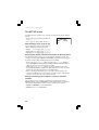
Key Notation in This Manual
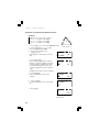
In this manual, key operations are described as follows:
To specify ex : @ " ..................... 햲
To specify In : i
To specify F : ; F ........................... 햳
To specify d/c : @ F ..................... 햲
To specify ab/c : k
To specify H : ; H ........................... 햳
To specify i
: Q .............................. 햴
햲 Functions that are printed in orange above the key require @ to be
pressed first before the key.
햳 When you specify the memory (printed in blue above the key), press
; first.
Alpha-numeric characters for input are not shown as keys but as regular
alpha-numeric characters.
햴 Functions that are printed in grey (gray) adjacent to the keys are effective
in specific modes.
Note:
• To make the cursor easier to see in diagrams throughout the manual,
it is depicted as ‘_’ under the character though it may actually appear
as a rectangular cursor on the display.
Example
Press j @ s ; R
A k S 10
• @ s and ; R means you have
to press @ followed by ` key and
; followed by 5 key.
NORMAL MODE
0.
πRŒ˚–10_
9
10
Chapter 1
Before You Get Started
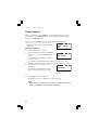
Preparing to Use the Calculator
Before using your calculator for the first time, you must reset it and adjust its
contrast.
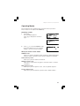
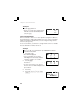
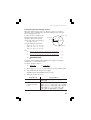
Resetting the calculator
1.
Press the RESET switch located on the
back of the calculator with the tip of a ballpoint pen or similar object. Do not use an
object with a breakable or sharp tip.
• If you do not see the message on the
right, the battery may be installed
incorrectly; refer to ‘Battery Replacement’
(See page 115.) and try installing it again.
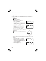
2.
Press y.
• The initial display of the NORMAL mode
appears.
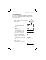
3.
Press @ o 0 and press + or
- to adjust the display contrast until it
is set correctly, then press j.
• @ o means you have to press @
followed by S key.
zALL DATA CL?z
z YES¬[DEL] z
z NO¬[ENTER]z
NORMAL MODE
0.
LCD CONTRAST
[+]
[-]
DARK® ¬LIGHT
• See ‘The OPTION menu’ (See page 118.) for more information
regarding optional functions.
11
Chapter 1: Before You Get Started
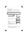
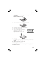
The Hard Case
Your calculator comes with a hard case to protect the keyboard and display
when the calculator is not in use.
Before using the calculator, remove the hard case and slide it onto the back
as shown to avoid losing it.
When you are not using the calculator, slide the hard case over the keyboard
and display as shown.
• Firmly slide the hard case all the way to the edge.
• The quick reference card is located inside the hard case.
• Remove the hard case while holding with fingers placed in the positions
shown below.
12
Chapter 1: Before You Get Started
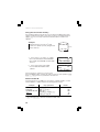
Calculator Layout and Display Symbols
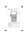
Calculator layout
1 Display screen
2 Power ON/OFF
and Clear key
3 Key operation
keys
4 Cursor keys
1 Display screen: The calculator display consists of 14 × 3 line dot matrix
display (5 × 7 dots per character) and a 2-digit exponent display per each
line.
2 Power ON/OFF and Clear key: Turns calculator ON. To turn off the
calculator, press @, then o. This key can also be used to clear the
display.
3 Key operation keys:
@: Activates the second function (printed in orange) assigned to the
next pressed key.
;: Activates the variable (printed in blue) assigned to the next
pressed key.
4 Cursor keys: Enables you to move the cursor in four directions.
13
Chapter 1: Before You Get Started
Display
Symbol
Dot matrix
display
Mantissa
Exponent
• During actual use, not all symbols are displayed at the same time.
• Only the symbols required for the usage under instruction are shown in the
display and calculation examples of this manual.
: Indicates some contents are hidden in the directions shown.
Press cursor keys to see the remaining (hidden) section.
BUSY : Appears during the execution of a calculation.
2ndF
: Appears when @ is pressed.
xy/rθ
: Indicates the mode of expression of results in the complex
calculation mode.
HYP
: Indicates that H has been pressed and the hyperbolic functions
are enabled. If @ > are pressed, the symbols ‘2ndF HYP’
appear, indicating that inverse hyperbolic functions are enabled.
ALPHA: Appears when ;, @ a, x or t is pressed.
FIX/SCI/ENG: Indicates the notation used to display a value.
DEG/RAD/GRAD: Indicates angular units.
: Appears when statistics mode is selected.
M
14
: Indicates that a value is stored in the M memory.
Chapter 1: Before You Get Started
Operating Modes
This calculator has five operating modes to perform various operations.
These modes are selected from the MODE key.
Selecting a mode
1.
Press b.
The menu display appears.
Press d to display the next menu
page.
<MODE-1>
ƒNORMAL ⁄STAT
¤PROG
‹EQN
<MODE-2>
›CPLX
2.
Press 0 to select the NORMAL mode.
• In the menu display, press the assigned
number to choose or recall a selection.
NORMAL MODE
0.
What you can do in each mode
NORMAL mode:
Allow you to perform standard scientific calculations, Differential/Integral
functions, N-base calculations, Solver function, Simulation calculation.
STAT (statistics) mode:
Allows you to perform statistical calculations.
PROG (program) mode:
Allows you to create and use programs to automate simple or complex
calculations.
EQN (equation) mode:
Allows you to perform equation solvers, such as quadratic equation.
CPLX (complex) mode:
Allows you to perform arithmetic operations with complex numbers.
15
Chapter 1: Before You Get Started
A Quick Tour
This section takes you on a quick tour covering the calculator’s simple
arithmetic operations and also principal features like the solver function.
Turning the calculator on and off
Press j at the top right of the keypad
to turn the calculator on.
1.
NORMAL MODE
0.
• To conserve the batteries, the calculator
turns itself off automatically if it is not used
for several minutes.
Press @ o to turn the calculator off.
2.
• Whenever you need to execute a function or command which is written
in orange above a key, press @ followed by the key.
Entering and solving an expression
Arithmetic expressions should be entered in the same order as they would
normally be written in. To calculate the result of an expression, press e at
the bottom right of the keypad; this has the same function as the ‘equals’ key
on some calculators.
Example
Find the answer to the expression
82 ÷ 았앙
3 – 7 × -10.5
8Az@*3NORMAL MODE
7 k S 10.5
0.
• This calculator has a minus key 8Œ©‰3-7˚–10.5_
for subtraction and a negative key S
for entering negative numbers.
• To correct an error, use the cursor keys
l r u d to move to the appropriate position on the
display and type over the original expression.
1.
2. Press e to obtain an answer.
• While the calculator is computing an
answer, BUSY is displayed at the above
left of the display.
• The cursor does not have to be at the
end of an expression for you to obtain
an answer.
16
0.
8Œ©‰3-7˚–10.5=
110.4504172
Chapter 1: Before You Get Started
Editing an expression
After obtaining an answer, you can go back to an expression and modify it
using the cursor keys just as you can before the e is pressed.
Example
Return to the last expression and change it to
82 ÷ 았3 – 7 × -10.5
Press d or r to return to the
8Œ©‰3-7˚–10.5=
last expression.
110.4504172
• The cursor is now at the beginning of
8Œ©‰3-7˚–10.5
the expression (on ‘8’ in this case).
• Pressing u or l after obtaining
an answer returns the cursor to the end
of the last expression.
• To make the cursor easier to see in diagrams throughout the manual,
it is depicted as ‘_’ under the character though it may actually appear
as a rectangular cursor on the display.
1.
Press r four times to move the
cursor to the point where you wish to
make a change.
• The cursor has moved four places to the
right and is now flashing over ‘3’.
2.
8Œ©‰3-7˚–10.5=
110.4504172
8Œ©‰3-7˚–10.5
3. Press @ O .
• This changes the character entering mode from ‘overwrite’ to ‘insert’.
• When @ is pressed the 2ndF symbol should appear at the above
of the display. If it does not, you have not pressed the key firmly
enough.
• The shape of the flashing cursor tells you which character entering
mode you are in. A triangular cursor indicates ‘insert’ mode while a
rectangular cursor indicates ‘overwrite’ mode.
Press ( and then move the cursor
to the end of expression (@ r).
• Note that the cursor has moved to the
second line since the expression now
exceeds 14 characters.
4.
5.
Press ) and e to find the
answer for the new expression.
110.4504172
8Œ©‰(3-7˚–10.5
8Œ©‰(3-7˚–10.5
)=
7.317272966
17
Chapter 1: Before You Get Started
Using variables
You can use 27 variables (A-Z and θ) in the NORMAL mode. A number
stored as a variable can be recalled either by entering the variable name or
using t.
Example 1
Store 23 to variable R.
1. Press j 2 1 then x.
• j clears the display.
• ALPHA appears automatically when you
press x. You can now enter any
alphabetic character or θ (written in blue
above keys in the keypad).
2„Ò_
2. Press R to store the result of 23 in R.
• The stored number is displayed on the
next line.
• ALPHA disappears from the display.
2„ÒR
NORMAL MODE
0.
0.
8.
You can also store a number directly
rather than storing the result of an expression.
Example 2
Find the area of a circle which has radius R.
r
S = πr 2
Enter an expression containing variable R (now equal to 8) from the last
example.
1. Press j @ s then ;.
• Whenever you need to use a character
written in blue on the keypad, press
; beforehand. ALPHA will appear at
the above of the display.
2. Press R and then A.
• ALPHA disappears after you have
entered a character.
18
NORMAL MODE
0.
π_
NORMAL MODE
0.
πRŒ_
Chapter 1: Before You Get Started
3.
Press e to obtain the result.
Follow the same procedure as above,
but press t instead of ; in
step 1.
0.
πRŒ=
201.0619298
You will get the same result.
Using simulation calculations (ALGB)
If you want to find more than one solution using the same formula or
algebraic equation, you can do this quickly and simply by use of the
simulation calculation.
Example
h
Find the volume of two cones:
1 with height 10 and radius 8 and
2 with height 8 and radius 9.
r
V=
Press j 1 k 3 @ s
; R A ; H to enter the
formula.
• Note that ‘1 3’ represents 1 over (i.e.
divided by) 3.
• Variables can be represented only by
capital letters.
1.
1 2
πr h
3
NORMAL MODE
0.
1ı3πRŒH_
Press @ G (I key) to finish
1ı3πRŒH
entering the equation.
• The calculator automatically picks out
H=z
0.
the variables alphabetically contained in
the equation in alphabetical order and
asks you to input numbers for them.
• at the bottom of the display reminds you that there is another
variable further on in the expression.
2.
Press 10 e to input the height and
go on the next variable.
• The calculator is now asking you to
input a number for the next variable.
3.
1ı3πRŒH
R=z
8.
19
Chapter 1: Before You Get Started
• Note that, as the variable R already has a number stored in memory,
the calculator recalls that number.
• indicates that there is another variable earlier in the expression.
4.
Press 8 to input the radius.
Input of all variables is now complete.
5.
Press e to obtain the solution.
•
The answer (volume of cone �) is
displayed on the third line.
Press e and 8 to input the height
for cone �.
• The display returns to a value entry
screen with ‘8’ substituted for ‘10’ in
variable H.
6.
7.
Press e to confirm the change.
1ı3πRŒH=
670.2064328
1ı3πRŒH
H=8_
1ı3πRŒH
R=z
Press 9 to enter the new radius then
press e to solve the equation.
• The volume of cone � is now displayed.
• In any step, press @ h to obtain
the solution using the values entered
into the variables at that time.
8.
8.
20
1ı3πRŒH=
678.5840132
Chapter 1: Before You Get Started
Using the solver function
You can solve any unknown variable in an equation by assigning known
values to the rest of the variables. Let us compare the differences between
the solver function and the simulation calculations using the same expression as in the last example.
Example
What is the height of cone 3 if it has a radius of 8
and the same volume as cone 2 (r = 9, h = 8) in
the last example?
h
r
V=
9.
Store the result of step 8 on the
previous page in variable V.
Press j twice and ; <
x V.
10. Input the equation (including ‘=’) in the
NORMAL mode.
Press ; V ; = then input
the rest of the expression.
You must press ; = ( m
key), not e, to enter the = sign.
11. Press I 5 to move to the
variable input display.
• Note that the values assigned to the
variables in the last example for the
simulation calculations are retained and
displayed.
12. Press d to skip the height, and
then press 8 e to enter the radius
(R).
• The cursor is now on V. The value that
was stored in step 9 is displayed.
(volume of cone 2)
13. Press u u to go back to the
variable H.
• This time the value of H from memory is
also displayed.
1 2
πr h
3
0.
AnsÒV
678.5840132
AnsÒV
678.5840132
V=1ı3πRŒH_
V=1ı3πRŒH
H=z
8.
V=1ı3πRŒH
V=z678.5840132
V=1ı3πRŒH
H=z
8.
21
Chapter 1: Before You Get Started
14. Press @ h to find the height of
H=
10.125
cone 3.
R¬
678.5840132
• Note that the calculator finds the
L¬ 678.5840132
value of the variable that the cursor is
Right and left sides of the
on when you press @ h.
expression after substituting
• Now you have the height of cone 3
the known variables
that has the same volume as cone
Height of cone 3
2.
• R→ and L→ are the values computed
by Newton's method, which is used to determine the accuracy of
the solution.
Other features
Your calculator has a range of features that can be used to perform many
calculations other than those we went through in the quick tour. Some of the
important features are described below.
Statistical calculations:
You can perform one- and two- variable weighted statistical calculations,
regression calculations, and normal probability calculations. Statistical
results include mean, sample standard deviation, population standard
deviation, sum of data, and sum of squares of data. (See Chapter 4.)
Equation solvers:
You can perform solvers of simultaneous linear equation with two/three
unknowns or quadratic/cubic equation. (See Chapter 5.)
Complex number calculations:
You can perform addition, subtraction, multiplication, and division
calculations. (See Chapter 6.)
Programming:
You can program your calculator to automate certain calculations. Each
program can be used in either the NORMAL or NBASE program modes.
(See Chapter 7.)
22
Chapter 2
General Information
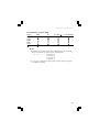
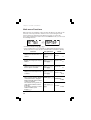
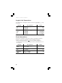
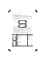
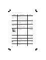
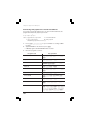
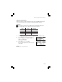
Clearing the Entry and Memories
Operation
Entry
Local
(Display) A- Z, θ*1 variables
j
Mode selection
@P0
@P1y
@P2y
×
×
×
×
×
×
×
Saved equations*2 Multi-entry
recall,
STAT*4
including saved
local variables
ANS*3 STAT VAR*5
×
×
×
×
×
×
×
×
×
× *6
×
×
@P3y
RESET switch
: Clear
*1
*2
*3
*4
*5
*6
× : Retain
Global variable memories.
Saved equations and local variables by the filing equations function
Last answer memory.
Statistical data (entered data)
n, x¯, sx, σ x, Σ x, Σ x 2, y¯ , sy, σ y, Σ y, Σ y 2, Σ xy, a, b, c, r.
Will be cleared when changing between sub-modes in the STAT mode.
Note:
• To clear one variable memory of global variable and local variable
memories, press j x and then choose memory.
Memory clear key
Press @ P to display the menu.
• To initialize the display mode, press 0.
The parameters set as follows.
• Angular unit: DEG (See page 26.)
• Display notation: NORM1 (See page 26.)
• N-base: DEC (See page 44.)
<M-CLR>
ƒDISP ⁄MEMORY
¤STAT ‹RESET
• To clear all variables (excluding local variables of saved equations,
statistical data and STAT variables), press 1 y.
• To clear statistical data and STAT variables, press 2 y.
• To RESET the calculator, press 3 y. The RESET operation will
erase all data stored in memory and restore the calculator’s default setting.
23
Chapter 2: General Information
Editing and Correcting an Equation
Cursor keys
Incorrect keystrokes can be changed by using the cursor keys
(l r u d).
Example
Enter 123456 then correct it to 123459.
1.
Press j 123456.
NORMAL MODE
0.
123456_
2. Press y 9 e.
0.
• If the cursor is located at the right end
123459=
of an equation, the y key will
123459.
function as a backspace key.
• You can return to the equation just after
getting an answer by pressing the cursor keys. After returning to the
equation, the following operations are useful;
@ l or @ r: To jump the cursor to the beginning or the
end of equation.
Overwrite mode and insert mode
• Pressing @ O switches between the two editing modes: overwrite
mode (default); and insert mode. A rectangular cursor indicates preexisting
data will be overwritten as you make entries, while a triangular cursor
indicates that an entry will be inserted at the cursor.
• In the overwrite mode, data under the cursor will be overwritten by the
number you enter. To insert a number in the insert mode, move the cursor
to the place immediately after where you wish to insert, then make the
desired entry.
• The mode set will be retained until @ O is pressed or a RESET
operation is performed.
24
Chapter 2: General Information
Delete key
• To delete a number/function, move the cursor to the number/function you
wish to delete, then press y. If the cursor is located at the right end of
an equation, the y key will function as a backspace key.
Multi-entry recall function
Previous equations can be recalled in the NORMAL, STAT or CPLX mode.
Up to 160 characters of equations can be stored in memory.
When the memory is full, stored equations are deleted in the order of the
oldest first.
• Pressing @ g will display the previous equation. Further pressing
@ g will display preceding equations.
• You can edit the equation after recalling it.
• The multi-entry memory is cleared by the following operations: mode
change, memory clear (@ P 1 y), RESET, N-base conversion.
Example
Input three expressions and then recall them.
1 3(5+2)=
2 3×5+2=
3 3×5+3×2=
1.
Press j 3 ( 5 + 2 ) e
3k 5+2e
17.
3˚5+3˚2=
21.
3k 5+3k2e
2.
Press @ g to recall the
expression 3.
3˚5+3˚2=
21.
3˚5+3˚2
3.
Press @ g to recall the
expression 2.
3˚5+3˚2=
21.
3˚5+2
4.
Press @ g to recall the
expression 1.
3˚5+3˚2=
21.
3(5+2)
25
Chapter 2: General Information
The SET UP menu
The SET UP menu enables you to change the angular unit and the display
format.
• Press @ J to display the SET UP
menu.
• Press j to exit the SET UP menu.
<SET UP>
ƒDRG
⁄FSE
¤---
Determination of the angular unit
The following three angular units (degrees,
radians, and grads) can be specified.
• DEG(°) : Press @ J 0 0
• RAD (rad): Press @ J 0 1
• GRAD (g) : Press @ J 0 2
Selecting the display notation and number of decimal places
Five display notation systems are used to display calculation results: Two
settings of Floating point (NORM1 and NORM2), Fixed decimal point (FIX),
Scientific notation (SCI) and Engineering notation (ENG).
• When @ J 1 0 (FIX) or @ J 1 2 (ENG) is
pressed, ‘TAB(0-9)?’ will be displayed and the number of decimal places
(TAB) can be set to any value between 0 and 9.
• When @ J 1 1 (SCI) is pressed, ‘SIG(0-9)?’ will be displayed and the number of significant digits (SIG) can be set to any value
between 0 and 9. Entering 0 will set a 10-digit display.
• When a floating point number does not fit in the specified range, the
calculator will display the result using the scientific notation (exponential
notation) system. See the next section for details.
Setting the floating point numbers system in scientific
notation
The calculator has two settings for displaying a floating point number:
NORM1 (default setting) and NORM2. In each display setting, a number is
automatically displayed in scientific notation outside a preset range:
• NORM1: 0.000000001 ≤ |x| ≤ 9999999999
• NORM2: 0.01 ≤ |x| ≤ 9999999999
26
Chapter 2: General Information
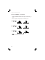
Example
100000÷3=
[Floating point (NORM1)]
→[FIXed decimal point
and TAB set to 2]
→[SCIentific notation
and SIG set to 3 ]
→[ENGineering notation
and TAB set to 2]
→[Floating point (NORM1)]
3÷1000=
[Floating point (NORM1)]
→[Floating point (NORM2)]
→[Floating point (NORM1)]
Key operations
Result
j@J13
100000 z 3 e
@J102
33333.33333
33333.33
04
@J113
3.33˚10
@J122
33.33˚10
@J13
03
33333.33333
j 3 z 1000 e
@J14
@J13
0.003
-03
3.˚10
0.003
Using Memories
The calculator uses global variable memories (A–Z and θ), local variable
memories (maximum of nine variables per equation), and a last answer
memory used when solving equations.
Using alphabetic characters
You can enter an alphabetic character (written
in blue) when ALPHA is displayed at the top of
the display. To enter this mode, press ;.
To enter more than one alphabetic character,
press @ a to apply the alphabet-lock
mode. Press ; to escape from this mode.
NORMAL MODE
0.
Using global variables
You can assign values (numbers) to global variables by pressing x then
A–Z and θ.
Example 1
Store 6 in global variable A.
1.
Press j 6 x A.
• There is no need to press ; because
ALPHA is selected automatically when
you press x.
0.
6ÒA
6.
27
Chapter 2: General Information
Example 2
Recall global variable A.
1. Press t A.
• There is no need to press ; because
ALPHA is selected automatically when
you press t.
6.
A=
6.
Using local variables
Nine local variables can be used in each equation or program, in addition to
the global variables. Unlike global variables, the values of the local variables
will be stored with the equation when you save it using the filing equations
function. (See page 58.)
To use local variables, you first have to assign the name of the local variable
using two characters: the first character must be a letter from A to Z or θ and
the second must be a number from 0 to 9.
Example
Store 1.25 x 10-5 as local variable A1 (in the NORMAL mode) and
recall the stored number.
1. Press @ v.
• The VAR menu appears.
• If no local variables are stored yet,
ALPHA appears automatically and the
calculator is ready to enter a name.
2. Press A1 e.
• ¬ shows that you have finished assigning
the name A1.
• To assign more names, press d to
move the cursor to VAR 1 and repeat the
process above.
ƒz
⁄
¤
‹
›
fi
fl
‡
°
¬ƒA¡ ‹
⁄
›
¤
fi
fl
‡
°
3. Press j.
• This returns you to the previous screen.
4.
28
Press 1.25 ` S 5 x @
v 0.
0.
1.25E–5ÒA1
0.0000125
Chapter 2: General Information
• You do not need to enter an alphabetic character. Just specify the
named local variable using a number from 0 to 8, or move the arrow
to the appropriate variable the press e.
5. Press @ v 0 e.
• The value of VAR 0 will be recalled.
• Alternatively you can recall a variable by
moving the arrow to it then press e
twice.
0.0000125
A1=
0.0000125
Note:
• You can change the name of a local variable by overwriting it in the VAR
menu. The cursor appears when r is pressed in the VAR menu.
• Local variables not stored using the filing equations function will be
deleted by mode selection or memory clear operation (@ P
1 y).
• Local and global variables will be cleared by creating a new program,
and editing and running a program.
Using variables in an equation or a program
Both global and local variables can be used directly in an equation or a
program. Local variables are useful when you need to use variables such as
X1 and X2 at the same time in another equation. The local variable names
and their values can be saved in each equation. (See page 58.)
Example
Using A (6) and A1 (0.0000125) from the last two examples, solve the
expression.
1
— – 1000A
A1
1. Press j 1 k.
• Start entering the expression.
NORMAL MODE
0.
1ı_
2.
Press @ v.
3. Press 0 - 1000 ; A e.
• The display returns automatically to the
previous screen after you have chosen
the local variable, and you can continue
to enter the expression.
• You do not need k if you use a
variable. However, the variable must be
a multiplier.
¬ƒA¡ ‹
⁄
›
¤
fi
fl
‡
°
0.
1ıA¡-1000A=
74000.
29
Chapter 2: General Information
Using the last answer memory
The calculator always keeps the most recent answer in ANS memory and
replaces it with the new answer every time you press an ending instruction
(e, x etc.). You may recall the last answer and use it in the next
equation.
Example
Evaluate the base area (S = 32π) and
volume of a cylinder (V = 5S) using the last
answer memory.
h=5
r=3
1. Press j 3 A @ s e.
• The area of the base is now calculated.
• The number 28.27433388 is held in ANS
memory.
0.
3ι=
28.27433388
2. Press j 5 ; < e.
• You now have the volume of the
cylinder.
0.
5Ans=
141.3716694
The last answer is cleared (i.e. set to 0) if you
press the RESET switch, change the mode or memory clear operation (@
P 1 y), but not if you turn the calculator off.
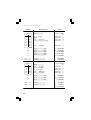
Global variable M
Using the M memory, in addition to the features of global variables, a value
can be added to or subtracted from an existing memory value.
Example
$150×3:Ma
+)$250:Mb=Ma+250
–)Mb×5%
M
Key operations
jxM
150 k 3 m
250 m
t Mk 5@ %
@MtM
• m and @ M cannot be used in the STAT mode.
30
Result
0.
450.
250.
35.
665.
Chapter 2: General Information
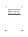
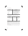
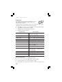
Using memory in each mode
Mode
ANS
M
A-L, N-Z,
Local variables
NORMAL
STAT
PROG
EQN
CPLX
: Available
: Unavailable
Notes:
• Calculation results from the functions indicated below are automatically stored in memories replacing any existing values.
• →r θ, →xy.................. R memory (r)
θ memory (θ)
X memory (x)
Y memory (y)
• Use of t or ; will recall the value stored in memory using up
to 14 digits in accuracy.
31
Chapter 2: General Information
Resetting the calculator
If you wish to clear all memories, variables, files and data, or if none of the
keys (including j) will function, press the RESET switch located on the
back of the calculator.
In rare cases, all the keys may cease to function if the calculator is subjected
to strong electrical noise or heavy shock during use. Follow the instructions
below to reset the calculator.
Caution:
• The RESET operation will erase all data stored in memory and
restore the calculator's default setting.
1.
Press the RESET switch located on the
back of the calculator with the tip of a ballpoint pen or similar object. Do not use an
object with a breakable or sharp tip.
• A display appears asking you to confirm
that you really want to reset the calculator.
Press y.
2.
• All memories, variables, files and data are
cleared.
• The display goes back to the initial display in
the NORMAL mode.
• The calculator will revert to the very first
settings that were made when you started
to use the calculator for the first time.
zALL DATA CL?z
z YES¬[DEL] z
z NO¬[ENTER]z
z ALL DATA z
z CLEARED! z
z
z
NORMAL MODE
0.
Or, to cancel the operation, press e.
Note:
• When corruption of data occurs, the reset procedure may automatically be initiated upon pressing the RESET switch.
• Pressing @ P and 3 y can also clear all memories,
variables, files and data as described above.
32
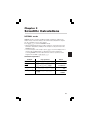
Chapter 3
Scientific Calculations
NORMAL mode
NORMAL mode is used for standard scientific calculations, and has the
widest variety of functions. Many of the functions described in this chapter
are also available for use in other modes.
Press b 0 to select the NORMAL mode.
• Differential/Integral functions, N-base functions, Solver functions and
Simulation Calculation (ALGB) in this chapter are all performed in the
NORMAL mode.
• In each example of this chapter, press j to clear the display first. If
the FIX, SCI or ENG indicator is displayed, clear the indicator by
selecting ‘NORM1’ from the SET UP menu. Unless specified, set the
angular unit as ‘DEG’. (@ P 0)
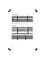
Arithmetic operations
Example
Key operations
45+285÷3=
j 45 + 285 z 3 e
18+6
=
15–8
( 18 + 6 ) z
( 15 - 8 ) e
42×(–5)+120=
42 k S 5 + 120 e
3
–3
(5×10 )÷(4×10 )=
5` 3z 4` S
3e
Result
140.
3.428571429
–90.
1250000.
33
Chapter 3: Scientific Calculations
Constant calculations
Example
Key operations
Result
34+57=
34 + 57 e
91.
45+57=
45
e
102.
68×25=
68 k 25 e
1700.
68×40=
40 e
2720.
• In constant calculations, the addend becomes a constant. Subtraction
and division behave the same way. For multiplication, the multiplicand
becomes a constant.
• In constant calculations, constants will be displayed as ∆.
Functions
Example
Key operations
Result
sin60 [°]=
j v 60 e
0.866025403
π
cos — [rad]=
4
@J01$
@ s k 4e
0.707106781
–1
tan 1 [g]=
@J02@y1
e
@P0
50.
• The range of the results of inverse trigonometric functions
DEG
RAD
GRAD
34
θ = sin–1 x, θ= tan–1 x
θ = cos–1 x
–90 ≤ θ ≤ 90
0 ≤ θ ≤ 180
π
π
—
–—
2 ≤θ≤ 2
–100 ≤ θ ≤ 100
0 ≤θ≤π
0 ≤ θ ≤ 200
Chapter 3: Scientific Calculations
Example
Key operations
Result
(cosh 1.5 +
sinh 1.5)2 =
j ( H $ 1.5 +
H v 1.5 ) A e
20.08553692
5
tanh–1— =
7
@>t(5
z 7) e
0.895879734
ln 20 =
i 20 e
2.995732274
log 50 =
l 50 e
1.698970004
e3 =
@ " 3e
20.08553692
101.7 =
@ Y 1.7 e
50.11872336
1
1
—+—=
6
7
6 @ Z + 7@
Ze
0.309523809
8 –3 ×5 =
–2
4
2
8m S 2- 3m
4k 5A e
4=
(123)—
12 m 3 m 4
@Ze
83 =
81 e
1
49 –
3
4
81 =
27 =
4! =
-2024.984375
6.447419591
512.
@ * 49 - 4 @ D
81 e
4.
@ q 27 e
3.
4@ B e
24.
P3 =
10 @ e 3 e
720.
5
C2 =
5@ c 2e
10.
500×25%=
500 k 25 @ %
125.
120÷400=?%
120 z 400 @ %
30.
500+(500×25%)=
500 + 25 @ %
625.
400–(400×30%)=
400 - 30 @ %
280.
10
35
Chapter 3: Scientific Calculations
Math menu Functions
Other functions are available on this calculator besides the first and second
functions on the key pad. These functions are accessed using the math
function menu. The math menu has different contents for each mode.
Press I to display the math menu. In the NORMAL mode, you can recall
the following functions.
<MATH MENU-1>
ƒabs ⁄ipart
¤int ‹fpart
→ <MATH MENU-2>
d
›ÒRAND fiSOLVE
flΩsec ‡Ωmin
• Switch the display using d u.
• These math menus are not available for Differential/Integral functions,
N-base functions, Solver functions and Simulation Calculation (ALGB).
Function
Key operations
Result
0: abs
Displays the absolute value of a
number.
I0S
7e
abs–7=
1: ipart
Displays the integer part only of a
number.
I1S
7.94 e
ipart–7.94=
–7.
2: int
Displays the largest integer less
than or equal to a number.
I2S
7.94 e
int–7.94=
3: fpart
Displays the fractional part only of
a number.
I3S
7.94 e
fpart–7.94=
–0.94
4: ⇒RAND
Before using the Random Numbers 0.001 I 4
of Random functions, designate
0.001 from 0.999 random number
sequences available.
The calculator can regenerate the
same random numbers from the
@w0
beginning.
e
If you wish to go back to normal
random numbers, press
0 I 4.
36
7.
–8.
0.001ÒRAND
0.001
random=
0.232
Chapter 3: Scientific Calculations
Function
5: SOLVE
Enter the Solver function mode.
(See page 52.)
Key operations
I 5
Result
6: Ωsec
Sexagesimal numbers are
converted to seconds notation.
(See page 46.)
24 [ I
6
24∂Ωsec
7: Ωmin
Sexagesimal numbers are
converted to minutes notation.
(See page 46.)
0[0[
1500 I 7
0∂0∂1500Ωmin
25.
86400.
37
Chapter 3: Scientific Calculations
Differential/Integral Functions
Differential and integral calculations can only be performed in the NORMAL
mode. It is possible to reuse the same equation over and over again and to
recalculate by only changing the values without having to re-enter the
equation.
•
•
•
•
Performing a calculation will clear the value in the X memory.
You can use both global and local variables in the equation.
The answer calculated will be stored in the last answer memory.
The answer calculated may include a margin of error, or an error may
occur. In such a case, recalculate after changing the minute interval (dx)
or subinterval (n).
• Since differential and integral calculations are performed based on the
following equations, in certain rare cases correct results may not be
obtained, such as when performing special calculations that contain
discontinuous points.
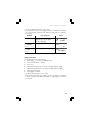
Integral calculation (Simpson’s rule):
1
S=—h{f (a)+4{f (a+h)+f (a+3h)+······+f (a+(N–1)h)}
3
+2{f (a+2h)+f (a+4h)+······+f (a+(N–2)h)}+f(b)}
b–a
h= ——
N
N=2n
a ≤x≤ b
Differential calculation:
dx
dx
f(x+ ––)–f(x–
––)
2
2
f’(x)=————————
dx
Differential function
The differential function is used as follows.
1.
Press b 0 to enter the NORMAL mode.
2.
Input a formula with an x variable.
3.
Press @ 3.
4.
Input the x value and press e.
5.
Input the minute interval (dx).
6.
Press e to calculate.
38
Chapter 3: Scientific Calculations
• To exit the differential function, press j.
• After getting the answer, press e to return to the display for inputting
the x value and the minute interval, and press @ h to recalculate
at any point.
Example
Key operations
d/dx (x4–0.5x3+6x2)
j ; X* m 4 - 0.5
;X1+6;
XA@3
x=2
dx = 0.00002
d/dx = ?
2ee
x=3
dx = 0.001
d/dx = ?
e 3 e 0.001 e
Result
≈^4-0.5≈„+6≈Œ
0.
≈=z
dx:
0.00001
≈^4-0.5≈„+6≈Œ
d/dx=
50.
≈^4-0.5≈„+6≈Œ
d/dx=
130.5000029
* X memory is specified by pressing ; then the 3 key.
Integral function
The Integral function is used as follows.
1.
Press b 0 to enter the NORMAL mode.
2.
Input a formula with an x variable.
3.
Press {.
4.
Input the starting value (a) of a range of integral and press e.
5.
Input the finishing value (b) of a range of integral and press e.
6.
Input the subinterval (n).
7.
Press e to calculate.
• To exit the integral function, press j.
• After getting the answer, press e to return to the display for inputting
a range of integral and subinterval, and press @ h to recalculate
at any point.
39
Chapter 3: Scientific Calculations
Example
8
Key operations
Result
∫ 2 (x2–5)dx
j;XA-5
{
a=z
b=
n=
n = 100
∫ dx = ?
2e8ee
≈Œ-5
∫dx=
n = 10
∫ dx = ?
e e e 10 e
0.
0.
100.
138.
≈Œ-5
∫dx=
138.
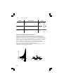
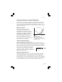
When performing integral calculations
Integral calculations require a long calculation time, depending on the
integrands and subintervals input. During calculation, ‘calculating!’ will be
displayed. To cancel calculation, press j. Note that there will be greater
integral errors when there are large fluctuations in the integral values during
minute shifting of the integral range and for periodic functions, etc., where
positive and negative integral values exist depending on the interval.
For the former case, make the integral interval as small as possible. For the
latter case, separate the positive and negative values.
Following these tips will provide calculations results with greater accuracy
and will also shorten the calculation time.
y
x0
y
x2
b
a
40
x0 x 1
x2
x3
bx
a
x
x1
x3
Chapter 3: Scientific Calculations
Random Function
The Random function has four settings for the NORMAL, STAT or PROG
mode. (This function is not available while using the N-base function, solver
function and simulation calculations.)
Random numbers
A pseudo-random number, with three significant digits from 0 up to 0.999,
can be generated by pressing @ w 0 e. To generate further
random numbers in succession, press e. Press j to exit.
• The calculator can regenerate the same random number. (See page 36.)
Random dice
To simulate a die-rolling, a random integer between 1 and 6 can be generated by pressing @ w 1 e. To generate further random
numbers in succession, press e. Press j to exit.
Random coin
To simulate a coin flip, 0 (head) or 1 (tail) can be randomly generated by
pressing @ w 2 e. To generate further random numbers in
succession, press e. Press j to exit.
Random integer
An integer between 0 and 99 can be generated randomly by pressing @
w 3 e. To generate further random numbers in succession, press
e. Press j to exit.
Example
Pick a random
number between
0 and 9.99.
Key operations
j@w0
k 10 e
Result
0.
random˚10=
6.31
• The result may not be the same each time this operation is performed.
41
Chapter 3: Scientific Calculations
Angular Unit Conversions
The angular unit is changed in sequence each time @ ] ( . key)
is pressed.
Example
Key operations
Result
90°→ [rad]
→ [g]
→ [°]
j 90 @ ]
@]
@]
1.570796327
100.
90.
sin–10.8 = [°]
→ [rad]
→ [g]
→ [°]
@ w 0.8 e
@]
@]
@]
53.13010235
0.927295218
59.03344706
53.13010235
Chain Calculations
The previous calculation result can be used in a subsequent calculation.
However, it cannot be recalled after entering multiple instructions.
• When using postfix functions (
, sin, etc.), a chain calculation is
possible even if the previous calculation result is cleared by the use of
the j key.
Example
Key operations
6+4=ANS
ANS+5
j6+4e
+5e
8×2=ANS
ANS2
8k2e
Ae
44+37=ANS
ANS=
44 + 37 e
@*e
42
Result
10.
15.
16.
256.
81.
9.
Chapter 3: Scientific Calculations
Fraction Calculations
Arithmetic operations and memory calculations can be performed using
fractions, and conversions between decimal numbers and fractions.
• If the number of digits to be displayed is greater than 10, the number is
converted to and displayed as a decimal number.
Example
1
4
b
3— + — = [a—]
c
2
3
→[a.xxx]
→[d/c]
2
—
10 3 =
5
(—75 ) =
1
—
3
(—18 )
Key operations
Result
j3k1k2+
4k3e
k
@F
4ı5ı6 *
4.833333333
29ı6
@Y2k3e
4.641588834
7k5m5e
16807ı3125
1k8m1k3e
1ı2
@ * 64 k 225 e
8ı15
23
—=
34
(2m3)k
(3m4)e
8ı81
1.2
—– =
2.3
1.2 k 2.3 e
1°2’3”
——– =
2
1[2[3k2e
0∂31∂1.5∂
1×103
——– =
2×103
1`3k2`3e
1ı2
=
64
—— =
225
A=7
4
—=
A
2
1.25 + — = [a.xxx]
5
b
→[a—]
c
5
* 4ı5ı6 = 4—
6
j7xA
4k;Ae
1.25 + 2 k 5 e
k
12ı23
7.
4ı7
1.65
1ı13ı20
43
Chapter 3: Scientific Calculations
Binary, Pental, Octal, Decimal, and Hexadecimal
Operations (N-base)
This calculator can perform conversions between numbers expressed in
binary, pental, octal, decimal and hexadecimal systems. It can also perform
the four basic arithmetic operations, calculations with parentheses and
memory calculations using binary, pental, octal, decimal, and hexadecimal
numbers. Furthermore, the calculator can carry out the logical operations
AND, OR, NOT, NEG, XOR and XNOR on binary, pental, octal and hexadecimal numbers.
Conversion to each system is performed by the following keys:
@ z: Converts to the binary system. ‘?’ appears.
@ r: Converts to the pental system. ‘q’ appears.
@ g: Converts to the octal system. ‘f’ appears.
@ h: Converts to the hexadecimal system. ‘6’ appears.
@ /: Converts to the decimal system. ‘?’, ‘q’, ‘f’ and ‘6’ disappear
from the display.
Conversion is performed on the displayed value when these keys are
pressed.
Note: Hexadecimal numbers A – F are entered into the calculator by
pressing ,, m, A, 1, l, and i key respectively.
In the binary, pental, octal, and hexadecimal systems, fractional parts cannot
be entered. When a decimal number having a fractional part is converted
into a binary, pental, octal, or hexadecimal number, the fractional part will be
truncated. Likewise, when the result of a binary, pental, octal, or hexadecimal
calculation includes a fractional part, the fractional part will be truncated. In
the binary, pental, octal, and hexadecimal systems, negative numbers are
displayed as a complement.
44
Chapter 3: Scientific Calculations
Example
Key operations
Result
DEC(25)→BIN
j @ / 25 @ z
HEX(1AC)
→BIN
→PEN
→OCT
→DEC
@ a 1AC
@z
@r
@g
@/
BIN(1010–100)
×11 =
@ z ( 1010 - 100
) k 11 e
BIN(111)→NEG
d 111 e
HEX(1FF)+
OCT(512)=
HEX(?)
@ a 1FF @ g +
512 e
@a
2FEC–
2C9E=(A)
+)2000–
1901=(B)
(C)
j x M @ a 2FEC
- 2C9Em
2000 1901 m
tM
1011 AND
101 = (BIN)
j @ z 1011 4
101 e
1.b
5A OR C3 = (HEX)
@ a 5A p C3 e
DB.H
NOT 10110 =
(BIN)
@ z n 10110 e
1111101001.b
24 XOR 4 = (OCT)
@ g 24 x 4 e
B3 XNOR
2D = (HEX)
→DEC
@ a B3 C
2D e
@/
11001.b
110101100.b
3203.P
654.0
428.
10010.b
1111111001.b
1511.0
349.H
34E.H
6FF.H
A4D.H
20.0
FFFFFFFF61.H
–159.
45
Chapter 3: Scientific Calculations
Time, Decimal and Sexagesimal Calculations
Conversion between decimal and sexagesimal numbers can be performed,
and, while using sexagesimal numbers, also conversion to seconds and
minutes notation. The four basic arithmetic operations and memory calculations can be performed using the sexagesimal system. Notation for
sexagesimal is as follows:
12∂34∂56.78∂
degree
Example
minute
second
Key operations
12°39’18.05”
→[10]
j 12 [ 39 [ 18.05
@:
123.678→[60]
123.678 @ :
3h30m45s +
6h45m36s = [60]
3 [ 30 [ 45 + 6 [
45 [ 36 e
1234°56’12” +
0°0’34.567” = [60]
1234 [ 56 [ 12 +
0 [ 0 [ 34.567 e
3h45m –
1.69h = [60]
3 [ 45 - 1.69 e
@:
sin62°12’24” = [10]
v 62 [ 12 [ 24 e
24°→[ ” ]
24 [ I 6
1500”→[ ’ ]
0 [ 0 [ 1500 I 7
46
Result
12.65501389
123∂40∂40.8∂
10∂16∂21.∂
1234∂56∂47.∂
2∂3∂36.∂
0.884635235
86400.
25.
Chapter 3: Scientific Calculations
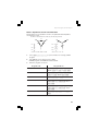
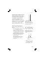
Coordinate Conversions
Conversions can be performed between rectangular and polar coordinates.
Y
P (x, y)
Y
r
P (r, θ)
y
0
x
X
Rectangular coordinate
0
θ
X
Polar coordinate
• Before performing a calculation, select the angular unit.
• The calculation result is automatically stored in memories.
• Value of r: R memory
• Value of θ: θ memory
• Value of x: X memory
• Value of y: Y memory
• r and x values are stored in the last answer memory.
Example
Key operations
Result
x=6
r=
→
θ = [°]
y=4
j6,4
@u
r= 7.211102551
= 33.69006753
r = 14
14 , 36
@E
x= 11.32623792
y= 8.228993532
θ = 36[°]
→
x=
y=
47
Chapter 3: Scientific Calculations
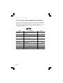
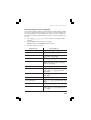
Calculations Using Physical Constants
Recall a constant by pressing @ c followed by the number of the
physical constant designated by a 2-digit number.
The recalled constant appears in the display mode selected with the
designated number of decimal places.
Physical constants can be recalled in the NORMAL mode (when not set to
binary, pental, octal, or hexadecimal), STAT mode, PROG mode and EQN
mode.
Note: Physical constants are based either on the 2002 CODATA recommended values, or the 1995 Edition of the ‘Guide for the Use of the
International System of Units (SI)’ released by NIST (National Institute
of Standards and Technology), or on ISO specifications.
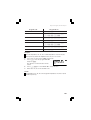
No.
01
02
03
04
05
06
07
08
09
10
11
12
13
14
15
16
17
18
19
20
21
22
23
48
Constant
Speed of light in vacuum
Newtonian constant of gravitation
Standard acceleration of gravity
Electron mass
Proton mass
Neutron mass
Muon mass
Atomic mass unit-kilogram relationship
Elementary charge
Planck constant
Boltzmann constant
Magnetic constant
Electric constant
Classical electron radius
Fine-structure constant
Bohr radius
Rydberg constant
Magnetic flux quantum
Bohr magneton
Electron magnetic moment
Nuclear magneton
Proton magnetic moment
Neutron magnetic moment
Symbol
c, c 0
G
gn
me
mp
mn
mµ
lu
e
h
k
µ0
ε0
re
α
a0
R∞
Φ0
µB
µe
µN
µp
µn
Unit
m s–1
m3 kg–1 s–2
m s–2
kg
kg
kg
kg
kg
C
Js
J K–1
N A–2
F m–1
m
m
m–1
Wb
J T–1
J T–1
J T–1
J T–1
J T–1
Chapter 3: Scientific Calculations
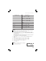
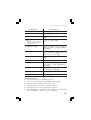
No.
24
25
26
27
28
29
30
31
32
33
34
35
36
37
38
39
40
41
42
43
44
45
46
47
48
49
50
51
52
Constant
Symbol
Muon magnetic moment
Compton wavelength
Proton Compton wavelength
Stefan-Boltzmann constant
Avogadro constant
Molar volume of ideal gas (273.15 K,
101.325 kPa)
Molar gas constant
Faraday constant
Von Klitzing constant
Electron charge to mass quotient
Quantum of circulation
Proton gyromagnetic ratio
Josephson constant
Electron volt
Celsius Temperature
Astronomical unit
Parsec
Molar mass of carbon-12
Planck constant over 2 pi
Hartree energy
Conductance quantum
Inverse fine-structure constant
Proton-electron mass ratio
Molar mass constant
Neutron Compton wavelength
First radiation constant
Second radiation constant
Characteristic impedance of vacuum
Standard atmosphere
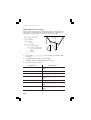
Example
V0 = 15.3 m/s
t = 10 s
1 2
V0 t +
gt = ? m
2
µµ
Unit
–1
λc
λc, p
σ
NΑ, L
JT
m
m
W m–2 K–4
mol–1
Vm
m3 mol–1
R
F
RK
-e/me
h/2me
γp
KJ
eV
t
AU
pc
M(12C)
-h
J mol–1 K–1
C mol–1
Ohm
C kg–1
m2 s–1
s –1 T–1
Hz V–1
J
K
m
m
kg mol–1
Eh
Js
J
G0
s
mp/me
Mu
kg mol–1
λc, n
c1
c2
m
W m2
mK
α –1
Z0
Key operations
j 15.3 k 10 + 2 @
Z k @ c 03 k 10
Ae
Ω
Pa
Result
643.3325
49
Chapter 3: Scientific Calculations
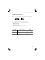
Calculations Using Engineering Prefixes
Calculation can be executed in the NORMAL mode (excluding N-base),
STAT mode and PROG mode using the following 12 types of prefixes.
Prefix
E
P
T
G
M
k
m
µ
n
p
f
a
(Exa)
(Peta)
(Tera)
(Giga)
(Mega)
(kilo)
(milli)
(micro)
(nano)
(pico)
(femto)
(atto)
Example
100m × 10k =
50
Operation
@j0
@j1
@j2
@j3
@j4
@j5
@j6
@j7
@j8
@j9
@jA
@jB
Key operations
100 @ j 6 k
10 @ j 5 e
Unit
1018
1015
1012
109
106
103
10–3
10–6
10–9
10–12
10–15
10–18
Result
1000.
Chapter 3: Scientific Calculations
Modify Function
Calculation results are internally obtained in scientific notation with up to 14
digits for the mantissa. However, since calculation results are displayed in
the form designated by the display notation and the number of decimal
places indicated, the internal calculation result may differ from that shown in
the display. By using the modify function, the internal value is converted to
match that of the display, so that the displayed value can be used without
change in subsequent operations.
Example
5÷9=ANS
ANS×9=
[FIX,TAB=1]
Key operations
j@J101
5z9e
k 9 e*1
5z9e@n
k 9 e*2
@P0
Result
0.6
5.0
0.6
5.4
*1 5.5555555555555×10–1×9
*2 0.6×9
51
Chapter 3: Scientific Calculations
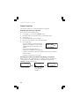
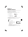
Solver Function
This function enables you to find any variable in an equation.
Entering and solving an equation
The solver function is used as follows.
1.
Press b 0 to enter the NORMAL mode.
2.
Enter both sides of an equation, using ‘=’ and variable names.
3.
Press I 5.
4.
Enter the value of the known variables.
5.
Move the cursor (display) to the unknown variables.
Press @ h.
6.
• The solver function can find any variable
anywhere in an equation. It can even find
variables that appear several times in an
equation.
• You can use both global and local
variables in your equation. (See page 58.)
NORMAL MODE
0.
TŒ=(4π©GM)R_
Equation entering display
• Using the solver function will cause variables memory to be overwritten
with new values.
• To exit the solver function, press j.
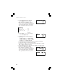
Changing the value of variables and editing an equation
When you are in the solution display, press e to return to the display for
entering values of variables, then return to the equation display in the
NORMAL mode by pressing j.
R= 1.127251652
R¬
9.
L¬
9.
Solution display
52
TŒ=(4π©GM)R
→
e G=z
1.5
Use d u to
move between
variables.
NORMAL MODE
0.
→
j TŒ=(4π©GM)R_
Chapter 3: Scientific Calculations
Solving an equation
Example
Try finding the variables in the equation below.
A×B = C × D
1.
Press b 0 to select the NORMAL mode.
Press ; A k ; B ;
= ; C k ; D.
• You must enter the whole equation.
2.
NORMAL MODE
0.
A˚B=C˚D_
3. Press I 5.
• The calculator automatically calls the
A˚B=C˚D
display for entering variables and
displays the variables in alphabetical
A=z
0.
order.
• indicates that there are more
variables.
• If a variable already has a value, the calculator displays that value
automatically.
4. Press 10 e.
• Enters a value for known variable A.
• The cursor moves onto the next
variable.
5. Press 5 e.
• Enters a value for known variable B.
A˚B=C˚D
B=z
A˚B=C˚D
C=z
6. Press 2.5 e.
• Enters a value for known variable C.
• The cursor moves onto the next
variable. indicates that this is the last
variable.
7. Press @ h.
• After showing the ‘calculating!’ display,
the calculator finds the value for the
unknown variable that was indicated
by the cursor.
0.
0.
A˚B=C˚D
D=z
0.
D=
R¬
L¬
20.
50.
50.
Values of the left-hand side
of the equation
Values of the right-hand side
of the equation
53
Chapter 3: Scientific Calculations
• The value shown on the display for the unknown variable does not
have to be set to 0 to solve the equation.
• The answer is displayed on the top line and the values of the lefthand and right-hand sides of the equation appear below.
8. Press e.
• Returns you to the display for entering
variables.
9. Press d 8 e.
• Substitutes the value 8 for B.
• The cursor moves onto the next variable
C.
10. Press @ h.
• You can find any unknowns in the same
equation.
A˚B=C˚D
A=z
10.
A˚B=C˚D
C=z
2.5
C=
R¬
L¬
4.
80.
80.
Important notes
There are several important points to remember when you use the solver
function.
• To cancel calculation, press j when ‘calculating!’ is displayed.
• Before entering the equation, the appropriate angular unit must be
selected.
• The calculator uses Newton’s method to solve equations. Due to this,
there may be some equations that it fails to solve even though they are
in fact solvable. (See page 123.)
• The calculator stops calculating when the values it has obtained for the
left and right sides of the equation become very close. Thus in certain
cases the solution it gives may not be the real answer. (See page 122.)
• In certain cases, the calculator may abort a calculation and display the
message shown on the right. (See page
- ERROR 02 121.)
CALCULATION
54
Chapter 3: Scientific Calculations
Simulation Calculation (ALGB)
This function enables you to find different solutions quickly using different
sets of values in the same expression.
Entering an expression for simulation calculation
The simulation calculation is used as follows.
1.
Press b 0 to enter the NORMAL mode.
2.
Enter an expression with at least one variable.
3.
Press @ G.
4.
Enter the values of the variables. The calculation result will be displayed
after entering the value for all used variables.
• You can use both global and local variables in your equation, but only
local variables will be stored if you save the equation. (See page 58.)
• You need enter only the side of the equation that contains the variables.
• Performing simulation calculation will cause the variables memories to
be overwritten with new values.
• The answer calculated will be stored in last answer memory.
• To exit simulation calculation, press j.
Changing a value of variables and editing an expression
When you are in the solution display, press e to return to the display for
entering values of variables, then return to the equation display in the
NORMAL mode by pressing j.
πRŒH=
785.3981634
Solution display
πRŒH
→
e H=z
NORMAL MODE
5.
→
j πRŒH_
0.
Use d u to
move between
variables.
55
Chapter 3: Scientific Calculations
Simulate an equation for different values
Example
Find the area S = bc sin A ÷ 2 when:
A
1 b = 3, c = 5 and A = 90° (DEG)
2 b = 3, c = 5 and A = 45° (DEG)
3 b = 4, c = 5 and A = 45° (DEG)
1.
S
Press b 0 to select the NORMAL mode.
2. Press @ J 0 0 j.
• Sets the angular unit to DEG.
Press ; B ; C v
; A z 2.
• The equation is entered in the normal
way.
3.
4. Press @ G.
• The calculator automatically calls the
display for entering variables and picks
out the variables in alphabetical order.
• If a variable already has a value, the
calculator displays that value automatically.
• indicates that there are more variables.
5. Press 90 e.
• The calculator picks out the next
variable.
6.
•
Press 3 e 5.
indicates that this is the last variable.
c
b
S = bc sin A ÷ 2
NORMAL MODE
0.
BCsinA©2_
BCsinA©2
A=z
0.
BCsinA©2
B=z
0.
BCsinA©2
C=5_
7. Press e.
BCsinA©2=
7.5
Area of triangle 1 is 7.5
square units.
56
Chapter 3: Scientific Calculations
8. Press e and then 45 e.
• After getting the answer, press e to
return to the display for entering
variables.
9. Press @ h.
• Sides b and c are both the same length
in triangle 2 as in triangle 1, so you do
not have to re-enter these values.
2BCsinA©2
B=z
3.
BCsinA©2=
5.303300859
Area of triangle 2 is
displayed.
10. Press e and then d 4 e
@ h.
BCsinA©2=
7.071067812
Area of triangle 3 is
displayed.
57
Chapter 3: Scientific Calculations
Filing Equations
When the calculator is in the NORMAL mode (excluding N-base), you can
save equations in the EQUATION FILE. Saved equations can be loaded or
deleted in the NORMAL mode.
Press f in the NORMAL mode to call the EQUATION FILE menu.
• Press 0, 1 or 2 to select if an
equation is to be loaded, saved or deleted,
respectively.
<EQTN FILE>
ƒLOAD ⁄SAVE
¤DEL
Saving an equation
You can save an equation as follows.
1.
After entering an equation in the NORMAL
mode, press 1 in the EQUATION FILE
menu.
SAVE:TITLE?
• The file name display appears asking you
to enter a title.
• The calculator automatically locks ALPHA on to enable you to enter
alphabetic characters easily. To cancel the ALPHA setting, press ;.
2.
Enter the title of the file (up to seven
characters).
• If you change your mind and no longer
want to save the equation, press j.
SAVE:RING_
“RING” is entered as the
file name.
Press e to save the equation.
3.
• The display returns to the display before pressing f.
Note:
• When saving an equation, local variables (including their values)
used in the equation are saved at the same time.
58
Chapter 3: Scientific Calculations
Loading and deleting an equation
The procedures to retrieve (load) and delete an equation from memory are
the same, except that you have to confirm that you wish to delete the
equation.
Retrieve or delete an equation as follows.
1.
Press f and then 0 or 2 to
retrieve (load) or delete.
2.
Use d u to select the name of the
file you wish to retrieve (or delete),and
press e.
DEL ¬º⁄RING
º¤AREA-3
º‹CIRCUIT
DEL has been selected.
• The display asks for confirmation if you
are deleting an equation. Press y to
proceed with deletion or e to cancel
the operation.
TITLE:RING
DELETE¬[DEL]
QUIT¬[ENTER]
Note:
• If the equation being retrieved contains local variables, the local
variable names and their values will be retrieved along with the
equation.
• Any other equation on the display and local variables before the
equation was retrieved are cleared.
59
60
Chapter 4:
Statistical Calculations
The STAT mode is used to perform statistical calculations.
Press b 1 to select the statistics mode. The seven statistical
calculations listed below can be performed. After selecting the statistics
mode, select the desired sub-mode by pressing the number key that
corresponds to your choice.
To change statistical sub-mode, reselect statistics mode (press b 1),
then select the required sub-mode.
0 (SD)
: Single-variable statistics
1 (LINE)
: Linear regression calculation
2 (QUAD)
: Quadratic regression calculation
3 (EXP)
: Exponential regression calculation
4 (LOG)
: Logarithmic regression calculation
5 (POWER) : Power regression calculation
6 (INV)
: Inverse regression calculation
61
Chapter 4: Statistical Calculations
The following statistics can be obtained for each statistical calculation (refer
to the table below):
Variables
Q
W
Contents
Key operations
n
Number of samples
I00
¯x
Mean of samples ( x data)
I01
sx
Sample standard deviation (x data)
I02
σx
Population standard deviation ( x data)
I03
Σx
Sum of samples (x data)
I04
Σ x2
Sum of squares of samples (x data)
I05
¯y
Mean of samples ( y data)
I06
sy
Sample standard deviation (y data)
I07
σy
Population standard deviation ( y data)
I08
Σy
Sum of samples ( y data)
I09
Σy 2
Sum of squares of samples ( y data)
I0A
Σ xy
Sum of products of samples (x, y )
I0B
a
Coefficient of regression equation
I20
b
Coefficient of regression equation
I21
c
Coefficient of quadratic regression equation
I22
r
Correlation coefficient
I23
• Use I key to perform a STAT variable calculation.
Single-variable statistical calculation
Statistics of 1 and value of the normal probability function
Linear regression calculation
Statistics of 1 and 2 (except coefficients c) and, in addition, estimate of y
for a given x (estimate y´) and estimate of x for a given y (estimate x´)
Exponential regression, logarithmic regression, power
regression, and inverse regression calculation
Statistics of 1 and 2 (except coefficients c). In addition, estimate of y for a
given x (estimate y´) and estimate of x for a given y (estimate x´). (Since the
calculator converts each formula into a linear regression formula before
actual calculation takes place, it obtains all statistics, except coefficients a
and b, from converted data rather than entered data.)
62
Chapter 4: Statistical Calculations
Quadratic regression calculation
Statistics of 1 and 2 and coefficients a, b, c in the quadratic regression
formula (y = a + bx + cx2). (For quadratic regression calculations, no correlation coefficient (r) can be obtained.)
Data Entry and Correction
All data entered is kept in memory until STAT memory clear (@ P
2 y) is operated or a new STAT sub-mode is selected. Before
entering new data, clear the memory contents.
Data entry
Single-variable data
Data _
Data , frequency _ (To enter multiples of the same data)
Two-variable data
Data x , Data y _
Data x , Data y , frequency _ (To enter multiples of the
same data x and y.)
• Up to 100 data items can be entered. With single-variable data, a data item
without frequency assignment is counted as one data item, while an item
assigned with frequency is stored as a set of two data items. With twovariable data, a set of data items without a frequency assignment is
counted as two data items, while a set of items assigned with frequency is
stored as a set of three data items.
Data correction
Correction prior to pressing _ immediately after a data entry:
Delete incorrect data with j, then enter the correct data.
63
Chapter 4: Statistical Calculations
Correction after pressing _:
Use u d to display the data set previously entered.
Press d to display the data set in ascending (oldest first) order. To
reverse the display order to descending (latest first), press the u
key.
Each data set is displayed with ‘X=’, ‘Y=’, or ‘N: ’ (N is the sequential
number of the data set).
Data set number
X=z
›
75.
3.
Data x
Frequency
Data set number
X=z
Y=
›
4.
3.
3.
Data x
Data y
Frequency
Display and move the cursor to the data item to be modified by using
u d, input the correct value, then press _ or e.
• To delete a data set, display and move the cursor to an item of the
data set to delete by using u d, then press @ #. The
data set will be deleted.
• To add a new data set, press j to exit the display of previously
entered data and input the values, then press _.
Example
DATA
30
40
40
50
DATA
30
45
45
45
60
64
Key operations
b10
Result
Stat 0 [SD]
0.
30 _
40 , 2 _
DATA SET=
DATA SET=
1.
2.
50 _
DATA SET=
3.
ddd
45 _
3_
X=
¤
45.
3.
d 60 _
X=
60.
Chapter 4: Statistical Calculations
Statistical Calculation Formulas
Type
Linear
Exponential
Logarithmic
Power
Inverse
Quadratic
Regression formula
y = a + bx
y = a • ebx
y = a + b • ln x
y = a • xb
1
y=a+b—
x
y = a + bx + cx2
In the statistical calculation formulas, an error will occur if:
• The absolute value of an intermediate result or calculation result is equal
to or greater than 1 × 10100.
• The denominator is zero.
• An attempt is made to take the square root of a negative number.
• No solution exists for a quadratic regression calculation.
x = Σnx
σx =
Σ x = x1 + x2 + ··· + xn
y=
Σy
n
Σ x2 – nx2
n
sx =
Σ x2 – nx2
n–1
Σ x2 = x12 + x22 + ··· + xn2
σy =
Σ xy = x1y1 + x2y2 + ··· + xnyn
Σ y2 – ny2
n
Σ y = y1 + y2 + ··· + yn
sy =
Σ y2 – ny2
n–1
Σ y2 = y12 + y22 + ··· + yn2
65
Chapter 4: Statistical Calculations
Normal Probability Calculations
• P(t), Q(t), and R(t) will always take positive values, even when t<0,
because these functions follow the same principle used when solving for
an area.
• Values for P(t), Q(t), and R(t) are given to six decimal places.
–
t = xσ–x x
66
Standardization conversion formula
Chapter 4: Statistical Calculations
Statistical Calculations Examples
Example
Key operations
Result
@P2y
DATA
95
80
80
75
75
75
50
–
x=
σx =
n=
Σx =
Σx 2 =
sx =
sx2 =
(95––
x)
×10+50=
sx
b10
Stat 0 [SD]
0.
95 _
80 _
_
75 , 3 _
DATA
DATA
DATA
DATA
SET=
SET=
SET=
SET=
1.
2.
3.
4.
50 _
DATA SET=
5.
I01e
I03e
I00e
I04e
I05e
I02e
Ae
˛= 75.71428571
σ≈= 12.37179148
( 95 - I 0 1 )
z I 0 2 k 10
+ 50 e
x = 60 → P(t) ?
I 1 1 60 I 1 0
)e
t = –0.5 →R(t) ?
I 1 3 S 0.5 ) e
n=
7.
Í≈=
530.
Í≈Œ=
41200.
sx= 13.3630621
178.5714286
64.43210706
0.102012
0.691463
67
Chapter 4: Statistical Calculations
Example
Key operations
Result
@P2y
DATA
x
y
2
2
12
21
21
21
15
5
5
24
40
40
40
25
a=
b=
r=
sx =
sy =
x=3 → y'=?
y=46 → x' =?
b11
Stat 1 [LINE]
0.
2,5_
_
12 , 24 _
21 , 40 , 3 _
DATA
DATA
DATA
DATA
SET=
SET=
SET=
SET=
1.
2.
3.
4.
15 , 25 _
DATA SET=
5.
I20e
I21e
I23e
I02e
I07e
a= 1.050261097
b= 1.826044386
r = 0.995176343
sx =8.541216597
sy =15.67223812
3I25
46 I 2 4
6.528394256
24.61590706
@P2y
b12
Stat 2 [QUAD]
0.
12 , 41 _
8 , 13 _
5,2_
23 , 200 _
15 , 71 _
DATA
DATA
DATA
DATA
DATA
I20e
I21e
I22e
a= 5.357506761
b=-3.120289663
c= 0.503334057
x=10 → y' =?
10 I 2 5
y = 24.4880159
y=22 → x' =?
22 I 2 4
≈¡: 9.63201409
≈™:-3.432772026
DATA
x
y
12
41
8
13
5
2
23
200
15
71
a=
b=
c=
68
SET=
SET=
SET=
SET=
SET=
1.
2.
3.
4.
5.
Chapter 5
Equation Solvers
Simultaneous Linear Equations
Simultaneous linear equations with two unknowns (2-VLE) or with three
unknowns (3-VLE) may be solved using this function.
1 2-VLE: b 3 0
a1x + b1y = c1
a2x + b2y = c2
D =
a1 b1
a2 b2
D =
a1 b1 c1
a2 b2 c2
a3 b3 c3
2 3-VLE: b 3 1
a1x + b1y + c1z = d1
a2x + b2y + c2z = d2
a3x + b3y + c3z = d3
• If the determinant D = 0, an error occurs.
• If the absolute value of an intermediate result or calculation result is equal
to or greater than 1 × 10100, an error occurs.
• The results obtained by this function may include a margin of error.
Example 1
2x+3y = 4
5x+6y = 7
Ò
x=?
y=?
det(D) = ?
1.
2.
Press b 3 0 to select 2VLE of the EQN mode.
a⁄z
b⁄
c⁄
0.
0.
0.
Enter the value of each coefficient
(a1, etc.)
2e3e4e
5e6e7
• Coefficients can be entered using ordinary arithmetic operations.
• To clear the entered coefficients, press j.
• Press d or u to move line by line. Press @ d or @
u to jump to the last or top line.
69
Chapter 5: Equation Solvers
3.
After inputting the last coefficient,
press e to solve the 2-VLE.
• After solving, press e or j to
return to the coefficient entering display.
You can use @ h to solve the 2VLE, regardless of the cursor position.
x=
y=
D=
–1.
2.
–3.
a⁄z
b⁄
c⁄
0.
0.
0.
Example 2
x+y-z = 9
6x+6y-z = 17
14x-7y+2z = 42
x=?
Ò
y=?
z=?
det(D) = ?
1.
2.
Press b 3 1 to select 3VLE of the EQN mode.
Enter the value of each coefficient
(a1, etc.)
1e1eS1e9e
6 e 6 e S 1 e 17 e
14 e S 7 e 2 e 42
• Coefficients can be entered using ordinary arithmetic operations.
• To clear the entered coefficients, press j.
• Press d or u to move line by line. Press @ d or @
u to jump to the last or top line.
3. After inputting the last coefficient, press e to solve the 3-VLE.
• Press d to display the det(D).
• After solving, press e or j to
x= 3.238095238
return to the coefficient entering display.
y=–1.638095238
You can use @ h to solve the 3Z=
–7.4
VLE, regardless of the cursor position.
D=
70
105.
Chapter 5: Equation Solvers
Quadratic and Cubic Equation Solvers
Quadratic (ax2 + bx + c = 0) or cubic (ax3 + bx2 + cx + d = 0) equations may be
solved using these functions.
1 Quadratic equation solver (QUAD): b 3 2
2 Cubic equation solver (CUBIC): b 3 3
• If there are more than 2 results, the next solution can be displayed.
• The results obtained by this function may include a margin of error.
Example 1
3x2 + 4x – 95 = 0 → x = ?
1.
2.
Press b 3 2 to select
QUAD of the EQN mode.
a=z
b=
0.
0.
Enter the value of each coefficient (a,
c=
0.
etc.)
3 e 4 e S 95
• Coefficients can be entered using ordinary arithmetic operations.
• To clear the entered coefficients, press j.
• Press d or u to move line by line.
3
After inputting the last coefficient,
press e to solve the quadratic
X⁄
5.
equation.
X¤–6.333333333
• After solving, press e or j to
return to the coefficient entering display.
You can use @ h to solve the
quadratic equation, regardless of the cursor position.
71
Chapter 5: Equation Solvers
Example 2
5x3 + 4x2 +3x + 7 = 0 → x = ?
1.
Press b 3 3 to select
CUBIC of the EQN mode.
a=z
b=
c=
0.
0.
0.
2.
Enter the value of each coefficient (a, etc.)
5e4e3e7
• Coefficients can be entered using ordinary arithmetic operations.
• To clear the entered coefficients, press j.
• Press d or u to move line by line. Press @ d or @
u to jump to the last or top line.
3.
After inputting the last coefficient,
press e to solve the cubic
equation.
• After solving, press e or j to
return to the coefficient entering display.
You can use @ h to solve the
cubic equation, regardless of the cursor
position.
72
X⁄–1.233600307
X¤ 0.216800153
+1.043018296i
-
Chapter 6
Complex Number
Calculations
The CPLX mode is used to carry out addition, subtraction, multiplication, and
division of complex numbers. Press b 4 to select the CPLX mode.
Results of complex number calculations are expressed in two modes:
1 @ E: Rectangular coordinates mode (xy appears.)
2 @ u: Polar coordinates mode (rθ appears.)
Complex Number Entry
1 Rectangular coordinates are entered as follows:
x-coordinate + y-coordinate Q
or x-coordinate + Q y-coordinate
2 Polar coordinates are entered as follows:
r Rθ
r: absolute value
θ:argument
• On selecting another mode, the imaginary part of any complex number
stored in the M memory will be cleared.
• A complex number expressed in rectangular coordinates with the y-value
equal to zero, or expressed in polar coordinates with the angle equal to
zero, is treated as a real number.
• Press I 0 to return the complex conjugate of the specified complex
number.
73
Chapter 6: Complex Number Calculations
Example
Key operations
b4
(12–6i) + (7+15i) –
(11+4i) =
6×(7–9i) ×
(–5+8i) =
16×(sin30°+
icos30°)÷(sin60°+
icos60°)=
( 12 - 6 Q ) +
( 7 + 15 Q ) ( 11 + 4 Q ) e
6k( 7-9Q)
k(S5+8Q
)e
16 k ( v 30 +
Q $ 30 ) z (
v 60 +
Q $ 60 ) e
@ u 8 R 70 + 12
R 25 e
Result
COMPLEX MODE
0.
8.
+5.i
222.
+606.i
13.85640646
+8.i
18.5408873
∠ 42.76427608
r1 = 8, θ1 = 70°
r2 = 12, θ2 = 25°
↓
r = ?, θ = ?°
(1 + i)
↓
r = ?, θ = ?°
@E1+Qe
(2 – 3i)2 =
@E(2-3Q
)Ae
@u
1
=
1+i
(1+Q)@
Ze
conj(5+2i) =
I0(5+2Q
)e
74
1.
+1.i
1.414213562
∠ 45.
–5.
–12.i
0.5
–0.5i
5.
–2.i
Chapter 7
Programming
PROG mode
A program enables you to automate a series of calculations, including those
simple and complex. Programs are created either in the NORMAL program
mode or in the NBASE program mode.
Entering the PROG mode
1.
Press b 2 to select the PROG
(PROGRAM) mode.
2.
Press 0 to RUN a program, press
1 to create a NEW program, press
2 to EDIT a program, and press 3
to DELETE a program.
PROGRAM MODE
ƒRUN ⁄NEW
¤EDIT ‹DEL
Selecting the NORMAL program mode or the NBASE
program mode
Before creating a new program (b 2 1), select either the
NORMAL program mode or the NBASE program mode.
In the NORMAL program mode, you can perform simple mathematical
calculations and statistical operations. In the NBASE program mode, you can
perform logical operations and calculations using N-base numbers.
Programming concept
It is not within the scope of this manual to describe how to write programs for
the calculator in detail. Previous programming experience is required to read
this section. The programming language for this calculator is similar to those
in general use today.
All conventional computer and calculator programs use fundamental
elements such as input, flow control, loops, calculation, and output. The
programming language in your calculator includes commands that allow you
to incorporate all of these fundamental elements into your programs. For the
command list, refer to the ‘Programming Commands.’ (See page 79.)
Note:
• Commands must be entered using the COMMAND menu (i). DO
NOT type commands manually using the ; key.
75
Chapter 7: Programming
Keys and display
In the PROG mode, to make programs as simple as possible, some keys and
the display may work in a different manner to other modes. The differences
are described below.
• Press i (the f key) to directly access the command menu for
programming. The Filing Equation function does not work in PROG mode.
• While entering a program name, keys are locked in ALPHA mode (ALOCK) automatically.
• In a program, a single line can hold up to 159 letters, where all commands
are counted as a single letter. As you type in a line, the text will scroll to
the left. Lines do not wrap in the PROG mode.
Creating a NEW Program
After you name the program, the calculator automatically stores the whole
program under this name as you create it. You do not have to save the
program manually.
Creating a NEW program
Press b 2 to enter the PROG mode and then press 1 to
create a NEW program.
1.
• The display prompts you to select the
NORMAL program mode or the NBASE
program mode.
For this example, press 0 to select the
NORMAL program mode.
2.
MODE
ƒNORMAL ⁄NBASE
TITLE? :NORMAL
• The display prompts you to enter a
program name.
3.
Type the name of the program (i.e.,
SLOPE).
SLOPE_ :NORMAL
• A program name can have up to 7 letters.
• The calculator automatically switches to
the alphabet-lock mode. You do not have to press the ; key each
time before entering an alphabetic character.
After completion, press e.
4.
• You are now ready to write a program.
SLOPE :NORMAL
PROGRAM?
• Each program line is saved after you
press u, d or e.
• You can use the calculator’s regular functions as commands. You can
also use the additional programming commands in the i menu.
76
Chapter 7: Programming
Use of variables
Global and local variables are treated differently in the PROG mode.
• The letters A – Z and θ, used on their own, represent global variables.
Global variables correspond to the memories of the calculator (e.g., ‘C’ in a
program means memory C of the calculator). Global variables allow your
programs to use values stored in memories, or to pass variables from one
program to another. Global variables also allow you to store results from
programs and use them in any mode.
• You can also name and use up to nine local variables (@ v). Local
variables retain values only in an individual program.
If a line in your program contains an equation
such as Y = M1X + 5, it sets the global variable
Y equal to (M1 × X) + 5. On encountering this
equation while running the program, if the
value of the local variable M1 has not been
defined earlier in the program, the calculator
prompts you with the display ‘M1=?’ to enter a
value for M1. The global variable X will already
be set to the value last stored in that memory.
SLOPE :NORMAL
Y=M¡X+5
_
SLOPE :NORMAL
M¡=?
With just a little practice you will soon become
proficient at typing programs into your calculator.
Example
Create a simple program that requests input of the base length (B1)
and height (H1) of a triangle and then calculates the area (A). After
creating, RUN the program to determine the area of a triangle with a
base of 4 units and a height of 3 units.
1.
Preparing to create a NEW program
Procedure
Key operations
Select the NORMAL program mode.
b2
1
0
Type the program name.
AREA
Enter the program name.
e
Enter the PROG mode.
Select NEW.
Display
AREA :NORMAL
PROGRAM?
77
Chapter 7: Programming
2.
Entering the program
Program code
Key operations
Print“B≥=BASE
i 1 @ v B1 e e @
a = BASE ; e
Print“H≥=HEIGHT
i 1 @ v d H1 e e
@ a = HEIGHT ; e
A=1ı2B≥H≥
;A;=1k2@v
e@vdee
Print“AREA
i 1 @ a AREA ; e
Print A
i0;Ae
• To enter more than one alphabetic character, press @ a to apply
the alphabet-lock mode. Press ; to escape from this mode.
3.
Running the program
Procedure
Return to the initial display
for the PROG mode.
Key operations
Display
j
Select and RUN the program. 0 (Select the program.)
RUN ¬º⁄AREA
e
Enter 4 for B1
4e
Enter 3 for H1
3e
AREA
A=
6.
• If the value of a local variable you defined using @ v is unknown,
the program automatically prompts you to input a value.
• To quit running the program, press j. To run the program again, press
e.
• When a program is running, text displayed by the program (using the Print”
command) will wrap to the next line if the text length exceeds the display
width.
• You can only enter one command per line except for special cases such as
the ‘If…Goto’ structure.
• For more programming examples, see Chapter 8: Application Examples.
78
Chapter 7: Programming
Programming Commands
In this section, all commands that are available in the PROG mode are
described, excluding keyboard commands and I menu commands.
Input and display commands
1.
While creating a NEW or EDIT program,
press i to access the COMMAND
menu.
<COMMAND-1>
ƒPrint ⁄Print"
¤Input ‹Wait
• The first page of the COMMAND menu is
displayed.
• Press d or u to scroll page by page.
• You may directly enter a command by pressing the corresponding
alphanumeric key without first having to display the relevant COMMAND
menu page.
Key
Command operations
i0
Print
<variable>
Description
Examples
Displays the value of the
specified variable. The display
format is determined by the
SET UP menu.
Print A
Print B≥
Displays the text entered after
the quotation mark. If the text
exceeds three lines, only the
last three lines will be displayed.
Print” SHARP
Input
i2
<variable>
Temporarily stops the program
and prompts you to enter a
value for the variable with the
display ‘<variable>=?’.
Input A
Input B≥
i3
Pauses the program for the
specified number of seconds.
The maximum wait time is 255
seconds. If no wait time is
specified, the program pauses
until you press any of the keys.
The BUSY indicator stays on
while the program is waiting.
Wait 5
Wait FF
(hexadecimal
mode)
Print”
<text>
Wait
<number>
i1
Wait 1010
(binary mode)
79
Chapter 7: Programming
Command
80
Key
operations
Description
Examples
Rem
<text>
i4
Indicates the line is a remark
and not a command, thus
allowing you to insert comments
in the program. Any line
beginning with Rem is ignored
when running a program.
Excessive use of this command
will use up a considerable
amount of memory.
Rem TIME TABLE
End
i5
Terminates the program. If the
program finishes at the last
command, an End command is
not required. If there is no End
command in the program, the
last calculated answer will be
displayed when the program
finishes.
You can use more than one
End command in the same
program to terminate after
different branches, subroutines,
etc. have been executed.
End
Chapter 7: Programming
Flow control
Key
Command operations
Description
Examples
i6
Label
<label name>
Indicates a destination point for
the flow statements Goto and
Gosub. Up to seven letters can
be used for the label name.
Each label name must be
unique. You cannot use the
same label name more than
once in a program. Up to 20
different labels can be used in
each program.
Label LOOP1
Label LOOP2
Clear the text displayed on the
screen.
Clrt
i8
If
<condition>
i9
Goto
<label name>
The If clause must be followed
by a conditional statement and
then a Goto command. Goto is
the only command allowed to
be used after the If clause. You
can enter ; s before
the Goto command to make the
line easier to read.
If B≥=1 Goto
LOOP1
i9
Goto
<label name>
Causes the program to jump to
the stated Label (specified by a
Label command). A Goto
statement must have a
corresponding Label statement
line that indicates where to go.
Goto LOOP2
iA
Gosub
<label name>
Runs the subroutine beginning
at the stated Label (specified by
a Label command). A Gosub
statement must have a
corresponding subroutine that
starts after the Label statement
and ends with a Return
command. Subroutines can be
nested up to ten levels deep.
Gosub PART1
iB
Defines the end of a subroutine.
Operation returns to the
command following the
corresponding Gosub
statement.
Return
Clrt
Return
i7
81
Chapter 7: Programming
Equalities and inequalities
These expressions are used to form the conditional statement in the If
clause. They are the basis for looping and other flow control operation in
programs.
The ‘=’ (equals) sign is also used as a function to form a substitution
command for variables.
You can also enter ‘=’ by simply pressing ; =.
Symbols
Key
operations
Examples
iC
Equals. This function is also If B=0 Goto ZERO
used to form a substitution A=A+1
command that assigns a
new value to a variable,
including incrementing or
decrementing.
<
iD
Less than
If B<0 Goto NGTV
<=
iE
Less than or equal to.
If B≥<=0 Goto CALC
>=
iF
Greater than or equal to.
If B>=0 Goto RECALC
>
iG
Greater than
If B≥>0 Goto PSTV
≠
iH
Not equal to.
If A≠B Goto DIF
=
82
Description
Chapter 7: Programming
Statistical Commands
In the PROG mode, statistical commands are only available when the
NORMAL program mode is selected. If the NBASE program mode is
selected, the statistical command menu cannot be called.
• When you use the STATx or STATxy commands, the calculator erases all
data previously stored in the STAT function.
Command
Key
operations
STATx
iI
Selects single-variable
statistics mode (SD).
STATx
STATxy
iJ
Selects linear regression
calculation mode (LINE).
STATxy
Data
<x>
iK
Enters new statistical data.
The data format must be
consistent with the statistics
mode selected (singlevariable or linear
regression). A statistical
data set entered in the
PROG mode cannot be
accessed later for use with
STAT functions.
Data
<x, frequency>
Data
<x, y>
Data
<x, y, frequency>
Description
Examples
Data 5
Data 25,2
Data 72,175
Data 9,96,3
83
Chapter 7: Programming
Editing a Program
1.
Press b 2 to enter the PROG mode and then press 2 to
select the EDIT mode.
2.
Select the program you wish to edit and press e.
• If you want to add text into your program, press @ O.
• If you want to add lines into your program, press @ O (the shape
of the cursor will become a triangle) and then move the cursor to the
beginning of the line and press e to add a new line there.
• Remember that you can enter only one command per line except in the
special case of the ‘If…Goto’ command. Do not try to enter two or more
commands on a single line.
• The line you modify is saved after you press u, d or e. If you
do not wish to change the line, press j twice. (The line will disappear at this point, however, the contents of the line are not deleted.)
• To clear an entire line of a program, press j then u, d or
e. To delete a blank line, move the cursor to the blank line and press
y.
• Any blank lines will be ignored when running.
• y deletes the character you have just entered (the character at the
cursor position).
• You can change the name of a program by overwriting the existing
name. Press u to move the cursor to the title line and type the new
name and press e.
3.
84
Press j to exit the EDIT mode.
Chapter 7: Programming
Error Messages
The calculator displays an error message if a program encounters a problem.
The error message indicates the nature of the problem while the calculator
can display the line where the problem has occurred.
After entering a program, it is often necessary to debug it. To make this task
easier, the calculator displays an error message if it encounters a problem
while running your program.
For example, if you have more than one label
with the same name in your program, you will
see the message on the right.
- ERROR 04 LBL DUPLICATE
To display the faulty line in the EDIT mode,
press r or l. To return to the program
menu, press j.
You can press j to stop your program at
any time while it is running. This will be
necessary if your program enters an endless
loop.
BREAK!
After ‘BREAK!’ is temporarily displayed, the
initial PROG mode display will reappear. For a list of error messages, refer to
the Appendix. (See page 120.)
85
Chapter 7: Programming
Deleting Programs
You can create as many programs as you want within the limitations of the
calculator’s memory. To free up space for new programs, you must delete old
ones.
Press b 2 to enter the PROG
mode.
1.
Press 3.
2.
• The delete window appears. All the stored
programs are listed.
3.
Move the cursor to the program you wish
to delete and press e.
• The calculator asks you if you are sure
you want to delete the program.
• Press y to delete the program or e
to cancel this operation.
86
PROGRAM MODE
ƒRUN
⁄NEW
¤EDIT ‹DEL
DEL ¬º⁄AREA
º¤TEMP
º‹STAT
TITLE:AREA
DELETE¬[DEL]
QUIT¬[ENTER]
Chapter 8
Application Examples
Programming Examples
The following examples demonstrate the basic use of programming
commands including print, input and flow controls. Use the examples for your
programming reference.
Some like it hot (Celsius-Fahrenheit conversion)
This is a program to convert temperatures from Celsius to Fahrenheit and
vice versa.
1.
Press b 2 1 0 to open a
window for creating a NEW program.
2.
Type TEMP for the program title then press
e.
• A NEW program called ‘TEMP’ will be
created.
3.
Enter the program as follows.
TEMP :NORMAL
PROGRAM?
• See ‘*’ below for further explanation.
Program code
Key operations
Label START
i 6 @ a START ;
e
Print”(1) C TO F
i 1 ( 1 ) @ a
s C s TO s F ; e
Print”(2) F TO C
i 1 ( 2 ) @ a
s F s TO s C ; e
Input T
i 2 ; T e
* Here, the program prompts you
to choose which type of
conversion you wish to perform.
Press 1 for “C TO F” and
2 for “F TO C”.
87
Chapter 8: Application Examples
Program code
Key operations
If T=1 Goto CTOF
i 8 ; T ; = 1 ;
s i 9 @ a CTOF
; e
If T=2 Goto FTOC
i 8 ; T ; = 2 ;
s i 9 @ a FTOC
; e
Goto START
i 9 @ a START ;
e
Label CTOF
i 6 @ a CTOF ;
e
F=(9©5)C≠+32
; F ; = ( 9 z 5
) @ v C0 e e +
32 e
* The program automatically
prompts you to enter a value for
the local variable C0.
Print F
i 0 ; F e
End
i 5 e
Label FTOC
i 6 @ a FTOC ;
e
C=(5©9)˚(F≠-32)
; C ; = ( 5 z 9
) k ( @ v d F0
e e - 32 ) e
* The program automatically
prompts you to enter a value for
the local variable F0.
Print C
i 0 ; C e
End
i 5 e
Running the program
4.
Press j to return to the PROG mode
menu.
5.
Press 0, select the program ‘TEMP’
and press e.
PROGRAM MODE
ƒRUN ⁄NEW
¤EDIT ‹DEL
• The program prompts you to choose which
conversion you wish to perform. Then it asks you to enter the temperature value.
88
Chapter 8: Application Examples
The Heron Formula
Obtaining the area S of triangle with side
lengths of A, B and C using the Heron
Formula which is true for any plane triangle.
1.
Press b 2 1 0 to open a
window for creating a NEW program.
2.
Type HERON for the program title then
press e.
B
A
S
C
S = √ T (T – A) (T – B) (T – C)
A+B+C
T = —————
2
• A NEW program called ‘HERON’ will be
created.
3.
Enter the program as follows.
Program code
Key operations
Label START
i 6 @ a START ;
e
Print”SIDE LENGTHS
i 1 @ a SIDE s
LENGTHS ; e
Input A
i 2 ; A e
Input B
i 2 ; B e
Input C
i 2 ; C e
If (A+B)<=C Goto ERROR
i 8 ( ; A + ; B
) i E ; C ; s
i 9 @ a ERROR ;
e
If (B+C)<=A Goto ERROR
i 8 ( ; B + ; C
) i E ; A ; s
i 9 @ a ERROR ;
e
If (C+A)<=B Goto ERROR
i 8 ( ; C + ; A
) i E ; B ; s
i 9 @ a ERROR ;
e
T=(A+B+C)©2
; T ; = ( ; A +
; B + ; C ) z 2
e
89
Chapter 8: Application Examples
Program code
Key operation
S=‰(T(T-A)(T-B)(T-C))
;
;
)
(
e
S ; =
T ( ;
( ; T
; T -
@ * (
T - ; A
- ; B )
; C ) )
Print S
i 0 ; S e
End
i 5 e
Label ERROR
i 6 @ a ERROR ;
e
Print”NO TRIANGLE
i 1 @ a NO s
TRIANGLE ; e
Wait 1
i 3 1 e
Print”REENTER
i 1 @ a REENTER ;
e
Goto START
i 9 @ a START ;
e
Example
Obtain the area of the triangle with the side lengths of 20 cm (A), 35 cm (B)
and 40 cm (C).
4. Press j to return to the PROG mode menu.
Press 0, select the program ‘HERON’
and press e.
5.
HERON :NORMAL
SIDE LENGTHS
A=?
• If the values you enter do not satisfy the
conditions to make a triangle (e.g. A + B >
C where A, B, C are the side lengths), the program prompts you to reenter the values from the beginning. If you wish to stop the program,
press j.
6.
Enter 20 for A, 35 for B and 40 for C.
Result
The area of the triangle is approximately 350
cm2.
90
40
S=
349.944192
Chapter 8: Application Examples
2B or not 2B (N-base conversion)
The conversion functions and logical operations can be used in the NBASE
program mode. The following is a simple program that converts a decimal
number to binary, pental, octal and hexadecimal formats.
1.
2.
Press b 2 1 1 to open a
window for creating a NEW program in
the NBASE program mode.
NBASE :NBASE
PROGRAM?
Type NBASE for the title then press e.
• A NEW program called ‘NBASE’ will be created.
3.
Enter the program as follows.
Program code
Key operations
Print”ENTER A
i 1 @ a ENTER s A
; e
Print”DECIMAL NUMBER
i 1 @ a DECIMAL s
NUMBER ; e
Input Y
i 2 ; Y e
Y¬BIN
; Y @ z e
Print”BINARY
i 1 @ a BINARY ;
e
Print Y
i 0 ; Y e
Wait
i 3 e
Y¬PEN
; Y @ r e
Print”PENTAL
i 1 @ a PENTAL ;
e
Print Y
i 0 ; Y e
Wait
i 3 e
91
Chapter 8: Application Examples
Program code
Key operations
Y¬OCT
; Y @ g e
Print”OCTAL
i 1 @ a OCTAL ;
e
Print Y
i 0 ; Y e
Wait
i 3 e
Y¬HEX
; Y @ h e
Print”HEXADECIMAL
i 1 @ a HEXADECIMAL
; e
Print Y
i 0 ; Y e
Running the program
4.
Press j to return to the PROG mode menu.
5.
Press 0, select the program ‘NBASE’ and press e.
• The program prompts you to enter a decimal number and then displays
it in binary format.
• Press any key to display the number in pental format, then press any
key to see it in octal format, and again press any key to see it in
hexadecimal format.
• Be careful when using the Wait command in NBASE program mode.
Numbers followed by Wait are processed according to the current
number base, binary, pental, octal, decimal or hexadecimal.
To specify the wait time in decimal format, define a variable (e.g., T = 5)
for the wait time beforehand and use it in the Wait command (i.e., Wait
T).
92
Chapter 8: Application Examples
T test
The T-test value is obtained by comparing the mean values of sample data
and expected average from sample data. Using the t- distribution table, the
reliability of a mean value can be evaluated.
–x – m
t = ———
sx2
——
n
m = expected mean value estimated by sample data
n = the number of samples
–x = actual mean value of the samples
sx = standard deviation of the samples
Example
A’s SHOP sells cookies by package on which it is stated contents are 100 g.
Buy 6 sample packages and check if the statement is true.
• Setting an expected mean value as 100 (m = 100 g), a t-test value is
obtained. If it is larger than the expected t-value obtained from a tdistribution table (at 5% of risk rate), the estimation is wrong. (In this
case, A’s SHOP does not sell honestly.)
Sample
grams
1.
2.
1
2
3
4
5
6
102
95
107
93
110
98
Press b 2 1 0 to open a window for creating a NEW program.
Type TTEST for the title then press e.
• A NEW program called ‘TTEST’ will be created.
3.
Enter the program as follows.
93
Chapter 8: Application Examples
Program code
Key operations
STATx
iIe
Data 102
i K 102 e
Data 95
i K 95 e
Data 107
i K 107 e
Data 93
i K 93 e
Data 110
i K 110 e
Data 98
i K 98 e
Print”MEAN
i 1 @ a MEAN ; e
Input M
i2; M e
T=(˛-M)©‰(sxŒ©˜)
;
1
*
I
Print T
i0; T e
End
i5 e
T ;=(I5
-; M )z@
(I52Az
50)e
Running the program
4.
Press j to return to the PROG mode menu.
5.
Press 0, select the program ‘TTEST’ and press e.
6.
Enter the expected mean value ‘100’ and press e.
T=
0.303058133
Result
The t-test value of 0.303 is smaller than the 2.571, expected mean value
obtained from a t-test distribution table (at 5% of risk rate), showing that
they sell honestly.
94
Chapter 8: Application Examples
A circle that passes through 3 points
When three different points, P (X1, Y1), Q (X2, Y2), S (X3, Y3) are given,
obtain the center coordinates O (X, Y) and the radius R of the circle that
passes through these points.
To satisfy the above conditions, the
distances between P, Q, S and O
should be equal. as they are the
radius of the same circle. Therefore,
Q (X2, Y2)
R
P (X1, Y1)
Y1–Y
R
X1–X
PO = QO = SO = R
O (X, Y)
R
Using the Pythagorean theorem,
PO2 = (X1 – X)2 + (Y1 – Y)2 = R2
QO2 = (X2 – X)2 + (Y2 – Y)2 = R2
SO2 = (X3 – X)2 + (Y3 – Y)2 = R2
then
S (X3, Y3)
X=
(X12+Y12-X22-Y22)(Y2–Y3) – (X22+Y22-X32-Y32)(Y1–Y2)
------ 1
2{(X1–X2)(Y2–Y3) – (X2–X3)(Y1–Y2)}
Y=
(X12+Y12-X22-Y22)(X2–X3) – (X22+Y22-X32-Y32)(X1–X2)
------ 2
2{(Y1–Y2)(X2–X3) – (Y2–Y3)(X1–X2)}
R = (X – X1)2 + (Y – Y1)2
------ 3
To enhance both readability and writability of the program, intermediate
variables G, H, I, J, K and M are used.
The above equations reduce to
X=
GM – HK
2 (IM – JK)
Y=
GJ – HI
2 (KJ – MI)
1.
Press b 2 1 0 to open a window for creating a NEW program.
2.
Type CIRCLE for the title then press e.
• A NEW program called ‘CIRCLE’ will be created.
3.
Enter the program as follows.
Program code
Key operations
Print”ENTER COORDS
i 1 @ a ENTER s COORDS
; e
G=X≥Œ+Y≥Œ-X√Œ-Y√Œ
;
e
e
e
d
* Calculate intermediate
values.
G ; = @ v X1 e
A + @ v d Y1 e
A - @ v d d X2
e A - @ v d
d Y2 e e A e
95
Chapter 8: Application Examples
Program code
Key operations
H=X√Œ+Y√Œ-X…Œ-Y…Œ
; H; = @ v 2 A
+ @ v 3 A - @ v
d d d d X3 e e A
- @ v d d d d d
Y3 e e A e
I=X≥-X√
; I ; = @ v 0 @ v 2 e
J=X√-X…
; J ; = @ v 2 @ v 4 e
K=Y≥-Y√
; K ; = @ v 1 @ v 3 e
M=Y√-Y…
; M ; = @ v 3 @ v 5 e
X=(GM-HK)©2(IM-JK)
; X ; = ( ; G; M ; H ; K) z 2( ; I
; M - ; J ; K) e
* Perform equation 1.
Print X
i 0 ; X e
Wait
i 3 e
Y=(GJ-HI)©2(KJ-MI)
; Y ; = ( ; G; J ; H ; I) z 2( ; K
; J - ; M ; I) e
* Perform equation 2.
Print Y
i 0 ; Y e
Wait
i 3 e
R=‰((X-X≥)Œ+(Y-Y≥)Œ)
;R;=@* ((; X
-@ v0)A+( ;
Y-@v 1)A)e
* Perform equation 3.
Print R
i 0 ; R e
Example
Obtain the center coordinates (X, Y) and radius R of the circle that passes
through points P(1, 9), Q (7, 1) and S (0, 2).
4.
Press j to return to the PROG mode menu.
5.
Press 0, select the program ‘CIRCLE’ and press e.
6.
Enter the coordinates (X 1 to X3, Y1 to Y3) for the three points.
Result
The center is (4, 5) and radius is 5.
96
Chapter 8: Application Examples
Radioactive decay
Carbon-14 (14C) is a naturally occurring radioactive isotope of carbon used in
the carbon dating process. Because carbon-14 decays at a steady rate, it is
possible to determine the age of a once living specimen by measuring the
residual amount of 14C it contains.
The mass of 14C contained in a sample changes according to the
equation
M1
–ln ( ––– )
M0
–kt
M = M0 e or t = –––––––––
k
where M1 = Mass of 14C at time t
M0 = Original mass of 14C
k = Radioactive decay constant (for 14C, k = 1.2118 × 10–4 year–1)
t = Elapsed time in years
Example
This program asks for a original mass and current mass of 14C and tells you
how old the specimen is. It then finds the half-life of 14C.
1.
Press b 2 1 0 to open a window for creating a NEW
program.
2.
Type DECAY for the title then press
e.
• A NEW program called ‘DECAY’ will be
created.
3.
DECAY :NORMAL
PROGRAM?
Enter the program as follows.
Program code
Key operations
Print”ORIGINAL MASS
i 1 @ a ORIGINAL s
MASS ; e
Input M≠
i 2 @ v M0 e e
e
Print”CURRENT MASS
i 1 @ a CURRENT s
MASS ; e
Input M≥
i 2 @ v d M1 e
e e
97
Chapter 8: Application Examples
Program code
Key operations
T=-(ln(M≥©M≠))©
; T ; = S ( i
1.2118œ-4
( @ v 1 z @
v 0 ) ) z 1.2118
` S 4 e
Print T
i 0 ; T e
Print”YEARS
i 1 @ a YEARS ;
e
End
i 5 e
• The half-life of a radioactive isotope is the time required for half of its
mass to decay.
Running the program
4.
Press j to return to the PROG mode menu.
5.
Press 0, select the program
‘DECAY’ and press e.
Enter 100 for M0 and 50 for M1 .
6.
Result
The half-life of 14C is 5719.980034 years.
98
DECAY :NORMAL
ORIGINAL MASS
Mº=?
T=
5719.980034
YEARS
Chapter 8: Application Examples
Delta-Y impedance circuit transformation
Transformation of a Y impedance circuit to an equivalent Delta impedance
circuit and vice versa.
The Delta-Y transformation is defined by the following formula:
Z2
R1
R
Z1 = —
R2
R
Z2 = —
R3
R
Z3 = —
R1
Z1
Z3
where R = R1R2 + R2R3 + R3R1
1.
2.
Z1 Z2
R1 = ———
Z
Z 2 Z3
R2 = ———
Z
Z 3 Z1
R3 = ———
Z
R2
R3
where Z = Z1 + Z2 + Z3
Press b 2 1 0 to open a window for creating a NEW
program.
Type DELTAY for the title then press e.
• A NEW program called ‘DELTAY’ will be created.
3.
Enter the program as follows.
Program code
Key operations
Print”(1)DELTA TO Y
i 1 ( 1 ) @ a
DELTA s TO s Y ; e
Print”(2)Y TO DELTA
i 1 ( 2 ) @ a Y
s TO s DELTA ; e
Input X
i 2 ; X e
If X=1 Goto DTOY
i 8 ; X ; = 1 ;
s i 9 @ a DTOY
; e
If X=2 Goto YTOD
i 8 ; X ; = 2 ;
s i 9 @ a YTOD
; e
Label DTOY
i 6 @ a DTOY ;
e
99
Chapter 8: Application Examples
Program code
Key operations
Z=Z≥+Z√+Z…
;
e
e
d
R≥=Z≥Z√©Z
@ v d d d R1 e
e ; = @ v 0
@ v 1 z ; Z e
Print R≥
i 0 @ v 3 e
Wait
i 3 e
R√=Z√Z…©Z
@ v d d d d R2
e e ; = @ v
1 @ v 2 z ; Z
e
Print R√
i 0 @ v 4 e
Wait
i 3 e
R…=Z…Z≥©Z
@
d
v
;
Print R…
i 0 @ v 5 e
End
i 5 e
Label YTOD
i 6 @ a YTOD ;
e
R=R≥R√+R√R…+R…R≥
;
@
4
v
Z≥=R©R√
@ v 0 ; = ; R
z @ v 4 e
Print Z≥
i 0 @ v 0 e
100
Z ; = @ v Z1
e + @ v d Z2
e + @ v d
Z3 e e e
v d d d d
R3 e e ; = @
2 @ v 0 z
Z e
R ; = @ v 3
v 4 + @ v
@ v 5 + @
5 @ v 3 e
Chapter 8: Application Examples
Program code
Key operations
Wait
i 3 e
Z√=R©R…
@ v 1 ; = ; R
z @ v 5 e
Print Z√
i 0 @ v 1 e
Wait
i 3 e
Z…=R©R≥
@ v 2 ; = ; R
z @ v 3 e
Print Z…
i 0 @ v 2 e
End
i 5 e
Example
When the impedances Z1, Z2, Z3 of a delta impedance circuit are 70, 35,
140 respectively, obtain the impedances R1, R2, R3 of a Y circuit.
4.
Press j to return to the PROG mode menu.
5.
Press 0, select the program ‘DELTAY’
and press e.
The direction of transformation will be
asked.
(1)DELTA TO Y
(2)Y TO DELTA
X=?
6.
Press 1 e to select ‘DELTA TO Y’ transformation.
7.
Enter 70 for Z 1, 35 for Z2 and 140 for Z3 .
Result
The impedances R1, R2, R3 of the targeted Y impedance circuit are 10, 20
and 40, respectively.
101
Chapter 8: Application Examples
Obtaining tensions of strings
Suppose a bar is hung from the ceiling by two strings such that it balances
with angles the strings make from the perpendicular lines A and B. If the
weight of the bar is W, obtain the tensions in the strings S and T.
S
T
W
—— = —— = —————
sin A sin B sin (A + B)
sin B
T = W —————
sin (A + B)
sin A
S = W —————
sin (A + B)
where W: weight
T, S: tension in strings
A, B: angles that strings make
from perpendicular lines
(DMS)
G:
gravity
Perpendicular
line
A
G
S
B
T
B
S
W
W
A
T
Press b 2 1 0 to open a window for creating a NEW
program.
1.
Type TENSION for the title then press e.
2.
• A NEW program called ‘TENSION’ will be created.
3.
Enter the program as follows.
Program code
Key operations
Print“ANGLES
i 1 @ a ANGLES ;
e
Input A
i 2 ; A e
Input B
i 2 ; B e
Print”WEIGHT
i 1 @ a WEIGHT ;
e
Input W
i 2 ; W e
C=AΩDEG
; C ; = ; A @ :
e
D=BΩDEG
; D ; = ; B @ :
e
102
Chapter 8: Application Examples
Program code
Key operations
E=sin(C+D)
; E ; = v ( ; C
+ ; D ) e
S=W ˚ sin C©E
@ a S = W ; k v
; C z ; E e
T=W ˚ sin D©E
@ a T = W ; k v
; D z ; E e
Print”TENSIONS
i 1 @ a TENSIONS ;
e
Print S
i 0 ; S e
Wait
i 3 e
Print T
i 0 ; T e
End
i 5 e
Example
Calculate the tension in the strings S and T when the weight of the bar is
40 kg, angle A: 30° 15' 20" and angle B: 27° 45' 40".
4.
Press j @ J 0 0 to set the angular unit to DEG,
then @ J 1 0 3 to set display to fixed mode with the
decimal point of 3 .
• In this program input angles by degree/minute/second format. They will
be automatically converted to decimal degrees.
5.
Press b 2 0, select the program ‘TENSION’ and press
e.
6.
Enter 30 [ 15 [ 20 for angle A and press e.
7.
Enter 27 [ 45 [ 40 for angle B and press e.
8.
Enter 40 for weight W and press e for S.
9.
Press e for T.
Results
Tension in the strings S and T are 23.761 kg
and 21.966 kg, respectively.
23.761
T=
21.966
103
Chapter 8: Application Examples
Purchasing with payment in n-month installments
If you wish to buy goods with the price of P by n-month installments, this
program determines the payment per month.
i
S = (P – D) —————
1 – (1 + i)–n
where S: payment due every month
n : n-month installment
P: price of the product
D: down payment
i: installment payment interest rate (%)
Press b 2 1 0 to open a window for creating a NEW
program.
1.
Type PAYBYMN for the title then press e.
2.
• A NEW program called ‘PAYBYMN’ will be created.
3.
Enter the program as follows.
Program code
Key operations
Print”PRICE
i 1 @ a PRICE ;
e
Input P
i 2 ; P e
Print”DOWN PAYMENT
i 1 @ a DOWN s
PAYMENT ; e
Input D
i 2 ; D e
Print”MONTHS
i 1 @ a MONTHS ;
e
Input N
i 2 ; N e
Print”RATE
i 1 @ a RATE ;
e
Input I
i 2 ; I e
I=I©100
; I ; = ; I z 100
e
S=(P-D)˚I©(1-(1+I)^(-N))
;
;
(
104
S ; =
D ) k
( 1 +
S ; N
(
;
;
)
; P I z ( 1
I ) m
) e
Chapter 8: Application Examples
Program code
Print S
Key operation
i 0 ; S e
Example
If you wish to buy furniture costing $3,000 with $500 as a down payment
and pay the remainder in 11 month’s installments with a monthly interest
rate of 1%, how much is the monthly payment?
4.
Press j to return to the PROG mode menu.
5.
Press 0, select the program
‘PAYBYMN’ and press e.
6.
Enter 3000 for P, 500 for D, 11 for N and 1 for I.
PAYBYMN:NORMAL
PRICE
P=?
Result
Your monthly payment is approx. $241.
1
S=
241.1351893
105
Chapter 8: Application Examples
Digital dice
This program simulates rolling of multiple dice. You can
play a dice game without dice or where there is not
enough space to roll dice.
At the first stage, ask the number of dice to use for play. Secondly, roll dice
and display the result and wait until any key is pressed.
Press b 2 1 0 to open a window for creating a NEW program.
1.
Type DICE for the title then press e.
2.
• A NEW program called ‘DICE’ will be created.
3.
Enter the program as follows.
Program code
Key operations
Print”NO OF DICE
i 1 @ a NO s OF
s DICE ; e
Input N
i 2 ; N e
Label PLAY
i 6 @ a PLAY ; e
M=1
; M ; = 1 e
X=0
; X ; = 0 e
Label ROLL
i 6 @ a ROLL ; e
X=X+r.dice
; X ; = ; X + @
w 1 e
M=M+1
; M ; = ; M + 1 e
If M<=N Goto ROLL
i 8 ; M i E ; N
; s i 9 @ a
ROLL ; e
Print X
i 0 ; X e
Wait
i 3 e
Goto PLAY
i 9 @ a PLAY ; e
Running the program
4.
Press j to return to the PROG mode menu.
5.
Press 0, select the program ‘DICE’ and press e.
6.
Enter the number of dice to play and press e.
7.
Press e (or any other key) to continue to play. Press j to quit.
106
Chapter 8: Application Examples
How many digits can you remember?
The calculator displays randomly created numbers with the number of digits
(up to 9) you specified for the number of seconds you entered and asks you
to enter the number you remembered. After 10 tries the score is displayed.
The larger the number of digits and the shorter the seconds, the higher the
score is.
1.
2.
Press b 2 1 0 to open a window for creating a NEW
program.
Type NUMBER for the title then press e.
• A NEW program called ‘NUMBER’ will be created.
3.
Enter the program as follows.
Program code
Key operations
M=1
; M ; = 1 e
A=0
; A ; = 0 e
Print”HOW MANY DIGITS
i 1 @ a HOW s MANY
s DIGITS ; e
Label NINE
i 6 @ a NINE ; e
Print”LESS THAN 9 DIGITS
i 1 @ a LESS s
THAN s ; 9 @ a s
DIGITS ; e
Input N
i 2 ; N e
If N>9 Goto NINE
i 8 ; N i G 9 ;
s i 9 @ a NINE
;e
Print”HOW LONG
i 1 @ a HOW s LONG
;e
Input T
i 2 ; T e
Label QUESTION
i 6 @ a QUESTION ;
e
Label AGAIN
i 6 @ a AGAIN ; e
S=ipart(random˚10^3)
; S ; = I 1 (
@ w 0 k @ Y 3
) e
107
Chapter 8: Application Examples
Program code
Key operations
If S<100 Goto AGAIN
i 8 ; S i D 100
; s i 9 @ a
AGAIN ; e
S=S˚10^(-3)
; S ; = ; S k @
Y ( S 3 ) e
If N>6 Goto SIX
i 8 ; N i G 6 ;
s i 9 @ a SIX ;
e
If N>3 Goto THREE
i 8 ; N i G 3 ;
s i 9 @ a THREE
;e
Q=ipart(Sx10^N)
; Q ; = I 1 (
; S k @ Y ; N )
e
Goto DISPLAY
i 9 @ a DISPLAY ;
e
Label SIX
i 6 @ a SIX ; e
Q=ipart(S˚10^(N-6))˚10^6
+random˚10^6+random˚10^3
;
;
+
Y
@
Q ; = I 1 (
S k @ Y( ; N
6 ) ) k @ Y 6
@ w 0 k @
6 + @ w 0 k
Y 3 e
Goto DISPLAY
i 9 @ a DISPLAY ;
e
Label THREE
i 6 @ a THREE ; e
Q=ipart(S˚10^(N-3))˚10^3
+random˚10^3
;
;
+
Y
Q ; = I 1 (
S k @ Y( ; N
3 ) ) k @ Y 3
@ w 0 k @
3 e
Label DISPLAY
i 6 @ a DISPLAY ;
e
Clrt
i 7 e
Print Q
i 0 ; Q e
108
Chapter 8: Application Examples
Program code
Key operations
Wait T
i 3 ; T e
Clrt
i 7 e
Print”ANSWER
i 1 @ a ANSWER ;
e
Input X
i 2 ; X e
* If answer is correct, add (30 x
number of digits / number of
seconds) to score.
If X Q Goto WRONG
i 8 ; X i H ; Q
; s i 9 @ a WRONG
; e
A=A+int(10˚N©T˚3)
; A ; = ; A + I
2 ( 10 k ; N z
; T k 3 ) e
Label WRONG
i 6 @ a WRONG ;
e
M=M+1
; M ; = ; M + 1 e
If M<=10 Goto QUESTION
i 8 ; M i E 10 ;
s i 9 @ a QUESTION
; e
Print”YOUR SCORE IS
i 1 @ a YOUR s
SCORE s IS ; e
Print A
i 0 ;A e
End
i 5 e
Running the program
4.
Press j to return to the PROG mode menu.
5.
Press 0, select the program ‘NUMBER’ and press e.
6.
Enter the number of digits you wish to play with N.
7.
Enter the number of seconds to display the numbers.
8.
Immediately after you press e, the game will start.
9.
After ‘ANSWER X=?’ is displayed, enter the number you remembered
and press e. After 10 tries, the score is displayed.
109
Chapter 8: Application Examples
Calculation Examples
Geosynchronous orbits
The orbit of a satellite about the Earth is
geosynchronous if the period of the orbit matches
the period of the Earth’s rotation. At what distance
from the center of the Earth can geosynchronous
orbit occur?
The period of an orbit is described by the equation
4π2 r3
T2 = ——
GM
where T = period of orbit
G = Gravitational constant (6.6742 × 10–11 m3 kg–1s–2)
M = Mass of the Earth (5.976 × 1024 kg)
r = Distance between the satellite and the center of the Earth (radius of orbit)
The Earth rotates once every 23 hours, 56 minutes and 4.09 seconds. At
first, convert this time into seconds.
Press b 0 23 [ 56 [ 4.09
[ I 6.
1.
• Determining the value of T.
23∂56∂4.09∂Ωse
c
86164.09
Press x T to store the result as global
variable T.
2.
Press @ J 1 1 4.
3.
• Select the scientific display format with
four significant digits.
86164.09
AnsÒT
8.616
• Use the solver function to solve the
equation for r.
4.
Press j ; T A ; =
(4@sA)z(
; G ; M ) k ; R 1.
5.
Check the equation on the display and
press I 5 to enter the solver
function.
110
0.000
TŒ=(4πŒ)©(GM)˚
R„_
TŒ=(4πŒ)©(GM)˚
R„
G=z
0.000
Chapter 8: Application Examples
6.
Press @ c 02 e 5.976 ` 24
e.
• Use the physical constants function for the
G value.
TŒ=(4πŒ)©(GM)˚
R„
R=z
0.000
• After completion of entering values for variables G and M, the cursor
moves on to variable R. (The variable T has already its value.)
7.
Press @ h.
Result
Geosynchronous orbit is possible approximately 42,170 km (4.217 × 107 meters) from
the center of the Earth.
R=
R¬
L¬
4.217
7.424
7.424
Twinkle, twinkle, little star (Apparent magnitude of stars)
The apparent magnitude of a star is a
measure of how bright it appears. It is a
function of how far away the star is and
the luminosity of the star.
Since stars are seen from different
distances, their luminosities must be
standardized before they can be
compared. This is done using a quantity called the absolute magnitude,
which is a measure of how bright that star would appear if it was viewed from
a distance of 10 parsecs (about 32.6 light years).
If the absolute magnitude of two stars is known, the ratio of their luminosities
is given by the equation.
L2
Log —— = 0.4 (M1 – M2)
L1
where M1 = Absolute magnitude of the first star
M2 = Absolute magnitude of the second star
L1 = Luminosity of the first star
L2 = Luminosity of the second star
111
Chapter 8: Application Examples
Example 1
What is the ratio of the sun’s luminosity to that of a star having an absolute
magnitude of 2.89?
(The sun’s absolute magnitude is 4.8.)
The former equation is equivalent to
L2
—— = 10 0.4 (M1 – M2)
L1
whereM2 = 2.89
1.
Press b 0 and @ P 0.
2.
Press @ Y ( 0.4 k (
4.8 - 2.89 ) ) e.
Result
1Î^(0.4˚(4.8-2.
89))=
5.807644175
5.807644175
The star is nearly six times as luminous as the sun.
Example 2
A second star has only 0.0003 times the luminosity of the sun. What is its
absolute magnitude?
The previous equation is equivalent to
L2
log ——
L1
M2 = M1 – ————
0.4
L2
where —— = 0.0003
L1
1.
Press 4.8 - ( l 0.0003 z 0.4 ) e.
Result
The absolute magnitude of the second star is
approximately 13.6.
112
4.8-(log0.0003
©0.4)=
13.60719686
Chapter 8: Application Examples
Memory calculations
When you want to use the calculator for tasks such as adding up total sales,
you can perform this type of operation using single-variable statistics.
Example
In one week, an electrical store sold the items listed below at the prices
and in the quantities shown. What was the total sales figure?
Item
TV set
Price
$599.95
Quantity
10
Phone
$159.95
27
Clock
$39.95
52
Calculator
$7.95
108
1.
Press b 1 0 to select the single-variable statistics mode.
2.
Press 599.95 , 10 _, 159.95
, 27 _, 39.95 , 52 _ and
7.95 , 108 _.
DATA SET= 3.
7.95,108DATA
DATA SET= 4.
• All the data is entered.
3.
Press I 0 4 e.
• The calculator displays Σx, that is the total
sales value.
DATA SET= 4.
Í≈=
13254.15
Result
■ Total sales were $13254.15.
113
Chapter 8: Application Examples
The state lottery
Example
The state you live in has two different numbers lotteries. In the first, you
must pick 6 numbers between 1 and 50 in any order. In the second, you
have to pick 5 numbers between 1 and 35, but you must pick them in the
correct order. Which lottery gives you the better chance of winning?
In the first lottery, your chances of winning with one ticket are one in 50C6:
1.
Press b 0 50 @ N 6 e.
0.
50Ç6=
15890700.
Your chances of winning the second lottery with one ticket are one in
35P 5 :
2.
Press 35 @ e 5 e.
Result
■ Your chances are better in the first lottery.
114
15890700.
35∏5=
38955840.
Appendix
Battery Replacement
Batteries used
• Use only the specified batteries.
Type
Model
Quantity
Lithium battery
CR2032
2
• Be sure to write down any important data stored in the memory
before replacing the batteries.
Notes on battery replacement
Improper handling of batteries can cause electrolyte leakage or explosion.
Be sure to observe the following handling rules:
•
•
•
•
Do not mix new and old batteries.
Make sure the new batteries are the correct type.
When installing, orient each battery correctly as indicated in the calculator.
Batteries are factory-installed before shipment, so may become exhausted
before reaching the service life stated in the specifications.
When to replace the batteries
Replace the batteries immediately when any of the following situations
occur:
• The calculator does not turn on when j is pressed.
• The message ‘Change Batteries’ appears.
• Continued use of the calculator when in low battery status may
result in the memory contents being cleared.
• Executing programs under low battery condition may result in the
memory contents being cleared.
• Failure to follow the battery replacement procedure as described
may result in the memory contents being cleared.
115
Appendix
Cautions
• Fluid from a leaking battery accidentally entering an eye could result in
serious injury. Should this occur, wash with clean water and immediately
consult a doctor.
• Should fluid from a leaking battery come in contact with your skin or
clothes, immediately wash with clean water.
• If the product is not to be used for some time, to avoid damage to the unit
from leaking batteries, remove them and store in a safe place.
• Do not leave exhausted batteries inside the product.
• Do not fit partially used batteries, and be sure not to mix batteries of
different types.
• Keep batteries out of the reach of the children.
• Exhausted batteries left in the calculator may leak and damage the
calculator.
• Explosion risk may be caused by incorrect handling.
• Do not throw batteries into a fire as they may explode.
Replacement procedure
• All memory contents will be cleared if you remove both batteries
at the same time. Always replace each battery before removing
the other one.
• Make sure the power is turned off before replacing the batteries.
• Do not press j until the battery replacement procedure is complete.
1.
Turn the power off by pressing @ o.
2.
Remove the two screws.
3.
Lift the battery cover to remove.
116
Appendix
4.
Remove one used battery by prying it out with a ball-point pen or similar
pointed object.
• Replace one battery at this step.
5.
Install a new battery with the positive side (+) facing up.
6.
Repeat steps 4 and 5 to replace the other battery.
7.
Replace the cover and screws.
8.
Press the RESET switch using the tip of a
ball-point pen or similar object.
• If you cannot see the message on the
right, repeat steps 1–7.
9.
zALL DATA CL?z
z YES¬[DEL] z
z NO¬[ENTER]z
Press e.
• Do not press y. If y is pressed, the memory contents will be
cleared.
10. Adjust the LCD contrast. (See page 118.)
Automatic power off function
The calculator will turn itself off to save battery power if no key is pressed for
approximately 10 minutes.
117
Appendix
The OPTION menu
The OPTION menu controls display contrast, memory checking and deletion
of data.
The OPTION display
Press @ o (S key) to show the
OPTION menu.
• Press j to return to the mode in which
you were working previously.
<OPTION>
ƒCTRST ⁄M.CHK
¤DELETE
Contrast
Press 0 in the OPTION menu to show the
LCD CONTRAST display.
• Press + to darken the display and
- to lighten it.
LCD CONTRAST
[+]
[-]
DARK® ¬LIGHT
• It is possible to lighten the display so much
that the calculator appears to be off. If the display remains blank when
you press X, press @ o 0 and then press +
repeatedly to darken the display.
Memory check
Press 1 in the OPTION menu to show the
MEMORY CHECK display.
• The amount of free memory in bytes is
shown on the first line. When the
calculator is used for the first time, the
following amount of memory is available.
624BYTES FREE
EQTN: 15
PROG: 09
[EL-5250] 4,096 bytes
[EL-5230] 1,280 bytes
• The figures after EQTN are the numbers of equations (Filing equations
functions) in the NORMAL mode.
• The figures after PROG are the numbers of programs stored in the
PROG mode.
For a detailed description of how memory is used, refer to ‘Memory usage’.
(See page 126.)
118
Appendix
Deleting equation files and programs
Press 2 in the OPTION menu to show the
DELETE menu.
• Press 0 or 1 to delete equation
files or programs that have been stored
in the NORMAL or PROG modes,
respectively.
<<DELETE>>
ƒEQTN ⁄PROG
After selecting the mode for which data is to be deleted, press y to
delete data. Press e to cancel the operation.
• Once a file has been deleted there is no way to recover it.
To delete individual files, enter the mode that contains the data you want to
delete and use the specific delete function from the menu. (See pages 59
and 86.)
If an Abnormal Condition Occurs
Should an abnormal condition occur, such as none of the keys (including
j) functioning, press the RESET switch located on the back of the
calculator. Refer to page 32.
119
Appendix
Error Messages
The following table shows common error messages and suggestions for
correcting the error.
Error no.
Solution
SYNTAX
Verify you are using the correct syntax for
the function you are trying to apply.
02
CALCULATION
Check you have not attempted to divide by
zero or made some other calculation error.
03
NESTING
Use of more than the available number of
buffers was attempted. (There are 10
buffers* for numeric values and 24 buffers
for calculation instructions.)
* 5 buffers in the CPLX mode.
04
LBL DUPLICATE
Make sure your program does not use the
same label name to specify more than
one location.
05
LBL UNDEFINED
Make sure your program does not have a
Goto or Gosub command pointing to a
label that does not exist. Note that you
can include labels that are not pointed to
by Goto or Gosub commands without
affecting program operation.
06
LBL OVER
Make sure your program does not have
more than 20 labels.
07
GOSUB STACK
Make sure your program does not have
more than 10 levels of nested
subroutines.
08
CAN’T RETURN
Make sure your program does not have a
Return command with no corresponding
Gosub command.
09
MEMORY OVER
Not enough free memory remains for what
you are trying to do. Delete unneeded
files and try again.
10
STORAGE FULL
Make sure the maximum number of 99
saved equations or 99 programs is not
exceeded. Delete unneeded equations or
programs and try again.
11
DATA OVER
Use of more than 100 data items in the
STAT mode was attempted.
The maximum number of 160 characters
in the equation input buffer was
exceeded.
BREAK!
You have pressed j to stop a
program or solver calculation.
(No number)
120
Error message
01
Appendix
Using the Solver Function Effectively
The calculator uses Newton’s method to solve equations. (See page 52.)
Because of this, the solution it provides may differ from the true solution, or
an error message may be displayed for a soluble equation. This section
shows how you can obtain a more acceptable solution or make the equation
soluble in such cases.
Newton’s method
Newton’s method is a successive
approximation technique that uses
tangential lines. The calculator chooses
an ‘approximate’ solution then calculates
and compares the right-hand and lefthand sides of the equation. Based on the
result of this comparison, it chooses
another ‘approximate’ solution. It repeats
this process until there is hardly any
discrepancy between the right-hand and
left-hand sides of the equation.
y = f(x)
y
Tangential lines
Solution
x
Initial value
Newton’s method
Intersections of dotted lines with
the x-axis give successive
approximate solutions found using
Newton’s method.
‘Dead end’ approximations
When @ h is pressed for the first
time, the calculator takes the value that is stored in memory, or zero if no
value is stored, to be the initial expected value for the unknown variable and
tries to solve the equation. If it fails to find an acceptable solution using this
expected value, it tries again using up to nine more initial expected values
until a solution is found. If none of the values
lead by successive approximation toward an
- ERROR 02 acceptable solution — but rather to a ‘dead
CALCULATION
end’ — the calculator will abort calculation and
display an error message.
Range of expected values
After the stored value (or zero) has been tried, new initial expected values
are selected according to the range of expected values for the equation.
(See ‘Changing the range of expected values’.) To choose which initial
expected values to try, the calculator divides the range into eight subranges
of equal width and tries each of the values at the edges of these subranges
in turn (starting with the lower limit of the range of expected values, a).
121
Appendix
Calculation accuracy
• The calculator solves an equation by comparing the values of the lefthand and right-hand sides of the equation through 14-digit internal
operations. If the value of the left-hand side is sufficiently close to
agreeing with that of the right-hand side the calculator may present one
of the ‘approximate’ values as a solution — even though it is not the true
solution.
• The calculator will also stop trying to solve an ‘approximate’ solution
either when it has performed more than 50 iterations using each initial
expected value or when it has obtained an ‘approximate’ solution that is
the same (to 10-digit accuracy) twice in succession.
Changing the range of expected values
After entering your equation by pressing
I 5, press @ J to adjust the
range of expected values. The calculator will
then prompt you for a range of expected
values (between –1 × 1099 and +1 × 1099) to
be used in the calculation.
RANGE:a<b
a=
–1.
b=
1.
a: Lower limit
b: Upper limit
• The range of expected values returns to its default setting (–1 × 1010 to
+1 × 1010) when the current equation is cleared or the mode is changed.
After entering the lower and upper limits (a and b) of the range of expected
values, press j to return to the previous display.
• The best solution can be found by defining the lower or upper limit (a or
b) or initial value close to the expected solution.
• Having done this, press @ h several times to generate slightly
different solutions. You can judge which of these is the best by
comparing the values displayed for the left-hand and right-hand sides of
the equation.
122
Appendix
Equations that are difficult to solve
Newton’s method has problems in solving
certain types of equations, either because
the tangential lines it uses to approximate the
solutions iterate only slowly toward the
correct answer, or because they do not
iterate there at all. Examples of such
equations include equations of which steep
slopes are a feature (e.g. y = 10x–5), periodic
functions (e.g. y = sin x), functions featuring
an inflection (e.g. y = x3–3x2 + x + 5) and
functions where the unknown variable
appears as a denominator (e.g. y = 8/x + 1).
y
x
Solving y =10x – 5 for y = 0.
Because of the steep slope, it
takes a long time to iterate to the
correct solution. Set limits a and
b as close as possible either side
of your expected solution.
Many of those equations may become
soluble if a range of expected values is
defined that corresponds closely to the real
solution.
• For periodic functions such as sin x and
cos x, the gradient near peaks or
troughs is very shallow. If the initial
expected value falls too close to a peak
or trough, the calculator may iterate to
a totally different cycle of the function
and will not obtain an accurate solution.
Make sure the initial expected value is
an appropriate distance between a
peak and a trough.
• Where appropriate, you can try
rearranging the equation so that the
unknown variable is no longer a
denominator.
Solving y = sin x for y = 0.
If the Initial expected value is too
close to a peak, the calculator
will iterate away from the correct
solution.
y
x
Solving y = x3 – 3x2 + x + 5 for
y = 0.
If the initial expected value is
x = 3, no solution is obtained.
However, setting x to –3 gives
the correct solution of –1.
123
Appendix
Technical Data
Calculation ranges
• Within the ranges specified, the calculator is accurate to ±1 of the
least significant digit of the mantissa. However, in continuous
calculations the calculation error increases due to the
accumulation of each successive calculation error. (This is the
same for yx, x , n!, ex, In etc., where continuous calculations are
performed internally.)
• Furthermore, the calculation error will accumulate and become
larger in the vicinity of inflection points and singular points of
functions, and in programmed repetitive calculations.
• Calculation ranges
±10-99 to ±9.999999999 × 1099 and 0.
If the absolute value of an entry or a final or intermediate result of a
calculation is less than 10-99, the value is considered to be 0 in calculations
and on the display.
Function
Dynamic range
DEG:
sin x, cos x,
tan x
RAD:
| x | < 1010
(tan x : | x | =/ 90 (2n–1))*
π
| x | < —–
× 1010
180
π
(tan x : | x | =/ —
(2n–1))*
2
10 × 1010
GRAD: | x | < —–
9
(tan x : | x | =/ 100 (2n–1))*
sin–1x, cos–1x
tan–1x, 3√x
In x, log x
yx
|x|≤1
| x | < 10100
10–99 ≤ x < 10100
• y > 0: –10100 < x log y < 100
• y = 0: 0 < x < 10100
• y < 0: x = n
1
(0 < l x l < 1: —
= 2n–1, x =/ 0)*,
x
–10100 < x log | y | < 100
1
x
• y > 0: –10100 < — log y < 100 (x =/ 0)
x __
√y
• y = 0: 0 < x < 10100
• y < 0: x = 2n–1
1
(0 < | x | < 1 : — = n, x =/ 0)*,
1
x
x
–10100 < — log | y | < 100
124
Appendix
Function
ex
10x
sinh x, cosh x,
tanh x
sinh–1 x
cosh–1 x
tanh–1 x
x2
x3
__
√x
x–1
n!
nPr
nCr
Dynamic range
–10100 < x ≤ 230.2585092
–10100 < x < 100
| x | ≤ 230.2585092
| x | < 1050
1 ≤ x < 1050
|x|<1
| x | < 1050
| x | < 2.15443469 × 1033
0 ≤ x < 10100
| x | < 10100 (x ≠ 0)
0 ≤ n ≤ 69*
0 ≤ r ≤ n ≤ 9999999999*
n!
—— < 10100
(n-r)!
0 ≤ r ≤ n ≤ 9999999999*
0 ≤ r ≤ 69
n!
—— < 10100
(n-r)!
↔DEG, D°M’S
0°0’0.00001” ≤ | x | < 10000°
x, y → r, θ
x2 + y2 < 10100
0 ≤ r < 10100
DEG: | θ | < 1010
r, θ → x, y
DRG
(A+Bi)+(C+Di)
(A+Bi)–(C+Di )
(A+Bi) ×(C+Di)
(A+Bi)÷(C+Di)
π
180
10
GRAD : | θ | < —
× 1010
9
RAD:
| θ | < —– × 1010
DEG→RAD, GRAD→DEG: | x | < 10100
π
2
RAD→GRAD: | x | < — × 1098
| A + C | < 10100, | B + D | < 10100
| A – C | < 10100, | B – D | < 10100
(AC – BD) < 10100
(AD + BC) < 10100
AC + BD
< 10100
C2 + D2
BC – AD
< 10100
C2 + D2
C2 + D2 =/ 0
125
Appendix
Function
→DEC
→BIN
→PEN
→OCT
→HEX
AND
OR
XOR
XNOR
Dynamic range
DEC : | x | ≤ 9999999999
BIN : 1000000000 ≤ x ≤ 1111111111
0 ≤ x ≤ 111111111
PEN : 2222222223 ≤ x ≤ 4444444444
0 ≤ x ≤ 2222222222
OCT : 4000000000 ≤ x ≤ 7777777777
0 ≤ x ≤ 3777777777
HEX : FDABF41C01 ≤ x ≤ FFFFFFFFFF
0 ≤ x ≤ 2540BE3FF
: 1000000000 ≤ x ≤ 1111111111
0 ≤ x ≤ 111111111
PEN : 2222222223 ≤ x ≤ 4444444444
0 ≤ x ≤ 2222222221
OCT : 4000000000 ≤ x ≤ 7777777777
0 ≤ x ≤ 3777777777
HEX : FDABF41C01 ≤ x ≤ FFFFFFFFFF
0 ≤ x ≤ 2540BE3FE
BIN : 1000000001 ≤ x ≤ 1111111111
0 ≤ x ≤ 111111111
PEN : 2222222223 ≤ x ≤ 4444444444
0 ≤ x ≤ 2222222222
OCT : 4000000001 ≤ x ≤ 7777777777
0 ≤ x ≤ 3777777777
HEX : FDABF41C01 ≤ x ≤ FFFFFFFFFF
0 ≤ x ≤ 2540BE3FF
BIN
NOT
NEG
* n, r: integer
Memory usage
The amounts of memory the calculator uses for variables, programs and
equations are shown below.
Variables
Each variable uses 1 byte, and each local variable uses 9 bytes to store
its value.
Programs
Creating a new program uses 32 bytes of memory irrespective of the
length of its name.
Each line in a program uses 3 bytes plus the number of characters or
commands on the line (each character or command uses 1 byte). For
example, the two lines of the program shown below use 60 bytes.
126
Appendix
Management
Characters,
commands and
variables
For value
of local
variables
Total
Program title
If A=0 Goto ABC
A¡=A+1
32 bytes
3 bytes
3 bytes
—
8 bytes
5 bytes
—
—
9 bytes
32 bytes
11 bytes
17 bytes
Total consumption
38 bytes
13 bytes
9 bytes
60 bytes
Filing Equation functions
Each stored equation uses 30 bytes plus the number of characters or
commands.
Priority levels in calculations
Operations are performed according to the following priority:
Fractions (1ı4, etc.)
∠ , engineering prefixes
Functions preceded by their argument (x−1, x2, n!, etc.)
Yx , x
Implied multiplication of a memory value (2Y, etc.)
Functions followed by their argument (sin, cos, (–), etc.)
Implied multiplication of a function (2sin30, etc.)
nCr, nPr
×, ÷
+, −
AND
OR, XOR, XNOR
=, M+, M−, ⇒M, 왘DEG, 왘RAD, 왘GRAD, DATA, CD, →rθ, →xy,
and other calculation ending instructions
• If parentheses are used, the parenthesized calculations have precedence
over the other calculations.
127
Appendix
Specifications
Model:
EL-5230/5250
Display type:
[14 characters and 2 exponents] × 3 rows
Dot matrix characters:
5 × 7 dots /character
Number of display digits:
10-digit mantissa + 2-digit exponent
Input ranges:
±10-99 to ±9.999999999 × 1099 and 0.
(up to 10-digit mantissa)
Number of internal
calculation digits:
14-digit mantissa
Pending operations:
24 calculations 10 numeric values (5 numeric
values in the CPLX modes)
Calculation functions:
Calculations (four basic arithmetic
operations, calculations with parentheses,
memory calculations, function calculations,
etc.), differential/integral functions, binary/
pental/octal/decimal/hexadecimal operations,
solver functions, simulation calculations,
complex number calculations, etc.
Statistical calculations:
One-variable statistics, two-variable statistics,
normal probability calculations, etc.
Equation solvers:
Simultaneous linear equations, and
quadratic/cubic equation solvers.
Programming function:
New programming, running a program, and
editing a program and deleting a program.
Option menu:
LCD contrast, memory check and data
deletion
Memory capacity:
[EL-5250] 4,096 bytes (user area)
[EL-5230] 1,280 bytes (user area)
Power source:
3 V (DC):
Lithium battery (CR 2032) × 2
Auto power off:
After approximately 10 minutes
Power consumption:
0.002 W
Operating temperature:
0°C – 40°C (32°F – 104°F)
Operating time:
Approximately 1,800 hours* (at 25°C (77°F),
assuming each hour consists of 5 minutes of
continuous operation and 55 minutes of
display time).
128
Appendix
Dimensions:
79.6 mm (W) × 154.5 mm (D) × 15.2 mm (H)
3-1/8” (W) × 6-3/32” (D) × 19/32” (H)
Weight:
Approx. 97 g (0.22 lb) (including batteries,
but not including hard case)
Accessories:
2 lithium batteries (installed), operation
manual, quick reference card and hard case
* This value may vary according to the way the calculator is used and other
factors.
For More Information about Scientific Calculators
Visit our Web site.
http://sharp-world.com/calculator/
In Europe:
This equipment complies with the requirements of Directive 89/336/EEC as amended by 93/
68/EEC.
Dieses Gerät entspricht den Anforderungen der EG-Richtlinie 89/336/EWG mit Änderung 93/
68/EWG.
Ce matériel répond aux exigences contenues dans la directive 89/336/CEE modifiée par la
directive 93/68/CEE.
Dit apparaat voldoet aan de eisen van de richtlijn 89/336/EEG, gewijzigd door 93/68/EEG.
Dette udstyr overholder kravene i direktiv nr. 89/336/EEC med tillæg nr. 93/68/EEC.
Quest’ apparecchio è conforme ai requisiti della direttiva 89/336/EEC come emendata dalla
direttiva 93/68/EEC.
89/336/, 93/68/
.
Este equipamento obedece às exigências da directiva 89/336/CEE na sua versão corrigida pela
directiva 93/68/CEE.
Este aparato satisface las exigencias de la Directiva 89/336/CEE modificada por medio de la
93/68/CEE.
Denna utrustning uppfyller kraven enligt riktlinjen 89/336/EEC så som kompletteras av 93/68/
EEC.
Dette produktet oppfyller betingelsene i direktivet 89/336/EEC i endringen 93/68/EEC.
Tämä laite täyttää direktiivin 89/336/EEC vaatimukset, jota on muutettu direktiivillä 93/68/
EEC.
чÌÌÓ ÛÒÚÓÈÒÚ‚Ó ÒÓÓÚ‚ÂÚÒÚ‚ÛÂÚ Ú·ӂ‡ÌËflÏ ‰ËÂÍÚË‚˚ 89/336/EEC Ò Û˜ÂÚÓÏ
ÔÓÔ‡‚ÓÍ 93/68/EEC.
Ez a készülék megfelel a 89/336/EGK sz. EK-irányelvben és annak 93/68/EGK sz.
módosításában foglalt követelményeknek.
Tento pfiístroj vyhovuje poÏadavkÛm smûrnice 89/336/EEC v platném znûní 93/68/EEC.
129
EL-5230/EL-5250
04LGK (TINSE0796EHZZ)
PRINTED IN CHINA / IMPRIMÉ EN CHINE / IMPRESO EN CHINA
PROGRAMMABLE SCIENTIFIC CALCULATOR
SHARP CORPORATION
®
EL-5230
EL-5250
PROGRAMMABLE SCIENTIFIC
CALCULATOR
OPERATION MANUAL