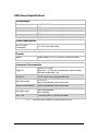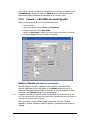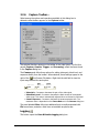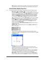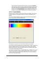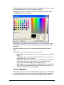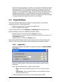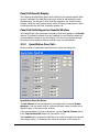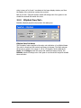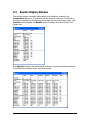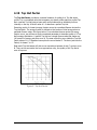
1
LBA-USB/USB-SP User Guide For LBA-USB and LBA-USB-SP Laser Beam Analyzer For Windows XP Professional ® LBA-USB Software Version 4.84 LBA-USB-SP Software Version 4.83 For Sales, Service or Technical Support Phone: (435) 753-3729 Fax: (435) 753-5231 Service Email [email protected] Sales Email [email protected] Ophir-Spiricon Inc. 60 W 1000 N Logan, Utah 84321 © 2008 Ophir-Spiricon Inc. Manual No. 11295-001 Document No. 11294-001 v4.83 Notice Ultracal! is a trademark of Ophir-Spiricon Inc. The Ultracal! processing feature is protected under United States Patent Nos. 5,418,562 and 5,440,338. Windows, Windows XP, Windows Vista, Visual Basic and Excel are registered trademarks of Microsoft Corporation. LabVIEW is a registered trademark of National Instruments. Pentium is registered trademarks of Intel Corporation. All rights to the product and any accompanying user guide(s) are reserved by OphirSpiricon Inc. Ophir-Spiricon Inc. reserves the right to make improvements to the product described in this user guide at any time and without prior notice. While every precaution has been taken in the preparation of this guide, the publisher and author assume no responsibility for errors, omissions, or any loss of data because of said errors or omissions. Personal computer hardware and component manufacturers, along with operating system providers, constantly revise their products and software upon which this product is dependent. While Spiricon, Inc. endeavors to maintain maximum compatibility with a wide variety of personal computer configurations, Spiricon, Inc. makes no guarantee that any one brand or model of personal computer will be compatible with any or all of the features contained in this application, either now or in the future. Obtain the latest version of this user guide at www.ophir-spiricon.com. LBA-USB User Guide Document No: 11294 Page 3 Table of Contents Safety ....................................................................................................................... 8 General Information................................................................................................... 9 Chapter 1. Equipment Setup ............................................................................... 15 1.1 LBA-USB/USB-SP Software Installation ........................................................ 15 1.2 Connect the Camera................................................................................... 15 1.3 Launch LBA-USB/USB-SP ............................................................................ 15 1.4 Select the Camera...................................................................................... 16 1.5 Collect Data ............................................................................................... 16 Chapter 2. Menus and Dialog Boxes .................................................................... 17 2.1 File Menu................................................................................................... 17 2.2 Options Menu ............................................................................................ 31 2.3 Pass/Fail Menu........................................................................................... 78 2.4 Window Menu............................................................................................ 83 2.5 Start! and Stop! Menu Action Items............................................................. 83 2.6 Ultracal! Menu Action Item ......................................................................... 84 Chapter 3. Display Windows................................................................................ 85 3.1 Main Window ............................................................................................. 85 3.2 Beam Display Window ................................................................................ 86 3.3 Results Display Window.............................................................................. 88 3.4 Pan/Zoom Display Window ......................................................................... 89 3.5 Tilt and Rotation Display Window ................................................................ 90 3.6 Histogram Display Window ......................................................................... 91 3.7 Shortcuts................................................................................................... 92 Chapter 4. Computations .................................................................................... 93 4.1 Computational Accuracy ............................................................................. 93 4.2 Numerical Formats ..................................................................................... 93 4.3 Beam Presentation Affects Results .............................................................. 93 4.4 Manual Background Energy Nulling ............................................................. 94 4.5 Clip Level................................................................................................... 95 4.6 Total Energy .............................................................................................. 95 4.7 Percent in Aperture .................................................................................... 96 4.8 Peak and Min ............................................................................................. 96 4.9 Peak Location ............................................................................................ 96 4.10 Centroid Location ....................................................................................... 96 4.11 Beam Widths and Diameters....................................................................... 97 4.12 Elliptical Beam ......................................................................................... 100 4.13 Gauss Fit ................................................................................................. 101 LBA-USB User Guide Document No: 11294 Page 5 4.14 4.15 4.16 4.17 4.18 4.19 4.20 4.21 4.22 4.23 4.24 4.25 4.26 4.27 Chapter 5.1 5.2 5.3 5.4 5.5 Page 6 Whole Beam Fit Equations ........................................................................ 102 X/Y or Major/Minor Line Fit Equations........................................................ 102 Deviation of Fit ........................................................................................ 103 Correlation of Fit ...................................................................................... 104 Top Hat ................................................................................................... 104 Top Hat Factor......................................................................................... 106 Effective Area and Effective Diameter........................................................ 107 Far-Field Divergence Angle Computations .................................................. 107 Histogram................................................................................................ 109 Statistics.................................................................................................. 110 Frame Averaging...................................................................................... 111 Frame Summing....................................................................................... 111 Gamma Correction ................................................................................... 112 Convolution ............................................................................................. 112 5. ActiveX............................................................................................ 115 Introduction............................................................................................. 115 Using ActiveX........................................................................................... 115 Properties, Methods and Events ................................................................ 118 DCOM ..................................................................................................... 130 Resolving Problems .................................................................................. 133 Document No: 11294 LBA-USB User Guide Table of Figures Figure Figure Figure Figure 1 2 3 4 – – – – Hirose Connector Pin-Out Diagram............................................................ 37 Top Hat Factor ...................................................................................... 106 Convolution Processing .......................................................................... 113 Low-Pass Spatial Filter Convolution Coefficients ....................................... 114 LBA-USB User Guide Document No: 11294 Page 7 Safety While the LBA-USB itself does not present the operator with any safety hazards, this instrument however is intended for use with laser systems. Therefore, the operator should be protected from any hazards that the laser system may present. The greatest hazards associated with laser systems are damage to the eyes and skin due to laser radiation. Optical Radiation Hazards With almost any camera used with LBA-USB, the optical radiation at the camera sensor is low enough to be considered relatively harmless. Nevertheless, use of this instrument may require the operator to work within the optical path of lasers. Exposure to radiation from these lasers may be sufficient to warrant the use of protective equipment. Unless the laser’s optical path is enclosed, the operator should be protected against accidental exposure. Exposure to personnel other than the operator must also be considered. Hazards include direct beam exposure and reflected radiation. When working with an unenclosed beam path, it is advisable to do so while the laser is powered down or at reduced power levels. Whenever there is a risk for dangerous exposure, protective eye shields and clothing should be worn. Electrical Hazards The cameras used with LBA-USB utilize only low voltages, derived from the USB port in the host PC computer, therefore it posses no risk of electrical shock. The computer should always be operated with its covers in place and in accordance with its manufacture’s recommendations. The computer should always be operated with a properly grounded AC power cord. Page 8 Document No: 11294 LBA-USB User Guide General Information Introduction This manual covers the operation of LBA-USB and LBA-USB-SP products. In some places the two products are shown as LBA-USB/USB-SP to indicate that the material applies equally to both products. In some cases only the abbreviated LBA-USB will be used, but the USB-SP version is implied. Where only one or the other is covered the text will indicate which version is applicable. The primary difference is that LBA-USB operates with the Lxxxxx camera types while LBAUSB-SP operates with the SPxxx camera types. The Spiricon Laser Beam Analyzer Model LBA-USB/USB-SP, is a low cost, PCbased product for use in modern Pentium-generation personal computers with a USB2 interface. It provides all the essential features needed for laser beam analysis. Some of these features include: High-speed high-resolution false color beam intensity profile displays in both 2D and 3D Operates in Windows XP Professional, or higher operating systems Numerical beam profile analysis employing advanced patented calibration algorithms User selectable choices for making beam width measurement, including Second Moment methods Pass/fail testing available on most measured parameters Both Whole beam and Linear Gaussian fits to beam data Top Hat measurements based on the beam profile or a user defined area or line Signal-to-noise ratio improvement through averaging and background subtraction Frame summing for cumulative effect analysis Statistical Analysis of all measured parameters Beam Stability analysis Histogram display and results Post processing capabilities Both Drawn and Auto Aperture for isolating beam data Both Results and Data logging capabilities Flexible printing options for hard copy generation Two Divergence measurement techniques LBA-USB User Guide Document No: 11294 Page 9 A complete LBA-USB/USB-SP systems consists of the following equipment: The Spiricon LBA-USB/USB-SP software An L070, L130, L230, L11058, SP503, or SP620 camera and USB cable A Pentium style or compatible PC with: • USB 2.0 interface, either built into the computer or motherboard, or installed via PCI card • Pentium, Pentium Dual/Quad core or equivalent processor based motherboard • Graphics accelerator card (support for 1024 x 768 minimum) • At least 1GB of main memory, 2GB recommended • At least 15 MB of hard disk space available, much more (>1 GB) to log data files • A high-resolution color monitor • Windows XP-32 Professional or Vista 32 operating system • A CD-ROM Drive Optional equipment: USB 2.0 PCI interface card A printer with appropriate Windows compatible drivers LBS-100, BA-VIS, -NIR, or -BB Laser Beam Attenuator Most laser beam energy requires attenuation before application to the camera sensor. Attenuation requirements vary greatly depending upon application. Spiricon offers optional equipment for beam attenuation. Consult your Spiricon Representative or call the Spiricon's Sales Department for further information. Page 10 Document No: 11294 LBA-USB User Guide USB Camera Specifications Environmental Storage Temperature -10° C to 60° C Storage Humidity 95% maximum (non-condensing) Operating Temperature 0° C to 50° C Operating Humidity 95% maximum (non-condensing) Power Requirements USB 2.0 Power Consumption ~2.5 W, varies with model Physical Weight Approximately 312 g (11 ounces), varies with model Instrument Characteristics Trigger In Rising LVTTL input Max input +3.3 Vdc with programmable exposure delay Minimum pulse width 1 µs Strobe Out LVTTL output with programmable delay Video Gain Adjust 1 to 23 dB User programmable, varies with model Shutter Control Outputs User programmable, varies with model Video Black Level User programmable Set by Ultracal RMS – S/N ~60 dB @ Gain 1.4, varies with model Note: All specifications subject to change without notice. LBA-USB User Guide Document No: 11294 Page 11 Instrument Characteristics USB L070 1/3” Format Spectral Response USB L130 ½” Format 190 – 1100 nm USB L230 1/1.8” Format 190 – 1320 nm Maximum Beam Size 4.7 x 3.6 mm 6.5 x 4.8 mm 7.1 x 5.4 Pixel Spacing 7.40 μm x 7.40 μm 4.65 μm x 4.65 μm 4.40 μm x 4.40 μm Number of Effective Pixels 640 x 480 1392 x 1040 1616 x 1216 Minimum System Dynamic Range 61 dB 59 dB 59 dB Spatial Uniformity ±0.5% Frame Rate 60 fps at full resolution 100+ fps 320 x 240 15 fps at full resolution 30 fps at 640 x 480 12 fps at full resolution 30 fps at smaller ROI Photodiode Trigger Optional photodiode trigger available: ESP-STC P/N SP90033 Lowest Measurable Signal 1.14 nW/cm2 .63 nW/cm2 1.1 nW/cm2 Saturation Intensity 1.1 μW/cm² 0.5 μW/cm² 0.9 μW/cm² Damage Threshold 0.15 mW/cm2 Operation Mode Interline transfer progressive scan CCD PC Interface USB 2.0 Note: All specifications subject to change without notice. Instrument Characteristics USB L11058 35mm Format Spectral Response 250-1100 USB SP503U ½” Format 190 – 1320 nm USB SP620U 1/1.8” Format 190 – 1320 nm Maximum Beam Size 20 x 13.5 mm 6.5 x 4.8 mm 7.1 x 5.4 Pixel Spacing 9.9 μm x 9.9 μm 4.65 μm x 4.65 μm 4.40 μm x 4.40 μm Number of Effective Pixels 4006 x 2672 1392 x 1040 1600 x 1200 Minimum System Dynamic Range 59 dB 63 dB 60 dB Spatial Uniformity ±0.5% Frame Rate 3.5 fps at full resolution, higher rates with binning & smaller ROI 30 fps at full resolution 8.3 fps at full resolution Photodiode Trigger N/A Optional photodiode trigger available: P/N SPZ17005 Lowest Measurable Signal TBD nW/cm2 .5 nW/cm2 2.5 nW/cm2 Saturation Intensity TBD μW/cm² 1.3 μW/cm² 2.2 μW/cm² Damage Threshold 0.15 mW/cm2 Operation Mode Interline transfer progressive scan CCD PC Interface USB 2.0 Note: All specifications subject to change without notice. LBA-USB User Guide Document No: 11294 Page 13 How to Use This User Guide Read this user guide before setting up the LBA-USB system. Become familiar with the laser beam analysis theory and acquire a basic understanding of how LBA-USB operates. Insights gained through this review will greatly assist you when operating LBA-USB, performing system configurations, and interpreting LBA results. Chapter 1 provides set up instructions contains general operating procedures. Chapter 2 describes all the various menus and dialog boxes in detail, along with configuration considerations and optimization techniques. Chapter 3 explains the beam display and results windows. Chapter 4 presents background information on the theory behind the laser beam measurements and the ISO measurement methods, as well as the calculations embedded in the LBA-USB system. Chapter 5 presents instructions on how to use the ActiveX-based LBA-USB Automation Server. Chapter 1. Equipment Setup Install the LBA-USB/USB-SP application Connect the camera Launch LBA-USB/USB-SP Configure LBA-USB/USB-SP for your camera Collect data 1.1 LBA-USB/USB-SP Software Installation Important: Do not connect the camera to the computer until after the LBA-USB software is installed. 1. Start Windows. 2. Close all other applications. 3. Place the Spiricon CD into your CD-ROM drive. 4. Windows XP will open a dialog that asks: “What do you want Windows to do?” 5. Select “Open folder to view files.” A window will open to display the CD’s root directory containing folders for each of the available Spiricon applications. 6. Open the LBA-USB/USB-SP folder. 7. Double-click the Setup.exe file to launch the installation. 8. Follow the directions provided by the InstallShield Wizard dialog boxes. 9. LBA-USB should now be installed. 1.2 Connect the Camera With the included USB cable, connect the camera to the PC’s USB port. Windows will detect the new hardware and install the necessary software drivers. 1.3 Launch LBA-USB/USB-SP To start the Laser Beam Analyzer USB application, go to the Windows taskbar and select Start > All Programs > Spiricon > LBA-USB/USB-SP > LBA-USB/USB-SP Important: Review the remaining chapters of this user guide and become familiar with the operation and capabilities of the LBA-USB system before performing any laser measurements. LBA-USB User Guide Document No: 11294 Page 15 1.4 Select the Camera The first time LBA-USB starts you will be required to select a startup configuration file. Select the configuration file that corresponds to the model number of the connected camera. Note: This file name has now become the new default configuration file. This default will remain from one session to the next until a new configuration file is saved or restored. The last loaded or saved configuration becomes the startup default. The camera indicator at the bottom of the application window should be green, indicating the camera has been selected and is active. You may now collect data. 1.5 Collect Data To begin collecting data from the camera, click the Start! menu item. The frame display window should immediately start changing colors corresponding to the intensity of the light reaching the camera sensor. The two beam profile displays should also change from a flat line to a curve indicating the light intensity at the cursors. If the room lighting is sufficiently bright and/or the camera is sensitive enough, the frame display window may be entirely white as the horizontal and vertical profile displays move upward and to the right, respectively. If this is the case, reduce the amount of light reaching the camera sensor by shading it with your hand. By manipulating the amount of light reaching the sensor, the entire range of colors (shown on the color bar along the right side of the display window) should be visible in the display window. If the camera has a lens, adjust the lens f-stop and focus to obtain a recognizable image. Caution: Before exposing the camera to a laser beam, make sure that the power/energy of your laser is well below the damage threshold of the camera’s photo imager. Furthermore, the beam may also require attenuation in order to bring it into a range below sensor saturation. Page 16 Document No: 11294 LBA-USB User Guide Chapter 2. Menus and Dialog Boxes 2.1 File Menu 2.1.1 Load… A saved data file can be loaded into the frame buffer for display and results processing. The native file extension denoting a data file created by LBA-USB is “.usb-data”. If the saved file was generated using Ultracal! processing, then the results obtained when loading and viewing this file type are of high quality. Data files can contain one or more frames of data. Each frame of data is called a Record. Embedded in each Record is all the information necessary to accurately reproduce the original frame. Pixel scale, Camera information, energy and Ultracal! values etc. are saved within each Record. Important: File compatibility with new versions of LBA-USB software: We will make every effort to make all future releases of LBA-USB application backwards compatible with all prior data file formats. However, we cannot guarantee that new versions will produce files that will be backward compatible with older versions. Load Data From a File Enter the drive:\paths\<filename>.usb-data of the desired data file. Press Browse... to locate the file via Windows Explorer. If the file contains multiple records and only a subset of the total are desired, enter the beginning record in the Start Record field, followed by a quantity in the Number of Records field. An entry of 0 will load all the remaining records in the file. Records can only be loaded sequentially from the Start Record position. If a quantity of records greater than the space available in the frame buffer is specified, then the frame loading process will fill the remaining buffer and then LBA-USB User Guide Document No: 11294 Page 17 wrap around to the beginning, leaving the last records transferred in the frame buffer. See the Frame Buffer Size paragraph in section 0. In the Start Frame field, enter the location in the frame buffer to begin depositing the file records. Multiple frames will load from that location upward, skipping any locations that are write-protected. Special Frame Numbers The following Frame numbers have special meanings; however they can be saved and loaded in the manner described above. Frame 0 is the Reference Frame Frame -1 is the Gain Correction frame. It is not a true image frame, but rather an array of gain correction factors. Load Files From Windows Explorer Load frame data files from Windows Explorer by dragging and dropping one or more files to the LBA-USB application. Alternately, double-click the data file name to open it. Double-clicking a data file will also start the application if it is not already running. These Windows Explorer shortcuts will work on all frame data formats. However, the current camera configuration must match the configuration of the desired data file. Furthermore, if a data file contains multiple records, all the frame records will be loaded into the frame buffer up to the maximum size of the buffer. Example: If you drag and drop a file containing 20 records, and your frame buffer size is set to 10 frames, then only the first 10 records in the data file will load. 2.1.2 Save As… Save or append data frames in the frame buffer to a file for future reference. All data files saved by the LBA-USB application include a .usb-data file name extension. Data files can contain one or more frames of data. Each frame of data is called a Record. All the information necessary to accurately reproduce the original frame remains embedded in each record: pixel scale, camera information, energy and Ultracal! values, etc. Page 18 Document No: 11294 LBA-USB User Guide Enter the desired drive:\paths\<filename> or select Browse... to locate a file to which frame data will be appended or to overwrite an existing file with data contained in the frame buffer. Enter the Start Frame buffer location from which you want to begin saving or appending frame data files. To append frame data to an existing file, indicate a Start Frame position greater than the last frame contained in the existing file. To save multiple records, enter a value in the Number of Frames field greater than “1” but less than or equal to the total frames in the frame buffer. Enter a value of “0” to include all the frames in the frame buffer. Multiple data frames can only be saved sequentially from the Start Frame location. 2.1.3 Export Image Exporting an image provides single data and pixel images for use in other applications. Keep in mind that exported images cannot be reloaded into the LBA-USB application. (To export a series of images to a log file, see section 2.1.11). The BMP (bitmap) option, for example, simply provides a picture of the beam image and does not represent a viable data source for numerical analysis. Bitmap images will appear in external applications just as the current beam display window image appears. To perform external computations on exported data, only the two ASCII formats provide a viable method for doing so. ASCII file types are available in either comma (.CMA) or space (.SPA) delimited formats. Spreadsheet programs like Excel typically use comma-delimited data, while math programs like MathCAD typically use a space-delimited format. Consult the external application’s documentation to determine which style to use. 1D beam display images, defined by the location of the Horizontal and Vertical Cursors are also available for export. Cursor files are designated with a .CUR file type. Cursor files are in ASCII and delimited by a comma. The cursor image contains Horizontal data first and then left to right, followed by a carriage return, and then provides the Vertical data, top to bottom. A Column and Row summed beam image is defined by the total of all pixel values summed in both the horizontal and the vertical direction. Column/Row summed files are designated with a .SUM file type. Summed files are in ASCII LBA-USB User Guide Document No: 11294 Page 19 and delimited by a comma. The summed image contains horizontal data first, and then left to right, followed by a carriage return, and then provides the vertical data, top to bottom. Note: Remember, exported image files cannot be read back into the LBA-USB frame buffer. To save retrievable data files, use Save As... and Load... under the File menu. To export an image, enter the desired drive:\paths\<filename>. Select Browse... to locate an existing file or to overwrite an existing file. Enter the Start Frame buffer location from which you want to begin exporting image data files. To save multiple images, enter a value in the Number of Frames field greater than “1” but less than or equal to the total frames in the frame buffer. Enter a value of “0” to export all of the frames in the frame buffer. Multiple export images can only be saved sequentially from the Start Frame location. When exporting multiple images, each image will be placed into a separate file. The file name will automatically include a six-digit number appended to the entered file name. This is a sequential number starting at 000000. Thus, a given multiple image export would create a series of files that will appear as: <filename>000000.cma;<filename>000001.cma;...<filename>NNNNNN.cma Select the image file Export Format (or Formats) desired for the export. 2.1.4 Save Config… The current LBA-USB setup configuration can be saved to a file for later restoration. All configuration files include the .usb-cfg file extension. Multiple configuration files may be saved for multiple setups. Whichever configuration was last saved (or restored), becomes the default configuration loaded the next time the LBA-USB application is launched. The configuration file includes all setup parameters within the LBA-USB menus. Page 20 Document No: 11294 LBA-USB User Guide The saved configuration file does not include, and thus will not restore data frames, reference frames, gain correction frames, or Ultracal! processing information. These types of frames must be saved and restored separately. Note: Remember to perform an Ultracal! cycle immediately prior to acquiring new data frames. Since camera calibration, equipment setup and operating conditions can vary between sessions and even during extended sessions, performing frequent Ultracal! cycles ensures the highest level of reliable data acquisition. 2.1.5 Restore Config… LBA-USB setup configurations may be restored from previously saved .usb-cfg files. Whichever configuration was the last to be restored (or saved), will become the default configuration the next time the LBA-USB application is launched. The configuration file includes all setup parameters within the LBA-USB menus. The saved configuration file does not preserve, and thus will not restore Data frames, Reference frames, Gain Correction frames, or Ultracal! processing information. These types of frames must be saved and restored separately. Perform an Ultracal! cycle immediately prior to acquiring new data frames. Since camera calibration, equipment setup and operating conditions can vary between sessions and even during extended sessions, performing frequent Ultracal! cycles ensures the highest level of reliable data acquisition. Note: Restoring a configuration does not change any camera settings; it simply restores the Camera dialog box settings just as they were when the configuration file was created. 2.1.6 Set Reference This feature is also available as a button on the toolbar: Set Reference copies the current frame or the Gauss fit results of the current frame to the reference frame buffer. The reference frame is located at frame number 0 (zero), in the frame buffer. View the reference frame by entering a “0” in the Frame indicator/edit control: Note: The reference frame 0 does not cycle through using the Frame spin controls. The Set Reference Source item located in the Capture dialog box determines the style of the save reference data. LBA-USB User Guide Document No: 11294 Page 21 2.1.7 Generate Gain Generate Gain initiates an automatic Gain Correction calculation cycle. The cycle generates results stored in a gain correction table that will then be used to preprocess all data frames newly acquired from the camera. The gain correction enunciator is located at the bottom of the LBA-USB’s main display screen. If the color of the gain correction enunciator is: GRAY GREEN RED The gain correction processing is turned OFF. The gain correction calculation succeeded and is operating. The gain correction processing has been disabled due to a change in the camera settings (brightness, gain, shutter, frame size/ROI, or bits per pixel) since the gain frame was first captured. How to Generate Gain Before selecting Generate Gain perform the following: Allow the camera to warm up to a normal operating temperature. Align the laser beam with the camera and set the correct settings for Zoom, Pan Camera type, resolution, etc. Block all light from the detector and perform an Ultracal!. Uniformly illuminate the camera detector to an intensity level that is between 60% and 90% of saturation. Next, select Generate Gain from the File menu: After a few seconds, observe that the Gain Correction enunciator turns green. Remove the uniform illumination and re-apply the laser beam to the camera. Note: Perform a Save Config... and a Save Gain As... operation in conjunction with each Generate Gain... operation. This will ensure that when configuration settings are restored, the configuration will allow the gain correction to operate correctly. What is Gain Correction? The gain correction algorithm computes a mean pixel intensity value, and then supplies a correction factor for each pixel that will adjust it to the computed mean. If your camera has dead or seriously defective elements, do not attempt to use or operate the camera with Gain Correction. Page 22 Document No: 11294 LBA-USB User Guide What Disables Gain Correction? Gain Correction becomes disabled if certain data collection conditions change from when the Generate Gain operation was first executed. In all cases, these conditions are the result of an operator’s change to the spatial acquisition settings. The disabled condition will occur if changes are made to: The camera or pixel format The size or location of the custom image The lens setting Brightness Gain Shutter 2.1.8 Load Gain… Restore a previously saved gain correction table from a file. The gain correction enunciator will turn GREEN if the loaded file will operate under the current setup conditions. If it cannot operate under the current setup conditions, it will appear RED. Note: Perform a Restore Config... using a .usb-cfg configuration file that was saved at the same time that the .gai gain correction file was created. This will insure that restored configuration settings will allow the gain correction to operate correctly. 2.1.9 Save Gain As… Save the current gain correction table to a file. All gain correction files include a .gai file name extension. The gain correction table must be generated (see section 2.1.7) prior to saving the table to a file. Note: Perform a Save Config... and a Save Gain As... operation in conjunction with each Generate Gain... operation. This will ensure that restored configuration settings will allow the gain correction to operate correctly. 2.1.10 Gain On/Off This feature is only available as a button on the toolbar: Click on this button to toggle gain correction processing off or on. This feature will only operate once a gain correction table is present. To generate a gain correction table, perform the steps found in section 2.1.7 or load a previously generated gain table (see section 2.1.8). LBA-USB User Guide Document No: 11294 Page 23 2.1.11 Logging… This feature is also available as a button on the toolbar: Using the LBA-USB’s data logging capability, save any of the following to a file: Frame data Numerical results Export log Frame data log filenames include a .usb-data file extension. A frame data log file may be read back into the frame buffer by using the File and Load... menu selections. Numerical results log filenames include an .RLG file extension. Results log files contain exported numerical results for use with other applications, such as spreadsheets or math programs. These can also be viewed with a common text editor. Results log files are in ASCII format. Export log files can be saved as any of four different types: Bitmap (.BMP), ASCII comma-delimited (.CMA), ASCII space delimited (.SPA), and Cursor data (.CUR). Export log files are write-only. These files are created for use in other applications like spreadsheets or math programs. Unlike frame data logging, export logging creates multiple files rather than one large concatenated file with multiple records. The filename will automatically include a six-digit number appended to the entered file name. This is a sequential number starting at 000000. Thus, an export logging operation would create a series of files that will appear as: <filename>000000.cma; <filename>000001.cma; … <filename>NNNNNN.cma Page 24 Document No: 11294 LBA-USB User Guide Data, Results & Export Logging Dialog Box Select a Logging Type: To log frames of data, check the Data Logging box and enter the desired drive:\paths\<filename> or click Browse… to locate a file, or to append or overwrite an existing file. To log computed results, check the Results Logging box and enter the desired drive:\paths\<filename> or click Browse… to locate a file, or to append or overwrite an existing file. Select the appropriate Format (Spreadsheet or Math Program) required by the external application. Both formats produce a commadelimited ASCII text file. The Spreadsheet format precedes the log with a single list of column headings. The Math Program format precedes each log entry with a binary number that indicates which results are enabled. To log frames of image data, check the Export Logging box and enter the desired drive:\paths\<filename> or click Browse… to locate a file, or to append or overwrite an existing file. Select an appropriate Format required by the external application. The .BMP format produces bitmapped image files. The .SPA format produces an ASCII text image file with space-delimited entries. The .CMA format produces an ASCII text image file with comma-delimited entries. The .CUR format logs only the Cursor image in ASCII format with comma-delimited entries. The .SUM format logs only Column/Row summed data in an ASCII format with comma-delimited entries. See section 2.1.3 for more information regarding these file types. Note: Up to all three logging types may be selected. Select the Logging Method: Continuous – Logging will commence when Start! is clicked and will terminate when Stop! is clicked, or available disk space fills up. Frames – Limit the logging process to a specified Number of Frames. When this option is selected, enter the number of frames to log. Logging will commence when Start! is clicked and will terminate when the specified number LBA-USB User Guide Document No: 11294 Page 25 of frames accrues. Press Stop! to terminate the log early. The Rate display will indicate the number of frames remaining: Time – Limit the logging process to a specified amount of time. When this option is selected, enter the amount of time during which the log will run. Double-click inside the entry item and enter the time value in the format shown. Logging will commence when Start! is clicked and will terminate when the time remaining expires. The Rate display will indicate the amount of time remaining: Select a Pass/Fail Filter: Filter out certain frames of data from appending to the log file by using the Pass/Fail Filter. This must be selected in conjunction with the entries made in one or more of the Pass/Fail menu items (see section 2.3 for more details on how to use the Pass/Fail options.). Example: To only log frames that exceeded a certain minimum amount of energy, select Passed Frames Only. Then, check the Minimum box in the Quantitative Pass/Fail dialog box (under Total Energy). Enter the minimum value of the energy that is required to pass this filter. Begin and Terminate Logging To begin logging to a file, open the select Logging… from the File menu, then within the Data, Results & Export Logging dialog box: Select a logging type Enter a file name Click OK Click Start! on the menu To terminate logging to a file, click Stop!, then: Return to the Data, Results & Export Logging dialog box Uncheck the logging type Click OK Example: If a log was setup to capture 1000 frames, but manually stopped at frame 521, followed again by a restart, the logging process would proceed to the designated frame quantity, completing a log file that contains entries for 1,521 frames. Important: Once a logging cycle begins, each file entry is sequentially recorded until the log is terminated. If a log is stopped, and then restarted, the new entries will continue to be added as before. However, the Frame counter or the Timer (whichever might apply) will reset to 0 (zero) each time Start! is pressed. In Export Logging, the file frame numbering does not reset, but rather continues to increment from the last number assigned. This number is only reset each time logging is enabled. Page 26 Document No: 11294 LBA-USB User Guide How fast will logging operate? The rate at which frames can be processed and logged to a file depends upon such variables as the: Quantity and types of calculations being performed Type of logging enabled Speed of your disk drive and computer system, etc. We recommend running tests to determine how fast your system can log various forms of data and results, and then using this information as your system benchmarks. 2.1.12 Implications of Combining Logging, Statistics, Post Processing and Block Capture Note: Before applying the concepts in this topic become familiar with the operating modes available for: • • • • Results Logging - Section 2.1.11 Statistics Results – Statistics paragraph in Section 2.2.7 Post Processing – Processing paragraphs in Section 2.2.4 Block Capture - Section 2.2.4 The Logging, Statistics, Post Processing and Block Capture features each contain built in controls that can limit their respective run lengths. Operator intervention, a programmed number of frames, or a programmed time limit may introduce these limiting factors. Note: Post Processing and Block Capture do not allow for a programmed time limit. In addition, Post Processing and Block Capture are mutually exclusive. Due to the flexibility in setting control options, it is possible to set conflicting control parameters. Therefore, it is essential that these various conflicts be resolved by a prioritized control scheme. Certainly a perceptive operator can avoid all of these possible conflicts; nevertheless, owing to the complexity of these features, setup errors almost always occur. Therefore, to avoid a conflict in the above features, never set more than one of the above to use either a Time limit or a Frame count, at any one time. Using Logging, Statistics and Block Mode in Combination The following control priorities are in effect when any of the above features are used in combination. The first enabled feature in the list has control. 1. Block Mode – Controlled by a set number of frames. 2. Data or Results Logging – Controlled by a set time limit. 3. Data or Results Logging – Controlled by a set number of frames. 4. Statistics Results – Controlled by a set time limit. LBA-USB User Guide Document No: 11294 Page 27 5. Statistics Results – Controlled by a set number of frames. If Results Logging and Statistics are both in play, and if one of the Logging features is in control, then statistics results are recorded into the results log file when the logging operation terminates. See Begin and Terminate Logging in section 2.1.11. If Results Logging and Statistics are both in play, and if one of the Statistics features is in control, then statistics results are recorded into the results log file whenever the statistics collection cycle completes. Using Logging, Statistics and Post Processing in Combination The following control priorities are in effect when any of the above features are used in combination. The first enabled feature in the list has control. 1. Post Processing – Controlled by a set number of records/frames unless the number is set to zero. (Note: Set this number to zero to allow the Logging and Statistics operation to operate on multiple records from multiple files.) 2. Data or Results Logging – Controlled by a set number of frames. 3. Statistics Results – Controlled by a set number of frames. Important: No timed operations are recognized when Post Processing is enabled. If Results Logging and Statistics are both in play, and if the Logging feature is in control, then statistics results are recorded into the results log file when the logging operation is terminates. See Begin and Terminate Logging in section 2.1.11. If Results Logging and Statistics are both in play, and if the Statistics feature is in control, then the statistics results are recorded into the results log file when the statistics collection cycle completes. Page 28 Document No: 11294 LBA-USB User Guide 2.1.13 Print… Select the information to be sent to the printer within the Print dialog box. Open this dialog box via the File menu. Note: Simply clicking on the print toolbar button immediately produces output based on the last configuration set in the Print dialog box. Check the Beam Image box to print the contents of the beam display window. The printed image contains everything visible in the window, limited only by the resolution and color capabilities of your printer and Windows printer driver. Check the Results box to print the results information. The printed results consist of all enabled numerical results including Statistics and Histogram. Note: For both of the above options, if the related child window (Beam, Results, or Histogram) is minimized, then the associated item will not be printed. In other words, “what you see is what you get.” If both Beam Image and Results are checked, then the beam image will appear first followed by the results set. If the Separate Pages box is checked, then the beam image and results set will be printed on separate pages. Check the Current Frame Only box to only print the currently displayed frame and/or its results. If this box is not checked, direct LBA-USB to print multiple frames by specifying the From Start Frame location, and the Number of Frames to print. The Number of Frames can be set to 0 (indicates all the frames in the buffer), or from 1 to the maximum number of frames in the frame buffer. When printing multiple frames, observe that LBA-USB cycles through the designated frame locations. It computes the required results for each frame and then prints whatever is required. At the end of this process, the last frame printed and its results appear on the display. LBA-USB User Guide Document No: 11294 Page 29 If Statistics results are enabled: These will not update during the printing operation and thus will show the same values on each frame’s printout. Note: To avoid unnecessary printing, keep the Current Frame Only box checked unless multiple frames are absolutely required. When printing 2D beam images, in either 128 or 16 colors, the dark violet background color converts to a shade of light gray. This may not always be appropriate, as the dark background may prove useful for transparencies, etc. To restore the normal background appearance, enable the 2D Dark Background. 2.1.14 Print Setup… This is the standard Windows style Print Setup dialog box. Select which printer to use, and make some basic print format choices. Your specific printer’s Options dialog box may also be accessible, offering other selections that pertain to your particular printer. 2.1.15 Exit Click on Exit from the File menu to leave the LBA-USB application and return to the Windows desktop. This ends the current beam analysis session. Before exiting, consider the following questions: Do you want to save the current setup to a configuration file? Have you correctly terminated any logging files? Do you need to save any frame data files? Do you need to save any important Reference frame data? Do you need to save a Gain Correction table for future use? Page 30 Document No: 11294 LBA-USB User Guide 2.2 Options Menu 2.2.1 Show/Hide the Capture, Display and Aperture Toolbars These three toolbars can be alternately displayed or hidden based on operator preference. The Capture and Display toolbars can be modified to match the operator’s needs. The Aperture toolbar is predefined and cannot be modified by the operator. 2.2.2 Aperture… LBA-USB can display three types of apertures in four different shapes. Three types of apertures Drawn – Manually draw a WHITE aperture for the purpose of isolating beam analysis to the pixel data contained within the aperture. This feature allows the elimination of the effects of noise or stray energy in regions outside of the beam under test. Displayed – The BLACK displayed aperture is not really an aperture; it is an overlaid graphical representation of the computed shape and size of the beam width/diameter results. This BLACK aperture provides a way for the user to visually see the beam width, and observe how it changes. Auto – This feature automates the task of drawing an optimally sized and placed aperture around the beam profile being measured. This aperture is displayed in YELLOW. It performs the same function as the Drawn aperture, except that it continuously resizes itself to changing beam conditions. All three of the above apertures can be enabled and visible at the same time on a 2D display. In the 3D display mode, no apertures are ever displayed. However, the Drawn and Auto apertures can be operating as described above. If the apertures are enabled while in the 3D display mode, be sure to check their setup in the 2D display mode. The Drawn and Auto apertures, when operating at the same time, function in the following manner: 1. The Drawn aperture isolates the energy for analysis. 2. An Auto Aperture is computed and drawn around the beam energy. 3. The reported beam widths/diameter is computed based on the energy contained exclusively within the Auto Aperture. Aperture Shapes LBA-USB User Guide Document No: 11294 Page 31 Drawn and Displayed apertures can be rendered in four shapes: Circle Square Ellipse Rectangle Auto apertures are always rendered as an ellipse. How to Create a Drawn Aperture Create a drawn (or manual) aperture by using the Aperture dialog box, the Aperture toolbar, or by dragging and dropping the aperture in the 2D display window. Note: Before using the drag and drop method, first select a drawn aperture shape using either of the first two methods. The Aperture dialog box, and the Aperture toolbar offer the same choices for creating a drawn aperture. The entries that define a Drawn aperture are listed vertically within the recessed panel of the dialog box. These same entries are arranged horizontally on the aperture toolbar. The same selections can be made from either location. The following discussion references the dialog box, but applies equally to the toolbar. 1. Select an aperture Shape. 2. Enter the aperture’s Center location in X and Y coordinate values. 3. If the aperture is an ellipse or rectangle, enter the Size of the Major and Minor axes, followed by the Rotation angle of the Major axis in degrees. 4. If the aperture is a circle or square, enter the Diameter (not shown above). Page 32 Document No: 11294 LBA-USB User Guide Drag and Drop Apertures Once a Drawn aperture is enabled from either the dialog box or toolbar, move, resize, and (in the case of an ellipse or rectangle) rotate it. Move the arrow cursor over the display window and press and hold down the right mouse button. This reveals the Drag, Drop and Rotate hot spots of the Drawn aperture. Move the arrow cursor onto one of these hot spots, release the RIGHT mouse button and press and hold down the LEFT button. The cursor changes shape indicating the selected Drag and Drop function. Now drag the mouse to see what happens to the aperture. The four cursor styles perform the following operations: Moves the aperture center. Sizes the aperture right or left. Sizes the aperture up or down. Rotates an elliptical or rectangular aperture. Using Auto Apertures To enable the Auto aperture feature, click on the Use Auto Aperture box, or click on the Auto aperture button on the Aperture toolbar. Consider the following when using Auto apertures: Auto apertures are drawn in YELLOW, appear as ellipses, and are only visible on 2D displays. Auto apertures will be drawn on the X and Y-axes of the beam if Elliptical is off, and on the Major and Minor axes of the beam if Elliptical is on. Always enable Auto apertures whenever performing second moment D 4-Sigma beam width measurements. If your beam is small, relative to the acquisition window size, either use a Drawn aperture of 2x to 2.5x the beam width, or enable Auto aperturing to perform this task for you. Auto apertures help improve beam measurement accuracy on almost any beam shape. However, Auto apertures may not improve accuracy, or operate well, if a considerable amount of stray energy is present adjacent to the beam profile. In this case, rely on a well-placed Drawn aperture, and avoid using the D 4-sigma beam width method. Display Beam Width To see the beam widths and diameter graphically overlaid on the laser beam profile, select the shape that most correctly matches your beam. These choices are also available from the Aperture toolbar. The displayed beam widths appear as a BLACK aperture in a 2D beam display window. This aperture does not appear in 3D displays. LBA-USB User Guide Document No: 11294 Page 33 If the beam is an off axis ellipse or rectangle, be sure to turn on Elliptical in the Computations... dialog box under the Options menu. Otherwise all drawn beam widths will be computed and displayed on the X and Y-axes. 2.2.3 Camera…, LBA-USB-Lxxx model specific Make the following selections in the Camera dialog box: Select a Camera Select the required camera Format and Frame Rate Determine the size of the Frame Buffer Modify the Pixel Scale if needed (the native camera pixel scale is the default) Choose the Lens mode if the camera is so equipped Select a Camera (LBA-USB-Lxxx model specific) Any USB camera currently connected to your computer while LBA-USB is running, regardless of port, will appear in the Camera drop-down list. If a camera is connected after the dialog is displayed, it may be necessary to close and reopen the Camera dialog box to refresh the list. Note: A camera disconnected after LBA-USB has launched will remain active on the list. The green/red icon located on the status bar indicates whether the camera is currently connected to the computer. Only one instance of LBA-USB can select a camera at one time. Cameras selected by another instance of LBA-USB appear in parentheses and cannot be selected. Page 34 Document No: 11294 LBA-USB User Guide Select the desired camera from the list in the Camera field. If the desired camera does not appear: Verify that the camera is connected to the computer. Verify that the camera has power. (For example, the green LED on the side of the USB camera should be lit.) Try resetting the camera. Disconnect the USB cable, wait 10 seconds, and plug it in again. Close and reopen the Camera dialog box to refresh the list. Contact the Spiricon Service Department for assistance. If your camera is surrounded by parentheses and cannot be selected: The camera is currently selected by another instance of LBA-USB running in the same computer. Cameras can only be selected by one LBA-USB instance at one time. Select a different camera in the other instance of LBA-USB, then close and reopen the Camera dialog box. The camera should now be available for selection. Contact the Spiricon Service Department for assistance. If your camera is surrounded by brackets and cannot be selected: The camera has not been licensed for use with LBA-USB. Contact the Spiricon Service Department for assistance. Format and Frame Rate (LBA-USB-Lxxx model specific) Select from a list of predetermined formats or establish a custom region of interest. Each selection defines a fixed set of offsets, widths and heights, along with the optimal resolution for that format. These characteristics cannot be changed by the user (unless a Custom ROI is selected – see below). The available Frame Rate settings (in Hertz) are determined by the size of the region, the pixel format, and the packet size (speed). The selected rate is displayed in the bottom status bar of the LBA-USB display. Sampling and Binning (LBA-USB-Lxxx model specific) Those formats that include a sample parameter (2x2 sample, for example) restrict data acquisition to only the top left pixel of each pixel group. Those formats that include a binning parameter (2x2 binning, for example) accumulate the values of each pixel in the group. LBA-USB User Guide Document No: 11294 Page 35 Set a Custom ROI (Region of Interest) (LBA-USB-Lxxx model specific) Select this Format option to either further reduce the amount of data collected (thus allowing for faster frame capture rates) or to focus in on a specific region of interest. The format x and y Offsets and Width/Height settings from the previous selection are retained as the starting point for the custom ROI. To set a custom ROI, modify the x and y Offsets to establish the new location of the top left pixel of the ROI. Next, define the size of the ROI in pixels by Width and Height. Finally, select an appropriate Frame Rate calculated for the application. The available rates are dependent on the size of the region, the pixel format, and the shutter setting. Note: The Resolution parameter remains fixed at x1. Number of Frames (LBA-USB-Lxxx model specific) The Number of Frames or Size, Kb setting determines the buffer size, or the total amount of system memory allocated to the temporary storage of digitized video frames. There are two ways to set frame buffer size. Enter a specific amount of memory to allocate in the Size, Kb field Specify the Number of Frames available to the buffer We recommend setting the number of Frames, rather than the amount of memory allocated to the Buffer Size. What is the Frame Buffer? The frame buffer is an allocated block of the PC’s system memory. It receives and temporarily retains frames of digitized video data. The frames in the frame buffer are numbered from 1 to N, where N is the maximum number of frames allocated. At least one frame must be allocated in the frame buffer. The frame buffer is loaded in a sequential round robin fashion. Frames of data can be placed into the frame buffer by: Transferring data from a digital camera Loading data from a file Post processing data already in the frame buffer Post processing data from a file In the far lower right hand corner of the main screen display is a Frame edit and spin control: The number visible in the edit control indicates frame number currently displayed. Edit this number by double-clicking and entering a new value, or use the spin control to increment or decrement to the desired frame. We recommend setting the frame buffer to contain as many frames as your Windows environment allows in real memory. This will prevent LBA-USB from attempting to use virtual memory (hard drive space) as frame buffer space. A Page 36 Document No: 11294 LBA-USB User Guide small amount of virtual memory assigned to the frame buffer is not critical, but a great deal may make you wonder what kind of alien being has just taken over your hard drive. Windows will allocate the frame buffer to real memory first. When it is filled, Windows allocates virtual memory. For this reason, it is a good idea to run LBAUSB with no other applications running in the background. This will free up as much real memory as possible for frame buffer use. How do I know when my frame buffer is spilling into virtual memory? The hard disk drive light will begin to flicker when the real memory frame buffer capacity is filled, and the virtual file swapping begins. To avoid this, reduce the frame buffer size until it stops. Note: Be sure to analyze this occurrence and perform the adjustment with Logging disabled. Pixel Bits (LBA-USB-Lxxx model specific) Select the number of bits to allocate per pixel. External Trigger Input (LBA-USB-Lxxx model specific) An external trigger enables the camera to be synchronized with an external source. Triggers are rising edge sensitive and should only be connected to 3.3V or LVTTL digital logic signal. Higher voltage may cause damage to the camera. The included cable connects to the trigger input on the camera. If an external input trigger is attached to the camera, activate the External Trigger Input option, and then adjust the exposure delay (in milliseconds) as necessary. The exposure delay sets the time interval between the moment when the trigger is received and the moment when the exposure begins. Strobe Out (LBA-USB-Lxxx model specific) Activate the Strobe option to enable the strobe output feature. No cable is supplied for strobe out. The 6-pin Hirose connector houses both the trigger in and strobe out signals. The wiring diagram for a cable connector is shown in the figure below. TRIGGER IN STROBE OUT 6 1 VIDEO SOF GROUND 5 2 4 3 VCC OUTPUT GROUND Figure 1 – Hirose Connector Pin-Out Diagram (Hirose Connector P/N HR10A-7P-6P(73))[not applicable for L11058] Note: This connector also accommodates the optional optical trigger probe (ESP-LUM). LBA-USB User Guide Document No: 11294 Page 37 Adjust the Strobe Delay (in milliseconds) to determine the interval between the moment when the exposure begins and the moment when the strobe output pulse initiates. Pixel Scale and Units Enter a vertical and horizontal Pixel Scale value appropriate for your optical system and camera. The pixel scale value is derived from the camera’s detector specifications, or may be user programmable to correspond to the characteristics of your optical system. For the camera imager based scale setting, the value to enter is the minimum line pitch of the camera’s detector. Select the Pixel Units value that applies to the entered pixel scale value. Camera detector pixel pitch is specified in micrometers (µm). Gamma Correction If the camera employs a solid state CCD or MOS style detector, then its detector responds linearly to monochromatic light. For linearly responding cameras the Gamma setting should be set to 1. Lens Check this box if the camera is fitted with a lens. When enabled, the 2D image orientation is adjusted to depict the image as if the observer is standing and viewing the scene from behind the camera. When disabled, the 2D image is oriented as if the observer is standing in front of the camera looking at the surface of the detector. 2.2.4 Camera…, LBA-USB-SP specific Make the following selections in the Camera dialog box: Select a Camera Select the required camera Format and Frame Rate Determine the size of the Frame Buffer Modify the Pixel Scale if needed (the native camera pixel scale is the default) Choose the Lens mode if the camera is so equipped Page 38 Document No: 11294 LBA-USB User Guide Select a Camera (LBA-USB-SP specific) Any USB-SP style camera currently connected to your computer while LBA-USBSP is running, regardless of port, will appear in the Camera drop-down list. If a camera is connected after the dialog is displayed, it may be necessary to close and reopen the Camera dialog box to refresh the list. Note: A camera disconnected after LBA-USB-SP has launched will remain active on the list. The green/red icon located on the status bar indicates whether the camera is currently connected to the computer. Only one instance of LBA-USB-SP can select a camera at one time. Cameras selected by another instance of LBA-USB-SP appear in parentheses and cannot be selected. Select the desired camera from the list in the Camera field. If the desired camera does not appear: Verify that the camera is connected to the computer. Verify that the camera has power. (For example, the green LED on the side of the USB camera should be lit.) LBA-USB User Guide Document No: 11294 Page 39 Try resetting the camera. Disconnect the USB cable, wait 10 seconds, and plug it in again. Close and reopen the Camera dialog box to refresh the list. Contact the Spiricon Service Department for assistance. If your camera is surrounded by parentheses and cannot be selected: The camera is currently selected by another instance of LBA-USB-SP running in the same computer. Cameras can only be selected by one LBA-USB-SP instance at one time. Select a different camera in the other instance of LBA-USB-SP, then close and reopen the Camera dialog box. The camera should now be available for selection. Contact the Spiricon Service Department for assistance. If your camera is surrounded by brackets and cannot be selected: The camera has not been licensed for use with LBA-USB. Contact the Spiricon Service Department for assistance. Video Mode, Format and Pixel Resolution (LBA-USB-SP specific) Select from a list of predetermined formats or establish a custom region of interest (ROI). Note: Not all of the SP cameras have the ability to create custom ROI formats. Each selection defines a fixed set of offsets, widths and heights, along with the optimal resolution for that format. These characteristics cannot be changed by the user (unless a Custom ROI is selected – see below). Sampling and Binning (LBA-USB-SP specific) Those formats that include a sample parameter (2x2 sample, for example) restrict data acquisition to only the top left pixel of each pixel group. Those formats that include a binning parameter (2x2 binning, for example) accumulate the values of each pixel in the group. Note: Not all of the SP cameras have the ability to adjust sampling or binning. Page 40 Document No: 11294 LBA-USB User Guide Set a Custom ROI (Region of Interest) (LBA-USB-SP specific) Select this Format option to either further reduce the amount of data collected (thus allowing for faster frame capture rates) or to focus in on a specific region of interest. The format x and y Offsets and Width/Height settings from the previous selection are retained as the starting point for the custom ROI. To set a custom ROI, modify the x and y Offsets to establish the new location of the top left pixel of the ROI. Next, define the size of the ROI in pixels by Width and Height. Finally, select an appropriate Frame Rate calculated for the application. The available rates are dependent on the size of the region, the pixel format, and the shutter setting. Note: Not all SP style cameras have the ability to create a custom ROI format. Some early release SP620 cameras will have this capability added at a later date. Consult with the Ophir-Spiricon Service department for availability. Frame Rate (LBA-USB-SP specific) The available Frame Rate settings (in Hertz) are determined by the size of the region, the pixel format, and the packet size (speed). The final running rate is displayed in the bottom status bar of the LBA-USB-SP display and may be slower the rate selected depending upon system overhead and results computation loading. Pixel Bits (LBA-USB-SP specific) This is a display and not a control item. The number of bits per pixel is displayed here. External Trigger Input (LBA-USB-SP specific) An external trigger enables the camera to be synchronized with an external source. Triggers are defaulted as rising edge sensitive but a Falling edge option is selectable. Trigger input pulses should only be connected to 3.3V or LVTTL digital logic signal. The inputs are 5 Volt tolerant but higher voltages may cause damage to the camera. A standard BNC input jack serves both the Trigger In and Stobe Out functions. If an external input trigger is attached to the camera, activate the External Trigger Input option as shown above. The Exposure starts upon receipt of the trigger pulse unless the exposure Input Delay is set to a non-ZERO value. The Input Delay sets the time interval between the moment when the trigger is received and the moment when the exposure begins. LBA-USB User Guide Document No: 11294 Page 41 Photo Diode (LBA-USB-SP specific) When using the optional external Photo Diode probe to trigger the camera you must enable it by checking on this option. The photo diode probe can be connected to the trigger input BNC connector. When properly position, this device can detect the laser flash and cause the camera to trigger. If the laser pulse is long, >100us you do not need to check the Pre-Trigger item. However for short pulses, such as Q-switched YAG’s, you will need to check on the PreTrigger (~1.5ms) box in order to insure pulse capture. This feature will cause the camera to trigger approximately 1.5ms before the next periodic laser pulse arrives. It will require a minimum of 2 laser pulses before pulse capture begins with the third pulses arrival. Strobe Output (LBA-USB-SP specific) Activate the Strobe option to enable the strobe output feature. The same BNC connection is used for Strobe Output signals. A Strobe Out pulse will occur at the start of each frame exposure time. The strobe pulse can be delayed by setting the Strobe Delay to a non-zero value. This signal can be used to trigger a laser and by setting a delay adjust its firing time to fall in the middle of the Frame exposure period. Strobe out pulses can not occur faster than the camera frame rate. Number of Frames The Number of Frames or Size, Kb setting determines the buffer size, or the total amount of system memory allocated to the temporary storage of digitized video frames. There are two ways to set frame buffer size. Enter a specific amount of memory to allocate in the Size, Kb field Specify the Number of Frames available to the buffer We recommend setting the number of Frames, rather than the amount of memory allocated to the Buffer Size. What is the Frame Buffer? The frame buffer is an allocated block of the PC’s system memory. It receives and temporarily retains frames of digitized video data. The frames in the frame buffer are numbered from 1 to N, where N is the maximum number of frames allocated. At least one frame must be allocated in the frame buffer. The frame buffer is loaded in a sequential round robin fashion. Frames of data can be placed into the frame buffer by: Transferring data from a digital camera Loading data from a file Post processing data already in the frame buffer Post processing data from a file Page 42 Document No: 11294 LBA-USB User Guide In the far lower right hand corner of the main screen display is a Frame edit and spin control: The number visible in the edit control indicates frame number currently displayed. Edit this number by double-clicking and entering a new value, or use the spin control to increment or decrement to the desired frame. We recommend setting the frame buffer to contain as many frames as your Windows environment allows in real memory. This will prevent LBA-USB from attempting to use virtual memory (hard drive space) as frame buffer space. A small amount of virtual memory assigned to the frame buffer is not critical, but a great deal may make you wonder what kind of alien being has just taken over your hard drive. Windows will allocate the frame buffer to real memory first. When it is filled, Windows allocates virtual memory. For this reason, it is a good idea to run LBAUSB with no other applications running in the background. This will free up as much real memory as possible for frame buffer use. How do I know when my frame buffer is spilling into virtual memory? The hard disk drive light will begin to flicker when the real memory frame buffer capacity is filled, and the virtual file swapping begins. To avoid this, reduce the frame buffer size until it stops. Note: Be sure to analyze this occurrence and perform the adjustment with Logging disabled. Pixel Scale and Units Enter a vertical and horizontal Pixel Scale value appropriate for your optical system and camera. The pixel scale value is derived from the camera’s detector specifications, or may be user programmable to correspond to the characteristics of your optical system. For the camera imager based scale setting, the value to enter is the minimum line pitch of the camera’s detector. Select the Pixel Units value that applies to the entered pixel scale value. Camera detector pixel pitch is specified in micrometers (µm). LBA-USB User Guide Document No: 11294 Page 43 Gamma Correction If the camera employs a solid state CCD or MOS style detector, then its detector responds linearly to monochromatic light. For linearly responding cameras the Gamma setting should be set to 1. Lens Check this box if the camera is fitted with a lens. When enabled, the 2D image orientation is adjusted to depict the image as if the observer is standing and viewing the scene from behind the camera. When disabled, the 2D image is oriented as if the observer is standing in front of the camera looking at the surface of the detector. 2.2.5 Capture… The Capture dialog box is divided into three areas, each controlling different aspects of the image capture process: Note: The user can assign certain of these capture control items to the Capture Toolbar. The selected items appear on the toolbar in essentially the same order that they are listed in this dialog box. The operation of each item from the Toolbar is identical to their operation from this dialog box. For simplicity, the following examples will refer only to the dialog box entries. Toolbar button icons will be included in the titles when they exist. Page 44 Document No: 11294 LBA-USB User Guide Capture Method The Capture panel controls how imaged data is to be acquired and saved into the frame buffer. You must first choose a capture Method, and then subsequent selections need to be made. The capture methods are: Continuous – Configures LBA-USB to continuously acquire new frames of video images from the camera as fast as possible, or at a rate determined by the value in the Interval setting. See the Capture Interval paragraph below. Single Shot – Select this option to acquire a single frame of video from the camera. Each time Start! is clicked, the camera captures one video frame, and then stops. Successive clicks on Start! each cause one additional frame acquisition. The Interval setting has no effect on single shot captures. Block – Configures LBA-USB to acquire a specified number of video frames from the camera at the specified Block Length. Unique to this method, frames are not displayed, nor are results computed during the acquisition cycle. This occurs in order to allow LBA-USB to capture frames contiguously, with no delays or dropped frames due to time spent performing results computations. When the acquisition completes, the last acquired frame appears on the display along with the results computed for that frame. If the specified Block Length is larger than the frame buffer capacity, the data will wrap through the buffer and overwrite earlier frames. The Interval setting is operational. Note: When using Block Mode in combination with Logging or Statistics computations, refer to section 0. Live Video – This is a raw video display-only method. LBA-USB continuously acquires video frames based on the Trigger Type selection and the Interval setting. Live video data remains totally unprocessed, is not placed into the frame buffer, and yields no computed results. This is best described as the “is my camera working?” mode. When in live video mode, the frame indicator presents “-6”, and the Frame Comment displays “Live Frame.” Note: It is best to set the Trigger Type to the CW mode when using Live Video to locate your laser beam on your camera’s detector. Live Video mode only operates in 2D display mode. Post Process – This method does not collect video frames from the camera, but rather allows processing or reprocessing of stored data either in the current frame buffer or from a data file. When Post Process is selected, the right half of the Capture panel becomes activated. • Frame Buffer – Processes any data already in the frame buffer. Specify the frame location as the Start location and the Number of frames to LBA-USB User Guide Document No: 11294 Page 45 process. Enter a Number value of “0” to process all frames or all frames subsequent to the Start location. • File – Enter a .scor-data file name or click Browse... to search for a file. Specify the file record number as the Start location and the Number of records to process. Enter a Number value of “0” to process all records or all records subsequent to the Start location. The resulting frames will be placed sequentially into the frame buffer, beginning at the current frame buffer location. Be careful not to overwrite any valuable frame data. Note: The Post Processing button on the toolbar provides a shortcut to selecting the above file name. Note: When using Post Processing in combination with Logging or Statistics computations, review section 0. Post processing operating hints: • While setting up, use the Continuous method with Interval set to 1. • Always Post Process from a file as the source. • It is impossible to use Post Process in order to Ultracal! old data. It must be calibrated at the time of capture. Capture Interval The Interval setting determines the capture rate, up to the fastest rate achievable under current setup conditions. The interval value specifies how frequently the system captures frames as they occur. A setting of “1” results in an attempt to capture every frame from the camera; “2” captures every second frame; “3” every third; etc. Divide this setting into the camera frame rate to compute the rate at which the system attempts to digitize frames. For example, an interval of 3 will cause a 30 Hz frame rate camera to be digitized at 10 frames per second. Note: The fastest achievable frame rate is determined by other factors, including the image size, the speed of your PC, the type and number of results being computed, and the amount of processing being employed. Block Length The Block Length setting determines the number of frames captured in Block mode when Start! is pressed. Page 46 Document No: 11294 LBA-USB User Guide Trigger Type The Trigger panel in the Capture dialog box provides control over when an image is actively captured by LBA-USB. The selected trigger type governs which of the other Trigger settings become active: CW – Select this trigger type if the laser under analysis operates in a continuous wave manner, or pulses at a repetition rate that will appear to the camera as continuous. Video Trigger – With this mode selected, the input from the camera is continuously monitored, and when a laser pulse is detected, the frame is captured. The pulse detector has a programmable threshold that is settable in the Video Trigger Level edit control. The level setting is always in raw digitizer counts. The suggested second lowest level trigger level value typically will not detect noise yet remains reasonably sensitive. Processing Select options for processing digitized frames of data within the Processing panel. This processing determines how each frame that is stored in the frame buffer will be constructed. This processing occurs prior to calculating any numerical results. The Processing options are applicable to both newly input frames from the frame USB camera, and to recorded frames that are being post processed. Select the source for reference frames from the drop down field immediately below the Processing panel. LBA-USB User Guide Document No: 11294 Page 47 When enabled, the precedence for all processing and post processing operations occurs in the following order: 1. Ultracal! Processing (cannot be post processed) 2. Gain Correction 3. Gamma Correction 4. Frame Summing 5. Frame Averaging 6. Reference Subtraction 7. Convolution Although Ultracal! is a processing step, it is important to note the following about Ultracal!: Processing of newly acquired video is not an option in the dialog above. Processing must be enabled from the main screen Menu bar. Processing cannot be a part of a post processing operation. Gamma Correction is also a type of processing. Gamma correction is controlled from the Camera dialog box, as it relates to a specific camera’s characteristics. Gamma correction can be part of a post processing operation. Frame Summing – Activate this option to sum frames and then specify the Number of Frames to be placed in the frame buffer. Frames are always summed in the order received. Frame summing can be used to increase the apparent size of low-level signals. Fixed pattern noise will unfortunately grow linearly with each summed frame, but temporal noise will increase at approximately the square root of the number of frames summed. Thus the overall signal to noise ratio typically improves. Activate this option to average frames and then specify Frame Average – the Number of Frames to be placed in the frame buffer. Frames are always averaged in the order received. Frame averaging improves the signal to noise ratio by approximately the square root of the number of frames averaged. Note: If the frame being averaging has poor pointing stability, then the reliability of the computed results of an averaged frame may also result in a poor image. Gain Correction – Activate this option to apply Gain Correction. A correction table must be generated or loaded prior to applying a gain correction process to newly acquired or post processed frames of data. See section 2.1.7, for further details. Activate this option to subtract the reference Reference Subtraction – frame from newly acquired or post processed frames of data. The reference frame location is at 0 (zero) in the frame buffer. This location is always reserved for the reference frame. The content of frame 0 will be subtracted from the results of all other processing operations. Associated with creating and saving a reference frame is the Set Reference Source edit control (shown above), and the Set Reference action item in the File menu (see section 2.1.6), and the set reference toolbar button. The Set Reference Source control provides a selection for the type of data to be loaded into the reference frame. Page 48 Document No: 11294 LBA-USB User Guide Note: This edit control is repeated in the Beam Display dialog box and is available in the Display Toolbar. Reference Subtraction – Activate this option to subtract the reference frame from newly acquired or post processed frames of data. The reference frame location is at Processing hints: • If the Set Reference Source item is set to Current Frame, the data in the currently viewed frame will be copied to the Reference frame. • If the Set Reference Source is set to Last Gauss, and the Gauss Fit item in the Computations... dialog box is checked, then the beam profile resulting from a computed Gaussian fit to the currently viewed frame will be copied to the Reference frame. • If the Set Reference Source is set to Auto Gauss, and the Gauss Fit item in the Computations dialog box is checked, then the beam profile resulting from a computed Gaussian fit to newly acquired frames will be automatically copied to the Reference frame. In this mode, setting a reference frame manually does not make any sense because the next frame brought into view will automatically update the contents of the reference frame. Note: In the last two examples, if the Gauss Fit item is not checked, then no fit is computed and thus no data will be copied to the Reference frame. Convolution – The term Convolution indicates a type of two-dimensional spatial filtering that can be applied to a digitized image. We do not attempt to use this term in any restricted construct; rather we apply it generally to a variety of area process transformations. At the time of this release, we are providing just a few convolution algorithms; and these are primarily aimed at simple low-pass spatial filtering. We expect this list to grow in time, and welcome suggestions from our users for additional implementations. Entries in the Convolution drop down list that begin LPF #, indicate a LowPass filter. This is the most commonly used algorithm for simple image smoothing operations. The suffix number defines the convolution kernel size in pixels. For example, 3x3 indicates a 9 pixel kernel 3 pixels by 3 pixels. Other common sizes include 5x5 and 7x7. We recommend experimenting with these selections until a process is located that meets your specific needs. See Convolution in section 4.27 for more details regarding how these algorithms are applied. LBA-USB User Guide Document No: 11294 Page 49 2.2.6 Capture Toolbar… Select among the options and operations available in this dialog box to determine what buttons appear on the Capture toolbar. The selected functions appear on the toolbar in the order listed. The first four panels (Capture, Camera, Trigger, and Processing) reflect the items found in the Capture dialog box. The Camera panel offers three options for setting video gain, black level, and exposure directly from the toolbar. When selected, these settings appear to the right of the Post Process File button. Right click the edit field to view the input range allowed for each option. Video Gain – Increase or decrease the gain of the video signal. Video Black Level – Increase or decrease the black content of the digitized video signal. This value is automatically adjusted when an Ultracal is performed. Camera Exposure – Increase or decrease the camera exposure time. The maximum value is dependent on the Frame Rate set in the Camera dialog box. The panel labeled Other offers two additional tools normally associated with File menu items, and also a third item not available anywhere else: Logging This button opens the Data & Results Logging dialog box. Page 50 Document No: 11294 LBA-USB User Guide Write Protect This tool can be used to write protect any frame currently in the frame buffer. Before clicking on this tool, be sure that the desired frame number is indicated in the frame counter. The frame counter is located in the lower right corner of the main window: When a frame has been write-protected, its location in the frame buffer cannot be overwritten. When new data is flowing into the frame buffer, write protected locations will be skipped. To release a frame from write protection, bring the frame number up in the will appear depressed. Click the button and it will now frame counter. The appear normal and the write-protection will be removed. The only way to determine which frames are write-protected is to cycle through the frames while monitoring state of the write-protect button. Caution: Changing the frame buffer resolution removes the write protection frames and deletes their contents. Print This button initiates an immediate print job using the current set of print options established in the Print Setup dialog box. Be sure to set these printing options from the File menu before using this button. LBA-USB User Guide Document No: 11294 Page 51 2.2.7 Computations… Select the types of numerical results to calculate and display in the Computations dialog box. The beam energy can also be calibrated here. Note: In this context, the term energy, represents both Energy and Power. Energy of Beam Calibrate LBA-USB to the energy of the laser under analysis. First measure the energy of the beam using an external measuring device, then enter that value as the Energy of the Beam. Next select the appropriate units in the Energy Units field. The entered value must be the total energy of the frame currently displayed. For accurate results, the beam must be completely contained inside the current Hardware Zoom/Pan window, then and an Ultracal! operation should be performed prior to collecting the frame used for energy calibration. As an alternative, enter an Energy of Beam value of 0 (zero) from which the energy related results items, such as, Total (energy), Peak (fluence), Min, Page 52 Document No: 11294 LBA-USB User Guide Gauss Height, etc., will be computed in processed digitizer units. Processed digitizer units are called counts, and are dimensionless. In this case, no units will be displayed in the results window. Any non-zero entry causes the displayed results to be reported in the units selected. Fluence results also rely on the Pixel Units entry to complete the energy density definition. A Pixel Unit selection of PX stands for pixel spatial units. The PX unit is dimensionless. When the Scale Units are set to µm, mm, or cm, the energy density results are computed as energy/cm². When the scale units are set to PX or m, the density results are displayed as energy/PX², or energy/m² respectively. Energy Calibration Procedure Once LBA-USB is set up ready to acquire data, the energy calibration procedure involves the following three operations: 1. Execute an Ultracal! operation. 2. Acquire a calibration frame on the 2D display and a matching energy measurement on an external power/energy meter. 3. Enter the energy and select the corresponding units in the Computations dialog box. Quantitative Display Check the Quantitative box to have the quantitative results item appear in the results window. Checking this box only controls the display of these results. Even when not checked, these results will be computed. The only way to turn off all computational activity is to minimize the Results display window. LBA-USB User Guide Document No: 11294 Page 53 The displayed quantitative results consist of the following: Total energy % in Aperture Peak fluence Min Peak Location, in X and Y Centroid Location, in X and Y Beam Width, in both X and Y or Major and Minor axes Beam Diameter For a detailed discussion of the above items see Chapter 3 and Chapter 4. Beam Width Method The Beam Width Method drop down box determines the technique used to compute the beam width results. The first two methods (4 Sigma and 90/10 Knife Edge) are computed based on industry standard definitions. The remaining three choices are user definable, so use care in setting up and restoring their related options. See section 4.11 for a technical discussion on the methods described here. Important: Beam width measurements should never be made without performing an Ultracal! operation. Failure to perform an Ultracal! almost certainly leads to inaccurate beam width results. Note: The Diameter results are always computed as the mean of the two Beam Width results. Select one of the five available Beam Width Methods: 4 Sigma – Also known as the second moment method directly computes second moment beam widths in the X and Y beam axial directions, or along the computed orthogonal Major and Minor axes of the beam if the Elliptical calculations are enabled. The 4 Sigma method should always be used in conjunction with the LBA-USB Auto Aperture feature. Of the five methods, the 4 Sigma method is the most sensitive to noise. If the camera or beam noise content is high, consider employing Frame Averaging or Statistical analysis to hone in on more accurate results. A notable advantage to this method: it is not influenced by mode content. 90/10 Knife Edge – This Knife Edge method uses a fixed 90% and 10% of energy as the moving edge Clip% points. The correction Multiplier is fixed at 1.561. These settings yield highly accurate second moment equivalent beam widths for beams that are predominantly TEM00 in mode content, and for many other mixed mode combinations. There are a few modes for which this method will not be as accurate; neither is it suited well for Top Hat shaped beams. This method computes beam widths in the X and Y beam axial directions, or along the computed orthogonal Major and Minor axes of the beam if the Elliptical calculations are enabled. Knife Edge (user definable) – If the laser mode content is not suitable for measurement using the previous Knife Edge method, then use this method and program your own Clip and Multiplier factors. For example if the beam is almost a pure donut shape (TEM01*), use the previous 90 and 10 Clip% setting, but change the Multiplier to 1.533. For a circular Top Hat, use a Multiplier of 1.455. For a square Top Hat use a Multiplier of 1.444. This method computes Page 54 Document No: 11294 LBA-USB User Guide beam widths in the X and Y beam axial directions, or along the computed orthogonal Major and Minor axes of the beam if the Elliptical calculations are enabled. Note: In general, both Clip level settings should add up to 100%. Avoid using clip levels <10%, as this begins to approach the camera’s noise floor, especially if the beam’s peak energy is less than 20% of camera saturation. Percent of Energy (user definable) – This method uses a limited amount of the beam’s energy to compute beam widths. In particular, it will only use the data from pixels on the X and Y-axes of the beam that pass nearest to the computed centroid. If Elliptical computations are enabled, then the data used for this calculation will be from those pixels that lie along the Major and Minor axes. The Percent of Energy method requires a Clip % value that corresponds to the percent of energy that will be used to define the beam width. For example, set the clip value to 86.47% if the beam is mostly in a Gaussian TEM00 mode. The resulting beam widths will then be a 1/e², or second moment equivalent value. Percent of Peak (user definable) – This method uses a limited amount of the beam’s energy to compute beam widths. In particular, it will only use the data from pixels on the X and Y-axes of the beam that pass nearest to the computed centroid. If Elliptical computations are enabled, then the data used for this calculation will be from those pixels that lie along the Major and Minor axes. The Percent of Peak method requires a Clip % value that corresponds to the percent of the beam’s peak that will be used to define the beam width. For example, set the clip value to 13.53% if the beam is mostly in a Gaussian TEM00 mode. The resulting beam widths will then be a 1/e², or second moment equivalent value. Note: This method is most useful to measure the widths of Top Hat beams typically based upon Full-Width-Half-Max (FWHM) criteria. To achieve this, set the Clip% to 50%. Elliptical Select the Elliptical box to cause elliptical calculations to be performed. Elliptical calculations modify the nature of other calculations. In particular, Beam Width results will now be computed based upon the orientation of the Major and Minor axes of the beam, instead of the X and Y-axes, as will the aligned Gauss Fit and Divergence results. See section 4.12 for additional details. Gauss Fit Select the Gauss Fit box to display the Gaussian fitter results. Gauss Fit computes a best fit of a Gaussian distribution to the data. Two types of fits are available. Whole Beam computes an X,Y axial aligned fit to all of the data. The aligned choices perform two separate line fits using only the data that passes LBA-USB User Guide Document No: 11294 Page 55 through the centroid, along the X,Y or Major, Minor axes. See section 4.13 for additional details. Top Hat Select the Top Hat box to display the Top Hat results. Top Hat results include Mean, StdDev, (Std/Mean)%, Min, Max, Top Hat Factor, Effective Area and Effective Diameter. Select one of the following three methods that determine how the Top Hat results are computed: Data – This method includes all data above the Clip% level. When 4 Sigma or one of the Knife Edge beam width methods is in use, the Clip% level is forced to 80% of peak. Area Aperture – This option is only available if an Aperture is present. This method will restrict the calculations to all data inside the Aperture. The clip level is only used to compute Effective Area and Diameter and has no effect on the other results. Line Aperture – This option is only available if an Aperture is present. This selection causes two separate Top Hat results to be computed along the orthogonal axes of the Aperture. The clip level is only used to compute Effective Area and Diameter and has no effect on the other results. Important: If the Aperture is disabled in either the Area or Line Aperture modes, the above setup will automatically revert to Data. Note: Use Drawn apertures and avoid Auto apertures when making Top Hat measurements. Use Percent of Peak as the selected beam width method. Typical Percent of Peak Clip% settings are 50%, 80%, and 90%. Refer to section 4.18 for additional details. Divergence Two methods are provided for making divergence measurements of the laser beam. The preferred Focal Length method produces a valid result anywhere in the laser beam path and only requires one measurement. A second technique, referred to as the Far-Field method, is also provided. The Far-Field method is only valid if when sampling the laser in the far field. It provides incorrect results when measuring the laser in the near field. The FarField method requires the establishment of two sets of beam width measurements at a known distance apart. See section 4.21 for details regarding how these two methods are computed. Focal Length – This method requires bringing the laser beam to a focus using either a focusing lens or mirror. Place the camera detector at the focal point of the focusing optic. One-half to one-meter focal lengths are typical, as they will keep the focused spot size large enough to be measured with a CCD camera. Check the Divergence box and select Focal Length in the drop down edit control. Enter the Focal Length of your optical system in meters. The divergence results will be computed for both the X and Y or the Major and Minor beam widths, depending on whether Elliptical calculations are enabled. The Focal Length method is most appropriate for lasers that exhibit small angular divergences. For larger divergence angles, like those seen with laser diodes, the Far-Field method is much more accurate. Page 56 Document No: 11294 LBA-USB User Guide Far-Field – This method requires two measurements of the beam’s widths at two known locations in the beam’s far-field. The difference in size is used to compute the rate of beam divergence in mili-radians. First, collect reference data at the smaller beam width location. Once identified, click Stop! and note the location of the camera in the beam path. Open the Computations dialog box from the Options menu. Check the Divergence box and select Far Field in the drop down box. Click the Set button to transfer the current Reference beam widths into the provided edit control boxes. Note: Enter these values from a previous measurement if desired. The Set button is provided to facilitate making this entry. Finally, move the camera to the larger beam width sample location, noting the distance traveled by the camera. The distance traveled is the separation distance between the two sample locations. Enter this distance in the Separation field, in meters. Click OK and then Start! The divergence results will be computed for both the X and Y-axes based on how the current beam size has increased from that of the Reference sample. Note: It is not recommended that Elliptical calculations be enabled when making this measurement. Rather, rotate the laser/camera to be X and Yaxis aligned. Under certain conditions the rate of divergence could cause the major and minor axes to swap in the far field region, yielding false results. LBA-USB User Guide Document No: 11294 Page 57 Histogram Check this box to generate a histogram of your laser beam’s energy distribution. The histogram graphic and numerical results will appear in its own window of LBA-USB’s main display. The size of each bucket in the histogram is user programmable. Bucket size is based on the integer values produced by the A to D converter. If required, the bucket size will be converted to floating point values to reflect the processing effects of an energy calibration. The buckets are sized up (plus) and down (minus) from zero. Enter the Bucket Size in the provided field. A good value to start with is 16, 64, or 256, depending on the number of bits per pixel the camera in use provides (8, 10, or 12-bit format). Refer to section 4.22 for additional details. Statistics Check this box to add of statistical information to the Results window. Statistical results will be computed for every numerical results item that appears in the Results window. The statistical results provided are: Mean, Standard Deviation, Maximum, and Minimum. To view these results, either maximize the Results window or use the horizontal scroll bar to bring the values into view. There are three ways to control how many samples are used to generate the statistical results calculations: Continuous – Statistical results begin to accumulate when Start! is clicked and continues until Stop! is clicked. Frames – Enter the number of frames of data to accumulate for statistical purposes. Click Start! to begin statistical data collection. The collection will stop automatically when the designated number of frames accumulates. Time – Enter the desired collection duration in Hours:Minutes:Seconds. Click Start! to begin statistical data collection. The collection will stop automatically when the time frame expires. While performing any of the above, click Stop! and Start! to pause and resume statistical data collection. However, for Frames and Time controls, a restart does not resume the cycle from the point of interruption. Rather, the cycle resets to the duration values set in the dialog box, but does not clear the prior accumulated stats. To continue adding more data to the results set, click on Start! after the frame count or timer has run out. The cycle will complete a second time. Page 58 Document No: 11294 LBA-USB User Guide To reset statistical data operations turn Statistics off, click OK, and then turn Statistics back on. Or right click in the Results window and click on the Results Statistics item. When collecting Frames or Time limited Statistics, the Rate display will indicate the number of frames to go: or the time remaining: When using Statistics computations in combination with Logging, Block Capture, or Post Processing, refer to section 0. Refer to section 4.23 for additional information. 2.2.8 Beam Display… LBA-USB includes a number of display options. The operation of these options can vary depending upon whether the 2D or 3D display mode is in effect. Options in the Beam Display dialog box that are shared by both 2D and 3D modes will be discussed first. Separate sections describe options exclusive to either the 2D or 3D panels. The user can assign certain of these display control items to the Display Toolbar. The selected items appear on the toolbar in essentially the same order listed in this dialog box. The operation of each item from the Toolbar is identical to their operation from this dialog box. For simplicity, the following examples will LBA-USB User Guide Document No: 11294 Page 59 refer only to the dialog box entries. Toolbar button icons will be included in the titles when they exist. Beam View Select either the 2D or 3D radio button for the desired display mode. The 2D/3D button on the toolbar also toggles the beam display. Note: In general, 3D displays run slower than 2D due to the amount of computations involved with generating the wire frame. Cursors Choose to place cursors on either the 2D or 3D display. The cursors will appear as two black and white dashed lines in a 2D display and as solid white lines in a 3D display. Cursor options include: Off – No cursors will be displayed. Manual – The operator manually determines the location of the cursors. Centroid – Cursor location is automatically drawn to pass through the computed centroid of the beam. Note: This operation will revert to Manual if the results window is minimized. Peak – Cursor location is automatically drawn to pass through the peak energy location of the beam. Note: This operation will revert to Manual if the results window is minimized. There are two ways to move and position the cursors in the 2D display mode, and only one way to move them in 3D. Specify Cursor Location At the bottom of the main display window are three spin controls labeled X, Y and Z. These controls indicate the intersection location of the cursors. Value displays the energy at the cursor’s intersect point. In 2D mode, edit the X and Y controls to redraw the cursors to a new location. Include the Z control when in 3D mode. Note: The above method is the only way to move the cursors in the 3D display mode. Drag and Drop the Cursors The second way to move the cursors is to use the mouse to drag and drop them. Move the mouse pointer to the intersection of the cursors. When the pointer changes to the cursor drag symbol, press and hold down the left mouse button and drag the cursors to a new location. Release the mouse button to drop the cursors. The cursors can also used to fix the Manual Origin Location. See the Origin Location paragraph below. Page 60 Document No: 11294 LBA-USB User Guide Cursor Orientation The Cursors can be orientated to align with either the X/Y axial directions, or with the computed Major/Minor axial directions. Note: Elliptical computations must be active in order to permit the Major/Minor orientations to operate correctly. Otherwise it will revert to the X/Y operating mode. Origin Location The beam display window always includes an X/Y origin from which all other positional data is referenced. A red dot visible in the Pan/Zoom window indicates where the Origin location is set. The operator can choose one of four defaults, or manually locate the origin: Detector UL – The origin will be the upper left-hand corner of the camera detector as referenced in the display Pan/Zoom window. Detector LL – The origin will be the lower left-hand corner of the camera detector as referenced in the display Pan/Zoom window. Window UL – The origin will be the upper left-hand corner of the ROI as referenced in the display Pan/Zoom window. Window LL – The origin will be the lower left-hand corner of the ROI as referenced in the display Pan/Zoom window. Note: In the first two selections, the Origin is absolutely referenced to the camera detector, and thus the Pan window moves over the coordinate system just as the cursors do. In the last two selections the Origin is located only with respect to the Pan window, thus the Origin moves relative to the detector as the Pan window is moved. Manual origin locations are always absolutely referenced to the camera detector (see note above). To manually place the origin, switch to the 2D display mode and enable the cursors. Move the cursors to the desired Origin location, and then double click the right mouse button. Observe that the X and Y cursor locations now display zeros. Also observe that the Pan/Zoom window’s red dot is in the approximate Origin location inside the ROI. Note: If the Origin is set to Manual, and the Crosshair is set to Origin, then the Origin may be dragged and dropped by moving the Crosshair. LBA-USB User Guide Document No: 11294 Page 61 Beam Colors The choice of beam display colors depends on the display mode selected. There are three choices available in both 2D and 3D modes, plus 2 additional choices in 3D mode: Color Bands – 16 colors plus white to indicate intensities at or near A/D converter saturation. Available in both 2D and 3D. Color Continuous – 128 colors plus white to indicate intensities at or near A/D converter saturation. Available in both 2D and 3D. Gray Scale – 128 shades of gray plus red to indicate intensities at or near A/D converter saturation. Available in both 2D and 3D. Green – Available only in 3D mode. A monochrome shade of green that can be used with laser goggles that do not filter the green wavelengths. White is used to indicate intensities at or near A/D converter saturation. Yellow – Available only in 3D mode. A monochrome shade of yellow that can be used with laser goggles that do not filter the yellow wavelengths. White is used to indicate intensities at or near A/D converter saturation. Note: In the above selections, data that represents negative energy values will be displayed in dark gray, except in the case of the gray scale, where they appear in dark blue. User Palette – This selection allows the user to select a custom designed color button appears in the Display Toolbar. palette. When selected, a Palette Click this button to select a custom palette file for both 2D and 3D displays. Also see section 2.2.11. These basic color schemes can be augmented by some other display choices. For example: choose a Z Axis Scaling value greater than x1, enable 3D Contour displays, and make Beam Display selections that involve more than one beam at a time all modify how the beam will be displayed. Z Axis Scale Expand the intensity or Z Axis Scale in both 2D and 3D display modes. An expanded Z-axis provides a more detailed view of a narrow range of intensities. Z-axis scaling yields slightly different imaging results depending upon which Beam Colors have been selected. To activate Z Axis Scaling, select a magnification factor greater than x1. A good value to practice with when using this feature is a conservative x2. When Z-axis scaling is activated, a vertical scroll bar appears along the right edge of the beam display window. Use this scroll bar to slide the expanded viewing range up or down the full Z-axis scale. In 3D mode, it is easy to see where the expanded display region boundaries end and the outside region begins. As a clue in the 2D display mode, a pair of dashed lines indicates the magnified range in the Cursor Profiles. Of course, to see these indicators, Cursor Profiles must be turned on and the cursors must pass through the beam profile. For best results, use Z Axis Scaling with Beam Color set to Color Continuous, 2D Cursor Profiles turned on, and Cursors set to Centroid. Note: A good time to use Z Axis Scaling is when viewing the low energy down in the wings of the laser beam. Kick the scaling up to x8, leave the scale scroll bar at Page 62 Document No: 11294 LBA-USB User Guide the bottom of the slider, and maybe add in a little video gain and some frame averaging to quiet the noise. You’ll be amazed at what you can see! Beam Display Select how the beam is displayed without changing how it is processed or how it is stored in the frame buffer. Visually compare the currently selected Beam Display to a beam profile stored in the Reference frame buffer. Or, compare it to the beam with the reference added or subtracted from it. Or, simply display the current beam added to or subtracted from the reference beam. The choices here seem obvious, however the impact on the display may be a bit disconcerting when first viewed. Therefore, some explanation is in order: Current means the frame buffer location indicated in the frame counter at the bottom of the main display window. In other words, “the frame currently in view.” While running, then the current frame cycles. The Reference frame is the last saved frame in the reference frame buffer or location 0 (zero). For 99% of the majority of users, the Beam Display will be set to Current Alone, and will rarely be changed. For the remaining 1%, read on: Current and Reference – In 2D, both Cursors and Cursor Profiles must be enabled for this feature to operate. The Current beam alone will appear in the display. A second profile, drawn in light gray, will also appear in the display. This profile is a projection of the Reference beam. All projections are made from the cursor positions. In 3D, the Current beam will be displayed in red. The Reference will be displayed in blue. If cursors are enabled, they will follow the contour of the Current beam. Current and Current-Reference – In 2D, both Cursors and Cursor Profiles must be enabled for this feature to operate. The Current beam alone will appear in the display. A second profile, drawn in light gray, will appear in the display. This profile is a projection of the Current beam minus the Reference beam. All projections are made from the cursor positions. In 3D, the Current beam is displayed in red. The Current minus the Reference is displayed in Blue. If cursors are enabled, they will follow the contour of the Current beam. Current and Current+Reference – In 2D, both Cursors and Cursor Profiles must be enabled for this feature to operate. The Current beam alone appears in the display. A second profile, drawn in light gray appears in the display. This profile is a projection of the Current beam plus the Reference beam. All projections are made from the cursor positions. In 3D, the Current beam is displayed in red. The Current plus the Reference is displayed in blue. If cursors are enabled, they will follow the contour of the Current beam. Reference Alone – In 2D, both Cursors and Cursor Profiles must be enabled for this feature to operate. The Reference beam alone appears in the display. A second profile, drawn in light gray, appears in the display. This profile is a projection of the otherwise unseen Current beam. All projections are made from the cursor positions. LBA-USB User Guide Document No: 11294 Page 63 In 3D, the Reference beam alone appears in the display. It is presented in the Beam Color choice selected. Current-Reference – In 2D, both Cursors and Cursor Profiles must be enabled for this feature to operate. The Current minus the Reference beam appears in the display. A second profile, drawn in light gray, appears in the display. This profile is a projection of the Current beam. All projections are made from the cursor positions. In 3D, the Current minus the Reference beam appears in the display. It is presented in the Beam Color choice selected. Current+Reference – In 2D, both Cursors and Cursor Profiles must be enabled for this feature to operate. The Current plus the Reference beam appear in the display. A second profile, drawn in light gray, appears in the display. This profile is a projection of the Current beam. All projections are made from the cursor positions. In 3D, the Current plus the Reference beam appears in the display. It is presented in the Beam Color choice selected. Note: In all of the above, negative energy results are always drawn in dark gray. The results computations are only for the Current beam. The displayed image resulting from adding or subtracting reference frames is not saved in the frame buffer. However, these images can be printed. Set Reference Source Select the type of data to load into the reference frame. Note: This selection is repeated in the Capture dialog box. Current Frame – The data in the currently viewed frame will be copied to the Reference frame. Last Gauss – If the Gauss Fit item in the Computations dialog box is also checked, then the beam profile resulting from a computed Gaussian fit to the currently viewed frame will be copied to the Reference frame. Auto Gauss – If the Gauss Fit item in the Computations dialog box is also checked, then the beam profile resulting from a computed Gaussian fit to newly acquired frames will be automatically copied to the Reference frame. In this mode, setting a reference frame manually does not make any sense because the next frame brought into view will automatically update the contents of the reference frame. Note: In the last two examples, if the Gauss Fit item is not checked and set to Whole Beam, then no fit data will be available and therefore nothing will be copied to the Reference frame. Display Thresholds Add Display Thresholds to the beam display that indicates when energy intensities fall into regions that may be of significance to your application. Both a Lower and an Upper threshold are available. Setting the Lower threshold to zero disables its operation. Setting the Upper threshold to its maximum value likewise disables its operation. If the Energy of Beam setting is set to zero, then the maximum value is 255 for 8-bit mode and 4095 for 12-bit mode. When the beam energy is calibrated, then the maximum value will be scaled accordingly. Page 64 Document No: 11294 LBA-USB User Guide Setting active threshold values forces the displayed beam intensities that fall between the two threshold settings to follow the Beam Color selection. Beam intensities that lie below the Lower threshold, or above the Upper threshold, appear in a different color style. Intensities that lie within the threshold region are defined as being “in-bounds.” Intensities that lie outside the threshold region are said to be “out-of-bounds.” If Beam Color is set to one of the standard colored selections (Color Bands, Color Continuous, Green, or Yellow), then the out-of-bounds colors will be replaced with the Gray Scale palette. If Beam Color is set to the Gray Scale selection, then the out-of-bounds colors will be replaced with the Color Continuous palette. For best results, set both the Lower and Upper threshold values to visually indicate where the Top Hat beam’s intensity remains within a certain range. Program just the Upper threshold value to see if the beam’s peak intensity exceeds a certain maximum value. Note: Using the Lower threshold feature in 2D, combined with a colored beam selection will have the effect of making the beam profile displays disappear. Use a Gray Scale selection to preserve the beam profile displays. Color Bar When the Color Bar item is checked, a color-coded Z-axis intensity scale appears along the right-hand edge of the beam display window. This scale reflects the colors that are currently operating on the beam display. The numerical amounts indicate the intensity value that is required to produce the associated color. Use this only as a guide, unless you have perfect color/gray-scale acuity. Copy Image to Clipboard When this button is clicked, the currently displayed frame image will be copied to the Clipboard in a .bmp format. This is a useful method for quickly exporting images from LBA-USB application to another application without having to go through the Export Image process. LBA-USB User Guide Document No: 11294 Page 65 Copy Image to Wallpaper When this button is clicked, the currently displayed frame image will be copied to the Desktop Wallpaper. This tool has no real practical application except to provide bored operators with something meaningless to do. Besides, why not proudly display your colorful beam profiles for the entire world to see? 2D Only Beam Display Properties Note: The following Beam Display dialog box items only affect the 2D beam display. Cursor Profiles - Check this item to have Cursor Profiles appear along the bottom and left edges of the beam display. The profiles will display a projection of the beam intensity through the pixels where the Cursors are drawn. If Cursors are turned off, no profiles will be displayed. • If the beam display is in color, the profiles will be drawn in white. • If the beam display is in shades of gray, the profiles will be drawn in red. • Cursor Profile displays do not plot negative values below the noise floor. Crosshair – Add a crosshair mark to the 2D display. Use the location of the Crosshair to make a straight-line distance measurement from the crosshair to the intersection of the cursors. The distance from the crosshair to the cursor is shown on the lower status bar as the Delta display: Although the crosshair is not visible in a 3D display, the Delta distances are still valid, based on how they were last set. • Off – No Crosshair will be displayed. • Manual – The operator manually determines the crosshair location. • Centroid – The crosshair location is automatically drawn at the computed centroid of the beam. Note: This operation will not function correctly if the results window is minimized. • Peak – The crosshair location is automatically drawn at the peak energy location of the beam. Note: This operation will not function correctly if the results window is minimized. • Origin – The crosshair location indicates the position of the origin. Note: The crosshair might not be displayed if the origin location is outside the display window, or it might be in an upper or lower left corner. To manually position the crosshair, use the mouse to drag and drop it. Move the mouse pointer to the intersection point of the crosshair. When the pointer changes symbol press and hold down the left mouse button and to the crosshair drag drag the crosshair to a new location. Release the mouse button to position the crosshair. The crosshair can also be used to position the Manual Origin Location. If the Origin is set to Manual mode, and the Crosshair set to Origin, when the crosshair is moved, the origin moves with it. Note: It is possible for the Crosshair/Origin to be located outside of the current viewing area of the Display and thus, not visible. Check the Pan/Zoom window’s red dot to locate the origin. Page 66 Document No: 11294 LBA-USB User Guide Grid – Add an X/Y grid overlay to the display. The grid scale varies based on the spatial calibration setting. Use the Grid to make rough distance measurements. 3D Only Beam Display Properties Note: The following Beam Display dialog box items only affect the 3D beam display. Wire Frame and Crosshatch – The 3D beam display is drawn as a wire frame. Select these items to draw the wire frame display in only a horizontal direction, or in a crosshatch pattern. If the Wire Frame item is the only option selected, the display will consist of wires running only in the most horizontal direction. If Crosshatch is also selected, the display will appear crosshatched. In 3D mode, either Wire Frame or Contour (see below) must be checked. Hint: The display typically runs faster if Wire Frame is the only option selected. – Select this option to view the beam display in a contour map Contour style. When enabled, the Wire Frame/Crosshatch style display will change from the color style selected to a light gray. Only the Contour display will remain in the selected Beam Color. For best results, use the Color Continuous Beam Color type when using the Contour display style. Rotate and Tilt – Use these edit controls to set the Rotate and Tilt angles of the X, Y, and Z-axes. These controls are a quick way to set specific rotate and tilt values, but the simplest way to change the viewing angles is to use the scroll controls in the Tilt and Rotate window: The Rotate setting determines the direction of the X (red) and Y-axes, in degrees. At zero degrees, the X-axis points directly to the right. As the rotation angle increases, the axes rotate counter-clockwise. The Tilt setting determines the direction of the Z-axis (blue). At zero degrees, the axis appears fully extended. At 90 degrees, the Z-axis disappears and the point of view is placed directly over the profile, within the beam path. Wire Density – Select the number of wires that comprise the Wire Frame display. This setting also controls the Contour line resolution. The greater the LBA-USB User Guide Document No: 11294 Page 67 wire density, the slower the draw rate. Select the minimum density that also provides the best view. Note: While performing a Soft Zoom while in 3D mode, the Wire Density rises to the highest resolution possible based on the camera resolution setting. For example, if the camera resolution is 800x600, and the Wire Frame setting is 200x150, when Soft Zoom initializes, the wire frame resolution will increase to 400x300. 2.2.9 Beam Display Toolbar Select which functions appear on the Display Toolbar by checking the desired item. The functions appear on the toolbar in the order listed in this dialog box. The three toolbar panels contain most of the items listed in the Beam Display dialog box. Cursor Profiles and Display Thresholds are not available on the toolbar. Scroll bars in a dedicated 3D Rotate and Tilt window control these positions. 2.2.10 Launch Beam Stability… This program collects centroid and peak data from LBA-USB and displays it graphically as follows: A strip chart that collects the following data vs. time: Centroid X and Y, Peak X and Y, and centroid radius from an origin or from the mean centroid A peak location scatter plot with histogram color-coding A centroid location scatter plot with histogram color-coding Page 68 Document No: 11294 LBA-USB User Guide Launch Beam Stability… from the Options menu to start the program. A new window opens, similar to the window below: Note: LBA-USB must be running, collecting data and not minimized in order for the pointing stability program to collect data. LBA-USB User Guide Document No: 11294 Page 69 Main Controls Located in a toolbar in the upper left corner of the main window, the main controls consist of buttons for Start, Pause, Reset, Printer Setup, Print, and Exit Program. Start Press the start button to begin data collection. However, if LBA-USB is not collecting data in the background, then clicking this button will be ineffective. In order for Beam Stability program to operate, the user must make sure that LBA-USB is open and collecting data in the background! Pause The pause button stops the data graphing but does not reset the graphs. Thus data is preserved from one pause operation to the next. Click the start button after pause to append data to the graph. Reset Press the reset button to delete all data in the charts and start over. If desired, perform a Print operation before resetting the program, as all data will be lost. The text in the Notes dialog is not cleared when reset. Printer Setup This button opens the standard Windows Printer Setup dialog box. Print Press this button to print the entire Beam Stability window. A Beam Stability print operation will not print LBA-USB beam image and results. This must be done form within LBA-USB proper. Notes – The Notes area appears below the main controls. Enter any notations here and these will be printed with the charts. Information entered here remains from one reset to the next and from one application startup to the next. Page 70 Document No: 11294 LBA-USB User Guide Strip Chart Controls A sample of data is defined as: Any results computed from a discrete beam image captured from LBA-USB. The beam stability window computes its results based on samples taken from the time Start! is clicked, until the beam display is reset or until the application is closed and restarted. These controls and parameters configure the way beam stability data samples are displayed. Sample limit – The strip chart display may become so compact that recent data points become visually indiscernible from the rest of the data in the strip chart. If the user desires to collect several samples, and still focus their attention on the most recent data, it may be necessary to limit the number of displayed samples. The Sample limit edit box allows the user to specify how many of the most recent samples will be displayed in the strip chart. For example, if you have collected samples [1-1000] and the Sample limit is set to 100, samples [900-1000] will be the only samples visible in the strip chart. Statistical results will be computed using the complete sample set [1-1000]. Samples – Indicates the total number of samples collected. LBA-USB User Guide Document No: 11294 Page 71 Check Boxes – Specify which results items to graph on the strip chart. One or all of the following may be selected: • Centroid X • Centroid Y • Peak X • Peak Y • Radius Radius Relative to – Modifies the display of radius information. The radius is referenced from either an Origin established in LBA-USB or from the continuously calculated Average Centroid position. Strip Chart Zooming – All strip chart data is plotted on the same horizontal and vertical scale. This situation causes traces that vary greatly along the vertical axes to dominate the vertical scale. Traces that have small vertical fluctuations show up as flat lines. In order to see these small details, stop or pause data collection and drag a zooming box around the region of interest. To do this, start in the top left, drag a box spanning downward and to the right until the region of interest is selected. More than one zoom operation may be performed to achieve the desired detail. Zooming out can only be done once. The plot immediately returns to full view mode. Zooming out is accomplished by dragging a box from the bottom right back to the top left. The size of the zoom-out box does not matter since the operation simply returns the plot to the full view. Remember: The direction of the zoom operation (in or out) is controlled by the direction the box is drawn: Down and to the right to zoom in and up and to the left to zoom out. Peak and Centroid Scatter Plots and Histograms There are two ways to use the Scatter Plots in the Beam Stability window. One is to test stability from the standpoint of spatial dimension using units such as millimeters or microns. The other is to use it as it relates to pixel units on the detector array. By electing to view pointing stability using spatial units such as mm or µm; the bins of the scatter/histogram plot and the horizontal and vertical grid lines will not have any correlation to the individual pixels on the detector. In other words, the bins in the histogram and the pixel grid of the detector will not have the same crosshatch granularity. On the other hand, from the pixel-units standpoint, the bins on the histogram correlate with the size of the pixel grid on the detector. There is one drawback, however: in order to obtain real world units of distance, one must multiply the results by the pixel scale of the detector. The units on the horizontal and vertical axes of the scatter plots change depending on LBA-USB configuration. Units could be in microns, millimeters, and fractions of pixels or any of the other units that are offered in LBA-USB. In short, the units on the X/Y-axes of the histogram/scatter plots are the same as the units selected in LBA-USB for quantitative results. Select these units by returning to LBA-USB and find Pixel Units in the Camera dialog box of the Options menu. For example, to see which pixels on the camera most often contained the peak energy of the beam, setup the histogram bins to work in terms of individual Page 72 Document No: 11294 LBA-USB User Guide camera pixels. To do this return to the main menu in LBA-USB and open the Camera dialog box from the Options menu. From the Camera dialog box, select the camera that matches the detector and then select the Pixel Units to be PX (or pixel units). In the Pixel Scale field enter “1.0” to tell LBA-USB that these pixels are one pixel wide. Before closing the dialog, make sure that the Resolution drop down box is set to 1X. Resolutions other that 1X may be used but this will be discussed later. In this example we choose 1X since we do not want to limit which pixels the peak might fall upon. Click OK to accept the changes to the camera dialog. Now we will setup the origin in LBA-USB to match that of the histogram plot. From the Options menu, select Beam Display. Set the Origin Location to Window LL to coincide with the Beam Stability plot convention. Setting the origin to values other than Window LL will work but the user should be aware that the beam window and histogram might be horizontally or vertically inverted with respect to each another. Make sure that LBA-USB is collecting data and return to the Beam Stability window. Press the reset button to restart the histogram. Note: Whenever units are changed in LBA-USB, the scatter plot should be reset since previously plotted samples will not be adjusted to reflect the new plot axis dimensions. The Centroid and Peak Histogram windows now have horizontal and vertical plot scaling in units of pixel, with histogram bins the size of a single pixel. Note also that we have the same plot orientation as the LBA-USB beam window. In LBA-USB User Guide Document No: 11294 Page 73 the screen capture above we can see that most of the centroids are falling 232 pixels from the left and 247 pixels from the bottom (assuming that the origin is set to Window LL). In order to get this into real world units we would simply multiply the pixel units by the pixel scale of the camera. In the example above, the pixel scale, read from the Camera dialog box, was 13 microns per pixel. Thus the centroid would become roughly: ⎛ μm ⎞ ⎟⎟ = 3024.58( μm) From the left (X) 232.66( pixel ) • ⎜⎜13 ⎝ pixel ⎠ ⎛ μm ⎞ ⎟⎟ = 3221.4( μm) From the bottom (Y) 247.80( pixel ) • ⎜⎜13 ⎝ pixel ⎠ The ellipses in the histogram windows represent X and Y diameters two standard deviations wide and tall respectively. Zooming Histogram Plots – The zooming feature for histogram plots works essentially the same way as it does for the Strip Chart window (see Strip Chart Zooming above). Page 74 Document No: 11294 LBA-USB User Guide Capture Resolution Settings – When establishing capture resolutions to settings other than Full and 1X, it is important to note that the peak location scatter plot will not have peak locations on any pixel location in the array. A 4X resolution for example, would have peaks occurring every forth pixel. As a result, the Peak Scatter plot would look like something like this: Note how peak locations seem to fall in a grid like pattern. This is to be expected when capturing every 4th pixel. Real World Units – Setting LBA-USB’s Quantitative results to real world units of length such as µm and mm may be accomplished by returning to the Camera dialog box from the Option menu. Make the appropriate real world unit selection in the Pixel Units drop down box. In many ways, this method of analyzing beam stability is similar to that discussed above. However, when viewing the scatter plots, the user must understand that the X and Y-axes will specifically be in the units are selected above. Also, realize that the grid lines of the scatter plots will not have the same granularity as the pixel grid on the detector. This method is best used when scientific units of length or beam centroid displacement are needed. When one understands the method explained above, this method should be intuitive. Remember: Reset the scatter plot whenever units are changed in LBA-USB. Increment Bins and Reset – The centroid scatter-plot is also a histogram of the centroid location. The color bar between the Peak and Centroid plots provides the user insight about centroid location/frequency. Colors in the upper part of the bar indicate higher frequencies. When running, notice that blocks of data points have the same color. These blocks of color represent the binning of the histogram. The program, based on the range of data being presented, automatically defines the bin size. LBA-USB User Guide Document No: 11294 Page 75 If the user desires to decrease the size of the bins, simply click the Inc Bins button and the bins divide in half both vertically and horizontally, creating 4 bins out of each existing bin. Bin size decreases when the program collects the next data point, and previously plotted points will be re-plotted with respect to the new bin size. If the Pointing Stability program is paused, the change will not take place until the program is restarted and the next data point is collected. 2.2.11 Create Palette… Select this option to design a custom beam display color palette. We have also included a sample set of palettes as bases from which new palettes can be derived. The Spiricon Palette Generation program can also be launched independently from c:\Spiricon\LBA-USB\PALETTEGEN2.EXE. The program is very easy to use once a few concepts are understood. Upon opening, the two horizontal color bars appear blank, or black. Create a new palette by placing seed colors into the upper bar and observing the resulting palette in the lower bar. Colors on the left represent low intensities while colors on the right represent high intensities. The upper bar contains entries for 128 individual colors, numbered from 0 on the left to 127 on the right. To create a palette, define at least 2 colors or as many as 128 to make use of all possible colors. LBA-USB uses a 128 color palette to describe all beam display images. Page 76 Document No: 11294 LBA-USB User Guide Slide the mouse pointer along the upper bar and a number (just below the upper bar) indicates which of the 128 color positions is selected. Left-click on a location in the upper bar to place a seed color at that location. The Edit Colors dialog box appears: Either select one of the basic colors from the set on the left or create a custom color using the controls on the right. Click OK to place the selected color in the upper bar. Continue to add seed colors until the resulting palette matches the desired effect. Right-click on a seed color from the upper bar to remove it. Clear Colors – Press this button to remove all seed colors and reset the palette display. Load Colors – Press this button to load the seed colors from any .sp2 file into the Palette Generation Tool for editing. Save Colors – Press this button to save the set of seed colors for easy editing at a later time. The file will be saved to the c:\Spiricon\LBA-USB\Palette\ directory. The file extension .sp2 will automatically be applied. Save Palette – Once the desired palette is established, enter an appropriate file name. The file will be saved to the c:\Spiricon\LBA-USB\Palette\ directory. The file extension .pal will automatically be applied. 2.2.12 Password… This password controls access to all LBA-USB setup functions. The password acts as a toggle. Enter the password once and all setup options become inaccessible. Enter it a second time and access is restored. By default, access is enabled. LBA-USB User Guide Document No: 11294 Page 77 The factory sets the password. To obtain your password, call the Spiricon Service Department at 435-753-3729 between the hours of 9:00 am and 5:00 pm MST. The password will only be given out to the authorized individual whose name appears on the original Purchase Order, the person whose name appears on the completed warranty card, or to an individual who knows the Purchase Order Number used to make the purchase. It can also be obtained by a written request on company letterhead, signed by an officer of the company. 2.3 Pass/Fail Menu The various Pass/Fail dialog boxes all operate in a similar fashion to provide test selections and limits. For each desired test: 1. Enable the results item by checking on its selection box 2. Set the required test limit values In some instances either or both Minimum and Maximum test limits may be set. Keep the following in mind when establishing Pass/Fail criteria: Pass/Fail testing can only be performed on Current frame results. Pass/Fail testing can only be performed on computational results that are enabled in the Computations dialog box. Pass/Fail testing is not allowed for Statistics results. Most of the Pass/Fail dialog box edit control items are obvious in their meaning, and methods. A few items are less obvious and are explained in the following sections. 2.3.1 Pass/Fail… All pass fail operations are enabled or disabled by checking the Master Enable Pass/Fail box. Select the criteria (Passes or Fails) upon which an action or actions will be performed. Next, select the desired action or actions that will result: Beep – Each time the Pass/Fail condition is met, the PC will issue a system beep. Stop Running – When the Pass/Fail condition is met, LBA-USB will halt and display the offending frame. If desired, repeat this process for the other criteria (Passes or Fails). Page 78 Document No: 11294 LBA-USB User Guide Pass/Fail Results Display The following Pass/Fail dialog boxes set the limits for the selected results. When an item is activated, the Pass/Fail screening is active for that particular result. Simultaneously, the manner in which that item appears in the results window changes. While the result remains within limits, its display remains green. When a result item fails the test limit, its display appears red. Pass/Fail Units Depend on Results Window The Pass/Fail test units are always the same as those that appear in the Results window. If the Results window units are redefined, the set Pass/Fail values will not automatically rescale to the new settings. The user must manually change the minimum and maximum limits to meet the new unit requirements. 2.3.2 Quantitative Pass/Fail… Set any number of quantitative pass/fail criteria within this dialog box. Quantitative Pass/Fail Notes: The Min Fluence test is best applied in conjunction with a manually Drawn Aperture. It can be used to test for a Minimum fluence range of values over a specified region of the beam under analysis. If the beam exhibits a Top Hat configuration, use the Top Hat Fluence setting in the Top Hat Pass/Fail dialog box (see section 2.3.5). The Centroid option requires the definition of a circle that contains the centroid of the beam energy. To implement this, define the location of the center of a LBA-USB User Guide Document No: 11294 Page 79 circle in terms of its X and Y coordinate in the beam display window, and then the Radius of the circle that contains the centroid. Both the X and Y Centroid location results will change color from green to red should the centroid fall outside this circle. 2.3.3 Elliptical Pass/Fail… Establish elliptical pass/fail criteria within this dialog box: Elliptical Pass/Fail Notes: The Orientation option applies to the major axis inclination of an elliptical beam. The units for these two edit controls are always in degrees. The Major axis can tilt through an angle in the range of +90 to -90 degrees. Set the desired tilt Angle, and a Range around this angle, that meets the testing criteria. The Rotation result will change color from green to red should the angle fall outside these set limits. Page 80 Document No: 11294 LBA-USB User Guide 2.3.4 Gauss Pass/Fail… Establish Gauss pass/fail criteria within this dialog box: LBA-USB User Guide Document No: 11294 Page 81 2.3.5 Top Hat Pass/Fail… Establish Top Hat pass/fail criteria within this dialog box: Top Hat Pass/Fail Notes: The Top Hat computational results display a value for the Max and Min fluence observed in a Top Hat beam’s energy profile. This result is affected by the Top Hat method employed. The Top Hat Fluence Pass/Fail edit control items are applied to both the Max and Min fluence results. It is anticipated that the Minimum Pass/Fail limit is primarily applicable to the Min results, and that the Maximum Pass/Fail limit is primarily applied to the Max results. Thus, an energy intensity range can define the acceptable limits of the Top Hat beam’s working surface area. Page 82 Document No: 11294 LBA-USB User Guide 2.3.6 Divergence Pass/Fail… Establish divergence pass/fail criteria within this dialog box: 2.4 Window Menu Use the Window menu to identify and locate available display and results windows within LBA-USB. Select an available window to restore it to the forefront of the application workspace. 2.4.1 Tile Select Tile to force all LBA-USB child windows to return to their default locations and sizes. 2.5 Start! and Stop! Menu Action Items The Start! and Stop! action items on the menu bar act as a toggle switch. When Start! is visible, LBA-USB is ready to collect and process frames of data. Click Start! to begin the previously defined collection activity. The source of the data frames can be either live video input from the camera, or from previously stored data files. Refer to section 2.1.6 and the Set Reference Source paragraph in section 2.2.8 for more information on source selection. Click Stop! to end frame data collection and processing. During an Ultracal! operation (see below), click Stop! to abort the calibration process. This causes the last previously generated Ultracal! conditions (if any) to be restored. LBA-USB User Guide Document No: 11294 Page 83 2.6 Ultracal! Menu Action Item Click Ultracal! to begin an automatic camera calibration cycle. An Ultracal! cycle generates a calibration frame that will be used to preprocess all data frames newly acquired from the camera. Note: The Ultracal! process is only applied to newly acquired data frames; it does not apply to data that was acquired prior to an Ultracal! execution, nor is it applied to data from a data file. While executing a Post Processing operation, Ultracal! will be turned off at the start of Post Processing, and remain off after its completion. The status of the Ultracal! condition is visible in the Ultracal! bottom of the main display screen. enunciator and at the The Ultracal! enunciator provides an indication of its status: Gray OFF – Ultracal! processing is turned off. Green OPERATING – Ultracal! operation was successful and is operating. Red DISABLED – Ultracal! processing has been disabled because something caused the calibration to become invalid. Important: Though the Ultracal! enunciator may appear green, all may not necessarily be well. Camera baselines drift with temperature and over time. Therefore, we suggest performing another Ultracal! just prior to collecting important data. 2.6.1 How to perform an Ultracal! Follow these steps to perform an Ultracal!: 1. Block the laser beam from the camera. 2. Click the Ultracal! menu action item. 3. After a few seconds, observe that the Ultracal! enunciator turns green. 4. Unblock the laser beam from the camera. 2.6.2 What Disables an Ultracal!? An Ultracal! becomes disabled if certain data collection conditions that were in effect when the Ultracal! operation was executed are no longer in effect. In all cases, these conditions are the result of an operator’s change to the spatial acquisition settings. The disabled condition will occur when changes are made to: The Frame Size, Frame Format or Region of Interest (ROI). The camera Brightness, Gain or Shutter settings. The number of bits per pixel setting. Page 84 Document No: 11294 LBA-USB User Guide Chapter 3. Display Windows 3.1 Main Window Most operators prefer to run LBA-USB maximized to fill the screen. This provides immediate access to as much information as possible. We also recommend operating at a minimum of 1024x768 screen resolution. Increase the resolution if your graphics hardware, monitor and vision support it. The Main Window is divided into five regions. These are described from top to bottom: Title Bar – The Product ID, version level, and copyright are listed here, along with the configuration file currently in use. Menu Bar – To gain access to the various operational and setup dialog boxes, click on the menu items. To activate Ultracal! processing, or to Start! and Stop! data acquisition, click on these menu action items. Toolbars – The user determines the available toolbars within the Toolbar dialog box located in the Options menu. Child Window area – This largest region is where the child windows of LBA-USB appear. Three of these child windows can be resized, and all can be minimized. The possible child windows: • Beam Display • Results Display • Pan/Zoom Display • Tilt/Rotate Display • Histogram Display Status Bar – Indicates status information regarding the above displays. Beam Stability – This is not actually a part of the Main Window. When activated, it launches a totally separate application window that can be manipulated independently from the main LBA-USB application. LBA-USB User Guide Document No: 11294 Page 85 3.2 Beam Display Window View a laser beam profile in either a 2D or 3D representation. This window may be resized or minimized. The title bar in this window indicates the displayed frame number. 3.2.1 Frame Comment A frame comment can be added to selected frames and saved with the data file and printed as the title for the associated frame(s). Double-click the Beam Display window title bar to open the Frame Comment dialog box. Enter the desired text. Determine how the comment will be applied: If neither check box is selected, the comment will only be associated with the currently displayed frame for as long as this particular frame remains in the frame buffer. Note: When a new data frame overwrites this frame location, the comment is lost, and once again the frame number will appear. However, both the comment and the data frame can be write-protected (see the Write Protect paragraph in section 2.2.6). Page 86 Document No: 11294 LBA-USB User Guide Check the Assign to All frames option to apply the comment to all valid frames currently in the frame buffer. Neither empty frames nor any new frames will be commented. However, the comment will be associated with previously writeprotected frames. Check the Assign to All and Future frames option to apply the comment to all valid frames currently in the frame buffer, and to all new frames acquired during the current session. Empty frames will not be commented. However, the comment will be associated with previously write-protected frames. Comments appear as shown below: Note: The Beam Display comment line will indicate “Live Frame” if the Capture Method is set to Live Video mode. Comments assigned prior to entering Live Video mode will be restored when the Live Video mode is terminated. LBA-USB User Guide Document No: 11294 Page 87 3.3 Results Display Window This window displays computed results based on the selections enabled in the Computations dialog box. This window may be resized or minimized. The title bar in this window indicates the frame number associated with the current result values. With Statistics results disabled, the Results window fits nicely along the left side of the display area. With Statistics enabled, use the horizontal scroll bar to bring the statistical results into view. Otherwise, maximize and/or resize this window. Page 88 Document No: 11294 LBA-USB User Guide Shortcuts: Minimize this window to deactivate computed results. Double-click within this window to open the Computations dialog box. Right-click within this window to open a convenient Results selection pop-up window. Enable or disable individual results selections, reset statistics results, or save the current results to the clipboard. Note: Copy Results to Clipboard saves all of the numerical results to the clipboard separated by commas in the same order as displayed in the results window. These values can then be conveniently pasted into a spreadsheet or math program. 3.4 Pan/Zoom Display Window This window provides a graphical representation of where and how the digitized image relates to the detector on the camera. The regions indicated in this display are not drawn to scale. This window can be minimized but not resized. In this window the user can Soft Zoom-in and Zoom-out (see below). The title bar indicates the image size currently being captured and stored into the frame buffer, along with the current resolution setting. Since this window is kept as small as possible, the image size text is often truncated. Move the mouse pointer into the title bar and a small pop-up will display the full text. The outer white area represents the photosensitive surface area of the camera’s detector. The red dot indicates the approximate placement of the X,Y origin. The origin placement cannot be changed or affected in this window. To make changes, open the Beam Display dialog box from the Options menu and edit the Origin Location. 3.4.1 Soft Zoom A Soft Zoom does not affect data acquisition frame size or resolution. A soft zoom only impacts the magnification of the displayed image. To initiate a soft zoom, double-click with the right mouse button inside the dark gray box. Observe that a smaller light gray box now appears and the beam display image has been magnified. Continue to soft zoom-in by double-clicking with the right mouse button until the image is magnified to 16x15 pixels. To soft zoom-out, double-click with the right mouse button outside of the light gray box. Each soft zoom increases or decreases the image magnification by a factor of 2x. LBA-USB User Guide Document No: 11294 Page 89 The center of the soft zooming action assumes the intersection point of the cursors. If the cursors are turned off, the zoom center will be at the approximate center of the current frame. 3.4.2 Panning Pan the light gray soft zoom box across the frame of data. Two scroll bars control panning operations. Adjust the horizontal scroll bar to pan left and right; adjust the vertical bar to pan up and down. 3.5 Tilt and Rotation Display Window This window is only visible when in 3D display mode. It provides a graphical representation and numerical information for the tilt and rotation of the beam image. This window can be minimized but not resized. Orient the image via the XYZ corner with respect to the 2D display. This marker presents either the Upper Left or Lower Left corner of the 2D display depending on how the Origin Location has been placed: If the Origin is placed in the Upper Left of either the Window or Detector, then the XYZ marker will be in the Upper Left corner of the display. If the Origin is placed in the Lower Left of either the Window or Detector, then the XYZ marker will be in the Lower Left corner of the display. If the Origin is Manual placed, then the XYZ marker will be in the Lower Left corner of the display. For more information see the 3D Only Beam Display Properties paragraph in section 2.2.8. Page 90 Document No: 11294 LBA-USB User Guide 3.6 Histogram Display Window This window is only visible when Histogram is enabled in the Computations dialog box. This window can be minimized and resized. This bar chart provides a fluence histogram of the currently displayed frame of data. Each bar in the display represents a fluence bucket. Each bucket describes a range of quantified fluence values. The minimum bucket size is based upon a single count of the 8/10/12/14/15-bit digitized output of the A to D converter or digital camera. The bucket will be scaled if energy calibration is in use. See section 4.22 for more information. The numbers displayed along the left edge of the histogram indicate the lower value of each bucket. Set the Bucket Size by using the edit/spin control at the top of the histogram display window, or change it in the Computations dialog box. The numbers along the right edge of the display indicate the total count of the number of pixels that have been placed into each of the buckets. The length of the bar indicates the depth to which the bucket is filled. Zero count is on the left. The Display Depth indicator shows the current maximum value of the horizontal scale. The horizontal scale is auto-ranged to the current maximum count. The horizontal scale can be magnified, so that smaller values can be viewed more easily. With the horizontal scroll bar moved all the way to the right, the right edge of the bar display represents the bucket with the most number of pixels in it. Sliding this scroll bar to the left expands the scale. Move the vertical scroll bar to view buckets that may extend above or below the size of the window. LBA-USB User Guide Document No: 11294 Page 91 3.7 Shortcuts A number of shortcuts are available that allow quick access some of the dialog boxes without accessing the menu bar. These shortcuts require placing the mouse in a region of a display window and then clicking either the right or left mouse button. These shortcuts are described below: Access the Computations dialog box – Double-click within the Results window or right-click to open a convenient Results selection pop-up window. Access the Beam Display dialog box – Double-click within the Beam Display window. Access the Capture Toolbar dialog box – Double-click the Capture toolbar. Access the Capture dialog box – Double-click with the right mouse button on the Capture toolbar. Access the Beam Display Toolbar dialog box – Double-click the Display toolbar. Access the Beam Display dialog box – Double-click with the right mouse button on the Display toolbar. Access the Aperture dialog box – Double-click with the right mouse button on the Aperture toolbar. Page 92 Document No: 11294 LBA-USB User Guide Chapter 4. Computations 4.1 Computational Accuracy Having mastered the skills of acquiring a laser beam's profile with LBA-USB, you may become curious about the accuracy of the quantitative results. The degree of accuracy of the computed results is based primarily on two factors. The first, and most significant, is the correct nulling of the background energy. The second deals with optimizing the presentation of the beam display. The background energy nulling operation establishes the zero reference from which all computed results are based. Failure to correctly null and periodically monitor the background energy will yield inconsistent results. Excessive background energy levels will yield oversized beam diameters and reduced magnitudes when energy relationships are compared. The opposite effects will result if the background levels are excessively suppressed. LBA-USB is equipped with a patented auto calibration feature called Ultracal!. Ultracal! performs a nulling operation that is significantly more accurate than that which can be achieved manually. The Ultracal! algorithm also compensates for background noise and camera shading. Important: Allow both the camera to warm up and reach thermal equilibrium before performing calibrations. One hour is usually sufficient as a warm-up period. If the ambient air temperature is changing, then periodically recheck the background energy levels to make sure they haven't been significantly altered. 4.2 Numerical Formats LBA-USB receives either 8 or 12-bit video from the Scorpion camera and 8 or 10-bit video from the Ophir FX cameras. Each video frame is then processed and placed into a block of memory called a frame buffer. During processing, LBA-USB converts all pixel intensities to a signed 16-bit fixed-point value. Processing can consist of: Ultracal! baseline correction, Reference Subtraction, Gain Correction, Gamma Correction, Frame Summing, Frame Averaging and Convolution. The 16-bit format is used for all processing except frame averaging and frame summing. Frame averaging and summing uses a 32-bit format during the summing operation, but returns a 16-bit result after the division. This 16-bit format is the basis upon which all computational results are performed, and all data files are created. 4.3 Beam Presentation Affects Results Effective beam presentation is essentially an attempt to improve accuracy by increasing the signal-to-noise property of the digitized data. Since the camera and the digitizing LBA-USB User Guide Document No: 11294 Page 93 process primarily fix the noise level, most of our efforts concentrate on increasing the signal content. Always try to optimize the beam's amplitude into the camera's dynamic operating range. Whenever possible, use external optical attenuation to bring the beam's peak signal levels into the upper half of the video signal's dynamic range. If optical attenuation results in low signal amplitude, use the camera's video gain control to restore some of the loss. Note: Increasing gain also increases noise, so use it sparingly. Always use the smallest region of interest (ROI) that adequately contains all of the beam's energy. If beam intensity is low and/or covers only a small fraction of the display window, use an aperture to eliminate the background energy noise in the wings. Use external optical magnification if the beam begins to approach only a few pixels in width. Widths of at least 10 pixels are required to obtain a reliable beam width measurement. 4.4 Manual Background Energy Nulling Manual Background Energy Nulling is NOT recommended. Use the Ultracal! calibration feature instead. Do not place any confidence in the computed results until background energy results have been nulled using Ultracal!. LBA-USB provides three different methods to assist in the removal of unwanted background energy from the quantitative calculations: Ultracal! calibration. A Drawn Aperture around the energy of interest, isolating the beam and effectively forcing all the energy outside the aperture to zero. An Auto Aperture feature that draws an optimally sized aperture around the beam energy. 4.4.1 What is Ultracal!? The Ultracal! processing feature should be used in the place of any manual energy nulling techniques. Ultracal! employs a sophisticated proprietary algorithm that yields greatly improved accuracy over various operating conditions and signal dynamic range. In addition, it can quickly be rerun if changes in setup or conditions occur as required by modifications to experimental conditions. Before performing an Ultracal! be sure to optimize the beam’s presentation. This is essential as the Ultracal! cycle results will be specific to the current ROI and Video Gain settings. Consider placing a manually drawn aperture at this time, or later if desired. The aperture is not locked by the calibration cycle and may be manipulated by the operator at any time. The Ultracal! cycle can be run at any time, whether in 2D or 3D mode. The beam must be blocked from the camera detector. After completion of the Ultracal! cycle, the subsequent results remain accurate as long as the setup conditions Page 94 Document No: 11294 LBA-USB User Guide remain the same, and the camera black level, shading and noise conditions do not change. Since most cameras tend to be a little drifty, we recommend performing an Ultracal! cycle every 10 to 15 minutes, or whenever you think the camera may have strayed. This drift can be observed as changes to the background noise image. Un-illuminated areas appear as gray and dark violet (almost black) random noise. If the background starts to look too gray, then the baseline is drifting negative; if too dark, then the baseline is drifting positive. Note: These colors apply to the Continuous 128 color palette. The color shading changes depending upon the palette selection, but the principle remains the same. 4.5 Clip Level The clip level is a processed energy pixel value. Only those pixel values that exceed the clip level are used in computing the following results: Beam Widths, if Percent of Energy or Peak methods are selected Centroid Location Elliptical beam Orientation Top Hat: Mean, Standard Deviation, Min and Max, when in Data mode only Effective Area Depending on the Beam Width Method selected, the clip level value is determined as follows: With the 4-Sigma and Knife-Edge methods and with the Top Hat results disabled, LBA-USB totals the pixel energy values in descending order until it finds the pixel which causes the sum to exceed 86.5% of the total energy value. The raw energy value of this pixel becomes the clip level. With the 4-Sigma and Knife-Edge methods and with the Top Hat results enabled, LBA-USB sets the clip level to the value that is equal to 80% of the current peak energy value. With the Percent of Energy method, LBA-USB totals the pixel energy values in descending order until it finds the pixel that causes the sum to exceed the set Clip% of the total energy value. The energy value of this pixel becomes the clip level. With the Percent of Peak method, LBA-USB sets the clip level to the value that is equal to the set Clip% of the current peak energy value. The number of pixels with values above the clip level establishes the Effective Area of the beam. The locations of the pixels with values above the clip level are used to determine the beam's Centroid Location and Elliptical Beam Orientation. Note: When using a Knife Edge method, the Clip% value relates only to the Knife Edge measurement process, and not to the above Clip Level description. 4.6 Total Energy The cameras used with LBA-USB are not calibrated to directly provide the energy of a laser beam. The Energy of Beam dialog box allows the user to calibrate LBA-USB to LBA-USB User Guide Document No: 11294 Page 95 the energy of the laser. An energy measurement must be obtained using an external measuring device, then enter the energy value here. The value entered must be the total energy of the beam for the frame currently displayed. For accurate results, the beam must fit inside of the current ROI. If a calibrated value of zero is entered, the Total, Peak, Gauss Height(s), and Top Hat results are displayed as processed digitizer values. Any entry other than zero will immediately appear as the Total energy results. The Units entry determines the energy units that appear to the right of various energy displays (i.e., Peak mw/cm², etc.). When using a Drawn Aperture (without an Auto Aperture), then the Total Energy is the amount of energy inside the Drawn Aperture. When using an Auto Aperture (with or without a Drawn Aperture), then the Total Energy is the amount of energy inside the Auto Aperture. Thus: An Auto Aperture takes precedence over a Drawn Aperture. 4.7 Percent in Aperture When a Drawn Aperture is placed onto the beam display, the percentage of the total energy of the frame that lies inside of the Drawn Aperture is computed. If an Auto Aperture is present, then the value represents the total energy contained within the Auto Aperture. If no aperture is present, then this result displays 100%. An Auto Aperture takes precedence over a Drawn Aperture. 4.8 Peak and Min These are the Peak and Minimum energy density values in the displayed frame, or within the Drawn or Auto Aperture if present. The Minimum value will most often be negative, and is therefore not meaningful except as an indication of the amount of noise present in the video signal. An Auto Aperture takes precedence over a Drawn Aperture. 4.9 Peak Location This is the first location where the peak intensity value was found. The Peak Location is found by scanning the pixel data from left to right, and top to bottom. If a Drawn or Auto Aperture is present, then the scanning is confined to the pixels inside the aperture. An Auto Aperture takes precedence over a Drawn Aperture. 4.10 Centroid Location The Centroid location is found by calculating the center of mass of all the pixels that satisfy the following clip level criteria, based on the chosen Beam Width Method. Page 96 Document No: 11294 LBA-USB User Guide In the case of Percent of Peak, the included pixels are those that are greater than the Clip% level. With Percent of Energy, the included pixels are those that are greater than or equal to the Clip% level. If the 4 Sigma or one of the Knife Edge methods are chosen and the Top Hat calculations are not checked, the clip level is set to 86.5% of energy. If the Top Hat calculations are checked, then an 80% of Peak clip level is set. The following equations describe the X and Y centroid locations from the collection of data points that satisfy the above energy clip level criteria: x centroid = ∑ (X × z ) ∑z y centroid = ∑ (Y × z ) ∑z Where: X = x locations of selected pixels Y = y locations of selected pixels z = value of selected pixels 4.11 Beam Widths and Diameters To some extent, beam width is a term that describes how you have decided to measure the size of your laser beam. LBA-USB is designed to provide a set of measurement tools that will allow you to make this measurement as you see fit. During the past few years there has been some movement toward a consensus regarding a standard definition of beam width. This definition has grown out of laser beam propagation theory and is called the Second Moment, or D4-Sigma beam width. (The D erroneously stands for Diameter.) Sigma refers to the common notation for standard deviation. Thus an X-axis beam width is defined as 4 times the standard deviation of the spatial distribution of the beam’s intensity profile evaluated in the X transverse direction. A measurement taken in the Y transverse direction will yield the Y-axis beam width. Note: For a TEM00 (Gaussian) beam, 2-Sigma is the 1/e² radius about the centroid. The term Diameter implies that the beam is radially symmetric or circular in shape. The term Width implies that the beam is non-radially symmetric, but is however axially symmetric and characterized by two principal axes orthogonal to each other. Beams that are asymmetric, distorted, or irregularly shaped will fail to provide significantly meaningful or repeatable beam width results using any of the standard methods. LBA-USB User Guide Document No: 11294 Page 97 4.11.1 D4-Sigma Method From laser beam propagation theory, the Second Moment or 4-Sigma beam width definition is found to be of fundamental significance. It is defined as 4 times the standard deviation of the energy distribution evaluated separately in the X and Y transverse directions over the beam intensity profile. dσx = 4 ⋅ σ x dσy = 4 ⋅ σ y Where: dσ = The 4-Sigma beam width σ = The standard deviation of the beam intensity The standard deviations are derived from the variances of the energy distributions and are equal to the standard deviations squared. The variances are: ∑ ∑ ( x − x ) ⋅ Z ( x, y ) = ∑ ∑ Z ( x, y ) 2 σ 2 x x y x y ∑ ∑ ( y − y ) ⋅ Z( x, y ) = ∑ ∑ Z ( x, y ) 2 σ 2 y x y x Where: y Z = the intensity of the pixel x and y are the coordinates of the centroid Only beam propagation factors based on beam widths and divergence angles derived from the second moments of the energy density distribution function, will allow one to predict how a beam will propagate. Other definitions of the beam widths and divergence angles may be used, but they must be shown to be equivalent to the second moment definitions for computing the correct beam propagation. To make an accurate measurement of the beam widths with LBA-USB establish an aperture for the beam inside a Drawn or Auto Aperture. The aperture must be approximately 2x the size of the beam. The Auto Aperture feature will automatically provide such an aperture under most operating conditions. It can be used in combination with a Drawn Aperture if needed. If the beam size is already equal to about 1/2 the beam display window, then drawing an aperture may not be necessary. In such an event, be sure to center the beam in the window. Page 98 Document No: 11294 LBA-USB User Guide 4.11.2 Knife Edge Method Beam widths are computed using special algorithms that simulate knife-edge techniques. The method employed in LBA-USB borrows from two sources: ISO 11146 Lasers and laser-related equipment—Test methods for laser beam parameters— Beam Widths, divergence angle and beam propagation factor. This document is being revised and split into three parts: • 11146-1, Part 1: Stigmatic and simple astigmatic beams • 11146-2, Part 2: General astigmatic beams • 11146-3, Part 3: Alternative test methods and geometrical laser beam classification and propagation IEEE Journal of Quantum Electronics, Vol. 27, No 4, April 1991 Choice of Clip Levels for Beam Width Measurements Using Knife-Edge Techniques by Siegman, Sasnett and Johnston. LBA-USB offers the operator two methods for computing Knife Edge beam widths. The 90/10 method presets the Clip% values to 90% and 10% respectively, and the Multiplier to 1.561. These are the recommended values based upon the above Siegman, et al. paper, and are very compatible with CCD camera noise figures. These values are perfectly correct for computing an equivalent second moment width for TEM00 beams, and are a good approximation for many beams of mixed modes. The second Knife Edge selection will allow you to program your own Clip% and Multiplier values. This option permits configurations for beams requiring special settings, which could open up all kinds of trouble since the options are so broad. When Elliptical results are disabled, the computed beam widths will be aligned with a pair of simulated knife-edges cutting one in each of the X and Y directions. Hence, the displayed beam widths will be indicated in the results window as X and Y. If the laser beam is not radially symmetric but does contain two axes of symmetry, rotate the beam such that the beam's axes align with the X and Y axes of the display. When Elliptical results are enabled, the computed beam widths will be aligned with a pair of simulated knife-edges cutting one in each of the Major and Minor axial directions. Hence, the displayed beam widths will be indicated in the results window as Major and Minor. The implication is that the displayed values represent the major and minor widths of an elliptically shaped laser beam. LBA-USB User Guide Document No: 11294 Page 99 4.11.3 Percent of Energy Method LBA-USB measures the lengths of two orthogonal lines that pass through the beam centroid. The beam widths are determined by separately looking out along each line and count all the pixels that are greater than the set clip level. The reported beam widths are the number of pixels greater than the clip level multiplied by the pixel pitch. When the Elliptical results are disabled, the computed beam widths are the measure of the pixels in the row and column that pass through the centroid. The beam widths in the results window are labeled X and Y. When the Elliptical results are enabled, the computed beam widths are the measure of the pixels along the Major and Minor axes that pass through the centroid. The beam widths in the results window are labeled Major and Minor. 4.11.4 Percent of Peak Method LBA-USB measures the lengths of two orthogonal lines that pass through the beam centroid. The beam widths are determined by separately looking out along each line and counting all the pixels that are greater than the set clip level. The reported beam widths are the number of pixels greater than the clip level multiplied by the pixel pitch. When Elliptical results are disabled, the computed beam widths are the measure of the pixels in the row and column that pass through the centroid. The beam widths in the results window are labeled X and Y. When Elliptical results are enabled, the computed beam widths are the measure of the pixels along the Major and Minor axes that pass through the centroid. The beam widths in the results window are labeled Major and Minor. 4.12 Elliptical Beam LBA-USB computes and displays the Orientation of an Elliptical or rectangular beam and a coefficient of Roundness. The criteria for computing the Elliptical beam's Major and Minor beam widths are described in the Beam Widths and Diameters section. The Orientation of an elliptical beam is determined from the clip level. A smaller percent of peak or larger percent of energy will include more pixels, in the orientation calculation. A larger percent of peak or smaller percent of energy will include fewer pixels. Depending upon your laser beam this setting can have serious implications. The Orientation is defined as the angle formed between the Major axis and the horizontal, pointing to the right. If the Major axis points above the horizontal, the angle is positive (+); below, the horizontal is negative (-). The Major and Minor axes are perpendicular to each other. The Roundness result is the ratio of the computed beam widths. The Minor (smaller) beam width is always divided by the Major (larger) to produce a result less than or equal to one. Thus, beams with Roundness values close to 1.000 are nearly circular. To view the shape of the computed ellipse, open the Aperture dialog box from the Options menu, go to Display Beam Width and select Ellipse. Page 100 Document No: 11294 LBA-USB User Guide 4.13 Gauss Fit LBA-USB can perform a least squares bivariate normal equation (Gaussian equation) fit using all of the data when doing a Whole beam fit. Or it can perform two univariate normal equation fits using orthogonal Lines of data through the Centroid Location. With the Elliptical results disabled, the Gaussian fitter may be set to Disabled, Whole Beam, or X/Y aligned. With the Elliptical results enabled, the choices are Disabled, Whole Beam, or Major/Minor aligned. The Gauss Fit results are displayed as follows: Whole Beam Fits Line Fits Are X/Y or Major/Minor aligned Centroid X,Y Centroid X or Major Centroid Y or Minor Width X,Y Width X or Major Width Y or Minor Height Height X or Major Height Y or Minor Deviation Deviation X or Major Deviation Y or Minor Correlation Correlation X or Major Correlation Y or Minor The Centroid Major value is the distance from the fitted Major axis centroid to the origin axis, which is most perpendicular to the Major axis. The Centroid Minor value is the distance from the fitted Minor axis centroid to the origin axis, which is most perpendicular to the Minor axis. At 45° the Centroid Major value is the distance to the X-axis and the Centroid Minor is the distance to the Y-axis. Whole beam fits are always X and Y aligned. Line fits can be either X/Y aligned where the fits will be performed upon the data in the X & Y directions passing through the Centroid. Or the fits can be Major/Minor axes aligned with the fits performed upon the data on the Major and Minor axes passing through the Centroid. All fits are least square fits, meaning that the algorithm minimizes the sum of the square of the differences between the data and the fitted surface or line, as described in the following equation. Amin = ∑∑ (Z xy − S xy ) 2 x Where: LBA-USB User Guide y Zxy = Amplitude of the pixel data at (x,y) Sxy = Amplitude of fitted surface at (x,y) Document No: 11294 Page 101 4.14 Whole Beam Fit Equations The bivariate normal equation is used to fit data in two locked directions, X and Y. The Whole Beam selection assumes the beam is round or elongated parallel to the horizontal or vertical axis. The definition of the bivariate normal equation and the displayed results are as follows: J = J oe ⎤ ⎡ ⎢ ⎛ x − x ⎞2 ⎛ y − y ⎞2 ⎥ ⎟ ⎥ ⎟⎟ + ⎜ − 2 ⎢ ⎜⎜ ⎢ ⎝ w x / 2 ⎠ ⎜⎝ w y / 2 ⎟⎠ ⎥ ⎥⎦ ⎢⎣ Where: J = Amplitude at the point (x,y) Jo * = Amplitude at the Gaussian center x = x location of pixel x * = x location of the Gaussian center wx * = Horizontal width at 1/e² of energy y = y location of pixel y * = y location of the Gaussian center wy * = Vertical width at 1/e² of energy Parameters marked with an asterisk (*) are the variables fitted. 4.15 X/Y or Major/Minor Line Fit Equations The univariate normal equation is used to fit data in one direction. The definition of the equation and the displayed results are shown below. For the X or Major axis: J = JMe Where: ⎛ M −M ⎞ ⎟⎟ − 2 ⎜⎜ ⎝ wM / 2 ⎠ 2 J = Amplitude at the point M JM* = Amplitude at the Gaussian center M = Location of pixel M = Location of the Gaussian center wM* = Width at 1/e² of energy Parameters marked with an asterisk (*) are the variables fitted. Page 102 Document No: 11294 LBA-USB User Guide For the Y or Minor axis: J = J me Where: ⎛ m−m ⎞ ⎟⎟ − 2 ⎜⎜ ⎝ wm / 2 ⎠ 2 J = Amplitude at the point m Jm* = Amplitude at the Gaussian center m = Location of pixel m = M location of the Gaussian center wm* = Width at 1/e² of energy Parameters marked with an asterisk (*) are the variables fitted. M & m are not the same as the displayed Centroid Major and Centroid Minor results. However, they are used to compute those results items. Note: There are some display limitations when using the Line Gaussian Fit results. If Reference Source is set to either Last Gauss or Auto Gauss, no full frame Gaussian beams will be available to be placed into the Reference frame buffer. Thus, any Beam Display selections that involve the Reference frame will not be updated nor display any images based on the Line fit results. Use only Whole Beam fits if you want to use them in conjunction with the various Beam Display options. 4.16 Deviation of Fit The Deviation of fit result is a measure of the standard deviation of the beam intensity data from the fitted Gaussian surface or line. As this result approaches zero the data more nearly matches the Gaussian surface. The definition of the Deviation is: σ= Where: σ Z s n = = = = ∑ ( Z − s) 2 n−2 Standard deviation Pixel intensity Gaussian surface intensity Number of pixels For Line fits there will be a separate Deviation result for each axis. LBA-USB User Guide Document No: 11294 Page 103 4.17 Correlation of Fit The Correlation result gives you a relative value for how well the data matches the fitted Gaussian surface. The Correlation is useful in the sense that the result approaches one as the fit to the data becomes better and vice versa. The Correlation gives a relative feeling for how well the data matches a Gaussian surface. However, this result is relative, not absolute. A result of 0.8 tells us the data is a better Gaussian shape than a result of 0.7 and a worse Gaussian than 0.9, but it does not tell us how much more or less. A change from 0.85 to 0.9 tells us there was an improvement but does not tell how much. The definition of the Correlation can be seen in the equation below. Dividing it by the volume of the data normalizes the relative error, |Z-S|. This allows relative comparisons of the correlation value between different samples and beams. The relative error has a potential range of zero to infinity. Therefore, the correlation has a potential range of minus infinity to one. However, we have found the practical range is between zero and one. If the correlation is less than zero, then the beam is obviously not Gaussian. Gc = 1 − ∑Z−S ∑Z Where: Gc = Gaussian correlation, -1< Gc < 1 Z = Pixel intensity S = Gaussian surface intensity 4.18 Top Hat The Top Hat computations quantify laser beams that have a flat-topped energy distribution with steeply sloped sides. The Top Hat results provide the Mean, Standard Deviation, and Minimum and Maximum energy density in a defined area on the beam’s energy profile. A Top Hat Factor value is computed to indicate the overall quality of the Top Hat energy distribution. An Effective Area and Effective Diameter results are also computed to indicate the working area of the beam. In general most Top Hat measurements should utilize the Percent of Peak method for determining a clip level. The Top Hat edit control allows you to measure a Top Hat beam in three different ways. 1. Data – Only pixels with intensity levels above the clip level will be use to compute the Top Hat results. If an aperture is present it will further limit the analysis to the pixels inside the aperture. 2. Area Aperture – Use the Top Hat Area Aperture selection to analyze the data within a specific region lying on the upper surface of a Top Hat beam. Use a Drawn Aperture to isolate regions of the beam and compute results over the entire area enclosed by the aperture, (the clip level is ignored for all but the Effective Area and Diameter results). While this method is intended for use with a Drawn Aperture, it will however work with no aperture and with an Auto aperture. See the note below. Page 104 Document No: 11294 LBA-USB User Guide 3. Line Aperture – Use the Top Hat Line Aperture to analyze the data lying along the axes of a Drawn Aperture. As in Area Aperture above this should be limited to regions lying on the upper surface of the Top Hat beam. Except for Top Hat Factor, a separate result will be computed for each axis of the aperture. Use a Drawn Aperture to isolate regions of the beam and compute results over only the orthogonal axes of the aperture, (the clip level is ignored for all but the Effective Area and Diameter results). This method is intended for use with a Drawn Aperture. However, it will work without an aperture and with an Auto aperture. See the note below. Note: In general it is not advisable to use the Auto Aperture feature when making Top Hat measurements. 4.18.1 Top Hat Mean and Standard Deviation The computation of the Mean and Standard Deviation are described in the equations below. For the Mean: Z= ∑Z n Where: Z = Mean intensity n = Number of summed pixels Σ Z = Sum of the pixel intensities above the clip level, or in the area, or on the line being evaluated. For the Deviation: σ= ∑ (Z − Z ) 2 n −1 Where: σ = Standard deviation N = Number of pixels summed Σ(Z - Z )² = Sum of the square of the differences between the mean intensity and the pixel intensity values above the clip level, or in the area, or on the line being evaluated. 4.18.2 Top Hat Minimum and Maximum Intensities The values appearing here represent the highest and lowest energy intensities that are found within the Top Hat area, as defined by the Data, Area or Line Aperture selection. Note: In Data mode, the Minimum will often be the clip level value determined by the Beam Width Method. LBA-USB User Guide Document No: 11294 Page 105 4.19 Top Hat Factor The Top Hat Factor provides a numerical measure of quality for a Top Hat beam profile. It is a normalized value that compares your beam profile against a perfect Top Hat--a perfect Top Hat being a beam with vertical sides and an absolutely uniform intensity on the top. A Factor value of 1.0 describes a perfect Top Hat. Examining a plot of a beam’s energy fraction versus its normalized fluence derives the Top Hat Factor. The energy fraction is defined as the fraction of total energy above a particular fluence value. See figure below. If we calculate the area under the energy fraction curve, we will have a single normalized parameter to describe quality of a Top Hat’s energy distribution. A perfect Top Hat has a single fluence value that makes up 100 percent of energy and plots curve A. The area under this curve yields the Top Hat Factor value of 1.0. A Gaussian beam plots the curve labeled C. The area (and thus the Factor) for beam C is 0.5. Real-world Top Hat beams will plot curves somewhere between A and C, such as curve B. Thus, as the area under the curve approaches unity, the quality of the Top Hat is seen to improve. Figure 2 – Top Hat Factor Page 106 Document No: 11294 LBA-USB User Guide The equation below describes how the curve of a particular beam profile would be derived from the pixel intensity data. The plot of such a curve is formed by the sum of the product of the number of pixels and the corresponding fluence for each fluence value, in a range starting from the maximum fluence value to the current value. E( f ) = i × NPix Total i = Pk f ∑ Where: E = The fraction of energy contained between the fluence value and the peak value f = The fluence value Pk = The peak fluence value Total = The total energy in the beam. Npix = The number of pixels that have the value of I To find the Top Hat Factor, sum the area under the curve formed from the above equation, as shown below: Pk −1 ∑ E f + E f +1 2 Pk Where: F = The Top Hat Factor (area under the curve) F= f =1 4.20 Effective Area and Effective Diameter All of the pixels that are above the clip level are included in the Effective Area and Diameter results. If an aperture is present, then the analysis is confined to only the pixels inside the aperture. The sum of the areas of all the pixels above the clip level is the Effective Area. The Effective Diameter is the diameter of a circle that will just contain the Effective Area as shown below: ed = 2 × ea π Where: ed = Effective diameter ea = Effective area 4.21 Far-Field Divergence Angle Computations LBA-USB can calculate Far Field Full-Angle beam divergence in two orthogonal axes. Two methods are provided: the Focal Length and the Far-Field. The Focal Length method requires the use of a focusing optic, while the Far-Field method requires that all measurements be performed in the far-field of your laser beam. Each method is discussed below. In each discussion you can assume results are duplicated for each axis. LBA-USB User Guide Document No: 11294 Page 107 4.21.1 The Focal Length Method This method is based upon the beam width of a focused beam’s spot size and the focal length of the focusing optic. Divergence results will be computed in the X and Y aligned axes of the beam if Elliptical results are disabled, or for Major and Minor axes beam orientations if Elliptical results are enabled. The Focal Length divergence method provides a means for finding the far-field beam divergence at any point in the beam propagation path. As shown below, the calculation performed by LBA-USB is quite simple, however the optical setup must be done with great care. The user to suit his particular application must provide the optic. The focusing optic must be large enough to accommodate the input beam, without introducing diffraction effects. You can use either refracting or reflecting focusing optics, but in either case, you must place your camera’s detector at the exact focal length of the optical element. The Divergence result is based upon the focused spot size as described in the equation below: ⎛ Wf ⎞ divergence = tan −1 ⎜ ⎟ ⎝ f ⎠ Where: Wf = The width of the focused spot at distance f from the optic. f = The focal length of the imaging optic at the wavelength of the laser. If you are not already versed in the theory behind the Focal Length method, we recommend the following reference document: Laser Far-Field Beam-Profile Measurements by the Focal Plane Technique, by G.W. Day and C.F. Stubenrauch, NBS Technical Note 1001, March 1978. This publication is no longer in print. A copy can be obtained from the Spiricon Sales or Service department. 4.21.2 The Far-Field Method This method is based upon the actual measured increase in laser beam width as it expands in the far-field region. Before using this method, be sure that your measurements will be made in the beam’s far-field region, and the size of the beam does not grow larger than your camera’s ability to contain it. Divergence results will be computed in the X and Y aligned axes of the beam if Elliptical results are disabled, or for Major and Minor axes beam orientations if Elliptical results are enabled. Note: We strongly recommend that you do not use the Elliptical mode when using the Far-Field method, but rather rotate your camera to bring the axes of the laser into X and Y alignment. Page 108 Document No: 11294 LBA-USB User Guide Position the camera in the beam path to acquire a first, or Reference, beam width. It is assumed that this first sample will be the one nearest the beam waist, and thus the smaller sample width. Next, move the camera a distance further from the beam waist. Note the distance the camera has traveled as the Separation distance. The Divergence result is computed as follows: ⎛ W − WR ⎞ ⎟ divergence = 2 ⋅ tan −1 ⎜ C ⎝ 2⋅S ⎠ Where: WR The width of the beam at the Reference (nearer to the waist) location. WC = The width of the beam at the Current (further from the waist) location. S = The separation distance between the two beam width sample locations. = 4.22 Histogram LBA-USB can produce a fluence Histogram of the currently displayed frame of data. Each bar in the display represents a fluence Bucket. Each Bucket describes a range of quantized fluence values. The minimum Bucket Size is based upon a single count of the digitized output of the A to D converter. The Bucket will be scaled if energy calibration is in use. With energy calibration in effect, the raw values are simply multiplied by a scaling factor that converts them to energy densities. For simplicity, all of the following discussions will assume no energy calibration. Thus, a raw A to D pixel intensity range of from 0 to 255 or 4095 will be assumed. Image processing can alter the numerical value of a pixel’s intensity. Ultracal!, Reference Subtraction, Frame Averaging and Frame Summing are all processes that transform the simple 8 or 12-bit integer input from the A/D conversion, into a signed 16-bit fixed point value. For ease of use, we have forced all buckets to be defined in raw pixel integers. Thus a Bucket size of 4, starting at zero, will contain the intensity values from 0 to 3.992, the next bucket goes from 4 to 7.992, and so on. LBA-USB User Guide Document No: 11294 Page 109 The numbers displayed along the left edge of the Histogram, indicate the lower value of each Bucket. The numbers along the right edge of the display is the total count of the number of pixels that have been placed into each of the Buckets. The length of the drawn bar represents the depth to which the Bucket is filled. Zero count is on the left. The horizontal scale can be magnified with the Horizontal Scroll Bar, the Vertical Scroll Bar allows you to bring into view Buckets that may extend higher than your display resolution will accommodate. 4.23 Statistics Statistical results can be obtained for any enabled computational item. The Statistical results are Mean, Standard Deviation, Maximum, and Minimum. The number of samples used in computing each result is indicated on the top line of the results. The computation of the Mean and Standard Deviation are described in the equations below. For the Mean: n s= Where: s ∑S n =1 n = Mean Σ S = Sum of the samples n = Number of samples For the Standard Deviation: ∑ ( S − s) n σ= 2 n =1 n −1 Where: σ = Standard deviation n = number of samples Σ(S - s )² = sum of the square of the differences between the mean and each sample The Maximum and Minimum are just the largest and smallest values encountered in the samples. Page 110 Document No: 11294 LBA-USB User Guide 4.24 Frame Averaging The signal to noise ratio of the digitized data can be improved by using Frame Averaging. The amount of the improvement is roughly the square root of the number of frames being averaged. LBA-USB can average a maximum of 256 frames for at best a 16 times improvement of the signal to noise ratio. The amount of improvement is also limited by the noise content of your camera. In general you will begin to receive diminishing returns when you average more frames than the square of the number of noise counts. For CCD cameras the noise is about 4-5 counts, so averaging more than 16 to 25 frames will be of little benefit. Pulse to pulse variations for a pulsed laser will be reduced by a like amount. When Frame Averaging is enabled, the display will update with the averaged results only after all frames have been received. Any calculations will similarly be performed only after all frames have been received. Note: When Frame Averaging is enabled and Stop! is clicked, LBA-USB will immediately abort the collection of frames for averaging and will display the last completed set of averaged data. Any frames that were in the process of being averaged are discarded, thus when you again click Start! a totally new averaging process is begun. Important: Do not use Frame Averaging if your beam suffers from poor pointing stability, and you want to make accurate beam width measurements. Instead, enable statistics and find the mean beam width by using results averaging. This is independent of centroid position. 4.25 Frame Summing Use Frame Summing to observe the cumulative effect of a pulsed laser. LBA-USB can sum a maximum of 256 frames. Make sure that the pulse rate does not exceed the capabilities of LBA-USB and the camera system, and that the total energy does not exceed the available dynamic range. Note: It may be necessary to use Block Mode to ensure that no pulses are missed. Frame Summing will cause fixed pattern noise to increase in proportion to the number of frames summed, while temporal noise will increase only as the square root of the number of frames being summed. Thus some improvement in the signal to noise ratio will be realized. To further improve the signal to noise ratio, try using Frame Summing together with Frame Averaging. When Frame Summing is enabled, the display will update with the summed results only after all frames have been received. Any calculations will similarly be performed only after all frames have been received. Note: When Frame Summing is enabled and Stop! is clicked, LBA-USB will immediately abort the collection of frames for summing and will display the last completed set of summed data. Any frames that were in the process of being summed are discarded, thus when you again click Start! a totally new summing process begins. LBA-USB User Guide Document No: 11294 Page 111 4.26 Gamma Correction If your camera has a gamma value less than or greater than 1, LBA-USB can be set to correct for your camera’s non-linear response. Enter the gamma of the camera in the Gamma field in the Camera... dialog box. Each pixel of each new frame of data will be automatically corrected as defined in the equation shown below. An entry of “1.0” disables gamma correction. 1/ g Where: z Z g P = = = = ⎛Z⎞ z =⎜ ⎟ ×P ⎝P⎠ Gamma corrected pixel intensity Uncorrected pixel intensity value Gamma The maximum value for a pixel (255 for 8-bit cameras, 1023 for 10-bit cameras, and 4095 for 12bit cameras) Note: Be sure of the Gamma correction value. If necessary, run a response curve on the camera. Standard published gamma values are usually averages for particular camera types and may not always be adequate for obtaining the desired accuracy. Also, be wary of gamma values less than 1 published for CCD cameras. These values are usually approximations obtained by using two-piece linear fits to an exponential gamma curve. Whenever possible use CCD cameras which allow for a gamma setting of “1.0”. 4.27 Convolution Convolution algorithms in LBA-USB may take on a number of forms, some of which might not fit the exact description that is to follow. In the broadest sense, convolution refers to a general-purpose algorithm that can be used in performing a variety of area process transformations. One such general-purpose algorithm will be described here. For the purpose of this description, the best way to understand a convolution is to think of it is a weighted summation process. Each pixel in an image becomes the center element in a neighborhood of pixels. A similarly dimensioned convolution kernel multiplies each pixel in the neighborhood. The sum of these products is then used to replace the center pixel. Each element of the convolution kernel is a weighting factor called a convolution coefficient. The size and arrangement of the convolution coefficients in a convolution kernel determine the type of area transform that will be applied to the image data. Page 112 Document No: 11294 LBA-USB User Guide The figure below shows a 3x3 neighborhood and convolution kernel. Figure 3 – Convolution Processing LBA-USB User Guide Document No: 11294 Page 113 The tables below give the convolution coefficients (K values) for some of the included low-pass spatial filters. Figure 4 – Low-Pass Spatial Filter Convolution Coefficients Page 114 Document No: 11294 LBA-USB User Guide Chapter 5. ActiveX 5.1 Introduction LBA-USB/USB-SP ActiveX server provides simple control of LBA-USB along with access to frame data, beam display image, results, statistics, and pass/fail indicators. The LBAUSB/USB-SP ActiveX server runs under Windows 2000, Windows XP Professional, and Windows Vista-32. Using the LBA-USB ActiveX server, you can: Start and Stop collecting and processing new data frames Initiate an Ultracal! cycle Restore an LBA-USB configuration from file Read new data frames and limited frame information Read a bitmap image of the beam display image Read computed results Read statistical results Reset statistical results Read pass/fail indicators Using the LBA-USB ActiveX server, you cannot: Detect or handle LBA-USB errors or error messages Get or set LBA-USB configuration Read random data frames Note: You can not operate ActiveX in both LBA-USB and LBA-USB-SP simultaneously on the same platform. If you have both applications installed on the same PC only the last one installed will operate correctly with the ActiveX controls described in this chapter. 5.2 Using ActiveX Many modern development languages such as Visual Basic, Visual C++, and Borland C++ Builder support ActiveX. Many applications such as Microsoft Word, Microsoft Excel, and National Instruments LabVIEW also support ActiveX. Development languages and applications all use different methods for accessing ActiveX controls. Below we will briefly describe how to use the LBA-USB ActiveX server in Microsoft Excel, Visual Basic, and LabVIEW. 5.2.1 Microsoft Excel Visual Basic for Applications (VBA) is integrated into Microsoft Excel. Follow these steps to use the LBA-USB ActiveX server in Microsoft Excel: 1. Create a new Workbook in Excel LBA-USB User Guide Document No: 11294 Page 115 2. Open the Visual Basic Editor: On the Tools menu, select Macro, and then select Visual Basic Editor. A new VBA window will open. 3. Reference the LBA-USB ActiveX server: On the Tools menu, select References… Scroll down to LbausbActiveX EXE and select the checkbox to the left of it. 4. For this example, we will use the LBA-USB ActiveX server in a form. Create a new form: On the Insert menu, select UserForm. A form is displayed in a new window. 5. Add controls to the form such as Start/Stop/Ultracal! buttons, etc. 6. Declare a variable to hold an LBA-USB ActiveX server object. On the View menu, select Code. A new window appears with an outline of the UserForm_Click() subroutine. At the top of the code window, above the UserForm_Click() Function, type “Dim WithEvents LbausbActiveX As LbausbX.LbausbActiveX” without the quotation marks. 7. Initialize the LbausbActiveX object and initialize communication with LBA-USB. There are two list boxes at the top of the code window. In the left list box, select UserForm. In the right list box, select Initialize. A new subroutine called UserForm_Initialize() is created. In this subroubtine type “Set LbausbActiveX=New LbausbX.LbausbActiveX” without the quotation marks. This statement creates a new LBA-USB ActiveX server object and assigns it to the LbausbActiveX variable. On the next line, type “LbausbActiveX1.Open” without the quotation marks. This statement initiates communication between the LBA-USB ActiveX server and LBA-USB. 8. Respond to LBA-USB ActiveX events. In the left list box, select LbausbActiveX. A new subroutine called LbausbActiveX_OnNewFrame() is created. This subroutine is called every time the LBA-USB collects a new frame of data. 9. Do something during the event. In LbausbActiveX_OnNewFrame() subroutine type “Range(“B2”).Value = LbausbActiveX.Results(0)” without the outer quotation marks. This statement puts the frame Total result in cell B2. An example Workbook, LbausbActiveXExample.xls, can be found in “ActiveX\Examples\Excel” directory under the LBA-USB installation directory. 5.2.2 Visual Basic (Visual Studio) In this section, Visual Basic refers to the Visual Basic part of the Microsoft Visual Studio family of development products. Follow these steps to use the LBA-USB ActiveX server in Microsoft Visual Basic: 1. Start a new Visual Basic project. 2. Reference the LBA-USB ActiveX server. On the Project menu select References… Scroll down until you see LbausbActiveX EXE. Select the checkbox to the left of LbausbActiveX EXE. 3. Declare a variable to hold an LBA-USB ActiveX server object. On the View menu select Code. A new code window appears. At the top, type “Dim WithEvents LbausbActiveX As LbausbX.LbausbActiveX” without the qutotation marks. 4. Initialize the LbausbActiveX object and initialize communication with LBA-USB. There are two list boxes at the top of the code window. In the left list box select Form. An outline of the Form_Load() subroutine is placed in the code window. In this subroutine type “Set LbausbActiveX=New LbausbX.LbausbActiveX” without the quotation marks. This statement creates a new LBA-USB ActiveX server object and assigns it to the LbausbActiveX variable. On the next line, type “LbausbActiveX.Open” without the quotation marks. This statement initiates communication between the LBA-USB ActiveX control and LBA-USB. Page 116 Document No: 11294 LBA-USB User Guide 5. Respond to LBA-USB ActiveX events. In the left list box, select LbausbActiveX. A new subroutine called LbausbActiveX_OnNewFrame() is created. This subroutine is called every time LBA-USB collects a new frame of data. An example Visual Basic project, LbausbActiveXExample.vbp, can be found in “ActiveX\Examples\Visual Basic” directory under the LBA-USB installation directory. 5.2.3 LabVIEW Follow these steps to use the LBA-USB ActiveX control in National Instruments LabVIEW: 1. Place an ActiveX reference on the Front Panel. On the Controls palette, select ActiveX, and then select Automation Refnum (you cannot use ActiveX Object). Place the control on the Front Panel. 2. Reference the LBA-USB ActiveX server. Right click on the Automation Refnum and select Select ActiveX Class, then select Browse… Expand the list box at the top then scroll down and select LbausbActiveX EXE. Click OK. 3. Display the Diagram window. On the Window menu, select Show Diagram. 4. Open a connection to the LBA-USB ActiveX server. On the Functions palette select Communications then select ActiveX then select Automation Open. Place this VI on the diagram. Connect a wire from LbausbX.ILbausbActiveX node to the input Automation Refnum terminal of the Automation Open VI. The output Automation Refnum terminal is the reference for all LBA-USB ActiveX server properties, methods, and events. 5. To access an LBA-USB ActiveX property, right click on the LbausbX.ILbausbActiveX node, select Create, select Property, and then select the desired property from the list. Connect a wire from the output Automation Refnum terminal to the reference terminal of the property node. 6. To call an LBA-USB ActiveX method, right click on the LbausbX.ILbausbActiveX node, select Create, select Method, and then select the desired property from the list. Connect a wire from the output Automation Refnum terminal to reference terminal of the method node. 7. See the Events section of this document, and the OnNew examples for information on how to use LBA-USB ActiveX events in LabVIEW. Example VI’s are packaged in LbausbActiveX.llb, which can be found in the “ActiveX\Examples\LabVIEW” directory under the LBA-USB installation directory. The LabView examples were developed and tested using LabVIEW Professional 6i. Please note, some of the example VI’s use advanced National Instruments VI’s that are not part of the base package. In order to use all of the example VI’s you must have the LabVIEW Full, Professional, or Developer Development System. LBA-USB User Guide Document No: 11294 Page 117 5.3 Properties, Methods and Events ActiveX components operate on the PME system, where PME represents: Properties – Think of these as data items Methods – Functions you can call to perform some operation Events – Notification when things happen Properties 5.3.1 AppInfo AppInfo is a two-dimensional array of integer packaged as a Variant. The leftmost dimension is 0 to 31 and the rightmost is 0 to 2. This array contains information about LBA-USB applications that are running and available for ActiveX connection. AppInfo is used to decide which application to connect to and which index to send to the OpenIndex method. Row 0 contains information about all of the applications currently running. Row 0 is formatted as follows: [0][0] = Application bit flag, if bit N=1 then index N describes an application [0][1] = In Use bit flag, if bit N=1 then the application has been opened and is in use [0][2] = 0 The array is formatted as: [][0] = Application type [][1] = Model Number [][2] = Serial Number Application type will always contain a value of 31 to indicate LBA-USB. Other Spiricon software products have other numbers, but the LBA-USB ActiveX server will only find LBA-USB applications. Model Number will contain 70 for the L070-USB camera, 130 for the L130-USB camera or L230-USB camera. Model Number will contain 0 if no camera has been selected. Serial Number will contain the serial number of the camera. Not all array rows will contain application information. If the Application type is 0 then that row does not contain application information. Application indices are fixed at launch and remain until the application is closed. The first LBA-USB gets index 1, the second gets index 2, etc. When an application is closed the index is released. If you close application 1, then row 1 Application type will be set to 0, but row 2 through 31 will still contain any previous application information. Page 118 Document No: 11294 LBA-USB User Guide 5.3.2 Running This property indicates the status of the LBA-USB data collection. This property returns TRUE if LBA-USB is collecting data frames. Otherwise, this property returns FALSE. 5.3.3 OperationComplete This property indicates the status of the Ultracal! operation. This bit flag is defined as follows. Ultracal complete 0x0001 Auto Exposure complete 0x0002 Values are added to this property but never removed. Write a 0 to reset this property. 5.3.4 NewFrame, HoldNewFrame These properties can be used for polling when a new frame is collected by LBAUSB and to hold the data, bitmap, picture, results, statistics, and pass/fail flags. The NewFrame property is set TRUE each time LBA-USB collects a new frame of data. You must reset NewFrame to FALSE to detect when the next new frame of data is collected. If HoldNewFrame is TRUE, then the data, bitmap, results, statistics, and pass/fail flags will not change until you reset NewFrame to FALSE. (LBA-USB will continue collecting and processing frames of data.) 5.3.5 FrameData, FrameWidth, FrameHeight These properties provide LBA-USB data frames and information about the data. FrameData is a two dimensional array of double packaged as a Variant. The leftmost dimension is the number of rows and has the range 0 to FrameHeight -1. The rightmost dimension is the number of columns and has the range 0 to FrameWidth -1. The FrameData is in the same order as displayed in the LBA-USB Beam Display Window, top to bottom, left to right. 5.3.6 PixelHScale, PixelVScale These properties are the horizontal and vertical pixel scales. The scale units are specified in the LBA-USB Camera dialog box. 5.3.7 FrameMonth, FrameDay, FrameYear These properties provide the date when the frame was collected. 5.3.8 FrameHour, FrameMinute, FrameSecond, FrameMilliseconds These properties provide the time when the frame was collected. LBA-USB User Guide Document No: 11294 Page 119 5.3.9 CursorX, CursorY, CursorZ These properties provide the cursor x and y location, and the value of the pixel at the cursor. 5.3.10 CrosshairX, CrosshairY, CrosshairZ These properties provide the crosshair x and y location, and the value of the pixel at the crosshair. 5.3.11 CursorDelta This property provides the straight-line distance from the cursor to the crosshair. 5.3.12 EnergyOfBeam This property lets you calibrate LBA-USB to the energy of your laser. Setting this property is identical to setting Energy of Beam in the LBA-USB Computations dialog. See section 2.2.7 for a detailed description of Energy of Beam and the Energy of Beam calibration procedure. 5.3.13 Bitmap This property is a one-dimensional array of integer packaged as a Variant. This information can be used to create a Windows bitmap or a LabVIEW picture. Bitmap is an exact copy of the LBA-USB Beam Display Window. If the cursor is on then the cursor will appear in the bitmap, if the color bar is on then the color bar will appear in the bitmap, etc. The data in the array is packed as follows: BitmapInfoHeader Windows BITMAPINFOHEADER structure Palette 256 element array of Windows PALETTEENTRY Bits Two-dimensional array of byte. The size of this array is specified in BitmapInfoHeader.biSizeImage In LabVIEW, convert this property using the ‘Variant To Data’ VI, and then pass the resulting array to the LbapcBitmap.vi. The output from this VI is a LabVIEW picture. OnNewBitmap.vi contains an example of receiving and displaying a picture using the OnNewFrame event. Utility and example VI’s are packaged in LbausbActiveX.llb, which can be found in the “ActiveX\Examples\LabVIEW” directory under the LBA-USB installation directory. Please note, you must have the LabVIEW Full, Professional, or Developer Development System in order to use OnNewBitmap.vi In Visual Basic, convert the bitmap data into a standard Picture object. An example Visual Basic project, LbausbActiveXExample.vbp, contains a function called NewBitmap that demonstrates how to convert the bitmap data into a Picture object. This project can be found in “ActiveX\Examples\Visual Basic” directory under the LBA-USB installation directory. Page 120 Document No: 11294 LBA-USB User Guide 5.3.14 FrameNumber This property is the frame number as displayed in the lower right corner of LBAUSB. 5.3.15 Results This property provides all of the LBA-USB results, except statistics, in a onedimensional array of doubles packaged as a Variant. The results are loaded into the array in the following order: 1. Quantitative 2. Elliptical 3. Gauss Fit – whole beam 4. Gauss Fit – major axis 5. Gauss Fit – minor axis 6. Top Hat – whole beam 7. Top Hat – major axis 8. Top Hat – minor axis 9. Divergence This is the same order as listed in the sections below under individual results properties (also the same order as displayed in the LBA-USB Results Window). All results values will be loaded into the array all the time. Results not enabled in LBA-USB will be zero. Note: there are three sets of Gauss Fit and Top Hat results. Either the whole beam section, or the major and minor sections will contain valid results depending on how LBA-USB is configured. 5.3.16 Quantitative Results These properties provide individual quantitative LBA-USB results. For more information, see Chapter 4. Property Name LBA-USB Result QuantFrameTotal Total QuantApertureFrac % in Aperture QuantPeak Peak QuantValley Min QuantPeakLocX Peak Loc X QuantPeakLocY Peak Loc Y QuantCentroidX Centroid X QuantCentroidY Centroid Y QuantRadius QuantBeamWidthX Width X (Width Major) QuantBeamWidthY Width X (Width Minor) QuantDiameter Diameter LBA-USB User Guide Document No: 11294 Page 121 Note the QuantRadius property. This is a new result not displayed by LBA-USB. This result is the distance from the Origin to the Centroid. Since the centroid is already relative to the origin this result is defined as: Radius = (C 2 x × Cy 2 ) The Origin is specified in the Display dialog in LBA-USB. For more information, see Chapter 4. Statistical results for QuantRadius are also provided in the Statistics property array. 5.3.17 Elliptical Results These properties provide individual Elliptical beam LBA-USB results. For more information, see Chapter 4. Property Name LBA-USB Result EllipRotation Rotation EllipRoundness Roundness 5.3.18 Gauss Fit Results These properties provide individual Gauss Fit LBA-USB results. For more information, see Chapter 4. Page 122 Property Name LBA-USB Result GaussWholeCentroidX Centroid X GaussWholeCentroidY Centroid Y GaussWholeWidthX Width X GaussWholeWidthY Width Y GaussWholeHeight Height GaussWholeDeviation Deviation GaussWholeCorrelation Correlation GaussMajorCentroid Centroid X GaussMajorWidth Width X GaussMajorHeight Height X GaussMajorDeviation Deviation X GaussMajorCorrelation Correlation X GaussMinorCentroid Centroid Y GaussMinorWidth Width Y GaussMinorHeight Height Y GaussMinorDeviation Deviation Y GaussMinorCorrelation Correlation Y Document No: 11294 LBA-USB User Guide 5.3.19 Top Hat Results These properties provide individual Top Hat LBA-USB results. For more information, see Chapter 4. Property Name LBA-USB Result TophatWholeMean Mean TophatWholeStdDev StdDev TophatWholeSDMean SD/Mean TophatWholeMin Min TophatWholeMax Max TophatMajorMean Mean Major TophatMajorStdDev StdDev Major TophatMajorSDMean SD/Mean Major TophatMajorMin Min Major TophatMajorMax Max Major TophatMinorMean Mean Minor TophatMinorStdDev StdDev Minor TophatMinorSDMean SD/Mean Minor TophatMinorMin Min Minor TophatMinorMax Max Minor TophatEffectiveArea Factor TophatEffectiveDiameter Effective Area TophatFactor Effective Diam 5.3.20 Divergence Results These properties provide individual Divergence Fit LBA-USB results. For more information, see Chapter 4. Property Name LBA-USB Result DivergenceX Divergence X DivergenceY Divergence Y 5.3.21 Statistics Results The Statistics property provides all of the LBA-USB statistical results in a twodimensional array of doubles packaged as a Variant. Each row of the array contains the statistical results for a particular LBA-USB result. For each row, the columns contain the Mean, Standard Deviation, Minimum, and Maximum. LBA-USB User Guide Document No: 11294 Page 123 The results are loaded into the array in the following order: 1. Number of Samples 2. Quantitative 3. Elliptical 4. Gauss Fit – whole beam 5. Gauss Fit – major axis 6. Gauss Fit – minor axis 7. Top Hat – whole beam 8. Top Hat – major axis 9. Top Hat – minor axis 10. Divergence This is the same order as listed in the sections above under individual results properties (also the same order as displayed in the LBA-USB Results Window). The leftmost index is identical to the index used to access the Results property. The rightmost index is defined as follows: 0 Mean 1 Standard Deviation 2 Minimum 3 Maximum All results values will be loaded into the array all the time. Note that the first row of the array contains four (4) copies of the same value: Number of Samples. This is done in order to maintain the form of the two-dimensional array. Results not enabled in LBA-USB will be zero. Note there are three sets of Gauss Fit and Top Hat results. Either the whole beam section or the major and minor sections will contain valid results depending on how LBA-USB is configured. 5.3.22 Pass/Fail Results The PassFailFlag and PassFail properties provide all of the LBA-USB pass/fail test results. The PassFailFlag is a combination of all the individual pass/fail results. The value of PassFailFlag is defined as follows: Fail No test Pass Some test failed No individual test enabled All tests passed The PassFail property provides individual pass/fail results in a one-dimensional array of integers packaged as a Variant. The pass/fail results are loaded into the array in the following order: Page 124 Document No: 11294 LBA-USB User Guide 1. Quantitative There is no test for Peak Location X or Y. The value of both of these flags is always zero. There is no test for Radius so the flag is always zero. 2. Elliptical 3. Gauss Fit – whole beam 4. Gauss Fit – major axis 5. Gauss Fit – minor axis 6. Top Hat – whole beam 7. Top Hat – major axis 8. Top Hat – minor axis 9. Divergence This is the same order as listed in sections 5.3.16 through 5.3.21 above under individual results properties. Each ‘flag’ will contain one of the following values: -1 Fail 0 No Test 1 Pass All results values will be loaded into the array all the time. Results not enabled in LBA-USB will be zero. Note: There are three sets of Gauss Fit and Top Hat results. Either the whole beam section, or the major and minor sections will contain valid results depending on how LBA-USB is configured. LBA-USB User Guide Document No: 11294 Page 125 Methods 5.3.23 LoadConfig This method causes LBA-USB to load the specified configuration file. This method takes a single parameter that is the file name of the LBA-USB configuration file you wish to be loaded. The file name must contain the full path and file name to the LBA-USB configuration file. You cannot load a configuration while LBA-USB is collecting frames, during Ultracal!, or during Auto Exposure. Be very sure the specified file name is a valid, accessible LBA-USB configuration file. There are many reasons why the LoadConfig may fail, most of which cause LBA-USB to display a message on screen. If LBA-USB displays a message, this method will not return until you respond to the message. Reasons LoadConfig may fail and LBA-USB display an error message: The file does not exist The file does not contain a valid LBA-USB configuration This method returns the following: -1 The LBA-USB is not available 0 OK 1 LBA-USB is collecting frames of data 2 File path name is too long 3 Load configuration error 5.3.24 Open This method initiates communication between the LBA-USB ActiveX control and LBA-USB. You must call this method, or the OpenIndex method, before calling any other method or accessing any of the properties. If you do not call this method, then all the properties will be zero, methods will have no effect, and no events will fire. The first caller to Open will connect to the first available LBA-USB application, the next callers will connect to the second LBA-USB, etc. If you want to specify the LBA-USB application, then use the AppInfo property and call the OpenIndex method. This method returns the following: Page 126 -1 LBA-USB is not available 0 OK 1 Other initialization error Document No: 11294 LBA-USB User Guide 5.3.25 OpenIndex This method initiates communication between the LBA-USB ActiveX control and LBA-USB. You must call this method, or the Open method, before calling any other method or accessing any of the properties. If you do not call this method, then all the properties will be zero, methods will have no effect, and no events will fire. OpenIndex takes one parameter, which is the index of the application you want to connect to. The AppInfo property can be used to determine which application to connect to. If you do not care which LBA-USB application you connect to, or have only one LBA-USB, then call the Open method. -1 LBA-USB is not available 0 OK 1 Other initialization error 5.3.26 Start This method is identical to clicking Start! in LBA-USB. This method has no effect if LBA-USB is already collecting frames of data. If Ultracal! is not complete, LBA-USB cannot start. If there is any other problem, LBA-USB will not start and will display an error message. This method returns the following: -1 LBA-USB is not available 0 OK 1 Load configuration error 5.3.27 Stop This method is identical to clicking Stop! in LBA-USB. This method has no effect if LBA-USB is stopped. This method immediately cancels the Ultracal! operation. Any previous Ultracal! is retained. LBA-USB User Guide Document No: 11294 Page 127 5.3.28 Ultracal This method is identical to clicking Ultracal! in LBA-USB. This method has no effect if a previous Ultracal! operation is not complete. If LBA-USB is collecting frames of data the Ultracal! cannot start. If there is any other problem, the Ultracal! will not start and LBA-USB will display an error message in the LBA-USB display. This method returns the following: -1 LBA-USB is not available 0 OK 1 LBA-USB is collecting frames of data The Ultracal! operation runs for unknown amount of time depending on the camera and the LBA-USB configuration. Poll the OperationComplete property or respond to the OnOperationComplete event to determine when the Ultracal! operation is complete. 5.3.29 Auto Exposure This method is identical to clicking AutoExposure! in LBA-USB. This method has no effect if a previous Auto Exposure operation is not complete. If LBA-USB is collecting frames of data the Auto Exposure cannot start. If there is any other problem, the Auto Exposure will not start and LBA-USB will display an error message in the LBA-USB display. This method returns the following: -1 LBA-USB is not available 0 OK 1 LBA-USB is collecting frames of data The Auto Exposure operation runs for unknown amount of time depending on the camera and the LBA-USB configuration. Poll the OperationComplete property or respond to the OnOperationComplete event to determine when the Auto Exposure operation is complete. Page 128 Document No: 11294 LBA-USB User Guide Events All the events can fire each time LBA-USB collects a new frame of data. If you are still processing an event when another frame is collected then the new event is not fired. This is especially true when using LabVIEW. 5.3.30 OnNewFrame This is a generic event fired each time LBA-USB collects a new frame of data. You can read any desired property values while processing this event. During this event you are guaranteed all properties correspond to the same frame of data. After return from this event property values will change. Please note, LBA-USB does not collect data when minimized and will not send OnNewFrame events while minimized. During an event, LabVIEW records the event in a queue then returns. Below is a table of various ways to use this event. LBA-USB Capture Mode HoldNewFrame Discussion Single Shot N/A LBA-USB stops after collecting one frame. Property values will not change until LBA-USB receives another Start command. Continuous FALSE LBA-USB will continuously update property values. By the time a VI can read property values after the OnNewFrame event, the values have changed. Use this configuration if you do not care which frame the properties relate to. Continuous TRUE LBA-USB will set property values that correspond to the same frame of data. These values will remain until you reset NewFrame to FALSE. OnNewFrame.vi contains an example of reading property values after receiving an OnNewFrame event. All example VIs are packaged in LbausbActiveX.llb, which can be found in the “ActiveX\Examples\LabVIEW” directory under the LBAUSB installation directory. In Visual Basic you can read any desired properties during this event. All properties correspond to the same frame of data. After return from this event property values will change. 5.3.31 OnOperationComplete This event fires when Ultracal! is finished or LBA-USB is stopped because Statistics Frames or Time has expired. This event passes an integer bit flag as a parameter. This bit flag is identical to the OperationComplete property and is defined as follows. Ultracal complete 0x0001 Auto Exposure complete 0x0002 LBA-USB User Guide Document No: 11294 Page 129 In LabVIEW, the parameter data is part of the Event Data cluster output from the Wait On ActiveX Event VI. Unbundle the Event Data, index the ParamData array, and convert the result using the ‘Variant To Data’ VI. Ultracal.vi contains an example of calling the Ultracal method and responding to the OnOperationComplete event. Example VI’s are packaged in LbausbActiveX.llb, which can be found in the “ActiveX\Examples\LabVIEW” directory under the LBAUSB installation directory. 5.4 DCOM Important: DCOM operation has not been verified on Windows Vista. It will probably require a different setup method than what is described below. ActiveX is based on Component Object Model (COM) technology. DCOM, Distributed COM, extends COM to support communication among objects on different computers— on a local area network (LAN), a wide area network (WAN), or even the Internet. The LBA-USB ActiveX server supports DCOM. The LBA-USB ActiveX server always runs on the LBA-USB computer and can easily be configured for local or remote access. Properties, methods, and events are the same as described above, whether local or remote. Local access is always the default. When LBA-USB is installed, the LBA-USB ActiveX server is automatically registered for local access. 5.4.1 Setup Remote Access on the Server (LBA-USB) Computer To enable remote access to the LBA-USB computer, follow the steps in the section below for your operating system. Windows 2000 1. Start DCOMCNFG. From the Start menu select Run…, type dcomcnfg and click OK. 2. Enable DCOM. On the Default Properties tab, select the Enable Distributed COM on this computer check box. 3. Configure the LBA-USB ActiveX server. On the Applications tab, scroll down until you see LbausbActiveX EXE. Click on LbausbActiveX EXE then click the Properties… button. On the Identity tab, select the Interactive user radio button. 4. Configure access from the remote computer. There are two ways to configure access to the LBA-USB ActiveX server: a. Default Security. Changing the default security will affect all DCOM applications. From the main DCOMCNFG window, click on the Default Security tab. Edit the Default Access Permissions and Default Launch Permissions to allow access from the remote computer. b. Application Security. From the LbausbActiveX EXE properties, click on the Security tab. Enable and edit the custom access and launch permissions to allow access from the remote computer. Page 130 Document No: 11294 LBA-USB User Guide Windows XP 1. Start DCOMCNFG. From the Start menu select Run…, type dcomcnfg and click OK. 2. Enable DCOM. Click the plus (+) symbol next to Component Services then the plus symbol next to Computers. Right click on My Computer and select Properties. On the Default Properties tab select the Enable Distributed COM on this computer check box. Click OK. 3. Configure the LBA-USB ActiveX server. Click the plus (+) symbol next to My Computer then the plus symbol next to DCOM Config. Scroll down until you find LbausbActiveX EXE. Right click on LbausbActiveX EXE and select Properties. On the Identity tab, select the Interactive user radio button. Click OK. 4. Configure access from the remote (client) computer. There are two ways to allow access from the client computer: c. Default Security. Changing the default security will affect all DCOM applications. From the My Computer | Properties window, click on the Default COM Security tab. Edit the Access Permissions and Launch Permissions to allow access from the remote computer. d. Application Security. From the LbausbActiveX EXE | Properties window, click on the Security tab. Enable and edit the custom access and launch permissions to allow access from the remote computer. 5.4.2 Setup Remote Access on the Client (Application) Computer To enable remote access from the application computer, follow the steps in the section below for your operating system. Windows 2000 1. Copy the LBA-USB ActiveX server. Place a copy of the files LbausbX.exe and LbausbX.tlb on your application computer. These files can be found in the LBAUSB\ActiveX directory of the installation CD or the ActiveX subdirectory under the LBA-USB installation directory on the LBA-USB computer. 2. Register the LBA-USB ActiveX server. From the directory where you copied the files, run LbausbX.exe. The LBA-USB ActiveX server automatically registers itself then stops. 3. Start DCOMCNFG. From the Start menu select Run…, type dcomcnfg and click OK. 4. Enable DCOM. On the Default Properties tab select the Enable Distributed COM on this computer check box. LBA-USB User Guide Document No: 11294 Page 131 Windows XP 1. Copy the LBA-USB ActiveX server. Place a copy of the files LbausbX.exe and LbausbX.tlb on your application computer. These files can be found in the LBAUSB\ActiveX directory of the installation CD or the ActiveX subdirectory under the LBA-USB installation directory on the LBA-USB computer. 2. Register the LBA-USB ActiveX server. From the directory where you copied the files, run LbausbX.exe. The LBA-USB ActiveX server automatically registers itself then stops. 3. Start DCOMCNFG. From the Start menu select Run…, type dcomcnfg and click OK. 4. Enable DCOM. Click the plus (+) symbol next to Component Services then the plus symbol next to Computers. Right click on My Computer and select Properties. On the Default Properties tab select the Enable Distributed COM on this computer check box. Click OK. 5.4.3 Automatic Remote Access Automatic remote access means that when you create an LBA-USB ActiveX server object on the application computer, DCOM automatically creates the object on the LBA-USB computer then manages communication as if the object were on the application computer. To enable automatic remote access you must specify the location of the LBA-USB computer from the application computer. Windows 2000 1. Start DCOMCNFG. From the Start menu select Run…, type dcomcnfg and click OK. 2. Configure the client computer for automatic remote access. On the Applications tab, scroll down until you see LbausbActiveX EXE. Click on LbausbActiveX EXE then click the Properties… button. Click on the Location tab. Unselect the Run application on this computer check box. Select the Run application on the following computer: check box. Enter the name of the LBA-USB computer or click Browse… to browse the available network. Click OK. Windows XP 1. Start DCOMCNFG. From the Start menu select Run…, type dcomcnfg and click OK. 2. Configure the client computer for automatic remote access. Click the plus (+) symbol next to Component Services, then the plus symbol next to My Computer, then the plus symbol next to DCOM Config. Scroll down until you find LbausbActiveX EXE. Right click on LbausbActiveX EXE and select Properties. Click on the Location tab. Unselect the Run application on this computer check box. Select the Run application on the following computer: check box. Enter the name of the LBAUSB computer or click Browse… to browse the available network. Click OK. Page 132 Document No: 11294 LBA-USB User Guide 5.4.4 Programmatic Remote Access In Visual Basic, you can use the CreateObject function to create an object and specify the remote computer. See the Visual Basic documentation for more information. In LabVIEW, the Automation Open VI contains a Machine Name input terminal where you can specify the remote computer. See the LabVIEW documentation for more information. 5.5 Resolving Problems Start simple. Don’t try to do everything in the first shot. Start with a test application that simply creates an LBA-USB ActiveX server object. On the LBA-USB computer you will briefly see a small window appear then disappear when the LBA-USB ActiveX server object is created. Verify all the DCOM settings on both computers. Make sure you check both the default settings and the LBA-USB ActiveX server specific settings. Reboot both computers after configuring DCOM on each computer. Minimize network problems. Remove all network protocols from both computers except one and try again. Note: The Default Protocols contained in a tab of the same name in DCOMCNFG appear to be only guidelines. Network protocols can still cause DCOM problems even if they are removed from the Default Protocols list. You must remove the protocol from your network connection. Use Microsoft resources. Search Microsoft articles and knowledge base for an error code or error message. The Microsoft Developer Network web site, msdn.microsoft.com, contains a wealth of information for developers. Use National Instruments resources. The NI Developer Zone contains articles, examples, and a knowledge base about using ActiveX with LabVIEW. Search the news groups. There are many news groups devoted to COM/DCOM, OLE, ActiveX, etc. You can use www.google.com to search for these news groups or see if someone had just the same problem in the past. We will be happy to help in any way we can especially if the LBA-USB ActiveX server or a supplied example is misbehaving or not operating as described in this document. However, DCOM introduces so many variables that are beyond our control - especially related to protocols, connections, security, timeouts, etc. – so that we may be of limited help with your particular implementation. The list of techniques and resources above is where we go when you call. LBA-USB User Guide Document No: 11294 Page 133 Index .usb-cfg ........................................... 20 .usb-data ......................................... 18 2D Beam Display .............................. 66 Crosshair ........................................... 66 Cursor Profiles ................................... 66 Grid .................................................. 67 3D Beam Display .............................. 67 Contour............................................. 67 Crosshatch ........................................ 67 Rotate and Tilt ................................... 67 Wire Density ...................................... 67 Wire Frame........................................ 67 4 Sigma ........................................... 54 90/10 Knife Edge .............................. 54 Active X ......................................... 115 Apertures Auto............................................ 31, 33 Displayed .......................................... 31 Drag and Drop ................................... 33 Drawn......................................... 31, 32 Shapes.............................................. 31 Beam Colors ..................................... 62 Beam Display ................................... 59 Beam View ........................................ 60 Color Bar ........................................... 65 Colors ............................................... 62 Cursor Orientiation ............................. 61 Cursors ............................................. 60 Display Thresholds ............................. 64 Origin Location .................................. 61 Set Reference Source ......................... 64 Toolbar ............................................. 68 Z Axis Scale ....................................... 62 Beam Beam Beam Beam Beam Display Window....................... 86 Stability .................................. 85 Stability Application ................. 68 View ....................................... 60 Width Methods ........................ 54 4 Sigma............................................. 54 90/10 Knife Edge ............................... 54 Knife Edge......................................... 54 Percent of Energy .............................. 55 Percent of Peak.................................. 55 Beam Widths and Diameters ............. 97 Block Capture Method ....................... 45 Block Length .................................... 46 Buffer Size ... See Frame Buffer Size, See Frame Buffer Size Camera ...................................... 34, 38 Configuration .................................... 20 Select .................................... 16, 34, 39 Trigger ............................................. 47 Camera Specifications Point Grey Scorpion ........................... 11 Capture Dialog box ........................................ 44 Method ............................................. 45 Trigger ............................................. 47 Capture Interval ............................... 46 Capture Toolbar................................ 50 Centroid ........................................... 73 Centroid Location.............................. 96 Child Window ................................... 85 Clip Level ......................................... 95 Collect Data...................................... 16 Color Bar.......................................... 65 Computations ................................... 93 Dialog box ........................................ 52 Divergence........................................ 56 Elliptical ............................................ 55 Energy of Beam................................. 52 Gauss Fit........................................... 55 Histogram ......................................... 58 Quantitative Display ........................... 53 Statistics ........................................... 58 Top Hat ............................................ 56 Configuration Save................................................. 20 Continuous Capture Method .............. 45 Convolution .............................. 49, 112 Copy Image to Clipboard................... 65 Copy Image to Wallpaper .................. 66 Correlation of Fit............................. 104 Create Palette................................... 76 Cursor Orientation ............................ 61 Cursors ............................................ 60 D4-Sigma Method ............................. 98 DCOM ............................................ 130 Deviation of Fit ............................... 103 Display Beam Width .......................... 33 Display Thresholds............................ 64 Display Windows............................... 85 Divergence ....................................... 56 Far-Field ........................................... 57 Focal Length ..................................... 56 Separation ........................................ 57 Divergence Pass/Fail ......................... 83 Edit Colors........................................ 77 Effective Area ................................. 107 Effective Diameter .......................... 107 Elliptical ........................................... 55 Elliptical Beam ................................ 100 Elliptical Pass/Fail ............................. 80 Energy Calibration Procedure............. 53 Energy of Beam ................................ 52 Equipment Setup .............................. 15 Events ........................................... 129 Exit.................................................. 30 Before exiting .................................... 30 Export Image ................................... 19 ASCII formats .................................... 19 Bitmap .............................................. 19 Cursor files ........................................ 19 Summed files..................................... 19 Far-Field Divergence Angle Computations ............................. 107 Far-Field Method ............................ 108 File Menu ......................................... 17 Focal Length Method....................... 108 Frame Average ................................. 48 Frame Averaging ............................ 111 Frame Buffer .................................... 45 Frame Buffer Size ....................... 36, 42 Frame Comment............................... 86 Frame Processing ............................. 47 Frame Summing ........................48, 111 Gain Generate ........................................... 22 Load Gain.......................................... 23 Load Gain As ..................................... 23 Toolbar button ................................... 23 What Disables Gain Correction? ........... 23 Gain Correction................................. 48 Gamma Correction...............38, 44, 112 Gauss Fit...................................55, 101 Gauss Pass/Fail................................. 81 Hardware Installation........................ 15 Histogram .................................58, 109 Centroid ............................................ 73 Resolution settings ............................. 75 Stability............................................. 73 Zooming plots.................................... 74 Histogram Display Window ................ 91 Interval ............................................ 46 Knife Edge ....................................... 54 Knife Edge Method............................ 99 LabVIEW ........................................ 117 Lens .......................................... 38, 44 LBA-USB User Guide Live Video ........................................ 45 Load ................................................ 17 From a File........................................ 17 From Windows Explorer ..................... 18 Special Frame Numbers...................... 18 Logging............................................ 24 Begin and Terminate.......................... 26 Dialog box ........................................ 25 Export log ......................................... 24 Filters ............................................... 26 Frame data ....................................... 24 In combination with... ........................ 27 Method ............................................. 25 Numerical results............................... 24 Speed............................................... 27 Toolbar button .................................. 50 Main Window.................................... 85 Manual Background Energy Nulling .... 94 Manual Origin Location...................... 66 Mean ............................................. 110 Memory Allocation.....................................36, 42 Methods ......................................... 126 Microsoft Excel ............................... 115 Numerical Formats............................ 93 Operator hazards............................................... 8 Options Menu ................................... 31 Origin Location ................................. 61 Pan/Zoom Display Window ................ 89 Panning............................................ 90 Pass/Fail Divergence........................................ 83 Elliptical ............................................ 80 Gauss ............................................... 81 Quantitative ...................................... 79 Results Display .................................. 79 Top Hat ............................................ 82 Units Depend on Results .................... 79 Pass/Fail Menu ................................. 78 Password ......................................... 77 Peak and Min.................................... 96 Peak Histogram ................................ 73 Peak Location ................................... 96 Percent in Aperture ........................... 96 Percent of Energy ............................. 55 Percent of Energy Method ............... 100 Percent of Peak ................................ 55 Percent of Peak Method .................. 100 Pixel Scale and Units ................... 38, 43 Post Process ..................................... 45 Print................................................. 29 Document No: 11294 Page 135 Beam Image...................................... 29 Results.............................................. 29 Setup ................................................ 30 Toolbar button ................................... 51 Statistics .................................. 58, 110 Stop!................................................ 83 Strip Chart Convolution ....................................... 49 Frame Average .................................. 48 Frame Summing................................. 48 Gain Correction .................................. 48 Hints................................................. 49 Reference Subtraction .................. 48, 49 Tilt and Rotation Display Window....... 90 Toolbars Processing........................................ 47 Properties ...................................... 118 Quantitative Display.......................... 53 Quantitative Pass/Fail ....................... 79 Reference Source, set ....................... 47 Reference Subtraction................. 48, 49 Remote Access ............................... 130 Automatic........................................ 132 Programmatic .................................. 133 Resolving Problems......................... 133 Restore Config.................................. 21 Results Display Window .................... 88 Safety ................................................8 Electrical Hazards.................................8 Optical Radiation Hazards .....................8 Save As............................................ 18 Save Config ...................................... 20 Scatter Plots ..................................... 72 Set Reference............................. 21, 47 Set Reference Source........................ 64 Setup Save configuration ............................. 20 Shortcuts ................................... 89, 92 Single Shot Capture Method .............. 45 Soft Zoom ........................................ 89 Software Installation ......................... 15 Standard Deviation ......................... 110 Start! ............................................... 83 Page 136 Controls ............................................ 71 Radius Relative to.............................. 72 Sample limit ...................................... 71 Zooming ........................................... 72 Show/Hide ........................................ 31 Top Hat.................................... 56, 104 Area Aperture.................................... 56 Data ................................................. 56 Line Aperture .................................... 56 Top Hat Factor ............................... 106 Top Hat Mean and Standard Deviation .................................................. 105 Top Hat Minimum and Maximum Intensities .................................. 105 Top Hat Pass/Fail.............................. 82 Total Energy..................................... 95 Trigger Type..................................... 47 CW................................................... 47 Video................................................ 47 Ultracal! ........................................... 84 How to perform ................................. 84 What disables? .................................. 84 What is it? ........................................ 94 Virtual Memory ........................... 37, 43 Visual Basic .................................... 116 Whole Beam Fit Equations............... 102 Window Menu................................... 83 Write Protect Toolbar button .................................. 51 X/Y or Major/Minor Line Fit Equations .................................................. 102 Z Axis Scale...................................... 62 Document No: 11294 LBA-USB User Guide