Download MATLAB SIMEVENTS RELEASE NOTES User guide

SimEvents®
Getting Started Guide
R2015a
How to Contact MathWorks
Latest news:
www.mathworks.com
Sales and services:
www.mathworks.com/sales_and_services
User community:
www.mathworks.com/matlabcentral
Technical support:
www.mathworks.com/support/contact_us
Phone:
508-647-7000
The MathWorks, Inc.
3 Apple Hill Drive
Natick, MA 01760-2098
SimEvents® Getting Started Guide
© COPYRIGHT 2005–2015 by The MathWorks, Inc.
The software described in this document is furnished under a license agreement. The software may be used
or copied only under the terms of the license agreement. No part of this manual may be photocopied or
reproduced in any form without prior written consent from The MathWorks, Inc.
FEDERAL ACQUISITION: This provision applies to all acquisitions of the Program and Documentation
by, for, or through the federal government of the United States. By accepting delivery of the Program
or Documentation, the government hereby agrees that this software or documentation qualifies as
commercial computer software or commercial computer software documentation as such terms are used
or defined in FAR 12.212, DFARS Part 227.72, and DFARS 252.227-7014. Accordingly, the terms and
conditions of this Agreement and only those rights specified in this Agreement, shall pertain to and
govern the use, modification, reproduction, release, performance, display, and disclosure of the Program
and Documentation by the federal government (or other entity acquiring for or through the federal
government) and shall supersede any conflicting contractual terms or conditions. If this License fails
to meet the government's needs or is inconsistent in any respect with federal procurement law, the
government agrees to return the Program and Documentation, unused, to The MathWorks, Inc.
Trademarks
MATLAB and Simulink are registered trademarks of The MathWorks, Inc. See
www.mathworks.com/trademarks for a list of additional trademarks. Other product or brand
names may be trademarks or registered trademarks of their respective holders.
Patents
MathWorks products are protected by one or more U.S. patents. Please see
www.mathworks.com/patents for more information.
Revision History
November 2005
March 2006
September 2006
March 2007
September 2007
March 2008
October 2008
March 2009
September 2009
March 2010
September 2010
April 2011
September 2011
March 2012
September 2012
March 2013
September 2013
March 2014
October 2014
March 2015
Online only
First printing
Online only
Online only
Online only
Second printing
Online only
Online only
Online only
Online only
Online only
Online only
Online only
Online only
Online only
Online only
Online only
Online only
Online only
Online only
New for Version 1.0 (Release 14SP3+)
Revised for Version 1.1 (Release 2006a)
Revised for Version 1.2 (Release 2006b)
Revised for Version 2.0 (Release 2007a)
Revised for Version 2.1 (Release 2007b)
Revised for Version 2.2 (Release 2008a)
Revised for Version 2.3 (Release 2008b)
Revised for Version 2.4 (Release 2009a)
Revised for Version 3.0 (Release 2009b)
Revised for Version 3.1 (Release 2010a)
Revised for Version 3.1.1 (Release 2010b)
Revised for Version 3.1.2 (Release 2011a)
Revised for Version 4.0 (Release 2011b)
Revised for Version 4.1 (Release 2012a)
Revised for Version 4.2 (Release 2012b)
Revised for Version 4.3 (Release 2013a)
Revised for Version 4.3.1 (Release 2013b)
Revised for Version 4.3.2 (Release 2014a)
Revised for Version 4.3.3 (Release 2014b)
Revised for Version 4.4 (Release 2015a)
Contents
1
2
Introduction
SimEvents Product Description . . . . . . . . . . . . . . . . . . . . . . .
Key Features . . . . . . . . . . . . . . . . . . . . . . . . . . . . . . . . . . . . .
1-2
1-2
Discrete-Event Simulation in Simulink Models . . . . . . . . . . .
1-3
Related Products . . . . . . . . . . . . . . . . . . . . . . . . . . . . . . . . . . . .
Information About Related Products . . . . . . . . . . . . . . . . . . .
Limitations on Usage with Related Products . . . . . . . . . . . . .
1-5
1-5
1-5
What Is an Entity? . . . . . . . . . . . . . . . . . . . . . . . . . . . . . . . . . . .
1-6
What Is an Event? . . . . . . . . . . . . . . . . . . . . . . . . . . . . . . . . . . .
Overview of Events . . . . . . . . . . . . . . . . . . . . . . . . . . . . . . . .
Relationships Among Events . . . . . . . . . . . . . . . . . . . . . . . . .
Viewing Events . . . . . . . . . . . . . . . . . . . . . . . . . . . . . . . . . . .
1-7
1-7
1-7
1-8
Run a Sample Model . . . . . . . . . . . . . . . . . . . . . . . . . . . . . . . . .
Overview of the Model . . . . . . . . . . . . . . . . . . . . . . . . . . . . .
Accessing the Model . . . . . . . . . . . . . . . . . . . . . . . . . . . . . . .
Examining Entities and Signals in the Model . . . . . . . . . . .
Key Components of the Model . . . . . . . . . . . . . . . . . . . . . . .
Running the Simulation . . . . . . . . . . . . . . . . . . . . . . . . . . .
1-9
1-9
1-9
1-10
1-12
1-13
Building Simple Models with SimEvents Software
Build a Discrete-Event Model . . . . . . . . . . . . . . . . . . . . . . . . .
Overview . . . . . . . . . . . . . . . . . . . . . . . . . . . . . . . . . . . . . . . .
Open a Model and Libraries . . . . . . . . . . . . . . . . . . . . . . . . .
2-2
2-2
2-3
v
Move Blocks into the Model Window . . . . . . . . . . . . . . . . . . .
Configure Blocks . . . . . . . . . . . . . . . . . . . . . . . . . . . . . . . . .
Connect Blocks . . . . . . . . . . . . . . . . . . . . . . . . . . . . . . . . . .
Run the Simulation . . . . . . . . . . . . . . . . . . . . . . . . . . . . . . .
Insert Blocks . . . . . . . . . . . . . . . . . . . . . . . . . . . . . . . . . . . .
Build a Model Using Model Construction Commands . . . . .
3
vi
Contents
2-5
2-10
2-13
2-13
2-15
2-15
Explore Simulations Using the Debugger and Plots . . . . . .
Explore the D/D/1 System Using the SimEvents Debugger .
Explore the D/D/1 System Using Plots . . . . . . . . . . . . . . . .
Information About Race Conditions and Random Times . . .
2-17
2-17
2-19
2-28
Build a Hybrid Model . . . . . . . . . . . . . . . . . . . . . . . . . . . . . . .
Overview . . . . . . . . . . . . . . . . . . . . . . . . . . . . . . . . . . . . . . .
Lesson 1: Run the Time-Based Model . . . . . . . . . . . . . . . . .
Lesson 2: Explore the Time-Based Model . . . . . . . . . . . . . .
Lesson 3: Add Event-Based Behavior . . . . . . . . . . . . . . . . .
Lesson 4: Run the Hybrid Model . . . . . . . . . . . . . . . . . . . . .
Event-Based and Time-Based Dynamics in the Simulation .
2-29
2-29
2-30
2-32
2-35
2-40
2-42
Key Concepts in SimEvents Software . . . . . . . . . . . . . . . . . .
Meaning of Entities in Different Applications . . . . . . . . . . .
Entity Ports and Paths . . . . . . . . . . . . . . . . . . . . . . . . . . . .
Data and Signals . . . . . . . . . . . . . . . . . . . . . . . . . . . . . . . . .
2-43
2-43
2-43
2-44
Create Entities Using Intergeneration Times
Role of Entities in SimEvents Models . . . . . . . . . . . . . . . . . . .
Create Entities in a Model . . . . . . . . . . . . . . . . . . . . . . . . . .
Vary the Interpretation of Entities . . . . . . . . . . . . . . . . . . . .
Data and Entities . . . . . . . . . . . . . . . . . . . . . . . . . . . . . . . . .
Introduction to the Time-Based Entity Generator . . . . . . . . .
3-2
3-2
3-2
3-2
3-2
Specify Intergeneration Times for Entities . . . . . . . . . . . . . .
Definition of Intergeneration Time . . . . . . . . . . . . . . . . . . . .
Approaches for Determining Intergeneration Time . . . . . . . .
How to Specify a Distribution . . . . . . . . . . . . . . . . . . . . . . . .
How to Specify Intergeneration Times from a Signal . . . . . . .
Using Random Intergeneration Times in a Queuing System .
3-4
3-4
3-4
3-5
3-7
3-8
Use an Arbitrary Discrete Distribution as Intergeneration
Time . . . . . . . . . . . . . . . . . . . . . . . . . . . . . . . . . . . . . . . . .
Use a Step Function as Intergeneration Time . . . . . . . . . . .
4
5
3-9
3-10
Basic Queues and Servers
Queues in SimEvents Models . . . . . . . . . . . . . . . . . . . . . . . . . .
Behavior and Features of Queues . . . . . . . . . . . . . . . . . . . . .
Physical Queues and Logical Queues . . . . . . . . . . . . . . . . . .
Access Queue Blocks . . . . . . . . . . . . . . . . . . . . . . . . . . . . . . .
4-2
4-2
4-2
4-3
Servers in SimEvents Models . . . . . . . . . . . . . . . . . . . . . . . . . .
Behavior and Features of Servers . . . . . . . . . . . . . . . . . . . . .
What Servers Represent . . . . . . . . . . . . . . . . . . . . . . . . . . . .
Access Server Blocks . . . . . . . . . . . . . . . . . . . . . . . . . . . . . . .
4-4
4-4
4-4
4-5
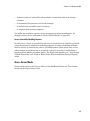
Model Basic Queueing Systems . . . . . . . . . . . . . . . . . . . . . . . .
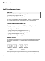
Constructs Involving Queues and Servers . . . . . . . . . . . . . . .
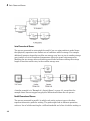
Example of a Logical Queue . . . . . . . . . . . . . . . . . . . . . . . . .
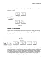
Vary the Service Time of a Server . . . . . . . . . . . . . . . . . . . .
4-6
4-6
4-9
4-10
Designing Paths for Entities
Role of Paths in SimEvents Models . . . . . . . . . . . . . . . . . . . . .
Definition of Entity Paths . . . . . . . . . . . . . . . . . . . . . . . . . . .
Implications of Entity Paths . . . . . . . . . . . . . . . . . . . . . . . . .
Overview of Routing Library for Designing Paths . . . . . . . . .
5-2
5-2
5-2
5-3
Select Departure Path Using Output Switch . . . . . . . . . . . . .
Role of the Output Switch . . . . . . . . . . . . . . . . . . . . . . . . . . .
Sample Use Cases . . . . . . . . . . . . . . . . . . . . . . . . . . . . . . . . .
Select the First Available Server . . . . . . . . . . . . . . . . . . . . . .
Use an Attribute to Select an Output Port . . . . . . . . . . . . . .
5-5
5-5
5-5
5-6
5-8
vii
6
viii
Contents
Select Arrival Path Using Input Switch . . . . . . . . . . . . . . . . .
Role of the Input Switch . . . . . . . . . . . . . . . . . . . . . . . . . . . .
Round-Robin Approach to Choosing Inputs . . . . . . . . . . . . . .
5-9
5-9
5-9
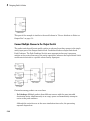
Combine Entity Paths . . . . . . . . . . . . . . . . . . . . . . . . . . . . . . .
Role of the Path Combiner . . . . . . . . . . . . . . . . . . . . . . . . .
Sequence Simultaneous Pending Arrivals . . . . . . . . . . . . . .
Path Combiner Versus Input Switch . . . . . . . . . . . . . . . . . .
5-12
5-12
5-13
5-15
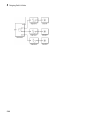
Model a Packet Switch . . . . . . . . . . . . . . . . . . . . . . . . . . . . . .
Overview . . . . . . . . . . . . . . . . . . . . . . . . . . . . . . . . . . . . . . .
Generate Packets . . . . . . . . . . . . . . . . . . . . . . . . . . . . . . . .
Store Packets in Input Buffers . . . . . . . . . . . . . . . . . . . . . .
Rout Packets to Their Destinations . . . . . . . . . . . . . . . . . . .
Connect Multiple Queues to the Output Switch . . . . . . . . . .
Model the Channels . . . . . . . . . . . . . . . . . . . . . . . . . . . . . .
5-16
5-16
5-17
5-18
5-19
5-20
5-21
Selected Bibliography
1
Introduction
• “SimEvents Product Description” on page 1-2
• “Discrete-Event Simulation in Simulink Models” on page 1-3
• “Related Products” on page 1-5
• “What Is an Entity?” on page 1-6
• “What Is an Event?” on page 1-7
• “Run a Sample Model” on page 1-9
1
Introduction
SimEvents Product Description
Model and simulate discrete-event systems
SimEvents provides a discrete-event simulation engine and component library for
Simulink®. You can model event-driven communication between components to analyze
and optimize end-to-end latencies, throughput, packet loss, and other performance
characteristics. Libraries of predefined blocks, such as queues, servers, and switches,
enable you to accurately represent your system and customize routing, processing delays,
prioritization, and other operations.
With SimEvents you can design distributed control systems, hardware architectures,
and sensor and communication networks for aerospace, automotive, and electronics
applications. You can also simulate event-driven processes, such as the execution
of a mission plan or the stages of a manufacturing process, to determine resource
requirements and identify bottlenecks.
Key Features
• Discrete-event simulation engine for multidomain modeling of complex systems in
Simulink
• Predefined block libraries, including queues, servers, generators, routing, and entity
combiner/splitter blocks
• Entities with custom data attributes for flexible representation of packets, tasks, and
parts
• Built-in statistics aggregation for obtaining delay, throughput, average queue length,
and other metrics
• Library blocks for defining domain-specific constructs, such as communication
channels, messaging protocols, and conveyor belts
• In-model animation for visualizing model operation and debugging
1-2
Discrete-Event Simulation in Simulink Models
Discrete-Event Simulation in Simulink Models
SimEvents software incorporates discrete-event system modeling into the Simulink timebased framework, which is suited for modeling continuous-time and periodic discretetime systems. In time-based systems, state updates occur synchronously with time. By
contrast, in discrete-event systems, state transitions depend on asynchronous discrete
incidents called events. Some examples illustrate these differences:
• Suppose you are interested in how long the average airplane waits in a queue for its
turn to use an airport runway. However, you are not interested in the details of how
an airplane moves once it takes off. You can use discrete-event simulation in which
the relevant events include:
• The approach of a new airplane to the runway
• The clearance for takeoff of an airplane in the queue.
• Suppose you are interested in the trajectory of an airplane as it takes off. You would
probably use time-based simulation because finding the trajectory involves solving
differential equations.
• Suppose you are interested in how long the airplanes wait in the queue. Suppose you
also want to model the takeoff in some detail instead of using a statistical distribution
for the duration of runway usage. You can use a combination of time-based simulation
and discrete-event simulation, where:
• The time-based aspect controls details of the takeoff
• The discrete-event aspect controls the queuing behavior
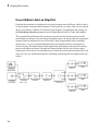
In a Simulink model, you typically construct a discrete-event system by adding a variety
of blocks, such as generators, queues, and servers, from the SimEvents block library.
These blocks are suitable for producing and processing entities, which are abstractions
of discrete items of interest. Examples of entities are packets within a communication
network, planes on a runway, or trains within a signaling system. Asynchronous events
that correspond to motion and changes in entity attributes through the system model
update the states of the underlying system. Examples of states are lengths of queues or
service time for an entity in a server.
One or more discrete-event systems can coexist with time-based systems in a Simulink
model. This coexistence facilitates the simulation of sophisticated hybrid systems. Using
special gateway blocks, you can pass signals from time-based components/systems to and
from discrete-event components/systems modeled with SimEvents blocks. These gateway
blocks enable time-based and event-based systems to share states. The combination
1-3
1
Introduction
of time- and event-based modeling facilitates the simulation of large-scale systems
that incorporate smaller subsystems from multiple environments. An example of a
large-scale system might have physical modeling for continuous-time systems, such as
electrical systems, which communicate via a channel modeled as a discrete-event system.
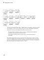
A Simulink model can also contain a purely discrete-event system with no time-based
components when modeling event-based processes. These systems are common in models
that represent logistic and manufacturing systems.
1-4
Related Products
Related Products
In this section...
“Information About Related Products” on page 1-5
“Limitations on Usage with Related Products” on page 1-5
Information About Related Products
For information about related products, see http://www.mathworks.com/products/
simevents/related.html.
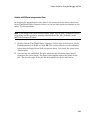
Limitations on Usage with Related Products
Code Generation
SimEvents blocks do not support code generation using the Simulink Coder™ product
in version 4.0 (R2011b). In previous versions up until version 3.1.2 (R2010a), SimEvents
blocks offered limited code generation support for rapid simulation. This support will
no longer be available for models upgraded to use the new SimEvents syntax in version
4.0 through the seupdate model update process. Support for rapid simulation has
been removed because the improvements in normal model simulation performance for
SimEvents models match or surpass the performance of rapid simulation in releases
prior to version 4.0.
Simulation Modes
SimEvents blocks do not support simulation using the Rapid Accelerator, Accelerator,
Processor-in-the-Loop (PIL), or External mode.
Model Reference
SimEvents blocks cannot be in a model that you reference through the Model block.
Function-Call Split Block
SimEvents blocks cannot connect to the Function-Call Split block. Instead, to split a
function-call signal that invokes or originates from a SimEvents block, use the SignalBased Event to Function-Call Event block as in “Issue Two Function Calls in Sequence”
in the SimEvents user guide documentation.
1-5
1
Introduction
What Is an Entity?
Discrete-event simulations typically involve discrete items of interest. By definition,
these items are called entities in SimEvents software. Entities can pass through a
network of queues, servers, gates, and switches during a simulation. Entities can carry
data, known in SimEvents software as attributes.
Note: Entities are not the same as events. Events are instantaneous discrete incidents
that change a state variable, an output, and/or the occurrence of other events. See “What
Is an Event?” on page 1-7 for details.
Examples of entities in some sample applications are in the table.
Context of Sample Application
Entities
Airport with a queue for runway access
Airplanes waiting for access to runway
Communication network
Packets, frames, or messages to transmit
Bank of elevators
People traveling in elevators
Conveyor belt for assembling parts
Parts to assemble
Computer operating system
Computational tasks or jobs
A graphical block can represent a component that processes entities, but entities
themselves do not have a graphical representation. When you design and analyze your
discrete-event simulation, you can choose to focus on:
• The entities themselves. For example, what is the average waiting time for a series of
entities entering a queue?
• The processes that entities undergo. For example, which step in a multiple-step
process (that entities undergo) is most susceptible to failure?
1-6
What Is an Event?
What Is an Event?
In this section...
“Overview of Events” on page 1-7
“Relationships Among Events” on page 1-7
“Viewing Events” on page 1-8
Overview of Events
In a discrete-event simulation, an event is an instantaneous discrete incident that
changes a state variable, an output, and/or the occurrence of other events. Examples of
events that can occur during simulation of a SimEvents model are:
• The advancement of an entity from one block to another.
• The completion of service on an entity in a server.
• A zero crossing of a signal connected to a block that you configure to react to zero
crossings. These events are also called trigger edges.
• A function call, which is a discrete invocation request carried from block to block by a
special signal called a function-call signal.
For a full list of supported events and more details on them, see “Events in SimEvents
Models”.
Relationships Among Events
Events in a simulation can depend on each other:
• One event can be the sole cause of another event. For example, the arrival of the first
entity in a queue causes the queue length to change from 0 to 1.
• One event can enable another event to occur, but only under certain conditions. For
example, the completion of service on an entity makes the entity ready to depart
from the server. However, the departure occurs only if the subsequent block is able to
accept the arrival of that entity. In this case, one event makes another event possible,
but does not solely cause it.
Events that occur at the same value of the simulation clock are called simultaneous
events, even if the application processes sequentially. When simultaneous events are
1-7
1
Introduction
not causally related to each other, the processing sequence can significantly affect the
simulation behavior. For an example, see “Choose Values for Event Priorities”. For more
details, see “Processing Sequence for Simultaneous Events” online.
Viewing Events
Events do not have a graphical representation. You can infer their occurrence by
observing their consequences, by using the Instantaneous Event Counting Scope block,
or by using the debugger. For details, see “Observe Events”, “Simulation Log in the
Debugger”, or “View the Event Calendar” online.
1-8
Run a Sample Model
Run a Sample Model
In this section...
“Overview of the Model” on page 1-9
“Accessing the Model” on page 1-9
“Examining Entities and Signals in the Model” on page 1-10
“Key Components of the Model” on page 1-12
“Running the Simulation” on page 1-13
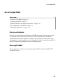
Overview of the Model
One way to become familiar with the basics of SimEvents models and the way they work
is to examine and run a previously built model. This section describes a SimEvents
example model. The model simulates a technique for dynamically adjusting the energy
consumption of a microcontroller based on the workload, without compromising quality of
service. Changes in the workload can occur as discrete events.
Accessing the Model
To read about this example, enter showdemo('sedemo_DVS_model') in the MATLAB®
Command Window.
1-9
1
Introduction
Click Open This Example to open the model.
Examining Entities and Signals in the Model
This section describes the different kinds of ports and lines that appear in the
sedemo_DVS_model model. Compared to signal ports, entity ports look different and
represent a different concept.
Entity Ports and Connections
Some blocks in this model can process entities, which the “What Is an Entity?” on page
1-6 section discusses.
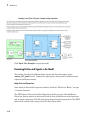
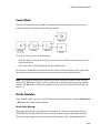
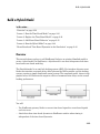
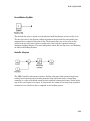
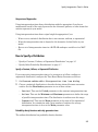
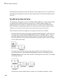
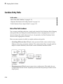
The FIFO Queue block and the Start Timer block, which are part of the SimEvents
library set, process entities in this model. Each of these blocks has an entity input port
and an entity output port. The following figure shows the entity output port of the FIFO
Queue block and the entity input port of the Start Timer block.
1-10
Run a Sample Model
Entity connection line
Entity
output
port
Entity
input
port
Entity connection lines represent relationships among two blocks (or among their entity
ports) by indicating a path by which an entity can:
• Depart from one block
• Arrive simultaneously at a subsequent block
The preceding figure shows the connection line:
• From OUT, the entity output port of the FIFO Queue block
• To IN, the entity input port of the Start Timer block
When you run the simulation, entities that depart from the OUT port arrive
simultaneously at the IN port.
By convention, entity ports use labels with words in uppercase letters, such as IN and
OUT.
You cannot branch an entity connection line. If your application requires an entity to
arrive at multiple blocks, use the Replicate block to create copies of the entity.
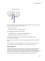
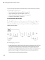
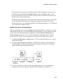
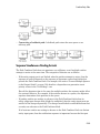
Signals and Signal Ports
Some blocks in this model can process signals. Signals represent numerical quantities
defined at all times during a simulation, not only at a discrete set of times. Signals
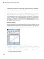
appear as connection lines between signal ports of two blocks. The following figure shows
that the Start Timer block has not only an entity output port but also a signal output
port. The signal output port connects to the Random Service Time subsystem.
1-11
1
Introduction
Signal
connection
line
Signal input port
Signal
output
port
In a discrete-event system, the signal input port coming into a block changes to an empty
arrow when you perform update diagram:
Key Components of the Model
The sedemo_DVS_model model uses event-based blocks to simulate the workload of the
microcontroller:
• At random times, the Time-Based Entity Generator block generates an entity that
represents a job for the microcontroller.
• The FIFO Queue block stores jobs that the microcontroller cannot process
immediately.
• The Single Server block models the processing of a job by the microcontroller.
1-12
Run a Sample Model
This block can process at most one job at a time and thus limits the availability of the
microcontroller to process new jobs. While a job is in this block, other jobs remain in
the FIFO Queue block.
• The Start Timer and Read Timer blocks work together to compute the time that each
job spends in the server. The result of the computation is the et output signal from
the Read Timer block.
• The Entity Sink block absorbs jobs that have completed their processing.
• Between the blocks where event-based signals transition to signal-based signals,
Event to Timed Signal block performs the conversion.
Important discrete events in this model are the generation of a new job and the
completion of processing of a job.
The model also includes blocks that simulate a dynamic voltage scaling (DVS) controller
that adjusts the input voltage depending on the workload of the microcontroller. The
idea is to minimize the average cost per job, where the cost takes into account both
energy consumption and quality of service. For more information about the cost and
the optimization technique, see Modeling Load Within a Dynamic Voltage Scaling
Application online.
Appearance of Entities
Entities do not appear explicitly in the model window. However, you can gather
information about entities using plots, signals, and entity-related features in the
debugger. See these sections for more information:
• “Synchronize Service Start Times with the Clock” online
• “Select the First Available Server” on page 5-6
• “Plot the Queue-Length Signal” on page 2-20, which is part of the larger example
“Build a Discrete-Event Model” on page 2-2
• “Inspect Entities” online
Running the Simulation
To run the sedemo_DVS_model simulation, choose Simulation > Run from the model
window. A Figure window opens with a dynamic plot showing how the DVS controller
varies the voltage during the simulation to reduce the average cost per job. A triangle
marker moves to indicate the current voltage and corresponding cost.
1-13
1
Introduction
1-14
2
Building Simple Models with
SimEvents Software
• “Build a Discrete-Event Model” on page 2-2
• “Explore Simulations Using the Debugger and Plots” on page 2-17
• “Build a Hybrid Model” on page 2-29
• “Key Concepts in SimEvents Software” on page 2-43
2
Building Simple Models with SimEvents Software
Build a Discrete-Event Model
In this section...
“Overview” on page 2-2
“Open a Model and Libraries” on page 2-3
“Move Blocks into the Model Window” on page 2-5
“Configure Blocks” on page 2-10
“Connect Blocks” on page 2-13
“Run the Simulation” on page 2-13
“Insert Blocks” on page 2-15
“Build a Model Using Model Construction Commands” on page 2-15
Overview
This section describes how to build a new model representing a discrete-event system.
The system is a simple queuing system in which “customers” — entities — arrive at a
fixed deterministic rate, wait in a queue, and advance to a server that operates at a fixed
deterministic rate. This type of system is known as a D/D/1 queuing system in queuing
notation. The notation indicates a deterministic arrival rate, a deterministic service rate,
and a single server.
Using the example system, this section shows you how to perform basic model-building
tasks, such as:
• Adding blocks to models
• Configuring blocks using their parameter dialog boxes
The next section, “Explore Simulations Using the Debugger and Plots” on page 2-17,
uses the same D/D/1 system to illustrate techniques more specific to discrete-event
simulations, such as:
• Using the SimEvents debugger to examine the state of a server
• Using plots to understand simulation behavior, including plots that show multiple
values at a fixed time
To skip the model-building steps and open a completed version of the example model,
enter simeventsdocex('doc_dd1') in the MATLAB Command Window. Save the model in
your working folder as dd1.
2-2
Build a Discrete-Event Model
Note: When you later create your own models, use the conversion blocks from the
Gateways library (gateway blocks) to convert signals and function-calls from signal-based
to event-based and vice versa.
Open a Model and Libraries
The first steps in building a model are to set up your environment, open a new model
window, and open the libraries containing blocks.
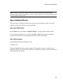
Open a New Model Window
On the Home tab, select New > Simulink Model . An empty model window opens.
To name the model and save it as a file, select File > Save from the model window's
menu. Save the model in your working folder under the file name dd1.
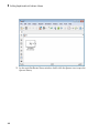
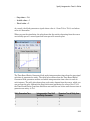
Open SimEvents Libraries
In the MATLAB Command Window, enter
simeventslib
The main SimEvents library window appears. This window contains an icon for each
SimEvents library. To open a library and view the blocks it contains, double-click the icon
that represents that library.
2-3
2
Building Simple Models with SimEvents Software
Open Simulink Libraries
In the MATLAB Command Window, enter
simulink
The Simulink Library Browser opens, using a tree structure to display the available
libraries and blocks. To view the blocks in a library listed in the left pane, select the
library name, and the list of blocks appears in the right pane. The Library Browser
provides access not only to Simulink blocks but also to SimEvents blocks. For details
about the Library Browser, see “Block Library Basics”.
2-4
Build a Discrete-Event Model
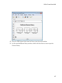
Move Blocks into the Model Window
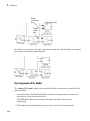
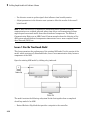
To move blocks from libraries into the model window, follow these steps:
1
In the main SimEvents library window, double-click the Generators icon to open the
Generators library. Then double-click the Entity Generators icon to open the Entity
Generators sublibrary.
2
Drag the Time-Based Entity Generator block from the library into the model
window.
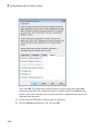
This might cause an informational dialog box to open, with a brief description of the
difference between entities and events.
2-5
2
Building Simple Models with SimEvents Software
3
2-6
In the main SimEvents library window, double-click the Queues icon to open the
Queues library.
Build a Discrete-Event Model
4
Drag the FIFO Queue block from the library into the model window.
5
In the main SimEvents library window, double-click the Servers icon to open the
Servers library.
2-7
2
2-8
Building Simple Models with SimEvents Software
6
Drag the Single Server block from the library into the model window.
7
In the main SimEvents library window, double-click the SimEvents Sinks icon to
open the SimEvents Sinks library.
Build a Discrete-Event Model
8
Drag the Signal Scope block and the Entity Sink block from the library into the
model window.
As a result, the model window looks like the following figure. The model window contains
blocks that represent the key processes in the simulation: blocks that generate entities,
store entities in a queue, serve entities, and create a plot showing relevant data.
2-9
2
Building Simple Models with SimEvents Software
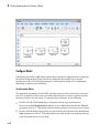
Configure Blocks
Configuring the blocks in dd1 means setting their parameters appropriately to represent
the system being modeled. Each block has a dialog box that enables you to specify
parameters for the block. Default parameter values might or might not be appropriate,
depending on what you are modeling.
View Parameter Values
Two important parameters in this D/D/1 queuing system are the arrival rate and service
rate. The reciprocals of these rates are the duration between successive entities and the
duration of service for each entity. To examine these durations, do the following:
2-10
1
Double-click the Time-Based Entity Generator block to open its dialog box.
Observe that the Distribution parameter is set to Constant and that the Period
parameter is set to 1. This means that the block generates a new entity every second.
2
Double-click the Single Server block to open its dialog box. Observe that the Service
time parameter is set to 1. This means that the server spends one second processing
each entity that arrives at the block.
Build a Discrete-Event Model
3
Click Cancel in both dialog boxes to dismiss them without changing any
parameters.
The Period and Service time parameters have the same value, which means that the
server completes an entity's service at exactly the same time that a new entity is being
created.
Change Parameter Values
Configure blocks to create a plot that shows when each entity departs from the server,
and to make the queue have an infinite capacity. Do this as follows:
1
Double-click the Single Server block to open its dialog box.
2
Click the Statistics tab to view parameters related to the statistical reporting of the
block.
3
Select the Number of entities departed check box.
2-11
2
Building Simple Models with SimEvents Software
Then click OK. The Single Server block acquires a signal output port labeled #d.
During the simulation, the block will produce an output signal at this #d port; the
signal's value is the running count of entities that have completed their service and
departed from the server.
2-12
4
Double-click the FIFO Queue block to open its dialog box.
5
Set the Capacity parameter to Inf and click OK.
Build a Discrete-Event Model
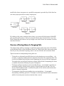
Connect Blocks
Now that the model window for dd1 contains blocks that represent the key processes,
connect the blocks as shown in the following graphic.
To connect blocks, do one of the following:
• With the mouse, drag from the output port of the source block to the input port of the
destination block.
• Select the source block. Ctrl+click the destination block.
In both cases, SimEvents connects the source block to the destination block. If necessary,
the software also routes the connecting line around intervening blocks or lines.
Note: The following section about inserting blocks is general information that does not
apply to the dd1 model. When you have connected the blocks as shown in the preceding
graphic, the dd1 model is ready for simulation as described in “Run the Simulation” on
page 2-13.
Run the Simulation
Save the dd1 model you have created. Then start the simulation by choosing Simulation
> Run from the model window's menu.
Resolve Solver Warnings
When you first simulate the model in this example, you will see warning messages in
the MATLAB Command Window about continuous states and the maximum step size.
These messages appear because certain default parameters for a Simulink model are
2-13
2
Building Simple Models with SimEvents Software
inappropriate for this particular example model, which is completely event-based and
contains no blocks with continuous states. The application overrides the inappropriate
parameters and alerts you to that fact.
If you want to prevent these warnings when you simulate event-based models in the
future, you need to set the solver type and step size parameters to appropriate values.
To do this, with your model open in the model editor, open Simulation > Configuration
Parameters > Solver. Under the Solver options section, for the Type: parameter select
the Variable-step option in the drop-down list. For the Solver: parameter, select
Discrete in the drop-down list and in the field for the Max step size: parameter, type
inf. Click OK and save your model.
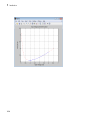
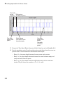
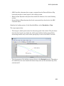
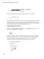
Results of the Simulation
When the simulation runs, the Signal Scope block opens a window containing a plot. The
horizontal axis represents the times at which entities depart from the server, while the
vertical axis represents the total number of entities that have departed from the server.
After an entity departs from the Single Server block, the block updates its output signal
at the #d port. The updated values are reflected in the plot and highlighted with plotting
markers. From the plot, you can make these observations:
• Until T=1, no entities depart from the server. This is because it takes one second for
the server to process the first entity.
2-14
Build a Discrete-Event Model
• Starting at T=1, the plot is a stairstep plot. The stairs have height 1 because the
server processes one entity at a time, so entities depart one at a time. The stairs have
width equal to the constant service time, which is one second.
Insert Blocks
You can insert a block in an existing line, if the block that you want to insert:
• Has only one input and one output port.
• Has connection port types (i.e. entity ports or signal ports) that correspond with the
data on the existing line. For example, in an existing entity line, you can insert only
a block that accepts and outputs entities. You cannot insert a block that accepts and
outputs event-based signals.
To insert a block in a line:
1
Drag the block over the line.
2
Release the mouse button. SimEvents inserts the block in the line.
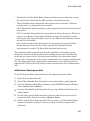
Build a Model Using Model Construction Commands
This example shows how to use model construction commands to add blocks to a model
and connect them.
Suppose you want to add a Time-Based Entity Generator block and a FIFO Queue block
to a model and connect them:
This procedure shows you how to add and position the two blocks in a model, for
example, MyModel.
Add the Time-Based Entity Generator block and position it.
add_block(['simeventslib/Generators/Entity Generators/', ...
'Time-Based Entity Generator'], 'MyModel/Time-Based Entity Generator');
2-15
2
Building Simple Models with SimEvents Software
set_param('MyModel/Time-Based Entity Generator','position',[65 63 150 117]);
The position parameter specifies the top left (x,y) and lower right (x+block width, y
+block height) corners of the block.
Add the FIFO Queue block and position it.
add_block('simeventslib/Queues/FIFO Queue','MyModel/FIFO Queue');
set_param('MyModel/FIFO Queue','position',[195 63 280 117]);
Connect the blocks.
add_line('MyModel','Time-Based Entity Generator/RConn1','FIFO Queue/LConn1','autorouting','on');
Port indices, such as Time-Based Entity Generator/RConn1, correspond to the topdown order of connection ports when you look at the block in the Simulink Editor. The
autorouting feature routes lines around any intervening blocks or other lines, as needed.
Note: If you want to connect blocks that are inside a subsystem, use the full path to the
subsystem as the first argument of the add_line function:
add_line('MyModel/MySubsystem', 'Time-Based Entity Generator/RConn1',... )
2-16
Explore Simulations Using the Debugger and Plots
Explore Simulations Using the Debugger and Plots
In this section...
“Explore the D/D/1 System Using the SimEvents Debugger” on page 2-17
“Explore the D/D/1 System Using Plots” on page 2-19
“Information About Race Conditions and Random Times” on page 2-28
Explore the D/D/1 System Using the SimEvents Debugger
The plot in “Run the Simulation” on page 2-13 indicates how many entities have
departed from the server, but does not address the following question: Is any entity still
in the server at the conclusion of the simulation? To answer the question, you can use the
SimEvents debugger, as described in this section. Using the debugger involves running
the simulation in a special debugging mode that lets you suspend a simulation at each
step or breakpoint and query simulation behavior. Using the debugger does not require
you to change the model. The topics in this section are as follows:
• “Start the Debugger” on page 2-17
• “Run the Simulation” on page 2-18
• “Query the Server Block” on page 2-18
• “End the Simulation” on page 2-19
• “For Further Information” on page 2-19
Start the Debugger
To open a completed version of the example model for this tutorial, enter
simeventsdocex('doc_dd1') in the MATLAB Command Window. Save the model in your
working folder as dd1.
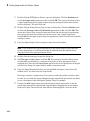
To start simulating the current system in debugging mode, enter this command at the
MATLAB command prompt:
sedebug(bdroot)
The output in the MATLAB Command Window indicates that the debugger is active. The
output also includes hyperlinks to information sources.
*** SimEvents Debugger ***
2-17
2
Building Simple Models with SimEvents Software
Functions | Help | Watch Video Tutorial
%==============================================================================%
Initializing Model dd1
sedebug>>
The sedebug>> notation is the debugger prompt, where you enter commands.
Run the Simulation
The simulation has initialized but does not proceed. In debugging mode, you indicate
to the debugger when to proceed through the simulation and how far to proceed before
returning control to you. The purpose of this example is to find out whether an entity is
in the server when the simulation ends. To continue the simulation until it ends, enter
this command at the sedebug>> prompt:
cont
The Command Window displays a long series of messages that indicate what is
happening during the simulation. The end of the output indicates that the debugger has
suspended the simulation just before the end:
Hit built-in breakpoint for the end of simulation.
Use 'cont' to end the simulation or any other function to inspect final states of the
system.
%==============================================================================%
Terminating Model dd1
To understand the long series of messages, see “Simulation Log in the Debugger”.
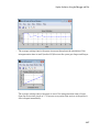
Query the Server Block
The debugger has suspended the simulation just before the end and the sedebug>>
prompt indicates that you can still enter debugging commands. In this way, you have an
opportunity to inspect the final states of blocks or other aspects of the simulation. To get
information about the Single Server block, enter this command:
blkinfo('dd1/Single Server')
The output shows the state of the Single Server block at the current time, T=10. The last
two rows of the output represent a table that lists entities in the block. The table has one
row because the server is currently storing one entity. The entity has a unique identifier,
en11, and is currently in service. This output affirmatively answers the question of
whether an entity is in the server when the simulation ends.
2-18
Explore Simulations Using the Debugger and Plots
One entity
is in service
Table of entities in the block
End the Simulation
The simulation is still suspended just before the end. To proceed, enter this command:
cont
The simulation ends, the debugging session ends, and the MATLAB command prompt
returns.
For Further Information
For additional information about the SimEvents debugger, see “Debug Simulation”.
Explore the D/D/1 System Using Plots
The dd1 model that you created in “Build a Discrete-Event Model” on page 2-2 plots the
number of entities that depart from the server. This section modifies the model to plot
other quantities that can reveal aspects of the simulation. The topics are as follows:
• “Enable the Queue-Length Signal” on page 2-20
• “Plot the Queue-Length Signal” on page 2-20
• “Simulate with Different Intergeneration Times” on page 2-21
• “View Waiting Times and Utilization” on page 2-23
• “Observations from Plots” on page 2-25
To open a completed version of the example model for this tutorial, enter
simeventsdocex('doc_dd1') in the MATLAB Command Window. Before modifying the
model, save it with a different file name.
2-19
2
Building Simple Models with SimEvents Software
Enable the Queue-Length Signal
The FIFO Queue block can report the queue length, that is, the number of entities it
stores at a given time during the simulation. To configure the FIFO Queue block to
report its queue length, do the following:
1
Double-click the FIFO Queue block to open its dialog box. Click the Statistics tab to
view parameters related to the statistical reporting of the block.
2
Set the Number of entities in queue parameter to On and click OK. This causes
the block to have a signal output port for the queue-length signal. The port label is
#n.
Plot the Queue-Length Signal
The model already contains a Signal Scope block for plotting the entity count signal.
To add another Signal Scope block for plotting the queue-length signal (enabled above),
follow these steps:
2-20
1
In the main SimEvents library window, double-click the SimEvents Sinks icon to
open the SimEvents Sinks library.
2
Drag the Signal Scope block from the library into the model window. The block
automatically assumes a unique block name, Signal Scope1, to avoid a conflict with
the existing Signal Scope block in the model.
3
Connect the #n signal output port of the FIFO Queue block to the in signal input
port of the Signal Scope1 block by dragging the mouse pointer from one port to the
other. The model now looks like the following figure.
Explore Simulations Using the Debugger and Plots
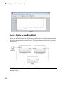
Simulate with Different Intergeneration Times
By changing the intergeneration time (that is, the reciprocal of the entity arrival rate)
in the Time-Based Entity Generator block, you can see when entities accumulate in the
queue. Try this procedure:
Note: If you skipped the earlier model-building steps, you can open a completed version
of the model for this section by entering simeventsdocex('doc_dd1_blockage') in the
MATLAB Command Window.
1
Double-click the Time-Based Entity Generator block to open its dialog box, set the
Period parameter to 0.85, and click OK. This causes entities to arrive somewhat
faster than the Single Server block can process them. As a result, the queue is not
always empty.
2
Save and run the simulation. The plot whose title bar is labeled Signal Scope1
represents the queue length. The figure below explains some of the points on the
plot. The vertical range on the plot has been modified to fit the data better.
2-21
2
Building Simple Models with SimEvents Software
First entity
Entity arrives
arrives
at queue and stays in queue
First entity
departs from
queue
Entity departs
from queue, which
becomes empty
One entity
departs from
queue.
One entity
remains in
queue.
3
Reopen the Time-Based Entity Generator block's dialog box and set Period to 0.3.
4
Run the simulation again. Now the entities arrive much faster than the server can
process them. You can make these observations from the plot:
• Every 0.3 s, the queue length increases because a new entity arrives.
• Every 1 s, the queue length decreases because the server becomes empty and
accepts an entity from the queue.
• Every 3 s, the queue length increases and then decreases in the same time
instant. The plot shows two markers at T = 0, 3, 6, and 9.
2-22
Explore Simulations Using the Debugger and Plots
5
Reopen the Time-Based Entity Generator block's dialog box and set Period to 1.1.
6
Run the simulation again. Now the entities arrive more slowly than the server's
service rate, so every entity that arrives at the queue is able to depart in the same
time instant. The queue length is never greater than zero for a positive amount of
time.
View Waiting Times and Utilization
The queue length is an example of a statistic that quantifies a state at a particular
instant. Other statistics, such as average waiting time and server utilization, summarize
behavior between T=0 and the current time. To modify the model so that you can view
the average waiting time of entities in the queue and server, as well as the proportion of
time that the server spends storing an entity, use the following procedure:
Note: To skip the model-building steps and open a completed version of the model for this
section, enter simeventsdocex('doc_dd1_wait_util') in the MATLAB Command Window.
Then skip to step 8 to run the simulation.
2-23
2
Building Simple Models with SimEvents Software
1
Double-click the FIFO Queue block to open its dialog box. Click the Statistics tab,
set the Average wait parameter to On, and click OK. This causes the block to have
a signal output port for the signal representing the average duration that entities
wait in the queue. The port label is w.
2
Double-click the Single Server block to open its dialog box. Click the Statistics tab,
set both the Average wait and Utilization parameters to On, and click OK. This
causes the block to have a signal output port labeled w for the signal representing
the average duration that entities wait in the server, and a signal output port
labeled util for the signal representing the proportion of time that the server spends
storing an entity.
3
Copy the Signal Scope1 block and paste it into the model window.
Note: If you modified the plot corresponding to the Signal Scope1 block, then one
or more parameters in its dialog box might be different from the default values.
Copying a block also copies parameter values.
4
Double-click the new copy to open its dialog box.
5
Set Plot type to Continuous and click OK. For summary statistics like average
waiting time and utilization, a continuous-style plot is more appropriate than a
stairstep plot. Note that the Continuous option refers to the appearance of the plot
and does not change the signal itself to make it continuous-time.
6
Copy the Signal Scope2 block that you just modified and paste it into the model
window twice. You now have five scope blocks.
Each copy assumes a unique name. If you want to make the model and plots easier
to read, you can click the names underneath each scope block and rename the block
to use a descriptive name like Queue Waiting Time, for example.
7
2-24
Connect the util signal output port and the two w signal output ports to the in
signal input ports of the unconnected scope blocks by dragging the mouse pointer
from port to port. The model now looks like the following figure. Save the model.
Explore Simulations Using the Debugger and Plots
8
Run the simulation with different values of the Period parameter in the
Time-Based Entity Generator block, as described in “Simulate with Different
Intergeneration Times” on page 2-21. Look at the plots to see how they change if
you set the intergeneration time to 0.3 or 1.1, for example.
Observations from Plots
• The average waiting time in the server does not change after the first departure from
the server because the service time is fixed for all departed entities. The average
waiting time statistic does not include partial waiting times for entities that are in
the server but have not yet departed.
2-25
2
Building Simple Models with SimEvents Software
• The utilization of the server is nondecreasing if the intergeneration time is small
(such as 0.3) because the server is constantly busy once it receives the first entity.
The utilization might decrease if the intergeneration time is larger than the service
time (such as 1.5) because the server has idle periods between entities.
2-26
Explore Simulations Using the Debugger and Plots
• The average waiting time in the queue increases throughout the simulation if the
intergeneration time is small (such as 0.3) because the queue gets longer and longer.
The average waiting time in the queue is zero if the intergeneration time is larger
than the service time (such as 1.1) because every entity that arrives at the queue is
able to depart immediately.
2-27
2
Building Simple Models with SimEvents Software
Information About Race Conditions and Random Times
Other examples modify this one by varying the processing sequence for simultaneous
events or by making the intergeneration times and/or service times random. The
modified examples are:
• “Using Random Intergeneration Times in a Queuing System” on page 3-8
• “Random Service Times in a Queuing System” on page 4-11
2-28
Build a Hybrid Model
Build a Hybrid Model
In this section...
“Overview” on page 2-29
“Lesson 1: Run the Time-Based Model” on page 2-30
“Lesson 2: Explore the Time-Based Model” on page 2-32
“Lesson 3: Add Event-Based Behavior” on page 2-35
“Lesson 4: Run the Hybrid Model” on page 2-40
“Event-Based and Time-Based Dynamics in the Simulation” on page 2-42
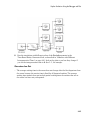
Overview
This tutorial shows you how to add SimEvents blocks to an existing Simulink model to
create a hybrid model. In SimEvents, a hybrid model is one that incorporates both timebased and event-based modeling.
The Simulink model is an anti-lock braking system (ABS). You introduce discrete-event
blocks that simulate a network delay effect between the ABS controller and the braking
system, creating a simple distributed control system. The completed model, shown in the
graphic below, will illustrate the negative effects of communication delays on the overall
braking performance.
You will:
• Use SimEvents gateway blocks to convert time-based signals to event-based signals
and vice-versa.
• Attach data from time-based dynamics to SimEvents entities whose timing is
independent of the time-based dynamics.
2-29
2
Building Simple Models with SimEvents Software
• Use discrete events to update signals that influence time-based dynamics.
• Adjust parameters in the discrete-event system to affect the results of the overall
hybrid model.
Note: A more realistic way to represent a distributed control system is to model
communication over a shared network, where time delays and transmission failures
might depend on network traffic from other distributed components. The Effects of
Communication Delays on an ABS Control System example shows the behavior of the
ABS system when distributed components communicate over a more complex Control
Area Network (CAN) bus.
Lesson 1: Run the Time-Based Model
This lesson examines the performance of the existing ABS model. In this version of the
model, which contains only Simulink blocks, there is no communication delay between
components of the ABS.
Open the existing ABS model by clicking abs_timebased.
The model contains the following subsystem blocks that together form a completed
closed-loop model of an ABS:
• Desired Relative Slip block that provides a setpoint to the controller.
2-30
Build a Hybrid Model
• ABS Controller subsystem that accepts a setpoint from the Desired Relative Slip
block and provides a control signal to the braking system.
• Brake System Dynamics subsystem that models the behavior of an actual braking
system.
• Sensor Relative Slip subsystem that feeds a measured slip value back to the ABS
Controller block.
Simulate the braking system. In the Simulink Editor, select Simulation > Run.
The scope outputs show:
• The change in wheel speed versus the decreasing speed of the vehicle. The plot shows
that the wheel speed stays below the vehicle speed without locking up (suddenly
decreasing towards zero), with vehicle speed going to zero in less than 15 seconds.
• The slip response of the braking system relative to the Desired setpoint. Throughout
the simulation, the error between the desired slip value and the measured slip value
remains small.
2-31
2
Building Simple Models with SimEvents Software
Lesson 2: Explore the Time-Based Model
Before you modify the model to add discrete-event behavior, you should understand how
the time-based portion of the model works. This lesson examines each block in the timebased model.
Note: For a more detailed analysis of a similar ABS model, see Modeling an Anti-Lock
Braking System.
2-32
Build a Hybrid Model
Desired Relative Slip Block
The desired slip value is based on some physical modeling known as the mu-slip curve.
The mu-slip curve is the friction coefficient between the tire and the road surface, mu,
expressed as an empirical function of slip. The desired slip is set to the value of slip
at which the mu-slip curve reaches a peak value, this being the optimum value for
minimum braking distance. For more information about the mu-slip curve, see Modeling
an Anti-Lock Braking System.
Controller Subsystem
The ABS Controller subsystem contains a further subsystem that executes bang-bang
control, based upon the error between measured slip and desired slip. A bang-bang
controller is a type of feedback controller that switches between two states, based on the
sign of the error signal at its input. In this model, the output of the bang-bang controller
translates to an on/off rate that is supplied to the braking system.
2-33
2
Building Simple Models with SimEvents Software
Brake System Dynamics Subsystem
The Brake System Dynamics subsystem is complex. What follows is a high-level
examination of how it works. For a more detailed analysis of a similar system, see
Modeling an Anti-Lock Braking System.
The Brake System Dynamics subsystem:
• Accepts a control signal from the ABS Controller subsystem, based on the error
between measured slip and desired slip.
• Delays the signal from the ABS Controller subsystem to model the delay associated
with the hydraulic lines of an actual braking system.
• Integrates the on/off rate supplied by the ABS Controller subsystem, to determine the
required braking pressure.
• Multiplies the brake pressure signal by the area and radius of the hydraulic braking
system piston, relative to the wheel, to determine the brake torque that is applied to
the wheel.
• Uses the calculated brake torque to calculate the wheel speed.
• Uses both the vehicle weight and the friction coefficient between the tire and the road
surface to determine the vehicle speed.
• Calculates the relative slip, based on the wheel speed, the vehicle speed, and the
minimum required stopping distance.
2-34
Build a Hybrid Model
Sensor Relative Slip Subsystem
The Sensor Relative Slip subsystem contains a Gain block where you can specify the
accuracy of the sensor in converting the actual relative slip to a measured value that
feeds back to the controller. A gain value of 1 simulates the ideal case of a sensor that
measures the slip with 100% accuracy.
Lesson 3: Add Event-Based Behavior
In this lesson, you’ll create the hybrid model by adding blocks from the SimEvents
library to the model introduced in “Lesson 1: Run the Time-Based Model” on page
2-30. To simplify the top-level view of the model, the SimEvents blocks are placed in
a subsystem. This subsystem models a communication delay between the ABS controller
and the braking system. The communication delay is a simple representation of the
delay effect that distributed components might experience when they communicate over
a heavily-loaded in-vehicle network. Each SimEvents entity in the delay subsystem
represents a data packet that conveys control signal information between the controller
and the braking system.
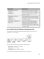
Top-Level View of Completed Hybrid Model
The completed model will look as shown in the preceding graphic. Both the ABS
Controller and Brake System Dynamics blocks are time-based systems. The Network
Delay subsystem block is an event-based system. In SimEvents, when signals transition
between the time-based domain and the event-based domain, or vice-versa, the blocks in
the Gateways block library manage this signal conversion.
2-35
2
Building Simple Models with SimEvents Software
To learn about the Network Delay subsystem behavior and for instructions on building
and integrating the subsystem, see:
• “How the Network Delay Subsystem Works” on page 2-36
• “Add the Network Delay Subsystem Block” on page 2-37
• “Add the Network Delay Subsystem Contents” on page 2-38
• “Complete the Hybrid Model” on page 2-39
How the Network Delay Subsystem Works
The Network Delay subsystem models a communication link that samples information
from the ABS controller and conveys that information to the braking system. The
following sections discuss how the network delay subsystem works, before providing
instructions to build the subsystem and integrate it with the existing ABS system to
complete the hybrid model.
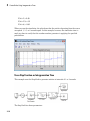
Network Delay Subsystem Contents
• A control signal from the ABS Controller block enters the subsystem via the In1 block.
The Timed to Event Signal gateway block converts the time-based signal from the
controller into an event-based signal, so that the data is available to the discreteevent blocks. In any SimEvents model, the way that the software converts time-based
signals to event-based signals depends on the solver you use for your simulation.
In this tutorial, the model uses a variable-step solver. For more information, see
“Variable-Step Solvers for Discrete-Event Systems”.
2-36
Build a Hybrid Model
• Periodically, the Time-Based Entity Generator block creates an entity that conveys
the control signal value from the ABS controller to the braking system.
• The Set Attribute block attaches the control signal value to the entity. This datacarrying entity is a data packet in the network.
• The N-Server block models the latency in the communication system by delaying each
data packet.
• The Get Attribute block models the reconstruction of data at the receiver. This block
connects to an Event to Timed Signal block that converts the data back to a timebased signal. This time-based signal connects to the Brake System Dynamics block at
the top level of the model.
• Once the time-based control signal departs the subsystem and enters the Brake
System Dynamics block, the entity that carries the data through the delay
susbsystem is not needed. The Entity Sink block absorbs the entity.
This subsystem models communication from the controller to the braking system,
but does not model the feedback path from the braking system to the controller. The
model that you create is only a first step toward modeling a true distributed control
system, where all components of the system communicate over a common communication
bus. Next steps might involve modeling the communication in the feedback path and
replacing the N-Server block with a more realistic representation of the communication
link.
Add the Network Delay Subsystem Block
To add the Network Delay subsystem block to the original time-based model:
1
Open the abs_timebased model.
2
Select File > Save As. Save the model to your working folder as abs_hybrid.
3
Open the Simulink and SimEvents libraries. In the MATLAB Command Window
enter simulink and simevents.
4
From the Simulink Ports & Subsystems library, drag a Subsystem block into the
model window.
5
For the newly inserted Subsystem block, place the cursor in the text box that is
beneath the block. Type the new name, Network Delay.
6
Double-click the Delay Subsystem block. The procedure, “Add the Network Delay
Subsystem Contents” on page 2-38 shows you how to build the contents of the
subsystem.
2-37
2
Building Simple Models with SimEvents Software
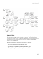
Add the Network Delay Subsystem Contents
In this procedure, you add event-based blocks that model a communications delay to the
Network Delay subsystem block. When you complete the procedure, the contents of the
Network Delay block should look as shown in the graphic.
2-38
1
In the SimEvents library, double-click the Generators library. Double-click the
Entity Generators sublibrary and drag a Time-Based Entity Generator block into
the subsystem window.
2
To review the entity generation behavior of the Time-Based Entity Generator block,
double-click it. The default value of Generate entities upon is Intergeneration
time from dialog, with a default intergeneration period of 1 s. Accept these
default values without making any change by clicking Cancel.
3
In the Generators library, double-click the he Signal Generators sublibrary.
Drag the Event-Based Random Number block into the subsystem window.
4
Double-click the Event-Based Random Number block. Set Distribution to Uniform,
Minimum to 0.01, and Maximum to 0.06. Click OK. These settings ensure that
the service time of the N-Server block varies with a uniform distribution of values
between a minimum of 0.01s and a maximum of 0.06s.
5
From the Attributes library, drag the Set Attribute and Get Attribute blocks into
the subsystem window.
6
Double-click the Set Attribute block. The Set Attribute tab of the dialog box
contains a table. On the first row of the table, set Name to Value and set Value
From to Signal port. Click OK. The block acquires an extra signal input port,
Value.
Build a Hybrid Model
7
Double-click the Get Attribute block. The Get Attribute tab of the dialog box
contains a table. On the first row of the table, set Name to Value. Click OK. The
block acquires an extra signal output port, Value.
8
From the Servers library, drag the N-Server block into the subsystem window.
9
Double-click the N-Server block. Set Service time from to Signal port t. Click
OK. The block acquires an extra signal input port, t.
10 From the SimEvents Sinks library, drag an Entity Sink block into the subsystem
window.
11 From the Gateways library, drag a Timed to Event Signal block and an Event to
Timed Signal block into the subsystem window.
12 Connect and place the blocks as shown in Network Delay Subsystem Contents.
13 Navigate to the top-level view of the model. Select View > Navigate > Up to
Parent. Save the model.
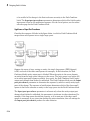
Complete the Hybrid Model
Before you connect the newly created Network Delay subsystem block to complete the
hybrid model, simplify the top-level view of the original ABS model by grouping related
blocks. When you complete this procedure, the model looks as shown in Top-Level View of
Completed Hybrid Model.
1
To select both the Desired Relative Slip and ABS Controller blocks of the model,
hold down the left mouse button and drag the mouse. As you drag the mouse, a box
appears. Drag this box across a portion of both blocks. When you release the mouse
button, the two blocks are highlighted in blue.
2
Right-click one of the two highlighted blocks and select Create Subsystem from
Selection. The software places both blocks inside a new Subsystem block.
3
For the newly created Subsystem block, place the cursor in the text box that is
beneath the block. type the new name, ABS Controller.
4
To select both the Brake System Dynamics and Sensor Relative Slip blocks of the
model, hold down the left mouse button and drag the mouse. As you drag the mouse,
a box appears. Drag this box across a portion of both blocks. When you release the
mouse button, the two blocks are highlighted in blue.
5
Right-click one of the two highlighted blocks and select Create Subsystem from
Selection. The software places both blocks inside a new Subsystem block.
6
For the newly created Subsystem block, place the cursor in the text box that is
beneath the block. type the new name, Brake System Dynamics.
2-39
2
Building Simple Models with SimEvents Software
7
Connect the previously created Network Delay block between the ABS Controller
and Brake System Dynamics blocks. The hybrid model is now complete.
8
Save the model.
Lesson 4: Run the Hybrid Model
Run the completed abs_hybrid model. In the Simulink Editor, select Simulation >
Run.
By comparing these plots with the plots in “Lesson 1: Run the Time-Based Model” on
page 2-30, you can see that the delay introduced between the ABS controller and the
braking system significantly degrades the performance of the braking system:
2-40
Build a Hybrid Model
• Between 6s and 8s, the measured slip increases and the wheel speed begins to lock up
(decrease rapidly towards zero).
• At about 14s, the measured slip increases again. The wheel speed locks up, falling to
zero.
• The vehicle takes almost 17s to come to rest. This value is almost 2s longer than in
the original time-based model.
Change the Network Performance
One way to experiment with the simulation is to change the performance of the network
and run the simulation again. Try making either of the following sets of changes.
Observe the changes in results.
• In the Event-Based Random Number block, set Maximum to 0.1. This change
increases the maximum service time of the N-Server block, representing an increase
in the latency of the network. Rerun the simulation. The increased latency further
degrades the braking performance.
• In the Time-Based Entity Generator block, restore the original values. Set
Distribution to Uniform, Minimum to 0.01, and Maximum to 0.06. Also in the
Time-Based Entity Generator block, set Intergeneration time from dialog
to 0.01. The last change increases the frequency of entity generation. The increased
entity generation means that the incoming control signal is sampled more regularly,
increasing the fidelity of the network. Rerun the simulation. The increased network
fidelity improves the braking performance.
2-41
2
Building Simple Models with SimEvents Software
Event-Based and Time-Based Dynamics in the Simulation
In the abs_hybrid model, the time-based dynamics of the braking system coexist with
the event-based dynamics of the network delay subsystem. When you run the simulation,
the solver and the event calendar both play a role. Upon major time steps of the solver,
the simulation solves the ordinary differential equations that represent the dynamics of
the braking system. Solving the event-based dynamics entails scheduling and processing
events, such as service completion and entity generation, on the SimEvents event
calendar. Because the model uses a variable-step solver, when events occur in the
discrete-event system, the solver has a major time step.
To learn more about:
• Solvers for SimEvents models, see “Solvers for Discrete-Event Systems”.
• Types of events in the SimEvents software and the role of the event calendar, see
“Events in SimEvents Models”.
In this model, time-based blocks interact with event-based blocks at the input and
output of the Network Delay subsystem. At each major time step of the solver, the ABS
Controller block updates the value at the input port of the Network Delay subsystem.
The Set Attribute block, which is event-based, uses this value upon the next entity
arrival at the Set Attribute block. Such entity arrivals occur at times 0, 1, 2, and so on.
When an entity completes its service, the entity arrives at the Get Attribute block, which
is event-based. This block updates the value at the output port of the subsystem. The
Brake System Dynamics block, which is time-based, uses this value upon the next major
time step of the solver.
2-42
Key Concepts in SimEvents Software
Key Concepts in SimEvents Software
In this section...
“Meaning of Entities in Different Applications” on page 2-43
“Entity Ports and Paths” on page 2-43
“Data and Signals” on page 2-44
Meaning of Entities in Different Applications
An entity represents an item of interest in a discrete-event simulation. The meaning
of an entity depends on what you are modeling. In this chapter, examples use entities
to represent abstract customers in a queuing system and data packets from a remote
controller to an actuator on the system being controlled.
Entities do not have a graphical depiction in the model window the way blocks, ports,
and connection lines do.
Entity Ports and Paths
An entity output port provides a way for an entity to depart from a block . An entity
input port provides a way for an entity to arrive at a block.
A connection line indicates a path along which an entity can potentially advance.
However, the connection line does not imply that any entities actually advance along that
path during a simulation. For a given entity path and a given time instant during the
simulation, any of the following could be true:
• No entity is trying to advance along that path.
• An entity has tried and failed to advance along that path. For some blocks, it is
normal for an entity input port to be unavailable under certain conditions. This
unavailability causes an entity to fail in its attempt to advance along that path, even
though the path is intact (that is, even though the ports are connected). An entity that
tries and fails to advance is called a pending entity.
• An entity successfully advances along that path. This occurs only at a discrete set of
times during a simulation.
Note: The simulation could also have one or more times at which one or more entities
successfully advance along a given entity path and, simultaneously, one or more different
2-43
2
Building Simple Models with SimEvents Software
entities try and fail to advance along that same entity path. For example, an entity
departs from a queue and, simultaneously, the next entity in the queue tries and fails to
depart.
Data and Signals
In time-based dynamics, signals express the outputs of dynamic systems represented by
blocks. Event-based blocks can also read and produce signals. One way to learn about
signals is to plot them; the discussion in “Explore the D/D/1 System Using Plots” on page
2-19 is about visualizing signals that reflect behavior of event-based blocks.
Time-based and event-based dynamics can interact via the data shared by both types
of blocks. Attributes of entities provide a way for entities to carry data with them. The
subsystem in “Lesson 3: Add Event-Based Behavior” on page 2-35 illustrates the use of
attributes in the interaction between time-based and event-based dynamics.
Although signals are common to both time-based and event-based dynamics, eventbased dynamics can produce signals that have slightly different characteristics. For more
information on event-based signals, see “Role of Event-Based Signals in SimEvents”.
2-44
3
Create Entities Using Intergeneration
Times
• “Role of Entities in SimEvents Models” on page 3-2
• “Specify Intergeneration Times for Entities” on page 3-4
3
Create Entities Using Intergeneration Times
Role of Entities in SimEvents Models
In this section...
“Create Entities in a Model” on page 3-2
“Vary the Interpretation of Entities” on page 3-2
“Data and Entities” on page 3-2
“Introduction to the Time-Based Entity Generator” on page 3-2
Create Entities in a Model
As described in “What Is an Entity?” on page 1-6, entities are discrete items of interest in
a discrete-event simulation. You determine what an entity signifies, based on what you
are modeling.
SimEvents models typically contain at least one source block that generates entities.
Other SimEvents blocks in the model process the entities that the source block generates.
Vary the Interpretation of Entities
A single model can use entities to represent different kinds of items. For example, if you
are modeling a factory that processes two different kinds of parts, then you can
• Use two Time-Based Entity Generator blocks to create the two kinds of parts.
• Use one Time-Based Entity Generator block and subsequently assign an attribute to
indicate what kind of part each entity represents.
Data and Entities
You can optionally attach data to entities. Such data is stored in one or more attributes
of an entity. You define names and numeric values for attributes. For example, if your
entities represent a message that you are transmitting across a communication network,
you might assign data called length that indicates the length of each particular
message. You can read or change the values of attributes during the simulation.
Introduction to the Time-Based Entity Generator
The Time-Based Entity Generator block creates entities. You configure the Time-Based
Entity Generator block to customize aspects such as:
3-2
Role of Entities in SimEvents Models
• How the block determines the time intervals between successive entities. To learn
more, see “Specify Intergeneration Times for Entities” on page 3-4.
• How the block reacts when it is temporarily unable to output entities. To learn more,
see the online reference page for the block.
• The relative priority of entity generation events compared to other kinds of events
that might occur simultaneously. To learn more, see “Processing Sequence for
Simultaneous Events” online.
The Time-Based Entity Generator block resides in the Entity Generators sublibrary of
the Generators library of the SimEvents library set.
3-3
3
Create Entities Using Intergeneration Times
Specify Intergeneration Times for Entities
In this section...
“Definition of Intergeneration Time” on page 3-4
“Approaches for Determining Intergeneration Time” on page 3-4
“How to Specify a Distribution” on page 3-5
“How to Specify Intergeneration Times from a Signal” on page 3-7
“Using Random Intergeneration Times in a Queuing System” on page 3-8
“Use an Arbitrary Discrete Distribution as Intergeneration Time” on page 3-9
“Use a Step Function as Intergeneration Time” on page 3-10
Definition of Intergeneration Time
The intergeneration time is the time interval between successive entities that the block
generates. For example, if the block generates entities at T = 50, T = 53, T = 60, and T
= 60.1, the corresponding intergeneration times are 3, 7, and 0.1. After each new entity
departs, the block determines the intergeneration time that represents the duration until
the block generates the next entity.
Approaches for Determining Intergeneration Time
You configure the Time-Based Entity Generator block by indicating criteria that it
uses to determine intergeneration times for the entities it creates. You can indicate the
criteria by:
• Specifying a statistical distribution. Upon generating each entity, the block chooses
the time interval until the next entity generation. In a simulation that generates a
large number of entities, the set of intergeneration times follows the distribution you
specify.
• Providing intergeneration times explicitly as values of a signal. Upon generating
each entity, the block reads the value of the input signal. The block uses that value
as the time interval until the next entity generation. The signal can be random or
nonrandom.
3-4
Specify Intergeneration Times for Entities
Comparison of Approaches
Using intergeneration times from a distribution might be appropriate if you have a
mathematical model of the arrival process for the customers, packets, or other items that
entities represent in your model.
Using intergeneration times from a signal might be appropriate if you:
• Want to use a statistical distribution that is not constant, uniform, or exponential.
• Want the intergeneration time to depend on the dynamics of other blocks in your
model.
• Have a set of intergeneration times in a MATLAB workspace variable or in a MATfile.
How to Specify a Distribution
• “Specify a Constant, Uniform, or Exponential Distribution” on page 3-5
• “Specify Other Probability Distributions” on page 3-7
Specify a Constant, Uniform, or Exponential Distribution
If you want entity intergeneration times to be constant or to follow a uniform or
exponential distribution, configure the Time-Based Entity Generator as follows:
1
Set Generate entities with to Intergeneration time from dialog.
2
Choose a statistical distribution to describe the time interval between successive
entities. Set the Distribution parameter to one of these values:
• Constant. Then set the Period parameter to the constant intergeneration time.
• Uniform. Then set the Minimum and Maximum parameters to define the range
of possible intergeneration times. The distribution is uniform over this range.
• Exponential. Then set the Mean parameter to the mean of the exponential
distribution. In a simulation with a large number of entities, the average
intergeneration time is close to the Mean parameter value.
Probability density functions and entity generation times
The uniform distribution has probability density function
3-5
3
Create Entities Using Intergeneration Times
1
Ï
Ô
f ( x) = Ì Maximum - Minimum
ÔÓ 0
Minimum < x < Maximum
Otherwise
The exponential distribution with mean 1/λ has probability density function
Ïl exp ( -l x)
fl ( x) = Ì
0
Ó
x≥0
x<0
The probability density function does not predict the actual intergeneration time between
a particular entity and the next entity. By integrating the probability density function
for the distribution you select, you can determine the probability that the block generates
the next entity in a range of durations after the previous entity.
Interpreting Probability Density Function
Suppose you set Distribution to Exponential and set Mean to 0.5. A mean of 0.5 in
the exponential distribution corresponds to
l=
1
=2
0 .5
During the simulation, suppose the block has just generated an entity. The probability
that the block generates the next entity during the next 0.3 seconds is the probability
that the intergeneration time is in the range from 0 to 0.3. You can compute this
probability by integrating the probability density function over that range:
P[ 0 £ intergeneration time £ 0 .3 ]
0 .3
=
Ú0
=
Ú0
0 .3
f l ( x) dx
2 exp( -2 x) dx
x = 0 .3
= - exp(-2 x) x =0
= - exp(-0 .6) + 1
ª 0.45
3-6
Specify Intergeneration Times for Entities
Role of initial seed for uniform and exponential distributions
If you set Distribution to Uniform or Exponential, the dialog box includes an Initial
seed parameter. This parameter specifies the seed on which the stream of random
numbers is based. For a fixed seed, the random behavior is repeatable the next time
you run the simulation. Changing the seed changes the stream of random numbers.
Typically, you would set the Initial seed parameter to a large (for example, five-digit)
odd number.
Specify Other Probability Distributions
Entity intergeneration times can follow any distribution that the Event-Based Random
Number block supports. To specify the distribution, set up your model as follows:
1
In the Time-Based Entity Generator block, set the Generate entities with
parameter to Intergeneration time from port t. A signal input port labeled t
appears on the block.
2
In your model, insert the Event-Based Random Number block. Connect it to the t
signal input port of the Time-Based Entity Generator block.
3
In the Event-Based Random Number block dialog box, set parameters to describe the
probability distribution that you want to use for entity intergeneration times. For an
example, see “Use an Arbitrary Discrete Distribution as Intergeneration Time” on
page 3-9.
During the simulation, each time that the Time-Based Entity Generator block generates
an entity, the Event-Based Random Number block generates a new random number
which becomes the duration until the next entity generation.
How to Specify Intergeneration Times from a Signal
If you want to provide intergeneration times explicitly as values of a signal, set up your
model as follows:
1
In the Time-Based Entity Generator block, set the Generate entities with
parameter to Intergeneration time from port t. A signal input port labeled t
appears on the block.
2
In your model, create an event-based signal whose value at each generation time is
the time until the next entity generation.
3-7
3
Create Entities Using Intergeneration Times
For more information
For examples of how to create such signals, see:
• “Use a Step Function as Intergeneration Time” on page 3-10
• “Use an Arbitrary Discrete Distribution as Intergeneration Time” on page
3-9
For more details about creating event-based signals, see:
• “Generate Random Signals”
• “Create Event-Based Signals Using Data Sets”
• “Time-Based and Event-Based Signal Conversion”
3
Connect the signal to the Time-Based Entity Generator block at its signal input port
labeled t.
Upon generating each entity, the Time-Based Entity Generator block reads the value of
the input signal and uses that value as the time interval until the next entity generation.
Note: The block reads the input signal upon each entity generation, not upon each
simulation sample time, so signal values that occur between successive entity generation
events have no effect on the entity generation process. For example, if the input signal
is 10 when the simulation starts, 1 at T=1, and 10 from T=9 until the simulation ends,
then the value of 1 never becomes an intergeneration time.
Using Random Intergeneration Times in a Queuing System
Open the model that you created in “Build a Discrete-Event Model” on page 2-2.
Alternatively, in the MATLAB Command Window, enter simeventsdocex('doc_dd1') to
open a prebuilt version of the same model.
By examining the Time-Based Entity Generator block Distribution and Period
parameters, you can see that the block is configured to use a constant intergeneration
time of 1 second. To use a random intergeneration time instead, try the variations in the
following table and see how they affect the plot that the simulation creates.
3-8
Specify Intergeneration Times for Entities
Parameter Values
Simulation Results
• Distribution = Uniform
The first entity, generated at T=0, appears in
the plot at T=1 after its service is complete.
The second entity, generated at a random time
between T=1 and T=3, appears in the plot
between T=2 and T=4.
• Minimum = 1
• Maximum = 3
• Distribution = Uniform
• Minimum = 1
• Maximum = 1.5
• Distribution = Exponential
• Mean = 0.5
The plot might show more entities compared
to the preceding scenario because the range of
intergeneration times has the same minimum
but a smaller maximum.
This system is called an M/D/1 queuing
system, where the M stands for Markovian
and indicates a Poisson arrival rate. The
exponential distribution has no upper bound,
so the time between successive entities could be
any positive number.
Use an Arbitrary Discrete Distribution as Intergeneration Time
This example uses the Event-Based Random Number block to generate entities at
intervals of 1, 1.5, or 2 seconds.
The Event-Based Random Number block has these parameters:
• Distribution = Arbitrary discrete
• Value vector = [1 1.5 2]
• Probability vector = [0.25 0.5 0.25]
As a result, the block generates intergeneration times Δt such that
3-9
3
Create Entities Using Intergeneration Times
P( Dt = 1) = 0.25
P( Dt = 1.5) = 0 .5
P( Dt = 2) = 0.25
When you run the simulation, the plot shows that the entities departing from the server
are spaced 1, 1.5, or 2 seconds apart. In this example, however, the simulation time is
much too short to verify that the random number generator is applying the specified
probabilities.
Use a Step Function as Intergeneration Time
This example uses the Step block to generate entities at intervals of 1 or 2 seconds.
The Step block has these parameters:
3-10
Specify Intergeneration Times for Entities
• Step time = 2.8
• Initial value = 1
• Final value = 2
As a result, the block generates a signal whose value is 1 from T=0 to T=2.8, and whose
value is 2 thereafter.
When you run the simulation, the plot shows that the entities departing from the server
are initially spaced 1 second apart and later spaced 2 seconds apart.
The Time-Based Entity Generator block reads intergeneration times from the step signal
each time it generates an entity. The table below shows when the Time-Based Entity
Generator block generates entities and which intergeneration time values it reads in
each instance. The table also shows when each entity departs from the server, which you
can see from the plot. Although the Step block starts producing the value of 2 at T=2.8,
the Time-Based Entity Generator block does not read the new value until the next time it
generates an entity, at T=3.
Entity Generation Time
Intergeneration Time Until
Next Entity Generation
Departure Time of Entity from
Server
0
1
1
1
1
2
2
1
3
3-11
3
Create Entities Using Intergeneration Times
3-12
Entity Generation Time
Intergeneration Time Until
Next Entity Generation
Departure Time of Entity from
Server
3
2
4
5
2
6
7
2
8
9
2
10
4
Basic Queues and Servers
• “Queues in SimEvents Models” on page 4-2
• “Servers in SimEvents Models” on page 4-4
• “Model Basic Queueing Systems” on page 4-6
4
Basic Queues and Servers
Queues in SimEvents Models
In this section...
“Behavior and Features of Queues” on page 4-2
“Physical Queues and Logical Queues” on page 4-2
“Access Queue Blocks” on page 4-3
Behavior and Features of Queues
In a discrete-event simulation, a queue stores entities for some length of time that cannot
be determined in advance. The queue attempts to output entities as soon as it can, but
its success depends on whether the next block accepts new entities. An everyday example
of a queue is a situation where you stand in a line with other people to wait for someone
(a bank teller, a retail cashier, etc.) to address your needs and you cannot determine in
advance how long you must wait.
Distinguishing features of different queues include
• The queue capacity, which is the number of entities the queue can store
simultaneously
• The queue discipline, which determines which entity departs first if the queue stores
multiple entities
Physical Queues and Logical Queues
In some cases, a queue in a model is similar to an analogous aspect of the real-world
system being modeled. This kind of queue is sometimes called a physical queue. For
example, you might use a queue to represent a sequence of
• People standing in line
• Airplanes waiting to access a runway
• Messages waiting to be sent
• Parts waiting to be assembled in a factory
• Computer programs waiting to be executed
In other cases, a queue in a model does not arise in an obvious way from the real-world
system but instead is included for modeling purposes. This kind of queue is sometimes
4-2
Queues in SimEvents Models
called a logical queue. For example, you might use a queue to provide a temporary
storage area for entities that might otherwise have nowhere to go. Such use of a logical
queue can prevent deadlocks or simplify the simulation. For example, see “Example of a
Logical Queue” on page 4-9.
Access Queue Blocks
Queue blocks reside in the Queues library of the SimEvents library set. This chapter
focuses on the FIFO Queue block.
Although queuing theory typically treats a queue-server pair as one component,
SimEvents software contains queue blocks and server blocks as distinct components. You
often attach a queue block directly to a server block, but you might also want to use the
blocks in other ways.
4-3
4
Basic Queues and Servers
Servers in SimEvents Models
In this section...
“Behavior and Features of Servers” on page 4-4
“What Servers Represent” on page 4-4
“Access Server Blocks” on page 4-5
Behavior and Features of Servers
In a discrete-event simulation, a server stores entities for some length of time, called
the service time, and then attempts to output the entity. During the service period, the
block is said to be serving the entity that it stores. An everyday example of a server is a
person (a bank teller, a retail cashier, etc.) with whom you perform a transaction with a
projected duration.
The service time for each entity is computed when it arrives, which contrasts with the
inherent unknowability of the storage time for entities in queues. If the next block does
not accept the arrival of an entity that has completed its service, however, then the
server is forced to hold the entity longer.
Distinguishing features of different servers include
• The number of entities it can serve simultaneously, which could be finite or infinite
• Characteristics of, or the method of computing, the service times of arriving entities
• Whether the server permits certain arriving entities to preempt entities that are
already stored in the server
Tip In the absence of preemption, a finite-capacity server does not accept new arrivals
when it is already full. You can place a queue before each finite-capacity server,
establishing a place for entities to stay while they are waiting for the server to accept
them. Otherwise, the waiting entities might be stored in various different locations in the
model and the situation might be more difficult for you to predict or analyze.
What Servers Represent
In some cases, a server in a model is similar to an analogous aspect of the real-world
system being modeled. For example, you might use a server to represent
4-4
Servers in SimEvents Models
• A person (such as a bank teller) who performs a transaction with each arriving
customer
• A transmitter that processes and sends messages
• A machine that assembles parts in a factory
• A computer that executes programs
You might use an infinite-capacity server to represent a delaying mechanism. An
example of this is in the subsystem in “Build a Hybrid Model” on page 2-29.
Servers Inserted for Modeling Purposes
In some cases, a server in a model does not arise in an obvious way from the real-world
system but instead is included for modeling purposes. A common modeling technique
involves a delay of duration zero, that is, an infinite server whose service time is zero,
either to break an algebraic loop or to provide a place for an entity to reside while a
preceding block updates its output signals. For details and examples, see “Interleaving
of Block Operations” and “Loops in Entity Paths Without Sufficient Storage Capacity”
online.
Access Server Blocks
Server blocks reside in the Servers library of the SimEvents library set. This chapter
focuses on the Single Server block.
4-5
4
Basic Queues and Servers
Model Basic Queueing Systems
In this section...
“Constructs Involving Queues and Servers” on page 4-6
“Example of a Logical Queue” on page 4-9
“Vary the Service Time of a Server” on page 4-10
See also the example in “Build a Discrete-Event Model” on page 2-2, which illustrates
how to create a queue-server pair and view statistics such as server utilization.
Constructs Involving Queues and Servers
Here are some examples of ways to combine FIFO Queue and Single Server blocks to
model different situations:
• “Serial Queue-Server Pairs” on page 4-6
• “Parallel Queue-Server Pairs as Alternatives” on page 4-7
• “Parallel Queue-Server Pairs in Multicasting” on page 4-7
• “Serial Connection of Queues” on page 4-8
• “Parallel Connection of Queues” on page 4-8
Serial Queue-Server Pairs
Two queue-server pairs connected in series represent successive operations that an entity
undergoes. For example, parts on an assembly line are processed sequentially by two
machines.
While you might alternatively model the situation as a pair of servers without a queue
between them, the absence of the queue means that if the first server completes service
4-6
Model Basic Queueing Systems
on an entity before the second server is available, the entity must stay in the first server
past the end of service and the first server cannot accept a new entity for service until the
second server becomes available.
Parallel Queue-Server Pairs as Alternatives
Two queue-server pairs connected in parallel, in which each entity arrives at one or the
other, represent alternative operations. For example, vehicles wait in line for one of
several tollbooths at a toll plaza.
Parallel Queue-Server Pairs in Multicasting
Two queue-server pairs connected in parallel, in which a copy of each entity arrives
at both, represent a multicasting situation such as sending a message to multiple
recipients. Note that copying entities might not make sense in some applications.
4-7
4
Basic Queues and Servers
Serial Connection of Queues
Two queues connected in series might be useful if you are using entities to model items
that physically experience two distinct sets of conditions while in storage. For example,
additional inventory items that overflow one storage area have to stay in another storage
area in which a less well-regulated temperature affects the items' long-term quality.
Modeling the two storage areas as distinct queue blocks facilitates viewing the average
length of time that entities stay in the overflow storage area.
A similar example is in “Example of a Logical Queue” on page 4-9, except that the
example there does not suggest any physical distinction between the two queues.
Parallel Connection of Queues
Two queues connected in parallel, in which each entity arrives at one or the other,
represent alternative paths for waiting. The paths might lead to different operations,
such as a line of vehicles waiting for a tollbooth modeled and a line of vehicles waiting on
4-8
Model Basic Queueing Systems
a jammed exit ramp of the freeway. You might model the tollbooth as a server and the
traffic jam as a gate.
Example of a Logical Queue
Suppose you are modeling a queue that can physically hold 100 entities and you want
to determine what proportion of the time the queue length exceeds 10. You can model
the long queue as a pair of shorter queues connected in series. The shorter queues have
length 90 and 10.
Although the division of the long queue into two shorter queues has no basis in physical
reality, it enables you to gather statistics specifically related to one of the shorter queues.
In particular, you can view the queue length signal (#n) of the queue having length 90.
If the signal is positive over a nonzero time interval, then the length-90 queue contains
an entity that cannot advance to the length-10 queue. This means that the length-10
queue is full. As a result, the physical length-100 queue contains more than 10 items.
4-9
4
Basic Queues and Servers
Determining the proportion of time the physical queue length exceeds 10 is equivalent to
determining the proportion of time the queue length signal of the logical length-90 queue
exceeds 0.
Vary the Service Time of a Server
The subsystem described in “Lesson 3: Add Event-Based Behavior” on page 2-35 includes
an Infinite Server block that serves each entity for a random amount of time. The
random duration is the value of a signal that serves as an input to the Infinite Server
block. Similarly, the Single Server block can read the service time from a signal, which
enables you to vary the service time for each entity that arrives at the server.
Some scenarios in which you might use a varying service time are as follows:
• You want the service time to come from a random number generator. In this case, set
the Single Server block's Service time from parameter to Signal port t and use
the Event-Based Random Number block to generate the input signal for the Single
Server block. Be aware that some distributions can produce negative numbers, which
are not valid service times.
• You want the service time to come from data attached to each entity. In this case,
set the Single Server block's Service time from parameter to Attribute and set
Attribute name to the name of the attribute containing the service time. An example
is in the figure below.
To learn more about attaching data to entities, see “Set Entity Attributes” online.
4-10
Model Basic Queueing Systems
• You want the service time to arise from dynamics of the simulation. In this case, set
the Single Server block's Service time from parameter to Signal port t and
create a signal whose value at the time an entity arrives at the server is equal to the
desired service time for that entity.
If the signal representing the service time is an event-based signal such as the output
of a Get Attribute block, ensure that the signal's updates occur before the entity
arrives at the server. For common problems and troubleshooting tips, see “Unexpected
Use of Old Value of Signal” online.
Random Service Times in a Queuing System
Open the model that you created in “Build a Discrete-Event Model” on page 2-2, or enter
simeventsdocex('doc_dd1') in the MATLAB Command Window to open a prebuilt version
of the same model. By examining the Single Server block's Service time from and
Service time parameters, you can see that the block is configured to use a constant
service time of 1 second. To use a random service time instead, follow these steps:
1
Set Service time from to Signal port t. This causes the block to have a signal
input port labeled t.
2
From the Signal Generators sublibrary of the Generators library, drag the EventBased Random Number block into the model window and connect it to the Single
Server block's signal input port labeled t.
3
Run the simulation and note how the plot differs from the one corresponding to
constant service times (shown in “Results of the Simulation” on page 2-14).
4-11
5
Designing Paths for Entities
• “Role of Paths in SimEvents Models” on page 5-2
• “Select Departure Path Using Output Switch” on page 5-5
• “Select Arrival Path Using Input Switch” on page 5-9
• “Combine Entity Paths” on page 5-12
• “Model a Packet Switch” on page 5-16
5
Designing Paths for Entities
Role of Paths in SimEvents Models
In this section...
“Definition of Entity Paths” on page 5-2
“Implications of Entity Paths” on page 5-2
“Overview of Routing Library for Designing Paths” on page 5-3
Definition of Entity Paths
An entity path is a connection from an entity output port to an entity input port, depicted
as a line connecting the entity ports of two SimEvents blocks. An entity path represents
the equivalence between an entity's departure from the first block and arrival at the
second block. For example, in the model shown below, any entity that departs from the
FIFO Queue block's OUT port equivalently arrives at the Single Server block's IN port.
The existence of the entity path does not guarantee that any entity actually uses the
path; for example, the simulation could be so short that no entities are ever generated.
Even when an entity path is used, it is used only at a discrete set of times during the
simulation.
Implications of Entity Paths
In some models, you can use the entity connection lines to infer the full sequence of
blocks that a given entity arrives at, throughout the simulation.
In many discrete-event models, however, the set of entity connection lines does not
completely determine the sequence of blocks that each entity arrives at. For example, the
5-2
Role of Paths in SimEvents Models
model below shows two queues in a parallel arrangement, preceded by a block that has
one entity input port and two entity output ports.
By looking at the entity connection lines alone, you cannot tell which queue block's IN
port an entity will arrive at. Instead, you need to know more about how the one-to-two
block (Output Switch) behaves and you might even need to know the outcome of certain
run-time decisions.
Overview of Routing Library for Designing Paths
You design entity paths by choosing or combining entity paths using some of the blocks
in the Routing library of the SimEvents library set. These blocks have extra entity ports
that let you vary the model's topology (that is, the set of blocks and connection lines).
Typical reasons for manipulating entity paths are
• To describe an inherently parallel behavior in the situation you are modeling — for
example, a computer cluster with two computers that share the computing load. You
can use the Output Switch block to send computing jobs to one of the two computers.
You might also use the Path Combiner or Input Switch block if computing jobs share
a common destination following the pair of computers.
• To design nonlinear topologies, such as feedback loops — for example, repeating an
operation if quality criteria such as quality of service (QoS) are not met. You can
use the Path Combiner block to combine the paths of new entities and entities that
require a repeated operation.
• To incorporate logical decision making into your simulation — for example,
determining scheduling protocols. You might use the Input Switch block to determine
which of several queues receives attention from a server.
5-3
5
Designing Paths for Entities
Other libraries in the SimEvents library set contain some blocks whose secondary
features, such as preemption from a server or timeout from a queue or server, give you
opportunities to design paths.
5-4
Select Departure Path Using Output Switch
Select Departure Path Using Output Switch
In this section...
“Role of the Output Switch” on page 5-5
“Sample Use Cases” on page 5-5
“Select the First Available Server” on page 5-6
“Use an Attribute to Select an Output Port” on page 5-8
Role of the Output Switch
The block in the Routing library selects one among a number of entity output ports. The
selected port can change during the simulation. You have several options for criteria that
the block uses to select an entity output port.
When the selected port is not blocked, an arriving entity departs through this port.
Sample Use Cases
Here are some scenarios in which you might use an output switch:
• Entities advance to one of several queues based on efficiency or fairness concerns. For
example, airplanes advance to one of several runways depending on queue length, or
customers advance to the first available cashier out of several cashiers.
Comparing different approaches to efficiency or fairness, by testing different rules to
determine the selected output port of the output switch, might be part of your goal in
simulating the system.
• Entities advance to a specific destination based on their characteristics. For example,
parcels advance to one of several delivery vehicles based on the locations of the
specified recipients.
• Entities use an alternate route in case the preferred route is blocked. For example, a
communications network drops a packet if the route to the transmitter is blocked and
the simulation gathers statistics about dropped packets.
5-5
5
Designing Paths for Entities
The topics listed below illustrate the use of the Output Switch block.
Topic
Features of Example
“Select the First Available Server” on page
5-6
First port that is not blocked
switching criterion
“Use an Attribute to Select an Output Port” Attribute-based switching, where the
on page 5-8
attribute value is random
“Model a Packet Switch” on page 5-16
Attribute-based switching in conjunction
with a Path Combiner block
“Queue Selection Using a Switch” online
Switching according to a computation that
occurs upon entity arrivals
To learn about design considerations when you switch according to an input signal, see
“Use Signals To Route Entities” in the SimEvents user guide documentation. To learn
about all supported switching criteria, see the online reference page for the Output
Switch block.
Select the First Available Server
In this example, entities arriving at the Output Switch block depart through the first
entity output port that is not blocked, as long as at least one entity output port is not
blocked. An everyday example of this approach is a single queue of people waiting for
service by one of several bank tellers, cashiers, call center representatives, etc. Each
person in the queue wants to advance as soon as possible to the first available service
provider without preferring one over another.
You can implement this approach by setting the Switching criterion parameter in the
Output Switch block to First port that is not blocked.
5-6
Select Departure Path Using Output Switch
This deterministic model creates one entity every second and attempts to advance the
entity to one of two servers. The two servers have different service times, both greater
than 1 second. The server with the longer service time becomes available less frequently
and has a smaller throughput. The FIFO Queue block stores entities while both servers
are busy. After any server becomes available, an entity in the queue advances to the
Output Switch, which outputs that entity to that server.
The Output Switch block also outputs a signal containing the index of the entity output
port through which the most recent entity departure occurred. The Signal Scope block
plots the values of this signal. You can see from the plot that, compared to the first
server, the second server processes more entities because its service time is shorter.
5-7
5
Designing Paths for Entities
Use an Attribute to Select an Output Port
Consider the situation in which parcels are sorted among several delivery vehicles based
on the locations of the specified recipients. If each parcel is an entity, then you can attach
data to each entity to indicate the location of its recipient. To implement the sorting, set
the Switching criterion parameter in the Output Switch block to From attribute.
The example below illustrates the sorting process (but not the delivery process itself),
partitioning the delivery area into three geographic zones. An entity generator represents
sources of parcels addressed to one of the zones. After being marked with a randomly
chosen zone 1, 2, or 3 via the Set Attribute block, the parcels advance to the queue to
wait for sorting. The Single Server block models the small delay incurred in the sorting
process and sends each parcel through the Output Switch block to one of three entity
output ports. From there, the example merely counts the sorted entities destined for each
zone, but your own simulation might do something interesting with the outputs from the
switch.
5-8
Select Arrival Path Using Input Switch
Select Arrival Path Using Input Switch
In this section...
“Role of the Input Switch” on page 5-9
“Round-Robin Approach to Choosing Inputs” on page 5-9
Role of the Input Switch
The block in the Routing library chooses among a number of entity input ports. This
block selects exactly one entity input port for potential arrivals and makes all other
entity input ports unavailable. The selected entity input port can change during the
simulation. You have several options for criteria that the block uses for selecting an
entity input port.
A typical scenario in which you might use an input switch is when multiple sources
of entities feed into a single queue, where the sequencing follows specific rules. For
example, users of terminals in a time-shared computer submit jobs to a queue that feeds
into the central processing unit, where an algorithm regulates access to the queue so as
to prevent unfair domination by any one user.
Round-Robin Approach to Choosing Inputs
In a round-robin approach, an input switch cycles through the entity input ports in
sequence. After the last entity input port, the next selection is the first entity input
port. The switch selects the next entity input port after each entity departure. When the
switch selects an entity input port, it makes the other entity input ports unavailable,
regardless of how long it takes for an entity to arrive at the selected port.
You can implement a round-robin approach by setting the Switching criterion
parameter in the Input Switch block to Round robin.
Consider the following example, in which three sets of entities attempt to arrive at an
Input Switch block with the round-robin switching criterion.
5-9
5
Designing Paths for Entities
The three Set Attribute blocks assign a Type attribute to each entity, where the attribute
value depends on which entity generator created the entity. FIFO Queue blocks store
entities that cannot enter the Input Switch block yet because either
• The Input Switch is waiting to receive an entity at a different entity input port,
according to the round-robin switching criterion.
• The Single Server block is busy serving an entity, so its entity input port is
unavailable.
The Attribute Scope block creates a a stem plot of the Type attribute values over time.
Because the Type attribute identifies the source of each entity that arrives at the scope,
you can see the effect of the round-robin switching criterion. In particular, the heights of
the stems in the plot cycle among the values 1, 2, and 3.
5-10
Select Arrival Path Using Input Switch
5-11
5
Designing Paths for Entities
Combine Entity Paths
In this section...
“Role of the Path Combiner” on page 5-12
“Sequence Simultaneous Pending Arrivals” on page 5-13
“Path Combiner Versus Input Switch” on page 5-15
Role of the Path Combiner
You can merge multiple paths into a single path using the Path Combiner block. Merging
entity paths does not change the entities themselves, just as merging lanes on a road
does not change the vehicles that travel on it. In particular, the Path Combiner block
does not create aggregates or batches.
Here are some scenarios in which you might combine entity paths:
• Attaching different data: Multiple entity generator blocks create entities having
different values for a particular attribute. The entities then follow a merged path but
might be treated differently later based on their individual attribute values.
• Merging queues: Multiple queues merge into a single queue. (You might also use
an Input Switch block for this, depending on the desired sequencing of entities in the
single queue.)
5-12
Combine Entity Paths
• Connecting a feedback path: A feedback path enters the same queue as an
ordinary path.
Sequence Simultaneous Pending Arrivals
The Path Combiner block does not experience any collisions, even if multiple entities
attempt to arrive at the same time. The categories of behavior are as follows:
• If the entity output port is not blocked when the entities attempt to arrive, then the
sequence of arrivals depends on the sequence of departure events from blocks that
precede the Path Combiner block. For example, the section “Connect Multiple Queues
to the Output Switch” on page 5-20 describes a dependence on generation event
priority values in the “No blockage” case.
Even if the departure time is the same for multiple entities, the sequence might affect
the system's behavior. For example, if the entities advance to a queue, the departure
sequence determines their positions in the queue.
• If pending entities are waiting to advance to the Path Combiner block when its
entity output port changes from blocked to unblocked, then the entity input ports are
notified of the change sequentially. The change from blocked to unblocked means that
an entity can advance to the Path Combiner block.
If at least two entities are waiting to advance to the Path Combiner block via distinct
entity input ports, then the notification sequence is important because the first port
5-13
5
Designing Paths for Entities
to be notified of the change is the first to advance an entity to the Path Combiner
block. The Input port precedence parameter determines which of the block's entity
input ports is first in the notification sequence. For the list of options, see the online
reference page for the Path Combiner block.
Significance of Input Port Precedence
Consider the sequence of blocks in the figure below, in which a Path Combiner block
merges three small queues into a single large queue.
Suppose the server is busy serving an entity, the single large queue (FIFO Queue4)
is full, and each of the three small queues is nonempty. In this situation, the Path
Combiner block's entity output port is blocked. When the entity in the server departs,
an entity from the large queue advances to the server. The large queue is no longer full,
so its entity input port becomes available. As a result, the Path Combiner block's entity
output port changes from blocked to unblocked. The Path Combiner block uses the Input
port precedence parameter to determine the sequence by which to notify entity input
ports of the change. The sequence of notifications determines which of the three small
queues is the first to advance an entity to the large queue via the Path Combiner block.
The Input port precedence parameter is relevant only when the entity output port
changes from blocked to unblocked; the parameter is irrelevant in other situations. For
example, if the large queue has infinite capacity, or if at most one of the three small
queues is nonempty at any given time during the entire simulation, then all settings for
the Input port precedence produce the same behavior.
5-14
Combine Entity Paths
Path Combiner Versus Input Switch
The Input Switch block, described in “Select Arrival Path Using Input Switch” on page
5-9, has multiple entity input ports and one entity output ports. The same is true for the
Path Combiner block. These two blocks differ in that
• The Path Combiner block's acceptance of an entity arrival does not depend on which
port the entity arrives at. By contrast, the Input Switch block accepts only those
entities that arrive at the block's selected entity input port.
• The Path Combiner block's Input port precedence parameter is relevant only in
the specific situation described in “Input Port Precedence” online. By contrast, the
Input Switch block's Switching criterion parameter governs the block's behavior
throughout the simulation.
When deciding whether to use a Path Combiner or Input Switch block in your model,
consider how you want the simulation to behave when one source of entities is dormant
for a long time but another source of entities is not. If you want the routing block to
wait until an entity finally departs from the dormant source, then an Input Switch
block would be more appropriate. If you want the routing block to accept arrivals from
other entity sources that are not dormant, then a Path Combiner block would be more
appropriate.
5-15
5
Designing Paths for Entities
Model a Packet Switch
In this section...
“Overview” on page 5-16
“Generate Packets” on page 5-17
“Store Packets in Input Buffers” on page 5-18
“Rout Packets to Their Destinations” on page 5-19
“Connect Multiple Queues to the Output Switch” on page 5-20
“Model the Channels” on page 5-21
Overview
A packet switch is a component of a communication network that connects several
sources of data packets with several destinations. The switch directs each packet to the
correct destination, processing packets as they arrive. The switch must be able to manage
bottleneck situations in which several data packets have the same arrival time and the
same destination. Packet switches can use a variety of architectures and algorithms. This
section describes how to construct one particular packet switch model.
In this example, the goal is to construct a switch that:
• Connects three data sources to three destinations
• Holds arriving packets in a buffer (that is, a queue) for each of the data sources
• Randomly resolves contention if two or more simultaneous packets at the head of
their respective queues share the same intended destination, with no bias to any
particular source of packets
The example accommodates variable-length packets and assumes that packets from each
data source have exponential interarrival times.
The next figure shows an overview of the block diagram.
5-16
Model a Packet Switch
Generate Packets
The packet switch example models each packet as an entity. The Time-Based Entity
Generator block creates entities. To implement exponentially distributed intergeneration
times between successive entities from each source, the block has its Distribution
parameter set to Exponential.
Attached to each entity are these pieces of data, stored in attributes:
• The source of the packet, an integer between 1 and 3
• The destination of the packet, a random integer between 1 and 3
• The length of the packet, a random integer between 6 and 10
5-17
5
Designing Paths for Entities
Note: The entity does not actually carry a payload. This example models the
transmission of data at a level of abstraction that includes timing and routing behaviors
but is not concerned with the specific user data in each packet.
Copies of the Event-Based Random Number block produce the random destination
and length data. The Set Attribute block attaches all the data to each entity. The Set
Attribute block is configured so that the destination and length come from input signals,
while the source number comes from a constant in the dialog box.
The packet generation processes for the different sources differ only in the initial seeds
for the random number generators and the values for the source attribute.
Store Packets in Input Buffers
The packet switch example uses one FIFO Queue block as a buffer following each data
source's Set Attribute block.
5-18
Model a Packet Switch
The queue uses a FIFO queuing discipline, which does not take into account the
destination of each packet. Note that such a model can suffer from “head-of-queue
blocking,” which occurs when a packet not at the head of the queue is forced to wait even
when its destination is available, just because the packet at the head of the queue is
aiming for an unavailable destination.
Rout Packets to Their Destinations
A core block in the packet switch example is the Output Switch block. This block sorts
arriving entities so that they depart at the appropriate entity output port based on the
entities' Destination attribute.
5-19
5
Designing Paths for Entities
This part of the example is similar to the model shown in “Use an Attribute to Select an
Output Port” on page 5-8.
Connect Multiple Queues to the Output Switch
The packet switch model must enable entities to advance from three queues to the single
entity input port of the Output Switch block. Candidate blocks are Input Switch and
Path Combiner. The Path Combiner block is more appropriate because it processes
entities as they arrive from any of the entity input ports, whereas the Input Switch block
would restrict arrivals to a specific selected entity input port.
Contention among packets can occur from:
• No blockage: Multiple packets from different sources with the same intended
destination arrive simultaneously at an empty queue and immediately attempt to
arrive at the path combiner.
Although the arrivals occur at the same simulation time value, the processing
sequence depends on:
5-20
Model a Packet Switch
• The priorities of the entity generation events. In this example, all Time-Based
Entity Generator blocks share the same Generation event priority parameter
value.
• The Execution order parameter in the model's Configuration Parameters dialog
box. In this example, the parameter is set to Randomized.
As a result, when two packets are generated simultaneously, the sequence of
generation events in this example is random.
• End of blockage: Multiple packets with the same intended destination are at the
head of their respective queues precisely when the Path Combiner block's entity
output port changes from blocked to unblocked.
For example, suppose all of the queues have leading packets destined for the first
server, which is busy serving an earlier packet. The Path Combiner block's entity
output port is blocked. When the server completes service on the earlier packet,
the Path Combiner block's entity output port becomes unblocked. At that moment,
the Path Combiner block notifies its entity input ports of the status change, in a
sequence determined by the Input port precedence parameter. In this example,
the parameter is set to Equiprobable. As a result, when packets waiting at the head
of their queues have the same intended destination that changes from unavailable
to available, the sequence in which these packets are selected for advancement is
random.
Model the Channels
The packet switch example does not model the channel in detail. The channel's key
purpose is to process one packet at a time, for a duration that depends on the length of
the packet. During processing, other packets bound for the same destination must wait,
which introduces resource contention into the simulation.
Each channel is modeled as a Single Server block that delays each entity by an amount
of time stored in the entity's Length attribute. Each destination is modeled as an Entity
Sink block.
5-21
5
Designing Paths for Entities
5-22
6
Selected Bibliography
[1] Banks, Jerry, John Carlson, and Barry Nelson. Discrete-Event System Simulation,
Second Ed. Upper Saddle River, N.J.: Prentice-Hall, 1996.
[2] Cassandras, Christos G. Discrete Event Systems: Modeling and Performance Analysis.
Homewood, Illinois: Irwin and Aksen Associates, 1993.
[3] Cassandras, Christos G., and Stéphane Lafortune. Introduction to Discrete Event
Systems. Boston: Kluwer Academic Publishers, 1999.
[4] Fishman, George S. Discrete-Event Simulation: Modeling, Programming, and
Analysis. New York: Springer-Verlag, 2001.
[5] Gordon, Geoffery. System Simulation, Second Ed. Englewood Cliffs, N.J.: PrenticeHall, 1978.
[6] Kleinrock, Leonard. Queueing Systems, Volume I: Theory. New York: Wiley, 1975.
[7] Law, Averill M., and W. David Kelton. Simulation Modeling and Analysis, 3rd Ed.
New York: McGraw-Hill, 1999.
[8] Moler, C. “Floating points: IEEE Standard unifies arithmetic model,” Cleve's
Corner. The MathWorks, Inc., 1996. You can find this article at http://
www.mathworks.com/company/newsletters/news_notes/pdf/Fall96Cleve.pdf
[9] Watkins, Kevin. Discrete Event Simulation in C. London: McGraw-Hill, 1993.
[10] Zeigler, Bernard P., Herbert Praehofer, and Tag Gon Kim. Theory of Modeling
and Simulation: Integrating Discrete Event and Continuous Complex Dynamic
Systems. Second Ed. San Diego: Academic Press, 2000.