Download Dell OptiPlex DCT Specifications

Implementing a Hard Real-Time
Data Acquisition and Control
System on Linux RTAI-LXRT
F.M.Klomp - 0499684
DCT 2005.72
Traineeship report
Coach:
M.G.E. Schneiders
Supervisor:
M.J.G. v.d. Molengraft
Eindhoven, University of Technology
Department of Mechanical Engineering
Dynamics and Control Technology Group
Eindhoven, August, 2005
ii
Summary
In the Dynamics and Control Technology group of the department of Mechanical Engineering,
dSPACE is a common choice for rapid control prototyping in multiple analog in/output set-ups. For
smaller set-ups, up to 2 analog in/outputs, the TUeDACS QAD or AQI systems are usually used. The
biggest advantage of the latter is the direct interface with Matlab Simulink. This report describes how
dSPACE can be replaced by a system alike the TUeDACS QAD and AQI.
The procedure to install a real-time Linux environment and the connectivity with Matlab Simulink
RTW was already described by W.T. Oud [6] and was updated by M.G.E. Schneiders. A step-by-step
plan can be found in chapter 2 and the appendices C through E.
To make Matlab Simulink RTW communicate under Linux RTAI with the Data Acquisition and
Control System (DACS), S-function drivers are written. They are explained with a flowchart with a
clear difference between user space and kernel space calls.
Finally the performance and accuracy are mapped. A procedure is given with which the maximum
performance can be squeezed out of the boards for any set of channels. This report is written for users
of the described rapid control prototyping system, using Linux RTAI and Matlab Simulink. It is also
useful as a short introduction for making such a system yourself.
iii
iv
SUMMARY
Contents
Summary
1
iii
Introduction
1
2 Implementation of soft- and hardware
2.1 Real-Time OS . . . . . . . . . . . . . . . . . . .
2.1.1 Soft and Hard Real-Time . . . . . . . . .
2.1.2 RTAI . . . . . . . . . . . . . . . . . . . .
2.1.3 RTAI-LXRT . . . . . . . . . . . . . . . . .
2.2 Software: explanation and installation . . . . . .
2.2.1 Operating System (OS) and Matlab . . . .
2.2.2 S-function board drivers . . . . . . . . . .
2.3 Getting started . . . . . . . . . . . . . . . . . . .
2.3.1 Checklist . . . . . . . . . . . . . . . . . .
2.3.2 Simulink Graphical User Interface (GUI)
3
.
.
.
.
.
.
.
.
.
.
3
3
3
3
4
4
4
5
6
6
7
Performance of the DACS
3.1 Performance . . . . . . . . . . . . . . . . . . . . . . . . . . . . . . . . . . . . . . . . .
3.2 Accuracy . . . . . . . . . . . . . . . . . . . . . . . . . . . . . . . . . . . . . . . . . . .
3.3 Discussion . . . . . . . . . . . . . . . . . . . . . . . . . . . . . . . . . . . . . . . . . .
9
10
11
12
.
.
.
.
.
.
.
.
.
.
.
.
.
.
.
.
.
.
.
.
.
.
.
.
.
.
.
.
.
.
.
.
.
.
.
.
.
.
.
.
.
.
.
.
.
.
.
.
.
.
.
.
.
.
.
.
.
.
.
.
.
.
.
.
.
.
.
.
.
.
.
.
.
.
.
.
.
.
.
.
.
.
.
.
.
.
.
.
.
.
.
.
.
.
.
.
.
.
.
.
.
.
.
.
.
.
.
.
.
.
.
.
.
.
.
.
.
.
.
.
.
.
.
.
.
.
.
.
.
.
.
.
.
.
.
.
.
.
.
.
.
.
.
.
.
.
.
.
.
.
.
.
.
.
.
.
.
.
.
.
.
.
.
.
.
.
.
.
.
.
.
.
.
.
.
.
.
.
.
.
.
.
.
.
.
.
.
.
.
.
.
.
.
.
.
.
.
.
.
.
4 Conclusions and Recommendations
13
A S-function C-code
A.1 Analog In file . . . . . . . . . . . . . . . . . . . . . . . . . . . . . . . . . . . . . . . . .
A.2 Analog Out file . . . . . . . . . . . . . . . . . . . . . . . . . . . . . . . . . . . . . . . .
15
15
19
B Listings of hardware and software
23
C Installation of the Linux OS and extra software
C.1 Linux OS . . . . . . . . . . . . . . . . . . . . . . . . . . . . . . . . . . . . . . . . . . .
C.2 GCC 3.2 . . . . . . . . . . . . . . . . . . . . . . . . . . . . . . . . . . . . . . . . . . . .
C.3 Internet . . . . . . . . . . . . . . . . . . . . . . . . . . . . . . . . . . . . . . . . . . . .
25
25
25
26
D Matlab 6.1
D.1 Preparation . . . . . . . . . . . . . . . . . . . . . . . . . . . . . . . . . . . . . . . . . .
D.2 Installation . . . . . . . . . . . . . . . . . . . . . . . . . . . . . . . . . . . . . . . . . .
D.3 Configuration . . . . . . . . . . . . . . . . . . . . . . . . . . . . . . . . . . . . . . . . .
27
27
27
28
E RTAI
E.1 Requirements for RTAI . . . . . . . . . . . . . . . . . . . . . . . . . . . . . . . . . . .
E.2 Compiling the kernel . . . . . . . . . . . . . . . . . . . . . . . . . . . . . . . . . . . .
E.3 Installing RTAI . . . . . . . . . . . . . . . . . . . . . . . . . . . . . . . . . . . . . . . .
29
29
29
30
v
CONTENTS
vi
E.4 RTAI Target Real Time Workshop . . . . . . . . . . . . . . . . . . . . . . . . . . . . . .
Bibliography
30
31
Chapter 1
Introduction
A cost-efficient alternative for the widely used but expensive dSPACE systems has to be created.
The Data Acquisition and Control System (DACS) in the "light-weight positioning" project is used as
a carrier for this task. Within this project lies the scope of this traineeship. The DACS specifications
for this project are taken as an example, but the use should not be limited to this project.
The DACS is developed for rapid control prototyping of mechanical systems. This implies that
sample rates for acquiring, computing controller actions and sending data should be typically a couple
kHz. After selecting the proper hardware it was optimized 1 by modifying the drivers. The system will
also need multiple in- and outputs to satisfy the goal of the initial application. For information about
the hard- and software used see, appendix B.
What is needed?
The specification for the DACS are given below in more detail:
• Performance
– High execution sample rate, i.e. at least 10[kHz],
– achieved for at least 8 in- and 8 outputs,
– while using fairly complex centralized controllers.
• Execution of Simulink models in Hard Real-Time.
• Interface to Simulink enabling "on-the-fly" parameter changes.
What is available: an impression Three commonly known DACSs, who can satisfy these specifications, are described. First there is dSPACE or other systems from manufacturers like National
Instruments (NI) or Quanser which are commercially available DACSs. Then there is xPC and finally
DACSs alike ours, which use a host-CPU with DAC/ADC boards and a Real-Time Operating System
(RTOS). All three are compatible with Matlab Simulink.
Firstly, well known DACSs are those manufactured by dSPACE [2], NI [5] or Quanser [8]. All
manufacturers use their own software interface to communicate with the Real-Time executable Maltab
Simulink program. Within these programs, model parameters can be changed "on-the-fly". The RealTime executable runs on its own CPU. Achieving the performance specifications is merely a matter of
price. These solutions are expensive, an extra interface has to be customized for each experiment, but
performance is guaranteed!
Secondly, the xPC uses two PC’s with a network connection in between, one host-PC for the interface and one master-PC to run the Real-Time executable. In this way it acts a little like the previous
products. The master-PC needs (cheap) DAC/ADC boards, which are readily available or an xPC-box
can be used instead from the manufacturer of Matlab. Again interface software, an extra Matlabtoolbox, needs to be purchased. And it offers reduced flexibility, due to a slow rebuild procedure.
1 Increasing
the sample rate, without causing interrupt problems and keeping Simulink available for "on-the-fly" adjustments.
1
CHAPTER 1. INTRODUCTION
2
The third and last option is described in this report. Using I/O boards with onboard processors no
extra interface and hardware is needed. The boards are plugged in the PCI Bus of any PC. Writing the
drivers as S-functions2 and using a Real-Time target, Real-Time Simulink executables can be directly
interfaced from Simulink and model parameters can be changed on-the-fly in the same model. The
hardware is cheap and requires no additional PC as with the xPC concept. However the Real-Time
performance depends both on the Operating System and the PC-speed/specifications.
Why this DACS? The biggest advantage of the third option is the ease of use. Simply construct a
Simulink model and build an executable. No additional models are needed, e.g. compare this with
control lab for the dSPACE system. In general, the Simulink model will already be available from
simulations before the experiment is conducted.
Of course there are disadvantages too. There are never Real-Time drivers for data acquisition
boards. However within the (open source) Comedi project [1] there are drivers available for an increasing number of boards. Having to write the drivers makes this option far more time-consuming than
the other two options.
Above all the urge to try something new and the challenge a project like this brings, is the motive
to undertake it. The objectives for this report are:
• Make rapid control prototyping possible using Real-Time execution of Simulink models.
• Plan of attack.
– The Linux OS has to be patched with RTAI for Real-Time execution.
– Matlab Simulink has to be made available in this platform.
– A Real-Time-Workshop (RTW) target is needed and available [4].
– S-function device drivers.
First it is shown how to implement all the system’s hard- and software. How Linux, RTAI, Matlab
and the data acquisition boards need to be installed and used. Further the results of some simple
experiment are presented to evaluate the performance. Finally the appendices give a step-by-step
installation procedure for the software.
2 These
are c-code files which can be used in Matlab Simulink.
Chapter 2
Implementation of soft- and hardware
2.1
Real-Time OS
2.1.1 Soft and Hard Real-Time
With an ordinary Linux kernel it is not possible to handle interrupts for user processes with highest
performance. This implies that no Real-Time performance can be guaranteed. To make this possible
two kernel extensions are available, Real-Time Application Interface (RTAI) and RTLinux. Both the
extensions function in a similar way, with as important difference that RTAI is open-source freeware.
When Linux is patched with RTAI the operating system can be forced to handle the interrupts of user
processes with priority resulting in the highest performance possible. One often distinguishes the
interrupt handling of Linux and Linux RTAI as "Soft" Real-Time and "Hard" Real-Time.
For example: playing an audio or video file is Soft Real-Time, because few people will notice when
a sample comes a fraction of a second too late. Steering a space probe, on the other hand, requires
Hard Real-Time, because the rocket moves with a velocity of several kilometers per second such that
small delays in the steering signals add up to significant disturbances in the orbit which can cause
erroneous atmosphere entry situations.
It is obvious that the desired DACS for rapid (control) prototyping has to be Hard Real-Time. Like
in the steering of a space probe a small delay could cause instability in a mechanical system. Therefore
RTAI is used instead of RTLinux because RTAI is freeware. In the remainder of this report the term
Hard Real-Time is reduced to Real-Time.
2.1.2 RTAI
Using RTAI (or RTLinux) allows the execution of Real-Time tasks in a separate thread. This opens
up possibilities for scheduling Real-Time tasks. How this Real-Time performance is achieved can be
found from the RTAI programming Guide [9]:
"The Real-Time Linux scheduler treats the Linux operating system kernel as the idle
task. Linux only executes when there are no Real-Time tasks to run, and the Real-Time
kernel is inactive. The Linux task can never block interrupts or prevent itself from being preempted. The mechanism that makes this possible is the software emulation of
interrupt control hardware."
There are some intrinsic Real-Time features that are achieved by just executing Real-Time tasks in
kernel space:
• Real-Time tasks (threads) are executed inside kernel memory space, which prevents threads to
be swapped-out.
• Threads are executed in processor supervisor mode (i.e. ring level 0 in i386 arch), have full
access to the underlying hardware.
3
CHAPTER 2. IMPLEMENTATION OF SOFT- AND HARDWARE
4
• Since the RTOS and the application are linked together in a "single" execution space, system call
mechanism is implemented by means of a simple function call (not using a software interrupt
which produces higher overhead).
Having less overhead makes higher sample rates for acquiring, computing controller actions and
sending data possible.
2.1.3 RTAI-LXRT
RTAI requires the use of kernel calls to access peripherical hardware in the Hard Real-Time process. To be able to use user space calls as well, an addition to RTAI is needed, called RTAI-LXRT. LXRT
allows Hard Real-Time programs to run in user space (as opposed to kernel space). Since RTAI runs
only in kernel space, LXRT is seen as an extension that brings this kernel API to userland programs.
This allows to define Real-Time and non Real-Time threads in the same program so that one could
read/write a file (= no Real-Time) while the other runs with a deterministic period (= Real-Time). It
also allows Inter Process Communication (IPC) with standard Linux processes or allows Real-Time
programs to have a GUI integrated. LXRT allows to communicate with these programs.
An measurements by Peter Soetens [11] on modest hardware (Intel Pentium II 300Mhz) showed
that an additional 3[µs] overhead on top of the standard scheduler (RTAI) latency of 3[µs] is worth the
benefits of LXRT for most applications. For this report RTAI-LXRT makes high sample rates possible
without losing the ability to change parameters on-the-fly within Simulink.
2.2 Software: explanation and installation
2.2.1 Operating System (OS) and Matlab
For the installation steps of the OS and Matlab, just walk trough appendices C, D and E. The
content in these appendices is almost completely adapted from W.T. Oud [6], however there are some
important changes:
• Different hardware.
• New Simulink targets.
• More recent Linux kernel, and shift from Debian to Knoppix distribution for ease of installation.
• More recent RTAI version.
Appendix C can be used to install the Knoppix 3.3 distribution (Linux OS) and to set an user account,
update/install additional packages and make an internet connection available.
Appendix D shows how to install Matlab and configure it correctly.
Appendix E explains how to patch the kernel with RTAI and install the proper targets for the Matlab
Real-Time Workshop.
Finally, the data acquisition boards PowerDAQ PD2-MF-16-500/16H and PowerDAQ PD2-AO16/16 need to be connected to the PC via PCI slots and can be installed using the supplied PowerDAQ
manual [7].
2.2. SOFTWARE: EXPLANATION AND INSTALLATION
5
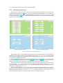
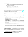
2.2.2 S-function board drivers
The source-code of the user space drivers and some kernel space routines for the two boards were
supplied by the manufacturer [12]. This gave the opportunity to make a Real-Time driver which can
interact with Simulink using LXRT. Simulink offers the possibility to use own c-code in the models
by means of S-function [10] blocks. These S-function blocks are used as board drivers to initialize the
boards and run the acquisition.
(a) Flowchart for Analog In driver.
(b) Flowchart for Analog Out driver.
Figure 2.1: Flowcharts of the S-function board drivers.
Due to LXRT only the c-code enabling the acquisition needs to be kernel calls. This implies that the
initialization procedure can be user space calls and only the code in mdlOutputs need to be kernel
calls. This has as biggest advantage that standard manufacturers source-code of the user-space drivers
can be used for initializing the boards.
In figure 2.1 the flowcharts for the Analog In 2.1(a) and Analog Out 2.1(b) show a Soft (user space)
and Hard (kernel space) Real-Time environment. The functions in Soft Real-Time are from the manufacturers user space library and those in Hard Real-Time from the kernel space routines.
There is one exception to this in the Analog In driver where the manufacturers user space drivers
use the function ioctl. This function is not compatible whit RTAI(-LXRT). Instead iopl(3), to
give input/output port permission and mmap, to map the PCI ports, has to be used. Root permission
is needed to call the function iopl(3).
The AIn and AOut drivers are very similar. The order in which initialization functions are called is
the same. The only difference are some extra functions needed to initialize the AIn driver. The most
important function in the AIn driver is AiGetAIValue and in AOut this is PdUModeAO32Write.
These two functions acquire or send data in Real-Time to or from the hardware.
CHAPTER 2. IMPLEMENTATION OF SOFT- AND HARDWARE
6
The Acquisition Delay option in the AIn Simulink GUI has a big impact on the Ain driver function
AiGetAIValue. First a command to acquire data is send to the PowerDAQ PD2-MF-16-500/16H
board. The executable starts to evaluate the next command parallel to this. However the next command
is reading the acquired data from the board, but the board is still acquiring. This results in bad readouts and/or sometimes even a shuffled channellist.
Another difference between the functions AiGetAIValue and PdUModeAO32Write is their
place in the Simulink-Time-Step loop, see figure 2.1. The function to write data is called for every
channel in the channellist individually, while the function to acquire data is called once for the complete channellist, defined in the initialization by CHLIST_ENT.
The drivers do not require any installation, merely put them in the same directory as the model
which makes use of them!
2.3 Getting started
When all the software in the appendices is installed properly, the DACS can be used. Before
starting with the checklist, beware of the limitations of External Mode. Changing a parameter that
results in a change of the model structure is not allowed. For example, changing the following is not
possible:
• The number of states, inputs or outputs of any block.
• All options in the simulation parameters menu.
• The name of the model or of any block.
• The parameters to the Fcn block
If any of these changes have to be made, new code must be generated and compiled.
2.3.1 Checklist
• Type the command modprobe pwrdaq in the console window. This loads the user space
library of the boards used in the Soft Real-Time part.
– To check if they are loaded properly type cat /proc/pwrdaq
• Then type loadrtai to load the required RTAI modules.
• In Matlab Command Window type mex uei_pd2mf_ai.c and mex uei_pd2ao_ao.c.
This is not necessary if both mex-functions already exist.
• In Simulink check the following.
– Execution mode is set to external mode, Simulation -> External.
– The discrete-time execution requires a fixed-step solver, Simulation -> Simulation
Parameters.
• When using the model the following has to be done before every run.
– In the Simulink model, select Tools -> Real-Time Workshop -> Build Model...
or use (ctrl+B) to build the RTW model.
PLEASE NOTE: When the model is build while the RTAI module is not loaded yet, the
execution of that model produces rubbish!
– Go back to the konsole and type ./"directory"/"filename" to start execution of the
model and use the options -tf 3(sec) and -w.
∗ Not specifying -tf runs the model infinitely long.
2.3. GETTING STARTED
7
∗ The option -w makes a connection to the external mode of the Simulink model.
– When -w is specified return to Simulink.
∗
∗
∗
∗
Choose Simulation -> Connect To Target.
Then Simulation -> Start Real-Time Code.
Optionally adjust parameters while the model is executed.
To stop the execution prematurely choose Simulation -> Stop Real-Time Code.
2.3.2 Simulink Graphical User Interface (GUI)
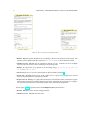
In the file Total.mdl, which can be found in the 16AI_16AO_DACS.zip archive, there is an
Analog In and Out block. The blocks contain the S-function device drivers and are shown in figure 3.2.
Used together with the two PowerDAQ boards and the custom made Connector Box in figure 3.1, up
to 16 channels Analog In and 16 channels Out can be read/send.
Predefined options for the boards When compared with the boards manuals the simulink blocks
lack a few options. For the sake of completeness this paragraph treats those options which have been
left out.
For the analog input PowerDAQ PD2-MF-16-500/16H board, which is used solely for acquiring data1 ,
these are:
• The input mode is chosen single ended. This is fixed in hardware through the connection
of the inputs in the data acquisition box.
• For clocking CL=software and CV=continuous are chosen. This combination for the
boards is typically used to acquire a single set of data points. This setting is recommended for
Real-Time control applications.
• For triggering the default option (software) is used.
• The data mode is set to fast, which is the default setting. Normal mode checks if a sample
is available to collect, this is safer but takes more time.
• The data format is fixed by the type of board and is 16 bit. for ours, see appendix B for
more information.
• The sampling method is also fixed by the board (sequential).
For the analog output board PowerDAQ PD2-AO-16/16, these are:
• The clock and trigger functionalities are combined in the update mode. There are 3 options;
this board is fixed to Single Update.
• data format is again fixed by the board (16 bit).
User defined options for the boards The options which can be set in the simulink environment are
listed below. Note that the Range in [V], Gain and SlowBit on/off options are the same for
all channels. The boards allow for setting these options for every channel separately. This slows down
the data acquisition considerably and is therefore left out.
The options as seen in figure 2.2(a) for the PowerDAQ PD2-MF-16-500/16H board are:
1 This
boards has two Analog outputs as well, but these are not supported by the S-function driver.
CHAPTER 2. IMPLEMENTATION OF SOFT- AND HARDWARE
8
(a) GUI for Analog In.
(b) GUI for Analog Out.
Figure 2.2: GUI to set options for the Simulink blocks.
• Board ID# This option should be set accordingly to the PCI slot position of the boards. The
position can be checked with the command cat /proc/pwrdaq in the Konsole window.
• Channel List Vector Can be specified in almost any way. channels can occur multiple
times and are not fixed to a strict ascending or descending order.
• Range in [V] There are 4 options to set the voltage range: [0 to 5], [0 to 10], [-5
to 5] and [-10 to 10].
• Gain Default set to 1, for more information see the PowerDAQ manual [7].
• Slow Bit on/off Can be set on or off. When set on, it gives leaves a larger time interval
between acquiring data for subsequent channels
• Acquisition Delay in [ns] Value for the time interval between the command to acquire
data and the command to read this data from the board. Adjusting this parameter is a comparative assessment between lower achievable sample rates and incorrect acquisition.
And in figure 2.2(b) the options for the PowerDAQ PD2-AO-16/16 board are:
• Board ID# The same as for the Analog In board.
• Channel List Vector Also the same.
Chapter 3
Performance of the DACS
To give an idea of what the DACS is capable of, in this chapter the performance is evaluated by
means of experiments. Before any experiment can begin, a Connector Box (CBox) has to be connected.
The CBox has 16 coaxial female connectors for Analog In and 16 for Analog Out. They are all connected in single-ended mode to the PowerDAQ boards in the PC. To accommodate the experiments,
the Analog In channels are connected to the Analog Out channels, see figure 3.1
Figure 3.1: Custom made Connector Box for the PowerDAQ boards.
In Simulink the two S-function board driver blocks are put together in one model (figure 3.2). The
model can easily be adjusted to put a sine wave or a constant signal on the analog outputs. These
signals can be the same for all channels or can have a small amplitude difference. The analog input
values from the CBox inputs can be compared with the original signals. Both send and acquired data
is saved to the workspace for further calculations.
In the remaining sections, the performance and accuracy of the boards is treated. This is merely to
give an idea of what is working correctly and what to improve. Every set of channels can be optimized
for performance. For example if the model is executed on the same PC, logically a 1 AIn 1 AOut model
will achieve a far higher sample rate than a 16 AIn 16 AOut model.
When performing an experiment, an external oscilloscope should be used to verify if the model
executes Real-Time or not. For an unknown reason the target does not always correctly indicate missed
interrupts. With the scope this becomes apparent because a signal is transmitted for e.g. 3.5[s] instead
of the intended 3.0[s]. This problem should be resolved when newer versions of the software are
installed and is therefore ignored.
9
CHAPTER 3. PERFORMANCE OF THE DACS
10
1
a
[S0]
[S0]
0
0
[S0]
1
b
[S1]
[S1]
1
1
[S1]
Constant3
c
[S2]
[S2]
2
2
[S2]
d
[S3]
[S3]
3
3
[S3]
e
[S4]
[S4]
4
4
[S4]
f
[S5]
[S5]
5
5
[S5]
g
[S6]
[S6]
6
6
h
[S7]
[S7]
7
Constant2
Sine Wave2
Sine Wave3
i
[S8]
[S8]
8
PowerDaq PD2 AO
Analog Output
PowerDaq PD2 MF
Analog Input
[S6]
7
[S7]
Ain
8
Aout
[S8]
To Workspace
j
[S9]
[S9]
9
k
[S10]
[S10]
10
10
[S10]
l
[S11]
[S11]
11
11
[S11]
m
[S12]
[S12]
12
12
[S12]
n
[S13]
[S13]
13
13
[S13]
o
[S14]
[S14]
14
14
[S14]
p
[S15]
[S15]
15
15
[S15]
9
PD2_AO_Series1
[S9]
To Workspace1
PD2_MF_Series1
Figure 3.2: Simulink model used in the experiments.
3.1 Performance
When a model is executed for the specified time period, it still takes about 4.5[s] to shut down the
Real-Time process. Furthermore the first few measurements are incorrect, due to initialization effects.
Depending on sample rate and the channellist, this can vary between 0 − 150 points.
When shooting for the highest possible performance for a certain set of channels, the sample rate
and Acquisition Delay need to be optimized. The sample rate should be chosen as high as possible.
The Acquisition Delay should be lowered until the read-out becomes rubbish.
A good procedure to check the performance of a certain set of channels is:
• Always check with a scope whether the model execution stays Real-Time.
• The desired set of channels and/or sample rate is known.
• When a maximal sample rate is desired.
– Configure the model in figure 3.2 according to the set of channels.
– Determine maximum sample rate, without loosing the Real-Time property (scope) or have
the PC not responding.
– Check if the read out of the channels is correct, adjust Acquisition Delay accordingly.
– If the Acquisition Delay is adjusted, determine the sample rate once more.
– It goes without saying that in the next step a sample rate smaller than the determined
maximum should be chosen.
• When the desired sample rate is known
– Configure the model in figure 3.2 according to the set of channels and the desired sample
rate.
– Write down the minimal value for the Acquisition Delay before the read-outs become rubbish.
– Increase the Acquisition Delay until the Real-Time property (scope) is lost, and write this
value down.
– Subtracting these two values gives the process-time available for controller calculation.
Knowing the sample rate, the percentage of the total time available for the controller can
be calculated.
3.2. ACCURACY
11
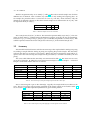
With the Acquisition Delay set to 10000[ns], table 3.1 shows the maximal sample rates for three
different sets of channels. This is without any controller, so only sending and acquiring data. As
an example, the procedure above is carried out for a set of 7 AIn and 7 AOut channels. Only the
desired set of channels is known, so first the maximal sample rate is determined to be 16[kHz] with
an Acquisition Delay of 3000[ns].
N o of channels
Sample rate [kHz]
1
22.5
8
15
16
9
Table 3.1: Maximal sample rate for sets of channels.
Next a sample rate of 10[kHz] is chosen. The minimal Acquisition Delay stays 3000[ns]. The maximum is about 40000[ns] without loosing the Real-Time property or having the PC not-responding.
This leaves 37[µs] in a loop of 100[µs] (10[kHz]) for a controller computation, so almost 40[%]! This
could be expected, because the chosen sample rate is about 60[%] of the maximal sample rate.
3.2 Accuracy
The Simulink model will execute with discrete time-steps. This implies that the Analog Out port(s)
are sending a sample while the Analog In port(s) are acquiring the previous sample. This time delay
will work the other way around in a real system. Where first some measurement signal will be acquired, and in the next time-step that sample will be processed by a controller and send by the Out
port(s).
The errors which illustrate this time delay are summarized in table 3.2. The same sine wave was
put on all 16 channels. By taking the error between AOut sample k and AIn sample k−1 instead of
sample k for the both of them, the error is reduced.
Sine wave [Hz]
N o of channels
Sample freq [kHz]
Sample shift
1 [V]
2 [V]
5 [V]
4
16
0.5
-
yes
4
16
1.0
-
[-0.070, 0.050]
yes
50
1
10.0
-
[-0.025, 0.010]
[-0.045, 0.030]
yes
[-0.025, 0.010]
[-0.070, 0.035]
[-0.040, 0.010]
[-0.120, 0.100]
[-0.035, 0.020]
[-0.270, 0.250]
[-0.100, 0.040]
[-0.070, 0.055]
[-0.035, 0.020]
[-0.100, 0.065]
[-0.050, 0.015]
[-0.150, 0.135]
[-0.100, 0.040]
[-0.200, 0.160]
[-0.080, 0.035]
Table 3.2: Error intervals [min, max] illustrating the phase shift due to time-steps.
Next a constant signal is put on the channel(s). Logically, the sample shift has no effect on the
error. The error increases with increasing amplitude of the signals, which can be found in table 3.2
too. In section 3.3 possible explanations/solutions are given for this problem.
N o of channels
Time-step [kHz]
Sample shift
2 [V]
5 [V]
1
10.0
[-0.006, 0.010]
[0.017, 0.035]
yes
16
1.0
-
yes
[-0.006, 0.010]
[-0.007, 0.020]
[-0.007, 0.020]
[0.017, 0.035]
[0.015, 0.045]
[0.015, 0.045]
Table 3.3: Error intervals [min, max] when applying a constant signal to sets of channels.
12
CHAPTER 3. PERFORMANCE OF THE DACS
3.3 Discussion
Once again it is stressed that the experiments described above are only mend to give a first impression. No hard conclusion can be drawn, merely some guesses of what to do to improve the performance and accuracy, because the DACS is not completely finished. Any change to the DACS will
have an effect on the performance and accuracy. So a detailed survey is only useful after completion.
Still it may be clear that the errors are considerable and increasing with the amplitude of the
signals. First of all, the direct connection of the input and output as depicted in figure 3.1 may cause
ground-loops. This could be the reason for the large amount of noise on even small amplitude signals.
During the building process of the CBox, there was some discussion about connecting the ports
single-ended or differential. The connector pcb in the CBox was soldered three times because of this.
As a result the connector pcb short-circuited twice already and is expected to do so in the future. Of
course this can have a negative influence on the signals as well, but not on all signals.
Finally, the PowerDAQ PD2-MF-16-500/16H was manufactured on 01-Jan-2003 and calibrated
on 21-Nov-2003 and PowerDAQ PD2-AO-16/16 respectively on 01-Oct-2003 and 24-Nov-2003. The
manual of the PowerDAQ PD2-AO-16/16 board recommends a calibration every year. There is a PowerDAQ software tool under windows to recalibrate the board, however it requires a high-precision
voltage source. Another option could be to adjust the equation which calculates the voltage from the
rawbuffer. Of course before any of this takes place the errors have to be identified as being deterministic.
Chapter 4
Conclusions and Recommendations
Conclusions Two Simulink S-function driver blocks for the PowerDAQ boards have been realized,
which make Hard Real-Time execution of Simulink models possible on a Linux RTAI-LXRT platform.
Together with the custom made Connector Box, a rapid control prototyping system is constructed.
Using the standard user space library functions, the PowerDAQ PD2-AO-16/16 has a maximal
sample rate of 100[kS/s] and the PowerDAQ PD2-MF-16-500/16H of 500[kS/s]. The achieved sample
rates have improved considerably for the LXRT platform in comparison to the original drivers, by using
direct kernel calls to communicate with the boards. However, the maximal sample rates of the DACS
is in general limited by the PC’s processor. As stated earlier, the same processor power is used in a 1
channel or a 16 channel configuration, so performance depends heavily on the number of channels
and the controller complexity.
Recommendations The DACS is not completely ready to be implemented into a real set-up. Unfortunately, an error remained on the signals, consisting of noise, DC error and a gain error! Either there’s
a ground-loop, noise sensitive connections in the Connector Box or, most likely, the boards need to be
recalibrated. Also the missed-interrupt issue from chapter 3 page 9 still needs to be solved. This is
probably as simple as updating software. Of course for every set-up a set of channels and sample rate
have to be chosen/optimized!
Finally, when attempting to build a DACS on the Linux RTAI-LXRT platform the following should
be considered. Basic knowledge about Linux and RTAI and programming in c-code is expedient.
Advanced knowledge about these subjects is a definite pro. Be aware that the PowerDAQ boards in
this report work with I/O memory mapping while other PCI boards communicate with I/O ports.
Remember that any board will need specific drivers and for a RTAI implementation, only kernel
calls are allowed. Unfortunately these are not supplied by the manufacturer. This may be a criterium
when buying boards. An alternative can be the Comedi project [1]. Within this project, currently a
wide selection of supported boards can be found.
At the time the PowerDAQ boards were purchased, the Comedi project only gave a limited choice
of supported hardware but this has grown since the start of this project. So it is recommended to
either buy a board for which a Comedi driver is already available or write a driver yourself, according
to the conventions of the Comedi project.
13
14
CHAPTER 4. CONCLUSIONS AND RECOMMENDATIONS
Appendix A
S-function C-code
A.1 Analog In file
/*
Analog input S-function for:
United Electronic Industries
PowerDAQ board type: PD2-MF-16-500/16H
Input Fifo size:
1024 samples
CL FIFO Size:
256 entries
Output Fifo size:
2048 samples
Mfg. date:
01-JAN-2003
Cal. date:
21-NOV-2003
Firmware type: MFx rev: 3.31/30819
(c) Frederik Klomp,
Februari
2005
*/
#define S_FUNCTION_NAME uei_pd2mf_ai #define S_FUNCTION_LEVEL 2
#include "simstruc.h" #include <math.h>
#define NPARAMS
6 #define BoardID
ssGetSFcnParam(S,1) #define Range
ssGetSFcnParam(S,3) #define SlowBit
ssGetSFcnParam(S,5)
ssGetSFcnParam(S,0) #define ChannelList
ssGetSFcnParam(S,2) #define GainSet
ssGetSFcnParam(S,4) #define AcquiDelay
#ifndef MATLAB_MEX_FILE #include <stdio.h> #include <stdlib.h> #include <stdint.h>
#include <fcntl.h> #include <sys/io.h> #include <sys/mman.h> #include <sys/types.h>
#include <sys/time.h> #include <unistd.h> #include "win_sdk_types.h" #include "rtai.h"
#include "rtai_sched.h" #include "powerdaq.h" #include "powerdaq32.h" #endif
int i;
#ifndef MATLAB_MEX_FILE
static PWRDAQ_PCI_CONFIG pciConfig;
static DWORD RangeTypes;
int j;
int retVal = 0;
int board;
// board number to be used for the AI operation
static int Handle;
// board Handle
void* bar0Address;
int mem_fd;
unsigned long aiCfg;
int scanSize;
int range;
static double BitWeight;
static double Displacement;
static int Gain;
static int Delay;
//FUNCTIONS
#define CHAN(c)
#define GAIN(g)
((c) & 0x3f)
(((g) & 0x3) << 6)
15
APPENDIX A. S-FUNCTION C-CODE
16
#define SLOW
(1<<8)
#define CHLIST_ENT(c,g,s)
(CHAN(c) | GAIN(g) | ((s) ? SLOW : 0))
unsigned long AiGetAIValue(int scanSize, unsigned long*
int AiDrvDSPCmd(int command);
unsigned long AiDrvDSPRead();
buffer, int sleep);
inline void AiDrvWrite(unsigned long offset, unsigned long data)
{
unsigned long *reg = (unsigned long*)(bar0Address + offset);
*reg = data;}
inline unsigned long AiDrvRead(unsigned long offset)
{
unsigned long *reg = (unsigned long*)(bar0Address + offset);
return *reg;}
unsigned long AiGetAIValue(int scanSize, unsigned long* rawbuffer, int sleep)
{
// tell the board to acquire one scan
AiDrvDSPCmd(PD_AISWCLSTART);
if(AiDrvDSPRead() == 1)
{
// read every samples in the scan
rt_busy_sleep(sleep);
for(i=0; i<scanSize;i++)
{
AiDrvDSPCmd(PD_AIGETVALUE);
rawbuffer[i] = AiDrvDSPRead();}
return 0;
}
return -1;}
int AiDrvDSPCmd(int command)
{
AiDrvWrite(PCI_HCVR, (1L | command));
return 0;}
unsigned long AiDrvDSPRead()
{
return AiDrvRead(PCI_HRXS);}
#endif
static void mdlInitializeSizes(SimStruct *S) {
ssSetNumSFcnParams(S,NPARAMS);
ssSetNumContStates(S,0);
ssSetNumDiscStates(S,0);
ssSetNumInputPorts(S,0);
ssSetNumOutputPorts(S,mxGetN(ChannelList));
for (i = 0; i < mxGetN(ChannelList); i++) {
ssSetOutputPortWidth(S,i,1);}
ssSetNumSampleTimes(S,1);
ssSetNumRWork(S,0);
ssSetNumIWork(S,0);
ssSetNumPWork(S,0);
ssSetNumDWork(S,0);
ssSetNumModes(S,0);
ssSetNumNonsampledZCs(S,0);
#ifndef MATLAB_MEX_FILE
board = (int)mxGetPr(BoardID)[0]-1;
range = (int)mxGetPr(Range)[0];
Gain = 1;
Delay = (int)mxGetPr(AcquiDelay)[0];
Handle = 0;
scanSize = mxGetN(ChannelList);
if (range == 1){
RangeTypes = 0; BitWeight = 0.000076295; Displacement = 0;}
else if (range == 2){
RangeTypes = AIB_INPRANGE; BitWeight = 0.000152590; Displacement = 0;}
else if (range == 3){
RangeTypes = AIB_INPTYPE; BitWeight = 0.000152590; Displacement = -5;}
else if (range == 4){
RangeTypes = AIB_INPTYPE | AIB_INPRANGE; BitWeight = 0.000305180; Displacement = -10;}
aiCfg = AIB_CVSTART0 | AIB_CVSTART1 | RangeTypes;
A.1. ANALOG IN FILE
17
unsigned int ChLst[scanSize];
for (i = 0; i < scanSize; i++) {
ChLst[i]= CHLIST_ENT((int)mxGetPr(ChannelList)[i],(int)mxGetPr(GainSet)[0]-1,(int)mxGetPr(SlowBit)[0]);}
Handle = PdAcquireSubsystem(board, BoardLevel, 1);
if(Handle <0)
{
printf("AI: PdAcquireSubsystem error %d\n", Handle);}
retVal = PdGetPciConfiguration(Handle, &pciConfig);
if(retVal != 0) {
printf("AI: PdGetPciConfiguration error %d\n", retVal);}
retVal = _PdAInSetCfg(Handle, aiCfg, 0, 0);
if (retVal < 0) {
printf("AI: _PdAInSetCfg error %d\n", retVal);}
retVal = _PdAInSetChList(Handle, scanSize, ChLst);
if (retVal < 0) {
printf("AI: _PdAInSetChList error %d\n", retVal);}
retVal = _PdAInEnableConv(Handle, TRUE);
if (retVal < 0) {
printf("AI: _PdAInEnableConv error %d\n", retVal);}
retVal = iopl(3);
if(retVal != 0) {
printf("AI: iopl failed, make sure you have root permission\n");}
if((mem_fd = open("/dev/mem", O_RDWR)) < 0)
{
printf("AI: open(/dev/mem) error %d\n", mem_fd);}
bar0Address = mmap(0, 16384, PROT_READ | PROT_WRITE, MAP_SHARED, mem_fd, pciConfig.BaseAddress0);
if(bar0Address == (void*)-1 || bar0Address == NULL) {
printf("AI: mmap error %d\n", (int)bar0Address);}
retVal = _PdAInSwStartTrig(Handle);
if (retVal < 0) {
printf("AI: _PdAInSwStartTrig failed with %d.\n", retVal);}
#endif
}
static void mdlInitializeSampleTimes(SimStruct *S) {
ssSetSampleTime(S,0,CONTINUOUS_SAMPLE_TIME);
ssSetOffsetTime(S,0,0.0);
}
static void mdlOutputs(SimStruct *S, int_T tid) {
real_T *y;
#ifndef MATLAB_MEX_FILE
unsigned long* rawbuffer[16]; //change if more channels are needed
double buffer[16]; //change if more channels are needed
AiGetAIValue(scanSize, rawbuffer, Delay);
for(i=0; i < scanSize; i++) {
y=ssGetOutputPortRealSignal(S,i);
y[0]=(((unsigned long)rawbuffer[i] ^ 0x8000) * BitWeight + Displacement)/Gain;
}
#endif }
static void mdlTerminate(SimStruct *S) { #ifndef MATLAB_MEX_FILE
munmap(bar0Address, mem_fd);
close(mem_fd);
retVal = _PdAInReset(Handle);
if (retVal < 0) {
printf("AI: PdAInReset error %d\n", retVal);}
retVal = PdAcquireSubsystem(Handle, BoardLevel, 0);
if (retVal < 0) {
printf("AI: PdReleaseSubsystem error %d\n", retVal);}
#endif }
18
#ifdef
APPENDIX A. S-FUNCTION C-CODE
MATLAB_MEX_FILE #include "simulink.c" #else #include "cg_sfun.h" #endif
A.2. ANALOG OUT FILE
19
A.2 Analog Out file
/*
Analog output S-function for:
United Electronic Industries
PowerDAQ board type:
PD2-AO-16/16
Output Fifo size:
2048 samples
Mfg. date:
01-Oct-2003
Cal. date:
24-Nov-2003
Firmware type: AO rev: 3.31/30819
(c) Maurice Schneiders, September 2004
(c) Frederik Klomp,
Februari 2005
*/
#define S_FUNCTION_NAME uei_pd2ao_ao #define S_FUNCTION_LEVEL 2
#include "simstruc.h" #include <math.h>
#define NPARAMS
2 #define BoardID
ssGetSFcnParam(S,1)
ssGetSFcnParam(S,0) #define ChannelList
#ifndef MATLAB_MEX_FILE #include <stdio.h> #include <stdlib.h> #include <stdint.h>
#include <fcntl.h> #include <sys/io.h> #include <sys/mman.h> #include <sys/types.h>
#include <sys/time.h> #include <unistd.h> #include "win_sdk_types.h" #include
"powerdaq.h" #include "powerdaq32.h" #endif
static int i;
#ifndef MATLAB_MEX_FILE
static void* bar0Address; static int mem_fd; static int Handle; static int retVal = 0;
static DWORD value; static DWORD aoCfg = 0; static PWRDAQ_PCI_CONFIG pciConfig;
inline void PdUModeDrvWrite(unsigned long offset, unsigned long data)
unsigned long *reg = (unsigned long*)(bar0Address + offset);
*reg = data;}
{
inline unsigned long PdUModeDrvRead(unsigned long offset)
{
unsigned long *reg = (unsigned long*)(bar0Address + offset);
return *reg;}
int PdUModeDrvDSPWrite(unsigned long data)
PdUModeDrvWrite(PCI_HTXR, data);
return 0;}
{
int PdUModeDrvDSPCmd(int command)
{
PdUModeDrvWrite(PCI_HCVR, (1L | command));
return 0;}
unsigned long PdUModeDrvDSPRead()
{
return PdUModeDrvRead(PCI_HRXS);}
int PdUModeDrvDIO256Write(int cmd, unsigned long val)
unsigned long ret;
{
// Send write command and receive acknowledge
PdUModeDrvDSPCmd(PD_DI0256WR);
ret = PdUModeDrvDSPRead();
if (ret != 1) return 0;
// Write command
PdUModeDrvDSPWrite(cmd);
// Write parameter and rcv ack
PdUModeDrvDSPWrite(val);
ret = PdUModeDrvDSPRead();
return (ret)?1:0;}
int PdUModeAO32Write(unsigned short wChannel, unsigned short wValue)
{
return PdUModeDrvDIO256Write((wChannel & 0x7F)|AO32_WRPR|AO32_BASE, wValue);}
#endif
static void mdlInitializeSizes(SimStruct *S) {
ssSetNumSFcnParams(S,NPARAMS);
ssSetNumContStates(S,0);
ssSetNumDiscStates(S,0);
ssSetNumOutputPorts(S,0);
APPENDIX A. S-FUNCTION C-CODE
20
ssSetNumInputPorts(S,mxGetN(ChannelList));
for (i = 0; i < mxGetN(ChannelList); i++) {
ssSetInputPortWidth(S,i,1);
}
ssSetNumSampleTimes(S,1);
ssSetNumRWork(S,0);
ssSetNumIWork(S,0);
ssSetNumPWork(S,0);
ssSetNumDWork(S,0);
ssSetNumModes(S,0);
ssSetNumNonsampledZCs(S,0);
#ifndef MATLAB_MEX_FILE
Handle=PdAcquireSubsystem((int)mxGetPr(BoardID)[0]-1, BoardLevel, 1);
if(Handle < 0) {
printf("AO: PdAcquireSubsystem failed\n");
exit(EXIT_FAILURE);}
retVal = PdGetPciConfiguration(Handle, &pciConfig);
if(retVal != 0) {
printf("AO: PdGetPciConfiguration error %d\n", retVal);}
_PdAOutSetCfg(Handle, aoCfg, 0);
if (retVal < 0) {
printf("AO: _PdAOutSetCfg error %d\n", retVal);
exit(EXIT_FAILURE);}
retVal = iopl(3);
if(retVal != 0) {
printf("AO: iopl failed, make sure you have root permission\n");}
if((mem_fd = open("/dev/mem", O_RDWR)) < 0) {
printf("AO: open(/dev/mem) error %d\n", mem_fd);}
bar0Address = mmap(0, 16384, PROT_READ | PROT_WRITE, MAP_SHARED, mem_fd, pciConfig.BaseAddress0);
if(bar0Address == (void*)-1 || bar0Address == NULL) {
printf("AO: mmap error %d\n", (int)bar0Address);}
_PdAOutSwStartTrig(Handle);
if (retVal < 0) {
printf("AO: PdAOutSwStartTrig failed with %d.\n", retVal);
exit(EXIT_FAILURE);}
#endif }
static void mdlInitializeSampleTimes(SimStruct *S) {
ssSetSampleTime(S,0,CONTINUOUS_SAMPLE_TIME);
ssSetOffsetTime(S,0,0.0);
}
static void mdlOutputs(SimStruct *S, int_T tid) {
InputRealPtrsType uPtrs;
#ifndef MATLAB_MEX_FILE
for(i=0; i < mxGetN(ChannelList) ; i++) {
uPtrs = ssGetInputPortRealSignalPtrs(S,i);
int ChannelNumber = mxGetPr(ChannelList)[i];
unsigned long value = ((*uPtrs[0])+10.0)/20.0*0xFFFF;
PdUModeAO32Write(ChannelNumber, value);
}
#endif }
static void mdlTerminate(SimStruct *S) { #ifndef MATLAB_MEX_FILE
munmap(bar0Address, mem_fd);
close(mem_fd);
retVal = _PdAOutReset(Handle);
if (retVal < 0) {
printf("AO: PdAOutReset error %d\n", retVal);}
retVal = _PdAO32Reset(Handle);
if (retVal < 0) {
printf("AO: PdAAO32Reset error %d\n", retVal);}
A.2. ANALOG OUT FILE
PdAcquireSubsystem(Handle, BoardLevel, 0);
if (retVal < 0) {
printf("AO: PdReleaseSubsystem error %d\n", retVal);}
#endif }
#ifdef
MATLAB_MEX_FILE #include "simulink.c" #else #include "cg_sfun.h" #endif
21
APPENDIX A. S-FUNCTION C-CODE
22
11
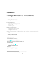
Appendix B
Listings of hardware and software
Listing of hardware used:
PC Dell OptiPlex GX270
R Pentium°
R 4, 2.6 GHz
CPU Intel°
RAM 512 MB
HD IDE, 19.5 GB
Boards PowerDAQ board type:
Analog In PD2-MF-16-500/16H
Analog Out PD2-AO-16/16
monitor IIyama Vision Master 400 (horizontal sync range: 27-96 kHz, vertical sync range: 50-160
Hz)
Listing of software used:
Matlab version 6.1 R12
Real-Time Workshop version 4.0
Wintarget [4] for RTAI, using Matlab 6.1
RTAI version 3.0r3, using patched Linux kernel 2.4.24
Linux RTAI LXRT
Scheduling rtai_lxrt1
Real-time processes rtai_hal
Knoppix 3.3
gcc version 3.3.5 (debian 1:3.3.5-8)
1 Makes
use of modules rtai_netrpc, rtai_msg, rtai_mbx, rtai_sem and rtai_fifod.
23
24
APPENDIX B. LISTINGS OF HARDWARE AND SOFTWARE
Appendix C
Installation of the Linux OS and extra
software
C.1 Linux OS
The Knoppix 3.3 distribution is used, which can be installed from CD. Put the CD in the drive and
wait for Knoppix to start. Next, start the konsole window and type knx-hdinstall, which will start
the harddisk installation. Click through the options or use the extensive installation guide [3].
C.2 GCC 3.2
To be able to install version 3.2 of gcc (C-compiler), first a new apt-source has to be added to the
system. Use an text-editor to open the file /etc/apt/sources-list. Add the lines:
deb http://ftp.nl.debian.org/debian/ testing main
deb-src http://ftp.nl.debian.org/debian/ testing main
Save the file and close the text-editor. Now open a console window, e.g. Konsole. You can find this
under Start → System → Shell. give the command
apt-get update1
this updates the list of available packages with the added apt-sources.
Next a few packages (these versions or higher) can be added to the system, use the command
apt-get install #NAME#
where you have to fill in every item of the following list for #NAME#:
• gcc-3.2 → also update glibc
• g++-3.2
• g77-3.2
• mesag-dev
• libfltk1-dev
• libncurses5-dev
• kdm (optional)
1 This
can possibly generate an error: Reading package list /etc/apt/apt.conf add line: APT::Cache-limit 10000000
25
26
APPENDIX C. INSTALLATION OF THE LINUX OS AND EXTRA SOFTWARE
Doing this, the listed are packages being updated and being installed. When asked, choose to
restart services. While installing kdm you have to choose the standard “display manager”. Choose the
option kmd.
The new compilers gcc and g++ are not operational yet. First a symbolic link to the compiler has
to be changed. Realize this with:
cd /usr/bin
ln -s -f gcc-3.2 gcc
ln -s -f g++-3.2 g++
To make sure the correct compilers are in use by the system give the command:
gcc -v
Other options to install extra software are dselect and the graphical program Package Manager.
This will update all the packages to the “testing” distribution. This is very time consuming and has
not be tested thoroughly.
C.3 Internet
To make use of the internet connection from the DCT-lab, the proxy settings of the internet
browser, e.g. Mozilla have to be set. Without the correct setting it is only possible to surf within
the TU/e domain.
Start Mozilla (e.g. with mozilla &) and open the Preferences in the menu Edit. Go to category Advanced/Proxies and manually fill in the http-proxy-server as: proxy.wfw.wtb.tue.nl
and port 80.
Any other internet browser will need similar settings.
Appendix D
Matlab 6.1
D.1 Preparation
Before we can start installing Matlab 6.1, some settings in Debian need to be changed. First of all
it has to be possible to start programs from CD. Open /etc/fstab in any text-editor. In the same
line as /dev/cdrom add the option exec.
/dev/cdrom /cdrom iso9660 ro,user,noauto,exec 0 0
It is now possible to mount a CD with the command mount /dev/cdrom.
Next the package locales has to be reconfigured with the command:
dpkg-reconfigure locales
Choose for locales:
• en_US ISO-8859-1
• en_US ISO-8859-15 ISO-8859-15
• en_US.UTF-8 UTF-8
Leave the standard locale as it is with leave alone.
D.2 Installation
Now we can start installing Matlab 6.5. Mount the Matlab-CD with the command:
mount /dev/cdrom
Copy the license-file to the installation directory so we can make use off the stand-alone license. This
can be any directory, hereafter we use /usr/local/matlab6p1. Create this and a subdirectory
with
mkdir /usr/local/matlab6p1
mkdir /usr/local/matlab6p1/etc
and copy from CD the file license.dat to /usr/local/matlab6p1/etc with
cp /cdrom/crack/license.dat /usr/local/matlab6p1/etc/
Next start the Matlab installer with
/cdrom/install &
Use for root directory of the Matlab installation /usr/local/matlab6p5. Customize the parts you
want to be installed, but choose at least:
• Matlab
• Matlab Toolbox
• Matlab Kernel
27
APPENDIX D. MATLAB 6.1
28
• Simulink
• Matlab Compiler
• Real-time Workshop
• FLEXm
Check “Create symbolic links to Matlab and mex scripts” and choose /usr/local/bin as path. The
display license number 0 is correct.
D.3 Configuration
After installation the FLEXm server should start automatically. This requires a startup script, which
has to be copied:
cp /usr/local/Matlab6p1/etc/rc.lm.glnx86 /etc/init.d/lm.glnx86
An option still needs to be changed in the startup script. Therefor open it in any text-editor, e.g.
/etc/init.d/lm.glnx86 and change the following line:
/etc/lmboot_TWM12 -u username && echo ’Matlab_lmgrd’ to
/etc/lmboot_TWM12 -u pc35 && echo ’Matlab_lmgrd’
Next activate the script with:
update-rc.d lm.glnx86 defaults
After rebooting the FLEXm server should be active and Matlab can be started with the command:
Matlab &
The &-operator after a command executes the program in the background. This leaves the console
window open for new commands.
Appendix E
RTAI
In this appendix it is assumed you are logged in as root. You will need it at least for installing the
kernel and RTAI.
E.1 Requirements for RTAI
The required software for RTAI can either be copied from the CD or be downloaded from internet.
After copying the source-code onto the computer in any of the two ways it still needs to be unpacked.
Downloading the software from the internet The kernel source-code can also be downloaded:
http://www.kernel.org/pub/linux/kernel
For this version of RTAI use kernel 2.4.24. Go to v2.4 and download linux-2.4.24.tar.bz2 to
the directory /usr/src.
For downloading the RTAI source-code go to:
http://www.rtai.org.
Click Download RTAI and then Download Area. Now download rtai-3.0r3.tgz to the directory /usr/src.
Unpacking the software Unpack the two archives in /usr/src with:
cd /usr/src
tar --bzip2 -xvf linux-2.4.24.tar.bz2
tar -xvzf rtai-3.0r3.tgz
E.2 Compiling the kernel
To make RTAI available the kernel needs to be patched. This requires changing some parts of the
kernel source-code. Go to the directory where the Linux code has been unpacked.
cd /usr/src/linux-2.4.24
Patch the kernel using
patch -p1 < /usr/src/rtai-3.0r3/patches/patch-2.4.24-rthal5g
Next configure the kernel, it is best to use the graphical menu.
make xconfig
Now we can make use of the provided configuration file (Load Configuration from File. The
location of this file is /cdrom/kernelconfig. When this configuration is not used, you should pay
attention to the following:
• Loadable module support
29
APPENDIX E. RTAI
30
– Set version information on all module symbols, choose N
• Processor type and features
– Processor family, choose Pentium-Pro/Celeron/Pentium-II
– Real-Time Hardware Abstraction Layer, choose Y
– Local APIC support on uniprocessor, choose Y
• Networking options
– Packet socket, choose Y (or else the DHCP will not work)
– Socket filtering, choose Y (or else the DHCP will not work)
• Network device support
– Ethernet (10 or 100 Mbit)
∗ 3COM Cards, choose Y
∗ 3c590/3c900..., choose Y
• File systems
– Microsoft Joliet CDROM extensions, choose Y
Close xconfig (safe and exit). Execute the following sequence of commands:
make dep
make bzImage
make modules
make modules_install1
When asked, answer y to starting lilo. Reboot the PC and the kernel should be up and running.
E.3 Installing RTAI
First change the source and installation directory. Go to the directory by typing
cd ./usr/src/rtai-3.0r3 in the konsole. Then give the command menuconfig, a new window opens. Choose general and then change the installation directory to /usr/realtime and the
source directory to /usr/src/linux-2.4.24. Exit the window and save the changes made.
Then simply follow the manual located at /usr/src/rtai-3.0r3 and named INSTALL.
E.4 RTAI Target Real Time Workshop
To switch to the use of Real-Time applications, the relevant files are libtimer.c, buildlib,
ml2, timer.h and are zipped together with the s-functions and
Simulink blocks. Simply run the buildlib-program and everything should work.
There is an exception to this, if Matlab has been (or will be) re-installed, you need a new version of
wt_main.c (also on the Linux-software CD) that is located in the /usr/local/matlab6p1/rtw/c/wintarget
directory (so just delete and replace the file).
1 This command can result in errors. If so, clear all the modules in /lib/modules/2.4.24-adeos and compile them again
make install
Bibliography
[1]
Linux COntrol and MEasurement Device Interface, "Comedi homepage", www.comedi.org.
[2]
dSPACE GmbH, "dSPACE homepage", www.dspace.com.
[3]
Knoppix 3.3 installation guide, kookboek.knoppix.nl/kk33hd.htm.
[4]
Dr. Ir. M.J.G. v.d. Molengraft is an assistant professor in the Control Systems Technology group
of the Mechanical Engineering Department of Eindhoven University of Technology. TUeDACS
support pages: http://www.tuedacs.nl/ or
http://www.dct.tue.nl/home_of_wintarget.htm.
[5]
National Instruments Corporation, "NI homepage", www.ni.com.
[6]
W.T. Oud, "Implementatie Real-Time Linux", Unnumbered internal document, Eindhoven University of Technology.
[7]
Manual for the Analog Input board PowerDAQ PD2-MF-16-500/16H:
http://www.ueidaq.com/pdf/manuals/pd2mf_manual.pdf,
Manual for the Analog Output board PowerDAQ PD2-AO-16/16:
http://www.ueidaq.com/pdf/manuals/pd2ao_manual.pdf.
[8]
Quanser Inc., "Quanser, innovate, educate homepage", www.quanser.com.
[9]
RTAI project founded by the Department of Aerospace Engineering of Politecnico di Milano
(DIAPM), "RTAI homepage", www.rtai.org.
[10] Manual for writting S-functions,
www.mathworks.com/access/helpdesk/help/toolbox/simulink/sfg/.
[11] Ing. P. Soetens is a research fellow in the Department of Mechanical Engineering of the
Katholieke Universiteit Leuven, e-mail: [email protected].
[12] United Electronic Industries, Inc., "Powerdaq boards homepage",
http://www.ueidaq.com/.
31