Download Campbell PC208 Instruction manual

Measurements of Sap Flow
by the Heat-Pulse Method.
An Instruction Manual for the HPV system
August, 1998
Steve Green
HortResearch Institute
Private Bag 11-030
Palmerston North
New Zealand
Summary
Heat-pulse techniques can be used to measure sap flow in plant stems with minimal
disruption to the sap stream (Swanson and Whitfield, 1981; Cohen et al., 1981; Green and
Clothier, 1988). The measurements are reliable, use inexpensive technology, provide a
good time resolution of sap flow, and they are well-suited to automatic data collection
and storage. Sequential or simultaneous measurements on numerous trees are possible,
permitting the estimation of transpiration from whole stands of trees.
The HPV system described here is based on the ‘compensation’ Heat-Pulse method
(Swanson and Whitfield, 1981) and comprises a set of probes and associated electronics
connected to a data logger (model CR10, Campbell Scientific Inc., Utah, USA). Included
with the system is a set of computer programs to CAPTURE and ANALYZE the heatpulse measurements, which are recorded automatically by the data logger. The purpose of
this document is to describe how to successfully install and operate the HPV system.
2
Contents
Summary
1.
..
..
..
..
..
..
..
..
..
2
Background and Theory
..
..
..
..
..
..
5
1.1
The origin of heat-pulse
..
..
..
..
..
5
1.2
Idealized heat-pulse theory
..
..
..
..
..
5
1.3
Wound corrections to the heat-pulse theory ..
..
..
6
1.4
Converting heat-pulse velocity to sap flow
..
..
..
10
1.5
Measuring the volume fractions, FM and FL ..
..
..
10
1.6
Estimating volumetric sapflow
..
11
..
..
..
..
12
3.
Connecting up the logger and getting it going
..
..
..
13
3.1
Assembling the necessary hardware ..
..
..
..
13
3.2
Connecting the HPV unit to the datalogger ..
..
..
13
Installing the heat-pulse probes
..
..
Instrumentation
5.
..
..
2.
4.
..
..
..
..
..
..
..
14
4.1
Checking if the probes are OK
..
..
..
..
14
4.2
Procedure for installing probes
..
..
..
..
15
4.3
Testing if everything is working
..
..
..
..
16
Installing the datalogger software
..
..
..
..
..
16
5.1
Files in A:\LOGGER ..
..
..
..
..
..
16
5.2
Files in A:\CAMP
..
..
..
..
..
17
5.3
Downloading programs to the logger ..
..
..
..
17
5.4
Review of logger modes
..
..
..
..
..
18
5.5
Retrieving data from logger ..
..
..
..
..
18
5.6
Operation of the logger program - C10-HP3.DLD
..
..
18
5.7
Listing of the logger program -
..
..
20
..
3
C10-HP3.CSI
6.
7.
5.8
Operation of the logger program - C21-HP4.DLD
..
..
24
5.9
Listing of the logger program -
..
..
25
C10-HP4.CSI
Running the analysis software
..
..
..
..
..
28
6.1
Files in A:\FORT
..
..
..
..
..
..
28
6.2
Setting up the input file
..
..
..
..
..
28
6.3
Examining the output file
..
..
..
..
..
30
6.4
Listing of the ANALYSIS program ..
..
..
..
31
44
References
..
..
..
..
..
..
..
..
Appendix A: Use of an AM25T multiplexer ..
..
..
..
45
Appendix B: Use of the simple heat-pulse controller ..
..
..
50
4
1.
1.1
Background and Theory
The Origin of Heat-pulse
Heat-pulse methods date back some 60 years to the work of Huber (1932) who first
conceived the idea of using heat as a tracer of sap flow. In his early experiments on
tropical liana, Huber found such high rates of sap flow that when heat was applied for one
to two seconds it was still recognizable as a pulse at the junctions of a thermocouple
sensor some 30 cm downstream from the heater. The time for the first appearance of heat
at the sensor was assumed to be the same as the time taken for the sap to move this
distance. However in later work, at slower sap speeds, Huber recognized the importance
of distinguishing between the effect of convection by the moving sap and the transport of
heat by thermal conduction. To separate these two effects, Huber and Schmidt (1937)
developed an early version of the ‘compensation’ heat-pulse method in which one sensor
was downstream and the other sensor was upstream of the heater. The time of peak
warming of the upstream sensor compared to the downstream one, was used to
‘compensate’ for the effects of thermal conduction. In both cases the sensor and the heater
were external to or just under the bark on the surface of the sapwood and it was assumed
that the speed of the sap was identical with that of the heat pulse.
1.2
Idealized Heat-pulse Theory
Later work by Marshall (1958) developed a theoretical foundation for the heat-pulse
technique and showed that Huber’s assumptions were not well founded. From a
theoretical viewpoint, Marshall showed that the speed of sap is not the same as that of the
heat pulse. Rather, the heat pulse velocity is equal to the weighted average of the velocity
of the moving sap and the stationary woody matrix, the weighting factor being determined
largely by the physical properties of the woody matrix. Marshall (1958) also proposed a
new probe arrangement. He advocated the use of a line heater and temperature probe to
5
be inserted radially into the plant stem, with the temperature being measured at a point far
enough below the surface of the stem to avoid the unknown losses of heat which had
previously reduced the usefulness of Huber’s method. Marshall’s (1958) work was based
on an analytical solution to the idealized heat flow equation. He used this theory to
calculate the temperature rise at any point in the sapwood following the application of an
instantaneous line source of heat. Thus, Marshall’s contribution was an important first
step in establishing a sound theoretical basis for the heat-pulse method.
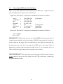
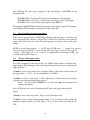
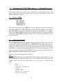
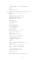
Swanson (1962) was one of the first to utilize Marshall’s analytical solutions, by applying
them to the analysis of the ‘compensation’ heat pulse method in which two temperature
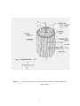
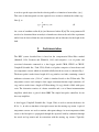
sensors are placed asymmetrically either side of a line heater source (Fig. 1). Swanson
showed that if the temperature rise following the release of a pulse of heat is measured at
distances Xu [m] upstream and Xd [m] downstream from the heater, then the heat-pulse
velocity can be calculated from
 X + Xu 
V =  d

 2 tz 
(1)
where tz [s] is the time delay for the temperatures at points Xd and Xu to become equal. In
effect, Eq. (1) implies that following the application of an instantaneous heat-pulse, the
centre of the heat-pulse is convected downstream, from the heater, to reach the point midway between the two temperature sensor after a tz. Equation (1) is particularly well suited
to data logging since it only requires electronics to detect a null temperature difference
and an accurate timer to measure tz. The tz’s are the only data that need to be recorded,
since the distances Xu and Xd remain constant. We refer to this estimate of V [m s-1] as the
‘raw’ heat -pulse velocity.
1.3
Wound Corrections to the Heat-Pulse Velocity
The calculation of V from Eq (1) is based on Marshall’s (1958) idealize d theory and
assumes the heat-pulse probes have no effect on the measured heat flow. In reality,
convection of the heat pulse is perturbed by the presence of the heater and temperature
6
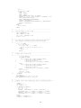
Figure 1.
Arrangement of sensors within a plant stem for the compensation heatpulse method.
7
probes, and by the disruption of xylem tissue associated with their placement. These
perturbations produce a systematic underestimation in the measured heat-pulse velocity
(Cohen et al., 1981; Green and Clothier, 1988). Consequently, the heat-pulse velocity
must be corrected for the probe-induced effects of wounding. This correction can be done
empirically (e.g. Cohen et al., 1981), or it can be based on sound physical principals,
using an equation of the form:
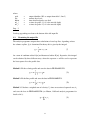
Vc = a + bV + cV 2
(2)
where Vc [m s-1] is the corrected heat-pulse velocity and V is the raw heat-pulse velocity
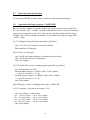
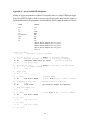
given by Eq. (1). The correction coefficients a, b, and c have been derived by Swanson
and Whitfield (1981) from numerical solutions of Marshall’s (1958) equations, for
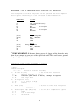
various wound sizes. The full range of correction factors are listed in Table 1. These
correction factors can also be seen in the ANALYSIS program, HPV-2000.FOR, which is
described later. The use of Eq. (2) puts the heat-pulse method on a sound theoretical
basis, and uses physical principals rather than an empirical calibration to obtain the best
estimate of the heat-pulse velocity.
Wound
a
b
c
0.0
0.000
1.000
0.000
1.6
0.393
1.356
0.036
2.0
0.807
1.203
0.058
2.4
1.184
1.072
0.087
2.8
1.524
0.964
0.124
3.2
1.826
0.879
0.169
3.6
2.090
0.818
0.221
width (mm)
Table 1. Wound corrections for Eq. (2)(From Swanson and Whitfield, 1981)
8
At this point, we note that a priori the wound size is not known, although we might
expect it to be a little larger than the size of the drill hole. This is because of additional
damage which results from mechanical disruption of vessels at the edges of the drill hole.
Anatomical investigations by Barrett et al. (1995) indicated the total wound width is
likely to extend about 0.3 mm either side of the drill hole. Thus, a wound correction of
(1.8 + 2× 0.3) mm seems appropriate for a drill hole of 1.8 mm (as used here). We have
used this wound width to successfully validate the heat-pulse method in apple, but found
a larger wound correction of some 3.2 mm was required for kiwifruit vines to bring the
heat-pulse measurement into line with actual flow rates (Green and Clothier, 1988).
Kiwifruit have very large xylem vessels and a substantial interstitial area of woody matrix
which affects the thermal homogeneity of the sapwood and, therefore, affects the
transmission and measurement of heat-pulse in kiwifruit. Our results (Green and Clothier,
1988) and the results of Barrett et al. (1995) show the importance of validating the heatpulse method in order to determine the appropriate wound factor. Such a validation is
useful, and sometimes necessary, in order to reach a good level of competence and
confidence in using the heat-pulse method.
We also issue a practical warning: if due care is not taken to align the centers of the drill
holes with the longitudinal direction of the sap flow, then the actual wound width could
well be higher than expected. In practice, we believe the 2.4 mm wound correction to be
the lower limit appropriate for probes of 1.8 mm diameter. We also stress the importance
of being careful when placing sensors in the tree stem since the calculations of total sap
flow are very sensitive to the wound factor.
A final point on the wound corrections: if the probes are left in place for an extended
period, e.g. many months, then the initial wounding may be expected to increase. This is
because of increased blockage due to tylose formation in the vessels close to the probes,
which may occur as the tree reacts to further isolate the ‘wound’. An increased wound
reaction could reduce the sensitivity of the sap flow measurements. However, we have
never experienced a significant decrease in the heat-pulse sensitivity over time, in either
9
apple or kiwifruit, and so we have been able to use the same set of probes for periods of
up to 3 months. In other species this may not be the case and then some reasoned
assessment, or independent measure of transpiration, should be made to determine just
how long the probes remain useful.
1.4
Converting Heat-Pulse Velocity to Sapflow
Once the corrected heat-pulse velocity, Vc, has been determined, the next step is to relate
it to the actual sap flow. Marshall’s (1958) analysis showed that if the sap and woody
matrix are considered to form a homogeneous medium, then the sap flux density, J [m s1
], can be calculated from
J = P ( 0.33 + M ) Vc
(3)
where P [kg m-3] is the wood density (oven dry weight of wood/green volume) and M is
the moisture content ((wet weight - oven dry weight)/oven dry weight) of sapwood. The
density and moisture content of the sapwood are both physical properties of the woody
matrix, and they can be determined easily from trunk cores. The factor 0.33 in Eq (3) is
the specific heat of dry wood, which is assumed to be constant. In our analysis, we use an
alternative expression for J, which was developed by Edwards and Warrick (1984) by
considering the sapwood to comprise 3 phases of gas, solid and liquid with appropriate
physical and thermal properties. The working equation is given by
J = ( 0.505 FM + FL ) Vc
(4)
where FM and FL are the volume fractions of wood and water, respectively. The factor
0.505 is related to the thermal properties of the woody matrix, and is assumed to be
constant within and between species.
1.5.
Measuring the Volume fractions, FM and FL
Volume fractions FM and FL implicit in Eq. (4) are determined from the Archimede’s
principle, in the following manner. Firstly, a core sample is taken and its fresh weight, MF
[kg], is determined. This weight is equal to the mass of water and the mass of dry wood,
10
since the mass of air is negligible. The core sample is then immediately submerged in a
beaker of water which has been placed on an accurate mass balance. The balance reading
will indicate an immediate increase in mass, which equals the displacement of water, DT
[kg]. The total volume, VT [m3], of the sample is then equal to ρL times DT, where the
density of water, ρL, is assumed to be 1000 kg m3. The core sample is then oven-dried to
determine the mass of dry wood, MD [kg]. The difference between the fresh weight and
the dry weight, (MF-MD) is equal to the mass of water, ML [kg], contained in the fresh core
sample. Thus, the volume fraction of water is FL = ML/(ρLVT). Similarly, the volume
fraction of wood FM = MD/(ρMVT) where the density of dry wood, ρM equals 1530 kg m3.
1.6.
Estimating Volumetric Sapflow
Equation (4) provides an estimate of the values of J at any point in the conducting
sapwood. It is widely recognized that sap flux density is not uniform throughout the
sapwood, but rather peaks at a depth of 10 - 20 mm in from the cambium. Consequently,
sampling at several depths in the sapwood is necessary to characterize the sapflow
velocity profile (Cohen et al., 1981; Edwards and Warrick, 1984; Green and Clothier,
1988). A volumetric measure of total sap flux can be obtained by the integration of these
point estimates over the sapwood conducting area. The most common approach is to fit a
least-squares polynomial to the depthwise estimates of sap flux density, and then to
integrate the fitted function over the sapwood cross section. This is the approach that we
favour. An alternative, simpler integration method, as presented by Hatton et al. (1990), is
based on a weighted average approach. According to Hatton et al. this simpler approach is
a more robust estimator of the volume flux when the velocity profiles exhibit large
curvature.
In the ANALYSIS program described later we use the most common approach to
calculate volume sap flow. Since our probes measure J at four radial depths, we fit a
second-order regression of the form
J (r ) = αr 2 + βr + γ
11
(5)
in order to get the expression for the velocity profile as a function of stem radius, r [m].
This curve is then integrated over the sapwood cross-section to calculate the volume sap
flux, Q, as
R
Q = ∫ 2πr J ( r ) dr
(6)
H
for a stem of cambium radius R [m] and heartwood radius H [m].The stem parameter H
needs to be determined from an analysis of trunk cores taken at the end of the experiment
while R can be derived from the stem circumference and an allowance for the depth of the
bark.
2.
Instrumentation
The HPV system described here is based on the ‘compensation’ Heat -Pulse method
(Marshall, 1958; Swanson and Whitfield, 1981) and comprises a set of probes and
associated electronics connected to a data logger (model CR10, CR21X or CR23X,
Campbell Scientific Inc., Utah, USA). Each set of probes comprises a linear heater and
two temperature sensors which are installed radially into the tree stem, as shown in Fig. 1.
The heater probe is made from a length of 19 swg stainless steel tube, containing a central
nichrome resistance wire (5 Ω m-1) which is insulated inside a fine Teflon tube. The
temperature sensors each comprise four copper-constantan thermo-couple junctions (42
swg) and are made from a length of Teflon tubing (18 swg) which is filled with epoxy
resin. The electronics consists of a heater controller and a set of linear instrumentation
amplifiers which have a gain of about 5000. The simple heat-pulse controllers do not
have any amplifiers.
A data logger (Campbell Scientific Inc., Logan, Utah) is used to activate the heater, for
0.5 to 1 s, in order to introduce a heat-pulse tracer into the moving sap stream. A pair of
temperature sensors are used to monitor subsequent changes in stem temperature which
occur as the heat-pulse is propagated through the sapwood, both by conduction through
the wood and sap matrix and by convection with the moving sap streams. Typically,
12
output signals from the HPV unit should lie between ± 40 mV for the 1oC difference in
temperature difference between the two sensors. The data logger is programmed to
interpret the temperature signals and to record the subsequent ‘cross-over’ times which
are used in Eq. (1) to calculate the raw heat-pulse velocity at a single point (depth) in the
conducting sapwood. A laptop PC is later used to retrieve the tz data from the logger and
to calculate total sap flow in the tree stem, as described by Eqs. (4) - (6).
3.
Connecting up the logger
and getting it going.
This section refers to installation and operation of the the HPV units. The wiring and
operation of the simple heat-pulse controller (no amplifiers) is described in Appendix B.
3.1
Assembling the necessary hardware.
The following is a list of hardware needed to run the HPV unit.
3.1.1. You will need 2 sets of:
.. heat pulse probes (white ones with grey connectors)
.. heat pulse cables (white ones with silver connectors)
and 1 set of:
.. heat pulse unit with power lead
.. suite of heat pulse programs to capture and analyze the heat-pulse data
The above items are supplied with your installation.
3.1.2. You will also need:
.. Campbell Datalogger (CR10X, CR21X or CR23X)
.. external 12V (>70 AHr) battery
.. Laptop with SC32 interface and Campbell Software (PC208W)
These items are not supplied with your installation.
13
3.2.
Connecting the HPV unit to the data logger:
There are two leads which must to be connected to the HPV unit - a signal lead and a
power lead. The pin-out of these leads is listed below.
Signal lead: This lead has 7 coloured wires which must be connected as follows:
orange
orange/white
blue
blue/white
green
green/white
white
=
=
=
=
=
=
=
1H or 3H or 5H
1L or 3L or 5L
2H or 4H or 6H
2L or 4L or 6L
AG
C1 or C2 or C3
AG or GND
(analog input)
“
“
“
(analog ground)
(control line)
(cable shield)
Power lead: This lead has 2 coloured wires which must be connected as follows:
black = GRND
red = +12V
IMPORTANT: The black and red wires go to the POWER on the heat-pulse unit. A
separate battery should be used for the logger. ALWAYS connect the red wire first, to
avoid shorting out the logger. Also, be careful that you don’t plug the wrong cable into
the heat-pulse unit, since this may short-out the HPV unit or the logger (It hasn’t
happened yet, but that’s little consol ation for when it does!!!). As a precaution, there is a
diode inside the heat-pulse unit to protect it against reverse-polarity.
VERY IMPORTANT: If the same battery powers the logger and the heat-pulse unit then
do not connect the green wire of the signal lead to AG. This would cause a ground loop
and might affect the results...
14
4. Installing the heat-pulse probes.
This section gives advice on how to install the heat-pulse probes into a plant stem. Note:
It is good practice to test the operation of the logger and the probes, and to test all the
wiring connections before inserting the probes into the plant stem. Although the HPV unit
is designed to be operated automatically, the software does allow for a manual test of the
system, as described later in the next section.
4.1. Checking if probes are OK
The pin-out for the connector on the temperature probes (the 9-pin D-plug) is:
1&6 =
2&7 =
3&8 =
4&9 =
channel 1 (outer-most sensor, closest to the cambium)
channel 2
channel 3
channel 4 (inner-most sensor, closest to the stem centre)
Each temperature sensors should be electrically isolated. A quick ‘beep-test’ of the
temperature sensors using a multi-meter should confirm each thermocouple is connected,
and isolated from the others. The temperature probes should have a resistance of about 19
ohms. The heater probe normally has a resistance of about 0.4-0.6 ohms. If the heater is
faulty then this resistance will exceed this value.
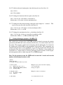
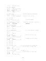
4.2. Procedure for installing probes.
4.2.1. Locate a fairly straight piece of stem, fairly free of bumps
and knots. Measure the stem circumference, C, to the nearest
mm.
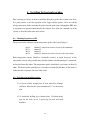
4.2.2. Attach the drilling jig as shown below. Use thick stickytape for the stem, or use a special jig for roots and small
branches.
15
this is the downstream probe (unmarked)
e.g. the highest probe in the stem or
the root probe nearest to the stem
this is the heater probe
this is the upstream probe (marked with a dot)
Sap flow
4.2.3. Carefully drill the holes using a high-speed, electric drill.
• Don’t drill too far at once (say more than 20mm) because this can
'over
-bore' the hole. Make sure the hole is about 20 mm deeper than
the longest probe.
• Remove the jig and 'plug’ the holes with Vaseline.
• Take a 'cork bore' around the two outer holes so you can measure
the bark depth, D (mm), e.g. with a set of calipers.
insert:
• Dip each probe in Vaseline, and then insert it CAREFULLY into
the appropriate hole. The probe marked with the red dot goes
closest to the heater. Insert the heater last.
• Tape the probes CAREFULLY to the tree stem, but don’t bend
them to far!!
• Check each probe to make sure its OK (see 4.1)
IF its OK THEN
• connect it to the logger.
ELSE
• get some new probes
• goto insert
ENDIF
4.3.
Testing if everything is working.
Make sure the HPV system is properly connected (see 3.2 above)
Make sure the logger is properly programmed (see 5 below)
Fire a test pulse (see 5 below)
IF it seems to be OK THEN
go for a beer
16
ELSE
swear a lot
blame someone else (but not me)
goto deep_shit
ENDIF
Note1: if you cant find deep_shit, then your not in it.
Note2: There is no deep_shit. I expect that every thing will work
Note3: Murphy’s Law suggests there will be some other problem to find.
5.
Installing the data-logger software
The following program is to be run on a Campbell data logger. The logger software is
located in one of the three sub-directories on the disk provided with the installation.
5.1.
Files in A:\LOGGER
C10-HP*.STN
C10-HP*.DLD
C10-HP*.CSI
C21-HP*.STN
C21-HP*.DLD
C21-HP*.CSI
This sub-directory contains the above CAPTURE programs designed to measure the
outputs generated by the HPV unit, and to calculate and store the tZ values associated with
each set of the probes. The program is rather basic (in keeping with our philosophy). It is
intended to be run on a Campbell logger (CR10, CR21X or CR23X). A CR10 will
measure up to three sets of probes and a CR21X will measure up to four sets of probes, a
CR23X will measure up to 6 sets of probes. The whild-card ‘*’ in the file name implies
the number of probes that will be measured.
Note: A single logger can up to 6 sets of probes. It is a simple matter to extend the total
number of probes by using a Campbell AM25T solid state multiplexer, to switch the
output from many more probes. This requires a slightly modified version of the
CAPTURE program to include use of the multiplexer and to allocate the extra channels
on the logger. If the USER wishes to consider either of these modifications then examples
of the necessary programs can be supplied, via email, at a later date. Details are in
Appendix A.
In what follows, we assume the USER is familiar with the various functions of the CR10
data logger, and the Campbell programs included with the PC208 software (GraphTerm
and EDLOG).
17
The following files have been supplied in the sub-directory A:\LOGGER of the
installation disk:
CR10-HP3.STN is the Station file required to communicate with the logger.
CR10-HP3.DLD is a file to be 'downloaded’ to the logger, via the GT program.
CR10-HP3.CSI is a file created by the program editor, EDLOG.
The program CR10-HP3.DLD should be downloaded to the logger using the GT program
(see Campbell PC208 manual for instructions on how to do this).
5.3.
Down-loading programs to the logger
There are two ways to enter the CAPTURE program into the data logger - via the key pad
or by using the PC208 software as supplied by Campbell Sci. The latter is the preferred
option since GT can also be used to download program, and retrieve data, in the usual
manner.
NOTE. to get the logger-prompt '>' via GT, enter 2718H at the '*' prompt. You can now
talk to the logger via the PC, or exit GT and talk to the logger via the keypad. Special
'modes' for the logger are *1, *5, *6, and *7, as explained below. Remember, CTRL_ gets
you back to the options menu. !!!!!
5.4.
Review of the logger modes
For a full description of the logger modes, the USER should consult a Campbell datalogger manual. The following is some basic information that may help you to interpret the
logger functions.
*1 mode is used to enter and/or alter a program (Table-1) that resides in the memory of
the logger. Enter '*1 X A' to view instruction no. x in Table 1.
*5 mode is used to set the clock. !!! Most important to do this before the heat-pulse
program is run. Expect the following responses:
Enter '*5 A YY A DOY A HRMIN A' to set the year, day
-of-year and current time
in hours and minutes.
Note: PC208 can also be used to download the PC time to the logger (the preferred
option).
*6 mode is used to view and set the 'flags’ as well as the input value
*7 mode is used to examine output memory. Enter *7 to see memory pointer to the next
location in output memory (say 740). Enter *7 X to see data stored at location X (say
740).
18
5.5.
Retrieving data from the logger
Use the program PC208 to retrieve all the ‘uncollected’ data from the data logger.
5.6.
Operation of the logger program - C10-HP3.DLD
Here we describe a number of program changes and system tests that you may want to do.
We also describe some 'normal' program behaviour that may be expected during the
course of a measurement period. Note: After you have finished playing with the logger,
ALWAYS press *0 to recompile any changes, or to continue by leaving the logger in the
'LOG1' mode.
5.6.1. To change the interval between heat pulses (alter Inst-1)
enter *1 1 A A A x A *0 where x = interval in minutes
The default time is 30 minutes
5.6.2. To fire a test heat-pulse
enter *6 A D 1 (the lights should go on, and the program will run)
enter *6 A D 6 for an early exit of program
enter *0 to continue
5.6.3. To check if the system is working properly (generally a good idea!)
fire a test heat pulse (see 5.6.2)
check the initial voltages (+/- 20 mV is OK, -9999 is stuffed)
i.e. enter *6 x A where x = 41..56
check the present voltages (+/- 100 mV is OK, -9999 is stuffed)
i.e. enter *6 x A where x = 21..36
enter *0 to continue
Note. Readings are in mV so anything in the range +/- 200 is OK.
5.6.4. To examine tz data (stored in locations 1..16)
enter *6 x A where x is the location.
loc. 1 = tz1-1 (outer) .... loc. 4 = tz1-4 (inner)
loc. 5 = tz2-1 (outer) .... loc. 8 = tz2-4 (inner)
loc. 9 = tz3-1 (outer) .... loc.12 = tz3-4 (inner)
loc. 13 = tz4-1 (outer) .... loc.16 = tz4-4 (inner)
enter *0 to continue
19
5.6.5. To find out the total running-time since the heat-pulse was fired (loc. 99)
enter *6 99 A
enter *0 to continue
5.6.6. To change the duration of the heat pulse (alter Inst-44)
enter *1 44 A A A x A *0 where x is duration in s
default value is 2.0 s (this is also the maximum time)
5.6.7. To change the delay between firing a heat pulse and testing for a 'cross
-over'. This
may be necessary for really fast flows (alter Inst-49)
enter *1 49 A A A x A *0 where x is delay in multiples of 0.1s
default value is 15 s, i.e. x=150
5.6.8. To change the maximum time for a tz calculation (alter Inst-14)
enter *1 14 A A A x A where x is max time in multiples of 0.1s
default value if 500 s, i.e. x=500, but 300s might be OK
5.7.
Listing of the logger program - C10-HP3.CSI
This section gives a listing of the CAPTURE program designed to measure the outputs
generated by the HPV unit, and to calculate and store the tz’s associated with each set of
the probes. The program is rather basic (in keeping with our philosophy). It is located in
the subdirectory A:\LOGGER on the installation disk provided. This programme was
compiled using the latest version of EDLOG. As a result, the program may not install and
run properly if the old version of EDLOG and GT is used. However, if any problems do
occur then it is a simple matter to enter the following program by hand, via the keypad,
and subsequently retrieve it back using the GT (or TERM) program.
Note: For the program to run, the USER needs to enter the *A mode and reset the
number of final output locations to 100.
;{CR10}
*Table 1 Program
01: 0.2500 Execution Interval (seconds)
1: If time is (P92)
1: 0
Minutes (Seconds --) into a
2: 30
Interval (same units as above)
3: 11
Set Flag 1 High
Flag 1 is used to activate automatic sampling
once every 30 mins.
Change as required
2: If Flag/Port (P91)
1: 15
Do if Flag 5 is High
2: 30
Then Do
Flag 5 is set when tz is calculated
3: Timer (P26)
store current time in loc (99)
20
1: 99
Loc [ _________ ]
4: Volts (SE) (P1)
1: 12
Reps
2: 14
ñ 250 mV Fast Range
3: 1
SE Channel
4: 21
Loc [ _________ ]
5: 1
Mult
6: 0
Offset
Measure current temp. signal and store in loc (21..32)
Change as required
5: Beginning of Loop (P87)
1: 0
Delay
2: 12
Loop Count
Check for cross-over times
6: IF (X<=>F) (P89)
1: 1 -- X Loc [ _________ ]
2: 1
=
3: 0
F
4: 30
Then Do
Monitor loc (21..32) to observe temperature trace
Change as required
tz’s are stored in loc (1..12)
7: IF (X<=>Y) (P88)
1: 41 -- X Loc [ _________ ]
2: 3
>=
3: 21 -- Y Loc [ _________ ]
4: 30
Then Do
test for a temperature ‘cross over’
initial temperature signal in loc (41..52)
8: Z=X (P31)
1: 99
X Loc [ _________ ]
2: 1 -- Z Loc [ _________ ]
If crossed over then
store tz in loc (1..12)
9: Z=Z+1 (P32)
1: 90
Z Loc [ _________ ]
inc a ‘tz’ counter
current temperature signal in loc (21..32)
10: End (P95)
11: End (P95)
12: End (P95)
13: IF (X<=>F) (P89)
1: 90
X Loc [ _________ ]
2: 3
>=
3: 12
F
4: 16
Set Flag 6 High
If all 12 channels have crossed over then
set Flag 6
14: IF (X<=>F) (P89)
1: 99
X Loc [ _________ ]
2: 3
>=
3: 500
F
4: 16
Set Flag 6 High
If more than 500 s have elapsed then
set flag 6
Change as required
Change as required
15: End (P95)
16: If Flag/Port (P91)
1: 16
Do if Flag 6 is High
If Flag 6 is set then
output all the data
21
2: 30
Then Do
17: Do (P86)
1: 10
Set Output Flag High
18: Sample (P70)
1: 2
Reps
2: 91
Loc [ _________ ]
Ouput the date and time
19: Sample (P70)
1: 12
Reps
2: 1
Loc [ _________ ]
Output the 12 tz values
Change as required
20: Do (P86)
1: 26
Set Flag 6 Low
21: Do (P86)
1: 25
Set Flag 5 Low
22: End (P95)
23: If Flag/Port (P91)
1: 11
Do if Flag 1 is High
2: 30
Then Do
If Flag 1 is set then
Initialise and reset arrays
24: Time (P18)
1: 2
Hours into current year (maximum 8748)
2: 8784 Mod/By
3: 91
Loc [ _________ ]
Store Day of Year in loc (91)
25: Z=X*F (P37)
1: 91
X Loc [ _________ ]
2: .04167 F
3: 91
Z Loc [ _________ ]
26: Z=INT(X) (P45)
1: 91
X Loc [ _________ ]
2: 91
Z Loc [ _________ ]
27: Z=Z+1 (P32)
1: 91
Z Loc [ _________ ]
28: Time (P18)
1: 2
Hours into current year (maximum 8748)
2: 24
Mod/By
3: 92
Loc [ _________ ]
Store time (hrmin ) in loc (92)
29: Z=X*F (P37)
1: 92
X Loc [ _________ ]
2: 100
F
3: 92
Z Loc [ _________ ]
30: Time (P18)
1: 1
Minutes into current day (maximum 1440)
22
2: 60
3: 93
Mod/By
Loc [ _________ ]
31: Z=X+Y (P33)
1: 92
X Loc [ _________ ]
2: 93
Y Loc [ _________ ]
3: 92
Z Loc [ _________ ]
32: Beginning of Loop (P87)
1: 0
Delay
2: 90
Loop Count
Reset all storage arrays
33: Z=F (P30)
1: 0
F
2: 0
Exponent of 10
3: 1 -- Z Loc [ _________ ]
34: End (P95)
35: Volts (SE) (P1)
1: 12
Reps
2: 4
ñ 250 mV Slow Range
3: 1
SE Channel
4: 41
Loc [ _________ ]
5: 1
Mult
6: 0
Offset
Measure initial temp signal and store in loc (41..52)
Change as required
36: Timer (P26)
1: 0
Loc [ _________ ]
Reset timer
Monitor loc (41..52) to observe initial temp signal
37: Do (P86)
1: 21
Set Flag 1 Low
38: Do (P86)
1: 12
Set Flag 2 High
39: End (P95)
40: If Flag/Port (P91)
1: 12
Do if Flag 2 is High
2: 30
Then Do
Flag 2 is used to initiate the heat-pulse
41: Set Port(s) (P20)
1: 0
C8..C5 = 0/0/0/0
2: 111
C4..C1 = 0/high/high/high
42: Beginning of Loop (P87)
1: 1
Delay
2: 0
Loop Count
43: Timer (P26)
1: 99
Loc [ _________ ]
44: IF (X<=>F) (P89)
1: 99
X Loc [ _________ ]
Fire a 2 s heat pulse
23
2: 3
3: 2
4: 31
>=
F
Exit Loop if True
Change as required
45: End (P95)
46: Set Port(s) (P20)
1: 0
C8..C5 = 0/0/0/0
2: 0
C4..C1 = 0/0/0/0
47: Beginning of Loop (P87)
1: 1
Delay
2: 0
Loop Count
48: Timer (P26)
1: 99
Loc [ _________ ]
49: IF (X<=>F) (P89)
1: 99
X Loc [ _________ ]
2: 3
>=
3: 15
F
4: 15
Set Flag 5 High
Wait 15 s before sampling for cross overs
Change as required
50: If Flag/Port (P91)
1: 15
Do if Flag 5 is High
2: 31
Exit Loop if True
51: End (P95)
52: Do (P86)
1: 22
Set Flag 2 Low
53: End (P95)
54: Batt Voltage (P10)
1: 98
Loc [ _________ ]
Store battery voltage in loc (98)
End Program
5.8.
Operation of the logger program - C21-HP4.DLD
Here we describe the HPV program for a CR21X logger and the normal tests that you
may want to do. We also describe some 'normal' program behaviour that may be exp
ected
during the course of a measurement period. Note: After you have finished playing with
the logger, ALWAYS press *0 to recompile any changes, or to continue by leaving the
logger in the 'LOG1' mode.
5.8.1. To change the interval between heat pulses (alter Inst-1)
enter *1 1 A A A x A *0 where x = interval in minutes
24
The default time is 30 minutes
5.8.2. To fire a test heat-pulse
enter *6 A D 1 (the lights should go on, and the program will run)
enter *6 A D 6 for an early exit of program
enter *0 to continue
5.8.3. To check if the system is working properly (generally a good idea!)
fire a test heat pulse (see 5.8.2)
check the initial voltages (+/- 20 mV is OK, -9999 is stuffed)
i.e. enter *6 x A where x = 41..56
check the present voltages (+/- 100 mV is OK, -9999 is stuffed)
i.e. enter *6 x A where x = 21..36
enter *0 to continue
Note. Readings are in mV so anything in the range +/- 200 is OK.
5.8.4. To examine tz data (stored in locations 1..16)
enter *6 x A where x is the location.
loc. 1 = tz1-1 (outer) .... loc. 4 = tz1-4 (inner)
loc. 5 = tz2-1 (outer) .... loc. 8 = tz2-4 (inner)
loc. 9 = tz3-1 (outer) .... loc.12 = tz3-4 (inner)
loc. 13 = tz4-1 (outer) .... loc.16 = tz4-4 (inner)
enter *0 to continue
5.8.5. To find out the total running-time since the heat-pulse was fired (loc. 99)
enter *6 99 A
enter *0 to continue
5.8.6. To change the duration of the heat pulse (alter Inst-48)
enter *1 48 A A A x A *0 where x is duration in s
default value is 2.0 s (this is also the maximum time)
5.8.7. To change the delay between firing a heat pulse and testing for a 'cross
-over'. This
may be necessary for really fast flows (alter Inst-56)
enter *1 56 A A A x A *0 where x is delay in multiples of 0.1s
default value is 15 s, i.e. x=150
5.8.8. To change the maximum time for a tz calculation (alter Inst-15)
25
enter *1 15 A A A x A where x is max time in multiples of 0.1s
default value if 500 s, i.e. x=500, but 300s might be OK
5.9.
Listing of the logger program - C21-HP4.CSI
This section gives a listing of the CAPTURE program designed to measure the outputs
generated by the HPV unit, and to calculate and store the tz’s associated with ea ch set of
the probes. Note: For the program to run on a CR21X, the USER needs to enter the *A
mode and reset the number of final output locations to 100. The programme is similar to
C10-HP3.CSI, except for minor changes caused by instructions P20 and P30 which are
described in the Campbell data logger manual. Locations where the USER can make
changes are written in bold type.
;{21X}
*Table 1 Program
01: 0.2000 Execution Interval (seconds)
1: 41
2: 3
3: 21
4: 30
1: If time is (P92)
1: 0
Minutes into a
2: 30
Minute Interval
3: 11
Set Flag 1 High
-- X Loc [ _________ ]
>=
-- Y Loc [ _________ ]
Then Do
8: Z=X (P31)
1: 99
X Loc [ _________ ]
2: 1 -- Z Loc [ _________ ]
2: If Flag/Port (P91)
1: 15
Do if Flag 5 is High
2: 30
Then Do
9: Z=X*F (P37)
1: 1 -- X Loc [ _________ ]
2: 0.1
F
3: 1 -- Z Loc [ _________ ]
3: Timer (P26)
1: 99
Loc [ _________ ]
10: Z=Z+1 (P32)
1: 90
Z Loc [ _________ ]
4: Volts (SE) (P1)
1: 16
Reps
2: 4
ñ 500 mV Slow Range
3: 1
SE Channel
4: 21
Loc [ _________ ]
5: 1
Mult
6: 0
Offset
11: End (P95)
12: End (P95)
13: End (P95)
14: IF (X<=>F) (P89)
1: 90
X Loc [ _________ ]
2: 3
>=
3: 16
F
4: 16
Set Flag 6 High
5: Beginning of Loop (P87)
1: 0
Delay
2: 16
Loop Count
6: IF (X<=>F) (P89)
1: 1 -- X Loc [ _________ ]
2: 1
=
3: 0
F
4: 30
Then Do
15: IF (X<=>F) (P89)
1: 99
X Loc [ _________ ]
2: 3
>=
3: 5000 F
4: 16
Set Flag 6 High
7: IF (X<=>Y) (P88)
26
16: End (P95)
3: 92
17: If Flag/Port (P91)
1: 16
Do if Flag 6 is High
2: 30
Then Do
31: Time (P18)
1: 1
Minutes into current day (max 1440)
2: 60
Mod/By
3: 93
Loc [ _________ ]
18: Do (P86)
1: 10
Set Output Flag High
Z Loc [ _________ ]
32: Z=X+Y (P33)
1: 92
X Loc [ _________ ]
2: 93
Y Loc [ _________ ]
3: 92
Z Loc [ _________ ]
19: Sample (P70)
1: 2
Reps
2: 91
Loc [ _________ ]
33: Beginning of Loop (P87)
1: 0
Delay
2: 90
Loop Count
20: Sample (P70)
1: 16
Reps
2: 1
Loc [ _________ ]
34: Z=F (P30)
1: 0
F
2: 1 -- Z Loc [ _________ ]
21: Do (P86)
1: 26
Set Flag 6 Low
22: Do (P86)
1: 25
Set Flag 5 Low
35: End (P95)
36: Volts (SE) (P1)
1: 16
Reps
2: 4
ñ 500 mV Slow Range
3: 1
SE Channel
4: 41
Loc [ _________ ]
5: 1
Mult
6: 0
Offset
23: End (P95)
24: If Flag/Port (P91)
1: 11
Do if Flag 1 is High
2: 30
Then Do
25: Time (P18)
1: 2
Hours into current year (max 8748)
2: 8784 Mod/By
3: 91
Loc [ _________ ]
37: Timer (P26)
1: 0
Loc [ _________ ]
38: Do (P86)
1: 21
Set Flag 1 Low
26: Z=X*F (P37)
1: 91
X Loc [ _________ ]
2: .04167 F
3: 91
Z Loc [ _________ ]
39: Do (P86)
1: 12
Set Flag 2 High
27: Z=INT(X) (P45)
1: 91
X Loc [ _________ ]
2: 91
Z Loc [ _________ ]
40: End (P95)
41: If Flag/Port (P91)
1: 12
Do if Flag 2 is High
2: 30
Then Do
28: Z=Z+1 (P32)
1: 91
Z Loc [ _________ ]
42: Set Port (P20)
1: 1
Set High
2: 1
Port Number
29: Time (P18)
1: 2
Hours into current year (maximum
8748)
2: 24
Mod/By
3: 92
Loc [ _________ ]
43: Set Port (P20)
1: 1
Set High
2: 2
Port Number
30: Z=X*F (P37)
1: 92
X Loc [ _________ ]
2: 100
F
44: Set Port (P20)
1: 1
Set High
27
2: 3
Port Number
45: Set Port (P20)
1: 1
Set High
2: 4
Port Number
54: Beginning of Loop (P87)
1: 1
Delay
2: 0
Loop Count
46: Beginning of Loop (P87)
1: 1
Delay
2: 0
Loop Count
55: Timer (P26)
1: 99
Loc [ _________ ]
56: IF (X<=>F) (P89)
1: 99
X Loc [ _________ ]
2: 3
>=
3: 150
F
4: 15
Set Flag 5 High
47: Timer (P26)
1: 99
Loc [ _________ ]
48: IF (X<=>F) (P89)
1: 99
X Loc [ _________ ]
2: 3
>=
3: 20
F
4: 31
Exit Loop if True
57: If Flag/Port (P91)
1: 15
Do if Flag 5 is High
2: 31
Exit Loop if True
49: End (P95)
58: End (P95)
50: Set Port (P20)
1: 0
Set Low
2: 1
Port Number
59: Do (P86)
1: 22
Set Flag 2 Low
60: End (P95)
51: Set Port (P20)
1: 0
Set Low
2: 2
Port Number
61: Batt Voltage (P10)
1: 98
Loc [ _________ ]
52: Set Port (P20)
1: 0
Set Low
2: 3
Port Number
*Table 2 Program
01: 0.0000 Execution Interval (seconds)
*Table 3 Subroutines
53: Set Port (P20)
1: 0
Set Low
2: 4
Port Number
End Program
28
6.
Running the ANALYSIS software ... (still under review)
This section describes the software used to analyze the tz data collected by the data
loggers. The analysis software is located in one of the four sub-directories on the disk
provided with the installation.
6.1.
Files in A:\FORT
HPV-2000.FOR
HPV-2000.EXE
HPSAMPLE.DAT
HPHEADER.DAT
This subdirectory contains the FORTRAN programs required to analyze the heat-pulse
data (HPV-2000.FOR and HPV-2000). This program has been compiled using DigitalVisual FORTRAN Version 5.1, and should run on any PC under Windows 3.1 or higher.
The program HPV-2000.EXE can be copied to any sub-directory on a laptop or a PC. But
in order to run HPV-2000, the program and the data (e.g. hpsample.dat) should reside in
the same directory.
6.2.
Setting up the input file
The file HPHEADER.DAT is an example of the first few lines which must be at the top
of each data file. Because HPV-2000 uses a FORMATTED-read of the input data, it is
important to include a header-file at the top of the tz data, in exactly the same format as
shown below. The header-file sets up the independent parameters involved in the sapflow
calculations, e.g. sapwood radius, heartwood radius, the volume fractions of wood and
water, etc. If you are familiar with FORTRAN then you can examine the source code
(HPV-2000.FOR) to find the formatted read statement.
The process to set up the input data is as follows:
Step - 1.
Each data file should have the following 10+2n lines at the top of the data files (see e.g.
HPHEADER.DAT as supplied on disk), where n is the number of probes being read. The
example below is for n=3 sets of probes and nsensors=4 is the no. of sensors in each
probe.
nprobes:
3
nsensors:
4
4
4
wound_width: 2.40 2.40 2.40
Swanson fac: 1
v-frac wood: 0.36
v-frac wat : 0.54
sapwood_rad: 6.21 6.00 6.00
hrtwood_rad: 0.00 0.00
29
prob_depth1:
prob_space1:
prob_depth2:
prob_space2:
prob_depth3:
prob_space3:
Tmin,Tmax :
Emax values:
0.50
1.00
0.50
1.00
0.50
1.00
185.
5.00
1.20
1.00
1.20
1.00
1.20
1.00
192.
5.00
2.20
1.00
2.20
1.00
2.20
1.00
3.50
1.00
3.50
1.00
3.50
1.00
5.00
The next example is the header-file required to analyze n=2 sets of probes:
nprobes:
2
nsensors:
4
4
wound_width: 2.40
Swanson fac: 1
v-frac wood: 0.36
v-frac wat : 0.54
sapwood_rad: 6.21
hrtwood_rad: 0.00
prob_depth1: 0.50
prob_space1: 1.00
prob_depth2: 0.50
prob_space2: 1.00
Tmin,Tmax : 185.
Emax values: 5.00
2.40
6.00
0.00
1.20
1.00
1.20
1.00
192.
5.00
2.20
1.00
2.20
1.00
3.50
1.00
3.50
1.00
In the two examples given above, the program is expecting to analyze data beginning on
day of year 185 (Tmin) through until day of year 192 (Tmax). The program will also plot
the volume flow rates for each set of probes, assuming the maximum flow, Emax, equals
5.0 L h-1. Swanson’s correction factors (Table 1) are used if the parameter equals 1 (an
integer). Otherwise, inputting a zero-value means the correction factors of Green and
Clothier (1988) will be used. For wide probe spacings we recommend the Green and
Clothier factors be used. Otherwise Swanson’s factors are used for narrow spacings.
The USER can modify the input data (e.g. to change probe spacings, probe depths,
sapwood radii, etc). But, be careful to keep them in the same 'format(a16,4f8.2)',
otherwise the program will probably generate an error.
Step - 2.
Next, add the tz data collected from the logger. This data should look something like:
103,100,1200,120.5,135.6,180.2,268.2,195.6,140.2,78.2,30.4
103,100,1215,120.5,135.6,180.2,268.2,195.6,140.2,78.2,30.4
103,100,1230,120.5,135.6,180.2,268.2,195.6,140.2,78.2,30.4
103,100,1245,120.5,135.6,180.2,268.2,195.6,140.2,78.2,30.4
Note. The output from the logger is in the following format:
opid,day,hrmin,tz1_1,tz1_2,tz1_3,tz1_4,tz2_1,tz2_2,tz2_3,tz2_4
30
where
opid
day
hrmin
tz1_*
tz2_*
=
=
=
=
=
output identifier (103 ⇒ output from table 1, line 3)
current day of year
time when heat-pulse was fired
tz times for probe 1 (*=1 is the outside depth)
tz times for probe 2 (*=1 is the outside depth)
Step - 3
Just keep appending new data to the bottom of the old input file
6.3.
Examining the output file
The analysis programme outputs three calculations of total sap flow, depending on how
the volume sap flux, Q, is determined. In theory, this is given by the integral
R
Q = ∫ 2πr J ( r ) dr
(7)
H
for a stem of cambium radius R [m] and heartwood radius H [m]. In practice, this integral
can be obtained by three different ways, where the operator <> will be used to represent
the least-squares fit to the profile data.
Method 1: Fit the velocity profile and store the data in FILENAME.VEL.
R
Q = 2π ∫ r J (r ) dr
(7a)
H
Method 2: Fit the flux profile and store the data in FILENAME.FLX.
Q = 2π
R
∫
r J (r ) dr
(7b)
H
Method 3: Calculate a weighted sum of velocity, Vi, times an associated sapwood area, Ai
and store the data in FILENAME.SUM (see Hatton, 1990 and analysis programme for
details of Ai’s).
Q = ∑ Ai Vi
i
31
(7c)
For well-behaved velocity profiles (i.e. small curvature at large radii) all three methods
yield similar results, but for profiles where the curvature near the cambium method 3 is
recommended (Hatton et al, 1990).
6.4.
Listing of the ANALYSIS program
The following is a listing of the FORTRAN program HPV-2000.FOR used to analyze the
tz-data collected by the HPV data logger. The analysis procedure follows that outlined in
the Background Section of this document. This is a fairly big program – only because it
includes routines for graphical output to the screen.
c============================================================
c ... Program HPV2000.FOR to convert tz data to correct sap
c ... velocities using numerical simulation results for a
c ... given wound width and probe spacings of (-0.5,0,1.0)
C ...........................................................
C
C ...
------ LAST modified AUG, 2000, S.R. Green -----C
c============================================================
USE DFLIB
IMPLICIT NONE
c include files for MS Fortran graphics
CHARACTER*50 CTITLE, ans
REAL*8 NXPIX, NYPIX
REAL*8 X1(101), Y1(101), X2(101), Y2(101)
REAL*8 X1MIN, X1MAX, Y1MIN, Y1MAX
INTEGER IX4, IY4, CWIN/0/
LOGICAL STATUS, END_CALC
TYPE (RCCOORD)
CURPOS
TYPE (WINDOWCONFIG) WINC
TYPE (QWINFO)
QWIN
REAL TZ(4,4), HPV(4), PD(4,4), PS(4,4)
REAL TMIN, TMAX, EMIN, F0, F1, F2, BEGYR
REAL R1P, R1M, R2M, R3M, R4M, A3, A4
INTEGER IDAY, ITOD, IJ
REAL WC1(5,7), WC2(5,7)
REAL R(4), SV(4), SF(4)
REAL SVIJ(16),T(100), Y(100)
REAL SAPFLOWV(4,100), SAPFLOWF(4,100), SAPFLOWS(4,100)
REAL SWR(4), HWR(4), WW(4), EMAX(4)
REAL VFWOOD, VFWAT, TOD
REAL A0, A1, A2, FLUXVEL, FLUXFLX, FLUXV(4), FLUXF(4)
REAL ID, MI, PI, TWOPI
REAL CHANID,DAY,HRMIN, HR, MIN
INTEGER NHPV, N, I, ICORR, IW(4), J, NCOL(4), NTC(4), NC
CHARACTER*40 FILNAM
CHARACTER*4 STR
LOGICAL SWANCOR
INTEGER*2 DUMMY2, FGD
INTEGER*4 DUMMY4, BGD
COMMON WINC
COMMON QWIN
C------------------------------------------------------------c ... Set the wound corrections of Swanson and Whitfield (1983)
C------------------------------------------------------------DATA WC1/
0, 0, 1,
0,
0.0,
*
16, 0.393,
1.356,
0.036,
0.0,
*
20, 0.807,
1.203,
0.058,
0.0,
*
24, 1.184,
1.072,
0.087,
0.0,
*
28, 1.524,
0.964,
0.124,
0.0,
32
*
*
32,
36,
1.826,
2.090,
0.879,
0.818,
0.169,
0.221,
0.0,
0.0 /
C------------------------------------------------------------c ... Set the wound corrections of Green and Clothier (1988)
C------------------------------------------------------------DATA WC2/
0, 0, 1,
0,
0.0,
*
16, -0.171,
1.299,
0.0194,
-0.000093,
*
20, -0.159,
1.318,
0.0270,
-0.000140,
*
24, -0.135,
1.326,
0.0367,
-0.000194,
*
28, -0.143,
1.306,
0.0488,
-0.000267,
*
32, -0.067,
1.355,
0.0571,
-0.000203,
*
36, -0.013,
1.379,
0.0670,
-0.000105/
PI=3.14159
TWOPI=2.*PI
C-----------------------------------------------------------c ... Set the graphics mode
C-----------------------------------------------------------CTITLE(1:40) = '
HEAT-PULSE analysis program
'
CALL GRAPHICSMODE(CTITLE)
1
CALL CLEARSCREEN($GCLEARSCREEN)
CALL SETTEXTPOSITION(5,1,CURPOS)
NXPIX = WINC.NUMXPIXELS !-20
NYPIX = WINC.NUMYPIXELS !- 100
NCOL(1)=4
NCOL(2)=10
NCOL(3)=1
NCOL(4)=15
BEGYR = -9999
C-----------------------------------------------------------C ... Open input/output files
C-----------------------------------------------------------WRITE(*,'(a\)') 'Enter the Input filename (.dat):
'
READ(*,'(A)') FILNAM
CALL NCSTRING(FILNAM,NC)
OPEN(UNIT=30, FILE=FILNAM(1:NC)//'.DAT', STATUS='UNKNOWN')
OPEN(UNIT=31, FILE=FILNAM(1:NC)//'.VEL', STATUS='UNKNOWN')
OPEN(UNIT=32, FILE=FILNAM(1:NC)//'.FLX', STATUS='UNKNOWN')
OPEN(UNIT=33, FILE=FILNAM(1:NC)//'.SUM', STATUS='UNKNOWN')
C-----------------------------------------------------------c ... Read input data
C-----------------------------------------------------------WRITE(*,*)
WRITE(*,*) 'Enter the number of heat pulse probes (1..4)'
READ(30,1099) ANS, NHPV
1099 FORMAT(A16,4I8)
WRITE(*,1099) ANS, NHPV
WRITE(*,*)
WRITE(*,*) 'Enter the number of sensors in each probe'
READ(30,1099) ANS, (NTC(J), J=1,NHPV)
WRITE(*,*) 'Enter the wound width from 1.6 to 3.6 (mm)'
READ(30,1098) ANS, (WW(I), I=1,NHPV)
1098 FORMAT(A16,4F8.2)
WRITE(*,1098) ANS, (WW(I), I=1,NHPV)
SWANCOR = .FALSE.
READ(30,1099) ANS, ICORR
IF(ICORR.GT.(0.0)) THEN
WRITE(*,*) 'Use Swansons corrections: YES'
SWANCOR=.TRUE.
ELSE
WRITE(*,*) 'Use Swansons corrections: NO'
SWANCOR=.FALSE.
ENDIF
WRITE(*,*)
12
DO 12 J=1,NHPV
IF(WW(J).EQ.(0.0)) IW(J) = 1
IF(WW(J).GE.(1.6)) IW(J) = INT((WW(J)-1.6)/0.4+2.5)
IF(IW(J).GT.7)
IW(J) = 7
CONTINUE
C------------------------------------------------------------
33
c ... vfwood = volume fraction of wood = 0.34
c ... vfwat = volume fraction of water = 0.56
C-----------------------------------------------------------WRITE(*,*) 'Enter the volume fraction of wood '
READ(30,1098) ANS,VFWOOD
WRITE(*,*) 'Enter the volume fraction of water '
READ(30,1098) ANS,VFWAT
C-----------------------------------------------------------c ... mean sap wood radius in cm
C-----------------------------------------------------------WRITE(*,*) 'Enter the sap-wood radius of each stem/root [cm] '
READ(30,1098) ANS, (SWR(J), J=1,NHPV)
WRITE(*,1098) ANS, (SWR(J), J=1,NHPV)
WRITE(*,*) 'Enter the heartwood radius of each stem/root [cm] '
READ(30,1098) ANS, (HWR(J), J=1,NHPV)
WRITE(*,1098) ANS, (HWR(J), J=1,NHPV)
WRITE(*,*)
C-----------------------------------------------------------c ... read in the probe depths
C-----------------------------------------------------------WRITE(*,*) 'Enter the thermistor depths of each probe [cm] '
DO 30 J=1,NHPV
READ(30,1098) ANS, (PD(I,J),I=1,NTC(J))
WRITE(*,1098) ANS, (PD(I,J),I=1,NTC(J))
READ(30,1098) ANS, (PS(I,J),I=1,NTC(J))
WRITE(*,1098) ANS, (PS(I,J),I=1,NTC(J))
DO 30 I=1,NTC(J)
30
PD(I,J) = ABS(SWR(J)-PD(I,J))
WRITE(*,*)
C------------------------------------------------------------c ... read plot range
C------------------------------------------------------------WRITE(*,*) 'Enter DOY range: Tmin, Tmax'
READ(30,1098) ANS, TMIN,TMAX
WRITE(*,1098) ANS, TMIN,TMAX
WRITE(*,*) 'Enter SAPFLOW range: Emin, Emax'
READ(30,1098) ANS, (EMAX(I), I=1,NHPV)
WRITE(*,1098) ANS, (EMAX(I), I=1,NHPV)
EMIN = 0.0
CALL SETTEXTPOSITION(33 ,35,CURPOS)
WRITE(*,*) '***** Click <MOUSE> to END *****'
CALL MOUSECLICK(IX4,IY4)
CALL CLEARSCREEN($GCLEARSCREEN)
STATUS = SETCOLOR(8)
STATUS = RECTANGLE($GFILLINTERIOR,0,0,NXPIX,NYPIX)
STATUS = SETCOLOR(2)
c-----------------------------------------------------------c ... main Loop
c-----------------------------------------------------------IDAY=0
100
READ(30,*,END=1000) CHANID,DAY,HRMIN,
*
((TZ(I,J),I=1,NTC(J)),J=1,NHPV)
IF(BEGYR.LT.0) THEN
TMIN = DAY
BEGYR = 9999
ENDIF
IF(HRMIN.LT.5) THEN
IDAY=IDAY+1
DO 120 J=1, NHPV
DO 110 I=1,ITOD
X1(I) = T(I)
Y1(I) = SAPFLOWV(J,I)
110
CONTINUE
X1MIN = TMIN !T(1)
X1MAX = TMIN+5. !T(ITOD)
Y1MIN = EMIN
Y1MAX = EMAX(1)
CALL NEWONEPLOT(X1,Y1,ITOD,'Day of Year', ''
&,'Water_Use_[L/h]','', X1MIN,X1MAX,Y1MIN,Y1MAX,.TRUE.,.FALSE.,8+J)
120
CONTINUE
34
ITOD = 1
IF(IDAY.GT.5) THEN
IDAY = 1
TMIN = TMIN+5
TMAX = TMAX+5
CALL SETTEXTPOSITION(33 ,35,CURPOS)
WRITE(*,*) '***** Click <MOUSE> to CONTINUE *****'
CALL MOUSECLICK(IX4,IY4)
CALL CLEARSCREEN($GCLEARSCREEN)
STATUS = SETCOLOR(8)
STATUS = RECTANGLE($GFILLINTERIOR,0,0,NXPIX,NYPIX)
STATUS = SETCOLOR(2)
ENDIF
ELSE
ITOD = ITOD+1
ENDIF
C-----------------------------------------------------------c ... convert hrmin to time of day
C-----------------------------------------------------------HR = INT(HRMIN/100)
MIN = HRMIN - 100*HR
TOD = DAY + (HR+MIN/60)/24
T(ITOD) = TOD
C-----------------------------------------------------------c ... For each set of probes find the corrected SV profile,
C ... then compute flux using three different methods
C-----------------------------------------------------------DO 300 J=1,NHPV
DO 200 I=1,NTC(J)
IF( TZ(I,J).gt.(0.0) ) THEN
HPV(I) = PS(I,J)/(2.*TZ(I,J))*3600.
ELSE
HPV(I) = 0.0
ENDIF
C-----------------------------------------------------------c ... compute the corrected SV
C-----------------------------------------------------------IJ=(J-1)*NTC(J)+I
IF(SWANCOR) THEN
SV(I) =(WC1(5,IW(j))*HPV(I)*HPV(I)*HPV(I)
*
+ WC1(4,IW(j))*HPV(I)*HPV(I)
*
+ WC1(3,IW(j))*HPV(I)
*
+ WC1(2,IW(j)))*(0.505*VFWOOD + VFWAT)
ELSE
SV(I) =(WC2(5,IW(j))*HPV(I)*HPV(I)*HPV(I)
*
+ WC2(4,IW(j))*HPV(I)*HPV(I)
*
+ WC2(3,IW(j))*HPV(I)
*
+ WC2(2,IW(j)))*(0.505*VFWOOD + VFWAT)
ENDIF
R(I) = PD(I,J)
SVIJ(IJ) = SV(I)
SF(I) = SV(I)*R(I)
200
CONTINUE
N = NTC(J)
CALL REGRESS(N, R, SV, A0, A1, A2)
CALL REGRESS(N, R, SF, F0, F1, F2)
C-----------------------------------------------------------c ... compute total flow, making sure that it remains positive !!!
C-----------------------------------------------------------FLUXV(J) = 0.0
FLUXF(J) = 0.0
ID = HWR(J)-0.01
DO WHILE(ID.LT.SWR(J))
ID = ID + 0.01
MI = ID + 0.005
FLUXVEL = TWOPI*MI*(A0 + A1*MI + A2*MI*MI)*0.01
IF(FLUXVEL.GT.(0.0)) FLUXV(J) = FLUXV(J) + FLUXVEL
FLUXFLX = TWOPI*(F0 + F1*MI + F2*MI*MI)*0.01
IF(FLUXFLX.GT.(0.0)) FLUXF(J) = FLUXF(J) + FLUXFLX
END DO
FLUXV(J) = FLUXV(J)/1000
FLUXF(J) = FLUXF(J)/1000
35
SAPFLOWV(J,ITOD) = FLUXV(J)
SAPFLOWF(J,ITOD) = FLUXF(J)
c
GOTO 299
C-----------------------------------------------------------C ... compute sum of sap velocity times relative sapwood area
C-----------------------------------------------------------R1P = SWR(J)
R1M = (R(1)+R(2))/2.
R2M = (R(2)+R(3))/2.
R3M = (R(3)+R(4))/2.
R4M = HWR(J)
A1=(R1P*R1P-R1M*R1M)*PI
A2=(R1M*R1M-R2M*R2M)*PI
A3=(R2M*R2M-R3M*R3M)*PI
A4=(R3M*R3M-R4M*R4M)*PI
SAPFLOWS(J,ITOD) = A1*SV(1)+A2*SV(2)+A3*SV(3)
SAPFLOWS(J,ITOD) = (SAPFLOWS(J,ITOD)+A4*SV(4))/1000.
299
CONTINUE
C-----------------------------------------------------------c ... print out the results
C-----------------------------------------------------------300
CONTINUE
301
CONTINUE
WRITE(31,995) T(ITOD), (SAPFLOWV(J,ITOD) , J=1,NHPV)
C
*
,(SAPFLOWV(1,ITOD)+SAPFLOWV(2,ITOD))/2.
WRITE(32,995) T(ITOD), (SAPFLOWF(J,ITOD) , J=1,NHPV)
C
*
,(SAPFLOWF(1,ITOD)+SAPFLOWF(2,ITOD))/2.
WRITE(33,995) T(ITOD), (SAPFLOWS(J,ITOD) , J=1,NHPV)
C
*
,(SAPFLOWS(1,ITOD)+SAPFLOWS(2,ITOD))/2.
GOTO 100
1000
CONTINUE
999
FORMAT(2A40)
996
FORMAT(5x,'Time [d] = ',F8.3,'
Sap flow [L/h] = ',8F8.3
*
,6X,1H.)
995
FORMAT(1X,F8.3,8F8.3)
C-----------------------------------------------------------CALL SETTEXTPOSITION(33 ,35,CURPOS)
WRITE(*,*) '***** Click <MOUSE> to END *****'
CALL MOUSECLICK(IX4,IY4)
CALL CLEARSCREEN($GCLEARSCREEN)
C-----------------------------------------------------------STOP
END
c============================================================
SUBROUTINE REGRESS(N, X, Y, A0, A1, A2)
C ... fit a parabola through the SFD data using N data points
C
of the form ... y = A0 + A1.x + A2.x^2
c============================================================
IMPLICIT NONE
REAL X(4), Y(4), A0, A1, A2
REAL SX, SY, SX2, SXY, SX2Y, SX3, SX4
REAL SSX2, D
INTEGER N, I
100
IF(N.GT.2) THEN
SX = 0
SY = 0
SX2 = 0
SXY = 0
SX3 = 0
SX2Y = 0
SX4 = 0
DO 100 I=1,N
SX = SX + X(I)
SY = SY + Y(I)
SXY = SXY + X(I)*Y(I)
SX2 = SX2 + X(I)*X(I)
SX2Y= SX2Y+ X(I)*X(I)*Y(I)
SX3 = SX3 + X(I)**3
SX4 = SX4 + X(I)**4
CONTINUE
SSX2= SX2
SX4 = SX4 - SX2*SX2/N
36
SX3 = SX3 - SX*SX2/N
SXY = SXY - SX*SY/N
SX2Y= SX2Y- SX2*SY/N
SX2 = SX2 - SX*SX/N
D
= SX2*SX4 - SX3**2
A1 = (SX4*SXY - SX3*SX2Y)/D
A2 = (SX2*SX2Y - SX3*SXY)/D
A0 = SY/N - A1*SX/N - A2*SSX2/N
ELSE
A0 = (Y(1)+Y(2))/2.
A1=0.0
A2=0.0
ENDIF
RETURN
END
!==========================================================
SUBROUTINE GRAPHICSMODE(CTITLE)
!==========================================================
USE DFLIB
IMPLICIT NONE
TYPE (WINDOWCONFIG) WINC
TYPE (QWINFO)
QW
INTEGER RETI2, CWIN/0/
LOGICAL STATUS, RESULT
CHARACTER*50 CTITLE
COMMON WINC
COMMON QW
!-----------------------------------------! ... set up the size of the frame window
!-----------------------------------------WINC.NUMXPIXELS = -1
WINC.NUMYPIXELS = -1
WINC.NUMTEXTCOLS = -1
WINC.NUMTEXTROWS = -1
WINC.NUMCOLORS
= -1
WINC.TITLE
= CTITLE
STATUS = SETWINDOWCONFIG(WINC)
IF(.NOT.STATUS) STATUS = SETWINDOWCONFIG(WINC)
STATUS = FOCUSQQ(CWIN)
!---------------------------------------! ... set the frame window to maximum
!---------------------------------------QW.TYPE = QWIN$MAX
RETI2 = SETWSIZEQQ(QWIN$FRAMEWINDOW, QW)
RETI2 = SETWSIZEQQ(CWIN, QW)
RETURN
END SUBROUTINE GRAPHICSMODE
!=========================================================
SUBROUTINE NCSTRING(STRING, NCHAR)
!=========================================================
CHARACTER*40 STRING
INTEGER NCHAR, I
I = 2
DO WHILE(STRING(I:I).NE.'')
I=I+1
END DO
NCHAR = I-1
END
!==========================================================
SUBROUTINE INLINE(NUNIT, NLINE, OP)
c ... read nlines from file nunit write to screen in OP is true
!==========================================================
IMPLICIT NONE
INTEGER I,NLINE,NUNIT
CHARACTER*80 LINE
LOGICAL OP
37
DO 10 I=1,NLINE
READ(NUNIT,99) LINE
IF(OP) WRITE(
*,99) LINE
CONTINUE
FORMAT(A75)
RETURN
END SUBROUTINE INLINE
10
99
!==========================================================
SUBROUTINE NEWONEPLOT(X1,Y1,NUM1,XTITLE, XUNIT, YTITLE, YUNIT
& ,GX1MIN, GX1MAX, GY1MIN, GY1MAX, Y1LABEL, Y2LABEL ,LCOL)
!==========================================================
USE DFLIB
IMPLICIT NONE
TYPE (WINDOWCONFIG) WINC
TYPE (QWINFO)
QW
INTEGER NUM1, NTICKX1, NTICKY1
INTEGER I, J,NXPIX, NYPIX, NC1, NC2
INTEGER IX,IY, ix4,iy4, LCOL
INTEGER STATUS
REAL*8 X1(NUM1), Y1(NUM1)
REAL*8 XX(NUM1), YY(NUM1)
REAL*8 X1MIN, X1MAX, X1RANGE, Y1MIN, Y1MAX, Y1RANGE
REAL*8 GX1MIN, GX1MAX, GY1MIN, GY1MAX
REAL*8 X1SCALE, DTICKX1, DUMMYSCALE
REAL*8 Y1SCALE, DTICKY1
REAL*8 XP,YP, NEWX1MAX
CHARACTER*40 XTITLE, XUNIT, NEWXUNIT, XTITLEUNIT
CHARACTER*40 YTITLE, YUNIT, NEWYUNIT, YTITLEUNIT, GTITLE
LOGICAL INVERT, LOGPLOT, SCALE, TALL, Y1LABEL, Y2LABEL
COMMON WINC
COMMON QW
NXPIX = WINC.NUMXPIXELS !-20
NYPIX = WINC.NUMYPIXELS !-100
X1MIN = GX1MIN
X1MAX = GX1MAX
Y1MIN = GY1MIN
Y1MAX = GY1MAX
DO 10 I=1,NUM1
XX(I) = (X1(I)-X1MIN)/(X1MAX-X1MIN)
YY(I) = (Y1(I)-Y1MIN)/(Y1MAX-Y1MIN)
CONTINUE
10
CALL AXISSET(X1MIN, X1MAX, X1SCALE, NTICKX1, DTICKX1)
! SOMETHING WRONG HERE
??
CALL AXISSET(Y1MIN, Y1MAX, Y1SCALE, NTICKY1, DTICKY1)
!
!
X1RANGE = (X1MAX-X1MIN)*X1SCALE
Y1RANGE = (Y1MAX-Y1MIN)*Y1SCALE
CALL NCSTRING(XTITLE,NC1)
CALL NCSTRING( XUNIT,NC2)
XTITLEUNIT = XTITLE(1:NC1)//XUNIT(1:NC2)
if(x1scale.gt.1.0) xtitleunit = xtitle(1:11)//']'
CALL NCSTRING(YTITLE,NC1)
CALL NCSTRING( YUNIT,NC2)
YTITLEUNIT = YTITLE(1:NC1)//YUNIT(1:NC2)
CALL SETVIEWPORT(0,0,NXPIX/1.0, NYPIX)
! FOR GRAPH1
STATUS = SETWINDOW(.TRUE.,-0.25D0,-0.50D0,1.25D0,1.15D0)
CALL TITLEAXIS(0.5D0,-0.15D0,XTITLEUNIT,1.4D0,1.4D0,NXPIX/1
,NYPIX,TALL,1)
! XAXIS TITLE
CALL PLOTXTICK(X1MIN, X1MAX, X1SCALE, NTICKX1,15, TALL
& ,1.4D0,1.4D0,NXPIX/1, NYPIX,.FALSE.)
&
IF(Y1LABEL) THEN
CALL TITLEAXIS(-0.20D0,0.5D0,YTITLEUNIT,1.4D0,1.4D0,NXPIX/1
&
,NYPIX,TALL,2)
! YAXIS TITLE
CALL PLOTYTICK(0.0D0,Y1MIN, Y1MAX, Y1SCALE, NTICKY1,15, TALL
& ,1.4D0,1.4D0,NXPIX/1, NYPIX)
38
ENDIF
IF(Y2LABEL) THEN
CALL TITLEAXIS(1.15D0,0.5D0,YTITLEUNIT,1.4D0,1.4D0,NXPIX/1
&
,NYPIX,TALL,2)
! YAXIS TITLE
CALL PLOTYTICK(1.0D0,Y1MIN, Y1MAX, Y1SCALE, NTICKY1,15, TALL
& ,1.4D0,1.4D0,NXPIX/1, NYPIX)
ENDIF
STATUS = SETCOLOR(7)
STATUS = RECTANGLE_W($GBORDER, 0.0D0,0.0D0,1.0D0,1.0D0)
CALL PLOTLINE(XX,YY,NUM1,LCOL)
RETURN
END SUBROUTINE NEWONEPLOT
!=========================================================
SUBROUTINE TITLEAXIS(WXP, WYP, AXTITLE, XW,YH
& ,NXPIX, NYPIX,TALL ,NAXIS)
!=========================================================
USE DFLIB
IMPLICIT NONE
REAL*8 WXP, WYP, DWXP, DWYP, XW, YH
CHARACTER*30 AXTITLE
INTEGER I, CHEI, CWID, NCBEG, NCEND, TLEN, NAXIS
INTEGER STATUS, NXPIX, NYPIX
LOGICAL TALL
TYPE (WXYCOORD)
WXY
TYPE (FONTINFO)
FONT
! ... set the font
STATUS = INITIALIZEFONTS()
I = SETFONT("T'COURIER NEW'H30W15")
CWID = FONT.PIXWIDTH
CHEI = FONT.PIXHEIGHT
STATUS = SETCOLOR(INT2(0))
! ... trim the string for leading blanks
NCBEG = 1
DO WHILE(AXTITLE(NCBEG:NCBEG) .EQ.'')
NCBEG = NCBEG+1
END DO
NCEND = NCBEG + LEN_TRIM(AXTITLE(NCBEG:))-1
TLEN = GETGTEXTEXTENT(AXTITLE(NCBEG:NCEND))
! ... add an offset for the text
IF(NAXIS.EQ.1) THEN
DWYP = 0.0
DWXP = -((REAL(TLEN)/2.)/REAL(NXPIX)*XW)
ELSE IF(NAXIS.EQ.2) THEN
DWYP = -((REAL(TLEN)/2.)/REAL(NYPIX)*YH)
DWXP = 0.0
ELSE
DWYP = 0.0
DWXP = -(REAL(TLEN/2.)/REAL(NXPIX)*XW)
ENDIF
CALL MOVETO_W(WXP+DWXP,WYP+DWYP,WXY)
IF(NAXIS.EQ.2) THEN
CALL SETGTEXTROTATION(900)
ELSE
CALL SETGTEXTROTATION(0)
ENDIF
CALL OUTGTEXT( AXTITLE(NCBEG:NCEND))
RETURN
END SUBROUTINE TITLEAXIS
C==========================================================
SUBROUTINE PLOTLINE(XX,YY,NUM,LCOL)
C==========================================================
USE DFLIB
IMPLICIT NONE
INTEGER I, NUM, LCOL, BGCOL
39
REAL*8 XX(NUM), YY(NUM)
LOGICAL STATUS
TYPE (WXYCOORD)
WXY
10
STATUS = SETCOLOR(LCOL)
CALL MOVETO_W(XX(1), YY(1), WXY)
DO 10 I=2,NUM
STATUS = LINETO_W(XX(I), YY(I) )
CONTINUE
RETURN
END SUBROUTINE PLOTLINE
C==========================================================
SUBROUTINE PLOTXTICK(LOWX, HIGHX, XSCALE, NTICK, NCOL,
&
TALL, XW,YH, NXPIX,NYPIX, LOGPLOT)
C==========================================================
USE DFLIB
IMPLICIT NONE
TYPE (WXYCOORD)
WXY
REAL*8 LOWX, HIGHX, XSCALE, XRANGE, XTICK, DXTICK
REAL*8 LOWY, HIGHY, YSCALE, YRANGE, YTICK, DYTICK
REAL*8 XW,YH, XLABEL
REAL*8 TICKLEN /0.025/
INTEGER I, NTICK, NCOL, NXPIX, NYPIX
LOGICAL RESULT, STATUS, TALL, LOGPLOT
! plot the xticks
STATUS = SETCOLOR(NCOL)
IF(TALL) TICKLEN = 0.015
DXTICK = 1.0D0/REAL(NTICK)
DO 10 I=0,NTICK
XTICK = REAL(I)*DXTICK
YTICK = 0.0D0
XLABEL = LOWX + XTICK*(HIGHX-LOWX)
CALL MOVETO_W(XTICK, YTICK, WXY)
RESULT = LINETO_W(XTICK, YTICK - TICKLEN)
CALL NUMAXIS(XTICK,YTICK-2.0*TICKLEN,XLABEL, XW,YH,NXPIX, NYPIX
&
,1, LOGPLOT)
!!!!! LOG PLOT ON XAXIS
XTICK = REAL(I)*DXTICK
YTICK = 1.0D0
CALL MOVETO_W(XTICK, YTICK, WXY)
RESULT = LINETO_W(XTICK, YTICK + TICKLEN)
10
CONTINUE
RETURN
END SUBROUTINE PLOTXTICK
C==========================================================
SUBROUTINE PLOTYTICK(XLOC,LOWY, HIGHY, YSCALE, NTICK, NCOL,
&
TALL, XW,YH,NXPIX, NYPIX )!,Y1TICK,Y2TICK)
C==========================================================
USE DFLIB
IMPLICIT NONE
TYPE (WXYCOORD)
WXY
REAL*8 LOWX, HIGHX, XSCALE, XRANGE, XTICK, DXTICK
REAL*8 LOWY, HIGHY, YSCALE, YRANGE, YTICK, DYTICK
REAL*8 TICKLEN /0.01/
REAL*8 XW,YH, YLABEL, XLOC
INTEGER I, NTICK, NCOL,NXPIX, NYPIX
LOGICAL RESULT, STATUS, TALL !, Y1TICK, Y2TICK
! plot the xticks
STATUS = SETCOLOR(NCOL)
IF(TALL) TICKLEN = 0.020
DYTICK = 1.0D0/REAL(NTICK)
DO 10 I=0,NTICK
YTICK = REAL(I)*DYTICK
XTICK = XLOC
YLABEL = LOWY + YTICK*(HIGHY-LOWY)
CALL MOVETO_W(XTICK, YTICK, WXY)
RESULT = LINETO_W(XTICK-TICKLEN, YTICK )
IF(XLOC.LT.0.5D0) THEN
CALL NUMAXIS(XTICK-0.05,YTICK,YLABEL, XW,YH,NXPIX
&
, NYPIX,2, .FALSE.)
!!!! NO LOG PLOT ON YAXIS
40
10
ELSE
CALL NUMAXIS(XTICK+0.1,YTICK,YLABEL, XW,YH,NXPIX
&
, NYPIX,2, .FALSE.)
!!!! NO LOG PLOT ON YAXIS
ENDIF
CONTINUE
RETURN
END SUBROUTINE PLOTYTICK
!=========================================================
SUBROUTINE NUMAXIS(WXP,WYP,VALUE,XW,YH,NXPIX,NYPIX,NAXIS, LOGPLOT)
! THE MAJOR TICKS
!=========================================================
USE DFLIB
IMPLICIT NONE
REAL*8 WXP, DWXP, WYP, DWYP, VALUE, XW,YH
INTEGER NXPIX, NYPIX, CHEI, CWID
INTEGER I, STATUS, NPOINTS/1/, NAXIS, TLEN
INTEGER NCBEG, NCEND, NC1,NC2,NC3
CHARACTER*16 TEMPSTR, FMS, LOGSTR
LOGICAL LOGPLOT
TYPE
TYPE
TYPE
TYPE
(XYCOORD) XY
(WXYCOORD) WXY
(WINDOWCONFIG) WINC
(FONTINFO) FONT
COMMON WINC
! ... get the font information
STATUS = INITIALIZEFONTS()
I = SETFONT("T'COURIER NEW'H20W10")
I = GETFONTINFO(FONT)
CWID = FONT.PIXWIDTH
CHEI = FONT.PIXHEIGHT
! ... get the tick value
WRITE(FMS,'(A5,I2,A1)') '(F10.',NPOINTS,')'
WRITE(TEMPSTR,FMS) VALUE
! ... trim the string for leading blanks
NCBEG = 1
DO WHILE(TEMPSTR(NCBEG:NCBEG) .EQ.'')
NCBEG = NCBEG+1
END DO
NCEND = NCBEG + LEN_TRIM(TEMPSTR(NCBEG:))-1
! ... add in the exponent for a log scale
IF(LOGPLOT) THEN
LOGSTR = '1E'//TEMPSTR(NCBEG:NCEND)
CALL NCSTRING(LOGSTR,NC1)
TEMPSTR(1:NC1) = LOGSTR(1:NC1)
NCBEG = 1
NCEND = NC1
ENDIF
TLEN = GETGTEXTEXTENT(TEMPSTR(NCBEG:NCEND))
! ... add an offset for the text (to centre it on the ticks)
IF(NAXIS.EQ.1) THEN
DWYP = 0.0
DWXP = -((REAL(TLEN)/2.)/REAL(NXPIX)*XW)
ELSE
DWYP = ((REAL(CHEI)/2.)/REAL(NYPIX)*YH)
DWXP = -((REAL(TLEN)
)/REAL(NXPIX)*XW)
ENDIF
CALL MOVETO_W(WXP+DWXP,WYP+DWYP,WXY)
CALL SETGTEXTROTATION(0)
CALL OUTGTEXT( TEMPSTR(NCBEG:NCEND))
RETURN
END SUBROUTINE NUMAXIS
C==========================================================
SUBROUTINE AXISSET(LOW, HIGH, RSCALE, NTICKS, DTICKS)
41
C==========================================================
IMPLICIT NONE
REAL*8 HIGH, LOW, RANGE, DLHI, DLLO, DTICKS
REAL*8 RPOW, RSCALE, RMAG, TEMP, TINY/1E-20/
INTEGER NTICKS, HELPSCALE
! ... find the range and magnitude and rescale if necessary
RPOW = 0.0D0
RANGE = HIGH - LOW
IF(LOW .EQ.0.0D0) LOW = TINY
IF(HIGH.EQ.0.0D0) HIGH = 2.0d0*LOW
IF(RANGE.EQ. 0.0D0) THEN
! THE LINE IS VERTICAL
HIGH = HIGH + 0.5
LOW = LOW - 0.5
ENDIF
DLHI = DLOG10(ABS(HIGH))
DLLO = DLOG10(ABS(LOW))
DO WHILE(DLHI.LT.0.0D0 .AND. DLLO.LT.0.0D0)
DLHI = DLHI + 3.0D0
DLLO = DLLO + 3.0D0
RPOW = RPOW + 3.0D0
END DO
HIGH = HIGH*10**RPOW
LOW = LOW*10**RPOW
RSCALE = 10**-RPOW
RANGE = HIGH-LOW
RMAG = 10**INT(DLOG10(RANGE)) ! 10S, 100S, 1000S FOR EG.
!
... determine the lhs axis value
TEMP = LOW/RMAG
! CALCULATE LOW (FOR AXIS)
LOW
= INT(TEMP)
IF(ABS(TEMP-LOW).GE.1.0E-12 .AND. TEMP.LT.0) THEN
LOW = LOW - 1
ENDIF
LOW = LOW*RMAG
! ... determine the rhs axis value
TEMP = HIGH/RMAG
! CALCULATE HIGH (FOR AXIS)
HIGH = INT(TEMP)
IF(ABS(TEMP-HIGH).GE.1E-12 .AND. TEMP.GT.0) THEN
HIGH = HIGH + 1
ENDIF
HIGH = HIGH*RMAG
! ... determine the number of axis ticks
HELPSCALE = (HIGH-LOW)/RMAG
IF(HELPSCALE.GT.5) THEN
NTICKS = 5 !HELPSCALE
ELSE
SELECT CASE (HELPSCALE)
CASE(5)
NTICKS = 5
CASE(4)
NTICKS = 4
CASE(3)
NTICKS = 3
CASE(2)
NTICKS = 4
CASE(1)
NTICKS = 5
END SELECT
ENDIF
DTICKS = (HIGH-LOW)/NTICKS
RANGE = HIGH-LOW
IF(RANGE.GE.1000) THEN
HIGH = HIGH*1.0D-3
LOW = LOW*1.0D-3
RSCALE = RSCALE*1.0D3
ENDIF
END SUBROUTINE AXISSET
!==========================================================
SUBROUTINE RANGESET(X, NX, XMIN, XMAX)
!==========================================================
IMPLICIT NONE
42
10
INTEGER I, NX
REAL*8 X(NX), XMIN, XMAX
XMIN = 1.0D10
XMAX = -1.0D10
DO 10 I=1,NX
IF(X(I).LE.XMIN) XMIN = X(I)
IF(X(I).GE.XMAX) XMAX = X(I)
CONTINUE
RETURN
END SUBROUTINE RANGESET
!==========================================================
SUBROUTINE MOUSECLICK(X,Y)
!==========================================================
USE DFLIB
IMPLICIT NONE
INTEGER*4 MOUSEEVENT, KEYSTATE, X, Y, RESULT
MOUSEEVENT = MOUSE$RBUTTONDOWN .OR. MOUSE$LBUTTONDOWN
RESULT = WAITONMOUSEEVENT(MOUSEEVENT, KEYSTATE, X, Y)
!
WRITE(5,*) 'MOUSE AT ', X, Y
RETURN
END SUBROUTINE MOUSECLICK
!==========================================================
SUBROUTINE MOUSETOEXIT(UNIT,MOUSEEVENT,KEYSTATE
& ,MOUSEXPOS,MOUSEYPOS)
!==========================================================
USE DFLIB
INTEGER UNIT,MOUSEEVENT, KEYSTATE,MOUSEXPOS, MOUSEYPOS
LOGICAL MOUSEEXIT
COMMON /MOUSE/ MOUSEEXIT
MOUSEEXIT = .TRUE.
! ONLY EXECUTED IF MOUSE LBUTTON IS PRESSED
RETURN
END SUBROUTINE MOUSETOEXIT
43
7.
References
Barrett, D.J., Hatton, T.J., Ash, J.E., and Ball, M.C., 1995. Evaluation of the heat-pulse
velocity technique for measurement of sap flow in rainforest and eucalypt forest
species of south-eastern Australia. Plant Cell Environ., 18, 463-469.
Cohen, Y., Fuchs, M., and Green, G.C., 1981. Inprovement of the heat-pulse method for
determining sap flow in trees. Plant Cell Environ, 4, 391-397.
Dye, P.J., Olbrich, B.W., and Poulter, A.G., 1991. The influence of growth rings in Pinus
patula on heat-pulse velocity and sap flow measurement. J. Exp. Bot., 42, 867870.
Edwards, W.R.N., and Warrick, N.W.M., 1984. Transpiration from a kiwifruit vine as
estimated by the heat-pulse technique and the Penman-Monteith equation. N. Z. J.
Agric. Res., 27, 537-543.
Green, S.R., and Clothier, B.E., 1988. Water use of kiwifruit vines and apple trees by the
heat-pulse technique. J. Exp. Bot., 39, 115-123.
Hatton, T.J., Catchpole, E.A., and Vertessy, R.A., 1990. Integration of sapflow velocity to
estimate plant water use. Tree Physiol., 6, 201-209.
Huber, B., 1932. Beobachtung und Messung pflanzicher Saftstrome. Ber. deutsch. Bot.
Ges., 50, 89-109.
Huber, B., and Schmidt, E., 1937. Eine Kompensationsmethode zur thermoelektrischen
Messung langsamer Saftstrome. Ber. deutch. Bot. Ges, 55, 514-529.
Marshall, D.C., 1958. Measurement of sap flow in conifers by heat transport. Plant
Physiol., 33, 385-396.
Swanson, R.H., and Whitfield, D.W.A., 1981. A numerical analysis of heat-pulse velocity
theory and practice. J. Exp. Bot., 32, 221-239.
44
Appendix A – use of an AM25T multiplexer:
Listing of logger programme to connect 3 heat-pulse units to a single CR10 data logger.
Note: One AM25T could be used to measure up to 6 heat-pulse units, but this requires a
small modification to the programme described below. Please email the author for details.
CR10:
AM25T
+12
G
C3
C2
no connection
AG
1H
1L
+12
G
CLK
RES
EX
AG
HI
LO
(1H, 1L, 2H, 2L)
(3H, 3L, 4H, 4L)
(5H, 5L, 6H, 6L)
(7H, 7L, 8H, 8L)
and so on ...
Output from box-1, probe 1
Output from box-1, probe 2
Output from box-2, probe 1
Output from box-2, probe 2
*Table 1 Program
01: 0.25
Execution Interval (seconds)
1:
1:
2:
3:
If time is (P92)
; Flag 1 is automatic sampling
0000
Minutes (Seconds --) into a ; once every 30 minutes
30
Interval (same units as above)
;Change as required
11
Set Flag 1 High
2: If Flag/Port (P91)
; Flag 5 is set when tz is calculated
1: 15
Do if Flag 5 is High
2: 30
Then Do
3: Timer (P26)
1: 99
Loc [ _________ ]
4: Do (P86)
1: 42
Set Port 2 High
5: Beginning of Loop (P87)
1: 0000
Delay
2: 12
Loop Count
; Activate AM25T
; Connect Port 2 (C2) to Reset on AM25T
; Measure inputs on 2*N boxes
; (2* N boxes) Change as required
6: Step Loop Index (P90)
1: 2
Step
7: Do (P86)
1: 43
Set Port 3 High
; Connect Port 3 (C3) to Clock on AM25T
8: Do (P86)
1: 53
Set Port 3 Low
9: Do (P86)
1: 43
Set Port 3 High
10:
Do (P86)
45
1: 53
11:
1:
2:
3:
4:
5:
6:
Set Port 3 Low
Volt (SE) (P1)
2
Reps
15
2500 mV Fast Range
1
SE Channel
31
-- Loc [ _________ ]
1.0
Mult
0.0
Offset
12: Z=X-Y (P35)
1: 31
-- X Loc [ _________ ]
2: 61
-- Y Loc [ _________ ]
3: 31
-- Z Loc [ _________ ]
13:
Calculate temperature difference
and store in loc (31..54)
End (P95)
14: Do (P86)
1: 52
Set Port 2 Low
15: Beginning of Loop (P87)
1: 0
Delay
2: 24
Loop Count
16:
1:
2:
3:
4:
If (X<=>F) (P89)
1
-- X Loc [ _________ ]
1
=
0.0
F
30
Then Do
17:
1:
2:
3:
4:
If (X<=>F) (P89)
31
-- X Loc [ _________ ]
4
<
0.0
F
30
Then Do
De-activate AM25T
; Check each input for a cross-over
8*N boxes
If a cross-over has occurred
18: Z=X (P31)
1: 99
X Loc [ _________ ]
2: 1
-- Z Loc [ _________ ]
Store tz in loc (1..24)
19: Z=Z+1 (P32)
1: 90
Z Loc [ _________ ]
Increment the ‘tz’ counter
20:
End (P95)
21:
End (P95)
22:
End (P95)
23:
1:
2:
3:
4:
If (X<=>F) (P89)
; If all 24 channels have crossed over
90
X Loc [ _________ ] ; then set flag 6 (to exit loop)
3
>=
24
F
16
Set Flag 6 High
24:
1:
2:
3:
4:
If (X<=>F) (P89)
; if time > 300 s
99
X Loc [ _________ ] ; then set flag 6 (to exit loop)
3
>=
300
F
16
Set Flag 6 High
46
25:
End (P95)
26: If Flag/Port (P91)
; Flag 6 is used to generate output
1: 16
Do if Flag 6 is High
2: 30
Then Do
27: Do (P86)
1: 10
Set Output Flag High
28: Sample (P70)
1: 2
Reps
2: 91
Loc [ _________ ]
Output the date and time
29: Sample (P70)
1: 24
Reps
2: 1
Loc [ _________ ]
Output the 24 tz values
change as required
30: Do (P86)
1: 26
Set Flag 6 Low
31: Do (P86)
1: 25
Set Flag 5 Low
32:
End (P95)
33: If Flag/Port (P91)
; Flag 1 begins the heat-pulse routine
1: 11
Do if Flag 1 is High
2: 30
Then Do
34: Time (P18)
1: 2
Hours into current year (maximum 8784)
2: 8784
Mod/By
3: 91
Loc [ _________ ]
35: Z=X*F (P37)
1: 91
X Loc [ _________ ]
2: .04167
F
3: 91
Z Loc [ _________ ]
36: Z=INT(X) (P45)
1: 91
X Loc [ _________ ]
2: 91
Z Loc [ _________ ]
37: Z=Z+1 (P32)
; Store the current day number (loc 91)
1: 91
Z Loc [ _________ ]
38: Time (P18)
1: 2
Hours into current year (maximum 8784)
2: 24
Mod/By
3: 92
Loc [ _________ ]
39: Z=X*F (P37)
1: 92
X Loc [ _________ ]
2: 100
F
3: 92
Z Loc [ _________ ]
40: Time (P18)
1: 1
Minutes into current day (maximum 1440)
2: 60
Mod/By
3: 93
Loc [ _________ ]
47
41: Z=X+Y (P33)
; Store the time (hrmin)
1: 92
X Loc [ _________ ]
2: 93
Y Loc [ _________ ]
3: 92
Z Loc [ _________ ]
(loc 92)
42: Beginning of Loop (P87)
1: 0
Delay
2: 90
Loop Count
43: Z=F (P30)
; Reset all storage arrays
1: 0
F
2: 0
Exponent of 10
3: 1
-- Z Loc [ _________ ]
44:
End (P95)
45: Do (P86)
1: 42
Set Port 2 High
; measure initial voltage using AM25T
; Port 2 is connected reset of AM25T
46: Beginning of Loop (P87)
1: 0
Delay
2: 12
Loop Count
; for 4* N boxes
47: Step Loop Index (P90)
1: 2
Step
48: Do (P86)
1: 43
Set Port 3 High
; Port 3 (C3) connects to clock of AM25T
49: Do (P86)
1: 53
Set Port 3 Low
50: Do (P86)
1: 43
Set Port 3 High
51: Do (P86)
1: 53
Set Port 3 Low
52:
1:
2:
3:
4:
5:
6:
53:
Volt (SE) (P1)
; Store initial voltage in Loc (61..84)
2
Reps
15
2500 mV Fast Range
1
SE Channel
61
-- Loc [ _________ ]
1.0
Mult
0.0
Offset
End (P95)
54: Do (P86)
1: 52
Set Port 2 Low
55: Timer (P26)
1: 0
Reset Timer
56: Do (P86)
1: 21
Set Flag 1 Low
57: Do (P86)
1: 12
Set Flag 2 High
58:
End (P95)
48
59: If Flag/Port (P91)
1: 12
Do if Flag 2 is High
2: 30
Then Do
60: Set Port(s) (P20)
; Port 1 (C1) is the heater control line
1: 0
C8..C5 = low/low/low/low
2: 1
C4..C1 = low/low/low/high
61: Beginning of Loop (P87)
1: 1
Delay
2: 0
Loop Count
62: Timer (P26)
1: 99
Loc [ _________ ]
63:
1:
2:
3:
4:
64:
If (X<=>F) (P89)
; Fire the heater for 1 s
99
X Loc [ _________ ]
3
>=
1
F
Change as required
31
Exit Loop if True
End (P95)
65: Set Port(s) (P20)
1: 0
C8..C5 = low/low/low/low
2: 0
C4..C1 = low/low/low/low
66: Beginning of Loop (P87)
1: 1
Delay
2: 0
Loop Count
67: Timer (P26)
1: 99
Loc [ _________ ]
68:
1:
2:
3:
4:
If (X<=>F) (P89)
; Wait 15 s for heat-pulse to arrive
99
X Loc [ _________ ]
3
>=
15
F
; Change as required
15
Set Flag 5 High
69: If Flag/Port (P91)
1: 15
Do if Flag 5 is High
2: 31
Exit Loop if True
70:
End (P95)
71: Do (P86)
1: 22
Set Flag 2 Low
72:
End (P95)
73: Batt Voltage (P10)
; Store battery voltage in Loc 98
1: 98
Loc [ _________ ]
49
Appendix B – use of simple heat-pulse controller (no amplifiers)
The heat-pulse controller and probes can be operated with most Campbell
data loggers. The wiring is to be connected as described below:
CR10/21X/23
Controller
+12
G
C1
AG
C2
AG
Grey (external 12V battery)
Grey/Black
Blue
of controller #1
Blue/white
“
Blue
of controller #2
Blue/white
“
(1H, 1L)
(2H, 2L)
AG
AG
Probe 1
Orange, Orange/white
Blue,
Blue/white
Green1
Shield
(3H, 3L)
(4H, 4L)
AG
AG
Probe 2
Orange, Orange/white
Blue,
Blue/white
Green1
Shield
1
VERY IMPORTANT: If the same battery powers the logger and the heat-pulse unit
then do not connect the green wire of the signal lead to AG. This would cause a ground
loop and might affect the results...
Listing of a CR10 logger programme to connect
;{CR10}
*Table 1 Program
01: 0.2500
Execution Interval (seconds)
1:
1:
2:
3:
If time is (P92)
! set for 15 min intervals
0
Minutes (Seconds --) into a
15
Interval (same units as above) ! change as required
11
Set Flag 1 High
2: If Flag/Port (P91)
1: 15
Do if Flag 5 is High
2: 30
Then Do
3: Timer (P26)
1: 99
Loc [ _________ ]
! stores the time since heat-pulse
4:
1:
2:
3:
! loc 21..28 = temperature signals
Thermocouple Temp (SE) (P13)
8
Reps
1
2.5 mV Slow Range
1
SE Channel
50
4:
5:
6:
7:
8:
1
100
21
1
0
Type T (Copper-Constantan)
Ref Temp (Deg. C) Loc [ _________ ]
Loc [ _________ ]
Mult
Offset
5: Beginning of Loop (P87)
1: 0
Delay
2: 8
Loop Count
6:
1:
2:
3:
4:
If (X<=>F) (P89)
! loc 1..8 = Tz cross-over times
1
-- X Loc [ _________ ]
1
=
0
F
30
Then Do
7:
1:
2:
3:
4:
If (X<=>Y) (P88)
41
-- X Loc [ _________ ] ! loc 41..48 = original temperature
3
>=
21
-- Y Loc [ _________ ] ! loc 21..28 = temperatures now
30
Then Do
8: Z=X (P31)
1: 99
X Loc [ _________ ]
2: 1
-- Z Loc [ _________ ]
! loc 1..8 = final Tz time
9: Z=Z+1 (P32)
1: 90
Z Loc [ _________ ]
10:
End (P95)
11:
End (P95)
12:
End (P95)
13:
1:
2:
3:
4:
If (X<=>F) (P89)
90
X Loc [ _________ ]
3
>=
8
F
16
Set Flag 6 High
14:
1:
2:
3:
4:
If (X<=>F) (P89)
99
X Loc [ _________ ]
3
>=
500
F
16
Set Flag 6 High
15:
! loc 90 = number of Tz recorded
! time (s) for last measurement
End (P95)
16: If Flag/Port (P91)
1: 16
Do if Flag 6 is High
2: 30
Then Do
17: Do (P86)
1: 10
Set Output Flag High
18: Sample (P70)
! output the
1: 2
Reps
2: 91
Loc [ _________ ]
51
day and decimal hour
19: Sample (P70)
! output the cross-over times
1: 8
Reps
2: 1
Loc [ _________ ]
20: Do (P86)
1: 26
Set Flag 6 Low
21: Do (P86)
1: 25
Set Flag 5 Low
22:
End (P95)
23: If Flag/Port (P91)
1: 11
Do if Flag 1 is High
2: 30
Then Do
24: Time (P18)
1: 2
Hours into current year (maximum 8784)
2: 8784
Mod/By
3: 91
Loc [ _________ ]
! store day of year
25: Z=X*F (P37)
1: 91
X Loc [ _________ ]
2: .04167
F
3: 91
Z Loc [ _________ ]
26: Z=INT(X) (P45)
1: 91
X Loc [ _________ ]
2: 91
Z Loc [ _________ ]
27: Z=Z+1 (P32)
1: 91
Z Loc [ _________ ]
28: Time (P18)
1: 2
Hours into current year (maximum 8784)
2: 24
Mod/By
3: 92
Loc [ _________ ]
29: Z=X*F (P37)
1: 92
X Loc [ _________ ]
2: 100
F
3: 92
Z Loc [ _________ ]
! store the hour
30: Time (P18)
1: 1
Minutes into current day (maximum 1440)
2: 60
Mod/By
3: 93
Loc [ _________ ]
31: Z=X+Y (P33)
! store the decimal hour
1: 92
X Loc [ _________ ]
2: 93
Y Loc [ _________ ]
3: 92
Z Loc [ _________ ]
32: Beginning of Loop (P87)
1: 0
Delay
2: 90
Loop Count
33: Z=F (P30)
! reset all storage
1: 0
F
2: 0
Exponent of 10
3: 1
-- Z Loc [ _________ ]
52
34:
35:
1:
2:
3:
4:
5:
6:
7:
8:
End (P95)
Thermocouple Temp (SE) (P13)
! measure initial temp difference
8
Reps
1
2.5 mV Slow Range
1
SE Channel
1
Type T (Copper-Constantan)
100
Ref Temp (Deg. C) Loc [ _________ ]
41
Loc [ _________ ] ! loc 41..48 = initial temp difference
1
Mult
0
Offset
36: Timer (P26)
1: 0
Reset Timer
37: Do (P86)
1: 21
Set Flag 1 Low
38: Do (P86)
1: 12
Set Flag 2 High
39:
End (P95)
40: If Flag/Port (P91)
1: 12
Do if Flag 2 is High
2: 30
Then Do
! fire the heat pulse
41: Set Port(s) (P20)
1: 0
C8..C5 = low/low/low/low
2: 11
C4..C1 = low/low/high/high
42: Beginning of Loop (P87)
1: 1
Delay
2: 0
Loop Count
43: Timer (P26)
1: 99
Loc [ _________ ]
44:
1:
2:
3:
4:
45:
If (X<=>F) (P89)
! fire heater for just 0.75 s
99
X Loc [ _________ ]
3
>=
.75
F
! change as required
31
Exit Loop if True
End (P95)
46: Set Port(s) (P20)
1: 0
C8..C5 = low/low/low/low
2: 0
C4..C1 = low/low/low/low
47: Beginning of Loop (P87)
1: 1
Delay
2: 0
Loop Count
48: Timer (P26)
1: 99
Loc [ _________ ]
53
49:
1:
2:
3:
4:
If (X<=>F) (P89)
! wait 10 s before making a Tz measure
99
X Loc [ _________ ]
3
>=
10
F
! change as required
15
Set Flag 5 High
50: If Flag/Port (P91)
1: 15
Do if Flag 5 is High
2: 31
Exit Loop if True
51:
End (P95)
52: Do (P86)
1: 22
Set Flag 2 Low
53:
End (P95)
54: Batt Voltage (P10)
! store battery voltage in loc 98
1: 98
Loc [ _________ ]
*Table 2 Program
01: 0.0000
Execution Interval (seconds)
*Table 3 Subroutines
End Program
*Table 2 Program
02: 0.0000 Execution Interval (seconds)
*Table 3 Subroutines
End Program
54