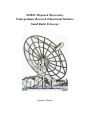
Download Code Alarm SRT 1600 Operator`s manual

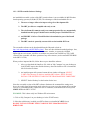
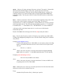
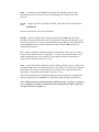
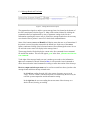
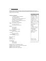
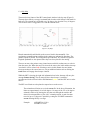
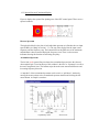
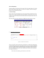
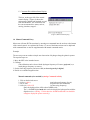
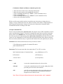
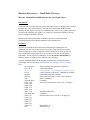
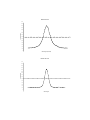
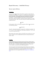
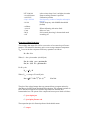
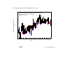
NEROC Haystack Observatory
Undergraduate Research Educational Initiative
Small Radio Telescope
Operator's Manual
Abstract
The Haystack Observatory Small Radio Telescope was developed as an educational tool to teach
concepts of radio astronomy, mechanical and electrical engineering and research methods. The
two-axis motorized mount allows the telescope to point from horizon to zenith with an azimuth
capability of nearly 360 degrees. All sky coverage is achieved through drift-scan methods. The kit
includes antenna dish, motorized two-axis mount, receiver feed, receiver electronics and JAVAbased control software. This manual is intended as a guide for the student and instructor in the
operation and data collecting of the telescope.
Further information regarding observing projects and mechanical specifications can be found on
Haystack Observatory website at http://fourier.haystack.mit.edu/SRT.
SRT Control Software, explains how to operate the telescope and how to read the main control
panel. Also included is a discussion about data reduction methods.
SRT Control Software
Table of Contents
1. Software
1.1 Overview of Capabilities
1.2 Getting Started
1.2.1 Original Full Software installation
1.2.2 Executable Software Installation
1.3 SRT Control Panel
1.3.1
1.3.2
1.3.3
1.3.4
1.3.5
1.3.6
1.3.7
Command Toolbar
Message board and Text Input
Information Sidebar
Sky Map
Spectral-line/Continuum Display
Total-Power Chart Recorder
Antenna Drive/Motion Status Display
1.4 Manual Command Entry
1.5 Input Command Files
1.6 Output Data Files
1.1 Overview of Capabilities
The SRT is capable of spectral line (1420 MHz hydrogen) and continuum observations using
source tracking, 25-point maps and drift-scans.
Aperture
LO Frequency Range
LO Tuning Step
Preamp Frequency Range
System Temperature
Pointing Accuracy
Travel Limits (degrees)
2.1
Meters
1370 - 1800
MHz
40
kHz
1400 - 1440
MHz
150
K
1
Degree
~360 Azimuth/~0-90 Elevation
See added capabilities of the digital receiver at http://web.haystack.mit.edu/SRT/receiver_1.html
1.2.1 Getting Started
The SRT control software is a JAVA-based program designed to be portable to most computer
operating-system platforms. The main telescope control interface is an active window with which
the user can enable the telescope functions either by a simple mouse click or by a combination of
mouse clicks and text entry. Users can also construct command files (form filename.cmd) which
will take data and calibrate the SRT automatically.
The control window can be seen in Figure-1. For the purposes of this tutorial, the explanation of
the control screen will be covered in seven separate sections in section 1.3.
The Java software consists of fourteen .java files.
geom.java
srt.java
global.java
checkey.java
plots.java
disp.java
cat.java
procs.java
time.java
sport.java
map.java
outfile.java
velspec.java
hdisp.java
Also needed are dynamically linked library files (.dll) which are imported when the .java files are
complied.
The user will need to import a Java Standard Edition (SDK) as well as the javacomm20-win32.zip (windows OS) for the serial port communication API. Note: Previous editions were titled
Java Development Kit (JDK)
Instructions for setting the CLASSPATH for Windows-NT and XP can be found on the Haystack
Web site at http://web.haystack.mit.edu/SRT/winNTdl.html . When you have installed your Java
Standard Edition and downloaded the SRT java files,
The syntax for compiling the SRT JAVA code is:
javac *.java
When you have compiled the code there are six run modes available to run the SRT software;
Run the SRT
Simulate SRT
Simulate Antenna
Simulate Radio
Simulate (speed time x 10)
Simulate (with 1 hour advance)
java srt 0
java srt 1 1
java srt 0 1
java srt 1
java srt 1 10
java srt 1 -1
The SRT window will open, ready for command input. Go to section 1.3 for the operational
details of the command console.
SRT users need to access an ASCII file labeled srt.cat. This file contains the user source list, the
telescope station latitude and longitude, telescope azimuth and elevation limits, in addition to
other optional information if defaults are not acceptable
An example file is listed on the next page. The file in its current configuration will allow for
commands to be properly sent to either of the three mounts currently in use or under development
for the SRT
SRT.CAT file
* sample srt.cat file
SIMULATE RECEIVER
SIMULATE ANTENNA 10
* first word is key word
* STATION: latitude longitude west in degrees
* SAT: satellite ID then longitude west
* SOU: source ra, dec, name, epoch
STATION 42.5 71.5 Haystack
* source coords epoch 1950 unless specified
SOU 05 31 30 21 58 00 Crab
SOU 23 21 12 58 44 00 Cass
SOU 00 00 00 00 00 00 Sun
SOU 17 42 54 -28 50 00 SgrA
SOU 06 29 12 04 57 00 Rosett
SOU 20 27 00 41 00 00 CygEMN
SOU 00 00 00 00 00 00 Moon
SOU 05 40 00 29 00 00 G180
SOU 12 48 00 28 00 00 GNpole
SOU 00 39 00 40 30 00 Androm
GALACTIC 10 1 RC_CLOUD
GALACTIC 229 26 test
* AZLIMITS 92.0 265.0 /* mid az range is south */
AZLIMITS 20.0 359.0
* ELLIMITS 5.0 175.0 /* elevation limit south - north */
* ELLIMITS 10.0 175.0
ELLIMITS 2.0 90.0
ALFASPID 1.0 1.0
* CASSIMOUNT 14.25 16.5 2.0 110.0 30.0
* CASSIMOUNT
COMM 1
/* COM 1 */
CALCONS 1.0
/* gain correction constant to put power in units of K */
BEAMWIDTH 7.0
/* 3 dB antenna beamwidth in degrees - used to set offsets for
scans */
MANCAL 1
/* 0 or absence indicates automated cal vane */
NOISECAL 200.0
/* initial value for noise diode calibration */
DIGITAL
/* needed for digital receiver */
TOLERANCE 1
/* optional max error in counts */
* COUNTPERSTEP 50 /* optional stepped antenna motion */
* RECORDFORM TAB VLSR /* optional tabs between fields and VLSR in output */
* ELBACKLASH 3.0
/* optional correction for elevation backlash */
1.2.2 SRT Executable Software Package
An installable/executable version of the SRT control software is now available for MS-Windows
based operating systems (95,98,Me,NT,XP). The advantages of this downloadable file are:
1. The user no longer will need to import a large Java Development Kit.
2. The SRT java files are compiled and ready to run.
3. The win32com.dll, comm.jar and javax.comm.properties files are automatically
installed into their proper sub-directories and the proper CLASSPATH is set.
4. An IBM JRE 1.3.0 Java Virtual Machine is downloaded as part of the Install
package
5. The SRT console is opened by a mouse click on the installed SRT icon.
The executable software can be downloaded from the Haystack website at
http://web.haystack.mit.edu/SRT/SRTexe.html . There are three distinct download packages. One,
to operate with the traditional two-piece H-180 mount. Another, to operate the AlfaSpid
lightweight two-axis mount. A third to use with the new mount from CASSICorp. The CASSI
version of the executable will allow operation of any of the mounts. (see the mount KEYWORDS
in the SRT.CAT file)
When you have imported the file, follow these steps to install the software.
1. After you download the Install.exe file, click on "My Computer" on your desktop (or
in the START menu), then find the directory where the install.exe file is located and
left click on the file name.
2. An install program will open and a menu driven window will appear. SELECT
C:\SRT as the directory in which to install the SRT software. NOTE: DO NOT
INSTALL THE SRT EXECUTABLE IN THE "PROGRAM FILES" DIRECTORY
3. SELECT "On the Desktop" as the location for the icon
Since the executable version of the SRT software eliminates the command-line settings seen
above, the switch from full operating mode (where the user can access the antenna drives and the
receiver) to a simulation mode, requires the user to comment (or uncomment) the new keyword
SIMULATE in the SRT.CAT file.
EXAMPLE: This is done easily in a Windows XP environment.
1. Click on "My Computer" on your desktop (or in the START menu)
2. Select the sub-directory in which your SRT software was installed (C:\SRT is best)
DO NOT INSTALL THE SRT EXECUTABLE IN THE "PROGRAM FILES"
DIRECTORY
3. Click on the SRT.CAT icon. This should open Notepad or another selected editor.
4. You will find a pair of SIMULATE keywords in the file.
Inserting an asterisk in the first column means the SRT will run in full function mode
* SIMULATE RECEIVER
* SIMULATE ANTENNA
Removing the asterisks means the SRT will run in full simulation mode
SIMULATE RECEIVER
SIMULATE ANTENNA nnnn
where, nnnn = an integer time multiplier.
50 = 50 seconds of simulated time / sec of real time (Default = 1)
Comment one and not the other and you will access or simulate the related equipment.
(Figure-1, SRT Console)
1.3 SRT Control Panel
The user interface to the SRT is an interactive JAVA-generated window. The window consists of
a 15 button tool-bar, a text entry command bar, an information side bar listing; times, coordinates,
and source information, observing frequency and system temperatures, and a sky-map showing
antenna travel limits, azimuth and elevation tick marks, as well as source plots and galactic
coordinates. This section will discuss the control window in seven sections to provide the user
with details about the display while allowing some easy navigation around the control panel.
1.3.1 Command Toolbar
The main command input device on the SRT Control Panel is the 15-button command
toolbar arrayed across the top of the window. Pointing and clicking a mouse on any of
these buttons will either initiate an automatic sequence (such as, Cal (calibration) or
track) or wait on further text input from the user (freq or offset).
Figure-2 shows the toolbar as it appears on the SRT console. The following is a listing of
the button functions reading left to right on the toolbar.
(Figure-2 Command Toolbar)
clear - As the label implies, the clear button will clear the control console display of
accumulated spectral-line data, 25-point scan data. This function is useful if the user is
accumulating multiple spectra from different sources or galactic coordinates. The system
will treat new source spectra as additions to the accumulated spectrum.
atten - Enabling the atten (attenuation) button adds or removes a 10dB attenuation to
the receiver with successive left-button mouse clicks. The atten will illuminate red while
the 10dB attenuation is active. The attenuation value can also be read just above the
center of the message board area to the right of the power/temperature information.
Help - Clicking Help opens a window titled srthelp that contains a 6-button taskbar.
•
•
•
•
•
•
srt.cat -- Contains a list of keywords available to the SRT user that can be
set in the srt.cat file. A brief explanation of the keyword use is included.
srt.cmd -- Lists the general rules and usage of command file entries with a
few examples.
plots -- A Brief explanation of all the plot windows seen on the SRT console
outputfile -- Contains a key to reading the ASCII output of a recorded data
file
cmdline -- This button will show a brief list of commands used at the
MSDos prompt or Command prompt to select the desired operating mode of
the SRT.
howto -- Contains information about adjusting pointing, checking receiver
and antenna communication and possible adverse interaction between the
SRT program and some screen savers.
Stow - Clicking on the Stow button will return the telescope to the "normal" stow
position in the eastern-most, low-elevation position of the main Az/El travel zone. The
travel zone is established by the AZLIMIT and ELLIMIT commands in the srt.cat file.
(Assuming the SRT has been setup with the travel-zone centered on 180º azimuth)
track - The track button enables the antenna to slew to the selected source from
clicking on the map, selecting from the source list or after typing the source information
on the command entry text box. The track sequence will work automatically when a
source is selected from a command (.cmd) file.
Azel - Action on the Azel button allows the user to enter a fixed azimuth/elevation
position in the command entry text box (assuming the entered coordinates are within the
Az/El limits of travel of the SRT, as set in the srt.cat file).
npoint - Initiates a 25-point scan/map of the source selected. The map is 1/2 beamwidth
spaced and when finished displays a false-color, gaussian plot to the left of the
accumulated spectrum plot. (This plot will clear when the clear button is enabled). The
resulting maximum T(ant) (with associated offset) is displayed under scan results in the
information sidebar. The color plot will NOT refresh if the SRT window is reduced then
refreshed.
bmsw - Initiates a continuous "off/on/off " beamswitched comparison observation of the
selected source at the frequency settings entered with "freq". The off/on/off
measurements are a set and are complimentary, meaning that the two off-source positions
switch sign within each set. The off-source measurements are spaced at +/- 1 beamwidth
in azimuth (offset = +/- beamwidth/cos EL). "BEAMWIDTH" is set in the srt.cat file
A left mouse click on the bmsw button after the scan has started will abort the
beamswitch operation.
Results of the bmsw observation appear in the left (red) spectral plot window.
freq - Sets the center frequency, number of frequency steps and the step width in MHz.
Clicking on the freq button prompts the user to enter the desired settings in the command
entry window.
Example (for the digital receiver):
To observe the hydrogen line at 1420.4 MHz, move the mouse pointer to the freq
button. Left click the button then move the cursor to the lower text input section
and enter:
1420.4 4 (4 = mode 4)
where:
1420.4 is the center frequency of an observation and 4 is the digital observing
mode. In this case, mode 4 = 3 x 500 MHz bandwidth with a 7.81 kHz spacing.
Example (for the old analog receiver):
1420.4 25 0.04 (0.04 MHz is the default)
where:
1420.4 is the center frequency of an observation that is 25 times 0.04 MHz wide
or spanning from 1419.9 to 1420.9 MHz.
offset - Enables the user to enter any az/el offset pair desired. Left click the offset button
and enter the offsets in the command entry box.
Usage:
Azimuth offset [Elevation offset], default sign is positive.
Drift - A left mouse click on Drift will offset the SRT in Right Ascension and
Declination to allow the selected source to drift through the 7-degree beam of the
telescope.
record - Toggles output file recording on and off. Output data files are labeled in the
form:
yydddhh.rad
Record also allows the user to enter a filename.
Rcmdfl - Initiates reading of the default command file (srt.cmd) and begins data
recording. The current line number and text being read is echoed on the message board
above the text entry box. To start automatic recording and reading of a file other than the
default srt.cmd, enter the desired command file name (with the .cmd suffix) in the
command text entry box.
Cal - Starts an automatic calibration sequence during which a noise source, located at
the apex of the antenna surface, is enabled for ~1 second. The system then takes a data
sample without the noise source enabled. The resulting system noise temperature is
reported in the information side bar as "Tsys".
Vane - Starts an automatic calibration sequence during which the receiver is blocked by
an ambient temperature vane calibrator (motion ~20 seconds). The system then compares
data with the vane in place to data with the vane retracted. The resulting system noise
temperature is reported in the information side bar as "Tsys".
The actions initiated by the command tool buttons can also be listed in a command file
and run automatically. See section 1.5 for information about building command files.
Note: All input actions are delayed until the completion of any "in progress" frequency
scan. A message to this effect is shaded blue and is displayed in the upper right of the
message board area. (see figure 3)
1.3.2 Message Board and Text Input
(Figure-3, Message Board and Text Input)
The command text-input box and the system message board are located at the bottom of
the SRT control-panel window (figure-3). Many of the actions initiated by clicking the
command toolbar are implemented by entry of parameter settings in the text box.
Information regarding the correct entry is printed in a message board above the text entry
area when the mouse pointer is moved over the desired command button.
Some of the buttons (source and Rcmdfl) will display more than one set of instructions if
the pointer is moved away then returned to the button area. In the case of the source
button, continuous clicking of the left mouse button will scroll through the source list on
file and each source name will display in the message board.
The message board will also display the current active line command from a command
file and the line number. This text will appear green in the form: filename.cmd: line nn:
text command.
To the right of the message board text area is another space used to echo information
after a text command is entered. Printed in blue, it will repeat the issued command or
advise the user that the issued command is waiting on some other action of the telescope.
Receiver output and telescope status can be read in two small text boxes just above the
message board and below the map azimuth scale.
In the left box, reading from the left is the current: frequency sweep (set in
"freq"), receiver "counts" (uncorrected power level detected by the receiver), the
real-time system temperature and the attenuation setting.
In the right box the user can reading the current status of the telescope as a
whole: Stowed, slewing, or tracking.
1.3.3 Information Sidebar
The information sidebar lists nearly all of the pertinent information the user needs to
monitor real time observing with the telescope. The sidebar is illustrated in Figure-4 and
displays from top to bottom:
Antenna Coordinates:
Command (computer command)
Azel (actual position)
Total Offsets (User input, mapping, etc)
Pointing Corrections (degrees)
Axis Corrections (mechanical, user set)
Galactic Coordinates
RA and DEC (Hrs and Deg)
Time:
Universal Time (UT)
Local Sidereal Time (LST)
Source:
Source Name
RA and DEC
Azimuth and Elevation
Center Frequency:
Input Frequency (MHz)
spacing:
Bin spacing (MHz)
number of bins:
From input (Integer)
tsys: degrees K
calcons:
trec: degrees K
Scan Results:
Max K, offset
Az/El Widths
VLSR: Velocity Local Standard of Rest
Vcenter: Center velocity of the current observation.
Vpeak: Velocity of peak signal
Fpeak: Frequency bin of peak signal
(Figure-4 Information Sidebar)
1.3.4 Sky Map
The most obvious feature of the SRT control panel window is the sky map (Figure-5).
The map shows full sky coverage in azimuth and elevation with 10-degree tick marks in
both axes. The azimuth axis is labeled every 20 degrees, the elevation every 10 degrees.
The elevation scale is exaggerated 33% from the azimuth scale.
(Figure-5, Sky Map)
Plotted automatically and labeled are the sources listed in the srt.cat file. Geosynchronous communications satellites in the catalog are indicated by blue dots. The
galactic equator is plotted. The north galactic pole and the 0, 90, 180 and 270 galactic
longitude quadrants are also plotted since they have been placed in the catalog.
The user can move the pointer to any plotted source and click on that source to select it
from the source list. When the source is selected, the source plot, label and the telescope
"crosshairs" will be colored red. Selecting a source in this manner does not initiate
telescope motion to the source however, only an additional action such as clicking the
track button will engage the telescope controls.
While the SRT is slewing, the right side information box below the map will carry the
message Status; slewing. The sky map will show the telescope "crosshairs"
superimposed on the selected source and illuminated yellow until the SRT arrives at the
source.
The SRT travel limits are also plotted as square boxes on the screen.
The azimuth travel limits are set in the srt.cat file. In the above illustration, the
limits are approximately 91 to 269 degrees. Coverage of the 271 to 89 degrees
azimuth is achieved by moving the elevation axis through the zenith to the
desired elevation and thus a "plus 180º " azimuth position. A total elevation
travel of up to 179 degrees is possible by setting the ELLIMIT command in
srt.cat allowing full sky coverage.
Example:
AZLIMIT 20.0 359.0
ELLIMIT 2.0 90.0
1.3.5 Spectral-line and Continuum Display
Figure-6 displays the spectral-line plotting area of the SRT control panel. There are two
spectral windows.
(Figure-6, Spectral Display)
Discrete Spectrum
The right side (black) is the plot of each individual spectrum as it finishes the user input
span in MHz (see "freq" in section 1.3.1). The top of the display lists the input center
frequency and the frequency step. The bottom line lists the difference of the maximum
and minimum values measured during the frequency scan. There is also an arrow
indicator showing the direction of increasing frequency.
Accumulated Spectrum
The left side (red) spectral-line plot shows the accumulated spectra since the selected
observation began. Listed at the top of this window is the title "av. Spectrum" as well as
the total "integration" time. The bottom script shows the same max-min difference and
increasing frequency direction.
A “snapshot” of the accumulated spectrum can be seen in a “pull-down” window by
moving the mouse pointer to the accumulated spectrum window and clicking the left
mouse button. A sample is seen here:
25-Point Map Display
The third window in the plot area (far left square field) is the output display for 25-point
spectral and continuum maps. When a 25-point scan is complete, a false color image of
the map area will automatically display.
Continuum Display
Figure-7 shows the spectral display boxes as they appear during a continuum scan. The
left side box now reports information showing the number of observation cycles (in this
example, an off-on-off beamswitch observation) and the total integration time above the
graphical output.
Below the graph, the average temperature, the RMS and vertical scale are reported.
(Figure-7, Continuum Output)
1.3.6 Total-Power Chart Recorder
(Figure-8, Total Power Chart Recorder)
The area of the SRT control console above the Sky Map is a continuously running chart
recorder showing relative power of the signal received vs. time. The plot will continually
overwrite as it paints from left to right and will reset to the bottom of the chart when the
plot value reaches the 400K vertical scale maximum. To minimize confusion when the
scale resets (400K steps), the plot is color-coded (note the color-dot icon to the right of
the temperature indicator):
black 0-400, blue 400-800, green 800-1200, red 1200-1600
1.3.7 Antenna Drive/Motion Status Display
This box, at the upper left of the control
console display, (Figure-9) shows the
station name, latitude and longitude as read
from the srt.cat file. The second line lists
the current antenna drive status, such as,
moving, simulate, stopped …
(Figure-9, Motion Status Display)
1.4 Manual Command Entry
Most users will start SRT observations by entering text commands into the text box at the bottom
of the control console. As explained in Section 1.3, most of the button actions can be duplicated
with command lines or must be supplemented with manual command entries.
Example:
The user may want to conduct a simple test observation of hydrogen along the galactic equator.
The required steps are:
1. Move the SRT to the intended source.
2. Calibrate.
(The calibration can be done with the hydrogen frequency off-source (preferred) or, a
non-hydrogen frequency on-source)
3. Set the observing frequency and scan width (or observing mode for digital).
4. Decide on a suitable integration time.
Manual commands (slow method!) (Analog Commands in Red)
1. Click on the desired source.
2. 1419.0 (1419 1)
(non-hydrogen frequency for cal)
3. Cal or Vane
(begins noise/vane calibration)
5. 1420.4 4 (1420.4 35)
(set observing frequency)
Since the hydrogen line will be about 500KHz wide,
The 3 x 500MHz digital mode 4 is needed to display the hydrogen line with the
digital receiver (Analog - 35 bins times the 40 KHz default bin size should be
enough to display the spectra correctly)
Combination Manual and Button commands (preferred!)
1. Move the mouse to the source on the map and left click.
2. Move the mouse pointer to the track button and click
3. Click on the freq button then type: 1419.0 (in the command text box)
4. Click on the Cal button
5. Click on the freq button then type: 1420.4 4 (in the command text box)
6. Observe the accumulated spectrum
While use of the mouse and the text box can quickly start observations or change observer
settings, it can get cumbersome if the user wants to do many observations or long integration or
other long-term measurements. Section 1.5 discusses the construction of automatic input
command files and the recording of SRT data.
1.5 Input Command Files
The use of input command files (filename.cmd) will speed the entry of SRT commands as well as
reduce command entry mistakes. A list of the command file syntax can be found by moving the
mouse pointer to the Rcmdfl button. The first part of the list will appear in the message board
above the text entry box. Moving the pointer off the button then back on will show the rest of the
syntax list. The command file is ASCII and can accept instruction lines (those that are read and
take some action), blank lines (they are ignored) and comment lines (also ignored by the system).
Comments: Start with an asterisk and can be any text the user wishes.
* The following are examples of command file entries
*2005:148:00:00:00 Cas
*
Instruction: The line must start with a time mark (either UT or LST) or a colon.
2005:148:00:00:00 radec 23:00:00 06:50:00
(yyyy:ddd:hh:mm:ss (UT))
LST:06:00:00
(LST:hh:mm:ss)
:120 azel 120 30
(sss azel position)
Rules:
: cmd
/execute the command and proceed to the next line
:120 cmd
/execute the command and wait 120 seconds, taking data, before
proceeding to the next line in the schedule
:120
/wait 120 seconds, taking data, before proceeding to the next
line. This is a convenient way of increasing the radiometer
integration to more than one scan
Note: There is NO space allowed between the colon and a time “wait” command
LST:06:00:00
/wait until LST 06:00:00, taking data, before proceeding to the
next line
2005:148:00:00:00
/wait until UT= yyyy:ddd:hh:mm:ss, before proceeding to the
next line
Example Set: Instructions can be set in order to perform an observation. The following set of
instructions will command the SRT to take 1420.4 MHz hydrogen spectra in 5 degree spacing
along a section of the galactic equator. The user must start data recording, unstow the telescope,
calibrate the receiver, set the observing frequency center and frequency scan and then repeat the
spectral line observations for ten points along the equator. Note: Allow a space between the colon
and the command
: record rotation.rad
: galactic 206 20
: freq 1419
: calibrate
: freq 1420.4 4
: galactic 205 0
: galactic 210 0
: galactic 215 0
: galactic 220 0
: galactic 225 0
: freq 1419
: galactic 225 20
: calibrate
: freq 1420.4 4
: galactic 230 0
: galactic 235 0
: galactic 240 0
: galactic 245 0
: galactic 250 0
: roff
(Start data recording of file rotation.rad)
(unstow and move to calibration position)
(Off-hydrogen calibration frequency)
(Set center frequency mode 4)
(Move to first data point)
(Next point)
( Off-hydrogen calibration frequency)
( Calibration point)
( Set center frequency mode 4)
( Move to sixth data point)
( Next point)
( End data recording)
If this input command file were named galactic.cmd, the user could initiate this observation by
clicking in the command text box:
galactic.cmd
The SRT will read each line in turn and report the current line read as green text in the message
board area. If, for example, the start time was 1400 Universal Time on March 15, 2002; and no
output file name was entered, the default OUTPUT file would automatically be written and
labeled 0414814.rad.
Where the file label is: yydddhh.rad
Information about the output data file can be found in section 1.6
1.6 Output Data Files
The output data file (yydddhh.rad) is an ASCII text file. Data reduction on the raw output can be
done with a spreadsheet program like MS Excel with some effort. The development of
spreadsheet MACROS to reduce the data are desirable for large files and long integrations. Future
releases or updates of the SRT software could also output certain observations in formats for
other data reduction methods.
Comment lines:
Start with an asterisk and list the STATION LAT and LONG(E/W) on the first line.
* STATION LAT= 42.50 DEG LONGW= 71.50
When the output data is the result of an input command file, the next comment line could
be the listing of the first command line in the input file.
* filename.cmd: line 1 : command
Calibration results will also follow an asterisk:
* tsys 215 calcons 0.98 trecvr 195 tload 300 tspill 20
Data lines:
Start with a time mark (yyyy:ddd:hh:mm:ss), then list: azimuth, elevation, offsets, center
frequency, point spacing and data points.
2005:148:14:32:44 104.5 16.0 0.0 0.0 1419.75 0.00781250 1 64 …
Data points listed in the .rad file are multiplied by the calibration constant produced prior
to the data taking.
The command file test.cmd starts a short calibration and hydrogen spectral-line run on the CasA.
The input file listing and output file, 0514814.rad, examples are listed below:
INPUT: test.cmd
: record
: azel 125 45
: freq 1419
: calibrate
: Cas
: freq 1420.4 4
:20
: roff
OUTPUT: 0514814.rad
* STATION LAT= 42.50 DEG LONGW= 71.50
2005:148:10:55:41 92.0 5.0 0.0 0.0 1419.75 0.00781250 1 64 4.7 5.9 10.5
20.1 40.1 70.2 107.5 154.3 218.1 219.9 223.5…….….224.5 216.5 151.1 111.2 70.2
41.9 21.1 10.3 5.8
(the data stream above actually has about 151 data points. It is truncated for this example)
* STATION LAT= 42.50 DEG LONGW= 71.50
* test.cmd: line 1 : record
2005:148:14:32:44 104.5 16.0 0.0 0.0 1419.75 0.00781250
* test.cmd: line 2 : azel 125 45
2005:148:14:32:49 125.0 45.0 0.0 0.0 1419.75 0.00781250
* test.cmd: line 3 : freq 1419 1 0
2005:148:14:32:50 125.0 45.0 0.0 0.0 1419.75 0.00781250
* test.cmd: line 4 : calibrate
2005:148:14:32:50 125.0 45.0 0.0 0.0 1419.75 0.00781250
2005:148:14:32:50 125.0 45.0 0.0 0.0 1419.75 0.00781250
* tsys 215 calcons 0.98 trecvr 195 tload 300 tspill 20
2005:148:14:32:51 125.0 45.0 0.0 0.0 1419.75 0.00781250
* test.cmd: line 5 : Cas
2005:148:14:32:51 171.2 52.1 0.0 0.0 1419.75 0.00781250
2005:148:14:32:52 171.2 52.1 0.0 0.0 1419.75 0.00781250
* test.cmd: line 6 : freq 1420.4 41
2005:148:14:32:56 171.2 52.1 0.0 0.0 1419.75 0.00781250
* test.cmd: line 7 :20
2005:148:14:33:01 171.3 52.1 0.0 0.0 1419.75 0.00781250
2005:148:14:33:06 171.3 52.2 0.0 0.0 1419.75 0.00781250
2005:148:14:33:10 171.3 52.2 0.0 0.0 1419.75 0.00781250
1 64 4.7 5.9 10.5
1 64 4.7 5.9 10.5
1 64 4.7 5.9 10.5
1 64 4.7 5.9
1 64 4.7 5.9
1 64 4.7 5.9
1 64 4.7 5.9
1 64 4.7 5.9
1 64 4.7 5.9 …
1 64 4.7 5.9 …
1 64 4.7 5.9 …
1 64 4.7 5.9 …
2005:148:14:33:15 171.3 52.2 0.0 0.0 1419.75 0.00781250 1 64 4.7 5.9 …
2005:148:14:33:19 171.3 52.2 0.0 0.0 1419.75 0.00781250 1 64 4.7 5.9 …
Haystack Observatory - - Small Radio Telescope
Measure Antenna Beamwidth using the Sun as a Signal Source
Introduction:
The beamwidth of a radio telescope is the solid-angle measure of the half-power point of
the main lobe of the antenna pattern. The half-power beamwidth (HPBW) can be
measured by moving the telescope in a continuous scan across a very bright radio source.
Except for the possibility of Cygnus-X or certain geo-synchronous satellites, the only
source available to the SRT is the Sun.
Measurement of the beam pattern can help the user discover problems with
optical alignment or aid in the determination of the antenna focus.
Procedure:
The SRT has azimuth and elevation travel limits that will constrain the user
conducting the Sun scan to times close to local noon. This will allow maximum
offset from the sun in order to establish a stable baseline for the scans and an offsource calibration position that will not be overpowered by the sun's brightness
temperature. For the off-source calibration, an area at least two beamwidths (in
azimuth, positive or negative) away from the sun is desirable.
A sample command file for the Horizontal (Azimuth) then Vertical (Elevation)
scans might look like this (note: commands for the analog receiver are colored
blue):
: record filename
/Start recording, output filename is optional
: azel 130 45
/calibration position
: 1415 5 0.0
/scan frequency, 5 bins (samples), no frequency step
: 1415.0
/center frequency with mode 1, 500MHz bw (default)
: calibrate
/calibration using vane calibrator
: noisecal
/when using noise source (either vane OR noise)
: Sun
/Source command
* Azimuth Scan
/Comment
: offset -30 0
/start offset commands for scan -30 to +30 degrees
: offset -29 0
: offset -28 0
: offset -27 0
: offset -26 0
: offset -25 0
/through to offset 30 0
* Elevation Scan
/Comment
: offset 0 30
/Start elevation scan (if sun El is <60 degrees!)
: offset 0 29
: offset 0 28
: offset 0 27
: offset 0 26
: offset 0 25
/through to 0 -30
: roff
/End recording
SRT Commands:
Move the mouse pointer to the upper right of the control console and click the button
labeled:
Rcmdfl
Move the mouse pointer down to the command line input box and type the SRT
command filename you wish to open:
Filename.cmd
/*example = beamsize.cmd (the suffix .cmd is required)
The software will read the input command file similar to the above example in sequence
and output and ASCII text file that can be processed by a spread sheet such as MS-Excel
or a hand written program to process the data in your particular form.
Output:
Output data will default to a day/time stamp ASCII text file with the filename:
yydddhh.RAD
Where, yy is the year, ddd is the day number (UT) and the hh is the UT hour at
the opening of the output file
The resulting scan plots might look like the plots seen on the next page. These plots are
the output from MS-Excel.
The azimuth-plot horizontal scale reflects the correction of azimuth degrees above the
horizon by the cosine of the elevation angle. The horizontal scale on both plots has been
drawn through the half-power points.
Azimuth Sun-scan
2800
2600
2400
2200
2000
T(ant) degrees K
1800
1600
1400
-15
-10
-5
0
5
10
15
1200
1000
800
600
400
200
0
Offset degrees (Az/cosEl)
Elevation Sun-scan
3000
2800
2600
2400
2200
T(ant) degrees K
2000
1800
1600
1400
1200 -25
-20
-15
-10
-5
0
1000
800
600
400
200
0
Offset degrees
5
10
15
20
25
Haystack Observatory - - Small Radio Telescope
Measure Aperture Efficiency
Introduction:
Aperture efficiency η, is the ratio of the effective aperture of a radio telescope
divided by the true aperture. True aperture A, is defined as the collecting area of
the telescope surface. Effective aperture Ae, can be defined as the losses from a
perfect reflector due to such things as blockage of the surface by the feed and
feed supports, over/under-illumination of the surface by the feed and other
factors such as surface irregularities. Typically, total losses amount to 35%-50%
of the theoretical limit. That is, 50%-65% of the power from the observed source
reaches the receiver.
η = Ae/A
For the purposes of the use of the SRT, the aperture efficiency (η) is expressed
by the following equation:
η = 2k TA /FA
where, TA = the antenna temperature in degrees K, k = Boltzman’s constant (1.38
x 10-23 w Hz-1 K-1), F = the radio source flux density in Janskys (10-26 w m-2) and
A = the area of the reflector in m2
Measurement of the aperture efficiency of the SRT can be carried out on several
sources: Cygnus-X, Cas-A, the Moon and even the Sun. The procedure below
will use Cas-A.
Procedure:
The user should first move the telescope to an area of the sky near the source to
be observed. The calibration should typically be done at the same elevation as the
source but offset in azimuth by at least two beamwidths (~14 degrees for a 2.1m
dish). Since this is a "continuum" measurement, the frequency setting for the
receiver should be away from the 1420.4 MHz hydrogen line.
The observing mode will be beamswitching. Beamswitching involves alternate
on-source/off-source observations with each off-source observation alternating in
a plus/minus azimuth direction. A typical command file for a five-minute,
beamswitched run on CasA might look like this (Analog receiver commands in
blue):
LST 18:00:00
: record filename
: azel 80 45
: freq 1419 20 0
: 1419.0
: calibrate
: noisecal
: CasA
:300 b
: roff
/select a time when CasA is at higher elevation
/Start recording, filename is optional
/Calibration position
/Set frequency, number of samples and sample
spacing
/Center frequency with 500MHz bandwidth
(default)
/When calibrating with noise diode
/Move to CasA
/300 seconds observing, b=beamswitch mode
/recording off
Discussion of Data Reduction:
The resulting data output file will be a succession of on-source then off-source
samples. The statistical reduction to arrive at an average Antenna Temperature
Tant to use in the above Aperture Efficiency equation is as follows:
Pk = Pon - Poff
Where, k = the cycle number. (On/Off pair)
For, k = 0,2,4 -poff + previous Pon
For, k = 1,3,5 Pon - previous Poff
For N cycles
Pave = Σ Pk / N
Where, Pave = average of N on/off pairs
PSD = (ΣPk2 - N Pave2)1/2(N - 1) -1/2
For N>1
The plot of the reduced output data was generated from a program written by
Alan Rogers for SRT Beam-Switched Data reduction. The program is written in
JAVA and when compiled will read the output data file from the SRT
beamswitched run. The syntax of the compile and run steps are listed as follows:
C:\ javac bplot.java
C:\ java bplot filename.rad
The output data plot is in Postscript form with the default name:
C:\ srt.pos
This output plot is generated from analog receiver data.
Antenna temperature (K)
beamswitching - thick lines indicate onsource
av.signal 2.96 K +/- 0.24 K
integ. 176 sec
10.0
0.0
5
10
15
20
25
30
35
40
45
50
55
60
65
70
75
80
85
cycle
SRT
D:srtjavascratchcasbeam2.rad