Download EL-9900 Handbook Vol. 1 Algebra

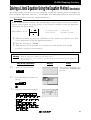
Graphing Calculator
EL-9900
Handbook Vol. 1
Algebra
For Advanced Levels
For Basic Levels
Contents
1. Fractions
1-1
Fractions and Decimals
2. Pie Charts
2-1
Pie Charts and Proportions
3. Linear Equations
3-1
3-2
Slope and Intercept of Linear Equations
Parallel and Perpendicular Lines
4. Quadratic Equations
4-1
Slope and Intercept of Quadratic Equations
5. Literal Equations
5-1
5-2
5-3
Solving a Literal Equation Using the Equation Method (Amortization)
Solving a Literal Equation Using the Graphic Method (Volume of a Cylinder)
Solving a Literal Equation Using Newton’s Method (Area of a Trapezoid)
6. Polynomials
6-1
6-2
Graphing Polynomials and Tracing to Find the Roots
Graphing Polynomials and Jumping to Find the Roots
7. A System of Equations
7-1
Solving a System of Equations by Graphing or Tool Feature
8. Matrix Solutions
8-1
8-2
Entering and Multiplying Matrices
Solving a System of Linear Equations Using Matrices
9. Inequalities
9-1
9-2
9-3
9-4
Solving Inequalities
Solving Double Inequalities
System of Two-Variable Inequalities
Graphing Solution Region of Inequalities
10. Absolute Value Functions, Equations, Inequalities
10-1
10-2
10-3
10-4
Slope and Intercept of Absolute Value Functions
Solving Absolute Value Equations
Solving Absolute Value Inequalities
Evaluating Absolute Value Functions
11. Rational Functions
11-1
11-2
Graphing Rational Functions
Solving Rational Function Inequalities
12. Conic Sections
12-1
12-2
12-3
12-4
Graphing Parabolas
Graphing Circles
Graphing Ellipses
Graphing Hyperbolas
Read this first
1. Always read “Before Starting”
The key operations of the set up conndition are written in “Before Starting” in each section.
It is essential to follow the instructions in order to display the screens as they appear in the
handbook.
2. Set Up Condition
As key operations for this handbook are conducted from the initial condition, reset all memories to the
initial condition beforehand.
2nd F OPTION
E
2
CL
Note: Since all memories will be deleted, it is advised to use the CE-LK2 PC link kit (sold
separately) to back up any programmes not to be erased, or to return the settings to the initial
condition (cf. 3. Initial Settings below) and to erase the data of the function to be used.
• To delete a single data, press 2nd F OPTION C and select data to be deleted from the menu.
• Other keys to delete data:
to erase equations and remove error displays
CL :
to cancel previous function
2nd F QUIT :
3. Initial settings
Initial settings are as follows:
✩ Set up ( 2nd F SET UP ): Advanced keyboard: Rad, FloatPt, 9, Rect, Decimal(Real), Equation, Auto
Basic keyboard: Deg, FloatPt, 9, Rect, Mixed, Equation, Auto
✩ Format ( 2nd F FORMAT ): Advanced keyboard: OFF, OFF, ON, OFF, RectCoord
Basic keyboard: OFF, OFF, ON, OFF
STAT
Stat Plot ( PLOT E ):
2. PlotOFF
Shade ( 2nd F DRAW G ): 2. INITIAL
5. Default
Zoom ( ZOOM A ):
Period ( 2nd F FINANCE C ): 1. PmtEnd (Advanced keyboard only)
Note: ✩ returns to the default setting in the following operation.
( 2nd F OPTION E 1 ENTER )
4. Using the keys
Press 2nd F to use secondary functions (in yellow).
To select “x -1”:
2nd F
x 2 ➔ Displayed as follows:
Press ALPHA to use the alphabet keys (in violet).
To select F:
ALPHA
x 2 ➔ Displayed as follows:
2nd F
x -1
ALPHA
F
5. Notes
• Some features are provided only on the Advanced keyboard and not on the Basic keyboard.
(Solver, Matrix, Tool etc.)
• As this handbook is only an example of how to use the EL-9900, please refer to the manual
for further details.
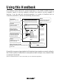
Using this Handbook
This handbook was produced for practical application of the SHARP EL-9900 Graphing
Calculator based on exercise examples received from teachers actively engaged in
teaching. It can be used with minimal preparation in a variety of situations such as
classroom presentations, and also as a self-study reference book.
Introduction
Explanation of the section
Example
Example of a problem to be
solved in the section
Important notes to read
before operating the calculator
Example
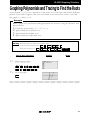
EL-9900 Graphing Calculator
Graph various quadratic equations and check the relation between the graphs and
the values of coefficients of the equations.
1. Graph y = x
2. Graph y = x
3. Graph y = x
4. Graph y = x
Before
Starting
2
and y = (x-2) .
2
and y = x 2+2.
2
and y = 2x 2.
2
and y = -2x 2.
Step & Key Operation
2
Display
Change the equation in Y2 to y = x2+2.
Y=
2nd F
*
2
0
SUB
ENTER
2
GRAPH
1-1
Display
Notes
Enter the equation y = x 2 for Y1.
Y=
X/θ/T/n
3-1
Change the equation in Y2 to y = 2x2.
Y=
Y2 using Sub feature.
Step & Key Operation
ALPHA H
2nd F
(
1-3
0
Notice that the addition of 2 moves
the basic y =x2 graph up two units
and the addition of -2 moves the
basic graph down two units on
the y-axis. This demonstrates the
fact that adding k (>0) within the standard form y = a (x h)2 + k will move the basic graph up k units and placing k
(<0)
k will move the basic graph down k units on the y-axis.
axis.
x2
Enter the equation y = (x-2) 2 for
A
ALPHA
Notes
*Use either pen touch or cursor to operate.
2-1
There may be differences in the results of calculations and graph plotting depending on the setting.
Return all settings to the default value and delete all
-2data.View both graphs.
Step & Key Operation
1-2
A clear step-by-step guide
to solving the problems
Explains the process of each
step in the key operations
A quadratic equation of y in terms of x can be expressed by the standard form y = a (x -h)2+
k, where a is the coefficient of the second degree term ( y = ax 2 + bx + c) and ( h, k) is the
vertex of the parabola formed by the quadratic equation. An equation where the largest
exponent on the independent variable x is 2 is considered a quadratic equation. In graphing
quadratic equations on the calculator, let the x- variable be represented by the horizontal
axis and let y be represented by the vertical axis. The graph can be adjusted by varying the
coefficients a, h, and k.
ENTER
Before Starting
Notes
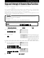
EL-9900 Graphing Calculator
Slope and Intercept of Quadratic Equations
(
X/θ/T/n
x2 +
)
SUB
1
ENTER
)
ALPHA
ENTER
View both graphs.
GRAPH
Display
2
*
0
—
K
3-2
2nd F
SUB
2
ENTER
ENTER
View both graphs.
GRAPH
ENTER
Notice that the addition of -2
within the quadratic operation
moves the basic y =x2 graph
two unitsin(adding
Change right
the equation
Y2 to 2 moves
y = -2x2.it left two units) on the x-axis.
This shows that placing an h (>0) within the standard
2
form y = a (x - h)
+
k
will
move
right
(-) graph
Y=
2nd F the
2
SUB basic
*
h units and placing an h (<0)
will move it left h units
on the x-axis. ENTER
Notice that the multiplication of
2 pinches or closes the basic
y=x2 graph. This demonstrates
the fact that multiplying an a
(> 1) in the standard form y = a
(x - h) 2 + k will pinch or close
the basic graph.
4-1
4-2
View both graphs.
Notice that the multiplication of
-2 pinches or closes the basic
y =x2 graph and flips it (reflects
it) across the x-axis. This demonstrates the fact that multiplying an a (<-1) in the standard form y = a (x - h) 2 + k
will pinch or close the basic graph and flip it (reflect
it) across the x-axis.
4-1
GRAPH
Illustrations of the calculator
screen for each step
The EL-9900 allows various quadratic equations to be graphed easily.
Also the characteristics of quadratic equations can be visually shown through
the relationship between the changes of coefficient values and their graphs,
using the Substitution feature.
Merits of Using the EL-9900
4-1
Highlights the main functions of the calculator relevant
to the section
We would like to express our deepest gratitude to all the teachers whose cooperation we received in editing this
book. We aim to produce a handbook which is more replete and useful to everyone, so any comments or ideas
on exercises will be welcomed.
(Use the attached blank sheet to create and contribute your own mathematical problems.)
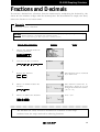
EL-9900 Graphing Calculator
Fractions and Decimals
To convert a decimal into a fraction, form the numerator by multiplying the decimal by 10n,
where n is the number of digits after the decimal point. The denominator is simply 10n. Then,
reduce the fraction to its lowest terms.
Example
Convert 0.75 into a fraction.
Before There may be differences in the results of calculations and graph plotting depending on the setting.
Starting Return all settings to the default value and delete all data.
We recommend using the Basic keyboard to calculate fractions.
Step & Key Operation
1
H
.
7
5
➞b/c
ENTER
ENTER
Enter 3 to further reduce the
fraction.
Simp
5
0
Reduce the fraction.
Simp
4
2
Convert 0.75 into a fraction.
CL
3
Notes
Choose the manual mode for
reducing fractions.
2nd F SET UP
2
Display
3
ENTER
Enter 5 to reduce the fraction.
Simp
5
The fraction can be reduced
by a factor of 5.
The fraction cannot be reduced by a factor of 3, even
though the numerator can be.
(15 = 3 x 5)
0.75 = 3/4
ENTER
○ ○ ○ ○ ○ ○ ○ ○ ○ ○ ○ ○ ○ ○ ○ ○ ○ ○ ○ ○ ○ ○ ○ ○ ○ ○ ○ ○ ○ ○ ○ ○ ○ ○ ○ ○ ○ ○ ○ ○ ○ ○ ○ ○ ○ ○ ○ ○ ○ ○ ○ ○ ○ ○ ○ ○ ○ ○ ○
The EL-9900 can easily convert a decimal into a fraction. It also helps
students learn the steps involved in reducing fractions.
1-1
EL-9900 Graphing Calculator
Pie Charts and Proportions
Pie charts enable a quick and clear overview of how portions of data relate to the whole.
Example
A questionnaire asking students about their favourite colour elicited the following results:
Red:
20 students
Blue: 12 students
Green: 25 students
Pink: 10 students
Yellow: 6 students
1. Make a pie chart based on this data.
2. Find the percentage for each colour.
Before There may be differences in the results of calculations and graph plotting depending on the setting.
Starting Return all settings to the default value and delete all data.
Step & Key Operation
1-1
2
A
ENTER
ENTER
2
6
ENTER
2
5
0
ENTER
ENTER
1
1
0
ENTER
Choose the setting for making a
pie chart.
STAT
PLOT
A
ENTER
STAT
PLOT
1-3
Notes
Enter the data.
STAT
1-2
Display
F
ENTER
1
Make a pie chart.
GRAPH
○ ○ ○ ○ ○ ○ ○ ○ ○ ○ ○ ○ ○ ○ ○ ○ ○ ○ ○ ○ ○ ○ ○ ○ ○ ○ ○ ○ ○ ○ ○ ○ ○ ○ ○ ○ ○ ○ ○ ○ ○ ○ ○ ○ ○ ○ ○ ○ ○ ○ ○ ○ ○ ○ ○ ○ ○ ○ ○
2-1
2-2
Choose the setting for displaying
by percentages.
STAT
PLOT
A
ENTER
STAT
PLOT
F
2
Make another pie chart.
GRAPH
Red:
Blue:
Green:
Pink:
Yellow:
27.39%
16.43%
34.24%
13.69%
8.21%
○ ○ ○ ○ ○ ○ ○ ○ ○ ○ ○ ○ ○ ○ ○ ○ ○ ○ ○ ○ ○ ○ ○ ○ ○ ○ ○ ○ ○ ○ ○ ○ ○ ○ ○ ○ ○ ○ ○ ○ ○ ○ ○ ○ ○ ○ ○ ○ ○ ○ ○ ○ ○ ○ ○ ○ ○ ○ ○
Pie charts can be made easily with the EL-9900.
2-1
EL-9900 Graphing Calculator
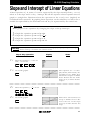
Slope and Intercept of Linear Equations
A linear equation of y in terms of x can be expressed by the slope-intercept form y = mx+b,
where m is the slope and b is the y - intercept. We call this equation a linear equation since its
graph is a straight line. Equations where the exponents on the x and y are 1 (implied) are
considered linear equations. In graphing linear equations on the calculator, we will let the x
variable be represented by the horizontal axis and let y be represented by the vertical axis.
Example
Draw graphs of two equations by changing the slope or the y- intercept.
1. Graph the equations y = x and y = 2x.
2. Graph the equations y = x and y = 12 x.
3. Graph the equations y = x and y = - x.
4. Graph the equations y = x and y = x + 2.
Before There may be differences in the results of calculations and graph plotting depending on the setting.
Starting Return all settings to the default value and delete all data.
Step & Key Operation
1-1
Notes
Enter the equation y = x for Y1
and y = 2x for Y2.
Y=
1-2
Display
X/ /T/n
ENTER
2
X/ /T/n
View both graphs.
The equation Y1 = x is displayed first, followed by the
equation Y2 = 2x. Notice how
Y2 becomes steeper or climbs
faster. Increase the size of the
slope (m>1) to make the line
steeper.
GRAPH
○ ○ ○ ○ ○ ○ ○ ○ ○ ○ ○ ○ ○ ○ ○ ○ ○ ○ ○ ○ ○ ○ ○ ○ ○ ○ ○ ○ ○ ○ ○ ○ ○ ○ ○ ○ ○ ○ ○ ○ ○ ○ ○ ○ ○ ○ ○ ○ ○ ○ ○ ○ ○ ○ ○ ○ ○ ○ ○
2-1
Enter the equation y = 12 x for Y2.
Y=
1
2-2
CL
a/b
2
View both graphs.
GRAPH
X/ /T/n
Notice how Y2 becomes less
steep or climbs slower. Decrease the size of the slope
(0<m<1) to make the line less
steep.
○ ○ ○ ○ ○ ○ ○ ○ ○ ○ ○ ○ ○ ○ ○ ○ ○ ○ ○ ○ ○ ○ ○ ○ ○ ○ ○ ○ ○ ○ ○ ○ ○ ○ ○ ○ ○ ○ ○ ○ ○ ○ ○ ○ ○ ○ ○ ○ ○ ○ ○ ○ ○ ○ ○ ○ ○ ○ ○
3-1
EL-9900 Graphing Calculator
Step & Key Operation
3-1
Notes
Enter the equation y = - x for Y2.
Y=
3-2
Display
CL
(-)
X/ /T/n
View both graphs.
Notice how Y2 decreases
(going down from left to
right) instead of increasing
(going up from left to right).
Negative slopes (m<0) make
the line decrease or go
down from left to right.
GRAPH
○ ○ ○ ○ ○ ○ ○ ○ ○ ○ ○ ○ ○ ○ ○ ○ ○ ○ ○ ○ ○ ○ ○ ○ ○ ○ ○ ○ ○ ○ ○ ○ ○ ○ ○ ○ ○ ○ ○ ○ ○ ○ ○ ○ ○ ○ ○ ○ ○ ○ ○ ○ ○ ○ ○ ○ ○ ○ ○
4-1
Enter the equation y = x + 2 for
Y2.
Y=
4-2
CL
X/ /T/n
View both graphs.
GRAPH
+
2
Adding 2 will shift the y = x
graph upwards.
○ ○ ○ ○ ○ ○ ○ ○ ○ ○ ○ ○ ○ ○ ○ ○ ○ ○ ○ ○ ○ ○ ○ ○ ○ ○ ○ ○ ○ ○ ○ ○ ○ ○ ○ ○ ○ ○ ○ ○ ○ ○ ○ ○ ○ ○ ○ ○ ○ ○ ○ ○ ○ ○ ○ ○ ○ ○ ○
Making a graph is easy, and quick comparison of several graphs will help
students understand the characteristics of linear equations.
3-1
EL-9900 Graphing Calculator
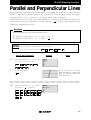
Parallel and Perpendicular Lines
Parallel and perpendicular lines can be drawn by changing the slope of the linear equation
and the y intercept. A linear equation of y in terms of x can be expressed by the slopeintercept form y = mx + b, where m is the slope and b is the y-intercept.
Parallel lines have an equal slope with different y-intercepts. Perpendicular lines have
1 ). These characteristics can be
slopes that are negative reciprocals of each other (m = - m
verified by graphing these lines.
Example
Graph parallel lines and perpendicular lines.
1. Graph the equations y = 3x + 1 and y = 3x + 2.
2. Graph the equations y = 3x - 1 and y = - 31 x + 1.
Before There may be differences in the results of calculations and graph plotting depending on the setting.
Starting Return all settings to the default value and delete all data.
Set the zoom to the decimal window: ZOOM
Step & Key Operation
1-1
Display
) 7
Notes
Enter the equations y = 3x + 1 for
Y1 and y = 3x + 2 for Y2.
Y=
3
1-2
C ( ENTER ALPHA
3
X/ /T/n
X/ /T/n
+
+
1
ENTER
2
View the graphs.
These lines have an equal
slope but different y-intercepts.
They are called parallel, and
will not intersect.
GRAPH
○ ○ ○ ○ ○ ○ ○ ○ ○ ○ ○ ○ ○ ○ ○ ○ ○ ○ ○ ○ ○ ○ ○ ○ ○ ○ ○ ○ ○ ○ ○ ○ ○ ○ ○ ○ ○ ○ ○ ○ ○ ○ ○ ○ ○ ○ ○ ○ ○ ○ ○ ○ ○ ○ ○ ○ ○ ○ ○
2-1
Enter the equations y = 3x - 1 for
Y1 and y = - 1 x + 1 for Y2.
3
Y=
CL
3
X/ /T/n
—
CL
(-)
1
a/b
3
+
1
1
ENTER
X/ /T/n
3-2
EL-9900 Graphing Calculator
Step & Key Operation
2-2
View the graphs.
GRAPH
Display
Notes
These lines have slopes that
are negative reciprocals of
each other (m = - 1 ). They are
m
called perpendicular. Note that
these intersecting lines form
four equal angles.
○ ○ ○ ○ ○ ○ ○ ○ ○ ○ ○ ○ ○ ○ ○ ○ ○ ○ ○ ○ ○ ○ ○ ○ ○ ○ ○ ○ ○ ○ ○ ○ ○ ○ ○ ○ ○ ○ ○ ○ ○ ○ ○ ○ ○ ○ ○ ○ ○ ○ ○ ○ ○ ○ ○ ○ ○ ○ ○
The Graphing Calculator can be used to draw parallel or perpendicular
lines while learning the slope or y-intercept of linear equations.
3-2
EL-9900 Graphing Calculator
Slope and Intercept of Quadratic Equations
A quadratic equation of y in terms of x can be expressed by the standard form y = a (x - h) 2+ k,
where a is the coefficient of the second degree term (y = ax 2 + bx + c) and (h, k) is the
vertex of the parabola formed by the quadratic equation. An equation where the largest
exponent on the independent variable x is 2 is considered a quadratic equation. In graphing
quadratic equations on the calculator, let the x-variable be represented by the horizontal
axis and let y be represented by the vertical axis. The graph can be adjusted by varying the
coefficients a, h, and k.
Example
Graph various quadratic equations and check the relation between the graphs and
the values of coefficients of the equations.
1. Graph y = x
2. Graph y = x
3. Graph y = x
4. Graph y = x
2
2
2
2
and y = (x - 2) 2.
and y = x 2 + 2.
and y = 2x 2.
and y = - 2x 2.
Before There may be differences in the results of calculations and graph plotting depending on the setting.
Starting Return all settings to the default value and delete all data.
Step & Key Operation
1-1
x2
X/ /T/n
Enter the equation y = (x - 2) 2 for
Y2 using Sub feature.
A
ALPHA
1-3
Notes
Enter the equation y = x 2 for Y1.
Y=
1-2
Display
H
2nd F
SUB
(
ENTER
0
1
ENTER
ALPHA
2
—
K
ENTER
)
View both graphs.
GRAPH
X/ /T/n
x2 +
)
ALPHA
(
Notice that the addition of -2
within the quadratic operation
moves the basic y = x 2 graph
right two units (adding 2 moves
it left two units) on the x-axis.
This shows that placing an h (>0) within the standard
form y = a (x - h) 2 + k will move the basic graph right
h units and placing an h (<0) will move it left h units
on the x-axis.
○ ○ ○ ○ ○ ○ ○ ○ ○ ○ ○ ○ ○ ○ ○ ○ ○ ○ ○ ○ ○ ○ ○ ○ ○ ○ ○ ○ ○ ○ ○ ○ ○ ○ ○ ○ ○ ○ ○ ○ ○ ○ ○ ○ ○ ○ ○ ○ ○ ○ ○ ○ ○ ○ ○ ○ ○ ○
4-1
EL-9900 Graphing Calculator
Step & Key Operation
2-1
Notes
Change the equation in Y2 to y = x 2+2.
Y=
2nd F
2
ENTER
2-2
Display
0
SUB
ENTER
View both graphs.
Notice that the addition of 2 moves
the basic y = x 2 graph up two units
and the addition of - 2 moves the
basic graph down two units on
the y-axis. This demonstrates the
fact that adding k (>0) within the standard form y = a (x h) 2 + k will move the basic graph up k units and placing k
(<0) will move the basic graph down k units on the y-axis.
GRAPH
○ ○ ○ ○ ○ ○ ○ ○ ○ ○ ○ ○ ○ ○ ○ ○ ○ ○ ○ ○ ○ ○ ○ ○ ○ ○ ○ ○ ○ ○ ○ ○ ○ ○ ○ ○ ○ ○ ○ ○ ○ ○ ○ ○ ○ ○ ○ ○ ○ ○ ○ ○ ○ ○ ○ ○ ○ ○
3-1
Change the equation in Y2 to y = 2x 2.
Y=
2nd F
0
3-2
SUB
2
ENTER
ENTER
Notice that the multiplication of
2 pinches or closes the basic
y = x 2 graph. This demonstrates
the fact that multiplying an a
(> 1) in the standard form y = a
(x - h) 2 + k will pinch or close
the basic graph.
View both graphs.
GRAPH
○ ○ ○ ○ ○ ○ ○ ○ ○ ○ ○ ○ ○ ○ ○ ○ ○ ○ ○ ○ ○ ○ ○ ○ ○ ○ ○ ○ ○ ○ ○ ○ ○ ○ ○ ○ ○ ○ ○ ○ ○ ○ ○ ○ ○ ○ ○ ○ ○ ○ ○ ○ ○ ○ ○ ○ ○ ○
4-1
Change the equation in Y2 to
y = - 2x 2.
Y=
2nd F
SUB
(-)
2
ENTER
4-2
View both graphs.
GRAPH
Notice that the multiplication of
-2 pinches or closes the basic
y =x 2 graph and flips it (reflects
it) across the x-axis. This demonstrates the fact that multiplying an a (<-1) in the standard form y = a (x - h) 2 + k
will pinch or close the basic graph and flip it (reflect
it) across the x-axis.
○ ○ ○ ○ ○ ○ ○ ○ ○ ○ ○ ○ ○ ○ ○ ○ ○ ○ ○ ○ ○ ○ ○ ○ ○ ○ ○ ○ ○ ○ ○ ○ ○ ○ ○ ○ ○ ○ ○ ○ ○ ○ ○ ○ ○ ○ ○ ○ ○ ○ ○ ○ ○ ○ ○ ○ ○ ○
The EL-9900 allows various quadratic equations to be graphed easily. Also the
characteristics of quadratic equations can be visually shown through the
relationship between the changes of coefficient values and their graphs, using
the Substitution feature.
4-1
EL-9900 Graphing Calculator
Solving a Literal Equation Using the Equation Method (Amortization)
The Solver mode is used to solve one unknown variable by inputting known variables, by
three methods: Equation, Newton’s, and Graphic. The Equation method is used when an
exact solution can be found by simple substitution.
Example
Solve an amortization formula. The solution from various values for known variables
can be easily found by giving values to the known variables using the Equation
method in the Solver mode.
The formula : P = L
I -N
1-(1+ 12 )
I
12
-1
P= monthly payment
L= loan amount
I= interest rate
N=number of months
1. Find the monthly payment on a $15,000 car loan, made at 9% interest over four
2.
3.
years (48 months) using the Equation method.
Save the formula as “AMORT”.
Find amount of loan possible at 7% interest over 60 months with a $300
payment, using the saved formula.
Before
Starting
There may be differences in the results of calculations and graph plotting depending on the setting.
Return all settings to the default value and delete all data.
As the Solver feature is only available on the Advanced keyboard, this section does not apply to the
Basic keyboard.
Step & Key Operation
1-1
Display
Access the Solver feature.
This screen will appear a few
seconds after “SOLVER” is displayed.
2nd F SOLVER
1-2
Notes
Select the Equation method for
solving.
2nd F SOLVER
A
1
1-3
Enter the amortization formula.
2nd F ALPHA
P
=
a/b
1
—
(
ALPHA
ab
I
(-)
a/b
1
ALPHA
N
ALPHA
I
a/b
1
)
ab
(-)
1
L ALPHA
(
2
+
1
)
2
5-1
EL-9900 Graphing Calculator
Step & Key Operation
1-4
Notes
Enter the values L=15,000,
I=0.09, N=48.
1
ENTER
ENTER
8
1-5
Display
•
0
5
9
0
0
ENTER
0
4
ENTER
The monthly payment (P) is
$373.28.
Solve for the payment(P).
2nd F
(
CL
EXE
)
○ ○ ○ ○ ○ ○ ○ ○ ○ ○ ○ ○ ○ ○ ○ ○ ○ ○ ○ ○ ○ ○ ○ ○ ○ ○ ○ ○ ○ ○ ○ ○ ○ ○ ○ ○ ○ ○ ○ ○ ○ ○ ○ ○ ○ ○ ○ ○ ○ ○ ○ ○ ○ ○ ○ ○ ○ ○
2-1
Save this formula.
2nd F SOLVER
2-2
C
ENTER
Give the formula the name AMORT.
A
M
O
R
T
ENTER
○ ○ ○ ○ ○ ○ ○ ○ ○ ○ ○ ○ ○ ○ ○ ○ ○ ○ ○ ○ ○ ○ ○ ○ ○ ○ ○ ○ ○ ○ ○ ○ ○ ○ ○ ○ ○ ○ ○ ○ ○ ○ ○ ○ ○ ○ ○ ○ ○ ○ ○ ○ ○ ○ ○ ○ ○ ○
3-1
Recall the amortization formula.
2nd F SOLVER
0
3-2
3-3
B
1
Enter the values: P = 300,
I = 0.01, N = 60
ENTER
3
0
•
1
ENTER
0
0
ENTER
0
6
ENTER
Solve for the loan (L).
2nd F
0
ENTER
The amount of loan (L) is
$17550.28.
EXE
○ ○ ○ ○ ○ ○ ○ ○ ○ ○ ○ ○ ○ ○ ○ ○ ○ ○ ○ ○ ○ ○ ○ ○ ○ ○ ○ ○ ○ ○ ○ ○ ○ ○ ○ ○ ○ ○ ○ ○ ○ ○ ○ ○ ○ ○ ○ ○ ○ ○ ○ ○ ○ ○ ○ ○ ○ ○
With the Equation Editor, the EL-9900 displays equations, even complicated
ones, as they appear in the textbook in easy to understand format. Also it is
easy to find the solution for unknown variables by recalling a stored equation
and giving values to the known variables in the Solver mode when using the
Advanced keyboard.
5-1
EL-9900 Graphing Calculator
Solving a Literal Equation Using the Graphic Method (Volume of a Cylinder)
The Solver mode is used to solve one unknown variable by inputting known variables.
There are three methods: Equation, Newton’s, and Graphic. The Equation method is used
when an exact solution can be found by simple substitution. Newton’s method implements
an iterative approach to find the solution once a starting point is given. When a starting
point is unavailable or multiple solutions are expected, use the Graphic method. This
method plots the left and right sides of the equation and then locates the intersection(s).
Example
Use the Graphic method to find the radius of a cylinder giving the range of the unknown
variable.
The formula : V = πr 2h
( V = volume
r = radius
h = height)
1. Find the radius of a cylinder with a volume of 30in
3
2.
3.
and a height of 10in, using
the Graphic method.
Save the formula as “V CYL”.
Find the radius of a cylinder with a volume of 200in 3 and a height of 15in,
using the saved formula.
Before There may be differences in the results of calculations and graph plotting depending on the setting.
Starting Return all settings to the default value and delete all data.
As the Solver feature is only available on the Advanced keyboard, this section does not apply to the
Basic keyboard.
Step & Key Operation
1-1
Display
Access the Solver feature.
This screen will appear a few
seconds after “SOLVER” is displayed.
2nd F SOLVER
1-2
Notes
Select the Graphic method for
solving.
2nd F SOLVER
A
3
1-3
Enter the formula V = πr 2h.
V
ALPHA
R
1-4
x2
=
ALPHA
ALPHA
2nd F
π
ALPHA
H
Enter the values: V = 30, H = 10.
Solve for the radius (R).
ENTER
0
3
ENTER
0
1
ENTER
2nd F
EXE
5-2
EL-9900 Graphing Calculator
Step & Key Operation
1-5
Set the variable range from 0 to 2.
0
2
ENTER
Notes
Display
ENTER
The graphic solver will prompt
with a variable range for solving.
30
3
=
<3
π
10π
r =1 ➞ r 2 = 12 = 1 <3
r =2 ➞ r 2 = 22 = 4 >3
r2=
Use the larger of the values to
be safe.
1-6
The solver feature will graph
the left side of the equation
(volume, y = 30), then the right
side of the equation (y = 10r 2),
and finally will calculate the
intersection of the two graphs
to find the solution.
The radius is 0.98 in.
Solve.
2nd F
EXE
(
CL
)
○ ○ ○ ○ ○ ○ ○ ○ ○ ○ ○ ○ ○ ○ ○ ○ ○ ○ ○ ○ ○ ○ ○ ○ ○ ○ ○ ○ ○ ○ ○ ○ ○ ○ ○ ○ ○ ○ ○ ○ ○ ○ ○ ○ ○ ○ ○ ○ ○ ○ ○ ○ ○ ○ ○ ○ ○ ○ ○
2
Save this formula.
Give the formula the name “V CYL”.
C
2nd F SOLVER
V
SPACE
C
ENTER
Y
L
ENTER
○ ○ ○ ○ ○ ○ ○ ○ ○ ○ ○ ○ ○ ○ ○ ○ ○ ○ ○ ○ ○ ○ ○ ○ ○ ○ ○ ○ ○ ○ ○ ○ ○ ○ ○ ○ ○ ○ ○ ○ ○ ○ ○ ○ ○ ○ ○ ○ ○ ○ ○ ○ ○ ○ ○ ○ ○ ○ ○
3-1
Recall the formula.
Enter the values: V = 200, H = 15.
2nd F SOLVER
3-2
B
0
1
0
0
ENTER
ENTER
2
1
ENTER
5
0
ENTER
Solve the radius setting the variable
range from 0 to 4.
2nd F
ENTER
2nd F
EXE
EXE
0
ENTER
4
200
14
= < 14
π
15π
2
r = 3 ➞ r = 32 = 9 < 14
r = 4 ➞ r 2 = 42 = 16 > 14
r2=
Use 4, the larger of the values,
to be safe.
The answer is : r = 2.06
○ ○ ○ ○ ○ ○ ○ ○ ○ ○ ○ ○ ○ ○ ○ ○ ○ ○ ○ ○ ○ ○ ○ ○ ○ ○ ○ ○ ○ ○ ○ ○ ○ ○ ○ ○ ○ ○ ○ ○ ○ ○ ○ ○ ○ ○ ○ ○ ○ ○ ○ ○ ○ ○ ○ ○ ○ ○ ○
One very useful feature of the calculator is its ability to store and recall equations.
The solution from various values for known variables can be easily obtained by
recalling an equation which has been stored and giving values to the known
variables. The Graphic method gives a visual solution by drawing a graph.
5-2
EL-9900 Graphing Calculator
Solving a Literal Equation Using Newton's Method (Area of a Trapezoid)
The Solver mode is used to solve one unknown variable by inputting known variables.
There are three methods: Equation, Newton’s, and Graphic. The Newton’s method can
be used for more complicated equations. This method implements an iterative approach
to find the solution once a starting point is given.
Example
Find the height of a trapezoid from the formula for calculating the area of a trapezoid
using Newton’s method.
1
The formula : A= h(b+c) (A = area h = height b = top face c = bottom face)
2
1. Find the height of a trapezoid with an area of 25in
2
2.
3.
and bases of length 5in
and 7in using Newton's method. (Set the starting point to 1.)
Save the formula as “A TRAP”.
Find the height of a trapezoid with an area of 50in2 with bases of 8in and 10in
using the saved formula. (Set the starting point to 1.)
Before There may be differences in the results of calculations and graph plotting depending on the setting.
Starting Return all settings to the default value and delete all data.
As the Solver feature is only available on the Advanced keyboard, this section does not apply to the
Basic keyboard.
Step & Key Operation
1-1
Display
Access the Solver feature.
This screen will appear a few
seconds after “SOLVER” is displayed.
2nd F SOLVER
1-2
Notes
Select Newton's method
for solving.
2nd F SOLVER
A
2
1-3
1-4
Enter the formula A = 21 h(b+c).
ALPHA
A ALPHA
ALPHA
H
C
)
(
=
1
ALPHA
B
a/b
+
2
ALPHA
Enter the values: A = 25, B = 5, C = 7
2
ENTER
5
5
ENTER
ENTER
7
ENTER
5-3
EL-9900 Graphing Calculator
Step & Key Operation
1-5
Solve for the height and enter a
starting point of 1.
2nd F
1-6
Display
1
EXE
Newton's method will
prompt with a guess or a
starting point.
ENTER
The answer is : h = 4.17
Solve.
2nd F
Notes
EXE
(
CL
)
○ ○ ○ ○ ○ ○ ○ ○ ○ ○ ○ ○ ○ ○ ○ ○ ○ ○ ○ ○ ○ ○ ○ ○ ○ ○ ○ ○ ○ ○ ○ ○ ○ ○ ○ ○ ○ ○ ○ ○ ○ ○ ○ ○ ○ ○ ○ ○ ○ ○ ○ ○ ○ ○ ○ ○ ○ ○ ○
2
Save this formula. Give the formula
the name “A TRAP”.
C
2nd F SOLVER
A
SPACE
ENTER
A
R
T
P
ENTER
○ ○ ○ ○ ○ ○ ○ ○ ○ ○ ○ ○ ○ ○ ○ ○ ○ ○ ○ ○ ○ ○ ○ ○ ○ ○ ○ ○ ○ ○ ○ ○ ○ ○ ○ ○ ○ ○ ○ ○ ○ ○ ○ ○ ○ ○ ○ ○ ○ ○ ○ ○ ○ ○ ○ ○ ○ ○ ○
3-1
Recall the formula for calculating
the area of a trapezoid.
2nd F SOLVER
0
3-2
3-3
B
1
Enter the values:
A = 50, B = 8, C = 10.
ENTER
5
0
ENTER
ENTER
1
0
ENTER
8
Solve.
The answer is : h = 5.56
2nd F
ENTER
2nd F
EXE
1
EXE
○ ○ ○ ○ ○ ○ ○ ○ ○ ○ ○ ○ ○ ○ ○ ○ ○ ○ ○ ○ ○ ○ ○ ○ ○ ○ ○ ○ ○ ○ ○ ○ ○ ○ ○ ○ ○ ○ ○ ○ ○ ○ ○ ○ ○ ○ ○ ○ ○ ○ ○ ○ ○ ○ ○ ○ ○ ○ ○
One very useful feature of the calculator is its ability to store and recall equations.
The solution from various values for known variables can be easily obtained by
recalling an equation which has been stored and giving values to the known
variables in the Solver mode. If a starting point is known, Newton's method is
useful for quick solution of a complicated equation.
5-3
EL-9900 Graphing Calculator
Graphing Polynomials and Tracing to Find the Roots
A polynomial y = f (x) is an expression of the sums of several terms that contain different
powers of the same originals. The roots are found at the intersection of the x-axis and
the graph, i. e. when y = 0.
Example
Draw a graph of a polynomial and approximate the roots by using the Zoom-in and
Trace features.
1. Graph the polynomial y = x - 3x
2. Approximate the left-hand root.
3. Approximate the middle root.
4. Approximate the right-hand root.
3
2
+ x + 1.
Before There may be differences in the results of calculations and graph plotting depending on the setting.
Starting Return all settings to the default value and delete all data.
) 7
Set the zoom to the decimal window: ZOOM A ( ENTER ALPHA
Setting the zoom factors to 5 : ZOOM B
Step & Key Operation
1-1
5
ENTER
Display
5
ENTER 2nd F QUIT
Notes
Enter the polynomial
y = x 3 - 3x 2 + x + 1.
Y=
X/ /T/n
1-2
ENTER
X/ /T/n
ab
3
x2
+
X/ /T/n
—
+
3
1
View the graph.
GRAPH
○ ○ ○ ○ ○ ○ ○ ○ ○ ○ ○ ○ ○ ○ ○ ○ ○ ○ ○ ○ ○ ○ ○ ○ ○ ○ ○ ○ ○ ○ ○ ○ ○ ○ ○ ○ ○ ○ ○ ○ ○ ○ ○ ○ ○ ○ ○ ○ ○ ○ ○ ○ ○ ○ ○ ○ ○ ○ ○
6-1
EL-9900 Graphing Calculator
Step & Key Operation
2-1
Tracer
(repeatedly)
Zoom in on the left-hand root.
ZOOM
2-3
Note that the tracer is flashing
on the curve and the x and y
coordinates are shown at the
bottom of the screen.
Move the tracer near the left-hand
root.
TRACE
2-2
Notes
Display
A
3
Tracer
Move the tracer to approximate the
root.
or
TRACE
The root is : x
-0.42
(repeatedly)
○ ○ ○ ○ ○ ○ ○ ○ ○ ○ ○ ○ ○ ○ ○ ○ ○ ○ ○ ○ ○ ○ ○ ○ ○ ○ ○ ○ ○ ○ ○ ○ ○ ○ ○ ○ ○ ○ ○ ○ ○ ○ ○ ○ ○ ○ ○ ○ ○ ○ ○ ○ ○ ○ ○ ○ ○ ○ ○
3-1
Return to the previous decimal
viewing window.
ZOOM
H
2
3-2
Tracer
Move the tracer to approximate
the middle root.
TRACE
The root is exactly x = 1.
(Zooming is not needed to
find a better approximate.)
(repeatedly)
○ ○ ○ ○ ○ ○ ○ ○ ○ ○ ○ ○ ○ ○ ○ ○ ○ ○ ○ ○ ○ ○ ○ ○ ○ ○ ○ ○ ○ ○ ○ ○ ○ ○ ○ ○ ○ ○ ○ ○ ○ ○ ○ ○ ○ ○ ○ ○ ○ ○ ○ ○ ○ ○ ○ ○ ○ ○
4
Tracer
Move the tracer near the righthand root.
Zoom in and move the tracer to
find a better approximate.
The root is : x
2.42
(repeatedly)
ZOOM
TRACE
A
3
or
(repeatedly)
○ ○ ○ ○ ○ ○ ○ ○ ○ ○ ○ ○ ○ ○ ○ ○ ○ ○ ○ ○ ○ ○ ○ ○ ○ ○ ○ ○ ○ ○ ○ ○ ○ ○ ○ ○ ○ ○ ○ ○ ○ ○ ○ ○ ○ ○ ○ ○ ○ ○ ○ ○ ○ ○ ○ ○ ○ ○ ○
The calculator allows the roots to be found (or approximated) visually by
graphing a polynomial and using the Zoom-in and Trace features.
6-1
EL-9900 Graphing Calculator
Graphing Polynomials and Jumping to Find the Roots
A polynomial y = f (x) is an expression of the sums of several terms that contain different
powers of the same originals. The roots are found at the intersection of the x- axis and the
graph, i. e. when y = 0.
Example
Draw a graph of a polynomial and find the roots by using the Calculate feature.
1. Graph the polynomial y = x + x
2. Find the four roots one by one.
4
3
- 5x 2 - 3x + 1.
Before There may be differences in the results of calculations and graph plotting depending on the setting.
Starting Return all settings to the default value and delete all data.
Setting the zoom factors to 5 : ZOOM
Step & Key Operation
1-1
ENTER
A
ENTER
A
ENTER
Display
2nd F QUIT
Notes
Enter the polynomial
y = x 4 + x 3 - 5x 2 - 3x + 1
X/ /T/n
Y=
ab
—
1-2
A
5 X/ /T/n
—
3
3
+
ab 4
X/ /T/n
+
X/ /T/n
x2
1
View the graph.
GRAPH
○ ○ ○ ○ ○ ○ ○ ○ ○ ○ ○ ○ ○ ○ ○ ○ ○ ○ ○ ○ ○ ○ ○ ○ ○ ○ ○ ○ ○ ○ ○ ○ ○ ○ ○ ○ ○ ○ ○ ○ ○ ○ ○ ○ ○ ○ ○ ○ ○ ○ ○ ○ ○ ○ ○ ○ ○ ○
2-1
Find the first root.
2nd F CALC
5
x -2.47
Y is almost but not exactly zero.
Notice that the root found here
is an approximate value.
2-2
Find the next root.
2nd F CALC
x
-0.82
5
6-2
EL-9900 Graphing Calculator
Step & Key Operation
2-3
Find the next root.
2nd F
2-4
CALC
CALC
x
0.24
x
2.05
5
Find the next root.
2nd F
Notes
Display
5
○ ○ ○ ○ ○ ○ ○ ○ ○ ○ ○ ○ ○ ○ ○ ○ ○ ○ ○ ○ ○ ○ ○ ○ ○ ○ ○ ○ ○ ○ ○ ○ ○ ○ ○ ○ ○ ○ ○ ○ ○ ○ ○ ○ ○ ○ ○ ○ ○ ○ ○ ○ ○ ○ ○ ○ ○ ○ ○
The calculator allows jumping to find the roots by graphing a polynomial
and using the Calculate feature, without tracing the graph.
6-2
EL-9900 Graphing Calculator
Solving a System of Equations by Graphing or Tool Feature
A system of equations is made up of two or more equations. The calculator provides the
Calculate feature and Tool feature to solve a system of equations. The Calculate feature
finds the solution by calculating the intersections of the graphs of equations and is useful
for solving a system when there are two variables, while the Tool feature can solve a linear
system with up to six variables and six equations.
Example
Solve a system of equations using the Calculate or Tool feature. First, use the Calculate feature. Enter the equations, draw the graph, and find the intersections. Then,
use the Tool feature to solve a system of equations.
1. Solve the system using the Calculate feature.
{
y = x2- 1
y = 2x
2. Solve the system using the Tool feature.
{
5x + y = 1
-3x + y = -5
Before There may be differences in the results of calculations and graph plotting depending on the setting.
Starting Return all settings to the default value and delete all data.
Set viewing window to “-5 < X < 5”, “-10 < Y < 10”.
(-)
WINDOW
5 ENTER 5 ENTER
As the Tool feature is only available on the Advanced keyboard, example 2 does not apply to the
Basic keyboard.
Step & Key Operation
1-1
Display
Notes
Enter the system of equations
y = x 2 - 1 for Y1 and y = 2x for Y2.
Y=
X/ /T/n
x2
—
1
ENTER
2 X/ /T/n
1-2
View the graphs.
GRAPH
1-3
Find the left-hand intersection using
the Calculate feature.
2nd F CALC
1-4
2
Find the right-hand intersection by
accessing the Calculate feature again.
2nd F CALC
Note that the x and y coordinates are shown at the bottom of the screen. The answer
is : x = - 0.41 y = - 0.83
The answer is : x = 2.41
y = 4.83
2
○ ○ ○ ○ ○ ○ ○ ○ ○ ○ ○ ○ ○ ○ ○ ○ ○ ○ ○ ○ ○ ○ ○ ○ ○ ○ ○ ○ ○ ○ ○ ○ ○ ○ ○ ○ ○ ○ ○ ○ ○ ○ ○ ○ ○ ○ ○ ○ ○ ○ ○ ○ ○ ○ ○ ○ ○ ○ ○
7-1
EL-9900 Graphing Calculator
Step & Key Operation
2-1
Access the Tool menu. Select the
number of variables.
2nd F
2-2
TOOL
B
Notes
Display
Using the system function, it
is possible to solve simultaneous linear equations. Systems up to six variables and
six equations can be solved.
2
Enter the system of equations.
5
ENTER
1
ENTER
1
3
ENTER
1
ENTER
(-)
ENTER
(-)
5
ENTER
2-3
Solve the system.
2nd F
x = 0.75
y = - 2.75
EXE
○ ○ ○ ○ ○ ○ ○ ○ ○ ○ ○ ○ ○ ○ ○ ○ ○ ○ ○ ○ ○ ○ ○ ○ ○ ○ ○ ○ ○ ○ ○ ○ ○ ○ ○ ○ ○ ○ ○ ○ ○ ○ ○ ○ ○ ○ ○ ○ ○ ○ ○ ○ ○ ○ ○ ○ ○ ○ ○
A system of equations can be solved easily by using the Calculate feature
or Tool feature.
7-1
EL-9900 Graphing Calculator
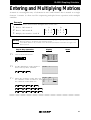
Entering and Multiplying Matrices
A matrix is a rectangular array of elements in rows and columns that is treated as a single
element. A matrix is often used for expressing multiple linear equations with multiple
variables.
Example
Enter two matrices and execute multiplication of the two.
A
Enter a 3 x 3 matrix A
1 2 1
1
Enter a 3 x 3 matrix B
2 1 -1
4
1 1 -2
7
Multiply the matrices A and B
1.
2.
3.
B
2 3
5 6
8 9
Before There may be differences in the results of calculations and graph plotting depending on the setting.
Starting Return all settings to the default value and delete all data.
As the Matrix feature is only available on the Advanced keyboard, this section does not apply to the
Basic keyboard.
Step & Key Operation
1-1
Display
Notes
Access the matrix menu.
2nd F
MATRIX
B
1
1-2
Set the dimension of the matrix at
three rows by three columns.
3
1-3
ENTER
3
ENTER
Enter the elements of the first row,
the elements of the second row, and
the elements of the third row.
1
ENTER
2
ENTER
1
2
ENTER
1
ENTER
(-)
1
ENTER
1
ENTER
1
ENTER
(-)
2
ENTER
ENTER
○ ○ ○ ○ ○ ○ ○ ○ ○ ○ ○ ○ ○ ○ ○ ○ ○ ○ ○ ○ ○ ○ ○ ○ ○ ○ ○ ○ ○ ○ ○ ○ ○ ○ ○ ○ ○ ○ ○ ○ ○ ○ ○ ○ ○ ○ ○ ○ ○ ○ ○ ○ ○ ○ ○ ○ ○ ○ ○
8-1
EL-9900 Graphing Calculator
Step & Key Operation
2
Notes
Display
Enter a 3 x 3 matrix B.
3
3
MATRIX
B
2
1
ENTER
2
ENTER
3
ENTER
4
ENTER
5
ENTER
6
ENTER
7
ENTER
8
ENTER
9
ENTER
2nd F
ENTER
ENTER
○ ○ ○ ○ ○ ○ ○ ○ ○ ○ ○ ○ ○ ○ ○ ○ ○ ○ ○ ○ ○ ○ ○ ○ ○ ○ ○ ○ ○ ○ ○ ○ ○ ○ ○ ○ ○ ○ ○ ○ ○ ○ ○ ○ ○ ○ ○ ○ ○ ○ ○ ○ ○ ○ ○ ○ ○ ○ ○
3-1
Multiply the matrices A and B
together at the home screen.
2nd F
A
2
MATRIX
A
1
X
ENTER
2nd F
MATRIX
Matrix multiplication can
be performed if the number of columns of the first
matrix is equal to the number of rows of the second
matrix. The sum of these
multiplications (1 1 + 2 4
+ 1 7) is placed in the 1,1
(first row, first column) position of the resulting matrix. This process is repeated until each row of A
has been multiplied by
each column of B.
.
3-2
.
.
Delete the input matrices for
future use.
2nd F OPTION
C
2
ENTER
2nd F
ENTER
QUIT
○ ○ ○ ○ ○ ○ ○ ○ ○ ○ ○ ○ ○ ○ ○ ○ ○ ○ ○ ○ ○ ○ ○ ○ ○ ○ ○ ○ ○ ○ ○ ○ ○ ○ ○ ○ ○ ○ ○ ○ ○ ○ ○ ○ ○ ○ ○ ○ ○ ○ ○ ○ ○ ○ ○ ○ ○ ○ ○
Matrix multiplication can be performed easily by the calculator.
8-1
EL-9900 Graphing Calculator
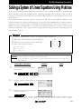
Solving a System of Linear Equations Using Matrices
Each system of three linear equations consists of three variables. Equations in more than
three variables cannot be graphed on the graphing calculator. The solution of the system of
equations can be found numerically using the Matrix feature or the System solver in the
Tool feature.
A system of linear equations can be expressed as AX = B (A, X and B are matrices). The
solution matrix X is found by multiplying A-1 B. Note that the multiplication is “order sensitive”
and the correct answer will be obtained by multiplying BA-1. An inverse matrix A-1 is a
matrix that when multiplied by A results in the identity matrix I (A-1 x A=I). The identity
matrix I is defined to be a square matrix (n x n) where each position on the diagonal is 1
and all others are 0.
Example
Use matrix multiplication to solve a system of linear equations.
B
Enter the 3 x 3 identity matrix in matrix A.
1 2 1
Find the inverse matrix of the matrix B.
2 1 -1
Solve the equation system.
1 1 -2
x + 2y + z = 8
2x + y - z = 1
x + y - 2z = -3
1.
2.
3.
{
Before There may be differences in the results of calculations and graph plotting depending on the setting.
Starting Return all settings to the default value and delete all data.
As the Matrix feature is only available on the Advanced keyboard, this section does not apply to the
Basic keyboard.
Step & Key Operation
1-1
C
MATRIX
0
5
3
ENTER
Save the identity matrix in matrix A.
STO
1-3
Notes
Set up 3 x 3 identity matrix at the
home screen.
2nd F
1-2
Display
2nd F
A
MATRIX
1
ENTER
Confirm that the identity matrix is
stored in matrix A.
2nd F
MATRIX
B
1
○ ○ ○ ○ ○ ○ ○ ○ ○ ○ ○ ○ ○ ○ ○ ○ ○ ○ ○ ○ ○ ○ ○ ○ ○ ○ ○ ○ ○ ○ ○ ○ ○ ○ ○ ○ ○ ○ ○ ○ ○ ○ ○ ○ ○ ○ ○ ○ ○ ○ ○ ○ ○ ○ ○ ○ ○ ○ ○
8-2
EL-9900 Graphing Calculator
Step & Key Operation
2-1
Enter a 3 x 3 matrix B.
MATRIX
B
2
1
ENTER
2
ENTER
1
2
ENTER
1
ENTER
(-)
1
ENTER
1
ENTER
1
ENTER
(-)
2
ENTER
2nd F
2-2
Notes
Display
3
3
ENTER
ENTER
ENTER
Some square matrices have
no inverse and will generate
error statements when calculating the inverse.
Exit the matrix editor and find the
inverse of the square matrix B.
2nd F
QUIT
CL
2nd F
MATRIX
A
2
x -1
2nd F
ENTER
(repeatedly)
- 0.17 0.83 - 0.5
0.5
B = 0.5 - 0.5
0.17 0.17 - 0.5
-1
○ ○ ○ ○ ○ ○ ○ ○ ○ ○ ○ ○ ○ ○ ○ ○ ○ ○ ○ ○ ○ ○ ○ ○ ○ ○ ○ ○ ○ ○ ○ ○ ○ ○ ○ ○ ○ ○ ○ ○ ○ ○ ○ ○ ○ ○ ○ ○ ○ ○ ○ ○ ○ ○ ○ ○ ○ ○
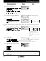
3-1
Enter the constants on the right side
of the equal sign into matrix C (3 x 1).
2nd F
8
MATRIX
B
3
3
ENTER
1
ENTER
1
ENTER
(-)
3
ENTER
ENTER
The system of equations can
be expressed as
1 2 1
2 1 -1
1 1 -2
x
y
z
=
8
1
-3
Let each matrix B, X, C :
BX = C
B-1BX = B-1C (multiply both
sides by B-1)
I = B-1 (B-1B = I, identity matrix)
X = B-1 C
3-2
Calculate B-1C.
2nd F
3-3
CL
2nd F
x -1
X
MATRIX
2nd F
A
2
MATRIX
A
3
ENTER
The 1 is the x coordinate, the 2
the y coordinate, and the 3 the
z coordinate of the solution
point.
(x, y, z)=(1, 2, 3)
Delete the input matrices for future
use.
2nd F OPTION
2
2nd F
C
ENTER
QUIT
○ ○ ○ ○ ○ ○ ○ ○ ○ ○ ○ ○ ○ ○ ○ ○ ○ ○ ○ ○ ○ ○ ○ ○ ○ ○ ○ ○ ○ ○ ○ ○ ○ ○ ○ ○ ○ ○ ○ ○ ○ ○ ○ ○ ○ ○ ○ ○ ○ ○ ○ ○ ○ ○ ○ ○ ○ ○ ○
The calculator can execute calculation of inverse matrix and matrix
multiplication. A system of linear equations can be solved easily using the
Matrix feature.
8-2
EL-9900 Graphing Calculator
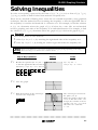
Solving Inequalities
To solve an inequality, expressed by the form of f (x) ≤ 0, f (x) ≥ 0, or form of f (x) ≤ g (x),
f (x) ≥ g (x), means to find all values that make the inequality true.
There are two methods of finding these values for one-variable inequalities, using graphical
techniques. The first method involves rewriting the inequality so that the right-hand side of
the inequality is 0 and the left-hand side is a function of x. For example, to find the solution
to f (x) < 0, determine where the graph of f (x) is below the x-axis. The second method
involves graphing each side of the inequality as an individual function. For example, to find
the solution to f (x) < g(x), determine where the graph of f (x) is below the graph of g (x).
Example
Solve an inequality in two methods.
1. Solve 3(4 - 2x) ≥ 5 - x, by rewriting the right-hand side of the inequality as 0.
2. Solve 3(4 - 2x) ≥ 5 - x, by shading the solution region that makes the inequality true.
Before There may be differences in the results of calculations and graph plotting depending on the setting.
Starting Return all settings to the default value and delete all data.
Step & Key Operation
1-1
1-2
Display
Rewrite the equation 3(4 - 2x) ≥ 5 - x
so that the right-hand side becomes 0,
and enter y = 3(4 - 2x) - 5 + x for Y1.
Y=
3
(
—
5
+
4
—
2
X/ /T/n
Notes
3(4 - 2x) ≥ 5 - x
➞ 3(4 - 2x) - 5 + x ≥ 0
)
X/ /T/n
View the graph.
GRAPH
1-3
Find the location of the x-intercept
and solve the inequality.
2nd F CALC
5
The x-intercept is located at
the point (1.4, 0).
Since the graph is above the
x-axis to the left of the x-intercept, the solution to the inequality 3(4 - 2x) - 5 + x ≥ 0 is
all values of x such that
x ≤ 1.4.
○ ○ ○ ○ ○ ○ ○ ○ ○ ○ ○ ○ ○ ○ ○ ○ ○ ○ ○ ○ ○ ○ ○ ○ ○ ○ ○ ○ ○ ○ ○ ○ ○ ○ ○ ○ ○ ○ ○ ○ ○ ○ ○ ○ ○ ○ ○ ○ ○ ○ ○ ○ ○ ○ ○ ○ ○ ○
9-1
EL-9900 Graphing Calculator
Step & Key Operation
2-1
Notes
Enter y = 3(4 - 2x) for Y1 and
y = 5 - x for Y2.
(7 times) DEL
Y=
ENTER
2-2
Display
5
(4 times)
X/ /T/n
—
View the graph.
GRAPH
2-3
Access the Set Shade screen.
2nd F DRAW
G
1
2-4
2-5
Set up the shading.
—F
2nd
VARS
A
2nd F
VARS
ENTER
ENTER
A
2
1
Since the inequality being
solved is Y1 ≥ Y2, the solution is where the graph of Y1
is “on the top” and Y2 is “on
the bottom.”
View the shaded region.
GRAPH
2-6
Find where the graphs intersect and
solve the inequality.
2nd F CALC
2
The point of intersection is
(1.4, 3.6). Since the shaded
region is to the left of x = 1.4,
the solution to the inequality
3(4 - 2x) ≥ 5 - x is all values
of x such that x ≤ 1.4.
○ ○ ○ ○ ○ ○ ○ ○ ○ ○ ○ ○ ○ ○ ○ ○ ○ ○ ○ ○ ○ ○ ○ ○ ○ ○ ○ ○ ○ ○ ○ ○ ○ ○ ○ ○ ○ ○ ○ ○ ○ ○ ○ ○ ○ ○ ○ ○ ○ ○ ○ ○ ○ ○ ○ ○ ○ ○
Graphical solution methods not only offer instructive visualization of the solution
process, but they can be applied to inequalities that are often difficult to solve
algebraically. The EL-9900 allows the solution region to be indicated visually using the
Shade feature. Also, the points of intersection can be obtained easily.
9-1
EL-9900 Graphing Calculator
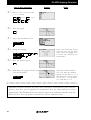
Solving Double Inequalities
The solution to a system of two inequalities in one variable consists of all values of the variable
that make each inequality in the system true. A system f (x) ≥ a, f (x) ≤ b, where the same expression
appears on both inequalities, is commonly referred to as a “double” inequality and is often written
in the form a ≤ f (x) ≤ b. Be certain that both inequality signs are pointing in the same direction and
that the double inequality is only used to indicate an expression in x “trapped” in between two
values. Also a must be less than or equal to b in the inequality a ≤ f (x) ≤ b or b ≥ f (x) ≥ a.
Example
Solve a double inequality, using graphical techniques.
2x - 5 ≥ -1
2x -5 ≤ 7
Before There may be differences in the results of calculations and graph plotting depending on the setting.
Starting Return all settings to the default value and delete all data.
Step & Key Operation
1
Enter y = -1 for Y1, y = 2x - 5 for
Y2, and y = 7 for Y3.
(-)
Y=
2
2
Display
X/ /T/n
1
—
Notes
The “double” inequality
given can also be written to
-1 ≤ 2x - 5 ≤ 7.
ENTER
5
ENTER
7
View the lines.
GRAPH
3
Find the point of intersection.
2nd F CALC
y = 2x - 5 and
y = -1 intersect at (2, -1).
2
9-2
EL-9900 Graphing Calculator
Step & Key Operation
4
Move the tracer and find another
intersection.
2nd F CALC
5
Display
Notes
y = 2x - 5 and y = 7
intersect at (6,7).
2
Solve the inequalities.
The solution to the “double”
inequality -1 ≤ 2x - 5 ≤ 7 consists of all values of x in between, and including, 2 and 6
(i.e., x ≥ 2 and x ≤ 6). The solution is 2 ≤ x ≤ 6.
○ ○ ○ ○ ○ ○ ○ ○ ○ ○ ○ ○ ○ ○ ○ ○ ○ ○ ○ ○ ○ ○ ○ ○ ○ ○ ○ ○ ○ ○ ○ ○ ○ ○ ○ ○ ○ ○ ○ ○ ○ ○ ○ ○ ○ ○ ○ ○ ○ ○ ○ ○ ○ ○ ○ ○ ○ ○
Graphical solution methods not only offer instructive visualization of the solution
process, but they can be applied to inequalities that are often difficult to solve
algebraically. The EL-9900 allows the solution region to be indicated visually using the
Shade feature. Also, the points of intersection can be obtained easily.
9-2
EL-9900 Graphing Calculator
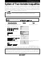
System of Two-Variable Inequalities
The solution region of a system of two-variable inequalities consists of all points (a, b) such
that when x = a and y = b, all inequalities in the system are true. To solve two-variable
inequalities, the inequalities must be manipulated to isolate the y variable and enter the
other side of the inequality as a function. The calculator will only accept functions of the
form y = . (where y is defined explicitly in terms of x).
Example
Solve a system of two-variable inequalities by shading the solution region.
2x + y ≥ 1
x2 + y ≤ 1
Before There may be differences in the results of calculations and graph plotting depending on the setting.
Starting Return all settings to the default value and delete all data.
Set the zoom to the decimal window: ZOOM
Step & Key Operation
Display
1
Rewrite each inequality in the system
so that the left-hand side is y :
2
Enter y = 1 - 2x for Y1 and y = 1 - x 2
for Y2.
Y=
1
3
1
—
—
2
X/ /T/n
x2
X/ /T/n
A ( ENTER 2nd F
) 7
Notes
2x + y ≥ 1 ➞ y ≥ 1 - 2x
x2 + y ≤ 1 ➞ y ≤ 1 - x2
ENTER
Access the set shade screen
2nd F DRAW
G
1
4
5
Shade the points of y -value so that
Y1 ≤ y ≤ Y2.
2nd F
VARS
A
2nd F
VARS
ENTER
ENTER
A
1
2
Graph the system and find the
intersections.
The intersections are (0, 1)
and (2, -3)
GRAPH
2nd F CALC
6
2
2nd F CALC
Solve the system.
2
The solution is 0 ≤ x ≤ 2.
○ ○ ○ ○ ○ ○ ○ ○ ○ ○ ○ ○ ○ ○ ○ ○ ○ ○ ○ ○ ○ ○ ○ ○ ○ ○ ○ ○ ○ ○ ○ ○ ○ ○ ○ ○ ○ ○ ○ ○ ○ ○ ○ ○ ○ ○ ○ ○ ○ ○ ○ ○ ○ ○ ○ ○ ○ ○
Graphical solution methods not only offer instructive visualization of the solution process,
but they can be applied to inequalities that are often difficult to solve algebraically.
The EL-9900 allows the solution region to be indicated visually using the Shade feature.
Also, the points of intersection can be obtained easily.
9-3
EL-9900 Graphing Calculator
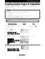
Graphing Solution Region of Inequalities
The solution region of an inequality consists of all points (a, b) such that when x = a, and y = b,
all inequalities are true.
Example
Check to see if given points are in the solution region of a system of inequalities.
1. Graph the solution region of a system of inequalities:
2.
x + 2y ≤ 1
x2 + y ≥ 4
Which of the following points are within the solution region?
(-1.6, 1.8), (-2, -5), (2.8, -1.4), (-8,4)
Before There may be differences in the results of calculations and graph plotting depending on the setting.
Starting Return all settings to the default value and delete all data.
Step & Key Operation
1-1
1-2
Rewrite the inequalities so that the
left-hand side is y.
a/b
2
X/ /T/n
—
4
ENTER
x2
Set the shade and view the solution
region.
2nd F DRAW
G
1
2nd F
A
ENTER
VARS
ENTER
A
2
1
GRAPH
Set the display area (window) to :
-9 < x < 3, -6 < y < 5.
WINDOW
ENTER
9-4
x + 2y ≤ 1 ➞ y ≤ 1-x
2
x 2+y ≥ 4 ➞ y ≥ 4 - x 2
X/ /T/n
—
1
2nd F VARS
GRAPH
2-1
Notes
Enter y = 1-x
for Y1 and
2
2
y = 4 - x for Y2.
Y=
1-3
Display
(-)
(-)
9
ENTER
6
ENTER
3
ENTER
5
ENTER
Y2 ≤ y ≤ Y1
EL-9900 Graphing Calculator
Step & Key Operation
2-2
Use the cursor to check the position
of each point. (Zoom in as necessary).
or
GRAPH
2-3
Display
or
or
Substitute points and confirm
whether they are in the solution
region.
(-)
2
X
1
1
•
•
6
8
...
+
(Continuing key operations omitted.)
Notes
Points in the solution region
are (2.8, -1.4) and (-8, 4).
Points outside the solution
region are (-1.6, 1.8) and
(-2, -5).
.(-1.6, 1.8): -1.6 + 2 1.8 = 2
➞ This does not materialize.
.(-2,
-5): -2 + 2 (-5) = -12
(-2) + (-5) = -1
➞ This does not materialize.
.(2.8, -1.4): 2.8 + 2 (-1.4) = 0
(2.8) + (-1.4) = 6.44
➞ This materializes.
.(-8, 4): -8 + 2 4 = 0
✕
✕
2
✕
2
✕
(-8)2 + 4 = 68
➞ This materializes.
○ ○ ○ ○ ○ ○ ○ ○ ○ ○ ○ ○ ○ ○ ○ ○ ○ ○ ○ ○ ○ ○ ○ ○ ○ ○ ○ ○ ○ ○ ○ ○ ○ ○ ○ ○ ○ ○ ○ ○ ○ ○ ○ ○ ○ ○ ○ ○ ○ ○ ○ ○ ○ ○ ○ ○ ○ ○ ○
Graphical solution methods not only offer instructive visualization of the solution process,
but they can be applied to inequalities that are often very difficult to solve algebraically.
The EL-9900 allows the solution region to be indicated visually using the Shading
feature. Also, the free-moving tracer or Zoom-in feature will allow the details to be
checked visually.
9-4
EL-9900 Graphing Calculator
Slope and Intercept of Absolute Value Functions
The absolute value of a real number x is defined by the following:
|x| =
x if x ≥ 0
-x if x ≤ 0
If n is a positive number, there are two solutions to the equation |f (x)| = n because there
are exactly two numbers with the absolute value equal to n: n and -n. The existence of two
distinct solutions is clear when the equation is solved graphically.
An absolute value function can be presented as y = a|x - h| + k. The graph moves as the
changes of slope a, x-intercept h, and y-intercept k.
Example
Consider various absolute value functions and check the relation between the
graphs and the values of coefficients.
1. Graph y = |x|
2. Graph y = |x -1| and y = |x|-1 using Rapid Graph feature.
Before There may be differences in the results of calculations and graph plotting depending on the setting.
Starting Return all settings to the default value and delete all data.
Set the zoom to the decimal window: ZOOM
Step & Key Operation
1-1
Display
) 7
Notes
Enter the function y =|x| for Y1.
Y=
1-2
A ( ENTER 2nd F
MATH
X/ /T/n
1
B
Notice that the domain of f(x)
= |x| is the set of all real numbers and the range is the set of
non-negative real numbers.
Notice also that the slope of the
graph is 1 in the range of X > 0
and -1 in the range of X ≤ 0.
View the graph.
GRAPH
○ ○ ○ ○ ○ ○ ○ ○ ○ ○ ○ ○ ○ ○ ○ ○ ○ ○ ○ ○ ○ ○ ○ ○ ○ ○ ○ ○ ○ ○ ○ ○ ○ ○ ○ ○ ○ ○ ○ ○ ○ ○ ○ ○ ○ ○ ○ ○ ○ ○ ○ ○ ○ ○ ○ ○ ○ ○
2-1
Enter the standard form of an absolute value function for Y2 using the
Rapid Graph feature.
Y=
X/ /T/n
2-2
A
ALPHA
H
MATH
B
+
1
ALPHA
Substitute the coefficients to graph
y = |x - 1|.
2nd F
0
10-1
—
ALPHA
SUB
ENTER
1
ENTER
1
ENTER
K
EL-9900 Graphing Calculator
Step & Key Operation
2-3
Display
View the graph.
Notice that placing an h (>0)
within the standard form
y = a|x - h|+ k will move the
graph right h units on the xaxis.
GRAPH
2-4
Change the coefficients to graph
y =|x|-1.
Y=
ENTER
2-5
Notes
2nd F
0
ENTER
View the graph.
GRAPH
SUB
(-)
ENTER
1
1
ENTER
Notice that adding a k (>0)
within the standard form
y=a|x-h|+k will move the
graph up k units on the y-axis.
The EL-9900 shows absolute values with | |, just as written on paper, by using the
Equation editor. Use of the calculator allows various absolute value functions to be
graphed quickly and shows their characteristics in an easy-to-understand manner.
10-1
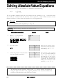
EL-9900 Graphing Calculator
Solving Absolute Value Equations
The absolute value of a real number x is defined by the following:
x if x ≥ 0
-x if x ≤ 0
|x| =
If n is a positive number, there are two solutions to the equation |f (x)| = n because there
are exactly two numbers with the absolute value equal to n: n and -n. The existence of two
distinct solutions is clear when the equation is solved graphically.
Example
Solve an absolute value equation |5 - 4x| = 6
Before There may be differences in the results of calculations and graph plotting depending on the setting.
Starting Return all settings to the default value and delete all data.
Step & Key Operation
1
X/ /T/n
MATH
1
B
5
—
4
6
ENTER
View the graph.
GRAPH
3
Notes
Enter y = |5 - 4x| for Y1.
Enter y = 6 for Y2.
Y=
2
Display
Find the points of intersection of
the two graphs and solve.
2nd F CALC
2
2nd F
2
CALC
There are two points of intersection of the absolute
value graph and the horizontal line y = 6.
The solution to the equation
|5 - 4x|= 6 consists of the two
values -0.25 and 2.75. Note
that although it is not as intuitively obvious, the solution
could also be obtained by
finding the x-intercepts of the
function y = |5x - 4| - 6.
○ ○ ○ ○ ○ ○ ○ ○ ○ ○ ○ ○ ○ ○ ○ ○ ○ ○ ○ ○ ○ ○ ○ ○ ○ ○ ○ ○ ○ ○ ○ ○ ○ ○ ○ ○ ○ ○ ○ ○ ○ ○ ○ ○ ○ ○ ○ ○ ○ ○ ○ ○ ○ ○ ○ ○ ○ ○
The EL-9900 shows absolute values with | |, just as written on paper, by
using the Equation editor. The graphing feature of the calculator shows the
solution of the absolute value function visually.
10-2
EL-9900 Graphing Calculator
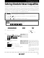
Solving Absolute Value Inequalities
To solve an inequality means to find all values that make the inequality true. Absolute value
inequalities are of the form |f (x)|< k, |f (x)|≤ k, |f (x)|> k, or |f (x)|≥ k. The graphical
solution to an absolute value inequality is found using the same methods as for normal
inequalities. The first method involves rewriting the inequality so that the right-hand side of
the inequality is 0 and the left-hand side is a function of x. The second method involves
graphing each side of the inequality as an individual function.
Example
Solve absolute value inequalities in two methods.
1. Solve
20 - 6x < 8 by rewriting the inequality so that the right-hand side of
5
the inequality is zero.
2. Solve
3.5x + 4 > 10 by shading the solution region.
Before There may be differences in the results of calculations and graph plotting depending on the setting.
Starting Return all settings to the default value and delete all data.
Set viewing window to “-5< x <50,” and “-10< y <10”.
WINDOW
(-)
5
ENTER
5
0
Step & Key Operation
1-1
1-2
Display
|20 -
Enter y = |20 - 6x | - 8 for Y1.
5
6
MATH
B
X/ /T/n
—
1
2
0
—
a/b
5
8
View the graph, and find the
x-intercepts.
GRAPH
CALC
5
➞ x = 10, y = 0
2nd F CALC
5
➞ x = 23.33333334
2nd F
y = 0.00000006 ( Note)
1-4
Notes
6x
|< 8
5
➞|20 - 6x | - 8 < 0.
5
Rewrite the equation.
Y=
1-3
ENTER
Solve the inequality.
The intersections with the xaxis are (10, 0) and (23.3, 0)
( Note: The value of y in the
x-intercepts may not appear
exactly as 0 as shown in the
example, due to an error
caused by approximate calculation.)
Since the graph is below the
x-axis for x in between the
two x-intercepts, the solution
is 10 < x < 23.3.
○ ○ ○ ○ ○ ○ ○ ○ ○ ○ ○ ○ ○ ○ ○ ○ ○ ○ ○ ○ ○ ○ ○ ○ ○ ○ ○ ○ ○ ○ ○ ○ ○ ○ ○ ○ ○ ○ ○ ○ ○ ○ ○ ○ ○ ○ ○ ○ ○ ○ ○ ○ ○ ○ ○ ○ ○ ○
10-3
EL-9900 Graphing Calculator
Step & Key Operation
2-1
2-3
3
•
1
0
CL
MATH
B
5
X/ /T/n
1
+
4
ENTER
Since the inequality you are
solving is Y1 > Y2, the solution is where the graph of Y2
is “on the bottom” and Y1 in
“on the top.”
Set up shading.
2nd F DRAW
G
1
2nd F
VARS
A
ENTER
2nd F
VARS
ENTER
A
2
1
Set viewing window to “-10 < x < 10”
and “-5 < y < 50”, and view the graph.
WINDOW
2-4
Notes
Enter the function
y =|3.5x + 4|for Y1.
Enter y = 10 for Y2.
Y=
2-2
Display
(-)
1
ENTER
ENTER
ENTER
5
0
ENTER
1
(-)
5
ENTER
0
5
0
ENTER
Find the points of intersection.
Solve the inequality.
CALC
2
➞ x = -4, y = 10
2nd F CALC
2
➞ x = 1.714285714
2nd F
y = 9.999999999 ( Note)
The intersections are (-4, 10)
and (1.7, 10.0). The solution
is all values of x such that
x <- 4 or x >1.7.
( Note: The value of y in the
intersection of the two graphs
may not appear exactly as 10
as shown in the example, due
to an error caused by approximate calculation.)
○ ○ ○ ○ ○ ○ ○ ○ ○ ○ ○ ○ ○ ○ ○ ○ ○ ○ ○ ○ ○ ○ ○ ○ ○ ○ ○ ○ ○ ○ ○ ○ ○ ○ ○ ○ ○ ○ ○ ○ ○ ○ ○ ○ ○ ○ ○ ○ ○ ○ ○ ○ ○ ○ ○ ○ ○ ○ ○
The EL-9900 shows absolute values with | |, just as written on paper, by using
the Equation editor. Graphical solution methods not only offer instructive
visualization of the solution process, but they can be applied to inequalities that
are often difficult to solve algebraically. The Shade feature is useful to solve the
inequality visually and the points of intersection can be obtained easily.
10-3
EL-9900 Graphing Calculator
Evaluating Absolute Value Functions
The absolute value of a real number x is defined by the following:
x if x ≥ 0
-x if x ≤ 0
Note that the effect of taking the absolute value of a number is to strip away the minus sign
if the number is negative and to leave the number unchanged if it is nonnegative.
Thus, |x|≥ 0 for all values of x.
Example
|x| =
Evaluate various absolute value functions.
1. Evaluate |- 2(5-1)|
2. Is |-2+7| = |-2| + |7|?
3.
Evaluate each side of the equation to check your answer.
Is |x + y| =|x|+ |y| for all real numbers x and y ?
If not, when will |x + y| = |x|+|y| ?
Is |6-9 | = |6-9| ?
1+3
|1+3|
Evaluate each side of the equation to check your answer. Investigate with
more examples, and decide if you think |x / y|=|x|/|y|
Before There may be differences in the results of calculations and graph plotting depending on the setting.
Starting Return all settings to the default value and delete all data.
Step & Key Operation
Display
1-1
Access the home or computation
screen.
1-2
Enter y = |-2(5-1)| and evaluate.
B
MATH
1
)
1
(-)
(
2
5
Notes
The solution is +8.
—
ENTER
○ ○ ○ ○ ○ ○ ○ ○ ○ ○ ○ ○ ○ ○ ○ ○ ○ ○ ○ ○ ○ ○ ○ ○ ○ ○ ○ ○ ○ ○ ○ ○ ○ ○ ○ ○ ○ ○ ○ ○ ○ ○ ○ ○ ○ ○ ○ ○ ○ ○ ○ ○ ○ ○ ○ ○ ○ ○
2-1
Evaluate|-2 + 7|. Evaluate|-2|+|7|.
➞|-2 + 7| ≠ |-2| + |7|.
CL
MATH
1
(-)
2
MATH
1
(-)
2
1
|-2 + 7| = 5, |-2| + |7| = 9
7
+
7
+
ENTER
MATH
ENTER
10-4
EL-9900 Graphing Calculator
Step & Key Operation
2-2
Display
Notes
Is |x + y| = |x| +|y|? Think about
this problem according to the cases
when x or y are positive or negative.
If x ≥ 0 and y ≥ 0
[e.g.; (x, y) = (2,7)]
|x +y| = |2 + 7| = 9
|x|+|y| = |2| + |7| = 9
If x ≤ 0 and y ≥ 0
[e.g.; (x, y) = (-2, 7)]
|x +y| = |-2 + 7| = 5
|x|+|y| = |-2| + |7| = 9
If x ≥ 0 and y ≤ 0
[e.g.; (x, y) = (2, -7)]
|x +y| = |2-7| = 5
|x|+|y| = |2| + |-7| = 9
If x ≤ 0 and y ≤ 0
[e.g.; (x, y) = (-2, -7)]
|x +y| = |-2-7| = 9
|x|+|y| = |-2| + |-7| = 9
➞|x + y| = |x| + |y|.
➞|x + y| ≠ |x| + |y|.
➞|x + y| ≠ |x| + |y|.
➞|x + y| = |x| + |y|.
Therefore |x +y|=|x|+|y|when x ≥ 0 and y ≥ 0,
and when x ≤ 0 and y ≤ 0.
○ ○ ○ ○ ○ ○ ○ ○ ○ ○ ○ ○ ○ ○ ○ ○ ○ ○ ○ ○ ○ ○ ○ ○ ○ ○ ○ ○ ○ ○ ○ ○ ○ ○ ○ ○ ○ ○ ○ ○ ○ ○ ○ ○ ○ ○ ○ ○ ○ ○ ○ ○ ○ ○ ○ ○ ○ ○
3-1
Evaluate 6-9 . Evaluate 6-9 .
1+3
1+3
CL
1
3-2
1
MATH
+
a/b
3
—
6
9
6-9
6-9
1+3 = 0.75 , 1+3 = 0 .75
➞
6-9
1+3
=
6-9
1+3
ENTER
MATH
1
6
—
9
MATH
1
1
+
3
a/b
ENTER
Is |x /y| = |x|/|y|?
Think about this problem according
to the cases when x or y are positive
or negative.
If x ≥ 0 and y ≥ 0
[e.g.; (x, y) = (2,7)]
|x /y| = |2/7| = 2/7
|x|/|y| = |2| /|7| = 2/7
If x ≤ 0 and y ≥ 0
[e.g.; (x, y) = (-2, 7)]
|x /y| = |(-2)/7| = 2/7
|x|/|y| = |-2| /|7| = 2/7
If x ≥ 0 and y ≤ 0
[e.g.; (x, y) = (2, -7)]
|x /y| = |2/(-7)| = 2/7
|x|/|y| = |2| /|-7| = 2/7
If x ≤ 0 and y ≤ 0
[e.g.; (x, y) = (-2, -7)]
|x /y| = |(-2)/-7| = 2/7
|x|/|y| = |-2| /|-7| = 2/7
➞|x /y| = |x| / |y|
➞|x /y| = |x| / |y|
➞|x /y| = |x| / |y|
➞|x /y| = |x| / |y|
The statement is true for all y ≠ 0.
○ ○ ○ ○ ○ ○ ○ ○ ○ ○ ○ ○ ○ ○ ○ ○ ○ ○ ○ ○ ○ ○ ○ ○ ○ ○ ○ ○ ○ ○ ○ ○ ○ ○ ○ ○ ○ ○ ○ ○ ○ ○ ○ ○ ○ ○ ○ ○ ○ ○ ○ ○ ○ ○ ○ ○ ○ ○ ○
The EL-9900 shows absolute values with | |, just as written on paper, by using
the Equation editor. The nature of arithmetic of the absolute value can be
learned through arithmetical operations of absolute value functions.
10-4
EL-9900 Graphing Calculator
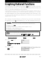
Graphing Rational Functions
p (x)
where p (x) and q (x) are two
q (x)
polynomial functions such that q (x) ≠ 0. The domain of any rational function consists of all
A rational function f (x) is defined as the quotient
values of x such that the denominator q (x) is not zero.
A rational function consists of branches separated by vertical asymptotes, and the values of
x that make the denominator q (x) = 0 but do not make the numerator p (x) = 0 are where
the vertical asymptotes occur. It also has horizontal asymptotes, lines of the form y = k (k,
a constant) such that the function gets arbitrarily close to, but does not cross, the horizontal
asymptote when |x| is large.
The x intercepts of a rational function f (x), if there are any, occur at the x-values that make
the numerator p (x), but not the denominator q (x), zero. The y-intercept occurs at f (0).
Example
Graph the rational function and check several points as indicated below.
x-1
Graph f (x) = x 2-1 .
Find the domain of f (x), and the vertical asymptote of f (x).
Find the x- and y-intercepts of f (x).
Estimate the horizontal asymptote of f (x).
1.
2.
3.
4.
Before There may be differences in the results of calculations and graph plotting depending on the setting.
Starting Return all settings to the default value and delete all data.
Set the zoom to the decimal window: ZOOM
Step & Key Operation
1-1
A ( ENTER
Display
ALPHA
)
7
Notes
Enter y = x2 - 1 for Y1.
x -1
Y=
a/b
—
1-2
X/ /T/n
—
X/ /T/n
x2
1
View the graph.
GRAPH
1
The function consists of two
branches separated by the vertical asymptote.
○ ○ ○ ○ ○ ○ ○ ○ ○ ○ ○ ○ ○ ○ ○ ○ ○ ○ ○ ○ ○ ○ ○ ○ ○ ○ ○ ○ ○ ○ ○ ○ ○ ○ ○ ○ ○ ○ ○ ○ ○ ○ ○ ○ ○ ○ ○ ○ ○ ○ ○ ○ ○ ○ ○ ○ ○ ○
11-1
EL-9900 Graphing Calculator
Step & Key Operation
2
Find the domain and the vertical
asymptote of f (x), tracing the
graph to find the hole at x = 1.
(repeatedly)
TRACE
Display
Notes
Since f (x) can be written as
x-1
, the domain
(x + 1)(x - 1)
consists of all real numbers x
such that x ≠ 1 and x ≠ -1.
There is no vertical asymptote
where x = 1 since this value
of x also makes the numerator zero. Next to the coordinates x = 0.9, y = 0.52, see that
the calculator does not display
a value for y at x = 1 since 1
is not in the domain of this
rational function.
○ ○ ○ ○ ○ ○ ○ ○ ○ ○ ○ ○ ○ ○ ○ ○ ○ ○ ○ ○ ○ ○ ○ ○ ○ ○ ○ ○ ○ ○ ○ ○ ○ ○ ○ ○ ○ ○ ○ ○ ○ ○ ○ ○ ○ ○ ○ ○ ○ ○ ○ ○ ○ ○ ○ ○ ○ ○ ○
3
Find the x- and y-intercepts of f (x).
2nd F
CALC
6
The y-intercept is at (0 ,1). Notice that there are no x-intercepts for the graph of f (x).
○ ○ ○ ○ ○ ○ ○ ○ ○ ○ ○ ○ ○ ○ ○ ○ ○ ○ ○ ○ ○ ○ ○ ○ ○ ○ ○ ○ ○ ○ ○ ○ ○ ○ ○ ○ ○ ○ ○ ○ ○ ○ ○ ○ ○ ○ ○ ○ ○ ○ ○ ○ ○ ○ ○ ○ ○ ○ ○
4
Estimate the horizontal asymptote
of f (x).
The line y = 0 is very likely a
horizontal asymptote of f (x).
○ ○ ○ ○ ○ ○ ○ ○ ○ ○ ○ ○ ○ ○ ○ ○ ○ ○ ○ ○ ○ ○ ○ ○ ○ ○ ○ ○ ○ ○ ○ ○ ○ ○ ○ ○ ○ ○ ○ ○ ○ ○ ○ ○ ○ ○ ○ ○ ○ ○ ○ ○ ○ ○ ○ ○ ○ ○ ○
The graphing feature of the EL-9900 can create the branches of a rational
function separated by a vertical asymptote. The calculator allows the points of
intersection to be obtained easily.
11-1
EL-9900 Graphing Calculator
Solving Rational Function Inequalities
p (x)
where p (x) and q (x) are two
q (x)
polynomial functions such that q (x) ≠ 0. The solutions to a rational function inequality can
A rational function f (x) is defined as the quotient
be obtained graphically using the same method as for normal inequalities. You can find the
solutions by graphing each side of the inequalities as an individual function.
Example
Solve a rational inequality.
x
Solve 1 - x 2 ≤ 2 by graphing each side of the inequality as an individual function.
Before There may be differences in the results of calculations and graph plotting depending on the setting.
Starting Return all settings to the default value and delete all data.
Set the zoom to the decimal window: ZOOM
Step & Key Operation
1
1
3
Display
ALPHA
) 7
Notes
x
Enter y =
for Y1. Enter y = 2
1- x 2
for Y2.
Y=
2
A ( ENTER
MATH
—
B
1
a/b
X/ /T/n
x2
ENTER
X/ /T/n
2
Set up the shading.
2nd F DRAW
G
1
2nd F
VARS
A
ENTER
2nd F
VARS
ENTER
A
1
Since Y1 is the value “on the
bottom” (the smaller of the
two) and Y2 is the function
“on the top” (the larger of the
two), Y1 < Y < Y2.
2
View the graph.
GRAPH
4
Find the intersections, and solve the
inequality.
2nd F CALC
2 Do this four times
The intersections are when
x = -1.3, -0.8, 0.8, and 1.3.
The solution is all values of
x such that x ≤ -1.3 or
-0.8 ≤ x ≤ 0.8 or x ≥ 1.3.
○ ○ ○ ○ ○ ○ ○ ○ ○ ○ ○ ○ ○ ○ ○ ○ ○ ○ ○ ○ ○ ○ ○ ○ ○ ○ ○ ○ ○ ○ ○ ○ ○ ○ ○ ○ ○ ○ ○ ○ ○ ○ ○ ○ ○ ○ ○ ○ ○ ○ ○ ○ ○ ○ ○ ○ ○ ○ ○
The EL-9900 allows the solution region of inequalities to be indicated visually
using the Shade feature. Also, the points of intersections can be obtained
easily.
11-2
EL-9900 Graphing Calculator
Graphing Parabolas
The graphs of quadratic equations (y = ax 2 + bx + c) are called parabolas. Sometimes the quadratic
equation takes on the form of x = ay 2 + by + c.
There is a problem entering this equation in the calculator graphing list for two reasons:
a) it is not a function, and only functions can be entered in the Y= list locations,
b) the functions entered in the Y= list must be in terms of x, not y.
There are, however, two methods you can use to draw the graph of a parabola.
Method 1: Consider the "top" and "bottom" halves of the parabola as two different parts of the graph
because each individually is a function. Solve the equation of the parabola for y and enter the two parts
(that individually are functions) in two locations of the Y= list.
Method 2: Choose the parametric graphing mode of the calculator and enter the parametric equations
of the parabola. It is not necessary to algebraically solve the equation for y. Parametric representations
are equation pairs x = F(t), y = F(t) that have x and y each expressed in terms of a third parameter, t.
Example
Graph a parabola using two methods.
1. Graph the parabola x = y
2. Graph the parabola x = y
2
-2 in rectangular mode.
2
-2 in parametric mode.
Before There may be differences in the results of calculations and graph plotting depending on the setting.
Starting Return all settings to the default value and delete all data.
Set the zoom to the decimal window: ZOOM
Step & Key Operation
Display
1-1
Solve the equation for y.
1-2
Enter y = √x+2 for Y1 and enter
y = -Y1 for Y2.
Y=
ENTER
1-3
2nd F
(-)
√
X/ /T/n
2nd F
View the graph.
GRAPH
VARS
+
A
A ( ENTER
ALPHA
) 7
Notes
x = y 2 -2
x + 2 = y2
y= +
–√ x + 2
2
ENTER
1
The graph of the equation y =
√x+ 2 is the "top half" of the
parabola and the graph of the
equation y = - √ x + 2 gives
the "bottom half."
○ ○ ○ ○ ○ ○ ○ ○ ○ ○ ○ ○ ○ ○ ○ ○ ○ ○ ○ ○ ○ ○ ○ ○ ○ ○ ○ ○ ○ ○ ○ ○ ○ ○ ○ ○ ○ ○ ○ ○ ○ ○ ○ ○ ○ ○ ○ ○ ○ ○ ○ ○ ○ ○ ○ ○ ○ ○ ○
12-1
EL-9900 Graphing Calculator
Step & Key Operation
2-1
Display
Notes
Change to parametric mode.
2nd F SET UP
E
2
2-2
Rewrite x = y 2 -2 in parametric form.
Enter X1T = T 2 -2 and Y1T = T.
Y=
X/ /T/n
x2
—
2
Let y = T and substitute in x
= y 2 - 2, to obtain x = T 2- 2.
ENTER
X/ /T/n
2-3
View the graph. Consider why only
half of the parabola is drawn.
(To understand this, use Trace feature.)
GRAPH
2-4
)
TRACE
Set Tmin to -6.
WINDOW
2-5
(
The graph starts at T =0 and
increases. Since the window
setting is T ≥ 0, the region T
< 0 is not drawn in the graph.
(-)
6
ENTER
View the complete parabola.
GRAPH
○ ○ ○ ○ ○ ○ ○ ○ ○ ○ ○ ○ ○ ○ ○ ○ ○ ○ ○ ○ ○ ○ ○ ○ ○ ○ ○ ○ ○ ○ ○ ○ ○ ○ ○ ○ ○ ○ ○ ○ ○ ○ ○ ○ ○ ○ ○ ○ ○ ○ ○ ○ ○ ○ ○ ○ ○ ○ ○
The calculator provides two methods for graphing parabolas, both of which
are easy to perform.
12-1
EL-9900 Graphing Calculator
Graphing Circles
The standard equation of a circle of radius r that is centered at a point (h, k) is (x - h) 2 +
(y - k) 2 = r 2. In order to put an equation in standard form so that you can graph in rectangular
mode, it is necessary to solve the equation for y. You therefore need to use the process of
completing the square.
Example
Graph the circles in rectangular mode. Solve the equation for y to put it in the
standard form.
1. Graph x
2. Graph x
2
+ y 2 = 4.
2
- 2x + y 2 + 4y = 2.
Before There may be differences in the results of calculations and graph plotting depending on the setting.
Starting Return all settings to the default value and delete all data.
Set the zoom to the decimal window: ZOOM
Step & Key Operation
1-1
ALPHA
Display
Solve the equation for y.
Enter y = √ 4 - x 2 for Y1 (the top
half). Enter y = -√ 4 - x 2 for Y2.
Y=
ENTER
1-2
A ( ENTER
2nd F
(-)
√
4
2nd F
X/ /T/n
—
VARS
A
) 7
Notes
y2 = 4 - x2
y= +
– √4 - x 2
x2
ENTER
1
This is a circle of radius r ,
centered at the origin.
View the graph.
GRAPH
○ ○ ○ ○ ○ ○ ○ ○ ○ ○ ○ ○ ○ ○ ○ ○ ○ ○ ○ ○ ○ ○ ○ ○ ○ ○ ○ ○ ○ ○ ○ ○ ○ ○ ○ ○ ○ ○ ○ ○ ○ ○ ○ ○ ○ ○ ○ ○ ○ ○ ○ ○ ○ ○ ○ ○ ○ ○
2-1
Solve the equation for y,
completing the square.
x 2 - 2x + y 2 + 4y = 2
Place all variable terms on the
left and the constant term on
the right-hand side of the
equation.
x 2 -2 x + y 2 +4 y + 4 = 2 + 4 Complete the square on the
y-term.
x 2 - 2x + (y+2)2 = 6
Express the terms in y as a
perfect square.
(y+2)2 = 6 -x 2 + 2x
Leave only the term involving
y on the left hand side.
y+2 = ±√6-x 2+2x
Take the square root of both
sides.
Solve for y.
y = ±√6-x 2+2x -2
12-2
EL-9900 Graphing Calculator
Step & Key Operation
2-2
Enter y = √6 - x 2 + 2x for Y1,
y = Y1 - 2 for Y2, and y = -Y1 -2 for
Y3.
Y=
x2
2nd F
2
(-)
2-3
Display
CL
+
VARS
√
6
—
X/ /T/n
ENTER
CL
2nd F
2
A
ENTER
X/ /T/n
ENTER
2nd F
VARS
ENTER
1
—
2
"Turn off" Y1 so that it will not
graph.
(3 times)
WINDOW
2
ENTER
—
2
Notice that “=” for Y1 is no
longer darkened. You now
have the top portion and the
bottom portion of the circle
in Y2 and Y3.
-1.3 < Y < 3.1
➝
Adjust the screen so that the whole
graph is shown. Shift 2 units downwards.
—
Notice that if you enter
y = √6 - x 2 + 2x - 2 for Y1
and y = - Y1 for Y2, you will
not get the graph of a circle
because the “±” does not go
with the “-2”.
—
1
ENTER
2-4
Notes
-5.1 < Y < 1.1
ENTER
GRAPH
○ ○ ○ ○ ○ ○ ○ ○ ○ ○ ○ ○ ○ ○ ○ ○ ○ ○ ○ ○ ○ ○ ○ ○ ○ ○ ○ ○ ○ ○ ○ ○ ○ ○ ○ ○ ○ ○ ○ ○ ○ ○ ○ ○ ○ ○ ○ ○ ○ ○ ○ ○ ○ ○ ○ ○ ○ ○ ○
Graphing circles can be performed easily on the calculator display.
12-2
EL-9900 Graphing Calculator
Graphing Ellipses
The standard equation for an ellipse whose center is at the point (h, k) with major and
2
2
minor axes of length a and b is (x -2 h) + (y -2 k) = 1.
a
b
There is a problem entering this equation in the calculator graphing list for two reasons:
a) it is not a function, and only functions can be entered in the Y = list locations.
b) the functions entered in the Y = list locations must be in terms of x, not y.
To draw a graph of an ellipse, consider the “top” and “bottom” halves of the ellipse as two
different parts of the graph because each individual is a function. Solve the equation of the
ellipse for y and enter the two parts in two locations of the Y = list.
Example
Graph an ellipse in rectangular mode. Solve the equation for y to put it in the
standard form.
Graph the ellipse 3(x -3) 2 + (y + 2) 2 = 3
Before There may be differences in the results of calculations and graph plotting depending on the setting.
Starting Return all settings to the default value and delete all data.
Set the zoom to the decimal window: ZOOM
Step & Key Operation
1
Display
Solve the equation for y, completing
the square.
Enter
Y1 = √3 - 3(x - 3)2
Y2 = Y1 - 2
Y3 = -Y1 -2
Y=
2nd F
X/ /T/n
—
2nd F
VARS
2
1
2
√
—
—
3
3
)
x2
ENTER
A
ENTER
(-)
ENTER
2nd F
VARS
—
ENTER
2
Turn off Y1 so that it will not graph.
ENTER
12-3
(
3
1
A ( ENTER
ALPHA
) 7
Notes
3(x - 3)2 + (y + 2)2 = 3
(y + 2)2 = 3 - 3(x - 3)2
y + 2 = +√3 - 3(x - 3)2
y = + √3 - 3(x - 3)2 - 2
EL-9900 Graphing Calculator
Step & Key Operation
3
Display
Notes
View the graph.
GRAPH
4
(3 times)
WINDOW
—
2
ENTER
—
2
-3.1 < Y < 3.1
➝
Adjust the screen so that the whole
graph is shown. Shift 2 units downwards.
-5.1 < Y < 1.1
ENTER
GRAPH
○ ○ ○ ○ ○ ○ ○ ○ ○ ○ ○ ○ ○ ○ ○ ○ ○ ○ ○ ○ ○ ○ ○ ○ ○ ○ ○ ○ ○ ○ ○ ○ ○ ○ ○ ○ ○ ○ ○ ○ ○ ○ ○ ○ ○ ○ ○ ○ ○ ○ ○ ○ ○ ○ ○ ○ ○ ○ ○
Graphing an ellipse can be performed easily on the calculator display.
12-3
EL-9900 Graphing Calculator
Graphing Hyperbolas
The standard equation for a hyperbola can take one of two forms:
( x - h ) 2 - ( y - k ) 2 = 1 with vertices at ( h ± a, k ) or
a2
b2
2
( x - k ) - ( y - h) 2 = 1 with vertices at ( h, k ± b ).
a2
b2
There is a problem entering this equation in the calculator graphing list for two reasons:
a) it is not a function, and only functions can be entered in the Y= list locations.
b) the functions entered in the Y= list locations must be in terms of x, not y.
To draw a graph of a hyperbola, consider the “top” and “bottom” halves of the hyperbola
as two different parts of the graph because each individual is a function. Solve the equation
of the hyperbola for y and enter the two parts in two locations of the Y= list.
Example
Graph a hyperbola in rectangular mode. Solve the equation for y to put it in the
standard form.
Graph the hyperbola x 2 + 2x - y 2 - 6y + 3 = 0
Before There may be differences in the results of calculations and graph plotting depending on the setting.
Starting Return all settings to the default value and delete all data.
Set the zoom to the decimal window: ZOOM
Step & Key Operation
1
Display
Solve the equation for y completing
the square.
Y1 = √x 2 + 2x + 12
Y2 = Y1 -3
Y3 = -Y1 -3
2
√
2nd F
X/ /T/n
+
1
2nd F
VARS
A
(-)
2nd F
VARS
x2
X/ /T/n
2
2
—
3
ENTER
ENTER
1
A
ENTER
1
ENTER
—
Turn off Y1 so that it will not graph.
ENTER
12-4
+
ALPHA
) 7
Notes
x 2 + 2x - y 2 -6y = -3
x 2 + 2x - (y 2 + 6y + 9) = -3 -9
x 2 + 2x - (y +3)2 = -12
(y + 3)2 = x 2 + 2x + 12
y + 3 = + √x 2 + 2x + 12
y = + √x 2 + 2x + 12 - 3
Enter
Y=
A ( ENTER
3
EL-9900 Graphing Calculator
Step & Key Operation
3
Display
Notes
View the graph.
GRAPH
4
Zoom out the screen.
ZOOM
A
4
○ ○ ○ ○ ○ ○ ○ ○ ○ ○ ○ ○ ○ ○ ○ ○ ○ ○ ○ ○ ○ ○ ○ ○ ○ ○ ○ ○ ○ ○ ○ ○ ○ ○ ○ ○ ○ ○ ○ ○ ○ ○ ○ ○ ○ ○ ○ ○ ○ ○ ○ ○ ○ ○ ○ ○ ○ ○ ○
Graphing hyperbolas can be performed easily on the calculator display.
12-4
Key pad for the SHARP EL-9900 Calculator
Advanced Keyboard
Graphing keys
Cursor movement keys
Power supply ON/OFF key
Clear/Quit key
Secondary function specification key
Variable enter key
Alphabet specification key
Calculation execute key
Display screen
Communication port for peripheral devices
Key pad for the SHARP EL-9900 Calculator
Basic Keyboard
Graphing keys
Cursor movement keys
Power supply ON/OFF key
Clear/Quit key
Secondary function specification key
Variable enter key
Alphabet specification key
Calculation execute key
Display screen
Communication port for peripheral devices
○
○
○
○
○
○
○
○
○
○
○
Dear Sir/Madam
We would like to take this opportunity to invite you to create a mathematical problem which can be solved
with the SHARP graphing calculator EL-9900. For this purpose, we would be grateful if you would complete the form below and return it to us by fax or mail.
If your contribution is chosen, your name will be included in the next edition of The EL-9900 Graphing
Calculator Handbook. We regret that we are unable to return contributions.
We thank you for your cooperation in this project.
○
○
○
○
○
○
○
○
○
○
○
○
○
○
○
○
○
○
○
○
○
○
○
○
Use this form to send us your contribution
Ms. )
Mr.
○
○
○
Name: (
○
○
○
School/College/Univ.:
○
○
Address:
Country:
○
○
○
Post Code:
Fax:
○
○
Phone:
SUBJECT : Write a title or the subject you are writing about.
○
○
○
○
○
○
○
○
○
○
○
○
○
○
○
○
○
○
○
○
○
○
○
○
○
○
○
○
○
○
○
○
○
○
○
○
○
○
○
○
○
○
○
○
○
○
○
○
○
○
○
○
○
○
○
○
○
○
○
INTRODUCTION : Write an explanation about the subject.
○
○
○
○
○
○
○
○
○
○
○
○
○
○
○
E-mail:
○
○
○
○
○
○
○
○
○
○
○
○
○
○
○
○
○
○
○
○
○
○
○
○
○
○
○
○
○
○
○
○
○
○
○
○
○
○
○
○
○
○
○
○
○
○
○
○
○
○
○
○
○
○
○
○
○
○
○
○
○
○
○
○
○
○
○
○
○
○
○
○
○
○
○
○
○
○
○
○
○
○
○
○
○
○
○
○
○
○
○
○
○
○
○
○
○
○
○
○
○
○
○
○
○
○
○
○
○
○
○
○
○
○
○
○
○
○
○
○
○
○
○
○
○
○
○
○
○
○
○
○
○
○
○
○
○
○
○
○
○
○
○
○
○
○
○
○
○
○
○
○
○
○
○
○
○
○
○
○
○
○
○
○
○
○
○
○
○
○
○
○
○
○
○
○
○
○
○
○
○
○
○
○
○
○
○
○
○
○
○
○
○
○
○
○
○
○
○
○
○
○
○
○
○
○
○
○
○
○
○
○
○
○
○
○
○
○
○
○
○
○
○
○
○
○
○
○
○
○
○
○
○
○
○
○
○
○
○
○
○
○
○
○
○
○
○
○
○
○
○
○
○
○
○
○
○
○
○
○
○
○
○
○
○
○
○
○
○
○
○
○
○
○
○
○
○
○
○
○
○
○
○
○
○
○
○
○
○
○
○
○
○
○
EXAMPLE : Write example problems.
○
○
○
○
○
○
○
○
○
○
○
○
○
○
○
○
○
○
○
○
○
○
○
○
○
○
○
○
○
○
○
○
○
○
○
○
○
○
○
○
○
○
○
○
○
○
○
○
○
○
○
○
○
○
○
○
○
○
○
○
○
○
○
○
○
○
○
○
○
○
○
○
○
○
○
○
○
○
○
○
○
○
○
○
○
○
○
○
○
○
○
○
○
○
○
○
○
○
○
○
○
○
○
○
○
○
○
○
○
○
○
○
○
○
○
○
○
○
○
○
○
○
○
○
○
○
○
○
○
○
○
○
○
○
○
○
○
○
○
○
○
○
○
○
○
○
○
○
○
○
○
○
○
○
○
○
○
○
○
○
○
○
○
○
○
○
○
○
○
○
○
○
○
○
○
○
○
○
○
○
○
○
○
○
○
○
○
○
○
○
○
○
○
○
○
○
○
○
○
○
○
○
○
○
○
○
○
○
○
○
○
○
○
○
○
○
○
○
○
○
○
○
○
○
○
○
○
○
○
○
○
○
○
○
○
○
○
○
○
○
○
○
○
○
○
○
○
○
○
○
○
○
○
○
○
○
○
○
○
○
○
○
○
○
○
○
○
○
○
○
○
○
○
○
○
○
○
○
○
○
○
○
○
○
○
○
○
○
○
○
○
○
○
○
○
○
○
○
○
○
○
○
○
○
○
○
○
○
○
○
○
○
○
○
○
○
○
○
○
○
○
○
○
○
○
○
○
○
○
○
○
○
○
○
○
○
○
○
○
○
○
○
○
○
○
○
○
○
○
○
○
○
○
○
○
○
○
○
○
○
○
○
○
○
○
○
○
○
○
○
○
○
○
○
○
○
○
○
○
○
○
○
○
○
○
○
○
○
○
○
○
○
○
○
○
○
○
○
SHARP Graphing Calculator
○
○
○
○
○
○
○
○
○
○
○
○
○
BEFORE STARTING : Write any conditions to be set up before solving the problems.
○
○
○
○
○
○
○
○
○
○
○
○
○
○
○
○
○
○
○
○
○
○
○
○
○
○
○
○
○
○
○
○
○
○
○
○
○
○
○
○
○
○
○
○
○
○
○
○
○
○
○
○
○
○
○
○
○
○
○
○
○
○
○
○
○
○
○
○
○
○
○
○
○
○
○
○
○
○
○
○
○
○
○
○
○
○
○
○
○
○
○
○
○
○
○
○
○
○
○
○
○
○
○
○
○
○
○
○
○
○
○
○
○
○
○
○
○
○
○
○
○
○
○
○
○
○
○
○
○
○
○
○
○
○
○
○
○
○
○
○
○
○
○
○
○
○
○
○
○
○
○
○
○
○
○
○
○
○
○
○
○
○
○
○
○
○
○
○
○
○
○
○
○
○
○
○
○
○
○
○
○
○
○
○
○
○
○
○
NOTES
○
○
○
○
○
○
○
○
○
○
○
○
○
○
○
○
○
○
○
○
○
○
○
○
○
○
○
○
○
○
○
○
○
○
○
○
○
○
○
○
○
○
○
○
○
○
○
○
○
○
○
○
○
○
○
○
○
○
○
○
○
○
○
○
○
○
○
○
○
○
○
○
○
○
○
○
○
○
○
○
○
○
○
○
○
○
○
○
○
○
○
○
○
○
○
○
○
○
○
○
○
○
○
○
○
○
○
○
○
○
○
○
○
○
○
○
○
○
○
○
○
○
○
○
○
○
○
○
○
○
○
○
○
○
○
○
○
○
○
○
○
○
○
○
○
○
○
○
○
○
○
○
○
○
○
○
○
○
○
○
○
○
○
○
○
○
○
○
○
○
○
○
○
○
○
○
○
○
○
○
○
○
○
○
○
○
○
○
○
○
○
○
○
○
○
○
○
○
○
○
○
○
○
○
○
○
○
○
○
○
○
○
○
○
○
○
○
○
○
○
○
○
○
○
○
○
○
○
○
○
○
○
○
○
○
○
○
○
○
○
○
○
○
○
○
○
○
○
○
○
○
○
○
○
○
○
○
○
○
○
○
○
○
○
○
○
○
○
○
○
○
○
○
○
○
○
○
○
○
○
○
○
○
○
○
○
○
○
○
○
○
○
○
○
○
○
○
○
○
○
○
○
○
○
○
○
○
○
○
○
○
○
○
○
○
○
○
○
○
○
○
○
○
○
○
○
○
○
○
○
○
○
○
○
○
○
○
○
○
○
○
○
○
○
○
○
○
○
○
○
○
○
○
○
○
○
○
○
○
○
○
○
○
○
○
○
○
○
○
○
○
○
○
○
○
○
○
○
○
○
○
○
○
○
○
○
○
○
○
○
○
○
○
○
○
○
○
○
○
○
○
○
○
○
○
○
○
○
○
○
○
○
○
○
○
○
○
○
○
○
○
○
○
○
○
○
○
○
○
○
○
○
○
○
○
○
○
○
○
○
○
○
○
○
○
○
○
○
○
○
○
○
○
○
○
○
○
○
○
○
○
○
○
○
○
○
○
○
○
○
○
○
○
○
○
○
○
○
○
○
○
○
○
○
○
○
○
○
○
○
○
○
○
○
○
○
○
○
○
○
○
○
○
○
○
○
○
○
○
○
○
○
○
○
○
○
○
○
○
○
○
○
○
○
○
○
○
○
○
○
○
○
○
○
○
○
○
○
○
○
○
○
○
○
○
○
○
○
○
○
○
○
○
○
○
○
○
○
○
○
○
○
○
○
○
○
○
○
○
○
○
○
○
○
○
○
○
○
○
○
○
○
○
○
○
○
○
○
○
○
○
○
○
○
○
○
○
○
○
○
○
○
○
○
○
○
○
○
○
○
○
○
○
○
○
○
○
○
○
○
○
○
○
○
○
○
○
○
○
○
○
○
○
○
○
○
○
○
○
○
○
○
○
○
○
○
○
○
○
○
○
○
○
○
○
○
○
○
○
○
○
○
○
○
○
○
○
○
○
○
○
○
○
○
○
○
○
○
○
○
○
○
○
○
○
○
○
○
○
○
○
○
○
○
○
○
○
○
○
○
○
○
○
○
○
○
○
○
○
○
○
○
○
○
○
○
○
○
○
○
○
○
○
○
○
○
○
○
○
○
○
○
○
○
○
○
○
○
○
○
○
○
○
○
○
○
○
○
○
○
○
○
○
○
○
○
○
○
○
○
○
○
○
○
○
○
○
○
○
○
○
○
○
○
○
○
○
○
○
○
○
○
○
○
○
○
○
○
○
○
○
○
○
○
○
○
○
○
○
○
○
○
○
○
○
○
○
○
○
○
○
○
○
○
○
○
○
○
○
○
○
○
○
○
○
○
○
○
○
○
○
○
○
○
○
○
○
○
○
○
○
○
○
○
○
○
○
○
○
○
○
○
○
○
○
○
○
○
○
○
○
○
○
○
○
○
○
○
○
○
○
○
○
○
○
○
○
○
○
○
○
○
○
○
○
○
○
○
○
○
○
○
○
○
○
○
○
○
○
○
○
○
○
○
○
○
○
○
○
○
○
○
○
○
○
○
○
○
○
○
○
○
○
○
○
○
○
○
○
○
○
○
○
○
○
○
○
○
○
○
○
○
○
○
○
○
○
○
○
○
○
○
○
○
○
○
○
○
○
○
○
○
○
○
○
○
○
○
○
○
○
○
○
○
○
○
○
○
○
○
○
○
○
○
○
○
○
○
○
○
○
○
○
○
○
○
○
○
○
○
○
○
○
○
○
○
○
○
○
○
○
○
○
○
○
○
○
○
○
○
○
○
○
○
○
○
○
○
○
○
○
○
○
○
○
○
○
○
○
○
○
○
○
○
○
○
○
○
○
○
○
○
○
○
○
○
○
○
○
○
○
○
○
○
○
○
○
○
○
○
○
○
○
○
○
○
○
○
○
○
○
○
○
○
○
○
○
○
○
○
○
○
○
○
○
○
○
○
○
○
○
○
○
○
○
○
○
○
○
○
○
○
○
○
○
○
○
○
○
○
○
○
○
○
○
○
○
○
○
○
○
○
○
○
○
○
○
○
○
○
○
○
○
○
○
○
○
○
○
○
○
○
○
○
○
○
○
○
○
○
○
○
○
○
○
○
○
○
○
○
○
○
○
○
○
○
○
○
○
○
○
○
○
○
○
○
○
○
○
○
○
○
○
○
○
○
○
○
○
○
○
○
○
○
○
○
○
○
○
○
○
○
○
○
○
○
○
○
○
○
○
○
○
○
○
○
○
○
○
○
○
○
○
○
○
○
○
○
○
○
○
○
○
○
○
○
○
○
○
○
○
○
○
○
○
○
○
○
○
○
○
○
○
○
○
○
○
○
○
○
○
○
○
○
○
○
○
○
○
○
○
○
○
○
○
○
○
○
○
○
○
○
○
○
○
○
○
○
○
○
○
○
○
○
○
○
○
○
○
○
○
○
○
○
○
○
○
○
○
○
○
○
○
○
○
○
○
○
○
○
○
○
○
○
○
○
○
○
○
○
○
○
○
○
○
○
○
○
○
○
○
○
○
○
○
○
SHARP CORPORATION Osaka, Japan
○
○
○
○
○
○
○
○
SHARP Graphing Calculator
○
○
○
○
○
○
○
○
○
○
Fax:
○
○
○
○
○
○
○
○
○
○
○
○
○
○
○
○
○
○
○
○
○
○
○
○
○
○
○
○
○
○
○
○
○
○
○
○
○
○
○
○
○
○
○
○
○
○
○
○
○
○
○
○
○
○
○
○
○
○
○
○
○
○
○
○
○
STEP
SHARP CORPORATION OSAKA, JAPAN