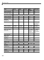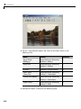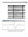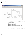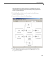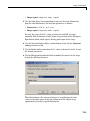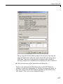
1
Video and Image Processing Blockset 2
User’s Guide
How to Contact The MathWorks
Web
Newsgroup
www.mathworks.com/contact_TS.html Technical Support
www.mathworks.com
comp.soft-sys.matlab
[email protected]
[email protected]
[email protected]
[email protected]
[email protected]
Product enhancement suggestions
Bug reports
Documentation error reports
Order status, license renewals, passcodes
Sales, pricing, and general information
508-647-7000 (Phone)
508-647-7001 (Fax)
The MathWorks, Inc.
3 Apple Hill Drive
Natick, MA 01760-2098
For contact information about worldwide offices, see the MathWorks Web site.
Video and Image Processing Blockset User’s Guide
© COPYRIGHT 2004–2007 by The MathWorks, Inc.
The software described in this document is furnished under a license agreement. The software may be used
or copied only under the terms of the license agreement. No part of this manual may be photocopied or
reproduced in any form without prior written consent from The MathWorks, Inc.
FEDERAL ACQUISITION: This provision applies to all acquisitions of the Program and Documentation
by, for, or through the federal government of the United States. By accepting delivery of the Program or
Documentation, the government hereby agrees that this software or documentation qualifies as commercial
computer software or commercial computer software documentation as such terms are used or defined
in FAR 12.212, DFARS Part 227.72, and DFARS 252.227-7014. Accordingly, the terms and conditions of
this Agreement and only those rights specified in this Agreement, shall pertain to and govern the use,
modification, reproduction, release, performance, display, and disclosure of the Program and Documentation
by the federal government (or other entity acquiring for or through the federal government) and shall
supersede any conflicting contractual terms or conditions. If this License fails to meet the government’s
needs or is inconsistent in any respect with federal procurement law, the government agrees to return the
Program and Documentation, unused, to The MathWorks, Inc.
Trademarks
MATLAB, Simulink, Stateflow, Handle Graphics, Real-Time Workshop, and xPC TargetBox
are registered trademarks, and SimBiology, SimEvents, and SimHydraulics are trademarks of
The MathWorks, Inc.
Other product or brand names are trademarks or registered trademarks of their respective
holders.
Patents
The MathWorks products are protected by one or more U.S. patents. Please see
www.mathworks.com/patents for more information.
Revision History
July 2004
October 2004
March 2005
September 2005
November 2005
March 2006
September 2006
March 2007
First printing
Second printing
Online only
Online only
Online only
Online only
Online only
Online only
New for Version 1.0 (Release 14)
Revised for Version 1.0.1 (Release 14SP1)
Revised for Version 1.1 (Release 14SP2)
Revised for Version 1.2 (Release 14SP3)
Revised for Version 2.0 (Release 14SP3+)
Revised for Version 2.1 (Release 2006a)
Revised for Version 2.2 (Release 2006b)
Revised for Version 2.3 (Release 2007a)
Contents
Getting Started
1
What Is Video and Image Processing Blockset? . . . . . . .
1-2
Installation . . . . . . . . . . . . . . . . . . . . . . . . . . . . . . . . . . . . . . .
Installing Video and Image Processing Blockset . . . . . . . . .
Required Products . . . . . . . . . . . . . . . . . . . . . . . . . . . . . . . . .
Related Products . . . . . . . . . . . . . . . . . . . . . . . . . . . . . . . . . .
1-3
1-3
1-4
1-4
Product Demos . . . . . . . . . . . . . . . . . . . . . . . . . . . . . . . . . . . .
Demos in the Help Browser . . . . . . . . . . . . . . . . . . . . . . . . .
Demos on the Web . . . . . . . . . . . . . . . . . . . . . . . . . . . . . . . . .
Demos on MATLAB Central . . . . . . . . . . . . . . . . . . . . . . . . .
1-5
1-5
1-6
1-6
Working with the Documentation . . . . . . . . . . . . . . . . . . .
Viewing the Documentation . . . . . . . . . . . . . . . . . . . . . . . . .
Printing the Documentation . . . . . . . . . . . . . . . . . . . . . . . . .
Using This Guide . . . . . . . . . . . . . . . . . . . . . . . . . . . . . . . . .
1-7
1-7
1-8
1-8
Key Blockset Concepts . . . . . . . . . . . . . . . . . . . . . . . . . . . . .
Image Types . . . . . . . . . . . . . . . . . . . . . . . . . . . . . . . . . . . . .
Video in Video and Image Processing Blockset . . . . . . . . . .
Defining Intensity and Color . . . . . . . . . . . . . . . . . . . . . . . .
Color Image Processing . . . . . . . . . . . . . . . . . . . . . . . . . . . . .
Coordinate Systems . . . . . . . . . . . . . . . . . . . . . . . . . . . . . . .
Image Data Stored in Column-Major Format . . . . . . . . . . .
Sample Time . . . . . . . . . . . . . . . . . . . . . . . . . . . . . . . . . . . . .
Video Duration and Simulation Time . . . . . . . . . . . . . . . . .
Normal and Accelerator Mode . . . . . . . . . . . . . . . . . . . . . . .
Strategies for Real-Time Video Processing . . . . . . . . . . . . .
Code Generation . . . . . . . . . . . . . . . . . . . . . . . . . . . . . . . . . .
1-11
1-12
1-12
1-13
1-14
1-19
1-21
1-21
1-22
1-23
1-24
1-26
Block Data Type Support . . . . . . . . . . . . . . . . . . . . . . . . . . .
1-28
Image Credits . . . . . . . . . . . . . . . . . . . . . . . . . . . . . . . . . . . . .
1-32
v
Importing and Exporting Video
2
Working with AVI Files . . . . . . . . . . . . . . . . . . . . . . . . . . . . .
Importing and Viewing AVI Files . . . . . . . . . . . . . . . . . . . . .
Exporting to AVI Files . . . . . . . . . . . . . . . . . . . . . . . . . . . . .
Annotating AVI Files with Video Frame Numbers . . . . . . .
Annotating AVI Files at Two Separate Locations . . . . . . . .
Saving Portions of an AVI File to Separate Files . . . . . . . .
2-2
2-2
2-6
2-9
2-13
2-18
Working with Multimedia Files . . . . . . . . . . . . . . . . . . . . .
Importing and Viewing Multimedia Files . . . . . . . . . . . . . .
Exporting to Multimedia Files . . . . . . . . . . . . . . . . . . . . . . .
Working with Audio . . . . . . . . . . . . . . . . . . . . . . . . . . . . . . .
2-25
2-25
2-27
2-31
Working with MPlay
3
Viewing Videos from the MATLAB Workspace . . . . . . . .
3-2
Viewing Video Files . . . . . . . . . . . . . . . . . . . . . . . . . . . . . . . .
3-6
Viewing Video Signals in Simulink . . . . . . . . . . . . . . . . . .
3-8
Conversions
4
vi
Contents
Intensity to Binary Conversion . . . . . . . . . . . . . . . . . . . . .
Thresholding Intensity Images Using Relational
Operators . . . . . . . . . . . . . . . . . . . . . . . . . . . . . . . . . . . . . .
Thresholding Intensity Images Using the Autothreshold
Block . . . . . . . . . . . . . . . . . . . . . . . . . . . . . . . . . . . . . . . . .
4-2
Color Space Conversion . . . . . . . . . . . . . . . . . . . . . . . . . . . .
Converting Color Information from R’G’B’ to Intensity . . .
4-14
4-14
4-2
4-7
Chroma Resampling . . . . . . . . . . . . . . . . . . . . . . . . . . . . . . .
4-19
Geometric Transformation
5
Interpolation Overview . . . . . . . . . . . . . . . . . . . . . . . . . . . .
Nearest Neighbor Interpolation . . . . . . . . . . . . . . . . . . . . . .
Bilinear Interpolation . . . . . . . . . . . . . . . . . . . . . . . . . . . . . .
Bicubic Interpolation . . . . . . . . . . . . . . . . . . . . . . . . . . . . . .
5-2
5-2
5-3
5-4
Rotating an Image . . . . . . . . . . . . . . . . . . . . . . . . . . . . . . . . .
5-6
Resizing an Image . . . . . . . . . . . . . . . . . . . . . . . . . . . . . . . . .
5-13
Cropping an Image . . . . . . . . . . . . . . . . . . . . . . . . . . . . . . . .
5-20
Morphological Operations
6
Overview of Morphology . . . . . . . . . . . . . . . . . . . . . . . . . . .
6-2
......................
6-3
Correcting for Nonuniform Illumination . . . . . . . . . . . . .
6-11
Counting Objects in an Image
Analysis and Enhancement
7
Feature Extraction . . . . . . . . . . . . . . . . . . . . . . . . . . . . . . . .
Finding Edges in Images . . . . . . . . . . . . . . . . . . . . . . . . . . .
Finding Lines in Images . . . . . . . . . . . . . . . . . . . . . . . . . . . .
Measuring an Angle Between Lines . . . . . . . . . . . . . . . . . .
7-2
7-2
7-9
7-17
vii
Image Enhancement . . . . . . . . . . . . . . . . . . . . . . . . . . . . . . .
Sharpening and Blurring an Image . . . . . . . . . . . . . . . . . . .
Removing Salt and Pepper Noise from Images . . . . . . . . . .
Removing Periodic Noise from Video . . . . . . . . . . . . . . . . . .
Adjusting the Contrast in Intensity Images . . . . . . . . . . . .
Adjusting the Contrast in Color Images . . . . . . . . . . . . . . .
7-27
7-27
7-35
7-41
7-48
7-53
Pixel Statistics . . . . . . . . . . . . . . . . . . . . . . . . . . . . . . . . . . . .
Finding the Histogram of an Image . . . . . . . . . . . . . . . . . . .
7-59
7-59
Example Applications
8
Pattern Matching . . . . . . . . . . . . . . . . . . . . . . . . . . . . . . . . . .
Tracking an Object Using Correlation . . . . . . . . . . . . . . . . .
8-2
8-2
Motion Compensation . . . . . . . . . . . . . . . . . . . . . . . . . . . . . .
8-9
Image Compression . . . . . . . . . . . . . . . . . . . . . . . . . . . . . . . .
Compressing an Image . . . . . . . . . . . . . . . . . . . . . . . . . . . . .
Viewing the Compressed Image . . . . . . . . . . . . . . . . . . . . . .
8-11
8-11
8-18
Index
viii
Contents
1
Getting Started
Video and Image Processing Blockset is a tool for processing images and
video in the Simulink® environment. This chapter provides an introduction
to Video and Image Processing Blockset, its product requirements, and its
documentation.
What Is Video and Image Processing
Blockset? (p. 1-2)
Learn more about Video and
Image Processing Blockset and its
components.
Installation (p. 1-3)
Install Video and Image Processing
Blockset and learn about the
products required to run the models
in this manual.
Product Demos (p. 1-5)
View the demos available in the
product and on the Web.
Working with the Documentation
(p. 1-7)
Learn how to view and print the
documentation.
Key Blockset Concepts (p. 1-11)
Understand how your image and
video data is interpreted within the
Simulink environment.
Block Data Type Support (p. 1-28)
Learn which data types are
supported by each Video and Image
Processing Blockset block.
Image Credits (p. 1-32)
View a list of the copyright owners
of the images used in the Video
and Image Processing Blockset
documentation.
1
Getting Started
What Is Video and Image Processing Blockset?
Video and Image Processing Blockset is a tool used for the rapid design,
prototyping, graphical simulation, and efficient code generation of video
processing algorithms. Video and Image Processing Blockset blocks can import
streaming video into the Simulink environment and perform two-dimensional
filtering, geometric and frequency transforms, block processing, motion
estimation, edge detection and other signal processing algorithms. You
can also use the blockset in conjunction with Real-Time Workshop® to
automatically generate embeddable C code for real-time execution.
Video and Image Processing Blockset blocks support floating-point, integer,
and fixed-point data types. To use any data type other than double-precision
and single-precision floating point, you must install Simulink Fixed Point.
For more information about this product, see the Simulink Fixed Point
documentation.
1-2
Installation
Installation
This section describes how to install Video and Image Processing Blockset and
its documentation. It also reviews the other MathWorks products you must
install to run Video and Image Processing Blockset.
This section includes the following topics:
• “Installing Video and Image Processing Blockset” on page 1-3 — Learn how
to install Video and Image Processing Blockset and its documentation from
a DVD or a Web download
• “Required Products” on page 1-4 — Links to products you must install to
run Video and Image Processing Blockset
• “Related Products” on page 1-4 — Links to other products that are relevant
to the kinds of tasks you can perform with Video and Image Processing
Blockset
Installing Video and Image Processing Blockset
Before you begin working with Video and Image Processing Blockset, you
need to install the product on your computer.
Installation from a DVD
Video and Image Processing Blockset follows the same installation procedure
as the MATLAB® toolboxes:
1 Start the MathWorks installer.
2 When prompted, select the Product check boxes for the products you
want to install.
The documentation is installed along with the products.
Installation from a Web Download
You can use your MathWorks Account to download products from the
MathWorks Web site:
1 Navigate to http://www.mathworks.com/web_downloads/.
1-3
1
Getting Started
2 Click Download products.
3 Log in to the system using your MathWorks Account e-mail and password.
If you do not have a MathWorks Account, you can create one from this
Web page.
4 Select your platform and the products you want to install.
5 Follow the instructions on the Download and Install screen, which
describe how to download the product(s) and the installer.
6 Double-click the Installer.exe file to run the installer.
7 When prompted, enter your Personal License Password.
8 Select the Product check boxes for the products you want to install.
The documentation is installed along with the products.
Required Products
Video and Image Processing Blockset is part of a family of products from The
MathWorks. You need to install several products to use Video and Image
Processing Blockset. For more information, see the MathWorks Web site at
http://www.mathworks.com/products/viprocessing/requirements.jsp.
Related Products
The MathWorks provides several products that are relevant to the kinds of
tasks you can perform with Video and Image Processing Blockset.
For more information about any of these products, see either
• The online documentation for that product if it is installed on your system
• The MathWorks Web site, at
http://www.mathworks.com/products/viprocessing/related.jsp
1-4
Product Demos
Product Demos
Video and Image Processing Blockset has a number of demo models that solve
real-world problems. Begin viewing Video and Image Processing Blockset
demos by using the MATLAB Help browser. For additional demo models,
navigate to the MathWorks and MATLAB Central Web sites.
This section includes the following topics:
• “Demos in the Help Browser” on page 1-5 -- View and interact with Video
and Image Processing Blockset product demos in the Help browser
• “Demos on the Web” on page 1-6 -- View Video and Image Processing
Blockset Web demos on the MathWorks Web site
• “Demos on MATLAB Central” on page 1-6 -- View user and developer
contributed Video and Image Processing Blockset demos on the MATLAB
Central Web site
Demos in the Help Browser
You can find interactive Video and Image Processing Blockset demos is the
MATLAB Help browser. This example shows you how to locate and open a
typical demo:
1 To open the Help browser to the Demos tab, type demos at the MATLAB
command line.
2 On the left side of the Help browser, double-click Blocksets, and then
double-click Video and Image Processing to see a list of demo categories.
3 The Pattern matching demo, which demonstrates object tracking in a video
stream, is a typical Video and Image Processing Blockset demo. To view the
description of this demo, double-click Detection and Tracking, and then
click Pattern matching.
4 Click Open this model to display the Simulink model for this demo. Run
the model by selecting Start from the Simulation menu in the model
window.
1-5
1
Getting Started
Demos on the Web
The MathWorks Web site contains demos that show you how to use
Video and Image Processing Blockset. You can find these demos at
http://www.mathworks.com/products/viprocessing/demos.jsp.
You can run these demos without having MATLAB or Video and Image
Processing Blockset installed on your system.
Demos on MATLAB Central
MATLAB Central contains files, including demos, contributed by users and
developers of Video and Image Processing Blockset, MATLAB, Simulink and
other products. Contributors submit their files to one of a list of categories.
You can browse these categories to find submissions that pertain to Video and
Image Processing Blockset or a specific problem that you would like to solve.
MATLAB Central is located at http://www.mathworks.com/matlabcentral/.
1-6
Working with the Documentation
Working with the Documentation
Video and Image Processing Blockset documentation includes the Video and
Image Processing Blockset User’s Guide and the Video and Image Processing
Blockset Reference. You can access this documentation using the MATLAB
Help browser or on the MathWorks Web site.
This section includes the following topics:
• “Viewing the Documentation” on page 1-7 -- View HTML files on your
system or the MathWorks Web site
• “Printing the Documentation” on page 1-8 -- Locate and print PDF files
on the MathWorks Web site
• “Using This Guide” on page 1-8 -- Suggestions for learning about Video and
Image Processing Blockset and a description of the chapters in this manual
Viewing the Documentation
You can access the Video and Image Processing Blockset documentation using
files you installed on your system or from the Web using the MathWorks
Web site.
Documentation in the Help Browser
This procedure shows you how to use the MATLAB Help browser to view the
Video and Image Processing Blockset documentation installed on your system:
1 In the MATLAB window, from the Help menu, click Full Product Family
Help. The Help browser opens.
2 From the list of products in the left pane, click Video and Image
Processing Blockset. In the right pane, the Help browser displays the
Video and Image Processing Blockset Roadmap page.
3 Under the section titled Documentation Set, select User’s Guide. The
Help browser displays the chapters of this manual.
The Help browser also has a Demos tab where you can view product demos.
For more information, see “Product Demos” on page 1-5.
1-7
1
Getting Started
Documentation on the Web
You can also view the documentation from the MathWorks Web site. The
documentation available on these Web pages is for the latest release,
regardless of whether the release was distributed on a DVD or as a Web
download:
1 Navigate to the Video and Image Processing Blockset Product page at
http://www.mathworks.com/products/viprocessing/.
2 On the right side of the page, click the Documentation link. The Video
and Image Processing Blockset documentation is displayed.
Printing the Documentation
The documentation for Video and Image Processing Blockset is also available
in printable PDF format. You need to install Adobe Acrobat Reader 4.0 or
later to open and read these files. To download a free copy of Acrobat Reader,
see http://www.adobe.com/products/acrobat/main.html.
The following procedure shows you how to view the documentation in PDF
format:
1 In the MATLAB window, from the Help menu, click Full Product Family
Help. The Help browser opens.
2 From the list of products in the left pane, click Video and Image
Processing Blockset. In the right pane, the Help browser displays the
Video and Image Processing Blockset Roadmap page.
3 Under the Printing the Documentation Set heading, click the links
to view PDF versions of the Video and Image Processing Blockset
documentation.
Using This Guide
To help you effectively read and use this guide, here is a brief description of
the chapters and a suggested reading path.
Expected Background
This manual assumes that you are familiar with the following:
1-8
Working with the Documentation
• MATLAB, to write scripts and functions with M-code, and to use functions
with the command-line interface
• Simulink, to create simple models as block diagrams and simulate those
models
What Chapter Should I Read?
Follow the procedures in this guide to become familiar with the blockset’s
functionality. The User’s Guide contains tutorial sections that are designed
to help you become familiar with using Simulink and Video and Image
Processing Blockset:
• Read Chapter 1, “Getting Started” to learn about the installation process,
the products required to run Video and Image Processing Blockset, and to
view Video and Image Processing Blockset demos.
• Read Chapter 2, “Importing and Exporting Video” to understand how video
is interpreted by Simulink. You also learn how to bring video data into a
model, display it on your monitor, and export it to an AVI file.
• Read Chapter 3, “Working with MPlay” to learn how to use the MPlay
GUI to view videos that are represented as variables in the MATLAB
workspace. You can also learn how to use it to view video files or video
signals in Simulink models.
• Read Chapter 4, “Conversions” to learn how to convert an intensity image
to a binary image, how to convert color information between color spaces,
and how to downsample the chroma components of an image.
• Read Chapter 5, “Geometric Transformation” to understand how blocks in
the Geometric Transformations library interpolate values. You also learn
how to rotate, resize, and crop images.
• Read Chapter 6, “Morphological Operations” to learn about morphological
operations and which blocks can be used to perform them. For example,
you learn how to count objects in an image and correct for nonuniform
illumination.
• Read Chapter 7, “Analysis and Enhancement” to learn how to sharpen, blur,
and remove noise from images. You also learn how to find object boundaries
and calculate the histogram of the R, G, and B values in an image.
1-9
1
Getting Started
• Read Chapter 8, “Example Applications” to learn how to track the motion
of an object in a video stream. Also, learn more about motion compensation
and image compression.
For a description of each block’s operation, parameters, and characteristics, see
the Block Reference in the Video and Image Processing Blockset documentation
on the Web at http://www.mathworks.com/products/viprocessing/ or
in the Help browser.
1-10
Key Blockset Concepts
Key Blockset Concepts
In this section, you learn how the Video and Image Processing Blockset blocks
interpret input matrices and arrays. Images are real-valued ordered sets of
color or intensity data. The blocks interpret input matrices as images, where
each element of the matrix corresponds to a single pixel in the displayed
image. Video data is a series of images over time. All blocks in Video and
Image Processing Blockset can process images or video data.
This section includes the following topics:
• “Image Types” on page 1-12 — Learn how to represent binary, intensity,
and RGB images
• “Video in Video and Image Processing Blockset” on page 1-12 — Understand
the representation of video
• “Defining Intensity and Color” on page 1-13— Learn how data type
determines which values correspond to black and white as well as the
absence or saturation of color
• “Color Image Processing” on page 1-14 — Work with color images and video
signals as 3-D arrays
• “Coordinate Systems” on page 1-19— Learn how pixel and spatial
coordinate systems are defined in Video and Image Processing Blockset
• “Image Data Stored in Column-Major Format” on page 1-21 — Learn how
the blockset stores image data
• “Sample Time” on page 1-21 — Learn how a block’s sample time determines
when the code behind each block is executed
• “Video Duration and Simulation Time” on page 1-22 — Learn how to
control the duration of the simulation
• “Normal and Accelerator Mode” on page 1-23 — Learn how to improve the
performance of larger Simulink models
• “Strategies for Real-Time Video Processing” on page 1-24 — Optimize your
model to achieve real-time video processing
• “Code Generation” on page 1-26 — Understand when vip_rt.dll is needed
to run executables generated for certain targets
1-11
1
Getting Started
Image Types
Images can be binary, intensity (grayscale), or RGB.
Binary Images
Binary images are represented by a Boolean matrix of 0s and 1s, which
correspond to black and white pixels, respectively.
For more information, see “Binary Images” in the Image Processing Toolbox
documentation.
Intensity Images
Intensity images are represented by a matrix of intensity values. While
intensity images are not stored with colormaps, you can use a gray colormap
to display them.
For more information, see “Grayscale Images” in the Image Processing
Toolbox documentation.
RGB Images
RGB images are also known as a true-color images. With Video and
Image Processing Blockset, these images are represented by an array,
where the first plane represents the red pixel intensities, the second plane
represents the green pixel intensities, and the third plane represents the
blue pixel intensities. In Video and Image Processing Blockset, you can
pass RGB images between blocks as three separate color planes or as one
multidimensional array.
For more information, see “Truecolor Images” in the Image Processing Toolbox
documentation.
Video in Video and Image Processing Blockset
Video data is a series of images over time. Video in binary or intensity format
is a series of single images. Video in RGB format is a series of matrices
grouped into sets of three, where each matrix represents an R, G, or B plane.
1-12
Key Blockset Concepts
Defining Intensity and Color
The values in a binary, intensity, or RGB image can be different data types.
The data type of the image values determines which values correspond to
black and white as well as the absence or saturation of color. The following
table summarizes the interpretation of the upper and lower bound of each
data type. To view the data types of the signals at each port, from the Format
menu, point to Port/Signal Displays, and select Port Data Types.
Black or Absence of
Color
White or Saturation
of Color
Fixed point
Minimum data type
value
Maximum data type
value
Floating point
0
1
Data Type
Note Video and Image Processing Blockset considers any data type other
than double-precision floating point and single-precision floating point to be
fixed point.
For example, for an intensity image whose image values are 8-bit unsigned
integers, 0 is black and 255 is white. For an intensity image whose image
values are double-precision floating point, 0 is black and 1 is white. For an
intensity image whose image values are 16-bit signed integers, -32768 is
black and 32767 is white.
For an RGB image whose image values are 8-bit unsigned integers, 0 0 0
is black, 255 255 255 is white, 255 0 0 is red, 0 255 0 is green, and 0 0 255
is blue. For an RGB image whose image values are double-precision
floating point, 0 0 0 is black, 1 1 1 is white, 1 0 0 is red, 0 1 0 is green,
and 0 0 1 is blue. For an RGB image whose image values are 16-bit
signed integers, -32768 -32768 -32768 is black, 32767 32767 32767 is
white, 32767 -32768 -32768 is red, -32768 32767 -32768 is green, and
-32768 -32768 32767 is blue.
1-13
1
Getting Started
Color Image Processing
Video and Image Processing Blockset enables you to work with color images
and video signals as multidimensional arrays. For example, the following
model passes a color image from a source block to a sink block using a
384-by-512-by-3 array.
1-14
Key Blockset Concepts
You can choose to process the image as a multidimensional array by setting
the Image signal parameter to One multidimensional signal in the Image
From File block dialog box.
1-15
1
Getting Started
The blocks that support multidimensional arrays meet at least one of the
following criteria:
• They have the Image signal parameter on their block mask.
• They have a note in their block reference pages that says, “This block
supports intensity and color images on its ports.”
• Their input and output ports are labeled “Image”.
You can also choose to work with the individual color planes of images or video
signals. For example, the following model passes a color image from a source
block to a sink block using three separate color planes.
1-16
Key Blockset Concepts
1-17
1
Getting Started
To process the individual color planes of an image or video signal, set the
Image signal parameter to Separate color signals in both the Image
From File and Video Viewer block dialog boxes.
Note The capacity to input and output separate color planes might be
obsoleted in a future version of Video and Image Processing Blockset.
1-18
Key Blockset Concepts
If you are working with a block that only outputs multidimensional arrays,
you can use the Selector block to separate the color planes. For an example of
this process, see “Measuring an Angle Between Lines” on page 7-17. If you are
working with a block that only accepts multidimensional arrays, you can use
the Matrix Concatenation block to create a multidimensional array. For an
example of this process, see “Finding the Histogram of an Image” on page 7-59.
Coordinate Systems
You can specify locations in images using various coordinate systems. This
topic discusses pixel coordinates and spatial coordinates, which are the two
main coordinate systems used in Video and Image Processing Blockset.
Pixel Coordinates
Pixel coordinates enable you to specify locations in images. In this coordinate
system, the image is treated as a grid of discrete elements, ordered from top
to bottom and left to right, as shown in the following figure:
0
1
2
c
0
1
2
r
1-19
1
Getting Started
For pixel coordinates, the first component r (the row) increases downward,
while the second component c (the column) increases to the right. Pixel
coordinates are integer values and range from 0 to the length of the row or
column. The pixel coordinates used in Video and Image Processing Blockset
are zero based, while the pixel coordinates used by Image Processing Toolbox
and MATLAB are one based. For more information on the pixel coordinate
system used by Image Processing Toolbox, see “Pixel Coordinates” in the
Image Processing Toolbox documentation.
Spatial Coordinates
Spatial coordinates enable you to specify a location in an image with greater
granularity than pixel coordinates. For example, in the pixel coordinate
system, a pixel is treated as a discrete unit, uniquely identified by an integer
row and column pair, such as (3,4). In a spatial coordinate system, locations
in an image can be represented in terms of partial pixels, such as (3.3, 4.7).
The following figure illustrates the spatial coordinate system used for images:
-0.5
0
0.5
1
1.5
2
2.5
c
-0.5
0
0.5
1
1.5
2
2.5
r
This spatial coordinate system corresponds to the pixel coordinate system
in the following ways. First, both are defined in terms of row and column
1-20
Key Blockset Concepts
positions. Second, the spatial coordinates of the center point of any pixel are
identical to the pixel coordinates for that pixel. However, the pixel coordinate
system is discrete, while the spatial coordinate system is continuous. This
means that, in pixel coordinates, the upper-left corner of an image is (0,0),
while in spatial coordinates, this location is (-0.5,-0.5). The spatial coordinate
system used by Video and Image Processing Blockset differs from the one
used by Image Processing Toolbox. For more information on this spatial
coordinate system, see “Spatial Coordinates” in the Image Processing Toolbox
documentation.
Image Data Stored in Column-Major Format
MATLAB and Video and Image Processing Blockset use a column-major
numbering scheme to represent data elements internally. That means that
they internally store data elements from the first column first, then data
elements from the second column second, and so on through the last column.
If you have imported an image or a video stream into the MATLAB workspace
using a function from MATLAB or Image Processing Toolbox, the Video and
Image Processing Blockset blocks will display this image or video stream
correctly. If you have written your own function or code to import images into
MATLAB, you must take the column-major convention into account.
Sample Time
Because the Video and Image Processing blocks calculate values directly
rather than solving differential equations, you must configure the Simulink
Solver to behave like a scheduler. The following steps show you how to do this:
1 From the model’s Simulation menu, select Configuration Parameters.
The Configuration dialog box opens.
2 From the Type list, choose Fixed-step.
3 From the Solver list, choose discrete (no continuous states).
The following figure shows the correctly configured Configuration dialog
box.
1-21
1
Getting Started
The Solver, while in scheduler mode, uses a block’s sample time to determine
when the code behind each block is executed. For example, if the sample
time of a Video From Workspace block is 0.05, the Solver executes the code
behind this block, and every other block with this sample time, once every
0.05 second.
Video Duration and Simulation Time
The duration of the simulation is controlled by the Stop time parameter —
not the input video. If you want the simulation to run for the duration of the
input video, you must adjust the Stop time parameter. If your video is being
cropped, increase the parameter value. If your video is complete and the
display window is black, decrease the parameter value. To view the first N
frames of your video, set the Stop time parameter to (N-1)*Ts, where Ts is
the sample time of your source block.
You can access the Stop time parameter in the model window, as shown in
the following figure, or on the Solver pane of the Configuration dialog box.
For more information, see “Solver Pane” in the Simulink documentation.
1-22
Key Blockset Concepts
Normal and Accelerator Mode
The Simulink Accelerator removes much of the computational overhead
required by Simulink models. It works by replacing blocks that are designed
to handle any possible configuration in Simulink with compiled versions
customized to your particular model’s configuration. Through this method, the
Accelerator can achieve substantial improvements in performance for larger
Simulink models. The performance gains are tied to the size and complexity of
your model. Therefore, large models that contain Video and Image Processing
Blockset blocks run faster in Accelerator mode. You must have the Simulink
Accelerator installed on your system to take advantage of this functionality.
To change between Accelerator and Normal mode, use the drop-down list at
the top of the model window.
1-23
1
Getting Started
For more information, see “Simulink Accelerator” in the Simulink
documentation.
Strategies for Real-Time Video Processing
Video processing is computationally intensive, and the ability to perform
real-time video processing is affected by the following factors:
• Hardware capability
• Model complexity
• Model implementation
• Input data size
1-24
Key Blockset Concepts
Optimizing Your Implementation
Optimizing your implementation is a crucial step toward real-time video
processing. The following tips can help improve the performance of your
model:
• Minimize the number of blocks in your model.
• Process only the regions of interest to reduce the input data size.
• Use efficient algorithms or the simplest version of an algorithm that
achieves the desired result.
• Use efficient block parameter settings. However, you need to decide
whether these settings best suit your algorithm. For example, the most
efficient block parameter settings might not yield the most accurate results.
You can find out more about individual block parameters and their effect on
performance by reviewing specific block reference pages.
The two following examples show settings that make each block’s operation
the least computationally expensive:
-
Resize block — Interpolation method = Nearest neighbor
Blocks that support fixed point — On the Fixed-Point tab, Overflow
mode = Wrap
• Choose data types carefully.
-
Avoid data type conversions.
Use the smallest data type necessary to represent your data to reduce
memory usage and accelerate data processing.
In simulation mode, models with floating-point data types run faster
than models with fixed-point data types. To speed up fixed-point models,
you must run them in accelerator mode. Simulink contains additional
code to process all fixed-point data types. This code affects simulation
performance. After you run your model in accelerator mode or generate
code for your target using Real-Time Workshop, the fixed-point data
types are specific to the choices you made for the fixed-point parameters.
Therefore, the fixed-point model and generated code run faster.
1-25
1
Getting Started
Developing Your Models
Use the following general process guidelines to develop real-time video
processing models to run on embedded targets. By optimizing the model at
each step, you improve its final performance.
1 Create the initial model and optimize the implementation algorithm. Use
floating-point data types so that the model runs faster in simulation mode.
If you are working with a floating-point processor, go to step 3.
2 If you are working with a fixed-point processor, gradually change the model
data types to fixed point, and run the model after every modification.
During this process, you can use data type conversion blocks to isolate the
floating point sections of the model from the fixed-point sections. You should
see a performance improvement if you run the model in accelerator mode.
3 Remove unnecessary sink blocks, including scopes, and blocks that log
data to files.
4 Compile the model for deployment on the embedded target.
Code Generation
Video and Image Processing Blockset, Real-Time Workshop, and Real-Time
Workshop Embedded Coder enable you to generate code that you can use
to implement your model for a practical application. For instance, you can
create an executable from your Simulink model to run on a target chip. For
more information, see “Understanding Code Generation” in Getting Started
with the Signal Processing Blockset.
Windows Dynamic Library Dependencies
To run executables generated for Generic Real-Time (GRT), Embedded
Real-Time (ERT), and S-Function targets, you need vip_rt.dll if both these
conditions exist:
• The Real-Time Workshop target is a Windows platform.
• You are using the default Real-Time Workshop optimization parameters.
1-26
Key Blockset Concepts
For more information about Real-Time Workshop optimization parameters,
see “Generated Source Files and File Dependencies” in the Real-Time
Workshop documentation.
If you want to run these executables on a Windows machine where Video and
Image Processing Blockset is not installed, copy vip_rt.dll from the machine
where Video and Image Processing Blockset is installed to a directory on the
system path of the other machine.
The library vip_rt.dll resides in $matlabroot/bin/win32 on the machine
where MATLAB and Video and Image Processing Blockset are installed.
1-27
1
Getting Started
Block Data Type Support
The following table shows what data types are accepted on the main input
data port of each Video and Image Processing Blockset block, unless otherwise
noted. If the block is a source, the table shows what data types are accepted
on the main output data port of each source block.
• If the Double, Single, Boolean, and/or Custom Data Types columns are
populated by an x, the block supports those data types.
• If the Base Integer and/or Fixed-Point columns are populated with an s, the
block supports signed integers and/or fixed-point data types.
• If the Base Integer and/or Fixed-Point columns are populated with a u, the
block supports unsigned integers and/or fixed-point data types.
Note All blocks support code generation with Real-Time Workshop.
1-28
Base
Integer
Fixed-Point
x
s, u
s, u
x
x
s, u
s, u
2-D Correlation
x
x
s, u
s, u
2-D DCT
x
x
s, u
s, u
2-D FFT
x
x
s, u
s, u
2-D FIR Filter
x
x
s, u
s, u
2-D Histogram
x
x
s, u
s, u
2-D IDCT
x
x
s, u
s, u
2-D IFFT
x
x
s, u
s, u
2-D Mean
x
x
s, u
s, u
2-D Median
x
x
s, u
s, u
2-D Standard
Deviation
x
x
Block
Double
Single
2-D Autocorrelation
x
2-D Convolution
Boolean
Block Data Type Support
Base
Integer
Fixed-Point
x
s, u
s, u
x
x
s, u
s, u
Blob Analysis
x (Output)
x (Output)
s (Output)
s, u (Output)
Block Matching
x
x
s, u
s, u
Block Processing
The blocks inside the subsystem dictate the data types supported by
this block.
Bottom-hat
x
x
Chroma Resampling
x
x
Closing
x
x
Color Space
Conversion
x
x
Compositing
x
x
Contrast Adjustment
x
Deinterlacing
Block
Double
Single
2-D Variance
x
Autothreshold
Boolean
x (Input)
x
s, u
s, u
u (8–bit
unsigned
integers
only)
x
s, u
s, u
u (8–bit
unsigned
integers
only)
x
s, u
s, u
x
s, u
s, u
x
x
s, u
s, u
Demosaic
x
x
s, u
s, u
Dilation
x
x
x
s, u
s, u
Draw Markers
x
x
x
s, u
s, u
Draw Shapes
x
x
x
s, u
s, u
Edge Detection
x
x
s, u
s, u
Erosion
x
x
s, u
s, u
x
1-29
1
Getting Started
Base
Integer
Fixed-Point
s, u
s, u
s, u
s, u
x
s, u
s, u
x
x
s, u
s, u
Histogram
Equalization
x
x
s, u
s, u
Hough Lines
x
x
s
s (Word length
less than or
equal to 32)
Hough Transform
x (Output)
x (Output)
x
u (Output)
u (Output)
Image Complement
x
x
x
s, u
Image Data Type
Conversion
x
x
x
s, u (Word
length less
than or
equal to 16)
s, u (Word
length less
than or equal
to 16)
Image From File
x
x
x
s, u
s, u
Image From
Workspace
x
x
x
s, u
s, u
Image Pad
x
x
x
s, u
s, u
Insert Text
x
x
x
s, u
s, u
Kalman Filter
This is a Signal Processing Blockset block.
Block
Double
Single
Find Local Maxima
x
x
Frame Rate Display
x
x
From Multimedia File
This is a Signal Processing Blockset block.
Gamma Correction
x
Gaussian Pyramid
x
x
Label
1-30
Boolean
Maximum
This is a Signal Processing Blockset block.
Median Filter
x
Minimum
This is a Signal Processing Blockset block.
Opening
x
x
Optical Flow
x
x
x
x
x
u (Output)
s, u
s, u
s, u
s, u
Block Data Type Support
Block
Double
Single
Boolean
Base
Integer
Fixed-Point
Projective
Transformation
x
x
x
s, u
s, u
PSNR
x
x
s, u
s, u
s, u
Read Binary File
Resize
x
x
s, u
s, u
Rotate
x
x
s, u
s, u
SAD
x
x
s, u
s, u
Shear
x
x
s, u
s, u
To Multimedia File
This is a Signal Processing Blockset block.
To Video Display
x
x
x
s, u
Top-hat
x
x
x
s, u
s, u
s, u
s, u
x
x
Trace Boundaries
Translate
x
Variable Selector
This is a Signal Processing Blockset block.
Video From
Workspace
x
x
x
s, u
s, u
Video To Workspace
x
x
x
s, u
s, u
Video Viewer
x
x
x
s, u
Write AVI File
x
x
x
s, u
Write Binary File
x
s, u
1-31
1
Getting Started
Image Credits
This table lists the copyright owners of the images used in the Video and
Image Processing Blockset documentation.
1-32
Image
Source
cameraman
Copyright Massachusetts Institute
of Technology. Used with permission.
circuit
Micrograph of 16-bit A/D converter
circuit, courtesy of Steve Decker and
Shujaat Nadeem, MIT, 1993.
moon
Copyright Michael Myers. Used with
permission.
2
Importing and Exporting
Video
In this chapter, you learn how to bring video data into a model, display it on
your monitor, and export it to an AVI or multimedia file.
Working with AVI Files (p. 2-2)
Use the From Multimedia File
block to import video data into your
Simulink model and the Write AVI
File block to export video data to an
AVI file
Working with Multimedia Files
(p. 2-25)
Use the From Multimedia File
block to import video data into your
Simulink model and the To Video
Display block to view it. Use the
To Multimedia File block to export
video data to a multimedia file.
These procedures assume you are
working on a Windows platform.
2
Importing and Exporting Video
Working with AVI Files
Video and Image Processing Blockset enables you to work with video data
within the Simulink environment. Before you can analyze or operate on your
data, you must import it into your Simulink model. Blocks from the Sources
library, such as the From Multimedia File block, can help you with this type
of task.
This section includes the following topics:
• “Importing and Viewing AVI Files” on page 2-2 -- Use the From Multimedia
File block to import video data into your Simulink model
• “Exporting to AVI Files” on page 2-6 -- Use the Write AVI File block to
export video data to an AVI file
• “Annotating AVI Files with Video Frame Numbers” on page 2-9 — Use the
Insert Text block to add descriptive text to a video
• “Annotating AVI Files at Two Separate Locations” on page 2-13 — Use the
Insert Text block to add text to a video at different locations
• “Saving Portions of an AVI File to Separate Files” on page 2-18— Use To
Multimedia File and Enabled Subsystem blocks to save portions of one
AVI file to three separate AVI files
Importing and Viewing AVI Files
In this section, you use the From Multimedia File block to import an AVI file
into your model and the Video Viewer block to view it:
1 Create a new Simulink model, and add to it the blocks shown in the
following table.
2-2
Block
Library
Quantity
From Multimedia File
Video and Image Processing
Blockset > Sources
1
Video Viewer
Video and Image Processing
Blockset > Sinks
1
Working with AVI Files
2 Locate an AVI file that you want to import into Simulink. If you do not
have access to an AVI file, Video and Image Processing Blockset has sample
AVI files you can use to complete this procedure.
3 Use the From Multimedia File block to import the AVI file into the model.
Double-click the From Multimedia File block.
• If you do not have your own AVI file, enter barcodes.avi for the File
name parameter.
• If the AVI file is on your MATLAB path, enter the AVI filename for the
File name parameter.
• If the file is not on your MATLAB path, use the Browse button to locate
the AVI filename.
• Image signal = Separate color signals
By default, the Number of times to play file parameter is set to inf. The
model continues to play the file until the simulation stops.
4 Use the Video Viewer block to view the AVI file. Set the Image signal
parameter to Separate color signals
5 Connect the blocks so your model looks similar to the following figure.
2-3
2
Importing and Exporting Video
6 Set the configuration parameters. Open the Configuration dialog box by
selecting Simulation > Configuration Parameters. Set the parameters
as follows:
• Solver pane, Stop time = 20
• Solver pane, Type = Fixed-step
• Solver pane, Solver = discrete (no continuous states)
7 Run your model.
View your video in the Video Viewer window that automatically appears
when you start your simulation. To view the video at its true size, right-click
the window and select Set Display To True Size. To save the size and the
position of the Video Viewer window, right-click and select Save Position.
2-4
Working with AVI Files
Note The video that is displayed in the Video Viewer window runs as fast
as Simulink processes the video frames. If you are on a Windows platform
and you want to run the video at the frame rate that corresponds to the
input sample time, use the To Video Display block.
You have now imported and displayed video data in your Simulink model.
In “Exporting to AVI Files” on page 2-6, you manipulate your video stream
and export it to an AVI file. For more information on the blocks used in this
example, see the From Multimedia File and Video Viewer block reference
pages in the Video and Image Processing Blockset Reference. To listen to
2-5
2
Importing and Exporting Video
audio associated with an AVI file, use the To Wave Device block in Signal
Processing Blockset.
Note The Video Viewer block is supported on all platforms, but it does not
support code generation. If you are on a Windows platform, you can use
the To Video Display block to display video data. This block supports code
generation. For more information, see the To Video Display block reference
page in the Video and Image Processing Blockset Reference.
Exporting to AVI Files
Video and Image Processing Blockset enables you to export video data from
your Simulink model. In this section, you use the Write AVI File block to
export an AVI file from your model:
1 If the model you created in “Importing and Viewing AVI Files” on page 2-2
is not open on your desktop, you can open an equivalent model by typing
doc_export
at the MATLAB command prompt.
2 Click-and-drag the following blocks into your model.
2-6
Working with AVI Files
Block
Library
Quantity
Write AVI File
Video and Image Processing
Blockset > Sinks
1
Gain
Simulink > Math Operations
2
3 Connect the blocks as shown in the following figure. You might need to
resize some blocks to do so.
You are now ready to set your block parameters by double-clicking the
blocks, modifying the block parameter values, and clicking OK.
4 Use the Gain block to change the green values of the video stream. Set the
block parameters as follows:
• Main pane, Gain = 0.3
• Signal Data Types pane, Output data type mode = Same as input
2-7
2
Importing and Exporting Video
5 Use the Gain1 block to change the blue values of the video stream. Set the
block parameters as follows:
• Main pane, Gain = 1.5
• Signal Data Types pane, Output data type mode = Same as input
6 Use the Write AVI File block to export the video to an AVI file. Set the File
name parameter to my_test_file.avi.
7 If you have not already done so, set the configuration parameters. Open
the Configuration dialog box by selecting Simulation > Configuration
Parameters. Set the parameters as follows:
• Solver pane, Stop time = 20
• Solver pane, Type = Fixed-step
• Solver pane, Solver = discrete (no continuous states)
8 Run your model.
You can view your video in the Video Viewer window. The Write AVI File
block exports the video data from the Simulink model to an AVI file that it
creates in your current directory.
2-8
Working with AVI Files
You have now manipulated your video stream and exported it from a Simulink
model to an AVI file. For more information, see the Write AVI File block
reference page in the Video and Image Processing Blockset Reference.
Annotating AVI Files with Video Frame Numbers
You can use the Insert Text block to overlay text on video stream. In this
example, you add a running count of the number of video frames to a video.
1 Create a new Simulink model, and add to it the blocks shown in the
following table.
2-9
2
Importing and Exporting Video
Block
Library
Quantity
From Multimedia File
Video and Image Processing
Blockset > Sources
1
Insert Text
Video and Image Processing
Blockset > Text & Graphics
1
Video Viewer
Video and Image Processing
Blockset > Sinks
2
2 Position the blocks as shown in the following figure.
3 Use the From Multimedia File block to import the video into the Simulink
model. Set the Image color space parameter to Intensity.
4 Open the Surveillance Recording demo by typing
vipsurveillance
at the MATLAB command prompt.
2-10
Working with AVI Files
5 Click-and-drag the Frame Counter block from the demo model into your
model. This block counts the number of frames in an input video.
6 Use the Insert Text block to annotate the video stream with a running
frame count. Set the block parameters as follows:
• Main pane, Text = ['Frame count' sprintf('\n') 'Source frame:
%d']
• Main pane, Location = [85 2]
• Main pane, Color value = 1
• Font pane, Font face = LucindaTypewriterRegular
By setting the Text parameter to ['Frame count' sprintf('\n')
'Source frame: %d'], you are asking the block to print Frame count on
one line and theSource frame: on a new line. Because you specified %d,
an ANSI C printf-style format specification, the Variables port appears on
the block. The block takes the port input (it is expecting a decimal) and
substitutes it for the %d in the string. You used the Location parameter to
specify where to print the text. In this case, the location is 85 rows down
and 2 rows over from the top left corner of the image.
7 Use the Video Viewer blocks to view the original and annotated videos.
Accept the default parameters.
8 Connect the blocks as shown in the following figure.
2-11
2
Importing and Exporting Video
9 Set the configuration parameters. Open the Configuration dialog box by
selecting Configuration Parameters from the Simulation menu. Set
the parameters as follows:
• Solver pane, Stop time = inf
• Solver pane, Type = Fixed-step
• Solver pane, Solver = discrete (no continuous states)
10 Run the model.
The original video appears in the Video Viewer window.
2-12
Working with AVI Files
The annotated video appears in the Video Viewer1 window.
You have now added descriptive text to a video stream. For more information,
see the Insert Text block reference page in the Video and Image Processing
Blockset Reference. For related information, see the Draw Shapes and Draw
Markers block reference pages.
Annotating AVI Files at Two Separate Locations
You can use the Insert Text block to overlay text on a video stream at two
separate locations in the video frame.
1 Create a new Simulink model, and add to it the blocks shown in the
following table.
2-13
2
Importing and Exporting Video
Block
Library
Quantity
From Multimedia File
Video and Image Processing
Blockset > Sources
1
Insert Text
Video and Image Processing
Blockset > Text & Graphics
1
Constant
Simulink > Sources
1
Video Viewer
Video and Image Processing
Blockset > Sinks
1
2 Position the blocks as shown in the following figure.
3 Use the From Multimedia File block to import the video stream into the
Simulink model. Accept the default parameters.
4 Use the Insert Text block to annotate the video with two text strings. Set
the block parameters as follows:
• Main pane, Text = 'Text position:
Row %d and Column %d'
• Main pane, Location = [[5 10]' [80 10]']
2-14
Working with AVI Files
By setting the Text parameter to 'Text position: Row %d and Column
%d', you are asking the block to replace each conversion specification
(%d) with a decimal input to the Variables port. You used the Location
parameter to specify where to print each text string. In this case, the block
places the top-left corner of the text box that surrounds the first text string
5 rows down and 10 rows over from the top left corner of the image. The
block places the second text string 80 rows down and 10 rows over.
5 Use the Constant block to specify the decimal values input into the Insert
Text block’s Variables port. Because the conversion specification is %d, the
values must be an integer data type. Set the block parameters as follows:
• Main pane, Constant value = [[5 10]' [80 10]']
• Main pane, clear the Interpret vector parameters as 1–D check box.
• Signal Data Types pane, Output data type mode = uint8
The Insert Text block substitutes the values from the first column of the
Constant value parameter into the first text string and the values from
the second column into the second text string.
6 Use the Video Viewer blocks to view the annotated image. Accept the
default parameters.
7 Connect the blocks as shown in the following figure.
2-15
2
Importing and Exporting Video
8 Set the configuration parameters. Open the Configuration dialog box by
selecting Configuration Parameters from the Simulation menu. Set
the parameters as follows:
• Solver pane, Stop time = inf
• Solver pane, Type = Fixed-step
• Solver pane, Solver = discrete (no continuous states)
9 Run the model.
The annotated video appears in the Video Viewer window.
2-16
Working with AVI Files
Alternatively, you can input two string values at the Variables port.
10 On the Insert Text block dialog box, set the Text parameter to'%s region
of interest'.
You are asking the block to replace the %s conversion specification with a
string input to the Variables port.
11 Use the Constant block to specify the strings to substitute into the first
and second text strings. Because the conversion specification is %s, the
values must be 8-bit unsigned integer data types. Set the Constant value
parameter to [uint8('First') 0 uint8('Second')].
12 Run the model.
The annotated video appears in the Video Viewer window.
2-17
2
Importing and Exporting Video
You have now added descriptive text to a video stream. For more information,
see the Insert Text block reference page in the Video and Image Processing
Blockset Reference.
Saving Portions of an AVI File to Separate Files
In this section, you use To Multimedia File and Enabled Subsystem blocks to
save portions of one AVI file to three separate AVI files.
1 Create a new Simulink model, and add to it the blocks shown in the
following table.
Block
Library
Quantity
From Multimedia File
Video and Image Processing
Blockset > Sources
1
Insert Text
Video and Image Processing
Blockset > Text & Graphics
1
Enabled Subsystem
Simulink > Ports & Subsystems
3
To Multimedia File
Video and Image Processing
Blockset > Sinks
3
Counter
Signal Processing Blockset >
Signal Management > Switches
and Counters
1
Compare To Constant
Simulink > Logic and Bit
Operations
5
Logical Operator
Simulink > Logic and Bit
Operations
1
Stop Simulation
Simulink > Sinks
1
2 Place the blocks so that your model looks similar to the one in the following
figure.
2-18
Working with AVI Files
3 Use the From Multimedia File block to import an AVI file into your model.
Accept the default parameters.
4 Use the Insert Text block to annotate the video stream with the frame
numbers. Set the parameters as follows:
• Text = 'Frame %d'
• Location = [10 10]
• Color = [0 1 0]
The block writes the frame number in green in the upper-left corner of the
output video stream.
2-19
2
Importing and Exporting Video
5 Double-click each Enabled Subsystem block, and click-and-drag one of the
To Multimedia File blocks into it.
6 Inside each Enabled Subsystem, connect the blocks so that your subsystem
looks similar to the one in the following figure.
7 Use the To Multimedia File blocks to send the video stream to three
separate AVI files. Set the block parameters as follows:
• Output file name = output1.avi, output2.avi, and output3.avi,
respectively
• Write = Video only
Each enabled subsystem should now look similar to the subsystem shown
in the following figure.
2-20
Working with AVI Files
8 Use the Counter block to count the number of video frames. You use this
information to specify which frames are sent to which file. Set the block
parameters as follows:
• Count event = Free running
• Initial count = 1
• Output = Count
• Clear the Reset input check box.
• Sample time = 1/30
• Count data type = uint16
9 Use the Compare to Constant block to send frames 1 to 9 to the first AVI
file. Set the block parameters as follows:
• Operator = <
• Constant value = 10
2-21
2
Importing and Exporting Video
10 Use the Compare to Constant1 and Compare to Constant2 blocks to send
frames 10 to 19 to the second AVI file. Set the Compare to Constant1 block
parameters as follows:
• Operator = >=
• Constant value = 10
Set the Compare to Constant2 block parameters as follows:
• Operator = <
• Constant value = 20
11 Use the Compare to Constant3 block to send frames 20 to 30 to the third
AVI file. Set the block parameters as follows:
• Operator = >=
• Constant value = 20
12 Use the Compare to Constant4 block to stop the simulation when the video
reaches frame 30. Set the block parameters as follows:
• Operator = ==
• Constant value = 30
• Output data type mode = boolean
13 Connect the blocks so that your model resembles the one in the following
figure.
2-22
Working with AVI Files
14 Set the configuration parameters. Open the Configuration dialog box by
selecting Simulation > Configuration Parameters. Set the parameters
as follows:
• Solver pane, Type = Fixed-step
• Solver pane, Solver = discrete (no continuous states)
15 Run your model.
The model saves the three output AVI files in your current directory.
2-23
2
Importing and Exporting Video
16 View the resulting files by typing the following commands at the MATLAB
command prompt:
mplay output1.avi
mplay output2.avi
mplay output3.avi
Then, press the Play button on the MPlay GUI.
You have now sent portions of an AVI file to three separate AVI files using
an Enabled Subsystem block, a To Multimedia File block, and a trigger
signal. For more information on the blocks used in this example, see the
From Multimedia File, Insert Text, Enabled Subsystem, and To Multimedia
File block reference pages.
2-24
Working with Multimedia Files
Working with Multimedia Files
If you are working on a Windows platform, Video and Image Processing
Blockset contains blocks that you can use to import and view multimedia files.
These blocks include the From Multimedia File block, the To Multimedia
File block, and the To Video Display block. These blocks perform best on
platforms with DirectX Version 9.0 or later and Windows Media Version 9.0 or
later. They also support code generation. If you generate code from a model
that contains a To Video Display block, you can view the video stream when
you run the executable.
This section includes the following topics:
• “Importing and Viewing Multimedia Files” on page 2-25 — Use the From
Multimedia File block to import video data into your Simulink model and
the To Video Display block to view it
• “Exporting to Multimedia Files” on page 2-27 — Use the To Multimedia
File block to export video data to a multimedia file
• “Working with Audio” on page 2-31 — Use the To Multimedia File block to
write separate audio and video data to a single multimedia file
Importing and Viewing Multimedia Files
In this example, you use the From Multimedia File block to import a video
stream into a Simulink model and the To Video Display block to view it. This
procedure assumes you are working on a Windows platform:
1 Create a new Simulink model, and add to it the blocks shown in the
following table.
Block
Library
Quantity
From Multimedia File
Video and Image
Processing Blockset >
Sources
1
To Video Display
Video and Image
Processing Blockset >
Sinks
1
2-25
2
Importing and Exporting Video
2 Locate a multimedia file that you want to import into Simulink. If you do
not have access to a multimedia file, Video and Image Processing Blockset
has sample multimedia files you can use to complete this procedure.
3 Use the From Multimedia File block to import the multimedia file into the
model. Double-click the From Multimedia File block:
• If you do not have your own multimedia file, enter vipmen.avi for the
File name parameter.
• If the multimedia file is on your MATLAB path, enter the filename for
the File name parameter.
• If the file is not on your MATLAB path, use the Browse button to locate
the multimedia file.
• Set the Image signal parameter to Separate color signals.
By default, the Number of times to play file parameter is set to inf. The
model continues to play the file until the simulation stops.
4 Use the To Video Display block to view the multimedia file. Set the Image
signal parameter to Separate color signals.
5 Connect the blocks so your model looks similar to the following figure.
6 Set the configuration parameters. Open the Configuration dialog box by
selecting Configuration Parameters from the Simulation menu. On
the Solver pane, set the parameters as follows:
2-26
Working with Multimedia Files
• Stop time = 20
• Type = Fixed-step
• Solver = discrete (no continuous states)
7 Run your model.
View your video in the To Video Display window that automatically
appears when you start your simulation. This window closes as soon as
the simulation stops.
Note The video that is displayed in the To Video Display window runs at
the frame rate that corresponds to the input sample time. To run the video
as fast as Simulink processes the video frames, use the Video Viewer block.
You have now imported and displayed a multimedia file in your Simulink
model. In “Exporting to Multimedia Files” on page 2-27, you manipulate your
video stream and export it to a multimedia file. For more information on
the blocks used in this example, see the From Multimedia File and To Video
Display block reference pages in the Video and Image Processing Blockset
Reference. To listen to audio associated with an AVI file, use the To Wave
Device block in Signal Processing Blockset.
Exporting to Multimedia Files
Video and Image Processing Blockset enables you to export video data from
your Simulink model. In this section, you use the To Multimedia File block
to export an multimedia file from your model. This procedure assumes you
are working on a Windows platform.
2-27
2
Importing and Exporting Video
1 If the model you created in “Importing and Viewing Multimedia Files” on
page 2-25 is not open on your desktop, you can open an equivalent model
by typing
doc_export2
at the MATLAB command prompt.
2 Click-and-drag the following blocks into your model.
Block
Library
Quantity
To Multimedia File
Video and Image
Processing Blockset >
Sinks
1
Gain
Simulink > Math
Operations
3
3 Use the Gain blocks to increase the red, green, and blue values of the video
stream. This increases the contrast of the video. Set the block parameters
as follows:
• Main pane, Gain = 1.2
• Signal data types pane, Output data type mode = Same as input
2-28
Working with Multimedia Files
4 Use the To Multimedia File block to export the video to a multimedia file.
Set the block parameters as follows:
• Output file name = my_output.avi
• Write = Video only
• Image signal = Separate color signals
5 Connect the blocks as shown in the following figure. You might need to
resize some blocks to do so.
2-29
2
Importing and Exporting Video
You are now ready to set your block parameters by double-clicking the
blocks, modifying the block parameter values, and clicking OK.
6 If you have not already done so, set the configuration parameters. Open the
Configuration dialog box by selecting Configuration Parameters from
the Simulation menu. On the Solver pane, set the parameters as follows:
• Stop time = 20
• Type = Fixed-step
• Solver = discrete (no continuous states)
7 Run your model.
You can view your video in the To Video Display window. By increasing the
red, green, and blue color values, you increased the contrast of the video.
The To Multimedia File block exports the video data from the Simulink
model to a multimedia file that it creates in your current directory.
2-30
Working with Multimedia Files
You have now manipulated your video stream and exported it from a Simulink
model to a multimedia file. For more information, see the To Multimedia File
block reference page in the Video and Image Processing Blockset Reference.
Working with Audio
In this example, you use the From Multimedia File block to import a video
stream into a Simulink model. You also use Signal Processing Blockset From
Wave File block to import an audio stream into the model. Then you write
this audio and video to a single file using the To Multimedia File block.
This procedure assumes you are working on a Windows platform:
1 Create a new Simulink model, and add to it the blocks shown in the
following table.
Block
Library
Quantity
From Multimedia File
Video and Image
Processing Blockset >
Sources
1
From Wave File
Signal Processing
Blockset > Signal
Processing Sources
1
To Multimedia File
Video and Image
Processing Blockset >
Sinks
1
2 Connect the blocks so your model looks similar to the following figure.
2-31
2
Importing and Exporting Video
3 Use the From Multimedia File block to import a multimedia file into the
model. Accept the following default parameters.
2-32
Working with Multimedia Files
The From Multimedia File block inherits its sample time from vipmen.avi.
For video signals, the sample time is equivalent to the frame period.
Because this file’s frame rate is 30 frames per second (fps) and the frame
period is defined as 1/frame rate, the frame period of this block is 0.0333
seconds per frame.
4 Use the From Wave File block to import an audio file into the model. To
calculate the output frame size, divide the frequency of the audio signal
(22050 samples per second) by the frame rate (30 frames per second) to get
735 samples per frame. Set the Samples per output frame parameter to
735.
2-33
2
Importing and Exporting Video
The frame period of the audio signal must match the frame period of the
video signals, which is 0.0333 seconds per frame. Since the frame period
is also defined as the frame size divided by frequency, you can calculate
the frame period of the audio signal by dividing the frame size of the
audio signal (735 samples per frame) by the frequency (22050 samples
per second) to get 0.0333 seconds per frame. Alternatively, you can verify
that the frame period of the audio and video signals is the same using a
Simulink Probe block.
5 Use the To Multimedia File to output the audio and video signals to a single
multimedia file. Accept the default parameters.
2-34
Working with Multimedia Files
6 Set the configuration parameters. Open the Configuration dialog box by
selecting Simulation > Configuration Parameters. On the Solver
pane, set the parameters as follows:
• Stop time = 10
• Type = Fixed-step
• Solver = discrete (no continuous states)
7 Run your model. The model creates a multimedia file called output.avi in
your current directory.
8 Play the multimedia file using a media player. The original video file now
has an audio component to it.
You have now combined audio and video information into a single file using the
To Multimedia File block. For more information, see the To Multimedia File
block reference page in the Video and Image Processing Blockset Reference.
2-35
2
2-36
Importing and Exporting Video
3
Working with MPlay
The MPlay GUI enables you to view videos that are represented as variables
in the MATLAB workspace. You can also use it to view video files or video
signals in Simulink models.
Viewing Videos from the MATLAB
Workspace (p. 3-2)
Use MPlay to view videos in the
MATLAB workspace.
Viewing Video Files (p. 3-6)
Use MPlay to view videos stored in
AVI files.
Viewing Video Signals in Simulink
(p. 3-8)
Use MPlay to view video signals in
Simulink models.
3
Working with MPlay
Viewing Videos from the MATLAB Workspace
The MPlay GUI enables you to view videos that are represented as variables
in the MATLAB workspace, such as video data exported to the workspace by
the Video To Workspace block. The following procedure shows you how to use
the MPlay GUI to view such a video:
1 Define a variable that represents a video sequence in the MATLAB
workspace. For example, to read an entire video into memory, type
d = aviread('vipmen.avi');
at the MATLAB command prompt.
2 Open an MPlay GUI by typing
mplay
at the MATLAB command prompt.
3 Connect the MPlay GUI to the variable in the MATLAB workspace by
clicking
on the MPlay GUI. In the Import from Workspace dialog box,
select d from the list of workspace variables. Then click Import.
The first frame of the video appears in the MPlay window.
3-2
Viewing Videos from the MATLAB Workspace
Note The MPlay GUI supports MATLAB variables that are in the
movie structure array format. It also supports three-dimensional and
four-dimensional arrays, which it interprets as intensity and RGB videos,
respectively. You can use a function or any statement that can be evaluated
for the MATLAB variable or expression parameter.
4 To resize the video to fill the GUI display area, click the Maintain fit
to window button.
3-3
3
Working with MPlay
5 Experiment with using the MPlay GUI to play and interact with the video
sequence. By default, the GUI assumes that the video data has a frame
rate of 20 frames per second (fps). To change the frame rate to 30 fps, click
Playback > Frame Rate. Enter 30 for the Desired playback rate
parameter.
3-4
Viewing Videos from the MATLAB Workspace
For more information about the MPlay GUI, see the mplay function reference
page in the Video and Image Processing Blockset Reference.
3-5
3
Working with MPlay
Viewing Video Files
The MPlay GUI enables you to view videos from files without having to load
all the video data into memory at once. The following procedure shows you
how to use the MPlay GUI to load and view a video one frame at a time:
1 On the MPlay GUI, click
.
2 Use the Connect to File dialog box to navigate to the multimedia file
you want to view in the MPlay window. For example, navigate to
$matlabroot\toolbox\vipblks\vipdemos\vipmen.avi. Click Open.
The first frame of the video appears in the MPlay window.
Note The MPlay GUI supports AVI files that are supported by the
aviread function.
3-6
Viewing Video Files
3 Experiment with the MPlay GUI by using it to play and interact with the
video stream.
For more information about the MPlay GUI, see the mplay function reference
page in the Video and Image Processing Blockset Reference.
3-7
3
Working with MPlay
Viewing Video Signals in Simulink
The MPlay GUI enables you to view video signals in Simulink models without
adding blocks to your model. The following procedure shows you how to use
the MPlay GUI to view a Simulink signal:
1 Open a Simulink model. At the MATLAB command prompt, type
vipmplaytut
2 Open an MPlay GUI.
3 Run the model.
4 Select the signal line you want to view. For example, select the bus signal
coming out of the Rotate block.
5 On the MPlay GUI, click
.
The video appears in the MPlay window.
3-8
Viewing Video Signals in Simulink
Also, some new buttons appear above the video window.
6 Change to floating-scope mode by clicking the
button.
7 Experiment with selecting different signals and viewing them in the
MPlay window. You can also use multiple MPlay GUIs to display different
Simulink signals.
Note During code generation, Real-Time Workshop does not generate code
for the MPlay GUI.
For more information about the MPlay GUI, see the mplay function reference
page in the Video and Image Processing Blockset Reference.
3-9
3
3-10
Working with MPlay
4
Conversions
In this chapter, you learn how to convert an intensity image to a binary image
and an RGB image to an intensity image. You also learn how to downsample
the chroma components of an image.
Intensity to Binary Conversion
(p. 4-2)
Learn how to convert an intensity
image to a binary image.
Color Space Conversion (p. 4-14)
Learn how to convert color
information between color spaces
and to intensity values.
Chroma Resampling (p. 4-19)
Use the Chroma Resampling block to
downsample the chroma components
of an image.
4
Conversions
Intensity to Binary Conversion
Binary images contain Boolean pixel values that are either 0 or 1. Pixels
with the value 0 are displayed as black; pixels with the value 1 are displayed
as white. Intensity images contain pixel values that range between the
minimum and maximum values supported by their data type. Intensity
images can contain only 0s and 1s, but they are not binary images unless
their data type is Boolean.
This section includes the following topics:
• “Thresholding Intensity Images Using Relational Operators” on page 4-2
-- Use the Relational Operator block to convert an intensity image to a
binary image
• “Thresholding Intensity Images Using the Autothreshold Block” on page
4-7 -- Use the Autothreshold block to convert an intensity image to a binary
image
Thresholding Intensity Images Using Relational
Operators
You can use the Relational Operator block to perform a thresholding operation
that converts your intensity image to a binary image. This example shows
you how to accomplish this task:
1 Define an intensity image in the MATLAB workspace. To read in an
intensity image from a PNG file, at the MATLAB command prompt, type
I= imread('rice.png');
I is a 256-by-256 matrix of 8-bit unsigned integer values that range from 0
to 255.
2 To view the image this matrix represents, at the MATLAB command
prompt, type
imshow(I)
4-2
Intensity to Binary Conversion
3 Create a new Simulink model, and add to it the blocks shown in the
following table.
Block
Library
Quantity
Image From
Workspace
Video and Image Processing
Blockset > Sources
1
Video Viewer
Video and Image Processing
Blockset > Sinks
2
Relational Operator
Simulink > Logic and Bit
Operations
1
Constant
Simulink > Sources
1
4 Position the blocks as shown in the following figure.
4-3
4
Conversions
5 Use the Image from Workspace block to import your image from the
MATLAB workspace. Set the Value parameter toI
6 Use the Video Viewer1 block to view the original intensity image. Accept
the default parameters.
7 Use the Constant block to define a threshold value for the Relational
Operator block. Since the pixel values range from 0 to 255, set the
Constant value parameter to 128. This value is image dependent.
8 Use the Relational Operator block to perform a thresholding operation
that converts your intensity image to a binary image. Set the Relational
Operator parameter to >. If the input to the Relational Operator block
is greater than 128, its output is a Boolean 1; otherwise, its output is
a Boolean 0.
4-4
Intensity to Binary Conversion
9 Use the Video Viewer block to view the binary image. Accept the default
parameters.
10 Connect the blocks as shown in the following figure.
4-5
4
Conversions
11 Set the configuration parameters. Open the Configuration dialog box by
selecting Configuration Parameters from the Simulation menu. Set
the parameters as follows:
• Solver pane, Stop time = 0
• Solver pane, Type = Fixed-step
• Solver pane, Solver = discrete (no continuous states)
12 Run your model.
The original intensity image appears in the Video Viewer1 window.
The binary image appears in the Video Viewer window.
4-6
Intensity to Binary Conversion
Note A single threshold value was unable to effectively threshold this
image due to its uneven lighting. For information on how to address this
problem, see “Correcting for Nonuniform Illumination” on page 6-11.
You have used the Relational Operator block to convert an intensity image
to a binary image. For more information about this block, see the Relational
Operator block reference page in the Simulink documentation. For another
example that uses this technique, see “Counting Objects in an Image” on page
6-3. For additional information, see “Converting Between Image Types” in the
Image Processing Toolbox documentation.
Thresholding Intensity Images Using the
Autothreshold Block
In the previous topic, you used the Relational Operator block to convert an
intensity image into a binary image. In this topic, you use the Autothreshold
block to accomplish the same task. Use the Autothreshold block when lighting
conditions vary and the threshold needs to change for each video frame.
4-7
4
Conversions
1 If the model you created in “Thresholding Intensity Images Using
Relational Operators” on page 4-2 is not open on your desktop, you can
open an equivalent model by typing
doc_conversion
at the MATLAB command prompt.
2 If you have not already done so, define an intensity image in the MATLAB
workspace. At the MATLAB command prompt, type
I= imread('rice.png');
I is a 256-by-256 matrix of 8-bit unsigned integer values that range from 0
to 255.
3 Delete the Constant and the Relational Operator blocks in this model.
4 From the Video and Image Processing Blockset library, and then from the
Conversions library, click-and-drag an Autothreshold block into your model.
4-8
Intensity to Binary Conversion
5 Connect the blocks as shown in the following figure.
6 Use the Autothreshold block to perform a thresholding operation that
converts your intensity image to a binary image. Select the Output
threshold check box.
4-9
4
Conversions
The block outputs the calculated threshold value at the Th port.
7 From the Signal Processing Blockset library, and then from the Signal
Processing Sinks library, click-and-drag a Display block into the model.
Connect it to the Th port.
Your model should look similar to the following figure:
4-10
Intensity to Binary Conversion
8 Double-click the Image From Workspace block. On the Data Types pane,
set the Output data type parameter to double.
9 If you have not already done so, set the configuration parameters. Open the
Configuration dialog box by selecting Configuration Parameters from
the Simulation menu. Set the parameters as follows:
• Solver pane, Stop time = 0
• Solver pane, Type = Fixed-step
• Solver pane, Solver = discrete (no continuous states)
10 Run the model.
The original intensity image appears in the Video Viewer1 window.
4-11
4
Conversions
The binary image appears in the Video Viewer window.
In the model window, the Display block shows the threshold value,
calculated by the Autothreshold block, that separated the rice grains from
the background.
4-12
Intensity to Binary Conversion
You have used the Autothreshold block to convert an intensity image to a
binary image. For more information about this block, see the Autothreshold
block reference page in the Video and Image Processing Blockset Reference. To
open a demo model that uses this block, type vipstaples at the MATLAB
command prompt.
4-13
4
Conversions
Color Space Conversion
The Color Space Conversion block enables you to convert color information
from the R’G’B’ color space to the Y’CbCr color space and from the Y’CbCr
color space to the R’G’B’ color space as specified by Recommendation ITU-R
BT.601-5. This block can also be used to convert from the R’G’B’ color space to
intensity. The prime notation indicates that the signals are gamma corrected.
This section includes the following topic:
• “Converting Color Information from R’G’B’ to Intensity” on page 4-14 -- Use
the Color Space Conversion block to convert an R’G’B’ image to intensity.
Converting Color Information from R’G’B’ to Intensity
Some image processing algorithms are customized for intensity images. If you
want to use one of these algorithms, you must first convert your image to
intensity. In this topic, you learn how to use the Color Space Conversion block
to accomplish this task. You can use this procedure to convert any R’G’B’
image to an intensity image:
1 Define an R’G’B’ image in the MATLAB workspace. To read in an R’G’B’
image from a JPG file, at the MATLAB command prompt, type
I= imread('greens.jpg');
I is a 300-by-500-by-3 array of 8-bit unsigned integer values. Each plane of
this array represents the red, green, or blue color values of the image.
2 To view the image this matrix represents, at the MATLAB command
prompt, type
imshow(I)
4-14
Color Space Conversion
3 Create a new Simulink model, and add to it the blocks shown in the
following table.
Block
Library
Quantity
Image From
Workspace
Video and Image Processing
Blockset > Sources
1
Color Space
Conversion
Video and Image Processing
Blockset > Conversions
1
Video Viewer
Video and Image Processing
Blockset > Sinks
1
4 Position the blocks as shown in the following figure.
4-15
4
Conversions
Once you have assembled the blocks needed to convert a R’G’B’ image to
an intensity image, you are ready to set your block parameters. To do this,
double-click the blocks, modify the block parameter values, and click OK.
5 Use the Image from Workspace block to import your image from the
MATLAB workspace. Set theValue parameter to I.
6 Use the Color Space Conversion block to convert the input values from the
R’G’B’ color space to intensity. Set the Conversion parameter to R'G'B'
to intensity.
4-16
Color Space Conversion
7 View the modified image using the Video Viewer block. Accept the default
parameters.
8 Connect the blocks so that your model is similar to the following figure.
9 Set the configuration parameters. Open the Configuration dialog box by
selecting Configuration Parameters from the Simulation menu. Set
the parameters as follows:
4-17
4
Conversions
• Solver pane, Stop time = 0
• Solver pane, Type = Fixed-step
• Solver pane, Solver = discrete (no continuous states)
10 Run your model.
The image displayed in the Video Viewer window is the intensity version of
the greens.jpg image. To view the image at its true size, right-click the
window and select Set Display To True Size.
In this topic, you used the Color Space Conversion block to convert color
information from the R’G’B’ color space to intensity. For more information on
this block, see the Color Space Conversion block reference page in the Video
and Image Processing Blockset Reference.
4-18
Chroma Resampling
Chroma Resampling
The Y’CbCr color space separates the luma (Y’) component of an image from
the chroma (Cb and Cr) components. Luma and chroma, which are calculated
using gamma corrected R, G, and B (R’, G’, B’) signals, are different quantities
than the CIE chrominance and luminance. Because the human eye is more
sensitive to changes in luma than to changes in chroma, you can reduce the
bandwidth required for transmission or storage of a signal by removing some
of the color information. For this reason, this color space is often used for
digital encoding and transmission applications. In the following example, you
use the Chroma Resampling block to downsample the Cb and Cr components
of an image:
1 Define an RGB image in the MATLAB workspace. To read in an RGB
image from a TIF file, at the MATLAB command prompt, type
I= imread('autumn.tif');
I is a 206-by-345-by-3 array of 8-bit unsigned integer values. Each plane of
this array represents the red, green, or blue color values of the image.
2 To view the image this array represents, at the MATLAB command prompt,
type
imshow(I)
4-19
4
Conversions
3 Create a new Simulink model, and add to it the blocks shown in the
following table.
Block
Library
Quantity
Image From
Workspace
Video and Image Processing
Blockset > Sources
1
Image Pad
Video and Image Processing
Blockset > Utilities
1
Selector
Simulink > Signal Routing
3
Color Space
Conversion
Video and Image Processing
Blockset > Conversions
2
Chroma Resampling
Video and Image Processing
Blockset > Conversions
2
Video Viewer
Video and Image Processing
Blockset > Sinks
1
4 Position the blocks as shown in the following figure.
4-20
Chroma Resampling
The blocks to the left of and including the Chroma Resampling block
represent the transmission portion of the model. The remaining blocks
represent the receiving portion of the model. Once you have assembled
these blocks, you are ready to set your block parameters. To do this,
double-click the blocks, modify the block parameter values, and click OK.
5 Use the Image from Workspace block to import your image from the
MATLAB workspace. Set the Value parameter to I.
6 Use the Image Pad block to change the dimensions of the I array from
206-by-345-by-3 to 206-by-346-by-3. You are changing these dimensions
because the Chroma Resampling block requires that the dimensions of the
input be divisible by 2. Set the block parameters as follows:
• Method = Symmetric
• Pad rows at = Right
• Pad size along rows = 1
• Pad columns at = No padding
4-21
4
Conversions
The Image Pad block adds one column to the right of each plane of the
array by repeating its border values. This padding minimizes the effect
of the pixels outside the image on the processing of the image.
Note When processing video streams, it is computationally expensive to
pad every video frame. You should change the dimensions of the video
stream before you process it with Video and Image Processing Blockset
blocks.
7 Use the Selector blocks to separate the individual color planes from the
main signal. This simplifies the color space conversion section of the model.
Set the Selector block parameters as follows:
• Number of input dimensions = 3
• 1
4-22
Chroma Resampling
–
Index Option = Select all
• 2
–
Index Option = Select all
• 3
–
Index Option = Index vector (dialog)
–
Index = 1
Set the Selector1 block parameters as follows:
• Number of input dimensions = 3
• 1
–
Index Option = Select all
• 2
–
Index Option = Select all
• 3
–
Index Option = Index vector (dialog)
–
Index = 2
Set the Selector2 block parameters as follows:
• Number of input dimensions = 3
• 1
–
Index Option = Select all
• 2
–
Index Option = Select all
• 3
–
Index Option = Index vector (dialog)
–
Index = 3
8 Use the Color Space Conversion block to convert the input values from the
R’G’B’ color space to the Y’CbCr color space. The prime symbol indicates
4-23
4
Conversions
a gamma corrected signal. Set the Image signal parameter to Separate
color signals.
9 Use the Chroma Resampling block to downsample the chroma components
of the image from the 4:4:4 format to the 4:2:2 format. Use the default
parameters.
The dimensions of the output of the Chroma Resampling block are smaller
than the dimensions of the input. Therefore, the output signal requires less
bandwidth for transmission.
10 Use the Chroma Resampling1 block to upsample the chroma components of
the image from the 4:2:2 format to the 4:4:4 format. Set the Resampling
parameter to 4:2:2 to 4:4:4.
11 Use the Color Space Conversion1 block to convert the input values from the
Y’CbCr color space to the R’G’B’ color space. Set the block parameters as
follows:
• Conversion = Y'CbCr to R'G'B'
• Image signal = Separate color signals
12 Use the Video Viewer block to display the recovered image. Set the Image
signal parameter to Separate color signals.
13 Connect the blocks as shown in the following figure.
4-24
Chroma Resampling
14 Configure Simulink to display signal dimensions next to each signal line.
Click Format > Port/Signal Displays > Signal Dimensions.
15 Set the configuration parameters. Open the Configuration dialog box by
selecting Configuration Parameters from the Simulation menu. Set
the parameters as follows:
• Solver pane, Stop time = 0
• Solver pane, Type = Fixed-step
• Solver pane, Solver = discrete (no continuous states)
16 Run the model.
The recovered image appears in the Video Viewer window. To view the
image at its true size, right-click the window and select Set Display To
True Size.
4-25
4
Conversions
17 Examine the signal dimensions in your model. The Chroma Resampling
block downsamples the Cb and Cr components of the image from 206-by-346
matrices to 206-by-173 matrices. These matrices require less bandwidth
for transmission while still communicating the information necessary to
recover the image after it is transmitted.
You have used the Chroma Resampling block to downsample the Cb and
Cr components of an image. For more information about this block, see the
Chroma Resampling block reference page in the Video and Image Processing
Blockset Reference.
4-26
5
Geometric Transformation
The Geometric Transformations library contains blocks that enable you to
rotate, translate, shear, and resize images.
Interpolation Overview (p. 5-2)
Understand how blocks in the
Geometric Transformations library
interpolate values.
Rotating an Image (p. 5-6)
Use the Rotate block to continuously
rotate an image.
Resizing an Image (p. 5-13)
Use the Resize block to reduce the
size of an image.
Cropping an Image (p. 5-20)
Use the Selector block to trim an
image down to a region of interest.
5
Geometric Transformation
Interpolation Overview
Video and Image Processing Blockset contains blocks that perform geometric
transformations. These blocks use interpolation to calculate the appropriate
pixel values so that images appear rotated, translated, resized, or sheared.
Note The examples in this section are illustrations of interpolation methods.
The block algorithms are implemented in a slightly different way so that they
are optimized for speed and memory.
The following sections illustrate the geometric transformation blocks’
interpolation methods:
• “Nearest Neighbor Interpolation” on page 5-2 — Understand the basic
concepts of nearest neighbor interpolation
• “Bilinear Interpolation” on page 5-3 — Understand the basic concepts of
bilinear interpolation
• “Bicubic Interpolation” on page 5-4 — Understand the basic concepts of
bicubic interpolation
Nearest Neighbor Interpolation
For nearest neighbor interpolation, the block uses the value of nearby
translated pixel values for the output pixel values.
For example, suppose this matrix,
1 2 3
4 5 6
7 8 9
represents your input image. You want to translate this image 1.7 pixels in
the positive horizontal direction using nearest neighbor interpolation. The
Translate block’s nearest neighbor interpolation algorithm is illustrated by
the following steps:
5-2
Interpolation Overview
1 Zero pad the input matrix and translate it by 1.7 pixels to the right.
Translated zero-padded matrix
0
1
0
2
1
3
2
0
3
0
0
0
4
0
5
4
6
5
0
6
0
0
0
7
0
8
7
9
8
0
9
0
0
1.7 pixels
Original zero-padded matrix
2 Create the output matrix by replacing each input pixel value with the
translated value nearest to it. The result is the following matrix:
0 0 1 2 3
0 0 4 5 6
0 0 7 8 9
Note You wanted to translate the image by 1.7 pixels, but this method
translated the image by 2 pixels. Nearest neighbor interpolation is
computationally efficient but not as accurate as bilinear or bicubic
interpolation.
For more information, see in the Image Processing Toolbox documentation.
Bilinear Interpolation
For bilinear interpolation, the block uses the weighted average of two
translated pixel values for each output pixel value.
For example, suppose this matrix,
5-3
5
Geometric Transformation
1 2 3
4 5 6
7 8 9
represents your input image. You want to translate this image 0.5 pixel in
the positive horizontal direction using bilinear interpolation. The Translate
block’s bilinear interpolation algorithm is illustrated by the following steps:
1 Zero pad the input matrix and translate it by 0.5 pixel to the right.
Translated zero-padded matrix
0
1
1
2
2
3
3
0
0
0
4
4
5
5
6
6
0
0
0
7
7
8
8
9
9
0
0
Original zero-padded matrix
0.5 pixel
2 Create the output matrix by replacing each input pixel value with the
weighted average of the translated values on either side. The result is
the following matrix where the output matrix has one more column than
the input matrix:
0 .5 1 .5 2 .5 1 .5
2 4 .5 5 .5 3
3 .5 7 .5 8 .5 4 .5
For more information, see in the Image Processing Toolbox documentation.
Bicubic Interpolation
For bicubic interpolation, the block uses the weighted average of four
translated pixel values for each output pixel value.
For example, suppose this matrix,
5-4
Interpolation Overview
1 2 3
4 5 6
7 8 9
represents your input image. You want to translate this image 0.5 pixel in
the positive horizontal direction using bicubic interpolation. The Translate
block’s bicubic interpolation algorithm is illustrated by the following steps:
1 Zero pad the input matrix and translate it by 0.5 pixel to the right.
Translated zero-padded matrix
0
0
0
1
1
2
2
3
3
0
0
0
0
0
0
0
4
4
5
5
6
6
0
0
0
0
0
0
0
7
7
8
8
9
9
0
0
0
0
Original zero-padded matrix
0.5 pixel
2 Create the output matrix by replacing each input pixel value with the
weighted average of the two translated values on either side. The result is
the following matrix where the output matrix has one more column than
the input matrix:
0.375 1.5
3
1.625
1.875 4.875 6.375 3.125
3.375 8.25 9.75 4.625
For more information, see in the Image Processing Toolbox documentation.
5-5
5
Geometric Transformation
Rotating an Image
You can use the Rotate block to rotate your image or video stream by a
specified angle. In this example, you learn how to use the Rotate block to
continuously rotate an image:
1 Define an RGB image in the MATLAB workspace. At the MATLAB
command prompt, type
I = checker_board;
I is a 100-by-100-by-3 array of double-precision values. Each plane of the
array represents the reg, green, or blue color values of the image.
2 To view the image this matrix represents, at the MATLAB command
prompt, type
imshow(I)
3 Create a new Simulink model, and add to it the blocks shown in the
following table.
5-6
Block
Library
Quantity
Image From
Workspace
Video and Image Processing
Blockset > Sources
1
Rotating an Image
Block
Library
Quantity
Rotate
Video and Image Processing
Blockset > Geometric
Transformations
1
Video Viewer
Video and Image Processing
Blockset > Sinks
2
Gain
Simulink > Math Operations
1
Display
Signal Processing Blockset >
Signal Processing Sinks
1
Counter
Signal Processing Blockset >
Signal Management > Switches
and Counters
1
4 Position the blocks as shown in the following figure.
5-7
5
Geometric Transformation
You are now ready to set your block parameters by double-clicking the
blocks, modifying the block parameter values, and clicking OK.
5 Use the Image From Workspace block to import the RGB image from the
MATLAB workspace. On the Main pane, set the Value parameter to I.
6 Use the Video Viewer block to display the original image. Accept the
default parameters.
The Video Viewer block automatically displays the original image in
the Video Viewer window when you run the model. Because the image
is represented by double-precision floating-point values, a value of 0
corresponds to black and a value of 1 corresponds to white.
7 Use the Rotate block to rotate the image. Set the block parameters as
follows:
• Rotation angle source = Input port
• Sine value computation method = Trigonometric function
5-8
Rotating an Image
The Angle port appears on the block. You use this port to input a steadily
increasing angle. Setting the Output size parameter to Expanded to fit
rotated input image ensures that the block does not crop the output.
8 Use the Video Viewer1 block to display the rotating image. Accept the
default parameters.
9 Use the Counter block to create a steadily increasing angle. Set the block
parameters as follows:
• Count event = Free running
5-9
5
Geometric Transformation
• Counter size = 16 bits
• Output = Count
• Clear the Reset input check box.
• Sample time = 1/30
The Counter block counts upward until it reaches the maximum value that
can be represented by 16 bits. Then, it starts again at zero. You can view its
output value on the Display block while the simulation is running. You are
using the Counter block from Signal Processing Blockset because its Count
data type parameter enables you to specify the data type of its output.
10 Use the Gain block to convert the output of the Counter block from degrees
to radians. Set the Gain parameter to pi/180.
11 Connect the blocks as shown in the following figure.
5-10
Rotating an Image
12 Set the configuration parameters. Open the Configuration dialog box by
selecting Configuration Parameters from the Simulation menu. Set
the parameters as follows:
• Solver pane, Stop time = inf
• Solver pane, Type = Fixed-step
• Solver pane, Solver = discrete (no continuous states)
13 Run the model.
The original image appears in the Video Viewer window.
The rotating image appears in the Video Viewer1 window.
In this example, you used the Rotate block to continuously rotate your image.
For more information about this block, see the Rotate block reference page
in the Video and Image Processing Blockset Reference. For more information
about other geometric transformation blocks, see the Resize and Shear block
reference pages.
5-11
5
Geometric Transformation
Note If you are on a Windows operating system, you can replace the Video
Viewer block with the To Video Display block, which supports code generation.
5-12
Resizing an Image
Resizing an Image
You can use the Resize block to change the size of your image or video stream.
In this example, you learn how to use the Resize block to reduce the size
of an image:
1 Define an intensity image in the MATLAB workspace. At the MATLAB
command prompt, type
I = imread('moon.tif');
I is a 537-by-358 matrix of 8-bit unsigned integer values.
2 To view the image this matrix represents, at the MATLAB command
prompt, type
imshow(I)
5-13
5
Geometric Transformation
Image Courtesy of Michael Myers
5-14
Resizing an Image
3 Create a new Simulink model, and add to it the blocks shown in the
following table.
Block
Library
Quantity
Image From
Workspace
Video and Image Processing
Blockset > Sources
1
Resize
Video and Image Processing
Blockset > Geometric
Transformations
1
Video Viewer
Video and Image Processing
Blockset > Sinks
2
4 Position the blocks as shown in the following figure.
5 Use the Image From Workspace block to import the intensity image from
the MATLAB workspace. Set the Value parameter to I.
6 Use the Video Viewer1 block to display the original image. Accept the
default parameters.
5-15
5
Geometric Transformation
The Video Viewer1 block automatically displays the original image in the
Video Viewer1 window when you run the model.
7 Use the Resize block to shrink the image. Set the Resize factor in %
parameter to 50.
The Resize block shrinks the image to half its original size.
8 Use the Video Viewer block to display the modified image. Accept the
default parameters.
9 Connect the blocks as shown in the following figure.
5-16
Resizing an Image
10 Set the configuration parameters. Open the Configuration dialog box by
selecting Configuration Parameters from the Simulation menu. Set
the parameters as follows:
• Solver pane, Stop time = 0
• Solver pane, Type = Fixed-step
• Solver pane, Solver = discrete (no continuous states)
11 Run the model.
The original image appears in the Video Viewer1 window. To view the
image at its true size, right-click the window and select Set Display To
True Size.
5-17
5
Geometric Transformation
The reduced image appears in the Video Viewer window. Right-click the
window and select Set Display To True Size. The smaller image is half
the size of the original image.
5-18
Resizing an Image
In this example, you used the Resize block to shrink an image. For more
information about this block, see the Resize block reference page in the Video
and Image Processing Blockset Reference. For more information about other
geometric transformation blocks, see the Rotate, Shear, and Translate block
reference pages.
5-19
5
Geometric Transformation
Cropping an Image
You can use the Selector block to crop your image or video stream. In this
example, you learn how to use the Selector block to trim an image down to a
particular region of interest:
1 Define an intensity image in the MATLAB workspace. At the MATLAB
command prompt, type
I = imread('coins.png');
I is a 246-by-300 matrix of 8-bit unsigned integer values.
2 To view the image this matrix represents, at the MATLAB command
prompt, type
imshow(I)
3 Create a new Simulink model, and add to it the blocks shown in the
following table.
5-20
Cropping an Image
Block
Library
Quantity
Image From
Workspace
Video and Image Processing
Blockset > Sources
1
Video Viewer
Video and Image Processing
Blockset > Sinks
2
Selector
Simulink > Signal Routing
1
4 Position the blocks as shown in the following figure.
5 Use the Image From Workspace block to import the intensity image from
the MATLAB workspace. Set the Value parameter to I.
6 Use the Video Viewer1 block to display the original image. Accept the
default parameters.
The Video Viewer1 block automatically displays the original image in the
Video Viewer1 window when you run the model.
5-21
5
Geometric Transformation
7 Use the Selector block to crop the image. Set the block parameters as
follows:
• Number of input dimensions = 2
• 1
–
Index Option = Starting index (dialog)
–
Index = 140
–
Output Size = 70
• 2
5-22
–
Index Option = Starting index (dialog)
–
Index = 200
–
Output Size = 70
Cropping an Image
The Selector block starts at row 140 and column 200 of the image and
outputs the next 70 rows and columns of the image.
8 Use the Video Viewer block to display the cropped image.
The Video Viewer block automatically displays the modified image in the
Video Viewer window when you run the model.
9 Connect the blocks as shown in the following figure.
5-23
5
Geometric Transformation
10 Set the configuration parameters. Open the Configuration dialog box by
selecting Configuration Parameters from the Simulation menu. Set
the parameters as follows:
• Solver pane, Stop time = 0
• Solver pane, Type = Fixed-step
• Solver pane, Solver = discrete (no continuous states)
11 Run the model.
The original image appears in the Video Viewer1 window. To view the
image at its true size, right-click the window and select Set Display To
True Size.
5-24
Cropping an Image
The cropped image appears in the Video Viewer window. The following
image is shown at its true size.
In this example, you used the Selector block to crop an image. For more
information about the Selector block, see the Simulink documentation. For
information about the imcrop function, see the Image Processing Toolbox
documentation.
5-25
5
5-26
Geometric Transformation
6
Morphological Operations
Morphological image analysis can be used to perform image filtering, image
segmentation, and measurement operations.
Overview of Morphology (p. 6-2)
Learn about morphological
operations and which Video
and Image Processing blocks can be
used to perform them.
Counting Objects in an Image (p. 6-3)
Use the Opening and Label blocks
to determine the number of spokes
in a wheel.
Correcting for Nonuniform
Illumination (p. 6-11)
Use the Opening block to correct for
uneven lighting in an image.
6
Morphological Operations
Overview of Morphology
Morphology is the study of the shape and form of objects. Morphological
image analysis can be used to perform
• Object extraction
• Image filtering operations, such as removal of small objects or noise from
an image
• Image segmentation operations, such as separating connected objects
• Measurement operations, such as texture analysis and shape description
Video and Image Processing Blockset contains blocks that perform
morphological operations such as erosion, dilation, opening, and closing.
Often, you need to use a combination of these blocks to perform your
morphological image analysis. The examples in this chapter show you how to
use blocks from the Morphological Operations library to count the number of
objects in an image and how to correct for uneven illumination.
For more information, see “Morphological Operations” in the Image Processing
Toolbox documentation.
6-2
Counting Objects in an Image
Counting Objects in an Image
In this example, you import an intensity image of a wheel from the MATLAB
workspace and convert it to binary. Then, using the Opening and Label blocks,
you count the number of spokes in the wheel. You can use similar techniques
to count objects in other intensity images. However, you might need to use
additional morphological operators and different structuring elements:
1 Define an intensity image in the MATLAB workspace. To read in an
intensity image from a PNG file, at the MATLAB command prompt, type
I= imread('testpat1.png');
I is a 256-by-256 matrix of 8-bit unsigned integers.
2 To view the image this matrix represents, at the MATLAB command
prompt, type
imshow(I)
6-3
6
Morphological Operations
The file testpat1.png is an intensity image of a wheel that contains 24
black spokes.
3 Create a new Simulink model, and add to it the blocks shown in the
following table.
Block
Library
Quantity
Image From
Workspace
Video and Image Processing
Blockset > Sources
1
Opening
Video and Image Processing
Blockset > Morphological
Operations
1
Label
Video and Image Processing
Blockset > Morphological
Operations
1
Video Viewer
Video and Image Processing
Blockset > Sinks
2
Constant
Simulink > Sources
1
Relational Operator
Simulink > Logic and Bit
Operations
1
Display
Signal Processing Blockset > Signal
Processing Sinks
1
4 Position the blocks as shown in the following figure. The unconnected ports
disappear when you set block parameters.
6-4
Counting Objects in an Image
You are now ready to set your block parameters by double-clicking the
blocks, modifying the block parameter values, and clicking OK.
5 Use the Image From Workspace block to import your image from the
MATLAB workspace. Set the Value parameter to I.
6 Use the Constant block to define a threshold value for the Relational
Operator block. Set the Constant value parameter to 200.
7 Use the Video Viewer1 block to view the original image. Accept the default
parameters.
8 Use the Relational Operator block to perform a thresholding operation
that converts your intensity image to a binary image. Set the Relational
Operator parameter to <.
If the input to the Relational Operator block is less than 200, its output
is 1; otherwise, its output is 0. You must threshold your intensity image
because the Label block expects binary input. Also, the objects it counts
must be white.
9 Use the Opening block to separate the spokes from the rim and from each
other at the center of the wheel. Use the default parameters.
6-5
6
Morphological Operations
The strel function creates a circular STREL object with a radius of 5
pixels. When working with the Opening block, pick a STREL object that
fits within the objects you want to keep. It often takes experimentation to
find the neighborhood or STREL object that best suits your application.
10 Use the Video Viewer block to view the opened image. Accept the default
parameters.
11 Use the Label block to count the number of spokes in the input image. Set
the Output parameter to Number of labels.
6-6
Counting Objects in an Image
12 The Display block displays the number of spokes in the input image. Use
the default parameters.
13 Connect the block as shown in the following figure.
6-7
6
Morphological Operations
14 Set the configuration parameters. Open the Configuration dialog box by
selecting Configuration Parameters from the Simulation menu. Set
the parameters as follows:
• Solver pane, Stop time = 0
• Solver pane, Type = Fixed-step
• Solver pane, Solver = discrete (no continuous states)
15 Run the model.
The original image appears in the Video Viewer1 window. To view the
image at its true size, right-click the window and select Set Display To
True Size.
The opened image appears in appears in the Video Viewer window. The
following image is shown at its true size.
6-8
Counting Objects in an Image
As you can see in the preceding figure, the spokes are now separate white
objects. In the model, the Display block correctly indicates that there are
24 distinct spokes.
You have used the Opening and Label blocks to count the number of spokes in
an image. For more information about these blocks, see the Opening and Label
block reference pages in the Video and Image Processing Blockset Reference. If
you want to send the number of spokes to the MATLAB workspace, use the
6-9
6
Morphological Operations
To Workspace block in Simulink or the Signal to Workspace block in Signal
Processing Blockset. For more information about STREL objects, see strel
in the Image Processing Toolbox documentation.
6-10
Correcting for Nonuniform Illumination
Correcting for Nonuniform Illumination
Global threshold techniques, which are often the first step in object
measurement, cannot be applied to unevenly illuminated images. To correct
this problem, you can change the lighting conditions and take another picture,
or you can use morphological operators to even out the lighting in the image.
Once you have corrected for nonuniform illumination, you can pick a global
threshold that delineates every object from the background. In this topic, you
use the Opening block to correct for uneven lighting in an intensity image:
1 Define an intensity image in the MATLAB workspace. To read in an
intensity image from a PNG file, at the MATLAB command prompt, type
I= imread('rice.png');
I is a 256-by-256 matrix of 8-bit unsigned integer values.
2 To view the image this matrix represents, at the MATLAB command
prompt, type
imshow(I)
6-11
6
Morphological Operations
This image is darker at the bottom than at the top. You want to create
a model to even out this lighting.
3 Create a new Simulink model, and add to it the blocks shown in the
following table.
6-12
Block
Library
Quantity
Image From
Workspace
Video and Image Processing
Blockset > Sources
1
Opening
Video and Image Processing
Blockset > Morphological
Operations
1
Video Viewer
Video and Image Processing
Blockset > Sinks
4
Constant
Simulink > Sources
1
Correcting for Nonuniform Illumination
Block
Library
Quantity
Sum
Simulink > Math Operations
2
Data Type Conversion
Simulink > Signal Attributes
1
4 Position the blocks as shown in the following figure.
Once you have assembled the blocks required to correct for uneven
illumination, you need to set your block parameters. To do this, double-click
the blocks, modify the block parameter values, and click OK.
5 Use the Image From Workspace block to import the intensity image into
your model. Set the Value parameter to I.
6 Use the Video Viewer block to view the original image. Accept the default
parameters.
7 Use the Opening block to estimate the background of the image.
Set the Neighborhood or structuring element parameter to
strel('disk',15).
6-13
6
Morphological Operations
The strel function creates a circular STREL object with a radius of 15
pixels. When working with the Opening block, pick a STREL object that
fits within the objects you want to keep. It often takes experimentation to
find the neighborhood or STREL object that best suits your application.
8 Use the Video Viewer1 block to view the background estimated by the
Opening block. Accept the default parameters.
9 Use the first Sum block to subtract the estimated background from the
original image. Set the block parameters as follows:
• Icon shape = rectangular
• List of signs = -+
10 Use the Video Viewer2 block to view the result of subtracting the
background from the original image. Accept the default parameters.
11 Use the Constant block to define an offset value. Set the Constant value
parameter to 80.
12 Use the Data Type Conversion block to convert the offset value to an 8-bit
unsigned integer. Set the Output data type mode parameter to uint8.
6-14
Correcting for Nonuniform Illumination
13 Use the second Sum block to lighten the image so that it has the same
brightness as the original image. Set the block parameters as follows:
• Icon shape = rectangular
• List of signs = ++
14 Use the Video Viewer3 block to view the corrected image. Accept the
default parameters.
15 Connect the blocks as shown in the following figure.
16 Set the configuration parameters. Open the Configuration dialog box by
selecting Configuration Parameters from the Simulation menu. Set
the parameters as follows:
• Solver pane, Stop time = 0
• Solver pane, Type = Fixed-step
• Solver pane, Solver = discrete (no continuous states)
17 Run the model.
6-15
6
Morphological Operations
The original image appears in the Video Viewer window. To view the
image at its true size, right-click the window and select Set Display To
True Size.
The estimated background appears in the Video Viewer1 window. The
following image is shown at its true size.
6-16
Correcting for Nonuniform Illumination
The image without the estimated background appears in the Video Viewer2
window. The following image is shown at its true size.
The preceding image is too dark. The Constant block provides an offset
value that you used to brighten the image.
The corrected image, which has even lighting, appears in the Video Viewer3
window. The following image is shown at its true size.
6-17
6
Morphological Operations
In this section, you have used the Opening block to remove irregular
illumination from an image. For more information about this block, see the
Opening block reference page in the Video and Image Processing Blockset
Reference. For related information, see the Top-hat block reference page. For
more information about STREL objects, see the strel function in the Image
Processing Toolbox documentation.
6-18
7
Analysis and Enhancement
You can use Video and Image Processing Blockset blocks to learn more about
the structure of images as well as to improve them.
Feature Extraction (p. 7-2)
Learn more about the content of
images.
Image Enhancement (p. 7-27)
Understand how to improve image
characteristics.
Pixel Statistics (p. 7-59)
Determine information about the
data values that make up an image
using blocks from the Statistics
library.
7
Analysis and Enhancement
Feature Extraction
Feature extraction techniques return information about the structure of an
image. For example, you can use them to find edges, locations, and attributes
of objects.
This section includes the following topics:
• “Finding Edges in Images” on page 7-2 — Use the Edge Detection block to
find object boundaries
• “Finding Lines in Images” on page 7-9 — Use the Hough Transform, Find
Local Maxima, and Hough Lines blocks to find the longest line in an image
• “Measuring an Angle Between Lines” on page 7-17— Use the Hough
Transform, Hough Lines, and Draw Shapes block to draw two lines on an
image and measure the angle between them
Finding Edges in Images
You can use the Edge Detection block to find the edges of objects in an image.
This block finds the pixel locations where the magnitude of the gradient of
intensity is larger than a threshold value. These locations typically occur at
the boundaries of objects. In this section, you use the Edge Detection block to
find the edges of rice grains in an intensity image:
1 Define an intensity image in the MATLAB workspace. To read in an
intensity image from a PNG file, at the MATLAB command prompt, type
I= imread('rice.png');
I is a 256-by-256 matrix of 8-bit unsigned integers.
2 To view the image this matrix represents, at the MATLAB command
prompt, type
imshow(I)
7-2
Feature Extraction
3 Create a new Simulink model, and add to it the blocks shown in the
following table.
Block
Library
Quantity
Image From
Workspace
Video and Image Processing Blockset
> Sources
1
Edge Detection
Video and Image Processing Blockset
> Analysis & Enhancement
1
Minimum
Video and Image Processing Blockset
> Statistics
2
Maximum
Video and Image Processing Blockset
> Statistics
2
Video Viewer
Video and Image Processing Blockset
> Sinks
3
Subtract
Simulink > Math Operations
2
Divide
Simulink > Math Operations
2
7-3
7
Analysis and Enhancement
4 Place the blocks so that your model resembles the following figure.
You are now ready to set your block parameters by double-clicking the
blocks, modifying the block parameter values, and clicking OK.
5 Use the Image From Workspace block to import your image from the
MATLAB workspace. Set the block parameters as follows:
• Main pane, Value = I
• Data Types pane, Output data type = double
6 Use the Edge Detection block to find the edges in the image. Set the block
parameters as follows:
• Output type = Binary image and gradient components
• Select the Edge thinning check box.
7-4
Feature Extraction
The Edge Detection block convolves the input matrix with the Sobel kernel
to calculate the gradient components of the image that correspond to the
horizontal and vertical edge responses. The block outputs these components
at the Gh and Gv ports, respectively. Then it performs a thresholding
operation on these gradient components to find the binary image, a matrix
filled with 1s and 0s. The nonzero elements of this matrix correspond to the
edge pixels and the zero elements correspond to the background pixels. The
block outputs the binary image at the Edge port.
7 View the binary image using the Video Viewer block. Accept the default
parameters.
The matrices output from the Gv and Gh ports of the Edge Detection block
are composed of double-precision floating-point values. You must scale
these matrix values between 0 in 1 to display them using the Video Viewer
blocks.
8 Use the Minimum blocks to find the minimum value of Gv and Gh matrices.
Set the Mode parameters to Value.
7-5
7
Analysis and Enhancement
9 Use the Subtract blocks to subtract the minimum values from each element
of the Gv and Gh matrices. This process ensures that the minimum value
of these matrices is 0. Accept the default parameters.
10 Use the Maximum blocks to find the maximum value of the new Gv and
Gh matrices. Set the Mode parameters to Value.
11 Use the Divide blocks to divide each element of the Gv and Gh matrices
by their maximum value. This normalization process ensures that these
matrices range between 0 and 1. Accept the default parameters.
12 View the gradient components of the image using the Video Viewer1 and
Video Viewer2 blocks. Accept the default parameters.
13 Connect the blocks as shown in the following figure.
14 Set the configuration parameters. Open the Configuration dialog box by
selecting Configuration Parameters from the Simulation menu. Set
the parameters as follows:
• Solver pane, Stop time = 0
• Solver pane, Type = Fixed-step
7-6
Feature Extraction
• Solver pane, Solver = discrete (no continuous states)
15 Run your model.
The Video Viewer window displays the edges of the rice grains in white and
the background in black. To view the image at its true size, right-click the
window and select Set Display To True Size.
The Video Viewer1 window displays the intensity image of the vertical
gradient components of the image. You can see that the vertical edges of
the rice grains are darker and more well defined than the horizontal edges.
The following image is shown at its true size.
7-7
7
Analysis and Enhancement
The Video Viewer2 window displays the intensity image of the horizontal
gradient components of the image. In this image, the horizontal edges
of the rice grains are more well defined. The following image is shown
at its true size.
16 Double-click the Edge Detection block and clear the Edge thinning check
box.
7-8
Feature Extraction
17 Run your model again.
Your model runs faster because the Edge Detection block is more efficient
when you clear the Edge thinning check box. However, the edges of rice
grains in the Video Viewer window are wider.
You have now used the Edge Detection block to find the object boundaries in
an image. For more information on this block, see the Edge Detection block
reference page in the Video and Image Processing Blockset Reference.
Finding Lines in Images
Finding lines within images enables you to detect, measure, and recognize
objects. In this section, you use the Hough Transform, Find Local Maxima,
and Hough Lines blocks to find the longest line in an image.
1 Define an intensity image in the MATLAB workspace. At the MATLAB
command prompt, type
I= imread('circuit.tif');
I is a 280-by-272 matrix of 8-bit unsigned integers.
2 To view the image, at the MATLAB command prompt, type
7-9
7
Analysis and Enhancement
imshow(I)
Image Courtesy of Steve Decker and Shujaat Nadeem
3 Create a new Simulink model, and add to it the blocks shown in the
following table.
7-10
Block
Library
Quantity
Image From
Workspace
Video and Image Processing Blockset
> Sources
1
Edge Detection
Video and Image Processing Blockset
> Analysis & Enhancement
1
Feature Extraction
Block
Library
Quantity
Hough Transform
Video and Image Processing Blockset
> Transforms
1
Find Local Maxima
Video and Image Processing Blockset
> Statistics
1
Selector
Simulink > Signal Routing
2
Variable Selector
Signal Processing Blockset > Signal
Management > Indexing
2
Terminator
Simulink > Sinks
1
Hough Lines
Video and Image Processing Blockset
> Transforms
1
Draw Shapes
Video and Image Processing Blockset
> Text & Graphics
1
Video Viewer
Video and Image Processing Blockset
> Sinks
2
4 Place the blocks so that your model resembles the following figure.
You are now ready to set your block parameters by double-clicking the
blocks, modifying the block parameter values, and clicking OK.
7-11
7
Analysis and Enhancement
5 Use the Image From Workspace block to import your image from the
MATLAB workspace. Set the Value parameter to I.
6 Use the Edge Detection block to find the edges in the intensity image. This
process improves the efficiency of the Hough Lines block as it reduces the
image area over which the block searches for lines. The block also converts
the image to a binary image, which is the required input for the Hough
Transform block. Accept the default parameters.
7 Use the Video Viewer block to display the edges found by the Edge
Detection block. Accept the default parameters.
8 Use the Hough Transform block to compute the Hough matrix by
transforming the input image into the rho-theta parameter space. The
block also outputs the rho and theta values associated with the Hough
matrix. Set the block parameters as follows:
• Theta resolution (radians) = pi/360
• Select the Output theta and rho values check box.
7-12
Feature Extraction
9 Use the Find Local Maxima block to find the location of the maximum
value in the Hough matrix. Set the block parameters as follows:
• Maximum number of local maxima (N) = 1
• Select the Input is Hough matrix spanning full theta range check
box.
10 Use the Selector blocks to separate the indices of the rho and theta values,
which are output at the Idx port, that are associated with the maximum
value in the Hough matrix. Set the Selector block parameters as follows:
• Index mode = Zero-based
7-13
7
Analysis and Enhancement
• 1
– Index Option = Index vector (dialog)
– Index = 0
• Input port size = 2
Set the Selector1 block parameters as follows:
• Index mode = Zero-based
• 1
– Index Option = Index vector (dialog)
– Index = 1
• Input port size = 2
11 Use the Variable Selector blocks to index into the rho and theta vectors and
determine the rho and theta values that correspond to the longest line in
the original image. Set the parameters of the Variable Selector blocks as
follows:
• Select = Columns
• Index mode = Zero-based
12 Use the Hough Lines block to determine where the longest line intersects
the edges of the original image. You use these coordinates to superimpose
a white line on the original image. Set the Sine value computation
method to Trigonometric function.
13 Use the Draw Shapes block to draw a white line over the longest line on the
original image. Set the block parameters as follows:
• Shape = Lines
• Border value = White
14 Use the Video Viewer block to display the original image with a white
line superimposed over the longest line in the image. Accept the default
parameters.
15 Connect the blocks as shown in the following figure.
7-14
Feature Extraction
16 Set the configuration parameters. Open the Configuration dialog box by
selecting Configuration Parameters from the Simulation menu. Set
the parameters as follows:
• Solver pane, Stop time = 0
• Solver pane, Type = Fixed-step
• Solver pane, Solver = discrete (no continuous states)
17 Run your model.
The Video Viewer window displays the edges found in the original image
in white and the background in black. To view the image at its true size,
right-click the window and select Set Display To True Size.
7-15
7
Analysis and Enhancement
The Video Viewer1 window displays the original image with a white line
drawn over the longest line in the image.
You have now used the Hough Transform, Find Local Maxima, and Hough
Lines blocks to find the longest line in an image. For more information on
7-16
Feature Extraction
these blocks, see the Hough Transform, Find Local Maxima, and Hough Lines
block reference pages in the Video and Image Processing Blockset Reference.
For additional examples of the techniques used in this section, see the Lane
detection and tracking and Rotation correction demos. You can open these
demos by typing vipdetectlane and viphough at the MATLAB command
prompt.
Measuring an Angle Between Lines
The Hough Transform, Find Local Maxima, and Hough Lines blocks enable
you to find lines in images. With the Draw Shapes block, you can annotate
images. In the following example, you use these capabilities to draw lines on
the edges of two beams and measure the angle between them.
1 Create a new Simulink model, and add to it the blocks shown in the
following table.
Block
Library
Quantity
Image From File
Video and Image Processing Blockset
> Sources
1
Color Space
Conversion
Video and Image Processing Blockset
> Conversions
1
Submatrix
Signal Processing Blockset > Math
Functions > Matrices and Linear
Algebra > Matrix Operations
4
Terminator
Simulink > Sinks
1
Edge Detection
Video and Image Processing Blockset >
Analysis & Enhancement
1
Hough Transform
Video and Image Processing Blockset
> Transforms
1
Find Local Maxima
Video and Image Processing Blockset
> Statistics
1
Selector
Simulink > Signal Routing
4
Hough Lines
Video and Image Processing Blockset
> Transforms
1
7-17
7
Analysis and Enhancement
Block
Library
Quantity
Embedded MATLAB
Function
Simulink > User-Defined Functions
1
Draw Shapes
Video and Image Processing Blockset
> Text & Graphics
1
Display
Simulink > Sinks
1
Video Viewer
Video and Image Processing Blockset
> Sinks
3
2 Position the blocks as shown in the following figure.
3 Use the Image From File block to import an image into the Simulink model.
Set the parameters as follows:
• File name = gantrycrane.png
• Sample time = 1
4 Use the Color Space Conversion block to convert the RGB image into the
Y’CbCr color space. You perform this conversion to separate the luma
information from the color information. Accept the default parameters.
7-18
Feature Extraction
Note In this example, you segment the image using a thresholding
operation that performs best on the Cb channel of the Y’CbCr color space.
5 Use the Selector and Selector1 blocks to separate the Y’ (luminance) and
Cb (chrominance) components from the main signal.
The Selector block separates the Y’ component from the entire signal. Set
its block parameters as follows:
• Number of input dimensions = 3
• Index mode = Zero-based
• 1
– Index Option = Select all
• 2
– Index Option = Select all
• 3
– Index Option = Index vector (dialog)
– Index = 1
The Selector1 block separates the Cb component from the entire signal.
Set its block parameters as follows:
• Number of input dimensions = 3
• Index mode = Zero-based
• 1
– Index Option = Select all
• 2
– Index Option = Select all
• 3
– Index Option = Index vector (dialog)
– Index = 2
7-19
7
Analysis and Enhancement
6 Use the Submatrix and Submatrix1 blocks to crop the Y’ and Cb matrices
to a particular region of interest (ROI). This ROI contains two beams that
are at an angle to each other. Set the parameters as follows:
• Starting row = Index
• Starting row index = 66
• Ending row = Index
• Ending row index = 150
• Starting column = Index
• Starting column index = 325
• Ending column = Index
• Ending column index = 400
7 Use the Edge Detection block to find the edges in the Cb portion of the
image. This block outputs a binary image. Set the Threshold scale factor
parameter to 1.
8 Use the Hough Transform block to calculate the Hough matrix, which gives
you an indication of the presence of lines in an image. Select the Output
theta and rho values check box as shown in the following figure.
Note In step 11, you find the theta and rho values that correspond to the
peaks in the Hough matrix.
7-20
Feature Extraction
9 Use the Find Local Maxima block to find the peak values in the Hough
matrix. These values represent potential lines in the input image. Set
the parameters as follows:
• Neighborhood size = [11 11]
• Input is Hough matrix spanning full theta range = selected
Because you are expecting two lines, leave the Maximum number of
local maxima (N) parameter set to 2, and connect the Count port to the
Terminator block.
10 Use the Submatrix2 block to find the indices that correspond to the theta
values of the two peak values in the Hough matrix. Set the parameters as
follows:
7-21
7
Analysis and Enhancement
• Starting row = Index
• Starting row index = 2
• Ending row = Index
• Ending row index = 2
The Idx port of the Find Local Maxima block outputs a matrix whose second
row represents the zero-based indices of the theta values that correspond
to the peaks in the Hough matrix. Now that you have these indices, you
can use a Selector block to extract the corresponding theta values from the
vector output of the Hough Transform block.
11 Use the Submatrix3 block to find the indices that correspond to the rho
values of the two peak values in the Hough matrix. Set the parameters as
follows:
• Ending row = Index
• Ending row index = 1
The Idx port of the Find Local Maxima block outputs a matrix whose first
row represents the zero-based indices of the rho values that correspond to
the peaks in the Hough matrix. Now that you have these indices, you can
use a Selector block to extract the corresponding rho values from the vector
output of the Hough Transform block.
12 Use the Selector2 and Selector3 blocks to find the theta and rho values
that correspond to the peaks in the Hough matrix. These values, output
by the Hough Transform block, are located at the indices output by the
Submatrix2 and Submatrix3 blocks. Set both block parameters as follows:
• Index mode = Zero-based
• 1
– Index Option = Index vector (port)
• Input port size = -1
You set the Index mode to Zero-based because the Find Local Maxima
block outputs zero-based indices at the Idx port.
7-22
Feature Extraction
13 Use the Hough Lines block to find the Cartesian coordinates of lines that
are described by rho and theta pairs. Set the Sine value computation
method parameter to Trigonometric function.
14 Use the Draw Shapes block to draw the lines on the luminance portion of
the ROI. Set the parameters as follows:
• Shape = Lines
• Border value = White
15 Use the Embedded MATLAB Function block to calculate the angle between
the two lines. Copy and paste the following code into the block:
function angle = compute_angle(theta)
%Compute the angle value in degrees
angle = abs(theta(1)-theta(2))*180/pi;
%Always return an angle value less than 90 degrees
if (angle>90)
angle = 180-angle;
end
16 Use the Display block to view the angle between the two lines. Accept the
default parameters.
17 Use the Video Viewer blocks to view the original image, the ROI, and the
annotated ROI. Accept the default parameters.
18 Connect the blocks as shown in the following figure.
7-23
7
Analysis and Enhancement
19 Set the configuration parameters. Open the Configuration dialog box by
selecting Configuration Parameters from the Simulation menu. Set
the parameters as follows:
• Solver pane, Stop time = 0
• Solver pane, Type = Fixed-step
• Solver pane, Solver = discrete (no continuous states)
20 Run the model.
7-24
Feature Extraction
The Video Viewer window displays the original image.
The Video Viewer1 window displays the ROI where two beams intersect.
7-25
7
Analysis and Enhancement
The Video Viewer2 window displays the ROI that has been annotated with
two white lines.
The Display block shows a value of 54, which is the angle in degrees
between the two lines on the annotated ROI.
You have now annotated an image with two lines and measured the angle
between them. For additional information, see the Hough Transform, Find
Local Maxima, Hough Lines, and Draw Shapes block reference pages in the
Video and Image Processing Blockset Reference.
7-26
Image Enhancement
Image Enhancement
Image enhancement techniques improve images. You can use them to remove
noise from images, increase the signal-to-noise ratio, make certain features
easier to see by modifying the colors or intensities, or sharpen the image.
This section includes the following topics:
• “Sharpening and Blurring an Image” on page 7-27 — Use the 2-D FIR
Filter block to improve the clarity of an image
• “Removing Salt and Pepper Noise from Images” on page 7-35 — Use the
Median Filter block to eliminate noise from an intensity image
• “Removing Periodic Noise from Video” on page 7-41 — Use the 2-D FIR
Filter block to eliminate noise in a video stream
• “Adjusting the Contrast in Intensity Images” on page 7-48 — Use the
Contrast Adjustment and Histogram Equalization blocks to modify the
contrast of intensity images
• “Adjusting the Contrast in Color Images” on page 7-53 — Use the
Histogram Equalization block to modify the contrast of a color image
Sharpening and Blurring an Image
To sharpen a color image, you need to make the luma intensity transitions
more acute, while preserving the color information of the image. To do this,
you convert an R’G’B’ image into the Y’CbCr color space and apply a highpass
filter to the luma portion of the image only. Then, you transform the image
back to the R’G’B’ color space to view the results. To blur an image, you apply
a lowpass filter to the luma portion of the image. This example illustrates
these two processes. The prime notation indicates that the signals are gamma
corrected.
1 Define an R’G’B’ image in the MATLAB workspace. To read in an R’G’B’
image from a PNG file and cast it to the double-precision data type, at the
MATLAB command prompt, type
I= im2double(imread('peppers.png'));
7-27
7
Analysis and Enhancement
I is a 384-by-512-by-3 array of double-precision floating-point values.
Each plane of this array represents the red, green, or blue color values
of the image.
2 To view the image this array represents, at the MATLAB command prompt,
type
imshow(I)
Now that you have defined your image, you can create your model.
3 Create a new Simulink model, and add to it the blocks shown in the
following table.
7-28
Image Enhancement
Block
Library
Quantity
Image From
Workspace
Video and Image Processing Blockset >
Sources
1
Color Space
Conversion
Video and Image Processing Blockset >
Conversions
2
2-D FIR Filter
Video and Image Processing Blockset >
Filtering
1
Video Viewer
Video and Image Processing Blockset >
Sinks
1
4 Position the blocks as shown in the following figure.
5 Use the Image From Workspace block to import the R’G’B’ image from the
MATLAB workspace. Set the parameters as follows:
• Main pane, Value = I
• Main pane, Image signal = Separate color signals
The block outputs the R’, G’, and B’ planes of the I array at the output ports.
6 The first Color Space Conversion block converts color information from
the R’G’B’ color space to the Y’CbCr color space. Set the Image signal
parameter to Separate color signals
7-29
7
Analysis and Enhancement
7 Use the 2-D FIR Filter block to filter the luma portion of the image. Set the
block parameters as follows:
• Coefficients = fspecial('unsharp')
• Output size = Same as input port I
• Padding options = Symmetric
• Filtering based on = Correlation
7-30
Image Enhancement
The fspecial('unsharp') command creates two-dimensional highpass
filter coefficients suitable for correlation. This highpass filter sharpens the
image by removing the low frequency noise in it.
8 Use the Color Space Conversion1 block to converts the color information
from the Y’CbCr color space to the R’G’B’ color space. Set the block
parameters as follows:
• Conversion = Y'CbCr to R'G'B'
• Image signal = Separate color signals
7-31
7
Analysis and Enhancement
9 Use the Video Viewer block to automatically display the new, sharper
image in the Video Viewer window when you run the model. Set the Image
signal parameter to Separate color signals.
10 Connect the blocks as shown in the following figure.
7-32
Image Enhancement
11 Set the configuration parameters. Open the Configuration dialog box by
selecting Configuration Parameters from the Simulation menu. Set
the parameters as follows:
• Solver pane, Stop time = 0
• Solver pane, Type = Fixed-step
• Solver pane, Solver = discrete (no continuous states)
12 Run the model.
A sharper version of the original image appears in the Video Viewer
window. To view the image at its true size, right-click the window and
select Set Display To True Size.
7-33
7
Analysis and Enhancement
13 To blur the image, double-click the 2-D FIR Filter block. Set Coefficients
parameter to fspecial('gaussian',[15 15],7) and then click OK.
The fspecial('gaussian',[15 15],7) command creates two-dimensional
Gaussian lowpass filter coefficients. This lowpass filter blurs the image by
removing the high frequency noise in it.
14 Run the model.
A blurred version of the original image appears in the Video Viewer
window. The following image is shown at its true size.
7-34
Image Enhancement
In this example, you used the Color Space Conversion and 2-D FIR Filter
blocks to sharpen and blur an image. For more information on these blocks,
see the Color Space Conversion and 2-D FIR Filter block reference pages in
the Video and Image Processing Blockset Reference. For more information on
the fspecial function, see the Image Processing Toolbox documentation.
Removing Salt and Pepper Noise from Images
Median filtering is a common image enhancement technique for removing
salt and pepper noise. Because this filtering is less sensitive than linear
techniques to extreme changes in pixel values, it can remove salt and pepper
noise without significantly reducing the sharpness of an image. In this topic,
you use the Median Filter block to remove salt and pepper noise from an
intensity image:
1 Define an intensity image in the MATLAB workspace and add noise to it by
typing the following at the MATLAB command prompt:
7-35
7
Analysis and Enhancement
I= double(imread('circles.png'));
I= imnoise(I,'salt & pepper',0.02);
I is a 256-by-256 matrix of 8-bit unsigned integer values.
2 To view the image this matrix represents, at the MATLAB command
prompt, type
imshow(I)
The intensity image contains noise that you want your model to eliminate.
3 Create a new Simulink model, and add to it the blocks shown in the
following table.
7-36
Image Enhancement
Block
Library
Quantity
Image From
Workspace
Video and Image Processing Blockset
> Sources
1
Median Filter
Video and Image Processing Blockset
> Filtering
1
Video Viewer
Video and Image Processing Blockset
> Sinks
2
4 Place the blocks as shown in the following figure.
Now that you have assembled the blocks required to remove the noise in
your image, you need to set your block parameters. To do this, double-click
the blocks, modify the block parameter values, and click OK.
5 Use the Image From Workspace block to import the noisy image into your
model. Set the Value parameter toI.
6 Use the Median Filter block to eliminate the black and white speckles in
the image. Use the default parameters.
7-37
7
Analysis and Enhancement
The Median Filter block replaces the central value of the 3-by-3
neighborhood with the median value of the neighborhood. This process
removes the noise in the image.
7 Use the Video Viewer blocks to display the original, noisy image and the
modified image. Because these images are represented by 8-bit unsigned
integers, a value of 0 corresponds to black and a value of 255 corresponds to
white. Accept the default parameters.
8 Connect the blocks as shown in the following figure.
7-38
Image Enhancement
9 Set the configuration parameters. Open the Configuration dialog box by
selecting Configuration Parameters from the Simulation menu. Set
the parameters as follows:
• Solver pane, Stop time = 0
• Solver pane, Type = Fixed-step
• Solver pane, Solver = discrete (no continuous states)
10 Run the model.
The original noisy image appears in the Video Viewer window. To view the
image at its true size, right-click the window and select Set Display To
True Size.
7-39
7
Analysis and Enhancement
The cleaner image appears in the Video Viewer1 window. The following
image is shown at its true size.
You have used the Median Filter block to remove noise from your image. For
more information about this block, see the Median Filter block reference page
in the Video and Image Processing Blockset Reference.
7-40
Image Enhancement
Removing Periodic Noise from Video
Periodic noise can be introduced into a video stream during acquisition or
transmission due to electrical or electromechanical interference. In this
example, you remove periodic noise from an intensity video using the 2-D FIR
Filter block. You can use this technique to remove noise from other images or
video streams, but you might need to modify the filter coefficients to account
for the noise frequency content present in your signal:
1 Create a new Simulink model, and add to it the blocks shown in the
following table.
Block
Library
Quantity
Read Binary File
Video and Image Processing Blockset >
Sources
1
Image Data Type
Conversion
Video and Image Processing Blockset >
Conversions
1
2-D FIR Filter
Video and Image Processing Blockset >
Filtering
1
Video Viewer
Video and Image Processing Blockset >
Sinks
3
Add
Simulink > Math Operations
1
2 Open the Periodic noise reduction demo by typing vipstripes at the
MATLAB command prompt.
3 Click-and-drag the Periodic Noise block into your model.
The block outputs a sinusoid with a normalized frequency that ranges
between 0.61π and 0.69π radians per sample and a phase that varies
between 0 and 3 radians. You are using this sinusoid to represent periodic
noise.
4 Place the blocks so that your model resembles the following figure. The
unconnected ports disappear when you set block parameters.
7-41
7
Analysis and Enhancement
You are now ready to set your block parameters by double-clicking the
blocks, modifying the block parameter values, and clicking OK.
5 Use the Read Binary File block to import a binary file into the model. Set
the block parameters as follows:
• File name = cat_video.bin
• Four character code = GREY
• Number of times to play file = inf
• Sample time = 1/30
7-42
Image Enhancement
6 Use the Image Data Type Conversion block to convert the data type of the
video to single-precision floating point. Accept the default parameter.
7 Use the Video Viewer block to view the original video. Accept the default
parameters.
8 Use the Add block to add the noise video to the original video. Accept the
default parameters.
9 Use the Video Viewer1 block to view the noisy video. Accept the default
parameters.
10 Define the filter coefficients in the MATLAB workspace. Type the following
code at the MATLAB command prompt:
vipdh_stripes
The variable h, as well as several others, are loaded into the MATLAB
workspace. The variable h represents the coefficients of the band reject
filter capable of removing normalized frequencies between 0.61π and 0.69π
7-43
7
Analysis and Enhancement
radians per sample. The coefficients were created using the Filter Design
and Analysis Tool (FDATool) and the ftrans2 function.
11 Use the 2-D FIR Filter block to model a band-reject filter capable of
removing the periodic noise from the video. Set the block parameters as
follows:
• Coefficients = h
• Output size = Same as input port I
• Padding options = Circular
Choose a type of padding that minimizes the effect of the pixels outside the
image on the processing of the image. In this example, circular padding
produces the best results because it is most effective at replicating the
sinusoidal noise outside the image.
7-44
Image Enhancement
12 Use the Video Viewer2 block to view the approximation of the original
video. Accept the default parameters.
13 Connect the block as shown in the following figure.
7-45
7
Analysis and Enhancement
14 Set the configuration parameters. Open the Configuration dialog box by
selecting Configuration Parameters from the Simulation menu. Set
the parameters as follows:
• Solver pane, Stop time = inf
• Solver pane, Type = Fixed-step
• Solver pane, Solver = discrete (no continuous states)
15 Run the model.
The original video appears in the Video Viewer window. To view the video at
its true size, right-click the window and select Set Display To True Size.
7-46
Image Enhancement
The noisy video appears in the Video Viewer1 window. The following video
is shown at its true size.
The approximation of the original video appears in the Video Viewer2
window, and the artifacts of the processing appear near the edges of the
video. The following video is shown at its true size.
You have used the Read Binary File block to import a binary video into your
model, the 2-D FIR Filter to remove periodic noise from this video, and the
Video Viewer block to display the results. For more information about these
7-47
7
Analysis and Enhancement
blocks, see the Read Binary File, 2-D FIR Filter, and Video Viewer block
reference pages in the Video and Image Processing Blockset Reference. For
more information about the Filter Design and Analysis Tool (FDATool), see
the Signal Processing Toolbox documentation. For information about the
ftrans2 function, see the Image Processing Toolbox documentation.
Adjusting the Contrast in Intensity Images
This example shows you how to modify the contrast in two intensity images
using the Contrast Adjustment and Histogram Equalization blocks.
1 Create a new Simulink model, and add to it the blocks shown in the
following table.
Block
Library
Quantity
Image From File
Video and Image Processing Blockset
> Sources
2
Contrast
Adjustment
Video and Image Processing Blockset >
Analysis & Enhancement
1
Histogram
Equalization
Video and Image Processing Blockset >
Analysis & Enhancement
1
Video Viewer
Video and Image Processing Blockset
> Sinks
4
2 Place the blocks so that your model resembles the following figure.
7-48
Image Enhancement
3 Use the Image From File block to import the first image into the Simulink
model. Set the File name parameter to pout.tif.
4 Use the Image From File1 block to import the second image into the
Simulink model. Set the File name parameter to tire.tif.
5 Use the Contrast Adjustment block to modify the contrast in pout.tif.
Set the Adjust pixel values from parameter to Range determined by
saturating outlier pixels, as shown in the following figure.
7-49
7
Analysis and Enhancement
This block adjusts the contrast of the image by linearly scaling the pixel
values between user-specified upper and lower limits.
6 Use the Histogram Equalization block to modify the contrast in tire.tif.
Accept the default parameters.
7-50
Image Enhancement
This block enhances the contrast of images by transforming the values in
an intensity image so that the histogram of the output image approximately
matches a specified histogram.
7 Use the Video Viewer blocks to view the original and modified images.
Accept the default parameters.
8 Connect the blocks as shown in the following figure.
9 Set the configuration parameters. Open the Configuration dialog box by
selecting Configuration Parameters from the Simulation menu. Set
the parameters as follows:
7-51
7
Analysis and Enhancement
• Solver pane, Stop time = 0
• Solver pane, Type = Fixed-step
• Solver pane, Solver = discrete (no continuous states)
10 Run the model.
The results appear in the Video Viewer windows.
7-52
Image Enhancement
In this example, you used the Contrast Adjustment block to linearly
scale the pixel values in pout.tif between new upper and lower limits.
You used the Histogram Equalization block to transform the values in
tire.tif so that the histogram of the output image approximately matches
a uniform histogram. For more information, see the Contrast Adjustment
and Histogram Equalization block reference pages in the Video and Image
Processing Blockset Reference.
Adjusting the Contrast in Color Images
This example shows you how to modify the contrast in color images using
the Histogram Equalization block.
1 Use the following code to read in an indexed RGB image, shadow.tif, and
convert it to an RGB image.
[X map] = imread('shadow.tif');
shadow = ind2rgb(X,map);
2 Create a new Simulink model, and add to it the blocks shown in the
following table.
7-53
7
Analysis and Enhancement
Block
Library
Quantity
Image From
Workspace
Video and Image Processing Blockset
> Sources
1
Color Space
Conversion
Video and Image Processing Blockset
> Conversions
2
Constant
Simulink > Sources
1
Divide
Simulink > Math Operations
1
Histogram
Equalization
Video and Image Processing Blockset >
Analysis & Enhancement
1
Product
Simulink > Math Operations
1
Video Viewer
Video and Image Processing Blockset
> Sinks
2
3 Place the blocks so that your model resembles the following figure.
4 Use the Image From Workspace block to import the RGB image from the
MATLAB workspace into the Simulink model. Set the block parameters as
follows:
• Value = shadow
7-54
Image Enhancement
• Image signal = Separate color signals
5 Use the Color Space Conversion block to separate the luma information
from the color information. Set the block parameters as follows:
• Conversion = sR'G'B' to L*a*b*
• Image signal = Separate color signals
Because the range of the L* values is between 0 and 100, you must
normalize them to between 0 and 1 before you pass them to the Histogram
Equalization block, which expects floating point input in this range.
6 Use the Constant block to define a normalization factor. Set the Constant
value parameter to 100.
7 Use the Divide block to normalize the L* values to between 0 and 1. Accept
the default parameters.
8 Use the Histogram Equalization block to modify the contrast in the image.
Accept the default parameters.
This block enhances the contrast of images by transforming the luma
values in the color image so that the histogram of the output image
approximately matches a specified histogram.
7-55
7
Analysis and Enhancement
9 Use the Product block to scale the values back to the 0 to 100 range. Accept
the default parameters.
10 Use the Color Space Conversion1 block to convert the values back to the
sR’G’B’ color space. Set the block parameters as follows:
• Conversion = L*a*b* to sR'G'B'
• Image signal = Separate color signals
11 Use the Video Viewer blocks to view the original and modified images. For
each block, set the Image signal parameter to Separate color signals.
12 Connect the blocks as shown in the following figure.
13 Set the configuration parameters. Open the Configuration dialog box by
selecting Configuration Parameters from the Simulation menu. Set
the parameters as follows:
• Solver pane, Stop time = 0
• Solver pane, Type = Fixed-step
• Solver pane, Solver = discrete (no continuous states)
14 Run the model.
7-56
Image Enhancement
As shown in the following figure, the model displays the original image in
the Video Viewer1 window.
7-57
7
Analysis and Enhancement
As the next figure shows, the model displays the enhanced contrast image
in the Video Viewer window.
In this example, you used the Histogram Equalization block to transform
the values in a color image so that the histogram of the output image
approximately matches a uniform histogram. For more information, see
the Histogram Equalization block reference page in the Video and Image
Processing Blockset Reference.
7-58
Pixel Statistics
Pixel Statistics
Video and Image Processing Blockset contains blocks that can provide
information about the data values that make up an image. Blocks from the
Statistics library, such as the 2-D Maximum and 2-D Autocorrelation blocks,
can help you determine this information.
This section includes the following topic:
• “Finding the Histogram of an Image” on page 7-59 — Use the 2-D Histogram
block to calculate the histogram of the R, G, and B values in an image
Finding the Histogram of an Image
The 2-D Histogram block computes the frequency distribution of the elements
in each input image by sorting the elements into a specified number of
discrete bins. You can use the 2-D Histogram block to calculate the histogram
of the R, G, and/or B values in an image. This example shows you how to
accomplish this task:
1 Define an RGB image in the MATLAB workspace. To read in an RGB
image from a PNG file, at the MATLAB command prompt, type
I= im2double(imread('peppers.png'));
I is a 486-by-732-by-3 array of double-precision floating-point values.
Each plane of the array represents the red, green, or blue color values
of the image.
2 To view the image this matrix represents, at the MATLAB command
prompt, type
imshow(I)
7-59
7
Analysis and Enhancement
3 Create a new Simulink model, and add to it the blocks shown in the
following table.
7-60
Block
Library
Quantity
Image From
Workspace
Video and Image Processing Blockset
> Sources
1
2-D Histogram
Video and Image Processing Blockset
> Statistics
1
Video Viewer
Video and Image Processing Blockset
> Sinks
1
Bus Creator
Simulink > Signal Routing
1
Bus Selector
Simulink > Signal Routing
1
Pixel Statistics
Block
Library
Quantity
Reshape
Simulink > Math Operations
3
Matrix
Concatenation
Simulink > Math Operations
1
Vector Scope
Signal Processing Blockset > Signal
Processing Sinks
1
4 Place the blocks so that your model resembles the following figure.
5 Use the Image From Workspace block to import the RGB image from the
MATLAB workspace. Set the block parameters as follows:
• Value = I
• Image signal = Separate color signals
6 Use the Video Viewer block to automatically display the original image in
the Video Viewer window when you run the model. Set the Image signal
parameter to Separate color signals.
7-61
7
Analysis and Enhancement
7 Use the Bus Creator block to combine the R, G, and B, signals into one
signal so you can process it with one 2-D Histogram block. Set the Number
of inputs parameter to 3.
8 Use the 2-D Histogram block to calculate the histogram of the R, G, and B
values in the image. Accept the default parameters.
The R, G, and B values input to the 2-D Histogram block are
double-precision floating point and range between 0 and 1. The block
creates 256 bins between the maximum and minimum input values and
counts the number of R, G, and B values in each bin.
9 Use the Bus Selector block to expand the input signal into three separate
R, G, and B, signals. You must set the block parameters of this block after
you connect a signal to its input port. You configure this block later in
this procedure.
7-62
Pixel Statistics
10 Use the Reshape blocks to transform the row vectors output from the Bus
Selector block into columns vectors. Set the Output dimensionality
parameters to Column vector (2-D).
11 Use the Matrix Concatenation block to concatenate the R, G, and B column
vectors into a single matrix so they can be displayed using the Vector Scope
block. Set the Number of inputs parameter to 3.
12 Use the Vector Scope block to display the histograms of the R, G, and B
values of the input image. Set the block parameters as follows:
• Scope Properties pane, Input domain = User-defined
• Display Properties pane, clear the Frame number check box
• Display Properties pane, select the Channel legend check box
• Display Properties pane, select the Compact display check box
• Axis Properties pane, clear the Inherit sample increment from
input check box.
• Axis Properties pane, Minimum Y-limit = 0
• Axis Properties pane, Maximum Y-limit = 1
• Axis Properties pane, Y-axis title = Count
• Line Properties pane, Line markers = .|s|d
• Line Properties pane, Line colors = [1 0 0]|[0 1 0]|[0 0 1]
13 Connect the blocks as shown in the following figure.
7-63
7
Analysis and Enhancement
The Bus Selector block still needs to be connected. You cannot configure
the parameters of this block until you connect an input signal to it.
14 Configure the Bus Selector block. Double-click the block. In the Signals
in the bus pane, select signal3. Click Select to move signal3 to the
Selected signals pane. Click OK.
The Bus Selector block now has three output ports.
15 Connect the Bus Selector block to the Reshape blocks.
16 Set the configuration parameters. Open the Configuration dialog box by
selecting Configuration Parameters from the Simulation menu. Set
the parameters as follows:
• Solver pane, Stop time = 0
• Solver pane, Type = Fixed-step
• Solver pane, Solver = discrete (no continuous states)
17 Run the model.
7-64
Pixel Statistics
The original image appears in the Video Viewer window. To view the
image at its true size, right-click the window and select Set Display To
True Size.
18 Right-click in the Vector Scope window and select Autoscale.
The scaled histogram of the image appears in the Vector Scope window.
7-65
7
Analysis and Enhancement
You have now used the 2-D Histogram block to calculate the histogram of the
R, G, and B values in an RGB image. For more information about this block,
see the 2-D Histogram block reference page in the Video and Image Processing
Blockset Reference. To open a demo model that illustrates how to use this
block to calculate the histogram of the R, G, and B values in an RGB video
stream, type viphistogram at the MATLAB command prompt.
7-66
8
Example Applications
Video and Image Processing Blockset blocks enable you to track objects in an
image, stabilize a video stream, and compress images.
Pattern Matching (p. 8-2)
Learn how to track the motion of a
sculpture in a video stream.
Motion Compensation (p. 8-9)
Explore the video compression and
stabilization demo models.
Image Compression (p. 8-11)
Understand how to compress an
image and view the result.
8
Example Applications
Pattern Matching
Pattern matching can be used to recognize and/or locate specific objects in
an image. It can be accomplished using several techniques, one of which is
correlation. Correlation provides a direct measure of the similarity between
two images. Though sensitive to the scaling or rotation of objects, normalized
correlation is robust to changes in lighting.
This section includes the following topic:
• “Tracking an Object Using Correlation” on page 8-2-- Use the 2-D
Correlation, 2-D Maximum, and Draw Shapes blocks to track the motion of
an object in a video stream
Tracking an Object Using Correlation
In this example, you use the 2-D Correlation, Maximum, and Draw Shapes
blocks to find and indicate the location of a sculpture in each video frame:
1 Create a new Simulink model, and add to it the blocks shown in the
following table.
8-2
Block
Library
Quantity
Read Binary File
Video and Image Processing
Blockset > Sources
1
Image Data Type
Conversion
Video and Image Processing
Blockset > Conversions
1
Image From File
Video and Image Processing
Blockset > Sources
1
2-D Correlation
Video and Image Processing
Blockset > Statistics
1
Maximum
Video and Image Processing
Blockset > Statistics
1
Draw Shapes
Video and Image Processing
Blockset > Text & Graphics
1
Pattern Matching
Block
Library
Quantity
Video Viewer
Video and Image Processing
Blockset > Sinks
1
Data Type Conversion
Simulink > Signal Attributes
1
Constant
Simulink > Sources
1
Mux
Simulink > Signal Routing
1
2 Position the blocks as shown in the following figure.
You are now ready to set your block parameters by double-clicking the
blocks, modifying the block parameter values, and clicking OK.
3 Use the Read Binary File block to import a binary file into the model. Set
the block parameters as follows:
• File name = cat_video.bin
• Four character code = GREY
• Number of times to play file = inf
• Sample time = 1/30
8-3
8
Example Applications
4 Use the Image Data Type Conversion block to convert the data type of the
video to single-precision floating point. Accept the default parameter.
5 Use the Image From File block to import the image of the cat sculpture,
which is the object you want to track. Set the block parameters as follows:
• Main pane, File name = cat_target.png
• Data Types pane, Output data type = single
6 Use the 2-D Correlation block to determine the portion of each video frame
that best matches the image of the cat sculpture. Set the block parameters
as follows:
• Output size = Valid
• Select the Normalized output check box.
8-4
Pattern Matching
Because you chose Valid for the Output size parameter, the block
outputs only those parts of the correlation that are computed without the
zero-padded edges of any input.
7 Use the Maximum block to find the index of the maximum value in each
input matrix. Set the Mode parameter to Index.
The block outputs the zero-based location of the maximum value as a
two-element vector of 32-bit unsigned integers at the Idx port.
8 Use the Data Type Conversion block to change the index values from 32-bit
unsigned integers to single-precision floating-point values. Set the Output
data type mode parameter to single.
8-5
8
Example Applications
9 Use the Constant block to define the size of the image of the cat sculpture.
Set the Constant value parameter to single([41 41]).
10 Use the Mux block to concatenate the location of the maximum value and
the size of the image of the cat sculpture into a single vector. You use this
vector to define a rectangular region of interest (ROI) that you pass to the
Draw Shapes block.
11 Use the Draw Shapes block to draw a rectangle around the portion of each
video frame that best matches the image of the cat sculpture. Accept the
default parameters.
12 Use the Video Viewer block to display the video stream with the ROI
displayed on it. Accept the default parameters.
The Video Viewer block automatically displays the video in the Video
Viewer window when you run the model. Because the image is represented
8-6
Pattern Matching
by single-precision floating-point values, a value of 0 corresponds to black
and a value of 1 corresponds to white.
13 Connect the blocks as shown in the following figure.
14 Set the configuration parameters. Open the Configuration dialog box by
selecting Configuration Parameters from the Simulation menu. Set
the parameters as follows:
• Solver pane, Stop time = inf
• Solver pane, Type = Fixed-step
• Solver pane, Solver = discrete (no continuous states)
15 Run the simulation.
The video is displayed in the Video Viewer window and a rectangular
box appears around the cat sculpture. To view the video at its true size,
right-click the window and select Set Display To True Size.
8-7
8
Example Applications
As the video plays, you can watch the rectangular ROI follow the sculpture
as it moves.
In this example, you used the 2-D Correlation, 2-D Maximum, and Draw
Shapes blocks to track the motion of an object in a video stream. For more
information about these blocks, see the 2-D Correlation, Maximum, and Draw
Shapes block reference pages in the Video and Image Processing Blockset
Reference.
Note This example model does not provide an indication of whether or not
the sculpture is present in each video frame. For an example of this type of
model, type vippattern at the MATLAB command prompt.
8-8
Motion Compensation
Motion Compensation
Motion compensation is a set of techniques that take advantage of redundancy
in consecutive video frames. These techniques are used in video processing
applications such as video compression and video stabilization. For both of
these applications, motion compensation is a two-step process of detection and
compensation. The detection step results in the specification of a motion
vector that relates two consecutive video frames. For video compression, the
compensation step involves using the motion vector to predict the current
video frame from the previous frame and encoding the prediction residual.
For video stabilization, the compensation step involves translating the
current frame in the opposite direction of the motion vector to stabilize the
video sequence.
Video and Image Processing Blockset contains a video compression demo
model that you can open by typing vipcodec at the MATLAB command
prompt.
8-9
8
Example Applications
This demo model detects motion by analyzing how much objects move between
consecutive video frames. The model aligns two sequential video frames,
subtracts them, and codes the residual.
Video and Image Processing Blockset also contains a video stabilization demo
model that you can open by typing vipstabilize at the MATLAB command
prompt.
The demo illustrates a motion stabilization technique based on the sum of
absolute differences (SAD) method. It applies the SAD technique to remove
unwanted translational camera motions and generate a stabilized video.
8-10
Image Compression
Image Compression
The examples in this section illustrate how to build a Simulink model that is
capable of image compression. For image compression algorithms, the input
image is divided into blocks and the two-dimensional DCT is computed for
each block. The DCT coefficients are then quantized, coded, and transmitted.
The receiver decodes the quantized DCT coefficients, computes the inverse
two-dimensional DCT of each block, and then puts the blocks back together
into a single image. Although there is some loss of quality in the reconstructed
image, it is recognizable as an approximation of the original image.
This section includes the following topics:
• “Compressing an Image” on page 8-11 -- Use the 2-D DCT block to compress
a matrix of image coefficients
• “Viewing the Compressed Image” on page 8-18 -- Use the 2-D IDCT block to
transform the image back to the time domain so it can be viewed
Compressing an Image
You can use image compression to reduce the size of an image before you
transmit it. The compressed image retains many of the original image’s
features but requires less bandwidth. In this topic, you use the 2-D DCT and
Selector blocks to compress an intensity image:
1 Define an intensity image in the MATLAB workspace. To read in an
intensity image from a TIF file and convert it to double-precision, at the
MATLAB command prompt, type
I= imread('cameraman.tif');
I is a 256-by-256 matrix of 8-bit unsigned integer values.
2 To view the image this matrix represents, at the MATLAB command
prompt, type
imshow(I)
8-11
8
Example Applications
Image Courtesy of MIT
3 Create a new Simulink model, and add to it the blocks shown in the
following table.
Block
Library
Quantity
Image From
Workspace
Video and Image Processing
Blockset > Sources
1
Block Processing
Video and Image Processing
Blockset > Utilities
2
Video Viewer
Video and Image Processing
Blockset > Sinks
2
4 Position the blocks as shown in the following figure.
8-12
Image Compression
You are now ready to set your block parameters by double-clicking the
blocks, modifying the block parameter values, and clicking OK.
5 Use the Image From Workspace block to import the intensity image into
your model. Set the block parameters as follows:
• Main pane, Value = I
• Data Types pane, Output data type = double
6 Use the Video Viewer1 block to view the original intensity image. Accept
the default parameters.
7 The first Block Processing block represents the transmission portion of
the block diagram. This block sends 8-by-8 submatrices of the original
matrix to the block’s subsystem for processing. Use this block when you
want to perform block-based processing on large input images. To view the
subsystem, double-click the block and click Open Subsystem.
8-13
8
Example Applications
The Block Processing block’s subsystem opens.
8-14
Image Compression
You can drag blocks into this subsystem to process the submatrices.
8 Add the following blocks to your subsystem.
Block
Library
Quantity
2-D DCT
Video and Image Processing
Blockset > Transforms
1
Selector
Simulink > Signal Routing
1
9 Connect the blocks as shown in the following figure.
8-15
8
Example Applications
10 The 2-D DCT block takes the two-dimensional DCT of each submatrix. This
process puts most of the energy in the image into the upper left corner of
the resulting matrix. Use the default parameters.
11 Use the Selector block to extract the upper left corner of the submatrix.
Set the block parameters as follows:
• Number of input dimensions = 2
• Index mode = Zero-based
• 1
– Index Option = Starting index (dialog)
– Index = 0
– Output Size = 4
• 2
– Index Option = Starting index (dialog)
– Index = 0
– Output Size = 4
8-16
Image Compression
You are using the Selector block to compress the image by extracting the
upper left corner of the submatrix, which contains the high energy image
coefficients. You want to transmit only this portion of the submatrix
because it requires less bandwidth than transmitting the entire submatrix.
12 Close the subsystem and the Block Processing dialog box.
You have now configured the Block Processing and 2-D DCT blocks to
compress an image for transmission. In “Viewing the Compressed Image” on
page 8-18, you use the 2-D IDCT block to transform the image back to the
time domain. Then, you view the compressed image.
8-17
8
Example Applications
Viewing the Compressed Image
In “Compressing an Image” on page 8-11, you compressed an image using
the 2-D DCT and Selector blocks. Now, you can use the 2-D IDCT block to
transform the image back to the time domain and view the result:
1 If you have not already done so, define an intensity image in the MATLAB
workspace by typing
I= imread('cameraman.tif');
I is a 256-by-256 matrix of 8-bit unsigned integer values.
2 If the model you created in “Compressing an Image” on page 8-11 is not
open on your desktop, you can open an equivalent model by typing
doc_compression
at the MATLAB command prompt.
3 Use the Block Processing1 block to set the size of the submatrices that the
block passes to the subsystem. Set the Block size parameter to {[4 4]}.
8-18
Image Compression
4 Open the block’s subsystem by clicking Open Subsystem, and add the
following blocks to it.
Block
Library
Quantity
Image Pad
Video and Image Processing
Blockset > Utilities
1
2-D IDCT
Video and Image Processing
Blockset > Transforms
1
8-19
8
Example Applications
5 Connect the blocks as shown in the following figure.
6 Use the Image Pad block to zero pad the 4-by-4 submatrix back to its
original 8-by-8 size. Set the block parameters as follows:
• Pad rows at = Right
• Pad size along rows = 4
• Pad columns at = Bottom
• Pad size along columns = 4
8-20
Image Compression
Because zeros are replacing the low energy transform coefficients, the
output image is an approximation of the original image.
7 The 2-D IDCT block takes the inverse two-dimensional DCT of the
submatrices. Accept the default parameters.
8 Close the subsystem and the Block Processing1 dialog box.
8-21
8
Example Applications
9 Use the Video Viewer block to view the compressed image. Accept the
default parameters.
10 Connect the blocks as shown in the following figure.
11 Set the configuration parameters. Open the Configuration dialog box by
selecting Configuration Parameters from the Simulation menu. Set
the parameters as follows:
• Solver pane, Stop time = 0
• Solver pane, Type = Fixed-step
• Solver pane, Solver = discrete (no continuous states)
12 Run the model.
The original image is displayed in the Video Viewer1 window. To view the
image at its true size, right-click the window and select Set Display To
True Size.
8-22
Image Compression
The compressed image is displayed in the Video Viewer window. The
compressed image is not as clear as the original image. However, it still
contains many of its features. The following image is shown at its true size.
In this example, you used the 2-D DCT, Image Pad 2-D IDCT, and Block
Processing blocks to compress an image. For more information on these
blocks, see the 2-D DCT, Image Pad, 2-D IDCT, and Block Processing block
8-23
8
Example Applications
reference pages in the Video and Image Processing Blockset Reference. For
information on the Selector block, see the Simulink documentation. For
more information on sharpening an image, see “Sharpening and Blurring an
Image” on page 7-27.
8-24
Index
A
Index
Accelerator mode 1-23
adding periodic noise to a signal 7-41
adjusting
intensity image contrast 7-48
RGB image contrast 7-53
Adobe Acrobat Reader 1-8
algorithms
bicubic interpolation 5-4
bilinear interpolation 5-3
nearest neighbor interpolation 5-2
angles
rotation 5-6
annotating
AVI files 2-9
arrays
interpretation of 1-11
artifacts
in an image 7-41
audio
exporting to multimedia file 2-31
Autothreshold block
to perform thresholding 4-7
AVI files
annotating 2-9
cropping 2-18
exporting 2-6
importing 2-2
saving to multiple files 2-18
splitting 2-18
viewing 2-2
B
background
estimation 6-11
pixels 7-2
user’s expected 1-8
bicubic interpolation 5-4
bilinear interpolation 5-3
binary
conversion from intensity 4-2
images 1-12
blurring images 7-27
Boolean matrices 1-12
boundaries
of objects 7-2
boundary artifacts 7-41
brightening images 6-11
C
capabilities of
Video and Image Processing Blockset 1-2
changing
image size 5-13
intensity image contrast 7-48
RGB image contrast 7-53
chapter descriptions 1-9
chroma components
of images 4-19
chroma resampling 4-19
chrominance resampling 4-19
codecs
supported by Microsoft Windows Media
Player 2-25
color
definition of 1-13
color space conversion 4-14
colormaps 1-12
column-major format 1-21
compensation
for motion 8-9
compression
of images 8-11
of video 8-9
concepts
description of 1-11
Configuration dialog box 1-21
continuous rotation 5-6
Index-1
Index
contrast
increasing 2-27
controlling video duration 1-22
conventions
column-major format 1-21
conversion
color space 4-14
intensity to binary 4-2
R’G’B’ to intensity 4-14
correction
of uneven lighting 6-11
correlation
used in object tracking 8-2
counting objects 6-3
cropping
AVI files 2-18
images 5-20
D
data type support 1-28
data types 1-13
definition of
intensity and color 1-13
demos
in the Help browser 1-5
on MATLAB Central 1-6
on the Web 1-6
Periodic noise reduction 7-41
Video compression 8-9
Video stabilization 8-9
dependencies
on Windows dynamic libraries 1-26
detection of
edges 7-2
lines 7-9
dilation 6-2
DirectX 2-25
dlls
dependencies on 1-26
Index-2
documentation
on the Web 1-7
on your system 1-7
PDF 1-8
printing 1-8
viewing 1-7
downsampling
chroma components 4-19
DVD installation 1-3
dynamic range 1-13
E
edge
pixels 7-2
thinning 7-2
edge detection 7-2
electrical interference 7-41
erosion 6-2
estimation
of image background 6-11
executables
running 1-26
exporting
AVI files 2-6
multimedia files 2-27
F
feature extraction
finding angles between lines 7-17
finding edges 7-2
finding lines 7-9
filtering
median 7-35
operations 6-2
finding
angles between lines 7-17
edges of objects 7-2
histograms of images 7-59
Index
lines in images 7-9
form of objects 6-2
frequency distribution
of elements in an image 7-59
fspecial function 7-27
G
gamma correction 4-14
geometric transformation 5-1
gradient components
of images 7-2
H
Help browser
demos 1-5
documentation 1-7
histograms
of images 7-59
I
image compression 8-11
image credits 1-32
image data
storage of 1-21
image rotation 5-6
image types 1-12
images
binary 1-12
boundary artifacts 7-41
brightening 6-11
correcting for uneven lighting 6-11
counting objects in 6-3
cropping 5-20
filtering of 6-2
finding angles between lines 7-17
finding edges in 7-2
finding histograms of 7-59
finding lines in 7-9
gradient components 7-2
intensity 1-12
intensity to binary conversion 4-2
labeling objects in 6-3
lightening 6-11
noisy 7-35
periodic noise removal 7-41
removing salt and pepper noise 7-35
resizing of 5-13
RGB 1-12
rotation of 5-6
segmentation of 6-2
sharpening and blurring 7-27
true-color 1-12
types of 1-12
importing
AVI files 2-2
multimedia files 2-25
improvement
of performance 1-23
increasing video contrast 2-27
installation
DVD 1-3
Video and Image Processing Blockset 1-3
Web download 1-3
intensity
conversion from R’G’B’ 4-14
conversion to binary 4-2
definition of 1-13
images 1-12
intensity images
adjusting the contrast of 7-48
interference
electrical 7-41
interpolation
bicubic 5-4
bilinear 5-3
examples 5-2
nearest neighbor 5-2
overview 5-2
Index-3
Index
interpretation of
matrices 1-11
irregular illumination 6-11
K
key blockset concepts 1-11
knowledge
user’s expected 1-8
L
labeling objects 6-3
lightening images 6-11
location of
lines 7-9
object edges 7-2
objects in an image 8-2
luma components
applying highpass filter 7-27
applying lowpass filter 7-27
of images 4-19
luminance 4-19
morphology 6-1
opening 6-3
overview 6-2
STREL object 6-3
motion compensation 8-9
motion detection 8-9
multimedia files
exporting 2-27
exporting audio and video 2-31
importing 2-25
viewing 2-25
N
nearest neighbor interpolation 5-2
noise
adding to a signal 7-41
noise removal
periodic 7-41
salt and pepper 7-35
nonuniform illumination
correcting for 6-11
Normal mode 1-23
M
O
matching
patterns in an image 8-2
MATLAB Central
demos 1-6
matrices
interpretation of 1-11
measurement operations 6-2
median filtering 7-35
methods
interpolation 5-2
sum of absolute differences (SAD) 8-9
thresholding 6-11
Microsoft Windows Media Player 2-25
modes
Normal and Accelerator 1-23
object boundaries 7-2
object extraction 6-2
object tracking
using correlation 8-2
objects
delineating 6-11
location of 8-2
opening 6-3
operations
morphological 6-1
thresholding 4-2
organization of the chapters 1-9
overview of
documentation 1-9
Index-4
Index
interpolation 5-2
morphology 6-2
Video and Image Processing Blockset 1-2
P
padding 7-41
pattern matching 8-2
performance
improving 1-23
periodic noise
removal 7-41
printing
PDF documentation 1-8
processing
in real time 1-24
product demos 1-5
products
related 1-4
required 1-4
R
R’B’G’
conversion to intensity 4-14
real-time processing 1-24
reception
of an RGB image 4-19
reconstruction
of images 8-11
reduction
of image size 5-13
region of interest
cropping to 5-20
visualizing 8-2
related products 1-4
relational operators
to perform thresholding 4-2
removal of
periodic noise 7-41
salt and pepper noise 7-35
required products 1-4
resampling
chroma 4-19
resizing
images 5-13
RGB images 1-12
adjusting the contrast of 7-53
rotation
continual 5-6
of an image 5-6
S
salt and pepper noise removal 7-35
sample time 1-21
saving
to multiple AVI files 2-18
scaling 1-13
data types 7-2
sectioning
AVI files 2-18
segmentation operations 6-2
setting
configuration parameters 1-21
simulation time 1-22
shape of objects 6-2
sharpening images 7-27
shrinking
image size 5-13
simulation time 1-22
Simulink Solver 1-21
Sobel kernel 7-2
splitting
AVI files 2-18
stabilization
of video 8-9
storage of image data 1-21
STREL object 6-3
sum of absolute differences (SAD) method 8-9
Index-5
Index
summary of morphology 6-2
T
techniques
motion compensation 8-9
sum of absolute differences (SAD) 8-9
thresholding 6-11
thresholding operation 4-2
with uneven lighting 4-7
thresholding techniques 6-11
tracking
of an object 8-2
transformation
geometric 5-1
transmission
of an RGB image 4-19
trimming
images 5-20
true size 2-2
true-color images 1-12
tutorials 1-9
types of images 1-12
U
uneven lighting
correcting for 6-11
V
vectors
motion 8-9
video
Index-6
adjusting display size 2-2
annotating AVI files at separate
locations 2-13
annotating AVI files with video frame
numbers 2-9
duration 1-22
exporting from AVI file 2-6
exporting from multimedia file 2-27
importing from AVI file 2-2
importing from multimedia file 2-25
increasing the contrast of 2-27
interpretation of 1-12
speed of 2-25
stabilization 8-9
video compression and stabilization 8-9
viewing
AVI files 2-2
compressed images 8-18
demos 1-5
documentation 1-7
multimedia files 2-25
vip_rt.dll 1-26
W
Web
demos 1-6
documentation 1-7
download 1-3
Windows dynamic libraries
dependencies on 1-26
Windows platforms 2-25