Download Casio fx-FD10 Pro User`s guide

EN
fx-FD10 Pro
User’s Guide
GUIDELINES LAID DOWN BY FCC RULES FOR USE OF THE UNIT IN THE U.S.A. (not applicable to other areas).
NOTICE
This equipment has been tested and found to comply with the limits for a Class B digital
device, pursuant to Part 15 of the FCC Rules. These limits are designed to provide reasonable
protection against harmful interference in a residential installation. This equipment generates,
uses and can radiate radio frequency energy and, if not installed and used in accordance with
the instructions, may cause harmful interference to radio communications. However, there is
no guarantee that interference will not occur in a particular installation. If this equipment does
cause harmful interference to radio or television reception, which can be determined by turning
the equipment off and on, the user is encouraged to try to correct the interference by one or
more of the following measures:
• Reorient or relocate the receiving antenna.
• Increase the separation between the equipment and receiver.
• Connect the equipment into an outlet on a circuit different from that to which the receiver is
connected.
• Consult the dealer or an experienced radio/TV technician for help.
FCC WARNING
Changes or modifications not expressly approved by the party responsible for compliance could
void the user’s authority to operate the equipment.
Proper connectors must be used for connection to host computer and/or peripherals in order to
meet FCC emission limits.
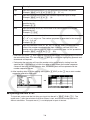
USB connector that comes with the fx-FD10 Pro
Power Graphic Unit to Windows® compatible PC
Declaration of Conformity
Model Number:
fx-FD10 Pro
Trade Name:
CASIO COMPUTER CO., LTD.
Responsible party: CASIO AMERICA, INC.
Address:
570 MT. PLEASANT AVENUE, DOVER, NEW JERSEY 07801
Telephone number:
973-361-5400
This device complies with Part 15 of the FCC Rules. Operation is subject to the
following two conditions: (1) This device may not cause harmful interference, and (2)
this device must accept any interference received, including interference that may
cause undesired operation.
i
Important!
The splash resistance and dust resistance performance of the calculator are based on CASIO
testing methods. Indicated performance is based on performance at the time of shipment from the
factory (at the time of delivery to you). CASIO makes no guarantee that such performance will be
provided in environments where you use the calculator. Also note that submersion in water during
use is not covered by the warranty, so be sure to take the same precautions that you take with
other electrical devices whenever using this calculator in the rain.
• The contents of this user’s guide are subject to change without notice.
• No part of this user’s guide may be reproduced in any form without the express written
consent of the manufacturer.
• Microsoft, Windows, and Windows Vista are registered trademarks or trademarks of Microsoft
Corporation in the United States and other countries.
• Mac OS is a trademark of Apple, Inc. in the United States and other countries.
• The SDHC Logo is a trademark of SD-3C, LLC.
• Company and product names used in this manual may be registered trademarks or
trademarks of their respective owners.
ii
Contents
Chapter 1 Getting Acquainted — Read This First!
1.
2.
3.
4.
5.
BEFORE USING THE CALCULATOR FOR THE FIRST TIME... ................................ 1-1
Handling Precautions .................................................................................................... 1-3
LCD and Key Back Lighting .......................................................................................... 1-6
Splash Resistance, Dust Resistance, and Shock Resistance ...................................... 1-7
About this User’s Guide ................................................................................................ 1-8
Chapter 2 Basic Operation
1.
2.
3.
4.
5.
6.
7.
8.
Keys .............................................................................................................................. 2-1
Display .......................................................................................................................... 2-3
Inputting and Editing Calculations ................................................................................. 2-6
Option (OPTN) Menu .................................................................................................. 2-11
Variable Data (VARS) Menu ....................................................................................... 2-12
Program (PRGM) Menu .............................................................................................. 2-13
Using the Setup Screen .............................................................................................. 2-14
When you keep having problems… ........................................................................... 2-16
Chapter 3 Manual Calculations
1.
2.
3.
4.
5.
6.
7.
8.
9.
Basic Calculations ......................................................................................................... 3-1
Special Functions .......................................................................................................... 3-4
Specifying the Angle Unit and Display Format .............................................................. 3-8
Function Calculations .................................................................................................. 3-10
Numerical Calculations ............................................................................................... 3-19
Complex Number Calculations.................................................................................... 3-28
Binary, Octal, Decimal, and Hexadecimal Calculations with Integers ......................... 3-31
Matrix Calculations ...................................................................................................... 3-34
Metric Conversion Calculations................................................................................... 3-48
Chapter 4 List Function
1.
2.
3.
4.
5.
Inputting and Editing a List ............................................................................................ 4-1
Manipulating List Data................................................................................................... 4-5
Arithmetic Calculations Using Lists ............................................................................. 4-10
Switching Between List Files....................................................................................... 4-12
Using CSV Files .......................................................................................................... 4-13
Chapter 5 Statistical Graphs and Calculations
1.
2.
3.
4.
5.
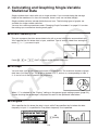
Before Performing Statistical Calculations .................................................................... 5-1
Calculating and Graphing Single-Variable Statistical Data ........................................... 5-4
Calculating and Graphing Paired-Variable Statistical Data ........................................... 5-9
Statistical Graph Display Operations .......................................................................... 5-14
Performing Statistical Calculations.............................................................................. 5-20
Chapter 6 Programming
1.
2.
3.
4.
5.
6.
7.
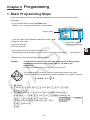
Basic Programming Steps............................................................................................. 6-1
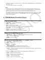
PRGM Mode Function Keys.......................................................................................... 6-3
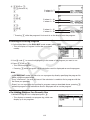
Editing Program Contents ............................................................................................. 6-4
File Management .......................................................................................................... 6-6
Command Reference .................................................................................................. 6-10
Using Calculator Functions in Programs ..................................................................... 6-26
PRGM Mode Command List ....................................................................................... 6-31
iii
8. CASIO Scientific Function Calculator Special Commands ⇔
Text Conversion Table ................................................................................................ 6-34
Chapter 7 Spreadsheet
1.
2.
3.
4.
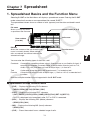
Spreadsheet Basics and the Function Menu ............................................................... 7-1
Basic Spreadsheet Operations ..................................................................................... 7-2
Using Special S • SHT Mode Commands .................................................................... 7-15
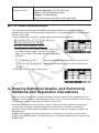
Drawing Statistical Graphs, and Performing Statistical and Regression
Calculations................................................................................................................. 7-16
5. S • SHT Mode Memory ................................................................................................ 7-21
Chapter 8 Memory Manager
1. Using the Memory Manager .......................................................................................... 8-1
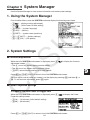
Chapter 9 System Manager
1. Using the System Manager ........................................................................................... 9-1
2. System Settings ............................................................................................................ 9-1
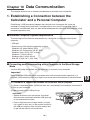
Chapter 10 Data Communication
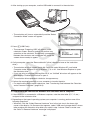
1. Establishing a Connection between the Calculator and a Personal Computer ........... 10-1
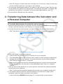
2. Transferring Data between the Calculator and a Personal Computer ........................ 10-3
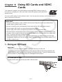
Chapter 11 Using SD Cards and SDHC Cards
1. Using an SD Card ....................................................................................................... 11-1
2. Formatting an SD Card ............................................................................................... 11-3
3. SD Card Precautions during Use ................................................................................ 11-3
Appendix
1.
2.
3.
4.
5.
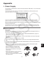
Power Supply ................................................................................................................α-1
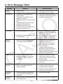
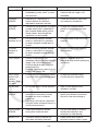
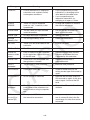
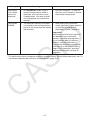
Error Message Table.....................................................................................................α-4
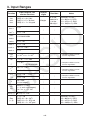
Input Ranges .................................................................................................................α-8
Specifications ..............................................................................................................α-10
Preset Programs .........................................................................................................α-12
iv
Chapter 1 Getting Acquainted
— Read This First!
1. BEFORE USING THE CALCULATOR FOR THE
FIRST TIME...
Batteries are not loaded in your calculator at the factory.
Be sure to follow the procedure below to load batteries and adjust the display contrast before
trying to use the calculator for the first time.
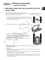
1. Turn over the calculator and rotate the center knob to the left.
• During the remainder of this procedure, take care that you do not
accidentally press the o key.
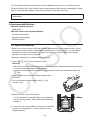
2. Lift up the battery compartment cover (1) and remove it (2).
2
1
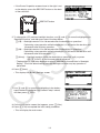
3. Load the four batteries that come with the calculator.
• When loading batteries other than those that come with the
calculator, be sure to load full set of four AAA-size alkaline or
rechargeable nickel-metal hydride batteries.
• Make sure that the positive (+) and negative (–) ends of the
batteries are facing correctly.
4. Replace the battery compartment cover. While pressing down on the cover, rotate the
center knob to the right.
Important!
• You may not be able to rotate the center knob if you do not press down on the battery
compartment cover as you do.
• Splash resistance, dust resistance, and shock resistance are maximized while the battery
compartment cover is fully and securely closed.
• Even a slight amount of foreign matter (a single hair, speck of dust, etc.) on the contact
surface of the battery compartment cover can allow moisture and/or dust to get into the
interior of the calculator.
1-1
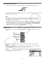
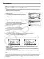
1
• If the Power Properties screen shown to the right is not
on the display, press the RESTART button on the back
of the calculator.
RESTART button
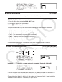
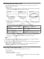
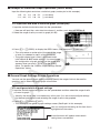
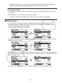
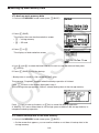
5. To change the LCD and key backlight duration, use c and f to move the highlighting to
“Backlight Duration” and then press one of the keys below.
1(10) ... Backlight remains lit for 10 seconds after the backlight on operation.*
Performing a key operation while the backlight is lit will restart the duration until
10 seconds after that key operation.
2(30) ... Backlight remains lit for 30 seconds after the backlight on operation.*
Performing a key operation while the backlight is lit will restart the duration until
30 seconds after that operation.
3(Alway) ... Backlight remains lit after the backlight on operation* until you press
!a(LIGHT) or until the calculator is turned off.
* The backlight on operation depends on what is selected for the calculator’s “Backlight
Setting”. The initial default setting turns the backlight on when any key operation is
performed.
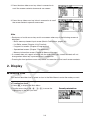
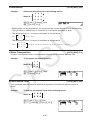
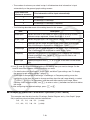
6. Press 6(Next).
• This displays the Battery Settings screen.
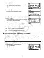
7. Use f and c to move the highlighting to the battery
type matches the batteries you loaded in step 2 above,
and then press 1(SEL).
8. On the confirmation screen that appears, press 1(Yes).
9. Press 6(FIN) to complete the initial setup procedure.
• This will display the main menu.
1-2
2. Handling Precautions
• Your calculator is made up of precision components. Never try to take it apart.
• Avoid dropping your calculator and subjecting it to strong impact.
• Do not store the calculator or leave it in areas exposed to high temperatures or humidity, or
large amounts of dust. When exposed to low temperatures, the calculator may require more
time to display results and may even fail to operate. Correct operation will resume once the
calculator is brought back to normal temperature.
• Your calculator supports use of both alkaline batteries and rechargeable nickel-metal hydride
batteries. Note that the amount of operation between charges provided by nickel-metal
hydride batteries is shorter than the life of alkaline batteries. Use only batteries that are
specifically recommended for this calculator.
• Replace the main batteries once every one year regardless of how much the calculator
is used during that period. Never leave dead batteries in the battery compartment. They
can leak and damage the unit. Immediately remove nickel-metal hydride batteries from the
calculator after their charge is used up. Leaving uncharged nickel-metal hydride batteries in
the calculator can cause them to deteriorate.
• Keep batteries out of the reach of small children. If swallowed, consult a physician
immediately.
• Avoid using volatile liquids such as thinner or benzine to clean the unit. Wipe it with a soft,
dry cloth, or with a cloth that has been moistened with a solution of water and a neutral
detergent and wrung out.
• Always be gentle when wiping dust off the display to avoid scratching it.
• In no event will the manufacturer and its suppliers be liable to you or any other person for
any damages, expenses, lost profits, lost savings or any other damages arising out of loss
of data and/or formulas arising out of malfunction, repairs, or battery replacement. It is up to
you to prepare physical records of data to protect against such data loss.
• Never dispose of batteries, the liquid crystal panel, or other components by burning them.
• Be sure that the power switch is set to OFF when replacing batteries.
• If the calculator is exposed to a strong electrostatic charge, its memory contents may be
damaged or the keys may stop working. In such a case, perform the Reset operation to clear
the memory and restore normal key operation.
• If the calculator stops operating correctly for some reason, use a thin, pointed object to press
the RESTART button on the back of the calculator. Note, however, that this clears all the
data in calculator memory.
• Note that strong vibration or impact during program execution can cause execution to stop or
can damage the calculator’s memory contents.
• Using the calculator near a television or radio can cause interference with TV or radio
reception.
• Before assuming malfunction of the unit, be sure to carefully reread this User’s Guide and
ensure that the problem is not due to insufficient battery power, programming or operational
errors.
• Avoid contact with water and other liquids.
Though your calculator is designed to be splash-resistant, note that splash-resistance is
reduced if it is exposed to moisture, dirt, or dust while the battery compartment cover, USB
port cap, SD card cap, or other opening is uncovered. Moisture getting into the calculator
creates the risk of malfunction, fire, and electric shock.
1-3
• Do not swing the calculator around by its strap. Doing so creates the risk of calculator
malfunction and personal injury.
• Avoid opening the battery compartment cover, USB port cap, and SD card cap in areas
where moisture or salt wind is present, when your hands are wet, when wearing wet gloves,
etc.
• Periodically check the battery compartment cover, USB port cap, SD card cap, and the areas
around them for dirt, sand, and other foreign matter. If any of these areas are dirty, use a
soft, clean, and dry cloth to wipe them. Note that even a minute particle of foreign matter (a
single strand of hair, a single grain of sand, etc.) on a cover or cap contact surface creates
the risk of moisture reaching the calculator interior.
• If the calculator is exposed to large amounts of rain or other water, wipe it dry. Make sure
that all moisture is removed before using the calculator again.
• Do not use the calculator for long periods in the rain.
• When closing the battery compartment cover, USB port cap, or SD card cap, inspect its
gasket for cracks, damage, looseness, or other irregularities, and make sure that the cover
or cap closes securely.
• Take care to avoid dropping the calculator and do not leave it in an area that is outside the
allowable operating temperature range. Such conditions can cause deterioration of splash
and/or dust resistance.
• Calculator accessories and options are not splash or dust resistant.
• Subjecting the calculator to extreme shock may cause loss of splash and/or dust resistance.
• CASIO COMPUTER CO., LTD. shall held in no way liable for any malfunction of or damage
to the calculator or SD card being used, or for any corruption or deletion of memory contents
due to problems related to invasion of moisture that may occur due to misuse by you.
• CASIO COMPUTER CO., LTD. shall not be held responsible for any problems caused by
exposure of this calculator to moisture.
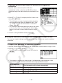
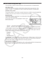
• A progress bar and/or a busy indicator appear on the display whenever the calculator is
performing a calculation, writing to memory, or reading from memory.
Busy indicator
Progress bar
Never press the RESTART button or remove the batteries from the calculator when the
progress bar or busy indicator is on the display. Doing so can cause memory contents to be
lost and can cause malfunction of the calculator.
1-4
Be sure to keep physical records of all important data!
The large memory capacity of the unit makes it possible to store large amounts of data.
You should note, however, that low battery power or incorrect replacement of the batteries
that power the unit can cause the data stored in memory to be corrupted or even lost entirely.
Stored data can also be affected by strong electrostatic charge or strong impact. It is up to you
to keep back up copies of data to protect against its loss.
Since this calculator employs unused memory as a work area when performing its internal
calculations, an error may occur when there is not enough memory available to perform
calculations. To avoid such problems, it is a good idea to leave 1 or 2 kbytes of memory free
(unused) at all times.
In no event shall CASIO Computer Co., Ltd. be liable to anyone for special, collateral,
incidental, or consequential damages in connection with or arising out of the purchase or use
of these materials. Moreover, CASIO Computer Co., Ltd. shall not be liable for any claim of
any kind whatsoever against the use of these materials by any other party.
1-5
3. LCD and Key Back Lighting
This calculator is equipped with LCD and key back lighting to make the keys and display easy
to read, even in the dark. You can conserve battery power by limiting backlight operation to
only when you need it.
u To turn the backlight on or off
Press !a(LIGHT) to toggle the backlight on and off.
• Changing the Backlight On/Off Key
You can configure the calculator so the backlight turns on when any key is pressed, instead of
requiring the !a(LIGHT) to toggle the backlight on and off. For details, see “To specify
the backlight key” (page 9-2).
• Backlight duration
You can configure backlight settings so it remains on or turns off after a specific period (30
seconds or 10 seconds) of calculator non-use. See “To specify the backlight duration” for
details about the applicable operation procedure.
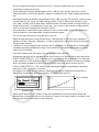
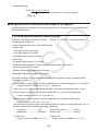
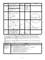
• Backlight and Battery Life
• Long-term backlight illumination can shorten battery life.
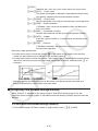
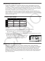
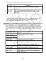
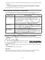
• The table below shows approximate battery life values for a new set of alkaline batteries or
a new set of nickel-metal hydride batteries when operations (1) through (3) are performed
repeatedly at one-hour intervals, under a temperature of 25°C.
(1) Five minutes of main menu display
(2) PRGM mode calculation for 5 minutes
(3) 50 minutes of PRGM mode display
Batteries
Alkaline
Nickel-metal
hydride batteries
(Recommended
batteries only)
Backlight Use
Approximate Battery Life
Lit for the first 30 seconds of the
three-step operation, then turned off
after that.
200 hours
Continuously lit.
25 hours
Lit for the first 30 seconds of the
three-step operation, then turned off
after that.
120 hours
(Reference value)
Continuously lit.
15 hours
(Reference value)
1-6
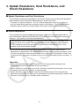
4. Splash Resistance, Dust Resistance, and
Shock Resistance
k Splash Resistance and Dust Resistance
This calculator satisfies the requirements of the IP54* splash proof and dust proof protection
levels defined by the International Electrotechnical Commission (IEC).
* IP stands for “ingress protection”. The “5” of the left digit means Class 5 (no ingress of
dust that affect device operation) protection against solid objects. The “4” means Class 4
protection against liquids (no harmful effects from water sprayed from all directions).
k Shock Resistance
This calculator has cleared independent testing by CASIO that was conducted based on
the United States Defense Department MIL-STD-810G shock resistance performance test
methods*. Test methods are those described below.
Local testing by natural dropping of the calculator to the floor (P tile on concrete) from a
height of 122 cm on six faces. Test data represents actual cumulative values based on
CASIO standards, and do not constitute any guarantee of non-destruction of or nondamage to the actual product exterior.
* Environmental laboratory test method (Method 516.6-Shock) of the United States
Department of Defense MIL-STD-810G military standard, which requires passage by a total
of at least five devices, which are drop tested from a height of 122 centimeters (4 feet) onto
a plywood (lauan) drop zone, in groups of five, for a total of 26 drops (6 faces, 8 corners, 12
edges)
Important!
• Shock resistance testing assumes exposure to shock during normal everyday use.
Subjecting the calculator to extreme shock may destroy it.
• Even if exposure to shock does not result in calculator operational performance, it can cause
scratching of the calculator’s display or other damage.
• Splash resistance, dust resistance, and shock resistance testing of this calculator was
performed using CASIO test methods. No guarantees are made concerning the ability of the
calculator to be impervious to damage and/or malfunction.
1-7
5. About this User’s Guide
u !x(')
The above indicates you should press ! and then x, which will input a ' symbol. All
multiple-key input operations are indicated like this. Key cap markings are shown, followed by
the input character or command in parentheses.
u m STAT
This indicates you should first press m, use the cursor keys (f, c, d, e) to select the
STAT mode, and then press w. Operations you need to perform to enter a mode from the
Main Menu are indicated like this.
u Function Keys and Menus
• Many of the operations performed by this calculator can be executed by pressing function
keys 1 through 6. The operation assigned to each function key changes according to
the mode the calculator is in, and current operation assignments are indicated by function
menus that appear at the bottom of the display.
• This User’s Guide shows the current operation assigned to a function key in parentheses
following the key cap for that key. 1(Comp), for example, indicates that pressing 1
selects {Comp}, which is also indicated in the function menu.
• When (g) is indicated in the function menu for key 6, it means that pressing 6 displays
the next page or previous page of menu options.
u Menu Titles
• Menu titles in this User’s Guide include the key operation required to display the menu
being explained. The key operation for a menu that is displayed by pressing K and then
{LIST} would be shown as: [OPTN]-[LIST].
• 6(g) key operations to change to another menu page are not shown in menu title key
operations.
u Command List
The PRGM Mode Command List (page 6-31) provides a graphic flowchart of the various
function key menus and shows how to maneuver to the menu of commands you need.
Example: The following operation displays Xfct: [VARS]-[FACT]-[Xfct]
u E-CON2
This manual does not cover the E-CON2 mode. For more information about the E-CON2
mode, download the E-CON2 manual (English version only) from: http://edu.casio.com.
1-8
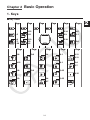
Chapter 2 Basic Operation
1. Keys
k Key Table
Page
Page
Page
2-12
2-14
α-2
2-2
2-11
2-3
1-1
1-6
2-7,
2-10
2-13
2-2,
6-2
2-10
Page
2-6
Page
Page
Page
2-6
Page
Page
2-6
3-4
Page
3-1
Page
3-11
3-11
3-12
3-1
3-4
2-7
2-8
2-9
3-15
3-12
2-9
3-4
3-7
2-1
3-15
2
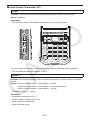
k Calculator Front Keys
Almost all of the keys on the front of the calculator have two functions assigned to them.
2
1
For example, pressing the x key directly inputs ^2 (1: square), while pressing ! and then
x inputs '(2: square root).
Note
• For information about keys 1 through 6, see “About the Function Menu” (page 2-5).
• The a key is used when inputting alphabetic characters. See “Inputting Alphabetic
Characters” for more information.
• Pressing the a key twice in succession displays a function menu of up to six functions
or commands registered by you to the Favorites category. You can use the function menu
to input Favorites functions and commands. For more information, see “To input Favorites
category commands using the function keys” (page 2-11).
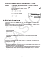
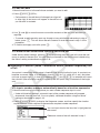
k Side Keys
There are three keys on the right side of the calculator: up cursor key, down cursor key, and
w key.
Up cursor key
Down cursor key
w key
These keys perform the same operations as the corresponding keys on the front of the
calculator.
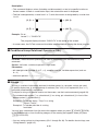
As shown in the example below, the up and down cursor keys can be used to scroll certain
screens one screen by pressing one of the keys twice in succession.
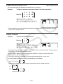
Example
To use the up and down cursor keys to scroll a program list one screen
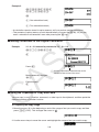
1. Press 0 to display the program list.
2-2
2. Press the down side cursor key twice in succession to
scroll the screen contents downwards one screen.
3. Press the up side cursor key twice in succession to scroll
the screen contents upwards one screen.
Note
• Each press of a side cursor key scrolls one screen when any of the following screens is
displayed.
- Matrix memory element input screen (Matrix Calculations, page 3-34)
- List Editor screen (Chapter 4 List Function)
- Program List screen (Chapter 6 Programming)
- Spreadsheet screen (Chapter 7 Spreadsheet)
- Memory information screen (Chapter 8 Memory Manager)
• If a screen does not support scrolling with the side cursor keys, screen contents will not
change when either key is pressed twice in succession.
• Pressing the front up/down cursor keys twice in succession will not scroll screen contents.
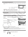
2. Display
k Selecting Icons
This section describes how to select an icon in the Main Menu to enter the mode you want.
u To select an icon
1. Press m to display the Main Menu.
2. Use the cursor keys (d, e, f, c) to move the
highlighting to the icon you want.
2-3
Currently selected icon
3. Press w to display the initial screen of the mode
whose icon you selected. Here we will enter the
STAT mode.
• You can also enter a mode without highlighting an icon in the Main Menu by inputting the
number marked in the lower right corner of the icon.
• Use only the procedures described above to enter a mode. If you use any other procedure,
you may end up in a mode that is different than the one you thought you selected.
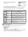
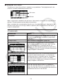
The following explains the meaning of each icon.
Icon
Mode Name
RUN • MAT
(Run • Matrix)
PRGM
(Program)
STAT
(Statistics)
S • SHT
(Spreadsheet)
Description
Use this mode for arithmetic calculations and function
calculations, and for calculations involving binary, octal,
decimal, and hexadecimal values and matrices.
Use this mode to write, store and recall programs that be
reused for calculation as required. A variety of different useful
preset programs are provided.
Use this mode to perform single-variable (standard deviation)
and paired-variable (regression) statistical calculations, to
perform tests, to analyze data and to draw statistical graphs.
Use this mode to perform spreadsheet calculations. You can
also perform the same statistical calculations and statistical
graphing operations you perform in the STAT mode.
MEMORY
Use this mode to manage data in the calculator’s main
memory and storage memory, and on an SD card loaded in
the calculator.
SYSTEM
Use this mode to adjust display contrast, and to configure
power supply, display language, memory reset, and other
general operational settings.
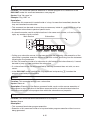
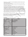
k Battery Level Indicator
An icon in the upper right corner of the Main Menu (m) shows approximately how much
battery power is remaining.
... From left to right: Level 3, Level 2, Level 1, Dead.
Important!
• Replace batteries as soon as possible whenever
(Level 1) is indicated. For information
about battery replacement, see “Replacing Batteries” (page Ơ-1).
• The calculator will display a message prompting you to replace batteries when battery power
goes very low. For more information, see “Low Battery Message” (page 2-17).
2-4
k About the Function Menu
Use the function keys (1 to 6) to access the menus and commands in the menu bar
along the bottom of the display screen. You can tell whether a menu bar item is a menu or a
command by its appearance.
k Normal Display
The calculator normally displays values up to 10 digits long. Values that exceed this limit are
automatically converted to and displayed in exponential format.
u How to interpret exponential format
1.2E+12 indicates that the result is equivalent to 1.2 × 1012. This means that you should move
the decimal point in 1.2 twelve places to the right, because the exponent is positive. This
results in the value 1,200,000,000,000.
1.2E–03 indicates that the result is equivalent to 1.2 × 10–3. This means that you should move
the decimal point in 1.2 three places to the left, because the exponent is negative. This results
in the value 0.0012.
You can specify one of two different ranges for automatic changeover to normal display.
Norm 1 ................... 10–2 (0.01) > |x|, |x| > 1010
Norm 2 ................... 10–9 (0.000000001) > |x|, |x| > 1010
All of the examples in this manual show calculation results using Norm 1.
See page 3-9 for details on switching between Norm 1 and Norm 2.
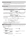
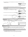
k Special Display Formats
This calculator uses special display formats to indicate fractions, hexadecimal values, and
degrees/minutes/seconds values.
u Fractions
.................... Indicates: 456
12
23
u Hexadecimal Values
................... Indicates: 0ABCDEF1(16), which equals
180150001(10)
u Degrees/Minutes/Seconds
.................... Indicates: 12° 34’ 56.78”
2-5
• In addition to the above, this calculator also uses other indicators or symbols, which are
described in each applicable section of this manual as they come up.
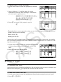
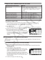
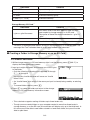
3. Inputting and Editing Calculations
k Inputting Calculations
When you are ready to input a calculation, first press A to clear the display. Next, input your
calculation formulas exactly as they are written, from left to right, and press w to obtain the
result.
Example
2 + 3 – 4 + 10 =
Ac+d-e+baw
k Editing Calculations
Use the d and e keys to move the cursor to the position you want to change, and then
perform one of the operations described below. After you edit the calculation, you can execute
it by pressing w. Or you can use e to move to the end of the calculation and input more.
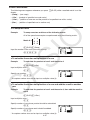
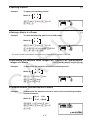
u To change a step
Example
To change cos60 to sin60
A!i(cos)ga
ddd
D
!h(sin)
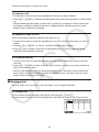
u To delete a step
Example
To change 369 × × 2 to 369 × 2
Adgj**c
dD
In the insert mode, the D key operates as a backspace key.
2-6
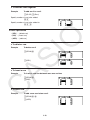
u To insert a step
Example
To change 2.362 to sin2.362
Ac.dgx
ddddd
!h(sin)
k Alphabetic Character Input
Use the function menu that appears when you press a to input alphabetic characters for
variable memory names (A through Z), program names, etc.
Example
To input A + B + C
a1(A-E)1(A)+2(B)+3(C)
Note
To input symbols (', ", ~, =) and spaces, use the function menu that appears after you press
a6(SYBL).
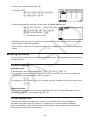
k Using Replay Memory
The last calculation performed is always stored into replay memory. You can recall the
contents of the replay memory by pressing d or e.
If you press e, the calculation appears with the cursor at the beginning. Pressing d causes
the calculation to appear with the cursor at the end. You can make changes in the calculation
as you wish and then execute it again.
Example 1
To perform the following two calculations
4.12 × 6.4 = 26.368
4.12 × 7.1 = 29.252
Ae.bc*g.ew
dDDD
h.b
w
After you press A, you can press f or c to recall previous calculations, in sequence from
the newest to the oldest (Multi-Replay Function). Once you recall a calculation, you can use
e and d to move the cursor around the calculation and make changes in it to create a new
calculation.
2-7
Example 2
Abcd+efgw
cde-fghw
A
f (One calculation back)
f (Two calculations back)
• A calculation remains stored in replay memory until you perform another calculation.
• The contents of replay memory are not cleared when you press the A key, so you can
recall a calculation and execute it even after pressing the A key.
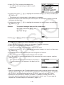
k Making Corrections in the Original Calculation
Example
14 ÷ 0 × 2.3 entered by mistake for 14 ÷ 10 × 2.3
Abe/a*c.d
w
Press J.
Cursor is positioned automatically at the
location of the cause of the error.
Make necessary changes.
db
Execute again.
w
k Using the Clipboard for Copy and Paste
You can copy (or cut) a function, command, or other input to the clipboard, and then paste the
clipboard contents at another location.
u To specify the copy range
1. Move the cursor (I) to the beginning or end of the range of text you want to copy and then
press !b(CLIP). This changes the cursor to “ ”.
2. Use the cursor keys to move the cursor and highlight the range of text you want to copy.
2-8
3. Press 1(COPY) to copy the highlighted text to the clipboard, and exit the copy range
specification mode.
The selected characters are not
changed when you copy them.
To cancel text highlighting without performing a copy operation, press J.
u To cut the text
1. Move the cursor (I) to the beginning or end of the range of text you want to cut and then
press !b(CLIP). This changes the cursor to “ ”.
2. Use the cursor keys to move the cursor and highlight the range of text you want to cut.
3. Press 2(CUT) to cut the highlighted text to the clipboard.
Cutting causes the original
characters to be deleted.
u Pasting Text
Move the cursor to the location where you want to paste the text, and then press
!c(PASTE). The contents of the clipboard are pasted at the cursor position.
A
!c(PASTE)
k Catalog Function
The Catalog is an alphabetic list of all the commands available on this calculator. You can
input a command by calling up the Catalog and then selecting the command you want.
Registering often-used commands to Favorites makes them more easily accessible for input.
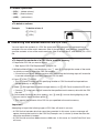
u To use the Catalog to input a command
1. Press !a(CATALOG) to display an alphabetic Catalog of commands.
• The screen that appears first is the last one you used for command input.
2-9
2. Press 6(CTGY) to display the category list.
• You can skip this step and go straight to step 5,
if you want.
3. Use the cursor keys (f, c) to highlight the command category you want, and then press
1(EXE) or w.
• This displays a list of commands in the category you selected.
4. Input the first letter of the command you want to input. This will display the first command
that starts with that letter.
5. Use the cursor keys (f, c) to highlight the command you want to input, and then press
1(INPUT) or w.
Example
To use the Catalog to input the ClrList command
A!a(CATALOG)a1(A-E)
3(C)c~cw
Pressing J or !J(QUIT) closes the Catalog.
u To register a frequently used commend to Favorites
1. Press !a(CATALOG) to display an alphabetic Catalog of commands.
2. Press 6(CTGY) to display the category list.
• You can skip this step and go straight to step 5, if you want.
3. Use the cursor keys (f, c) to highlight the command category you want, and then press
1(EXE) or w.
4. Input the first letter of the command you want to register to Favorites.
• This will display the first command that begins with that letter.
5. Use f and c to move the highlighting to the command you want to register, and then
press 2(FAV).
• This registers the highlighted command to Favorites. A
Favorites category list will appear on the display at this
time.
Note
• The first six commands in the Favorites category can be input using the function menu that
appears when the a key is pressed twice in succession. The top command is assigned to
key 1(FAV1), the second command to key 2(FAV2), and so on up to 6(FAV6).
• Each time a new command is added to Favorites, it is added to the end of the list. For
information about changing the order of the commands in the list, see “To re-arrange the
sequence of Favorites category list commands” (page 2-11).
2-10
u To input Favorites category commands using the function keys
1. Press the a key twice.
• This displays a function menu for inputting Favorites
category commands.
2. Press the function key (1(FAV1) to 6(FAV6)) that corresponds to the command you
want to input.
u To re-arrange the sequence of Favorites category list commands
1. Press !a(CATALOG) to display the catalog screen, and then press 6(CTGY)c to
display the Favorites category list.
2. Use f and c to move the highlighting to one of
the commands you want to move, and then press
2(SWAP).
3. Use f and c to move the highlighting to the
command you want to swap with the command you
selected above, and then press 2(SWAP).
u To delete a command from the Favorites category
While the Favorites category list is displayed, use f and c to move the highlighting to the
command you want to delete, and then press 5(DEL).
4. Option (OPTN) Menu
The option menu gives you access to scientific functions and features that are not marked on
the calculator’s keyboard. The contents of the option menu differ according to the mode you
are in when you press the K key.
• The option menu does not appear if you press K while binary, octal, decimal, or
hexadecimal is set as the default number system.
• For details about the commands included on the option (OPTN) menu, see the “K key”
item in the “PRGM Mode Command List” (page 6-31).
• The meanings of the option menu items are described in the sections that cover each mode.
The following list shows the option menu that is displayed when the RUN • MAT or PRGM
mode is selected.
• {LIST} ... {list function menu}
• {MAT} ... {matrix operation menu}
• {CPLX} ... {complex number calculation menu}
• {CALC} ... {functional analysis menu}
2-11
• {STAT} ... {menu for paired-variable statistical estimated value}
• {CONV} ... {metric conversion menu}
• {HYP} ... {hyperbolic calculation menu}
• {PROB} ... {probability/distribution calculation menu}
• {NUM} ... {numeric calculation menu}
• {ANGL} ... {menu for angle/coordinate conversion, sexagesimal input/conversion}
• {ESYM} ... {engineering symbol menu}
• {PICT} ... {graph save/recall menu}
• {FMEM} ... {function memory menu}
• {LOGIC} ... {logic operator menu}
5. Variable Data (VARS) Menu
To recall variable data, press !K(VARS) to display the variable data menu.
{V-WIN}/{FACT}/{STAT}/{Str}
• Note that the Str item appears for function key 6 only when you access the variable data
menu from the RUN • MAT or PRGM mode.
• The variable data menu does not appear if you press !K(VARS) while binary, octal,
decimal, or hexadecimal is set as the default number system.
• For details about the commands included on the variable data (VARS) menu, see the
“!K(VARS) key” item in the “PRGM Mode Command List” (page 6-31).
u V-WIN — Recalling V-Window values
• {X}/{Y} ... {x-axis menu}/{y-axis menu}
• {min}/{max}/{scal}/{dot} ... {minimum value}/{maximum value}/{scale}/{dot value*1}
*1 The dot value indicates the display range (Xmax value – Xmin value) divided by the
screen dot pitch (126). The dot value is normally calculated automatically from the
minimum and maximum values. Changing the dot value causes the maximum to be
calculated automatically.
u FACT — Recalling zoom factors
• {Xfct}/{Yfct} ... {x-axis factor}/{y-axis factor}
u STAT — Recalling statistical data
• {X} … {single-variable, paired-variable x-data}
• {n}/{x
¯ }/{Σx}/{Σx2}/{Ʊx}/{sx}/{minX}/{maxX} ... {number of data}/{mean}/{sum}/{sum
of squares}/{population standard deviation}/{sample standard deviation}/{minimum
value}/{maximum value}
• {Y} ... {paired-variable y-data}
• {Κ}/{Σy}/{Σy2}/{Σxy}/{Ʊx}/{sy}/{minY}/{maxY} ... {mean}/{sum}/{sum of squares}/{sum
of products of x-data and y-data}/{population standard deviation}/{sample standard
deviation}/{minimum value}/{maximum value}
2-12
• {GRPH} ... {graph data menu}
• {a}/{b}/{c}/{d}/{e} ... {regression coefficient and polynomial coefficients}
• {r}/{r2} ... {correlation coefficient}/{coefficient of determination}
• {MSe} ... {mean square error}
• {Q1}/{Q3} ... {first quartile}/{third quartile}
• {Med}/{Mod} ... {median}/{mode} of input data
• {Strt}/{Pitch} ... histogram {start division}/{pitch}
• {PTS} ... {summary point data menu}
• {x1}/{y1}/{x2}/{y2}/{x3}/{y3} ... {coordinates of summary points}
u Str — Str command
• {Str} ... {string memory}
6. Program (PRGM) Menu
To display the program (PRGM) menu, first enter the RUN • MAT or PRGM mode from the
Main Menu and then press !0(PRGM). The following are the selections available in
the program (PRGM) menu.
• {COM} ...... {program command menu}
• {CTL} ....... {program control command menu}
• {JUMP} ..... {jump command menu}
• {?} ............ {input command}
• {^} .......... {output command}
• {CLR} ....... {clear command menu}
• {DISP} ...... {display command menu}
• {REL} ....... {conditional jump relational operator menu}
• {I/O} ......... {I/O control/transfer command menu}
• {:} ............. {multi-statement command}
• {STR} ....... {string command}
The following function key menu appears if you press !0(PRGM) in the RUN • MAT
mode or the PRGM mode while binary, octal, decimal, or hexadecimal is set as the default
number system.
• {Prog} ....... {program recall}
• {JUMP}/{?}/{^}/{REL}/{:}
The functions assigned to the function keys are the same as those in the Comp mode.
For details on the commands that are available in the various menus you can access from the
program menu, see “Chapter 6 Programming”.
2-13
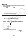
7. Using the Setup Screen
The mode’s Setup screen shows the current status of mode settings and lets you make any
changes you want. The following procedure shows how to change a setup.
u To change a mode setup
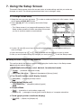
1. Select the icon you want and press w to enter a mode and display its initial screen. Here
we will enter the RUN • MAT mode.
2. Press !m(SET UP) to display the mode’s Setup
screen.
• This Setup screen is just one possible example. Actual
Setup screen contents will differ according to the mode
you are in and that mode’s current settings.
3. Use the f and c cursor keys to move the highlighting to the item whose setting you
want to change.
4. Press the function key (1 to 6) that is marked with the setting you want to make.
5. After you are finished making any changes you want, press J to exit the Setup screen.
k Setup Screen Function Key Menus
This section details the settings you can make using the function keys in the Setup screen.
indicates default setting.
u Mode (calculation/binary, octal, decimal, hexadecimal mode)
• {Comp} ... {arithmetic calculation mode}
• {Dec}/{Hex}/{Bin}/{Oct} ... {decimal}/{hexadecimal}/{binary}/{octal}
u Frac Result (fraction result display format)
• {d/c}/{ab/c} ... {improper}/{mixed} fraction
u Angle (default angle unit)
• {Deg}/{Rad}/{Gra} ... {degrees}/{radians}/{grads}
u Complex Mode
• {Real} ... {calculation in real number range only}
• {a+bi}/{r∠Ƨ} ... {rectangular format}/{polar format} display of a complex calculation
u Coord (graph pointer coordinate display)
• {On}/{Off} ... {display on}/{display off}
2-14
u Grid (graph gridline display)
• {On}/{Off} ... {display on}/{display off}
u Axes (graph axis display)
• {On}/{Off} ... {display on}/{display off}
u Label (graph axis label display)
• {On}/{Off} ... {display on}/{display off}
u Display (display format)
• {Fix}/{Sci}/{Norm}/{Eng} ... {fixed number of decimal places specification}/{number of
significant digits specification}/{normal display setting}/{engineering mode}
u Simplify (calculation result auto/manual reduction specification)
• {Auto}/{Man} ... {auto reduce and display}/{display without reduction}
u Stat Wind (statistical graph V-Window setting method)
• {Auto}/{Man} ... {automatic}/{manual}
u Resid List (residual calculation)
• {None}/{LIST} ... {no calculation}/{list specification for the calculated residual data}
u List File (list file display settings)
• {FILE} ... {settings of list file on the display}
u Sub Name (list naming)
• {On}/{Off} ... {display on}/{display off}
u Graph Func (graph name display during graph drawing and trace)
• {On}/{Off} ... {display on}/{display off}
u Background (graph display background)
• {None}/{PICT} ... {no background}/{graph background picture specification}
u Sketch Line (overlaid line type)
•{
}/{
}/{
}/{
} ... {normal}/{thick}/{broken}/{dotted}
u Q1Q3 Type (Q1/Q3 calculation formulas)
• {Std}/{OnD} ... {Divide total population on its center point between upper and lower
groups, with the median of the lower group Q1 and the median of the upper group Q3}/
{Make the value of element whose cumulative frequency ratio is greater than 1/4 and
nearest to 1/4 Q1 and the value of element whose cumulative frequency ratio is greater
than 3/4 and nearest to 3/4 Q3}
u Auto Calc (spreadsheet auto calc)
• {On}/{Off} ... {execute}/{not execute} the formulas automatically
u Show Cell (spreadsheet cell display mode)
• {Form}/{Val} ... {formula}*1/{value}
2-15
u Move (spreadsheet cell cursor direction)*2
• {Low}/{Right} ... {move down}/{move right}
*1 Selecting “Form” (formula) causes a formula in the cell to be displayed as a formula. The
“Form” does not affect any non-formula data in the cell.
*2 Specifies the direction the cell cursor moves when you press the w key to register cell
input, when the Sequence command generates a number table, and when you recall data
from List memory.
8. When you keep having problems…
If you keep having problems when you are trying to perform operations, try the following
before assuming that there is something wrong with the calculator.
k Getting the Calculator Back to its Original Mode Settings
1. From the Main Menu, enter the SYSTEM mode.
2. Press 5(RSET).
3. Press 1(STUP), and then press 1(Yes).
4. Press Jm to return to the Main Menu.
Now enter the correct mode and perform your calculation again, monitoring the results on the
display.
k Restart and Reset
u Restart
Should the calculator start to act abnormally, you can restart it by pressing the RESTART
button. Note, however, that you should only use the RESTART button only as a last resort.
Normally, pressing the RESTART button reboots the calculator’s operating system, so
programs and other data in calculator memory is retained.
RESTART button
2-16
Important!
The calculator backs up user data (main memory) when you turn power off and loads the
backed up data when you turn power back on.
When you press the RESTART button, the calculator restarts and loads backed up data.
This means that if you press the RESTART button after you edit a program or other data, any
data that has not been backed up will be lost.
u Reset
Use reset when you want to delete all data currently in calculator memory and return all mode
settings to their initial defaults.
Before performing the reset operation, first make a written copy of all important data.
For details, see “Reset” (page 9-3).
k Low Battery Message
If the following message appears on the display, immediately turn off the calculator and
replace batteries as instructed.
If you continue using the calculator without replacing batteries, power will automatically turn
off to protect memory contents. Once this happens, you will not be able to turn power back on,
and there is the danger that memory contents will be corrupted or lost entirely.
• You will not be able to perform data communications operations after the low battery
message appears.
2-17
Chapter 3 Manual Calculations
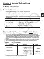
1. Basic Calculations
k Arithmetic Calculations
• Enter arithmetic calculations as they are written, from left to right.
• Use the - key to input the minus sign before a negative value.
• Calculations are performed internally with a 15-digit mantissa. The result is rounded to a 10digit mantissa before it is displayed.
• For mixed arithmetic calculations, multiplication and division are given priority over addition
and subtraction.
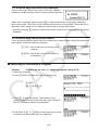
Example
Operation
56 × (–12) ÷ (–2.5) = 268.8
56*-12/-2.5w
(2 + 3) × 102 = 500
!*( ( ) 2+3!/( ) )*10xw
2 + 3 × (4 + 5) = 29
2+3*!*( ( ) 4+5w*1
6
= 0.3
4×5
6/!*( ( ) 4*5!/( ) )w
*1 Final closed parentheses (immediately before operation of the w key) may be omitted, no
matter how many are required.
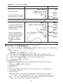
k Number of Decimal Places, Number of Significant Digits, Normal
Display Range
[SET UP]- [Display] -[Fix] / [Sci] / [Norm]
• Even after you specify the number of decimal places or the number of significant digits,
internal calculations are still performed using a 15-digit mantissa, and displayed values are
stored with a 10-digit mantissa. Use Rnd of the Numeric Calculation Menu (NUM) (page
3-10) to round the displayed value off to the number of decimal place and significant digit
settings.
• Number of decimal place (Fix) and significant digit (Sci) settings normally remain in effect
until you change them or until you change the normal display range (Norm) setting.
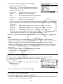
Example 1
100 ÷ 6 = 16.66666666...
Condition
Operation
Display
100/6w
16.66666667
4 decimal places
!m(SET UP) ff
1(Fix)ewJw
*1
16.6667
5 significant digits
!m(SET UP) ff
2(Sci)fwJw
*1E+01
1.6667
Cancels specification
!m(SET UP) ff
3(Norm)Jw
16.66666667
*1 Displayed values are rounded off to the place you specify.
3-1
3
Example 2
200 ÷ 7 × 14 = 400
Condition
Operation
3 decimal places
Calculation continues using
display capacity of 10 digits
Display
200/7*14w
400
!m(SET UP) ff
1(Fix)dwJw
400.000
200/7w
*
14w
28.571
Ans × I
400.000
• If the same calculation is performed using the specified number of digits:
200/7w
28.571
The value stored internally is
rounded off to the number of
decimal places specified on
the Setup screen.
K6(g)4(NUM)4(Rnd)w
*
14w
28.571
Ans × I
399.994
200/7w
28.571
You can also specify the
number of decimal places for
rounding of internal values
for a specific calculation.
(Example: To specify
rounding to two decimal
places)
6(g)1(RndFi)K,2!/( ) )
w
*
14w
RndFix(Ans,2)
28.570
Ans × I
399.980
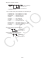
k Calculation Priority Sequence
This calculator employs true algebraic logic to calculate the parts of a formula in the following
order:
1 Type A functions
• Coordinate transformation Pol (x, y), Rec (r, θ)
• Functions that include parentheses (such as derivatives, integrations, Σ, etc.)
d/dx, d2/dx2, ∫dx, Σ, Solve, FMin, FMax, List→Mat, Fill, Seq, SortA, SortD, Min, Max,
Median, Mean, Augment, Mat→List, P(, Q(, R(, t(, RndFix, logab
• Composite functions*1, List, Mat, fn
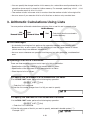
2 Type B functions
With these functions, the value is entered and then the function key is pressed.
x2, x–1, x!, ° ’ ”, ENG symbols, angle unit °, r, g
3 Power/root ^(xy), x'
4 Fractions a b/c
5 Abbreviated multiplication format in front of π, memory name, or variable name.
2π, 5A, Xmin, H Start, etc.
6 Type C functions
With these functions, the function key is pressed and then the value is entered.
', 3', log, In, ex, 10x, sin, cos, tan, sin–1, cos–1, tan–1, sinh, cosh, tanh, sinh–1, cosh–1,
tanh–1, (–), d, h, b, o, Neg, Not, Det, Trn, Dim, Identity, Ref, Rref, Sum, Prod, Cuml,
Percent, AList, Abs, Int, Frac, Intg, Arg, Conjg, ReP, ImP
3-2
7 Abbreviated multiplication format in front of Type A functions, Type C functions, and
parenthesis.
2'
3, A log2, etc.
8 Permutation, combination nPr, nCr
9 Metric conversion commands
0 ×, ÷, Int÷, Rnd
! +, –
@ Relational operators =, ≠, >, <, ≥, ≤
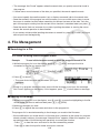
# And (logical operator), and (bitwise operator)
$ Or, Xor (logical operator), or, xor, xnor (bitwise operator)
*1 You can combine the contents of multiple function memory (fn) locations into composite
functions. Specifying fn1(fn2), for example, results in the composite function fn1°fn2. A
composite function can consist of up to five functions.
Example
2 + 3 × (log sin2π2 + 6.8) = 22.07101691 (angle unit = Rad)
1
2
3
4
5
6
• You cannot use a differential, quadratic differential, integration, Σ, maximum/minimum value,
Solve, RndFix or logab calculation expression inside of a RndFix calculation term.
• When functions with the same priority are used in series, execution is performed from right to
left.
exIn 120 → ex{In( 120)}
Otherwise, execution is from left to right.
• Compound functions are executed from right to left.
• Anything contained within parentheses receives highest priority.
k Multiplication Operations without a Multiplication Sign
You can omit the multiplication sign (×) in any of the following operations.
• Before Type A functions (1 on page 3-2) and Type C functions (6 on page 3-2), except for
negative signs
Example 1
3, 2Pol(5, 12), etc.
2sin30, 10log1.2, 2'
• Before constants, variable names, memory names
Example 2
2π, 2AB, 3Ans, etc.
• Before an open parenthesis
Example 3
3(5 + 6), (A + 1)(B – 1), etc.
Note
If you execute a calculation that includes both division and multiplication operations in which
a multiplication sign has been omitted, parentheses will be inserted automatically as shown in
the examples below.
3-3
• When a multiplication sign is omitted immediately before an open parenthesis or after a
closed parenthesis.
Example 1
6 ÷ 2(1 + 2) → 6 ÷ (2(1 + 2))
6 ÷ A(1 + 2) → 6 ÷ (A(1 + 2))
1 ÷ (2 + 3)sin30 → 1 ÷ ((2 + 3)sin30)
• When a multiplication sign is omitted immediately before a variable, a constant, etc.
Example 2
6 ÷ 2π
→
6 ÷ (2π)
2 ÷ 2'
2 → 2 ÷ (2'
2)
4π ÷ 2π
→
4π ÷ (2π)
k Overflow and Errors
Exceeding a specified input or calculation range, or attempting an illegal input causes an error
message to appear on the display. Further operation of the calculator is impossible while an
error message is displayed. For details, see the “Error Message Table” on page α-4.
• Most of the calculator’s keys are inoperative while an error message is displayed. Press J
to clear the error and return to normal operation.
k Memory Capacity
Each time you press a key, either one byte or two bytes is used. Some of the functions that
require one byte are: b, c, d, !h(sin), !i(cos), !j(tan), and !x(').
Some of the functions that take up two bytes are d/dx(, Mat, Xmin, If, For, Return, and SortA.
2. Special Functions
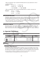
k Calculations Using Variables
Example
Operation
Display
193.2!K(→)a1(A-E)1(A)w
193.2
193.2 ÷ 23 = 8.4
1(A)/23w
8.4
193.2 ÷ 28 = 6.9
1(A)/28w
6.9
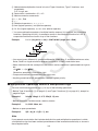
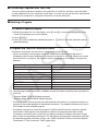
k Memory
u Variables (Alpha Memory)
This calculator comes with 28 variables as standard. You can use variables to store values
you want to use inside of calculations. Variables are identified by single-letter names, which
are made up of the 26 letters of the alphabet, plus r and θ. The maximum size of values that
you can assign to variables is 15 digits for the mantissa and 2 digits for the exponent.
• Variable contents are retained even when you turn power off.
3-4
u To assign a value to a variable
[value] !K(→) [variable name] w
Example 1
To assign 123 to variable A
Abcd!K(→)
a1(A-E)1(A)w
Example 2
To add 456 to variable A and store the result in variable B
Aa1(A-E)1(A)+efg
!K(→)a1(A-E)2(B)w
u To assign the same value to more than one variable
[value]!K(→) [first variable name]a6(SYBL)3(~) [last variable name]w
• You cannot use “r” or “θ ” as a variable name.
Example
To assign a value of 10 to variables A through F
Aba!K(→)a1(A-E)
1(A)J6(SYBL)3(~)J
2(F-J)1(F)w
u String Memory
You can store up to 20 strings (named Str 1 to Str 20) in string memory. Stored strings can be
output to the display or used inside functions and commands that support the use of strings as
arguments.
For details about string operations, see “Strings” (page 6-20).
Example
To assign string “ABC” to Str 1 and then output Str 1 to the display
Aa6(SYBL)2(")J
1(A-E)1(A)2(B)3(C)J
6(SYBL)2(")!K(→)!K(VARS)
6(Str)bw
6(Str)bw
String is displayed justified left.
3-5
u Function Memory
[OPTN]-[FMEM]
Function memory is convenient for temporary storage of often-used expressions.
• {STO}/{RCL}/{fn}/{SEE} ... {function store}/{function recall}/{function area specification as a
variable name inside an expression}/{function list}
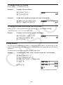
u To store a function
Example
To store the function (A+B) (A–B) as function memory number 1
!*( ( )a1(A-E)1(A)+
a2(B)!/( ) )
!*( ( )a1(A-E)1(A)a2(B)!/( ) )
K6(g)6(g)3(FMEM)
1(STO)bw
JJJ
• If the function memory number to which you store a function already contains a function, the
previous function is replaced with the new one.
• You can also use !K(→) to store a function in function
memory in a program. In this case, you must enclose the
function inside of double quotation marks.
u To recall a function
Example
To recall the contents of function memory number 1
AK6(g)6(g)3(FMEM)
2(RCL)bw
• The recalled function appears at the current location of the cursor on the display.
u To recall a function as a variable
Ad!K(→)a1(A-E)1(A)w
b!K(→)a1(A-E)2(B)w
K6(g)6(g)3(FMEM)3(fn)
b+cw
3-6
u To display a list of available functions
K6(g)6(g)3(FMEM)
4(SEE)
u To delete a function
Example
To delete the contents of function memory number 1
A
K6(g)6(g)3(FMEM)
1(STO)bw
• Executing the store operation while the display is blank deletes the function in the function
memory you specify.
k Answer Function
The Answer Function automatically stores the last result you calculated by pressing
w (unless the w key operation results in an error). The result is stored in the answer
memory.
• The largest value that the answer memory can hold is 15 digits for the mantissa and 2 digits
for the exponent.
• Answer memory contents are not cleared when you press the A key or when you switch
power off.
u To use the contents of the answer memory in a calculation
Example
123 + 456 = 579
789 – 579 = 210
Abcd+efgw
hij-Kw
3-7
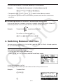
k Performing Continuous Calculations
Answer memory also lets you use the result of one calculation as one of the arguments in the
next calculation.
Example
1÷3=
1÷3×3=
Ab/dw
(Continuing)*dw
Continuous calculations can also be used with Type B functions (x2, x–1, x!, on page 3-2), +, –,
^(xy), x', ° ’ ”, etc.
3. Specifying the Angle Unit and Display Format
Before performing a calculation for the first time, you should use the Setup screen to specify
the angle unit and display format.
k Setting the Angle Unit
[SET UP]- [Angle]
1. On the Setup screen, highlight “Angle”.
2. Press the function key for the angle unit you want to specify, then press J.
• {Deg}/{Rad}/{Gra} ... {degrees}/{radians}/{grads}
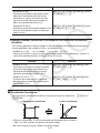
• The relationship between degrees, grads, and radians is shown below.
360° = 2π radians = 400 grads
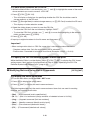
90° = π/2 radians = 100 grads
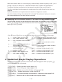
k Setting the Display Format
[SET UP]- [Display]
1. On the Setup screen, highlight “Display”.
2. Press the function key for the item you want to set, then press J.
• {Fix}/{Sci}/{Norm}/{Eng} ... {fixed number of decimal places specification}/
{number of significant digits specification}/{normal display}/{Engineering mode}
u To specify the number of decimal places (Fix)
Example
To specify two decimal places
1(Fix)cw
Press the number key that corresponds to the number of decimal places you want to specify
(n = 0 to 9).
• Displayed values are rounded off to the number of decimal places you specify.
3-8
u To specify the number of significant digits (Sci)
Example
To specify three significant digits
2(Sci)dw
Press the number key that corresponds to the number of significant digits you want to specify
(n = 0 to 9). Specifying 0 makes the number of significant digits 10.
• Displayed values are rounded off to the number of significant digits you specify.
u To specify the normal display (Norm 1/Norm 2)
Press 3(Norm) to switch between Norm 1 and Norm 2.
Norm 1: 10–2 (0.01) > |x|, |x| >1010
Norm 2: 10–9 (0.000000001) > |x|, |x| >1010
u To specify the engineering notation display (Eng mode)
Press 4(Eng) to switch between engineering notation and standard notation. The indicator
“/E” is on the display while engineering notation is in effect.
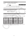
You can use the following symbols to convert values to engineering notation, such as 2,000
(= 2 × 103) → 2k.
E (Exa)
× 1018
m (milli)
× 10–3
P (Peta)
× 1015
μ (micro)
× 10–6
T (Tera)
× 1012
n (nano)
× 10–9
G (Giga)
× 109
p (pico)
× 10–12
M (Mega)
× 106
f (femto)
× 10–15
k (kilo)
× 103
• The engineering symbol that makes the mantissa a value from 1 to 1000 is automatically
selected by the calculator when engineering notation is in effect.
3-9
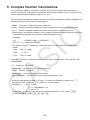
4. Function Calculations
k Function Menus
This calculator includes five function menus that give you access to scientific functions not
printed on the key panel.
• The contents of the function menu differ according to the mode you entered from the Main
Menu before you pressed the K key. The following examples show function menus that
appear in the RUN • MAT or PRGM mode.
u Hyperbolic Calculations (HYP)
[OPTN]-[HYP]
• {sinh}/{cosh}/{tanh} ... hyperbolic {sine}/{cosine}/{tangent}
• {sinh–1}/{cosh–1}/{tanh–1} ... inverse hyperbolic {sine}/{cosine}/{tangent}
u Probability/Distribution Calculations (PROB)
[OPTN]-[PROB]
• {x!} ... {press after inputting a value to obtain the factorial of the value}
• {nPr}/{nCr} ... {permutation}/{combination}
• {RAND} ... {random number generation}
• {Ran#}/{Int}/{Norm}/{Bin}/{List} ... {random number generation (0 to 1)}/{random integer
generation}/{random number generation in accordance with normal distribution based
on mean ƫ and standard deviation Ʊ}/{random number generation in accordance with
binomial distribution based on number of trials n and probability p}/{random number
generation (0 to 1) and storage of result in ListAns}
• {P(}/{Q(}/{R(} ... normal probability {P(t)}/{Q(t)}/{R(t)}
• {t(} ... {value of normalized variate t(x)}
u Numeric Calculations (NUM)
[OPTN]-[NUM]
• {Abs} ... {select this item and input a value to obtain the absolute value of the value}
• {Int}/{Frac} ... select the item and input a value to extract the {integer}/{fraction} part.
• {Rnd} ... {rounds off the value used for internal calculations to 10 significant digits (to match
the value in the answer memory), or to the number of decimal places (Fix) and number
of significant digits (Sci) specified by you}
• {Intg} ... {select this item and input a value to obtain the largest integer that is not greater
than the value}
• {RndFi} ... {rounds off the value used for internal calculations to specified digits (0 to 9) (see
page 3-2).}
• {GCD} ... {greatest common divisor for two values}
• {LCM} ... {least common multiple for two values}
• {MOD} ... {remainder of division (remainder output when n is divided by m)}
• {MOD • E} ... {remainder when division is performed on a power value (remainder output
when n is raised to p power and then divided by m)}
3-10
u Angle Units, Coordinate Conversion, Sexagesimal Operations (ANGL)
[OPTN]-[ANGL]
• {°}/{r}/{g} ... {degrees}/{radians}/{grads} for a specific input value
• {° ’ ”}* ... {specifies degrees (hours), minutes, seconds when inputting a degrees/minutes/
seconds value}
• {° ’ ”}* ... {converts decimal value to degrees/minutes/seconds value}
• The {° ’ ”} menu operation is available only when there is a calculation result on the display.
• {Pol(}/{Rec(}* ... {rectangular-to-polar}/{polar-to-rectangular} coordinate conversion
• {'DMS} ... {converts decimal value to sexagesimal value}
* These commands ({° ’ ”}, {° ’ ”}, {Pol(}, {Rec(}) can be input using key operations, without
going through the option (OPTN) menu. For operation examples, see “Angle Units” (page
3-11).
u Engineering Symbol (ESYM)
[OPTN]-[ESYM]
• {m}/{—}/{n}/{p}/{f} ... {milli (10–3)}/{micro (10–6)}/{nano (10–9)}/{pico (10–12)}/{femto (10–15)}
• {k}/{M}/{G}/{T}/{P}/{E} ... {kilo (103)}/{mega (106)}/{giga (109)}/{tera (1012)}/{peta (1015)}/
{exa (1018)}
• {ENG}/{ENG} ... shifts the decimal place of the displayed value three digits to the {left}/{right}
and {decreases}/{increases} the exponent by three.
When you are using engineering notation, the engineering symbol is also changed
accordingly.
• The {ENG} and {ENG} menu operations are available only when there is a calculation
result on the display.
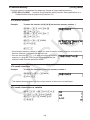
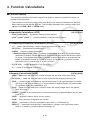
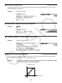
k Angle Units
• Be sure to specify Comp for Mode in the Setup screen.
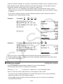
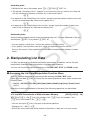
Example
Operation
47.3° + 82.5rad = 4774.20181°
47.3+82.5K6(g)5(ANGL)2(r)w
2°20´30˝ + 39´30˝ = 3°00´00˝
2$20$30$+0$39$30$w
!$(° ’ ”)
Convert 60° to radians.
1.047197551
!m(SET UP)cc2(Rad)J
60K6(g)5(ANGL)1(°)w
To convert 2.255 (decimal) to
sexagesimal
2°15’18”
2.255w!$(° ’ ”)
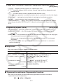
k Trigonometric and Inverse Trigonometric Functions
• Be sure to set the angle unit before performing trigonometric function and inverse
trigonometric function calculations.
(90° =
π
radians = 100 grads)
2
3-11
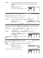
• Be sure to specify Comp for Mode in the Setup screen.
Example
Operation
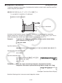
cos ( π rad) = 0.5
3
!m(SET UP)cc2(Rad)J!i(cos)
!*( ( )!a(CATALOG)a6(SYBL)4(9)
cc(π)w/3!/( ) )w
2 • sin 45° × cos 65° = 0.5976724775
!m(SET UP)cc1(Deg)J
2*!h(sin) 45*c65w*1
sin–10.5 = 30°
(x when sinx = 0.5)
!e(sin–1) 0.5*2w
*1 * can be omitted.
*2 Input of leading zero is not necessary.
k Logarithmic and Exponential Functions
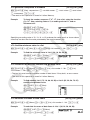
• Be sure to specify Comp for Mode in the Setup screen.
Example
Operation
log 1.23 (log101.23) = 0.08990511144 !a(CATALOG)a3(K-O)2(L)c~c(log)
w1.23w
log28 = 3
K4(CALC)6(g)4(logab) 2,8
!/( ) )w
(–3)4 = (–3) × (–3) × (–3) × (–3) = 81
!*( ( )-3!/( ) )!a(CATALOG)
a6(SYBL)4(9)c~c(^)w 4w
7
1
123 (= 123 7 ) = 1.988647795
7!a(CATALOG)a6(SYBL)4(9)c~c
(x')w 123w
k Hyperbolic and Inverse Hyperbolic Functions
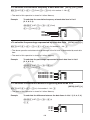
• Be sure to specify Comp for Mode in the Setup screen.
Example
sinh 3.6 = 18.28545536
cosh–1
20
= 0.7953654612
15
Operation
K6(g)2(HYP)1(sinh) 3.6w
K6(g)2(HYP)5(cosh–1)!*( ( ) 20/15
!/( ) )w
3-12
k Other Functions
• Be sure to specify Comp for Mode in the Setup screen.
Example
Operation
'
2 +'
5 = 3.65028154
!x(') 2+!x(') 5w
(–3)2 = (–3) × (–3) = 9
!*( ( )-3!/( ) )xw
8! (= 1 × 2 × 3 × .... × 8) = 40320
8K6(g)3(PROB)1(x!)w
What is the integer part of – 3.5?
K6(g)4(NUM)2(Int)-3.5w
–3
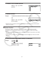
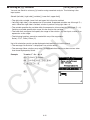
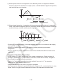
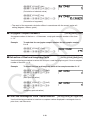
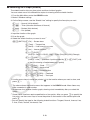
k Random Number Generation (RAND)
u Random Number Generation (0 to 1) (Ran#, RanList#)
Ran# and RanList# generate 10 digit random numbers randomly or sequentially from 0 to 1.
Ran# returns a single random number, while RanList# returns multiple random numbers in list
form. The following shows the syntaxes of Ran# and RanList#.
Ran# [a]
1<a<9
RanList# (n [,a])
1 < n < 999
• n is the number of trials. RanList# generates the number of random numbers that
corresponds to n and displays them on the ListAns screen. A value must be input for n.
• “a” is the randomization sequence. Random numbers are returned if nothing is input for “a”.
Entering an integer of 1 through 9 for a will return the corresponding sequential random
number.
• Executing the function Ran# 0 initializes the sequences of both Ran# and RanList#. The
sequence also is initialized when a sequential random number is generated with a different
sequence of the previous execution using Ran# or RanList#, or when generating a random
number.
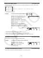
Ran# Examples
Example
Operation
K6(g)3(PROB)4(RAND)
1(Ran#)w
Ran#
(Generates a random number.)
(Each press of w generates a new random number.)
w
w
Ran# 1
(Generates the first random number in sequence 1.)
K6(g)3(PROB)4(RAND)
1(Ran#) 1w
(Generates the second random number in sequence 1.)
w
Ran# 0
(Initializes the sequence.)
1(Ran#) 0w
Ran# 1
(Generates the first random number in sequence 1.)
1(Ran#) 1w
3-13
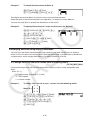
RanList# Examples
Example
Operation
RanList# (4)
(Generates four random numbers and
displays the result on the ListAns screen.)
K6(g)3(PROB)4(RAND)5(List)
4!/( ) )w
RanList# (3, 1)
(Generates from the first to the third random
numbers of sequence 1 and displays the
result on the ListAns screen.)
JK6(g)3(PROB)4(RAND)
5(List) 3,1!/( ) )w
(Next, generates from the fourth to the sixth
random number of sequence 1 and displays
the result on the ListAns screen.)
Jw
Ran# 0
(Initializes the sequence.)
J1(Ran#) 0w
RanList# (3, 1)
5(List) 3,1!/( ) )w
(Re-generates from the first to the third
random numbers of sequence 1 and displays
the result on the ListAns screen.)
u Random Integer Generation (RanInt#)
RanInt# generates random integers that fall between two specified integers.
RanInt# (A, B [,n])
A<B
|A|,|B| < 1E10
B – A < 1E10
1 < n < 999
• A is the start value and B is the end value. Omitting a value for n returns a generated random
number as-is. Specifying a value for n returns the specified number of random values in list
form.
Example
Operation
RanInt# (1, 5)
(Generates one random integer from 1 and
5.)
K6(g)3(PROB)4(RAND)2(Int)
1,5!/( ) )w
RanInt# (1, 10, 5)
(Generates five random integers from 1 to
10 and displays the result on the ListAns
screen.)
K6(g)3(PROB)4(RAND)2(Int)
1,10,5!/( ) )w
u Random Number Generation in Accordance with Normal Distribution
(RanNorm#)
This function generates a 10-digit random number in accordance with normal distribution
based on a specified mean ƫ and standard deviation Ʊ values.
RanNorm# (Ʊ, ƫ [,n])
Ʊ>0
1 < n < 999
• Omitting a value for n returns a generated random number as-is. Specifying a value for n
returns the specified number of random values in list form.
3-14
Example
Operation
RanNorm# (8, 68)
(Randomly produces a body length value
obtained in accordance with the normal
distribution of a group of infants less than
one year old with a mean body length of
68cm and standard deviation of 8.)
K6(g)3(PROB)4(RAND)3(Norm)
8,68!/( ) )w
RanNorm# (8, 68, 5)
(Randomly produces the body lengths of five
infants in the above example, and displays
them in a list.)
K6(g)3(PROB)4(RAND)3(Norm)
8,68,5!/( ) )w
u Random Number Generation in Accordance with Binomial Distribution
(RanBin#)
This function generates random integers in accordance with binomial distribution based on
values specified for the number of trials n and probability p.
RanBin# (n, p [,m])
1 < n < 100000
1 < m < 999
0<p<1
• Omitting a value for m returns a generated random number as-is. Specifying a value for m
returns the specified number of random values in list form.
Example
Operation
RanBin# (5, 0.5)
(Randomly produces the number of heads
that can be expected in accordance with
binomial distribution for five coin tosses
where the probability of heads is 0.5.)
K6(g)3(PROB)4(RAND)4(Bin)
5,0.5!/( ) )w
RanBin# (5, 0.5, 3)
(Performs the same coin toss sequence
described above three times and displays
the results in a list.)
K6(g)3(PROB)4(RAND)4(Bin)
5,0.5,3!/( ) )w
k Coordinate Conversion
You can perform coordinate conversion using the following key operations: !-(Pol) or
!+(Rec).
u Rectangular Coordinates
u Polar Coordinates
• With polar coordinates, Ƨ can be calculated and displayed within a range of
–180°< Ƨ < 180° (radians and grads have same range).
• Be sure to specify Comp for Mode in the Setup screen.
3-15
Example
Operation
1 Calculate r and Ƨ° when x = 14 and y = 20.7
!m(SET UP)cc1(Deg)J
!-(Pol) 14,20.7!/( ) )wJ
1
2
24.989
55.928
→
→
24.98979792 (r)
55.92839019 (θ )
2 Calculate x and y when r = 25 and Ƨ = 56°
1
2
13.979
20.725
→
→
!+(Rec) 25,56!/( ) )w
13.97982259 (x)
20.72593931 (y)
• The results of coordinate conversions are automatically stored in ListAns Memory.
Example 1 result
Example 2 result
k Permutation and Combination
u Permutation
n!
nPr =
(n – r)!
u Combination
n!
nCr =
r! (n – r)!
• Be sure to specify Comp for Mode in the Setup screen.
Example 1
To calculate the possible number of different arrangements using 4
items selected from among 10 items
Formula
P4 = 5040
10K6(g)3(PROB)2(nPr) 4w
10
Example 2
Operation
To calculate the possible number of different combinations of 4 items
that can be selected from among 10 items
Formula
C4 = 210
Operation
10K6(g)3(PROB)3(nCr) 4w
10
k Greatest Common Divisor (GCD), Least Common Multiple (LCM)
Example
Operation
To determine the greatest common
divisor of 28 and 35
(GCD (28, 35) = 7)
K6(g)4(NUM)6(g)2(GCD) 28,
35!/( ) )w
To determine the least common multiple
of 9 and 15
(LCM (9, 15) = 45)
K6(g)4(NUM)6(g)3(LCM) 9,15
!/( ) )w
3-16
k Division Remainder (MOD), Remainder of Exponential Division (MOD
Exp)
Example
Operation
To determine the remainder when 137 is
divided by 7
(MOD (137, 7) = 4)
K6(g)4(NUM)6(g)4(MOD) 137,7
!/( ) )w
To determine the remainder when 53 is
divided by 3
(MOD • E (5, 3, 3) = 2)
K6(g)4(NUM)6(g)5(MOD • E)
5,3,3!/( ) )w
k Fractions
• Be sure to specify Comp for Mode in the Setup screen.
Example
Operation
2
1
73
–– + 3 –– = –––
5
4
20
2!a(CATALOG)a6(SYBL)4(9)c~
c({)w5+3!a(CATALOG)({)
1(INPUT)1!a(CATALOG)({)1(INPUT)
4w
1
1
––––– + ––––– = 6.066202547 × 10–4 *1
2578
4572
1!a(CATALOG)a6(SYBL)4(9)c~
c({)w2578+1!a(CATALOG)({)
1(INPUT)4572w
1
–– × 0.5 = 0.25*2
2
1!a(CATALOG)a6(SYBL)4(9)c~
c({)w2*.5w
*1 When the total number of characters, including integer, numerator, denominator and delimiter
marks exceeds 10, the fraction is automatically displayed in decimal format.
*2 Calculations containing both fractions and decimals are calculated in decimal format.
k Engineering Notation Calculations
Input engineering symbols using the engineering notation menu.
• Be sure to specify Comp for Mode in the Setup screen.
Example
Operation
999k (kilo) + 25k (kilo)
= 1.024M (mega)
!m(SET UP)ff4(Eng)J999K6(g)6(g)
1(ESYM)6(g)1(k)+251(k)w
9 ÷ 10 = 0.9 = 900m (milli)
= 0.9
9/10w
K6(g)6(g)1(ESYM)6(g)6(g)3(ENG)*1
= 0.0009k (kilo)
= 0.9
= 900m
3(ENG)*1
2(ENG)*2
2(ENG)*2
3-17
*1 Converts the displayed value to the next higher engineering unit, by shifting the decimal
point three places to the right.
*2 Converts the displayed value to the next lower engineering unit, by shifting the decimal point
three places to the left.
k Logical Operators (AND, OR, NOT, XOR)
[OPTN]-[LOGIC]
The logical operator menu provides a selection of logical operators.
• {And}/{Or}/{Not}/{Xor} ... {logical AND}/{logical OR}/{logical NOT}/{logical XOR}
• Be sure to specify Comp for Mode in the Setup screen.
Example
What is the logical AND of A and B when A = 3 and B = 2?
A AND B = 1
Operation
Display
3!K(→)a1(A-E)1(A)w
2!K(→)a1(A-E)2(B)w
1(A)K6(g)6(g)4(LOGIC)
1(And)a1(A-E)2(B)w
1
u About Logical Operations
• A logical operation always produces either 0 or 1 as its result.
• The following table shows all of possible results that can be produced by AND, OR and XOR
operations.
Value or Expression A
Value or Expression B
A AND B
A OR B
A XOR B
A≠0
B≠0
1
1
0
A≠0
B=0
0
1
1
A=0
B≠0
0
1
1
A=0
B=0
0
0
0
• The following table shows the results produced by the NOT operation.
Value or Expression A
NOT A
A≠0
0
A=0
1
3-18
5. Numerical Calculations
The following explains the numerical calculation operations included in the function menu
displayed when K4(CALC) is pressed. The following calculations can be performed.
• {Int÷}/{Rmdr}/{Simp} ... {quotient}/{remainder}/{simplification}
• {Solve}/{d/dx}/{d2/dx2}/{∫dx}/{SolvN} ... {equality solution}/{differential}/{quadratic differential}/
{integration}/{f(x) function solution}
• {FMin}/{FMax}/{Σ(}/{logab} ... {minimum value}/{maximum value}/{summation}/{logarithm
logab}
k Quotient of Integer ÷ Integer
[OPTN]-[CALC]-[Int÷]
The “Int÷” function can be used to determine the quotient when one integer is divided by
another integer.
Example
To calculate the quotient of 107 ÷ 7
AbahK4(CALC)6(g)
6(g)1(Int÷)h
w
k Remainder of Integer ÷ Integer
[OPTN]-[CALC]-[Rmdr]
The “Rmdr” function can be used to determine the remainder when one integer is divided by
another integer.
Example
To calculate the remainder of 107 ÷ 7
AbahK4(CALC)6(g)
6(g)2(Rmdr)h
w
k Simplification
[OPTN]-[CALC]-[Simp]
The “'Simp” function can be used to simplify fractions manually. The following operations can
be used to perform simplification when an unsimplified calculation result is on the display.
• {Simp} w ... This function automatically simplifies the displayed calculation result using the
smallest prime number available. The prime number used and the simplified result are
shown on the display.
• {Simp} n w ... This function performs simplification according to the specified divisor n.
3-19
Under initial default settings, this calculator automatically simplifies fraction calculation results
before displaying them. Before performing the following examples, use the Setup screen to
change the “Simplify” setting from “Auto” to “Manual” (page 2-15).
• When “a+bi” or “r∠θ” is specified for the Setup screen “Complex Mode” setting, fraction
calculation results always are simplified before being displayed, even if the “Simplify” setting
is “Manual”.
• If you want to simplify fractions manually (Simplify: Manual), make sure that the “Real” is
selected for the “Complex Mode” setting.
Example 1
15
60
To simplify
5
1
15
=
=
4
60 20
Abf!a(CATALOG)
a6(SYBL)4(9)c~c({)w
gawK4(CALC)6(g)6(g)
3(Simp)w
3(Simp)w
The “F=” value is the divisor.
Example 2
To simplify
27
specifying a divisor of 9
63
3
27
=
7
63
Ach!a(CATALOG)
a6(SYBL)4(9)c~c({)w
gdwK4(CALC)6(g)6(g)
3(Simp)jw
• An error occurs if simplification cannot be performed using the specified divisor.
• Executing 'Simp while a value that cannot be simplified is displayed will return the original
value, without displaying “F=”.
k Solve Calculations
[OPTN]-[CALC]-[Solve]
SOLVE uses approximation based on Newton’s Law to solve equations.
The following is the syntax for using the Solve function.
Solve( f(x), n, a, b)
(a: lower limit, b: upper limit, n: initial estimated value)
An error (Time Out) occurs when there is no convergence of the solution.
• You cannot use a quadratic differential, Σ, maximum/minimum value or Solve calculation
expression inside of any of the above functions.
• Pressing A during calculation of Solve (while the cursor is not shown on the display)
interrupts the calculation.
3-20
k Solving an f(x) Function
[OPTN]-[CALC]-[SolvN]
You can use SolvN to solve an f(x) function using numerical analysis. The following is the
input syntax.
SolveN (left side [=right side] [,variable] [, lower limit, upper limit])
• The right side, variable, lower limit and upper limit all can be omitted.
• “left side[=right side]” is the expression to be solved. Supported variables are A through Z, r,
and θ. When the right side is omitted, solution is perform using right side = 0.
• The variable specifies the variable within the expression to be solved for (A through Z, r, θ).
Omitting a variable specification cause X to be used as the variable.
• The lower limit and upper limit specify the range of the solution. You can input a value or an
expression as the range.
• The following functions cannot be used within any of the arguments.
Solve(, d2/dx2, FMin(, FMax(, Σ(
Up to 10 calculation results can be displayed simultaneously in ListAns format.
• The message “No Solution” is displayed if no solution exists.
• The message “More solutions may exist.” is displayed when there may be solutions other
than those displayed by SolvN.
Example
To solve x2 – 5x – 6 = 0
K4(CALC)5(SolvN)
a5(U-Z)4(X)x-f4(X)
-g!/( ) )w
J
3-21
k Differential Calculations
[OPTN]-[CALC]-[d/dx]
To perform differential calculations, first display the function analysis menu, and then input the
values using the syntax below.
K4(CALC)2(d/dx) f(x),a,tol!/( ) )
(a: point for which you want to determine the derivative, tol: tolerance)
d f (a)
d/dx ( f (x), a) ⇒
dx
The differentiation for this type of calculation is defined as:
f (a + Ax) – f (a)
f ' (a) = lim –––––––––––––
Ax→0
Ax
In this definition, infinitesimal is replaced by a sufficiently small Ax, with the value in the
neighborhood of f' (a) calculated as:
f (a + Ax) – f (a)
f ' (a) –––––––––––––
Ax
In order to provide the best precision possible, this unit employs central difference to perform
differential calculations.
Example
To determine the derivative at point x = 3 for the function
y = x3 + 4x2 + x – 6, with a tolerance of “tol” = 1E – 5
Input the function f(x).
AK4(CALC)2(d/dx)a5(U-Z)4(X)!a(CATALOG)
a6(SYBL)4(9)c~c(^)wd+ea5(U-Z)4(X)
x+4(X)-g,
Input point x = a for which you want to determine the derivative.
d,
Input the tolerance value.
b!a(CATALOG)a1(A-E)5(E)
c~c(EXP)w-f!/( ) )w
Differential Calculation Precautions
• In the function f(x), only X can be used as a variable in expressions. Other variables
(A through Z excluding X, r, Ƨ) are treated as constants, and the value currently assigned to
that variable is applied during the calculation.
• Input of the tolerance (tol) value and the closing parenthesis can be omitted. If you omit
tolerance (tol) value, the calculator automatically uses a value for tol as 1E–10.
• Specify a tolerance (tol) value of 1E–14 or greater. An error (Time Out) occurs whenever no
solution that satisfies the tolerance value can be obtained.
• Pressing A during calculation of a differential (while the cursor is not shown on the display)
interrupts the calculation.
• Inaccurate results and errors can be caused by the following:
- discontinuous points in x values
- extreme changes in x values
- inclusion of the local maximum point and local minimum point in x values
3-22
- inclusion of the inflection point in x values
- inclusion of undifferentiable points in x values
- differential calculation results approaching zero
• Always use radians (Rad mode) as the angle unit when performing trigonometric
differentials.
• You cannot use a differential, quadratic differential, integration, Σ, maximum/minimum value,
Solve, RndFix or logab calculation expression inside a differential calculation term.
k Quadratic Differential Calculations
[OPTN]-[CALC]-[d2/dx2]
After displaying the function analysis menu, you can input quadratic differentials using the
following syntax.
K4(CALC)3(d2/dx2) f(x),a,tol!/( ) )
(a: differential coefficient point, tol: tolerance)
Quadratic differential calculations produce an approximate differential value using the following
second order differential formula, which is based on Newton’s polynomial interpretation.
In this expression, values for “sufficiently small increments of h” are used to obtain a value that
approximates f"(a).
Example
To determine the quadratic differential coefficient at the point where
x = 3 for the function y = x3 + 4x2 + x – 6
Here we will use a tolerance tol = 1E – 5
Input the function f(x).
AK4(CALC)3(d2/dx2)a5(U-Z)4(X)!a(CATALOG)
a6(SYBL)4(9)c~c(^)wd+ea5(U-Z)4(X)
x+4(X)-g,
Input 3 as point a, which is the differential coefficient point.
d,
Input the tolerance value.
b!a(CATALOG)a1(A-E)
5(E)c~c(EXP)w
-f!/( ) )
w
Quadratic Differential Calculation Precautions
• With quadratic differential calculation, calculation precision is up to five digits for the
mantissa.
• The rules that apply for linear differential also apply when using a quadratic differential
calculation. See “Differential Calculation Precautions” on page 3-22.
3-23
[OPTN]-[CALC]-[∫dx]
k Integration Calculations
To perform integration calculations, first display the function analysis menu and then input the
values using the syntax below.
K4(CALC)4(∫dx) f(x) , a , b , tol !/( ) )
(a: start point, b: end point, tol: tolerance)
∫( f(x), a, b, tol) ⇒ ∫a f(x)dx
b
Area of
∫
b
a
f(x)dx is calculated
As shown in the illustration above, integration calculations are performed by calculating
integral values from a through b for the function y = f (x) where a < x < b, and f (x) > 0. This in
effect calculates the surface area of the shaded area in the illustration.
Example 1
To perform the integration calculation for the function shown below,
with a tolerance of “tol” = 1E – 4
∫
5
1
(2x2 + 3x + 4) dx
Input the function f (x).
AK4(CALC)4(∫dx)ca5(U-Z)4(X)x+d4(X)+e,
Input the start point and end point.
b,f,
Input the tolerance value.
b!a(CATALOG)a1(A-E)5(E)
c~c(EXP)w-e
!/( ) )w
Example 2
When the angle unit setting is degrees, trigonometric function
integration calculation is performed using radians (Angle unit = Deg)
Examples Calculation Result Display
Note the following points to ensure correct integration values.
3-24
(1) When cyclical functions for integration values become positive or negative for different
divisions, perform the calculation for single cycles, or divide between negative and positive,
and then add the results together.
Positive
part (S )
Negative part (S )
∫
b
a
f(x)dx =
∫
c
a
f(x)dx +
Positive part (S)
∫
b
c
f(x)dx
Negative part (S)
(2) When minute fluctuations in integration divisions produce large fluctuations in integration
values, calculate the integration divisions separately (divide the large fluctuation areas into
smaller divisions), and then add the results together.
∫
b
a
f(x)dx =
∫
x
a
1
f(x)dx +
∫
x
2
x
f(x)dx +.....+
1
∫
b
x
f(x)dx
4
• Pressing A during calculation of an integral (while the cursor is not shown on the display)
interrupts the calculation.
• Always use radians (Rad mode) as the angle unit when performing trigonometric
integrations.
• An error (Time Out) occurs whenever no solution that satisfies the tolerance value can be
obtained.
Integration Calculation Precautions
• In the function f(x), only X can be used as a variable in expressions. Other variables (A
through Z excluding X, r, Ƨ) are treated as constants, and the value currently assigned to
that variable is applied during the calculation.
• Input of “tol” and closing parenthesis can be omitted. If you omit “tol,” the calculator
automatically uses a default value of 1E–5.
• Integration calculations can take a long time to complete.
• You cannot use a differential, quadratic differential, integration, Σ, maximum/minimum value,
Solve, RndFix or logab calculation expression inside of an integration calculation term.
3-25
k Σ Calculations
[OPTN]-[CALC]-[Σ(]
To perform Σ calculations, first display the function analysis menu, and then input the values
using the syntax below.
K4(CALC)6(g)3(Σ( ) ak , k , α , β , n !/( ) )
β
Σ (a , k, α, β, n) = Σ a = a
k
k
k=α
α
+ aα +1 +........+ aβ
(n: distance between partitions)
Example
To calculate the following:
6
Σ (k
2
– 3k + 5)
k=2
Use n = 1 as the distance between partitions.
AK4(CALC)6(g)3(Σ( )
a3(K-O)1(K)x-d1(K)
+f,1(K),c,g,b
!/( ) )w
Σ Calculation Precautions
• The value of the specified variable changes during a Σ calculation. Be sure to keep separate
written records of the specified variable values you might need later before you perform the
calculation.
• You can use only one variable in the function for input sequence ak.
• Input integers only for the initial term (α) of sequence ak and last term (β) of sequence ak.
• Input of n and the closing parentheses can be omitted. If you omit n, the calculator
automatically uses n = 1.
• Make sure that the value used as the final term β is greater than the value used as the initial
term α. Otherwise, an error will occur.
• To interrupt an ongoing Σ calculation (indicated when the cursor is not on the display), press
the A key.
• You cannot use a differential, quadratic differential, integration, Σ, maximum/minimum value,
Solve, RndFix or logab calculation expression inside of a Σ calculation term.
k Maximum/Minimum Value Calculations
[OPTN]-[CALC]-[FMin]/[FMax]
After displaying the function analysis menu, you can input maximum/minimum calculations
using the formats below, and solve for the maximum and minimum of a function within interval
a < x < b.
u Minimum Value
K4(CALC)6(g)1(FMin) f (x) , a , b , n !/( ) )
(a: start point of interval, b: end point of interval, n: precision (n = 1 to 9))
3-26
u Maximum Value
K4(CALC)6(g)2(FMax) f (x), a , b , n !/( ) )
(a: start point of interval, b: end point of interval, n: precision (n = 1 to 9))
Example
To determine the minimum value for the interval defined by start
point a = 0 and end point b = 3, with a precision of n = 6 for the function
y = x2 – 4x + 9
Input f (x).
AK4(CALC)6(g)1(FMin)a5(U-Z)4(X)x-e4(X)
+j,
Input the interval a = 0, b = 3.
a,d,
Input the precision n = 6.
g!/( ) )w
• In the function f (x), only X can be used as a variable in expressions. Other variables (A
through Z excluding X, r, Ƨ) are treated as constants, and the value currently assigned to
that variable is applied during the calculation.
• Input of n and the closing parenthesis can be omitted.
• Discontinuous points or sections with drastic fluctuation can adversely affect precision or
even cause an error.
• Inputting a larger value for n increases the precision of the calculation, but it also increases
the amount of time required to perform the calculation.
• The value you input for the end point of the interval (b) must be greater than the value you
input for the start point (a). Otherwise an error occurs.
• You can interrupt an ongoing maximum/minimum calculation by pressing the A key.
• You can input an integer in the range of 1 to 9 for the value of n. Using any value outside this
range causes an error.
• You cannot use a differential, quadratic differential, integration, Σ, maximum/minimum value,
Solve, RndFix or logab calculation expression inside of a maximum/minimum calculation
term.
3-27
6. Complex Number Calculations
You can perform addition, subtraction, multiplication, division, parentheses calculations,
function calculations, and memory calculations with complex numbers just as you do with the
manual calculations described on pages 3-1 to 3-13.
You can select the complex number calculation mode by changing the Complex Mode item on
the Setup screen to one of the following settings.
• {Real} ... Calculation in the real number range only*1
• {a+bi} ... Performs complex number calculation and displays results in rectangular form
• {r∠Ƨ} ... Performs complex number calculation and displays results in polar form*2
*1 When there is an imaginary number in the argument, however, complex number calculation
is performed and the result is displayed using rectangular form.
Examples:
ln 2i
= 0.6931471806 + 1.570796327i
ln 2i + ln (– 2) = (Non-Real ERROR)
*2 The display range of Ƨ depends on the angle unit set for the Angle item on the Setup
screen.
• Deg ... –180 < Ƨ < 180
• Rad ... – π < Ƨ < π
• Gra ... –200 < Ƨ < 200
Press K3(CPLX) to display the complex calculation number menu, which contains the
following items.
• {i} ... {imaginary unit i input}
• {Abs}/{Arg} ... obtains {absolute value}/{argument}
• {Conj} ... {obtains conjugate}
• {ReP}/{ImP} ... {real}/{imaginary} part extraction
• {'r∠Ƨ}/{'a+bi} ... converts the result to {polar}/{rectangular} form
• Solutions obtained by the Real, a+bi and r∠Ƨ modes are different for power root (x')
calculations when x < 0 and y = m/n when n is an odd number.
Example: 3x' (– 8) = – 2 (Real)
= 1 + 1.732050808i (a +bi)
= 2∠60 (r ∠Ƨ )
• To input the “ ∠ ” operator into the polar coordinate expression (r ∠Ƨ ), press !a
(CATALOG)a6(SYBL)4(9)c~c(∠)w.
3-28
k Arithmetic Operations
[OPTN]-[CPLX]-[i]
Arithmetic operations are the same as those you use for manual calculations. You can even
use parentheses and memory.
Example
(1 + 2i) + (2 + 3i)
AK3(CPLX)
!*( ( )b+c1(i)!/( ) )
+!*( ( )c+d1(i)
!/( ) )w
k Reciprocals, Square Roots, and Squares
Example
(3 + i)
AK3(CPLX)
!x(')!*( ( )d+
1(i)!/( ) )w
k Complex Number Format Using Polar Form
Example
2∠30 × 3∠45 = 6∠75
!m(SET UP)cc1(Deg)c
3(r∠Ƨ)J
Ac!a(CATALOG)a6(SYBL)
4(9)c~c(∠)wda*d
!a(CATALOG) (∠)1(INPUT)efw
k Absolute Value and Argument
[OPTN]-[CPLX]-[Abs]/[Arg]
The unit regards a complex number in the form a + bi as a coordinate on a Gaussian plane,
and calculates absolute value⎮Z ⎮and argument (arg).
Example
To calculate absolute value (r) and argument (Ƨ) for the complex number
3 + 4i, with the angle unit set for degrees
Imaginary axis
Real axis
3-29
AK3(CPLX)2(Abs)
!*( ( )d+e1(i)!/( ) )w
(Calculation of absolute value)
AK3(CPLX)3(Arg)
!*( ( )d+e1(i)!/( ) )w
(Calculation of argument)
• The result of the argument calculation differs in accordance with the current angle unit
setting (degrees, radians, grads).
k Conjugate Complex Numbers
[OPTN]-[CPLX]-[Conj]
A complex number of the form a + bi becomes a conjugate complex number of the form
a – bi.
Example
To calculate the conjugate complex number for the complex number
2 + 4i
AK3(CPLX)4(Conj)
!*( ( )c+e1(i)!/( ) )w
k Extraction of Real and Imaginary Parts
[OPTN]-[CPLX]-[ReP]/[lmP]
Use the following procedure to extract the real part a and the imaginary part b from a complex
number of the form a + bi.
Example
To extract the real and imaginary parts of the complex number 2 + 5i
AK3(CPLX)6(g)1(ReP)
!*( ( )c+f6(g)1(i)
!/( ) )w
(Real part extraction)
AK3(CPLX)6(g)2(ImP)
!*( ( )c+f6(g)1(i)
!/( ) )w
(Imaginary part extraction)
k Polar and Rectangular Form Transformation
[OPTN]-[CPLX]-['r∠Ƨ]/['a+bi]
Use the following procedure to transform a complex number displayed in rectangular form to
polar form, and vice versa.
3-30
Example
To transform the rectangular form of complex number 1 + '
3 i to its
polar form
!m(SET UP)cc1(Deg)c
2(a+bi)J
Ab+!*( ( )!x(')d
!/( ) )K3(CPLX)
1(i)6(g)3('r∠θ)w
Ac!a(CATALOG)a6(SYBL)
4(9)c~c(∠)wgaK3(CPLX)
6(g)4('a+bi)w
• The input/output range of complex numbers is normally 10 digits for the mantissa and two
digits for the exponent.
• When a complex number has more than 21 digits, the real part and imaginary part are
displayed on separate lines.
• The following functions can be used with complex numbers.
', x 2, x –1, ^(x y), 3', x', In, log, logab, 10x, e x, Int, Frac, Rnd, Intg, RndFix(, Fix, Sci, ENG,
ENG, ° ’ ”, ° ’ ”, a b/c, d /c
7. Binary, Octal, Decimal, and Hexadecimal
Calculations with Integers
You can use the RUN • MAT mode and binary, octal, decimal, and hexadecimal settings to
perform calculations that involve binary, octal, decimal and hexadecimal values. You can also
convert between number systems and perform bitwise operations.
• You cannot use scientific functions in binary, octal, decimal, and hexadecimal calculations.
• You can use only integers in binary, octal, decimal, and hexadecimal calculations, which
means that fractional values are not allowed. If you input a value that includes a decimal
part, the calculator automatically cuts off the decimal part.
• If you attempt to enter a value that is invalid for the number system (binary, octal, decimal,
hexadecimal) you are using, the calculator displays an error message. The following shows
the numerals that can be used in each number system.
Binary: 0, 1
Octal: 0, 1, 2, 3, 4, 5, 6, 7
Decimal: 0, 1, 2, 3, 4, 5, 6, 7, 8, 9
Hexadecimal: 0, 1, 2, 3, 4, 5, 6, 7, 8, 9, A, B, C, D, E, F
• Negative binary, octal, and hexadecimal values are produced using the two’s complement of
the original value.
• The following are the display capacities for each of the number systems.
Number System
Binary
Octal
Decimal
Hexadecimal
Display Capacity
16 digits
11 digits
10 digits
8 digits
3-31
• The alphabetic characters used in the hexadecimal number appear differently on the display
to distinguish them from text characters.
Normal Text
A
B
C
D
E
F
Hexadecimal
Values
u
v
w
x
y
z
4(HEX)
1(A)
4(HEX)
2(B)
4(HEX)
3(C)
4(HEX)
4(D)
4(HEX)
5(E)
4(HEX)
6(F)
Keys
• The following are the calculation ranges for each of the number systems.
Binary Values
Positive: 0 < x < 111111111111111
Negative: 1000000000000000 < x < 1111111111111111
Octal Values
Positive: 0 < x < 17777777777
Negative: 20000000000 < x < 37777777777
Decimal Values
Positive: 0 < x < 2147483647
Negative: –2147483648 < x < –1
Hexadecimal Values
Positive: 0 < x < 7FFFFFFF
Negative: 80000000 < x < FFFFFFFF
u To perform a binary, octal, decimal, or hexadecimal calculation
[SET UP]-[Mode]-[Dec]/[Hex]/[Bin]/[Oct]
1. In the Main Menu, select RUN • MAT.
2. Press !m(SET UP). Move the highlighting to “Mode”, and then specify the default
number system by pressing 2(Dec), 3(Hex), 4(Bin), or 5(Oct) for the Mode setting.
3. Press J to change to the screen for calculation input. This causes a function menu with
the following items to appear.
• {d~o}/{LOG}/{DISP}/{HEX} ... {number system specification}/{bitwise operation}/
{decimal/hexadecimal/binary/octal conversion}/{hexadecimal letter (A through F)
input} menu
k Selecting a Number System
You can specify decimal, hexadecimal, binary, or octal as the default number system using the
Setup screen.
u To specify a number system for an input value
You can specify a number system for each individual value you input. Press 1(d~o) to
display a menu of number system symbols. Press the function key that corresponds to the
symbol you want to select and then input the value.
• {d}/{h}/{b}/{o} ... {decimal}/{hexadecimal}/{binary}/{octal}
3-32
u To input values of mixed number systems
Example
To input 12310, when the default number system is hexadecimal
!m(SET UP)
Move the highlighting to “Mode”, and then
press 3(Hex)J.
A1(d~o)1(d)bcdw
k Negative Values and Bitwise Operations
Press 2(LOG) to display a menu of negation and bitwise operators.
• {Neg} ... {negation}*1
• {Not}/{and}/{or}/{xor}/{xnor} ... {NOT}*2/{AND}/{OR}/{XOR}/{XNOR}*3
*1 two’s complement
*2 one’s complement (bitwise complement)
*3 bitwise AND, bitwise OR, bitwise XOR, bitwise XNOR
u Negative Values
Example
To determine the negative of 1100102
!m(SET UP)
Move the highlighting to “Mode”, and then
press 4(Bin)J.
A2(LOG)1(Neg)
bbaabaw
• Negative binary, octal, and hexadecimal values are produced by taking the binary two’s
complement and then returning the result to the original number base. With the decimal
number base, negative values are displayed with a minus sign.
u Bitwise Operations
Example
To input and execute “12016 and AD16”
!m(SET UP)
Move the highlighting to “Mode”, and then
press 3(Hex)J.
Abca2(LOG)
3(and)J4(HEX)1(A)4(D)w
k Number System Transformation
Press 3(DISP) to display a menu of number system transformation functions.
• {'Dec}/{'Hex}/{'Bin}/{'Oct} ... transformation of displayed value to its {decimal}/
{hexadecimal}/{binary}/{octal} equivalent
3-33
u To convert a displayed value from one number system to another
Example
To convert 2210 (default number system) to its binary or octal value
A!m(SET UP)
Move the highlighting to “Mode”, and then
press 2(Dec)J.
1(d~o)1(d)ccw
J3(DISP)3('Bin)w
4('Oct)w
8. Matrix Calculations
From the Main Menu, enter the RUN • MAT mode, and press 1('MAT) to perform Matrix
calculations.
26 matrix memories (Mat A through Mat Z) plus a Matrix Answer Memory (MatAns), make it
possible to perform the following matrix operations.
• Addition, subtraction, multiplication, division
• Scalar multiplication calculations
• Determinant calculations
• Matrix transposition
• Matrix inversion
• Matrix squaring
• Raising a matrix to a specific power
• Absolute value, integer part extraction, fractional part extraction, maximum integer
calculations
• Inputting complex numbers in matrix elements and using complex number related functions
• Matrix modification using matrix commands
The maximum number of rows that can be specified for a matrix is 999, and the maximum
number of columns is 999.
About Matrix Answer Memory (MatAns)
• The calculator automatically stores matrix calculation results in Matrix Answer Memory. Note
the following points about Matrix Answer Memory.
• Whenever you perform a matrix calculation, the current Matrix Answer Memory contents are
replaced by the new result. The previous contents are deleted and cannot be recovered.
• Inputting values into a matrix does not affect Matrix Answer Memory contents.
3-34
k Inputting and Editing Matrices
Pressing 1('MAT) displays the Matrix Editor screen. Use the Matrix Editor to input and edit
matrices.
m × n … m (row) × n (column) matrix
None… no matrix preset
• {DEL}/{DEL•A} ... deletes {a specific matrix}/{all matrices}
• {DIM} ... {specifies the matrix dimensions (number of cells)}
• {CSV} ... {transfers data between matrices and CSV files}
u Creating a Matrix
To create a matrix, you must first define its dimensions (size) in the Matrix Editor. Then you
can input values into the matrix.
u To specify the dimensions (size) of a matrix
Example
To create a 2-row × 3-column matrix in the area named Mat B
Highlight Mat B.
c
3(DIM) (This step can be omitted.)
Specify the number of rows.
cw
Specify the number of columns.
dw
w
• All of the cells of a new matrix contain the value 0.
• Changing the dimensions of a matrix deletes its current contents.
• If “Memory ERROR” remains next to the matrix area name after you input the dimensions, it
means there is not enough free memory to create the matrix you want.
u To input cell values
Example
To input the following data into Matrix B:
1 2 3
4 5 6
3-35
The following operation is a continuation of the example calculation in “To specify the
dimensions (size) of a matrix”.
bwcwdw
ewfwgw
(Data is input into the highlighted cell. Each
time you press w, the highlighting moves
to the next cell to the right.)
• Displayed cell values show positive integers up to six digits, and negative integers up to five
digits (one digit used for the negative sign). Exponential values are shown with up to two
digits for the exponent. Fractional values are not displayed.
u Deleting Matrices
You can delete either a specific matrix or all matrices in memory.
u To delete a specific matrix
1. While the Matrix Editor is on the display, use f and c to highlight the matrix you want to
delete.
2. Press 1(DEL).
3. Press 1(Yes) to delete the matrix or 6(No) to abort the operation without deleting
anything.
u To delete all matrices
1. While the Matrix Editor is on the display, press 2(DEL • A).
2. Press 1(Yes) to delete all matrices in memory or 6(No) to abort the operation without
deleting anything.
k Matrix Cell Operations
Use the following procedure to prepare a matrix for cell operations.
1. While the Matrix Editor is on the display, use f and c to highlight the name of the matrix
you want to use.
You can jump to a specific matrix by inputting the letter that corresponds to the matrix
name. Inputting a3(K-O)4(N), for example, jumps to Mat N.
Pressing K jumps to the matrix current memory.
2. Press w and the function menu with the following items appears.
• {R-OP} ... {row operation menu}
• {ROW}
• {DEL}/{INS}/{ADD} ... row {delete}/{insert}/{add}
• {COL}
• {DEL}/{INS}/{ADD} ... column {delete}/{insert}/{add}
• {EDIT} ... {cell editing screen}
All of the following examples use Matrix A.
3-36
u Row Calculations
The following menu appears whenever you press 1(R-OP) while a recalled matrix is on the
display.
• {Swap} ... {row swap}
• {×Rw} ... {product of specified row and scalar}
• {×Rw+} ... {addition of one row and the product of a specified row with a scalar}
• {Rw+} ... {addition of specified row to another row}
u To swap two rows
Example
To swap rows two and three of the following matrix:
All of the operation examples are performed using the following matrix.
Matrix A =
1
2
3
4
5
6
1(R-OP)1(Swap)
Input the number of the rows you want to swap.
cwdww
u To calculate the scalar multiplication of a row
Example
To calculate the product of row 2 and the scalar 4
1(R-OP)2(×Rw)
Input multiplier value.*
ew
Specify row number.
cww
* A complex number also can be input as multiplier value (k).
u To calculate the scalar multiplication of a row and add the result to another
row
Example
To calculate the product of row 2 and the scalar 4, then add the result to
row 3
1(R-OP)3(×Rw+)
Input multiplier value.*
ew
Specify number of row whose product should be calculated.
cw
Specify number of row where result should be added.
dww
* A complex number also can be input as multiplier value (k).
3-37
u To add two rows together
Example
To add row 2 to row 3
1(R-OP)4(Rw+)
Specify number of row to be added.
cw
Specify number of row to be added to.
dww
u Row Operations
• {DEL} ... {delete row}
• {INS} ... {insert row}
• {ADD} ... {add row}
u To delete a row
Example
To delete row 2
2(ROW)c
1(DEL)
u To insert a row
Example
To insert a new row between rows one and two
2(ROW)c
2(INS)
u To add a row
Example
To add a new row below row 3
2(ROW)cc
3(ADD)
3-38
u Column Operations
• {DEL} ... {delete column}
• {INS} ... {insert column}
• {ADD} ... {add column}
u To delete a column
Example
To delete column 2
3(COL)e
1(DEL)
k Transferring Data between Matrices and CSV Files
You can import the contents of a CSV file stored with this calculator or transferred from a
computer into one of the matrix memories (Mat A through Mat Z, and MatAns). You also can
save the contents of one of the matrix memories (Mat A through Mat Z, and MatAns) as a CSV
file.
u To import the contents of a CSV file to a matrix memory
1. Prepare the CSV file you want to import.
• See “Import CSV File Requirements” (page 4-13).
2. While the Matrix Editor is on the display, use f and c to highlight the name of the matrix
to which you want to import the CSV file contents.
• If the matrix you select already contains data, performing the following steps will overwrite
its current contents with the newly imported CSV file data.
3. Press 4(CSV)1(LOAD).
• This will display a dialog box for specifying whether a CSV file should be imported from
storage memory or the SD card.
4. Select b(Storage Mem) to select storage memory, or c(SD Card) to select the SD card.
• Pressing w in the next step will overwrite the specified matrix memory data with the CSV
file data.
5. On the select file dialog box that appears, use f and c to move the highlighting to the
file you want to import and then press w.
• This imports the contents of the CSV file you specified to the matrix memory.
Important!
Attempting to import the following types of CSV files will result in an error.
• A CSV file that includes data that cannot be converted. In this case, an error message will
appear showing the location in the CSV file (Example: row 2, column 3) where the data that
cannot be converted is located.
• A CSV file with more than 999 columns or 999 rows. In this case, an “Invalid Data Size” error
will occur.
3-39
u To save matrix contents as a CSV file
1. While the Matrix Editor is on the display, use f and c to highlight the name of the matrix
whose contents you want to save as a CSV file.
2. Press 4(CSV)2(SV • AS).
• This will display a dialog box for specifying whether the CSV file should be saved to
storage memory or the SD card.
3. Select b(Storage Mem) to select storage memory, or c(SD Card) to select the SD card.
• This displays a folder selection screen.
4. Select the folder where you want to save the CSV file.
• To store the CSV file in the root directory, highlight “ROOT”.
• To store the CSV file in a folder, use f and c to move the highlighting to the desired
folder and then press 1(OPEN).
5. Press 1(SV • AS).
6. Input up to eight characters for the file name and then press w.
Important!
• When saving matrix data to a CSV file, some data is converted as described below.
- Complex number data: Only the real number part is extracted.
- Fraction data: Converted to calculation line format (Example: 2{3{4 → =2+3/4)
u To specify the CSV file delimiter symbol and decimal point
While the Matrix Editor is on the display, press 4(CSV)3(SET) to display the CSV format
setting screen. Next, perform the procedure from step 3 under “Specifying the CSV File
Delimiter Symbol and Decimal Point” (page 4-15).
k Modifying Matrices Using Matrix Commands
[OPTN]-[MAT]
u To display the matrix commands
1. From the Main Menu, enter the RUN • MAT mode.
2. Press K to display the option menu.
3. Press 2(MAT) to display the matrix command menu.
The following describes only the matrix command menu items that are used for creating
matrices and inputting matrix data.
• {Mat} ... {Mat command (matrix specification)}
• {M→L} ... {Mat→List command (assign contents of selected column to list file)}
• {Aug} ... {Augment command (link two matrices)}
• {Iden} ... {Identity command (identity matrix input)}
• {Dim} ... {Dim command (dimension check)}
• {Fill} ... {Fill command (identical cell values)}
3-40
u Matrix Data Input Format
[OPTN]-[MAT]-[Mat]
...
...
...
The following shows the format you should use when inputting data to create a matrix using
the Mat command.
a11 a12 ... a1n
a21 a22 ... a2n
= [ [a11, a12, ..., a1n] [a21, a22, ..., a2n] .... [am1, am2, ..., amn] ]
am1
am2 ... amn
→ Mat [letter A through Z]
Example
To input the following data as Matrix A:
1 3 5
2 4 6
!a(CATALOG)a6(SYBL)4(9)
c~c( [ )w!a(CATALOG) ( [ )
1(INPUT)b,d,f
!a(CATALOG)c( ] )1(INPUT)
!a(CATALOG)f( [ )1(INPUT)
c,e,g
!a(CATALOG)c( ] )1(INPUT)
!a(CATALOG) ( ] )1(INPUT)!K(→)
K2(MAT)1(Mat)a1(A-E)1(A)
w
Matrix name
• The maximum value of both m and n is 999.
• An error occurs if memory becomes full as you are inputting data.
• You can also use the above format inside a program that inputs matrix data.
u To input an identity matrix
[OPTN]-[MAT]-[Iden]
Use the Identity command to create an identity matrix.
Example
To create a 3 × 3 identity matrix as Matrix A
K2(MAT)6(g)1(Iden)
d!K(→)6(g)1(Mat)a
Number of rows/columns
1(A-E)1(A)w
u To check the dimensions of a matrix
Use the Dim command to check the dimensions of an existing matrix.
3-41
[OPTN]-[MAT]-[Dim]
Example 1
To check the dimensions of Matrix A
K2(MAT)6(g)2(Dim)
6(g)1(Mat)a1(A-E)1(A)w
The display shows that Matrix A consists of two rows and three columns.
Since the result of the Dim command is list type data, it is stored in ListAns Memory.
You can also use {Dim} to specify the dimensions of the matrix.
Example 2
To specify dimensions of 2 rows and 3 columns for Matrix B
!a(CATALOG)a6(SYBL)4(9)
c~c( { )wc,d
!a(CATALOG)c( } )
1(INPUT)!K(→)K2(MAT)
6(g)2(Dim)6(g)1(Mat)
a1(A-E)2(B)w
u Modifying Matrices Using Matrix Commands
You can also use matrix commands to assign values to and recall values from an existing
matrix, to fill in all cells of an existing matrix with the same value, to combine two matrices into
a single matrix, and to assign the contents of a matrix column to a list file.
u To assign values to and recall values from an existing matrix
[OPTN]-[MAT]-[Mat]
Use the following format with the Mat command to specify a cell for value assignment and
recall.
Mat X [m, n]
X = matrix name (A through Z, or Ans)
m = row number
n = column number
Example 1
To assign 10 to the cell at row 1, column 2 of the following matrix:
1 2
Matrix A =
3
4
5
6
ba!K(→)K2(MAT)1(Mat)
a1(A-E)1(A)!a(CATALOG)
a6(SYBL)4(9)c~c( [ )w
b,c!a(CATALOG)c( ] )
1(INPUT)w
3-42
Example 2
Multiply the value in the cell at row 2, column 2 of the above matrix by 5
K2(MAT)1(Mat)a1(A-E)1(A)
!a(CATALOG)a6(SYBL)4(9)
c~c( [ )wc,c
!a(CATALOG)c( ] )1(INPUT)*fw
u To fill a matrix with identical values and to combine two matrices into a
single matrix
[OPTN]-[MAT]-[Fill]/[Aug]
Use the Fill command to fill all the cells of an existing matrix with an identical value and the
Augment command to combine two existing matrices into a single matrix.
Example 1
To fill all of the cells of Matrix A with the value 3
K2(MAT)6(g)3(Fill)
d,6(g)1(Mat)
a1(A-E)1(A)wJJ
1(Mat)a1(A-E)1(A)w
Example 2
To combine the following two matrices:
1
3
A=
B=
2
4
K2(MAT)5(Aug)
1(Mat)a1(A-E)1(A),JJ
1(Mat)a1(A-E)2(B)w
• The two matrices you combine must have the same number of rows. An error occurs if you
try to combine two matrices that have different number of rows.
• You can use Matrix Answer Memory to assign the results of the above matrix input and edit
operations to a matrix variable. To do so, use the following syntax.
Fill (n, Mat α)
Augment (Mat α, Mat β) → Mat γ
In the above, α, β, and γ are any variable names A through Z, and n is any value.
The above does not affect the contents of Matrix Answer Memory.
u To assign the contents of a matrix column to a list
[OPTN]-[MAT]-[M→L]
Use the following format with the Mat→List command to specify a column and a list.
Mat → List (Mat X, m) → List n
X = matrix name (A through Z)
m = column number
n = list number
Example
To assign the contents of column 2 of the following matrix to list 1:
Matrix A =
1
2
3
4
5
6
3-43
K2(MAT)2(M→L)1(Mat)
a1(A-E)1(A),c!/( ) )
!K(→)K1(LIST)1(List)bw
1(List)bw
k Matrix Calculations
[OPTN]-[MAT]
Use the matrix command menu to perform matrix calculation operations.
u To display the matrix commands
1. From the Main Menu, enter the RUN • MAT mode.
2. Press K to display the option menu.
3. Press 2(MAT) to display the matrix command menu.
The following describes only the matrix commands that are used for matrix arithmetic
operations.
• {Mat} ... {Mat command (matrix specification)}
• {Det} ... {Det command (determinant command)}
• {Trn} ... {Trn command (transpose matrix command)}
• {Iden} ... {Identity command (identity matrix input)}
• {Ref} ... {Ref command (row echelon form command)}
• {Rref} ... {Rref command (reduced row echelon form command)}
All of the following examples assume that matrix data is already stored in memory.
u Matrix Arithmetic Operations
Example 1
[OPTN]-[MAT]-[Mat]/[Iden]
To add the following two matrices (Matrix A + Matrix B):
A=
1
1
2
1
B=
2
3
2
1
AK2(MAT)1(Mat)
a1(A-E)1(A)+JJ
1(Mat)a1(A-E)2(B)w
Example 2
To multiply the two matrices in Example 1 (Matrix A × Matrix B)
AK2(MAT)1(Mat)
a1(A-E)1(A)*JJ
1(Mat)a1(A-E)2(B)w
• The two matrices must have the same dimensions in order to be added or subtracted. An
error occurs if you try to add or subtract matrices of different dimensions.
• For multiplication (Matrix 1 × Matrix 2), the number of columns in Matrix 1 must match the
number of rows in Matrix 2. Otherwise, an error occurs.
3-44
u Determinant
Example
[OPTN]-[MAT]-[Det]
Obtain the determinant for the following matrix:
1 2 3
Matrix A =
4
5
6
−1 −2
0
K2(MAT)3(Det)1(Mat)
a1(A-E)1(A)w
• Determinants can be obtained only for square matrices (same number of rows and columns).
Trying to obtain a determinant for a matrix that is not square produces an error.
• The determinant of a 2 × 2 matrix is calculated as shown below.
|A| =
a11 a12
a21 a22
= a11a22 – a12a21
• The determinant of a 3 × 3 matrix is calculated as shown below.
|A| =
a11 a12 a13
a21 a22 a23
a31 a32 a33
= a11a22a33 + a12a23a31 + a13a21a32 – a11a23a32 – a12a21a33 – a13a22a31
u Matrix Transposition
[OPTN]-[MAT]-[Trn]
A matrix is transposed when its rows become columns and its columns become rows.
Example
To transpose the following matrix:
Matrix A =
1
2
3
4
5
6
K2(MAT)4(Trn)1(Mat)
a1(A-E)1(A)w
u Row Echelon Form
[OPTN]-[MAT]-[Ref]
This command uses the Gaussian elimination algorithm to find the row echelon form of a
matrix.
Example
To find the row echelon form of the following matrix:
Matrix A =
1
2
3
4
5
6
K2(MAT)6(g)4(Ref)
6(g)1(Mat)a1(A-E)1(A)w
3-45
u Reduced Row Echelon Form
[OPTN]-[MAT]-[Rref]
This command finds the reduced row echelon form of a matrix.
Example
To find the reduced row echelon form of the following matrix:
Matrix A =
2
−1
3
19
1
1
−5
−21
0
4
3
0
K2(MAT)6(g)5(Rref)
6(g)1(Mat)a1(A-E)1(A)w
• The row echelon form and reduced row echelon form operation may not produce accurate
results due to dropped digits.
u Matrix Inversion
Example
[x–1]
To invert the following matrix:
Matrix A =
1
2
3
4
K2(MAT)1(Mat)
a1(A-E)1(A)!a(CATALOG)
a6(SYBL)4(9)c~c(–1)ww
• Only square matrices (same number of rows and columns) can be inverted. Trying to invert a
matrix that is not square produces an error.
• A matrix with a determinant of zero cannot be inverted. Trying to invert a matrix with
determinant of zero produces an error.
• Calculation precision is affected for matrices whose determinant is near zero.
• A matrix being inverted must satisfy the conditions shown below.
A A–1 = A–1 A = E =
1 0
0 1
The following shows the formula used to invert Matrix A into inverse matrix A–1.
A=
a b
c d
A–1=
1
ad – bc
d –b
–c a
Note that ad – bc ≠ 0.
3-46
u Squaring a Matrix
Example
[x2]
To square the following matrix:
Matrix A =
1
2
3
4
K2(MAT)1(Mat)a1(A-E)
1(A)xw
u Raising a Matrix to a Power
Example
[^]
To raise the following matrix to the third power:
Matrix A =
1
2
3
4
K2(MAT)1(Mat)a1(A-E)
1(A)!a(CATALOG)a6(SYBL)
4(9)c~c(^)wdw
• For matrix power calculations, calculation is possible up to a power of 32766.
u Determining the Absolute Value, Integer Part, Fraction Part, and Maximum
[OPTN]-[NUM]-[Abs]/[Frac]/[Int]/[Intg]
Integer of a Matrix
Example
To determine the absolute value of the following matrix:
Matrix A =
1
–2
–3
4
K6(g)4(NUM)1(Abs)
K2(MAT)1(Mat)
a1(A-E)1(A)w
u Complex Number Calculations with a Matrix
Example
To determine the absolute value of a matrix with the following complex
number elements:
–1 + i
Matrix D =
1+i
1+i
–2 + 2i
AK6(g)4(NUM)1(Abs)
K2(MAT)1(Mat)a1(A-E)
4(D)w
3-47
• The following complex number functions are supported in matrices.
i, Abs, Arg, Conjg, ReP, ImP
Matrix Calculation Precautions
• Determinants and inverse matrices are subject to error due to dropped digits.
• Matrix operations are performed individually on each cell, so calculations may require
considerable time to complete.
• The calculation precision of displayed results for matrix calculations is ±1 at the least
significant digit.
• If a matrix calculation result is too large to fit into Matrix Answer Memory, an error occurs.
• You can use the following operation to transfer Matrix Answer Memory contents to another
matrix (or when Matrix Answer Memory contains a determinant to a variable).
MatAns → Mat α
In the above, α is any variable name A through Z. The above does not affect the contents of
Matrix Answer Memory.
9. Metric Conversion Calculations
You can convert values from one unit of measurement to another. Measurement units are
classified according to the following 11 categories. The indicators in the “Display Name”
column show the text that appears in the calculator’s function menu.
Display Name
Category
Display Name
Category
Display Name
Category
LENG
Length
TMPR
Temperature
PRES
Pressure
AREA
Area
VELO
Velocity
ENGY
Energy/Work
VLUM
Volume
MASS
Mass
PWR
Power
TIME
Time
FORC
Force/Weight
You can convert from any unit in a category to any other unit in the same category.
• Attempting to convert from a unit in one category (such as “AREA”) to a unit in another
category (such as “TIME”) results in a Conversion ERROR.
• See the “Unit Conversion Command List” (page 3-50) for information about the units
included in each category.
k Performing a Unit Conversion Calculation
[OPTN]-[CONV]
Input the value you are converting from and the conversion commands using the syntax
shown below to perform a unit conversion calculation.
{value converting from}{conversion command 1} ' {conversion command 2}
• Use {conversion command 1} to specify the unit being converted from and {conversion
command 2} to specify the unit being converted to.
• ' is a command that links the two conversion commands. This command is always available
at 1(') of the Conversion menu.
3-48
• Real numbers or a list that contains real number elements only can be used as the value
being converted from. When values being converted from are input into a list (or when list
memory is specified), conversion calculation is performed for each element in the list and
calculation results are returned in list format (ListAns screen).
• A complex number cannot be used as a value to be converted from. An error occurs if even
a single element of a list being used as the value being converted from contains a complex
number.
Example 1
To convert 50cm to inches
AfaK6(g)1(CONV)2(LENG)
f(cm)1(')2(LENG)ec(in)w
Example 2
To convert {175, 162, 180} square meters to hectares
A!a(CATALOG)a6(SYBL)
4(9)c~c( { )wbhf,bg
c,bia!a(CATALOG)
c( } )wK6(g)1(CONV)3(AREA)
c(m2)1(')3(AREA)d(ha)w
3-49
k Unit Conversion Command List
Display Name
Cat.
Display Name
Unit
fm
fermi
cm3
cubic centimeter
Å
angstrom
mL
milliliter
μm
micrometer
mm
millimeter
m3
cubic meter
cm
centimeter
in3
cubic inch
m
meter
ft3
cubic foot
km
kilometer
AU
astronomical unit
l.y.
light year
pc
parsec
Mil
1/1000 inch
pt
pint
in
inch
qt
quart
ft
foot
tsp
teaspoon
yd
yard
tbsp
tablespoon
fathom
cup
cup
rd
rod
ns
nanosecond
mile
mile
μs
microsecond
nautical mile
ms
millisecond
fath
n mile
Area
Unit
Volume
L
liter
fl_oz(UK)
ounce
fl_oz(US)
fluid ounce (U.S.)
gal(US)
gallon
gal(UK)
UK gallon
cm2
square centimeter
m2
square meter
ha
hectare
km2
square kilometer
in2
square inch
week
week
ft2
square foot
yr
year
yd2
square yard
s-yr
sidereal year
acre
acre
t-yr
tropical year
mile2
square mile
mu(CN)
Time
Length
Cat.
஼
3-50
s
second
min
minute
h
hour
day
day
Temperature
°C
degrees Celsius
Pa
Pascal
K
Kelvin
kPa
Kilo Pascal
°F
degrees Fahrenheit
mmH2O
millimeter of water
°R
degrees Rankine
mmHg
millimeter of Mercury
m/s
meter per second
atm
atmosphere
km/h
kilometer per hour
inH2O
inch of water
knot
knot
inHg
inch of Mercury
ft/s
foot per second
lbf/in2
pound per square
inch
mile/h
u
mile per hour
Display Name
bar
kgf/cm2
atomic mass unit
eV
milligram
bar
kilogram force per
square centimeter
electron Volt
gram
kg
kilogram
calth
calorieth
metric ton
cal15
calorie (15°C)
oz
avoirdupois ounce
calIT
calorieIT
lb
pound mass
kcalth
kilocalorieth
kcal15
kilocalorie (15°C)
kcalIT
kilocalorieIT
l-atm
liter atmosphere
mton
slug
ton(short)
ton, short (2000lbm)
ton(long)
ton, long (2240lbm)
J
Unit
g
slug
Force/Weight
Cat.
Energy/Work
Mass
mg
Unit
Pressure
Display Name
Velocity
Cat.
Joule
N
newton
kW•h
kilowatt hour
lbf
pound of force
ft•lbf
foot-pound
tonf
ton of force
Btu
British thermal unit
dyne
dyne
erg
erg
kgf
kilogram of force
kgf•m
W
Power
calth/s
hp
ft•lbf/s
Btu/min
kilogram force meter
watt
calorie per second
horsepower
foot-pound per
second
British thermal unit
per minute
Source: NIST Special Publication 811 (2008). However, “MU (CN)” (1[m2] = 0.0015[஼]) is in
accordance with the “Chinese system of measurements” (1930) of the People’s Republic of
China).
3-51
Chapter 4 List Function
A list is a storage place for multiple data items.
This calculator lets you store up to 26 lists in a single file, and you can store up to six files in
memory. Stored lists can be used in arithmetic and statistical calculations, and for graphing.
Element number
List 1
SUB
1
2
3
4
5
6
7
8
•
•
•
•
56
37
21
69
40
48
93
30
Display range
Cell
List 2
List 3
1
2
4
8
16
32
64
128
107
75
122
87
298
48
338
49
•
•
•
•
•
•
•
•
•
•
•
•
Column
List 4
List 5
3.5
6
2.1
4.4
3
6.8
2
8.7
4
0
0
2
0
3
9
0
•
•
•
•
•
•
•
•
List 26
0
0
0
0
0
0
0
0
List name
Sub name
Row
•
•
•
•
1. Inputting and Editing a List
When you enter the STAT mode, the “List Editor” will appear first. You can use the List Editor
to input data into a list and to perform a variety of other list data operations.
u To input values one-by-one
Use the cursor keys to move the highlighting to the list
name, sub name or cell you want to select. Note that c
does not move the highlighting to a cell that does not
contain a value.
The screen automatically scrolls when the highlighting is located at either edge of the screen.
The following example is performed starting with the highlighting located at Cell 1 of List 1.
1. Input a value and press w to store it in the list.
dw
• The highlighting automatically moves down to the next
cell for input.
2. Input the value 4 in the second cell, and then input the
result of 2 + 3 in the next cell.
ewc+dw
• You can also input the result of an expression or a complex number into a cell.
• You can input values up to 999 cells in a single list.
4-1
4
u To batch input a series of values
1. Use the cursor keys to move the highlighting to another
list.
2. Input a left brace ( { ), and then enter the values,
separated by commas. After inputting all of the values
you want, input a right brace ( } ).
!a(CATALOG)a6(SYBL)4(9)
c~c( { )wg,h,i
!a(CATALOG)c( } )w
3. Press w to store all of the values in your list.
w
• Remember that a comma separates values, so you should not input a comma after the final
value of the set you are inputting.
Right: {34, 53, 78}
Wrong: {34, 53, 78,}
You can also use list names inside of a mathematical expression to input values into another
cell. The following example shows how to add the values in each row in List 1 and List 2, and
input the result into List 3.
1. Use the cursor keys to move the highlighting to the name
of the list where you want the calculation results to be
input.
2. Press K and input the expression.
K1(LIST)1(List)b+
K1(LIST)1(List)cw
k Editing List Values
u To change a cell value
Use the cursor keys to move the highlighting to the cell whose value you want to change. Input
the new value and press w to replace the old data with the new one.
u To edit the contents of a cell
1. Use the cursor keys to move the highlighting to the cell whose contents you want to edit.
2. Press 6(g)2(EDIT).
4-2
3. Make any changes in the data you want.
u To delete a cell
1. Use the cursor keys to move the highlighting to the cell you want to delete.
2. Press 6(g)3(DEL) to delete the selected cell and cause everything below it to be shifted
up.
• The cell delete operation does not affect cells in other lists. If the data in the list whose cell
you delete is somehow related to the data in neighboring lists, deleting a cell can cause
related values to become misaligned.
u To delete all cells in a list
Use the following procedure to delete all the data in a list.
1. Use the cursor keys to move the highlighting to any cell of the list whose data you want to
delete.
2. Pressing 6(g)4(DEL • A) causes a confirmation message to appear.
3. Press 1(Yes) to delete all the cells in the selected list or 6(No) to abort the delete
operation without deleting anything.
u To insert a new cell
1. Use the cursor keys to move the highlighting to the location where you want to insert the
new cell.
2. Press 6(g)5(INS) to insert a new cell, which contains a value of 0, causing everything
below it to be shifted down.
• The cell insert operation does not affect cells in other lists. If the data in the list where you
insert a cell is somehow related to the data in neighboring lists, inserting a cell can cause
related values to become misaligned.
k Naming a List
You can assign List 1 through List 26 “sub names” of up to eight bytes each.
u To name a list
1. On the Setup screen, highlight “Sub Name” and then press 1(On)J.
2. Use the cursor keys to move the highlighting to the SUB cell of the list you want to name.
4-3
3. Type in the name and then press w.
Example: YEAR
a5(U-Z)5(Y)J1(A-E)5(E)
1(A)J4(P-T)3(R)
• The following operation displays a sub name in the RUN • MAT mode.
K1(LIST)1(List) n!a(CATALOG)
a6(SYBL)4(9)c~c( [ )wa
!a(CATALOG)c( ] )ww
(n = list number from 1 to 26)
• Though you can input up to 8 bytes for the sub name, only the characters that can fit within
the List Editor cell will be displayed.
• The List Editor SUB cell is not displayed when “Off” is selected for “Sub Name” on the Setup
screen.
k Sorting List Values
You can sort lists into either ascending or descending order. The highlighting can be located in
any cell of the list.
u To sort a single list
Ascending order
1. While the lists are on the screen, press 6(g)1(TOOL)1(SRT • A).
2. The prompt “How Many Lists?:” appears to ask how many lists you want to sort. Here we
will input 1 to indicate we want to sort only one list.
bw
3. In response to the “Select List List No:” prompt, input the number of the list you want to sort.
bw
Descending order
Use the same procedure as that for the ascending order sort. The only difference is that you
should press 2(SRT • D) in place of 1(SRT • A).
u To sort multiple lists
You can link multiple lists together for a sort so that all of their cells are rearranged in
accordance with the sorting of a base list. The base list is sorted into either ascending
order or descending order, while the cells of the linked lists are arranged so that the relative
relationship of all the rows is maintained.
4-4
Ascending order
1. While the lists are on the screen, press 6(g)1(TOOL)1(SRT • A).
2. The prompt “How Many Lists?:” appears to ask how many lists you want to sort. Here we
will sort one base list linked to one other list, so we should input 2.
cw
3. In response to the “Select Base List List No:” prompt, input the number of the list you want
to sort into ascending order. Here we will specify List 1.
bw
4. In response to the “Select Second List List No:” prompt, input the number of the list you
want to link to the base list. Here we will specify List 2.
cw
Descending order
Use the same procedure as that for the ascending order sort. The only difference is that you
should press 2(SRT • D) in place of 1(SRT • A).
• You can specify a value from 1 to 6 as the number of lists for sorting.
• If you specify a list more than once for a single sort operation, an error occurs.
An error also occurs if lists specified for sorting do not have the same number of values
(rows).
2. Manipulating List Data
List data can be used in arithmetic and function calculations. In addition, various list data
manipulation functions make manipulation of list data quick and easy.
You can use list data manipulation functions in the RUN • MAT, STAT and PRGM modes.
k Accessing the List Data Manipulation Function Menu
All of the following examples are performed after entering the RUN • MAT mode.
Press K and then 1(LIST) to display the list data manipulation menu, which contains the
following items.
• {List}/{L→M}/{Dim}/{Fill}/{Seq}/{Min}/{Max}/{Mean}/{Med}/{Aug}/{Sum}/{Prod}/{Cuml}/
{%}/{A}
Note that all closing parentheses at the end of the following operations can be omitted.
u To transfer list contents to Matrix Answer Memory
[OPTN]-[LIST]-[L→M]
K1(LIST)2(L→M)1(List) <list number 1-26> ,1(List) <list number 1-26> ...
,1(List) <list number 1-26> !/( ) )w
• You can skip input 1(List) in the part of the above operation.
Example: List → Mat (1, 2)w
• All the lists must contain the same number of data items. If they don’t, an error occurs.
4-5
Example
To transfer the contents of List 1 (2, 3, 6, 5, 4) to column 1, and the
contents of List 2 (11, 12, 13, 14, 15) to column 2 of Matrix Answer
Memory
AK1(LIST)2(L→M)
1(List)b,1(List)c!/( ) )w
u To count the number of data items in a list
[OPTN]-[LIST]-[Dim]
K1(LIST)3(Dim)1(List) <list number 1 - 26> w
• The number of cells a list contains is its “dimension.”
Example
To count the number of values in List 1 (36, 16, 58, 46, 56)
AK1(LIST)3(Dim)
1(List)bw
u To create a list by specifying the number of data items
[OPTN]-[LIST]-[Dim]
Use the following procedure to specify the number of data in the assignment statement and
create a list.
<number of data n> !K(→)K1(LIST)3(Dim)1(List) <list number 1 - 26> w
(n = 1 - 999)
Example
To create five data items (each of which contains 0) in List 1
Af!K(→)K1(LIST)3(Dim)
1(List)bw
You can view the newly created list by entering the STAT
mode.
u To replace all data items with the same value
[OPTN]-[LIST]-[Fill]
K1(LIST)4(Fill) <value> ,1(List) <list number 1 - 26> !/( ) )w
Example
To replace all data items in List 1 with the number 3
AK1(LIST)4(Fill)
d,1(List)b!/( ) )w
The following shows the new contents of List 1.
4-6
u To generate a sequence of numbers
[OPTN]-[LIST]-[Seq]
K1(LIST)5(Seq) <expression> , <variable name> , <start value> , <end value>
, <increment> !/( ) )w
• The result of this operation is stored in ListAns Memory.
Example
To input the number sequence 12, 62, 112, into a list, using the function
f(x) = X2. Use a starting value of 1, an ending value of 11, and an
increment of 5.
AK1(LIST)5(Seq)
a5(U-Z)4(X)x,4(X)
,b,bb,f!/( ) )w
Specifying an ending value of 12, 13, 14, or 15 produces the same result as shown above
since they are less than the value produced by the next increment (16).
u To find the minimum value in a list
[OPTN]-[LIST]-[Min]
K1(LIST)6(g)1(Min)6(g)6(g)1(List) <list number 1 - 26> !/( ) )w
Example
To find the minimum value in List 1 (36, 16, 58, 46, 56)
AK1(LIST)6(g)1(Min)
6(g)6(g)1(List)b!/( ) )w
u To find which of two lists contains the greatest value
[OPTN]-[LIST]-[Max]
K1(LIST)6(g)2(Max)6(g)6(g)1(List) <list number 1 - 26> ,1(List)
<list number 1 - 26> !/( ) )w
• The two lists must contain the same number of data items. If they don’t, an error occurs.
• The result of this operation is stored in ListAns Memory.
Example
To find whether List 1 (75, 16, 98, 46, 56) or List 2 (35, 59, 58, 72, 67)
contains the greatest value
K1(LIST)6(g)2(Max)
6(g)6(g)1(List)b,
1(List)c!/( ) )w
u To calculate the mean of data items
[OPTN]-[LIST]-[Mean]
K1(LIST)6(g)3(Mean)6(g)6(g)1(List) <list number 1 - 26> !/( ) )w
Example
To calculate the mean of data items in List 1 (36, 16, 58, 46, 56)
AK1(LIST)6(g)3(Mean)
6(g)6(g)1(List)b!/( ) )w
4-7
u To calculate the median of data items of specified frequency
[OPTN]-[LIST]-[Med]
This procedure uses two lists: one that contains values and one that indicates the frequency
(number of occurrences) of each value. The frequency of the data in Cell 1 of the first list is
indicated by the value in Cell 1 of the second list, etc.
• The two lists must contain the same number of data items. If they don’t, an error occurs.
K1(LIST)6(g)4(Med)6(g)6(g)1(List) <list number 1 - 26 (data)> ,1(List)
<list number 1 - 26 (frequency)> !/( ) )w
Example
To calculate the median of values in List 1 (36, 16, 58, 46, 56), whose
frequency is indicated by List 2 (75, 89, 98, 72, 67)
AK1(LIST)6(g)4(Med)
6(g)6(g)1(List)b,
1(List)c!/( ) )w
u To combine lists
[OPTN]-[LIST]-[Aug]
• You can combine two different lists into a single list. The result of a list combination
operation is stored in ListAns memory.
K1(LIST)6(g)5(Aug)6(g)6(g)1(List) <list number 1 - 26> ,1(List)
<list number 1 - 26> !/( ) )w
Example
To combine the List 1 (–3, –2) and List 2 (1, 9, 10)
AK1(LIST)6(g)5(Aug)
6(g)6(g)1(List)b,
1(List)c!/( ) )w
u To calculate the sum of data items in a list
[OPTN]-[LIST]-[Sum]
K1(LIST)6(g)6(g)1(Sum)6(g)1(List) <list number 1 - 26> w
Example
To calculate the sum of data items in List 1 (36, 16, 58, 46, 56)
AK1(LIST)6(g)6(g)1(Sum)
6(g)1(List)bw
u To calculate the product of values in a list
[OPTN]-[LIST]-[Prod]
K1(LIST)6(g)6(g)2(Prod)6(g)1(List) <list number 1 - 26> w
Example
To calculate the product of values in List 1 (2, 3, 6, 5, 4)
AK1(LIST)6(g)6(g)2(Prod)
6(g)1(List)bw
4-8
u To calculate the cumulative frequency of each data item [OPTN]-[LIST]-[Cuml]
K1(LIST)6(g)6(g)3(Cuml)6(g)1(List) <list number 1 - 26> w
• The result of this operation is stored in ListAns Memory.
Example
To calculate the cumulative frequency of each data item in List 1
(2, 3, 6, 5, 4)
AK1(LIST)6(g)6(g)3(Cuml)
6(g)1(List)bw
2+3=
2+3+6=
2+3+6+5=
2+3+6+5+4=
u To calculate the percentage represented by each data item
[OPTN]-[LIST]-[%]
K1(LIST)6(g)6(g)4(%)6(g)1(List) <list number 1 - 26> w
• The above operation calculates what percentage of the list total is represented by each data
item.
• The result of this operation is stored in ListAns Memory.
Example
To calculate the percentage represented by each data item in List 1
(2, 3, 6, 5, 4)
AK1(LIST)6(g)6(g)4(%)
6(g)1(List)bw
2/(2+3+6+5+4) × 100 =
3/(2+3+6+5+4) × 100 =
6/(2+3+6+5+4) × 100 =
5/(2+3+6+5+4) × 100 =
4/(2+3+6+5+4) × 100 =
u To calculate the differences between neighboring data inside a list
[OPTN]-[LIST]-[A]
K1(LIST)6(g)6(g)5(A) <list number 1 - 26> w
• The result of this operation is stored in ListAns Memory.
Example
To calculate the difference between the data items in List 1 (1, 3, 8, 5, 4)
AK1(LIST)6(g)6(g)5(A)
bw
3–1=
8–3=
5–8=
4–5=
4-9
• You can specify the storage location in list memory for a calculation result produced by a list
calculation whose result is stored in ListAns memory. For example, specifying “AList 1 → List
2” will store the result of AList 1 in List 2.
• The number of cells in the new AList is one less than the number of cells in the original list.
• An error occurs if you execute AList for a list that has no data or only one data item.
3. Arithmetic Calculations Using Lists
You can perform arithmetic calculations using two lists or one list and a numeric value.
List
Numeric Value
+
−
×
÷
ListAns Memory
List
=
Numeric Value
List
Calculation results are stored in
ListAns Memory.
k Error Messages
• A calculation involving two lists performs the operation between corresponding cells.
Because of this, an error occurs if the two lists do not have the same number of values
(which means they have different “dimensions”).
• An error occurs whenever an operation involving any two cells generates a mathematical
error.
k Inputting a List into a Calculation
There are three methods you can use to input a list into a calculation.
• Specification of the list number of a list created with List Editor.
• Specification of the sub name of a list created with List Editor.
• Direct input of a list of values.
u To specify the list number of a list created with List Editor
1. In the RUN • MAT mode, perform the following key operation.
AK1(LIST)1(List)
• Enter the “List” command.
2. Enter the list number (integer from 1 to 26) you want to specify.
u To specify the sub name of a list created with List Editor
1. In the RUN • MAT mode, perform the following key operation.
AK1(LIST)1(List)
• Enter the “List” command.
2. Enter the sub name of the list you want to specify, enclosed in double quotes (" ").
Example: "QTY"
4-10
u To directly input a list of values
You can also directly input a list of values using {, }, and ,.
Example
To input the list: 56, 82, 64
!a(CATALOG)a6(SYBL)4(9)
c~c( { )wfg,ic,ge
!a(CATALOG)c( } )w
u To assign the contents of one list to another list
Use !K(→) to assign the contents of one list to another list.
Example
To assign the contents of List 3 (41, 65, 22) to List 1
K1(LIST)1(List)d!K(→)1(List)bw
u To recall the value in a specific list cell
You can recall the value in a specific list cell and use it in a calculation. Specify the cell
number by enclosing it inside square brackets.
Example
To calculate the sine of the value stored in Cell 3 of List 2
sK1(LIST)1(List)c!a(CATALOG)a6(SYBL)4(9)
c~c( [ )wd!a(CATALOG)c( ] )ww
u To input a value into a specific list cell
You can input a value into a specific list cell inside a list. When you do, the value that was
previously stored in the cell is replaced with the new value you input.
Example
To input the value 25 into Cell 2 of List 3
cf!K(→)K1(LIST)1(List)d!a(CATALOG)
a6(SYBL)4(9)c~c( [ )wc!a(CATALOG)c( ] )ww
k Recalling List Contents
Example
To recall the contents of List 1
K1(LIST)1(List)bw
• The above operation displays the contents of the list you specify and also stores them in
ListAns Memory. You can then use the ListAns Memory contents in a calculation.
4-11
u To use list contents in ListAns Memory in a calculation
Example
To multiply the list contents in ListAns Memory by 36
K1(LIST)1(List)!K*dgw
• The operation K1(LIST)1(List)!K recalls ListAns Memory contents.
• This operation replaces current ListAns Memory contents with the result of the above
calculation.
k Performing Scientific Function Calculations Using a List
Lists can be used just as numeric values are in scientific function calculations. When the
calculation produces a list as a result, the list is stored in ListAns Memory.
Example
To use List 3
41
65
to perform sin (List 3)
22
Use radians as the angle unit.
!h(sin)K1(LIST)1(List)dw
4. Switching Between List Files
You can store up to 26 lists (List 1 to List 26) in each file (File 1 to File 6). A simple operation
lets you switch between list files.
u To switch between list files
1. From the Main Menu, enter the STAT mode.
Press !m(SET UP) to display the STAT mode Setup screen.
2. Use c to highlight “List File”.
3. Press 1(FILE) and then input the number of the list file you want to use.
Example
To select File 3
1(FILE)d
w
4-12
All subsequent list operations are applied to the lists contained in the file you select (List File 3
in the above example).
5. Using CSV Files
You can import the contents of a CSV file stored with this calculator or transferred from a
computer into the List Editor. You also can save the contents of all the list data in the List
Editor as a CSV file. These operations are performed using the CSV function menu, which
appears when you press 6(g)6(g)1(CSV) while the List Editor is on the display.
k Import CSV File Requirements
A CSV file that has been output from the List Editor, Matrix Editor (page 3-35), or Spreadsheet
(page 7-1), or a CSV file transferred from a computer to storage memory can be used for
import. The following types of CSV files are supported for import.
• A CSV file that uses the comma ( , ) or semi-colon ( ; ) as its delimiter, and the period ( . ) or
comma ( , ) as its decimal point. A CSV file that uses the tab as its delimiter is not supported.
• CR, LF and CRLF are supported for the line break code.
• When importing a CSV file to the calculator, if the data in Line 1 of each column of the file
(or Line 1 of Column 1 of the file) contains double quotation marks ( " ) or a single quotation
mark ( ' ), Line 1 of all of the columns of the CSV file will be ignored, and data will be input
starting from Line 2.
For information about transferring files from a computer to the calculator, see “Chapter 10
Data Communication”.
k Transferring Data between Lists and CSV Files
u To import the contents of a CSV file to the List Editor
1. Prepare the CSV file you want to import.
• See “Import CSV File Requirements” described above.
2. While the List Editor is on the display, press 6(g)6(g)1(CSV) to display the CSV
function menu.
3. What you should do next depends on the type of CSV file import operation you want to
perform.
To overwrite the entire contents
of the List Editor:
To start import from a specific row:
Use the cursor keys to move the highlighting to the
row from which you want to start importing data and
then press 1(LOAD)1(LIST).
Press 1(LOAD)2(FILE).
• This will display a dialog box for specifying whether a CSV file should be imported from
storage memory or the SD card.
4-13
4. Select b(Storage Mem) to select storage memory, or c(SD Card) to select the SD card.
• Pressing w in the next step will overwrite the specified list editor data with the CSV file
data.
5. On the select file dialog box that appears, use f and c to move the highlighting to the
file you want to import and then press w.
• This imports the contents of the CSV file you specified to the List Editor.
• If you pressed 1(LOAD)1(LIST) in step 3, import starts from the row where the
highlighted cell is located, overwriting List Editor rows only with the same number of rows
contained in the CSV file.
Examples
List Editor Original Content
List 1
List 2
List 3
List 4
List 5
1
1
1
1
1
2
2
2
2
2
3
3
3
3
3
4
4
4
4
4
Highlighting
Import CSV File Data
20
20
20
30
30
30
40
40
40
List Editor Content following Import
List 1
List 2
List 3
List 4
List 5
1
20
20
20
1
2
30
30
30
2
3
40
40
40
3
4
4
Important!
Attempting to import the following types of CSV files will result in an error.
• A CSV file that includes data that cannot be converted. In this case, an error message will
appear showing the location in the CSV file (Example: row 2, column 3) where the data that
cannot be converted is located.
• A CSV file with more than 26 columns or 999 rows. In this case, an “Invalid Data Size” error
will occur.
4-14
u To save the contents of all the list data in the List Editor as a single CSV file
1. While the List Editor is on the display, press 6(g)6(g)1(CSV) to display the CSV
function menu.
2. Press 2(SV • AS).
• This will display a dialog box for specifying whether the CSV file should be saved to
storage memory or the SD card.
3. Select b(Storage Mem) to select storage memory, or c(SD Card) to select the SD card.
• This displays a folder selection screen.
4. Select the folder where you want to save the CSV file.
• To store the CSV file in the root directory, highlight “ROOT”.
• To store the CSV file in a folder, use f and c to move the highlighting to the desired
folder and then press 1(OPEN).
5. Press 1(SV • AS).
6. Input up to eight characters for the file name and then press w.
Important!
• The sub name line of the List Editor is not saved in the CSV file.
• When saving list data to a CSV file, some data is converted as described below.
- Complex number data: Only the real number part is extracted.
- Fraction data: Converted to calculation line format (Example: 2{3{4 → =2+3/4)
k Specifying the CSV File Delimiter Symbol and Decimal Point
When importing a CSV file that has been transferred from a computer to the calculator, specify
the delimiter symbol and decimal point in accordance with the settings you specified on the
application when outputting the CSV file. The comma ( , ) or semi-colon ( ; ) can be specified
for the delimiter, while the period ( . ) or comma ( , ) can be specified as the decimal point.
u To specify the CSV file delimiter symbol and decimal point
1. While the List Editor is on the display, press 6(g)6(g)1(CSV) to display the CSV
function menu.
2. Press 3(SET).
• This displays the CSV format setting screen.
3. Use the f and c keys to move the highlighting to “CSV Separator” and then press
1( , ) or 2( ; ).
4. Use the f and c keys to move the highlighting to “CSV Decimal Symbol” and then press
1( . ) or 2( , ).
• If you specified 1( , ) in step 3, you will not be able to specify 2( , ) here.
5. After the setting is the way you want, press J.
4-15
Chapter 5 Statistical Graphs and
Calculations
Important!
This chapter contains a number of graph screen shots. In each case, new data values were input in
order to highlight the particular characteristics of the graph being drawn. Note that when you try to
draw a similar graph, the unit uses data values that you have input using the List function. Because
of this, the graphs that appear on the screen when you perform a graphing operation will probably
differ somewhat from those shown in this manual.
1. Before Performing Statistical Calculations
Entering the STAT mode from the Main Menu displays the List Editor screen.
You can use the List Editor screen to input statistical data and perform statistical calculations.
Use f, c, d and e to move the
highlighting around the lists.
Once you input data, you can use it to produce a graph and
check for tendencies. You can also use a variety of different
regression calculations to analyze the data.
• For information about using the statistical data lists, see
“Chapter 4 List Function”.
k Changing Graph Parameters
Use the following procedures to specify the graph draw/non-draw status, the graph type, and
other general settings for each of the graphs in the graph menu (GPH1, GPH2, GPH3).
While the statistical data list is on the display, press 1(GRPH) to display the graph menu,
which contains the following items.
• {GPH1}/{GPH2}/{GPH3} ... graph {1}/{2}/{3} drawing*1
• {SEL} ... {simultaneous graph (GPH1, GPH2, GPH3) selection}
You can specify the multiple graphs.
• {SET} ... {graph settings (graph type, list assignments)}
*1 The initial default graph type setting for all the graphs (Graph 1 through Graph 3) is scatter
diagram, but you can change to one of a number of other graph types.
1. General graph settings
[GRPH]-[SET]
This section describes how to use the general graph settings screen to make the following
settings for each graph (GPH1, GPH2, GPH3).
• Graph Type
The initial default graph type setting for all the graphs is scatter graph. You can select one of a
variety of other statistical graph types for each graph.
5-1
5
• List
The initial default statistical data is List 1 for single-variable data, and List 1 and List 2 for
paired-variable data. You can specify which statistical data list you want to use for x-data and
y-data.
• Frequency
Normally, each data item or data pair in the statistical data list is represented on a graph as
a point. When you are working with a large number of data items however, this can cause
problems because of the number of plot points on the graph. When this happens, you can
specify a frequency list that contains values indicating the number of instances (the frequency)
of the data items in the corresponding cells of the lists you are using for x-data and y-data.
Once you do this, only one point is plotted for the multiple data items, which makes the graph
easier to read.
• Mark Type
This setting lets you specify the shape of the plot points on the graph.
u To display the general graph settings screen
[GRPH]-[SET]
Pressing 1(GRPH)6(SET) displays the general graph
settings screen.
• StatGraph (statistical graph specification)
• {GPH1}/{GPH2}/{GPH3} ... graph {1}/{2}/{3}
• Graph Type (graph type specification)
• {Scat}/{xy}/{NPP}/{Pie} ... {scatter diagram}/{xy line graph}/{normal probability plot}/{pie
graph}
• {Hist}/{Box}/{Bar}/{N·Dis}/{Brkn} ... {histogram}/{med-box graph}/{bar graph}/{normal
distribution curve}/{broken line graph}
• {X}/{Med}/{X^2}/{X^3}/{X^4} ... {linear regression graph}/{Med-Med graph}/{quadratic
regression graph}/{cubic regression graph}/{quartic regression graph}
• {Log}/{Exp}/{Pwr}/{Sin}/{Lgst} ... {logarithmic regression graph}/{exponential regression
graph}/{power regression graph}/{sinusoidal regression graph}/{logistic regression
graph}
• XList (x-axis data list)/YList (y-axis data list)
• {List} ... {List 1 to 26}
• Frequency (number of times a value occurs)
• {1} ... {1-to-1 plot}
• {List} ... {List 1 to 26}
• Mark Type (plot mark type)
• {}/{×}/{•} ... scatter diagram plot points
When “Pie” (pie graph) is selected as the Graph Type:
• Data (Specifies the list to be used as graph data.)
• {LIST} ... {List 1 to List 26}
• Display (pie graph value display setting)
• {%}/{Data} ... For each data element {display as percentage}/{display as value}
5-2
• % Sto Mem (Specifies storage of percentage values to a list.)
• {None}/{List} ... For percentage values: {Do not store to list}/{Specify List 1 to 26 and store}
When “Box” (med-box graph) is selected as the Graph Type:
• Outliers (outliers specification)
• {On}/{Off} ... {display}/{do not display} Med-Box outliers
When “Bar” (bar graph) is selected as the Graph Type:
• Data1 (first stick data list)
• {LIST} ... {List 1 to 26}
• Data2 (second stick data list)/Data3 (third stick data list)
• {None}/{LIST} ... {none}/{List 1 to 26}
• Stick Style (stick style specification)
• {Leng}/{HZtl} ... {length}/{horizontal}
2. Graph draw/non-draw status
[GRPH]-[SEL]
The following procedure can be used to specify the draw (On)/non-draw (Off) status of each of
the graphs in the graph menu.
u To specify the draw/non-draw status of a graph
1. Pressing 1(GRPH)4(SEL) displays the graph On/Off
screen.
• Note that the StatGraph1 setting is for Graph 1 (GPH1 of the graph menu), StatGraph2 is
for Graph 2, and StatGraph3 is for Graph 3.
2. Use the cursor keys to move the highlighting to the graph whose status you want to change,
and press the applicable function key to change the status.
• {On}/{Off} ... {On (draw)}/{Off (non-draw)}
• {DRAW} ... {draws all On graphs}
3. To return to the graph menu, press J.
k Statistical Graph View Window (V-Window) Settings
View Window settings specify the range that needs to be specified when you draw a graph.
View Window settings are configured automatically in the case of statistical graphs (when
“Auto” is specified for the “Stat Wind” setting).
Note
• For statistical graphing, you can select either “Auto” or “Manual” for the “Stat Wind” (page
2-15) item on the setup screen to specify the View Window setting method. For information
about switching between auto and manual, see “To change a mode setup” (page 2-14).
• For the View Window setting procedures you need to perform while “Manual” is selected as
the “Stat Wind” setting, see “Configuring View Window Settings Manually” in this manual
(page 5-16).
• Pie graphs are always displayed in accordance with a predetermined format, regardless of
the current View Window settings.
5-3
2. Calculating and Graphing Single-Variable
Statistical Data
Single-variable data is data with only a single variable. If you are calculating the average
height of the members of a class for example, there is only one variable (height).
Single-variable statistics include distribution and sum. The following types of graphs are
available for single-variable statistics.
You can also use the procedures under “Changing Graph Parameters” on page 5-1 to make
the settings you want before drawing each graph.
k Normal Probability Plot
This plot compares the data accumulated ratio with a normal distribution accumulated ratio.
XList specifies the list where data is input, and Mark Type is used to select from among the
marks { / × / • } you want to plot.
Press A, J or !J(QUIT) to return to the statistical data list.
k Pie Graph
You can draw a pie graph based on the data in a specific list. The maximum number of graph
data items (list lines) is 20. The graph is labeled A, B, C, and so on, corresponding to lines 1,
2, 3, and so on of the list used for the graph data.
When “%” is selected for the “Display” setting on the general graph settings screen (page 5-2),
a value showing the percentage is displayed for each of the alphabetic label letters.
k Histogram
XList specifies the list where the data is input, while Freq specifies the list where the data
frequency is input. 1 is specified for Freq when frequency is not specified.
⇒
w(DRAW)
5-4
The display screen appears as shown above before the graph is drawn. At this point, you can
change the Start and Width values.
k Med-box Graph
This type of graph lets you see how a large number of
data items are grouped within specific ranges. A box
minX
encloses all the data in an area from the first quartile
(Q1) to the third quartile (Q3), with a line drawn at the
median (Med). Lines (called whiskers) extend from
either end of the box up to the minimum (minX) and
maximum (maxX) of the data.
From the statistical data list, press 1(GRPH) to display the
graph menu, press 6(SET), and then change the graph
type of the graph you want to use (GPH1, GPH2, GPH3) to
med-box graph.
Q1 Med Q3
maxX
To plot the data that falls outside the box, first specify
“MedBox” as the Graph Type. Then, on the same screen you
use to specify the graph type, turn the Outliers item “On”,
and draw the graph.
• Changing the “Q1Q3 Type” setting on the Setup screen can cause the Q1 and Q3 positions
to change, even when a Med-box graph is drawn based on a single list.
k Bar Graph
You can specify up to three lists for drawing a bar graph. The graph is labeled [1], [2], [3], and
so on, corresponding to lines 1, 2, 3, and so on of the list used for the graph data.
• Any of the following causes an error and cancels bar graph drawing.
- A Condition ERROR occurs when drawing of multiple graphs is specified using the graph
On/Off screen (page 5-3), and bar graph is specified for one of the graphs and a different
graph type is specified for another graph.
- A Dimension ERROR occurs when you draw a graph with two or three lists specified and
the specified lists have a different number of list elements.
- A Condition ERROR occurs when lists are assigned for Data1 and Data3, while “None” is
specified for Data2.
5-5
k Normal Distribution Curve
The normal distribution curve is graphed using the normal
distribution function.
XList specifies the list where the data is input, while Freq
specifies the list where the data frequency is input. 1 is
specified for Freq when frequency is not specified.
k Broken Line Graph
Lines connect center points of a histogram bar.
XList specifies the list where the data is input, while Freq specifies the list where the data
frequency is input. 1 is specified for Freq when frequency is not specified.
⇒
w(DRAW)
The display screen appears as shown above before the graph is drawn. At this point, you can
change the Start and Width values.
k Displaying the Calculation Results of a Drawn Single-Variable Graph
Single-variable statistics can be expressed as both graphs
and parameter values. When these graphs are displayed,
the single-variable calculation results appear as shown to
the right when you press 1(1VAR).
• Use c to scroll the list so you can view the items that run off the bottom of the screen.
The following describes the meaning of each of the parameters.
x¯ .................. mean
Σx ................ sum
Σx2 ............... sum of squares
Q1 ................ first quartile
σx ................. population standard
deviation
maxX ............ maximum
sx ................. sample standard
deviation
Mod:n ..........number of data mode items
Med .............. median
Q3 ................ third quartile
Mod .............. mode
Mod:F ..........data mode frequency
n ..................number of data items
minX .............minimum
5-6
• Press 6(DRAW) to return to the original single-variable statistical graph.
• When Mod has multiple solutions, they are all displayed.
• You can use the Setup screen’s “Q1Q3 Type” setting to select either “Std” (standard
calculation) or “OnData” (French calculation) for the Q1 and Q3 calculation mode.
For details about calculation methods while “Std” or “OnData” is selected, see “Calculation
Methods for the Std and OnData Settings” below.
k Calculation Methods for the Std and OnData Settings
Q1 and Q3 can be calculated in accordance with the Setup screen’s “Q1Q3 Type” setting as
described below.
u Std
With this calculation method, processing depends on whether the number of elements n in the
population is an even number or odd number.
When the number of elements n is an even number:
Using the center point of the total population as the reference, the population elements are
divided into two groups: a lower half group and an upper half group. Q1 and Q3 then become
the values described below.
Q1 = {median of the group of
Q3 = {median of the group of
n
2
n
2
Center Point
1
2
3
items from the bottom of the population}
items from the top of the population}
Center Point
4
5
Center Point
6
7
8
4+5
= Median
2
2+3
= Q1
2
6+7
= Q3
2
When the number of elements n is an odd number:
Using the median of the total population as the reference, the population elements are divided
into two groups: a lower half group (values less than the median) and an upper half group
(values greater than the median). The median value is excluded. Q1 and Q3 then become the
values described below.
n–1
Q1 = {median of the group of
items from the bottom of the population}
2
n–1
Q3 = {median of the group of
items from the top of the population}
2
• When n = 1, Q1 = Q3 = population center point.
5-7
Center Point
1
2
Center Point
3
4
5
6
7
8
9
Median
2+3
= Q1
2
7+8
= Q3
2
u OnData
The Q1 and Q3 values for this calculation method are described below.
Q1 = {value of element whose cumulative frequency ratio is greater than 1/4 and nearest to
1/4}
Q3 = {value of element whose cumulative frequency ratio is greater than 3/4 and nearest to
3/4}
The following shows an actual example of the above.
(Number of Elements: 10)
Data Value
Frequency
Cumulative
Frequency
Cumulative
Frequency Ratio
1
1
1
1/10 = 0.1
2
1
2
2/10 = 0.2
3
2
4
4/10 = 0.4
4
3
7
7/10 = 0.7
5
1
8
8/10 = 0.8
6
1
9
9/10 = 0.9
7
1
10
10/10 = 1.0
• 3 is the value of whose cumulative frequency ratio is greater than 1/4 and nearest to 1/4, so
Q1 = 3.
• 5 is the value of whose cumulative frequency ratio is greater than 3/4 and nearest to 3/4, so
Q3 = 5.
Reference Point (0.25)
0.1
0.2
1
2
Reference Point (0.75)
0.4
3
3
4
4
Q1
0.7
0.8
0.9
1.0
4
5
6
7
Q3
5-8
3. Calculating and Graphing Paired-Variable
Statistical Data
k Drawing a Scatter Diagram and xy Line Graph
The following procedure plots a scatter diagram and connects the dots to produce an xy line
graph.
1. From the Main Menu, enter the STAT mode.
2. Input the data into a list.
3. Specify Scat (scatter diagram) or xy (xy line graph) as the graph type, and then execute the
graph operation.
Press A, J or !J(QUIT) to return to the statistical data list.
Example
Input the two sets of data shown below. Next, plot the data on a scatter
diagram and connect the dots to produce an xy line graph.
0.5, 1.2, 2.4, 4.0, 5.2 (xList)
–2.1, 0.3, 1.5, 2.0, 2.4 (yList)
1 m STAT
2 a.fwb.cwc.ewewf.cwe
-c.bwa.dwb.fwcwc.ew
3 (Scatter diagram) 1(GRPH)6(SET)c1(Scat)J1(GPH1)
3 (xy line graph) 1(GRPH)6(SET)c2(xy)J1(GPH1)
(xy line graph)
(Scatter diagram)
k Drawing a Regression Graph
Use the following procedure to input paired-variable statistical data, perform a regression
calculation using the data, and then graph the results.
1. From the Main Menu, enter the STAT mode.
2. Input the data into a list, and plot the scatter diagram.
3. Select the regression type, execute the calculation, and display the regression parameters.
4. Draw the regression graph.
5-9
Example
Input the two sets of data shown below and plot the data on a scatter
diagram. Next, perform logarithmic regression on the data to display the
regression parameters, and then draw the corresponding regression
graph.
0.5, 1.2, 2.4, 4.0, 5.2 (xList)
–2.1, 0.3, 1.5, 2.0, 2.4 (yList)
1 m STAT
2 a.fwb.cwc.ewewf.cwe
-c.bwa.dwb.fwcwc.ew
1(GRPH)6(SET)c1(Scat)J1(GPH1)
3 1(CALC)6(g)2(Log)
4 6(DRAW)
k Selecting the Regression Type
After you graph paired-variable statistical data, you can use the function menu at the bottom of
the display to select from a variety of different types of regression.
• {ax+b}/{a+bx}/{Med}/{X^2}/{X^3}/{X^4}/{Log}/{ae^bx}/{ab^x}/{Pwr}/{Sin}/{Lgst} ...
{linear regression (ax+b form)}/{linear regression (a+bx form)}/{Med-Med}/{quadratic
regression}/{cubic regression}/{quartic regression}/{logarithmic regression}/{exponential
regression (aebx form)}/{exponential regression (abx form)}/{power regression}/
{sinusoidal regression}/{logistic regression} calculation and graphing
• {2VAR}... {paired-variable statistical results}
k Displaying Regression Calculation Results
Whenever you perform a regression calculation, the regression formula parameter (such as
a and b in the linear regression y = ax + b) calculation results appear on the display. You can
use these to obtain statistical calculation results.
Regression parameters are calculated as soon as you press a function key to select a
regression type, while a graph is on the display.
The following parameters are used by linear regression, logarithmic regression, exponential
regression, and power regression.
r .............. correlation coefficient
r2 ............. coefficient of determination
MSe......... mean square error
5-10
k Graphing Statistical Calculation Results
While the parameter calculation result is on the display, you can graph the displayed
regression formula by pressing 6(DRAW).
k Linear Regression Graph
Linear regression uses the method of least squares to plot a straight line that passes close to
as many data points as possible, and returns values for the slope and y-intercept (y-coordinate
when x = 0) of the line.
The graphic representation of this relationship is a linear regression graph.
1(CALC)2(X)
1(ax+b) or 2(a+bx)
6(DRAW)
The following is the linear regression model formula.
y = ax + b
a ............. regression coefficient (slope)
b ............. regression constant term (y-intercept)
y = a + bx
a ............. regression constant term (y-intercept)
b ............. regression coefficient (slope)
k Med-Med Graph
When it is suspected that there are a number of extreme values, a Med-Med graph can be
used in place of the least squares method. This is similar to linear regression, but it minimizes
the effects of extreme values.
1(CALC)3(Med)
6(DRAW)
The following is the Med-Med graph model formula.
y = ax + b
a .............. Med-Med graph slope
b .............. Med-Med graph y-intercept
k Quadratic/Cubic/Quartic Regression Graph
A quadratic/cubic/quartic regression graph represents connection of the data points of a
scatter diagram. It uses the method of least squares to draw a curve that passes close to
as many data points as possible. The formula that represents this is quadratic/cubic/quartic
regression.
Ex. Quadratic regression
1(CALC)4(X^2)
6(DRAW)
5-11
Quadratic regression
Cubic regression
Model formula....... y = ax + bx + c
Model formula....... y = ax3 + bx2 + cx + d
2
a .......... regression second coefficient
b .......... regression first coefficient
c .......... regression constant term
(y-intercept)
a .......... regression third coefficient
b .......... regression second coefficient
c .......... regression first coefficient
d .......... regression constant term
(y-intercept)
Quartic regression
Model formula....... y = ax4 + bx3 + cx2 + dx + e
a .......... regression fourth coefficient
b .......... regression third coefficient
c .......... regression second coefficient
d .......... regression first coefficient
e .......... regression constant term (y-intercept)
k Logarithmic Regression Graph
Logarithmic regression expresses y as a logarithmic function of x. The standard logarithmic
regression formula is y = a + b × In x, so if we say that X = In x, the formula corresponds to
linear regression formula y = a + bX.
1(CALC)6(g)2(Log)
6(DRAW)
The following is the logarithmic regression model formula.
y = a + b·ln x
a .............. regression constant term
b .............. regression coefficient
k Exponential Regression Graph
Exponential regression expresses y as a proportion of the exponential function of x. The
standard exponential regression formula is y = a × ebx, so if we take the logarithms of both
sides we get In y = In a + bx. Next, if we say Y = In y, and A = In a, the formula corresponds to
linear regression formula Y = A + bx.
1(CALC)6(g)3(EXP)
1(aeˆbx) or 2(abˆx)
6(DRAW)
The following is the exponential regression model formula.
y = a·ebx
a .............. regression coefficient
b .............. regression constant term
y = a· bx
a .............. regression constant term
b .............. regression coefficient
5-12
k Power Regression Graph
Power regression expresses y as a proportion of the power of x. The standard power
regression formula is y = a × xb, so if we take the logarithm of both sides we get In
y = In a + b × In x. Next, if we say X = In x, Y = In y, and A = In a, the formula corresponds to
linear regression formula Y = A + bX.
1(CALC)6(g)4(Pwr)
6(DRAW)
The following is the power regression model formula.
y = a·xb
a .............. regression coefficient
b .............. regression power
k Sinusoidal Regression Graph
Sinusoidal regression is best applied for cyclical data.
The following is the sinusoidal regression model formula.
y = a·sin(bx + c) + d
1(CALC)6(g)5(Sin)
6(DRAW)
Drawing a sine regression graph causes the angle unit setting of the calculator to automatically
change to Rad (radians). The angle unit does not change when you perform a sine regression
calculation without drawing a graph.
• Certain types of data may take a long time to calculate. This does not indicate malfunction.
k Logistic Regression Graph
Logistic regression is best applied for time-based phenomena in which there is a continual
increase until a saturation point is reached.
The following is the logistic regression model formula.
y=
c
1 + ae–bx
1(CALC)6(g)6(g)1(Lgst)
6(DRAW)
• Certain types of data may take a long time to calculate. This does not indicate malfunction.
k Residual Calculation
Actual plot points (y-coordinates) and regression model distance can be calculated during
regression calculations.
5-13
While the statistical data list is on the display, recall the Setup screen to specify a LIST (“List 1”
through “List 26”) for “Resid List”. Calculated residual data is stored in the specified list.
The vertical distance from the plots to the regression model will be stored in the list.
Plots that are higher than the regression model are positive, while those that are lower are
negative.
Residual calculation can be performed and saved for all regression models.
Any data already existing in the selected list is cleared. The residual of each plot is stored in
the same precedence as the data used as the model.
k Displaying the Calculation Results of a Drawn Paired-Variable Graph
Paired-variable statistics can be expressed as both graphs and parameter values. When these
graphs are displayed, the paired-variable calculation results appear as shown below when you
press 1(CALC)1(2VAR).
• Use c to scroll the list so you can view the items that run off the bottom of the screen.
o ........... mean of data stored in xList
Σy2 ........ sum of squares of data stored in yList
Σx ......... sum of data stored in xList
σy .......... population standard deviation of data
stored in yList
Σx2 ........ sum of squares of data stored in
xList
σx .......... population standard deviation of
data stored in xList
sy .......... sample standard deviation of data
stored in yList
Σxy ........ sum of the product of data stored in
xList and yList
sx .......... sample standard deviation of
data stored in xList
minX ...... minimum of data stored in xList
n ........... number of data
maxX ..... maximum of data stored in xList
p ............ mean of data stored in yList
minY ...... minimum of data stored in yList
Σy ......... sum of data stored in yList
maxY ..... maximum of data stored in yList
4. Statistical Graph Display Operations
This section explains the functions of the function menu that appears when you press !
while a statistical graph is displayed.
!1(TRCE) ... Reads graph data values (page 5-15)
!2(ZOOM) ... Zooms the graph display (page 5-15)
!3(V-WIN) ... Enables manual View Window setting (page 5-16)
!4(SKTCH) ... Enables sketching on a graph (page 5-18)
!5(G-SLV) ... Calculates estimated values based on a regression graph (page 5-19)
!6(G⇔T) ... Returns to the List Editor screen from the graph screen
5-14
k Reading Graph Data Values (Trace)
Perform the key operation below while a statistical graph is displayed to start the trace
operation that reads data values.
1. !1(TRCE)
• This causes a pointer ( ) to appear on the graph screen. The data values at the current
pointer location will be displayed at the bottom of the screen.
Normal probability
density plot (NPP)
example screen
Med box graph
(MedBox) example
screen
Regression graph
example screen
2. Use d and e to move the pointer.
• The data values at the bottom of the screen will be updated in accordance with the current
pointer position.
• The table below explains operation of the c and f keys during trace.
While this type of statistical graph is
displayed:
Pressing f or c does this:
Bar graph based on multiple data lists
(Data 1, Data 2, Data 3)
Moves the pointer between the bars (Data
1, Data 2, Data 3)
Regression graph overlaid on a scatter
plot or xy line graphs
Moves the pointer between the scatter plot
or line graph and the regression graph
3. To exit the trace operation and return to the normal graph screen, press !1(TRCE).
• Pressing J instead of !1(TRCE) returns to the List Editor screen.
Note
• The graph screen display range is fixed while a trace operation is in progress. Because of
this, pointer movement will not cause the screen to scroll.
• The pointer is not visible on the graph when it is located at a point outside the graph display
area or when an error of no value occurs.
• The data values at the current pointer location will not appear on the display if “Off” is
selected for the setup screen’s “Coord” setting (page 2-14).
k Zooming a Graph Display (Zoom)
This function lets you enlarge and reduce the graph on the screen.
1. Draw the graph.
2. Specify the zoom type.
!2(ZOOM)1(BOX) ... Box zoom
Draw a box around a display area, and that area is enlarged to
fill the entire screen.
5-15
2(FACT)
Specifies the x-axis and y-axis zoom factors for factor zoom.
3(IN)/4(OUT) ... Factor zoom
The graph is enlarged or reduced in accordance with the factor
you specify, centered on the current pointer location.
6(g)1(ORIG) ... Original size
Returns the graph to its original size following a zoom operation.
6(g)2(SQR) ... Graph correction
V-Window x-axis values are corrected so they are identical to
the y-axis values.
6(g)3(RND) ... Coordinate rounding
Rounds the coordinate values at the current pointer location.
6(g)4(INTG) ... Integer
Each dot is given a width of 1, which makes coordinate values
integers.
6(g)5(PRE) ... Previous
V-Window parameters are returned to what they were prior to
the last zoom operation.
Box zoom range specification
3. Use the cursor keys to move the pointer ( ) in the center of the screen to the location
where you want one corner of the box to be, and then press w.
4. Use the cursor keys to move the pointer. This causes a box to appear on the screen. Move
the cursor until the area you want to enlarge is enclosed in the box, and then press w to
enlarge it.
⇒
• You must specify two different points for box zoom, and the two points cannot be on a
straight line vertically or horizontally from each other.
k Configuring View Window Settings Manually
When “Manual” is selected for the setup screen’s “Stat Wind” setting (page 2-15), the
calculator draws statistical graphs in accordance with the settings currently input on the View
Window.
u To configure View Window settings manually
1. On the STAT mode List Editor screen or graph screen, press !3(V-WIN).
5-16
2. On the View Window setting screen that appears,
configure the settings as desired.
• Use c and f to move the highlighting to the item
whose setting you want to change, enter the desired
value, and then press w.
Xmin/Xmax ...... Minimum/maximum x-axis value
Xscale .............. Spacing of x-axis increments
Xdot ................. Value that corresponds to one x-axis dot
Ymin/Ymax ...... Minimum/maximum y-axis value
Yscale .............. Spacing of y-axis increments
• You can also batch configure settings with preset values by pressing the keys described
below. Pressing any one of these keys positions the linear coordinate origin in the center
of the screen.
1(INIT) .......... Makes display range x-axis = –6.3 to 6.3, y-axis = –3.1 to 3.1
2(TRIG) ........ Makes display range x-axis = –540 to 540, y-axis = –1.6 to 1.6*
3(STD) ......... Makes display range x-axis = –10 to 10, y-axis = –10 to 10
* When the setup screen angle unit (Angle) setting is “Deg”. The x-axis range is –3π to 3π
when the angle unit setting is “Rad”, and –600 to 600 when it is “Gra”.
3. When all of the View Window settings are the way you want, press J or !J(QUIT).
Note
• If the above operation is started by pressing !3(V-WIN) while a graph screen is
displayed, completing the procedure in step 3 will return to the List Editor screen. The View
Window settings that you configured will be applied the next time you draw a graph.
• Changing the Xmin or Xmax value will automatically cause the Xdot value to be adjusted
as well. Changing the Xdot value will automatically cause the Xmax value to be adjusted
accordingly.
• The input range for each View Window item is shown below.
–9.999999999E 97 to 9.999999999E 97
u To save a View Window setup
1. Perform steps 1 and 2 of the procedure under “To configure View Window settings
manually” to configure View Window settings to the values you want.
2. Press 4(STO).
• This displays a dialog box for assigning a to the View
Window setup.
3. Input a number from 1 to 6 and then press w.
u To recall a View Window setup
1. On the View Window setup screen, press 5(RCL).
2. On the View Window setup number input dialog box that appears, input the number of the
setup you want to recall and then press w.
5-17
k Sketching on a Graph (Sketch)
The sketch function lets you draw points and lines inside of graphs.
You can select one of four different line styles for drawing with the sketch function.
1. From the Main Menu, enter the GRAPH mode.
2. Make V-Window settings.
3. On the Setup screen, use the “Sketch Line” setting to specify the line style you want.
1(
) … Normal (initial default)
2(
) … Thick (twice the thickness of Normal)
3(
) … Broken (thick broken)
4(
) … Dot (dotted)
4. Input the function of the graph.
5. Draw the graph.
6. Select the sketch function you want to use.*1
!4(SKTCH)1(Cls) ... Screen clear
2(Tang) ... Tangent line
3(Norm) ... Line normal to a curve
4(Inv) ... Inverse function*2
6(g)1(PLOT)
{Plot}/{Pl • On}/{Pl • Off}/{Pl • Chg} ... Point {Plot}/{On}/{Off}/{Change}
6(g)2(LINE)
{Line}/{F • Line} ... {connects 2 points plotted by 6(g)1(PLOT) with
a line}/{for drawing a line between any 2 points}
6(g)3(Crcl) ... Circle
6(g)4(Vert) ... Vertical line
6(g)5(Hztl) ... Horizontal line
6(g)6(g)1(PEN) ... Freehand
6(g)6(g)2(Text) ... Text input
7. Use the cursor keys to move the pointer (
press w.*3
) to the location where you want to draw, and
*1 The above shows the function menu that appears in the GRAPH mode. Menu items may
differ somewhat in other modes.
*2 In the case of an inverse function graph, drawing starts immediately after you select this
option.
*3 Some sketch functions require specification of two points. After you press w to specify the
first point, use the cursor keys to move the pointer to the location of the second point and
press w.
• You can specify line type for the following sketch functions: Tangent, Normal, Inverse, Line,
F • Line, Circle, Vertical, Horizontal, Pen
5-18
Example
Draw a line that is tangent to point (2, 0) on the graph for y = x (x + 2)
(x – 2).
1 m GRAPH
2 !3(V-WIN)1(INIT)J
3 !m(SET UP)cccccccc1(
)J
4 3(TYPE)1(Y=)v!*( ( )v+c
!/( ) )!*( ( )v-c!/( ) )w
5 6(DRAW)
6 !4(SKTCH)2(Tang)
7 e~ew*1
*1 You can draw a tangent line in succession by moving the “
” pointer and pressing w.
k Using a Regression Graph to Calculate Estimated Values
The STAT mode also includes a Y-CAL function that uses regression to calculate the
estimated y-value for a particular x-value after graphing a paired-variable statistical
regression.
The following is the general procedure for using the Y-CAL function.
1. After drawing a regression graph, press !5(G-SLV)1(Y-CAL) to enter the graph
selection mode, and then press w.
If there are multiple graphs on the display, use f and c to select the graph you want,
and then press w.
• This causes an x-value input dialog box to appear.
2. Input the value you want for x and then press w.
• This causes the coordinates for x and y to appear at
the bottom of the display, and moves the pointer to the
corresponding point on the graph.
3. Pressing a number key at this time causes the x-value input dialog box to reappear so you
can perform another estimated value calculation if you want.
• The pointer does not appear if the calculated coordinates are not within the display range.
• The coordinates do not appear if “Off” is specified for the “Coord” item of the Setup screen.
• The Y-CAL function can also be used with a graph drawn by using DefG feature.
5-19
5. Performing Statistical Calculations
All of the statistical calculations up to this point were performed after displaying a graph. The
following procedures can be used to perform statistical calculations alone.
u To specify statistical calculation data lists
You have to input the statistical data for the calculation you want to perform and specify
where it is located before you start a calculation. Display the statistical data and then press
2(CALC)6(SET).
The following is the meaning for each item.
1Var XList ....... location of single-variable statistic x values (XList)
1Var Freq ....... location of single-variable frequency values (Frequency)
2Var XList ....... location of paired-variable statistic x values (XList)
2Var YList ....... location of paired-variable statistic y values (YList)
2Var Freq ....... location of paired-variable frequency values (Frequency)
• Calculations in this section are performed based on the above specifications.
k Single-Variable Statistical Calculations
In the previous example under “Displaying the Calculation Results of a Drawn Single-Variable
Graph”, statistical calculation results were displayed after the graph was drawn. These were
numeric expressions of the characteristics of variables used in the graphic display.
These values can also be directly obtained by displaying the
statistical data list and pressing 2(CALC)1(1VAR).
After this, pressing f or c scrolls the statistical calculation result display so you can view
variable characteristics.
For details on the meanings of these statistical values, see “Displaying the Calculation Results
of a Drawn Single-Variable Graph” (page 5-6).
k Paired-Variable Statistical Calculations
In the previous example under “Displaying the Calculation Results of a Drawn Paired-Variable
Graph”, statistical calculation results were displayed after the graph was drawn. These were
numeric expressions of the characteristics of variables used in the graphic display.
5-20
These values can also be directly obtained by displaying the
statistical data list and pressing 2(CALC)2(2VAR).
After this, pressing f or c scrolls the statistical calculation result display so you can view
variable characteristics.
For details on the meanings of these statistical values, see “Displaying the Calculation Results
of a Drawn Paired-Variable Graph” (page 5-14).
k Regression Calculation
In the explanations from “Linear Regression Graph” to “Logistic Regression Graph”, regression
calculation results were displayed after the graph was drawn. Here, each coefficient value of
the regression line or regression curve is expressed as a number.
You can directly determine the same expression from the data input screen.
Pressing 2(CALC)3(REG) displays a function menu, which contains the following items.
• {ax+b}/{a+bx}/{Med}/{X^2}/{X^3}/{X^4}/{Log}/{ae^bx}/{ab^x}/{Pwr}/{Sin}/{Lgst} ...
{linear regression (ax+b form)}/{linear regression (a+bx form)}/{Med-Med}/{quadratic
regression}/{cubic regression}/{quartic regression}/{logarithmic regression}/{exponential
regression (aebx form)}/{exponential regression (abx form)}/{power regression}/
{sinusoidal regression}/{logistic regression} parameters
Example
To display single-variable regression parameters
2(CALC)3(REG)1(X)1(ax+b)
The meanings of the parameters that appear on this screen are the same as those for “Linear
Regression Graph” to “Logistic Regression Graph”.
u Calculation of the Coefficient of Determination (r2) and MSe
You can use the STAT mode to calculate the coefficient of determination (r2) for quadratic
regression, cubic regression, and quartic regression. The following types of MSe calculations
are also available for each type of regression.
5-21
• Linear Regression (ax + b) ............. MSe =
(a + bx)............. MSe =
• Quadratic Regression..................... MSe =
• Cubic Regression ........................... MSe =
• Quartic Regression......................... MSe =
• Logarithmic Regression.................. MSe =
• Exponential Repression (a·ebx) ....... MSe =
(a·bx) ........ MSe =
• Power Regression .......................... MSe =
• Sin Regression ............................... MSe =
• Logistic Regression ........................ MSe =
1
n–2
n
Σ (y – (ax + b))
i
i
2
i=1
n
1
n–2
Σ (y – (a + bx ))
1
n–3
n
1
n–4
1
n–5
1
n–2
1
n–2
i
i
2
i=1
Σ (y – (ax
i
2
i
+ bxi + c))2
i=1
n
Σ (y – (ax + bx + cx + d ))
3
i
i
i
2
i
2
i=1
n
Σ (y – (ax + bx
4
i
i
3
+ cxi2 + dxi + e))2
i
i=1
n
Σ (y – (a + b ln x ))
i
2
i
i=1
n
Σ (ln y – (ln a + bx ))
i
i
2
i=1
n
1
n–2
Σ (ln y – (ln a + (ln b) · x ))
1
n–2
n
1
n–2
1
n–2
i
i
2
i=1
Σ (ln y – (ln a + b ln x ))
i
i
2
i=1
n
Σ (y – (a sin (bx + c) + d ))
i
2
i
i=1
n
Σ
i=1
yi –
C
1 + ae–bxi
2
k Estimated Value Calculation ( , )
After drawing a regression graph with the STAT mode, you can use the RUN • MAT mode to
calculate estimated values for the regression graph’s x and y parameters.
Example
To perform a linear regression using the nearby data and estimate the
values of ţ and xů when xi = 20 and yi = 1000
xi
yi
10
15
20
25
30
1003
1005
1010
1011
1014
1. From the Main Menu, enter the STAT mode.
2. Input data into the list and draw the linear regression graph.
3. From the Main Menu, enter the RUN • MAT mode.
4. Press the keys as follows.
ca(value of xi)
K5(STAT)2(ţ)w
The estimated value ţ is displayed for xi = 20.
5-22
baaa(value of yi)
1(xˆ )w
The estimated value xˆ is displayed for yi = 1000.
• You cannot obtain estimated values for a Med-Med, quadratic regression, cubic regression,
quartic regression, sinusoidal regression, or logistic regression graph.
k Normal Probability Distribution Calculation
You can calculate normal probability distributions for single-variable statistics with the
RUN • MAT mode.
Press K6(g)3(PROB)6(g) to display a function menu, which contains the following
items.
• {P(}/{Q(}/{R(} ... obtains normal probability {P(t)}/{Q(t)}/{R(t)} value
• {t(} ... {obtains normalized variate t(x) value}
• Normal probability P(t), Q(t), and R(t), and normalized variate t(x) are calculated using the
following formulas.
Standard Normal Distribution
P (t)
Q (t)
0 t
R (t)
0 t
0 t
σx
Example
The following table shows the results of measurements of the height of
20 college students. Determine what percentage of the students fall in
the range 160.5 cm to 175.5 cm. Also, in what percentile does the 175.5
cm tall student fall?
Class no. Height (cm) Frequency
Class no. Height (cm) Frequency
1
158.5
1
6
173.3
4
2
160.5
1
7
175.5
2
3
163.3
2
8
178.6
2
4
167.5
2
9
180.4
2
5
170.2
3
10
186.7
1
5-23
1. From the Main Menu, enter the STAT mode.
2. Input the height data into List 1 and the frequency data into List 2.
3. Perform the single-variable statistical calculations.
You can obtain the normalized variate immediately after
performing single-variable statistical calculations only.
2(CALC)6(SET)
1(LIST)bw
c2(LIST)cw!J(QUIT)
2(CALC)1(1VAR)
4. Press m, select the RUN • MAT mode, press K6(g)3(PROB)6(g) to recall the
probability calculation (PROB) menu.
4(t() bga.f!/( ) )w
(Normalized variate t for 160.5 cm)
Result: –1.633855948
( –1.634)
4(t() bhf.f!/( ) )w
(Normalized variate t for 175.5 cm)
Result: 0.4963343361
( 0.496)
1(P()a.ejg!/( ) )1(P()-b.gde!/( ) )w
(Percentage of total)
Result: 0.6389233692
(63.9% of total)
3(R()a.ejg!/( ) )w
(Percentile)
Result: 0.3099472055
(31.0 percentile)
k Determining Standard Deviation and Variance from List Data
You can use functions to determine standard deviation and variance for specified list data.
This calculation is performed in the RUN • MAT mode. You can perform calculations using
data you saved to a list (List 1 to List 26) with the STAT mode List Editor or list data you input
directly on the RUN • MAT mode screen.
Syntax
StdDev(List n [,List m])
Variance(List n [,List m])
List n........Sample data
List m.......Frequency data
Example
To store the x-data below in List 1, the frequency values in List 2, and
determine the standard deviation and variance
x
60
70
80
90
Frequency
3
5
4
1
5-24
1. From the Main Menu, enter the STAT mode.
2. Use the List Editor to store the above data.
3. From the Main Menu, enter the RUN • MAT mode.
4. Press the keys as follows.
K5(STAT)3(S • Dev)J
1(LIST)1(List)b,1(List)c
!/( ) )w
J5(STAT)4(Var)J
1(LIST)1(List)b,1(List)c
!/( ) )w
5-25
Chapter 6 Programming
1. Basic Programming Steps
Commands and calculations are executed sequentially, just like manual calculation multistatements.
1. From the Main Menu, enter the PRGM mode.
When you do, a program list appears on the display.
Program name
Files are listed in the alphabetic sequence of their names.
2. Register a file name.
The number of bytes
used by each program
3. Input the program.
4. Run the program.
• A file name can be up to eight characters long.
• The following are the characters you can use in a file name: A through Z, ’, ~, 0 through 9, +,
–
• Registering a file name uses 32 bytes of memory.
To calculate the surface area (cm2) and volume (cm3) of three regular
octahedrons when the length of one side is 7, 10, and 15 cm,
respectively
Example
Store the calculation formula under the file name OCTA.
The following are the formulas used for calculating surface area S and
volume V of a regular octahedron for which the length of one side A is known.
A
'
2
S = 2'
3 A2, V = –––– A3
3
1 m PRGM
2 3(NEW)a3(K-O)5(O)J1(A-E)3(C)J4(P-T)5(T)J
1(A-E)1(A)w
③ !0(PRGM)4(?)a1(A-E)1(A)!0(PRGM)65(:)
c*!x(')d*a1(A-E)1(A)x!0(PRGM)5(^)
!x(')c/d*a1(A-E)1(A)
!a(CATALOG)a6(SYBL)4(9)c∼c(^)
JJ1(INPUT)d
JJ
6-1
6
4 1(EXE) or w
hw(Value of A)
w
S when A = 7
V when A = 7
ww
baw
w
S when A = 10
V when A = 10
ww
bfw
w*1
S when A = 15
V when A = 15
*1 Pressing w while the program’s final result is on the display exits the program.
u Running an Existing Program
1. On the Main Menu or the RUN • MAT mode screen, press 0.
• This will display a Program List like the one shown
nearby.
2. Use c and f to move the highlighting to the name of the program you want to run.
3. Press 1(EXE) or w.
• This runs the program.
• Pressing w while a program’s final calculation result is displayed re-runs the program.
Note
• In the RUN • MAT mode, you can also run a program by directly specifying the program file
name using the syntax below.
Prog "<file name>". An error will occur if the calculator is unable to find a program with the
file name you specified.
• Even if you run a program by inputting its program name as described above, pressing w
while the program’s final calculation result is displayed will re-run the program.
u Re-running Program You Recently Ran
1. While the Program List is displayed, press e.
• This displays a recently run program log, which can
display up to six programs.
6-2
2. To re-run a program in the log, use f and c to move the highlighting to it and then press
2(EXE) or w.
• To return to the Program List, press e.
Note
• A right indicator (') is displayed in the first line of the Program List when there is one or
more programs listed in the recently run program log. If the down indicator is not displayed,
pressing e on the Program List will not display the recently run program log.
• The recently run program log includes programs that were run from the Program List. It does
not include program that were run in the RUN • MAT mode or that were executed by a call
inside another program.
2. PRGM Mode Function Keys
u File List Function Menu
• {EXE}/{EDIT} ... program {execute}/{edit}
• {NEW} ... {new program}
• {DEL} ... specific program delete
• {Q} ... password protects a program or removes password protection
• {SRC}/{REN} ... file name {search}/{change}
• {SV-AS} ... saves program as a text file
• {LOAD} ... converts a text file to a program and saves it
u When you are registering a file name
• {RUN}/{BASE} ... {general calculation}/{number base} program input
• {Q} ... {password registration}
• {SYBL} ... {symbol menu}
u When you are inputting a program —— 1(RUN) … default
• {TOP}/{BTM} ... {top}/{bottom} of program
• {SRC} ... {search}
• {MENU} ... {mode menu}
• {STAT}/{MAT}/{LIST} ... {statistic}/{matrix}/{list} menu
• {A↔a} ... {toggles between upper-case and lower-case input}
• {CHAR} ... {displays a screen for selecting various mathematical symbols, special symbols,
and accented characters}
• Pressing !0(PRGM) displays the following program (PRGM) menu.
• {COM} ... {program command menu}
• {CTL} ... {program control command menu}
• {JUMP} ... {jump command menu}
• {?}/{^} ... {input}/{output} command
6-3
• {CLR}/{DISP} ... {clear}/{display} command menu
• {REL} ... {conditional jump relational operator menu}
• {I/O} ... {I/O control/transfer command menu}
• {:} ... {multi-statement command}
• {STR} ... {string command}
See “Command Reference” on page 6-10 for full details on each of these commands.
• Pressing !m(SET UP) displays the mode command menu shown below.
• {ANGL}/{COOR}/{GRID}/{AXES}/{LABL}/{DISP}/{S/L}/{BACK}/{FUNC}/{S-WIN}/{LIST}/
{RESID}/{CPLX}/{FRAC}/{SIMP}/{Q1Q3}
See “Setup Screen Function Key Menus” on page 2-14 for details about each of these
commands.
u When you are inputting a program —— 2(BASE)*1
• {TOP}/{BTM}/{SRC}
• {MENU}
• {d~o} ... {decimal}/{hexadecimal}/{binary}/{octal} value input
• {LOG} ... {bitwise operator}
• {DISP} ... conversion of displayed value to {decimal}/{hexadecimal}/{binary}/{octal}
• {HEX} ... Displays a menu for input letters (A through F) used in hexadecimal notation.
• {A↔a}/{SYBL}
• Pressing !0(PRGM) displays the following PRGM (PROGRAM) menu.
• {Prog} ... {program recall}
• {JUMP}/{?}/{^}
• {REL} ... {conditional jump relational operator menu}
• {:} ... {multi-statement command}
• Pressing !m(SET UP) displays the mode command menu shown below.
• {Dec}/{Hex}/{Bin}/{Oct}
*1 Programs input after pressing 2(BASE) are indicated by B to the right of the file name.
3. Editing Program Contents
k Debugging a Program
A problem in a program that keeps the program from running correctly is called a “bug”,
and the process of eliminating such problems is called “debugging”. Either of the following
symptoms indicates that your program contains bugs that require debugging.
• Error messages appearing when the program is run
• Results that are not within your expectations
6-4
u To eliminate bugs that cause error messages
An error message, like the one shown to the right, appears
whenever something illegal occurs during program execution.
When such a message appears, press J to display the place in the program where the
error was caused. The cursor will be flashing at the location of the problem. Check the “Error
Message Table” (page α-4) for steps you should take to correct the situation.
• Note that pressing J does not display the location of the error if the program is password
protected.
u To eliminate bugs that cause bad results
If your program produces results that are not what you normally expect, check the contents of
the program and make necessary changes.
1(TOP) ... Moves the cursor to the top of the
program
2(BTM)... Moves the cursor to the bottom of
the program
k Searching for Data Inside a Program
Example
To search for the letter “A” inside the program named OCTA
1. Recall the program.
2. Press 3(SRC) and input the data you want to find.
3(SRC)
a1(A-E)1(A)
3. Press w to begin the search. The contents of the
program appear on the screen with the cursor located at
the first instance of the data you specified.*1
4. Each press of w or 1(SRC) causes the cursor to jump
to the next instance of the data you specified.*2
6-5
*1 The message “Not Found” appears when the search data you specify cannot be found in
the program.
*2 If there are no more instances of the data you specified, the search operation ends.
• You cannot specify the newline symbol (_) or display command (^) for the search data.
• Once the contents of the program are on the screen, you can use the cursor keys to move
the cursor to another location before searching for the next instance of the data. Only the
part of the program starting from the current cursor location is searched when you press w.
• Once the search finds an instance of your data, inputting characters or moving the cursor
causes the search operation to be cancelled.
• If you make a mistake while inputting characters to search for, press A to clear your input
and re-input from the beginning.
4. File Management
k Searching for a File
u To find a file using initial character search
Example
To use initial character search to recall the program named OCTA
1. While the program list is on the display, press 6(g)1(SRC) and input the initial
characters of the file you want to find.
6(g)1(SRC)
a3(K-O)5(O)J1(A-E)3(C)J
4(P-T)5(T)
2. Press w to search.
• The name that starts with the characters you input
highlights.
• If there is no program whose file name starts with the characters you input, the message
“Not Found” appears on the display. If this happens, press J to clear the error message.
k Editing a File Name
1. While the program list is on the display, use f and c to move the highlighting to the file
whose name you want to edit and then press 6(g)2(REN).
2. Make any changes you want.
3. Press w to register the new name and return to the program list.
The program list is resorted according to the changes you made in the file name.
• If the modifications you make result in a file name that is identical to the name of a program
already stored in memory, the message “Already Exists” appears. When this happens, you
can perform either of the following two operations to correct the situation.
- Press J to clear the error and return to the file name editing screen.
- Press A to clear the input file name and input a new one.
6-6
k Converting Programs and Text Files
You can convert programs created on this calculator to a text file, and then use a text editor
or other application on your computer to edit them. You also can convert text files created and
edited on your computer to a program that can be run by the calculator.
k Deleting a Program
u To delete a specific program
1. While the program list is on the display, use f and c to move the highlighting to the
name of the program you want to delete.
2. Press 4(DEL).
3. Press 1(YES) to delete the selected program or 6(NO) to abort the operation without
deleting anything.
u Program and Text File Conversion Rules
Conversion of program and text files is subject to the following rules.
• Certain characters in the program name are automatically replaced and the result is
assigned as the file name whenever you convert a program to a text file. When you convert
from a text file to a program, the program name is assigned by converting in the opposite
direction.
Program Name Characters
Text File Name Characters
r
_r_
_t_
_s_
_q_
_p_
_x_
_d_
_+_
_-_
Ƨ
Leading/trailing spaces
"
Leading/trailing dots
×
÷
+
−
• The following header information is added to the text file when converting from a program to
a text file.
'Program Mode: RUN (RUN Mode program)
'Program Mode: BASE (BASE Mode program)
• Converting a text file that contains the above header information to a program converts to a
program of the mode specified in the header information. The header information line text is
not included in the converted program.
• Converting a program to a text file causes all CASIO scientific function calculator-specific
commands in the program to be replaced by special corresponding character strings.
Conversely, converting from a text file to a program converts the special character strings
back to their corresponding commands. For information about program commands and their
corresponding special character strings, see “CASIO Scientific Function Calculator Special
Commands ⇔ Text Conversion Table” (page 6-34).
6-7
u To convert a program to a text file
1. In the program list, use f and c to move the highlighting to the name of the program
you want to convert to a text file.
2. Press 6(g)3(SV • AS).
• This starts conversion to a text file. The message “Complete!” appears after conversion is
complete. To close the message dialog box, press J.
• The resulting text file is stored in the storage memory’s @MainMem\PROGRAM folder,
under a name that is basically the same as the original file, except for certain special
characters. For details about special character exceptions, see “Program and Text File
Conversion Rules” above.
Important!
A program that is password protected cannot be converted to a text file. To convert a
password protected file, first use the procedure under “To remove password protection from a
program” (page 6-9) to remove password protection and then convert it.
u Auto Conversion from Text Files to Programs
Whenever you terminate the USB connection between the calculator and computer, all of the
text files that were transferred from the computer to Storage Memory\@MainMem\PROGRAM\
while they were connected will be automatically converted to programs and stored in the
calculator’s main memory.
For details, see “Transferring Data between the Calculator and a Personal Computer” (page
10-3).
u To convert a text file to a program
Important!
Using the procedure below to convert a text file to a program will create and save a program
under a name that is basically the same as the original file, except for certain special
characters. For details about special character exceptions, see “Program and Text File
Conversion Rules” (page 6-7).
If there is already a program in memory with the same name as the program created by
the conversion process, the existing program will be overwritten automatically with the new
program. If you do not want such an existing program to be overwritten, use the program list to
change its name before performing this procedure.
1. Copy the text file to be converted to a program to the calculator’s storage memory root
directory or in any folder up to three levels under the root directory.
• For information about the procedure for copying files from a computer to this calculator’s
storage memory, see “Chapter 10 Data Communication”.
2. From the Main Menu, enter the PRGM mode.
3. On the program list, press 6(g)4(LOAD).
• This displays a list of folders and text files currently in the storage memory root directory.
4. If the text file to be converted is located inside a folder, open the folder.
5. Use f and c to move the highlighting to the text file you want to convert and then press
1(OPEN).
6-8
k Registering a password
When inputting a program, you can protect it with a password that limits access to the program
contents to those who know the password.
• You do not need to input the password to run a program.
• The password input procedure is identical to that used for file name input.
u To password protect a program as you are creating it
1. While the program list is on the display, press 3(NEW) and input the file name of the new
program file.
2. Press 5(Q) and then input the password.
3. Press w to register the file name and password. Now you can input the contents of the
program file.
4. After inputting the program, press !J(QUIT) to
exit the program file and return to the program list.
Files that are password protected are indicated by an
asterisk to the right of the file name.
u To password protect an existing program
1. In the program list, use f and c to move the highlighting to the name of the program
you want to password protect.
2. Press 5(Q) and then input the password.
3. Press w to register the password.
• This returns to the program list.
u To remove password protection from a program
1. In the program list, use f and c to move the highlighting to the name of the program
whose password you want to remove.
2. Press 5(Q) and then input the programs current password.
3. To remove password protection, press w.
• This returns to the program list.
k Recalling a Password Protected Program
1. In the program list, use f and c to move the highlighting to the name of the program
you want to recall.
2. Press 2(EDIT).
3. Input the password and press w to recall the program.
• Inputting the wrong password when recalling a password protected program causes the
message “Mismatch” to appear.
6-9
5. Command Reference
k Command Index
Break....................................................6-14
StrCmp(................................................6-21
CloseCSV ............................................6-24
StrInv( ..................................................6-21
ClrGraph ............................................. 6-18
StrJoin(.................................................6-21
ClrList ..................................................6-18
StrLeft( .................................................6-21
ClrMat ..................................................6-18
StrLen( .................................................6-21
ClrText ................................................6-18
StrLwr( .................................................6-21
CSVInfo................................................6-24
StrMid( .................................................6-22
Do~LpWhile .........................................6-14
StrRight( ...............................................6-22
DrawStat ..............................................6-18
StrRotate(.............................................6-22
Dsz ......................................................6-16
StrShift( ................................................6-22
Exp(......................................................6-21
StrSrc( ..................................................6-22
Exp'Str( .............................................6-21
StrUpr( .................................................6-22
For~To~(Step~)Next ............................6-13
While~WhileEnd ..................................6-14
GetCellString........................................6-26
" " (Text string display) .........................6-11
GetCellValue ........................................6-26
?→ (Value input for assignment to a
variable) ...............................................6-11
Getkey .................................................6-19
Goto~Lbl ............................................. 6-16
If~Then~(Else~)IfEnd ..........................6-13
? (Display of the variable’s current value
and value input for assignment to a
variable) ...............................................6-11
Isz ........................................................6-16
^ (Output Command) .........................6-12
LoadNextCell .......................................6-25
: (Multi-statement Command) ..............6-12
Locate ..................................................6-19
_ (Carriage Return) ...........................6-12
Menu ....................................................6-17
’ (Comment Text Delimiter) .................6-12
OpenCSV .............................................6-24
S (Jump Code) ...................................6-17
Prog .....................................................6-15
=, ≠, >, <, ≥, ≤ (Relational Operators) ..6-20
Return ..................................................6-15
+ ...........................................................6-22
Stop .................................................... 6-15
The following are conventions that are used in this section when describing the various
commands.
Boldface Text ............. Actual commands and other items that always must be input are
shown in boldface.
{Curly Brackets} ........... Curly brackets are used to enclose a number of items, one of which
must be selected when using a command. Do not input the curly
brackets when inputting a command.
[Square Brackets] ........ Square brackets are used to enclose items that are optional. Do not
input the square brackets when inputting a command.
Numeric Expressions ... Numeric expressions (such as 10, 10 + 20, A) indicate constants,
calculations, numeric constants, etc.
Alpha Characters ......... Alpha characters indicate literal strings (such as AB).
6-10
k Basic Operation Commands
" " (Text string display)
Function: Causes the text string inside the quotation marks (" ") to appear on the display.
Syntax: "<text string>"
Example: "Test #01"
Description: Enclosing alphabetic characters, numerals, calculation commands or other
text inside the quotation marks (" ") causes the text to be displayed as comment text. “<text
string>” can contain up to 255 bytes of text.
?→ (Value input for assignment to a variable)
Function: Displays a prompt for input of a value to be assigned to a variable.
Syntax 1: ?→<variable name>
Syntax 2: "<text string>" ?→<variable name>
Example 1: ?→A
Example 2: "Input"?→A
Description:
• This command pauses the program and displays a prompt for input of a value to be assigned
to a variable. Syntax 1 displays a question mark (?) for the prompt, while Syntax 2 displays
the <text string> text followed by a question mark (?). Up to 255 bytes of text can be
specified for the <text string>.
• Input in response to the input command must be a value or an expression, and the
expression cannot be a multi-statement.
• You can specify a list name, matrix name, string memory, function memory (fn), etc. as a
variable name.
? (Display of the variable’s current value and value input for assignment to a variable)
Function: Displays the value currently assigned to a value and prompts for input of new value
to be assigned to the variable, if desired.
Syntax 1: ?<variable name>
Syntax 2: "<text string>" ?<variable name>
Example 1: ?A
Example 2: "Input"? A
Description:
• This command pauses the program and displays a prompt
for input of a value to be assigned to a variable on the left
side of the screen. At the same time the value currently
assigned to the variable is displayed on the right side of
the screen.
• Syntax 1 displays a question mark (?) for the prompt, while Syntax 2 displays the <text
string> text followed by a question mark (?). Up to 255 bytes of text can be specified for the
<text string>.
• Input in response to the input command must be a value or an expression, and the
expression cannot be a multi-statement.
• An alphabetic character from A to Z can be specified as the variable name.
6-11
^ (Output Command)
Function: Displays an intermediate result during program execution.
Description:
• This command momentarily interrupts program execution and displays alpha character text
or the result of the calculation immediately before the command.
• The output command should be used at locations where you would normally press the w
key during a manual calculation.
: (Multi-statement Command)
Function: Connects two statements for sequential execution without stopping.
Description:
• Unlike the output command (^), statements connected with the multi-statement command
are executed non-stop.
• The multi-statement command can be used to link two calculation expressions or two
commands.
• You can also use a carriage return indicated by _ in place of the multi-statement command.
_ (Carriage Return)
Function: Connects two statements for sequential execution without stopping.
Description:
• Operation of the carriage return is identical to that of the multi-statement command.
• You can create a blank line in a program by inputting a carriage return only. Using a carriage
return in place of the multi-statement command makes the displayed program easier to read.
’ (Comment Text Delimiter)
Function: Indicates comment text inserted inside a program.
Description: Anything following the apostrophe is treated as non-executable comment text.
6-12
k Program Commands (COM)
If~Then~(Else~)IfEnd
Function: The Then-statement is executed only when the If-condition is true (non-zero). The
Else-statement is executed when the If-condition is false (0). The IfEnd-statement is always
executed following either the Then-statement or Else-statement.
Syntax:
If
<condition>
numeric expression
_
:
^
_
:
^
Then <statement>
Else <statement>
_
:
^
<statement>
_
:
^
<statement>
_
:
^
IfEnd
Parameters: condition, numeric expression
Description:
(1) If ~ Then ~ IfEnd
• When the condition is true, execution proceeds with the Then-statement and then
continues with the statement following IfEnd.
• When the condition is false, execution jumps to the statement following IfEnd.
(2) If ~ Then ~ Else ~ IfEnd
• When the condition is true, execution proceeds with the Then-statement and then jumps
to the statement following IfEnd.
• When the condition is false, execution jumps to the Else-statement and then continues
with the statement following IfEnd.
For~To~(Step~)Next
Function: This command repeats everything between the For-statement and the Nextstatement. The starting value is assigned to the control variable with the first execution, and
the value of the control variable is changed according to the step value with each execution.
Execution continues until the value of the control variable exceeds the ending value.
Syntax: For <starting value> → <control variable name> To <ending value>
Step <step value>
_
:
^
Next
Parameters:
• control variable name: A to Z
• starting value: value or expression that produces a value (i.e. sin x, A, etc.)
• ending value: value or expression that produces a value (i.e. sin x, A, etc.)
• step value: numeric value (default: 1)
Description:
• The default step value is 1.
• Making the starting value less than the ending value and specifying a positive step value
causes the control variable to be incremented with each execution. Making the starting
value greater than the ending value and specifying a negative step value causes the control
variable to be decremented with each execution.
6-13
Do~LpWhile
Function: This command repeats specific commands as long as its condition is true (nonzero).
Syntax:
Do
_
:
^
<statement>
_
:
^
LpWhile
<condition>
numeric expression
Parameters: expression
Description:
• This command repeats the commands contained in the loop as long as its condition is true
(non-zero). When the condition becomes false (0), execution proceeds from the statement
following the LpWhile-statement.
• Since the condition comes after the LpWhile-statement, the condition is tested (checked)
after all of the commands inside the loop are executed.
While~WhileEnd
Function: This command repeats specific commands as long as its condition is true (nonzero).
Syntax:
While
<condition>
numeric expression
_
:
^
<statement>
_
:
^
WhileEnd
Parameters: expression
Description:
• This command repeats the commands contained in the loop as long as its condition is true
(non-zero). When the condition becomes false (0), execution proceeds from the statement
following the WhileEnd-statement.
• Since the condition comes after the While-statement, the condition is tested (checked) before
the commands inside the loop are executed.
k Program Control Commands (CTL)
Break
Function: This command breaks execution of a loop and continues from the next command
following the loop.
Syntax: Break_
Description:
• This command breaks execution of a loop and continues from the next command following
the loop.
• This command can be used to break execution of a For-statement, Do-statement, and Whilestatement.
6-14
Prog
Function: This command specifies execution of another program as a subroutine. In the
RUN • MAT mode, this command executes a new program.
Syntax: Prog "file name"_
Example: Prog "ABC"_
Description:
• Even when this command is located inside of a loop, its execution immediately breaks the
loop and launches the subroutine.
• This command can be used as many times as necessary inside of a main routine to call up
independent subroutines to perform specific tasks.
• A subroutine can be used in multiple locations in the same main routine, or it can be called
up by any number of main routines.
Main Routine
A
Subroutines
D
Prog "D"
Prog "C"
C
E
Prog "E"
Prog "I"
Level 1 Level 2
I
J
Prog "J"
Level 3
Level 4
• Calling up a subroutine causes it to be executed from the beginning. After execution of the
subroutine is complete, execution returns to the main routine, continuing from the statement
following the Prog command.
• A Goto~Lbl command inside of a subroutine is valid inside of that subroutine only. It cannot
be used to jump to a label outside of the subroutine.
• If a subroutine with the file name specified by the Prog command does not exist, an error
occurs.
• In the RUN • MAT mode, inputting the Prog command and pressing w launches the
program specified by the command.
Return
Function: This command returns from a subroutine.
Syntax: Return_
Description: Execution of the Return command inside a main routine causes execution of
the program to stop. Execution of the Return command within a subroutine terminates the
subroutine and returns to the program from which the subroutine was jumped to.
Stop
Function: This command terminates execution of a program.
Syntax: Stop_
Description:
• This command terminates program execution.
• Execution of this command inside of a loop terminates program execution without an error
being generated.
6-15
k Jump Commands (JUMP)
Dsz
Function: This command is a count jump that decrements the value of a control variable by 1,
and then jumps if the current value of the variable is zero.
Syntax:
Variable Value ≠ 0
_
Dsz <variable name> : <statement> :
^
Variable Value = 0
<statement>
Parameters: variable name: A to Z, r, θ
[Example] Dsz B : Decrements the value assigned to variable B by 1.
Description: This command decrements the value of a control variable by 1, and then tests
(checks) it. If the current value is non-zero, execution continues with the next statement. If the
current value is zero, execution jumps to the statement following the multi-statement command
(:), display command (^), or carriage return (_).
Goto~Lbl
Function: This command performs an unconditional jump to a specified location.
Syntax: Goto <label name> ~ Lbl <label name>
Parameters: label name: value (0 to 9), variable (A to Z, r, θ)
Description:
• This command consists of two parts: Goto n (where n is a parameter as described above)
and Lbl n (where n is the parameter referenced by Goto n). This command causes program
execution to jump to the Lbl-statement whose n parameter matches that specified by the
Goto-statement.
• This command can be used to loop back to the beginning of a program or to jump to any
location within the program.
• This command can be used in combination with conditional jumps and count jumps.
• If there is no Lbl-statement whose value matches that specified by the Goto-statement, an
error occurs.
Isz
Function: This command is a count jump that increments the value of a control variable by 1,
and then jumps if the current value of the variable is zero.
Syntax:
Variable Value ≠ 0
_
Isz <variable name> : <statement> :
^
Variable Value = 0
<statement>
Parameters: variable name: A to Z, r, θ
[Example] Isz A : Increments the value assigned to variable A by 1.
6-16
Description: This command increments the value of a control variable by 1, and then tests
(checks) it. If the current value is non-zero, execution continues with the next statement. If the
current value is zero, execution jumps to the statement following the multi-statement command
(:), display command (^), or carriage return (_).
⇒ (Jump Code)
Function: This code is used to set up conditions for a conditional jump. The jump is executed
whenever the conditions are false.
Syntax:
True
_
<left side> <relational operator> <right side> ⇒ <statement> :
^
False
<statement>
Parameters:
• left side/right side: variable (A to Z, r, θ), numeric constant, variable expression (such as:
A × 2)
• relational operator: =, ≠, >, <, ≥, ≤ (page 6-20)
Description:
• The conditional jump compares the contents of two variables or the results of two
expressions, and a decision is made whether or not to execute the jump based on the results
of the comparison.
• If the comparison returns a true result, execution continues with the statement following
the ⇒ command. If the comparison returns a false result, execution jumps to the statements
following the multi-statement command (:), display command (^), or carriage return (_).
Menu
Function: Creates a branching menu in a program.
Syntax: Menu "<string (menu name)>", "<string (branch name) 1>", <value or variable 1>,
"<string (branch name) 2>" ,<value or variable 2>, ... , "<string (branch name) n>", <value or
variable n>
Parameters: value (0 to 9), variable (A to Z, r, θ)
Description:
• Each "<string (branch name) n>" ,<value or variable n> part is a branch set, and the entire
branch set must be included.
• From two to nine branching sets can be included. An error occurs when there is only one or
more than nine branching sets.
• Selecting a branch on the menu while the program is running jumps to the same type of label
(Lbl n) as the one used in combination with the Goto command. Specifying “"OK", 3” for the
“"<string (branch name) n>", <value or variable n>” part specifies a jump to Lbl 3.
Example: Lbl 2_
Menu "IS IT DONE?", "OK", 1, "EXIT", 2_
Lbl 1_
"IT’S DONE !"
6-17
k Clear Commands (CLR)
ClrGraph
Function: This command clears the graph screen.
Syntax: ClrGraph_
Description: This command clears the graph screen during program execution.
ClrList
Function: This command deletes list data.
Syntax: ClrList <list name>
ClrList
Parameters: list name: 1 to 26, Ans
Description: This command deletes the data in the list specified by “list name”. All list data is
deleted if nothing is specified for “list name”.
ClrMat
Function: This command deletes matrix data.
Syntax:
ClrMat <matrix name>
ClrMat
Parameters: matrix name: A to Z, Ans
Description: This command deletes the data in the matrix specified by “matrix name”. All
matrix data is deleted if nothing is specified for “matrix name”.
ClrText
Function: This command clears the text screen.
Syntax: ClrText_
Description: This command clears text from the screen during program execution.
k Display Commands (DISP)
DrawStat
Function: This draws a statistical graph.
Syntax: See “Using Statistical Calculations and Graphs in a Program” on page 6-28.
Description: This command draws a statistical graph in accordance with conditions defined
within the program.
6-18
k Input/Output Commands (I/O)
Getkey
Function: This command returns the code that corresponds to the last key pressed.
Syntax: Getkey_
Description:
• This command returns the code that corresponds to the last key pressed.
79
69
78
68
77
67
34
39
29
28
38
59
49
58
27
37
48
57
33
32
64
24
54
44
73
63
23
53
43
74
62
22
52
42
72
61
21
71
41
31
• A value of zero is returned if no key was pressed previous to executing this command.
• This command can be used inside of a loop.
Locate
Function: This command displays alpha-numeric characters at a specific location on the text
screen.
Syntax: Locate <column number>, <line number>, <value>
Locate <column number>, <line number>, <numeric expression>
Locate <column number>, <line number>, "<string>"
[Example] Locate 1, 1, "AB"_
Parameters:
• line number: number from 1 to 7
• column number: number from 1 to 21
• value and numeric expression
• string: character string
6-19
Description:
• This command displays values (including variable contents) or text at a specific location on
the text screen. If there is a calculation input, that calculation result is displayed.
• The line is designated by a value from 1 to 7, while the column is designated by a value from
1 to 21.
(1, 1) →
← (21, 1)
(1, 7) →
← (21, 7)
Example: Cls_
Locate 7, 1, "CASIO FX"
This program displays the text “CASIO FX” in the center of the screen.
• In some cases, the ClrText command should be executed before running the above program.
k Conditional Jump Relational Operators (REL)
=, ≠, >, <, ≥, ≤
Function: These relational operators are used in combination with the conditional jump
command.
Syntax: <left side> <relational operator> <right side>
Parameters:
• left side/right side: variable (A to Z, r, θ), numeric constant, variable expression (such as:
A × 2)
• relational operator: =, ≠, >, <, ≥, ≤
k Strings
A string is a series of characters enclosed in double quotes. In a program, strings are used
to specify display text. A string made up of numbers (like "123") or an expression (like "x–1")
cannot be processed as a calculation.
To display a string at a specific location on the screen, use the Locate command (page 6-19).
• To include double quotes (") or a backslash (\) in a string, put a backslash (\) in front of the
double quotes (") or backslash (\).
Example 1: To include Japan: “Tokyo” in a string
"Japan:\"Tokyo\""
Example 2: To include main\abc in a string
"main\\abc"
You can input a backslash from the menu that appears when you press 6(CHAR)2(SYBL)
in the PRGM mode, or from the String category of the catalog that appears when you press
!a(CATALOG).
• You can assign strings to string memory (Str 1 through Str 20). For details about strings, see
“String Memory” (page 3-5).
6-20
• You can use the “+” command (page 6-22) to connect strings inside of an argument.
• A function or command within a string function (Exp(, StrCmp(, etc.) is treated as a single
character. For example, the “sin” function is treated as a single character.
Exp(
Function: Converts a string to an expression, and executes the expression.
Syntax: Exp("<string>"[)]
Exp'Str(
Function: Converts an expression to a string and assigns it to the specified variable.
Syntax: Exp'Str(<formula>, <string variable name>[)]
Description: Function memory (fn) can be used as the first argument (<formula>).
StrCmp(
Function: Compares “<string 1>” and “<string 2>” (character code comparison).
Syntax: StrCmp("<string 1>", "<string 2>"[)]
Description: Compares two strings and returns one of the following values.
Returns 0 when “<string 1>” = “<string 2>”.
Returns 1 when “<string 1>” > “<string 2>”.
Returns –1 when “<string 1>” < “<string 2>”.
Strlnv(
Function: Inverts the sequence of a string.
Syntax: StrInv("<string>"[)]
StrJoin(
Function: Joins “<string 1>” and “<string 2>”.
Syntax: StrJoin("<string 1>", "<string 2>"[)]
Note: The same result also can be achieved using the “+” command (page 6-22).
StrLeft(
Function: Copies a string up to the nth character from the left.
Syntax: StrLeft("<string>", n[)]
(0 < n < 9999, n is a natural number)
StrLen(
Function: Returns the length of a string (the number of its characters).
Syntax: StrLen("<string>"[)]
StrLwr(
Function: Converts all the characters of a string to lower case.
Syntax: StrLwr("<string>"[)]
6-21
StrMid(
Function: Extracts from the n-th to the m-th character of a string.
Syntax: StrMid("<string>", n [,m)]
(0 < n < 9999, n is a natural number)
Description: Omitting “m” will extract from the n-th character to the end of the string.
StrRight(
Function: Copies a string up to the nth character from the right.
Syntax: StrRight("<string>", n[)]
(0 < n < 9999, n is a natural number)
StrRotate(
Function: Rotates the left side part and right side part of a string at the nth character.
Syntax: StrRotate("<string>", [,n)]
(–9999 < n < 9999, n is an integer)
Description: Rotation is to the left when “n” is positive, and to the right when “n” is negative.
Omitting “n” uses a default value of +1.
Example: StrRotate("abcde", 2) ........ Returns the string “cdeab”.
StrShift(
Function: Shifts a string left or right n characters.
Syntax: StrShift("<string>", [,n)]
(–9999 < n < 9999, n is an integer)
Description: Shift is to the left when “n” is positive, and to the right when “n” is negative.
Omitting “n” uses a default value of +1.
Example: StrShift("abcde", 2) ........ Returns the string “cde”.
StrSrc(
Function: Searches “<string 1>” starting from the specified point (nth character from
beginning of string) to determine if it contains the data specified by “<string 2>”. If the data is
found, this command returns the location of the first character of “<string 2>”, starting from the
beginning of “<string 1>”.
Syntax: StrSrc("<string 1>", "<string 2>"[,n)]
(0 < n < 9999, n is a natural number)
Description: Omitting the start point causes the search to start from the beginning of
“<string 1>”.
StrUpr(
Function: Converts all the characters of a string to upper case.
Syntax: StrUpr("<string>"[)]
+
Function: Joins “<string 1>” and “<string 2>”.
Syntax: "<string 1>"+"<string 2>"
Example: "abc"+"de"→Str 1 .......... Assigns “abcde” to Str 1.
6-22
k CSV Access Commands
CSV access commands provide a means to directly load data into a program from a CSV file
in storage memory or on an SD card.
• For sake of simplicity, the explanations in this section use numbers (1, 2, 3, etc.) for rows
and letters (A, B, C, etc.) for columns. For example, the cell in the upper left corner of
any CSV file (the first cell in the file) is Cell A1. The cell in the lower right corner of a 3 × 3
CSV file would be Cell C3.
• The term “next cell” is used to refer to the cell immediately to the right of the current
cell. If the current cell is at the end of a row (the rightmost cell), the “next cell” is the first
(leftmost) cell in the row below it.
The table below shows the six CSV access codes.
Command
Overview
CSVInfo
Gets the row count and column count of a CSV file and outputs the
result in list format.
OpenCSV
Opens a CSV file.
CloseCSV
Closes the currently open CSV file.
LoadNextCell
Loading of CSV file data with CSV access commands is always
performed in cell units. The first execution of the LoadNextCell
command following the OpenCSV command makes the first cell of
the file the load target cell. After that, each subsequent execution will
sequentially switch the load target cell to the next cell. Each execution
of this command gets the attribute data of the load target cell and
outputs it in list format.
GetCellValue
Gets the data in the current load target cell and outputs it as a value.
GetCellString
Gets the data in the current load target cell and outputs it as a text
string.
The rough flow for a program would be as shown below.
OpenCSV: To open the CSV file
LoadNextCell: To specify the load target cell
GetCellValue; GetCellString: To get the cell data
CloseCSV: To close the CSV file
CSV File Handling Precautions
Note the following precautions whenever handling CSV files with CSV access commands.
• Specification of a comma (,) or semicolon (;) as the delimiter symbol, and a period (.)
or comma (,) as the decimal point symbol is in accordance with the calculator’s “CSV
Separator” and “CSV Decimal Symbol” setting. For details, refer to “Specifying the CSV File
Delimiter Symbol and Decimal Point” (page 4-15).
• CR, LF, and CRLF in a CSV file are all recognized as line feed codes.
• Single spaces and tab operations at the beginning of rows, before or after delimiter symbols,
and before line feeds, and multiple spaces and tabs in a CSV file are ignored.
6-23
• Anything in a CSV file between a pair of quotation marks (" "), between quotation marks
(") and a line feed, or between quotation marks (") and the end of a file is treated as a text
string. Any delimiter symbol within a text string range is ignored.
CSVInfo
Function: Gets the row count and column count of the CSV file specified by the path and file
name and outputs the result in list format.
Syntax: CSVInfo "<path>\\<filename>"
Example: CSVInfo "SMEM:\\Data0827.csv"→List 1
The above gets the row count and column count of the file named "Data0827.csv",
which is located in the storage memory root directory, and outputs the result to List
1 in the format {row count, column count}.
CSVInfo "SD:\\FOLDER1\\Data0827.csv"→List 1
The above gets the row count and column count of the file named "Data0827.csv",
which is located in FOLDER1 of the SD card, and outputs the result to List 1 in the
format {row count, column count}.
Description:
• If the CSV file contains rows of different lengths (different number of columns), the number of
columns value produced by this command will be for the longest line.
• This command cannot be used to access a CSV file that is currently open with the OpenCSV
command.
OpenCSV
Function: Opens the CSV file specified by the path and file name (including extension).
Syntax: OpenCSV "<path>\\<filename>"
Example: OpenCSV "SMEM:\\Data0827.csv"
OpenCSV "SD:\\FOLDER1\\Data0827.csv"
Description:
• A CSV file must be opened with this command in order to load data from the file.
• A file with a file name extension other than .csv (such as .txt) can be specified with this
command as long as it is a text file that includes delimiter symbols and line feed codes.
• Opening multiple instances of the same file and opening multiple CSV files at the same time
are not supported. To re-open the currently opened CSV file, first be sure to execute the
CloseCSV command then execute the OpenCSV command.
CloseCSV
Function: Closes the currently open CSV file.
Syntax: CloseCSV
Description: This command is used in combination with the OpenCSV command. The
currently open CSV file is forced to close automatically when a program ends, even if
CloseCSV is not executed.
6-24
LoadNextCell
Function: Switches the load target cell of the CSV file to the next cell, and outputs attribute
information of the new load target cell in list format.
Syntax: LoadNextCell
Example: LoadNextCell→List 20
Description:
• After opening a CSV file with OpenCSV, this command must be executed once before using
GetCellValue or GetCellString to get data from a file. Executing this command after opening
a CSV file uses the first cell in the file as the data load target. After that, each executing shift
the load focus to the next cell.
• Each execution of this command outputs the attributes of the load target cell in the following
list format {status, row number, column number}. Status is assigned one of the integers
described below.
0: Null data; 1: Value; 2: Text string (non-value data); −1: File end
−1 (file end) is returned when LoadNextCell is executed while the load target cell is last cell
(in a 3×3 CSF file, for example, Cell C3) in the CSF file. Executing LoadNextCell again after
file end is returned results in an error (Range ERROR).
GetCellValue
Function: Gets the data in the load target cell in the CSV file and outputs it as a value.
Syntax: GetCellValue
Example: GetCellValue→List 1[N]
The above gets the data of the load target cell and assigns the value to the nth
element in List 1.
Description: Executing this command when the data of the load target cell is not value data
or null data results in an error (Data ERROR).
GetCellString
Function: Gets the data in the load target cell in the CSV file and outputs it as a text string.
Syntax: GetCellString
Example: GetCellString→Str 1
The above gets the data of the load target cell and assigns it to Str1 as a text string.
Description: Executing this command when the data of the load target cell is value data does
not result in an error.
6-25
6. Using Calculator Functions in Programs
k Text Display
You can include text in a program by simply enclosing it between double quotation marks.
Such text appears on the display during program execution, which means you can add labels
to input prompts and results.
Program
Display
"CASIO"
CASIO
?→X
?
"X =" ? → X
X=?
• If the text is followed by a calculation formula, be sure to insert a display command (^)
between the text and calculation.
• Inputting more than 21 characters causes the text to move down to the next line. The screen
scrolls automatically if the text exceeds 21 characters.
• You can specify up to 255 bytes of text for a comment.
k Using Matrix Row Operations in a Program
These commands let you manipulate the rows of a matrix in a program.
• For this program, enter the RUN • MAT mode and then use the Matrix Editor to input the
matrix, and then enter the PRGM mode to input the program.
u To swap the contents of two rows (Swap)
Example 1
To swap the values of Row 2 and Row 3 in the following matrix:
Matrix A =
1
2
3
4
5
6
The following is the syntax to use for this program.
Swap A, 2, 3_
Rows to be swapped
Matrix name
Mat A
Executing this program produces the following result.
6-26
u To calculate a scalar multiplication (`Row)
Example 2
To calculate the product of Row 2 of the matrix in Example 1 and the
scalar 4
The following is the syntax to use for this program.
`Row 4, A, 2_
Row
Matrix name
Multiplier
Mat A
u To calculate a scalar multiplication and add the results to another row
(`Row+)
Example 3
To calculate the product of Row 2 of the matrix in Example 1 and the
scalar 4, then add the result to row 3
The following is the syntax to use for this program.
`Row+ 4, A, 2, 3_
Rows to be added
Row for which scalar multiplication is to be calculated
Matrix name
Multiplier
Mat A
u To add two rows (Row+)
Example 4
To add Row 2 to Row 3 of the matrix in Example 1
The following is the syntax to use for this program.
Row+ A, 2, 3_
Row number to be added to
Row number to be added
Matrix name
Mat A
k Using List Sort Functions in a Program
These functions let you sort data in lists into ascending or descending order.
• Ascending order
1
2
SortA (List 1, List 2, List 3)
Lists to be sorted (up to six can be specified)
1
431
2
K11
6-27
• Descending order
3
SortD (List 1, List 2, List 3)
Lists to be sorted (up to six can be specified)
3
432
k Using Statistical Calculations and Graphs in a Program
Including statistical calculations and graphing operations in a program lets you calculate and
graph statistical data.
u To set conditions and draw a statistical graph
Following a StatGraph command (“S-Gph1”, “S-Gph2”, or “S-Gph3”), you must specify the
following graph conditions:
• Graph draw/non-draw status (DrawOn/DrawOff)
• Graph Type
• x-axis data location (list name)
• y-axis data location (list name)
• Frequency data location (list name)
• Mark Type
• Pie graph display setting (% or Data)
• Pie graph percentage data storage list specification (None or list name)
• First bar graph data (list name)
• Second and third bar graph data (list name)
• Bar graph orientation (Length or Horizontal)
The graph conditions that are required depends on the graph type. See “Changing Graph
Parameters” (page 5-1).
• The following is a typical graph condition specification for a scatter diagram or xy line graph.
S-Gph1 DrawOn, Scatter, List 1, List 2, 1, Square _
In the case of an xy line graph, replace “Scatter” in the above specification with “xyLine”.
• The following is a typical graph condition specification for a normal probability plot.
S-Gph1 DrawOn, NPPlot, List 1, Square _
• The following is a typical graph condition specification for a single-variable graph.
S-Gph1 DrawOn, Hist, List 1, List 2 _
The same format can be used for the following types of graphs, by simply replacing “Hist” in
the above specification with the applicable graph type.
Histogram ....................... Hist
Normal Distribution ............. N-Dist
Median Box .................... MedBox*1
Broken Line ......................... Broken
*1 Outliers:On
Outliers:Off
S-Gph1 DrawOn, MedBox, List 1, 1, 1
6-28
S-Gph1 DrawOn, MedBox, List 1, 1, 0
• The following is a typical graph condition specification for a regression graph.
S-Gph1 DrawOn, Linear, List 1, List 2, List 3 _
The same format can be used for the following types of graphs, by simply replacing “Linear”
in the above specification with the applicable graph type.
Linear Regression .......... Linear
Logarithmic Regression ...... Log
Med-Med......................... Med-Med
Exponential Regression ...... Exp(a·eˆbx)
Exp(a·bˆx)
Quadratic Regression .... Quad
Cubic Regression .......... Cubic
Power Regression ............... Power
Quartic Regression ........ Quart
• The following is a typical graph condition specification for a sinusoidal regression graph.
S-Gph1 DrawOn, Sinusoidal, List 1, List 2 _
• The following is a typical graph condition specification for a logistic regression graph.
S-Gph1 DrawOn, Logistic, List 1, List 2 _
• The following is a typical graph condition specification for a pie graph.
S-Gph1 DrawOn, Pie, List 1, %, None _
• The following is a typical graph condition specification for a bar graph.
S-Gph1 DrawOn, Bar, List 1, None, None, StickLength _
• To draw a statistical graph, insert the “DrawStat” command following the graph condition
specification line.
ClrGraph
S-WindAuto
{1, 2, 3} → List 1
{1, 2, 3} → List 2
S-Gph1 DrawOn, Scatter, List 1, List 2, 1, Square _
DrawStat
k Performing Statistical Calculations in a Program
• Single-variable statistical calculation
1
1-Variable List1, List 2
Frequency data (Frequency)
x-axis data (XList)
1
4161
• Paired-variable statistical calculation
1
2-Variable List 1, List 2, List 3
Frequency data (Frequency)
y-axis data (YList)
x-axis data (XList)
1
4162
6-29
• Regression statistical calculation
1
LinearReg(ax+b) List 1, List 2, List 3
Calculation
type*
1
Frequency data (Frequency)
y-axis data (YList)
x-axis data (XList)
416611
* Any one of the following can be specified as the calculation type.
LinearReg(ax+b) ......linear regression (ax+b type)
LinearReg(a+bx) ......linear regression (a+bx type)
Med-MedLine ..........Med-Med calculation
QuadReg .................quadratic regression
CubicReg .................cubic regression
QuartReg .................quartic regression
LogReg ...................logarithmic regression
ExpReg(a·eˆbx)........exponential regression (a·ebx type)
ExpReg(a·bˆx)..........exponential regression (a·bx type)
PowerReg ...............power regression
• Sinusoidal regression statistical calculation
SinReg List 1, List 2
y-axis data (YList)
x-axis data (XList)
• Logistic regression statistical calculation
LogisticReg List 1, List 2
y-axis data (YList)
x-axis data (XList)
6-30
7. PRGM Mode Command List
Not all of the commands listed below are available on all models covered by this manual.
RUN Program
K key
4(MENU) key
Level 1 Level 2 Level 3
STAT
DRAW On
Off
GRPH GPH1
GPH2
GPH3
Scat
xy
Hist
Box
Bar
N-Dis
Brkn
X
Med
X^2
X^3
X^4
Log
Pwr
Sin
NPP
Lgst
Pie
List
TYPE
CALC
1VAR
2VAR
Med
X^2
X^3
X^4
Log
Pwr
Sin
Lgst
MAT
LIST
CSV
Swap
×Rw
×Rw+
Rw+
Srt-A
Srt-D
Open
Close
Load
GetV
GetS
Info
:
\
Command
DrawOn
DrawOff
S-Gph1_
S-Gph2_
S-Gph3_
Scatter
xyLine
Hist
MedBox
Bar
N-Dist
Broken
Linear
Med-Med
Quad
Cubic
Quart
Log
*1
Power
Sinusoidal
NPPlot
Logistic
Pie
List_
*2
1-Variable_
2-Variable_
*3
Med-MedLine_
QuadReg_
CubicReg_
QuartReg_
LogReg_
*4
PowerReg_
SinReg_
LogisticReg_
Swap_
`Row_
`Row+_
Row+_
SortA(
SortD(
OpenCSV_
CloseCSV
LoadNextCell
GetCellValue
GetCellString
CSVInfo_
:
\
Level 1 Level 2 Level 3
LIST
MAT
CPLX
CALC
STAT
CONV
List
L→M
Dim
Fill
Seq
Min
Max
Mean
Med
Aug
Sum
Prod
Cuml
%
A
Mat
M→L
Det
Trn
Aug
Iden
Dim
Fill
Ref
Rref
i
Abs
Arg
Conj
ReP
ImP
'r∠θ
'a+bi
Solve
d/dx
d2/dx 2
∫ dx
SolvN
FMin
FMax
Σ(
logab
Int÷
Rmdr
Simp
xˆ
yˆ
S·Dev
Var
'
LENG
fm
6-31
Command
List_
List→ Mat(
Dim_
Fill(
Seq(
Min(
Max(
Mean(
Median(
Augment(
Sum_
Prod_
Cuml_
Percent_
A List_
Mat_
Mat→ List(
Det_
Trn_
Augment(
Identity_
Dim_
Fill(
Ref_
Rref_
i
Abs_
Arg_
Conjg_
ReP_
ImP_
'r∠θ
'a+bi
Solve(
d/dx(
d 2/dx 2 (
∫(
SolveN(
FMin(
FMax(
Σ(
log a b(
_Int÷_
_ Rmdr_
'Simp_
xˆ
yˆ
StdDev(
Variance(
'
[fm]
AREA
VLUM
TIME
TMPR
Å
μm
mm
cm
m
km
AU
I.y.
pc
Mil
in
ft
yd
fath
rd
mile
n mile
cm²
m²
ha
km²
in²
ft²
yd²
acre
mile²
mu(CN)
cm³
mL
L
m³
in³
ft³
fl_oz(UK)
fl_oz(US)
gal(US)
gal(UK)
pt
qt
tsp
tbsp
cup
ns
μs
ms
s
min
h
day
week
yr
s-yr
t-yr
°C
[Å]
[μm]
[mm]
[cm]
[m]
[km]
[AU]
[I.y.]
[pc]
[Mil]
[in]
[ft]
[yd]
[fath]
[rd]
[mile]
[n mile]
[cm²]
[m²]
[ha]
[km²]
[in²]
[ft²]
[yd²]
[acre]
[mile²]
[mu(CN)]
[cm³]
[mL]
[L]
[m³]
[in³]
[ft³]
[fl_oz(UK)]
[fl_oz(US)]
[gal(US)]
[gal(UK)]
[pt]
[qt]
[tsp]
[tbsp]
[cup]
[ns]
[μs]
[ms]
[s]
[min]
[h]
[day]
[week]
[yr]
[s-yr]
[t-yr]
[ ° C]
VELO
MASS
FORC
PRES
ENGY
PWR
HYP
PROB
sinh
cosh
tanh
sinh –1
cosh –1
tanh –1
x!
nPr
nCr
K
°F
°R
m/s
km/h
knot
ft/s
mile/h
u
mg
g
kg
mton
oz
lb
slug
ton(short)
ton(long)
N
lbf
tonf
dyne
kgf
Pa
kPa
mmH 2 O
mmHg
atm
inH 2 O
inHg
lbf/in²
bar
kgf/cm²
eV
J
calth
cal15
calIT
kcalth
kcal15
kcalIT
I-atm
kW• h
ft• lbf
Btu
erg
kgf• m
W
calth /s
hp
ft• lbf/s
Btu/min
[K]
[ ° F]
[ ° R]
[m/s]
[km/h]
[knot]
[ft/s]
[mile/h]
[u]
[mg]
[g]
[kg]
[mton]
[oz]
[lb]
[slug]
[ton(short)]
[ton(long)]
[N]
[lbf]
[tonf]
[dyne]
[kgf]
[Pa]
[kPa]
[mmH 2 O]
[mmHg]
[atm]
[inH 2 O]
[inHg]
[lbf/in²]
[bar]
[kgf/cm²]
[eV]
[J]
[cal th ]
[cal15 ]
[cal IT]
[kcal th ]
[kcal 15 ]
[kcal IT]
[I-atm]
[kW• h]
[ft • lbf]
[Btu]
[erg]
[kgf • m]
[W]
[cal th /s]
[hp]
[ft • lbf/s]
[Btu/min]
sinh_
cosh_
tanh_
sinh –1_
cosh –1_
tanh –1_
!
P
C
RAND
NUM
ANGL
Ran#
Int
Norm
Bin
List
P(
Q(
R(
t(
Abs
Int
Frac
Rnd
Intg
RndFi
GCD
LCM
MOD
MOD • E
°
r
g
° ’ ’’
Pol(
Rec(
Y
GRPH
°
r
g
Pol(
Rec(
'DMS
m
μ
n
p
f
k
M
G
T
P
E
StoPict_
RclPict_
fn
_And_
_Or_
Not_
_Xor_
'DMS
m
μ
n
p
f
k
M
G
T
P
E
PICT
Sto
Rcl
FMEM fn
LOGIC And
Or
Not
Xor
ESYM
PTS
Str
Level 1 Level 2 Level 3
X
Y
FACT
STAT
Xfct
Yfct
X
min
max
scal
dot
min
max
scal
Level 1 Level 2 Level 3
COM
n
x
Σx
6-32
Command
Xmin
Xmax
Xscl
Xdot
Ymin
Ymax
Yscl
Xfct
Yfct
n
x
Σx
Σx2
σx
sx
minX
maxX
y
Σy
Σy2
Σ xy
σy
sy
minY
maxY
a
b
c
d
e
r
r2
MSe
Q1
Med
Q3
Mod
H_Start
H_pitch
x1
y1
x2
y2
x3
y3
Str_
!0(PRGM) key
!K(VARS) key
V-WIN
Σx
σx
sx
minX
maxX
y
Σy
2
Σy
Σ xy
σy
sy
minY
maxY
a
b
c
d
e
r
r2
MSe
Q1
Med
Q3
Mod
Strt
Pitch
x1
y1
x2
y2
x3
y3
2
Ran#_
RanInt#(
RanNorm#(
RanBin#(
RanList#(
P(
Q(
R(
t(
Abs_
Int_
Frac_
Rnd
Intg_
RndFix(
GCD(
LCM(
MOD(
MOD_Exp(
CTL
JUMP
If
Then
Else
I-End
For
To
Step
Next
Whle
WEnd
Do
Lp-W
Prog
Rtrn
Brk
Stop
Lbl
Goto
⇒
Isz
Dsz
Command
If_
Then_
Else_
IfEnd
For_
_To_
_Step_
Next
While_
WhileEnd
Do
LpWhile_
Prog_
Return
Break
Stop
Lbl_
Goto_
⇒
Isz_
Dsz_
Menu_
?
^
ClrText
ClrGraph
ClrList_
ClrMat_
DrawStat
=
≠
>
<
t
s
Locate_
Getkey
:
StrJoin(
StrLen(
StrCmp(
StrSrc(
StrLeft(
StrRight(
StrMid(
Exp'Str(
Exp(
StrUpr(
StrLwr(
StrInv(
StrShift(
StrRotate(
Menu
?
^
CLR
DISP
REL
I/O
:
STR
Text
Grph
List
Mat
Stat
=
≠
>
<
t
s
Lcte
Gtky
Join
Len
Cmp
Src
Left
Right
Mid
E'S
Exp
Upr
Lwr
Inv
Shift
Rot
Auto
Man
LIST
File
RESID None
List
CPLX Real
a+bi
r∠θ
FRAC d/c
ab/c
SIMP
Auto
Man
Q1Q3 Std
OnD
Level 1 Level 2 Level 3
COOR
GRID
AXES
LABL
DISP
S/L
BACK
FUNC
Deg
Rad
Gra
On
Off
On
Off
On
Off
On
Off
Fix
Sci
Norm
Eng
Level 1 Level 2 Level 3
ZOOM
V-WIN
Fact
V-Win
Sto
Rcl
SKTCH Cls
PLOT
LINE
Crcl
Vert
Hztl
Text
PIXL
⎯
—
·····
······
None
Pict
On
Off
On
Off
Eng
Command
Deg
Rad
Gra
CoordOn
CoordOff
GridOn
GridOff
AxesOn
AxesOff
LabelOn
LabelOff
Fix_
Sci_
Norm_
EngOn
EngOff
Eng
S-L-Normal
S-L-Thick
S-L-Broken
S-L-Dot
BG-None
BG-Pict_
FuncOn
FuncOff
HEX
Test
STYL
'Bin
'Oct
A
B
C
D
E
F
Level 1 Level 2 Level 3
Prog
JUMP
Command
Factor_
ViewWindow_
StoV-Win_
RclV-Win_
Cls
Plot
Plot_
Pl-On PlotOn_
Pl-Off PlotOff_
Pl-Chg PlotChg_
Line
Line
F-Line F-Line_
Circle_
Vertical_
Horizontal_
Text_
On
PxlOn_
Off
PxlOff_
Chg
PxlChg_
PxlTest(
SketchNormal_
⎯
—
SketchThick_
·····
SketchBroken_
······
SketchDot_
'Bin
'Oct
A
B
C
D
E
F
!0(PRGM) key
! key
!m(SET UP) key
ANGL
S-WindAuto
S-WindMan
File_
Resid-None
Resid-List_
Real
a+bi
r∠θ
d/c
ab/c
SimplfyAuto
SimplfyMan
Q1Q3TypeStd
Q1Q3TypeOnData
S-WIN
Lbl
Goto
⇒
Isz
Dsz
Menu
?
^
REL
=
≠
>
<
t
s
:
!m(SET UP) key
Level 1 Level 2 Level 3
Level 3 Level 4
*1
Exp
*2
MARK
ae^bx
ab^x
×
k
4(MENU) key
Level 1 Level 2 Level 3
LOG
DISP
'Dec
'Hex
6-33
STICK
Command
d
h
b
o
Neg_
Not_
and
or
xor
xnor
'Dec
'Hex
d
h
b
o
Neg
Not
and
or
xor
xnor
*3
*4
Command
Dec
Hex
Bin
Oct
Dec
Hex
Bin
Oct
BASE Program
d~o
Command
Prog_
Lbl_
Goto_
⇒
Isz_
Dsz_
Menu_
?
^
=
≠
>
<
t
s
:
Leng
Hztl
%DATA %
Data
None
X
ax+b
a+bx
EXP
ae^bx
ab^x
Command
Exp(a•e^bx)
Exp(a•b^x)
Square
Cross
Dot
StickLength
StickHoriz
%
Data
None
LinearReg(ax+b)
LinearReg(a+bx)
ExpReg(a•e^bx)
ExpReg(a•b^x)
8. CASIO Scientific Function Calculator Special
Commands ⇔ Text Conversion Table
The table below shows the special text strings that correspond to commands when converting
between programs and text files. For details about the operations for converting between
programs and text files, see “Converting Programs and Text Files” (page 6-7).
Important!
• Converting a program that contains the types of commands described below to a text file will
cause the commands to be converted to text strings with underbar (_) characters appended
at the beginning and end, as shown in the table below.
- A command enclosed in quotation marks (" ")
- A command in a comment line, which is a line that begins with a single quotation mark (')
Note that non-command alpha-numeric characters in a program that are enclosed in
quotation marks (" ") or are in a comment line are output to the text file as-is.
Example:
In the program:
"Ƨ "
"Theta"*1
"or"*2
"or"*1
In the text file (after conversion):
˝ _Theta_ ˝
˝ Theta ˝
˝ _or_ ˝
˝ or ˝
*1 Non-command alpha-numeric characters
*2 Logical operator or
Converting from a text file to a program converts the special character strings back to their
corresponding commands, shown above.
•
When converting a program that contains special characters input using 6(CHAR) when
editing the program on the calculator, the special characters will be converted to character
string codes as shown below.
Example:
In the program:
Λ
…
ơ
`
⇔
In the text file (after conversion):
#E54A
#E5A5
#E641
#E69C
#E6D6
These codes are not included in the tables on the pages 6-35 through 6-38.
6-34
* “…” in the following tables indicates a space.
Command
Text
Command
Text
Command
Text
f
femto
7
7
m
m
p
pico
8
8
n
n
n
nano
9
9
o
o
μ
micro
:
:
p
p
m
milli
;
;
q
q
k
kilo
<
<
r
r
M
Mega
=
=
s
s
G
Giga
>
>
t
t
T
Tera
?
?
u
u
P
Peta
@
@
v
v
E
Exa
A
A
w
w
^
Disps
B
B
x
x
↵
(CR)
C
C
y
y
→
->
D
D
z
z
E
Exp
E
E
{
{
≤
<=
F
F
|
|
≠
<>
G
G
}
}
≥
>=
H
H
~
˜
⇒
=>
I
I
Pol(
Pol(
f1
f1
J
J
sin…
sin…
f2
f2
K
K
cos…
cos…
f3
f3
L
L
tan…
tan…
f4
f4
M
M
h
&h
f5
f5
N
N
ln…
ln…
f6
f6
O
O
'
Sqrt
a
&HA
P
P
-
(-)
b
&HB
Q
Q
P
nPr
c
&HC
R
R
+
+
&HD
S
S
xnor
xnor
e
&HE
T
T
2
^<2>
f
&HF
U
U
…
dms
…
V
V
∫(
Integral(
Char!
W
W
Mod
Mod
"
˝
X
X
Σx
#
#
Y
Y
sin−1…
sin^-1…
$
$
Z
Z
cos−1…
cos^-1…
%
%
[
[
tan−1…
tan^-1…
&
\
¥
d
&d
'
’
]
]
log…
log…
(
(
^
^^
'
Cbrt
)
)
_
_
Abs…
Abs…
½
½½
'
`
c
nCr
+
++
a
a
−
−
,
,
b
b
xor
xor
-
Char-
c
c
−1
^-1
.
.
d
d
°
deg
/
//
e
e
Med
Med
0
0
f
f
Σx
Sigmax
1
1
g
g
Rec(
Rec(
2
2
h
h
sinh…
sinh…
3
3
i
i
cosh…
cosh…
4
4
j
j
tanh…
tanh…
5
5
k
k
o
&o
6
6
l
l
e^
e^
d
…
!
&
6-35
2
3
Sigmax^2
Command
Text
Command
Text
Command
Text
Int…
Int…
Plot…
Plot…
Swap…
Swap…
Not…
Not…
Line
Line
Dim…
Dim…
^
^
Lbl…
Lbl…
Fill(
Fill(
×
½
Fix…
Fix…
Identity…
Identity…
or
or
Sci…
Sci…
Augment(
Augment(
!
!
Dsz…
Dsz…
List→Mat(
List->Mat(
r
rad
Isz…
Isz…
Mat→List(
Mat->List(
minY
minY
Factor…
Factor…
Sum…
Sum…
minX
minX
ViewWindow…
ViewWindow…
Prod…
Prod…
n
Statn
Goto…
Goto…
Percent…
Percent…
sinh−1…
sinh^−1…
Prog…
Prog…
Cuml…
Cuml…
cosh−1…
cosh^−1…
,
Para,
i
Imaginary
tanh−1…
tanh^−1…
P(
ProbP(
List…
List…
b
&b
Q(
ProbQ(
ΔList…
Dlist…
10
(10)
R(
ProbR(
∞
Infinity
Frac…
Frac…
t(
Probt(
∠
Angle
Neg…
Neg…
Xmin
Xmin
Ref…
Ref…
'
Xrt
Xmax
Xmax
Rref…
Rref…
x
÷
/
Xscl
Xscl
'
Conv
and
and
Ymin
Ymin
List1
List1
{
frac
Ymax
Ymax
List2
List2
g
gra
Yscl
Yscl
List3
List3
maxY
maxY
Xfct
Xfct
List4
List4
maxX
maxX
Yfct
Yfct
List5
List5
∑y2
Sigmay2
c
Regression_c
List6
List6
Ans
Ans
d
Regression_d
Q1
Q1
Ran#…
Ran#
e
Regression_e
Q3
Q3
¯
x
x-bar
Max(
Max(
x1
x1
¯
y
y-bar
Det…
Det…
y1
y1
σx
sigmax
Arg…
Arg…
x2
x2
sx
Sx
Conjg…
Conjg…
y2
y2
σy
sigmay
ReP…
ReP…
x3
x3
sy
Sy
ImP…
ImP…
y3
y3
a
Regression_a
d/dx(
d/dx(
logab(
logab(
b
Regression_b
d2/dx2(
d^2/dx^2(
RndFix(
RndFix(
r
^
x
Regression_r
Solve(
Solve(
RanInt#(
RanInt#(
x-hat
Σ(
Sigma(
RanList#(
RanList#(
^
y
y-hat
FMin(
FMin(
RanBin#(
RanBin#(
r
<r>
FMax(
FMax(
RanNorm#(
RanNorm#(
Ƨ
Theta
Seq(
Seq(
Getkey
Getkey
∑y
Sigmay
Min(
Min(
H…Start
H…Start
π
pi
Mean(
Mean(
H…pitch
H…pitch
Cls
Cls
Median(
Median(
'Simp…
>Simp
Rnd
Rnd
SolveN(
SolveN(
…And…
…And…
Dec
&D
MOD(
MOD(
…Or…
…Or…
Hex
&H
MOD_Exp(
MOD_Exp(
Not…
…Not…
Bin
&B
GCD(
GCD(
…Xor…
…Xor…
Oct
&O
LCM(
LCM(
…Int÷…
…Int/…
Norm…
Norm…
StdDev(
StdDev(
…Rmdr…
…Rmdr…
Deg
Deg
Variance(
Variance(
CellSum(
CellSum(
Rad
Rad
Mat…
Mat…
CellProd(
CellProd(
Gra
Gra
Trn…
Trn…
CellMin(
CellMin(
½Row…
CellMax(
CellMax(
Eng
Eng
½Row…
Intg…
Intg…
½Row+…
½Row+…
CellMean(
CellMean(
∑xy
Sigmaxy
Row+…
Row+…
CellMedian(
CellMedian(
6-36
Command
Text
Command
Text
Command
Text
CellIf(
CellIf(
[yd]
[yd]
Else…
[ns]
[ns]
[fath]
[fath]
IfEnd
IfEnd
[ƫs]
[micros]
[rd]
[rd]
For…
For…
[ms]
[ms]
[mile]
[mile]
…To…
…To…
[s]
[s]
[n…mile]
[n_mile]
…Step…
…Step…
[min]
[min]
[acre]
[acre]
Next
Next
Else…
[h]
[h]
[ha]
[ha]
While…
While…
[day]
[day]
[cm2]
[cm^2]
WhileEnd
WhileEnd
[week]
[week]
[m2]
[m^2]
Do
Do
2
[yr]
[yr]
[km ]
[km^2]
LpWhile…
LpWhile…
[s-yr]
[s-yr]
[in2]
[in^2]
Return
Return
[t-yr]
[t-yr]
[ft2]
[ft^2]
Break
Break
[…C]
[Centigrade]
[yd2]
[yd^2]
Stop
Stop
[K]
[Kel]
[mile2]
[mile^2]
Locate…
Locate…
[…F]
[Fahrenheit]
[mu(CN)]
[mu(CN)]
ClrText
ClrText
[ R]
[Rankine]
[m/s]
[m/s]
ClrGraph
ClrGraph
[u]
[u]
[km/h]
[km/h]
ClrList…
ClrList
[ft/s]
…
[g]
[g]
[ft/s]
LinearReg(a+bx)…
LinearReg(a+bx)…
[kg]
[kg]
[mile/h]
[mile/h]
S-L-Normal
S-L-Normal
[lb]
[lb]
[knot]
[knot]
S-L-Thick
S-L-Thick
[mL]
S-L-Broken
S-L-Broken
[oz]
[oz]
[mL]
[slug]
[slug]
[L]
[Lit]
S-L-Dot
S-L-Dot
[ton(short)]
[ton(short)]
[tsp]
[tsp]
DrawStat
DrawStat
[ton(long)]
[ton(long)]
[cm3]
[cm^3]
SimplifyAuto
SimplifyAuto
[mton]
[mton]
[m ]
[m^3]
SimplifyMan
SimplifyMan
[l-atm]
[l-atm]
[tbsp]
[tbsp]
NPPlot
NPPlot
3
3
[ft·lbf]
[ftlbf]
[in ]
[in^3]
Sinusoidal
Sinusoidal
[calIT]
[calIT]
[ft3]
[ft^3]
SinReg…
SinReg…
[calth]
[calth]
[fl_oz(UK)]
[fl_oz(UK)]
Logistic
Logistic
[Btu]
[Btu]
[fl_oz(US)]
[fl_oz(US)]
LogisticReg…
LogisticReg…
[kW·h]
[kWh]
[cup]
[cup]
Pie
Pie
[kgf·m]
[kgfm]
[pt]
[pt]
Bar
Bar
[Pa]
[Pa]
[qt]
[qt]
1-Variable…
1-Variable…
[kPa]
[kPa]
[gal(US)]
[gal(US)]
2-Variable…
2-Variable…
[bar]
[bar]
[gal(UK)]
[gal(UK)]
LinearReg(ax+b)…
LinearReg(ax+b)…
[mmH2O]
[mmH2O]
[ƫm]
[microm]
Med-MedLine…
Med-MedLine…
[mmHg]
[mmHg]
[mg]
QuadReg…
QuadReg…
[inH2O]
[inH2O]
[Å]
[Ang]
CubicReg…
CubicReg…
[inHg]
[inHg]
[AU]
[AstU]
QuartReg…
QuartReg…
[lbf/in2]
[lbf/in^2]
[l.y.]
[l.y.]
LogReg…
LogReg…
[kgf/cm2]
[kgf/cm^2]
[pc]
[pc]
ExpReg(a·e^bx)…
ExpReg(ae^bx)…
PowerReg…
PowerReg…
[mg]
[atm]
[atm]
[ft·lbf/s]
[ftlbf/s]
[dyne]
[dyne]
[calth/s]
[calth/s]
S-Gph1…
S-Gph1…
[N]
[New]
[hp]
[hp]
S-Gph2…
S-Gph2…
[kgf]
[kgf]
[Btu/min]
[Btu/min]
S-Gph3…
S-Gph3…
[lbf]
[lbf]
[W]
[Wat]
Square
Square
[tonf]
[tonf]
[eV]
[eV]
Cross
Cross
[fm]
[fm]
[erg]
[erg]
Dot
Dot
[mm]
[mm]
[J]
[Jou]
Scatter
Scatter
[cm]
[cm]
[cal15]
[cal15]
xyLine
xyLine
[m]
[m]
[kcal15]
[kcal15]
Hist
Hist
[km]
[km]
[kcalth]
[kcalth]
MedBox
MedBox
[Mil]
[Mil]
[kcalIT]
[kcalIT]
N-Dist
N-Dist
[in]
[in]
If…
If…
Broken
Broken
[ft]
[ft]
Then…
Then…
Linear
Linear
6-37
Command
Text
Command
Text
Med-Med
Med-Med
ab/c
Quad
Quad
d/c
ab/c
d/c
Cubic
Cubic
FuncOff
FuncOff
Quart
Quart
AxesOff
AxesOff
Log
Log
CoordOff
CoordOff
Exp(a·e^bx)
Exp(ae^bx)
LabelOff
LabelOff
Power
Power
DrawOff
DrawOff
ExpReg(a·b^x)…
ExpReg(ab^x)…
'Dec
>&D
S-WindAuto
S-WindAuto
'Hex
>&H
S-WindMan
S-WindMan
'Bin
>&B
Resid-None
Resid-None
'Oct
>&O
Resid-List…
Resid-List…
'DMS
>DMS
BG-None
BG-None
'a+bi
>a+bi
BG-Pict…
BG-Pict…
'r∠Ƨ
>re^Theta
GridOff
GridOff
Real
Real
GridOn
GridOn
a+bi
a+bi
Exp(a·b^x)
Exp(a^bx)
re^Theta
Q1Q3TypeStd
Q1Q3TypeStd
r∠Ƨ
EngOn
EngOn
Q1Q3TypeOnData
Q1Q3TypeOnData
EngOff
EngOff
SketchNormal…
SketchNormal…
fn
fn
SketchThick…
SketchThick…
SketchBroken…
SketchBroken…
SketchDot…
SketchDot…
StoPict…
StoPict…
None
None
RclPict…
RclPict…
StickLength
StickLength
StoV-Win…
StoV-Win…
StickHoriz
StickHoriz
RclV-Win…
RclV-Win…
StrJoin(
StrJoin(
%
Display%
StrLen(
StrLen(
Data
DisplayData
StrCmp(
StrCmp(
Menu…
Menu…
StrSrc(
StrSrc(
Vertical…
Vertical…
StrLeft(
StrLeft(
Horizontal…
Horizontal…
StrRight(
StrRight(
Text…
Text…
StrMid(
StrMid(
Circle…
Circle…
Exp'Str(
Exp>Str(
File…
File…
ClrMat…
ClrMat…
Xdot
Xdot
F-Line…
F-Line…
Exp(
Exp(
PlotOn…
PlotOn…
StrUpr(
StrUpr(
PlotOff…
PlotOff…
StrLwr(
StrLwr(
PlotChg…
PlotChg…
StrInv(
StrInv(
PxlOn…
PxlOn…
StrShift(
StrShift(
PxlOff…
PxlOff…
StrRotate(
StrRotate(
PxlChg…
PxlChg…
Str…
Str…
PxlTest(
PxlTest(
OpenCSV…
OpenCSV…
SortA(
SortA(
CloseCSV
CloseCSV
SortD(
SortD(
LoadNextCell
LoadNextCell
File1
File1
GetCellValue
GetCellValue
File2
File2
GetCellString
GetCellString
File3
File3
CSVInfo…
CSVInfo…
File4
File4
File5
File5
File6
File6
FuncOn
FuncOn
AxesOn
AxesOn
CoordOn
CoordOn
LabelOn
LabelOn
DrawOn
DrawOn
6-38
Chapter 7 Spreadsheet
1. Spreadsheet Basics and the Function Menu
Selecting S • SHT on the Main Menu will display a spreadsheet screen. Entering the S • SHT
mode automatically creates a new spreadsheet file named “SHEET”.
The spreadsheet screen shows a number of cells (squares) and the data contained in each
cell.
File name
Shows as many characters
as possible of the file name.
Column letters (A to Z)
Cell cursor
Row numbers
(1 to 999)
Edit box
Shows the contents of the cell where the cell
cursor is currently located. When multiple
cells are selected, the edit box indicates the
selected cell range.
Function menu
You can enter the following types of data into a cell.
Constants
A constant is something whose value is fixed as soon as you finalize its input. A
constant can be either a numeric value, or a calculation formula (such as 7+3,
sin30, A1×2, etc.) that does not have an equal sign (=) in front of it.
Text
A character string that starts with a quote mark (") is treated as text.
Formula
A formula that starts out with an equal sign (=), such as =A1×2, is executed as it
is written.
Note that complex numbers are not supported in the S • SHT mode.
k Spreadsheet Screen Function Menu
• {FILE} ... Displays the following FILE submenu.
• {NEW}/{OPEN}/{SV • AS}/{RECAL}/{CSV}
• {EDIT} ... Displays the following EDIT submenu.
• {CUT}/{PASTE}/{COPY}/{CELL}/{JUMP}/{SEQ}/{FILL}/{SRT • A}/{SRT • D}
• PASTE is displayed only immediately after CUT or COPY is executed.
• {DEL} ... Displays the following DEL (delete) submenu.
• {ROW}/{COL}/{ALL}
• {INS} ... Displays the following INS (insert) submenu.
• {ROW}/{COL}
• {CLR} ... Clears the content from a selected range of cells.
7-1
7
• {GRPH} ... Displays the following GRPH menu. (Same as in the STAT mode.)
• {GPH1}/{GPH2}/{GPH3}/{SEL}/{SET}
• {CALC} ... Displays the following CALC (statistical calculation) menu. (Same as in the STAT
mode.)
• {1VAR}/{2VAR}/{REG}/{SET}
• {STO} ... Displays the following STO (store) submenu.
• {VAR}/{LIST}/{FILE}/{MAT}
• {RCL} ... Displays the following RCL (recall) submenu.
• {LIST}/{FILE}/{MAT}
• Data Entry Function Menu
• {GRAB} ... Enters the GRAB mode for entering a cell reference name.
• {$} ... Inputs the cell absolute reference command ($).
• {:} ... Inputs the cell range specification command (:).
• {If} ... Inputs the CellIf( command.
• {CEL} ... Displays a submenu for inputting the following commands.
• CellMin(, CellMax(, CellMean(, CellMedian, CellSum, CellProd(
• {REL} ... Displays a submenu for inputting the following relational operators.
• =, ≠, >, <, t, s
2. Basic Spreadsheet Operations
This section explains spreadsheet file operations, how to move the cursor and select one or
more cells, and how to enter and edit data.
k Spreadsheet File Operations
u To create a new file
1. Press 1(FILE)1(NEW).
2. On the dialog box that appears, enter up to eight characters for the file name, and then
press w.
• This will create a new file and display a blank spreadsheet.
• A new file will not be created it there is already a file with the same file name you enter in
step 2. Instead, the existing file will be opened.
u To open a file
1. Press 1(FILE)2(OPEN).
2. On the file list that appears, use f and c to select the file you want and then press w.
u Auto Save
In the S • SHT mode, Auto Save saves the currently open file automatically whenever you edit
it. This means you do not need to perform any manual save operation.
7-2
u To save a file under a new name
1. Press 1(FILE)3(SV • AS).
2. On the dialog box that appears, enter up to eight characters for the new file name, and then
press w.
• If a file already exists with the same file name you enter in step 2, a message will appear
asking if you want to replace the existing file with the new one. Press 1(Yes) to replace
the existing file, or 6(No) to cancel the save operation and return to the file name input
dialog box in step 2.
u To delete a file
1. Press 1(FILE)2(OPEN).
2. On the file list that appears, use f and c to select the file you want to delete and then
press 1(DEL).
3. This causes a confirmation message to appear. Press 1(Yes) to delete the file, or 6(No)
to cancel without deleting anything.
4. To return to the spreadsheet from the file list, press J.
• Deleting all of the files will automatically create a new file named “SHEET” and display its
spreadsheet.
k Transferring Data between a Spreadsheet and CSV Files
You can import the contents of a CSV file stored with this calculator or transferred from a
computer into a spreadsheet. You also can save the contents of a spreadsheet as a CSV file.
u To import the contents of a CSV file to a spreadsheet
1. Prepare the CSV file you want to import.
• See “Import CSV File Requirements” (page 4-13).
2. Press 1(FILE)5(CSV)1(LOAD).
• This will display a dialog box for specifying whether a CSV file should be imported from
storage memory or the SD card.
3. Select b(Storage Mem) to select storage memory, or c(SD Card) to select the SD card.
• Pressing w in the next step will overwrite all of the data on the spreadsheet with the CSV
file data.
4. On the select file dialog box that appears, use f and c to move the highlighting to the
file you want to import and then press w.
• This imports the contents of the CSV file you specified to the spreadsheet.
Important!
• All blank data in the CSV file is imported as a blank cell.
• An error occurs if a CSV file contains even a single text string data item.
• If the CSV file includes data that cannot be converted, an error message will appear showing
the location in the CSV file (Example: row 2, column 3) where the data that cannot be
converted is located.
• Attempting to import a CSV file that has more than 26 columns or 999 rows will cause an
“Invalid Data Size” error.
7-3
u To save spreadsheet contents as a CSV file
1. If required, press 1(FILE)4(RECAL) to recalculate the spreadsheet contents.
• Note that recalculation is not performed automatically when you save spreadsheet
contents to a CSV file. Be sure to perform recalculation if the spreadsheet contains a
formula, which starts with an equals symbol (=). See “Inputting a Formula into a Cell”
(page 7-9) for more information.
• Formulas are not saved to the CSV file. Only calculation results are saved.
• All ERROR cell data on the spreadsheet is saved as blank data.
2. Press 1(FILE)5(CSV)2(SV • AS).
• This will display a dialog box for specifying whether the CSV file should be saved to storage
memory or the SD card.
3. Select b(Storage Mem) to select storage memory, or c(SD Card) to select the SD card.
• This displays a folder selection screen.
4. Select the folder where you want to save the CSV file.
• To store the CSV file in the root directory, highlight “ROOT”.
• To store the CSV file in a folder, use f and c to move the highlighting to the desired
folder and then press 1(OPEN).
5. Press 1(SV • AS).
6. Input up to eight characters for the file name and then press w.
• For information about how certain types of data is converted when being saved to a CSV
file, see the “Important!” note under “To save matrix contents as a CSV file” (page 3-40).
u To specify the CSV file delimiter symbol and decimal point
Press 1(FILE)5(CSV)3(SET) to display the CSV format setting screen. Next, perform
the procedure from step 3 under “Specifying the CSV File Delimiter Symbol and Decimal
Point” (page 4-15).
k Recalculating All of the Formulas in the Currently Open Spreadsheet
The S • SHT mode has an Auto Calc features that automatically recalculates all of the formulas
in a spreadsheet whenever you open it or perform any editing operation. Auto Calc is enabled
under initial factory default settings. You also can execute a recalculation manually, if you want.
u Auto Calc
Auto Calc is an S • SHT mode Setup item (page 2-15).
When Auto Calc is enabled (On), all of the formulas in a spreadsheet are recalculated when
the spreadsheet is opened or when any editing operation is performed. It should be noted,
however, that recalculation can slow down the overall processing speed. When Auto Calc is
disabled (Off), you need to execute recalculation manually as required.
u To execute spreadsheet re-calculation manually
Press 1(FILE)4(RECAL). This recalculates all of the formulas in the currently open file and
displays the applicable results.
7-4
k Using the Cell Cursor
The cell cursor shows the cell that is selected on a spreadsheet. The highlighted cell is the
one that is currently selected by the cell cursor.
Cell cursor
Edit box
When a single cell is selected by the cell cursor, the contents of that cell are displayed in the
edit box. The cell contents can be edited in the edit box.
When a multiple cells are selected by the cell cursor, the selection range is displayed in the
edit box. In this case, you can copy, delete, or perform other cell operations on the entire
range of selected cells.
u To select cells
To select this:
Do this:
A single cell
Use the cursor keys to move the cell cursor to the cell
you want, or use the JUMP comment to jump directly
to the cell.
A range of cells
See “To select a range of cells” (page 7-6).
An entire row of cells
Move the cell cursor to column A of the row whose
cells you want to select and then press d. Pressing
d while the cell cursor is located at cell A2, for
example, will select the entire second row (from A2 to
Z2). This will cause A2:Z2 (which indicates the selected
range) to appear in the edit box.
An entire column of cells.
Move the cell cursor to row 1 of the column whose cells
you want to select and then press f. Pressing f
while the cell cursor is located at cell C1, for example,
will select the entire column C (from C1 to C999).
This will cause C1:C999 (which indicates the selected
range) to appear in the edit box.
All of the cells in the spreadsheet
Press d while the entire column A is selected or
press f while the entire row 1 is selected. This will
select all of the cells in the spreadsheet and display the
spreadsheet file name in the edit box.
7-5
u Using the JUMP Command to Move the Cell Cursor
To move the cell cursor to here:
Do this:
A particular cell
1. Press 2(EDIT)4(JUMP)1(GO).
2. On the dialog box that appears, enter the name
of the cell (A1 to Z999) to which you want to
jump.
3. Press w.
Line 1 of the current column
Press 2(EDIT)4(JUMP)2(TOP↑).
Column A of the current row
Press 2(EDIT)4(JUMP)3(TOP←).
Last line of the current column
Press 2(EDIT)4(JUMP)4(BOT↓).
Column Z of the current row
Press 2(EDIT)4(JUMP)5(BOT→).
u To select a range of cells
1. Move the cell cursor to the start point of the range of cells you want to select.
• You could select and entire row or column of cells as the start point, if you want. For
details about selecting cells, see “To select cells” on page 7-5.
2. Press !b(CLIP).
• This will change the cell cursor to a thick-line boundary instead of the normal highlighting.
3. Use the cursor keys to move the cell cursor to the end
point of the range of cells you want to select.
• The edit box will show the range of the selected cells.
• To cancel cell selection, press J. If you do, the cell
cursor will be located at the end point of the range you
selected.
k Data (Constants, Text, Formula) Input Basics
First let’s have a look at a few basic procedures that apply regardless of the type of data you
are inputting.
u To overwrite data currently in a cell with new data
1. Move the cell cursor to the cell where you want to input data.
• If the cell you select already contains data, the following step will overwrite the existing
data with new input.
2. Use the calculator’s keys to input data.
• As you perform key operations to input values or text
(such as b, a1(A-E)2(B), etc.), the applicable
figures will appear aligned left inside the edit box.
• To cancel an input operation part way through at any
point before advancing to step 3 below, press J. This
will return the cell contents to what they were in step 1
of this procedure.
3. To finalize and apply your input, press w.
7-6
u To edit cell data
1. Move the cell cursor to the cell whose contents you want to edit.
2. Press 2(EDIT)3(CELL).
• Cell contents in the edit box will change from align left
to align right. A text cursor will appear in the edit box so
you can edit its contents.
3. Use e and d to move the cursor around the contents of the cell, and edit them as
required.
• To cancel an edit operation part way through at any point before advancing to step 4
below, press J. This will return the cell contents to what they were in step 1 of this
procedure.
4. To finalize and apply your edits, press w.
u To move the cell cursor while inputting data into a cell
Under factory default settings, pressing w while inputting data into a cell will cause the cell
cursor to move to the next line. You can specify movement to the next column instead using
the “Move” setting as described on page 2-16.
k Inputting a Constant (Value, Calculation Result, Number Sequence) into
a Cell
A constant is something whose value is fixed as soon as you finalize its input. A constant can
be either a numeric value, or a calculation formula (such as 7+3, sin30, A1×2, etc.) that does
not have an equal sign (=) in front of it. Inputting !h(sin)daw, for example will cause
the value 0.5 (the calculation result) to appear in the cell (when Deg is selected as the Angle
unit).
u To input a number sequence automatically based on a function expression
1. Move the cell cursor to the cell where you want number sequence input to start.
• Under initial default settings, automatic input of the number sequence will proceed
downwards from the start cell. You can specify a different direction using the “Move”
setting as described on page 2-16.
2. Press 2(EDIT)5(SEQ) to display the Sequence screen, and then specify the function
expression and values required to generate the required number sequence.
You can input data for the item that is highlighted on
the screen.
Reference name of the cell selected in step 1
7-7
Item
Description
Expr
Input the function expression f(x) for generating the number sequence.
Example: a5(U-Z)4(X)x+bw (X2 + 1)
Var
Input the variable name used in the function expression input for Expr.
Example: a5(U-Z)4(X)w (X)
Start
Input the starting value (X1) of the value to be substituted for the variable
specified by Var.
Example: cw
End
Input the ending value (Xn) of the value to be substituted for the variable
specified by Var.
Example: baw
Incre
Input the increment value (m) for successive value of X1, as in: (X2 = X1 + m),
(X3 = X2 + m), and so on. The number sequence is generated in the range of
X1 + (n – 1) m < Xn.
Example: cw
1st Cell
Input the reference name (A1, B2, etc.) of the cell where you want the first
value of the number sequence to be input. Specify a cell here only if the
starting cell is different from the one you specified in step 1 of this procedure.
Example: a1(A-E)2(B)bw (B1)
• Each time you press w after inputting data for a setting item, the highlighting will move to
the next setting item. You also can use f and c to move the highlighting upwards and
downwards as required.
• Performing the next step will input the number string automatically starting from the
specified cell. If any cell that is within the range of cells where the number sequence
values will be input already contains data, the existing data will be replaced with the
number sequence values.
3. After inputting data for all the setting items, press 6(EXE) or the w key to start number
sequence generation and input.
⇒
k Inputting Text into a Cell
To input text, make sure the first thing you input into the cell is a6(SYBL)2(”). The
quote mark (") tells the calculator that what follows is text, and should be displayed as-is
without calculation. The quote mark (") is not displayed as part of the text.
7-8
k Inputting a Formula into a Cell
For the sake of example, let’s try making a table that contains data based on the formula
<PRICE> × <QUANTITY> = <TOTAL>. To do this, we would put <PRICE> values in column
A, <QUANITY> values in column B, and calculation formulas (like = A1 × B1, = A2 × B2, and
so on) in column C. If the Auto Calc feature is enabled (On), the values in column C would be
recalculated and updated any time we change the values in column A or B.
In this example, note that we must start out the data in column C with the equal sign (=) in
order to indicate it is a formula. In addition to values, arithmetic operators, and cell reference
names, a formula also can contain built-in function commands (page 3-10) and special S • SHT
mode commands (page 7-15).
u Formula Input Example
A
1
B
PRICE
C
QUANTITY
TOTAL
2
35
15
525
3
52
15
780
4
78
20
1560
Procedure
1. Input the text for line 1, and the applicable values in cells A2 through B4.
2. Move the cursor to cell C2, and input the formula for A2 × B2.
a6(SYBL)5(=)J1(A-E)1(A)c*a2(B)cw
3. Copy the formula in cell C2 and copy it into cells C3 and C4. Move the cell cursor to cell C2
and then perform the following operation.
2(EDIT)2(COPY)c1(PASTE)c1(PASTE)J
• For details about the copy and paste operations, see
“Copying and Pasting Cell Contents” (page 7-11).
k Inputting a Cell Reference Name
Each cell on a spreadsheet has what is called a “reference name”, which is derived by
combining its column name (A through Z) with its row name (1 through 999). A cell reference
name can be used inside of a formula, which makes the value of the called cell part of the
formula. See “Inputting a Formula into a Cell” above for more information. There are two
methods you can use to input a cell reference name: direct input of the name and input using
the GRAB command. The following illustrates how you would use each of these methods to
input =A1+5 into cell B1.
7-9
u To input a cell reference name using direct input
Move the cell cursor to cell B1 and then perform the following operation.
a6(SYBL)5(=)J1(A-E)1(A)b+fw
u To input a cell reference name using the GRAB command
Move the cell cursor to cell B1 and then perform the following operation.
a6(SYBL)5(=)JJ1(GRAB)d1(SET)+fw
• Commands 2(GO) through 6(BOT→) on the submenu that appears when you press
1(GRAB) are identical to commands 1(GO) through 5(BOT→) of the JUMP command
submenu. See “Using the JUMP Command to Move the Cell Cursor” on page 7-6 about
these commands.
k Relative and Absolute Cell Reference Names
There are two types of cell reference names: relative and absolute. Normally, cell reference
names are treated as being relative.
Relative Cell Reference Names
In the formula =A1+5, the cell reference name A1 indicates a relative cell reference. It is
“relative” because copying the formula and pasting in a different cell will cause the cell
reference name to change in accordance with the location of cell where it is pasted. If the
formula =A1+5 is originally located in cell B1, for example, copying at pasting in cell C3 will
result in =B3+5 in cell C3. Moving from column A to column B (one column) causes A to
change to B, while moving from row 1 to row 3 changes (two rows) changes the 1 to 3.
Important!: If the result of a copy and paste operation causes a relative cell reference name
to change to something that is outside the range of the spreadsheet cells, the applicable
column letter and/or row number will be replaced by a question mark (?), and “ERROR” will be
displayed as the cell’s data.
Absolute Reference Names
If you want the row or the column, or both the row and the column parts of a cell reference
name to remain the same to matter where you paste them, you need to create an absolute cell
reference name. You do this by affixing a dollar sign ($) in front of the part of the cell reference
name you want to remain unchanged. You have three options when using the dollar sign ($)
to create an absolute cell reference name: absolute column with relative row ($A1), relative
column with absolute row (A$1), and absolute row and column ($A$1).
u To input the absolute cell reference name symbol ($)
When inputting a cell reference into a spreadsheet cell, press 2($).
For example, the following key operation inputs the absolute cell reference name = $B$1
a6(SYBL)5(=)JJ2($)a1(A-E)2(B)JJ2($)b
7-10
k Copying and Pasting Cell Contents
You can copy the contents of one or more cells and paste them into another location. Once
you perform the copy operation, you can copy the contents to multiple locations, if you want.
u To copy and paste spreadsheet data
1. Select the cell(s) you want to copy.
• See “To select cells” (page 7-5) for more information.
2 Press 2(EDIT)2(COPY).
• This will go into paste standby for the selected data, indicated by the 1 menu item
changing to (PASTE).
• You can exit the paste standby at any time before you perform step 4 below by pressing
J.
3. Use the cursor keys to move the cell cursor to location where you want to paste the data.
• If you selected a range of cells in step 1, the cell you select with the cell cursor will be the
upper left cell of the paste range.
• If the location you select is within the range that you copied, performing step below will
cause the exiting data to be overwritten with the pasted data.
4. Press 1(PASTE).
• This will paste the copied data.
• To paste the same data in other locations, repeat steps 3 and 4.
5. After you are finish pasting the data, press J to exit paste standby.
k Cutting and Pasting Cell Contents
You can use cut and paste to move the contents of one or more cells to another location. Cell
contents (regardless of whether it includes relative or absolute cell name references) generally
are unchanged by a cut and paste operation.
⇒
Cutting the formula =A1+5 in cell B1 and pasting it into cell B2. The A1 reference name is
unchanged.
When you are cut and paste a range cells, reference names that affect relationships within
the range are changed accordingly when the range is pasted in order to maintain the correct
relationship, regardless of whether they are relative or absolute reference names.
⇒
7-11
Cutting the B1:C1 range of cells that includes the formula =B1+5 and pasting it into B2:C2.
The formula pasted into C2 is changed to =B2+5 in order to maintain the relationship with
the cell to the left, which was also part of the pasted range.
u To cut and paste spreadsheet data
1. Select the cell(s) you want to cut.
• See “To select cells” (page 7-5) for more information.
2 Press 2(EDIT)1(CUT).
• This will go into paste standby for the selected data, indicated by the 1 menu item
changing to (PASTE).
• You can exit the paste standby at any time before you perform step 4 below by pressing
J.
3. Use the cursor keys to move the cell cursor to location where you want to paste the data.
• If you selected a range of cells in step 1, the cell you select with the cell cursor will be the
upper left cell of the paste range.
• If the location you select is within the range that you cut, performing step below will cause
the exiting data to be overwritten with the pasted data.
4. Press 1(PASTE).
• This will paste the data from the cell(s) you selected in step 1 and paste it into the location
you selected in step 3.
• Regardless of whether Auto Calc is enabled or disabled (page 7-4), pasting cut data will
cause all of the formulas in the spreadsheet to be recalculated.
k Inputting the Same Formula into a Range of Cells
Use the Fill command when you want to input the same formula into a specified range of cells.
The rules governing relative and absolute cell name references are the same as those for
copy and paste.
When you need to input the same formula into cells B1, B2, and B3, for example, the Fill
command lets you do so by inputting the formula once, into cell B1. Note the following about
how the Fill command handles cell name references in this case.
When cell B1 contains this:
The Fill command will do this:
=A1×2
A
B
1
=A1×2
2
=A2×2
3
=A3×2
=$A$2×2
A
B
1
=$A$2×2
2
=$A$2×2
3
=$A$2×2
7-12
* Note that in actual practice
cells B1, B2, and B3
will show the calculation
results, not the formulas as
shown here.
u To input the same formula into a range of cells
1. Select the range of cells into which you want to input the same formula.
• In this example we will assume the B1:B3 is selected. See “To select a range of cells”
(page 7-6).
2 Press 2(EDIT)6(g)1(FILL).
3. On the Fill screen that appears, enter the formula you want to input.
You can input data for the item that is
highlighted on the screen.
This is the range of cells you selected in step 1.
• In the “Formula” line, input =A1×2 (a6(SYBL)5(=)J1(A-E)1(A)b*cw).
Pressing w will cause the cell cursor to move to the “Cell Range” line.
• If any cell within the cell range already contains data, performing the next step will cause
the existing data to be overwritten with the new fill data (formula).
4. Press 6(EXE) or the w key.
• This will input the formula into the range of cells you specified.
k Sorting Constant Data
Note that only constant data can be sorted. You can select multiple columns within a single
line or multiple lines within a single column for sorting.
u To sort constant data
1. Select a range of column cells in a single row or a range of row cells in a single column.
• See “To select a range of cells” (page 7-6).
• A Syntax ERROR message will appear if any of the cells in the range you select contain
data other than constant data.
2. Depending on the type of sort you want to perform, perform either one of the following
operations.
To sort ascending: 2(EDIT)6(g)2(SRT • A)
To sort descending: 2(EDIT)6(g)3(SRT • D)
k Deleting and Inserting Cells
u To delete an entire line or column of cells
Select the row(s) or column(s) you want to delete and then press 3(DEL). This will delete the
selected row(s) or column(s) immediately, without displaying a confirmation message.
You also can perform the following steps to delete a row or column.
7-13
1. Select one or more cells inside the row(s) or column(s) you want to delete.
• If you want to delete lines 2 through 4, for example, you could select A2:B4, C2:C4, or any
other range of cells that includes the lines to be deleted.
• If you want to delete columns A and B, for example, you could select A1:B1, A2:B4, etc.
2. Press 3(DEL).
• This enters delete standby. If you decide you want to cancel the delete operation at this
time, press J.
3. To delete the entire line(s) that include the cells you selected in step 1, press 1(ROW). To
delete the entire column, press 2(COL).
u To delete the contents of all the cells in a spreadsheet
1. Press 3(DEL)3(ALL).
2. In response to the confirmation message that appears, press 1(Yes) to delete the data or
6(No) to cancel without deleting anything.
u To insert a row or column of blank cells
1. Perform one of the following operations to specify the location of the insert and the number
of rows or columns to be inserted.
• To insert rows
Starting with the row immediately below of the row where you want the insert to be
performed, select the same number of rows that you want to insert.
Example: To insert three rows above row 2, you could select A2:A4, B2:C4, etc.
• To insert columns
Starting with the column immediately to the right of the column where you want the insert
to be performed, select the same number of columns that you want to insert.
Example: To insert three columns to the left of column B, you could select B2:D4,
B10:D20, etc.
2. Press 4(INS).
• This will enter insert standby. If you decide you want to cancel the insert operation at this
time, press J.
3. Press 1(ROW) to insert the applicable number of rows or 2(COL) to insert columns.
• A Range ERROR occurs if an insert operation causes existing cells that contain data to
move outside the range of A1:Z999.
u To clear the contents of specific cells
Select the cell or range of cells you want to clear and then press 5(CLR).
7-14
3. Using Special S • SHT Mode Commands
The S • SHT mode has a number of special commands like CellSum(, which returns the sum
of a range of cells, and CellIf(, which specifies branching conditions. These special commands
can be used inside of formulas.
k Special S • SHT Mode Command List
“Input Key Operation” operations can be performed during cell input only.
You can omit anything enclosed in brackets ([ ]) in the Syntax of each command.
Command
Description
CellIf(
(Branch Condition)
Returns Expression 1 when the equality or inequality provided as
the branch condition is true, and Expression 2 when it is false.
Input Key Operation: 4(If)
Syntax: CellIf(equality, expression 1, expression 2[)] or
CellIf(inequality, expression 1, expression 2[)]
Example: =CellIf(A1>B1, A1, B1)
Returns the value of A1 when {Cell A1 value} > {Cell B1 value}.
Otherwise, returns the value of B1.
CellMin(
(Cell Minimum Value)
Returns the minimum value in a specified range of cells.
Input Key Operation: 5(CEL)1(Min)
Syntax: CellMin(start cell:end cell[)]
Example: =CellMin(A3:C5)
Returns the minimum value of the data in cell range A3:C5.
CellMax(
(Cell Maximum Value)
Returns the maximum value in a specified range of cells.
Input Key Operation: 5(CEL)2(Max)
Syntax: CellMax(start cell:end cell[)]
Example: =CellMax(A3:C5)
Returns the maximum value of the data in cell range A3:C5.
CellMean(
(Mean of Cells)
Returns the mean value in a specified range of cells.
Input Key Operation: 5(CEL)3(Mean)
Syntax: CellMean(start cell:end cell[)]
Example: =CellMean(A3:C5)
Returns the mean value of the data in cell range A3:C5.
CellMedian(
(Median of Cells)
Returns the median value in a specified range of cells.
Input Key Operation: 5(CEL)4(Med)
Syntax: CellMedian(start cell:end cell[)]
Example: =CellMedian(A3:C5)
Returns the median value of the data in cell range A3:C5.
CellSum(
(Sum of Cells)
Returns the sum of the data in a specified range of cells.
Input Key Operation: 5(CEL)5(Sum)
Syntax: CellSum(start cell:end cell[)]
Example: =Cellsum(A3:C5)
Returns the sum of the data in cell range A3:C5.
7-15
CellProd(
(Product of Cells)
Returns the product of the data in a specified range of cells.
Input Key Operation: 5(CEL)6(Prod)
Syntax: CellProd(start cell:end cell[)]
Example: =CellProd(B3:B5)
Returns the product of the data in cell range B3:B5.
k S • SHT Mode Command Example
This example inputs the special S • SHT mode formula CellSum( into cell C1 in order to
calculate the sum of all the data in cell range A1:B5. It is assumed that there is already data in
the cell range A1:B5.
1. Move the cell cursor to cell C1 and then perform the following operation.
a6(SYBL)5(=)JJ5(CEL)5(Sum)
a1(A-E)1(A)bJJJ
3(:)a1(A-E)2(b)f!/( ) )
• You can perform the following operation, which uses
the GRAB function (page 7-10) and CLIP function
(page 7-6) in place of the underlined part in the above
operation.
J1(GRAB)4(TOP←)
(Enters the GRAB mode and moves the cursor to A1.)
!b(CLIP)ecccc
(Specifies the selection range for the CLIP function.)
w!/( ) )
2. Press w to finalize input of the formula.
4. Drawing Statistical Graphs, and Performing
Statistical and Regression Calculations
When you want to check the correlation between two sets of data (such as temperature and
the price of some product), trends become easier to spot if you draw a graph that uses one set
of data as the x-axis and the other set of data as the y-axis.
With the spreadsheet you can input the values for each set of data and draw a scatter plot
or other types of graphs. Performing regression calculations on the data will produce a
regression formula and correlation coefficient, and you can overlay a regression graph over
the scatter plot.
S • SHT mode graphing, statistical calculations, and regression calculations use the same
functions as the STAT mode. The following shows an operation example that is unique to the
S • SHT mode.
7-16
k Example of Statistical Graph Operations (GRPH Menu)
Input the following data and draw a statistical graph (scatter plot in this example).
0.5, 1.2, 2.4, 4.0, 5.2
(x-axis data)
–2.1, 0.3, 1.5, 2.0, 2.4
(y-axis data)
u To input data and draw a statistical graph (scatter plot)
1. Input the statistical calculation data into the spreadsheet.
• Here we will input the x-axis data into column A, and the y-axis data into column B.
2. Select the range of cells you want to graph (A1:B5).
3. Press 6(g)1(GRPH) to display the GRPH menu, and then press 1(GRPH1).
• This will produce a scatter plot of the data in the range
of cells you selected in step 2 of this procedure.
• The graph shown here is what is produced under
initial default S • SHT mode settings. You can change
the configuration of graph settings on the screen that
appears when you press 6(SET) on the GRPH
menu. For details see “General Graph Settings Screen
Operations” below.
k General Graph Settings Screen Operations
You can use the general graph setting screen to specify the range of data to be used for
graphing, and to select the type of graph to be drawn.
u To configure statistical graph settings
1. Input the statistical calculation data into the spreadsheet and then select the range of cells
you want to graph.
• Actually, the above step is not necessary at this point. You also could configure settings
first before inputting data and selecting the range of cells to be graphed.
2. Press 6(g)1(GRPH)6(SET).
• This will display the general graph settings screen (StatGraph1 in this example).
You can configure the setting for the item that is
highlighted on the screen.
A function menu will appear when certain
setting items are selected.
7-17
• The number of columns you select in step 1 will determine what information is input
automatically on the general graph settings screen.
If you select this
number of columns:
This information will be input automatically:
1
XCellRange
2
XCellRange, YCellRange
3
XCellRange, YCellRange, Frequency
• The following describes each of the setting items for this screen.
Item
Description
StatGraph1
Select the name of the setup you want. You can have up to three
different setups registered, named StatGraph 1, 2, or 3.
Graph Type
Select the graph type. The initial default setting is Scat (scatter plot).
XCellRange
Specifies the cell range assigned to the graph x-axis (XCellRange).
Only XCellRange is displayed for some Graph Types.
YCellRange
Specifies the cell range assigned to the graph y-axis (YCellRange).
The YCellRange is not displayed for some Graph Types.
Frequency
Specifies the range cells that contain values indicating the frequency
of each graph data item. Select 1(1) if you do not want to use
frequency values.
Mark Type
Specify the type of mark (, ×, or •) to use as the mark on the scatter
plot.
3. Use f and c to move the highlighting to the setting item you want to change. On the
function menu that appears, select the setting you want.
• For details about the StatGraph1, Graph Type, and Mark Type settings, see “To display
the general graph settings screen” (page 5-2).
• If you want to change the XCellRange, YCellRange, or Frequency setting, move the
highlighting to the item you want to change and then input the cell range directly, or select
1(CELL) (2(CELL) for Frequency) and then edit the currently input range. When
inputting a cell range manually, use 1(:) to enter a colon (:) between two cells that define
the range.
4. After configuring the required settings, press J or w.
k Example of Statistical Calculation Operation (CALC Menu)
This example uses the data from the “Drawing a Scatter Diagram and xy Line Graph” (page
5-9) to perform paired-variable statistical calculations.
0.5, 1.2, 2.4, 4.0, 5.2
(x-data)
–2.1, 0.3, 1.5, 2.0, 2.4
(y-data)
7-18
u To perform paired-variable statistical calculations and regression
calculations
1. Input the above x-data into cells A1:A5 of the
spreadsheet and the y-data into cells B1:B5, and then
select the range of the cells where you input the data (A1:
B5).
2. Press 6(g)2(CALC) to display the CALC menu, and
then press 2(2VAR).
• This will display a screen of paired variable calculation
results based on the data you selected in step 1. Use
e and d to scroll the result screen. To close the
screen, press J.
• For information about the meaning of each of the values
on the result screen, see “Displaying the Calculation
Results of a Drawn Paired-Variable Graph” on page
5-14.
3. To return to the spreadsheet screen, press J.
k Using the Statistical Calculation Data Range Specification Screen
You can use a special setting screen to specify the range of data to be used for statistical
calculation.
u To specify the data range for statistical calculation
1. Input the statistical calculation data into the spreadsheet and then select its range of cells.
2. Press 6(g)2(CALC)6(SET).
• This will display a setting screen like the one shown to
the right.
• The number of columns you select in step 1 will determine what information is input
automatically on the statistical calculation data range specification screen.
If you select this
number of columns:
This information will be input automatically:
1
1Var XCell and 2Var XCell
2
1Var Freq and 2Var YCell
3
2Var Freq
7-19
• The following describes each of the setting items for this screen.
Item
Description
1Var XCell
1Var Freq
The cell range data specified here is used for variable x and
Frequency values when performing single-variable statistical
calculations.
2Var XCell
2Var YCell
2Var Freq
The cell range data specified here is used for variable x, variable y,
and Frequency values when performing paired-variable statistical
calculations.
3. If you want to change the cell range, use f and c to move the highlighting to the item
you want to change and the input the new cell range.
• To input the colon (:), press 1(:).
• To edit the currently input cell range, press 1(CELL) (in the case of 1Var XCell, 2Var
XCell, and 2Var YCell) or 2(CELL) (in the case of 1Var Freq and 2Var Freq).
4. After configuring the required settings, press J or w.
k STAT Mode and S • SHT Mode Function Menu Correspondence Table
In both the STAT mode and the S • SHT mode, statistical graph functions are on the GRPH
function menu and statistical/regression calculation functions are on the CALC function menu.
The structures of these menus and their submenus are the same in the STAT mode and the
S • SHT mode. For details about each menu item, refer to the pages referenced in the table
below.
For information about
this menu item:
Refer to:
{GRPH} - {GPH1}
“Changing Graph Parameters” (page 5-1)
{GRPH} - {GPH2}
{GRPH} - {GPH3}
{GRPH} - {SEL}
“Graph draw/non-draw status” (page 5-3)
{GRPH} - {SET}
“Changing Graph Parameters” (page 5-1)
“General graph settings”(page 5-1)
“To display the general graph settings screen”(page 5-2)
“General Graph Settings Screen Operations” (page 7-17)
{CALC} - {1VAR}
“Single-Variable Statistical Calculations” (page 5-20)
{CALC} - {2VAR}
“Paired-Variable Statistical Calculations” (page 5-20)
{CALC} - {REG}
“Regression Calculation” (page 5-21)
{CALC} - {SET}
“Using the Statistical Calculation Data Range Specification
Screen” (page 7-19)
7-20
5. S • SHT Mode Memory
You can use the calculator’s different types of memory (variables, list memory, file memory,
matrix memory) to store data, and recall data from a memory into the spreadsheet.
k Saving Spreadsheet Data to a Memory
The following table shows an overview of the store operations for each type of memory. For
details about each operation, see the example operations following the table.
Memory Type
Store Operation
Variables
(A ~ Z, r, θ)
You can assign the content of a single cell to a variable.
While a single cell is selected, press 6(g)3(STO)1(VAR), and
then specify the variable name on the screen that appears.
List Memory
(List 1 ~ List 26)
You can store data in a range of cells in a single row or a single
column in list memory.
While a range of cells in a single row or single column is selected,
press 6(g)3(STO)2(LIST), and then specify the list number
on the screen that appears.
File Memory
(File 1 to File 6)
You can store data in a range of cells that spans a multiple rows
and columns in file memory. While a range of cells is selected, press
6(g)3(STO)3(FILE), and then specify the file number on the
screen that appears.
The first column of the selected range is stored in the specified file
as List 1, the second column is saved as List 2, and so on.
Matrix Memory
(Mat A ~ Mat Z)
You can store data in a range of cells that spans a multiple rows and
columns in matrix memory. While a range of cells is selected, press
6(g)3(STO)4(MAT), and then specify the matrix name on the
screen that appears.
The first column of the selected range is stored in the specified
matrix as List 1, the second column is saved as List 2, and so on.
Important!
The following describes what happens if you try to store data in memory when a cell does not
contain any data, when a cell contains text, or when ERROR is displayed for a cell.
• If you are assigning data to a variable, an error occurs.
• If you are storing data in list memory, file memory, or matrix memory, 0 is written into the
applicable cell(s).
u Example: To store column data in list memory
1. In a single column, select the range of cells you want to store in list memory.
• For example, you could select A1:A10.
2. Press 6(g)3(STO)2(LIST).
• This will display a screen like the one shown to the right.
The “Cell Range” setting will show the range of cells you
selected in step 1.
3. Press c to move the highlighting to “List[1-26]”.
7-21
4. Input the List number (1 to 26) of the list memory where you want to store the data and then
press w.
• Performing the next step will overwrite any data currently stored under the list memory
number you specified here with the data in the range of cells specified by “CellRange”.
5. Press 6(EXE) or the w key to store the data.
k Recalling Data from Memory to a Spreadsheet
The following table shows an overview of the recall operations for each type of memory. For
details about each operation, see the example operations following the table.
Memory Type
Recall Operation
List Memory
(List 1 ~ List 26)
You can recall data from a specified list memory to a range of
cells in a single row or a single column. While the first cell of
the range in a single row or single column is selected, press
6(g)4(RCL)1(LIST), and then specify the list number on the
screen that appears.
Whether the data is recalled in a column direction or row direction
depends on the Setup screen’s “Move” setting (page 2-16).
File Memory
(File 1 ~ File 6)
You can recall data from a specified file memory to the spreadsheet.
Select the cell you want to be the upper left corner of the recalled
data and then press 6(g)4(RCL)2(FILE). Next, specify the file
memory number on the screen that appears.
Matrix Memory
(Mat A ~ Mat Z)
You can recall data from a specified matrix memory to the
spreadsheet. Select the cell you want to be the upper left corner of
the recalled data and then press 6(g)4(RCL)3(MAT). Next,
specify the matrix name on the screen that appears.
u Example: To recall data from a matrix memory to a spreadsheet
1. On the spreadsheet, select the upper left cell of the range where you want the recalled data
to be input.
2. Press 6(g)4(RCL)3(MAT).
• This will display a screen like the one shown to the right.
The “1st Cell” setting will show the name of the cell you
selected in step 1.
3. Input the name (A to Z) of the matrix memory whose data you want to recall and then press
w.
4. Press 6(EXE) or w to recall the data.
Important!
When recalling list memory, file memory, or matrix memory data, an error will occur if the
recalled data runs outside the allowable range of the spreadsheet (A1:Z999).
7-22
Chapter 8 Memory Manager
Your calculator has two memory areas: Main Memory and Storage Memory.
The main memory is a work area where you can input data, perform calculations, and run
programs. Data in the main memory is relatively safe, but it can be deleted by batteries going
dead or when you perform a full reset.
The storage memory uses “flash memory,” so data is safe even when power is interrupted.
Normally, you should use the storage memory for data you need to store securely for long
periods, loading data into the main memory only when you need it.
You can also load an SD card into the calculator's card slot and use SD card memory as well.
1. Using the Memory Manager
From the Main Menu, select the MEMORY icon to enter the MEMORY mode.
• {MAIN} ... {displays main memory information}
• {SMEM} ... {displays storage memory information}
• {SD} ... {displays SD card memory information}
• {BKUP} ... {main memory backup}
• {OPT} ... {storage memory, SD card optimization}
k Memory Information Screen
The memory information screen shows information about one memory at a time: the
calculator’s main memory or storage memory, or the SD card memory.
When this memory information screen is displayed:
Press this key:
Main memory
1(MAIN)
Storage memory
2(SMEM)
SD card memory
3(SD)
8-1
8
• Use the cursor f and c keys to move the highlighting and check the number of bytes
used by each type of data.
• Line 7 shows how many bytes of memory are currently unused in the currently selected
memory (main, storage, or SD card).
• On the main memory screen, < > indicates a data group. On the storage memory and SD
card screens, [ ] indicates folders.
• If the name of a file transferred to storage memory from your computer or other source
has a file name that is more than eight characters long, its name will abbreviated to
eight characters when displayed on the storage memory information screen (Example:
AAAABBBBCC.txt > AAAABB~1.txt). Also, if a file name extension has more than three
characters, everything after the third character of the file name extension will be trimmed off.
• Up to 200 files per folder can be displayed on the storage memory screen or the SD card
screen. If a folder has more than 200 files and you need to display them all, divide them
among multiple folders so the total number of files in a single folder is not greater than 200.
• When a Storage Memory or SD card memory folder contents are displayed, the applicable
path will be shown in brackets ([ ]) in the top line.
Moving the highlighting to a data group or folder and pressing w will display the data group
or folder contents. Pressing J will return to the previous screen.
When the contents of a storage memory or SD card folder are displayed, the first line of the
screen shows the name of the folder.
The following data can be checked.
Main Memory
Data Name
Contents
ALPHA MEM
Alpha letter variables
<F-MEM>
Function memory group
F-MEM n (n = 1 to 20)
Function memory
<LISTFILE>
List file group
LIST n (n = 1 to 26, and Ans)
List memory contents
LIST FILE n (n = 1 to 6)
List file
<MATRIX>
Matrix group
MAT n (n = A to Z, and Ans)
Matrix
<PICTURE>
Picture memory group
PICT n (n = 1 to 20)
Picture memory
<PROGRAM>
Program group
Each program name
Programs
SETUP
Setup data
STAT
Stat result data
<STRING>
String memory group
STR n (n = 1 to 20)
String memory
SYSTEM
OS and data shared by applications (clipboard, replay,
history, etc.)
8-2
Data Name
Contents
<S-SHEET>
Spreadsheet group
Each spreadsheet name
Spreadsheet data
<V-WIN>
V-Window memory group
V-WIN n (n = 1 to 6)
V-Window memory
Storage Memory, SD Card*1
Data Name
Contents
*.g1m or .g2m file names
Data items listed in the Main Memory table that has
been copied to storage memory or an SD card.
The names of these files have the extension “.g1m” or
“.g2m”.
Folder names
Enclosed in square brackets ([ ]).
Unknown
Area that is unusable due to writing error, etc.
*1 “No Data” is displayed when there is no data in storage memory or on the SD card. The
message “No Card” indicates there is no SD card loaded in the calculator.
k Creating a Folder in Storage Memory or on an SD Card
u To create a new folder
1. While storage memory or SD card memory data is on the display, press 4(MK • F) to
display the folder name input screen.
2. Input up to eight characters for the name you want to give
to the folder.
• Only the following characters are supported: A through
Z, ’, ~, 0 through 9
Inputting any invalid character will cause an “Invalid
Name” error.
• An “Invalid Name” also occurs if the name you input is already being used by an existing
file.
• To cancel folder creation, press J.
3. Press w to create the folder and return to the storage
memory or SD card memory information screen.
• This calculator supports nesting of folders up to three levels only.
• Though you can create folders on your computer nested to more than three levels in
storage memory or on the SD card, this calculator will display only up to the third level. In
this case you will be able to see folders stored in a level three folder, but you will not be
able to open them.
8-3
• Selecting a folder stored in a level three folder and then performing the delete operation
(page 8-7) will delete the selected (level 4) folder and everything inside it.
u To rename a folder
1. On the storage memory or SD card memory information screen, select the folder you want
to rename.
2. Press 5(RN • F) to display the rename folder screen.
• From here, perform the procedure from step 2 under “To create a new folder”.
k Selecting Data
• Press 1(SEL) to select the currently highlighted item, which is indicated by the black
selection pointer () appearing next to it. Pressing 1(SEL) again will deselect the item,
causing the selection pointer to disappear.
• You can select multiple files, if you want.
→
1(SEL)
←
• Selecting a group or folder also selects everything inside of it. Deselecting a group or folder
deselects all of its contents.
w
→
• If you select one or more individual items inside of a data group or folder, the black selection
pointer () appears next to each item, while a white selection pointer (g) appears next to the
group or folder name.
J
→
• Returning to the MEMORY mode initial screen deselects all currently selected items.
8-4
k Copying Data
u To copy from main memory to storage memory
Note
• The following procedure saves the selected data into a single file. You assign a name to the
file, which is stored in storage memory.
1. On the main memory data information screen, select the data you want to copy.
2. Press 2(COPY).
• This displays the storage memory/SD card selection
screen.*1
3. Press b to select storage memory or c*2 to select SD
card.
• This displays the folder selection screen.
4. Use f and c to select the folder where you want to
copy the data and then press 1(OPEN).
5. Press 1(SV • AS).
• This displays the file name input screen.
6. Input the file name you want to give to the file.
• To cancel the copy operation, press J.
7. Press w.
• This copies the data.
8. The message “Complete!” appears when the copy operation is complete.
• Press J to return to the screen displayed in step 1.
*1 Copying data from the storage memory or an SD card causes one of the screens shown
below to appear.
Pressing b selects main memory and copies the data, without displaying the folder
selection screen.
The file name input screen does not appear when you copy data from storage memory
or/and SD card to main memory.
*2 The “No Card” error message will appear if there is no SD card loaded in the calculator.
Note
Copying a file from storage memory to an SD card or from an SD card to storage memory will
automatically change the file name to 8.3 format (<up to 8 alpha characters>.<up to 3 alpha
characters>).
8-5
k Error Checks During Data Copy
The following error checks are performed while a data copy operation is being executed.
Low battery check
The calculator performs low battery check before starting the data copy operation. If the
battery is at Level 1, a low battery error occurs and the copy operation is not performed.
Available memory check
The calculator checks to see if there is enough free memory available to store the copied data.
A “Memory Full” error occurs if there is not enough memory available.
Overwrite check
The calculator checks to see if there is any existing data at the copy destination with the same
name as the data being copied.
An overwrite confirmation message appears if there is data
with the same name.
• 1(Yes) ... overwrites the existing data with the new data
• 6(No) ... advances to the next data item without copying the data with the same name
• Pressing A will cancel the copy operation and return to the MEMORY mode initial screen.
Overwrite check is performed for the following types of data only. All other types of data are
copied, without checking for data files with the same name.
• Programs
• Matrices
• List files
• Spreadsheet data
Overwrite check is performed for data of the same type only. If different types of data have the
same name, the copy operation is performed without regard to the data with the same name.
Overwrite check applies only to the destination of the copy operation.
Type mismatch error check
Only files whose names have the extension .g1m or .g2m can be copied from storage memory
to main memory. Any other type of file will cause an Invalid Type error.
8-6
k Deleting Files
u To delete a main memory file
1. Display the main memory information screen.
• See “Memory Information Screen” on page 8-1.
2. Select the file(s) you want to delete. You can select multiple files, if you want.
3. Press 6(DEL).
• Press 1(Yes) to delete the file.
• Press 6(No) to cancel the delete operation.
u To delete a storage memory file
1. Display the storage memory information screen.
• See “Memory Information Screen” on page 8-1.
2. Select the file(s) you want to delete. You can select multiple files, if you want.
3. Press 6(DEL).
• Press 1(Yes) to delete the file.
• Press 6(No) to cancel the delete operation.
u To delete SD card files
1. Display the SD card memory information screen.
• See “Memory Information Screen” on page 8-1.
2. Select the file(s) you want to delete. You can select multiple files, if you want.
3. Press 6(DEL).
• Press 1(Yes) to delete the file.
• Press 6(No) to cancel the delete operation.
k Searching for a File
u To search for a file in the main memory
Example
To search for all files in the main memory whose names begin with the
letter “S”
1. Display the main memory information screen.
• See “Memory Information Screen” on page 8-1.
2. Press 3(SRC).
• Input the letter “S” for the keyword.
8-7
• The first file name that begins with the letter “S”
appears highlighted on display.
• You can input up to eight characters for the keyword.
u To search for a file in the storage memory
Example
To search for all files in the storage memory whose names begin with
the letter “S”
1. Display the storage memory information screen.
• See “Memory Information Screen” on page 8-1.
2. Press 3(SRC).
• Input the letter “S” for the keyword.
• The first file name that begins with the letter “S”
appears highlighted on display.
u To search for a file in the SD card
Example
To search for all files in the SD card whose names begin with the letter
“R”
1. Display the SD card memory information screen.
• See “Memory Information Screen” on page 8-1.
2. Press 3(SRC).
• Input the letter “R” for the keyword.
• The first file name that begins with the letter “R”
appears highlighted on display.
• The message “Not Found” appears if there are no file names that match your keyword.
8-8
k Backing Up Main Memory Data
u To back up main memory data
1. On the initial MEMORY mode screen press 4(BKUP).
2. Press 1(SAVE).
This displays the save location selection screen.
• b ... storage memory
• c ... SD card
3. Press b or c.
This displays a folder selection screen.
4. Use f and c to select the folder where you want to save the data and then press
1(OPEN).
5. Press 1(SAVE) to start the backup.
• Backup data is saved in a file named BACKUP.g2m.
The message “Complete!” appears when the backup operation is finished.
Press J to return to the screen displayed in step 1.
The following message appears if there is already backup data in the storage memory.
Press 1(Yes) to back up the data, or 6(No) to cancel the backup operation.
A “Memory Full” occurs when there is not enough space available in the storage memory to
complete the backup operation.
u To restore backup data to the main memory
1. On the initial MEMORY mode screen press 4(BKUP).
• On the screen that appears, you can confirm whether or not there is backup data in the
storage memory.
8-9
2. Press 2(LOAD).
This displays the restore source data selection screen.
• b ... Restore from storage memory
• c ... Restore from SD card
3. Press b or c.
This displays the folder selection screen.
4. Use f and c to select a folder and then press 1(OPEN).
5. Press 1(LOAD).*1
• A message appears to confirm whether or not you really
want to restore the backed up data.
*1 The message “No Data” will appear if there is no
backup data stored in memory. Pressing J will
return the screen in step 1.
Press 1(Yes) to restore the data and delete any data currently in the area.
Press 6(No) to cancel the data backup operation.
The message “Complete!” appears when the restore operation is finished.
Press J to return to the screen displayed in step 1.
k Optimizing the Storage Memory or SD Card Memory
Storage memory or SD card memory can become fragmented after many store and load
operations. Fragmentation can cause blocks of memory to become unavailable for data
storage. Because of this, you should periodically perform the storage memory or SD card
optimization procedure, which rearranges the data in the storage memory or SD card and
makes memory usage more economical.
u To optimize the storage memory
1. On the initial MEMORY mode screen press 5(OPT).
2. Select the memory you want to optimize.
• b ... storage memory
• c ... SD card
8-10
3. Press b or c to start optimization.
The message “Complete!” appears when the optimize operation is complete.
Press J to return to the initial MEMORY mode screen.
• In some cases, the amount of free memory capacity may be unchanged when you check
it after performing the optimization procedure. This does not indicate any problem with the
calculator.
8-11
Chapter 9 System Manager
Use the System Manager to view system information and make system settings.
1. Using the System Manager
From the Main Menu, enter the SYSTEM mode and display the following menu items.
• 1(
) ... {display contrast adjustment}
• 2(
) ... {Auto Power Off time setting}
• 3(LANG) ... {system language}
• 4(VER) ... {version}
• 5(RSET) ... {system reset operations}
• 6(g)1(BATT) ... {battery settings}
• 6(g)5(OS) ... {OS update}
2. System Settings
k Contrast Adjustment
While the initial SYSTEM mode screen is displayed, press 1(
Adjustment screen.
) to display the Contrast
• The e cursor key makes display contrast darker.
• The d cursor key makes display contrast lighter.
• 1(INIT) returns display contrast to its initial default.
Press J or !J(QUIT) to return to the initial SYSTEM mode screen.
You can adjust contrast while any screen is on the display by pressing ! and then e or
d. To exit contrast adjustment, press ! again.
k Power Properties Settings
u To specify the Auto Power Off trigger time
While the initial SYSTEM mode screen is displayed, press 2(
Properties setting screen.
) to display the Power
• 1(10) ... {10 minutes} (initial default setting)
• 2(60) ... {60 minutes}
Press J or !J(QUIT) to return to the initial SYSTEM mode screen.
9-1
9
u To specify the backlight key
1. While the initial SYSTEM mode screen is displayed, press 2(
Properties setting screen.
) to display the Power
2. Use f and c to select “Backlight Setting”.
• 1(LIGHT) ... {Backlight on/off: !a(LIGHT)}
• 2(ANY) ... {Backlight on: Any key}
3. Press J or !J(QUIT) to return to the initial SYSTEM mode screen.
u To specify the backlight duration
1. On the initial SYSTEM mode screen, press 2(
screen.
) to display the Power Properties setting
2. Use f and c to select “Backlight Duration”.
• 1(10) ... {turns off the backlight 10 seconds after the last key operation is performed}
• 2(30) ... {turns off the backlight 30 seconds after the last key operation is performed}
(initial default setting)
• 3(Alway) ... {leaves the backlight turned on until the backlight key is pressed or until the
calculator is turned off}
3. Press J or !J(QUIT) to return to the initial SYSTEM mode screen.
k System Language Setting
Use LANG to specify the display language for built-in applications.
u To select the message language
1. From the initial SYSTEM mode screen, press 3(LANG) to display the Message Language
selection screen.
2. Use the f and c cursor keys to select the language you want, and then press 1(SEL).
3. The pop up window appears using the language you selected. Check the contents and then
press J.
4. Press J or !J(QUIT) to return to the initial SYSTEM mode screen.
k Version List
Use VER (version) to display the operating system version. You can also register the user
name you want.
u To display version information
1. On the initial SYSTEM mode screen, press 4(VER) to display the Version list.
9-2
2. Use f and c to scroll the screen. The contents of the list are shown below.
- Operating system version
- Message languages and versions
- User name
3. Press J or !J(QUIT) to return to the initial SYSTEM mode screen.
u To register a user name
1. While the Version list is displayed, press 1(NAME) to
display the user name input screen.
2. Input up to eight characters for the user name you want.
3. After inputting the name, press w to register it, and
return to the Version list.
• If you want to cancel user name input and return to the
Version list without registering a name, press J.
k Reset
1. While the initial SYSTEM mode screen is displayed, press 5(RSET) to display the Reset
Screen 1.
• 1(STUP) ... {setup initialization}
• 2(MAIN) ... {main memory data clear}*1
• 3(SMEM) ... {storage memory data clear}
• 4(ALL) ... {return of all memories to factory defaults}*1
• 5(SD) ... {SD card format}
The following table shows the functions of the function keys. You can use the function keys
to delete the specific data you want.
Function Key Functions
Initialize Setup
Information
1(STUP)
2(MAIN)
Delete Main
Memory Data
*1
3(SMEM)
4(ALL)
Delete Storage
Format SD Card
Memory Data
*1
5(SD)
*1 2(MAIN) clears all preset program data in main memory. 4(ALL) clears all data in
main memory and then restores preset program data to its initial factory default state.
2. Press the function key that corresponds to the reset operation you want to perform.
3. In response to the confirmation message that appears, press 1(Yes) to perform the reset
operation you specified, or 6(No) to cancel.
9-3
4. A message appears to let you know when the reset operation is complete.
Screen produced when
2(MAIN) is pressed in step 2.
Screen produced when
2(MAIN) is pressed in step 2.
k Battery Settings
Important!
Whenever you replace batteries, be sure to perform the operation below to specify the type of
batteries you are loading.
u To change the battery type
1. From the initial SYSTEM mode screen, press
6(g)1(BATT).
2. Use f and c to move the highlighting to the battery
type that matches the batteries you are using and then
press 1(SEL).
3. Press 1(Yes) to change the setting, or 6(No) to cancel without changing anything.
k OS Update
You can update the operating system by connecting the calculator to a computer. For details,
see the text of releases that are issued when a new operating system version is released.
9-4
Chapter 10 Data Communication
This chapter explains how to transfer data between a calculator and a computer.
1. Establishing a Connection between the
Calculator and a Personal Computer
Establishing a USB connection between the calculator and a computer will cause the
computer to recognize the calculator’s storage memory as a mass storage drive. After a
connection is established, data can be transferred between the calculator and computer using
computer operations only.
k Minimum Computer System Requirements
The following are the minimum requirements for a computer to exchange data with the
calculator.
• USB port
• Running one of the following operating systems.
Windows® XP Home Edition (SP3)
Windows® XP Professional (32-bit, SP3)
Windows Vista® (32-bit, SP1 or later)
Windows® 7 (32-bit, 64-bit)
Windows® 8/8.1 (32-bit, 64-bit)
Mac OS X (10.6, 10.7, 10.8, 10.9)
k Connecting and Disconnecting with a Computer in the Mass Storage
Mode
Use the USB cable that comes with the calculator to connect to your computer.
Important!
Never touch the USB cable plugs and screen while a data communication operation is in
progress. Static electricity from your fingers can cause data communication to be terminated.
u To establish a connection between the calculator and a computer
1. If there is removable media (USB flash drive, etc.) connected to the computer, disconnect it.
2. Start up your computer.
3. Open the calculator’s USB port cap.
Important!
• Splash resistance, dust resistance, and shock
resistance are maximized while the USB port cap
is fully and securely closed.
• Even a slight amount of foreign matter (a single
hair, speck of dust, etc.) on the contact surface of
the USB port cap can allow moisture and/or dust
to get into the interior of the calculator.
10-1
10
4. After starting up your computer, use the USB cable to connect it to the calculator.
• The calculator will turn on automatically and the “Select
Connection Mode” screen will appear.
5. Press 1(USB Flash).
• The message “Preparing USB” will appear on the
calculator screen. Stand by and do not perform any
operation on the calculator. Establishing a connection
between the calculator and a computer will cause the
screen shown nearby to appear.
6. On the computer, open the “Removable disk” drive (referred to here as the “calculator
drive”).
• The calculator drive will appear inside My Computer under Windows XP, and inside
Computer under Windows Vista or Windows 7, 8, or 8.1. Use Windows Explorer to open
the calculator drive.
• If you are using a computer running Mac OS X, an “Untitled” drive icon will appear on the
Mac desktop. Double-click the icon to open it.
• The calculator drive represents calculator storage memory.
7. Perform the required operation on your computer to transfer the data.
• For details about data transfer operations, see “Transferring Data between the Calculator
and a Personal Computer” (page 10-3).
u To terminate the connection between the calculator and a computer
1. If the calculator is connected to a Windows computer, note the drive letter (E, F, G, etc.)
assigned to the calculator drive.
2. Depending on the type of operating system your computer is running, perform one of the
following operations.
• Windows: Click the “Safely Remove Hardware” icon in the task tray in the lower right
corner of the display. On the menu that appears, select “USB mass storage device” whose
letter matches the calculator drive letter you noted in step 1 above. Check to make sure
the “Safe To Remove Hardware” message is displayed.
10-2
• Mac OS: Drag the “Untitled” drive icon to the Eject icon (Trash icon). Check to make sure
that the “Untitled” drive icon is no longer on your desktop.
3. The message “Updating Main Memory” will appear on the calculator screen. Stand by and
do not perform any operation on the calculator. The message “Complete!” will appear after
updating of main memory is complete. To close the message dialog box, press J.
4. Disconnect the USB cable from the calculator.
2. Transferring Data between the Calculator and
a Personal Computer
u To transfer data between the calculator and a computer
1. Before transferring the data to a computer, use the calculator’s MEMORY mode (page 8-1)
to copy it from the calculator’s main memory to its storage memory.
2. Connect the calculator and computer, and open the calculator drive on the computer.
• See “To establish a connection between the calculator and a computer” (page 10-1).
3. Copy, edit, delete, or add files as desired.
• Use the same file operations that you normally do on your computer.
• The @MainMem folder of the calculator drive is used to transfer calculator program data
between the calculator and computer. For more information, see the following section
titled “Editing Program Data on a Computer”.
• When copying a calculator data file (filename extension g1m or g2m) from the computer
to the calculator drive, do note copy it to the @MainMem folder. Copy it to a different
location.
4. After you finish all the operations you want to perform, terminate the connection between
the calculator and a computer.
• See “To terminate the connection between the calculator and a computer” (page 10-2).
5. If you copied calculator data files from the computer to the calculator in step 3 of this
procedure, copy those files to calculator main memory.
• Use the calculators MEMORY mode (page 8-1) to copy the files to main memory.
10-3
Note
• Copying a file to the storage memory can cause the connection between the calculator and
computer to be dropped. If this happens, enter the MEMORY mode and execute an Optimize
operation (page 8-10), and then re-establish a connection between the calculator and
computer.
k Editing Program Data on a Computer
You can perform an operation on the calculator to convert programs you create with it to
text file data, which you can then edit on a computer. After you finish editing the text file, you
can then place it into the @MainMem\PROGRAM\ on the removable disk drive. Then when
you terminate the USB connection between the calculator and computer, the text file will
automatically be converted to a program file, which will be stored in the PROGRAM group
in calculator main memory. After conversion, the text file will automatically be moved to the
calculator storage memory folder named SAVE-F.
For details about the rules that govern file names and other conversion issues, see “Program
and Text File Conversion Rules” (page 6-7).
u To use your computer to edit a program created on the calculator
1. Convert a program you created with the PRGM mode to a text file (“To convert a program to
a text file”, page 6-8).
2. Connect the calculator and computer, and open the calculator drive on the computer.
3. Display the contents of the @MainMem\PROGRAM folder, and then use a text editor to
open the text file you converted from a program in step 1 of this procedure.
• If you are running Windows you could use Notepad, etc. With the Mac OS, you can use
TextEdit, etc.
4. Perform the required edits.
• For information about calculator commands and their corresponding special character
strings, see “CASIO Scientific Function Calculator Special Commands ⇔ Text Conversion
Table” (page 6-34).
5. After you are finished editing, save and close the text file.
• Save the edits under a different file name, as required. If you use Save As to save your
edits, be sure to save the new file in @MainMem\PROGRAM\.
• Be sure to save the file in ASCII or ANSI code txt format.
6. Terminate the connection between the calculator and a computer
• See “To terminate the connection between the calculator and a computer” (page 10-2).
10-4
k USB Connection Precautions
• Depending on the operating system your computer is running, perform one of the following
operations on the computer to terminate a connection with the calculator.
- Windows: Click the “Safely Remove Hardware” icon in the task tray in the lower right corner
of the display. On the menu that appears, select “USB mass storage device”. Check to
make sure the “Safe To Remove Hardware” message is displayed.
- Mac OS: Drag the “Untitled” drive icon to Trash. Check to make sure that the “Untitled”
drive icon is no longer on your desktop.
• Never use a computer operation to format the calculator drive.
Doing so will cause a “File System ERROR” message to appear on the calculator screen
after you terminate the USB connection between the calculator and computer. When this
happens, you will not be able to start up the calculator unless you perform an Initialize All
operation, which deletes all data currently in calculator memory. For details, see “File System
ERROR” (page α-7).
• When copying a file from your computer’s local disk to the calculator drive, it may take
several minutes before copying starts. This is because copying automatically performs
optimization of the calculator’s storage memory. It does not indicate malfunction. For
information about storage memory optimization, see “Optimizing the Storage Memory or SD
Card Memory” (page 8-10).
• A USB connection between the calculator and a computer may be terminated automatically if
the computer enters a power save mode, sleep mode, or any other standby state.
10-5
Chapter 11 Using SD Cards and SDHC
Cards
This calculator supports use of SD memory cards and SDHC memory cards. In
this manual, all mentions of “SD card” refer to both SD memory cards and SDHC
memory cards.
You can use SD cards to store calculator data. You can copy main memory and storage memory
data to and from an SD card.
Important!
• Use only an SD memory card or SDHC memory card. Operation is not guaranteed when
another type of memory card is used.
• Be sure to read the user documentation that comes with an SD card before using it.
• Certain types of SD cards can slow down processing speeds.
• Certain types of SD cards and operating conditions can shorten battery life.
• SD cards have a write protect switch, which protects against accidental erasure of data. Note,
however, that you need to remove write protection before you can copy data to or delete data
from, or format a disk that is write-protected.
• Static electric charge, electric noise, and other phenomena can delete or corrupt card data
unexpectedly. Because of this you should always backup valuable data to other media (CD-R,
CD-RW, hard disk, etc.)
1. Using an SD Card
Important!
• Always turn off the calculator before inserting or removing an SD card.
• Note that a card needs to be oriented correctly (proper side must be facing upwards, the
proper end must be inserted) when inserting it into the calculator. Trying to force card into
the slot while it is oriented incorrectly can damage the card and slot.
u To insert an SD card
1. Open the SD card cap on the right side of the calculator.
11-1
11
2. With the front of the SD card facing upwards (in the direction of the display side of the
calculator), slide the card into the calculators slot as shown in the illustration below.
Front
Back
3. Replace the SD card cap and close it securely.
Important!
• Splash resistance, dust resistance, and shock resistance are maximized while the SD card
cap is fully and securely closed.
• Even a slight amount of foreign matter (a single hair, speck of dust, etc.) on the contact
surface of the SD card cap can allow moisture and/or dust to get into the interior of the
calculator.
• Never insert anything other than SD cards into the card slot. Doing so can damage the
calculator.
• Should water or any foreign matter ever get into the card slot, immediately turn off the
calculator, remove its batteries, and contact your original retailer or nearest CASIO
authorized service center.
u To remove the SD card
1. Open the SD card cap on the right side of the calculator.
2. Press in on the SD card and then release it.
• This will cause the card to pop part way out of the slot.
3. Grasp the SD card with your fingers and pull it out of the slot.
4. Replace the SD card cap and close it securely.
Important!
• Never remove the SD card while data is being transferred to it. Doing so not only stops the
data you are transferring to the card from being saved, it can also corrupt SD card contents.
• Exerting undue force when removing an SD card can damage the card slot or the card.
11-2
2. Formatting an SD Card
• Use the procedure under “Reset” (page 9-3) to format an SD card.
3. SD Card Precautions during Use
• SD card problems can normally be corrected by reformatting the card. However, it is always a
good idea to take along more than one SD card to avoid data storage problems.
• Card formatting (initialization) is recommended before using a new SD card for the first time.
• If an SD card has been formatted on a computer or other device, you can use it as-is without
reformatting. A computer or other device also will be able to use an SD card that has been
formatted with the calculator.
• Never perform any of the following operations while the SD card is being accessed.
- Removing the SD card
- Connecting or disconnecting a USB cable
- Turning off the calculator
• Note that an SD card needs to be oriented correctly (proper side must be facing upwards,
the proper end must be inserted) when inserting it into the calculator. Trying to force an SD
card into the slot when it is oriented incorrectly can damage the card and slot.
• Use of certain SD cards while calculator battery power is low can cause the display to go
blank without displaying the low battery warning message. If this happens, replace the
batteries.
k Supported SD Cards
SD Memory Cards
Maximum capacity: 2 GB
SDHC Memory Cards
Maximum capacity: 32 GB
Important!
The time required for data writing and reading depends on the type of the SD card being used.
For detailed information (specifications, features, etc.) about the SD card, contact the SD card
manufacturer.
11-3
Appendix
1. Power Supply
This calculator is powered by four AAA-size alkaline batteries LR03 (AM4), or four nickel-metal
hydride batteries.
If the following message appears on the display, immediately turn off the calculator and
replace the batteries as instructed.
If you try to continue using the calculator, it will automatically turn off in order to protect
memory contents. You will not be able to turn power back on until you replace batteries.
Be sure to replace the batteries at least once every one year, no matter how much you use the
calculator during that time.
The batteries that come with this calculator discharge slightly during shipment and storage.
Because of this, they may require replacement sooner than the normal expected battery life.
k Replacing Batteries
Precautions:
Incorrectly using batteries can cause them to burst or leak, possibly damaging the interior of
the calculator. Note the following precautions:
• Use only the batteries that are specifically listed in “Recommended Batteries” (page α-2).
Never use any other type of batteries.
• Be sure that the positive (+) and negative (–) poles of each battery are facing in the proper
directions.
• Never mix batteries of different brands or models.
• When using nickel-metal hydride batteries, make sure to fully charge the batteries before
use.
• For details about how to charge nickel-metal hydride batteries, see the user documentation
that comes with the batteries.
• Note that the amount of operation between charges provided by nickel-metal hydride
batteries may be shorter than the life of alkaline batteries.
• Never mix batteries of different types.
• Never mix old batteries and new ones.
• Never leave dead batteries in the battery
compartment.
• Remove the batteries if you do not plan to
use the calculator for long periods.
• Never try to recharge the batteries supplied
with the calculator.
α-1
α
• Do not expose batteries to direct heat, let them become shorted, or try to take them apart.
(Should a battery leak, clean out the battery compartment of the calculator immediately, taking
care to avoid letting the battery fluid come into direct contact with your skin.)
Keep batteries out of the reach of small children. If swallowed, consult with a physician
immediately.
u Recommended Batteries
AAA-size alkaline batteries:
LR03 (AM4)
AAA-size nickel-metal hydride batteries:
Duracell rechargeable
Energizer rechargeable
SANYO eneloop
u To replace the batteries
• Never turn on the calculator while the batteries are removed or not loaded correctly. Doing
so can cause memory data to be deleted and malfunction of the calculator. If mishandling
of batteries causes such problems, correctly load batteries and then perform the restart
operation to resume normal operation.
• Be sure to replace all four batteries with new ones.
1. Press !o(OFF) to turn off the calculator.
Warning!
• Be sure to turn the calculator off before replacing batteries. Replacing batteries with power
on will cause data in memory to be deleted.
• During the remainder of this procedure, take care that you do not accidentally press the
@ key.
2. Turn over the calculator and rotate the center knob
to the left.
2
1
3. Lift up the battery compartment cover (1) and
remove it (2).
4. Remove all four of the old batteries.
• Pull on the ribbon inside the battery compartment to
remove the top battery. Next, remove the remaining
batteries.
5. Load a new set of four batteries, making sure that their
positive (+) and negative (–) ends are facing in the
proper directions.
α-2
Ribbon
6. Replace the battery compartment cover. While pressing down on the cover, rotate the
center knob to the right.
Important!
• You may not be able to rotate the center knob if you do not press down on the battery
compartment cover as you do.
• Splash resistance, dust resistance, and shock resistance are maximized while the battery
compartment cover is fully and securely closed.
• Even a slight amount of foreign matter (a single hair, speck of dust, etc.) on the contact
surface of the battery compartment cover can allow moisture and/or dust to get into the
interior of the calculator.
7. Press o to turn on power.
• If the figures on the display appear too light and hard to see after you turn on power, adjust
the contrast.
k About the Auto Power Off Function
Calculator power turns off automatically if you do not perform any operation within the Auto
Power Off trigger time you specify. You can specify either 10 minutes or 60 minutes as the
trigger time (see “Power Properties Settings” on page 9-1). To restore power, press o.
α-3
2. Error Message Table
Message
Meaning
Countermeasure
Syntax
ERROR
•
•
Illegal syntax
Attempt to input an illegal command
•
Press J to display the error and
make necessary corrections.
Ma ERROR
•
Calculation result exceeds the
display range.
Calculation is outside the input
range of a function.
Mathematical error (division by zero,
etc.)
Sufficient precision could not be
obtained for Σ calculation,
differential calculation, etc.
Solution could not be obtained for
equation calculation, etc.
•
Check input values and make
corrections to ensure that values
are within allowable limits.
•
•
•
•
Go ERROR
1 No corresponding Lbl n for Goto n.
2 No program stored in program area
Prog "file name".
Nesting
ERROR
•
Nesting of subroutines by Prog
"file name" exceeds 10 levels.
1 Correctly input a Lbl n to correspond to the Goto n, or delete the
Goto n if not required.
2 Store a program in program area
Prog "file name", or delete the
Prog "file name" if not required.
•
•
Stack ERROR
•
Execution of calculations that
exceed the capacity of the stack
for numeric values or stack for
commands.
•
•
Memory
ERROR
•
Operation or memory storage
operation exceeds remaining
memory capacity.
•
•
Ensure that Prog "file name" is
not used to return from
subroutines to main routine. If
used, delete any unnecessary
Prog "file name".
Trace the subroutine jump
destinations and ensure that no
jumps are made back to the
original program area. Ensure that
returns are made correctly.
Simplify the formulas to keep
stacks within 10 levels for the
numeric values and 26 levels for
the commands.
Divide the formula into two or
more parts.
Simplify the data you are trying
to store to keep it within the
available memory capacity.
Delete no longer needed data to
make room for the new data.
Argument
ERROR
•
Incorrect argument specification
for a command that requires an
argument.
•
Correct the argument.
Dimension
ERROR
•
Illegal dimension used during matrix
or list calculations.
•
Check the matrix or list dimension.
α-4
Message
Meaning
Countermeasure
Range ERROR •
The spreadsheet cell range was
exceeded by paste, recall, or other
cell operation.
•
Repeat the procedure taking
care that the cell range is not
exceeded.
Condition
ERROR
•
Execution of a calculation or
function before all conditions
required for execution are met.
•
Check the conditions and make
any necessary corrections.
Non-Real
ERROR
•
Calculation that produces a complex
number when Real is specified for
the Complex Mode setting on the
Setup screen, even though the
argument is a real number.
•
Change the Complex Mode
setting to something other than
Real.
Complex
Number In List
•
List containing complex number
used in a calculation or operation
for which complex number data is
invalid.
•
Change all data in the list to real
numbers.
Complex
Number in
Matrix
•
Matrix containing complex number
used in a calculation or operation
for which complex number data is
invalid.
•
Change all data in the matrix to
real numbers.
Can’t Simplify
•
Fraction simplification was
attempted using the 'Simp function
(page 3-19), but simplification
could not be performed using the
specified divisor.
Example: Specifying a divisor of 3 to
simplify the fraction 4/8.
•
Specify a different divisor or
execute 'Simp without specifying
any divisor.
Can’t Solve!
Adjust initial
value or
bounds. Then
try again
•
A Solve calculation could not obtain
a solution within the specified range.
•
•
Change the specified range.
Correct the input expression.
No Variable
•
No variable within a Solve equation.
•
Input a Solve equation that
includes a variable.
Conversion
ERROR
•
Attempting to use the unit
conversion command to convert
between two units in different
categories.
Executing a conversion calculation
using the same command twice in a
conversion expression.
•
In a conversion expression,
specify two different commands
that are in the same category.
•
USB Connect
ERROR
•
USB cable connection broken
during data communication.
•
Use the USB cable to correctly
connect the calculator and
computer (or other device).
Memory Full
•
Calculator memory became full
while data was being received.
•
Delete some data stored in
calculator memory and try again.
α-5
Message
Time Out
Meaning
•
Countermeasure
A Solve calculation or integration
calculation was unable to satisfy
convergence conditions.
•
•
If you are performing a Solve
calculation, try changing to the
initial default estimated value.
If you are performing an
integration calculation, try
changing to a larger tol value.
Circular
ERROR
•
There is a circular reference
(such as “=A1” in cell A1) in the
spreadsheet.
•
Change cell contents to remove
the circular references.
Invalid Name
•
The file name you input includes
invalid characters.
•
Use the correct characters to
input a valid file name.
Invalid Type
•
An illegal data type is specified.
•
Specify valid data.
Storage
Memory Full
•
The storage memory is full.
•
Delete unneeded data.
No Card
•
There is no SD card loaded in the
calculator.
•
Load an SD card.
SD Card Full
•
The SD card is full.
•
Delete unneeded data.
Invalid file
name or folder
name.
•
Data or folders that are supported
by this calculator cannot be found
on the SD card.
•
Replace the card with one that
contains data/folders that are
supported by this calculator.
Invalid Card
•
A card that is not compatible with
the calculator is loaded.
•
Replace the card with a
compatible card.
Card is
protected
•
The SD card is write protected.
•
Remove write protection.
Data ERROR
•
A data error occurred.
•
Check to make sure you are
writing correct type of data and try
again.
Card ERROR
•
An SD card error occurred.
•
Remove and correctly insert the
SD card and try again. If this error
occurs again, re-format the SD
card.
Data is
protected
•
The Read Only attribute of the SD
card loaded in the calculator has
been turned on using a computer,
etc.
•
Turn off the SD card’s Read Only
attribute.
CSV error
in row [A] or
column [B]
•
The imported CSV file included data
that cannot be converted.
•
Use your computer to check the
row A, column B data in the file
and change it to data that can be
converted.
α-6
Message
Meaning
Countermeasure
Sub-folders
in this folder
cannot be
displayed
•
In the MEMORY mode, a level 3
nested storage memory folder is
displayed, and it contains a level
4 nested folder. (The level 4 folder
will be displayed, but it cannot be
opened.)
•
Use your computer*1 to store all
files you want to access in the top
three folder nesting levels.
File System
ERROR
•
The calculator memory file system
is corrupted or the storage memory
format is one that cannot be read by
the calculator.
•
After reading the information
under “Important!” below, perform
an Initialize All operation as
described in “Reset” (page 9-3).
Important!
Performing an Initialize All operation
will delete all data in calculator
memory, including language data.
If you need the data in calculator
memory, use the USB cable to
connect the calculator to a computer
and copy all of the data you want to
keep to your computer’s hard disk*1
before performing the Initialize All
operation.
*1 For details about using a computer to perform storage memory file and folder operations, see “To
transfer data between the calculator and a computer” (page 10-3).
α-7
3. Input Ranges
Function
sinx
cosx
tanx
Input range for real
number solutions
(DEG) |x| < 9 × (109)°
(RAD) |x| < 5 × 107πrad
(GRA) |x| < 1 × 1010grad
sin–1x
cos–1x
|x| < 1
tan x
|x| < 1 × 10
sinhx
coshx
|x| < 230.9516564
tanhx
|x| < 1 ×10
sinh–1x
|x| < 1 × 10100
cosh–1x
1 < x < 1 × 10100
tanh–1x
|x| < 1
–1
Internal
digits
15 digits
Precision
As a rule,
precision is
±1 at the
10th digit.*
"
"
"
"
"
"
"
"
"
"
"
"
• Complex numbers can be
used as arguments.
"
"
• Complex numbers can be
used as arguments.
100
1 × 10–99 < x < 1 × 10100
10x
–1 × 10100 < x < 100
e
–1 × 10100
< x < 230.2585092
x
'
0 < x < 1 × 10100
x2
|x| < 1 × 1050
1/x
|x| < 1 × 10100, x ≠ 0
x
'
|x| < 1 × 10100
x!
0 < x < 69
(x is an integer)
"
"
Result < 1 × 10100
n, r (n and r are integers)
0 < r < n, n < 1 × 1010
"
"
"
"
3
nPr
nCr
Pol (x, y)
Rec
(r ,θ)
However, for tanx :
|x| ≠ 90(2n+1): DEG
|x| ≠ π/2(2n+1): RAD
|x| ≠ 100(2n+1): GRA
100
logx
Inx
x
Notes
x2 + y2 < 1 × 10100
|r| < 1 × 10100
(DEG) |θ | < 9 × (109)°
(RAD) |θ | < 5 × 107π rad
(GRA) |θ | < 1 × 1010grad
"
α-8
"
• Complex numbers can be
used as arguments.
• Complex numbers can be
used as arguments.
However, for tanθ :
|θ | ≠ 90(2n+1): DEG
|θ | ≠ π/2(2n+1): RAD
|θ | ≠ 100(2n+1): GRA
Input range for real
number solutions
Function
° ’”
←⎯
° ’”
Internal
digits
Precision
15 digits
As a rule,
precision is
±1 at the
10th digit.*
|a|, b, c < 1 × 10100
0 < b, c
|x| < 1 × 10100
Sexagesimal display:
|x| < 1 × 107
Notes
x > 0:
^(xy)
–1 × 10100 < ylogx < 100
x=0:y>0
m
x < 0 : y = n, ––––
2n+1
(m, n are integers)
However;
–1 × 10100 < y log |x| < 100
"
"
• Complex numbers can be
used as arguments.
y>0:x≠0
–1 × 10100 < 1 logy < 100
y
'
x
x
y=0:x>0
n+1
y < 0 : x = 2n+1, 2––––
m
(m ≠ 0; m, n are integers)
"
"
However;
• Complex numbers can be
used as arguments.
–1 × 10100 < 1 log |y| < 100
x
ab/c
Total of integer, numerator
and denominator must be
within 10 digits (includes
division marks).
"
"
* For a single calculation, calculation error is ±1 at the 10th digit. (In the case of exponential
display, calculation error is ±1 at the last significant digit.) Errors are cumulative in the case
of consecutive calculations, which can also cause them to become large. (This is also true of
internal consecutive calculations that are performed in the case of ^(xy), x'
y, x!, 3'
x, nPr, nCr,
etc.)
In the vicinity of a function’s singular point and point of inflection, errors are cumulative and may
become large.
Function
Binary, octal,
decimal,
hexadecimal
calculation
Input range
Values fall within following ranges after conversion:
DEC: –2147483648 < x < 2147483647
BIN: 1000000000000000 < x < 1111111111111111 (negative)
0 < x < 111111111111111 (0, positive)
OCT: 20000000000 < x < 37777777777 (negative)
0 < x < 17777777777 (0, positive)
HEX: 80000000 < x < FFFFFFFF (negative)
0 < x < 7FFFFFFF (0, positive)
α-9
4. Specifications
Variables: 28
Calculation range:
±1 × 10–99 to ±9.999999999 × 1099 and 0. Internal operations use 15-digit mantissa.
Exponential display range: Norm 1: 10–2 > |x|, |x| > 1010
Norm 2: 10–9 > |x|, |x| > 1010
Program capacity: 62,000 bytes (max.)
Storage memory capacity: 1MB (max.)
Power supply: Four AAA-size batteries (LR03 (AM4)), or four nickel-metal hydride batteries
Power consumption: 0.8 W
Approximate battery life:
• New alkaline batteries or fully-charged new nickel-metal hydride batteries used in an ambient
temperature of 25°C.
• Operating Conditions
(a) Continuous main menu display
Backlight lit for the first 30 seconds of each hour, and then turned off after that.
(b) Repeat of one-hour cycle of (1), (2), and (3) below.
(1) Main Menu display for 5 minutes
(2) PRGM mode calculation for 5 minutes
(3) 50 minutes of PRGM mode display
Backlight lit for the first 30 seconds of the three-step operation, and then turned off after
that.
(c) Repeat of one-hour cycle of (1), (2), and (3) below.
(1) Main Menu display for 5 minutes
(2) Five minutes of SD card use
(3) 50 minutes of PRGM mode display
Backlight lit for the first 30 seconds of the three-step operation, and then turned off after
that.
(d) Power off
Operating
Conditions
(a)
(b)
(c)
(d)
280 hours
200 hours
65 hours
1 year
170 hours
(Reference)
120 hours
(Reference)
35 hours
(Reference)
Batteries
Four AAA-size alkaline
batteries LR03 (AM4)
Four nickel-metal hydride
batteries
(recommended type only)
α-10
* Battery life can be reduced dramatically by the conditions described below.
- Continuous program calculation execution
- Manufacturer and type of battery used, differences between individual batteries
- Operating conditions (applications used)
- Calculator settings (backlight duration)
- SD memory card manufacturer, type, and usage conditions (SD memory card access
frequency)
Auto power off:
Power is automatically turned off approximately 10 minutes or 60 minutes after last operation.
Ambient temperature range: –5°C to 45°C (23°F to 113°F)
Data Communications: USB port (USB 1.1 standards)
Dimensions: 21.0 mm (H) × 88.5 mm (W) × 177.5 mm (D)
7 8
/ " (H) × 3 1/2" (W) × 7" (D)
Approximate weight: 250 g (8.8 oz) (including batteries)
α-11
5. Preset Programs
Your calculator includes preset programs for performing civil engineering and surveying
calculations. These preset programs can be run, edited, and deleted, the same way as
programs created by you.
Note
• For information about the procedures required to run, edit, and delete programs, refer to
Chapter 6 of this manual.
• Each program uses variables (A through Z) when running. Note that running a program may
replace the value currently assigned to a variable with a different one.
• When running a program, refer to the figures and formulas in the following section (Preset
Program List), and enter the required values for calculation. Note that you will not be able to
obtain correct results if you enter a value that is not consistent with the illustration shown for
the applicable program.
k Preset Program List
Program name: AXISTRAN
Program name: PYTHAGOR
Function: Axis Transformation
Function: Pythagorean
y
S
Y
H
P
(xP, yP) → (XP, YP)
D
X
Input:
A
x
(xP, yP), (xO, yO), α
Output:
(XP, YP)
S
Formula: S = D 2 + H 2
Output:
(xO, yO)
Input:
D, H
Program name: COORD
Function: Coordinate Calculation
Formula: XP = (xP – xO) cos α + (yP – yO) sin α
X
YP = (yP – yO) cos α – (xP – xO) sin α
(XP, YP)
A
Program name: R-TRIG
l
Function: Right Triangle Trigonometry
(XA, YA)
S
H
A
D
Input:
S, α
Output:
D, H
Input:
(XA, YA), α, l
Output:
(XP, YP)
Formula: XP = l cos α + XA
YP = l sin α + YA
Formula: D = S cos α
H = S sin α
α-12
Program name: ANGLE
Program name: DECENTER
Function: Bearing Angle
Function: Decentering
X
P
γ
(XP, YP)
S
A
S′
l
A
e
(XA, YA)
α
P′
Input:
(XA, YA), (XP, YP)
Output:
α, l
Formula: (l, α) = Pol(XP – XA, YP – YA)
Program name: TRAVERSE
Input:
α, e, S′
Output:
γ, S
´
¥ e sin
§ Sa – e cos ¶
S = Sa2 + e2 – 2Sae cos
Formula: γ = tan–1
Function: Traverse Calculation
Program name: MID-ORD
X
AO
(XO, YO)
(XP, YP)
A
Function: Middle Ordinate
B
I
lO
M2
l
(XA, YA)
Input:
(XA, YA), αO, β, l
Output:
(XP, YP), α
I
4I
2
Formula: α = αO – 180° + β
XP = l cos α + XA
YP = l sin α + YA
Input:
I, R
Output:
M1, M2
Function: Inverse Calculation
X
AO
(XP, YP)
A
B
lO
EC
R
I´
2¶
¥1 – cos I ´
M2 = R §
4¶
¥
Formula: M1 = R §1 – cos
Program name: INVERSE
(XO, YO)
M1
BC
l
(XA, YA)
Input:
(XA, YA), (XO, YO), (XP, YP)
Output:
lO, αO, l, α, β
Formula: (lO, αO) = Pol(XA – XO, YA – YO)
(l, α) = Pol(XP – XA, YP – YA)
β = α – αO + 180°
α-13
XM = X – R sin τ
Program name: S-CURVE
YM = Y + R cos τ
Function: Single Curve
IP
TL
I
CL
SL
D
EC
C
S = X2 + Y 2
Y
δ = tan–1
X
BC
R
Input:
TL = X – Y cot τ
l
M
BC
TK = Y cosec τ
I, R, l
Output (and Function):
Program name: V-CURVE
I
2
180°
P
Function: Vertical Curve
TL = R tan
l
δ=
2R
i1
x
l2
P
180°
I
C = 2R Ƹ sin
2
I
¥
´
SL = R §sec 2 – 1¶
I´
¥
M = R §1 – cos 2 ¶
l
CL = R Ƹ I Ƹ
R
Input:
R
\(i1) – (i2)\
100
\(i ) – (i2)\
M= 1
l
800
\(i ) – (i2)\x2
y= 1
200l
l=
Function: Clothoid Curve
Y
Program name: FORWARD
M (XM, YM)
T
Function: Forward Intersection
R
L
0
Input:
X
(X, Y)
S
TK
P (XP, YP)
G
T
TL
X
A
(XA, YA)
R : Curve radius
A : Parameter
Output:
i1, i2, R, x
Output (and Function):
Program name: CL-CURVE
D
i2
y M
L, τ, (X, Y), (XM, YM), TL, TK, S, δ
Input:
A2
R
L
τ=
2R
B
B
(XB, YB)
(XA, YA), α, (XB, YB), β
However, you need to input a value
in the following range: 0° < γ < 180°
Formula:
L=
A
(XP, YP)
XA cot
Formula: XP =
Output:
A cos
X= ° d
2
YP =
0
A sin
Y= ° d
2
0
α-14
YA cot
+ XB cot + (YB – YA)
cot + cot
+ YB cot + (XA – XB)
cot + cot
Program name: BACKWARD
Program name: INTSEC2
Function: Backward Intersection
Function: Coordinates of intersection
X
(X1, Y1)
(X4, Y4)
(XB, YB)
B
(XA, YA)
A
(xP, yP)
lB
lA
G
(X3, Y3)
P
(XP, YP)
Input:
(XA, YA), lA, (XB, YB), lB
Input:
(X1, Y1), (X2, Y2), (X3, Y3), (X4, Y4)
However, you need to input a value
in the following range: 0° < γ < 180°
Output:
(xP, yP)
(XP, YP)
Output:
(X2, Y2)
Formula: xP = nX3 – mX1 + Y1 – Y3
n–m
Formula:
XP =
YP =
yP = m(xP – X1) + Y1
XA cot
+ XB cot + (YA – YB)
cot + cot
m=
Y2 – Y1
X2 – X1
YA cot
+ YB cot + (XB – XA)
cot + cot
n=
Y4 – Y3
X4 – X3
α = cos–1 ¥
§
l 2A + (XB – XA)2 + (YB – YA)2 – l 2B ´
2lA (XB – XA)2 + (YB – YA)2 ¶
l 2 + (XB – XA)2 + (YB – YA)2 – l 2A ´
β = cos–1 ¥ B
§ 2lB (XB – XA)2 + (YB – YA)2 ¶
Program name: V-LINE
Function: Calculation of Vertical Line and
Distance
(XC, YC)
l
Program name: INTSEC1
(XB, YB)
Function: Coordinates of intersection
(x, y)
(XA, YA)
X
(X1, Y1)
Input:
(XA, YA), (XB, YB), (XC, YC)
Output:
(x, y), l
Formula:
(xP, yP)
mXA + 1 XC – YA + YC
m
x=
m+ 1
m
(X3, Y3)
(X2, Y2)
A
Input:
(X1, Y1), (X2, Y2), (X3, Y3), α
y = YA + m(x – XA)
Output:
(xP, yP)
l = (XC – x)2 + (YC – y)2
Formula: xP = nX3 – mX1 + Y1 – Y3
n–m
yP = m(xP – X1) + Y1
m=
Y2 – Y1
X2 – X1
n = tan α
α-15
¥ m = Y A – YB ´
XA – XB¶
§
Program name: TRIANGLE
Program name: STADIA
Function: Area of Triangle
Function: Stadia Calculation
Y
(X3, Y3)
l
F
i
c
(X2, Y2)
(X1, Y1)
X
(X1, Y1), (X2, Y2), (X3, Y3)
Output:
S
A
Input:
Output:
Formula:
1
Kl sin 2α + C sin α
2
However, 0° ” α ” 90°
Function: Area of Quadrangle
Y
(X3, Y3)
(X2, Y2)
X
(X1, Y1), (X2, Y2), (X3, Y3), (X4, Y4)
Output:
S
Formula:
S=©
©
(X1 – X2)(Y3 – Y1) + (X1 – X3)(Y4 – Y2) + (X1 – X4)(Y1 – Y3) ¸
¸
2
Program name: HERON
Function: Heron Formula
c
a
b
Input:
a, b, c
Output:
S
Formula: S = s(s – a)(s – b)(s – c)
a+b+c
s=
2
K ¥= f ´ , C (= c + f ), l, α
§ i¶
S, H
H=
Program name: QUADRANG
Input:
B
Formula: S = Kl cos2 α + C cos α
(X1 – X2)(Y3 – Y1) + (X1 – X3)(Y1 – Y2)¸
S=©
©
¸
2
(X1, Y1)
f
S
Input:
(X4, Y4)
H
α
¥ a + b > c > 0´
¦ b + c > a > 0µ
§ c + a > b > 0¶
α-16
Canadian Regulatory Information
Information concernant la Réglementation Canadienne
This Class B digital apparatus complies with Canadian
ICES-003.
Cet appareil numérique de la classe B est conforme à la
norme NMB-003 du Canada.
Manufacturer:
CASIO COMPUTER CO., LTD.
6-2, Hon-machi 1-chome, Shibuya-ku, Tokyo 151-8543, Japan
Responsible within the European Union:
CASIO EUROPE GmbH
Casio-Platz 1, 22848 Norderstedt, Germany
This mark applies in EU countries only.
CASIO COMPUTER CO., LTD.
6-2, Hon-machi 1-chome
Shibuya-ku, Tokyo 151-8543, Japan
One or more of the following patents may be used in the product.
U.S.Pats. 5,539,867
SA1403-B
© 2014 CASIO COMPUTER CO., LTD.