Download Casio fx-10F User`s guide

Transcript

E
fx-50F PLUS
User's Guide
http://world.casio.com/edu/
RCA502903-001V01
Getting Started
Thank you for purchasing this CASIO product.
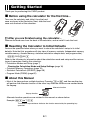
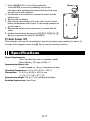
k Before using the calculator for the ﬁrst time...
Turn over the calculator and slide it from the hard
case as shown in the illustration. Next, slide the hard
case onto the back of the calculator.
A After you are ﬁnished using the calculator...
Remove the hard case from the back of the calculator, and re-install it onto the front.
k Resetting the Calculator to Initial Defaults
Perform the operation below when you want to return the calculator’s setup to its initial
defaults. Note that this procedure will also clear all memory contents (independent memory,
variable memory, Answer Memory, statistical calculation sample data, and program data).
!9(CLR)3(All)w
Refer to the following for information about the calculation mode and setup and the various
types of memories used by this calculator.
• Calculation Modes and Setup (page 7)
Clearing the Calculation Mode and Setup Settings (page 10)
• Calculator Memory Operations (page 19)
• Statistical Calculations (SD/REG) (page 38)
• Program Mode (PRGM) (page 62)
k About this Manual
• Most of the keys perform multiple functions. Pressing ! or a and then another key
will perform the alternate function of the other key. Alternate functions are marked above
the keycap.
Alternate function
sin–1{D}
Keycap function
s
Alternate function operations are notated in this manual as shown below.
–1
Example: !s(sin )bw
The notation in parentheses indicates the function executed by the preceding key
operation.
E-1
• The following shows the notation used in the manual for menu items that appear on the
display (which are executed by pressing a number key).
Example: b(Contrast)
The notation in parentheses indicates the menu item accessed by the preceding number
key.
• The cursor key is marked with arrows indicating direction as shown in the
illustration nearby. Cursor key operations are notated in this manual as:
f, c, d, and e.
REPLAY
• The displays and illustrations (such as key markings) shown in this User’s Guide are for
illustrative purposes only, and may differ somewhat from the actual items they represent.
• The contents of this manual are subject to change without notice.
• In no event shall CASIO Computer Co., Ltd. be liable to anyone for special, collateral,
incidental, or consequential damages in connection with or arising out of the purchase or
use of this product and items that come with it. Moreover, CASIO Computer Co., Ltd. shall
not be liable for any claim of any kind whatsoever by any other party arising out of the use
of this product and the items that come with it.
Safety Precautions
Be sure to read the following safety precautions before using this calculator. Keep this
manual handy for later reference.
Caution
This symbol is used to indicate information that can result in personal injury or material
damage if ignored.
Battery
• After removing the battery from the calculator, put it in a safe place where it will not
get into the hands of small children and accidentally swallowed.
• Keep batteries out of the reach of small children. If accidentally swallowed, consult
with a physician immediately.
• Never charge the battery, try to take the battery apart, or allow the battery to become
shorted. Never expose the battery to direct heat or dispose of it by incineration.
• Improperly using a battery can cause it to leak and damage nearby items, and can
create the risk of ﬁre and personal injury.
• Always make sure that the battery’s positive k and negative l ends are facing
correctly when you load it into the calculator.
• Use only the type of battery speciﬁed for this calculator in this manual.
Disposing of the Calculator
• Never dispose of the calculator by burning it. Doing so can cause certain components
to suddenly burst, creating the risk of ﬁre and personal injury.
E-2
Operating Precautions
• Be sure to press the O key before using the calculator for the ﬁrst time.
• Even if the calculator is operating normally, replace the battery at least once every
three years.
A dead battery can leak, causing damage to and malfunction of the calculator. Never
leave a dead battery in the calculator.
• The battery that comes with this unit discharges slightly during shipment and
storage. Because of this, it may require replacement sooner than the normal
expected battery life.
• Low battery power can cause memory contents to become corrupted or lost
completely. Always keep written records of all important data.
• Avoid use and storage of the calculator in areas subjected to temperature extremes.
Very low temperatures can cause slow display response, total failure of the display,
and shortening of battery life. Also avoid leaving the calculator in direct sunlight, near a
window, near a heater or anywhere else it might be exposed to very high temperatures.
Heat can cause discoloration or deformation of the calculator’s case, and damage to
internal circuitry.
• Avoid use and storage of the calculator in areas subjected to large amounts of
humidity and dust.
Take care never to leave the calculator where it might be splashed by water or exposed to
large amounts of humidity or dust. Such conditions can damage internal circuitry.
• Never drop the calculator or otherwise subject it to strong impact.
• Never twist or bend the calculator.
Avoid carrying the calculator in the pocket of your trousers or other tight-ﬁtting clothing
where it might be subjected to twisting or bending.
• Never try to take the calculator apart.
• Never press the keys of the calculator with a ballpoint pen or other pointed object.
• Use a soft, dry cloth to clean the exterior of the calculator.
If the calculator becomes very dirty, wipe it off with a cloth moistened in a weak solution
of water and a mild neutral household detergent. Wring out all excess liquid before wiping
the calculator. Never use thinner, benzene or other volatile agents to clean the calculator.
Doing so can remove printed markings and can damage the case.
E-3
Contents
Getting Started .........................................................................................1
Before using the calculator for the ﬁrst time... .................................................................... 1
Resetting the Calculator to Initial Defaults.......................................................................... 1
About this Manual............................................................................................................... 1
Safety Precautions ...................................................................................2
Operating Precautions .............................................................................3
Before starting a calculation... ................................................................6
Turning On the Calculator................................................................................................... 6
Key Markings ...................................................................................................................... 6
Reading the Display ........................................................................................................... 7
Calculation Modes and Setup .................................................................7
Selecting a Calculation Mode ............................................................................................. 7
Calculator Setup ................................................................................................................. 8
Clearing the Calculation Mode and Setup Settings .......................................................... 10
Inputting Calculation Expressions and Values ....................................10
Inputting a Calculation Expression (Natural Input) ........................................................... 10
Editing a Calculation......................................................................................................... 12
Finding the Location of an Error ....................................................................................... 13
Basic Calculations..................................................................................14
Arithmetic Calculations ..................................................................................................... 14
Fractions ........................................................................................................................... 14
Percent Calculations......................................................................................................... 16
Degree, Minute, Second (Sexagesimal) Calculations ...................................................... 17
Calculation History and Replay.............................................................18
Accessing Calculation History ......................................................................................... 18
Using Replay .................................................................................................................... 19
Calculator Memory Operations .............................................................19
Using Answer Memory (Ans) ........................................................................................... 19
Using Independent Memory ............................................................................................. 21
Using Variables ................................................................................................................. 22
Clearing All Memory Contents ......................................................................................... 23
Using π, e, and Scientiﬁc Constants .....................................................23
Pi (π) and Natural Logarithm Base e ................................................................................ 23
Scientiﬁc Constants .......................................................................................................... 24
Scientiﬁc Function Calculations ..........................................................26
Trigonometric and Inverse Trigonometric Functions ......................................................... 27
Angle Unit Conversion ...................................................................................................... 27
Hyperbolic and Inverse Hyperbolic Functions .................................................................. 28
Exponential and Logarithmic Functions ........................................................................... 28
Power Functions and Power Root Functions .................................................................... 29
E-4
Coordinate Conversion (Rectangular ↔ Polar) ................................................................ 29
Other Functions ................................................................................................................ 31
3
Using 10 Engineering Notation (ENG) .................................................33
ENG Calculation Examples .............................................................................................. 33
Complex Number Calculations (CMPLX) .............................................34
Inputting Complex Numbers ............................................................................................. 34
Complex Number Calculation Result Display ................................................................... 34
Calculation Result Display Examples ............................................................................... 35
Conjugate Complex Number (Conjg) ............................................................................... 36
Absolute Value and Argument (Abs, arg) ......................................................................... 36
Overriding the Default Complex Number Display Format................................................. 37
Statistical Calculations (SD/REG) ........................................................38
Statistical Calculation Sample Data ................................................................................. 38
Performing Single-variable Statistical Calculations .......................................................... 38
Performing Paired-variable Statistical Calculations .......................................................... 42
Statistical Calculation Examples ...................................................................................... 50
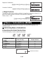
Base-n Calculations (BASE) ..................................................................52
Performing Base-n Calculations ....................................................................................... 52
Converting a Displayed Result to another Number Base ................................................. 54
Using the LOGIC Menu .................................................................................................... 54
Specifying a Number Base for a Particular Value ............................................................. 54
Performing Calculations Using Logical Operations and Negative Binary Values ............. 55
Built-in Formulas ....................................................................................56
Using Built-in Formulas .................................................................................................... 56
Built-in Formula List .......................................................................................................... 58
Program Mode (PRGM) ..........................................................................62
Program Mode Overview .................................................................................................. 62
Creating a Program .......................................................................................................... 63
Running a Program .......................................................................................................... 64
Deleting a Program........................................................................................................... 64
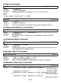
Inputting Commands ........................................................................................................ 65
Command Reference ....................................................................................................... 65
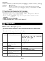
Appendix .................................................................................................71
Calculation Priority Sequence .......................................................................................... 71
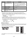
Stack Limitations .............................................................................................................. 72
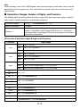
Calculation Ranges, Number of Digits, and Precision ...................................................... 73
Error Messages ................................................................................................................ 74
Before assuming malfunction of the calculator... ............................................................. 76
Power Requirements ..............................................................................76
Speciﬁcations .........................................................................................77
E-5
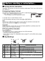
Before starting a calculation...
k Turning On the Calculator
Press O. The calculator will enter the calculation mode (page 7) that it was in the last time
you turned it off.
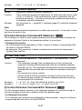
A Adjusting Display Contrast
If the ﬁgures on the display become hard to read, try adjusting display contrast.
1. Press !N(SETUP) db(Contrast).
L I GHT
• This will display the contrast adjustment screen.
DARK
CASIO
2. Use d and e to adjust display contrast.
3. After the setting is the way you want, press A or !p(EXIT).
Note
You can also use + and - to adjust contrast while the calculation mode menu that
appears when you press the , key is on the display.
Important!
If adjusting display contrast does not improve display readability, it probably means that
battery power is low. Replace the battery.
A Turning Off the Calculator
Press !A(OFF).
The following information is retained when you turn off the calculator.
• Calculation modes and setup (page 7)
• Answer Memory (page 19), independent memory (page 21), and variable memory (page
22) contents
k Key Markings
M–
x!
A
M
8
LOGIC
DT CL
Function
1
M+
Colors
To perform the function
Press the key.
2
M–
Text: Amber
Press ! and then press the key.
3
M
Text: Red
Press a and then press the key.
4
DT
Text: Blue
In the SD or REG Mode, press the key.
5
CL
Text: Amber
Frame: Blue
In the SD or REG Mode, press ! and then press
the key.
6
∠
Text: Amber
Frame: Purple
In the CMPLX Mode, press ! and then press the
key.
E-6
Function
7
A
8
LOGIC
Colors
To perform the function
Text: Red
Frame: Green
Press a and then press the key (variable A).
In the BASE Mode, press the key.
Text: Green
In the BASE Mode, press the key.
k Reading the Display
A Input Expressions and Calculation Results
This calculator can display both the expressions you input and calculation results on the
same screen.
2× ( 5+ 4 ) – 2× - 3
Input expression
24
Calculation result
A Display Symbols
The symbols described below appear on the display of the calculator to indicate the current
calculation mode, the calculator setup, the progress of calculations, and more. In this
manual, the expression “turn on” is used to mean that a symbol appears on the display, and
“turn off” means that it disappears.
The nearby sample screen shows the 7 symbol.
s i n ( 30 )
05
The 7 symbol turns on when degrees (Deg) are selected for the default angle unit (page
8). For information about the meaning of each symbol, see the section of this manual that
describes each function.
Calculation Modes and Setup
k Selecting a Calculation Mode
Your calculator has six “calculation modes”.
A Selecting a Calculation Mode
1. Press ,.
• This displays the calculation mode menu.
• The calculation mode menu has two screens. Press , to toggle between them. You
can also switch between menu screens using d and e.
COMP CMPLX BASE
SD
REG
1
4
5
2
3
E-7
PRGM
6
2. Perform one of the following operations to select the calculation mode you want.
To select this calculation mode:
Press this key:
COMP (Computation)
b(COMP)
CMPLX (Complex Number)
c(CMPLX)
BASE (Base n)
d(BASE)
SD (Single Variable Statistics)
e(SD)
REG (Paired Variable Statistics)
f(REG)
PRGM (Program)
g(PRGM)
• Pressing a number key from b to g selects the applicable mode, regardless of which
menu screen is currently displayed.
k Calculator Setup
The calculator setup can be used to conﬁgure input and output settings, calculation
parameters, and other settings. The setup can be conﬁgured using setup screens, which
you access by pressing !,(SETUP). There are six setup screens, and you can use
d and e to navigate between them.
A Specifying the Angle Unit
You can specify degrees, radians, or grads as the angle unit to be applied for trigonometric
function calculations.
π
(90˚ =
radians = 100 grads)
2
Angle Unit
Perform this key operation:
Degrees
!,b(Deg)
Radians
!,c(Rad)
Grads
!,d(Gra)
A Specifying the Display Digits
You can select any one of three settings for the calculation result display digits: ﬁxed
number of decimal places (0 to 9 places), ﬁxed number of signiﬁcant digits (1 to 10 digits),
or exponential display range (a choice of two settings).
Exponential Display
Perform this key operation:
Number of Decimal Places
!,eb(Fix)
a(0) to j(9)
Signiﬁcant Digits
!,ec(Sci)
b(1) to j(9), a(10)
Exponential Display Range
!,ed(Norm)
b(Norm1) or c(Norm2)
E-8
The following explains how calculation results are displayed in accordance with the setting
you specify.
• From zero to nine decimal places are displayed in accordance with the number of decimal
places (Fix) you specify. Calculation results are rounded off to the speciﬁed number of
digits.
Example: 100 ÷ 7 = 14.286 (Fix = 3)
14.29 (Fix = 2)
• After you specify the number of signiﬁcant digits with Sci, calculation results are
displayed using the speciﬁed number of signiﬁcant digits and 10 to the applicable power.
Calculation results are rounded off to the speciﬁed number of digits.
–1
(Sci = 5)
Example: 1 ÷ 7 = 1.4286 × 10
–1
(Sci = 4)
1.429 × 10
• Selecting Norm1 or Norm2 causes the display to switch to exponential notation whenever
the result is within the ranges deﬁned below.
–2
10
Norm1: 10 > x, x > 10
–9
10
Norm2: 10 > x, x > 10
Example: 100 ÷ 7 = 14.28571429 (Norm1 or Norm2)
–3
(Norm1)
1 ÷ 200 = 5. × 10
0.005
(Norm2)
A Specifying the Fraction Display Format
You can specify either improper fraction or mixed fraction format for display of calculation
results.
Fraction Format
Perform this key operation:
Mixed Fractions
!,eeb(ab/c)
Improper Fractions
!,eec(d/c)
A Specifying the Complex Number Display Format
You can specify either rectangular coordinate format or polar coordinate format for complex
number calculation results.
Complex Number Format
Perform this key operation:
Rectangular Coordinates
!,eeeb(a+bi)
Polar Coordinates
!,eeec(r∠Ƨ)
A Specifying the Statistical Frequency Setting
Use the key operations below to turn statistical frequency on or off during SD Mode and
REG Mode calculations.
Frequency Setting
Perform this key operation:
Frequency On
!,ddb(FreqOn)
Frequency Off
!,ddc(FreqOff)
E-9
k Clearing the Calculation Mode and Setup Settings
Perform the procedure described below to clear the current calculation mode and all setup
settings and initialize the calculator to the following.
Calculation Mode ................................ COMP (Computation Mode)
Angle Unit ........................................... Deg (Degrees)
Exponential Display ............................. Norm1
Fraction Format .................................. ab/c (Mixed Fractions)
Complex Number Format ................... a+bi (Rectangular Coordinates)
Frequency Setting .............................. FreqOn (Frequency On)
Perform the following key operation to clear the calculation mode and setup settings.
!9(CLR)2(Setup)w
If you do not want to clear the calculator’s settings, press A in place of w in the above
operation.
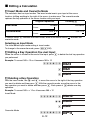
Inputting Calculation Expressions
and Values
k Inputting a Calculation Expression (Natural Input)
The natural input system of your calculator lets you input a calculation expression just as
it is written and execute it by pressing w. The calculator determines the proper priority
sequence for addition, subtraction, multiplication, division, functions and parentheses
automatically.
Example: 2 × (5 + 4) – 2 × (–3) =
2*(5+4)2*-3w
2× ( 5+ 4 ) – 2× - 3
24
A Inputting Scientiﬁc Functions with Parentheses (sin, cos, ',
etc.)
Your calculator supports input of the scientiﬁc functions with parentheses shown below.
Note that after you input the argument, you need to press ) to close the parentheses.
–1
–1
–1
–1
–1
–1
sin(, cos(, tan(, sin (, cos (, tan (, sinh(, cosh(, tanh(, sinh (, cosh (, tanh (, log(, ln(,
e^(, 10^(, '(, 3'(, Abs(, Pol(, Rec(, arg(, Conjg(, Not(, Neg(, Rnd(
Example: sin 30 =
s30)w
E-10
s i n ( 30 )
05
A Omitting the Multiplication Sign
You can omit the multiplication sign in the following cases.
• Immediately before an open parenthesis: 2 × (5 + 4)
• Immediately before a scientiﬁc function with parentheses: 2 × sin(30), 2 × '(3)
• Before a preﬁx symbol (excluding the minus sign): 2 × h123
• Before a variable name, constant, or random number: 20 × A, 2 × π, 2 × i
A Final Closed Parenthesis
You can omit one or more closed parentheses that come at the end of a calculation,
immediately before the w key is pressed.
Example: (2 + 3) × (4 – 1) = 15
(2+3)*
(4-1w
( 2+ 3 ) × ( 4– 1
15
• Simply press w without closing the parentheses. The above applies to the closing
parentheses at the end of the calculation only. Your calculation will not produce the correct
result if you forget the closing parentheses that are required before the end.
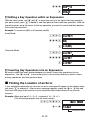
A Scrolling the Screen Left and Right
Inputting a mathematical expression that has more than 16 characters in it will cause the
screen to scroll automatically, causing part of the expression to move off of the display. The
“b” symbol on the left edge of the screen indicates that there is additional data off the left
side of the display.
Input Expression
12345 + 12345 + 12345
345 + 12345 + 12345I
Displayed Expression
Cursor
• While the b symbol is on the screen, you can use the d key to move the cursor to the
left and scroll the screen.
• Scrolling to the left causes part of the expression to run off the right side of the display,
which is indicated by the \ symbol on the right. While the \ symbol is on the screen,
you can use the e key to move the cursor to the right and scroll the screen.
• You can also press f to jump to the beginning of the expression, or c to jump to the
end.
A Number of Input Characters (Bytes)
As you input a mathematical expression, it is stored in memory called an “input area,”
which has a capacity of 99 bytes. This means you can input up to 99 bytes for a single
mathematical expression.
Normally, the cursor that indicates the current input location on the display is either a
ﬂashing vertical bar (|) or horizontal bar ( ). When the remaining capacity of the input area
is eight bytes or less, the cursor changes to a ﬂashing box (k).
If this happens, stop input of the current expression at some suitable location and calculate
its result.
E-11
k Editing a Calculation
A Insert Mode and Overwrite Mode
The calculator has two input modes. The insert mode inserts your input at the cursor
location, shifting anything to the right of the cursor to make room. The overwrite mode
replaces the key operation at the cursor location with your input.
Pressing +
Original Expression
Insert Mode
1+2|34
1+2+|34
1+2 3 4
1+2 + 4
Cursor
Overwrite Mode
Cursor
A vertical cursor (|) indicates the insert mode, while a horizontal cursor ( ) indicates the
overwrite mode.
Selecting an Input Mode
The initial default input mode setting is insert mode.
To change to the overwrite mode, press: 1D(INS).
A Editing a Key Operation You Just Input
When the cursor is located at the end of the input, press D to delete the last key operation
you performed.
Example: To correct 369 × 13 so it becomes 369 × 12
369*13
369 × 13I
D
369 × 1I
2
369 × 12I
A Deleting a Key Operation
With the insert mode, use d and e to move the cursor to the right of the key operation
you want to delete and then press D. With the overwrite mode, move the cursor to the
key operation you want to delete and then press D. Each press of D deletes one key
operation.
Example: To correct 369 × × 12 so it becomes 369 × 12
Insert Mode
369**12
369 ×× 12I
dd
369 ××I12
D
369 ×I12
Overwrite Mode
369**12
E-12
369 ×× 12
ddd
D
369 ×× 12
369 × 12
A Editing a Key Operation within an Expression
With the insert mode, use d and e to move the cursor to the right of the key operation
you want to edit, press D to delete it, and then perform the correct key operation. With the
overwrite mode, move the cursor to the key operation you want to correct and then perform
the correct key operation.
Example: To correct cos(60) so it becomes sin(60)
Insert Mode
c60)
cos ( 60 )I
dddD
I60 )
s
s i n ( I60 )
c60)
cos ( 60 )
dddd
cos ( 60 )
s
s i n ( 60 )
Overwrite Mode
A Inserting Key Operations into an Expression
Be sure to select the insert mode whenever you want to insert key operations into an
expression. Use d and e to move the cursor to the location where you want to insert
the key operations, and then perform them.
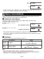
k Finding the Location of an Error
If your calculation expression is incorrect, an error message will appear on the display when
you press w to execute it. After an error message appears, press the d or e key and
the cursor will jump to the location in your calculation that caused the error so you can
correct it.
Example: When you input 14 ÷ 0 × 2 = instead of 14 ÷ 10 × 2 =
(The following examples use the insert mode.)
14/0*2w
e or d
Mat h ERROR
14 ÷ 0I×2
Location of Error
E-13
d1
w
14 ÷ 1I0×2
14 ÷ 10 × 2
28
• Instead of pressing e or d while an error message is displayed to ﬁnd the location of
the error, you could also press A to clear the calculation.
Basic Calculations
Unless otherwise noted, the calculations in this section can be performed in any of the
calculator’s calculation mode, except for the BASE Mode.
k Arithmetic Calculations
Arithmetic calculations can be used to perform addition (+), subtraction (-),
multiplication (*), and division (/).
Example 1: 2.5 + 1 − 2 = 1.5
2.5+1-2w
Example 2: 7 × 8 − 4 × 5 = 36
7*8-4*5w
2.5 + 1 – 2
15
7×8– 4×5
36
• The calculator determines the proper priority sequence for addition, subtraction,
multiplication, and division automatically. See “Calculation Priority Sequence” on page 71
for more information.
k Fractions
Fractions are input using a special separator symbol ({).
Key Operation
Improper
Fraction
7$3
Mixed
Fraction
2$1$3
Display
7{3
Numerator Denominator
2{1{3
Integer Numerator Denominator
Note
• Under initial default settings, fractions are displayed as mixed fractions.
• Fraction calculation results are always reduced automatically before being displayed.
Executing 2 { 4 = for example, will display the result 1 { 2.
E-14
A Fraction Calculation Examples
Example 1: 3
1
2
11
+1 =4
4
3
12
3$1$4+
1$2$3w
Example 2: 4 – 3
1
1
=
2
2
4-3$1$2w
2
1
7
Example 3:
+
=
(Fraction Display Format: d/c)
3
2
6
2$3+1$2w
3{1{4 + 1{2{3
4{11{12
4 – 3{1{2
2{3 + 1{2
1{2
7{6
Note
• If the total number of elements (integer + numerator + denominator + separator symbols)
of a fraction calculation result is greater than 10, the result will be displayed in decimal
format.
• If an input calculation includes a mixture of fraction and decimal values, the result will be
displayed in decimal format.
• You can input integers only for the elements of a fraction. Inputting non-integers will
produce a decimal format result.
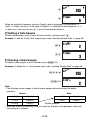
A Switching between Mixed Fraction and Improper Fraction
Format
To convert a mixed fraction to an improper fraction (or an improper fraction to a mixed
fraction), press !$(d/c).
A Switching between Decimal and Fraction Format
Use the procedure below to toggle a displayed calculation result between decimal and
fraction format.
1
1
Example: 1.5 = 1 , 1 = 1.5
2
2
1.5w
$
15
1{1{2
The current fraction display format setting determines if a
mixed or improper fraction is displayed.
$
15
Note
The calculator cannot switch from decimal to fraction format if the total number of fraction
elements (integer + numerator + denominator + separator symbols) is greater than 10.
E-15
k Percent Calculations
Inputting a value and with a percent (%) sign makes the value a percent. The percent (%)
sign uses the value immediately before it as the argument, which is simply divided by 100 to
get the percentage value.
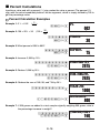
A Percent Calculation Examples
Example 1: 2 % = 0.02
(
2
)
10 0
Example 2: 150 × 20% = 30
2!((%)w
(150 ×
2%
002
20
)
10 0
150*20
!((%)w
150 × 20%
30
Example 3: What percent of 880 is 660?
660/880
!((%)w
660 ÷ 880%
75
Example 4: Increase 2,500 by 15%.
2500+2500*
15!((%)w
2500 + 2500 × 15%
2875
Example 5: Reduce 3,500 by 25%.
3500-3500*
25!((%)w
3500 – 3500 × 25%
2625
Example 6: Reduce the sum of 168, 98, and 734 by 20%.
168+98+734w
-G*20!((%)w
168 + 98 + 734
1000
Ans – Ans × 20%
800
Example 7: If 300 grams are added to a test sample originally weighing 500 grams, what is
the percentage increase in weight?
(500+300)
/500!((%)w
E-16
( 500 + 300 ) ÷ 500%
160
Example 8: What is the percentage change when a value is increased from 40 to 46? How
about to 48?
Insert Mode
(46-40)/40
!((%)w
eeeeY8w
( 46 – 40 ) ÷ 40%
15
( 48 – 40 ) ÷ 40%
20
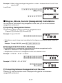
k Degree, Minute, Second (Sexagesimal) Calculations
You can perform calculations using sexagesimal values, and you can convert between
sexagesimal and decimal.
A Inputting Sexagesimal Values
The following is basic syntax for inputting a sexagesimal value.
{Degrees} $ {Minutes} $ {Seconds} $
Example: To input 2°30´30˝
2$30$30$w
2 ˚ 30 ˚ 30 ˚
2 ˚ 30 ˚ 30
• Note that you must always input something for the degrees and minutes, even if they are
zero.
Example: To input 0°00´30˝, press 0$0$30$.
A Sexagesimal Calculation Examples
The following types of sexagesimal calculations will produce sexagesimal results.
• Addition or subtraction of two sexagesimal values
• Multiplication or division of a sexagesimal value and a decimal value
Example 1: 2°20´30˝ + 39´30˝ = 3°00´00˝
2$20$30$+
0$39$30$w
2 ˚ 20 ˚ 30 ˚ + 0 ˚ 39 ˚ 30
3 ˚ 0˚ 0
Example 2: 2°20´00˝ × 3.5 = 8°10´00˝
2$20$*
3.5w
2 ˚ 20 ˚ × 3. 5
8 ˚ 10 ˚ 0
A Converting between Sexagesimal and Decimal
Pressing $ while a calculation result is displayed will toggle the value between
sexagesimal and decimal.
E-17
Example: To convert 2.255 to sexagesimal
2255
2 ˚ 15˚ 18
2255
2.255w
$
$
Calculation History and Replay
Calculation history maintains a record of each calculation you perform, including the
expressions you input and calculation results. You can use calculation history in the COMP,
CMPLX, and BASE Modes.
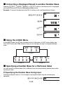
k Accessing Calculation History
The ` symbol in the upper right corner of the display indicates that there is data stored in
calculation history. To view the data in calculation history, press f. Each press of f will
scroll upwards (back) one calculation, displaying both the calculation expression and its
result.
Example:
1+1w2+2w
3+3w
f
f
3+ 3
6
2+2
4
1+1
2
While scrolling through calculation history records, the $ symbol will appear on the display,
which indicates that there are records below (newer than) the current one. When this
symbol is turned on, press c to scroll downwards (forward) through calculation history
records.
Important!
• Calculation history records are all cleared whenever you press p, when you change to a
different calculation mode, and whenever you perform any reset operation.
• Calculation history capacity is limited. Whenever you perform a new calculation while
calculation history is full, the oldest record in calculation history is deleted automatically to
make room for the new one.
E-18
k Using Replay
While a calculation history record is on the display, press d or e to display the cursor
and enter the editing mode. Pressing e displays the cursor at the beginning of the
calculation expression, while d displays it at the end. After you make the changes you
want, press w to execute the calculation.
Example: 4 × 3 + 2.5 = 14.5
4 × 3 – 7.1 = 4.9
4*3+2.5w
d
DDDD
-7.1w
4×3+ 2 . 5
145
4 × 3 + 2 . 5I
145
4 × 3I
145
4×3 –7 . 1
49
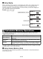
Calculator Memory Operations
Your calculator includes the types of memory described below, which you can use for
storage and recall of values.
Memory Name
Description
Answer Memory
Answer Memory contains the result of the last calculation you
performed.
Independent
Memory
Independent memory can be used in all calculation modes, except
for the SD Mode and the REG Mode.
Variables
Six variables named A, B, C, D, X, and Y can be used for temporary
storage of values. Variables can be used in all calculation modes.
The types of memory described above are not cleared when you press the A key, change
to another mode, or turn off the calculator.
k Using Answer Memory (Ans)
The result of any new calculation you perform on the calculator is stored automatically in
Answer Memory (Ans).
E-19
A Ans Update and Delete Timing
When using Ans in a calculation, it is important to keep in mind how and when its contents
change. Note the following points.
• The contents of Ans are replaced whenever you perform any of the following operations:
calculate a calculation result, add a value to or subtract a value from independent
memory, assign a value to a variable or recall the value of a variable, or input statistical
data in the SD Mode or REG Mode.
• In the case of a calculation that produces more than one result (like coordinate
calculations), the value that appears ﬁrst on the display is stored in Ans.
• The contents of Ans do not change if the current calculation produces an error.
• When you perform a complex number calculation in the CMPLX Mode, both the real part
and the imaginary part of the result are stored in Ans. Note, however, that the imaginary
part of the value is cleared if you change to another calculation mode.
A Automatic Insertion of Ans in Consecutive Calculations
If you start a new calculation while the result of a previous calculation is still on the display,
the calculator will insert Ans into the applicable location of the new calculation automatically.
Example 1: To divide the result of 3 × 4 by 30
3*4w
(Next) /30w
3×4
12
Ans ÷ 30
04
Pressing / inputs Ans automatically.
2
Example 2: To determine the square root of the result of 3 + 4
2
3x+4xw
9w
3 2 +4 2
25
'( Ans
5
Note
• As in the above examples, the calculator automatically inserts Ans as the argument of
any calculation operator or scientiﬁc function you input while a calculation result is on the
display.
• In the case of a function with parenthetical argument (page 10), Ans automatically
becomes the argument only in the case that you input the function alone and then press
w.
• Basically, Ans is inserted automatically only when the result of the previous calculation is
still on the display, immediately after you executed the calculation that produced it. See
the next section for information about inserting Ans into a calculation manually with the
K key.
E-20
A Inserting Ans into a Calculation Manually
You can insert Ans into a calculation at the current cursor location by pressing the K key.
Example 1: To use the result of 123 + 456 in another calculation as shown below
123 + 456 = 579
789 – 579 = 210
579
123+456w
789-Kw
2
789 – Ans
210
2
Example 2: To determine the square root of 3 + 4 , and then add 5 to the result
3x+4xw
9K)+5w
3 2 +4 2
25
'( Ans ) + 5
10
k Using Independent Memory
Independent memory (M) is used mainly for calculating cumulative totals.
If you can see the M symbol on the display, it means there is a non-zero value in
independent memory.
M symbol
10M+
10
A Adding to Independent Memory
While a value you input or the result of a calculation is on the display, press m to add it to
independent memory (M).
Example: To add the result of 105 ÷ 3 to independent memory (M)
105/3m
105 ÷ 3M+
35
A Subtracting from Independent Memory
While a value you input or the result of a calculation is on the display, press 1m(M–) to
subtract it from independent memory (M).
Example: To subtract the result of 3 × 2 from independent memory (M)
3*21m(M–)
E-21
3 × 2M–
6
Note
Pressing m or 1m(M–) while a calculation result is on the display will add it to or
subtract it from independent memory.
Important!
The value that appears on the display when you press m or 1m(M–) at the end of a
calculation in place of w is the result of the calculation (which is added to or subtracted
from independent memory). It is not the current contents of independent memory.
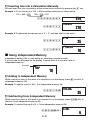
A Viewing Independent Memory Contents
Press tm(M).
A Clearing Independent Memory Contents (to 0)
01t(STO)m(M)
Clearing independent memory will cause the M symbol to turn off.
A Calculation Example Using Independent Memory
If the M symbol is displayed on your calculator screen, press 01t(STO)m(M) to
clear independent memory contents before performing the following operation.
Example:
23+9m
23 + 9 = 32
−)
53 – 6 = 47
53-6m
45 × 2 = 90
45*21m(M–)
99 ÷ 3 = 33
99/3m
(Total) 22
tm(M)
(Recalls value of M.)
k Using Variables
The calculator supports six variables named A, B, C, D, X, and Y, which you can use to store
values as required.
A Assigning a Value or Calculation Result to a Variable
Use the procedure shown below to assign a value or a calculation expression to a variable.
Example: To assign 3 + 5 to variable A
3+51t(STO)-(A)
A Viewing the Value Assigned to a Variable
To view the value assigned to a variable, press t and then specify the variable name.
Example: To view the value assigned to variable A
t-(A)
A Using a Variable in a Calculation
You can use variables in calculations the same way you use values.
Example: To calculate 5 + A
5+a-(A)w
E-22
A Clearing the Value Assigned to a Variable (to 0)
Example: To clear variable A
01t(STO)-(A)
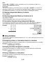
A Calculation Example Using Variables
Example: To perform calculations that assign results to variables B and C, and then use the
variables to perform another calculation
9×6+3
5 × 8 = 1.425
9*6+3
1t(STO)$(B)
5*8
1t(STO)w(C)
S$(B)/
Sw(C)w
9 × 6 + 3→B
5 × 8→C
57
40
B÷ C
1425
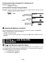
k Clearing All Memory Contents
Perform the following key operation when you want to clear the contents of independent
memory, variable memory, and Answer Memory.
19(CLR)1(Mem)w
• If you do not want to clear the calculator’s settings, press A in place of w in the above
operation.
Using π, e, and Scientiﬁc
Constants
k Pi (π) and Natural Logarithm Base e
The calculator supports input of pi (π) and natural logarithm base e into calculations. π and
e are supported in all modes, except for the BASE Mode. The following are the values that
the calculator applies for each of the built-in constants.
π = 3.14159265358980 (1e(π))
e = 2.71828182845904 (Si(e))
E-23
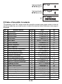
k Scientiﬁc Constants
Your calculator has 40 often-used scientiﬁc constants built in. Like π and e, each scientiﬁc
constant has a unique display symbol. Scientiﬁc constants are supported in all modes,
except for the BASE Mode.
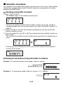
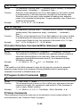
A Inputting a Scientiﬁc Constant
1. Press 17(CONST).
• This displays page 1 of the scientiﬁc constant menu.
mp mn ne m μ
1 2 3 4
• There are 10 scientiﬁc command menu screens, and you can use e and d to
navigate between them. For more information, see “Table of Scientiﬁc Constants” on
page 25.
2. Use e and d to scroll through the pages and display the one that contains the
scientiﬁc constant you want.
3. Press the number key (from 1 to 4) that corresponds to the scientiﬁc constant you
want to select.
• This will input the scientiﬁc constant symbol that corresponds to the number key you
press.
mp mn ne m μ
1 2 3 4
\
m pI
0
• Pressing E here will display the value of the scientiﬁc constant whose symbol is
currently on the screen.
mp
167262171 –27
A Example Calculations Using Scientiﬁc Constants
Example 1: To input the constant for the speed of light in a vacuum
17(CONST)
dddd4(c0)E
Example 2: To calculate the speed of light in a vacuum ( c0
299792458
= 1/ ε 0µ 0 )
1/9
E-24
C0
1 ÷'(I
0
17(CONST)
ddd4(ε0)
1 ÷'( ε0I
17(CONST)
dd1(ƫ0))
1 ÷'( ε 0 μ0 )I
E
0
0
1 ÷'( ε 0 μ0 )
299792458
A Table of Scientiﬁc Constants
The numbers in the “No.” column show the scientiﬁc constant menu page number on the left
and the number key you need to press to select the constant when the proper menu page is
displayed.
No.
Scientiﬁc Constant
Symbol
Value
Unit
–27
kg
–27
kg
–31
kg
–28
kg
1-1
Proton mass
mp
1.67262171×10
1-2
Neutron mass
mn
1.67492728×10
1-3
Electron mass
me
9.1093826×10
1-4
Muon mass
mƫ
1.8835314×10
2-1
Bohr radius
a0
0.5291772108×10
2-2
Planck constant
h
6.6260693×10
2-3
Nuclear magneton
µN
5.05078343×10
2-4
Bohr magneton
µB
927.400949×10
–10
m
–34
Js
–27
JT
–1
–26
JT
–1
–34
3-1
Planck constant, rationalized
3-2
Fine-structure constant
α
1.05457168×10
3-3
Classical electron radius
re
2.817940325×10
3-4
Compton wavelength
λc
2.426310238×10
4-1
Proton gyromagnetic ratio
γp
−
–15
m
–12
8
2.67522205×10
–15
4-2
Proton Compton wavelength
λcp
1.3214098555×10
4-3
Neutron Compton wavelength
λcn
1.3195909067×10
4-4
Rydberg constant
R∞
–15
10973731.568525
–27
5-1
Atomic mass constant
u
1.66053886×10
5-2
Proton magnetic moment
µp
1.41060671×10
m
–1
s T
–1
m
m
m
–1
kg
–26
JT
–1
–26
JT
–1
–26
JT
–1
–26
JT
–1
5-3
Electron magnetic moment
µe
–928.476412×10
5-4
Neutron magnetic moment
µn
–0.96623645×10
6-1
Muon magnetic moment
µƫ
–4.49044799×10
6-2
Faraday constant
F
6-3
Elementary charge
e
E-25
Js
–3
7.297352568×10
96485.3383
–19
1.60217653×10
C mol
C
–1
No.
Scientiﬁc Constant
Symbol
6-4
Avogadro constant
NA
7-1
Boltzmann constant
k
7-2
Molar volume of ideal gas
Vm
7-3
Molar gas constant
R
Value
Unit
23
mol
–23
JK
–3
m mol
6.0221415×10
1.3806505×10
8.314472 J mol
Speed of light in vacuum
C0
8-1
First radiation constant
C1
8-2
Second radiation constant
C2
8-3
Stefan-Boltzmann constant
σ
8-4
Electric constant
ε0
8.854187817×10
9-1
Magnetic constant
µ0
12.566370614×10
9-2
Magnetic ﬂux quantum
φ0
9-3
Standard acceleration of gravity
g
9-4
Conductance quantum
G0
10-1
Characteristic impedance of
vacuum
Z0
10-2 Celsius temperature
t
10-3 Newtonian constant of gravitation
G
10-4 Standard atmosphere
3
22.413996×10
7-4
299792458
ms
–1
K
–2
mK
2
–8
Wm K
–12
Fm
–7
NA
5.670400×10
–2
–4
–1
–2
–15
2.06783372×10
Wb
9.80665
ms
–5
S
7.748091733×10
–2
Ω
376.730313461
273.15
–11
–1
–1
Wm
1.4387752×10
atm
–1
–16
3.74177138×10
6.6742×10
–1
–1
K
3
–1
–2
m kg s
101325
Pa
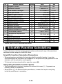
• Source: 2000 CODATA recommended values
Scientiﬁc Function Calculations
Unless otherwise noted, the functions in this section can be used in any of the calculator’s
calculation modes, except for the BASE Mode.
Scientiﬁc Function Calculation Precautions
• When performing a calculation that includes a built-in scientiﬁc function, it may take
some time before the calculation result appears. Do not perform any key operation on the
calculator until the calculation result appears.
• To interrupt and on-going calculation operation, press A.
Interpreting Scientiﬁc Function Syntax
• Text that represents a function’s argument is enclosed in braces ({ }). Arguments are
normally {value} or {expression}.
• When braces ({ }) are enclosed within parentheses, it means that input of everything
inside the parentheses is mandatory.
E-26
k Trigonometric and Inverse Trigonometric Functions
–1
–1
–1
sin(, cos(, tan(, sin (, cos (, tan (
A Syntax and Input
–1
–1
–1
sin({n}), cos({n}), tan({n}), sin ({n}), cos ({n}), tan ({n})
–1
Example: sin 30 = 0.5, sin 0.5 = 30 (Angle Unit: Deg)
s30)w
–1
1s(sin )0.5)w
s i n ( 30 )
05
s i n –1 ( 0. 5 )
30
A Notes
• These functions can be used in the CMPLX Mode, as long as a complex number is not
used in the argument. A calculation like i × sin(30) is supported for example, but sin(1 + i)
is not.
• The angle unit you need to use in a calculation is the one that is currently selected as the
default angle unit.
k Angle Unit Conversion
You can convert a value that was input using one angle unit to another angle unit.
After you input a value, press 1G(DRG') to display the menu screen shown below.
D
R
G
1 2 3
Example: To convert
1(D): Degrees
2(R): Radians
3(G): Grads
π
radians and 50 grads both to degrees
2
The following procedure assumes that Deg (degrees) is currently speciﬁed for the default
angle unit.
(1e(π)/2)
1G(DRG')2(R)E
501G(DRG')
3(G)E
E-27
( π ÷2 ) r
90
50 g
45
k Hyperbolic and Inverse Hyperbolic Functions
–1
–1
–1
sinh(, cosh(, tanh(, sinh (, cosh (, tanh (
A Syntax and Input
–1
–1
–1
sinh({n}), cosh({n}), tanh({n}), sinh ({n}), cosh ({n}), tanh ({n})
Example: sinh 1 = 1.175201194
ws(sinh)1)E
s i nh ( 1 )
1175201194
A Notes
• After pressing w to specify a hyperbolic function or 1w to specify an inverse
hyperbolic function, press s, c, or t.
• These functions can be used in the CMPLX Mode, but complex number arguments are
not supported.
k Exponential and Logarithmic Functions
10^(, e^(, log(, ln(,
A Syntax and Input
10^({n}) .......................... 10 n
log({n}) ........................... log10{n}
log({m},{n}) ..................... log{m}{n}
ln({n}) ............................. loge{n}
{ }
(Same applies to e^(.)
(Common Logarithm)
(Base {m} Logarithm)
(Natural Logarithm)
Example 1: log216 = 4, log16 = 1.204119983
l2,16)E
l16)E
l o g ( 2, 16 )
4
l o g ( 16 )
1204119983
Base 10 (common logarithm) is assumed when no base is speciﬁed.
Example 2: ln 90 (loge 90) = 4.49980967
I90)E
I n ( 90 )
449980967
10
Example 3: e = 22026.46579
x
1I(e )10)E
E-28
e ˆ ( 10 )
2202646579
k Power Functions and Power Root Functions
x2, x3, x–1, ^(, '(, 3'(, x'(
A Syntax and Input
2
2
{n} x ............................... {n}
3
3
{n} x ............................... {n}
–1
–1
{n} x ............................. {n}
{ }
{(m)}^({n}) ....................... {m} n
'({n}) .......................... {n}
3
3
'({n}) ......................... {n}
{ }
({m})x'({n}) .................. m {n}
(Square)
(Cube)
(Reciprocal)
(Power)
(Square Root)
(Cube Root)
(Power Root)
Example 1: ('
2 + 1) ('
2 – 1) = 1, (1 + 1)
2+2
= 16
(92)+1)
(92)-1)E
(1+1)M2+2)E
('( 2 ) + 1 ) ('( 2 ) – 1 )
1
( 1+ 1 ) ˆ ( 2+2 )
2
Example 2: –2 3 = –1.587401052
-2M2$3)E
16
– 2ˆ ( 2{3 )
-1587401052
A Notes
2
3
–1
• The functions x , x , and x can be used in complex number calculations in the CMPLX
Mode. Complex number arguments are also supported for these functions.
3
• ^(, '(, '(, x'( are also supported in the CMPLX Mode, but complex number
arguments are not supported for these functions.
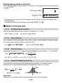
k Coordinate Conversion (Rectangular ↔ Polar)
Pol(, Rec(
Your calculator can convert between rectangular coordinates and polar coordinates.
o
o
Rectangular Coordinates (Rec)
E-29
Polar Coordinates (Pol)
A Syntax and Input
Rectangular-to-Polar Coordinate Conversion (Pol)
Pol(x, y)
x: Rectangular coordinate x-value
y: Rectangular coordinate y-value
Polar-to-Rectangular Coordinate Conversion (Rec)
Rec(r, Ƨ)
r: Polar coordinate r-value
Ƨ: Polar coordinate Ƨ-value
Example 1: To convert the rectangular coordinates ('
2, '
2 ) to polar coordinates
(Angle Unit: Deg)
1+(Pol)92)
,92))E
t,(Y)
(View the value of Ƨ)
Po l ('( 2 ) ,'( 2 ) )
2
Y
45
Example 2: To convert the polar coordinates (2, 30°) to rectangular coordinates
(Angle Unit: Deg)
1-(Rec)2,
30)E
t,(Y)
(View the value of y)
Rec ( 2, 30 )
1732050808
Y
1
A Notes
• These functions can be used in the COMP, SD, and REG Modes.
• Calculation results show the ﬁrst r value or x value only.
• The r-value (or x-value) produced by the calculation is assigned to variable X, while the
Ƨ-value (or y-value) is assigned to variable Y (page 22). To view the Ƨ-value (or y-value),
display the value assigned to variable Y, as shown in the example.
• The values obtained for Ƨ when converting from rectangular coordinates to polar
coordinates is within the range –180°< Ƨ < 180°.
• When executing a coordinate conversion function inside of a calculation expression, the
calculation is performed using the ﬁrst value produced by the conversion (r-value or xvalue).
2, '
2)+5=2+5=7
Example: Pol ('
E-30
k Other Functions
x!, Abs(, Ran#, nPr, nCr, Rnd(
The x!, nPr, and nCr functions can be used in the CMPLX Mode, but complex number
arguments are not supported.
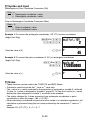
A Factorial (!)
Syntax: {n}! ({n} must be a natural number or 0.)
Example: (5 + 3)!
(5+3)
1X(x!)E
(5+3 ) !
40320
A Absolute Value (Abs)
When you are performing a real number calculation, Abs( simply obtains the absolute value.
This function can be used in the CMPLX Mode to determine the absolute value (size) of a
complex number. See “Complex Number Calculations” on page 34 for more information.
Syntax: Abs({n})
Example: Abs (2 – 7) = 5
1)(Abs)2-7)E
Abs ( 2 – 7 )
5
A Random Number (Ran#)
This function generates a three-decimal place (0.000 to 0.999) pseudo random number. It
does not require an argument, and can be used the same way as a variable.
Syntax: Ran#
Example: To use 1000Ran# to obtain three 3-digit random numbers.
10001.(Ran#)E
E
E
1000Ran#
287
1000Ran#
613
1000Ran#
118
• The above values are provided for example only. The actual values produced by your
calculator for this function will be different.
E-31
A Permutation (nPr)/Combination (nCr)
Syntax: {n}P{m}, {n}C{m}
Example: How many four-person permutations and combinations are possible for a group
of 10 people?
101*(nPr)4E
101/(nCr)4E
10P4
5040
10C4
210
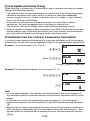
A Rounding Function (Rnd)
You can use the rounding function (Rnd) to round the value, expression, or calculation result
speciﬁed by the argument. Rounding is performed to the number of signiﬁcant digits in
accordance with the number of display digits setting.
Rounding for Norm1 or Norm2
The mantissa is rounded off to 10 digits.
Rounding for Fix or Sci
The value is rounded to the speciﬁed number of digits.
Example: 200 ÷ 7 × 14 = 400
200/7*14E
200 ÷ 7 × 14
400
(3 decimal places)
1Ne1(Fix)3
(Internal calculation uses 15 digits.)
200/7E
*14E
200 ÷ 7 × 14
400000
200 ÷ 7
28571
Ans × 14
400000
Now perform the same calculation using the rounding (Rnd) function.
200/7E
(Calculation uses rounded value.)
10(Rnd)E
E-32
200 ÷ 7
28571
Rnd ( Ans
28571
*14E
(Rounded result)
Ans × 14
399994
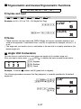
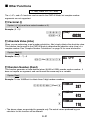
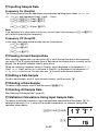
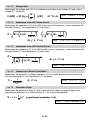
Using 103 Engineering Notation
(ENG)
Engineering notation (ENG) expresses quantities as a product of a positive number
between 1 and 10 and a power of 10 that is always a multiple of three. There are two types
of engineering notation, ENG/ and ENG,.
Function
Key Operation
ENG/
W
ENG,
1W(,)
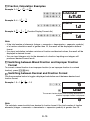
k ENG Calculation Examples
Example 1: To convert 1234 to engineering notation using ENG/
1234E
W
W
1234
1234
1234
1234
1234 03
1234 00
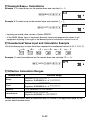
Example 2: To convert 123 to engineering notation using ENG,
123E
1W(,)
1W(,)
E-33
123
123
123
123
0123 03
0000123 06
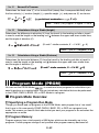
Complex Number Calculations
(CMPLX)
To perform the example operations in this section, ﬁrst select CMPLX (N2) as the
calculation mode.
k Inputting Complex Numbers
A Inputting Imaginary Numbers (i)
In the CMPLX Mode, the W key is used to input the imaginary number i. Use W(i) when
inputting complex numbers using rectangular coordinate format (a+bi).
Example: To input 2 + 3i
2+3W(i)
2 + 3 iI
A Inputting Complex Number Values Using Polar Coordinate
Format
Complex numbers can also be input using polar coordinate format (r ∠ Ƨ).
Example: To input 5 ∠ 30
51-(∠)30
5 30I
Important!
When inputting argument Ƨ, enter a value that indicates an angle in accordance with the
calculator’s current default angle unit setting.
k Complex Number Calculation Result Display
When a calculation produces a complex number result, R⇔I symbol turns on in the upper
right corner of the display and the only the real part appears at ﬁrst. To toggle the display
between the real part and the imaginary part, press 1E(Re⇔Im).
Example: To input 2 + 1i and display its calculation result
Before starting the calculation, you need to perform the following operation to change the
complex number display setting to “a+bi” as shown below.
To select rectangular coordinate format: 1,(SETUP)eee1(a+bi)
2+W(i)E
2+ i
2
Displays real part.
E-34
1E(Re⇔Im)
2+ i
1
Displays imaginary part.
(i symbol turns on during imaginary part display.)
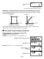
A Default Complex Number Calculation Result Display Format
You can select either rectangular coordinate format or polar coordinate format for complex
number calculation results.
Imaginary axis
Imaginary axis
o
r /u
a + bi
b
a
Real axis
Real axis
o
Rectangular Coordinates
Polar Coordinates
Use the setup screens to specify the default display format you want. For details, see
“Specifying the Complex Number Display Format” (page 9).
k Calculation Result Display Examples
A Rectangular Coordinate Format (a+bi)
1,(SETUP)eee1(a+bi)
Example 1: 2 × ('
3 + i) = 2'
3 + 2i = 3.464101615 + 2i
2*(93)+W(i))E
2 × ('( 3 ) + i )
1E(Re⇔Im)
2 × ('( 3 ) + i )
3464101615
Example 2: '
2 ∠ 45 = 1 + 1i (Angle Unit: Deg)
92)1-(∠)
45E
1E(Re⇔Im)
E-35
'( 2 ) 45
'( 2 ) 45
2
1
1
A Polar Coordinate Format (r∠Ƨ)
1,(SETUP)eee2(r∠Ƨ)
Example 1: 2 × ('
3 + i) = 2'
3 + 2i = 4 ∠ 30
2*(93)+W(i))E
2 × ('( 3 ) + i )
1E(Re⇔Im)
2 × ('( 3 ) + i )
4
30
∠ symbol turns on during display of Ƨ-value.
Example 2: 1 + 1i = 1.414213562 ∠ 45 (Angle Unit: Deg)
1+1W(i)E
1E(Re⇔Im)
1 +1 i
1414213562
1 +1 i
45
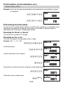
k Conjugate Complex Number (Conjg)
You can perform the operation below to obtain conjugate complex number ¯z = a + bi for the
complex number z = a + bi.
Example: Obtain the conjugate complex number of 2 + 3i
1,(Conjg)2+3W(i))E
1E(Re⇔Im)
Con jg( 2 + 3 i )
Con jg( 2 + 3 i )
2
-3
k Absolute Value and Argument (Abs, arg)
You can use the procedure shown below to obtain the absolute value (|z|) and argument (arg)
on the Gaussian plane for a complex number in the format z = a + bi.
Example:
Imaginary axis
To obtain the absolute value and argument of 2 + 2i
b=2
(Angle Unit: Deg)
o
E-36
a=2
Real axis
Absolute Value:
1)(Abs)2+2W(i))E
Abs ( 2 + 2 i )
2828427125
Argument:
1((arg)2+2W(i))E
ar g( 2 + 2 i )
45
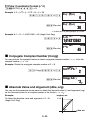
k Overriding the Default Complex Number Display Format
You can use the procedures described below to override the default complex number
display format and specify a particular display format for the calculation you are currently
inputting.
A Specifying Rectangular Coordinate Format for a Calculation
Input 1-('a+bi) at the end of the calculation.
2 ∠ 45 = 2 + 2i (Angle Unit: Deg)
Example: 2'
292)1-(∠)45
1-('a+bi)E
1E(Re⇔Im)
2' ( 2 ) 45 a + b i
2
2' ( 2 ) 45 a + b i
2
A Specifying Polar Coordinate Format for a Calculation
Input 1+('r∠Ƨ) at the end of the calculation.
Example: 2 + 2i = 2'
2 ∠ 45 = 2.828427125 ∠ 45 (Angle Unit: Deg)
2+2W(i)
1+('r∠Ƨ)E
1E(Re⇔Im)
E-37
2+2 i r θ
2828427125
2+2 i r θ
45
Statistical Calculations (SD/REG)
k Statistical Calculation Sample Data
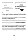
A Inputting Sample Data
You can input sample data either with statistical frequency turned on (FreqOn) or off (FreqOff).
The calculator’s initial default setting is FreqOn. You can select the input method you want
to use with the setup screen statistical frequency setting (page 9).
A Maximum Number of Input Data Items
The maximum number of data items you can input depends on whether frequency is on
(FreqOn) or off (FreqOff).
Frequency Setting
FreqOn
FreqOff
SD Mode
40 items
80 items
REG Mode
26 items
40 items
Calculation Mode
A Sample Data Clear
All sample data currently in memory is cleared whenever you change to another calculation
mode and when you change the statistical frequency setting.
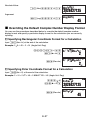
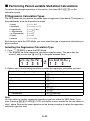
k Performing Single-variable Statistical Calculations
To perform the example operations in this section, ﬁrst select SD (N4) as the calculation
mode.
A Inputting Sample Data
Frequency On (FreqOn)
The following shows the key operations required when inputting class values x1, x2, ...xn,
and frequencies Freq1, Freq2, ... Freqn.
{x1}1,(;) {Freq1}m(DT)
{x2}1,(;) {Freq2}m(DT)
{xn}1,(;) {Freqn}m(DT)
Note
If the frequency of a class value is only one, you can input it by pressing {xn}m(DT) only
(without specifying the frequency).
E-38
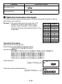
Example: To input the following data
Class Value (x)
Frequency (Freq)
24.5
4
25.5
6
26.5
2
24.51,(;)4
m(DT)
24 .5 ; 4I
0
L i ne =
1
m(DT) tells the calculator this is the end of the ﬁrst data item.
25.51,(;)6m(DT)
26.51,(;)2m(DT)
L i ne =
2
L i ne =
3
Frequency Off (FreqOff)
In this case, input each individual data item as shown below.
{x1}m(DT) {x2}m(DT) ... {xn}m(DT)
A Viewing Current Sample Data
After inputting sample data, you can press c to scroll through the data in the sequence
you input it. The $ symbol indicates there is data below the sample that is currently on the
display. The ` symbol indicates there is data above.
Example: To view the data you input in the example under “Inputting Sample Data” on page
38 (Frequency Setting: FreqOn)
A
c
c
E-39
I
0
x 1=
245
F r e q 1=
4
c
c
x 2=
255
F r eq2=
6
When the statistical frequency setting is FreqOn, data is displayed in the sequence: x1,
Freq1, x2, Freq2, and so on. In the case of FreqOff, it is displayed in the sequence: x1, x2,
x3, and so on. You can also use f to scroll in the reverse direction.
A Editing a Data Sample
To edit a data sample, recall it, input the new value(s), and then press E.
Example: To edit the “Freq3” data sample input under “Inputting Sample Data” on page 38
Af
3E
F r eq3=
2
F r eq3=
3
A Deleting a Data Sample
To delete a data sample, recall it and then press 1m(CL).
Example: To delete the “x2” data sample input under “Inputting Sample Data” on page 38
Accc
1m(CL)
x 2=
255
L i ne =
2
Note
• The following shows images of how the data appears before and after the delete
operation.
Before
After
x1: 24.5
Freq1: 4
x1: 24.5
Freq1: 4
x2: 25.5
Freq2: 6
x2: 26.5
Freq2: 2
x3: 26.5
Freq3: 2
Shifted upwards.
• When the statistical frequency setting is turned on (FreqOn), the applicable x-data and
Freq data pair is deleted.
E-40
A Deleting All Sample Data
Perform the following key operation to delete all sample data.
19(CLR)1(Stat)E
If you do not want to delete all sample data, press A in place of E in the above operation.
A Statistical Calculations Using Input Sample Data
To perform a statistical calculation, input the applicable command and then press E. To
determine the mean (o) value of the current input sample data, for example, perform the
operation shown below.
x xσn xσn–1
12(S-VAR)
1 2
3
x
1E
2533333333
* This is one example of possible calculation results.
A SD Mode Statistical Command Reference
xσn
11(S-SUM)1
ƙx2
Obtains the sum of squares of the sample
data.
xσn =
Σx2 = Σxi
2
11(S-SUM)2
ƙx
Obtains the sum of the sample data.
xσn–1
11(S-SUM)3
12(S-VAR)1
x¯
minX
Σ(xi – o)2
n–1
12(S-VAR)e1
Determines the minimum value of the
samples.
Obtains the mean.
Σx
o= ni
12(S-VAR)3
xσn –1 =
Obtains the number of samples.
n = (number of x-data items)
Σ(xi – o)2
n
Obtains the sample standard deviation.
Σx = Σxi
n
12(S-VAR)2
Obtains the population standard deviation.
maxX
12(S-VAR)e2
Determines the maximum value of the
samples.
E-41
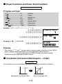
k Performing Paired-variable Statistical Calculations
To perform the example operations in this section, ﬁrst select REG (N5) as the
calculation mode.
A Regression Calculation Types
The REG Mode lets you perform the seven types of regression listed below. The ﬁgures in
the parentheses show the theoretical formulas.
• Linear
• Quadratic
• Logarithmic
• e Exponential
• ab Exponential
• Power
• Inverse
(y = a + bx)
2
(y = a+ bx + cx )
(y = a + b lnx)
(y = aebx)
(y = abx)
(y = axb)
(y = a + b/x)
Each time you enter the REG Mode, you must select the type of regression calculation you
plan to perform.
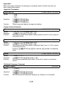
Selecting the Regression Calculation Type
1. Press N5(REG) to enter the REG Mode.
• This displays the initial regression calculation selection menu. The menu has two
screens, and you can use d and e to navigate between them.
L i n Lo g E x p Pwr
I nv Quad AB – Ex p
1 2 3 4
1 2
3
2. Perform one of the following operations to select the regression calculation you want.
To select this regression type:
And press this key:
Linear
1(Lin)
Logarithmic
2(Log)
e Exponential
3(Exp)
Power
4(Pwr)
Inverse
e1(Inv)
Quadratic
e2(Quad)
ab Exponential
e3(AB-Exp)
Note
You can switch to another regression calculation type from within the REG Mode, if you
want. Pressing 12(S-VAR)3(TYPE) will display a menu screen like the one shown in
step 1 above. Perform the same operation as the above procedure to select the regression
calculation type you want.
E-42
A Inputting Sample Data
Frequency On (FreqOn)
The following shows the key operations required when inputting class values (x1, y1), (x2,
y2), ...(xn, yn), and frequencies Freq1, Freq2, ... Freqn.
{x1},{y1}1,(;) {Freq1} m(DT)
{x2},{y2}1,(;) {Freq2} m(DT)
{xn},{yn}1,(;) {Freqn} m(DT)
Note
If the frequency of a class value is only one, you can input it by pressing {xn},{yn}m(DT)
only (without specifying the frequency).
Frequency Off (FreqOff)
In this case, input each individual data item as shown below.
{x1},{y1} m(DT)
{x2},{y2} m(DT)
{xn},{yn} m(DT)
A Viewing Current Sample Data
After inputting sample data, you can press c to scroll through the data in the sequence
you input it. The $ symbol indicates there is data below the sample that is currently on the
display. The ` symbol indicates there is data above.
When the statistical frequency setting is FreqOn, data is displayed in the sequence: x1, y1,
Freq1, x2, y2, Freq2, and so on. In the case of FreqOff, it is displayed in the sequence: x1,
y1, x2, y2, x3, y3, and so on. You can also use f to scroll in the reverse direction.
A Editing a Data Sample
To edit a data sample, recall it, input the new value(s), and then press E.
A Deleting a Data Sample
To delete a data sample, recall it and then press 1m(CL).
A Deleting All Sample Data
See “Deleting All Sample Data” (page 41).
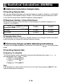
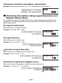
A Statistical Calculations Using Input Sample Data
To perform a statistical calculation, input the applicable command and then press E. To
determine the mean (o or p) value of the current sample data, for example, perform the
operation shown below.
x xσn xσn–1
12(S-VAR)1(VAR)
1E
E-43
1 2
3
x
115
y
12(S-VAR)1(VAR)e
yσn
1 2
yσn–1
3
y
1E
14
* This is one example of possible calculation results.
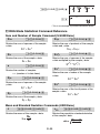
A REG Mode Statistical Command Reference
Sum and Number of Sample Command (S-SUM Menu)
ƙx2
11(S-SUM)1
Obtains the sum of squares of the sample
x-data.
ƙxy
Σx2 = Σxi2
ƙx
Σx = Σxi
n
Σxy = Σxiyi
11(S-SUM)2
Obtains the sum of the sample x-data.
ƙx2y
Σx2y = Σxi2yi
ƙx3
Obtains the number of samples.
ƙy2
ƙy
Σx3 = Σxi3
11(S-SUM)e1
11(S-SUM)e2
11(S-SUM)d2
Obtains the sum of cubes of the sample
x-data.
Obtains the sum of squares of the sample
y-data.
Σy2 = Σyi2
11(S-SUM)d1
Obtains the sum of squares of the sample
x-data multiplied by the sample y-data.
11(S-SUM)3
n = (number of x-data items)
11(S-SUM)e3
Obtains the sum of products of the sample
x-data and y-data.
ƙx4
11(S-SUM)d3
Obtains the sum of the fourth power of the
sample x-data.
Σx4 = Σxi4
Obtains the sum of the sample y-data.
Σy = Σyi
Mean and Standard Deviation Commands (VAR Menu)
x¯
xσn
12(S-VAR)1(VAR)1
Obtains the mean of the sample x-data.
Σx
o= ni
12(S-VAR)1(VAR)2
Obtains the population standard deviation
of the sample x-data.
xσn =
E-44
Σ(xi – o)2
n
xσn–1
yσn
12(S-VAR)1(VAR)3
Obtains the sample standard deviation of
the sample x-data.
xσn –1 =
12(S-VAR)1(VAR)e2
Obtains the population standard deviation
of the sample y-data.
Σ(xi – o)2
n–1
yσn =
Σ (yi – y)2
n
yσn–1 12(S-VAR)1(VAR)e3
y¯
Obtains the sample standard deviation of
the sample y-data.
12(S-VAR)1(VAR)e1
Obtains the mean of the sample y-data.
Σy
p = ni
yσn –1 =
Σ (yi – y)2
n–1
Regression Coefﬁcient and Estimated Value Commands for Nonquadratic Regression (VAR Menu)
The calculation that is performed when one of these commands is performed depends on
the regression type that is currently selected. For details about each regression calculation
formula, see “Regression Coefﬁcient and Estimated Value Calculation Formula Table” (page
47).
12(S-VAR)1(VAR)ee1
a
Obtains constant term a of the regression formula.
12(S-VAR)1(VAR)ee2
b
Obtains coefﬁcient b of the regression formula.
12(S-VAR)1(VAR)ee3
r
Obtains correlation coefﬁcient r.
12(S-VAR)1(VAR)d1
xˆ
Taking the value input immediately before this command as the y-value, obtains the
estimated value of x based on the regression formula for the currently selected regression
calculation.
12(S-VAR)1(VAR)d2
yˆ
Taking the value input immediately before this command as the x-value, obtains the
estimated value of y based on the regression formula for the currently selected regression
calculation.
E-45
Regression Coefﬁcient and Estimated Value Commands for Quadratic
Regression (VAR Menu)
For details about the formula that is executed by each of these commands, see “Regression
Coefﬁcient and Estimated Value Calculation Formula Table” (page 47).
12(S-VAR)1(VAR)ee1
a
Obtains constant term a of the regression formula.
12(S-VAR)1(VAR)ee2
b
Obtains coefﬁcient b of the regression formula.
12(S-VAR)1(VAR)ee3
c
Obtains coefﬁcient c of the regression formula.
12(S-VAR)1(VAR)d1
xˆ 1
Taking the value input immediately before this command as the y-value, uses the formula on
page 47 to determine one estimated value of x.
12(S-VAR)1(VAR)d2
xˆ 2
Taking the value input immediately before this command as the y-value, uses the formula on
page 47 to determine one more estimated value of x.
12(S-VAR)1(VAR)d3
yˆ
Taking the value input immediately before this command as the x-value, uses the formula on
page 47 to determine the estimated value of y.
Minimum and Maximum Value Commands (MINMAX Menu)
12(S-VAR)2(MINMAX)1
minX
Obtains the minimum value of the sample x-data.
12(S-VAR)2(MINMAX)2
maxX
Obtains the maximum value of the sample x-data.
12(S-VAR)2(MINMAX)e1
minY
Obtains the minimum value of the sample y-data.
12(S-VAR)2(MINMAX)e2
maxY
Obtains the maximum value of the sample y-data.
E-46
A Regression Coefﬁcient and Estimated Value Calculation
Formula Table
The following table shows the calculation formulas used by the regression coefﬁcient and
estimated value commands for each regression calculation type.
Linear Regression
Command
Regression Formula
Constant Term a
Regression Coefﬁcient b
Correlation Coefﬁcient r
Estimated Value m
Estimated Value ţ
Calculation Formula
Σyi – b.Σxi
a=
n
n.Σxiyi – Σxi.Σyi
b= . 2
n Σxi – (Σxi)2
n.Σxiyi – Σxi.Σyi
r=
.
{n Σxi2 – (Σxi)2}{n.Σyi2 – (Σyi)2}
y–a
m=
b
n = a + bx
Quadratic Regression
Command
Calculation Formula
Regression Formula
Constant Term a
Σyi
Σxi
Σxi2
a=
–b
–c
n
n
n
Regression Coefﬁcient b
b=
Regression Coefﬁcient c
c=
( ) ( )
However,
2
Sxx = Σxi 2– (Σxi )
n
(Σx .Σy )
Sxy = Σxi yi – i i
n
Sxy.Sx 2x 2 – Sx 2y.Sxx 2
Sxx.Sx2x2 – (Sxx2)2
Sx 2y.Sxx – Sxy.Sxx2
Sxx.Sx2x2 – (Sxx2)2
. 2
Sxx2 = Σxi 3 – (Σxi Σxi )
n
2 2
Sx2x2 = Σxi 4 – (Σxi )
n
2.
Sx2y = Σxi 2yi – (Σxi Σyi )
n
Command
Calculation Formula
Estimated Value m1
– b + b2 – 4c(a – y)
m1 =
2c
Estimated Value m2
m2 =
Estimated Value n
n = a + bx + cx 2
– b – b2 – 4c(a – y)
2c
E-47
Logarithmic Regression
Command
Regression Formula
Constant Term a
Regression Coefﬁcient b
Correlation Coefﬁcient r
Calculation Formula
Σyi – b.Σlnxi
a=
n
n.Σ(lnxi)yi – Σlnxi .Σyi
b=
n.Σ(lnxi)2 – (Σlnxi)2
n.Σ(lnxi)yi – Σlnxi.Σyi
r=
{n.Σ(lnxi)2 – (Σlnxi)2}{n.Σyi2 – (Σyi)2}
y–a
Estimated Value m
Estimated Value n
m=e b
n = a + blnx
e Exponential Regression
Command
Calculation Formula
Regression Formula
Constant Term a
.
a = exp Σlnyi – b Σxi
n
Regression Coefﬁcient b
b=
Correlation Coefﬁcient r
(
)
n.Σxilnyi – Σxi.Σlnyi
n.Σxi2 – (Σxi)2
n.Σxilnyi – Σxi.Σlnyi
r=
2
.
{n Σxi – (Σxi)2}{n.Σ(lnyi)2 – (Σlnyi)2}
lny – lna
Estimated Value m
m=
Estimated Value n
n = aebx
b
ab Exponential Regression
Command
Regression Formula
Constant Term a
Regression Coefﬁcient b
Correlation Coefﬁcient r
Calculation Formula
.
a = exp Σlnyi – lnb Σxi
n
n.Σxilnyi – Σxi.Σlnyi
b = exp
n.Σxi2 – (Σxi)2
(
(
r=
)
)
n.Σxilnyi – Σxi.Σlnyi
{n.Σxi – (Σxi)2}{n.Σ(lnyi)2 – (Σlnyi)2}
2
E-48
Command
Calculation Formula
lny – lna
m=
lnb
n = abx
Estimated Value m
Estimated Value n
Power Regression
Command
Calculation Formula
.
a = exp Σlnyi – b Σlnxi
(
Regression Formula
Constant Term a
n
)
n.Σlnxilnyi – Σlnxi.Σlnyi
n.Σ(ln xi)2 – (Σln xi)2
n.Σlnxilnyi – Σlnxi.Σlnyi
r=
.
{n Σ(lnxi)2 – (Σlnxi)2}{n.Σ(lnyi)2 – (Σlnyi)2}
b=
Regression Coefﬁcient b
Correlation Coefﬁcient r
ln y – ln a
b
Estimated Value m
m=e
Estimated Value n
n = a xb
Inverse Regression
Command
Calculation Formula
Σyi – b.Σ xi–1
a=
n
Sxy
b=
Sxx
Sxy
r=
Sxx.Syy
Regression Formula
Constant Term a
Regression Coefﬁcient b
Correlation Coefﬁcient r
However,
Sxx = Σ(xi–1)2 –
Syy = Σyi2–
(Σxi–1)2
n
Sxy = Σ(xi )yi –
–1
n
(Σyi)2
Σxi–1.Σyi
n
E-49
Command
Calculation Formula
b
Estimated Value m
m=
Estimated Value n
n=a+
y–a
b
x
k Statistical Calculation Examples
This section provides some actual examples of statistical calculation examples as they are
performed on your calculator.
Example 1: The nearby table shows the pulse rates of 50
students who attend a high school for boys
that has a total enrollment of 1,000 students.
Determine the mean and standard deviation of the
sample data.
Pulse Rate
54 – 56
56 – 58
58 – 60
60 – 62
62 – 64
64 – 66
66 – 68
68 – 70
70 – 72
72 – 74
74 – 76
Students
1
2
2
5
8
9
8
6
4
3
2
Operation Procedure
Select the SD Mode: N4(SD)
Select FreqOn for the statistical frequency setting:
1N(SETUP)dd1(FreqOn)
Input the sample data:
55m(DT)571,(;)2m(DT)591,(;)2m(DT)
611,(;)5m(DT)631,(;)8m(DT)
651,(;)9m(DT)671,(;)8m(DT)
691,(;)6m(DT)711,(;)4m(DT)
731,(;)3m(DT)751,(;)2m(DT)
Obtain the mean:
12(S-VAR)1(o)E
x
6568
Obtain the sample standard deviation:
12(S-VAR)3(xσn–1)E
E-50
xσn–1
4635444632
Example 2: The nearby data shows how the weight of a
newborn at various numbers of days after birth.
1 Obtain the regression formula and correlation coefﬁcient
produced by linear regression of the data.
2 Obtain the regression formula and correlation coefﬁcient
produced by logarithmic regression of the data.
3 Predict the weight 350 days after birth based on the
regression formula that best ﬁts the trend of the data in
accordance with the regression results.
Operation Procedure
Number
of Days
20
50
80
110
140
170
200
230
260
290
320
Weight
(g)
3150
4800
6420
7310
7940
8690
8800
9130
9270
9310
9390
Enter the REG Mode and select linear regression:
N5(REG)1(Lin)
Select FreqOff for the statistical frequency setting:
1N(SETUP)dd2(FreqOff)
Input the sample data:
20,3150m(DT)50,4800m(DT)
80,6420m(DT)110,7310m(DT)
140,7940m(DT)170,8690m(DT)
200,8800m(DT)230,9130m(DT)
260,9270m(DT)290,9310m(DT)
320,9390m(DT)
1 Linear Regression
Regression Formula Contant Term a:
12(S-VAR)1(VAR)ee1(a)E
a
4446575758
Regression Coefﬁcient b:
12(S-VAR)1(VAR)ee2(b)E
b
1887575758
Correlation Coefﬁcient:
12(S-VAR)1(VAR)ee3(r)E
r
0904793561
2 Logarithmic Regression
Select logarithmic regression:
12(S-VAR)3(TYPE)2(Log)
x1=
20
Regression Formula Contant Term a:
A12(S-VAR)1(VAR)ee1(a)E
E-51
a
–4209356544
Regression Coefﬁcient b:
12(S-VAR)1(VAR)ee2(b)E
b
2425756228
Correlation Coefﬁcient:
12(S-VAR)1(VAR)ee3(r)E
r
0991493123
3 Weight Prediction
The absolute value of the correlation coefﬁcient for logarithmic regression is closer to 1, so
perform the weight prediction calculation using logarithmic regression.
Obtain ţ when x = 350:
350
12(S-VAR)1(VAR)d2(n)E
350 y
1000056129
Base-n Calculations (BASE)
To perform the example operations in this section, ﬁrst select BASE (N3) as the
calculation mode.
k Performing Base-n Calculations
A Specifying the Default Number Base
Use the following keys to select a default number base.
DEC
x
'
HEX
w M
10x BIN
l
ex OCT e
i
To select this number
base:
Press this key:
Decimal
x(DEC)
d
Hexadecimal
M(HEX)
H
Binary
l(BIN)
b
Octal
i(OCT)
o
Screen Indicator
1
1
E-52
b
Number base indicator
A Example Base-n Calculations
Example 1: To select binary as the number base and calculate 12 + 12
Al(BIN)1+1E
1+ 1
10
b
10
o
Example 2: To select octal as the number base and calculate 78 + 18
Ai(OCT)7+1E
7+ 1
• Inputting an invalid value causes a Syntax ERROR.
• In the BASE Mode, input of fractional (decimal) values and exponential values is not
supported. Anything to the right of the decimal point of calculation results is cut off.
A Hexadecimal Value Input and Calculation Example
Use the following keys to input the letters required for hexadecimal values (A, B, C, D, E, F).
{ }{A}
{B}
{C} sin–1{D} cos–1 E
y e w s
c
tan–1 F
t
Example: To select hexadecimal as the number base and calculate 1F16 + 116
AM(HEX)1t(F)+1E
1F + 1
20
A Effective Calculation Ranges
Number Base
Effective Range
Binary
Positive: 0 < x < 111111111
Negative: 1000000000 < x < 1111111111
Octal
Positive: 0 < x < 3777777777
Negative: 4000000000 < x < 7777777777
Decimal
–2147483648 < x < 2147483647
Hexadecimal
Positive: 0 < x < 7FFFFFFF
Negative: 80000000 < x < FFFFFFFF
A Math ERROR occurs when a calculation result is outside of the applicable range for the
current default number base.
E-53
H
k Converting a Displayed Result to another Number Base
Pressing x(DEC), M(HEX), l(BIN), or i(OCT) while a calculation result is displayed
will convert the result to the corresponding number base.
Example: To convert the decimal value 3010 to binary, octal, and hexadecimal format
Ax(DEC)30E
l(BIN)
i(OCT)
M(HEX)
30
30
d
11110
b
36
o
1E
H
30
30
30
k Using the LOGIC Menu
In the BASE Mode, the X key changes function to become a LOGIC menu display key.
The LOGIC menu has three screens, and you can use d and e to navigate between
them.
and
or
xno r
1
2
3
Screen 1
o
xo r
1 2 3 4
1
d
h
b
Screen 3
No t
Ne g
2
3
Screen 2
k Specifying a Number Base for a Particular Value
You can specify a number base that is different from the current default number base while
inputting a value.
A Specifying the Number Base during Input
Inputting a decimal value of 3, for example, can be performed using the following key
operation.
X(LOGIC)d1(d)3
E-54
d3I
A Example Calculation Using Base-n Speciﬁcation
Example: To perform the calculation 510 + 516, and display the result in binary
Al(BIN)X(LOGIC)d1(d)
5+X(LOGIC)d2(h)5E
d5 + h5
1010
b
k Performing Calculations Using Logical Operations and
Negative Binary Values
Your calculator can perform 10-digit (10-bit) binary logical operations and negative value
calculations. All of the examples shown below are performed with BIN (binary) set as the
default number base.
A Logical Product (and)
Returns the result of a bitwise product.
Example: 10102 and 11002 = 10002
1010X(LOGIC)1(and)
1100E
1010and1100
1000
b
A Logical Sum (or)
Returns the result of a bitwise sum.
Example: 10112 or 110102 = 110112
1011X(LOGIC)2(or)
11010E
1011o r 11010
11011
b
A Exclusive Logical Sum (xor)
Returns the result of a bitwise exclusive logical sum.
Example: 10102 xor 11002 = 1102
1010X(LOGIC)e1(xor)
1100E
1010xo r 1100
110
b
A Exclusive Logical Sum Negation (xnor)
Returns the result of the negation of a bitwise exclusive logical sum.
Example: 11112 xnor 1012 = 11111101012
1111X(LOGIC)3(xnor)
101E
E-55
1111xno r 101
1111110101
b
A Complement/Inversion (Not)
Returns the complement (bitwise inversion) of a value.
Example: Not(10102) = 11111101012
X(LOGIC)e2(Not)1010)
E
No t ( 1010 )
1111110101
b
A Negation (Neg)
Returns the twos complement of a value.
Example: Neg(1011012) = 11110100112
X(LOGIC)e3(Neg)
101101)E
Ne g ( 10 1101 )
1111010011
b
Built-in Formulas
Your calculator has 23 built-in formulas for mathematics and physics, which can be used in
the COMP Mode.
k Using Built-in Formulas
A Selecting a Built-in Formula by Its Formula Number
1. Press G.
• This will display the message “Formula No.?”.
2. Input the two-digit formula number (01 to 23) of the formula you want to recall.
• For a list of formulas and their numbers, see the “Built-in Formula List” (page 58).
Fo rmu l a No . ?
–06–
\
Q
0
A Selecting a Built-in Formula by Scrolling
1. Press G.
2. Use c and f to scroll through the built-in formulas until the one you want to recall is
on the display.
A Performing Calculation with a Built-in Formula
The following example shows how to use Heron’s formula to determine the area of a triangle
when the lengths of its three sides (8, 5, 5) are known.
Operation Procedure
Recall Heron’s formula:
Gccc
E-56
03 : He r onFormul a
E
(Prompt for input for variable a) a
0
Input 8 for variable a:
8E b
0
5E c
0
Input 5 for variable b:
Input 5 for variable c:
5E s
03 : He r onFormul a
12
• As shown above, the calculation result appears after you assign values to all of the
required variables.
• Pressing E while a calculation result is on the display will re-execute the formula from
the beginning.
A Special Built-in Formula Variables (Formula Variables)
When you perform a calculation using a built-in formula, you assign values to the variables
of the formula and calculate the result. In addition to the a, b, and c variables we saw
in Heron's formula above, there are also variables named r, t, v, ρ , and Ƨ. Since these
variables are used only in built-in formulas, they are called formula variables.
Values you assign to formula variables when you perform a calculation with a built-in
formula are retained until you change to another calculation mode, perform a memory clear
operation (19(CLR)1(Mem)), or reset the calculator (19(CLR)3(All)). This
means that you can execute a built-in calculation multiple times leaving one or more of the
variables assigned with the same values as a previous execution, if you want.
Pressing E after performing the operation under “Performing Calculation with a Built-in
Formula” will display the variable assignment screen again, with the previously assigned
values as the initial defaults.
Prompt for input for variable a
a
8
Value previously assigned to variable a
If you want to leave the displayed value assigned to the variable, press E. In this case,
pressing E will leave 8 assigned to variable a.
Note
Even if you select a different built-in formula, all variables that have the same names as the
previously used formula will retain their current values.
E-57
A Displaying a Built-in Formula
While inputting values for the variables of a formula, you can display the formula by pressing
1G(LOOK).
(Value Input Screen) a
1G(LOOK)
0
03 : S='(s ( s – a ) ( s –
• If the formula is too long to ﬁt on the display use the e key to scroll to the right to view
the missing part.
• To clear the formula from the display, press 1p(EXIT) or A.
k Built-in Formula List
No. 01
Quadratic Equation Solution
Solves a quadratic equation using values you specify for a, b, and c.
ax 2 + bx + c = 0
No. 02
( a ≠ 0, b 2 − 4 ac ≧ 0)
Cosine Theorem
For a triangle for which the lengths of two sides (b and c) and the angle (Ƨ) formed by them
are known, determines the length of remaining side.
a = b 2 + c 2 − 2 bc cosθ
No. 03
(b, c
> 0, 0˚ < θ ≦ 180˚)
Heron’s Formula
Determines the area (S) of a triangle when the lengths of its three sides (a, b, c) are known.
S = s ( s − a )( s − b )( s − c ) , s = ( a + b + c )
2
( a + b > c > 0, b + c > a > 0, c + a > b > 0)
No. 04
Normal Probability Function P(x)
Uses Hastings’ estimate formula to determine the probability of a standard normal
distribution P(x) illustrated below when the standardized variate (x) is known.
P (x) =
(0 ≦ x
1
2π
x
∫ −∞ e
−
t2
2
P
（x）
dt
< 1 × 10 50)
x
Important!
Since this is an estimate formula, proper precision may not be obtainable.
E-58
Normal Probability Function Q(x)
No. 05
Uses Hastings’ estimate formula to determine the probability of a standard normal
distribution Q(x) illustrated below when the standardized variate (x) is known.
1
2π
Q (x) =
(0 ≦ x
∫
|x|
0
e
−
t2
2
Q（x）
dt
< 1 × 10 50)
x
Important!
Since this is an estimate formula, proper precision may not be obtainable.
No. 06
Coulomb’s Law
Determines the force (F) between two charges of quantities Q and q, over a separation of r.
F=
1 Qq
4πε 0 r 2
No. 07
(r
> 0)
(Ƥ0: permittivity)
Units:
Q, q: C, r: m
Resistance of a Conductor
Determines resistance R of a conductor when its length ( ) and cross sectional area (S),
and the resistance of its component material ( ρ ) are known.
R=ρ
No. 08
S
(S, , ρ
> 0)
Units:
2
: m, S: m , ρ: Ω·m, R: Ω
Magnetic Force
Determines the motive force (F) in a conductor with electric current (I) ﬂowing through it
and placed in a magnetic ﬁeld of uniform magnetic force density (B), when the length of the
conductor is and the angle formed by the conductor and magnetic ﬁeld is Ƨ.
F = IB sin θ
(
> 0, 0˚≦ | θ | ≦ 90˚)
Units:
No. 09
B: T, I: A, : m, Ƨ: ° (degrees), F: N
Change in Terminal Voltage of R in an RC Series Circuit
Determines the terminal voltage (VR) of terminal R at time t in an RC series circuit when
voltage V is applied to a circuit with a resistance of R and capacitance of C.
VR = V•e −t/CR
(C, R, t
> 0)
Units:
E-59
R: Ω, C: F, t: seconds, V and VR: V
No. 10
Voltage Gain
Determines the voltage gain (G) of an ampliﬁer circuit when input voltage (E) and output
voltage (E´) are known.
( )
'
G[dB] = 20 log 10 E
E
No. 11
( E' / E > 0)
[dB]
Units:
E and EϢ: V, G: dB
Impedance in an LRC Series Circuit
Determines the impedance (Z) of an LRC series circuit of frequency f, when resistance (R),
coil inductance (L), and capacitance (C) are known.
Z = R 2+
No. 12
(
) (
= R 2+ ω L −
( R , f , L , C > 0)
Units:
2π f L −
1
2π f C
2
(
1
ωC
))
f : Hz, L: H, C: F, R and Z: Ω
Impedance in an LRC Parallel Circuit
Determines the impedance (Z) of an LRC parallel circuit of frequency f, when resistance (R),
coil inductance (L), and capacitance (C) are known.
1
Z=
1 2
(R) (
+ 2 π f C−
2
1
2π f L
)
( R , f , L , C > 0)
Units:
No. 13
f : Hz, C: F, L: H, R and Z: Ω
Frequency of Electric Oscillation
Determines the harmonic oscillation frequency (f1) of a series resonance circuit when the
coil self-inductance (L) and capacitance (C) are known.
f1 =
1
2 π LC
No. 14
( L , C > 0)
Units:
L: H, C: F, f1: Hz
Distance of Drop
Determines the distance of drop (S) after t seconds of an object dropped straight down
(gravitational direction) at an initial velocity of v1 (air friction disregarded).
S = v 1t + 1 gt 2
2
(g: gravitational acceleration, t > 0)
Units:
E-60
v1: m/s, t: seconds, S: m
No. 15
Cycle of Simple Pendulum
Determines the cycle (T) of a simple pendulum with a string of length .
T = 2π
No. 16
g
(g: gravitational acceleration, > 0)
Units:
: m, T: seconds
Cycle of Spring Pendulum
Determines the cycle of simple oscillation (T) of a spring pendulum when the mass of the
weight (m) and the spring constant of the spring (k) are known.
T = 2π m
k
No. 17
(m, k > 0)
m: kg, k: N/m, T: seconds
Units:
Doppler Effect
Determines the oscillation frequency (f) heard by an observer when both the sound source
and observer are moving, when the sound source oscillation frequency (f1), acoustic velocity
(v), sound source movement speed (v1) and observer movement speed (u) are known.
f = f1
v− u
v− v 1
(v ≠ v , f
1
1
> 0, ( v − u )/( v − v 1) > 0
Units:
No. 18
)
v, v1 and u: m/s, f1 and f : Hz
Equation of State of Ideal Gas
Determines the pressure (P) of a gas when the number of mols (n), absolute temperature (T),
and volume (V) are known.
P = nRT
V
No. 19
(R: gas constant, n, T, V > 0)
Units:
n: mol, T: K, V: m3, P: N/m3
Centrifugal Force
Determines the centrifugal force (F) for an object of mass m moving at velocity v in a circular
pattern of radius r.
2
F=mv
r
No. 20
Units:
(m, v, r > 0)
m: kg, v: m/s, r: m, F: N
Elastic Energy
Determines the elastic energy (U) of an object when its elastic constant (K) and elongated
length (x) are known.
U= 1 Kx2
2
(K, x > 0)
Units:
E-61
K: N/m, x: m, U: J
No. 21
Bernoulli’s Theorem
Determines the ﬁxed value (C) of an inviscid ﬂuid (steady ﬂow, incompressible ﬂuid) when
the ﬂow velocity (v), location (height) (z), speciﬁc weight ( ρ ), and pressure (P) are known.
C = 1 v 2+ ρP + gz
2
(g: gravitational acceleration, v, z, ρ , P > 0)
Units:
No. 22
v: m/s, z: m, ρ: kgf/m3, P: kgf/m2, C: m2/s2
Calculations Using a Stadia (Height)
Determines the difference in elevation (h) from the transit to the leveling rod after a transit
is used to read the length on the leveling rod ( ) between the upper and lower stadia lines,
and the angle of elevation (Ƨ).
h = 1 K sin 2 θ + C sin θ
2
(K and C: stadia constants, 0° < Ƨ < 90°,
Units:
No. 23
> 0)
: m, Ƨ: ° (degrees), h: m
Calculations Using a Stadia (Distance)
Determines the horizontal distance (S) from the transit to the leveling rod after a transit is
used to read the length on the leveling rod ( ) between the upper and lower stadia lines,
and the angle of elevation (Ƨ).
S = K cos 2 θ + C cos θ
(K and C: stadia constants, 0° < θ < 90°, > 0)
Units:
: m, Ƨ: ° (degrees), S: m
Program Mode (PRGM)
You can use the PRGM Mode (,g) to create and store programs for calculations you
need to perform on a regular basis. You can include any calculation that can be performed
in the COMP, CMPLX, BASE, SD, or REG Mode in a program.
k Program Mode Overview
A Specifying a Program Run Mode
Though you create and run programs in the PRGM Mode, each program has a “run mode”
that it runs in. You can specify COMP, CMPLX, BASE, SD, or REG as a program’s run
mode. This means you need to think about what you want your program to do and select the
appropriate run mode.
A Program Memory
Program memory has a total capacity of 680 bytes, which can be shared by up to four
programs. Further program storage is not possible after program memory becomes full.
E-62
k Creating a Program
A Creating a New Program
Example: To create a program that converts inches to centimeters (1 inch = 2.54 cm)
? → A : A × 2.54
1. Press ,g(PRGM) to enter the PRGM Mode.
ED I T RUN DEL
1
2
3
2. Press b(EDIT).
Program areas that already contain program data (P1 through P4)
EDI T Pr o g r am
P-1234 670
Remaining program memory capacity
3. Press the number key that corresponds to an unused program area number.
• This displays the run mode selection menu. Use e and d to switch between menu
screen 1 and screen 2.
MODE : COMP CMPLX
1
MODE : BASE SD REG
2
3 45
Screen 1
Screen 2
4. Press the number key that corresponds to the mode you want to assign as the program’s
run mode.
• Here, select b(COMP) on screen 1. This selects COMP
as the run mode, and displays the program editing
I
screen.
000
Important!
You cannot change the run mode of a program once it has been assigned. A run mode can
be assigned only when you are creating a new program.
5. Input the program.
? →A : A × 2. 54
010
• Here we will input the program shown below.
Program
? → A : A × 2.54
Key Operation
!d(P-CMD)b(?)
!~(STO)-(A)w
a-(A)*c.fe
• !d(P-CMD) displays a special program command input screen. See “Inputting
Commands” on page 65 for more information.
E-63
6. After inputting the program, press A or !5(EXIT).
• To run the program you just created, press w here to display the RUN Program
screen. For more information, see “Running a Program” below.
• To return to the normal calculation screen, press ,b to enter the COMP Mode.
A Editing an Existing Program
1. Press ,g(PRGM)b(EDIT) to display the EDIT Program screen.
2. Use number keys b through e to select the program area that contains the program
you want to edit.
3. Use e and d to move the cursor around the program, and perform the required
operations to edit the contents of the program or to add new contents.
• Pressing f jumps to the beginning of the program, while c jumps to the end.
4. After you ﬁnish editing the program, press A or !5(EXIT).
k Running a Program
You can run a program in the PRGM Mode or from another mode.
A Running a Program from Outside the PRGM Mode
1. Press 5.
P1 P2 P3 P4
1 2 3 4
2. Use number keys b through e to select a program area and execute its program.
A Running a Program in the PRGM Mode
1. Press ,g(PRGM) to display the PRGM Mode initial screen.
2. Press c(RUN).
• This will display the RUN Program screen.
Program areas that already contain program data (P1 through P4)
RUN Pr o g r am
P-1234 670
Remaining program memory capacity
3. Use number keys b through e to select the program area that contains the program
you want to run.
• This will execute the program in the program area you select.
A What to do if an error message appears
Press d or e. This will display the editing screen for the program, with the cursor located
at the location where the error was generated so you can correct the problem.
k Deleting a Program
You can delete an existing program by specifying its program area number.
A Deleting the Program in a Speciﬁc Program Area
1. Press ,g(PRGM) to display the PRGM Mode initial screen.
E-64
2. Press d(DEL).
Program areas that already contain program data (P1 through P4)
DELETE Pr o g r am
P-1234 670
Remaining program memory capacity
3. Use number keys b through e to select the program area whose program you want
to delete.
• The symbol next to the number of the program area
DELETE Pr o g r am
that contained the program you just deleted will turn off,
and the remaining program memory capacity value will
increase.
P-1234 680
k Inputting Commands
A Inputting Special Program Commands
1. While the program editing screen is on the display, press !d (P-CMD).
• This displays page 1 of the command menu.
?
→
:
^
1 2 3 4
2. Use e and d to scroll through the pages and display the one that contains the
command you want.
3. Use number keys b through e to select and input the command you want.
Note
To input a separator symbol (:), press w.
A Functions that Can be Input as Program Commands
You can input the settings and other operations that you perform during normal calculations
as program commands. For more information, see the “Command Reference” below.
k Command Reference
This section provides details on each of the commands that you can use in programs.
Commands that have g in the title can be input on the screen that appears when you
press !d(P-CMD) or 5.
A Basic Operation Commands g
? (Input Prompt)
Syntax
Function
Example
? → {variable}
Displays the input prompt “{variable}?” and assigns the input value to a
variable.
?→A
E-65
→ (Variable Assignment)
Syntax
Function
Example
{expression ; ?} → {variable}
Assigns the value obtained by the element on the left to the variable on the
right.
A+5 → A
: (Separator Code)
Syntax
Function
Example
{statement} : {statement} : ... : {statement}
Separates statements. Does not stop program execution.
2
2
? → A : A : Ans
^ (Output Command)
Syntax
Function
Example
{statement} ^ {statement}
Pauses program execution and displays the result of the current execution.
The Q symbol is turned on while program execution is paused by this
command.
2
2
? → A : A ^ Ans
A Unconditional Jump Command g
Goto ~ Lbl
Syntax
Function
Example
Goto n : .... : Lbl n or Lbl n : .... : Goto n (n = integer from 0 to 9)
Execution of Goto n jumps to corresponding Lbl n.
? → A : Lbl 1 : ? → B : A × B ÷ 2 ^ Goto 1
Important!
A Syntax ERROR occurs if there is no corresponding Lbl n in the same program where
Goto n is located.
A Conditional Jump Commands and Conditional Expressions
g
S
Syntax
Function
1 {expression} {relational operator} {expression} S {statement1} :
{statement2} : ....
2 {expression} S {statement1} : {statement2} : ....
Conditional branching command used in combination with relational
operators (=, ≠, >, >, <, <).
Syntax 1: {statement1} is executed if the condition to the left of the S
command is true, and then {statement2} and everything after it is executed
in sequence. {statement1} is skipped if the condition to the left of the S
command is false, and then {statement2} and everything after it is executed.
Syntax 2: A non-zero evaluation result of the condition to the left of the S
command is interpreted as “true”, so {statement1} is executed, followed by
{statement2} and everything after it in succession. A zero evaluation result
of the condition to the left of the S command is interpreted as “false”, so
{statement1} is skipped, and {statement2} and everything after it is executed.
E-66
Example
Lbl 1 : ? → A : A > 0 S '(A) ^ Goto 1
=, ≠, >, >, <, < (Relational Operators)
Syntax
Function
Example
{expression} {relational operator} {expression}
These commands evaluate the expressions on either side, and return a value
of true (1) or false (0). These commands are used in combination with the
branching command S, and when structuring the {conditional expression} of
If statements and While statements.
See the entries for S (page 66), If statement (page 67), and While statement
(page 68).
Note
These commands evaluate the expressions on either side, and return 1 if true and 0 if false,
and store the result in Ans.
A Control Structure Commands/If Statement g
The If statement is used to control program execution branching according to whether the
expression following If (which is the branching condition) is true or false.
If Statement Precautions
• An If must always be accompanied by a Then. Using an If without a corresponding Then
will result in a Syntax ERROR.
• An expression, Goto command, or Break command can be used for the {expression*}
following Then and Else.
If~Then (~Else) ~IfEnd
Syntax
Function
Example 1
Example 2
If {conditional expression} : Then {expression*} : Else {expression*} : IfEnd :
{statement} : ...
• The statements following Then are executed up to Else, and then the
statements following IfEnd are executed when the conditional statement
following If is true. The statements following Else and then the statements
following IfEnd are executed when the conditional statement following If is
false.
• Else {expression} may be omitted.
• Always include the IfEnd:{statement}. Omitting it will not cause an error,
but certain program contents can cause unexpected execution results by
everything after the If statement.
? → A : If A < 10 : Then 10A ^ Else 9A ^ IfEnd : Ans×1.05
? → A : If A > 0 : Then A × 10 → A : IfEnd : Ans×1.05
A Control Structure Commands/For Statement g
The For statement repeats execution of the statements between For and Next as long as
the value assigned to the control variable is within the speciﬁed range.
For Statement Precautions
A For statement must always be accompanied by a Next statement. Using a For without a
corresponding Next will result in a Syntax ERROR.
E-67
For~To~Next
Syntax
Function
Example
For {expression (starting value)} → {variable (control variable)} To {expression
(ending value)} : {statement} : ... {statement} : Next : ....
Execution of the statements from For to Next repeats as the control variable
is incremented by 1 with each execution, starting from the starting value.
When the value of the control value reaches the ending value, execution
jumps to the statement following Next. Program execution stops if there is no
statement following Next.
2
For 1 → A To 10 : A → B : B ^ Next
For~To~Step~Next
Syntax
Function
Example
For {expression (starting value)} → {variable (control variable)} To {expression
(ending value)} Step {expression (step)} : {statement} : ... {statement} :
Next : ....
Execution of the statements from For to Next repeats as the control variable
is incremented by the step amount with each execution, starting from the
starting value. Except for that, this command is the same as For~To~Next.
2
For 1 → A To 10 Step 0.5 : A → B : B ^ Next
A Control Structure Commands/While Statement g
While~WhileEnd
Syntax
Function
Example
While {conditional expression} : {statement} : ... {statement} : WhileEnd : ....
The statements from While to WhileEnd are repeated while the conditional
expression following While is true (non-zero). When the conditional
expression following While becomes false (0), the statement following
WhileEnd is executed.
2
? → A : While A < 10 : A ^ A+1 → A : WhileEnd : A÷2
Note
If the condition of the While statement is false the ﬁrst time this command is executed,
execution jumps directly to the statement following WhileEnd without executing the
statements from While to WhileEnd even once.
A Program Control Commands g
Break
Syntax
Function
Example
.. : {Then ; Else ; S } Break : ..
This command forces a break in a For or While loop, and jumps to the next
command. Normally, this command is used inside of a Then statement in
order to apply a Break condition.
? → A : While A > 0 : If A > 2 : Then Break : IfEnd : WhileEnd : A ^
A Setup Commands
These commands function the same way as the calculator’s various setup settings. For
more information, see “Calculator Setup” on page 8.
E-68
Important!
With some setup commands, the settings you conﬁgure remain in effect even after you
ﬁnish running the program.
Angle Unit Commands
Deg, Rad, Gra
Syntax
Operation
Function
(COMP, CMPLX, SD, REG)
.. : Deg : ..
.. : Rad : ..
.. : Gra : ..
!,(SETUP)b(Deg)
!,(SETUP)c(Rad)
!,(SETUP)d(Gra)
These commands specify the angle unit setting.
Display Format Command
Fix
Syntax
Operation
Function
(COMP, CMPLX, SD, REG)
.. : Fix {n} : .. (n = an integer from 0 to 9)
!,(SETUP)eb(Fix)a to j
This command ﬁxes the number of decimal places (from 0 to 9) for output of
calculation results.
Sci
Syntax
Operation
Function
(COMP, CMPLX, SD, REG)
.. : Sci {n} : .. (n = an integer from 0 to 9)
!,(SETUP)ec(Sci)a to j
This command ﬁxes the number of signiﬁcant digits (from 1 to 10) for output
of calculation results.
Pressing !,(SETUP)ec(Sci) and then a speciﬁes 10 signiﬁcant
digits.
Norm
Syntax
Operation
Function
(COMP, CMPLX, SD, REG)
.. : Norm {1 ; 2} : ..
!,(SETUP)ed(Norm)b or c
This command speciﬁes either Norm1 or Norm2 for output of calculation
results.
Statistical Frequency Command
FreqOn, FreqOff
Syntax
Operation
Function
(SD, REG)
.. : FreqOn : ..
.. : FreqOff : ..
!,(SETUP)db(FreqOn)
!,(SETUP)dc(FreqOff)
This command turns statistical frequency on (FreqOn) or off (FreqOff).
E-69
A Clear Commands
ClrMemory
Syntax
Operation
Function
(COMP, CMPLX, BASE)
.. : ClrMemory : ..
!j(CLR)b(Mem)
This command clears all variables (A, B, C, D, X, Y, M) to zero.
Note
To clear a speciﬁc variable, use 0 → {variable}.
ClrStat
Syntax
Operation
Function
(SD, REG)
.. : ClrStat : ..
!j(CLR)b(Stat)
This command clears all statistical sample data currently in memory.
A Independent Memory Commands
M+, M–
Syntax
Operation
Function
(COMP, CMPLX, BASE)
.. : {expression} M+ : .. / .. : {expression} M– : ..
l/!l(M–)
M+ adds the value of the expression to independent memory, while M–
subtracts it.
A Rounding (Rnd) Command
Rnd(
Syntax
Operation
Function
(COMP, CMPLX, SD, REG)
.. : {expression} : Rnd(Ans : ..
!a(Rnd)
This command rounds a calculation result in accordance with the number of
digits speciﬁed by the display format.
A Number Base Commands
Dec, Hex, Bin, Oct
Syntax
Operation
Function
(BASE)
.. : Dec : .. / .. : Hex : .. / .. : Bin : .. / .. : Oct : ..
x(DEC)/M(HEX)/l(BIN)/I(OCT)
These commands specify the number base for base-n calculations.
A Statistical Data Input Command
DT
Syntax
(SD, REG)
.. : {expression (x-value)} ; {expression (Freq-value)} DT : ..
..................... SD Mode, FreqOn
.. : {expression (x-value)} DT : ..
..................... SD Mode, FreqOff
.. : {expression (x-value)} , {expression (y-value)} ; {expression (Freq-value)}
DT : ..
...................REG Mode, FreqOn
.. : {expression (x-value)} , {expression (y-value)} DT : ..
...................REG Mode, FreqOff
E-70
Important!
To input a semicolon (;) in the above syntax, press !,(;). To input a comma (,), press ,.
Operation
Function
l(Inputs DT.)
Use this command to input one set of sample data. The DT command
functions the same way as the l key (DT key) in the SD Mode and REG
Mode.
A Functions Not Supported in Programs
The following functions are not supported inside of functions.
• Calculation result conversion functions (ENG/, ENG,, Sexagesimal ↔ Decimal
Conversion, Fraction ↔ Decimal Conversion)
• Display switching (!w(Re⇔Im)) while a complex number calculation result is
displayed
• Reset (!j(CLR)d(All)w)
• Setup information clear (!j(CLR)c(Setup) w)
Appendix
k Calculation Priority Sequence
The calculator performs calculations you input in accordance with the priority sequence shown
below.
• Basically, calculations are performed from left to right.
• Calculations enclosed in parentheses are given priority.
Sequence
Operation Type
Description
1
Parenthetical Functions
Pol(, Rec(
sin(, cos(, tan(, sin–1(, cos–1(, tan–1(, sinh(, cosh(,
tanh(, sinh–1(, cosh–1(, tanh–1(
log(, ln(, e^(, 10^(, '(, 3'(
arg(, Abs(, Conjg(
Not(, Neg(, Rnd(
2
Functions Preceded by Values
x2, x3, x–1, x!, ° ´ ˝, °, r, g
Power, Power Root
Percent
^(, x'(
%
3
Fractions
a b/c
4
Preﬁx Symbols
(–) (minus sign)
d, h, b, o (number base symbol)
5
Statistical Estimated Value
Calculations
m, n, m1, m2
6
Permutation, Combination
nPr, nCr
Complex Number Symbol
∠
E-71
Sequence
Operation Type
7
Description
Multiplication, Division
×, ÷
Omitted Multiplication Sign
Multiplication sign can be omitted immediately
before π, e, variables, scientiﬁc constants (2π, 5A,
πA, 3mp, 2i, etc.), and parenthetical functions
(2'(3), Asin(30), etc.)
8
Addition, Subtraction
+, −
9
Relational Operators
=, ≠, >, <, >, <
10
Logical Product
and
11
Logical Sum, Exclusive Logical
Sum, Exclusive Negative
Logical Sum
or, xor, xnor
Note
• If a calculation contains a negative value, you may need to enclose the negative value in
2
parentheses. If you want to square the value –2, for example, you need to input: (–2) . This is
2
because x is a function preceded by a value (Priority 2, above), whose priority is greater than the
negative sign, which is a preﬁx symbol (Priority 4).
2
-cxw
(-c)xw
–2 = –4
2
(–2) = 4
• Multiplication and division, and multiplication where the sign is omitted are the same priority
(Priority 7), so these operations are performed from left to right when both types are mixed in the
same calculation. Enclosing an operation in parentheses causes it to be performed ﬁrst, so the
use of parentheses can result in different calculation results.
1
1 { 2i = i
b$c.(i)w
2
1
b$(c.(i))w 1 { (2i) = – i
2
k Stack Limitations
This calculator uses memory areas called “stacks” for temporary storage of lower calculation priority
sequence values, commands, and functions. The “numeric stack” has 10 levels and the “command
stack” has 24 levels as shown in the illustration below.
Numeric Stack
1
2
3
2
1
1 2 3
4
4
5 6
5
7
Command Stack
1
2
3
2
3
4
3
4
5
4
5
4
5
6
7
A Stack ERROR occurs when the calculation you are performing causes the capacity of a stack to
be exceeded.
E-72
Note
When inputting a value in the CMPLX Mode, each value takes up two stack levels: one for the real
part and one for the imaginary part. This means that the numeric stack has only ﬁve levels in the
CMPLX Mode.
k Calculation Ranges, Number of Digits, and Precision
The following table shows the general calculation range (value input and output range), number of
digits used for internal calculations, and calculation precision.
Calculation Range
±1×10–99 to ±9.999999999×1099 or 0
Internal Calculation
15 digits
Precision
In general, ±1 at the 10th digit for a single calculation. Error in the
case of a calculation result in exponential format is ±1 at the least
signiﬁcant digits of the mantissa. Errors are cumulative in the case of
consecutive calculations.
A Function Calculation Input Ranges and Precision
Functions
sinx
cosx
tanx
sin–1x
cos–1x
tan–1x
sinhx
coshx
Input Range
DEG
0 < | x | < 9×109
RAD
0 < | x | < 157079632.7
GRA
0 < | x | < 1×1010
DEG
0 < | x | < 9×109
RAD
0 < | x | < 157079632.7
GRA
0 < | x | < 1×1010
DEG
Same as sinx, except when | x | = (2n–1)×90.
RAD
Same as sinx, except when | x | = (2n–1)×π/2.
GRA
Same as sinx, except when | x | = (2n–1)×100.
0<|x|<1
0 < | x | < 9.999999999×1099
0 < | x | < 230.2585092
sinh–1x
0 < | x | < 4.999999999×1099
cosh–1x
1 < x < 4.999999999×1099
tanhx
0 < | x | < 9.999999999×1099
tanh–1
0 < | x | < 9.999999999×10–1
x
logx/lnx
10x
0 < x < 9.999999999×1099
–9.999999999×1099 < x < 99.99999999
E-73
Functions
ex
'
x
x2
1/x
3
'
x
x!
Input Range
–9.999999999×1099 < x < 230.2585092
0 < x < 1×10100
| x | < 1×10
50
| x | < 1×10
100
| x | < 1×10
100
;xG0
0 < x < 69 (x is an integer)
nPr
0 < n < 1×1010, 0 < r < n (n, r are integers)
1 < {n!/(n–r)!} < 1×10100
nCr
0 < n < 1×1010, 0 < r < n (n, r are integers)
1 < n!/r! < 1×10100 or 1 < n!/(n–r)! < 1×10100
Pol(x, y)
Rec(r, θ )
°’ ”
| x |, | y | < 9.999999999×1099
x2+y2 < 9.999999999×1099
0 < r < 9.999999999×1099
θ : Same as sinx
| a |, b, c < 1×10100
0 < b, c
| x | < 1×10100
Decimal ↔ Sexagesimal Conversions
0°0´0˝ < | x | < 9999999°59´59˝
^(xy)
x'
y
a b/c
x > 0: –1×10100 < ylog x < 100
x = 0: y > 0 m
x < 0: y = n, 2n+1 (m, n are integers)
However: –1×10100 < ylog | x | < 100
y > 0: x G 0, –1×10100 < 1/x logy < 100
y = 0: x > 0
2n+1
y < 0: x = 2n+1, m (m G 0; m, n are integers)
100
However: –1×10
< 1/xlog | y | < 100
Total of integer, numerator, and denominator must be 10 digits or less (including
separtor symbols).
• ^(xy), x'
y, 3', x!, nPr, nCr type functions require consecutive internal calculation, which can
result in accumulation of errors that occur within each individual calculation.
• Errors are cumulative and tend to be large in the vicinity of a function’s singular point and
inﬂection point.
k Error Messages
An error message will appear on the screen if you perform a
calculation that causes a calculator’s limit to be exceeded, or if you
try to perform some operation that is not allowed.
E-74
Mat h ERROR
Sample Error Message
A Recovering from an Error Message
You can recover from an error message by performing the key operations described below,
regardless of the error type.
• Press d or e to display the editing screen for the calculation expression you input immediately
before the error occurred, with the cursor positioned at the location that caused the error. For
more information, see “Finding the Location of an Error” on page 13.
• Pressing A will clear the calculation expression you input immediately before the error occurred.
Note that a calculation expression that causes an error will not be included in calculation history.
A Error Message Reference
This section lists all of the error messages that the calculator displays, as well as their causes and
what you need to do to avoid them.
Math ERROR
Cause
• An intermediate or the ﬁnal result of the calculation falls outside of the
allowable calculation range.
• An input value is outside the allowable input range.
• You are trying to perform an illegal mathematical operation (such as
division by zero).
Action
• Check your input values and reduce the number of digits, if required.
• When using independent memory or a variable as the argument of a
function, make sure that the memory or variable value is within the
allowable range for the function.
For information about the allowable value input range, see “Calculation Ranges, Number of Digits,
and Precision” on page 73.
Stack ERROR
Cause
The calculation has causes the capacity of the numeric stack or the
command stack to be exceeded.
Action
• Simplify the calculation expression so it does not exceed the capacity of
the stacks.
• Try splitting the calculation into two or more parts.
For information about the capacities of the stacks, see “Stack Limitations” on page 72.
Syntax ERROR
Cause
The calculation has a format problem.
Action
Check the syntax and make the required corrections.
Arg ERROR
Cause
The calculation has a problem with how an argument being used.
Action
Check how arguments are being used and make the required corrections.
E-75
Data Full
Cause
You are attempting to store sample data in the SD Mode or REG Mode
when the allowable number of data samples are already stored in memory.
Action
Keep the number of data samples within the allowable limit. For more
information, see “Maximum Number of Input Data Items” on page 38.
Go ERROR
Cause
Action
A program (that you created in the PRGM Mode) has a “Goto n” command
without a corresponding “Lbl n” label.
Either add a “Lbl n” for the “Goto n” command, or delete the applicable “Goto
n” command.
k Before assuming malfunction of the calculator...
Perform the following steps whenever an error occurs during a calculation or when calculation
results are not what you expected. If one step does not correct the problem, move on to the next
step. Note that you should make copies of important copies of important data before performing
these steps.
1 Check the calculation expression to make sure it does not include any errors.
2 Make sure that you are using the correct mode for the type of calculation you are trying to
perform.
3 If the above steps do not restore normal operation, press the p key. The calculator will perform
a self-check of its status as it starts up. If the calculator discovers a problem, it will return its
calculation mode and setup to their initial defaults, and clear all data currently in memory.
4 If step 3 does not restore normal operation, initialize all modes and settings by pressing
!j(CLR)d(All)w.
Power Requirements
Your calculator has a TWO WAY POWER system that combines a solar cell with a button
battery (LR44). Unlike solar cell-only calculators that operate only when light is present, a
TWO WAY POWER system calculator keeps on operating even in the dark. (Of course, you
will need enough light to be able to read the display contents.)
A Replacing the Battery
Dim display characters, especially when using the calculator where lighting is dim, or slow
display response when you turn on the calculator indicates that button battery power is low.
Replace the battery whenever you notice these symptoms. You should also regularly replace
the battery at least once every three years, even if the calculator is operating normally.
Important!
Removing the button battery from the calculator causes independent memory contents and
values assigned to variables to be cleared.
E-76
1. Press !A(OFF) to turn off the calculator.
To ensure that you do not accidentally turn on the
calculator while replacing the battery, slide the hard case
into the front of the calculator.
2. On the back of the calculator, remove the screw and the
battery cover.
3. Remove the old battery.
4. After wiping a new battery with a dry cloth, load it into the
battery compartment with its plus k side facing upwards (so
you can see it).
5. Replace the battery cover and secure it in place with the
screw.
6. Initialize the calculator by pressing !j(CLR)d(All)w.
Be sure to perform this step! Do not skip it!
Screw
A Auto Power Off
Your calculator will turn off automatically if you do not perform any operation for about 10
minutes. If this happens, press the p key to turn the calculator back on.
Speciﬁcations
Power Requirements:
Solar Cell: Built into front of calculator (ﬁxed)
Button Battery: G13 type (LR44) × 1
Approximate Battery Life:
3 years (based on 1 hour of operation per day)
Operating Temperature: 0˚C to 40˚C (32˚F to 104˚F)
Dimensions: 12.2 (H) × 80 (W) × 161 (D) mm
1
1
5
/2" (H) × 3 /8" (W) × 6 /16" (D)
Approximate Weight: 105 g (3.7 oz) including the battery
Bundled Accessories: Hard Case
E-77
CASIO Europe GmbH
Bornbarch 10, 22848 Norderstedt,
Germany
This mark applies in EU countries only.
CASIO COMPUTER CO., LTD.
6-2, Hon-machi 1-chome
Shibuya-ku, Tokyo 151-8543, Japan
SA0603-A
Printed in China

Top types

Top brands

Top types

Top brands

Top types

Top brands

Top types

Top brands

Top types

Top brands

Top types

Top brands

Top types

Top brands

Top types

Top brands

Top types

Top brands

Top types

Top brands

Top types

Top brands

Top types

Top brands

Top types

Top brands

Download Casio fx-10F User`s guide