Download Casio FX-115MS - ADDITIONAL FUNCTIONS User`s guide

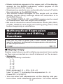
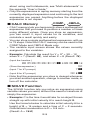
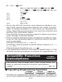
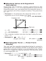
E
fx-570MS
fx-991MS
User’s Guide 2
(Additional Functions)
http://world.casio.com/edu_e/
CA 310030-001V08
Important!
Please keep your manual and all information handy for
future reference.
CASIO ELECTRONICS CO., LTD.
Unit 6, 1000 North Circular Road,
London NW2 7JD, U.K.
Contents
Before getting started... .......................... 3
kModes .................................................................... 3
Mathematical Expression Calculations
and Editing Functions ............................ 4
kReplay Copy .......................................................... 4
kCALC Memory ....................................................... 5
kSOLVE Function .................................................... 5
Scientific Function Calculations ............ 6
kInputting Engineering Symbols .............................. 6
Complex Number Calculations .............. 8
kAbsolute Value and Argument Calculation ............. 9
kRectangular Form ↔ Polar Form Display .............. 9
kConjugate of a Complex Number ........................ 10
Base-n Calculations .............................. 10
Statistical Calculations ......................... 12
Normal Distribution .................................................. 12
Differential Calculations ....................... 13
Integration Calculations ....................... 14
Matrix Calculations ............................... 15
kCreating a Matrix .................................................
kEditing the Elements of a Matrix ..........................
kMatrix Addition, Subtraction, and Multiplication ...
kCalculating the Scalar Product of a Matrix ...........
kObtaining the Determinant of a Matrix .................
kTransposing a Matrix ...........................................
kInverting a Matrix .................................................
kDetermining the Absolute Value of a Matrix .........
E-1
15
16
16
16
17
17
18
18
Vector Calculations ............................... 18
kCreating a Vector .................................................
kEditing Vector Elements .......................................
kAdding and Subtracting Vectors ..........................
kCalculating the Scalar Product of a Vector ..........
kCalculating the Inner Product of Two Vectors ......
kCalculating the Outer Product of Two Vectors .....
kDetermining the Absolute Value of a Vector ........
19
19
19
20
20
21
21
Metric Conversions ............................... 22
Scientific Constants .............................. 23
Power Supply ........................................ 25
Specifications ........................................ 27
See the “fx-95MS/fx-100MS/fx-115MS/fx-570MS/fx-991MS
User’s Guide” for details about the following items.
Removing and Replacing the Calculator’s Cover
Safety Precautions
Handling Precautions
Two-line Display
Before getting started... (except for “Modes”)
Basic Calculations
Memory Calculations
Scientific Function Calculations
Equation Calculations
Statistical Calculations
Technical Information
E-2
Before getting started...
k Modes
Before starting a calculation, you must first enter the correct
mode as indicated in the table below.
• The following table shows the modes and required
operations for the fx-570MS and fx-991MS.
fx-570MS and fx-991MS Modes
To perform this type of
calculation:
Basic arithmetic
calculations
Complex number
calculations
Standard deviation
Regression calculations
Base-n calculations
Solution of equations
Matrix calculations
Vector calculations
Perform this
key operation:
To enter
this mode:
F1
COMP
F2
CMPLX
FF1
FF2
FF3
FFF1
FFF2
FFF3
SD
REG
BASE
EQN
MAT
VCT
• Pressing the F key more than three times displays
additional setup screens. Setup screens are described
where they are actually used to change the calculator
setup.
• In this manual, the name of the mode you need to enter
in order to perform the calculations being described is
indicated in the main title of each section.
Example:
Complex Number
Calculations
CMPLX
Note!
• To return the calculation mode and setup to the initial
defaults shown below, press A B 2(Mode) =.
Calculation Mode:
Angle Unit:
Exponential Display Format:
Complex Number Display Format:
Fraction Display Format:
Decimal Point Character:
E-3
COMP
Deg
Norm 1, Eng OFF
a+b i
a b/c
Dot
• Mode indicators appear in the upper part of the display,
except for the BASE indicators, which appear in the
exponent part of the display.
• Engineering symbols are automatically turned off while
the calculator is the BASE Mode.
• You cannot make changes to the angle unit or other
display format (Disp) settings while the calculator is in
the BASE Mode.
• The COMP, CMPLX, SD, and REG modes can be used
in combination with the angle unit settings.
• Be sure to check the current calculation mode (SD, REG,
COMP, CMPLX) and angle unit setting (Deg, Rad, Gra)
before beginning a calculation.
Mathematical Expression
Calculations and Editing
Functions
COMP
Use the F key to enter the COMP Mode when you
want to perform mathematical expression calculations
or edit expressions.
COMP ............................................................ F 1
k Replay Copy
Replay copy lets you recall multiple expressions from replay
so they are connected as a multi-statement on the screen.
• Example:
Replay memory contents:
1+1
2+2
3+3
4+4
5+5
6+6
Multi-statement: 4 + 4:5 + 5:6 + 6
Use [ and ] to display the expression 4 + 4.
Press A [(COPY).
• You can also edit expressions on the display and perform other multi-statement operations. For more details
E-4
about using multi-statements, see “Multi-statements” in
the separate “User’s Guide.”
• Only the expressions in replay memory starting from the
currently displayed expression and continuing to the last
expression are copied. Anything before the displayed
expression is not copied.
COMP
k CALC Memory
CMPLX
• CALC memory lets you temporarily store a mathematical
expression that you need to perform a number of times
using different values. Once you store an expression,
you can recall it, input values for its variables, and
calculate a result quickly and easily.
• You can store a single mathematical expression, with up
to 79 steps. Note that CALC memory can be used in the
COMP Mode and CMPLX Mode only.
• The variable input screen shows the values currently
assigned to the variables.
• Example: Calculate the result for Y = X2 + 3X – 12
when X = 7 (Result: 58 ), and when X = 8 (Result: 76 ).
(Input the function.)
p y p u p x K + 3 p x , 12
C
(Input 7 for X? prompt.)
7=
(Input 8 for X? prompt.)
C8=
(Store the expression.)
• Note that the expression you store is cleared whenever
you start another operation, change to another mode, or
turn off the calculator.
k SOLVE Function
The SOLVE function lets you solve an expression using
variable values you want, without the need to transform or
simply the expression.
• Example: C is the time it would take for an object thrown
straight up with initial velocity A to reach height B.
Use the formula below to calculate initial velocity A for a
height of B = 14 meters and a time of C = 2 seconds.
Gravitational acceleration is D = 9.8 m/s2.
(Result: A = 16.8 )
E-5
B AC –
(B?)
(A?)
(C?)
(D?)
(A?)
1
DC 2
2
p2pup1-pk,
R1\2T-ph-pkK
AI
14 =
]
2=
9l8=
[[
AI
• Since the SOLVE function uses Newton’s Method, certain initial values (assumed values) can make it impossible to obtain solutions. In this case, try inputting another value that you assume to be near the solution and
perform the calculation again.
• The SOLVE function may be unable to obtain a solution,
even though a solution exists.
• Due to certain idiosyncrasies of Newton’s method, solutions for the following types of functions tend to be difficult to calculate.
Periodic functions (i.e. y = sin x)
Functions whose graph produce sharp slopes (i.e. y =
ex, y = 1/x)
Discontinuous functions (i.e. y = x )
• If an expression does not include an equals sign (=), the
SOLVE function produces a solution for expression = 0.
Scientific Function
Calculations
COMP
Use the F key to enter the COMP Mode when you
want to perform scientific function calculations.
COMP ............................................................ F 1
k Inputting Engineering Symbols
COMP
EQN
CMPLX
• Turning on engineering symbols makes it possible for
you to use engineering symbols inside your calculations.
E-6
• To turn engineering symbols on and off, press the F
key a number of times until you reach the setup screen
shown below.
Disp
1
• Press 1. On the engineering symbol setting screen that
appears, press the number key ( 1 or 2) that corresponds to the setting you want to use.
1(Eng ON): Engineering symbols on (indicated by
“Eng” on the display)
2(Eng OFF): Engineering symbols off (no “Eng”
indicator)
• The following are the nine symbols that can be used
when engineering symbols are turned on.
To input this symbol: Perform this key operation:
Ak
k (kilo)
M (Mega)
AM
G (Giga)
Ag
T (Tera)
At
m (milli)
Am
µ (micro)
AN
n (nano)
An
p (pico)
Ap
f (femto)
Af
Unit
103
106
109
1012
10–3
10–6
10–9
10–12
10–15
• For displayed values, the calculator selects the engineering symbol that makes the numeric part of the value fall
within the range of 1 to 1000.
• Engineering symbols cannot be used when inputting fractions.
• Example: 9 10 = 0.9 m (milli)
Eng
F ..... 1(Disp) 1
9 \ 10 =
0.
9 ⫼1
m
900.
When engineering symbols are turned on, even standard (non-engineering)
calculation results are displayed using engineering symbols.
E-7
AP
J
Complex Number
Calculations
0.9
9 ⫼1
m
900.
CMPLX
Use the F key to enter the CMPLX Mode when you
want to perform calculations that include complex
numbers.
CMPLX ........................................................... F 2
• The current angle unit setting (Deg, Rad, Gra) affects
CMPLX Mode calculations. You can store an expression in CALC memory while in the CMPLX Mode.
• Note that you can use variables A, B, C, and M only in
the CMPLX Mode. Variables D, E, F, X, and Y are used
by the calculator, which frequently changes their values.
You should not use these variables in your expressions.
• The indicator “R↔I” in the upper right corner of a
calculation result display indicates a complex number
result. Press A r to toggle the display between the
real part and imaginary part of the result.
• You can use the replay function in the CMPLX Mode.
Since complex numbers are stored in replay memory in
the CMPLX Mode, however, more memory than normal
is used up.
• Example: (23 i)(45 i) 68 i
(Real part 6)
2+3i+4+5i=
Ar
(Imaginary part 8 i)
E-8
k Absolute Value and Argument
Calculation
Supposing the imaginary number expressed by the
rectangular form z = a + bi is represented as a point in the
Gaussian plane, you can determine the absolute value (r)
and argument (␪ ) of the complex number. The polar form
is r⬔␪.
• Example 1: To determine the absolute value (r) and
argument (␪) of 3+4i (Angle unit: Deg)
(r = 5, ␪ = 53.13010235°)
Imaginary axis
Real axis
(r 5 )
(␪ 53.13010235 °)
AAR3+4iT=
AaR3+4iT=
• The complex number can also be input using the polar
form r⬔␪.
• Example 2:
2 ⬔ 45 1 i
(Angle unit: Deg)
L 2 A Q 45 =
Ar
k Rectangular Form ↔ Polar Form
Display
You can use the operation described below to convert a
rectangular form complex number to its polar form, and a
polar form complex number to its rectangular form. Press
A r to toggle the display between the absolute value
(r) and argument (␪ ).
• Example: 1 i ↔ 1.414213562 ⬔ 45
1+iAY=Ar
L 2 A Q 45 A Z = A r
(Angle unit: Deg)
E-9
• You select rectangular form (a+bi) or polar form (r⬔␪ )
for display of complex number calculation results.
F... 1(Disp) r
1(a+bi):Rectangular form
2(r⬔␪): Polar form (indicated by “r⬔␪ ” on the display)
k Conjugate of a Complex Number
For any complex number z where z = a+bi, its conjugate
(z) is z = a – bi.
• Example: To determine the conjugate of the complex
number 1.23 + 2.34i (Result: 1.23 – 2.34 i )
A S R 1 l 23 + 2 l 34 i T =
Ar
Base-n Calculations
BASE
Use the F key to enter the BASE Mode when you
want to perform calculations using Base-n values.
BASE ........................................................ F F 3
• In addition to decimal values, calculations can be
performed using binary, octal and hexadecimal values.
• You can specify the default number system to be applied
to all input and displayed values, and the number system
for individual values as you input them.
• You cannot use scientific functions in binary, octal,
decimal, and hexadecimal calculations. You cannot input
values that include decimal part and an exponent.
• If you input a value that includes a decimal part, the unit
automatically cuts off the decimal part.
• Negative binary, octal, and hexadecimal values are
produced by taking the two’s complement.
E-10
• You can use the following logical operators between
values in Base-n calculations: and (logical product), or
(logical sum), xor (exclusive or), xnor (exclusive nor),
Not (bitwise complement), and Neg (negation).
• The following are the allowable ranges for each of the
available number systems.
1000000000 ⬉ x ⬉ 1111111111
0 ⬉ x ⬉ 0111111111
Octal
4000000000 ⬉ x ⬉ 7777777777
0 ⬉ x ⬉ 3777777777
Decimal
–2147483648 ⬉ x ⬉ 2147483647
Hexadecimal
80000000 ⬉ x ⬉
FFFFFFFF
0⬉x⬉
7FFFFFFF
Binary
• Example 1: To perform the following calculation and
produce a binary result:
101112 110102 1100012
tb
Binary mode:
0.
b
10111 + 11010 =
• Example 2: To perform the following calculation and
produce an octal result:
76548
÷ 1210 5168
Octal mode:
to
0.
o
l l l 4 (o) 7654 \
l l l 1 (d) 12 =
• Example 3: To perform the following calculation and
produce a hexadecimal and a decimal result:
12016 or 11012 12d16 30110
Hexadecimal mode:
th
120 l 2 (or)
l l l 3 (b) 1101 =
Decimal mode:
K
E-11
0.
H
• Example 4: To convert the value 2210 to its binary, octal, and hexadecimal equivalents.
(101102 , 268 , 1616 )
tb
0.
b
l l l 1(d) 22 =
10110.
b
Octal mode:
o
26.
o
Hexadecimal mode:
h
16.
H
Binary mode:
• Example 5: To convert the value 51310 to its binary
equivalent.
tb
0.
l l l 1(d) 513 =
Ma t h ERROR
Binary mode:
b
b
• You may not be able to convert a value from a number
system whose calculation range is greater than the calculation range of the resulting number system.
• The message “Math ERROR” indicates that the result
has too many digits (overflow).
SD
Statistical
Calculations
REG
SD
Normal Distribution
Use the F key to enter the SD Mode when you want
to perform a calculation involving normal distribution.
SD ........................................................... F F 1
• In the SD Mode and REG Mode, the | key operates as
the S key.
• Press A D, which produces the screen shown below.
P ( Q ( R ( →t
1 2
3
E-12
4
• Input a value from 1 to 4 to select the probability
distribution calculation you want to perform.
P(t)
Q(t)
R(t)
• Example: To determine the normalized variate (→ t) for
x = 53 and normal probability distribution P(t) for the
following data: 55, 54, 51, 55, 53, 53, 54, 52
(→t = 0.284747398, P(t) = 0.38974 )
55 S 54 S 51 S 55 S
53 S S 54 S 52 S
53 A D 4(→t) =
A D 1( P( ) D 0.28 F =
Differential
Calculations
COMP
The procedure described below obtains the derivative of
a function.
Use the F key to enter the COMP Mode when you
want to perform a calculation involving differentials.
COMP ............................................................ F 1
• Three inputs are required for the differential expression:
the function of variable x, the point (a) at which the differential coefficient is calculated, and the change in
x (∆x).
A J expression P a P ∆x T
• Example: To determine the derivative at point x = 2 for
the function y = 3x2– 5x + 2, when the increase or decrease in x is ∆x = 2 × 10–4 (Result: 7 )
AJ3pxK,5px+2P2P
2eD4T=
E-13
• You can omit input of ∆x, if you want. The calculator
automatically substitutes an appropriate value for ∆x if
you do not input one.
• Discontinuous points and extreme changes in the value
of x can cause inaccurate results and errors.
• Select Rad (Radian) for the angle unit setting when
performing trigonometric function differential calculations.
Integration
Calculations
COMP
The procedure described below obtains the definite integral
of a function.
Use the F key to enter the COMP Mode when you
want to perform integration calculations.
COMP ............................................................ F 1
• The following four inputs are required for integration
calculations: a function with the variable x; a and b, which
define the integration range of the definite integral; and
n, which is the number of partitions (equivalent to N =
2n) for integration using Simpson’s rule.
d expression P a P b P n F
• Example:
∫ 15 (2x2 + 3x + 8) dx = 150.6666667
(Number of partitions n = 6)
d2pxK+3px+
8P1P5P6T=
Note!
• You can specify an integer in the range of 1 to 9 as the
number of partitions, or you can skip input of the number
of partitions entirely, if you want.
• Internal integration calculations may take considerable
time to complete.
• Display contents are cleared while an integration
calculation is being performed internally.
• Select Rad (Radian) for the angle unit setting when
performing trigonometric function integration calculations.
E-14
Matrix Calculations
MAT
The procedures in this section describe how to create
matrices with up to three rows and three columns, and
how to add, subtract, multiply, transpose and invert
matrices, and how to obtain the scalar product,
determinant, and absolute value of a matrix.
Use the F key to enter the MAT Mode when you want
to perform matrix calculations.
MAT ..................................................... F F F 2
Note that you must create one or more matrices before
you can perform matrix calculations.
• You can have up to three matrices, named A, B, and C,
in memory at one time.
• The results of matrix calculations are stored automatically
into MatAns memory. You can use the matrix in MatAns
memory in subsequent matrix calculations.
• Matrix calculations can use up to two levels of the matrix
stack. Squaring a matrix, cubing a matrix, or inverting a
matrix uses one stack level. See “Stacks” in the separate
“User’s Guide” for more information.
k Creating a Matrix
To create a matrix, press A j 1(Dim), specify a matrix
name (A, B, or C), and then specify the dimensions
(number of rows and number of columns) of the matrix.
Next, follow the prompts that appear to input values that
make up the elements of the matrix.
Ma t A 2 3
2 rows and 3 columns
You can use the cursor keys to move about the matrix in
order to view or edit its elements.
To exit the matrix screen, press t.
E-15
k Editing the Elements of a Matrix
Press A j 2(Edit) and then specify the name (A, B, or
C) of the matrix you want to edit to display a screen for
editing the elements of the matrix.
k Matrix Addition, Subtraction, and
Multiplication
Use the procedures described below to add, subtract,
and multiply matrices.
1 2
• Example: To multiply Matrix A = 4 0 by
–2 5
[ ]
[
Matrix B = –1 0 3
2 –4 1
(Matrix A 32)
(Element input) 1
(Matrix B 23)
]
([
3 –8 5
–4 0 12
12 –20 –1
])
A j 1(Dim) 1(A) 3 = 2 =
=2=4=0=D2=5=t
A j 1(Dim) 2(B) 2 = 3 =
(Element input)
D1=0=3=2=D4=1=t
(MatAMatB)
A j 3(Mat) 1(A) A j 3(Mat) 2(B) =
• An error occurs if you try to add, subtract matrices whose
dimensions are different from each other, or multiply a
matrix whose number of columns is different from that of
the matrix by which you are multiplying it.
k Calculating the Scalar Product of a
Matrix
Use the procedure shown below to obtain the scalar
product (fixed multiple) of a matrix.
• Example: Multiply Matrix C =
E-16
[
2 –1
–5 3
]
by 3.
([
])
6 –3
–15 9
(Matrix C 22)
A j 1 (Dim) 3(C) 2 = 2 =
(Element input)
2=D1=D5=3=t
3 - A j 3(Mat) 3(C) =
(3MatC)
k Obtaining the Determinant of a Matrix
You can use the procedure below to determine the
determinant of a square matrix.
• Example: To obtain the determinant of
2 –1 6
Matrix A =
5 0 1 (Result: 73 )
3 2 4
[
A j 1(Dim) 1(A) 3 = 3 =
(Matrix A 33)
(Element input)
]
2=D1=6=5=0=1=
3=2=4=t
A j r 1(Det)
A j 3(Mat) 1(A) =
(DetMatA)
• The above procedure results in an error if a non-square
matrix is specified.
k Transposing a Matrix
Use the procedure described below when you want to
transpose a matrix.
5 7 4
• Example: To transpose Matrix B =
8 9 3
5 8
7 9
4 3
[
([ ])
]
(Matrix B 23)
A j 1(Dim) 2(B) 2 = 3 =
(Element input)
5=7=4=8=9=3=t
(TrnMatB)
A j r 2(Trn)
A j 3(Mat) 2(B) =
E-17
k Inverting a Matrix
You can use the procedure below to invert a square matrix.
• Example: To invert Matrix C =
([
–0.4 1 –0.8
–1.5 0.5 –1.5
–0.8 0 –0.6
])
[
–3 6 –11
3 –4 6
4 –8 13
]
(Matrix C 33)
A j 1(Dim) 3(C) 3 = 3 =
(Element input)
D 3 = 6 = D 11 = 3 = D 4 =
6 = 4 = D 8 = 13 = t
A j 3(Mat) 3(C) a =
(MatC –1)
• The above procedure results in an error if a non-square
matrix or a matrix for which there is no inverse
(determinant = 0) is specified.
k Determining the Absolute Value of a
Matrix
You can use the procedure described below to determine
the absolute value of a matrix.
• Example: To determine the absolute value of the matrix
produced by the inversion in the previous example.
([
(AbsMatAns)
0.4
1 0.8
1.5 0.5 1.5
0.8
0 0.6
])
A A A j 3(Mat) 4(Ans) =
Vector Calculations
VCT
The procedures in this section describe how to create a
vector with a dimension up to three, and how to add, subtract, and multiply vectors, and how to obtain the scalar
product, inner product, outer product, and absolute value
of a vector. You can have up to three vectors in memory at
one time.
E-18
Use the F key to enter the VCT Mode when you want
to perform vector calculations.
VCT ..................................................... F F F 3
Note that you must create one or more vector before you
can perform vector calculations.
• You can have up to three vectors, named A, B, and C, in
memory at one time.
• The results of vector calculations are stored automatically
into VctAns memory. You can use the matrix in VctAns
memory in subsequent vector calculations.
k Creating a Vector
To create a vector, press A z 1 (Dim), specify a vector name (A, B, or C), and then specify the dimensions of
the vector. Next, follow the prompts that appear input values that make up the elements of the vector.
Vector name
Vc t A1
Dimensions of vector
0.
Arrow indicates
direction you should
scroll to view other
elements.
Element value
You can use the e and r keys to move about the vector in order to view or edit its elements.
To exit the vector screen, press t.
k Editing Vector Elements
Press A z 2(Edit) and then specify the name (A, B,
C) of the vector you want to edit to display a screen for
editing the elements of the vector.
k Adding and Subtracting Vectors
Use the procedures described below to add and subtract
vectors.
E-19
• Example: To add Vector A = (1 –2 3) to Vector B = (4 5
–6). (Result: (5 3 –3) )
(3-dimensional Vector A)
(Element input)
(3-dimensional Vector B)
(Element input)
(VctA + VctB)
A z 1(Dim) 1(A) 3 =
1=D2=3=t
A z 1(Dim) 2(B) 3 =
4=5=D6=t
A z 3(Vct) 1(A) +
A z 3(Vct) 2(B) =
• An error occurs in the above procedure if you specify
vectors of different dimensions.
k Calculating the Scalar Product of
a Vector
Use the procedure shown below to obtain the scalar
product (fixed multiple) of a vector.
• Example: To multiply Vector C = (–7.8 9) by 5.
(Result: (–39 45) )
(2-dimensional Vector C)
(Element input)
(5VctC)
A z 1(Dim) 3(C) 2 =
D7l8=9=t
5 - A z 3(Vct) 3(C) =
k Calculating the Inner Product of
Two Vectors
Use the procedure described below to obtain the inner
product ( ) for two vectors.
⋅
• Example: To calculate the inner product of Vector A and
Vector B
(Result: – 24 )
⋅
(VctA VctB)
A z 3(Vct) 1(A)
A z r 1(Dot)
A z 3(Vct) 2(B) =
• An error occurs in the above procedure if you specify
vectors of different dimensions.
E-20
k Calculating the Outer Product of
Two Vectors
Use the procedure described below to obtain the outer
product for two vectors.
• Example: To calculate the outer product of Vector A and
Vector B
(Result: (–3, 18, 13) )
A z 3(Vct) 1(A) A z 3(Vct) 2(B) =
(VctAVctB)
• An error occurs in the above procedure if you specify
vectors of different dimensions.
k Determining the Absolute Value of
a Vector
Use the procedure shown below to obtain the absolute
value (size) of a vector.
• Example: To determine the absolute value of Vector C
(Result: 11.90965994 )
A A A z 3(Vct) 3(C) =
(AbsVctC)
• Example: To determine the size of the angle (angle unit:
Deg) formed by vectors A = (–1 0 1) and B = (1 2 0), and
the size 1 vector perpendicular to both A and B.
(Result: 108.4349488 °)
cos ␪ (A ⋅B)
(A B)
, which becomes ␪ cos–1 ⋅
A B
A B
Size 1 vector perpendicular to both A and B (3-dimensional Vector A)
A z 1(Dim) 1(A) 3 =
D1=0=1=t
(Element input)
(3-dimensional Vector B)
A z 1(Dim) 2(B) 3 =
1=2=0=t
(Element input)
⋅
(VctA VctB)
AB
AB
A z 3(Vct) 1(A) A z r 1(Dot)
A z 3(Vct) 2(B) =
E-21
(Ans(AbsVctAAbsVctB))
\ R A A A z 3(Vct) 1(A)
- A A A z 3(Vct) 2(B) T =
(cos–1Ans) (Result: 108.4349488 °)
AVg=
(VctAVctB)
A z 3(Vct) 1(A) A z 3(Vct) 2(B) =
(AbsVctAns)
A A A z 3(Vct) 4(Ans) =
(VctAnsAns)
(Result: (– 0.666666666 0.333333333 – 0.666666666) )
A z 3(Vct) 4(Ans) \ g =
Metric Conversions
COMP
Use the F key to enter the COMP Mode when you
want to perform metric conversions.
COMP ............................................................ F 1
• A total of 20 different conversion pairs are built-in to
provide quick and easy conversion to and from metric
units.
• See the Conversion Pair Table for a complete list of
available conversion pairs.
• When inputting a negative value, enclose it within parentheses R , T .
• Example: To convert –31 degrees Celsius to Fahrenheit
R D 31 T A c 38 =
( –3 1 )
°C °F
– 23.8
38 is the Celsius-to-Fahrenheit conversion pair number.
E-22
u Conversion Pair Table
Based on NIST Special Publication 811 (1995).
To perform
this conversion:
Input this
pair number:
To perform
this conversion:
Input this
pair number:
in → cm
cm → in
ft → m
m → ft
yd → m
m → yd
mile → km
km → mile
n mile → m
m → n mile
acre → m2
m2 → acre
r
gal (US) →r
r → gal (US)
r
gal (UK) →r
r → gal (UK)
pc → km
km → pc
km/h → m/s
m/s → km/h
01
02
03
04
05
06
07
08
09
10
11
12
13
14
15
16
17
18
19
20
oz → g
g → oz
lb → kg
kg → lb
atm → Pa
Pa → atm
mmHg → Pa
Pa → mmHg
hp → kW
kW → hp
kgf/cm2→ Pa
Pa → kgf/cm2
kgf•m → J
J → kgf•m
lbf/in2 → kPa
kPa → lbf/in2
°F → °C
C → °F
J → cal
cal → J
21
22
23
24
25
26
27
28
29
30
31
32
33
34
35
36
37
38
39
40
Scientific Constants
COMP
Use the F key to enter the COMP Mode when you
want to perform calculations using scientific constants.
COMP ............................................................ F 1
• A total of 40 commonly-used scientific constants, such
as the speed of light in a vacuum and Planck’s constant
are built-in for quick and easy lookup whenever you need
them.
E-23
• Simply input the number that corresponds to the scientific
constant you want to look up and it appears instantly on
the display.
• See the Scientific Constant Table for a complete list of
available constants.
• Example: To determine how much total energy a person
weighing 65kg has (E = mc2 = 5.841908662 × 1018 )
65 L 28 K =
65 Co 2
5.841908662 18
28 is the “speed of light in vacuum” constant number.
u Scientific Constant Table
Based on ISO Standard (1992) data and CODATA recommended values (1998).
To select this constant:
proton mass (mp)
neutron mass (mn)
electron mass (me)
muon mass (mµ)
Bohr radius (a0)
Planck constant (h)
nuclear magneton (µN)
Bohr magneton (µ B)
Planck constant, rationalized ( )
fine-structure constant (α)
classical electron radius (re)
Compton wavelength (λ c)
proton gyromagnetic ratio (γ p)
proton Compton wavelength (λ cp)
neutron Compton wavelength (λ cn)
Rydberg constant (R∞)
atomic mass unit (u)
proton magnetic moment (µ p)
electron magnetic moment (µ e)
neutron magnetic moment (µ n)
muon magnetic moment (µ µ )
Faraday constant (F)
elementary charge (e)
Avogadro constant (NA)
Boltzmann constant (k)
E-24
Input this scientific
constant number:
01
02
03
04
05
06
07
08
09
10
11
12
13
14
15
16
17
18
19
20
21
22
23
24
25
To select this constant:
molar volume of ideal gas (Vm)
molar gas constant (R)
speed of light in vacuum (C 0)
first radiation constant (C 1)
second radiation constant (C 2)
Stefan-Boltzmann constant (σ)
electric constant (ε 0)
magnetic constant (µ 0)
magnetic flux quantum (φ 0)
standard acceleration of gravity (g)
conductance quantum (G 0)
characteristic impedance of vacuum (Z 0)
Celsius temperature (t)
Newtonian constant of gravitation (G)
standard atmosphere (atm)
Input this scientific
constant number:
26
27
28
29
30
31
32
33
34
35
36
37
38
39
40
Power Supply
The type of battery you should use depends on the model
number of your calculator.
fx-991MS
The TWO WAY POWER system actually has two power
supplies: a solar cell and a G13 Type (LR44) button battery.
Normally, calculators equipped with a solar cell alone can
operate only when relatively bright light is present. The
TWO WAY POWER system, however, lets you continue
to use the calculator as long as there is enough light to
read the display.
• Replacing the Battery
Either of the following symptoms indicates battery power
is low, and that the battery should be replaced.
• Display figures are dim and difficult to read in areas
where there is little light available.
• Nothing appears on the display when you press the
5 key.
E-25
u To replace the battery
Screw
Screw
1 Remove the five screws that
hold the back cover in place
and then remove the back
cover.
2 Remove the old battery.
3 Wipe off the sides of new
battery with a dry, soft cloth.
Load it into the unit with the
positive k side facing up (so
you can see it).
4 Replace the back cover and secure it in place with the
five screws.
5 Press 5 to turn power on. Be sure not to skip this
step.
fx-570MS
This calculator is powered by single G13 Type (LR44)
button battery.
• Replacing the Battery
Dim figures on the display of the calculator indicate that
battery power is low. Continued use of the calculator
when the battery is low can result in improper operation.
Replace the battery as soon as possible when display
figures become dim.
• To replace the battery
1 Press A i to turn off power.
2 Remove the screw that holds
the battery cover in place and
then remove the battery cover.
3 Remove the old battery.
4 Wipe off the sides of new
battery with a dry, soft cloth.
Load it into the unit with the
positive k side facing up (so
you can see it).
E-26
Screw
5 Replace the battery cover and secure it in place with
the screw.
6 Press 5 to turn power on.
Auto Power Off
Calculator power automatically turns off if you do not
perform any operation for about six minutes. When this
happens, press 5 to turn power back on.
Specifications
Power Supply:
fx-570MS: Single G13 Type button battery (LR44)
fx-991MS: Solar cell and a single G13 Type button
battery (LR44)
Battery Life:
fx-570MS: Approximately 9,000 hours continuous
display of flashing cursor.
Approximately 3 years when left with power
turned off.
fx-991MS: Approximately 3 years (1 hour use per day).
Dimensions: 12.7 (H) 78 (W) 154.5 (D) mm
1/2⬙ (H) 31/16⬙ (W) 61/16⬙ (D)
Weight:
105 g (3.7 oz) including battery
Power Consumption: 0.0002 W
Operating Temperature: 0°C to 40°C (32°F to 104°F)
E-27
CASIO COMPUTER CO., LTD.
6-2, Hon-machi 1-chome
Shibuya-ku, Tokyo 151-8543, Japan
SA0403-F Printed in China