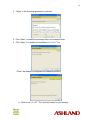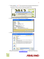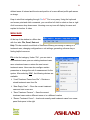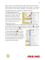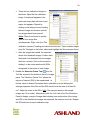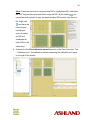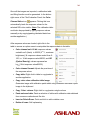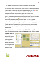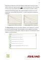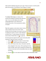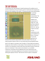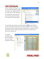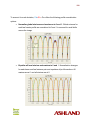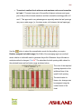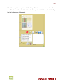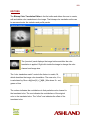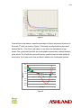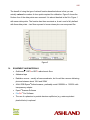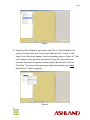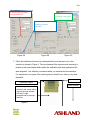
1
USER MANUAL FilmQA™ Pro Version: 3.0.4864.35322 Date: July 30, 2013 Advanced Specialty Ingredients 1361 Alps Road Wayne, NJ 07470 Table of Contents Introduction 1 Installation 2 Getting Started 7 Operations Menu Bar Case Description Case Data Selector Panel Image Panel Film Evaluation Panel 8 14 14 19 22 Processes Calibration Dose Map Plan to Dose Comparison One Scan Protocol 28 41 50 67 Physics Modules Star Shot Analysis Flatness and Symmetry Analysis Picket Fence Analysis 74 93 96 Editors Bitmap Color Translation Color Translation Map 103 104 Configuration Managing the Libraries 108 Appendices Calibration Protocol Efficient Protocol for Radiochromic Film Dosimetry (One Scan Protocol) Post-Exposure Change 113 122 131 Troubleshooting 110 Index 133 1 INTRODUCTION (Video: http://www.youtube.com/watch?v=A26tTy2iF88) FilmQA™ Pro is a sophisticated, quantitative, analysis tool specifically designed to simplify and streamline your IMRT QA process. The program allows you to scan or open images of exposed application films and calculate the optimized dose maps. The calculation is based on a scanner-dependent function generated from calibrated data derived from three color channels (red, green and blue). The three color channels are produced by using Gafchromic™ EBT2, EBT3, MD-V3 or HD-V2 films. These selfdeveloping radiochromic dosimetry films are intended specifically for applications in radiotherapy. FilmQA™ Pro complements Gafchromic™ dosimetry films. When these Gafchromic™ films are used, the optimized dose maps include corrections for thickness artifacts by using the blue color channel to measure the absorbance of the yellow marker-dye in the films and when the films are used with a professional flat-bed color scanner, FilmQA™ Pro’s easy-to-use features are ideal for the fast-paced, processor-less environment of the modern hospital. The purpose of this guide is to familiarize the user with the many useful features of FilmQA™ Pro with a particular focus on the basic functions of calibration, calculation of a dose map from an exposed film, comparison of a dose map to a patient-specific treatment plan and execution of machine QA functions like star shot analysis, flatness and symmetry determination and assessment of MLC function. In addition to the contents of this User Guide a number of instructional videos are available for view on YouTube. Use the table of contents in this guide to easily navigate to the desired section, or read through the instructions step-by-step. In the end, our goal is to provide both an in-depth introduction to and a quick reference for, all the features available in FilmQA™ Pro. FilmQA™ Pro is built on Ashland proprietary technology, patents pending. 2 INSTALLATION Recommended computer requirements for FilmQA™ Pro: Hardware: Processor: RAM: Graphics: Input Devices: Scanners: i7 8 GB, 1333 MHz UXGA+ (1600 x 1200), HD (1920 x 1080) or WQXGA (2560 x 1600) Keyboard and Mouse [Tablet (Touch screens) not supported] Epson 11000XL and 10000XL with Epson Twain Drivers Minimum computer requirements for FilmQA™ Pro: Hardware: Processor: RAM: Graphics: i5 4 GB, 1333 MHz Wide XGA+ (1440 x 990) XGA+ (1152 x 864) Software: Operating System: Windows 8 Windows 7 [with Microsoft® .NET Framework 4.0 – Full] Windows Vista [with Microsoft® .NET Framework 4.0 – Full] Windows XP [with Service Pack 3 (SP3), Microsoft® .NET Framework 4 – Full and Microsoft® Visual C++ 2010 Redistributable Package (x86)] 3 1. Download and run the installation file from www.filmqapro.com\install. 2. Navigate through the following prompts by hitting “Next>” 4 3. “Agree” to the licensing agreement to proceed 4. Click “Next>” to install the necessary files in the selected folder 5. Click “Next>” to complete the installation of FilmQA™ Pro “Close” the window to completed the installation process 6. Click on the “FilmQA™ Pro” shortcut located on your desktop 5 7. When starting FilmQA™ Pro for the first time, the program will prompt you to generate a license (see the following message below): 8. Click “Ok” and the following window will appear 9. Click “Save” and note the stored key file name and location 10. Email the saved file to [email protected] to obtain your license key 6 11. After receiving the license key, save the key to the application folder in either “c:\Program Files\ISP Advanced Materials\FilmQA Pro 20XX\” or “c:\Program Files\Ashland Advanced Materials\FilmQA Pro 20XX\”. NOTE: Only one (1) license key can be stored in the application folder.] 12. Return to the “FilmQA™ Pro” shortcut on your desktop and when you click the icon this time, FilmQA™ Pro will begin. 7 GETTING STARTED (Video: http://www.youtube.com/watch?v=5mAidqhL5qM) When FilmQA™ Pro loads, the following screen will appear: As you can see, there are three sections. To the left is the “Case Data Selector Panel” which allows you to add selected image objects from a saved file or directly from a scanner. This panel contains the case tree and its branches are a collection of the case objects required to execute a case. For instance to compare dose measurements to a patient-specific plan, the tree requires a Film Calibration Object, a Dose Map Object and a Dose-to-Plan Comparison Object. The objects added to the case tree are dependent on preceding objects. For example, a dose map object cannot function unless the case tree contains a calibration object. Click the “+” or “-“signs to expand or compress any branch of the tree. The center section or “Image Panel” displays the selected images. The section to the right the “Film Evaluation Panel” and displays the analytical data for the particular image in the “Image Panel”. The right hand window can also display properties of a selected image for example, its source, time stamp, image resolution, dose range, data statistics as well as the cursor position and location/size of all user- 8 defined areas of interest and the size and position of a user-defined profile path across an image. Keep in mind that navigating through FilmQA™ Pro is very easy. Using the keyboard and mouse point-and-click commands, you can either left click to select an item or right click to access a drop-down menu. Hovering over any icon will display its name and explain its function. A video MENU BAR At the top of the window is a Menu bar with four tabs: File, Panel, Data and Help. This bar controls a multitude of functions including the saving or loading of a treatment case, changing configuration or unit settings, generating a license key or finding helpful resources File is the first category. Under “File”, you can start a new treatment case, open an existing treatment case, save a treatment case or review the most recent treatment cases. Users can also configure certain parameters or change the unit of measurement for the system. After selecting “File”, the following choices are available: “Load Treatment Cases from File” – Retrieve a stored treatment case from file “New Empty Case” – Close the current treatment case and start a new one “Save Treatment Case as” – Save the current treatment case under a different name or in a different location “Recent Treatment Cases” – Load most recently used treatment cases from a new panel that opens to the right 9 “Configuration” – Loads/saves FilmQA™ Pro configuration settings from a new drop-down list “Auto Save” – Saves the configuration automatically each time you exit the application “Reload Last Case with Configuration” – Opens treatment case with the same configuration that was set the last time the case was opened. “Save File Locations” – Recalls location of saved files “Reset to Default” – Reset the configuration to system default. “Unit System” – Loads/saves the user’s unit preferences from a new panel “Auto Save” – Save the units automatically each time you exit the application “Load Unit Standards Only” – Load only “standard” units and exclude the loading of number formats “Exit” – Closes FilmQA™ Pro “Ask Before Exit” – Enables a ‘pop-up’ window asking whether to close FilmQA™ Pro when ‘Exit” button is clicked Panel is the next category and helps you configure the various tools utilized in FilmQA™ Pro. “Tool Management” allows you to select the tools available in the software. “Reset to Default Tools” will change the tool set back to the original factory configuration. “Always include Default Tools” is the option to see the default tools all the time. “Treatment Object Management” tailors the drop down menu selections. 10 “Object Type Management” displays the Case Object library allows various objects to be activated and therefore available from the drop down list in the Case Data Selector Panel. User-written functions can be added to the library. “Reset to Default Treatment Object Types” returns the object list back to default settings. “Always include Default Treatment Object Types” is the option to see the default object list all the time. “Add New Treatment Object Type of Read Cases” to import user-written treatment objects from other cases. “Dose Plan Reader Management” selects interfaces for specific treatment-planning software, e.g. Pinnacle, Brain Lab, Eclipse, etc. User-written functions can be added to the library. “Reader Type Management” allows various readers to be available in the drop down list. “Reset to Default Reader Types” returns the reader type list back to the default settings. Always include Default Reader Types” is the option to see the default reader types all the time. “Show Menu to Preselect Reader Type” is a setting which will always open a separate window to select the reader type. “Calibration Function Management” manages the selection of equations from a library of functions correlating film response with radiation dose User-written functions can be added to the library. “Reset to Default Calibration Function Types” returns the calibration function list back to default settings “Always include Default Calibration Function Types” is the option to see the default calibration equations all the time. “Case Data Selector Location” selects the position of the case data selector either left, top, right or bottom. 11 Data, as the name describes, includes all data related to the patient, treatment case or scanner. This tab also allows the changing of measurement units and adjustment of software preferences. “Patient Data” allows you to create a new patient and add or remove a patient from the database. “Treatment Case Data” allows you to create a new treatment case and add or remove a case from the database. “Scanner Data” allows you to add or remove a scanner from the database. “Units” allows you to change settings and format of units within the software. “Preferences” configures the appearance and layout of FilmQA™ Pro. “Tool Tip” shows or hides helpful information in the software ( hover the cursor over the icon or area of interest) “Padding” adjusts the amount of space around each section of the software. The range for the frame is between 0 and 50 pixels. Horizontal and vertical adjustments range from 1 to 20 pixels. “Fonts” allows you to choose between various character types and sizes. “Colors” adjusts the palette settings for the foreground, “Fore Color” and background, “Back Color”. “Preset Color Pairs” is another option to select 12 predetermined color mixes. Colors can always be returned to default settings by selecting “Reset to Default Colors” “Label Position” changes the location of icons and panel labels to either “Top Left”, “Top Center”, “Top Right”, “Bottom Left”, “Bottom Center” or “Bottom Right”. “Status Bar” is located at the bottom of the screen and does the following: 1. Informs you of the current software condition; 2. Allows changes to be made to the status history; 3. Allows you to configure FilmQA™ Pro (see “Preferences”); and 4. Provides you a means to copy a screen shot. A “right click” on the status bar allows for three possible choices: 1. “Clear Status” erases all information stored in the status bar. 2. “Auto Clear Status” sets the elapsed time before the information is automatically erased from the status bar. 3. “History” displays all messages in the status bar. “Exceptions” allows you to view the history of software exceptions, which are events the application could not complete. Exceptions” are a tool to aid in identifying and fixing software bugs. By “right clicking” inside the “Exception History” window, you can select: “Exception Level Depth” – the number of lines displayed related to that particular event “History Length” – The number of events allowed to view 13 “Reset History” – Clear all events “Word Wrap” – Wrap the words to fit the window width “Filter” (see arrow above) allows you to enter a criterion to reduce the number of visible exceptions in the window. See detailed descriptions and examples in “Menu”. “Status” shows the complete history of conditions since the application was opened. By “right clicking” in the window, options become available to either “Clear Status History”, “Copy All” line items or “Copy a Selected Row” 4. “Appearance” allows you to configure FilmQA™ Pro (see “Preferences”) 5. “Copy Screen Shot” is simply stated and copies an image of the current screen. 6. “Status Line Tool Tip” provides an overview of status history when moving the cursor to the “Status Bar” 7. The “On Exception Show Popup Message” option enables a popup window when an exception occurs. The “Task” button is an indicator located in lower right corner of the screen. When the application is idle, the icon will appear as look like similar to this otherwise the icon will . The number on the left indicates the number of calculation tasks in process. To cancel the current task, right click on the icon and select . File management is the last option under this heading. The option toggles onoff the ability to let FilmQAPro remember the last open file location, the last saved file location and to sync the last open and saved file locations. 14 Help is the last category and provides instructional information such as the user’s manual, license data generator, license expiration notification and related web links. “FilmQA Pro User’s Guide” is to view the user manual for the software. “Generate License Data” saves or copies the license data. For details on how to obtain a license key, see Installation (Page 4 – Step #8). “Notify, Before License Expires” monitors and warns the users before the license expires. Choices are for 1, 2, 7, 14, 21, 50 and 100 days. The default setting is 14 days. “Web Pages” are links to websites related to FilmQA™ Pro. “About FilmQA Pro 20xx” provides installation information on FilmQA™ Pro (i.e. Version Number, License ID, License Renewal Data, etc.) CASE DATA SELECTOR PANEL The Case Description is a default addition to the case tree. To store patient or case information, go to the Case Data Selector section and click the “+” sign next to “Case Description”. The tree will expand to show “Patient Data – Not Assigned” and “Case Data – Not Assigned”. “Patient Data” opens a drop down list to select an existing patient from the database. By choosing “None”, no information is necessary. “Edit Patient Data” allows the user to update patient information in the database. 15 “Case Data” opens a drop down list to select case specific information related to the patient. Double-click the icon to open the pop-up window and select the preferred case. “Patient Data” will change to match the patient name of the treatment case selected. Case Object Management allows objects to be added to the Case Tree to create a film dosimetry case. Under “Add New Case Object”: “Film Calibration (Ordinary)” – Scan or open a file containing a single image to generate a calibration curve “Film Calibration (Mosaic)” – Scan or open multiple image files to generate a calibration curve “Film Calibration Dose Maps” – Calculates a dose map, consistency map and uniformity map from the image or images used to generate the calibration curve “Images Only (Multiple Scans)” – Scan or open multiple image files. The images can be averaged or fused together and the resultant image can be saved or copied to be used as required. “Dose Map (Single Scan)” – Scan or open an image file for conversion to a dose map from a Film Calibration Object. A calibration curve is required in the Case Tree before a dose map can be generated. Note: By default the first Film Calibration Object in the case is used. In the Dose Map branch of the Case Tree select a different dependency if the case contains multiple Calibration Objects and one of the subsequent ones is to be used. “Dose to Plan Comparison” – Import a treatment plan from a file, TPS or DICOM and do a gamma analysis against a treatment film. A Dose map Object is required in the Case Tree before a dose-to-plan comparison can be done. Note: 16 By default the first Dose Map in the case is used. In the Dose-to-plan Comparison branch of the Case Tree select a different dependency if the case contains multiple Dose Map Objects and one of the subsequent ones is to be used. “MLC Star Shot Physics QA” – Scan or open a file of an image to perform a star shot analysis “MLC Picket Fence Physics QA” – Scan or open a file of an image to perform a picket fence analysis “Flatness and Symmetry Physics QA” – Scan or open multiple files of an image to perform beam uniformity analysis “Flatness and Symmetry Physics QA (Dose Map)” – Analyze a dose map generated from a scanned film or image file using of the calibration function of a Film Calibration Object. Note: By default the first Film Calibration Object in the case is used. In the Flatness and Symmetry Physics QA (Dose Map) branch of the Case Tree select a different dependency if the case contains multiple Calibration Objects and one of the subsequent ones is to be used. Under “<Open Case Object from File>” – Open a case object from file “New Treatment Case”, a drop down list provides options to select a template of objects to create a treatment case. “Dose to Plan Comparison” – Opens a template for a full treatment case that includes the following case objects: Film Calibration (Ordinary), Dose Map (Single Scan) and Dose to Plan Comparison. “<New (Empty) Case>” – Erases everything opened under “Case Data Selector” <Open Case Object from File>” – Open a case object from file 17 Case Data Selector shows the case management tree which allows you to add selected image objects into case data. It is located on the left side of the screen. The case data selector allows you to add patient information, calibration data, and film images and data analysis from a file or directly from a scanner. Remember each object added to the tree is dependent on the objects above it. At the foot of the panel are a number of icons: “Open” treatment cases from file “Save” treatment cases to the computer. All objects opened in the case data selector are saved as one case. “Expand” only the selected treatment object tree node. “Configure Twain Scanner” controls the scanner configuration “Select Twain Source” chooses the desired scanner. Select the appropriate scanner in the pop-up window. “Show Twain Parameter Panel before Each Scan” enables the scanner panel to open each time when scanning. “Twain Resolution” changes the spatial resolution of the scans. Choices are 36, 48, 60, 72, 96, 144 and 192 DPI. “Light Path” chooses between reflection and transmission modes on the scanner. “Auto Detect whether Scanner Rotates Image” enables software to rotate the image 90° to match the display with the scanner information. This feature is used 18 for some scanner drivers which would auto rotate the image without rotating the device information (e.g. Epson used in conjunction with Windows XP). “Detect whether Scanner Rotates Image” manually forces the detection of image rotation when the automatic feature is disabled. “Scanner Rotates Image” manually forces the scanner to rotate the displayed image 90°. “Options” displays a new window with various choices. Among others you can enable 24 bit rgb images (not recommended for film dosimetry) and “Allow any image resolution” Remember full-frame, high resolution images can get very large and slow down an analysis. 19 IMAGE PANEL Image Panel displays the image and user-defined regions of interest for dose calibration and measurement. It is located at the center of the screen. The image panel allows the users to view the active image and to select the region of interest (ROI) for dose calibration and calculation. Fifteen icons are designated as tools and appear on the bar to the left of the image panel. These tools are Selection Frame, Fiducial Management, Color Leveling, Pause, Image Scaling, Color Channel Selector, Color Range Spreader, Magnifier, Undo/Redo Buffer, Flip/Rotation, Cropping, Filtering, Color Translation, Image Exporter and Editor Configuration. Rightclicking on any tool opens a pop-up window of additional options. Selection Frame, allows you to select one or more regions of interest (rectangular, square, circular, elliptical) on the image displayed. Fiducial Management, allows you to select points of reference manually or turn-on an algorithm to automatically detect those reference regions on the image displayed. Color Leveling, allows you to adjust the brightness and contrast levels of the image displayed. Profile Path, Pause, Image Scaling, displays the path line when the Profile tab is enabled. allows you to stop all th eimage tools selected. allows you to select image coordinate system and axis units. When this tool is selected, you can change the coordinate system between the image or the scanner. This ability allows the user to compare scanner effects on the image easier. Selecting “options” allows the user to change the configuration of the axis, image grid and color of the scanner background when scanner coordinates are used. 20 Color Channel Selector, allows you to select, invert, or gray the color channels of the image displayed. Note: This tool does not change the bitmap of the image. The screen view only changes. Color Range Spreader, allows you to select a range of color channels to apply to the displayed image. “Option” available are: Delete Color Channel Scaling – to change the channel scaling back to full range Color Channel Scaling Dialog – opens the “color range” window so you can manually enter the minium and maximum values. The “lock button” makes the minimum and maximum values for all three chanells the same. Auto Scale Color Channels to range of Selected Frame – sets the image color channel range to color channels of the selected frame in real time. Scale Color Channels to Image Range – sets the color ranges to the ones of the displayed image. Magnifier, allows you to zoon in and out of the image. By clicking on the icon, one can scroll up to zoom in and scroll down to zoom out using the mouse. Auto Fit – fits the image atuomatically to your preference everytime the image is displayed in the “Image Panel”. Undo/Redo Buffer, Flip/Rotation, allows you to undo and redo the changes made to the image. allows you to flip or rotate the entire image or region of the current image selected. Cropping, allows you to crop the region of the image displayed. Filtering, filters the entire image or region of the image displayed by allowing pixel modifications using a filter matrix to combine surrounding pixels. To define and edit filters, open the filtering tool. Color Translation, allows you to translate colors of the entire image or region of image displayed. Equalize Color Channel – divides all color values by a normalized color value. For example when “Equalize Red” is selected, all color values are divided by the normalized red value. 21 Equalized Color Channel Density – divides all color channel densities by a normalized color density. For example when “Equalize Red Density” is selected, all color channel densities are divided by a normalized red density. Other options are to invert , translate or manage the color through densities or maps (See Bitmap Color Translation Editor and Color Translation Maps Editor). Image Exporter, , allows you to export to a file or clipboard the entire image, the image with color channel selected or region of the image displayed. Editor Configuration, , allows you to adjust the configuration of the editor (i.e. enable icons, adjust axis, etc.) 22 FILM EVALUATION PANEL Film Evaluation Panel or “Analysis Window” displays evaluation data for any image or dose map in the Image Panel. The panel has tabs to access eight sub-panels: Info, Cursor, Statistics, Profile, Contour, Iso-map, Surface and Report. Info Panel displays information pertaining to the image (i.e. size, pixel, resolution, and color channel range, memory and scanner information) as well as the sizes and locations of any areas of interest displayed on the image. Right-click in the panel to change the units of measurement. Cursor Panel displays information from the red dashed box area overlaid on the image - see red arrow below. In the red box, the pixel statistics shows the information contained in the red dashed box (look for red arrow to the right). Right click in the area outlined in red to change the units of measurement. In the yellow box, the window displays an enlarged image of the red dashed box in the Image Panel. Move the pointer to see the location, magnification percentage and color range in the cursor area. The slide bar at the bottom of the window changes the magnification of the image. The higher the magnification, the smaller the red dashed box. Increase magnification by dragging the bar to the right. 23 The color channel spreader, spreads the color so that the selected image region is displayed with a color saturation between 0% and 100%. This feature magnifies differences in color. The color channel selector, selects the combination of red, green and blue color channels for mapping the view of the image region. Statistics Panel shows the dose histogram and the image statistics. Information is displayed for the entire image as well as the image around the cursor. In addition information is displayed for any areas of interest marked on the image. It displays the image statistics all the areas in tabular form and of the full frame or a highlighted area of interest in histogram form. Use the window at the bottom of the panel to select the histogram displayed. Move the cursor or area of interest around to see the real time tracking of pixel information in the “Cursor Region” column or frame columns. Pixel statistics (#, #) at the bottom of the panel indicates the location of the cursor. The two arrows, or number format buttons, can change the format of the numbers displayed in the window. Depending on the image selected from the Case Tree in the Case Data Selector, the table will present information related to the color channel (film image) or dose for the color channel (dose map image). Right click inside the table to: change the units and format of the column; copy the table; change the pixels of cursor region or 4) change the configuration of the table. The histogram shows the bar graph for probability versus dose or color channel response. To zoom in, click and drag a region from top left to bottom right of the preferred 24 region. To pan out, click and drag from bottom right to top left. Right click and hold to drag the histogram across the data range. Right click inside the graph to: 1) change the units and format for the color channel or probability, 2) copy the table or chart, 3) set a new predefined data range or 4) change the configuration of the graph. The image histogram region dropdown list selects the region of the image displayed in the histogram. Right click inside the window and check “simple frame unions” to add data of all frames (counts possible overlap regions multiple times). Uncheck the option to count overlap regions only once. The histogram range button lets you toggle between full histogram range (0-100%) and auto range (i.e. the zero clusters at boundaries are removed). The when full range is on and becomes when switched to auto range. Select “histogram range” to manually enter the preferred range. The color channel selector, lets you select the color channel for calculating the histogram. The color translation tool, lets you select a color matrix or color translation that is applied to the color pixel values before the histogram data is calculated. Right clicking on the icon opens a pop-up window with other options. icon appears 25 The Profile Panel shows the image profile along the userdefined path in the image. Click and drag in the image panel to create an image path. Alternatively click the profile icon on the toolbar and select the type of profile from the menu. Click on the profile icon also to change the width of a profile path. Right-click on the profile path itself to select the axis type from pixels, length or normalized. If length is selected right-click again on the profile path to select the measurement units The path profile shows in the Film Evaluation Panel as a line graph of dose or color channel value versus position along the path. Depending on what image is selected under the Case Data Selector, the graph presents information related to the color channel value of a film image or the dose value for a selected color channel of a dose map. Right click inside the graph to: 1. Change the units of the graph, 2. Copy the graph or 3. Change the configuration of the graph. 26 The Contour Panel displays the iso-line chart of the image for a given set of dose or color channel values (see image on the right). Right clicking inside the chart to copy the image, to change the units or to configure the chart. The legend displays the color palette associated with different dose or color channel values. Again by right clicking, one can change the units as well as add, copy, plaste, open and save a palette. Other options for contour levels are: 1. Maximize Contour Level Range – sets the range to the mimimum and maximum color channel values or doses of the image. 2. Auto Maximize Contour Levels – maximizes the range automatically 3. Number of Contour Levels – changes the number of isodose levels 4. Assign Default Contour Levels and Palette – change the contour levels and palette to the software default settings. The Iso-map Panel displays the dose map or color channel map of the image. Right clicking inside the chart to copy the image or to configure the chart. Similar to the isolines, the legend displays the variances of dose positively and negatively for the image displayed. Likewise with the isolines palette, right clicking in it will adjust the configurable settings. 27 The Surface Tab displays analysis data in a 3D surface. Options to change perspective, elevation, rotation are also available. The Report Tab configures and formats the case report. The report can be written based on color channel, size and content. The footer of each report always lists the dose distribution comparison functions – gamma, DTA and dose difference. The Case Report can be magnified, saved and printed by using the familiar icons under the chart. If any of the charts displayed in the report have been re-calculated or altered in any way after the report was formatted the click onthe icon to update the contents of the report before it is saved or printed. 28 CALIBRATION (Video: http://www.youtube.com/watch?v=AKqpsFKprf0) The calibration process uses films irradiated with known doses to generate a calibration table and calculate a set of calibration functions, one for each color channel. These calibration functions correlate the dose values of the exposed films with the color values in the scanned images. This section describes how to use FilmQA™ Pro do a film calibration. For demonstration purposes it uses files downloaded with the FilmQA™ Pro installation file and installed in Program Files/Ashland Advanced Materials or ISP Advanced Materials FilmQA™ Pro uses simple, asymptotic, rational calibration functions that behave like film, i.e. the response asymptotes to constant value at high dose just the way film darkens with increasing dose. The simplest and most widely applicable of these rational functions requires definition of three coefficients so the specific behavior of a batch of radiochromic film could be defined with as few as three data points. In practice, we recommend a minimum of four points since with this redundancy the application provides some statistics that can show which of the calibration functions is best. In general the dose points for a particular case should be chosen in geometric progression – say 0, 75, 150 and 300 cGy - rather than in arithmetic progression. One or two more points could be added if the dose range is much larger – say 0 to 20 Gy – but there is no advantage to the much large numbers of data points – sometimes tens in number – that are frequently used. Since relatively few calibration films are necessary, the recommended way is to use the OneScan Protocol and scan the calibration films all together in one image rather than separately. 29 There are two ways to introduce calibration data or images into FilmQA™ Pro. Film Calibration (Ordinary) is used when all the calibration films are contained in a single scan as for the One Scan Protocol. Film Calibration (Mosaic) is used when the calibration films are contained in multiple images. In the “Case Data Selector” window, select “Add New Case Object” under the “Case Object Management” heading. From the drop-down menu choose either “Film Calibration (Ordinary)” or “Film Calibration (Mosaic)”. Both options are described below: Film Calibration (Ordinary) 1. Click the “+” sign next to “Film Calibration ordinary)” to expand the selection, right click on the first heading on the branch “Data – N/A (Empty)” and select from the menu: “Open image ‘Calibration film’ from file”: navigate to a folder and select a “tiff” image file to open; “Open image ‘’Calibration film’ from DICOM file”: navigate to a folder and select a DICOM file to open; “Recent image files”: provides a shortcut to recently used image files; “Scan image ‘Calibration film’”: Scan and obtain an image from a Twain compliant scanner (Video: http://www.youtube.com/watch?v=SfyaQl6rHdM) 2. Click on “Open image ‘Calibration film’ from file”. Navigate to the FilmQAPro/Images/Example EBT3 Rapid Arc and open the calibration film image. A thumbnail image appears in the empty data slot and the full image is displayed in the center window. 30 3. Specify the Regions of Interest (ROI) by enabling the “Selection Frame Tool”, from the Tool Bar located in the border to the left of the image panel. The “Selection Frame Tool” allows one or more ROI to be manipulated, i.e. moved, sized and shaped. Be aware that in calibration you are defining the average response of the film and the ROI should cover an area of at least 20 cm 2. Draw a rectangular ROI at the center of one of the exposed film strips and adjust its size. (Hint: the exposed areas in the sample images are 10 cm wide). Alternatively click the “Info” tab in the Film Evaluation Panel to display a range of image data including size and position of the image and ROI’s, the date/time the image was acquired, the scanner used, etc. Repeat the ROI selection for each calibration strip. (Note: There are shortcuts to copy and resize ROIs. Highlight an ROI, hold down the “Ctrl” key and then point and click to copy the ROI. By left-clicking , you can choose from options to copy and paste multiple ROIs and/or save them to file. Right click and there are more choices including an option to select an ROI and size/shape all other ROIs in the same way.) 31 4. The next step is to activate the calibration tool. At the end of the Film Calibration (ordinary) branch of the Case Tree click “Tool – Calibration tool”. The calibration window containing the calibration tool opens on the right of the screen. Film Calibration (mosaic) 1. Click the “+” sign next to “Film calibration (mosaic)” to expand the selection. 2. Right click on the heading “Data – N/A (Empty)” and choose “Open image ‘Calibration film’ from file” and navigate to a folder to select a “tiff” file to open. For the purpose of this demonstration, use the set of images installed with FilmQAPro located in Program Files/Ashland Advanced Materials/FilmQAPro/Images/Example EBT2 IMRT. 32 There are four calibration images in the folder. Open the first calibration image. A thumbnail appears in the previously empty data slot and a new empty slot appears. Repeat by clicking on the empty slot and loading the next image and continue until all four images have been opened. (Note: There is a shortcut to quickly open all four image files simultaneously. Right- click the “Film calibration (mosaic)” heading and choose the first item “Open multiple images from file”. Navigate to the folder, select and highlight the files and open them.) After the images are loaded, the case tree shows four thumbnail images. Further down the branch is a thumbnail with the images tiled into a mosaic. Click on the mosaic to display it in the center window with ROIs designated in the center of each image. 3. Enable the Selection Frame Tool, from the Tool Bar located in the border to the left of image panel. The “Selection Frame Tool” allows the regions of interest (ROI) to be manipulated, i.e. moved, sized or shaped. Be aware that in calibration you are defining the average response of the film and the ROI should cover an area of at least 20 cm2. Adjust the sizes of the ROIs. (Hint: The exposed areas in the sample images are 10 cm wide). Alternatively click the “Info” tab in the Film Evaluation Panel to display a range of image data including size and position of the image and ROI’s, the date/time the image was acquired, the scanner used, etc. Repeat the ROI selection for each calibration strip. 33 (Note: There are shortcuts to copy and size ROI’s. Highlight an ROI, hold down the “Ctrl” key and then point and click to copy the ROI. By left clicking , you can choose from options to copy and paste multiple ROI’s and/or save them to file. Right click and there are more choices including an option to select an ROI and size/shape all other ROIs in the same way.) 4. At the end of the Film Calibration (mosaic) branch of the Case Tree click “Tool – Calibration tool”. The calibration window containing the calibration tool opens on the right of the screen. 34 Once all the images are imported, a calibration table and fitting function must be generated. In the bottom right corner of the Film Evaluation Panel, the Color Channel Value icon, appears. Clicking this icon automatically loads the response values for the selected ROIs into a table. (Note: The calibration table could also be populated by typing response values manually or by copying/pasting tabulated data from another application.) After response values are loaded, right click in the table to access an option menu to manipulate the response data in the table. Color channel unit: 16-bit: response values scaled from 0 (black) to 65535 (216-1, maximum brightness); %: response values scaled from 0100, i.e. 16-bit response value/65535; and OD (Optical Density): values expressed as log10(16-bit response value/65535) Color channel format: Adjusts the precision of the response values Copy table: Right click in table to copy/paste to another application Copy color value calibration table image: Generates image with calibration patch tablet using calibration table and copies image to the clipboard Copy ‘Color’ column: Right click to copy/paste a single column Paste universal data: Paste a selection of tables with calibration data obtained from numerous radiochromic film lots Insert or Delete Rows: Point and click to add or delete a row Delete all rows: Self explanatory 35 Options: Provides a menu of options to customize the calibration table The dose values can be entered manually from the keyboard or copied and pasted from a table of values. From the IMRT and RapidArc examples installed with FilmQA™ Pro, the doses, in cGy, are embedded in the names of the image files. The dose values can be entered in any order, since, by default, once the table is full, the dose values/responses are sorted in reverse order depending on the responses in the red color (i.e. lower response values are associated with higher dose). Right click the Color Channel Synchronization icon, just below the table to select a choice for synchronizing the dose values with the response values, or to turn off the doseresponse synchronization. Note: Doses and/or response values could also be entered by copying and pasting from a table. There are files Exposure.txt in each of the folders: Example EBT2 IMRT and Example EBT3 Rapid Arc containing the example images. For convenience open the appropriate txt file and copy and paste the doses into the calibration table. The image below shows a completed calibration (the EBT2 IMRT example). The mosaic image and user-selected ROIs are shown in the image panel (center section). The film evaluation panel (right section) displays tabulated and graphical calibration data for each color channel along with the userselected fitting function and coefficients relating measured film response to dose. 36 Data will not be fitted and no plot will be displayed unless there is exactly one dose value for each row of response values. Note: A chart with data points, but no fitted line for one or more of the channels means that no dose-response correlation could be established for that fitting function. Also, if the chart displays a fit with one or more singularities, choose another fitting function. You cannot use a function containing a singularity. The fitting function matched to the plotted calibration curve is displayed in a window just above the calibration table. There are several choices in addition to the default, color reciprocal linear vs. dose function. Click on the right end of the calibration function window to see all the choices. 37 Color reciprocal linear vs. dose: X (D) =A + B / (D-C) where X (D) is the response at dose D and A, B and C are coefficients to be determined. This function is used as the default. Color rational (linear) vs. dose: X (D) = (A + BD) / (D+C) where X (D) is the response at dose D and A, B and C are coefficients to be determined. Color rational (quadratic) vs. dose: X (D) = P2 (D) / (D+E) where X (D) is the response at dose D; P2 (D) = AD2 + BD +C and A, B, C, and E are coefficients to be determined. Color rational (cubic) vs. dose: X (D) = P3 (D) / (D+F) where X (D) is the response at dose D; P2 (D) = AD3 + BD2 + CD + E and A, B, C, E and F are coefficients to be determined. Exponential universal calibration EBT3/Epson 10000XL: X (D) = A + BDC where X (D) is the response at dose D and A, B and C are coefficients to be determined. Right click this icon to display or copy/paste the determined coefficients of the selected fitting functions to another application. The fitting functions are generally expressed as X (D) = fD and the inverse D = fX (D) where X (D) is the response expressed as (16-bit value/65535) at dose D in Gy. Use the Calibration Statistics icon just under the calibration table to display the calibration statistics in the image panel. This is a table of dose consistency values determined from the calibration doses values and the fitted values. It provides help in selecting the fitting function best suited to the data points. Lower values in the table signify better consistency among the color channels. In this case, and most cases with doses <500 cGy, the best fitting function is the rational (linear) function. 38 For a higher dose ranges, e.g. 0-10 Gy the color rational linear function: X (D) = (A +BD) / (D+C) is often preferred. For even greater dose ranges up to 20, 30 Gy or more, the rational quadratic or cubic functions are preferred. The exponential universal calibration is a generic or pre-shaped function determined by compounding calibration data from many, many production lots of EBT type films. It may better represent the shape of the response curve of EBT type films and in this way make it better adapted to the characteristics of any one lot than are the other fitting functions. When the calibration is finished, there are a number of save options. Click “File” on the menu bar and “Save treatment case as …” to save the entire case. Or save the calibration data by right clicking on “Film Calibration”, go to “Save Film Calibration Data as Treatment Object” (see the green box in the image to the right). The calibration curve, calibration table, function and scanned images of patches will be stored to use in calculating a dose map in this case or another case. When a Calibration Treatment Object is reloaded the calibration can be edited. 39 Alternatively, choose “Export” and select “Save as Fixed Calibration” (see red box above). In this case only the calibration will be saved for use in calculating a dose map, but for security, a fixed calibration cannot be edited or revised. Scanner header information is required to save a fixed calibration function To load calibration data saved as a Treatment Case choose “File” on the menu bar and “Load treatment case from file”. If saved as a Treatment Object or Fixed Calibration then right-click ”Add new Case Object”, select “Open case object from file” and navigate to the folder containing the case object file. A case may contain multiple calibration objects, but if a case contains more than one calibration object it will be necessary to select the correct dependency for any other objects in that case requiring a calibration, e.g. a Dose Map Object. For instance, expand the “Dose Map Object” and select the dependence for that branch of the case tree. Calibration cases and calibration data can be saved in many ways. The Calibration Function Management icon located under the calibration function window provides a shortcut to saving and utilizing a calibration in other useful ways. Right-click the icon to access the menu: Save as a fixed calibration: Saves the calibration in a form that cannot be edited or revised when later used Save as FilmQA XR calibration: Saves calibration in a form that can be used in the FilmQA™ XR application Calibration function type management: Accesses the calibration function library from which other existing calibration functions could be loaded Add as universal calibration: Adds the calibration as a pre-shaped function 40 Add calibration as color mapping: Adds the calibration function as a tool to convert response values to dose. When this option is invoked, for example in plotting a profile across an image in response space, the profile chart and table will be displayed as dose vs. position as opposed to scanner response vs. position. Edit calibration function name: Customizes the name of the selected calibration function Add unknown calibration function types: Provides a path to adding a new calibration function to the calibration function library. Other icons of interest involved with the calibration are: A. Under the Calibration Table Increases or decreases number of decimal points for response data Refreshes the loading of ROI response data into calibration table B. Under the Data Chart Selects whether the chart plots the calibration function or the 1st, 2nd or 3rd derivative Expands or compresses the dose range to either a discrete range or the full color interval Chooses which color channel data is displayed in the chart. The selection does not affect the calibration. It only changes how the calibration functions are displayed. Allows custom ranges for the dose and response axes 41 DOSE MAP (Video: http://www.youtube.com/watch?v=pfcGM3yIHlU) To measure or evaluate a dosimetry film, it is necessary to first scan the film and apply an appropriate calibration function to convert the resulting image into dose space. Once converted to a dose image, FilmQA™ Pro offers an array of quantitative analysis tools to evaluate the dose maps. To work with an exposed application film begin by opening a Calibration Object and developing a calibration function. Alternatively open a saved case containing a calibration object/calibration function or load a Calibration Object or Fixed Calibration from file. For either of the last two, right click on “Add new case object” in the Case Data Selector window and from the drop-down menu, select “Open case object from file” then navigate to the correct folder and load the calibration file. Note: The calibration function is scanner dependent as well as being dependent on the film type and manufacturing lot. The film image being used for dose map calculation must be acquired from the same scanner as the calibration data and be the same acquisition type, e.g. reflection or transmission mode and positive or negative image. In addition the application film must come from the same manufacturing lot as the calibration film. 42 To demonstrate the dose map calculation, another case object will be added to the example from the previous section, Calibration. Specifically the example adds a Dose Map object to the “Film Calibration (mosaic)” object. Begin by clicking “Add New Case Object” under the Case Object Management heading in the Case Data Selector window. From the dropdown menu select “Dose Map (Single Scan)” and when the dose map object appears in the case tree click “+” to expand the heading. Then right click “Data – Dose Film (Empty)” and import the IMRT image by choosing “Open Image ‘Dose Film’ from File”. Navigate to Program Files/Ashland Specialty Materials/Film QA Pro 2013/Image/Example EBT2 IMRT and open the “IMRT Composite” image. FilmQA™ Pro can open various image formats including “bmp”, “tiff”, “gif”, “jpeg”, “png” and “fits”, but for dosimetry the “tiff” format should be the one used. FilmQA™ Pro also recognizes images in DICOM format files. To use a DICOM file, select “Open Image ‘Dose Film’ from DICOM File”. IMRT image in the example is from a head-and-neck treatment plan and is a composite containing all seven fields. Note: A dose map image may also be generated directly by scanning an application film. 43 Once the IMRT image has loaded, FilmQA™ Pro by default, uses triple-channel dosimetry and automatically builds a dose map and a consistency map. When the calculations are complete the dose map and consistency map are displayed as thumbnail images under the dose map object branch. Triple-channel dosimetry involves the solution of a non-linear optimization problem for each pixel in an image. Since many images contain >500,000 pixels the creation of triple-channel dose map may take more than 10 seconds depending on the computer resources available. In the bottom right hand corner of the screen is a little star icon. When the star is colored blue - - it indicates the application is busy with calculations. The number beside the star is the number of calculation processes under way. The consistency map displays a representation of dose uncertainty defined as 2 2 2 √ ((D - D ) + (D - D ) + (D - D ) ) where D , D and D are the calculated doses R B B G G R R G B in the red, green and blue channels respectively. The optimization problem used to calculate doses in multi-channel dosimetry involves minimizing the consistency function for each pixel in the image. Full frame images on an A3 scanner can involve the solution of a million optimization problems, or more. Using triple channel dosimetry and the One Scan Protocol – see Lewis, et al., Med. Phys., 39(10), 2012, pp 6339 - consistency values better than 1% of the maximum dose to the application film are the standard. In addition to triple-channel dosimetry other dose mapping methods and options are available. By right-clicking on the “Dose-map (single scan)” line, a menu of options appears. Rebuild: Recalculates dose and consistency maps using the selected method Dose mapping method: Allows the following options to be specified: 44 Dose map from single channel: Calculates dose for each channel independently Dose map using density reference channel: Dual channel dosimetry – uses the selected channel as the reference. The appropriate choice is to use the channel where the slope of the dose response curve is least. Up to 30 Gy, at least, the blue channel has the lowest slope and is the best choice for the reference channel. Dual channel dosimetry with blue channel as reference is equivalent to doing dosimetry by dividing red channel response by blue channel response or using the radio of the green ro blue response. Dose map using triple channel uniformity optimization: Splits the application image into dose-dependent and dose-independent fractions thereby removing the effect of film non-uniformities and scanner artifacts from the dose map - see Micke, et al., Med. Phys., 38(5), 2011, pp 2523. Recalibration using reference regions: Used to implement the OneScan Protocol by removing scan-to-scan variability and making it possible to get dosimetry results with a few minutes of radiochromic film exposure Auto scale dose range: Scales the dose range of the dose map between the highest and lowest detected values 45 User defined dose range: Scales the dose range of the dose map to the user’s values – this is helpful when the film image contains dark areas not related to dose – e.g. pen marks, scanner masks Enforce same dose range for RGB: When checked, the dose range is the same for all color channels Uniformity Map: Click this line to calculate and display the uniformity map. In triple channel dosimetry, the film image is split into dose-dependent and doseindependent parts. The uniformity map is the dose-independent part and contains the film and scanner artifacts removed from the dose map. Consistency Map: Click this link to access options for displaying and scaling the consistency map. In triple channel dosimetry, the consistency map is the remaining error after the dose-independent information is removed. Lower consistency means a better calibration. 46 Filtering: Contains filters that could be applied to any image data before calculating dose or uniformity maps. Fiducial Detection: Contains options and methods useful in recognizing the placement of fiducial markers Duplicate ‘Dose map (single scan)’: Adds a duplicate copy of the dose map object to the case tree. This option is useful when comparing dose mapping methods or other data treatments. Save ‘Dose map (single scan)’ data as treatment object: Saves all the data in the dose map object as a treatment object that can be added to another case. Delete ‘Dose map (single scan)’: Deletes the Dose Map object from the case tree. Recover removed object: Recovers a dose map object deleted in error. 47 Save all ‘Dose map (single scan)’ images as: Saves the dose film image Save all images of the treatment case as: Saves the film images from all case objects in the case tree. Refresh treatment case tree: Refreshes all calculations in the case tree after one or more parameters have been changed Sort objects: Sorts the case objects according to a number of options. This feature is useful when multiple objects of various types have been added to the case tree without regard to their order. Twain scanner: Reprises the configuration options for the Twain scanner otherwise available through the Twain Configuration icon at the bottom of the Case data selector window. Options: Accesses a variety of options to change the display of the Tool Tip, the icons and button bars and allow types of image movement as well as a selection of image types and resolutions. These options are otherwise available through the Tool Tip icon at the bottom of the Case data selector window. Clicking on “Dose mapping method” leads to options to calculate single channel, dual channel or triple channel dose maps as well as an option to scale the dose map either automatically, or on a user-defined basis. When the dose map is displayed in the center window (clicking any thumbnail image will display that image in the window) the scale of the dose map image appears in the right hand window under the “Info” tab. Indeed, the information on any image displayed in the center window is available under the “Info” tab. (Note: Rarely, the display in the center panel will fail to update when a different thumbnail is selected. If so, toggle back and forth to other thumbnail images until the update is triggered.) 48 The default when a dose map is calculated is “auto-scaling” and it works well unless the darkest areas in the image are not due to radiation exposure, but rather occur because of ink marks on the film or from a mask used on the scanner. In such a case the apparent dose-range of the image may be much higher than the actual dose range to the film and lead to loss of precision in the dose measurements. The remedy is to scale the dose map using a “User defined dose range”. Enter the dose range values setting the upper value about 25% higher than the expected maximum dose to the film. Click on the maximum value then enter the new value, check that the dose unit is correct, and press “Enter” on the keyboard. Change the minimum value if necessary and then click “OK”. Immediately and automatically the dose map will be recalculated with the new user-selected dose range. Right-click any of the thumbnail images will reveal a menu of options including saving the image to file, copying the image to another location in FilmQA™ Pro or copying the image as a CSV table of values to a spreadsheet application, e.g. Excel. When an image is displayed in the image panel (the center window), a large variety of options and tools are available through the icons on the left side of the Image Panel and the tabs along the left side of the Image Evaluation Panel (the right-hand window). The purpose and operation of these features is described in the Image Panel and Film Evaluation Panel sections. 49 To change the axis units or to copy the image from the image panel, right-click on the axis of the image to change the the “Axes Type” from pixels (the default) to length in mm or to hide the axis. Right-click in the same place to “Copy chart” or “Copy image” and paste in another location. As soon as a dose image loads and so long as a calibration curve is available in the case, FilmQA™ Pro automatically builds the dose and consistency maps. The thumbnail dose and consistency map images appear below the corresponding dose film in the case tree. To save a copy of the patient treatment film, right click on “Dose Map (Single Scan)” and select either “Save ‘Dose Map (Single Scan)’ Data as Treatment Object” or “Save all ‘Dose Map (Single Scan)’ Images as” (See green box – right). FilmQA™ Pro saves images in various formats including “tiff”, “png” and “fits”. The Treatment Case can be saved by clicking “File” on the menu bar and selecting “Save Case Treatment” or “Save Case Treatment as …” Saving the case as a “Treatment Case” is advantageous because all the data for all the Case Objects in the case is saved in one single file, not as separate files. Of course as referenced earlier, any single film image, Dose Map, Consistency Map or Uniformity Map, etc. can be saved separately, or the all the data contained in any Case Object can be saved as a Treatment Object. 50 PLAN TO DOSE COMPARISON (Video: http://www.youtube.com/watch?v=8V0dZJ_mchY) In this Section the comparison of an IMRT treatment plan to a dose map calculated from a patient film is described. The description that follows uses the image and data files provided along with the installation of the FilmQA™ Pro application. It builds on the example contained in the Calibration and Dose Map Sections of this User Manual. Everything needed for the example is contained in Program Files/Ashland Advanced Materials/FilmQA Pro 2013/Image/Example EBT2 IMRT. The example assumes that the calibration films and dose map film in the Example EBT2 IMRT folder have been used to calculate a dose map using triple channel dosimetry. Under the “Case Object Management” heading in the Case data selector window choose “Add new case object”. Select “Dose to plan comparison” from the drop down menu and click the “+” sign to expand the selection. The following items appear under the branch: Data-Treatment plan (empty): Location for the treatment plan Data – Dose map (read only): Location for dose map created in last section Data – Dose map registered (empty read only): Not used Data – Comparison dose to plan (empty read only): Not used Dependence – Dose map (single scan): Right click and specify which dose map to use if the case has multiple dose maps Tool – image comparer: Click on this tool to start the image comparer – the images from the treatment film and treatment plan are overlaid and displayed in the Image Panel. Since the example case contains a dose map, it is automatically loaded into the slot “Data –dose map (read only)” as indicated by the appearance of the thumbnail image in the display. If a case contains multiple dose maps the first dose map in the case is automatically loaded. So if comparison of one of the other dose maps to plan is required, right click on the line “Dependence-dose map (single scan)” and select the Dose Map required from the drop down list. 51 The “Data –dose map (read only)” slot could also be populated by copying and pasting image data from a spreadsheet. With the file to be copied on the clipboard right click “Data –dose map (read only)” and select “Paste CSV data as image to ‘dose map’” to load the image. In the panel that then appears enter the scaling ranges defining the physical size of the images and its color or dose scaling range. To add the Treatment Plan, right click on the line “Data-Treatment plan (empty)” and select from the menu: Open treatment plan: Select this option to open a treatment plan from a list of planning system-specific formats – BrainLab, Pinnacle, Tomotherapy, and Xio Open image ‘Treatment plan’ from file: Opens a treatment plan stored in tiff format Open image ‘Treatment plan’ from Dicom file: Opens a treatment plan from a 3D dose map in a DICOM format 52 Scan Image ‘Treatment plan’: Not operative Paste CSV data as image to ‘Treatment plan’: Copy a plan from a spreadsheet to be posted as CSV table. . In the panel that then appears enter the scaling ranges defining the physical size of the image and its color or dose scaling range. For the example select “Open treatment plan” go to the folder Program Files/Ashland Advanced Materials/FilmQA Pro 2013/Image/Example EBT2 IMRT and look for Pinnacle format files with extension *.header and *.text. Load the .header file, it contains the plan. The .txt file with the scaling and dose ranges is loaded automatically. Once the Treatment plan has loaded the Dose to plan comparison section of the case tree appears as shown above. Inspection of the thumbnail images reveals they are aligned differently. Aligning the image is a two-step process The first step is a rough alignment that could be done either on the film image in the Dose Map Object, or on the dose map image in the Image Comparer tool. The second step is done only in the Image Comparer tool and precisely overlays the dose map with the treatment plan using fiducial marks either as the pre-punched holes in some 53 versions of the film itself (e.g. EBT3F or EBT3P) or scribed onto the patient film with pen by a user at the time the film was exposed. The fiducial marks delineate the in-plane and transverse axes of the treatment system as indicated by the projection of the lightfield onto the film. When using a film with pre-punched fiducial holes the marks are lined up with the crosshairs in the lightfield, or the film is placed onto the registration pins of a GafChromic™ QuiCk Phantom and the registration marks on the outside of the phantom then are aligned with the crosshairs. Rough alignment, manually Observe the thumbnail images. Depending on the orientation used for scanning the dose map film the image could be rotated or flipped relative to the treatment plan. Observing the images in the example case a rough alignment could be achieved by rotating the dose map by 90° counterclockwise and then flipping it right-to-left. Note: If the thumbnail images are indistinct, then click on the dose map image and then the treatment plan image to display them at full size in the Image Panel). For the example, click on the patient film image to display it in the Image Window and then click the icon in the toolbar to the left of the Image Window to use the Flip and \Rotation tool. Select “Rotate left 90°”, then reactivate the tool and “Flip horizontally” to achieve rough orientation 54 The fiducial marks may have been highlighted when the dose map was calculated or the highlighting could be added at this stagewith the Fiducial marker tool. Notice that the rough alignment of this image is now correct, Then click the icon and “Image fiducial type” and select “General fiducial point”. Point the cursor at the black fiducial mark at the top of the image near the center and click. The fiducial is delineated with a mark indicating that it will be fitted in horizontal direction (left-to-right). For fine adjustment of the position relative to the scribe mark click on the fiducial to highlight it like this and then hold down the “Ctrl” key and adjust the position with the keyboard arrows. Repeat the process for the scribe marks located at bottom-center and about 1/3 the way down the sides of the film. The fiducial along the bottom edge will be delineated and fitted the same as at the top. Along the sides the delineation changes to indicating the fiducials will be fitted vertically (up-and-down). Note: FilmQA™ Pro “senses” the position at which a fiducial mark is being placed and chooses the type/orientation of the mark accordingly. To override the automatic selection highlight the fiducial mark and select the type/orientation from the menu. Note: The position of a fiducial mark is determined by the geometric center of the software marker, not the scribed mark on the film. Click on the line “Tool – Image comparer” at the end of the “Dose to plan comparison” branch of the Case Object. This displays the the dose map (sometimes referred to as the Client Image) overlaid on the treatment plan. Close inspection of the 55 display in the Image Panel at this stage reveals the fiducial marks on the dose map are not aligned with the longitudinal and tranverse axes. Note: If the case contains multiple dose maps, the correct one must be selected. Click on “Dependence” (5th line along the branch) and choose which Dose Map to use from the drop-down list. By default, a large Region of Interest (ROI) for quantitative evaluation is preselected. Click the Frame Selector icon to activate the tool and adjust the size, shape and position of the ROI frame. Note: Keep the ROI within the area of the dose map film and inside the fiducial marks. The ROI can include all the low dose areas where the exposure is principally due to scattered radiation. If desired these low doses can always be excluded from the quantitative analysis by entering a threshold value in the slot at the bottom of the Film Evaluation Panel or Analysis Window. Note: If the Image Movement icon on the toolbar looks like this the tool is active and will prevent the Frame Selector tool from being activated. Click the Client Image Movement icon to turn the tool off - it should look like this and then the Frame Selector can be activated. To align the dose map and treatment plan using fiducial registration, click the fiducial fit icon, on the toolbar to the left of the Image Panel. By selecting “Fit fiducials 56 horizontally, vertically and rotationally”,the dose map is automatically aligned with the in-plane and transverse axes and thereby with the treatment plan. To manually align the dose map and treatment plan, click the Image Movement icon, on the toolbar to activate the tool. A little arrow appearing in the icon indicates the tool is active - . Click the icon below Image Movement icon to toggle between coarse movement movement , or fine . Right click either icon to adjust the motion speed over an even greater range. Clicking the Image movement icon, tool. Select fine movement to activate the and right click the icon to choose a further adjust the motion speed. A setting of 2% or 5% is usually best. To display the rotational pole, click and select a position. “Move pole to center cross” is usually the best choice after a fiducial alignment but the pole could be positioned at other locations if preferred. Fine adjustments are best controlled by using the rotation and translation buttons appearing at the bottom of the Image Panel when the Image movement tool is on. For translational movement, click the arrows on the large square button or turn the circular knob for rotation. Alternatively click either button and use the keyboard arrows. The display to the right of the rotation knob shows the xy coordinates of the rotation and the rotation angle. % will be most useful. Larger values are associated with coarse movement. The Dose Map can be moved by click/drag of the overlay image, but the adjustments can be better controlled by using the rotation and translation buttons that appear at the 57 bottom of the Image Window when the Image movement tool is active. For translational movement click the arrows on the large square button or turn the circular knob for rotation. Alternatively the motions can be controlled by clicking either of the large buttons and using the keyboard arrows. For relative dosimetry the maximum dose value in the treatment plan can be scale up or down. Use the spin arrows to increase/decrease the maximum reference dose or type in a value and press enter to accept the value. FilmQA™ Pro provides for various quantitative comparisons of the measured dose distribution with the Treatment Plan. Click on the Comparison map selector icon to choose between the gamma, distance-to-agreement and differential delta functions. This example focuses on the gamma analysis test - Low, et al, Med. Phys. 25, 656 (1998) – and FilmQA™ Pro calculates the gamma value for each pixel in one of two ways (% relative error): 1. as √( DD2 + DTA2 . tolerance/distance) where DD = dose difference in %; DTA is distance to agreement, tolerance is the dose threshold and distance is the distance threshold; or 2. as √( DD2/tolerance2 + DTA2/distance2). The passing criterion in the first case is gamma value ≤ tolerance value and gamma value ≤1 for the second case. The test criteria are set by entering the tolerance and distance values into the cells near the bottom of the Film Evaluation Panel. The default values are 3% at 3 mm with the minimum threshold set at 0% (i.e. 0% of the maximum value in the Treatment Plan). 58 Click on the icon to choose the type of gamma map select between Gamma relative error, Gamma Normalized or Gamma Angle. Click on the icon and from the menu select whether the required tolerance value is set relative to the maximum dose in the plan, relative to the plan value for the pixel in question or relative to a user-defined value. From the menu also select whether the seach will continue to evaluate DTA out to the radius specified by the distance criterion used for the gamma test, or whether the search is stopped at the radius at which a gamma value ≤1 is detected. The threshold dose can be displayed either as % of the maximum dose in the treatment plan or as an absolute dose value in a selection of dose units. Click on the icon to toggle between % dose and absolute dose. By default the gamma test is calculated as “Gamma relative error” with 3% dose tolerance relative to maximum dose at a distance criterion of 3mm and with the search to the entire 3mm radius. The default dose threshold is zero, so evaluation is done for all pixels. Note: As film is usually scanned at ≥72 dpi, or more, the spatial resolution of the Dose Map is almost always much greater than the Treatment Plan. This means there are >1 measured pixels for every plan pixel. To prevent gross overestimation of the gamma passing rate the plan pixels and measured dose map must be put on the same basis for evaluation and comparison. That is the measured dose map must be projected to the grid of the plan. To do this FilmQA™ Pro generates a Projection Map, i.e. the measured dose map is recalculated by averaging individual pixels values grouped to reproduce the spatial resolution of the plan. 59 In the example Case the gamma test passing rate is >99.6% for 3% dose tolerance at 3 mm. Passing rates >99% for the 3%/3mm criteria are common with film evaluation, but with passing rates that high, there is little sensitivity in using the passing rate to search for a more optimal fit while using the coarse 3%/3mm evaluation criteria. For instance, by using the fiducial marks on the film to register the dose measurements with the Treatment Plan, human error in scribing those marks affects the comparison of the dose distributions. This can be investigated by manually moving the distributions relative to one another while searching for an optimum fit. In doing this it is strongly is recommended to use the more stringent test values of 2% tolerance at 2 mm. Even small changes <0.5 mm in the relative positions of the distributions can have a large effect on the gamma passing rate. For the example Case the gamma passing rate for 2%/2 mm is 95.11% . Optimizatiing the dose distribution comparison involves fine movement of the Projected Dose Map in the x and y directions and rotationally relative to the treatment plan. The tools to do this are activated by the icon to the left of the Image Window as previously described. The maximum dose in the Treatment Plan is shown to right of the xy translation button and on the far right of the panel are the x and y translations and the combined xy translation. Right click on any of the values to set the units. 60 Note: For absolute dosimetry, do NOT adjust the maximum dose in the plan image. Maximum dose could be adjusted when doing relative dosimetry. Small position adjustments of x = - 0.3 mm; y = -0.6mm and rotation by -0.2° move the passing rate from 95.11% to 96.4%. Clicking the icon assigns the analysis map (gamma map in the example) as a Treatment Object within the Dose to plan comparison Object. Note: If the analysis function values do not update after changes click the icon to force an update. The icons under the histogram in the Analysis Window control the range of values/step sizes along the x axis of the chart (the gamma value axis in the example). Click to change the way the histogram is displayed. The red color channel icon, indicates data for the red color channel is displayed. Click to change the color channel. 61 Right click anywhere in the chart to access another set of selections for the chart display and control the values along x and y axes, format the units, show a probability histogram or cumulative histogram and change the number of data clusters for the histogram display. Note: Click the command line “Display mode” and activate one of the choices to display a histogram table in addition to the chart. And remember that throughout the FilmQA™ Pro application any table, chart or image can be transferred into other Windows-based applications using point/click and copy/paste commands. Display options in the Film Evaluation Panel, or Analysis Window are available along the left border. Eight tabs control the following type of analysis data: The Statistics Tab displays statistics of any film or user-defined area of interest displayed in the Image Panel and has been described in a previous Section. The Profile Tab activates the display of a user-defined profile in the Analysis Window. The initial display is the default profile diagonally top-left to bottomright across the Selection Frame. Right click the Profile icon and select the profile settings listed below: 1. Line: User sets the position, length and orientation of the profile line 2. Vertical line: User sets the position and length of a vertical line 3. Horizontal line: User sets the position and length of a horizontal line 4. Multiple lines: A freehand path of multiple lines can be defined 5. Full vertical line: User sets the position of a vertical line across the entire image 62 6. Full horizontal line: User sets the position of a horizontal line across the entire image 7. Circle: User defines a circular path 8. Ellipse: User defines an elliptical path 9. Options: Presents options for the way in which the profile path is displayed 10. Path range width: User defines the width of thew profile path 11. Copy path: Path can be copied for pasting on another image in the Image Panel 12. Add current path to recent list: Saves the selected path to file for later use 13. Delete path: Self-explanatory The default settings display a diagonal profile 10 pixels wide for the treatment pPlan (thick line) overlaid with the measured profile from the dose map (thin line). The icons under the Profile Chart control the display of the profiles The icon controls whether plan and measurement profiles are displayed together or separately. A selection can be made to plot and display the difference between the profiles. The icon controls the range and units on the y axis (the dose axis). A selection can be made to plot and display the dose profiles normalized to the maximum value. Click the icon to display the path editor tools and the envelope slider. These are helpful to make precise and repeatable adjustments. By turning the buttons in the path editor tool the profile path can be translated and rotated and the path width and length can be altered. The envelope 63 slider controls translation along the x and y axes. There is an option to limit the profile path to the envelope of the Selection Frame (Region of interest). The Isolines Tab displays an overlay of the isodose lines between the treatment plan and dose map. It is a very useful display when making manual adjustments of the rotational and translational position of the measurements relative to the plan. Right click anywhere on the isolines chart to show a menu of display choices for the chart. These include the dose and length units as well as choices for altering the number of contour levels displayed and their colors. To make changes to the contour levels click the Palette Editor icon or right-click the chart legend and select the Edit contour levels and palette command to open the Contour Level Editor. Click on Click on Click in the Contour level column of the table to edit the to change the number of contour levels to edit the colors of the contour lines doses assigned to the contours. After specifying the dose levels, the slider can be used to change the maximum and minimum dose levels and the intermediate doses are scaled accordingly. Click the icon to set contour levels with the doses automatically scaled 64 Use the to save or copy the Contour Level Palette or retrieve a saved Contour Level Palette. The Isomap Tab displays the isomap of the gamma function. A legend describes the variances of the dose. The Surface Tab displays the analysis data on a 3-D surface. 65 The Delta Map Tab shows the passing rates (gamma analysis in the example) for the all three color channels below the chart. The chart in the window displays the pass/fail data for the red, green and blue color channels in map form. Pixels passing the gamma test in all three channels are dispayed in black. If a pixel fails the gamma test for a particular channel it is displayed in that color or mix of colors. White indicates areas where all three channels fail the gamma test. Icons along the left hand border of the window give access to tools available in the Image Window and described in that Section. The Map can be exported to other applications either as an image file or a CSV table. Use the Comparison Map Selector icon to choose between displays of analytic data from gamma , DTA, or dose difference maps. The Projection Map is critical to the proper calculation of the dose distribution comparison functions. The dose map and treatment plan cannot be compared without placing them in the same spatial domain. Because film is usually scanned at ≥72 dpi or more, the spatial resolution of the dose map is almost always much greater than the treatment plan. This means there are >1 measured pixels for every plan pixel. To prevent gross overestimation of the passing rates the plan and measured dose maps must be put on the same basis for evaluation and comparison. That is, the measured dose map must be projected to the grid of the plan. To do this FilmQA™ Pro 66 generates a projection map, i.e. the measured dose map is recalculated by averaging individual pixels values grouped to reproduce the spatial resolution of the plan. The projection map is displayed in the projection tab. The projection map can be exported either as an image file or a CSV table to other applications. Icons along the left hand border of the window give access to tools available in the Image Panel and described in that section. The Report Tab configures and formats the case report. Use the Color Channel icon, to select the channel or channels for which data is required. Next, use the menu in the panel at the lower left cormer of the window to select the charts required for the Case Report. Click on the Case Report Format icon to select whether the Case Report will contain one chart per page, or select the number of charts to be tiled and printed on each page. Then click the icon to update the report. It may take a few seconds before the Report is formatted and displayed in the panel. In addition to the data in the charts the report always lists the quantitative results for all three dose distribution comparison functions – gamma, DTA and dose difference. Patient and Case Data contained in the Case Description Object is recorded in the header of the Case Report The Case Report can be magnified, saved and printed by using the familiar icons under the chart. If any of the charts displayed in the report have been recalculated or altered in any way after the report was formatted the click onthe to update the contents of the report before it is saved or printed. icon 67 ONE SCAN PROTOCOL This efficient protocol was developed to simplify radiochromic film calibration and to avoid the complications of the post-exposure growth of radiochromic film response and the scan-to-scan variability of the scanner. The protocol provides a time-saving method for evaluating radiotherapy treatment plans. The protocol combines calibration and measurement in a single scan. It was published in Medical Physics, 39(10), pp 6339, 2012. Also by using the One Scan Protocol, measurement results can be obtained in as little as 10 minutes. To do this the application and reference films should be exposed within a narrow time window. Since the postexposure growth in these two films is so very similar when they are exposed minutes apart it is no longer is in necessary to wait overnight or 24 hours before post exposure changes have slowed and film can be scanned. If the time between the exposures is Δt minutes it is only necessary to wait a further 2Δt minutes before scanning to reduce the dose error to less than 1%. Now results can be obtained on your schedule. Furthermore, the OneScan Protocol addresses the accuracy and integrity of the measurement by eliminating variability due to the scanner or environmental factors affecting the response of the film. The One Scan Protocol requires an unexposed 68 reference film, one reference film exposed to a known dose of radiation in addition to the exposed application film. Note: All films used for the One Scan Protocol must be from the same production lot and from the same production lot as the films used for the primary calibration. The illustration shows an application film is shown with two reference strips above it. The upper strip is the unexposed film and the lower strip is the one exposed to a known dose. As a rule the exposed reference strip should receive a dose close to the maximum dose expected in the application film. To demonstrate the One Scan Protocol, we will use the images in the EBT3 Rapid Arc example included with the FilmQA™ Pro installation package. The root is Program Files/Ashland Advanced Materials/FilmQAPro/Images/Example EBT3 Rapid Arc. Click "Add new case object" at the bottom of the case tree and select 'Film calibration (ordinary)' from the list. Navigate to the Example EBT3 Rapid Arc folder and open the file 0__69_2__138_3__368_8.tif. The file name embeds the calibration dose values. The dose values are also available in the file Exposures.txt in the same folder. The technique of having all calibration films in a single image is called an OneScan calibration. It minimizes the number of calibration images and uses film and your time efficiently. Because FilmQA™ Pro uses asymptotic fitting functions that behave like film, i.e. the responses approach constant values at high dose just as the darkening of the film gets progressively smaller with each dose increment, fewer points are needed to correlate the response of a specific film to dose. One of the most useful fitting functions is X(D) = A + B/(D-C) where X(D) is the response at dose D and A, B and C are coefficients to be determined. Responses are fitted separately for each color channel. Since only three coefficients per channel need to be defined, as few as three dose points are needed for the correlation. However, it is preferable to add one or two more points to provide statistics showing the goodness of the fit, to eliminate bad dose points and to select the best fitting function. To fit all the calibration films in a single scan cut 1½”x8” strips from an 8”x10” sheet of film. Not only does this provide an easy reference 69 to film orientation, but it is also means that a calibration with three or four exposures can be done with less than one sheet of film. Although this example doesn't conform to the rule, it works best to have the doses in approximate geometric progression rather than in arithmetic progression. Use the Frame Selector tool to draw areas of interest in the center of each strip. A frame can be easily duplicated by holding down the "Control" key and pointing/clicking with the mouse. Calibration defines the average response of the film so the measurement areas should be about 20-25 cm2. Activate the Calibration Tool by clicking on the last line of the Film Calibration Object and click the icon in the lower right corner of the Calibration Window to populate the calibration table with response values. Then click in the dose column and enter the doses. Dose values can be entered in random order as the doses/responses are sorted/matched in reverse order, i.e. the smallest dose is matched to the largest response value. By default the red channel is used for the synchronization. Click the color synchronization icon to synchronize responses of other color channels or to sort matching order or turn off the synchronization. As soon as all dose values are entered the data points and fitting functions are charted in the Calibration Window. 70 Use the Calibration Statistics icon to display a table of calibration statistics in the Image Window. This table of consistency values determined from the measured calibration doses and the fitted values and helps in selecting the best fitting function for the data points. Lower values in the table signify a better fit. In most cases with doses <500 cGy, the best fitting function is the rational (linear) function. For a higher dose ranges, e.g. 0-10 Gy the color rational linear function is often preferred. The fitting functions and coefficients are expressed as a response, X(D), which is a function of dose D and the inverse dose as a function of response where response is expressed as %, i.e. the16-bit value/65535, with dose given in cGy. Click the icon under the calibration equation to copy and paste a table of the coefficients for all color channels. To show the OneScan Protocol, go to Program Files/Ashland Advanced Materials/FilmQAPro/Images/Example EBT3 Rapid Arc and load the file Dose Film 0__313_0.tif. Now highlight the fiducial marks (indicated by the arrows in the figure) delineating the axes of the treatment system and the isocenter. They are the small black marks close to the center of each edge of the film and correspond to the position of the cross hairs in the light field when the film was exposed. Click on the icon for the “Fiducial management tool” and use the “General fiducial point”. Since the fiducial marks are near the centers of the sides of the Dose film the software “senses” whether a particular point is fitted in a vertical or horizontal direction. 71 Point the cursor and click on each fiducial mark to add highlight marks. The fiducial fitting senses the center of the highlight marks, not the marks scribed on the film. For precise adjustment click on a highlight, press the Control key and use the keyboard arrows to move the mark. When FilmQA™ Pro has finished calculating the dose map (using multi-channel dosimetry), select the dose map and draw areas of interest at the center of the two reference strips. Click the “Statistics” tab to show a table of dose values. Look at the values for Frames 1 and 2. In Frame 1, they are close to zero in each color channel; but for Frame 2, the values for the exposed reference film are all close to 310 cGy when they should be 313 cGy. The differences between the measured and actual values are the result of scan-to-scan variability – either from the scanner itself, or because the reference/application films were scanned at a different ambient temperature than the calibration films. If you stopped at this point you’d have accepted a 1% offset in your dose map. 72 Here’s where the One Scan Protocol can be applied. Display the image of the application and reference films in the Image Panel and draw an area of interest on the unexposed reference strip. Then right click the region to designate it a calibration region and right click again on the frame to type in and enter the calibration value of zero. Notice that the frame changes color from yellow to blue to indicate it’s a calibration region. Repeat the process for the exposed strip and enter the value of 313 cGy. Now right click on the line “Dose Map (Single Scan)” and select “Dose Mapping Method” then “Recalibration using reference regions” and then “Dose Linear Scaling”. To complete the recalibration, go back to “Dose Map (Single Scan)” and select “Rebuild Dose Map”. The thumbnail images of the Dose and Consistency Maps are refreshed. 73 Display the new dose map in the Image Window and look at the values in the Statistics table. The exposed reference film is now exactly 313 cGy in each color channel. For the unexposed film the tabulated values are not exactly zero, but only because FilmQA™ Pro doesn’t display negative dose values. Any negative calculated value is set to zero as shown by the histogram. 74 STAR SHOT ANALYSIS I. (Video: http://www.youtube.com/watch?v=CPtz-0dHbR8) SCOPE The protocol applies to GafChromic™ EBT2, EBT3 and EBT3+ films exposed on a linear accelerator and analyzed using FilmQA™ Pro software. It provides an efficient method for evaluating the isocenter position of linear accelerators using the star shot test. The exposed films are scanned on an Epson ® 10000XL or 11000XL scanner in either transmission of reflection mode. Dose calibration of the film is not required as the analyses are performed directly from the scanned images without transferal to dose space. The method encompasses gantry, collimator and couch star shots. II. EQUIPMENT AND MATERIALS One (1) 8”x10” piece of Gafchromic™ EBT2 or EBT3 film or 8”x11” piece of EBT3+ film per star shot test. Adhesive tape Two (2) plastics slabs larger than the film. Slabs sized 5x30x30 cm3 should be available in most clinics, but other sizes could be used at the discretion of the physicist. Linear Accelerator Pencil or fine-tipped marker Ruler 48-bit RGB Epson® 10000XL or 11000XL flatbed scanner, preferably with transparency adapter III. Epson® Scan software FilmQA™ Pro software PROCEDURE A single sheet of film is to be exposed for each test. For EBT2 and EBT3 films use a single 8”x10” sheet for each test. For EBT3+ film, tear a single piece along the perforation and use the 8”x9½” sheet for the test while saving the 8”x1½” 75 strip for another use. The best way to tear EBT3+ is to grip the edge of the film as close as possible on either side of the perforation. Push down on one side and pull up on the other to start a tear and split the film into two pieces. A. Gantry Star Shot 1. Tape a sheet of film at the center of the large face of one of the plastic slabs with the edges of the film and the slab roughly parallel to one another. 2. Place the second slab over the film and stand the two slabs on end on the couch and under the gantry. If desired the slabs could be fixed together with some adhesive tape, but it is not essential. 3. Using the laser lines and light field marker maneuver the slabs/film so the film is in the transverse plane. The horizontal joint at the top of the slab should be aligned using the light field marker. Make sure this horizontal joint is parallel to the transverse field line and that the slabs are placed so the longitudinal field line is close to the center of the slabs. 4. Adjust the couch height so that the vertical center of the film is close to isocenter and use a pencil or fine-tipped marker to scribe lines on the edges of the slab to which the film is taped The marks will later be transferred to the film to indicate the position of isocenter. Marks on the slabs can be removed later with eraser or an alcohol wipe. 5. Close the collimator to produce a slit beam about 2-4 mm wide parallel to the gantry rotation axis. Note: The beam width will influence the analysis in the following ways. As the slit becomes narrower more monitor units may be required to obtain the same darkening of the film. Widening the slit may reduce the accuracy and precision of the analysis because the lines will be less sharp. 6. Set the gantry at zero degrees and use a 6MV photon beam (of other beam at the discretion of the Physicist) to expose the film with 150 MU. Then change the gantry angle in increments of 40° up to 160° expose the 76 film with 150 MU at each position. Note: The ideal dose to the film for each beam is 100–200 cGy. Adjustment of MU should be made to achieve the aim. 7. Separate the slabs. Take the one to which the film is attached and use a fine-tip pen, a ruler and the marks on the slab (see Step 4) transfer the transverse line indicating isocenter height to the edges of the film. Remove the film from the slab and proceed to Scanning and Star shot Image Analysis, Step D1. Note: The gantry star shot should look similar to Figure 1 Because the exposure source was closer to one end of the film than the other when each line was exposed each of the beam lines is darker at one end than the other. Figure 1: Gantry star shot 77 B. Collimator Star Shot 1. Tape a sheet of film at the center of one of the plastic slabs with the edges of the film and the slab roughly parallel to one another. 2. Place the slab under the collimator with the film on top and the long edge of the film roughly parallel to the longitudinal axis and the center of the film roughly at isocenter. 3. Using the laser lines and light field markers adjust the couch height and slab/film position so the film is level and at isocenter. Using a fine-tipped marker scribe marks near the edges of the film to indicate the position of the longitudinal and transverse cross hairs. 4. Close the collimator to produce a slit beam about 2-4 mm wide parallel to the longitudinal rotation axis. Note: The beam width will influence the analysis in the following ways. As the slit becomes narrower more monitor units may be required to obtain the same darkening of the film. Widening the slit may reduce the accuracy and precision of the analysis because the lines will be less sharp. Note: For the collimator star shot no build-up slab is used on top of the film. In the absence of the build-up material the effect of scattered radiation will be reduced and exposed lines will be sharper. The lack of a build-up layer will also reduce the dose/MU by a factor >2 depending on the beam energy. 5. Set the gantry and collimator at zero degrees and using a 6MV photon beam (or other beam at the discretion of the physicist) expose the film with 300 MU. Then rotate the collimator in increments of 30° up to 150° and expose the film with 300 MU at each position. Note that each exposure should be the same with an ideal dose to the film of 100–200 cGy each time. Adjustment of MU should be made to achieve this aim. 6. Remove the film from the slab and proceed to Scanning and Star shot Image Analysis, Step D1. Note: The couch star shot should look similar to Figure 2. As no build-up layer the dose/MU is lower than for the gantry star shot and the darkening on the film is less. 78 Figure 2: Collimator star shot C. Couch Star Shot 1. Tape a sheet of film at the center of one of the plastic slabs with the edges of the film and the slab roughly parallel to one another. 2. Place the slab under the head of the linac with the film on top and the long edge of the film roughly parallel to the longitudinal axis and the center of the film roughly at isocenter. 3. Using the laser lines and light field markers adjust the couch height and slab/film position so the film is level and at isocenter. Using a fine-tipped marker scribe marks near the edges of the film to indicate the position of the longitudinal and transverse crosshairs. 4. Close the collimator to produce a slit beam about 2-4 mm wide and parallel to the longitudinal axis. Note: The beam width will influence the 79 analysis in the following ways. As the slit becomes narrower more monitor units may be required to obtain the same darkening of the film. Widening the slit may reduce the accuracy and precision of the analysis because the lines will be less sharp. Note: For the couch star shot no build-up slab is used on top of the film. In the absence of the build-up material the effect of scattered radiation will be reduced and exposed lines will be sharper. The lack of a build-up layer will also reduce the dose/MU by a factor >2 depending on the beam energy. 5. Set the gantry and collimator at zero degrees and using a 6MV photon beam (or other beam at the discretion of the physicist) expose the film with 300 MU. Then rotate the couch in increments of 30° covering couch angles from -90° to +60° and expose the film with 300 MU at each position. Note that each exposure should be the same with an ideal dose to the film of 100–200 cGy each time. Adjustment of MU should be made to achieve this aim. 6. Remove the film from the slab and proceed to Scanning and Star shot Image Analysis, Step D1. Note: The couch star shot should look similar to Figure 2. As no build-up layer the dose/MU is lower than for the gantry star shot and the darkening on the film is less. D. Scanning and Star shot Image Analysis 1. Connect an Epson 10000XL scanner to the computer, turn on the scanner and activate the FilmQA™ Pro software. The FilmQA™ Pro screen has three windows. The Case Data Selector Window is to the left, the Image Window in the center and Analysis Window to the right. Under the line “Case Object Management” at the bottom of the Case tree in the left hand window click “Add new case object” – see Figure 3 80 Figure 3: FilmQA™ Pro – Opening screen 2. Select “MLC Star shot Physics QA” from the drop down menu Selecting “MLC Star shot Physics QA” 81 3. Expand the MLC Starshot Physics Case Object and right click on “Data starshot #1 (empty)”. Click on “Scan Image starshot #1”. Alternately an image could be loaded by selecting “Open image starshot #1 from file”. Opening Epson Scan utility to scan an image 4. Next, the Epson® Driver window appears. Choose the following settings (see Figure 6A): Mode: Professional mode Document type: Film Film type: Positive film Image type: 48-bit color Resolution: 72 dpi If color correction icons are active (see red arrow in Fig. 4A), they must be de-activated. Open the Configuration window (Fig. 4B) and check “No Color Correction”. The icons should appear gray (green arrow, Fig. 4C). 82 Incorrect! Color correction must be turned off. Correct! Color correction is not active Open Configuration window and check “No color correction” Figure 4A Figure 4B Figure 4C 5. Put the star shot film in the center of the scanner and scan it. The analysis does not involve dosimetry so no warm-up scans are required and the film can be placed in any orientation. Then using the fiducial management tool select and place horizontal markers on the fiducial marks scribed on the sides of the film and vertical markers on the ends – Figure 5. In the case of the gantry star shot there are no pen marks at the ends. In that case, place the software fiducials close to where the 0° beam line crosses the edge of the film. To make fine adjustments highlight a fiducial mark, hold down the Crtl key and use the keyboard arrows to move the mark and center it. Figure 6 shows a gantry star shot image with the software fiducials highlighting the scribed fiducial marks and the 0° beam line. 83 Figure 5: Gantry starshot film image and selection of vertical fiducial mark Figure 6: Gantry starshot with software fiducial marks in place 6. Click on “Tool – starshot physics QA” to activate the analysis. The fiducial marks should automatically align with the axes in the display, but if they do not – as shown in Figure 7 – click on the . icon and select “Fit fiducials horizontally, vertically and rotationally”. The aligned image is shown in Figure 8. 84 Figure 7 . Figure 8 85 At this point the analysis is complete although small adjustments could be made by refining the default settings as described in the following steps 7 and 8. The diameter of the analysis circles: In general, the larger circle should extend almost to the end of the beam lines, but be within fiducial marks. In the gantry starshot the beam lines extend the film edge so the larger circle could be 15 cm, or more, in diameter. The smaller circle should be ¼ to ½ the diameter of the large circle. Smaller is generally better, but if too small the maxima along the circular profile become less distinct as the dose to the film “fills in” the decreasing space between the beam lines. The width of the analysis circles: To a point the method benefits from having wider analysis lines because image pixel noise is dampened through an averaging process. But for the larger analysis circle the wider lines must not extend past the end of the beam lines or be wide enough for the fiducial marks to interfere. For the smaller circle the analysis line should not be broad enough to be close to the area where the beam lines come together. A path width of about 10 – 20 pixels at scan resolution of 72 dpi is ideal. The minimum angle between the beam lines: In general, the error in determining the intersection of two lines is in inverse proportion to the angle between them. So the analysis can benefit by restricting the analysis to only those lines crossing at more than a specified angle. The nine beam lines in the gantry starshot are at 20° intervals so restriction to an intersection angle >25° leaves 27 of the 36 beam intersection points in the analysis. In the collimator starshot the six beam lines are at 30° intervals and restricting the analysis to beam lines crossing at >30° leaves 9 of 15 intersection points for the analysis. 7. In the following gantry starshot example, the analysis circles have radii of about 250 pixels (approx. 88 mm at 72 dpi) and 125 pixels (approx. 44 mm) and an analysis path width of about 20 pixels (approx. 7 mm). The result, depicted in Figure 9, shows the smallest circle encompassing all 86 intersection points has a radius of 1.3mm and the centroid formed by the intersection points is 0.8mm from isocenter. Adjust the diameter and width of the circles by suing the sliders at the bottonm of the Image window. Figure 9 8. As shown in figure below, right-click the icon underneath the chart in the Analysis Window and select the option to restrict the analysis to intersection angles >25°. 87 The result (Figure 10) shows that 27 of 35 intersection points were used. The radius of the minimum circle encompassing all intersections is reduced to 0.7 mm. The intersection-point centroid is still 0.8 mm from isocenter. Figure 10 The blue arrows move the image clipping region in the desired direction selected. These buttons (right) set the size and scale of the display chart and the position of the information displayed (clipping region). A summary of the star shot analysis (shown right) includes the smallest circle enclosing all beam intersections, the detected isocenter based on the intersection of the beam lines and the distance between the detected isocenter, the isocenter determined from the fiducial marks related to the laser lines or light-field markers, and angles of the detected beam lines. To copy the summary to a Windows clipboard, select the “Copy Summary” icon . 88 E. Analysis Circle Profile 1. Click on the “Profile” tab (see below) to display a profile along the paths of the two analysis circles as well as the intersection points determined by the analysis. Click to display profiles Profiles along analysis paths and intersection points Profiling along the analysis path verifies the quality of the detected intersection points between the beam lines and analysis circles. The Star Shot Peak Profile (left) shows the color channel values along both analysis path circles and the locations of the detected beam line points (minima when darker otherwise maxima). Smoothness of the profile data can be increased by widening the average range of the path circles. The detected results depend on the radii of the chosen analysis path circles. Each circle has a range used to average the 89 pixel data. This tab will display the profile data along the analysis circles and the detected minima points (center of the beam lines). The “Profile Normalization” button, toggles between normalized data and color channel value data. The “Copy” button, copies current chart settings to the reporting tool. F. Report The Report feature of FilmQA™ Pro is accessed under the Report tab along the border between the Analysis Window and Image Panel. Cick on the “Report” tab indicated in Figure 11 to display a report. In the “Report Items” section at the bottom left of the Analysis Window choose the features to be displayed in the report In this example all four items have been selected. Use the icons under the report to print or save it to file. Figure 11 1. To force “updates” of all report data, click right clicking, the option to manually update, 2. “Magnification”, (automatically updates). By can be selected. zooms the viewing size of the report page. The option does NOT change the image resolution. 90 3. “Report Options”, , opens a pop-up window so the user can: “Open/Save Document Template” – Loads or saves report settings “Show Report Parameters” – Shows or hides report parameter controls “Number of Viewed Pages” – Selects fixed or floating number of pages per page section. Default is set as float. 4. “Print”, sends the report to a printer. Printer selection dialog will appear. 5. “Save”, saves the report as a portable document file, PDF, or as an image file using one of the many graphic formats. 6. The “Copy” button, copies current chart settings to the reporting tool. 7. “Single Page Output”, selects the number of images displayed on one page. 8. “Image Origination Size”, changes the image size to display more information. 7. Other Adjustments After following the steps and instructions laid out it is very unlikely you will ever have to use adjustments other than those described in the main section of this protocol. However in the rare event other adjustments are necessary, below is a brief overview of adjustments to optimize the analysis. The analysis tool operates by establishing response profiles along two specified circular paths around the isocenter. While you may select from a range of response channels the red channel will provide the sharpest contrast for radiochromic film images. The analysis tool searches along the circular paths to find the centers of the beam lines exposed on the film. The search algorithm seeks the response maxima where the paths cross the beam lines while avoiding false maxima induced by measurement noise. In general the larger analysis circle should approach the maximum allowed by the length of the beam lines exposed on the film and the smaller circle should be 40-60% of the diameter of the larger one. In most cases the effect of measurement 91 noise is reduced by using relatively wider path widths with the provision not to include areas beyond the length of the exposed beam lines nor encroach upon the area of higher exposure where the beams cross near the isocenter. Right-click the icon in the bottom right corner of the Image Window (see right) to reveal a menu of analysis options: 1. Number of regression points: To find the center of the beams the analysis paths are split into a number of segments over which the response maxima are sought. Default is 1½% (percent of the total analysis path length). The optimum is unlikely to be outside the range from 1-2%. Very short paths are unlikely to be helpful since they may be shorter than the beam width. Very long paths are unlikely to be helpful since they may cover two or more beams. 2. Analysis color channel: Follow the protocol and the red channel is all you will need for radiochromic film. In an extreme case where the response of radiochromic film is very high – say at doses >>10Gy – the green channel response has a higher contrast and may be preferred. The gray channel is available for non-radiochromic film images. 3. Star shot lines are darker than background: Follow the protocol and this is always the case for radiochromic film. If you selected to scan as a color negative in the Epson® Scan utility, you would need to change the selection to “Star shot lines are brighter than background”. 4. Detection mode: the method used to detect the analysis path extrema. Six detection choices are available: average all, closest to found extremum point, search local extremum, most inner detected point, refit detection range and center of extremum detection range. 92 5. Extrema cut-off limit: the tolerance for extrema inclusion. Choices are 0, 3, 5, 10, 15, 20, 30, 40, 50, 70 and 100%. 6. Profile start angle: The start of the circular analysis paths must not coincide with the center of a beam line. The default is -26° since it is very unlikely that a beam line will fall at that angle, but another starting point could be selected. 7. Options: (See Figure B-2) Show analysis path control: Hides the sliders used to specify the diameter of the analysis circles and the analysis profile path width. Show sensitivity slider: Allows the number of regression points to be adjusted with a slider - see the Section on this topic above. Show profile start angle: Displays/hides the starting angle. Show analysis path: Displays/hides the analysis paths. Show analysis points: Displays/hides the analysis points – i.e. the detected centers of the beams. Figure B-2 93 FLATNESS AND SYMMETRY ANALYSIS Click on “Add New Case Object” under the “Case Object Management” heading. A drop-down menu will appear and give you several options. Select “Flatness and Symmetry Physics QA” (Shown left). There are two types of objects to select: ‘Flatness and Symmetry Physics QA’ can hold any number of images to be analyzed and uses the images directly. ‘Flatness and Symmetry Physics QA (Dose Map)’ analyzes only a single image that will be converted into a dose map. Next, acquire the image by either reading it from a saved file or scanning it directly. For the automated image registration, select the “Fiducial Tool”, and mark the positions on the image (Shown right). The minimum number to determine both x & y shift and rotation is three fiducials. When all the fiducials are marked, select “Flatness and Symmetry Physics QA” in the case tree. The isocenter is automatically fitted to the marked fiducials. 94 The flatness and symmetry tool automatically assigns the horizontal and vertical analysis path lines. Use the analysis configuration tool, to make the analysis include used analysis path lines. The detected results may depend on the average width of the chosen analysis path lines (average perpendicular to the path direction) and the color channel used to analyze the image data. The “Profile” tab (Shown right) displays a chart of the profiles along the selected analysis path lines (for this example, center cross) and a table with the numerical analysis data according to the selected analysis protocols for flatness, symmetry and penumbra. The profile data can be normalized in different ways, use the Profile Normalization Tool, select the various normalization behaviors. to 95 The maximum or CAX value can be normalized between 0 and 1. If the base line of the profile is disturbed (left and right values are different), the base line can be equalized using a linear adjustment. If you choose to “Show Analysis Data”, the flatness region as well as the penumbra areas are marked in the chart as shown right. When the analysis is completed, select the “Report” tab to summarize the results for the record. Enable items that should be included in the report and add information to identify the test in the footer of the report. 96 PICKET FENCE ANALYSIS Click on “Add New Case Object” under the “Case Object Management” heading. A drop-down menu will appear and give you several options. Select “MLC Picket Fence Physics QA” (Shown left). Next, acquire the image by either reading it from a saved file or scanning it directly. For automated image registration, select the fiducial tool, and mark the fiducial positions on the image as shown right. Any number of fiducials can be used to identify the isocenter. However, the minimum number to determine both x, y shift and rotation is three fiducials. When all fiducials are marked, select the tool, “MLC Picket Fence Physics QA” in the case tree. The isocenter (blue/black dashed lines) is automatically fitted to the marked fiducials as shown right. 97 The picket fence analysis tools automatically detects the beam lines and displays the detected beam line points at the analysis path lines as shown above in the center section. The beam line detection uses the selected region of the interest (green dashed rectangle) to analyze the image data. Select the frame icon, to make this region of interest editable. Click and drag the border lines so that only beam lines are covered. The “Beam Profile” tab shows the profile along the analysis path lines and the detected extrema. The button allows the detection parameters to be changed. Default settings are optimized for the use of EBT2 and EBT3 films. The most important parameters are the following: Analysis Color Channel: Signal used to generate profile. Red channel is most sensitive for EBT2/3 film. Red/Blue ratio compensates for EBT 2/3 film thickness variations. Beams are darker then background: Beam lines are described by profile minima – otherwise maxima are used. Beam Alignment: Allows to synchronize beam lines (angle and distance) Detection Mode: Method used to detect extrema along the profile curve. Number of Analysis Lines: More lines stabilize the results but consume more computer performance Analysis Path Width: Wider range delivers smoother profiles. Path range cannot exceed visible beam line area. Underneath the center registration image, the beam line statistics are displayed. Information includes minimum, average and maximum distance of the detected beam lines as well as the minimum, average and maximum of the slant angle. 98 The next step is the MLC Design. For this example, the Varian Millennium 80 MLC is used. Select the MLC Design using the icon. If the targeted MLC design is not available, then use “Create MLC Template Manually” to input new data. When the MLC design is selected, the overlay is displayed in the center section. Use the blue arrow keys to adjust the image position relative to the MLC. 99 Adjustments are complete when the leaf borders on the film line up with the overlaid MLC leaf borders (solid blue lines, dotted blue line are leaf center lines). The space around the leaf center line is used to create profiles to detect the leaf openings as extrema. Select the “Leaf Analysis” tab to commence the analysis. The upper part of the leaf analysis shows the profiles along the center lines for the selected leaf and beam ranges (bottom row). One can only select leafs located inside the region of interest determined by the center section (green dashed rectangle) and for detected beams (red number labels). The leaf openings are determined as intersections of the profiles with a threshold value (red line in the upper chart). This detection threshold can be adjusted using the buttons. The profile values might vary due to distortion of the measurements. Another factor is the measurement actually determines dose equivalent value. The distortion and dose equivalent value can bias the shape of the scanned profile. 100 To account for such deviation, FilmQA™ Pro offers the following profile normalization options: Normalize global minimum and maximum to 0 and 1: Global extrema for each leaf center profile are normalized to 0 and 1 to account for small drifts across the image. Equalize all local minima and maxima to 0 and 1: Normalization changes for each beam and leaf extrema pair and equalizes all profile sections. All maxima are at 1 and all minima are at 0. 101 Truncate at smallest local minimum and maximum values and normalize to 0 and 1: Truncate lower part of the profile at highest minimum and upper part of the profile at lowest maximum and then normalize resulting profile to 0 and 1. This approach is very advantageous especially when the leaf openings vary over a wide range (i.e. the dose varies a lot between the leaf openings). Use the button to select the normalization mode for the profiles you require. Relative analyzed leaf width range (%): Width of the averaging region around leaf center relative to leaf width used to generate the profile. Whenever the profile data or analysis method is changed, FilmQA™ Pro calculates the leaf opening width values for the selected beam and leaf index range as shown below. The color of the depicted opening depends on the width and bias of the specific leaf opening. Threshold value for these color changes can be assigned using the context menu of the chart. 102 When the analysis is complete, select the “Report” tab to summarize the results of the case. Enable items that should be included in the report and add information to identify the test in the footer of the report. 103 EDITORS The Bitmap Color Translation Editor is the first editor and allows the user to create, edit and delete color translations to the image. The bitmap color translation editor can be accessed under the statistics and profile panels. The “preview” panel displays the image before and after the color translation is applied. Right click inside the image to change the color channel and image size. The “color translation matrix” controls the factors in matrix, M, which describes the image color translation. The new color, Xnew, is calculated by: Xnew = Xold where X = red, green or blue The column indicates the contributions to that particular color channel to the translated color. The row indicates the contributions of the original color to the translated color. The “offset” row indicates the offset of the translated color. 104 The “color translation list” shows a list of color translations that are available at the working panel. The user can view, select and delete color translations on the list The “image selector” is a drop down list to select the image being tested with the color translation effect. The “color translation name” window permits the user to create, view or change the name of the color translation selected. The “displayed color selector”, shows colors and its effect in the “preview” panel. (Note: The selection does NOT affect the translation properties but changes how the test image is viewed only.) To turn off all effects and changes, click on the icon and select “normal view”. The “color translation” icon, to be displayed on the test image. The “new” icon, enables/inhibits the color translator begins a new translation and resets the matrix to default values. The next icon does exactly what the picture represents. It is the redo and undo icon, . The “balance” icon, normalizes the color translation matrix. To transpose and invert the matrix, select the “modify” icon, select a color translation, click on . To and select one saved on file. Adding or deleting a color translation is easy as selecting these icons, . If the user would like to “save” or “open” a color translation, then select either these icons, . The Color Translation Maps Editor plots the image from one color, Cold, to another Cnew. The simplest example would be a case where the color translation is linear (i.e. the matrix of coefficients and the new color components are only a weighted linear combination of the old color values). In this particular instance, the user would edit the matrix of coefficients through the Bitmap Color Translation Editor. 1. Right click on the film calibration object in the “Case Data Selector”. Go to “Export”, select “Add calibration as color mapping” and choose the preferred dose map (see Figure 1). 105 Figure 1 2. Enter the name and description of the color map. If necessary, the color icon can be changed (see below). 106 3. Color translations can be mapped to any image. When such translations are needed, one can access them via the “Color Translation Tool”, in the Image Panel. 4. Select “Manage color translation maps” to open the “Color Translation Maps Editor” which allows you to manage such non-linear (non-matrix) translations. 107 The “Preview” panel allows you to view the image before and after the translation is applied. Right click inside the panel to change the displayed color channel and the image size. Drop-down list of images to test and preview the color translation editor The “Color Translations Panel” lists all the color translations available. One can view, select, and delete the color translations in this list. Window to change the name, description of the color map and to view its source The “Displayed Color Selector” icon, allows you to select the displayed colors and effects in the test image of the “Preview Panel. – Identifies when the color translator is enabled or de-activated. – Buttons to “Delete”, “Save” and “Open” the color translators 108 CONFIGURATION FilmQA™ Pro has an extensive library of functional subroutines to execute an array of tasks in radiochromic film dosimetry and QA tests. While not every function in the library is activated and given default availability, it is very simple to add inactive tools, treatment objects, plans readers, etc. to the active list as demonstrated by the following example. Click “Panel” on the menu bar and select “Treatment object management” and then “Object type management” from the context menus. A window opens with a comprehensive list of Treatment Objects. Hover the cursor over any item in the list to explain its purpose or action. Those shown on the right side of the panel are activated; those to the left are inactive. 109 To add a treatment object to the active list, click on the object to highlight it. Then click the icon between the two lists to transfer the object and finally click the process by clicking the . Reverse icon to remove an item from the active list. Two particularly useful Treatment Objects that might not be activated are: Film Calibration from Multiple Bitmap no Background: This is the “Mosaic” calibration object with which multiple images may be opened or scanned to perform film calibration Image Comparison: With this object it is possible to compare any two images. The Dose-to-plan Comparison object is a special case of Image Comparison in which one of the images is the treatment plan. After activating one of the Tools, Treatment Objects, Plan Readers, Calibration Functions, etc. you can maintain it in the activated list each time the application is opened by saving the FilmQA™ Pro configuration. Click “File” on the menu bar and then “Configuration” and either “Save” or “Save As” to save the current configuration. To reset any of the Tools, Treatment Objects, Plan Readers, Calibration Functions, etc. (return to the default configuration), click on the function management line and “Reset to default”. You can use any of the programming languages in the Microsoft .net environment to write your own Tools, Treatment Objects, Plan Readers, Calibration Functions, etc. and add them (*.dll) to the function library. 110 TROUBLESHOOTING Installation Issues: 1. Make sure security programs or virus scanners are disabled prior to installing. 2. If program does not load, check if .NET Framework 4.0 is installed. Client version will NOT work. The full version must be installed. 3. When using Windows 7, make sure that .NETFramework 4.0 is installed. If .NETFramework 4.0 is installed then check whether the write permission is enabled for the FilmQA™ Pro folder. By default, Windows 7 does NOT enable write permission for program folders if the User Account Control is on. 4. When downloading the FilmQA™ Pro, please “Save” the program [*.msi (Windows Installer Package)] on your computer. If the FilmQA™ Pro needs to be reinstalled and the program is not located on your computer, downloading FilmQA™ Pro off the site again will require another license key. Scanning Issues: 1. If using EPSON V700 Photo scanner and “transparency” mode is found in the menu settings, remove insert inside top cover and rescan. “Transparency” mode should be available in the drop down menu now. 2. Orientation plays an important factor especially during calibration. Remember to keep the same orientation when scanning. 3. To reduce lateral effects, film should be placed in the “sweet spot”. The “sweet spot” is the center of the glass panel which provides the best image resolution. The “sweet spot” on the glass panel differs between scanners. The EPSON V700 has a smaller “sweet spot” in comparison to the EPSON 10000XL. For the EPSON 10000XL, the dimensions of the “sweet spot” are 25cm x 43 cm (9.8 in x 16.9 in). 4. Do not place the film in the calibration area of the scanner. The calibration area is 2 cm (0.78 in) from the top. 111 Film Issues: 1. When using the EPSON V700 Photo scanner, remove film after scanning is complete. Unlike the EPSON 10000XL, the lamp stays on and could affect the film if in contact with light for longs periods of time. Operating Issues: 1. If the error “Valid License Is Not Granted” occurs, make sure you have generated a license request (LicenseRequestData_xxx_20120605.txt) and submit it to [email protected]. When the license key is emailed back to you, copy the file (BaseLicenseGrant_xxx.txt) into the FilmQA™ Pro folder. 2. If using Windows XP and programs load but cannot add case objects, install Microsoft Visual C++ 2010. Any version older than 2010 will NOT work. 3. If FilmQA™ Pro won’t open completely, erase “FilmQAPro.ini” under either c:\Program Files\Ashland Advanced Materials\FilmQA Pro 20** or c:\Program Files\ISP Advanced Materials\FilmQA Pro 20**. 4. If the icons are removed and replaced with a “red boxed X”, then windows resources are exhausted. Check resources allocations first. If no processes are utilizing more memory than necessary, erase “FilmQAPro.ini” under either c:\Program Files\Ashland Advanced Materials\Film QA Pro** or c:\Program Files\ISP Advanced Materials\FilmQA Pro 20**. Also check the available memory in your system using TaskManager → Performance → Physical Memory → Available should be >2 GB before you start FilmQA™ Pro. 5. When calculating the calibration function, performing a background is not necessary. In earlier versions of FilmQA™ Pro, background compensated for lateral scanner effects. However, the new multi-channel technique to calculate dose values mitigates this effect in most cases. 6. If an exception error (change header name) occurs when saving a fixed calibration, there is a problem with scanner information. Either the scanners are different or the driver is corrupted. Reinstalling the scanner drivers should correct the problem. If not, then save the calibration file as a treatment object. 112 7. During a “Film Calibration – Mosaic” if many large strips are being used, the images may need to be cropped. Too many strips could result in no image or an image that doesn’t reflect all the selected regions of interest. 8. While FilmQA™ Pro supports most image formats, importing lower resolution image formats (i.e. JPEG) is not recommended. Too much information is lost with those images. For quantitative analysis, importing a TIFF file is recommended. 9. Throughout FilmQA™ Pro, absolute dose is used. Relative dose is not ideal and was not incorporated in to the software. Furthermore, MU, or monitor unit, is not used because the measure of machine output is dependent under particular conditions. 113 Appendix A Calibration Protocol for Radiochromic Film I. PURPOSE To define an efficient protocol for calibration of radiochromic dosimetry film. II. SCOPE The calibration protocol applies to Gafchromic™ EBT2 and EBT3 films at doses up to about 10 Gy. The resulting calibration is intended for use with a radiochromic film dosimetry protocol. The calibration protocol requires a minimum time to elapse between exposure of the films and scanning. The time is shortest and the protocol is most efficient when the calibration films are exposed within a narrow time window. An explanation is given in Appendix C. The calibration exposures may be done on a single film or multiple films. In either case it is assumed that the doses delivered in the film plane are known. Note: The calibration is only valid when applied to application films from the same production lot as the calibration films. III. INTRODUCTION The efficiency of this protocol stems from the use of fitting functions that behave similarly to film. For example, consider the rational function X(D,n) = a + b/(D-c) where X(D,n) is the scanner response in the nth color channel measured for film exposed to dose D and a, b and c are constants. Figure 1 shows an example for calibration data (seven dose points) from EBT3 film fit to this function. The function behaves as film is expected to behave, i.e. as dose increases the response values decrease because the film gets darker. The values asymptote to almost constant values at very high dose. 114 Figure 1 Contrast this to the behavior when the same data is fitted to polynomial functions (in this case 4th order) as shown in Figure 2. Obviously the polynomial functions don’t behave like film – film doesn’t get lighter in color and more transparent at high doses. Also, polynomial functions are unacceptable because they oscillate between dose values. The fit with the polynomial function could be improved with additional dose points, but it takes more time and doesn’t address the fundamental problem. 50000 40000 30000 Response 20000 10000 0 0 1000 2000 3000 -10000 -20000 -30000 -40000 Dose, cGy Figure 2 4000 5000 115 The benefit of using the type of rational function described above is that you can actually reduce the number of dose points required for calibration. Figure 3 shows the fit when four of the data points were removed. It is almost identical to the fit in Figure 1 with seven data points. The function has three constants a, b and c and is fully defined with three data points – two films exposed to known doses plus one unexposed film. Figure 3 IV. EQUIPMENT AND MATERIALS Gafchromic™ EBT2 or EBT3 radiochromic films Adhesive tape Radiation source – usually a linear accelerator, but it could be a source delivering photons between about 10kV and 25MV 48-bit RGB Epson® flatbed scanner, preferably model 10000XL or 11000XL with transparency adapter Epson® Scanner Software FilmQA™ Pro Software The use of a phantom to provide electron equilibrium (e.g. water equivalent plastic blocks) is optional. 116 V. PROCEDURE The film sizes could be 1.5” x 8” strips, or 8” x 10” sheets or anything between. If multiple films are used they must have the same lot number. When cutting strips be certain that the orientation is known with respect to the sheet from which they were obtained. The radiation source is provided as the means for delivering known exposure doses to the calibration and application films. For calibration exposure, it is assumed the user can control the source to deliver the known doses to the film. The protocol requires a minimum of two non-zero exposure doses, plus a dose of zero. A greater number of exposure doses could be used, but this is not necessary. The calibration will be valid for doses between zero and the highest exposure dose for the calibration. The calibration will be valid for other EBT2 or EBT3 film from the same production lot scanned on the same scanner as the calibration films. The protocol requires the calibration films to be scanned together in a single scan with the exposed areas all located along the central axis of the scanner (see Figure 4). The exposures could be made on a single film, or on separate films. In any event, the films should be sized to fit together on the scanner. The protocol requires a minimum time to elapse between exposure and scanning. It is most efficient if the exposures are made within a narrow time window, t. The elapsed time between the last film and film scanning must be a minimum of 4t. 1. Position a calibration film in the center of the radiation field to be delivered by the exposure source with the plane of the film perpendicular to the beam. Frequently the film will be exposed in a phantom or between slabs of plastic to achieve electron equilibrium, but this is not mandatory. The essential requirement is that the user knows the exposure doses delivered in the plane of the film. 117 2. Expose the calibration film to a known dose about 30% greater than the highest dose expected for an application film. One way is to use a linear accelerator to expose a 10 cm x 10 cm, but the choice is up to the user. The goal is to create a large area of uniform exposure on the film. Note the time of the exposure. Remove the film and keep it where it is not exposed to light. 3. Repeat Step 1using another film from the same production lot. Using the same exposure source and exposure conditions and setup, expose the film to a known dose about 20% of that used for the first film. Note the time of exposure. The time window within which the calibration films are exposed is related to the speed with which the scanning and calculations can be completed. Your efficiency increases by minimizing the time window. If the exposures are t min. apart, film scanning can be done 4t min. later, or any time thereafter. Remove the film and keep it where it is not exposed to light. 4. While unnecessary, additional calibration films could be generated by repeating Step 3 with different exposure doses. 5. Turn on the scanner, connect a computer and open FilmQA™ Pro. From the drop-down menu (Figure 1) under “Case Object Management” select “Film Calibration (ordinary)”. Note: The calibration will be valid for other films from the same production lot scanned on the same scanner. 118 Figure 1 6. Expand the Film Calibration case object, right click on “Data Calibration Film (empty)” and select and click “Scan Image Calibration Film” (Figure 2). The Epson Driver Window will appear. Choose the settings shown in Figure 3C. If the color correction icons are active (red arrow in Figure 3A), they must be deactivated. Open the Configuration window (Figure 3B) and check “No Color Correction”. The icons should appear gray (green arrow below, right). Note: Resolution of 72 dpi is suggested. Figure 2 119 Incorrect! Color correction must be turned off. Correct! Color correction is not active Open Configuration window and check “No color correction” Figure 3A Figure 3B Figure 3C 7. Place the calibration films and an unexposed film from the same lot on the scanner as shown in Figure 4. The time between film exposure and scanning is related to the time window within which the calibration strip and application film were exposed. Your efficiency increases when you minimize the time window. For exposures t min. apart, film scanning can be done 4t min. later, or any time thereafter. Start of scan Calibration Region Keep first 2 cm clear Position exposed areasofon film the film in the center (left-toright) of the scan window with the 8” edge perpendicular to the scan direction Figure 4 Scan Direction Directiontionecti on 120 8. Use the Frame Tool to mark areas of interest in the centers of the calibration strips (Figure 5). Select areas of interest in center of calibration strips Figure 5 9. Click the “123” icon on the bottom right corner (Figure 6A). Select the “Color reciprocal linear vs. dose” fitting function (Figure 6B) and type in the dose values into the calibration table. “123” icon Figure 6A Figure 6B 10. Right click the “Film Calibration (ordinary)” data object, select “Save as fixed calibration as Treatment Object” from the dropdown menu (Figure 7) and save the calibration. The fit of the dose-scanner response function is valid and usable between zero and the highest dose exposed on the calibration films. It is 121 applicable to other films from the same production lot scanned on the same scanner. Figure 7 122 APPENDIX B An Efficient Protocol for Radiochromic Film Dosimetry I. PURPOSE To define a radiochromic film dosimetry protocol to measure radiation dose distributions for comparison with a radiotherapy treatment plan. II. SCOPE The protocol applies to Gafchromic™ EBT2 and EBT3 films exposed on a linear accelerator. The object is to provide a time-efficient method for evaluating radiotherapy treatment plans. It requires an unexposed calibration film, at least one calibration film exposed to a known dose of radiation and the exposed application film to be evaluated. It also requires the calibration film(s) and the application film to be exposed within a time window. An explanation is given in Appendix C. The application film is usually required for validation of a treatment plan and may be exposed as a single treatment field, or as a composite of multiple treatment fields. In either case it is assumed that the planned radiation dose distribution in the plane of the exposed application film is known. III. EQUIPMENT AND MATERIALS Gafchromic™ EBT2 and EBT3 film Adhesive tape Phantom material to provide electron equilibrium, e.g. water equivalent plastic blocks Linear Accelerator Treatment plan 48-bit RGB Epson® flatbed scanner, preferably model 10000XL or 11000XL with transparency adapter 123 Epson ® Scanner Software FilmQA™ Pro Software IV. PROCEDURE Films used in this protocol are of two sorts, strips and sheets. Strips are used for calibration exposures and about 4 x 20.3 cm. These strips can be cut from sheets of film taking care to keep track of orientation so all films can be scanned in the same orientation. Sheets are used for plan exposures and can be 20.3 x 25.4 cm sheets or smaller sizes large enough to accept the plan exposures. If pieces are cut from whole sheets keep track of film orientation so all films can be scanned in the same orientation. The strips, intended for calibration exposures, are referred to as calibration films. The sheets, intended for exposure of the treatment plan, are referred to as application films. The linear accelerator is provided as the source of radiation exposure for the calibration and application films. For calibration exposure, it is assumed the user knows the relationship between the number of monitor units delivered by the accelerator and the dose delivered to the film placed at a known location in the phantom. 1. Position the phantom on the couch as required for a particular case. The film is to be located in a known plane at a known distance from the source and surrounded by a known amount of the phantom material. 2. Place an application film from a known production lot in the phantom with the center of the film located close to the center of the area to be exposed. Use small pieces of adhesive tape to hold the film in place. If desired, mark the edges of the film to show the axes of the accelerator as indicated by the laser markers. Place phantom material above the film as required. 124 3. Expose the phantom/film to the chosen radiotherapy treatment plan and note the time. Remove the application film from the phantom. Keep it where it is not exposed to light. 4. Choose a calibration film strip from the same production lot as the application film. Place it in the phantom with the center of the strip close to the center of the exposure area. Fix the film with adhesive tape and place phantom material above the film as required. 5. Expose the strip to a known dose between 10% and 30% greater than the highest dose expected on the application film. One way is to expose a 10 cm x 10 cm open field, but the choice is up to the user with the goal of creating a large area of uniform exposure on the film. The time window within which the calibration strip and application film are exposed is related to the speed with which the dose measurement and comparison to plan can be completed. Your efficiency increases by minimizing the time window. If the exposures are t min. apart, film scanning can be done 4t min. later, or any time thereafter. An explanation is given in the Appendix C. Remove the calibration film from the phantom. Keep it where it is not exposed to light. 6. Turn on the scanner, connect a computer and open FilmQA™ Pro. From the drop-down menu (Fig. 1) under “Case Object Management” select “Open Case Object from File”. Go to the folder containing the file with the relevant fixed calibration object , e.g. XXXXXXX.CaseObj, and open the file (assuming the primary calibration has been done for the production lot of film using FilmQA™ Pro and the data have been saved as a Calibration Object). 125 Figure 1 7. Add a new case object choosing “Add Dose Map Single Scan” (Figure 2) Figure 2 126 8. Expand the Dose Map selection. Right click “Data - dose film” choosing “Scan Image ‘dose film’” from the drop down menu. The Epson® Driver Window will appear. Choose the settings shown in Figure 3C. If the color correction icons are active (red arrow in Figure 3A) they must be de-activated. Open the Configuration window (Figure 3B) and check “No Color Correction”. The icons should appear gray (green arrow below, right). Note: Resolution of 72 dpi is suggested. Incorrect! Color correction must be turned off. Correct! Color correction is not active Open Configuration window and check “No color correction” Figure 3A Figure 3B Figure 3C 9. Place the application film, the calibration film(s) and an unexposed calibration film on the scanner as shown in Figure 4. The time between film exposure and scanning is related to the time window within which the calibration strip and application film were exposed. Your efficiency increases when you minimize the time window. For exposures t min. apart, film scanning can be done 4t min. later, or any time thereafter. 127 Calibration area Keep first 2 cm clear of film Start of scan Scan Direction Direction Position the films in the center (left-to-right) of the scan window Figure 4 10. Use the Frame Tool to select areas of interest in the centers of the calibration strips. Select areas of interest in center of calibration strips Figure 5 128 11. Right click the areas of interest (Figure 6A) to name the region types as “Calibration Region”. Then right click the regions, select “Calibration Value” (Figure 6B), type in the dose, press “enter” and then “OK” (Figure 6C). Figure 6A Figure 6B Figure 6C 12. Right click on “Dose map single scan” and select “Dose mapping method”, “Recalibration using reference regions” and “Dose linear scaling” (Figure 7A). Again right click on “Dose map single scan” and select “Rebuild Dose Map” (Figure 7B). 129 Figure 7A Figure 7B 13. Compare the measurements with the plan. Add a New Case Object – “Dose to Plan Comparison” (Figure 8A). Then right click “Data Treatment Plan”, navigate to the right folder and open the treatment plan (Figure 8B). Now click on the Image Comparer tool. The treatment plan and dose map appear in the window. Figure 8A Figure 8B Use the tools along the left hand border to select an area of interest around the treatment plan and then align the dose map to the plan. This can be done by either highlighting the fiducial marks defining the axes of the treatment system or by moving the dose map manually. Select coarse or fine manual motion and move the dose map directly with the cursor or use the tools at the bottom of the frame to move step-by-step. Add and position a rotation pole to rotate the dose map relative to the plan. 130 Tabs to display different maps and other types of analysis data Tools to manipulate the dose map and plan Tools to move the dose map relative to the plan Tabs to access different types of analysis and display types of data Figure 9 Tabs on the left edge of the right frame (Figure 9) change the display type in the right window: Statistics, Profile, Isolines, Isomap, Map, Projection or Report. Under the display in the right window, select the type of display map (Differential, distance-toagreement, gamma) the tolerance and distance values, and the color channel, etc. Figure 10 is a screenshot from FilmQA™ Pro depicting an iso-dose plot of measurement (thin lines) versus the treatment plan (thick lines). Figure 11 is another screenshot showing a gamma analysis agreement map. In the colored areas, the differences between dose measurement in a particular color channel and plan are outside the chosen criteria, in this case 2% at 2mm. Figure 10 Figure 11 131 APPENDIX C Post-Exposure Change Exposure of radiochromic film to ionizing radiation starts a solid-state polymerization in crystals of the active component. Polymer grows within the crystal matrix of the monomer. Interatomic distances in the polymer are shorter than in the monomer causing the gap between the end of the growing polymer chain and the next monomer molecule to increase as polymerization progresses. Consequently the rate of polymerization decreases with time. Based on measurement, the response is linear with log(time-after-exposure) as shown in the figure below. This means that an error in the dose-response function could result if calibration films are scanned at different timesafter-exposure. Since the calibration protocol requires exposed films to be scanned together at the same time the time-after-exposure for the films will be different. However, if the timing difference is small, i.e. the films are exposed within a narrow time window, any error caused by the timing difference will diminish rapidly as the ratio of the timing difference to the time-after-exposure decreases. Scanner Response Post Exposure Changes in EBT2/EBT3 Film 69cGy 163cGy y = -475.61x + 41669 R² = 0.9676 y = -478.84x + 32849 R² = 0.9914 Log10(time-after-exposure, minutes) 132 From the data in Figure B-1, it is calculated that at time-after-exposure of 30 minutes, a 5-minute timing difference could contribute to a dose error of about 0.3%, while a 10 minute timing difference could contribute to a dose error about 0.6%. As time-afterexposure increases from 30 to 60 minutes the dose error contributed by a given timing difference decreases by a factor of two. To ensure that time-after-exposure differences have a small contribution to dose error i.e. (<0.5%), film scanning should be delayed for a time period at least 4X longer than the interval between exposure of the first and last calibration films. For example, if exposures are within a 5 minute time window, scanning should be delayed for 20 minutes, or done at any time thereafter. 133 Index A B Beam Line Detection Bitmap Color Translation Editor C Calibration Case Data Selector Case Description Client Image Movement Color Translation Editor Colors Configuration Cursor Panel D Data Delta Map Dependency Dose Map 97 103 N Number Format Buttons 28 14 14 55 104 11 108 22 11 65 15 41 E F File Film Evaluation Panel Fitting Function Flatness Fonts G Generating a Response Curve Getting Started H Help Histogram Range I Image Comparer Panel Image Histogram Region Image Panel Info Panel Installation Introduction J K L M Menu Bar Mosaic O OneScan Protocol Ordinary P Padding Patient Data Picket Fence Plan to Dose Comparison Profile Panel Projection Panel 29, 31 7 S Selection Frame Tool Star Shot Statistics Panel Symmetry T Task Triple-Channel Dosimetry Troubleshooting 14 24 U V 50, 54 24 19 22 2 1 23 67, 120 29 11 14 96 50 25, 61 65 Q R Region of Interest (ROI) 8 7, 22 36 93 11 7, 34 31 W X Y Z 19, 32 19 74 23 93 13 43, 120 108