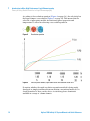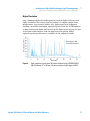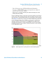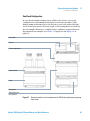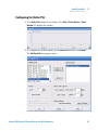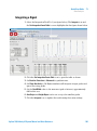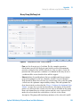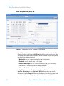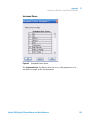
Download Ultra Start 1250 SERIES Technical data

Agilent 1290 Infinity
LC System
System Manual and
Quick Reference
Agilent Technologies
Notices
© Agilent Technologies, Inc. 2009-2011,
2012
No part of this manual may be reproduced
in any form or by any means (including electronic storage and retrieval or translation
into a foreign language) without prior agreement and written consent from Agilent
Technologies, Inc. as governed by United
States and international copyright laws.
Manual Part Number
G4220-90301
Edition
05/2012
Printed in Germany
Agilent Technologies
Hewlett-Packard-Strasse 8
76337 Waldbronn
This product may be used as a component of an in vitro diagnostic system if the system is registered with
the appropriate authorities and complies with the relevant regulations.
Otherwise, it is intended only for general laboratory use.
Warranty
The material contained in this document is provided “as is,” and is subject to being changed, without notice,
in future editions. Further, to the maximum extent permitted by applicable
law, Agilent disclaims all warranties,
either express or implied, with regard
to this manual and any information
contained herein, including but not
limited to the implied warranties of
merchantability and fitness for a particular purpose. Agilent shall not be
liable for errors or for incidental or
consequential damages in connection
with the furnishing, use, or performance of this document or of any
information contained herein. Should
Agilent and the user have a separate
written agreement with warranty
terms covering the material in this
document that conflict with these
terms, the warranty terms in the separate agreement shall control.
receive no greater than Restricted Rights as
defined in FAR 52.227-19(c)(1-2) (June
1987). U.S. Government users will receive
no greater than Limited Rights as defined in
FAR 52.227-14 (June 1987) or DFAR
252.227-7015 (b)(2) (November 1995), as
applicable in any technical data.
Safety Notices
CAUTION
A CAUTION notice denotes a
hazard. It calls attention to an
operating procedure, practice, or
the like that, if not correctly performed or adhered to, could
result in damage to the product
or loss of important data. Do not
proceed beyond a CAUTION
notice until the indicated conditions are fully understood and
met.
Technology Licenses
The hardware and/or software described in
this document are furnished under a license
and may be used or copied only in accordance with the terms of such license.
Restricted Rights Legend
If software is for use in the performance of a
U.S. Government prime contract or subcontract, Software is delivered and licensed as
“Commercial computer software” as
defined in DFAR 252.227-7014 (June 1995),
or as a “commercial item” as defined in FAR
2.101(a) or as “Restricted computer software” as defined in FAR 52.227-19 (June
1987) or any equivalent agency regulation
or contract clause. Use, duplication or disclosure of Software is subject to Agilent
Technologies’ standard commercial license
terms, and non-DOD Departments and
Agencies of the U.S. Government will
WA R N I N G
A WARNING notice denotes a
hazard. It calls attention to an
operating procedure, practice,
or the like that, if not correctly
performed or adhered to, could
result in personal injury or
death. Do not proceed beyond a
WARNING notice until the indicated conditions are fully understood and met.
Agilent 1290 Infinity LC System Manual and Quick Reference
In This Guide...
In This Guide...
This manual covers the Agilent 1290 Infinity LC System.
1 Introduction to Ultra-High Performance Liquid Chromatography
This chapter gives an introduction to the Agilent 1290 Infinity LC System and
the underlying concepts.
2 The Agilent 1290 Infinity LC System - Product Description
This chapter discusses the features of the 1290 Infinity LC System.
3 Optimization of the Agilent 1290 Infinity LC System
This chapter considers how to apply the theory and use the features of the LC
system to develop optimized separations.
4 System Setup and Installation
This chapter includes information on software installation, stack
configurations and preparing the system for operation.
5 Quick Start Guide
This chapter provides information on data acquisition and data analysis with
the 1290 Infinity LC System.
6 Appendix
This chapter provides additional information on safety, legal and web and
about setting up a method.
Agilent 1290 Infinity LC System Manual and Quick Reference
3
Contents
Contents
1 Introduction to Ultra-High Performance Liquid Chromatography
7
Theory of Using Smaller Particles in Liquid Chromatography 8
Benefits of Columns Packed With Sub-2-micron Particles 14
Frictional Heating 18
2 The Agilent 1290 Infinity LC System - Product Description
New Features of the Agilent 1290 Infinity LC System
System Components 25
22
3 Optimization of the Agilent 1290 Infinity LC System
39
21
Delay Volume and Extra-Column Volume 40
How to Configure the Optimum Delay Volume 42
How to Achieve Higher Injection Volumes 51
How to Achieve High Throughput 53
How to Achieve Higher Resolution 56
How to Achieve Higher Sensitivity 59
How to Achieve Lowest Carry Over 66
How to Prevent Column Blockages 68
4 System Setup and Installation
71
Installing Software 72
Installing the Module 73
5 Quick Start Guide
89
About the Quick Start Guide 90
Preparing the system 91
Data Acquisition in Method and Run Control View
Data Analysis 103
4
96
Agilent 1290 Infinity LC System Manual and Quick Reference
Contents
6 Appendix
109
Safety Information 110
Solvent Information 113
Agilent Technologies on Internet 114
Setting Up a Method using Edit Entire Method
Agilent 1290 Infinity LC System Manual and Quick Reference
115
5
Contents
6
Agilent 1290 Infinity LC System Manual and Quick Reference
Agilent 1290 Infinity LC System Manual and Quick Reference
1
Introduction to Ultra-High Performance
Liquid Chromatography
Theory of Using Smaller Particles in Liquid Chromatography
Benefits of Columns Packed With Sub-2-micron Particles
Frictional Heating
8
14
18
This chapter gives an introduction to the Agilent 1290 Infinity LC System and
the underlying concepts.
Agilent Technologies
7
1
Introduction to Ultra-High Performance Liquid Chromatography
Theory of Using Smaller Particles in Liquid Chromatography
Theory of Using Smaller Particles in Liquid Chromatography
Introduction
In 2003, Agilent introduced the first commercially available porous silica
columns with 1.8 µm particles. These were the first in a class of columns
which has become known as ‘sub-two micron’ or STM columns. For use with
the Agilent 1200 Series Rapid Resolution LC system, launched in 2006, these
packing materials were introduced in ZORBAX RRHT columns capable of
withstanding 600 bar pressure. In 2009 the range was extended to include
RRHD columns capable of routine use at 1200 bar pressure to support the
introduction of the Agilent 1290 Infinity LC System with its extensive
operating power range up to 1200 bar pressure and 5 ml/min flow rate.
These sub-two micron (1.8 µm) particle size columns can be used in pursuit of
two main objectives:
1 Faster Chromatography
Short columns with sub-two-micron particles offer the opportunity to
dramatically reduce analysis time by increasing the flow rate without losing
separation performance.
2 Higher Resolution
Long columns with sub-two-micron particles provide higher efficiency and
therefore higher resolution, required for the separation of complex samples.
Lower dispersion also means less dilution of the analyte peaks and
consequent sensitivity gains, particularly for LC/MS.
The pressure needed to drive solvent through a column containing STM
particles rises rapidly as flow rate is increased for faster separations and very
rapidly as the length of the column increases for more resolution. Thus the
acceptance of STM columns has been synonymous with the development of
UHPLC systems – that is HPLC systems that offer higher pressures than the
400 bar norm that was extant since the early days of HPLC. Ultra-High
Performance (or Ultra-High Pressure) LC systems also offer low delay volumes
and the fast data collection required for narrow peaks from fast or high
resolution chromatography. The Agilent 1290 Infinity LC is a landmark in
UHPLC as it is the first system that can completely cover and extend upon all
the disparate performance ranges of UHPLCs pre-existing on the market.
8
Agilent 1290 Infinity LC System Manual and Quick Reference
Introduction to Ultra-High Performance Liquid Chromatography
Theory of Using Smaller Particles in Liquid Chromatography
1
The Theory
I]ZdgZi^XVaEaViZ=Z^\]i=
Separation efficiency in HPLC can be described by the van Deemter equation
(Figure 1 on page 9). This results from the plate-height model used to measure
the dispersion of analytes as they move down the column. H is the Height
Equivalent to a Theoretical Plate (sometimes HETP), dp is the particle size of
the column packing material, u0 is the linear velocity of the mobile phase and
A, B and C are constants related to the different dispersive forces. The A term
relates to eddy diffusion or multiple flow paths through the column; B relates
to molecular diffusion along the column axis (longitudinal); C relates to mass
transfer of the analyte between the mobile and stationary phases. The
separation is at its most efficient when H is at a minimum. The effect of each
individual term and the combined equation are shown in Figure 1 on page 9
where the plate height is plotted against the linear flow rate through the
column. This type of plot is known as a Van Deemter Curve and is used to
determine the optimum flow rate (minimum point of the curve) for best
efficiency of separation for a column.
aVg\ZeVgi^XaZ
hbVaaeVgi^XaZ
GZhjai^c\KVc"9ZZbiZgXjgkZ
GZh^hiVcXZidBVhhIgVch[Zg
Bjai^eVi]IZgb!
:YYn9^[[jh^dc
Adc\^ijY^cVaY^[[jh^dc
Figure 1
A^cZVg[adlj
A hypothetical Van Deemter curve
Agilent 1290 Infinity LC System Manual and Quick Reference
9
1
Introduction to Ultra-High Performance Liquid Chromatography
Theory of Using Smaller Particles in Liquid Chromatography
The van Deemter plots in Figure 2 on page 10 show that reducing particle size
increases efficiency. Switching from commonly used 3.5 µm and 5.0 µm
particle sizes to 1.8 µm particles offers significant performance improvements.
The 1.8 µm particles give two to three times lower plate height values and
proportionately higher efficiencies. This allows a shorter column to be used
without sacrificing resolution and hence the analysis time is also reduced by a
factor of two to three. The increased efficiency is derived to a large extent
from the reduction in multiple flow paths as a result of the smaller particles this leads to a smaller A term (eddy diffusion). In addition, smaller particles
mean shorter mass transfer times, reducing the C term, and it can be seen that
the overall effect is a much reduced loss of efficiency as the flow rate increases
(the slope of the line is reduced). This means that the separation on smaller
particles can be further accelerated by increasing the flow rates without
significantly reducing efficiency.
%#%%)*
%#%%)%
=:IEXb$eaViZ
%#%%(*
%#%%(%
%#%%'*
*#%¥b
%#%%'%
%#%%&*
(#*¥b
%#%%&%
&#-¥b
%#%%%*
%#%%%%
*#%ba$b^c
'ba$b^c
"%#%%%*
%#%
%#'
%#)
%#+
%#-
&#%
&#'
&#)
&#+
>ciZghi^i^Vaa^cZVgkZadX^in¥"Xb$hZX
Z
Figure 2
10
Van Deemter curve for different particle sizes
Agilent 1290 Infinity LC System Manual and Quick Reference
Introduction to Ultra-High Performance Liquid Chromatography
Theory of Using Smaller Particles in Liquid Chromatography
1
A chromatographic separation can be optimized based on physical parameters
of the HPLC column such as particle size, pore size, morphology of the
particles, the length and diameter of the column, the solvent velocity, and the
temperature. In addition, the thermodynamics of a separation can be
considered and the properties of the solute and the stationary and mobile
phases (percentage of organic solvent, ion strength, and pH) can be
manipulated to achieve the shortest possible retention and highest selectivity.
DEI>B>O:
@>C:I>8H
d[H:E6G6I>DC
Hadl6Y"dg9Zhdgei^dc
DEI>B>O:
I=:GBD9NC6B>8H
d[H:E6G6I>DC
Cdc"a^cZVg^hdi]Zgbh
8]Zb^XVa:fj^a^Wgjbe=
EgZhhjgZ
E=NH>8H
8=:B>HIGN
EVgi^XaZH^oZ!Edgdh^in!
8dajbc9^bZch^dch!
;adlKZadX^in!IZbeZgVijgZ
HiVi^dcVgnVcYBdW^aZ
E]VhZEgdeZgi^Zh!HdajiZ
EgdeZgi^Zh!IZbeZgVijgZ
Figure 3
Selecting optimal conditions for HPLC
Resolution can be described as a function of three parameters:
• column efficiency or theoretical plates (N),
• selectivity (),
• retention factor (k).
Agilent 1290 Infinity LC System Manual and Quick Reference
11
1
Introduction to Ultra-High Performance Liquid Chromatography
Theory of Using Smaller Particles in Liquid Chromatography
According to the resolution equation ( Figure 4 on page 12 ), the selectivity has
the biggest impact on resolution (Figure 5 on page 12). This means that the
selection of appropriate mobile and stationary phase properties and
temperature is critical in achieving a successful separation.
Figure 4
Resolution equation
Figure 5
Effect of plate number, separation factor and retention factor on R
No matter whether the rapid resolution separation method is being newly
developed or simply transferred from an existing conventional method, it is
clearly beneficial to have a wide choice of stationary phase chemistries
available in a range of column formats.
12
Agilent 1290 Infinity LC System Manual and Quick Reference
Introduction to Ultra-High Performance Liquid Chromatography
Theory of Using Smaller Particles in Liquid Chromatography
1
Agilent already offered more than 140 ZORBAX 1.8 µm Rapid Resolution High
Throughput (RRHT) columns (14 selectivity choices; 15 to 150 mm long; 2.1,
3.0 and 4.6 mm internal diameters) and with the launch of the Agilent 1290
Infinity LC the STM range is extended to include the Rapid Resolution High
Definition (RRHD) 1200 bar columns. This enables the optimum stationary
phase to be selected so that the selectivity is maximized. The resolution, flow
rate and analysis time can be optimized by selecting the appropriate column
length and diameter and operation with longer STM columns has become more
accessible than ever before.
Many laboratories perform an extensive screening process to select the best
combination of stationary phase, mobile phase and temperature for their
separations. Agilent offers Method Development Solutions on both the 1200
Series and 1290 Infinity LC systems. These offer complete automation of this
time consuming selection process – making method development and method
transfer an easier and more reliable task.
ZORBAX 1.8 µm RRHD and RRHT columns use the same chemistry as
ZORBAX columns with 3.5 and 5 µm particles. As a result, for any particular
ZORBAX phase, the 5.0, 3.5 and 1.8 µm particles provide identical selectivity,
which allows easy, fast and secure bidirectional method transfer between
conventional LC, UHPLC and preparative LC.
Agilent 1290 Infinity LC System Manual and Quick Reference
13
1
Introduction to Ultra-High Performance Liquid Chromatography
Benefits of Columns Packed With Sub-2-micron Particles
Benefits of Columns Packed With Sub-2-micron Particles
Faster Chromatography
There are several advantages of having shorter run times. High Throughput
labs now have higher capacity and can analyze more samples in less time.
More samples in less time also means lower costs. For example, by reducing
the analysis time from 20 min per sample to 5 min, the cost for 700 samples is
reduced by 79 % (Table 1 on page 14).
Table 1
Time and cost savings over 700 runs
Cycle time
20 min cycle time
5 min cycle time
Runs
700
700
Approx. costs/analysis1
$ 10.58
$ 2.24
Approx. cost/700runs1
$ 7400
$ 1570
Cost savings
-
$ 5830
Time2
10 days
2.5 days
1
solvents = $ 27/l, disposal = $ 2/l, labor = $ 30/h
2
24 hours/day
The Agilent cost savings calculator provides an easy way to calculate the cost
savings by switching from conventional HPLC to UHPLC using 1.8 µm particle
size columns. This calculator is available on the Agilent Technologies web site
along with a method translator calculator – www.chem.agilent.com. The
results are presented graphically and in tabular form.
Shorter run times also deliver faster answers. This is important in process
control and rapid release testing. Instead of waiting hours to release a single
batch of a drug, all the system suitability, calibration and sample analysis can
now be done in less than an hour. Rapid answers are also important for
synthetic chemists using open access LC/MS systems for compound
confirmation and reaction control. Shorter run times can also accelerate the
method development process significantly.
14
Agilent 1290 Infinity LC System Manual and Quick Reference
Introduction to Ultra-High Performance Liquid Chromatography
Benefits of Columns Packed With Sub-2-micron Particles
Figure 6
1
Cost savings calculator
Agilent 1290 Infinity LC System Manual and Quick Reference
15
1
Introduction to Ultra-High Performance Liquid Chromatography
Benefits of Columns Packed With Sub-2-micron Particles
8dajbc
AZc\i]
bb
8dajbc
:[[^X^ZcXn
C*¥b
8dajbc
:[[^X^ZcXn
C(#*¥b
8dajbc
:[[^X^ZcXn
C&#-¥b
&*%
&'!*%%
'&!%%%
(*!%%%
&%%
-!*%%
&)!%%%
'(!'*%
,*
+%%%
&%!*%%
&,!*%%
,!%%%
&'!%%%
6cVanh^h
I^bZ
GZYjXi^dc
:[[^X^ZcXn
6cVanh^h
C
I^bZ
"((
"*%
EgZhhjgZ
*%
)!'%%
EZV`
"+,
KdajbZ
(%
C#6#
)!'%%
+!*%%
HdakZci
"-%
JhV\Z
&*
C#6#
Figure 7
16
'!&%%
'!*%%
".%
Relation between particle size, efficiency and analysis time
Agilent 1290 Infinity LC System Manual and Quick Reference
Introduction to Ultra-High Performance Liquid Chromatography
Benefits of Columns Packed With Sub-2-micron Particles
1
Higher Resolution
6WhdgWVcXZPb6JR
Long columns packed with smaller particles result in higher efficiency and
higher resolution. This is important for analysis of complex samples from
metabolomics or proteomics studies. Also, applications such as impurity
profiling can benefit from higher separation power. Even the LC/MS analysis
of drugs in biological fluids can benefit from the higher peak capacity, because
of the reduced interference from ion suppression. In general, higher
separation power provides more confidence in the analytical results.
EZV`XVeVX^in2+.)
A8l^i]<8gZhdaji^dc
I^bZPb^cR
Figure 8
Peak capacities of more than 700 can be achieved using a ZORBAX RRHT
SB-C18 column (2.1 x 150 mm, 1.8 µm) to analyze a tryptic digest of BSA
Agilent 1290 Infinity LC System Manual and Quick Reference
17
1
Introduction to Ultra-High Performance Liquid Chromatography
Frictional Heating
Frictional Heating
Forcing mobile phase through the column at higher pressure and higher flow
rates generates heat. The resulting temperature gradients (radial and
longitudinal) can have an impact on the column efficiency.
where F is the flow rate and p is the pressure.
Powerful column thermostatting (for example, using a water bath) generates a
strong radial temperature gradient, which leads to significant loss in column
efficiency. Still-air column thermostatting reduces the radial temperature
gradient and therefore reduces the efficiency losses, but a higher column
outlet temperature has to be accepted. The raised temperature may have an
effect on selectivity. At lower back-pressure, performance losses due to
frictional heat are minimized so that 4.6 or 3 mm inner diameter sub-2-micron
columns still deliver superior efficiencies compared with the respective
2.1 mm inner diameter columns.
An example of a gradient method transfer to a 2.1 mm i.d. STM column in
which the separation has been speeded up is shown in Figure 9 on page 19.
The initial run on the 2.1 mm column was at a flow rate of 0.22 ml/min
generating 380 bar pressure at a temperature setting of 37 °C with all peaks
separated in 12.5 min (chromatogram not shown). The flow was increased to
0.66 ml/min and the gradient times adjusted downwards by a factor of three
generating 1020 bar pressure with all peaks eluted in 4.2 min (Figure 9 on
page 19 above). This should give the same separation but a loss of resolution
can be seen between peaks 7 and 8 and between 5 and the main peak and this
is due to heating in the column changing the selectivity for these compounds.
It was found that running the column thermostat at 5 °C lower was sufficient
to offset the heating effect inside the column and restore the separation
(Figure 9 on page 19 below). The pressure increased to 1070 bar which also
indicates that the in-column temperature was lower.
18
Agilent 1290 Infinity LC System Manual and Quick Reference
Introduction to Ultra-High Performance Liquid Chromatography
Frictional Heating
Figure 9
1
Influence of frictional heat generation on selectivity and effect of lowering
column temperature
In summary, the use of sub-two-micron packing material offers benefits of
increased efficiency, higher resolution and faster separations. The Agilent
1290 Infinity LC System and RRHD columns increase the separation space
available and enable more of these benefits to be accessed. The features of the
1290 Infinity LC are discussed in “The Agilent 1290 Infinity LC System Product Description” on page 21 and “Optimization of the Agilent 1290
Infinity LC System” on page 39considers how to apply the theory and use
these features to develop optimized separations.
Agilent 1290 Infinity LC System Manual and Quick Reference
19
1
20
Introduction to Ultra-High Performance Liquid Chromatography
Frictional Heating
Agilent 1290 Infinity LC System Manual and Quick Reference
Agilent 1290 Infinity LC System Manual and Quick Reference
2
The Agilent 1290 Infinity LC System Product Description
New Features of the Agilent 1290 Infinity LC System
System Components
22
25
This chapter discusses the features of the 1290 Infinity LC System.
Agilent Technologies
21
2
The Agilent 1290 Infinity LC System - Product Description
New Features of the Agilent 1290 Infinity LC System
New Features of the Agilent 1290 Infinity LC System
The Agilent 1290 Infinity LC System is designed to offer the greatest flexibility
for performing analytical liquid chromatography using all types of current and
emergent column technologies. The 1290 Infinity LC has the widest range of
operating parameters so that it can replicate method settings transferred in
from any pre-existing analytical HPLC or UHPLC system available from any
vendor. The Agilent 1290 Infinity LC System offers some radical new design
concepts to achieve this objective and yet clearly shows the pedigree of
well-engineered reliability that has made Agilent HPLC systems the most
successful HPLC line available.
This system offers:
• Flow rates from 0.05 ml/min to 5 ml/min for conventional or fast
chromatography with all analytical column diameters from 1 to 5 mm
internal diameter and all types of column packing material.
• Pressure range up to 1200 bar (>17400 psi) allows for fast chromatography
on short columns, high resolution on long columns using sub-two micron
packing material and a wider choice of mobile phase viscosity.
• Ultra-low delay volumes for the fastest gradients with mass spectrometric
detection or ultraviolet/visible light detection.
• Ability to operate any method transferred from another analytical HPLC or
UHPLC system.
• Sophisticated pump control to deliver very low chromatographic noise and
very low acoustic noise for better results and better working environment.
• Degasser and automatic purge valve integrated into pump module.
• Variable volume autosampler with reduced delay volume, reduced
carryover and the option to operate as a fixed loop autosampler.
• New Flexible Cube module to add functionality to the autosampler such as
back-flushing the needle seat and fixed loop operation.
• Thermostatted Column Compartment with enhanced usability and
integrated valve solutions with a pressure range up to 1200 bar (17400 psi).
• Diode-array detector with greatly enhanced sensitivity and baseline
stability using cartridge cell system with optofluidic waveguides.
22
Agilent 1290 Infinity LC System Manual and Quick Reference
The Agilent 1290 Infinity LC System - Product Description
New Features of the Agilent 1290 Infinity LC System
2
• Data collection rates up to 160 Hz with full spectral information.
• New range of ZORBAX RRHD sub-two micron particle size columns for
operation at pressures up to 1200 bar.
• Blend Assist for automatic buffering and additive blending in the 1290
Infinity Quaternary Pump.
The most significant advance is the range of pressures and flow rates that the
system can use. This operating envelope can be described as the power range
(flow x pressure) of the instrument and is most easily understood in graphical
form (Figure 10 on page 23). As can be seen from the diagram the power range
for the 1290 Infinity pump allows 1200 bar operation up to 2 ml/min flow,
reducing to 800 bar as flow increases to 5 ml/min. This encompasses the
operating range envelopes of all pre-existing UHPLC systems on the market
and makes possible the direct transfer of methods from any of these systems
to the 1290 Infinity system.
&'.%>c[^c^in
KZcYdg6
KZcYdg9
KZcYdg7
6\^aZciGGA8
KZcYdg8
HiVcYVgYA8
Figure 10
Power range of UHPLC systems (pressure x flow rate operating space)
Agilent 1290 Infinity LC System Manual and Quick Reference
23
2
The Agilent 1290 Infinity LC System - Product Description
New Features of the Agilent 1290 Infinity LC System
The pressure range offers the ability to work with the latest sub-two micron
particles in long columns for high resolution and short columns for fast
separation at increased flow rates. The flow rate range allows not only
traditional methods to be used but also superficially porous (or pellicular)
packing materials (for example, Poroshell) at high flow rates. These types of
packing have recently gained new interest as an alternative approach to STM
materials for high efficiency separations. The flow rate range allows the most
suitable diameter column to be chosen for the separation whether it is 2 mm
for low flow applications such as required by some MS systems or up to 5 mm
id (typically 4.6 mm) for more traditional LC or increased loadability. The flow
rate range also supports the latest research findings that show the benefit of
using maximum flow rates to increase efficiency in gradient separations.
(Refer to Petersson et al., J.Sep.Sci, 31, 2346-2357, 2008, Maximizing peak
capacity and separation speed in liquid chromatography).
The new diode-array detector offers new levels of sensitivity combined with
outstanding baseline characteristics and ease of use due to an innovative cell
design.
The autosampler offers the well-established Agilent flow-through design for
variable volume injection with low carryover upgraded for higher pressure,
lower volume applications. A completely new module, the Flexible Cube, can
be added on to the autosampler to offer fixed loop injection for the absolute
lowest delay volume and other performance enhancements such as needle seat
backflushing.
24
Agilent 1290 Infinity LC System Manual and Quick Reference
2
The Agilent 1290 Infinity LC System - Product Description
System Components
System Components
The Agilent 1290 Infinity Binary Pump
The Agilent 1290 Infinity Binary Pump contains new technology to overcome
the problems of pumping LC solvents at ultra-high pressure and high flow
rates: heavy duty drive motors on the pistons; new material for the pistons
themselves not only to withstand the workload but also to actively transfer
heat from the seals; microfluidic heat exchangers and the Jet Weaver, a
microfluidic mixing device. The pump can deliver flow in the range of 0.05 –
5 mL/min at pressures up to 1200 bar.
The Agilent 1290 Infinity Binary Pump module contains two identical high
pressure (1200 bar) pumps; a two-channel solvent degasser and four-channel
inlet solvent selection valve, automatic purge valve and low-volume mixing
device, the Jet Weaver, integrated into a single housing. The degasser increases
flow stability, especially at low flow rates, and detector sensitivity.
Figure 11
The Agilent 1290 Infinity Binary Pump
Agilent 1290 Infinity LC System Manual and Quick Reference
25
2
The Agilent 1290 Infinity LC System - Product Description
System Components
IdVjidhVbeaZg
;gdbhdakZcigZhZgkd^gh
HdakZci
hl^iX]^c\
kVakZ
B^mZg
9Z\VhhZg
Eg^bVgn
ejbe]ZVY
EgZhhjgZ
hZchdg
Eg^bVgn
ejbe]ZVY
8]VccZa6
Figure 12
HZXdcYVgn 8]VccZa7
ejbe]ZVY
HZXdcYVgn
ejbe]ZVY
IdlVhiZ
Parts identification and schematic of the 1290 Infinity Binary Pump
Each pump head is a dual piston in-series design utilizing novel firmware
control and novel piston material, silicon carbide, which efficiently removes
heat from the pump. The capillary joining the primary piston to the secondary
piston has an integrated heat exchanger to remove the heat created at high
pressure and flow. Each pump head has one passive inlet valve and one
passive outlet valve on the primary piston chamber. Each piston is
independently and precisely driven by a motor with 65000 steps giving 300
picolitres displacement per step.
The movement of the pistons is under intelligent control with a feedback loop
to ensure that this active damping of pressure pulsation results in a ripple-free
flow. The piston drive tunes itself for the compressibility characteristics of the
solvent and the hydraulic characteristics of the system to maintain the
ripple-free state. This in conjunction with the smooth-motion control, which
reduces pressure pulsation caused by the movement of the piston, and the
low-volume efficient mixing ensure that pump noise on UV traces is the lowest
possible. A dedicated microprocessor in the pump takes care of the smooth
motion control and optimization of the pistons’ motion for real-time
optimization based on the static and dynamic parameters. In addition to the
26
Agilent 1290 Infinity LC System Manual and Quick Reference
2
The Agilent 1290 Infinity LC System - Product Description
System Components
chromatographic performance these features makes the pump very quiet in
operation.
When concentrated buffer solutions are used as mobile phase, the active seal
wash option is available for use to extend the life of the pump seals.
A solvent selection valve allows binary mixtures (isocratic or gradient) to be
formed from one of two solvents per channel. Binary gradients are created at
the purge valve by high-pressure mixing of solvents from pump A and pump B.
The purge valve allows the flow to be switched under software control to
waste for purging new solvents through the pump head. A sensor is connected
to the purge valve to monitor the system pressure.
Figure 13
The Jet Weaver mixer
Agilent 1290 Infinity LC System Manual and Quick Reference
27
2
The Agilent 1290 Infinity LC System - Product Description
System Components
The flow path of the pump has been optimized for minimal delay of gradients
and incorporates an innovative mixing system using microfluidics technology.
The mixing device, known as the Jet Weaver, employs a network of multi-layer
microfluidic channels (120 µm x 120 µm) to unsure the flow is thoroughly
mixed. The Jet Weaver has two standard volumes: 35 µl for normal UV
detection applications and 100 µl for demanding situations such as the use of
TFA in UV detection. For uncompromisingly low baseline noise in these
demanding applications, a 380 µL Jet Weaver is also available. For MS
detection it is often possible to work without the Jet Weaver and attain
sufficient mixing using only the base 10 µl volume of the pump flow-path.
Typical applications are high throughput methods with fast gradients on high
resolution 2.1 mm columns.
The 1290 Infinity Binary pump comes ready for additional valve rails to be
mounted on the right or left side of the pump. On these valve rails up to two
additional 12-fold solvent selection valves can be attached. This allows a
maximum of 26 solvents for binary gradients for analytical method
development. A special “cluster driver” is available that makes the external
solvent selection valves part of the pump user interface and allows very
user-friendly and easy selection of the solvents by their names.
28
Agilent 1290 Infinity LC System Manual and Quick Reference
The Agilent 1290 Infinity LC System - Product Description
System Components
2
The 1290 Infinity Quaternary Pump
In contrast, the 1290 Infinity Quaternary Pump is equipped with only one
pump head and an additional multi-channel gradient valve (MCGV) to portion
the eluents according to the programmed gradient. According to this low
pressure mixing principle, the solvents meet in the Inlet Weaver and are
therefore already mixed before and in the pump head.
The pump head is the same as that in the 1290 Infininty Binary Pump and
therefore has the same performance values and technical details. It can also be
equipped with an active seal wash to extend the lifetime of the pump seals,
when using concentrated buffer solutions.
A pressure sensor monitors the pressure during the analysis before the
solvents enter the multi-purpose valve, a 4-channel stream selector, which
allows different functionalities shown in the figures below. The multi-purpose
valve is equipped with an in-line filter, which will always be used during an
analysis, an optional 380 µL Jet Weaver mixer, which ensures the best possible
mixing of solvents and can be easily installed, an optional restriction capillary
and a connection to the waste system.
Agilent 1290 Infinity LC System Manual and Quick Reference
29
2
The Agilent 1290 Infinity LC System - Product Description
System Components
Table 2
Valve functionalities
Pump
Pump
Agilent
Jet Weaver
Agilent
Jet Weaver
Sampler
Sampler
Waste
Waste
Filter
Figure 14
Filter
Standard application
Figure 15
Extra-mixing volume setup
Pump
Pump
Agilent
Jet Weaver
Agilent
Jet Weaver
Sampler
Sampler
Waste
Waste
Filter
Filter
Figure 16
30
Automatic purge function
Figure 17
Backflushing the in-line filter
Agilent 1290 Infinity LC System Manual and Quick Reference
The Agilent 1290 Infinity LC System - Product Description
System Components
2
The standard application (1) is used for the majority of analysis, while the
extra-mixing volume setup (2) is applied for any kind of baseline-criticial
application where the mixing performance and the dependant UV-baseline can
be significantly enhanced by the use of the Agilent Jet Weaver mixer. An
automatic purge function (3) is installed, as well as the possibility of
backflushing the in-line filter (4). This enables you to clean the filter and
extend its lifetime.
Agilent 1290 Infinity LC System Manual and Quick Reference
31
2
The Agilent 1290 Infinity LC System - Product Description
System Components
The Agilent 1290 Infinity Autosampler
The Agilent 1290 Infinity Autosampler offers the well-established Agilent
flow-through design with variable volume injection and takes it to new levels
of performance. New inert materials in the metering device seal and needle
seat help to achieve extremely low carryover. The reduced hydraulic volume of
the flow path is suited to faster gradients and the ability to use overlapped
injections and automatic delay volume reduction (ADVR) contribute to faster
cycle times and even faster gradient delivery to the column. The system draws
exactly the set volume of sample solution without waste and achieves high
reproducibility across the range from sub-microlitre to maximum injection
volume of 40 µl. The standard installed injection capillary allows injections to
20 µl.
&#KVakZ^cbV^ceVhh![adli]gdj\]
'#KVakZ^cWneVhh!YgVl^c\hVbeaZ
(#KVakZ^cWneVhh!lVh]^c\cZZYaZ
)#KVakZ^cbV^ceVhh!hVbeaZ^c_ZXiZY
Figure 18
32
Schematic of injection steps in 1290 Infinity Autosampler
Agilent 1290 Infinity LC System Manual and Quick Reference
The Agilent 1290 Infinity LC System - Product Description
System Components
2
A totally new optional add-on module, the Flexible Cube, works seamlessly
with the autosampler to provide additional capabilities. With the addition of
the new Flexible Cube module, which comprises a 500 µl syringe pump, one
low pressure valve and two high pressure switching valves further options
become possible. For instance, the flow-through injection system can be
replaced by a fixed injection loop using the syringe pump and valving of the
Flexible Cube to fill the sample loop. The advantage of this configuration is
that it eliminates the delay volume from the autosampler and so may be
preferred in some fast-gradient high-throughput situations. The trade-off is
that the flexibility of variable volume injection is turned off and some sample
is wasted in flushing the loop. Other tasks such as automatically back-flushing
the injection needle seat after injection are possible with the Flexible Cube
giving further confidence that carryover of difficult compounds or blockages
caused by dirty samples can be routinely avoided.
The autosampler sample rack has 10 fixed positions for 2 ml vials and two
removable trays, which may or may not be identical, selected from:
• Tray for 2 ml vials with 54 positions
• Microtitre plate with 96 well positions (various heights configurable)
• Microtitre plate with 384 well positions (various heights configurable)
If required the autosampler can be thermostatted from 4 °C to 40 °C by the
addition of the autosampler temperature control module.
Agilent 1290 Infinity LC System Manual and Quick Reference
33
2
The Agilent 1290 Infinity LC System - Product Description
System Components
The Agilent 1290 Infinity Thermostatted Column Compartment
The Agilent 1290 Infinity Thermostatted Column Compartment (TCC) controls
the temperature between 10 °C below ambient and up to 100 °C at 2.5 ml/min
and 80 °C at up to 5 ml/min, respectively. The temperature stability
specification is ± 0.05 °C and the accuracy specification ±0.5 °C (with
calibration)1. This is achieved by a combination of conduction from contact
with the thermostat vanes, still-air temperature in the column environment
and most importantly by pre-heating (or cooling) the mobile phase by passing
it through a heat exchanger before entering the column. There are two
independent temperature zones in each TCC which can work together for long
columns up to 300 mm length or work at different temperatures for short
columns of 100 mm length or less.
The module comes with a 1.6 µl low dispersion heat exchanger and each valve
kit contains additional low dispersion heat exchangers for each column. The
low dispersion heat exchangers, up to 4, can be mounted flexibly inside the
TCC. For conventional HPLC operation, 3 µl and 6 µl built-in heat exchangers
are also available.
Each TCC can accommodate one internal valve drive to facilitate valve
switching applications from simple switching between two columns to
automatic column regeneration, sample preparation or column back-flushing.
Each valve head comes as a complete kit containing all required capillaries,
additional low dispersion heat exchangers and other parts.
The switching valves have exceptional ease-of-use and flexibility when making
connections to the valve: When pressed, the drive unit of the Quick Change
Valve slides forward for easy access (see Figure 19 on page 35 left). Alternative
valve heads can be interchanged by the user on the drive mechanism for
different applications (see Figure 19 on page 35 right). Note the RFID tag on
top of valve head.
1
34
All specifications are valid for distilled water at ambient temperature of 25 °C, setpoint at 40 °C
and a flow range from 0.2 to 5 ml/min.
Agilent 1290 Infinity LC System Manual and Quick Reference
2
The Agilent 1290 Infinity LC System - Product Description
System Components
Figure 19
Quick change valve in TCC
Up to three TCC can be “clustered” to allow advanced applications such as
switching between eight columns for automated method development or to
make additional columns available for different applications. Thus, the column
to be used becomes a simple method parameter. This requires two 8 position/9
port valve heads, one each in two of the TCCs. Clustered TCC are represented
by the software as one unit with one interface for ease of operation.
Further improvements compared to earlier designs include better thermal
insulation, better capillary guides and a “door open” sensor so that methods
can define that the door must be closed – especially useful for low or
high-temperature methods.
Agilent 1290 Infinity LC System Manual and Quick Reference
35
2
The Agilent 1290 Infinity LC System - Product Description
System Components
The 1290 Infinity Diode-Array Detector
The 1290 Infinity Diode-Array Detector is a new optical design using a
cartridge cell with optofluidic waveguide technology offering high sensitivity
with low dispersion, a wide linear range and a very stable baseline for
standard or ultra-fast LC applications. The Agilent Max-Light cartridge cell
dramatically increases the light transmission by utilizing the principle of total
internal reflection along a non-coated fused silica capillary, achieving a new
level of sensitivity without sacrificing resolution through cell volume
dispersion effects. This design minimizes baseline perturbations caused by
refractive index or thermal effects and results in more reliable integration of
peak areas.
B^ggdg
<gVi^c\
Deid[aj^Y^XlVkZ\j^YZ
9ZjiZg^jbaVbe
BVm"a^\]iXVgig^Y\ZXZaa
Egd\gVbbVWaZha^i
&%')ZaZbZciY^dYZ"VggVn
Figure 20
36
The light path through the 1290 Infinity Diode-Array Detector
Agilent 1290 Infinity LC System Manual and Quick Reference
The Agilent 1290 Infinity LC System - Product Description
System Components
2
The module also incorporates electronic temperature control to further
enhance the resistance to ambient temperature effects. Although the hydraulic
volume of the Max-Light cartridge cell is very small, the path length is a
standard 10 mm. However, for even higher sensitivity the alternative Agilent
Max-Light high sensitivity cell is available with a path length of 60 mm. Cells
are easily exchanged by sliding them in or out of the cell holder and they are
auto-aligned in the optical bench. The DAD light source is a deuterium lamp
and the operating wavelength range covered is 190 to 640 nm. This is detected
by a diode-array comprising 1024 diodes. The entrance to the spectrograph is
through a programmable optical slit which can give spectral resolution from 1
to 8 nm. This is generally operated in the middle of the range but for
optimization can be closed down to 1nm for high spectral resolution (rarely
required in liquid phase UV spectra) or opened up to 8 nm for maximum light
transmission and minimum noise in the signal.
The chromatographic signals are extracted from the diode-array data within
the firmware of the module. Up to 8 individual signals can be defined, each
comprising a signal wavelength, a diode-bunching bandwidth and, if required,
a reference wavelength and bandwidth. Signals can be output at up to 160 Hz
(160 data points/second) for accurate recording of the fastest (narrowest)
chromatographic peaks. At the same time the module can also output
full-range spectra to the data system at the same rate of 160 Hz.
For regulated laboratories it is important that all the method parameters are
recorded. The 1290 Infinity DAD not only records the instrument setpoints but
also has RFID tags (radio-frequency identification tags) incorporated into the
lamp and flow cell cartridge so that the identity and variables of these
important components are also recorded by the system.
Agilent 1290 Infinity LC System Manual and Quick Reference
37
2
38
The Agilent 1290 Infinity LC System - Product Description
System Components
Agilent 1290 Infinity LC System Manual and Quick Reference
Agilent 1290 Infinity LC System Manual and Quick Reference
3
Optimization of the Agilent 1290 Infinity
LC System
Delay Volume and Extra-Column Volume
Delay Volume 40
Extra-Column Volume 41
40
How to Configure the Optimum Delay Volume
How to Achieve Higher Injection Volumes
How to Achieve High Throughput
42
51
53
How to Achieve Higher Resolution
56
How to Achieve Higher Sensitivity
59
How to Achieve Lowest Carry Over
66
How to Prevent Column Blockages
68
This chapter considers how to apply the theory and use the features of the LC
system to develop optimized separations.
Agilent Technologies
39
3
Optimization of the Agilent 1290 Infinity LC System
Delay Volume and Extra-Column Volume
Delay Volume and Extra-Column Volume
The delay volume is defined as the system volume between the point of mixing
in the pump and the top of the column.
The extra-column volume is defined as the volume between the injection point
and the detection point, excluding the volume in the column.
Delay Volume
In gradient separations, this volume causes a delay between the mixture
changing in the pump and that change reaching the column. The delay
depends on the flow rate and the delay volume of the system. In effect, this
means that in every HPLC system there is an additional isocratic segment in
the gradient profile at the start of every run. Usually the gradient profile is
reported in terms of the mixture settings at the pump and the delay volume is
not quoted even though this will have an effect on the chromatography. This
effect becomes more significant at low flow rates and small column volumes
and can have a large impact on the transferability of gradient methods. It is
important, therefore, for fast gradient separations to have small delay
volumes, especially with narrow bore columns (e.g., 2.1 mm i.d.) as often used
with mass spectrometric detection.
The delay volume in a system includes the volume in the pump from the point
of mixing, connections between pump and autosampler, volume of the flow
path through the autosampler and connections between autosampler and
column.
As an example, in HPLC methods using 5 µm packing material flow rates of
1 ml/min are typically used in a 4.6 mm i.d. column and about 0.2 ml/min in a
2.1 mm i.d column (same linear velocity in the column). On a system with a
typical delay volume of 1000 µl and using a 2.1 mm column there would be an
initial “hidden” isocratic segment of 5 min whereas on a system with 600 µl
delay volume the delay would be 3 min. These delay volumes would be too high
for run times of one or two minutes. With sub-two µm packings the optimum
flow rate (from the Van Deemter Curve) is a little higher and so fast
chromatography can use three to five times these flow rates yielding delay
40
Agilent 1290 Infinity LC System Manual and Quick Reference
Optimization of the Agilent 1290 Infinity LC System
Delay Volume and Extra-Column Volume
3
times of about one minute. However, the delay volume must be reduced further
to achieve delay times which are a fraction of the intended run time. This is
achieved with the Agilent 1290 Infinity LC System due to the low delay volume
of the pump flow path, low volume of the Jet Weaver mixer and low-volume of
the flow path through the autosampler.
Extra-Column Volume
Extra-column volume is a source of peak dispersion that will reduce the
resolution of the separation and so should be minimized. Smaller diameter
columns require proportionally smaller extra-column volumes to keep peak
dispersion at a minimum.
In a liquid chromatograph the extra-column volume will depend on the
connection tubing between the autosampler, column and detector; and on the
volume of the flow cell in the detector. The extra-column volume is minimized
with the Agilent 1290 Infinity LC System due to the narrow-bore (0.12 mm
i.d.) tubing, the low-volume heat exchangers in the column compartment and
the Max-Light cartridge cell in the detector.
Agilent 1290 Infinity LC System Manual and Quick Reference
41
3
Optimization of the Agilent 1290 Infinity LC System
How to Configure the Optimum Delay Volume
How to Configure the Optimum Delay Volume
Table 3 on page 42 and Table 4 on page 43 show the component volumes which
contribute to system delay volume in the Agilent 1290 Infinity LC System. In
the standard configuration with the Agilent 1290 Infinity Binary Pump, with
the Jet Weaver mixer, the 1290 Infinity Autosampler and Thermostatted
Column Compartment the system delay volume is about 125 µl. This standard
delay volume is suitable for the majority of applications. For example, a fast
separation on a 50 mm x 2.1 mm column packed with sub-two-micron
particles at a moderate flow rate of 0.6 ml/min will result in a typical gradient
delay time of about 0.2 min which is generally acceptable with gradient times
of two to three minutes (see Table 6 on page 43). It is often useful to consider
the flow rate in terms of column volumes and it can be seen from Table 7 on
page 44 that with this column at 0.6 ml/min about 6 column volumes per
minute flow through the system and the delay volume is about 1.2 times the
column volume.
A setup with the Agilent 1290 Infinity Quaternary Pump, the 1290 Infinity
Autosampler, and Thermostatted Column Compartment has a delay volume of
430 µL, resulting in a delay time of 0.7 min. This is the limit for acceptance of
gradient times of 3 min.
Table 3
42
Delay volumes of 1290 Infinity LC modules
Components
Delay Volume (µl)
Binary Pump
10
Jet Weaver mixer (standard)
35
Binary Pump + Jet Weaver
45
Quaternary Pump
350
Quaternary Pump + V380 Jet Weaver
500
Autosampler (fixed 5 µl loop)
5
Autosampler (standard, variable volume)
80
Column Compartment low-dispersion heat exchanger
1.6
Connection tubing, 0.12 mm i.d., per 100 mm
1.1
Agilent 1290 Infinity LC System Manual and Quick Reference
Optimization of the Agilent 1290 Infinity LC System
How to Configure the Optimum Delay Volume
Table 4
Delay volumes of 1290 Infinity Binary LC system configurations
System Configurations1
Delay Volume (µl)
Binary Pump + Fixed Loop Autosampler (MS only)
20
Binary Pump + Jet Weaver + Fixed Loop
55
Binary Pump + standard Autosampler (MS only)
90
Binary Pump + Jet Weaver + Autosampler
125
1
added 5 µl to allow for connections in system configurations
Table 5
Delay volumes of 1290 Infinity Quaternary LC system configurations
System Configurations1
Delay Volume (µl)
Quaternary Pump + Fixed Loop Autosampler (MS only)
360
Quaternary Pump + standard Autosampler (MS only)
430
Quaternary Pump + V380 Jet Weaver + Fixed Loop
510
Quaternary Pump + V380 Jet Weaver + Autosampler
580
1
3
added 5 µl to allow for connections in system configurations
Table 6
System delay times for gradient to reach head of column
Flow
Rate
(ml/min)
System Delay Volume (microliters)
20
55
90
125
360
395
430
465
Delay Times (minutes)
0.2
0.10
0.28
0.43
0.60
1.80
2.15
2.55
2.90
0.4
0.05
0.14
0.21
0.30
0.90
1.08
1.28
1.45
0.6
0.03
0.09
0.14
0.20
0.60
0.72
0.85
0.97
0.8
0.03
0.07
0.11
0.15
0.45
0.54
0.64
0.73
1.0
0.02
0.06
0.09
0.12
0.36
0.43
0.51
0.58
Agilent 1290 Infinity LC System Manual and Quick Reference
43
3
Optimization of the Agilent 1290 Infinity LC System
How to Configure the Optimum Delay Volume
Table 6
System delay times for gradient to reach head of column
Flow
Rate
(ml/min)
System Delay Volume (microliters)
1.5
0.01
0.04
0.06
0.08
0.24
0.29
0.34
0.39
2.0
0.01
0.03
0.04
0.06
0.18
0.22
0.26
0.29
3.0
0.01
0.02
0.03
0.04
0.12
0.14
0.17
0.19
4.0
0.01
0.01
0.02
0.03
0.09
0.11
0.13
0.15
5.0
0.00
0.01
0.02
0.02
0.07
0.09
0.10
0.12
Table 7
Approximate volume of liquid in typical column dimensions assuming that
porosity = 0.6
Column
Diameter
(mm)
Column Length (mm)
30
50
100
150
250
Column Volume - Liquid Phase (microliters)
2.1
62
104
208
312
520
3.0
127
212
424
636
1060
4.0
226
377
754
1131
1885
4.6
299
499
997
1496
2493
For very fast gradients over 0.5 min, which can only be achieved in the Agilent
1290 Infinity Binary LC System, the delay volume of the system can be easily
reduced without changing the physical configuration of the system. This
change is achieved by changing the behavior of the autosampler.
The 80 µl delay volume of the Agilent 1290 Infinity Autosampler is due to the
flow path from the injection valve through the metering device, needle, needle
seat and connecting capillaries back to the injection valve (see Figure 18 on
page 32). To make an injection the valve switches from mainpass to bypass so
that the metering device can draw the sample into the needle capillary. The
44
Agilent 1290 Infinity LC System Manual and Quick Reference
Optimization of the Agilent 1290 Infinity LC System
How to Configure the Optimum Delay Volume
3
injection is made when the valve switches back to mainpass and the sample is
flushed onto the column. The valve remains in this position during analysis so
that the autosampler is continually flushed and hence the gradient has to flow
through this delay volume to reach the column. This can be eliminated by
switching the injection valve from mainpass to bypass after the injection has
been made and the injected sample has been flushed onto the column. In
practice this can be done a few seconds after injection and is activated by
selecting the “Automatic Delay Volume Reduction” (ADVR) function in the
autosampler setup menu. The Flush-out Factor (typically 5 times injection
volume) ensures that enough time is allowed to flush the sample out of the
injector before switching to bypass. This effectively reduces the system delay
volume from 125 µl to 50 µl.
When using ADVR it should be noted that the gradient has already started at
the pump at the instant of injection. The question should be asked whether the
gradient has already reached the autosampler, in which case a small step in
the gradient will result. This happens when the delay volume is less than the
flush-out volume and is not necessarily a problem but may be a factor to be
considered in a method transfer. With a flush-out factor of 5 and an injection
volume of 10 µl, the autosampler will allow 50 µl to pass through before
switching to bypass which, with a delay volume of 50 µl, means the gradient
just reached the injection valve. Smaller injection volumes will have no effect
but for larger injection volumes this will introduce a small step in the gradient.
The flow rate in use will also have an impact on the decision to use ADVR or
not. At 0.2 ml/min the delay time saved is 21 seconds while at 1.0 ml/min it is
4 seconds.
The ADVR function is unlikely to be suitable for applications involving
compounds which are known to cause carry-over problems.
To minimize peak dispersion and delay volume in the Thermostatted Column
Compartment the low dispersion heat exchanger must be installed. The low
dispersion heat exchanger is part of the capillary kits recommended for low
dispersion applications. The common capillary kit also includes narrow
0.12 mm i.d. capillaries. The built-in 3 µl and 6 µl heat exchangers are for
backwards compatibility and should only be used in case a conventional
method needs to be run on the system even though in this case also the low
dispersion heat exchanger could be used.
To maintain resolution in the Agilent 1290 Infinity Diode-array Detector the
Max-Light cartridge cell has a low dispersion volume ( volume 1.0 µl) and no
further volume optimization is required. In situations where the alternative
Agilent Max-Light high sensitivity cell is used to get higher sensitivity the cell
Agilent 1290 Infinity LC System Manual and Quick Reference
45
3
Optimization of the Agilent 1290 Infinity LC System
How to Configure the Optimum Delay Volume
volume is optimized for the use with 3 mm and 4.6 mm inner diameter
columns.
For pump operation it is recommended to set the correct solvent in the pump
setup screen. Even though the intelligent control will automatically tune the
pressure ripple to a minimum the solvent compressibility can have an effect
on maintaining absolutely correct flow rate at high pressure. This ensures that
the correct compressibility values are always applied for the mobile phases
used. Calibration functions are available for the Agilent 1290 Infinity Binary
and Quaternary Pump
In the 1290 Infinity Binary Pump the physical delay volume of the pump is
primarily dependent on the use of the Jet Weaver mixer. For UV detection the
Jet Weaver should always be used but for mass spectrometric detection the
user can decide to bypass the Jet Weaver removing 35 µl from the delay
volume. This only makes sense for ultra-fast gradient operation (less than
0.5 min) or for use with very small volume columns. Refer to Table 6 on
page 43 for the effect on the delay time in the system. If the Jet Weaver is
bypassed the connection tubing to the autosampler is routed directly from the
purge valve. Ensure that the Jet Weaver has been flushed with solvent
containing no buffers or other additives before disconnecting it.
Sometimes it may be advisable to increase the delay volume in the pump.
Specifically this can be the case when UV detection is employed and a strongly
UV-absorbing compound has been added to the mobile phase. This can have
the effect of emphasizing any pump noise and the most common example is
the use of trifluoro acetic acid (TFA) in the analysis of proteins and peptides.
The effect can be mitigated by increasing the mixer volume. The Jet Weaver
mixer has two alternative volumes in the same unit. The switch from the lower
volume, 35 µl, to the higher volume, 100 µl, is done by de-installing it, turning
it around from front to back and re-installing it. The mixing volume (and hence
delay volume) is increased by 65 µl and the baseline performance with
additives like TFA will be improved. The configuration of the Jet Weaver is
logged automatically by an attached RFID tag. For demanding applications
with the lowest possible UV baseline noise, a 380 µL Jet Weaver mixer is
available, which is installed analog to the standard Jet Weaver mixer.
The procedure for replacing a Jet Weaver in the 1290 Infinity Binary Pump is
illustrated in “Replacing the Jet Weaver in the 1290 Infinity Binary Pump” on
page 48.
Due to the different setup and mixing principle in the Agilent 1290 Infinity
Quaternary Pump, the physical delay volume is much bigger and in standard
46
Agilent 1290 Infinity LC System Manual and Quick Reference
Optimization of the Agilent 1290 Infinity LC System
How to Configure the Optimum Delay Volume
3
applications there is no need for an additional Jet Weaver mixer. But it is still
possible to install an optional 380 µL Jet Weaver mixer for baseline critical
applications, such as TFA applications. The optional Jet Weaver mixer has a
different housing, which is adapted to the design of the 1290 Infinity
Quaternary Pump.
The procedure for installing a Jet Weaver in the 1290 Infinity Quaternary
Pump is illustrated in “Installing the V380 Jet Weaver in the 1290 Infinity
Quaternary Pump” on page 49.
Agilent 1290 Infinity LC System Manual and Quick Reference
47
3
Optimization of the Agilent 1290 Infinity LC System
How to Configure the Optimum Delay Volume
Replacing the Jet Weaver in the 1290 Infinity Binary Pump
1 Remove capillary connections from the Jet Weaver.
2 Remove the hex screws that fix the Jet Weaver to the
pump housing.
3 Install the new Jet Weaver.
4 Reinstall the capillary connections.
Dji
>c
NOTE
The Jet Weaver has a front and a rear side with
different internal volumes (35 / 100 µl) that are
optimized for a low delay volume or best mixing
performance.
48
The inlet at the bottom of the Jet Weaver is connected to the
central port of the pump valve by a capillary (length 300 mm,
0.17 mm i.d.). The outlet at the top is connected to the
autosampler.
Agilent 1290 Infinity LC System Manual and Quick Reference
Optimization of the Agilent 1290 Infinity LC System
How to Configure the Optimum Delay Volume
3
Installing the V380 Jet Weaver in the 1290 Infinity Quaternary Pump
1 Open the screw of the Jet Weaver metal lid.
2 Remove the metal lid by lifting it up (1) and pulling it out of
the front panel (2).
2
1
3 Insert the Jet Weaver to the opening in the front panel (1) 4 Mount both capillary connections to the Jet Weaver
and push it down (2).
observing the correct orientation.
2
1
Agilent 1290 Infinity LC System Manual and Quick Reference
49
3
Optimization of the Agilent 1290 Infinity LC System
How to Configure the Optimum Delay Volume
5 Connect the inlet capillary of the Jet Weaver to port 2 of
the Multi Purpose Valve. Connect the outlet capillary to
port 1.
Port 1
Port 2
50
Agilent 1290 Infinity LC System Manual and Quick Reference
Optimization of the Agilent 1290 Infinity LC System
How to Achieve Higher Injection Volumes
3
How to Achieve Higher Injection Volumes
The standard configuration of the Agilent 1290 Infinity Autosampler includes
a variable volume sample loop for up to 20 µl injections. The metering device
can inject a maximum volume of 40 µl and the sample loop cartridge can be
exchanged to allow this (refer to the 1290 Infinity Autosampler manual for
details). The system delay volume due to the autosampler will increase
accordingly.
Whenever a method is scaled down from a larger column to a smaller column
it is important that the method translation makes an allowance for reducing
the injection volume in proportion to the volume of the column to maintain
the performance of the method. This is to keep the volume of the injection at
the same percentage volume with respect to the column. This is particular
important if the injection solvent is stronger (more eluotropic) than the
starting mobile phase and any increase will affect the separation particularly
for early running peaks (low retention factor). In some cases it is the cause of
peak distortion and the general rule is to keep the injection solvent the same
or weaker than the starting gradient composition. This has a bearing on
whether, or by how much, the injection volume can be increased and the user
should check for signs of increased dispersion (wider or more skewed peaks
and reduced peak resolution) in trying to increase the injection size. If an
injection is made in a weak solvent then the volume can probably be increased
further because the effect will be to concentrate the analyte on the head of the
column at the start of the gradient. Conversely if the injection is in a stronger
solvent than the starting mobile phase then increased injection volume will
spread the band of analyte down the column ahead of the gradient resulting in
peak dispersion and loss of resolution.
Perhaps the main consideration in determining injection volume is the
diameter of the column as this will have a big impact on peak dispersion. Peak
heights can be higher on a narrow column than with a larger injection on a
wider column because there is less peak dispersion. With 2.1 mm i.d. columns
typical injection volumes might range up to 5 to10 µl but it is very dependent
on the chemistry of the analyte and mobile phase as discussed above. A rough
guide to maximum injection volume can be gained by looking at the volume of
the column (see Table 7 on page 44) – in a gradient separation injection
volumes of about 5 % of the column volume might be achieved whilst
maintaining good resolution and peak dispersion.
Agilent 1290 Infinity LC System Manual and Quick Reference
51
3
Optimization of the Agilent 1290 Infinity LC System
How to Achieve Higher Injection Volumes
One way to achieve larger injections is to use a trapping column selected by a
switching valve to capture and concentrate the injection before switching it,
i.e. injecting it, onto an analytical column, see Figure 21 on page 52. The valve
can be conveniently located in the Thermostatted Column Compartment.
Figure 21
52
Sample enrichment
Agilent 1290 Infinity LC System Manual and Quick Reference
Optimization of the Agilent 1290 Infinity LC System
How to Achieve High Throughput
3
How to Achieve High Throughput
Some laboratories operate in a high throughput (HT) environment where the
workload requires sequences of hundreds or even thousands of injections to
be made to complete a body of work. In these situations it is highly desirable to
minimize the cycle times as even a few seconds saved per injection will reduce
the overall time to complete the work by a significant and useful amount. The
key steps to achieving fast cycle times and high throughput operation are:
• Using fast separations
• Overlapping injections
• Minimizing equilibration time
• Alternating column regeneration
The first step to achieving high throughput operation is to ensure that the
methods used have short cycle times, i.e., they are fast chromatography
methods. The use of short columns with 1.8 µm particle size packing is ideal
for this purpose because of the high efficiency available in a short column. If
the methods involve isocratic separation this allows for the fastest cycle times
because no column equilibration is required between runs. However, most
often gradient methods are employed due to the range or complexity of the
samples. In developing the method the gradient range should be kept to the
minimum required to achieve the separation. In many “open access” systems
gradients running from 5 % to 95 % organic solvent are used for the greatest
flexibility to deal with a range of unknown compounds. In the high throughput
situation it should be considered whether a shorter range will suffice on the
basis that the expected range of compounds for analysis is reduced and this
will not only allow the run time to be reduced but will also shorten the
equilibration time between runs.
The cycle time is made up of a number of parts: Cycle time = injection +
separation + equilibration + data processing.
With a large number of samples to process even a small reduction in cycle time
can add up to a large reduction in the overall time to complete the work. For
this reason the data processing can be taken off-line to allow the system to
focus on running the samples and collecting data.
Agilent 1290 Infinity LC System Manual and Quick Reference
53
3
Optimization of the Agilent 1290 Infinity LC System
How to Achieve High Throughput
The injection can be optimized for speed remembering that drawing the
sample too fast can reduce the reproducibility. Marginal gains are to be made
here as the sample volumes used tend towards the smaller end of the range in
any case. A significant portion of the injection time is the time taken with the
needle movements to and from the vial and into the flush port. These
manipulations can be performed while the previous separation is running.
This is known as "overlapped injection" and it can be easily turned on from the
autosampler setup screen in the ChemStation Control Software. The
autosampler can be told to switch the flow through the autosampler to bypass
after the injection has been made and then after, for example, 3 minutes into a
4 minutes run to start the process of aspirating the next sample and preparing
for injection. This can typically save 0.5 to 1 minute per injection. For sticky
compounds it is recommend to do this during column equilibration, when the
autosampler has seen the starting conditions of the next gradient run.
The column equilibration step can be a significant part of the cycle time.
Typically the column needs flushing with three to five times the column
volume to stabilize it ready for the next injection and this can be 50 % or more
of the separation time in some applications. It is an essential process but can
be taken out of the cycle time by using automated alternating column
regeneration. For this a two-position ten-port, 1200 bar, valve head is required
in the column compartment; a second analytical column, identical to the first;
and a second pump is needed. As one column is being used in the separation
run, the other column is being flushed with the starting composition of the
mobile phase gradient and to start the next injection the newly re-equilibrated
column is switched into the analytical flow path. The two columns then
alternate in this way for the whole sequence of injections. The second pump is
only required to flush an isocratic mixture through the column and so can be a
simpler pump than the 1290 Infinity pumps. For instance a 1200 Series
isocratic pump would be sufficient to perform this task. The setup is
illustrated in Figure 22 on page 55.
54
Agilent 1290 Infinity LC System Manual and Quick Reference
Optimization of the Agilent 1290 Infinity LC System
How to Achieve High Throughput
Figure 22
3
Alternating Column Regeneration
Agilent 1290 Infinity LC System Manual and Quick Reference
55
3
Optimization of the Agilent 1290 Infinity LC System
How to Achieve Higher Resolution
How to Achieve Higher Resolution
Increased resolution in a separation will improve the qualitative and
quantitative data analysis, allow more peaks to be separated or offer further
scope for speeding up the separation. This section considers how resolution
can be increased by examining the following points:
• Optimize selectivity
• Smaller particle-size packing
• Longer Columns
• Shallower gradients, faster flow
• Minimal extra-column volume
• Optimize injection solvent and volume
• Fast enough data collection
Resolution between two peaks is described by the resolution equation:
where
• Rs=resolution,
• N=plate count (measure of column efficiency),
• =selectivity (between two peaks),
• k2=retention factor of second peak (formerly called capacity factor).
The term that has the most significant effect on resolution is the selectivity, ,
and practically varying this term involves changing the type of stationary
phase (C18, C8, phenyl, nitrile etc.), the mobile phase and temperature to
maximize the selectivity differences between the solutes to be separated. This
is a substantial piece of work which is best done with an automated method
development system which allows a wide range of conditions on different
columns and mobile phases to be assessed in an ordered scouting protocol.
This section considers how to get higher resolution with any chosen stationary
and mobile phases. If an automated method development system was used in
56
Agilent 1290 Infinity LC System Manual and Quick Reference
Optimization of the Agilent 1290 Infinity LC System
How to Achieve Higher Resolution
3
the decision on phases it is likely that short columns were used for fast
analysis in each step of the scouting.
The resolution equation shows that the next most significant term is the plate
count or efficiency, N, and this can be optimized in a number of ways. N is
inversely proportional to the particle size and directly proportional to the
length of a column and so smaller particle size and a longer column will give a
higher plate number. The pressure rises with the inverse square of the particle
size and proportionally with the length of the column. This is the reason that
the 1290 Infinity LC system was designed to go to 1200 bar so that it can run
sub-two-micron particles and column length can be increased to 100 mm or
150 mm. There are even examples of 100 mm and 150 mm columns linked to
give 250 mm length. Resolution increases with the square root of N so
doubling the length of the column will increase resolution by a factor of 1.4.
What is achievable depends on the viscosity of the mobile phase as this relates
directly to the pressure. Methanol mixtures will generate more back pressure
than acetonitrile mixtures. Acetonitrile is often preferred because peak shapes
are better and narrower in addition to the lower viscosity but methanol
generally yields better selectivity (certainly for small molecules less than
about 500 Da). The viscosity can be reduced by increasing the temperature but
it should be remembered that this can change the selectivity of the separation.
Experiment will show if this leads to increase or decrease in selectivity. As
flow and pressure are increased it should be remembered that frictional
heating inside the column will increase and that can lead to slightly increased
dispersion and possibly a small selectivity change both of which could be seen
as a reduction in resolution. The latter case might be offset by reducing the
temperature of the thermostat by a few degrees and again experiment will
reveal the answer.
Agilent 1290 Infinity LC System Manual and Quick Reference
57
3
Optimization of the Agilent 1290 Infinity LC System
How to Achieve Higher Resolution
The van Deemter curve shows that the optimum flow rate through an STM
column is higher than for larger particles and is fairly flat as the flow rate
increases. Typical, close to optimum, flow rates for STM columns are:
2 ml/min for 4.6 mm i.d.; and 0.4 ml/min for 2.1 mm i.d. columns.
In isocratic separations, increasing the retention factor, k, results in better
resolution because the solute is retained longer. In gradient separations the
retention is described by k* in the following equation:
where:
• k* = mean k value,
• tG = time length of gradient (or segment of gradient) (min),
• F = flow (ml/min),
• Vm = column delay volume,
• %B = change in fraction of solvent B during the gradient,
• S = constant (ca. 4-5 for small molecules).
This shows that k and hence resolution can be increased by having a shallower
gradient (2 to 5 %/min change is a guideline), higher flow rate and a smaller
volume column. This equation also shows how to speed up an existing gradient
– if the flow is doubled but the gradient time is halved, k* remains constant
and the separation looks the same but happens in half the time. Recently
published research has shown how a shorter STM column (at temperatures
above 40 °C) can generate higher peak capacity than a longer STM column by
virtue of running it faster. (Refer to Petersson et al., J.Sep.Sci, 31, 2346-2357,
2008, Maximizing peak capacity and separation speed in liquid
chromatography).
Any reduction in extra-column volume will reduce dispersion and give better
resolution. This is already optimized in the 1290 Infinity LC system with
narrow bore (0.12 mm i.d.) capillaries (check that the shortest length is used
between column and detector) and the Max-light cartridge flow cell.
Finally, any gains in resolution must be preserved by having data collection
which is fast enough to accurately profile the narrow peaks.
58
Agilent 1290 Infinity LC System Manual and Quick Reference
3
Optimization of the Agilent 1290 Infinity LC System
How to Achieve Higher Sensitivity
How to Achieve Higher Sensitivity
The sensitivity of a separation method is linked to the choice of stationary and
mobile phases as good separation with narrow peaks and a stable baseline
with minimal noise are desirable. The choice of instrument configuration will
have an effect and a major impact is the setup of the detector. This section
considers how sensitivity is affected by:
• Pump mixer volume
• Narrower columns
• Detector flow cell
• Detector parameters
In addition, the discussion on detector parameters also mentions the related
topics of selectivity and linearity.
Pump Mixer Volume
To achieve lowest baseline noise with UV detection, the standard delay volume
configuration with the 35 µl Jet Weaver is recommended for the 1290 Infinity
pump module. This is applicable for almost all applications but when using
TFA in the mobile phase, or other situations requiring more mixing, the larger
volume side of the Jet Weaver mixer should be used to minimize mixing noise.
Columns
Sensitivity is specified as a signal-to-noise ratio (S/N) and hence the need to
maximize peak height and minimize baseline noise. Any reduction in peak
dispersion will help to maintain peak height and so extra-column volume
should be minimized by use of short, narrow internal diameter, connection
capillaries and correctly installed fittings. Using smaller inner diameter
columns should result in higher peak height and is therefore ideal for
applications with limited sample amounts. If the same sample amount can be
injected on a smaller i.d. column, then the dilution due to column diameter
will be less and the sensitivity will increase. For example, decreasing the
column i.d. from 4.6 mm to 2.1 mm results in a theoretical gain in peak height
of 4.7 times due to the decreased dilution in the column. For a mass
spectrometer detector, the lower flow rates of narrow columns can result in
higher ionization efficiencies and therefore higher sensitivity.
Agilent 1290 Infinity LC System Manual and Quick Reference
59
3
Optimization of the Agilent 1290 Infinity LC System
How to Achieve Higher Sensitivity
How to Achieve Higher Sensitivity for Detector
The detector has a number of parameters that are used to optimize
performance. The following sections describe how the detector parameters
affect performance characteristics:
• Flow cell affects sensitivity,
• Wavelength and bandwidth affect sensitivity, selectivity and linearity,
• Slit Width affects sensitivity, spectral resolution and linearity,
• Peak Width affects sensitivity and resolution.
Flow Cell
The Max-Light cartridge flow cell has a standard 10 mm path length and is
optimized for minimal volume and dispersion ( volume 1.0 µl). It has high
light transmission minimizing noise to reduce noise due to the optofluidic
waveguide. It is suitable for use with a wide range of analytical columns from
short narrow-bore columns to long standard diameter (4.6 mm) columns.
Generally the peak dispersion volume (calculated from peak width x flow rate)
should be greater than about 2 µl for this cell (for example 0.02 min x
200 µl/min = 4 µl).
The Max-Light high sensitivity cell has a path length of 60 mm and this will
give between three and five times increase in signal-to-noise values depending
on the application conditions. The dispersion volume is fractionally increased
compared to the standard cell.
Wavelength and Bandwidth
The detector measures absorbance simultaneously at wavelengths from
190 nm to 640 nm using diode-array detection. A UV-lamp provides good
sensitivity over the whole wavelength range. The diode-array detector (DAD)
can simultaneously compute and send to the data system up to eight
chromatographic signals and the full-range spectra at every time point. A
multi-wavelength detector (MWD) processes only the chromatographic signals.
A UV chromatogram or signal is a plot of absorbance data versus time and is
defined by its wavelength and bandwidth.
• The wavelength indicates the center of the detection band.
• The bandwidth defines the wavelength range over which the absorbance
values are averaged to give the result at each time point.
60
Agilent 1290 Infinity LC System Manual and Quick Reference
Optimization of the Agilent 1290 Infinity LC System
How to Achieve Higher Sensitivity
3
For example, a signal at wavelength 250 nm with a bandwidth of 16 nm will be
an average of the absorbance data from 242 nm to 258 nm. Additionally, a
reference wavelength and reference bandwidth can be defined for each signal.
The average absorbance from the reference bandwidth centered on the
reference wavelength will be subtracted from its equivalent value at the signal
wavelength to produce the output chromatogram.
The signal wavelength and bandwidth can be chosen so that they are
optimized for:
• Broad band universal detection
• Narrow band selective detection
• Sensitivity for a specific analyte.
Broad band or universal detection works by having a wide bandwidth to
detect any species with absorbance in that range. For example, to detect all
absorbing molecules between 200 nm and 300 nm set a signal at 250 nm with a
bandwidth of 100 nm. The disadvantage is that sensitivity will not be optimal
for any one of those molecules. Narrow band or selective detection is used
most often. The UV spectrum for a particular molecule is examined and an
appropriate absorbance maximum is selected. If possible, the range where
solvents absorb strongly should be avoided (below 220 nm for methanol, below
210 nm for acetonitrile). For example, in Figure 23 on page 62, anisic acid has
a suitable absorbance maximum at 252 nm. A narrow bandwidth of 4 nm to
12 nm generally gives good sensitivity and is specific for absorbance in a
narrow range.
The narrow band can be optimized for sensitivity for a specific molecule. As
the bandwidth is increased the signal is reduced but so is the noise and there
will be an optimum for best S/N. As an approximate guide, this optimum is
often close to the natural bandwidth at half-height of the absorption band in
the UV spectrum. In the anisic acid example this is 30 nm.
The analytical wavelength is usually set at a wavelength maximum to increase
sensitivity to that molecule. The detector is linear up to 2 AU and beyond for
many applications. This offers a wide linear range for concentration. For high
concentration analysis the concentration linear range can be extended by
setting the wavelength to one with a lower absorbance such as a wavelength
minimum or by taking a wider bandwidth which usually includes lower
absorbance values. The use of wavelength maxima and minima for
quantitation dates back to conventional UV detectors which because of
mechanical tolerances in moving gratings needed to avoid steeply sloping
parts of the spectrum. Diode-array based detectors do not have this limitation
Agilent 1290 Infinity LC System Manual and Quick Reference
61
3
Optimization of the Agilent 1290 Infinity LC System
How to Achieve Higher Sensitivity
but for reasons of convention maxima and minima are chosen in preference to
other parts of the spectrum.
The reference bandwidth is normally set on a region of the UV spectrum in
which the analyte has no absorbance. This is shown in the spectrum for anisic
acid in Figure 23 on page 62. This spectrum is typical of many small molecules
containing a UV chromophore. For best results the reference has been set so
that it is a wide band as close to the signal wavelength as possible but on a
zero absorbance region. Reference bandwidths of 60 nm to 100 nm are
commonly used. The default reference is 360 nm with a bandwidth of 100 nm.
A wide bandwidth is used because this reduces the noise in the reference
signal (from statistical theory, the error, i.e. noise in this case, is reduced by
the square root of the number of determinations). It is important that the
reference bandwidth does not extend to a part of the spectrum that has some
absorbance as this would then reduce the resulting signal and sensitivity
would be reduced. The use of a reference wavelength can help to reduce drift
or wander in the chromatogram caused by refractive index changes due to
room temperature fluctuation or gradient operation. The effect of a reference
signal can be easily tested by setting two otherwise identical signals, one with
and one without a reference signal. If there is no part of the spectrum with
zero absorbance then it will be better to have the reference signal turned off.
Figure 23
62
Spectrum of Anisic Acid
Agilent 1290 Infinity LC System Manual and Quick Reference
Optimization of the Agilent 1290 Infinity LC System
How to Achieve Higher Sensitivity
3
Slit Width
Light transmission into the spectrograph and the optical bandwidth are
controlled by the variable aperture entrance slit. The default setting for the slit
width is 4 nm which is appropriate for most applications as it gives good
all-round performance. The performance characteristics affected are
sensitivity, spectral resolution and linearity. Considering a particular
wavelength entering the spectrograph, its light will effectively fall onto a small
band of diodes, the width of which is proportional to the width of the entrance
slit. The description of the slit as 4 nm describes this behavior – the light falls
on the number of diodes that detect a bandwidth of 4 nm. It follows that the
minimum optical resolution will be 4 nm and therefore the diode-array (or
digital) bandwidth should be set to 4 nm or greater. For optimum sensitivity
the 8 nm setting will allow most light in and will minimize noise but spectral
resolution is at its lowest. This is not usually a problem with UV spectra as
their natural bandwidths are usually greater than 25 nm without any fine
structure. The optical bandwidth at 8 nm reduces the linearity range
compared to 4 nm slit so it is important that a validated method always uses
the slit width that was used for validation. For optimum spectral resolution
the 1nm setting is best. This will enable fine structure such as in the benzene
spectrum to be resolved (see Figure 24 on page 63). Very few compounds
display such fine detail in solution spectra. The light level will be lower so the
signal will have more noise - the noise level depends on the wavelength and
mobile phase solvents used.
Figure 24
Benzene at 1 and 4 nm Slit Width (Principle)
Agilent 1290 Infinity LC System Manual and Quick Reference
63
3
Optimization of the Agilent 1290 Infinity LC System
How to Achieve Higher Sensitivity
The injection volume and the sample dissolution solvent are important in
controlling dispersion. Care must be taken that the compounds are focused at
the top of the column, to avoid peak dispersion due to the injection, which
would cause a reduced peak height. To achieve this, the sample should be
dissolved in a solvent composition of lower elution strength than the mobile
phase. It may be possible to increase the injection volume to have a greater
concentration of analyte on the column and hence increased peak height.
Refer to the comments in “How to Achieve Higher Injection Volumes” on
page 51.
Peak Width, Response Time and Data Collection Rate
The peak width setting, response time and data rate in the detector are all
linked. The available settings are shown in Table 8 on page 65. It is important
to set this correctly for optimum sensitivity and to preserve the resolution
achieved in the separation.
The detector internally acquires data points faster than is needed for a
chromatogram and processes them to produce the signal seen by the data
system. Part of the processing reduces the data to an appropriate data rate
which allows the chromatographic peaks to be accurately drawn. As with most
analytical determinations groups of readings are effectively averaged to
reduce error in the result. The detector bunches raw data points and produces
the output signal data at the required data collection rate by an electronic
filtering process. If the resulting data rate is too slow (over filtering) the peak
heights will be reduced and the resolution between them reduced; too fast and
the data is noisier than it need be to accurately profile narrow peaks.
64
Agilent 1290 Infinity LC System Manual and Quick Reference
Optimization of the Agilent 1290 Infinity LC System
How to Achieve Higher Sensitivity
3
The peak width setting in the detector allows the user to correctly set these
parameters without needing any knowledge other than sight of the
chromatogram integration results to see how wide the peaks are. The peak
width setting should be set for the narrowest peak width observed in the
chromatogram. If it is set too wide it will make the peaks appear lower in
height and wider (and potentially less resolved) and if it is set too narrow it
will increase the baseline noise unnecessarily. Essentially the software uses
this value to set the data collection rate such that it collects enough data
points over the narrowest peaks and it is aiming for 15 to 25 points across a
peak. The 1290 Infinity DAD can collect at a maximum 160 Hz if required
which would allow enough data points to be collected over a peak that is only
0.1 s wide. The response time setting is another way of indicating how this
filtering is set. It is measured in seconds and is about one-third of the peak
width value (which is measured in minutes). It effectively shows how quickly
the plotted signal responds to a step change in the input signal.
Table 8
Peak Width — Response Time — Data Rate
Peak width at half height [min]1
Response [s]
Data rate [Hz]
< 0.0015625
0.015625
160
> 0.0015625
0.03125
160
> 0.003125
0.0625
80
> 0.00625
0.125
40
> 0.0125
0.25
20
> 0.025
0.5
10
> 0.05
1.0
5
> 0.1
2.0
2.5
> 0.2
4.0
1.25
> 0.4
8.0
0.625
> 0.85
16.0
0.3125
1
Values in the User Interface may be rounded.
Agilent 1290 Infinity LC System Manual and Quick Reference
65
3
Optimization of the Agilent 1290 Infinity LC System
How to Achieve Lowest Carry Over
How to Achieve Lowest Carry Over
Carryover is measured when residual peaks from a previous active-containing
injection appear in a subsequent blank solvent injection. There will be carry
over between active injections which may lead to erroneous results. The level
of carryover is reported as the area of the peak in the blank solution expressed
as a percentage of the area in the previous active injection. The Agilent 1290
Infinity autosampler is optimized for lowest carryover by careful design of the
flow path and use of materials in which sample adsorption is minimized. A
carryover figure of 0.002 % should be achievable even when a triple
quadrupole mass spectrometer is the detector. Operating settings of the
autosampler allow the user to set appropriate parameters to minimize
carryover in any application involving compounds liable to stick in the system.
The following functions of the autosampler can be used to minimize carryover:
• Internal needle wash
• External needle wash
• Needle seat backflush
• Injection valve cleaning
The flow path, including the inside of the needle, is continuously flushed in
normal operation, providing good elimination of carryover for most situations.
Automated delay volume reduction (ADVR) will reduce the delay volume but
will also reduce the flushing of the autosampler and should not be used with
analytes where carryover might be a problem.
The outside of the needle can be washed using a wash vial in a specific
location or the needle can be washed using the flush port. If a wash vial in a
tray location specified by the user is chosen then this vial should have no
septum and should contain a solvent suitable for washing the sample from the
needle. The septum is not used to avoid wiping contamination off the needle
on the downstream only to re-apply it on the upstroke. The needle can be
dipped into the vial multiple times. This will be effective in removing a small
degree of carryover but for more effective washing of the outside of the needle
use the flushport.
66
Agilent 1290 Infinity LC System Manual and Quick Reference
3
Optimization of the Agilent 1290 Infinity LC System
How to Achieve Lowest Carry Over
The flush port is located above and behind the needle seat and a peristaltic
pump delivers the wash solvent. It has a volume of 0.68 ml and the peristaltic
pump delivers 6 ml/min, which means the flush port volume is completely
refilled with fresh solvent in 7 s. If the flush port is selected, the user can set
how long the outside of the needle is to be washed with fresh solvent. This may
be as low as two or three seconds in routine situations where carryover is less
of a problem and 10 to 20 s for more complete washing. It is recommended
that washing the outside of the needle in the flush port should be standard
procedure to avoid contaminating the needle seat. If the needle seat becomes
contaminated it will have to be back-flushed, by manually changing the flow
connections, to clean it. This is one of the tasks that can be automated using
the Flexible Cube module.
The flush port and its solvent delivery pump and tubing should be regularly
flushed to ensure the lowest carryover. For example, before using the system
each day, prime the flush pump for three minutes with appropriate solvent.
When other measures have failed to eliminate carryover it might be that
analyte is sticking inside the injector valve. The injector valve can be set to
make additional switching movements to clean out the flow path in the valve if
problems occur here with carryover. If the problem compounds need a high
percentage of organic phase for elution, it is recommended to switch the
injection valve at the high percentage of organic phase after the last peak has
eluted. It is also recommended to switch the injection valve again after the
initial conditions for the mobile phase have stabilized. This ensures that the
bypass groove in the rotor seal of the valve contains the gradient start
conditions, which is especially important for flow rates below 0.5 ml/min.
For samples where the outside of the needle cannot be cleaned sufficiently
with water or alcohol from the flush pump use wash vials with an appropriate
solvent. With an injector program several wash vials can be used for cleaning.
Agilent 1290 Infinity LC System Manual and Quick Reference
67
3
Optimization of the Agilent 1290 Infinity LC System
How to Prevent Column Blockages
How to Prevent Column Blockages
As with any HPLC system, care must be taken to avoid partially or completely
blocking the column or the system tubing through inadvertent use. Problems
caused by material introduced to the system can generally be avoided by
taking the following actions:
• Filter solvents
• Filter samples
• Replace mobile phases regularly
• Flush buffer salts from the system
An unavoidable source of particulates is the system itself. As with all HPLC
systems, seals will wear out shedding material which will be trapped by frits in
the system necessitating the routine replacement of these frits. Columns
packed with sub-2-micron particles also need frits with small pore size to
prevent packing material being swept out. This immediately brings increased
risk of blocking these frits with particulates from the sample, mobile phase
and from the instrument itself.
To ensure best results follow these simple usage guidelines:
1 Install and run the column only in the flow direction marked on the
column.
2 Use only solvents that are high quality, chromatography grade.
3 Filter all aqueous buffers and all samples through an appropriate 0.2 µm
filter before use.
4 Replace bottles of mobile phase buffer every one to two days. Do not add
mobile phase to the bottle; always use a new bottle.
5 Do not use a high buffer salt mobile phase (> 50 mM) in combination with
high acetonitrile concentrations due to possible precipitation.
6 Use the seal wash option with high concentration buffer mobile phases.
7 An in-line filter (1290 Infinity inline filter, diameter 2 mm, p/n 5067-4638)
is recommended to catch particulates and extend column life.
8 Change the filter when the pressure increases by 10 %.
68
Agilent 1290 Infinity LC System Manual and Quick Reference
Optimization of the Agilent 1290 Infinity LC System
How to Prevent Column Blockages
3
9 Purge the pumps (the connections up to the column) of any buffer
containing mobile phases and flush through 5 ml of solvent before attaching
the column to the instrument.
10 Flush the column with compatible mobile phase starting slowly at
0.1 ml/min for a 2.1 mm inner diameter column, 0.2 ml/min for a 3.0 mm
inner diameter column, and 0.4 ml/min for 4.6 mm inner diameter. Increase
the flow rate to the desired flow over 5 minutes.
11 Once the pressure has stabilized, attach the column to the detector.
12 Equilibrate the column and detector with 10 column volumes of the mobile
phase prior to use (see Table 7 on page 44 for column volumes).
13 Avoid over-pressure. Check the pressure range of your gradient before
starting any sequence.
14 If samples are dissolved in high organic content consider using an injection
program to add a plug of weaker solvent before and after the sample aliquot
to reduce the risk of precipitation in high concentration buffer mobile
phase.
Agilent 1290 Infinity LC System Manual and Quick Reference
69
3
70
Optimization of the Agilent 1290 Infinity LC System
How to Prevent Column Blockages
Agilent 1290 Infinity LC System Manual and Quick Reference
Agilent 1290 Infinity LC System Manual and Quick Reference
4
System Setup and Installation
Installing Software
72
Installing the Module 73
Optimizing the Stack Configuration (Binary LC System) 73
Optimizing the Stack Configuration (Quaternary LC System) 78
Priming the Pump 83
Purging the Pump 85
Flow Connections Between Modules 88
Integration Into the Network 88
This chapter includes information on software installation, stack configurations
and preparing the system for operation.
Agilent Technologies
71
4
System Setup and Installation
Installing Software
Installing Software
Installing the Software Controller and Data System
For details of installation procedures for the software, refer to the 1290
Infinity Diode Array Detector Manual and the software manuals.
Installing the Agilent Lab Advisor Software
For details of installation procedures for the Agilent Lab Advisor software,
refer to the software documentation on the Lab Advisor DVD.
Agilent Lab Advisor replaces and extends upon the diagnostic functions that
were formerly only in the ChemStation software.
Agilent Lab Advisor is a Windows®-based application that continuously
monitors instruments in the lab in real time and increases productivity
through automatic notification of maintenance and service needs with the use
of advanced counters. This allows a problem to be fixed before it impacts
results. The software includes an extensive suite of user information and
documentation, a set of calculators and tools to help set up, calibrate, and
maintain your instrument, and tests and diagnostic routines to verify proper
performance. Agilent Lab Advisor also provides feedback and solutions for
any instrument errors that may arise. The software will work with or without
Agilent data systems.
The software monitors:
• LC module status
• Early Maintenance Feedback (to determine the need for upgrade or
replacement)
In addition, the software:
• Automates useful tests,
• Attempts to identify supported LAN-based instruments that are powered
on and connected to your PC or lab’s network,
• Automatically suggests replacements parts and troubleshooting tasks for
some common instrument problems.
72
Agilent 1290 Infinity LC System Manual and Quick Reference
4
System Setup and Installation
Installing the Module
Installing the Module
For details of installation procedures for the modules, refer to the individual
module manuals. These manuals also contain information on specifications,
maintenance and parts.
Optimizing the Stack Configuration (Binary LC System)
One Stack Configuration
Ensure optimum performance by installing the modules of the Agilent 1290
Infinity Binary LC System in the following configuration (See Figure 25 on
page 74 and Figure 26 on page 75). This configuration optimizes the flow path
for minimum delay volume and minimizes the bench space required.
The Agilent 1290 Infinity Binary Pump should always be installed at the
bottom of the stack.
Agilent 1290 Infinity LC System Manual and Quick Reference
73
4
System Setup and Installation
Installing the Module
>chiVciE^adi
HdakZciXVW^cZi
9ZiZXidg
8dajbcXdbeVgibZci
6jidhVbeaZg
Ejbe
Figure 25
74
Recommended stack configuration for 1290 Infinity with binary pump (front
view)
Agilent 1290 Infinity LC System Manual and Quick Reference
System Setup and Installation
Installing the Module
4
A6CidA88]ZbHiVi^dc
86C7jhXVWaZ
id>chiVciE^adi
6cVad\YZiZXidgh^\cVa
dei^dcVa
68EdlZg
86C7jhXVWaZ
Figure 26
Recommended stack configuration 1290 Infinity with binary pump (rear view)
Agilent 1290 Infinity LC System Manual and Quick Reference
75
4
System Setup and Installation
Installing the Module
Two Stack Configuration
In case the autosampler thermostat is added to the system, a two-stack
configuration is recommended, which places both heavy modules (1290
Infinity pump and thermostat) at the bottom of each stack and avoids high
stacks. Some users prefer the lower height of this arrangement even without
the autosampler thermostat. A slightly longer capillary is required between
the pump and autosampler. (See Figure 27 on page 76 and Figure 28 on
page 77).
>chiVciE^adi
9ZiZXidg
8dajbcXdbeVgibZci
HdakZciXVW^cZi
Ejbe
6jidhVbeaZg
I]ZgbdhiVi[dgi]Z6AHdei^dcVa
Figure 27
76
Recommended two stack configuration for 1290 Infinity with binary pump
(front view)
Agilent 1290 Infinity LC System Manual and Quick Reference
System Setup and Installation
Installing the Module
4
A6CidA88]ZbHiVi^dc
86C7jhXVWaZid>chiVciE^adi
6cVad\YZiZXidgh^\cVa
dei^dcVa
86C7jhXVWaZ
I]ZgbdXVWaZ
dei^dcVa
68EdlZg
Figure 28
Recommended two stack configuration for 1290 Infinity with binary pump
(rear view)
Agilent 1290 Infinity LC System Manual and Quick Reference
77
4
System Setup and Installation
Installing the Module
Optimizing the Stack Configuration (Quaternary LC System)
One Stack Configuration
Ensure optimum performance by installing the modules of the Agilent 1290
Infinity Quaternary LC System in the following configuration (see Figure 29
on page 79 and Figure 30 on page 80). This configuration optimizes the flow
path for minimum delay volume and minimizes the bench space required.
The Agilent 1290 Infinity Quaternary Pump should always be installed at the
bottom of the stack.
78
Agilent 1290 Infinity LC System Manual and Quick Reference
System Setup and Installation
Installing the Module
4
Instant Pilot
Solvent cabinet
Detector
Column compartment
Autosampler
Pump
Figure 29
Recommended stack configuration for 1290 Infinity with quaternary pump
(front view)
Agilent 1290 Infinity LC System Manual and Quick Reference
79
4
System Setup and Installation
Installing the Module
LAN to control software
CAN Bus cable
to Instant Pilot
Analog detector signal
(optional)
AC Power
CAN Bus cable
Figure 30
80
Recommended stack configuration for 1290 Infinity with quaternary pump
(rear view)
Agilent 1290 Infinity LC System Manual and Quick Reference
4
System Setup and Installation
Installing the Module
Two Stack Configuration
In case the autosampler thermostat is added to the system, a two-stack
configuration is recommended, which places both heavy modules (1290
Infinity pump and thermostat) at the bottom of each stack and avoids high
stacks. Some users prefer the lower height of this arrangement even without
the autosampler thermostat. A slightly longer capillary is required between
the pump and autosampler. (See Figure 31 on page 81 and Figure 32 on
page 82).
Instant Pilot
Detector
Column compartment
Solvent cabinet
Pump
Autosampler
Thermostat for the
ALS (optional)
Figure 31
Recommended two stack configuration for 1290 Infinity with quaternary pump
(front view)
Agilent 1290 Infinity LC System Manual and Quick Reference
81
4
System Setup and Installation
Installing the Module
LAN to control software
CAN Bus cable to
Instant Pilot
Analog detector signal
(optional)
Thermo cable
(optional)
CAN Bus cable
AC Power
Figure 32
82
Recommended two stack configuration for 1290 Infinity with quaternary pump
(rear view)
Agilent 1290 Infinity LC System Manual and Quick Reference
System Setup and Installation
Installing the Module
4
Priming the Pump
This procedure is required when...
• the pump is used for the first time
• whenever one or more of the inlet tubes contains air gaps or is dry for other
reasons
The purpose of priming is to remove all air bubbles from the pump and its inlet
tubes.
Propan-2-ol (alternative names: isopropanol, isopropyl alcohol, IPA) is the best
solvent for priming the pump from dry and has the advantage of being
miscible with most normal phase or reverse phase solvents (check a solvent
miscibility table if unsure).
WA R N I N G
Toxic, flammable and hazardous solvents, samples and reagents
The handling of solvents, samples and reagents can hold health and safety risks.
➔ When working with these substances observe appropriate safety procedures (for
example by wearing goggles, safety gloves and protective clothing) as described in
the material handling and safety data sheet supplied by the vendor, and follow good
laboratory practice.
➔ The volume of substances should be reduced to the minimum required for the
analysis.
➔ Do not operate the instrument in an explosive atmosphere.
NOTE
Avoid running the solvent reservoirs to emptiness by using the Bottle Filling monitor. Use a
syringe to fill the solvent tubes, the pump will not pump air.
NOTE
Before starting the procedure ensure that all the solvent lines are connected to the pump
as detailed in the pump installation manual, and that the waste tubes are safely positioned
in a suitable waste solvent container. Ensure that the pump is controlled by computer
software or the Instant Pilot controller and that the flow rate is set to zero.
Agilent 1290 Infinity LC System Manual and Quick Reference
83
4
System Setup and Installation
Installing the Module
1 Prepare channel A and pump head A for priming:
a Part fill each solvent reservoir with ca. 150 ml of HPLC grade propan-2-ol
for priming the pump and place the sintered glass filter ends of the
solvent tubing in the reservoirs.
b Disconnect the tubing entering the inlet check valve of pump head A.
This is the outlet tubing from vacuum degasser channel A.
c Attach the priming syringe with threaded adaptor to the tubing.
d Slowly draw solvent through the tubing until all bubbles have been
removed.
e Quickly remove the syringe and adaptor from the tubing and attach the
tubing to the inlet check valve on pump head A.
2 Repeat previous step for solvent channel B and pump head B.
3 If a solvent selection valve (SSV) is installed in the pump, carry out the
following steps for each of the remaining empty solvent tubes:
a Disconnect the empty tubing at the solvent select valve. Attach the
priming syringe with threaded adaptor to the tubing.
b Slowly draw solvent through the tubing until all bubbles have been
removed.
c Quickly remove the syringe and adaptor from the tubing and re-attach
the tubing to the solvent selection valve.
4 In the ChemStation software, right-click on the pump section of the system
diagram and then select Prime On from the context menu (do not confuse it
with the Purge On command). Other controllers have a similar function.
The purge valve will now switch flow paths A and B to the waste position and
will simultaneously prime both channels. The module draws solvent, at high
speed with all four pump-drives simultaneously, and dispenses it to the waste
position of the automatic purge valve. This is repeated 20 times and then the
priming process ends. The purge valve switches the flow path back to the
system.
It is recommended that each channel is now purged with 30 ml of propan-2-ol.
Follow the procedure “Purging the Pump” on page 85.
84
Agilent 1290 Infinity LC System Manual and Quick Reference
4
System Setup and Installation
Installing the Module
Purging the Pump
The purging procedure is described for the 1290 Infinity Binary Pump. It can
be executed in an equivalent way for the 1290 Infininty Quaternary Pump.
• After the pump has been primed for the first time.
• When the pump is to be purged with fresh solvent before using the system,
or when the solvent is to be exchanged for another.
• If the pump has been idle for a few hours or more (air may have diffused
into the solvent lines and purging is recommended).
• If the solvent reservoirs are refilled, and the pump requires purging to fill
the system with fresh solvent. If different solvents are to be used, ensure
that the new solvent is miscible with the previous solvent and if necessary
use an intermediate step with a co-miscible solvent (isopropanol is often a
good choice, check with a solvent miscibility table).
The inlet tubes to the pump should already be full of solvent. If the inlet tubes
are partially or totally dry, follow the full priming procedure (see “Priming the
Pump” on page 83).
The purge valve allows both pump heads to be connected to waste at the same
time and to purge at their individual maximum flow rates of 5 ml/min, giving a
total purge flow of 10 ml/min with 50/50 composition.
WA R N I N G
Toxic, flammable and hazardous solvents, samples and reagents
The handling of solvents, samples and reagents can hold health and safety risks.
➔ When working with these substances observe appropriate safety procedures (for
example by wearing goggles, safety gloves and protective clothing) as described in
the material handling and safety data sheet supplied by the vendor, and follow good
laboratory practice.
➔ The volume of substances should be reduced to the minimum required for the
analysis.
➔ Do not operate the instrument in an explosive atmosphere.
Agilent 1290 Infinity LC System Manual and Quick Reference
85
4
System Setup and Installation
Installing the Module
1 To access the setup page for controlling the purge valve, right-click on the
pump section, and select Control from the context menu.
Alternatively, you can select Instrument > More 1290 Infinity BinPump > Control.
86
Agilent 1290 Infinity LC System Manual and Quick Reference
4
System Setup and Installation
Installing the Module
2 In the Purge section, set the following parameters:
• Duration: 6 min
• Flow: 10 ml/min
• Composition B: 50 %
Composition A will automatically assume 50 %. Leave the On/Off button set to
Off. Click OK to exit.
3 Right-click on the pump section, and select Purge On from the context menu.
NOTE
Do not confuse Purge On with the next item Prime On.
The purge valve will now switch the flow path to the purge position, and will
simultaneously purge both channels to waste at 5 ml/min each for 6 minutes
duration. After the set duration, the purge flow will turn off, the valve will
switch the flow path back to the system, and the flow rate and composition
currently set in the method will resume. In this example, the method flow is
still set to zero. The purge settings in the Control page from steps 1 and 2
remain configured so when the purge process is required again it can be
started at step 3.
When the pump has been initially primed and purged with propan-2-ol, the
solvents can be exchanged for the mobile phase solvents such as water and
methanol. The purge procedure is repeated whenever a solvent is exchanged.
Immediately following the purge, the solvent in the pump has not been
degassed and so the system should be operated for at least 10 min so that the
solvent is degassed.
Agilent 1290 Infinity LC System Manual and Quick Reference
87
4
System Setup and Installation
Installing the Module
Flow Connections Between Modules
When connecting the modules, always flush each capillary and the column
with solvent before connecting to the next component in the flow path.
1 Connect the outlet from the Jet Weaver mixer to the autosampler using a
0.12 mm i.d. stainless steel flexible capillary (color code label is red). This
should be connected to port #1 on the autosampler injection valve.
2 Connect a 0.12 mm i.d. stainless steel flexible capillary from port #6 on the
autosampler injection valve to the thermostatted column compartment.
Connect the capillary direct to the low dispersion volume heat exchanger
for minimal delay volume or to the switching valve if installed.
3 Connect the outlet of the column to the inlet (marked CELL-IN, left-hand
side connection) of the Max-Light Cartridge Cell in the 1290 Infinity
detector
4 Connect the waste tubing to the outlet (marked CELL-OUT, right-hand side
connection) of the Max-Light Cartridge Cell in the 1290 Infinity detector
and place the outlet in an appropriate waste collection container.
Integration Into the Network
For network integration of your system refer to user manuals of your modules
(chapter LAN Configuration).
88
Agilent 1290 Infinity LC System Manual and Quick Reference
Agilent 1290 Infinity LC System Manual and Quick Reference
5
Quick Start Guide
About the Quick Start Guide
90
Preparing the system 91
Turning the System ON 91
Loading the Default Method 92
Configuring the Online Plot 93
Purging the Pump 95
Data Acquisition in Method and Run Control View 96
Method Parameters for Test Mixture and ZORBAX RRHD Column
Setting Up the Method 98
Running the Method for a Single Injection 100
Running the method faster 101
96
Data Analysis 103
Data Analysis View 104
Integrating a Signal 105
Specify the Report 107
This chapter provides information on data acquisition and data analysis with
the 1290 Infinity LC System.
Agilent Technologies
89
5
Quick Start Guide
About the Quick Start Guide
About the Quick Start Guide
This chapter provides information on running the Agilent 1290 Infinity LC
system. It can be used as a guide to quickly running a first analysis after
installation, serving both as a tutorial example and a check on the overall
functioning of the system. It also includes more detailed information about
method parameters.
This example demonstrates setting up and running an analysis using the
column and checkout sample provided with the Agilent 1290 Infinity LC
system. The example refers to menus and commands in OpenLAB CDS
ChemStation Edition, but identical functions are also available on the
alternative control options including OpenLAB CDS EZChrom Edition, Instant
Pilot controller, and MassHunter software.
NOTE
90
The starting point assumes that the system has been installed, turned on and initially
primed (see “Priming the Pump” on page 83). The UV lamp should be turned on at least 30
minutes before starting any quantitative work.
Agilent 1290 Infinity LC System Manual and Quick Reference
5
Quick Start Guide
Preparing the system
Preparing the system
Turning the System ON
If the system is not already fully on with the software showing Ready status,
follow these steps:
1 Turn on the computer system and wait for the Windows desktop to appear.
2 Turn on the electrical power to the LC modules using the button at the
lower left of each module.
A green power on light will be visible in the center of the button.
3 Start the control software on the computer by clicking the icon (if
configured). Alternatively, you can select Start > All Programs > Agilent
Technologies > OpenLAB > OpenLAB Control Panel. Select the relevant
instrument in the navigation pane under Instruments, and click Launch online.
The ChemStation software opens in the Method and Run Control view. The
modules are initially in Standby mode and Not Ready status, except for the
autosampler which immediately initializes and becomes Ready.
4 To switch on each module individually, right-click the relevant icon and
select Switch [module name] on from the context menu.
Alternatively, you can turn on all modules simultaneously in the system by
clicking the System On/Off button in the bottom right of the system diagram.
The system status changes from Not Ready (yellow indication) to Ready
(green indication) after a short delay as the setpoints are attained.
Agilent 1290 Infinity LC System Manual and Quick Reference
91
5
Quick Start Guide
Preparing the system
Loading the Default Method
The ChemStation has a default method named DEF_LC.M which is loaded at
first execution or whenever a new blank method template is required. It
contains default settings for all modules.
With this procedure, you load the method DEF_LC.M. You can use it to set all
parameters to default settings, or to get a blank method template before
setting up a new method.
1 Go to Method and Run Control view of the ChemStation.
2 On the menu bar, select Method > New Method..., and select DEF_LC.M from
the context menu.
Alternatively, you can use the Load Method icon
under the menu bar, or
double-click the method name DEF_LC.M in the Methods tab of the Navigation
Pane.
The default method (DEF_LC.M) has a set of default parameters which can then
be modified to create a new method. For instance, the flow rate is set to zero,
and the Method Information and Method History are blank.
NOTE
92
Note that this method can never be overwritten with new parameters. Hence clicking on
Save will re-direct you into the Save As... function, so that you must enter a different
method name.
Agilent 1290 Infinity LC System Manual and Quick Reference
5
Quick Start Guide
Preparing the system
Configuring the Online Plot
1 If the Online Plot window is not visible: Click View > Online Signals > Signal
Window 1 to display the window.
2 To configure the desired signal(s) in the Online Plot window, click Change….
The Edit Signal Plot setup page opens.
Agilent 1290 Infinity LC System Manual and Quick Reference
93
5
Quick Start Guide
Preparing the system
3 In the Available Signals box, highlight the required signal(s), and click Add to
move them to the Selected Signals box.
4 To configure the individual settings for each signal, highlight the signal in
the Selected Signal box and set the required values in the lower half of the
page.
NOTE
In addition to the detector signals, parameter traces such as temperature and pressure can
also be plotted. With Apply to Method, the settings in this page can be stored into the
method.
The Online Plot window behaves like electronic chart paper, continuously
recording the output from the detector(s) and other output parameters. The
signals are drawn at the right of the window and move away to the left. Up to
90 min of past data is accessible. This is useful for checking the baseline and
looking at previous injections. The X and Y-axis scales can be adjusted directly
with the up/down buttons on each axis.
The Adjust button in the Online Plot window moves the current point on the
selected signal to the zero line. The selected signal is indicated by the color of
the Y-axis labels. A particular signal may be selected by clicking on the signal
or by clicking on the relevant signal description at the top of the plot.
The Balance button zeroes all detectors when pressed.
NOTE
94
Changes made in the Online Plot page do not in any way affect the data stored into the
individual data files.
Agilent 1290 Infinity LC System Manual and Quick Reference
Quick Start Guide
Preparing the system
5
Purging the Pump
Purge the pump, if ...
• The pump has been primed for the first time.
• The pump is to be purged with fresh solvent before using the system, or
when the solvent is to be exchanged for another.
• The pump has been idle for a few hours or more (air may have diffused into
the solvent lines and purging is recommended).
• The solvent reservoirs are refilled, and the pump requires purging to fill the
system with fresh solvent. If different solvents are to be used, ensure that
the new solvent is miscible with the previous solvent and if necessary use
an intermediate step with a co-miscible solvent (isopropanol is often a good
choice, check with a solvent miscibility table).
For details on the purging procedure, refer to “Purging the Pump” on page 85.
Agilent 1290 Infinity LC System Manual and Quick Reference
95
5
Quick Start Guide
Data Acquisition in Method and Run Control View
Data Acquisition in Method and Run Control View
All method procedures and setups are described for the 1290 Infinity Binary
Pump. They can be executed in an equivalent way for the 1290 Infininty
Quaternary Pump.
Method Parameters for Test Mixture and ZORBAX RRHD Column
The 1290 Infinity LC System is supplied with a ZORBAX RRHD Eclipse Plus
C18 1.8 µm, 2.1 mm x 50 mm, column and a test mixture containing phenones
for use with this example procedure.
Phenones Test Mix (part number 5188-6529) contains 100 ng/µl each of nine
components dissolved in water / acetonitrile (65/35). The nine components
are:
• Acetanilide
• Acetophenone
• Propiophenone
• Butyrophenone
• Benzophenone
• Valerophenone
• Hexanophenone
• Heptanophenone
• Octanophenone
The method parameters for separation of this test mixture are summarized in
Table 9 on page 97.
96
Agilent 1290 Infinity LC System Manual and Quick Reference
Quick Start Guide
Data Acquisition in Method and Run Control View
Table 9
Method parameters for first separation run
Module
Parameter
Setting
Pump
Solvent A
Water
Solvent B
Acetonitrile
Flow rate
0.4 ml/min
Initial Composition
60 % A, 40 % B
Gradient Timetable
At 4 minutes 20 % A, 80 % B
Stop Time
5 minutes
Injection
1 µl
Needle wash
Flush port, 6 s
Column
ZORBAX Eclipse Plus C18
1.8 µm, 2.1 mm x 50 mm i.d.
Temperature
40 °C
Signal A
250 nm, bw 100 nm, ref
360 nm, bw 100 nm
Peak width
0.025 min (10 Hz)
Store Spectra
All
Autosampler
TCC
Detector
5
Agilent 1290 Infinity LC System Manual and Quick Reference
97
5
Quick Start Guide
Data Acquisition in Method and Run Control View
Setting Up the Method
This section shows how to quickly set the method conditions for an analysis
using the test mixture conditions. For a more detailed explanation of all the
available parameters see Appendix, “Setting Up a Method using Edit Entire
Method” on page 115.
The default method DEF_LC.M has been loaded ready to prepare the new method.
Now the key parameters can be edited to create the new method. For
the example separation discussed here, set the conditions listed in
Table 9 on page 97.
1 To quickly access the Method page for each module, right-click in the system
diagram for the module and select Method... from the context menu.
Each of the modules will be set up in this way.
2 Right-click the pump area, and select Method... in the context menu.
a In the Method page for the 1290 Infinity Binary Pump, enter the following
parameters:
• Flow rate: 0.4 ml/min
• Solvent A: Select Water from the compressibility drop-down list.
• Solvent B: Select the check box to make Solvent B active.
• %B: Initial value 40 %
• Stop Time: 5 min
• Max Pressure Limit: 1200 bar
b Click the + sign to open the Timetable.
c Add a line, select Change Solvent Composition, and set %B to 80 %
d Other parameters can remain at default settings. Click OK to exit the
window.
The changes are sent to the pump module.
3 Right-click the autosampler area, and select Method... in the context menu.
a In the Method page for the 1290 Infinity Autosampler, enter the following
parameters:
• Injection volume: 1.0 µl
• Injection with Needle Wash
• Mode Flush Port, Time: 6 s
98
Agilent 1290 Infinity LC System Manual and Quick Reference
Quick Start Guide
Data Acquisition in Method and Run Control View
5
b Other parameters can remain at default settings. Click OK to exit the
window.
The changes are sent to the autosampler module.
4 Right-click the Thermostatted Column Compartment (TCC) area, and select
Method... in the context menu.
a In the Method page for the 1290 Infinity TCC, enter the following
parameters:
• Left Temperature 40 °C
• Right Temperature Combined
b Other parameters can remain at default settings. Click OK to exit the
window.
The changes are sent to the TCC module.
5 Right-click the Diode-Array Detector area, and select Method... in the
context menu.
a In the Method page for the 1290 Infinity DAD , enter the following
parameters:
• Use Signal: Turn all signals except Signal A off by clearing the check
boxes.
• Signal A: 250 nm, bw 100 nm, ref 360 nm, bw 100 nm
• Peak width: 0.012 min (0.25 s Response, 20 Hz)
b In the Advanced section, set Spectrum Store to All.
c Other parameters can remain at default settings. Click OK to exit the
window.
The changes are sent to the DAD module.
6 All the required module parameters have now been entered. Select Method >
Save Method As... to save the method with a new name.
The ChemStation will not allow the method to be saved as DEF_LC.M, so that
the default method template is not altered.
7 Allow the system to equilibrate for at least 10 min, and check that the
baseline in the Online Plot is stable before starting the analysis.
Agilent 1290 Infinity LC System Manual and Quick Reference
99
5
Quick Start Guide
Data Acquisition in Method and Run Control View
Running the Method for a Single Injection
This section shows how to run a single injection of the test mix using the
conditions entered in the previous section.
Analyses on the ChemStation can be run in two modes:
• Run Method — single injections, for example, in interactive method
development, using the parameter settings current at the time;
• Run Sequence — automated series of injections from multiple vials, possibly
with multiple methods. For further details refer to the ChemStation
manuals.
1 Click the Select Run Method Task icon
.
2 If required method conditions are not currently loaded, select Method > Load
Method or the icon
NOTE
under the menu bar to load them.
If changes have been made to a loaded method and not yet saved, this is indicated by a
yellow asterisk on the method status icon. The injection can be made without first saving
those parameters changes. The ChemStation always stores a copy of the acquisition
parameters in the data file as ACQ.TXT to ensure the preservation of the original method
parameters.
3 Place the sample vial in position 1 — this is the front position of the 10 x
2 ml vial positions on the right hand side of the sample tray.
4 Select Run Control > Sample Info, and enter a Subdirectory name (optional),
Filename, Sample Location (
vial 1), Sample Name and any Comment.
5 If the system is already equilibrated and the baseline is stable, click Run
Method in the Sample Info page to start the injection. Alternatively, click OK,
and when ready, click the Start Single Sample button above the system
diagram.
6 The injection is made, and the chromatogram appears in the Online Plot. The
data acquisition will stop when the Stop Time is reached.
The chromatogram should look similar to Figure 33 on page 101 — the time
axis will be longer, however, as this was run under four times faster
conditions in the next section.
100
Agilent 1290 Infinity LC System Manual and Quick Reference
5
Quick Start Guide
Data Acquisition in Method and Run Control View
Running the method faster
The first exercise ran at a pressure achievable in a standard system. Now the
flow rate is increased and the gradient adjusted for a faster separation.
1 Edit the method conditions in the same way as in the previous section to
make the following changes:
• Flow rate: 1.6 ml/min
• Gradient: Change the gradient so that the gradient slope is unchanged in
terms of volume compared to the first run. Flow has been increased by
4x therefore reduce the gradient time by 4x; set the gradient time to
1 min.
• Stop Time: 1.25 min
2 Save the method with a new name.
3 Ensure that in Sample Info a new filename is used.
4 When the baseline is stable and equilibrated, start the run using the Start
Single Sample button.
The chromatogram should look similar to the one shown below, with a run
time of about 1 min.
Figure 33
Example chromatogram of the phenones test mixture using Quick Start
conditions
Agilent 1290 Infinity LC System Manual and Quick Reference
101
5
Quick Start Guide
Data Acquisition in Method and Run Control View
This separation is actually not optimized with these conditions and the user
may like to gain further experience with running the system by trying to
optimize the method further. Some changes that may help are:
• Reduce the concentration of the sample by diluting 1:10.
• Increase the range of the gradient.
• Increase the temperature.
• Examine the spectra of the peaks and select appropriate narrow band
detection.
For more details on optimization, please refer to “Optimization of the Agilent
1290 Infinity LC System” on page 39.
102
Agilent 1290 Infinity LC System Manual and Quick Reference
Quick Start Guide
Data Analysis
5
Data Analysis
A method in the ChemStation contains all the parameters for data acquisition
(controlling the system) and data analysis (processing the data to give
quantitative and qualitative results). This section looks briefly at integration
and reports in data analysis so that the separations generated earlier in this
chapter can be integrated and printed. For more detailed information on data
analysis including the use of calibration for quantification refer to the
ChemStation manual.
Method source
Navigation table
Integration task
Spectrum task
Navigation panel
Figure 34
Data Analysis view
Agilent 1290 Infinity LC System Manual and Quick Reference
103
5
Quick Start Guide
Data Analysis
Data Analysis View
To open a chromatogram in the Data Analysis view:
1 Launch an offline ChemStation.
2 Click Data Analysis in the bottom left of the screen (see Figure 34 on
page 103).
3 In the Navigation Panel, find the data directory containing the data files.
All the single injection data are represented as a subset called Single Runs.
Double click Single Runs to load these data files into the Navigation Table.
4 Select a file in the Navigation Table, and double click it to load the
chromatogram into the viewer.
104
Agilent 1290 Infinity LC System Manual and Quick Reference
5
Quick Start Guide
Data Analysis
Integrating a Signal
1 Select the Integration Task Tool (see figure below). The Integrate icon and
the Set Integration Events Table icon are highlighted in the figure shown below.
2 Click the Set Integration Events Table icon to open the table as shown.
3 Set Baseline Correction to Advanced for gradient runs.
4 Set Slope Sensitivity to 50. Higher numbers will integrate steeper peaks and
ignore less steep peaks.
5 Set the Peak Width value to the narrowest peak of interest, approximately
0.01 in this case.
6 Area Reject and Height Reject can be set to reject the smallest peaks.
7 Click the Integrate icon to update the results using these new settings.
Agilent 1290 Infinity LC System Manual and Quick Reference
105
5
Quick Start Guide
Data Analysis
8 Exit from the Events Table using the green tick icon (see figure below).
106
Agilent 1290 Infinity LC System Manual and Quick Reference
5
Quick Start Guide
Data Analysis
Specify the Report
1 On the menu bar click Report > Specify Report to display the window shown
in the figure below.
Agilent 1290 Infinity LC System Manual and Quick Reference
107
5
Quick Start Guide
Data Analysis
2 With the example settings shown in the figures above you can produce an
Area Percent report on the screen.
3 In the Destination section, select Printer for a paper copy, and select File and
PDF to obtain a useful PDF report file stored into the datafile (the data file
with .D suffix is actually a directory. The report file can be viewed directly
in ChemStation or it can be found in the directory using the normal
Windows File Explorer).
4 Save the method once again to ensure the report settings are stored for
future use by the method.
When the method is used again, these integration events and report settings
will be used to produce the report.
This completes a brief look at using the Data Analysis part of the ChemStation
software. Consult the ChemStation manuals and the online help system for
further details about the powerful features of the ChemStation.
108
Agilent 1290 Infinity LC System Manual and Quick Reference
Agilent 1290 Infinity LC System Manual and Quick Reference
6
Appendix
Safety Information
Solvent Information
110
113
Agilent Technologies on Internet
114
Setting Up a Method using Edit Entire Method
Method Information 117
Instrument/Acquisition 118
Data Analysis 133
Run Time Checklist 140
115
This chapter provides additional information on safety, legal and web and about
setting up a method.
Agilent Technologies
109
6
Appendix
Safety Information
Safety Information
General Safety Information
The following general safety precautions must be observed during all phases of
operation, service, and repair of this instrument. Failure to comply with these
precautions or with specific warnings elsewhere in this manual violates safety
standards of design, manufacture, and intended use of the instrument. Agilent
Technologies assumes no liability for the customer’s failure to comply with
these requirements.
WA R N I N G
Ensure the proper usage of the equipment.
The protection provided by the equipment may be impaired.
➔ The operator of this instrument is advised to use the equipment in a manner as
specified in this manual.
Safety Standards
This is a Safety Class I instrument (provided with terminal for protective
earthing) and has been manufactured and tested according to international
safety standards.
Operation
Before applying power, comply with the installation section. Additionally the
following must be observed.
Do not remove instrument covers when operating. Before the instrument is
switched on, all protective earth terminals, extension cords,
auto-transformers, and devices connected to it must be connected to a
protective earth via a ground socket. Any interruption of the protective earth
grounding will cause a potential shock hazard that could result in serious
personal injury. Whenever it is likely that the protection has been impaired,
110
Agilent 1290 Infinity LC System Manual and Quick Reference
6
Appendix
Safety Information
the instrument must be made inoperative and be secured against any intended
operation.
Make sure that only fuses with the required rated current and of the specified
type (normal blow, time delay, and so on) are used for replacement. The use of
repaired fuses and the short-circuiting of fuse holders must be avoided.
Some adjustments described in the manual, are made with power supplied to
the instrument, and protective covers removed. Energy available at many
points may, if contacted, result in personal injury.
Any adjustment, maintenance, and repair of the opened instrument under
voltage should be avoided whenever possible. When inevitable, this has to be
carried out by a skilled person who is aware of the hazard involved. Do not
attempt internal service or adjustment unless another person, capable of
rendering first aid and resuscitation, is present. Do not replace components
with power cable connected.
Do not operate the instrument in the presence of flammable gases or fumes.
Operation of any electrical instrument in such an environment constitutes a
definite safety hazard.
Do not install substitute parts or make any unauthorized modification to the
instrument.
Capacitors inside the instrument may still be charged, even though the
instrument has been disconnected from its source of supply. Dangerous
voltages, capable of causing serious personal injury, are present in this
instrument. Use extreme caution when handling, testing and adjusting.
When working with solvents, observe appropriate safety procedures (for
example, goggles, safety gloves and protective clothing) as described in the
material handling and safety data sheet by the solvent vendor, especially when
toxic or hazardous solvents are used.
Agilent 1290 Infinity LC System Manual and Quick Reference
111
6
Appendix
Safety Information
Safety Symbols
Table 10
Safety Symbols
Symbol
Description
The apparatus is marked with this symbol when the user should refer to the
instruction manual in order to protect risk of harm to the operator and to
protect the apparatus against damage.
Indicates dangerous voltages.
Indicates a protected ground terminal.
Indicates eye damage may result from directly viewing the light produced
by the deuterium lamp used in this product.
The apparatus is marked with this symbol when hot surfaces are available
and the user should not touch it when heated up.
WA R N I N G
A WARNING
alerts you to situations that could cause physical injury or death.
➔ Do not proceed beyond a warning until you have fully understood and met the
indicated conditions.
CAUTION
A CAUTION
alerts you to situations that could cause loss of data, or damage of equipment.
➔ Do not proceed beyond a caution until you have fully understood and met the
indicated conditions.
112
Agilent 1290 Infinity LC System Manual and Quick Reference
6
Appendix
Solvent Information
Solvent Information
Flow Cell
To protect optimal functionality of your flow-cell:
• Avoid the use of alkaline solutions (pH > 9.5) which can attack quartz and
thus impair the optical properties of the flow cell.
Use of Solvents
Observe the following recommendations on the use of solvents.
• Brown glass ware can avoid growth of algae.
• Avoid the use of the following steel-corrosive solvents:
• Solutions of alkali halides and their respective acids (for example,
lithium iodide, potassium chloride, and so on),
• High concentrations of inorganic acids like sulfuric acid and nitric acid,
especially at higher temperatures (if your chromatography method
allows, replace by phosphoric acid or phosphate buffer which are less
corrosive against stainless steel),
• Halogenated solvents or mixtures which form radicals and/or acids, for
example:
2CHCl3 + O2→ 2COCl2 + 2HCl
This reaction, in which stainless steel probably acts as a catalyst, occurs
quickly with dried chloroform if the drying process removes the
stabilizing alcohol,
• Chromatographic grade ethers, which can contain peroxides (for
example, THF, dioxane, di-isopropylether) such ethers should be filtered
through dry aluminium oxide which adsorbs the peroxides,
• Solvents containing strong complexing agents (e.g. EDTA),
• Mixtures of carbon tetrachloride with 2-propanol or THF.
Agilent 1290 Infinity LC System Manual and Quick Reference
113
6
Appendix
Agilent Technologies on Internet
Agilent Technologies on Internet
For the latest information on products and services visit our worldwide web
site on the Internet at:
http://www.agilent.com
Select Products/Chemical Analysis
It will provide also the latest firmware of the modules for download.
114
Agilent 1290 Infinity LC System Manual and Quick Reference
6
Appendix
Setting Up a Method using Edit Entire Method
Setting Up a Method using Edit Entire Method
All method procedures and setups are described for the 1290 Infinity Binary
Pump. They can be executed in an equivalent way for the 1290 Infininty
Quaternary Pump.
A method in the ChemStation contains all the parameters for Data Acquisition
(controlling the system) and Data Analysis (processing the data to give
quantitative and qualitative results). The parameters are accessed through a
series of screens which each focus on one module or function. These screens
are accessed by clicking an icon on the graphical user interface (GUI) or
through the menu bar with its drop-down menus. A new method can be
created by loading and editing an existing method, or it can be created by
loading and editing the blank template method DEF_LC.M.
To change only a few parameters, you can go directly to the relevant setup
pages for the parameters to be altered. Less experienced users may find it
easier to use the Edit Entire Method function as this automatically steps through
the pages. This is accessed through the menu Method > Edit Entire Method, and
opens the Check Method Sections to Edit dialog:
Figure 35
Check Method Sections to Edit
Agilent 1290 Infinity LC System Manual and Quick Reference
115
6
Appendix
Setting Up a Method using Edit Entire Method
This dialog summarizes the sections that will be viewed, and offers an
opportunity to bypass certain parts by deselecting them.
Depending on the selected parts, the function sequentially shows several
screens:
• Method Information comprises a text description about the method.
• Instrument/Acquisition comprises:
• injector parameters,
• pump parameters,
• oven parameters,
• detector parameters, and
• instrument curves.
• Data Analysis comprises:
• signal details,
• integration parameters, and
• reporting parameters.
• Run Time Checklist comprises the parts of the method that will be executed.
NOTE
During Edit Entire Method, clicking OK will close the current entry screen and move on to
the next screen. It is a one-way process.
If you inadvertently pressed OK before all entries have been made, then use Cancel and
restart Edit Entire Method. Alternatively, carry on and return to the unfinished screen at the
end. Clicking Cancel offers a button to Skip the remaining screens.
116
Agilent 1290 Infinity LC System Manual and Quick Reference
Appendix
Setting Up a Method using Edit Entire Method
6
Method Information
The Method Information screen can also be directly accessed through the menu
Method > Method Information or by right-clicking on the graphical user interface.
This box allows information about the method to be entered. This information
will be displayed above the system diagram on the Method and Run Control
screen whenever this method is loaded and resident in memory.
Figure 36
Method Information
Agilent 1290 Infinity LC System Manual and Quick Reference
117
6
Appendix
Setting Up a Method using Edit Entire Method
Instrument/Acquisition
Setup Instrument Method
The Setup Method screen can be directly accessed through the menu Instrument
> Setup Instrument Method..., or by right-clicking on the graphical user interface
on any module icon and then selecting Method... in the context menu. This next
stage in Edit Entire Method is the Setup Method screen with six tab dividers for
different modules or functions .
The tabs are:
• High Performance Autosampler (HiP-ALS)
• HiP-ALS Injector Program
• Binary Pump (BinPump)
• Thermostatted Column Compartment (TCC)
• Diode-array Detector (DAD)
• Instrument Curves
To move between the tabs, click on the tab name at the top of the screen. When
parameter changes have been entered they can be immediately sent to the
instrument by clicking Apply or when all tabs have been completed clicking OK
will send all parameters to the modules, close the screen and move on to the
next stage.
The parameter entry tabs look similar in all the control programs
(ChemStation, EZChrom, MassHunter et al.) due to the Agilent concept of
common RC.Net drivers for the instrument modules.
To run the example separation, as with most methods, it is not necessary to
change every available parameter but for completeness they are described in
the next sections.
118
Agilent 1290 Infinity LC System Manual and Quick Reference
Appendix
Setting Up a Method using Edit Entire Method
6
Autosampler tab (HiP-ALS)
Figure 37
Setup Method screen –High Performance Autosampler tab
• Injection Mode
• Injection volume sets the volume to be injected (example 3 µl),
• Standard injection indicates that no external needle wash is done,
• Injection with needle wash is used to reduce potential carryover. This is the
recommended option and is configured in the next entry.
• Needle Wash – if selected above.
• Mode determines how the outside of the needle will be rinsed: either
actively in the Flush Port or by dipping into a specified Wash Vial.
• Time in seconds the peristaltic pump connected to the flush port will
pump the rinse solvent. It then pumps for a further 15 s to clear the flush
port.
Agilent 1290 Infinity LC System Manual and Quick Reference
119
6
Appendix
Setting Up a Method using Edit Entire Method
• Location determines which vial or well plate will be used, if Wash Vial was
selected.
NOTE
Vials should not have a septum i.e., they should be open to avoid transfer of carryover
material on the septum.
• Repeat determines, if Wash Vial was selected, how many times the needle
dips into the vial (default 3, maximum 5).
• Stop Time / Post Time are set to No Limit / Off and these values are taken care
of in the pump tab.
• Advanced - Auxiliary
• Draw speed is the speed that the sample is pulled into the needle. Default
value is 100 µl/min. It should be slowed down for viscous samples or for
greater precision with small sample volumes (<2 µL).
• Eject speed is the speed of delivery from the needle.
• Draw position is the vertical offset from the nominal injection position of
10 mm above the bottom of a vial. This is about half-way up a 2 ml vial so
should be given a negative offset to take the sample from near the bottom
of the vial, for example, a value of -7 mm would place the tip of the
needle 3 mm above the bottom of the vial.
• Equilibration time is a delay time between drawing the sample and moving
the needle.
• Sample flush out factor determines how long the autosampler would wait
after injection before allowing the valve to turn to bypass. This ensures
that the sample zone has cleared from the needle, seat and injection
valve. Default value is 5.
• Vial/Well bottom sensing is an alternative to using draw position offset.
The needle slowly moves down until it touches the bottom of the vial or
well and then lifts up 1 mm. This is a versatile way of ensuring the needle
is close to the bottom of the vial but it takes slightly longer to complete
the injection and should not be used if there are particulates at the
bottom of the vial which might block the needle.
• Advanced - High Throughput
• Automatic delay volume reduction (ADVR) switches the injection valve from
mainpass to bypass after the injection has taken place and a volume
defined by the sample flush out factor has swept through the injector.
120
Agilent 1290 Infinity LC System Manual and Quick Reference
6
Appendix
Setting Up a Method using Edit Entire Method
This reduces the delay volume of the system by about 70 µl and allows
the gradient changes to reach the column sooner.
• Enable overlapped injection also switches the injection valve from mainpass
to bypass after the injection has taken place either after the sample has
flushed out of the injector or at some specified later time in the run. The
injector will then aspirate the next sample in readiness for the next
injection thus reducing the overall cycle time and increasing the sample
throughput.
• Injection Valve Cleaning
• Injector Cleaning allows the injection system to be flushed with solvent.
• Injection Valve Cleaning allows the valve to be switched at setpoints during
the run to minimize carryover when problem compounds are injected.
Agilent 1290 Infinity LC System Manual and Quick Reference
121
6
Appendix
Setting Up a Method using Edit Entire Method
High Performance Autosampler (Hip_ALS Injector Program) tab
Figure 38
Setup Method screen - HiP Autosampler Injector Program tab
This allows specialized injection procedures to be constructed which involve
the manipulation of aliquots from multiple vials as, for instance, in
pre-column derivatization. Reagent chemicals are automatically mixed with
the sample to enhance detectability or sensitivity. A commonly used example
is the derivatization of amino acids with OPA and FMOC reagents. For details,
please refer to the Agilent 1290 Infinity Autosampler manual.
122
Agilent 1290 Infinity LC System Manual and Quick Reference
Appendix
Setting Up a Method using Edit Entire Method
6
Binary Pump (BinPump) tab
Figure 39
Setup Method screen – Binary Pump tab
• Flow sets the flow rate up to 5 ml/min. For the example separation
0.4 ml/min is used. If the back pressure briefly reaches the maximum
pressure setting the flow will be reduced for a few seconds to lower the
pressure but if the pressure continues to be limited in this way an error
condition will be created and the flow will be stopped.
• Solvents defines the mobile phases that are available and the percentage
proportions pumped on the two channels, A and B. On each channel a
drop-down box allows the selection of a solvent from a list so that the pump
control uses the optimum compressibility settings. This will optimize the
flow characteristics as described in “How to Configure the Optimum Delay
Volume” on page 42. A second text box allows a description of the mobile
phase to be entered. If the solvent selection valve is installed in the pump
then each channel has two solvent options and the correct option for the
method is selected with the radio button to the left of the solvent
description. The pump will form binary mixtures of the selected A and B
Agilent 1290 Infinity LC System Manual and Quick Reference
123
6
Appendix
Setting Up a Method using Edit Entire Method
channels, for example A2 and B1; it is not possible to mix A1 with A2 or B1
with B2. The value entered for the proportions of A and B defines the
composition of an isocratic method or they define the starting conditions of
a gradient method and the equilibration conditions between gradient runs.
Only the value of B is entered, A will then update to show 100% minus B
when the cursor is moved. For the example separation, set A to water and B
to methanol at 50 %. A will be 50 %.
• Timetable details the changes that should occur during the run to the
percentage composition of A and B in the mobile phase or, if required, to
the flow rate and maximum pressure allowed. The timetable makes linear
changes to the parameters between the given setpoints. The settings made
elsewhere on this screen act as the initial conditions and will only change if
an entry is made in the timetable. For example, if the flow is constant
during the run then there is no need to make an entry about the flow in the
timetable. To make an entry in the timetable click the Add button to add a
line to the timetable; enter the time of the setpoint, select the type of entry
from the drop-down list (composition, flow, pressure) and click the
parameter box to reveal the entry box for the value. If timetable entries are
made out of logical sequence the entries are automatically re-ordered into
time order. Timetable lines can be edited directly and the Cut, Paste and
Remove buttons can be used to add and remove lines. Multiple lines can be
added to give a series of linear gradient segments to create any gradient
profile. To setup a simple gradient for the example separation, first clear
the timetable with the Clear all button if it is not already empty, add a line at
4.00 min to change composition to 90 %. The graphical display will show a
linear gradient from 50 % B to 90 % B over 4 min. If a step gradient is
required, it can be formed by making two entries with the ‘before step’ and
‘after step’ settings separated by 0.01 min. This is often used to rapidly
elute strongly retained peaks from a column near the end of a run by
increasing the stronger solvent and/or the flow rate in a step gradient, for
example, the % B might be stepped up from 75 % to 95 %. It is not necessary
to enter the settings for time 0.00 min into the timetable, these values are
picked up from other setpoints on this screen. However, some users like to
see a ‘complete’ list in the timetable and make an entry for 0.00 min. There
is no problem with this but if the initial conditions are ever changed then
the new settings must be entered in both the timetable and the setpoints in
the Solvents section of the screen.
• Show timetable graph displays the timetable changes graphically when the
box is ticked.
124
Agilent 1290 Infinity LC System Manual and Quick Reference
6
Appendix
Setting Up a Method using Edit Entire Method
• Stop Time defines the overall time for the separation or run and is sometimes
referred to as the ‘Run Time’ by some users. This is the time, counted in
minutes since the injection was made, that the run ends which means that
data acquisition will stop, the flow, composition and other system settings
will revert to the initial values for the method and the system will become
available to make the next injection. It should always be at least as long as
the last entry in the timetable or else the run will stop and revert to starting
conditions before the timetable events are complete. Stop Time can be set to
No Limit in which case the user must manually stop the run. While all the
system modules have Stop Time parameters, the Stop Time in the pump is
considered to be the master and the other modules will usually be set to
follow this value.
• Post Time defines a countdown period after the end of a run during which
the next injection is prevented. It allows time for the system to
re-equilibrate after a gradient run. For an isocratic method it can be set to
Off. For a gradient method the value can be determined experimentally by
observing the baseline behavior but typically will need time for the delay
volume of the system plus at least three to five column volumes to be
flushed through the system.
• Pressure Limits control the behavior of the pump regarding pressure. The
maximum pressure of the 1290 Infinity pump is 1200 bar but some columns
can only withstand lower pressure and by setting this value here the
column will be protected. The pump will generate an error condition if this
pressure is reached and any run in progress will be stopped and the pump
switched to standby mode with no flow. Information about the maximum
pressure for a particular column is supplied with the column. Agilent
ZORBAX RRHD columns are suitable for operation at 1200 bar. The Low
Pressure limit is ‘Off’ when the value is zero but at any other value the
pump will generate an error if the pressure goes below this value during
operation. This is used as an alternative safeguard when the column is not
inside a module with a leak sensor or in case the system is pumped dry. A
value of 10 to 20 bar is typical.
Agilent 1290 Infinity LC System Manual and Quick Reference
125
6
Appendix
Setting Up a Method using Edit Entire Method
Thermostatted Column Compartment (TCC) tab
Figure 40
Setup Method screen – Thermostatted Column Compartment tab
• Temperature defines the temperature of the left and right-hand side column
holders which can be independently controlled or linked together by
clicking the Combined radio button on. When combined the settings for the
left side control both sections and this is certainly necessary when the
column is longer than 15 cm and needs to be supported by both sections.
The two sides can be operated separately when it is required to have two
columns operating at different temperatures – this can be implemented
when a column switching valve is also installed to switch between them.
Another use of separate temperature zones is when the column is operated
at a high temperature (e.g. above 60 °C) on one side and the heat exchanger
on the other side is used to cool the eluent before it enters the detector
thereby reducing noise due to thermal effects in the flow cell. Selecting the
As Detector Cell option will automatically read the temperature from the cell
in the 1290 Infinity Detector.
126
Agilent 1290 Infinity LC System Manual and Quick Reference
Appendix
Setting Up a Method using Edit Entire Method
6
The temperature of each zone can be set from -5 °C to 100 °C and the user
should check that the column is suitable for operation at that temperature.
(Agilent ZORBAX RRHD and RRHT StableBond phases can be used at the
higher end of the range). The temperature is controlled to ± 0.15 °C down to
10 °C below ambient although it should be noted that there are very few
applications operating below 12-15 °C. Avoid using the TCC at such low
temperature that condensation of water from humid air occurs as this will
trigger the leak sensor.
• Column Switching Valve is an active option only when a valve is fitted between
the column holders. Three types of valve are available:
• 2-position 6-port – used to switch between 2 columns
• 2-position 10-port – used for alternating column regeneration
• 8-position 9-port – used for multiple column selection in MDS
Agilent 1290 Infinity LC System Manual and Quick Reference
127
6
Appendix
Setting Up a Method using Edit Entire Method
Diode-Array Detector (DAD) tab
Figure 41
Setup Method screen – Diode-Array Detector tab
• Signals: Up to eight separate signals (chromatograms) can be recorded. To
mark a signal for collection the Use Signal box is checked for that signal, the
wavelength and bandwidth are defined, and if a reference signal is required
that box is checked and defined.
• Wavelength sets the central wavelength (nm) of the signal,
• Bandwidth sets the width (nm) of the signal,
• Reference Wavelength sets the central wavelength (nm) of the reference
band which is subtracted from the analytical signal,
• Reference Bandwidth sets the width (nm) of the reference band.
• Peakwidth sets the data collection rate and signal filtering.
• Stop Time / Post Time are set to No Limit / Off and these values are usually
taken care of in the Pump tab. However, the detector module Stop Time can
sometimes differ from the pump Stop Time when it is required that data
128
Agilent 1290 Infinity LC System Manual and Quick Reference
Appendix
Setting Up a Method using Edit Entire Method
6
analysis stops before the end of the run defined in the pump. This can be
the case when a gradient equilibration ramp has been set at the end of the
gradient. For instance, the %B may rise to 95 % at 10 min and it is expected
that all peaks have eluted from the column so the run is essentially at an
end but an extra gradient segment is added which takes %B back down to
the initial value over two minutes to gently start the re-equilibration of the
column. No useful data is expected during this downwards ramp so the
detector Stop Time is set to 10 min and data collection stops while the
pump Stop Time is 12 min to allow the downwards ramp to complete. This
is a matter of user choice and some accept that the final minutes of the
chromatogram cannot contain useful data but record it anyway to avoid the
inconvenience of having a different Stop Time for the detector. The detector
Stop Time does not override the pump and cause the run to end as would
an earlier Stop Time in any other module hence the convenience of setting
Stop Times to As Pump.
• Timetable operates in the same way as other modules, that is, add a line,
select the function to be changed and enter the new values for that function.
The changes for the detector will take place immediately at the specified
time. The following functions can be changed during the run:
• Balance
• Change Signal
• Change Threshold
• Change Peak –detector Peakwidth
• Change Spectra Acquisition Mode
• Change Contacts
• Advanced - Spectrum
Spectra can be saved during the run on a continuous or peak-controlled
basis (This applies to the ChemStation software. Some software packages,
e.g. EZChrom, only support continuous collection of all spectra and the
peak-controlled options do not appear). Spectral collection and signal
collection are independent operations performed by the detector firmware
and are not dependent on the computer software extracting data from the
3D data matrix. The rate at which spectra are taken is determined by the
Peakwidth setting and eight spectra are taken during the time specified in
Peakwidth. The firmware does peak detection on signal A only to determine
when peak-controlled spectra should be saved. For multiple signals it may
be necessary to have signal A set as a broadband detector to ensure peak
spectra are available for all the different wavelength signals.
Agilent 1290 Infinity LC System Manual and Quick Reference
129
6
Appendix
Setting Up a Method using Edit Entire Method
• Store controls the spectral collection mode with the following options:
None – no spectra stored,
Apex+Baselines – 3 spectra taken at start, apex and end of peak,
Apex+Slopes+Baselines – 5 spectra taken at start, upslope, apex,
downslope and end of peak,
All in Peak – all the available spectra within a peak are stored,
All – all spectra throughout the run are stored,
Every 2nd Spectrum – stores only alternate spectra acquired throughout
the run.
• Range – Spectra can be saved across the full range of the detector, 190 nm
to 640 nm, or any reduced range chosen as appropriate by the user. (This
also reduces the number of data to be stored).
• Step – controls the interval (nm) of the data stored in a spectrum and
hence affects the spectral resolution seen. The default setting of 2 nm is a
good choice for most applications.
• Threshold – determines that spectra are not stored for peak heights below
this value (mAU).
• Advanced - Analog Output
The 1290 Infinity detector has one analog signal output connector for use
with data systems that do not accept a digital input. The following may be
set:
• Zero Offset places the zero level at a set percentage of the output signal
hence allowing some scope for negative drift,
• Attenuation scales the set absorbance to the full output.
• Advanced - Margin for Negative Absorbance
The default setting is 100 mAU, which means that the detector has
sufficient dynamic range, considering where the zero level was set, to
measure down to this value. To measure larger negative peaks or follow a
baseline with a strong negative drift, the value needs to be adjusted
downwards to prevent the signal flat-lining at the bottom of the range.
However, it should not be changed without good reason, as making it more
negative will increase baseline noise and reduce the range available for
measuring positive peaks.
• Advanced - Slit
130
Agilent 1290 Infinity LC System Manual and Quick Reference
6
Appendix
Setting Up a Method using Edit Entire Method
The entrance slit to the spectrograph controls the spectral resolution and
influences the baseline noise and sensitivity. The default setting is 4 nm,
which is suitable for most applications. See “How to Achieve Higher
Sensitivity” on page 59for further discussion of this parameter.
• Advanced - Autobalance sets the absorbance level to zero at all wavelengths
(that is, balances all points on the spectrum to zero) and hence also zeroes
the baseline signal. Prerun is selected to balance just before the start of the
run, which is the normal situation. Sometimes Postrun is alternatively
selected to balance at the end of the run after the Postrun Time has expired.
For example, if the signal always shows a negative drift and the user prefers
the run to end at zero absorbance, then this will set the correct zero level
for the following run. It will not retrospectively change the run at the end of
which it performed the balance.
• Advanced - Lamps on required for analysis: the 1290 Infinity DAD or MWD has
one deuterium lamp and it needs to be on for analysis so this box should be
checked.
Agilent 1290 Infinity LC System Manual and Quick Reference
131
6
Appendix
Setting Up a Method using Edit Entire Method
Instrument Curves Tab
Figure 42
Setup Method screen – Instrument Curves tab
The instrument curves tab allows monitored data streams other than detector
signals to be stored with the data by checking the relevant box. These are
primarily used for diagnostic purposes. They are:
• Pump:
• Pressure
• Flow
• A/B Composition — can be useful for overlaying the gradient profile on a
chromatogram.
• Thermostatted Column Compartment:
• Left/Right temperature
• Detector:
• Board temperature
• Optical unit temperature
• UV lamp anode voltage
132
Agilent 1290 Infinity LC System Manual and Quick Reference
6
Appendix
Setting Up a Method using Edit Entire Method
Data Analysis
Signal Details
The Signal Details screen can also be directly accessed in Method and Run Control
view: right-click on the graphical user interface on the Calibration icon, and
then select Signal Details in the context menu. In the Data Analysis view, it can
be accessed through the menu Calibration > Signal Details.
The Signal Details screen is the next step in Edit Entire Method and it tells Data
Analysis which of the acquired signals to process. The drop-down box lists the
available signals, including the analytical signals defined in the detector
settings, and recorded parameters such as temperature, flow, composition,
pressure and diagnostic traces. Select a signal and click Add to Method to
transfer it to the Signal Details table shown in the lower part of the screen. You
can select any or all of the acquired detector signals for processing. If no
signals are selected, the table is empty; in this situation, ChemStation will
default to processing all of the acquired detector signals.
Sometimes the user might edit an existing method to create a new method and
is faced with a Parameter Mismatch error when attempting to run the method.
What has happened is that in the old method the Signal Details contained a
specified signal, for example 250 nm with 8 nm bandwidth, and this is
changed in the new method to 254 nm/12 nm for example. The Signal Details
table still contains the original details and is being told to process a signal
which is no longer acquired. Highlighting the old signal in the table and using
the Delete Row button will correct the problem.
If a system uses multiple detectors such as the diode-array detector and a
mass spectrometer, the Signal Description lines allow delay times for the
downstream detector to be entered so that the software can align the peaks
from the different detectors.
Agilent 1290 Infinity LC System Manual and Quick Reference
133
6
Appendix
Setting Up a Method using Edit Entire Method
Figure 43
134
Signal details
Agilent 1290 Infinity LC System Manual and Quick Reference
6
Appendix
Setting Up a Method using Edit Entire Method
Edit Integration Events
The Edit Integration Events screen can also be directly accessed in Method and Run
Control view by right-clicking on the graphical user interface on the Integration
Events icon and then clicking Edit Integration Events in the context menu. In the
Data Analysis view it can be accessed through the menu Integration > Integration
Events... or the Edit Integration Events task icon.
Figure 44
Edit Integration Events screen
Integration, calibration and reporting are the data analysis part of the
method. Integration parameters and the calibration table are easier to setup
once data have been acquired and the data are being reviewed in Data
Analysis view. The integration events can be optimized at that time and
default settings are often used for the initial acquisition runs.
Agilent 1290 Infinity LC System Manual and Quick Reference
135
6
Appendix
Setting Up a Method using Edit Entire Method
The Edit Integration Events screen has two tables:
• Initial Events For All Signals contains events (integration parameters) that
apply to all signals acquired with the method,
• Specific Events For Signal contains events which are specific for one type of
detector or specific to different signals from the same detector.
Key parameters in this table are:
• Slope Sensitivity represents the slope and curvature of the baseline
needed to mark the start and end of a peak;
• Peak Width: the width at half-height of the narrowest peak of interest
should be entered. This helps the integrator to distinguish between noise
and very small peaks;
• Area Reject / Height Reject values that control rejection from the results of
peaks whose area or height falls below these values;
• Integration OFF/ON suppresses integration between set limits. Almost
always used to inhibit integration in the region from injection to solvent
front or unretained peak marker.
Lines such as Integration OFF/ON are added to the table using the icons at the
top of the window.
Click OK to exit and the next screen in the Edit Entire Method process will
open.
Specify Report
The Specify Report screen can also be directly accessed in Method and Run Control
view by right-clicking on the graphical user interface on the Report icon and
then selecting Specify Report in the context menu. In the Data Analysis view it
can be accessed through the menu Report > Specify Report or the Specify Report
task icon.
136
Agilent 1290 Infinity LC System Manual and Quick Reference
6
Appendix
Setting Up a Method using Edit Entire Method
Figure 45
Specify Report Screen
To setup a simple area% report with Classic Reporting, which prints to the
printer and to a PDF file, enter the following settings in these sections of the
Specify Report screen:
Agilent 1290 Infinity LC System Manual and Quick Reference
137
6
Appendix
Setting Up a Method using Edit Entire Method
On the Reporting settings tab:
• Report mode: Use Classic Reporting
• Style
• Report Style: Short
• Quantitative results sorted by: Signal
• Add Chromatogram Output: Checked
• Chromatogram Output: Portrait
• Size:
• Time axis 100 % of page
• Response axis 40 % of page
• Destination
• Printer: Checked
• Screen: Unchecked
• File: Checked
• File Setting:
• PDF: Checked
• Unique PDF file name: Checked
On the Quantitation settings tab:
• Calculation mode
• Calculate: Percent
• Based on: Area
Click OK to exit and the next screen in the Edit Entire Method process will
open.
138
Agilent 1290 Infinity LC System Manual and Quick Reference
Appendix
Setting Up a Method using Edit Entire Method
6
Instrument Curves
Figure 46
Instrument Curves screen
The Instrument Curves checkboxes allow these recorded parameters to be
overlaid as a graph on the chromatogram.
Agilent 1290 Infinity LC System Manual and Quick Reference
139
6
Appendix
Setting Up a Method using Edit Entire Method
Run Time Checklist
The Run Time Checklist can also be directly accessed through the menu Method >
Run Time Checklist... or by clicking on the Run Time Checklist icon at the top right
of the screen.
Figure 47
Run Time Checklist Screen
The Run Time Checklist selects whether the method should run both data
acquisition and data analysis and also offers an opportunity to link macro
commands or programs into the work flow at various points. In most cases the
Data Acquisition and Standard Data Analysis check-boxes are checked. If no data
analysis is required, for example, in a series of method development runs,
Standard Data Analysis can be unchecked so that no report is produced and the
data can be visually assessed later in the Data Analysis view.
To link in a macro program at one of the access points the relevant box is
checked and the name of the macro is typed in the text box to the right. The
software looks for the macro in the C:\Chem32\Core directory; include the path
if it is located elsewhere.
140
Agilent 1290 Infinity LC System Manual and Quick Reference
Appendix
Setting Up a Method using Edit Entire Method
6
The access points in the work flow of the method are:
• Pre-Run Command / Macro
• Customized Data Analysis Macro
• Post-Run Command / Macro
Save Method with Data saves a copy of the method in the data file and names it
RUN.M. This is not needed if the ChemStation is operated in the usual
configuration as the software always saves the method in the data file (all
versions since B.02.01). Only if the ChemStation has been configured such that
Unique Sequence Folder Creation is turned off and hence methods are not
routinely copied into the data file, this option will be relevant.
As this is the final screen in the process, clicking OK will exit from Run Time
Checklist and from the Edit Entire Method process. The method should now be
saved into the master methods directory, by default C:\Chem32\1\Methods,
using File > Save As > Method or Method Menu > Save Method As.
Agilent 1290 Infinity LC System Manual and Quick Reference
141
Index
Index
A
Agilent 1290 Infinity LC System
new features 22
power range 22
system Components 25
Agilent
on internet 114
algae 113
analysis
data 103
automated delay volume reduction
B
bandwidth 62
Binary Pump
description 25
C
calculator
costs 14
carryover 66
column blockage 68
usage guidelines 68
column
temperature 18
thermostatting 18
columns
Sub-2-micron particles 14
configuration
one stack 73, 78
two stack front 76, 81
two stack rear 77, 82
two stack 76, 81
configuring
142
online plot
93
description 32
injection volume
achieving higher volumes 51
Instrument/Acquisition 116
integrating
signal 105
integration events table 105
integration 105
internet 114
D
66
data analysis 116
data collection rate 64
data
analysis 103
DEF_LC.M 115
delay volume
description 40
example 40
detector
achieving higher sensitivity
Diode-Array Detector
description 36
J
60
Jet Weaver
remove capillary connections
L
extra-column volume
description 41
liquid chromatography
using smaller particles
loading
default 92
F
M
flow cell 113
Max-Light cartridge flow cell 60
Max-Light high sensitivity cell 60
solvent information 113
frictional heating 18
method information 116, 117
method parameters 96
method
default 115
edit entire method 115
running faster 101
setting up 98
single injection 100
E
H
high throughput
Optimization
I
53
48
8
N
network integration
88
Infinity Autosampler
Agilent 1290 Infinity LC System Manual and Quick Reference
Index
O
online plot
configuring 93
optimization
achieving high throughput 53
achieving higher resolution 56
achieving higher sensitivity 59
achieving lowest carryover 66
chromatographic separation 11
column use 59
conditions for HPLC 11
detector sensitivity 60
injection volumes 51
preventing column blockages 68
pump mixer volume 59
slit width 63
wavelength and bandwidth 60
P
peak width 64
pump mixer volume
purging pump 85
59
Q
quick start guide
introduction
safety
general information 110
symbols 112
sensitivity
optimization 59
setup instrument method 118
signal wavelength 62
signal
integrating 105
slit width 63
solvent information 113
solvents 113
sub-2-micron particles 14
system components
autosampler 32
binary pump 25
diode-array detector 36
thermostatted column
compartment 34
system setup and installation
network Integration 88
system
turning on 91
T
90
R
report
specification 107
resolution 12, 17
Optimization 56
response time 64
retention factor 12
Run Time Checklist 116
theoretical plates 12
Thermostatted Column Compartment
description 34
V
van Deemter Equation
9
W
wavelength and bandwidth
optimization 60
S
safety class I
110
Agilent 1290 Infinity LC System Manual and Quick Reference
143
www.agilent.com
In This Book
This manual contains technical reference
information about the Agilent 1290 Infinity LC
System.
The manual describes the following:
• introduction,
• product description,
• system optimization,
• setup and installation,
• quick start guide.
Agilent Technologies 2009-2011, 2012
Printed in Germany
05/2012
*G4220-90301*
*G4220-90301*
G4220-90301
Agilent Technologies