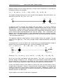
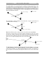
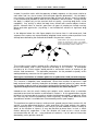
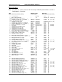
Download Coda AMPLIFIER 15.0 User guide

CODA cx1
User Guide
Charnwood Dynamics Limited
Victoria Mills, Fowke Street,
Rothley, Leicestershire, LE7 7PJ
England
Tel: +44 (0) 116 230 1060
Fax: +44 (0) 116 230 1857
Email: [email protected]
Web: http://www.codamotion.com
1/162
CONTENTS
Introduction
Hardware
Software
PART I - CODA BASICS
1.
Setting Up and Using the System
Coda cx1 Scanner Units
Siting the Scanner Units
Interconnections
Front Panel
Computer
Computer Specification – Mini Hub Operation
Computer Specification – Active Hub Operation
Mini Hub Unit
Active Hub Unit
Software Components
System Configuration: Codasys.cfg
Start-up and Shut-down Procedures
Coda Markers and Drive Boxes
2-Marker Drive Boxes
8-Marker Drive Boxes
Operation
Recharging the Marker Drive Boxes
Using the Markers
Attaching the Markers
Aligning the Coda cx1 Scanner Units
Origin Offset
Aligning a Single Coda
Aligning Two Codas
Aligning Multiple Codas
2/162
Charnwood Dynamics Motion Analysis
Force Platforms (Option)
Hardware
Configuration
EMG (Option)
Real-time Data Display
Marker Positions
Stick-figure View
Force-plate Data
EMG Data
ADC Data
Input Signal Data
Digital Video Capture (Option)
Interfacing with other Equipment (Option)
2.
Using the Codamotion Analysis Software
Codamotion Analysis Basics
The Codamotion Analysis Window
Working with Data Files
Working with Views
Preparing for Data Acquisition
Acquiring Data
The Setup
What is the Setup?
Loading a Setup
Saving a Setup
Modifying an Existing Setup
Using Meaningful Marker Names
Working with Multiple Views in a Setup
Semi-automatic Setup Loading
Stick Figure Views
Animating the stick figure
Viewing the stick figure from different directions
Enlarging or reducing the stick figure
Displaying the whole data set (or some part) in stick figures
3/162
Charnwood Dynamics Motion Analysis
Graph View
Working with plots
Working with cursors
Using static bars
Expanding the data set
Using data filtering
Comments View
Entering comments
Editing comments
Variables
Creating and deleting variables
Defining variables
Viewing defined variables
Exporting variables to other Windows applications
4/162
Charnwood Dynamics Motion Analysis
PART II - GAIT ANALYSIS
1.
Segmental Gait Analysis (3-D)
Overview
Marker Names
Segmental Gait Analysis
Basic Gait Analysis (external)
Marker placement
Unilateral data acquisition
Bilateral acquisition – Right side
Bilateral acquisition – Left side
Segment Reference Points
Segment Embedded Coordinate Frames
Derivations of 3D Segments and Joints from Marker Placements
Derivation of Segment Definitions from Marker Positions
Segment Rotations
Segment Data Types and Channels
Patient Data File
2.
Gait Analysis Report Generation
Required Application files
Overview
Procedure I - in Codamotion Analysis
Procedure II - in MotionDB Report Generator
Changing the scales on the report graphs
Copying the Gait Parameters to an external database
Using different Report configurations
5/162
Charnwood Dynamics Motion Analysis
3.
A Typical Session in the Gait Laboratory
Movement Data Acquisition
Analysis and Report
Further Analysis
6/162
Charnwood Dynamics Motion Analysis
PART III - ADVANCED TOPICS
1.
Using Virtual Markers
Introduction
Definition
Assigning weights by model design (first category)
Centres of mass
Solving the localization of a known point into a rigid marker triad (second
category)
Validity
Having successfully defined some Virtual Markers…
2.
Using Vector Angles
Defining two vectors
Vectors on Stick Figures
3D Vector Angles
2D Vector Angles
3D angle on a stick figure view
3.
Segment Rotations - The Mathematics of Euler Angles
Background
Eulerian System
Choosing the Axis Sequence
Yaw, Pitch and Roll
Mathematical decomposition
Neutral alignments
Coda implementation
Notes and References
4.
Segmental Analysis - Inverse Dynamics
Ankle Moments
Knee and Hip Moments
5.
Enhancing Segment Representation
Single marker representation
Two-marker representation
Three-marker (triad) representation
Over-determination of segments using 4 or more markers
The case for pre-dynamic, or ‘static’ acquisition
7/162
Charnwood Dynamics Motion Analysis
PART IV - REFERENCE
1.
Codamotion Analysis: User Interface Reference
Main Frame
Toolbar
Menu Commands
Keyboard controls
Views
2.
Movement Data File (MDF) Format
Summary
Identifier
Header
Data
Data array types
Data-type Notes
Calculated data
3.
Text Data File (TXT) Format
Summary
Saving data in Text format
Loading Text data
Coordinates
Example Text data
4.
File Types Summary
MDF - Movement Data File
STP – Setup File
MDR – Movement Data Report File
PD – Patient Data File
PDB – MDB Report Generator ‘Patient Database’ and Graph Definition File
CFG – (Report.CFG) MDB Report Configuration File
RPT – Report Template Definition File
5.
Project Setup and Data Types
The Project Setup Configuration
Data Types
8/162
Charnwood Dynamics Motion Analysis
6.
Digital Event Input-Output
Event Recording and Acquisition Triggering Outputs
Real-time Display
Digital Trigger Outputs
Special Input-Outputs
Pin-outs for Digital I/O
9/162
Charnwood Dynamics Ltd.
Coda cx1 User Guide
Introduction
One of the many benefits conferred upon Codamotion users is the economy of effort
resulting from the many time-saving features and overall user-friendliness of the system.
In spite of this, the task of installing and configuring the system for the first time may seem
a daunting one.
The flexibility of the Codamotion system is such that the user may have chosen options
ranging from a single Coda cx1 scanner unit, to a ‘full house’ comprising several
scanners, simultaneous video capture, twin force platforms, optically telemetered EMG
and, perhaps, digital triggers, all kept in check by the powerful Codamotion Analysis
software running on a suitably configured computer with a Microsoft Windows TM based
operating system.
It is essential, therefore, that you read this user-guide very thoroughly, at least to the end
of the first part, before embarking upon any campaign of movement analysis.
Hardware
The Coda cx1 is a general-purpose 3-D Motion tracking system, with interfacing for
synchronous analogue and digital data acquisition (e.g. Force-plate, EMG).
The measurement unit contains three pre-aligned solid-state cameras which track the
position of a number of active markers (infra-red LEDs) in real-time.
Sampling rates
Sampling rates are selectable from 1Hz up to the upper limits defined below for different
numbers of markers in use.
100Hz for up to 56 markers
200Hz for up to 28 markers
400Hz for up to 12 markers
800Hz for up to 6 markers
Measurement time
The maximum measurement time depends on a combination of the sampling rate and the
total number of markers being tracked. For example, with 28 markers (sampling rates of
200Hz or below), the maximum measurement times are:
100s at 200Hz, 200s at 100Hz, 400s at 50Hz, 800s at 25Hz, ... to 20000s at 1Hz.
With 12 markers, the sampling rate can be increased to 400Hz while maintaining a
maximum measurement time of 100s. Likewise, with 6 markers at 800Hz, the maximum
measurement time is still 100s.
As the number of markers decreases, the maximum measurement time can be increased
proportionally for a given sampling rate. For example, at 200Hz with only 1 marker, the
maximum measurement time is increased to 2800s.
CX1 USER GUIDE - COMPLETE.doc 26/04/04
10/162
Charnwood Dynamics Ltd.
Coda cx1 User Guide
Resolution
The angular resolution of each camera is about 0.03 mrad (0.002 degrees); this results in
a lateral position resolution of about 0.05mm at 3 metres distance (horizontally and
vertically), and a distance resolution of about 0.3mm.
Measurement Volume
For standard markers, the measurement volume extends from a distance of 2.0m to about
6.0m in front of the measurement unit, at a width and height approximately 1.6 times the
distance.
Coordinate system
The long axis of the measurement unit defines the direction of the X-axis (normally
horizontal and parallel to the walk-way). The perpendicular away from the unit defines the
positive Y-axis (normally horizontal, across the walk-way). The other perpendicular
(vertical) defines the Z-axis (positive up).
The positive X-axis is to the right as seen from Coda.
The origin of the coordinate system is offset by the user to any point in the field of view.
PC interface
The Coda measurement unit is connected to the host computer via a serial port interface
(RS-232 or RS-422).
Multiple Codas
The measurement volume may be extended by adding additional measurement units. A
second unit will also allow bilateral data acquisition. When multiple measurement units
are used, all markers are tracked simultaneously by each unit - the maximum number of
markers remains at 56 (at 100Hz). Marker position data from each unit is combined
automatically.
Software
The Codamotion Analysis software provides the user-interface to the Coda hardware for
real-time data display and data acquisition (marker position, analogue Force and EMG),
and also the data processing functions for analysing the data.
The software is designed for general-purpose motion analysis, but special functions for
Clinical Gait analysis are included.
The software allows the user to define (Joint) angles from the relative positions of (any)
markers, and can combine force data to calculate joint moments and powers. Angles may
also be defined relative to the Lab coordinate frame.
Marker velocities and accelerations, and distances between markers are calculated
automatically, and are available for plotting.
CX1 USER GUIDE - COMPLETE.doc 26/04/04
11/162
Charnwood Dynamics Ltd.
Coda cx1 User Guide
Marker position data may be filtered and interpolated before it is used to calculate angles
and other derived data; the filtering bandwidth is user-selectable.
Animated Stick-figure diagrams may be displayed for the view along any of the machine
axes, using user-configured joins between markers. The animation rate is adjustable, and
can be reversed.
Marker position data, force data, EMG data, and all derived data may be plotted on userconfigurable graphs; graphs are auto-scaled and may plot multiple data types. Data may
be plotted against time or against a marker position coordinate. The data range displayed
on the graphs may be zoomed in to any time period.
Two cursors are used to mark data and select variable values; one of these marks the
animation point. The cursors are synchronized across all graphs. Event bars may be
added to mark data. The cursor and bar locations are stored in the data file.
Acquired data is normally stored in a binary format unique to Codamotion Analysis (MDF),
but may also be stored in a text-format suitable for exporting to a spreadsheet or word
processor. (The MDF binary format specification is available to users.) Codamotion
Analysis can read text data files and AMASS C3D files (with some restrictions).
CX1 USER GUIDE - COMPLETE.doc 26/04/04
12/162
Charnwood Dynamics Ltd.
Coda cx1 User Guide – Coda Basics
I-1
SETTING UP AND USING THE SYSTEM
Coda cx1 Scanner Units
Each Coda scanner unit contains three special cameras which detect infra-red pulses of
light emitted by the Coda markers and locate the marker positions with very high
resolution and linearity. The cameras are rigidly mounted in the scanner units so that the
system can be precalibrated by Charnwood Dynamics before delivery to the customer.
This relieves the user of the task of calibrating the system before use. The calibrated
system measures the positions of markers within a three dimensional co-ordinate system
which is fixed in relation to the scanner unit. (The nominal origin is usually relocated by
the user and the orientation of the co-ordinate frame can be reset by an alignment
transform in the software.)
Siting the Scanner Units
If you will be using more than one Coda scanner, a number of extra possibilities arise for
which the siting and alignment issues are considerably more complex. It is advisable to
consult with Charnwood Dynamics before making any structural decisions for the
laboratory.
Each scanner unit should be placed on a solid table or bench, mounted on a suitable
tripod, or attached to a solid wall or ceiling. It is important that the scanner unit(s) should
be solidly fixed with reference to the space which constitutes the field of view. Any small
translational movements will register as unwanted variations of similar magnitude in the
co-ordinate values measured by Coda, and if a scanner unit moves in a rotational sense
about any axis then the resulting variations in co-ordinate values can become quite large
as they are magnified with distance. For example, if a Coda unit tilts by 1mm, the
measured co-ordinate of a marker at 3m distance will change by 30mm. Rotational
stability is especially important when more than one scanner unit is used.
The scanner units do not need to be mounted parallel to the room co-ordinate frame (i.e.
the floor), as a co-ordinate alignment transform can be performed in the software. The
mounting angle of each scanner unit should be chosen to centralize the field-of-view.
If the Coda unit is fixed to a tripod, or to a wall or ceiling fixing, it is also important that no
bending or twisting stress is applied, as this might change the relative alignment of the
cameras and distort the co-ordinate frame.
Interconnections
A single Coda interface cable is supplied with each Coda scanner unit. The cable
provides both the 12V DC power and high speed serial communications link via:
i)
A mini hub unit which in turn is connected to the host computer using a serial
cable.
ii)
An active hub unit consisting of a Charnwood Dynamics Quad UART board and a
Single Board Computer (SBC) connected through a compact PCI (cPCI)
backplane.
The Coda interface cable is fitted with a 26-way high density D plug (male) at each end.
CX1 USER GUIDE - COMPLETE.doc 26/04/04
13/162
Charnwood Dynamics Ltd.
Coda cx1 User Guide – Coda Basics
I-1
This cable should be plugged into the correspondingly marked sockets on the mini hub
bulk head or Quad UART board and Coda scanner unit bulk head respectively.
Front Panel
On the front of each Coda scanner unit there are two LED indicator lights. The green LED
signifies that the power is on. The yellow LED becomes illuminated only when the
scanner unit is actively acquiring marker position data under control of the computer.
Adjacent to the yellow LED is a small window of black IR transmitting glass. Behind this
window are mounted IR emitting LEDs which send out coded pulses of infra-red light to
the markers which are attached to the subject. These coded pulses control the time at
which each marker emits its flash of infra-red light.
Computer
The host computer specification depends on the type of Codamotion system being
considered. More specifically, it depends on whether the Coda cx1 scanner is operated
through a mini hub unit or an active hub unit.
Computer Specification – Mini Hub Operation
When the Coda scanner is operated with a mini hub unit, the host computer can be any
standard desktop or laptop machine running Microsoft Windows 98, NT, ME, 2000 or XP.
A processor speed of at least 500MHz is recommended.
The host PC must have one serial port interface for each Coda cx1 unit; these can be RS232 or RS-422.
Standard RS-232 serial port(s) (normally COM1, COM2) are limited in speed (115k-baud
max) and would normally be used only for a single Coda system. The RS-232 cable must
be less than 10m in length. (The RS-232 cable is non-standard and must be supplied by
Charnwood Dynamics [a jumper is required at the mini hub end].)
RS-422 serial interfaces operate at up to 40 times faster than RS-232 (up to 5M-baud),
and can use longer cables. They are provided by adding a (third party) interface card to
the host PC (PCI), or by the addition of a PCMCIA type II adapter to a laptop computer.
One or two PCI cards can be installed to provide two or four RS-422 interfaces to support
up to four Coda cx1 scanner units. Similarly, one or two PCMCIA adapters can provide
two or four RS-422 interfaces on a laptop, but these are limited to 1M-baud. Special
drivers (from the card manufacturers) must be installed to use RS-422 interfaces which
then appear as standard COM ports - usually COM3, COM4, etc.
When two Coda cx1 units are connected to one mini hub unit, both units must be operated
on the same type of serial interface – it is not possible to run one Coda on RS-232 and the
other on RS-422.
CX1 USER GUIDE - COMPLETE.doc 26/04/04
14/162
Charnwood Dynamics Ltd.
Coda cx1 User Guide – Coda Basics
I-1
Computer Specification – Active Hub Operation
When the Coda scanner is operated with an active hub unit, the host system controller
forms part of the active hub and must be a compact PCI (cPCI) Single Board Computer
(SBC) running Microsoft Windows 2000 or XP. A single slot 3U SBC is recommended
with a processor speed of at least 500MHz.
The SBC connects directly into a 3U cPCI backplane together with a Charnwood
Dynamics Quad UART board. A single Quad UART board can provide up to four RS-422
interfaces to support up to four Coda cx1 scanner units at speeds of up to 5M-baud.
Special drivers (supplied) must be installed to use these RS-422 interfaces which appear
as standard COM ports – usually COM 3, COM 4, etc.
Mini Hub Unit
The mini hub unit is used to provide the 12V DC power and high speed serial
communications link to the Coda scanner unit via the Coda interface cable and then to the
host computer using a serial cable.
Each mini hub bulk head is fitted with two 26-way high density D sockets for connection of
the Coda interface cable(s), two 9-way D sockets for RS-422 serial communication and
two 9-way D sockets for RS-232 serial communication. There are two Coda unit power
on/off switches and associated LED indicator lights. The red LEDs signify that there is
mains power to the mini hub while the green LEDs show power to the Coda scanner
unit(s) is on (the green LEDs are only activated when there is a Coda unit plugged in).
Two sync. sockets are also provided for connection of an additional mini hub unit or for
external sync. triggering.
A single mini hub can support up to two Coda cx1 scanner units on either RS-232 or RS422. When two Coda units are connected to a single mini hub, they are automatically
synchronized (no additional sync. cable is required - the sync. lines are connected inside
the mini hub). When two mini hubs are used to operate three or four Coda cx1 units, the
sync. Out on the first mini hub must be connected to the sync. In on the second mini hub.
Two Coda cx1 units connected to the same mini hub can be operated independently from
different host PCs if required.
Active Hub Unit
The active hub unit can be configured to meet specific customer requirements but is
based around a Single Board Computer (SBC) and Charnwood Dynamics Quad UART
board on a 3U cPCI platform. The active hub provides the 12V DC power and high speed
serial communications link to the Coda scanner unit(s) aswell as enabling overall system
control through the SBC.
Each active hub unit consists of a 4/6 or 8-slot 3U cPCI backplane housed in a full (19
inch) or half rack. Power to the backplane is provided from a front panel mounted power
supply and/or from a power supply fixed inside the rack.
The cPCI backplanes used by Charnwood Dynamics normally have a left hand system
slot. Unless otherwise stated, the SBC must occupy the first slot on the backplane
(reading from the left hand side).
CX1 USER GUIDE - COMPLETE.doc 26/04/04
15/162
Charnwood Dynamics Ltd.
Coda cx1 User Guide – Coda Basics
I-1
The Charnwood Dynamics Quad UART boards are fitted with four 26-way high density D
sockets on the front panel for connection of the Coda interface cable(s). There are four
Coda unit power on/off switches and associated green LED indicator lights. The LEDs
show power to the Coda scanner unit(s) is on (the LEDs are only activated when there is
a Coda unit plugged in). Two sync. sockets are also provided for connection of additional
Quad UART boards or for external sync. triggering.
A single Quad UART board can support up to four Coda cx1 scanner units on RS-422.
When two or more Coda units are connected to a single Quad UART board, they are
automatically synchronized (no additional sync. cable is required – the sync. lines are
connected on the board). When two or more Quad UART boards are used to operate five
or more Coda units, the sync. Out on the first Quad UART board must be connected to
the sync. In on the second Quad UART board.
The active hub can be configured to provide interfacing for analogue and digital data
acquisition (e.g. Force-plate, EMG) using a combination of the Charnwood Dynamics 32channel cPCI filter board and third party 16-bit analogue I/O with digital I/O boards.
Typically, 32/64 analogue input channels and 4/8 analogue output channels can be
supported together with digital I/O.
CX1 USER GUIDE - COMPLETE.doc 26/04/04
16/162
Charnwood Dynamics Ltd.
Coda cx1 User Guide – Coda Basics
I-1
Software Components
The required Codamotion system software will normally be installed on your computer by
Charnwood Dynamics. Shortcuts to the Codamotion Analysis software applications
should be available on the Windows desktop and/or on the Windows Start Menu.
Hardware supported by Codamotion Analysis Software (V6.xx)
•
Up to 8 Coda cx1 units using two cPCI Quad UART boards in an active hub unit.
•
Up to 4 Coda cx1 units using one or two mini hub units.
–
requires one serial interface for each Coda unit.
•
Up to 2 third party 16-bit analogue I/O with digital I/O cPCI boards for Force
platform and/or EMG data acquisition. (Typically 32/64 analogue input channels
and 4/8 analogue output channels can be supported with digital I/O).
•
Up to 2 32–channel cPCI filter boards for use with the above analogue I/O boards.
•
ADC-64 64-channel Analogue Acquisition unit (includes 15-channel Digital I/O) for
Force platform and/or EMG data acquisition.
–
requires a DSP32 (mpx30) interface card (one ISA slot in the host PC)
•
Video acquisition from any Video-for-Windows (VfW) compatible device
–
for example, a USB Web Cam.
Data Analysis
To analyse existing data files, you need the following files:
CODA MA6xx_xxx.exe Codamotion Analysis Application program file (Version 6.xx).
CODA MA6xx_xxx.hlp On-line Help documentation.
These files are normally located in a directory named “C:\Codamotion”
There are normally one or more Setup files (*.stp) associated with data files (*.mdf).
These may be located in the main Codamotion folder, or in different project folders.
If there is an “ADemo1.stp” Setup file and an “ADemo1.mdf” data files in the main
Codamotion folder, these may be opened and animated automatically using the Run
Demo command in Codamotion Analysis (Help menu).
Data Acquisition
To acquire data from the Codamotion system, the following additional files are required.
C:\Codamotion\
CodaSys.cfg
- System configuration information file (text)
CX1 USER GUIDE - COMPLETE.doc 26/04/04
17/162
Charnwood Dynamics Ltd.
Coda cx1 User Guide – Coda Basics
I-1
The following files must be in a sub-folder named \Coda:
C:\Codamotion\Coda\
CodaSharc_V3-xx.stk
CX1001-Gains.cx1
CX1001-CalLUT-5.cx1
CX1001-CalGeom.dat
CX1001-CorrelLUT-AL.cx1
CX1001-TemplLUT-A.dat
CX1001-TNormLUT-A.dat
- cx1 DSP program code (Version 3.xx) (hex)
- cx1 calibration data (binary).
- cx1 calibration data (binary).
- cx1 calibration data (text).
- cx1 correlation template (binary).
- cx1 correlation template (hex).
- cx1 correlation template data (hex).
This list shows the files for Coda cx1 serial number 1001. If there is more than one Coda
unit there must be a set of six calibration files for each unit.
Force Platforms
If force platform(s) are to be used, the following files must also be present in the Coda
sub-folder :
C:\Codamotion\Coda\
ForcePlate1.cal
ForcePlate2.cal
Kistler_9281.fp
AMTI_0000.cal
AMTI_AccuGait-0000.cal
- Forceplate 1 calibration data (mV-to-Newtons) (text)
- Forceplate 2 calibration data (mV-to-Newtons) (text)
- Kistler Forceplate CoP correction parameters
- AMTI Forceplate parameter file and calibration matrix
(s/n 0000) (text)
- AMTI Portable Forceplate parameter file and
calibration matrix (s/n 0000) (text)
ADC-64 Analogue Data Acquisition
To acquire data from an ADC-64 Analogue Acquisition unit, the following files must be
present in the Coda sub-folder:
C:\Codamotion\Coda\
CodaSys.dat
ADC64v7B.out
ADC64_000.dat
( Coda.reg
- Coda SDK configuration (DSP interface) (text)
- ADC DSP program file (Version 7B) (binary)
- ADC64 calibration data (mV) (Unit s/n 000) (text)
- Windows Registry entry data (text) )
There must also be a Coda SDK device driver file located in the Windows System
directory. This is either Coda95.dll for Windows 98/ME, or CODAmpx30.sys for Windows
NT/2000/XP:
or
\Windows\System\Coda95.dll
\WINNT\system32\drivers\CODAmpx30.sys
This driver is required for communication with the ADC-64 DSP ISA interface card.
CX1 USER GUIDE - COMPLETE.doc 26/04/04
18/162
Charnwood Dynamics Ltd.
Coda cx1 User Guide – Coda Basics
I-1
Software Installation
If an ADC-64 unit (on an ISA DSP card interface) is not to be used with the system, then
software installation is merely a matter of copying the files into the appropriate directories
(e.g. \Codamotion and \Codamotion\Coda).
When installing files from an installation CD, the system configuration file on the CD is
normally named Codasys_XXX.cfg (where XXX identifies the installation location) so that
if the Codamotion Analysis program is run directly from the CD, it does not try to initiate
the hardware. After copying this file onto the PC’s disk, it must be re-named Codasys.cfg,
and may require editing to setup the serial interface channels correctly (see below).
If an ADC-64 Analogue unit is included in the system, then in addition to copying files into
the appropriate directories, some Windows Registry entries need to be created. This can
be done by double-clicking the Coda.reg file, if any, or by manually editing the Registry:
For all Windows versions:
[HKEY_LOCAL_MACHINE\Software\CODA]
SystemDir=C:\\Codamotion\\coda [string]
For Windows NT/2000/XP (using the CODAmpx30 device driver):
[HKEY_LOCAL_MACHINE\SYSTEM\CurrentControlSet\Services\CODAmpx30]
Type=0x0001
[dword]
Start=0x0002
[dword]
Group=Extended Base [string]
ErrorControl=0x0001 [dword]
[DSP]
Number=0x0001
[dword]
Address1=0x02C0 [dword] (‘2C0’ is the (hex) base address of the ADC-64 DSP
card)
Gait Analysis Report Generation
If you wish to produce clinical gait analysis reports, you will need the MotionDB Report
Generator Application and associated files:
MotionDB V2.24-UK.exe
REPORT.cfg
*.pdb
*.rpt
MotionDB Application program file (Version 2.24-UK)
These files are normally installed in a sub-directory of the Codamotion Analysis
Application: \Report Generator
CX1 USER GUIDE - COMPLETE.doc 26/04/04
19/162
Charnwood Dynamics Ltd.
Coda cx1 User Guide – Coda Basics
I-1
Codamotion Analysis Version
To check the Version number of Codamotion Analysis, either select Help: About
Codamotion Analysis... from the program menu bar, or highlight the Codamotion
Analysis Application (EXE) program file in Explorer and select File: Properties...
Version tab.
Data Files
Data acquired by the Codamotion system is stored in data files on the computer’s hard
disk. These usually have the filename extension ‘.MDF’.
Setup Files
Setup configuration files should have the extension ‘.STP’. Some pre-configured Setup
files are supplied by Charnwood Dynamics.
You may create more Setups files as required; different configurations are required when
markers are used differently, or when data is analysed differently. You should keep your
Setup files in the same directory as the data files to which they apply.
Setup files are text files and may be displayed with any text editor.
Whenever the Codamotion Analysis program is closed, the current Setup is automatically
saved in a temporary file. If present, this setup is loaded automatically next time the
Codamotion Analysis program is started.
CX1 USER GUIDE - COMPLETE.doc 26/04/04
20/162
Charnwood Dynamics Ltd.
Coda cx1 User Guide – Coda Basics
I-1
System Configuration: Codasys.cfg
This file must be present for data acquisition. It specifies the number of Coda cx1 units to
be used for acquisition, the interface type and the serial port(s) configuration(s). It also
specifies the number and configuration of any ADC-64 acquisition units, cPCI data
acquisition boards, Force platforms or EMG units being used. (There is no entry for video
acquisition hardware – this is detected automatically, if present (installed under
Windows)).
If the configuration file is not present in the same folder as the Codamotion Analysis
application program (exe) file, or if it is not named “Codasys.cfg”, then Codamotion
Analysis will not attempt to initialize any hardware and the CODA menu will be
unavailable. All other functions for analysis of existing data files will be available.
In addition to configuration information, the Codasys.cfg file contains text translations of all
the initialization error numbers (these are normally displayed by Codamotion Analysis).
Single Coda system:
:------------------------------------------------------------------: CODA Configuration for CODAmotion Analysis V6.55-CX1 May-2004)
:-------------------------------------------------------------------
[CodaSys]
NumCoda=1
NumADC=0
NumForce=0
NumEMG=0
MarkerType=1
MarkerAcquisition=1
[CODA_1]
SerialNumber=1001
CommPort=5
CodaType=1
Interface=1
:0 for stand-alone ADC, EMG or MA/coda demo/test
:0 disables ADC, 1 enables
:1=Analogue, 2=Digital
:0 to disable marker acquisition
:1=Cx1, 2=Mpx30
:1=MiniHub+BB.RS422, 2=MiniHub+QuadUART.RS422,
3=ActiveHub(cPCI)+QuadUART
CommPacket=0x16
CommRate=11
:11=5.0M, 10=2.5M, 8=1.0M, 7=460k, 4=115.2k, 0=9600
Cameras=3
MaskType=3
:1=PseudoRandom, 2=LinearMask, 3=LinearMask Correlation
Orientation=0
:0=Horizontal 1=Horiz.Inverted 2=Vertical(Top=A) 3=Vertical(Top=C)
DSPProgramFile=CODA\CodaSharc_V3-02.stk
Dual Coda system:
:------------------------------------------------------------------: CODA Configuration for CODAmotion Analysis V6.55-CX1 May-2004)
:-------------------------------------------------------------------
[CodaSys]
NumCoda=2
NumADC=0
NumForce=0
NumEMG=0
MarkerType=1
MarkerAcquisition=1
[CODA_1]
SerialNumber=1001
CommPort=5
CodaType=1
Interface=1
:0 for stand-alone ADC, EMG or MA/coda demo/test
:0 disables ADC, 1 enables
:1=Analogue, 2=Digital
:0 to disable marker acquisition
:1=Cx1, 2=Mpx30
:1=MiniHub+BB.RS422, 2=MiniHub+QuadUART.RS422,
3=ActiveHub(cPCI)+QuadUART
CX1 USER GUIDE - COMPLETE.doc 26/04/04
21/162
Charnwood Dynamics Ltd.
Coda cx1 User Guide – Coda Basics
I-1
CommPacket=0x16
:11=5.0M, 10=2.5M, 8=1.0M, 7=460k, 4=115.2k, 0=9600
CommRate=11
Cameras=3
MaskType=3
:1=PseudoRandom, 2=LinearMask, 3=LinearMask Correlation
Orientation=0
:0=Horizontal 1=Horiz.Inverted 2=Vertical(Top=A) 3=Vert(Top=C)
DSPProgramFile=CODA\CodaSharc_V3-02.stk
[CODA_2]
SerialNumber=1002
CommPort=6
:11=5.0M, 10=2.5M, 8=1.0M, 7=460k, 4=115.2k, 0=9600
CommRate=11
Cameras=3
MaskType=3
:1=PseudoRandom, 2=LinearMask, 3=LinearMask Correlation
Orientation=0
:0=Horiz 1=Horiz.Inverted 2=Vert(Top=A) 3=Vert(Top=C)
DSPProgramFile=CODA\CodaSharc_V3-02.stk
Single Coda system with ADC-64 acquisition unit and Force platforms:
:------------------------------------------------------------------: CODA Configuration for CODAmotion Analysis V6.55-CX1 May-2004)
:-------------------------------------------------------------------
[CodaSys]
NumCoda=1
NumADC=1
NumForce=2
NumEMG=0
MarkerType=1
MarkerAcquisition=1
[CODA_1]
SerialNumber=1001
CommPort=5
CodaType=1
Interface=1
:0 for stand-alone ADC, EMG or MA/coda demo/test
:0 disables ADC, 1 enables
:1=Analogue 2=Digital
:0 to disable marker acquisition
:1=Cx1, 2=Mpx30
:1=MiniHub+BB.RS422, 2=MiniHub+QuadUART.RS422,
3=ActiveHub(cPCI)+QuadUART
CommPacket=0x16
CommRate=11
:11=5.0M, 10=2.5M, 8=1.0M, 7=460k, 4=115.2k, 0=9600
Cameras=3
MaskType=3
:1=PseudoRandom, 2=LinearMask, 3=LinearMask Correlation
Orientation=0
:0=Horiz 1=Horiz.Inverted 2=Vert(Top=A) 3=Vert(Top=C)
DSPProgramFile=CODA\CodaSharc_V3-02.stk
[ADC_1]
:CharnDyn multi-channel ADC/Digital interface
Type=1
:1=ChanrDyn ADC-64, 2=GS-16AIO
SerialNumber=001
DSPboard=0x2C0
DSPProgramFile=CODA\ADC64v7b.OUT
CalFile=CODA\ADC64_001.DAT
[ForcePlate_1]
:Kistler Force platform
Type=1
:0=UserDef 1=9281B 2=9286 3=9261 4=9281C 5=9281C2, 6=9287
Rotation=0
:0,90,180,270 degrees
MatThickness=0
:mm
CentreOffset=0,0,-6
:(x,y,z) mm from origin
ParameterFile=CODA\Kistler9287.fp :Force-plate calibration parameters
CalFile=CODA\FP1.cal
:ADC channel calibration factors
DSPboard=A1:1
:A1:n = ADC_1 channel start n
[ForcePlate_2]
:AMTI Force platform
Type=10
:0=UserDef; 1,2,3,4,5,6=Kistler; 10=AMTI BP2416 11=AMTI LG6
Rotation=0
:0,90,180,270 degrees
MatThickness=0
:mm
CentreOffset=600,0,-6
:(x,y,z) mm from Coda Marker origin
ParameterFile=CODA\AMTI_0000.cal :Force-plate calibration matrix
CalFile=CODA\FP2_000.cal
:ADC channel calibration factors
DSPboard=A1:8
:A1:n = ADC_1 channel start n
CX1 USER GUIDE - COMPLETE.doc 26/04/04
22/162
Charnwood Dynamics Ltd.
BridgeVoltage=10.0
AmpGain=4000,8000
Coda cx1 User Guide – Coda Basics
I-1
:AMTI/Bertec bridge excitation voltage (1.0 - 15.0)
:AMTI/Bertec amplifier gain (low, high)
Single Coda system with Portable Force platforms and EMG:
:------------------------------------------------------------------: CODA Configuration for CODAmotion Analysis V6.55-CX1 May-2004)
:-------------------------------------------------------------------
[CodaSys]
NumCoda=1
NumADC=0
NumForce=2
NumEMG=1
MarkerType=1
MarkerAcquisition=1
[CODA_1]
SerialNumber=1001
CommPort=5
CodaType=1
Interface=1
:0 for stand-alone ADC, EMG or MA/coda demo/test
:0 disables ADC, 1 enables
:1=Analogue 2=Digital
:0 to disable marker acquisition
:1=Cx1, 2=Mpx30
:1=MiniHub+BB.RS422, 2=MiniHub+QuadUART.RS422,
3=ActiveHub(cPCI)+QuadUART
CommPacket=0x16
CommRate=11
:11=5.0M, 10=2.5M, 8=1.0M, 7=460k, 4=115.2k, 0=9600
Cameras=3
MaskType=3
:1=PseudoRandom, 2=LinearMask, 3=LinearMask Correlation
Orientation=0
:0=Horiz 1=Horiz.Inverted 2=Vert(Top=A) 3=Vert(Top=C)
DSPProgramFile=CODA\CodaSharc_V3-02.stk
[ForcePlate_1]
:AMTI AccuSway Force platform
Type=20
:20=AMTI AccuSway
Rotation=270
:0,90,180,270 degrees (Cable towards Coda = 270)
MatThickness=0
:mm
CentreOffset=0,0,-6
:(x,y,z) mm from Coda Marker origin
ParameterFile=CODA\AMTI_AccuGait-0202.cal :Parameter file, inc calibration matrix
CommPort=1
:RS232 COM port number
[ForcePlate_2]
:AMTI AccuSway Force platform
Type=20
:20=AMTI AccuSway
Rotation=270
:0,90,180,270 degrees (Cable towards Coda = 270)
MatThickness=0
:mm
CentreOffset=0,0,-6
:(x,y,z) mm from Coda Marker origin
ParameterFile=CODA\AMTI_AccuGait-0203.cal :Parameter file, inc calibration matrix
CommPort=1
:RS232 COM port number
[EMG_1]
Type=3
Transmitters=2
:EMG System
:3=Noraxon Telemyo 2400T
:1-4
Single Coda system with Active Hub Unit, Force Platforms and EMG:
:------------------------------------------------------------------: CODA Configuration for CODAmotion Analysis V6.55-CX1 May-2004)
:-------------------------------------------------------------------
[CodaSys]
NumCoda=1
NumADC=1
NumForce=2
NumEMG=0
MarkerType=1
MarkerAcquisition=1
:0 for stand-alone ADC, EMG or MA/coda demo/test
:0 disables ADC, 1 enables
:1=Analogue 2=Digital
:0 to disable marker acquisition
[CODA_1]
SerialNumber=1001
CommPort=5
CX1 USER GUIDE - COMPLETE.doc 26/04/04
23/162
Charnwood Dynamics Ltd.
CodaType=1
Interface=3
Coda cx1 User Guide – Coda Basics
I-1
:1=Cx1, 2=Mpx30
:1=MiniHub+BB.RS422, 2=MiniHub+QuadUART.RS422,
3=ActiveHub(cPCI)+QuadUART
CommPacket=0x16
:11=5.0M, 10=2.5M, 8=1.0M, 7=460k, 4=115.2k, 0=9600
CommRate=11
Cameras=3
MaskType=3
:1=PseudoRandom, 2=LinearMask, 3=LinearMask Correlation
:0=Horiz 1=Horiz.Inverted 2=Vert(Top=A) 3=Vert(Top=C)
Orientation=0
DSPProgramFile=CODA\CodaSharc_V3-02.stk
[ADC_1]
Type=2
SerialNumber=000
NumAnalogue=64
NumDigital=32
InputRange=1,2
:CharnDyn multi-channel ADC/Digital interface
:1=CharnDyn ADC-64, 2=GS-16AIO
:0=+/-2.5V, 1=+/-5.0V, 2=+/-10.0V for each 32-channel group
[ForcePlate_1]
:8-channel A/D interface
Type=12
:12=AMTI-OR6-7
:0,90,180,270 degrees
Rotation=0
MatThickness=0
:mm
:(x,y,z) mm from Coda Marker origin
CentreOffset=0,0,-6
ParameterFile=CODA\AMTI_OR6-7-4372.cal :Parameter file, inc calibration matrix
CalFile=CODA\FP1_000.cal :ADC channel calibration factors
DSPboard=A1:33
:A1:n = ADC_1 channel start n
BridgeVoltage=10.0
:AMTI/Bertec bridge excitation voltage (1.0 - 15.0)
AmpGain=4000,8000
:AMTI/Bertec amplifier gain (low, high)
[ForcePlate_2]
:8-channel A/D interface
Type=12
:12=AMTI-OR6-7
Rotation=0
:0,90,180,270 degrees
MatThickness=0
:mm
CentreOffset=0,0,-6
:(x,y,z) mm from Coda Marker origin
ParameterFile=CODA\AMTI_OR6-7-4373.cal :Parameter file, inc calibration matrix
CalFile=CODA\FP2_000.cal :ADC channel calibration factors
DSPboard=A1:39
:A1:n = ADC_1 channel start n
BridgeVoltage=10.0
:AMTI/Bertec bridge excitation voltage (1.0 - 15.0)
AmpGain=4000,8000
:AMTI/Bertec amplifier gain (low, high)
CX1 USER GUIDE - COMPLETE.doc 26/04/04
24/162
Charnwood Dynamics Ltd.
Coda cx1 User Guide – Coda Basics
I-1
[CodaSys]
NumCoda
The number of Coda units configured for data acquisition. If you have two
Codas, you can temporarily de-configure [CODA_2] by setting NumCoda=1.
NumADC
Enables or disables the ADC-64 analogue acquisition unit or cPCI A/D board(s).
NumForce
Specifies the number of force platforms in use.
NumEMG
Specifies the number of EMG systems in use.
Marker Type
The type of marker drive boxes being used (1=Analogue, 2=Digital)
Marker
Acquisition
Enables or disables marker acquisition – normally=1.
[CODA_1]
(or [CODA_2])
SerialNumber
This number must match the number of your Coda cx1 unit. It is used to check
that the calibration files match the unit.
CommPort
The serial communications port being used on the host computer, laptop or
active hub (1=COM1, 2=COM2…, etc.) for Coda cx1 unit connection.
CodaType
The type of Coda unit configured for acquisition (1=cx1, 2=mpx30)
Interface
The serial communication interface type being used with the system
(1=MiniHub+BB RS422 card, 2=MiniHub+QuadUART RS422 card,
3=ActiveHub(cPCI)+QuadUART board)
CommPacket
The serial communication packet size in hexidecimal notation – normally =
0x16.
CommRate
The baud rate for serial communication (11=5Mbaud, 10=2.5Mbaud…,
8=1Mbaud, 7=460kbaud…, 4=115.2kbaud, etc.)
Cameras
The number of cameras being used in the Coda cx1 scanner unit - normally=3.
MaskType
The type of mask fitted to the Coda camera array (1=Pseudo Random, 2=Linear
Mask, 3=Linear Mask Correlation) – normally=3.
Orientation
The default orientation of the Coda scanner unit with respect to the floor
(0=Horizontal, 1=Horizontal Inverted, 2=Vertical – A camera top, 3=Vertical – C
Camera top). This is overridden by the alignment procedure.
DSPProgramFile The program code file which is down-loaded to the SHARC processor. This
may change when you receive software upgrades.
[ADC_1]
Type
The type of data acquisition board/unit configured (1=CharnDyn ADC-64,
2=GS-16AIO).
SerialNumber
The ADC-64 acquisition unit serial number.
NumAnalogue
Specifies the number of analogue channels configured on the active hub.
NumDigital
Specifies the number of digital channels configured on the active hub.
InputRange
The input voltage range for each 32 channel group configured on the active hub
(0=+/-2.5V, 1=+/-5.0V, 2=+/-10.0V).
DSPboard
The PC I/O base address of the DSP32C interface card to which the ADC-64
unit is connected.
CX1 USER GUIDE - COMPLETE.doc 26/04/04
25/162
Charnwood Dynamics Ltd.
Coda cx1 User Guide – Coda Basics
I-1
DSPProgramFile The program code file which is down-loaded to the DSP32C processor. This
may change when you receive software upgrades.
CalFile
ADC-64 calibration data file (gains and offsets).
CX1 USER GUIDE - COMPLETE.doc 26/04/04
26/162
Charnwood Dynamics Ltd.
Coda cx1 User Guide – Coda Basics
I-1
[ForcePlate_1]
(and [ForcePlate_2])
Type
Force Plate type: 0=User defined, 1=9281B Kistler, 2=9286 Kistler…, 10=AMTI
BP2416, 11=AMTI-LG6, 12=AMTI-OR6-7, 20=AMTI AccuSway/AccuGait, etc.
Rotation
The orientation of the plate relative to Coda. May be 0, 90, 180, or 270 degrees
relative to normal (Force-plate x-axis = Coda Y-axis (perpendicular horizontal),
y-axis = X-axis (parallel horizontal), x-axis = Z-axis (vertical)).
MatThickness
The thickness of any covering attached to the surface of the force plate.
CentreOffset
Distance (x,y,z) in mm from the Coda marker origin.
ParameterFile
Force plate calibration parameters. (Centre of pressure correction coefficients
for Kistler force plates; Calibration matrix for AMTI force plates).
CalFile
ADC channel calibration factors (Force plate gains and offsets).
DSPboard
The ADC-64 acquisition unit or cPCI A/D board to which the force plate is
connected together with the channel start number (A1:1=ADC_1:Channel start
1…, etc).
BridgeVoltage
The AMTI/Bertec bridge excitation voltage (1.0 – 15.0).
AmpGain
The AMTI/Bertec amplifier gain (low, high).
CommPort
The serial communications port being used on the host computer, laptop or
active hub (1=COM1, 2=COM2…, etc.) for portable force plate connection.
[EMG_1]
Type
EMG system type: 3=Noraxon Telemyo 2400T.
Transmitters
Specifies the maximum number of transmitters in use.
CX1 USER GUIDE - COMPLETE.doc 26/04/04
27/162
Charnwood Dynamics Ltd.
Coda cx1 User Guide – Coda Basics
I-1
Start-up and Shut-down Procedures
Start-up
After ensuring all system hardware elements are connected appropriately, follow the startup procedure listed below:
1. Switch on power to the computer and monitor, and allow Microsoft Windows to
start.
2. Switch on the Coda cx1 scanner units from the bulk head of the mini hub or the
front panel of the Quad UART board, checking the green LED is on for each unit.
3. When Windows has completed loading you can launch the Charnwood Dynamics
Codamotion Analysis software.
4. The system is now ready to use as soon as you have attached the markers to the
subject whose movements you wish to measure.
Note that if you do not wish to acquire movement data but want to review or analyse data
files already acquired it is not necessary to switch on the Coda cx1 scanner units.
Shut-down
At the end of your measurement session first remember to PUT THE MARKER DRIVE
BOXES ON CHARGE, and then:
1. Exit the Codamotion Analysis Software.
2. Switch off the Coda scanner unit(s) at the mini hub or Quad UART board.
3. Shut down the computer.
Coda Markers and Marker Drive Boxes
The markers which are tracked by the Coda scanner units are small infra-red light emitting
diodes (LEDs). They are available in three sizes; standard, mini and micro.
The LED markers are powered from small drive boxes which are available in two sizes; 2marker or 8-marker. All the drive boxes contain sophisticated circuitry which responds to
infra-red synchronising pulses sent out from the Coda scanner units. The circuitry flashes
the markers at an appropriate point in the time multiplexed sequence which corresponds
with the marker numbers on the box. This is how the system maintains intrinsic marker
identity.
2-Marker Drive Boxes
The 2-marker drive boxes are powered internally by rechargeable button cell batteries.
Each drive box has 2 small sockets into which individual markers can be plugged. Next to
each socket is a number which indicates the identity of the marker which is plugged into
that socket. Note that the markers do not intrinsically carry any particular identification,
they take on the identity of whichever drive box numbered socket they are plugged into.
CX1 USER GUIDE - COMPLETE.doc 26/04/04
28/162
Charnwood Dynamics Ltd.
Coda cx1 User Guide – Coda Basics
I-1
8-Marker Drive Boxes
The 8-marker drive boxes can be powered either internally with rechargeable cells or
externally from a 5 volt power pack. Each drive box has 8 small sockets into which
individual markers can be plugged. A hex switch on the 8-marker drive box allows the
operator to select which group of 8-marker identification numbers will apply to the markers
connected to that box. Up to 56 markers can be used at any one time. The 8-marker
drive box switch settings are shown below:
Primary Settings:
1
2
3
4
8
Coda Mode
Acquisition Rate (max)
12/28/56*
400/200/100Hz*
1
-
9
- 16
28/56
200/100HZ
17 - 24
28/56
200/100Hz
25 - 32
56**
100Hz**
33 - 40
56
100Hz
41 - 48
56
100Hz
49 - 56
56
100Hz
Coda Mode
Acquisition Rate (max)
12/28/56
400/200/100Hz.
13 - 20
28/56
200Hz max.
21 - 28
28/56
200Hz max.
29 - 36
56
100Hz max.
37 - 44
56
100Hz max.
45 - 52
56
100Hz max.
Secondary Settings:
1
2
3
4
NOT USED
5 - 12
NOT USED
If any markers are connected above the maximum number allowed at the selected Coda
acquisition rate, they will interefere with lower-number markers in an unpredictable way –
the drive boxes are not automatically disabled if Coda is operating at too high a rate for
the selected marker number range.
* If a 1-8 drive box is used at 800Hz (with markers 1-6), the markers will be visible in
alternate epochs only. (And if markers 7 or 8 are connected, they will interfere with other
markers (marker 8 may appear as marker 1 in the other alternate epochs).)
** If a 25-32 drive box is used at 200Hz (with markers 25-28), the markers will be visible in
alternate epochs only. (And if Markers 29-32 are connected, they will interfere with other
markers.)
CX1 USER GUIDE - COMPLETE.doc 26/04/04
29/162
Charnwood Dynamics Ltd.
Coda cx1 User Guide – Coda Basics
I-1
Operation
When the scanner unit is not acquiring data (i.e. when the yellow LED on the scanner unit
is not illuminated) very little current is being drawn from the batteries in the drive boxes.
However, as soon as the scanner unit starts to send out control signals to the marker
drive boxes (i.e. with the yellow LED now on) the rate of current consumption rises to
about 50mA in each of the drive boxes if they have two LED markers attached. This
current is principally used by the marker LEDs which are being pulsed with current pulses
of duration 40 microseconds at up to 800Hz repetition rate. The capacity of the batteries
in the drive boxes is 30mA hours. This is sufficient for at least 100 data acquisition runs
before the batteries need to be recharged.
Recharging the Marker Drive Boxes
Recharging should be done by first ensuring that both LED markers are disconnected
from the drive boxes. The drive boxes should then be placed in the charger unit for
overnight charge at the end of each working day. To do this, place each drive box in a
charging bay of the charger unit, ensuring that the prongs of the charging connector are
properly inserted into one of the sockets on the drive box. It does not matter which of the
two sockets are used. Proper connection is confirmed by the red LED above the charger
bay. When all the drive boxes have been placed in the charger unit you should initiate the
12 hour charge cycle by pressing the red button marked ‘Start’. You will see the LED
adjacent to the Start button light up. When the 12 hour charge cycle is complete this LED
goes out and the unit is then in trickle charge mode.
When the Codamotion system is not in use the marker drive boxes should be left in the
charger unit and the charger unit should always be left switched on. This ensures that the
batteries are kept in a full state of charge ready for their next period of use. Never leave
the marker drive boxes unconnected to the charger after use as the small current which
the internal circuitry uses, combined with the battery’s self discharge will mean that the
batteries run down within a few hours. It is quite safe to leave the batteries on trickle
charge indefinitely.
Using the Markers
When using the markers for acquiring movement data it is important to understand that
the Coda scanner unit must have an unimpeded view of the LED markers and their drive
boxes. Both the drive boxes and the LEDs have a field of view which encompasses a
solid angle of 180 degrees.
This is more than adequate for most applications. However it is important to be aware
that if the LED markers or the drive boxes are rotated to the limit of their angular field in
relation to the scanner unit then the markers may disappear from the view of the system.
Attaching the Markers
Markers and their associated drive boxes are attached to the subject being studied using
medical double sided adhesive tape. It is recommended that careful thought is given to
the siting of markers before starting to mount them on the subject. The field of view
considerations noted above and the relative siting of markers and drive boxes should be
taken into account. To assist in this, LED markers are provided with leads of different
lengths so that the appropriate length lead can be chosen to suit a given site on a subject
of particular size. Also bear in mind that it is quite permissible to use only one LED
marker with any drive box if connecting two is not convenient in a particular situation.
CX1 USER GUIDE - COMPLETE.doc 26/04/04
30/162
Charnwood Dynamics Ltd.
Coda cx1 User Guide – Coda Basics
I-1
Care should be exercised not to pull too strongly on the thin flexible leads of the LED
markers. They are quite strong but there is obviously a limit to the strain they can
withstand before being damaged. Particular care should be taken when removing
markers and drive boxes from the subject after a measurement session. It is advised that
the LED connectors should be removed from the drive box sockets before the markers or
drive boxes are pulled from the adhesive tape which attaches them to the subject. This
will minimise the risk of accidentally over-stressing the leads.
CX1 USER GUIDE - COMPLETE.doc 26/04/04
31/162
Charnwood Dynamics Ltd.
Coda cx1 User Guide – Coda Basics
I-1
Aligning the Coda cx1 Scanner Units
The Codamotion Analysis program applies an offset and rotational transformation to the
co-ordinates measured by each Coda, so as to reference them to a common room coordinate frame.
When a single Coda unit is in use, the rotational transformation is optional, but the origin
offset must be set for each measurement session (each time Codamotion Analysis is
started). The origin location is not stored. The program will normally not allow data
acquisition until the origin has been set (using the CODA: Define Marker Origin
command). †
When two or more Codas are used together, both the origin offset and rotational transform
must be applied to ensure that the co-ordinates measured by each unit are referenced to
a common co-ordinate frame.
Origin Offset
The origin offset may be reset at any time, and is independent of any rotational
transformation.
The origin point must be within the field of view of all active Codas, and it must be
possible to place a marker at this point which can be seen clearly by all active Codas
simultaneously. The marker must not be too oblique to any Coda, and there should not
be any reflecting surfaces close by. The origin point should be approximately equidistant
from all active Codas. When a force platform is in use, the origin must be set at its centre.
Any marker may be used to define the origin: select the Define Marker Origin…
command from the CODA menu and enter the marker number. When OK is pressed, the
marker position is measured a number of times to average any co-ordinate noise. If the
marker does not provide a strong enough signal, the operation will fail.
Aligning a Single Coda
A single Coda may be aligned to a room (walkway) co-ordinate frame either physically or
by creating an alignment transformation (rotation) matrix.
If an alignment transform matrix is created, it is stored in a text file
C:\Codamotion\Coda\CXxxxx-Alignment.dat (where xxxx is the Coda unit serial number)
and can be used in subsequent measurement sessions if the Coda has not been moved.
Physical Alignment
The Coda’s co-ordinate frame is accurately aligned with its front plate: the x-axis is the
sideways (long) axis, positive to Coda’s right, the y-axis points forwards, and the z-axis
upward.
The Coda unit may be adjusted physically to the room (walkway) co-ordinate frame using
a spirit level, tape measure etc. Alternatively, place three markers in a triangular pattern
†
It is possible to configure Codamotion Analysis to allow data acquisition without having set an origin by
editing the application’s initialization profile (its INI file in the WINDOWS directory): set the ‘NoConfirmInit’
value in the [AppOptions] section to ‘1’. If an origin has not been set, acquired co-ordinates will be relative to
a point behind Coda’s ‘A’ camera.
CX1 USER GUIDE - COMPLETE.doc 26/04/04
32/162
Charnwood Dynamics Ltd.
Coda cx1 User Guide – Coda Basics
I-1
on the walkway in front of Coda (two on the x-axis and one on the y-axis), and observe
their co-ordinates with the real-time co-ordinate display (CODA: Display Marker
Positions…). Rotate Coda about a vertical axis to equalize the y-co-ordinates of the xaxis markers, and adjust Coda’s feet to equalize the z-co-ordinates of all markers. Reset
the marker origin periodically to facilitate comparison of the co-ordinates.
Creating an Alignment Transform
This allows the Coda to be used in an arbitrary (fixed) orientation to the room (walkway)
co-ordinates:
By placing markers in the field of view which define the room X-axis and Y or Z axis, an
alignment transformation (rotation) matrix can be created and stored which can be applied
to all subsequent measurements:
Place one marker at your origin, and another at a point on your new X-axis at least
500mm away from the origin in the positive direction. A third marker may be placed on
the negative X-axis (at least 500mm from the origin) to improve the accuracy of the
alignment.
Place another marker at a point on one of your lateral axes (Y or Z), at least 500mm away
from the origin in the positive direction. In conjunction with the X-axis markers, this
marker is used to define the principal plane of your co-ordinate system (the X-Y plane or
X-Z plane), but does not have to be placed exactly on the lateral axis, as this axis will be
made orthogonal to the X-axis automatically. Another marker may be placed in the
principal plane near the negative lateral axis (at least 500mm from the origin) to improve
the accuracy of the principal plane.
It is not necessary to mark the third axis, as this is automatically generated as a line
through the origin perpendicular to the principal plane, in a direction which defines a righthanded co-ordinate system.
All markers should be placed facing Coda, and there should be no reflecting surfaces
nearby.
Open the Align Coda Co-ordinates dialog by selecting the Align Coda… command on
the CODA menu, and enter the marker numbers in the appropriate boxes. If you have
used only two markers per axis, then enter the origin marker as the first (‘-‘) marker for
each axis.
Press OK to generate and store an alignment transform matrix.
If the marker positions are inconsistent, an error message will be given.
When placing the marker(s) to define the lateral axis, be sure to place it on the correct
side of the origin so as to define the third axis in the required direction. If you stand facing
along the positive X-axis and place the Y-axis marker on your left, the Z-axis will be
positive upwards to give a right-handed co-ordinate frame. (If the lateral axis marker
defines the Z-axis and is on your left, then the Y-axis will be positive downwards.)
CX1 USER GUIDE - COMPLETE.doc 26/04/04
33/162
Charnwood Dynamics Ltd.
Coda cx1 User Guide – Coda Basics
I-1
In the Alignment dialog, there is a box in which to specify an ID name for the alignment
transform matrix. At present (May 2003), only one transform matrix may be stored, so this
box is disabled – the transform matrix is labelled ‘CodaAlignment’.
The alignment transform matrix is stored in the text file CXxxxx-Alignment.dat (where xxxx
is the Coda unit serial number) in the C:\Codamotion\Coda\ directory, and is loaded (only)
when Codamotion Analysis is started. If desired, you can place your own transformation
(rotation) matrix in this file. The matrix must be orthogonal – if not, Coda initialization will
fail with error 156.
Using an Alignment Transform
The use of a (stored) alignment transform when displaying or acquiring marker coordinates is determined in the Acquisition Setup dialog by the Co-ordinate Transform
selection (CODA menu: Acquisition Setup… command).
After creating and storing an alignment transform, the Co-ordinate Transform selection is
automatically set to ‘CodaAlignment’.
To switch off co-ordinate transformation, select ‘none’ in the Co-ordinate Transform box.
If a co-ordinate transform is selected, it is listed in the message box which appears just
before data acquisition is started.
The Co-ordinate Transform selection (‘none’ or ‘CodaAlignment’) is saved with all other
acquisition options when the Setup is saved (Setup: Save Setup…)
If there is no stored alignment transform available, the Co-ordinate Transform selection
box will have only ‘none’ available.
When a co-ordinate transformation is in use, it (and the origin offset) is applied to the
Coda co-ordinates before they are stored after data acquisition. The stored data cannot
be de-transformed.
Remember that the transform matrix will be invalidated by moving Coda.
Aligning Two Codas
Two Codas may be aligned to each other and to a room (walkway) co-ordinate frame
either physically or by creating alignment transformation (rotation) matrices for each Coda.
If alignment transform matrices are created, they are stored in text files
C:\Codamotion\Coda\CXxxxx-Alignment.dat (where xxxx is the Coda unit serial number)
and can be used in subsequent measurement sessions if the Codas have not been
moved.
Physical alignment of two Codas is restricted to making them parallel or perpendicular to
each other, but with an arbitrary offset in all three directions. The field-of-views must
overlap at least at the point where a common origin is to be set (which must be the centre
of any force platform).
CX1 USER GUIDE - COMPLETE.doc 26/04/04
34/162
Charnwood Dynamics Ltd.
Coda cx1 User Guide – Coda Basics
I-1
The choice between parallel/perpendicular alignment and an arbitrary orientation using
alignment transforms is made in the CODA Configuration dialog (CODA menu:
Configuration… command)
If the ‘Aligned’ configuration is selected, then alignment transforms must be available
before data acquisition is allowed.
Parallel or Perpendicular Alignment
Each Coda needs to be physically aligned with the room/walkway in the same way as a
single Coda, using a triangle of markers on the floor.
Both Codas may be aligned to the same triangle of markers if the markers are made
visible to both Codas by placing them flat on the floor. The Real-time marker display
shows separate co-ordinates for each Coda when a Parallel/Perpendicular configuration is
selected.
However, when markers are at a high angle to Coda, the signal received at Coda is
relatively weak and the measured co-ordinates may be inaccurate and noisy. It may be
better to align each Coda with the markers facing each Coda in turn, being careful not to
rotate the axes defined by the markers when they are moved (translation of the axes
doesn’t affect the alignment).
A common origin is set with a single marker when the Origin is defined at the beginning of
each measurement session.
Creating an Alignment Transform
When the Codas are positioned in an arbitrary orientation to the room and/or to each
other, alignment transforms must be created for each Coda in the same way as for a
single Coda.
It is possible to create alignment transforms for both Codas simultaneously if the markers
defining the co-ordinate axes are made visible to both Codas – the Alignment dialog has
check boxes for each Coda. However, this is likely to mean that the markers will be at a
high angle to one or both Codas, which could result in an inaccurate alignment, so it may
be better to align each Coda separately, with markers facing Coda. This also ensures that
the markers will be clearly in view of each Coda during the alignment procedure.
It is not necessary to have a common origin when creating the alignment transforms, as
long as there is no rotation of the marked axes for each Coda. The alignment transform
matrices are purely rotational; a common origin is set independently of the rotational
transform with the Define Marker Origin function (which must be executed at the
beginning of each measurement session).
To ensure that the axes to which each Coda is aligned are parallel, use pairs of markers
stuck together back-to-back, and orientate each pair in the same direction (parallel to the
X-axis). This of course means entering different marker numbers in the alignment dialog
for each Coda.
CX1 USER GUIDE - COMPLETE.doc 26/04/04
35/162
Charnwood Dynamics Ltd.
Coda cx1 User Guide – Coda Basics
I-1
When creating alignment transforms for two Codas, place the marker boxes flat on the
floor. Or, if you get warnings of markers going out of view when aligning each Coda
separately, point the control boxes at each Coda in turn. (This may happen if you are
using the Codas in a very large space with a high ceiling. During the alignment
procedure, each Coda strobes separately.)
Using an Alignment Transform
The use of a (stored) alignment transform when displaying or acquiring marker coordinates is determined in the Acquisition Setup dialog by the Co-ordinate Transform
selection (CODA menu: Acquisition Setup… command).
After creating and storing alignment transforms, the Co-ordinate Transform selection is
automatically set to ‘CodaAlignment’. This selection is stored in the Codamotion Analysis
Setup file (Setup: Save Setup…).
When Codamotion Analysis is started with an ‘Aligned’ configuration of two Codas, the
stored transformation matrices are re-loaded and will be used automatically if the
Acquisition Setup specifies ‘CodaAlignment’ in the Co-ordinate Transform box. Data
acquisition is disabled if the ‘CodaAlignment’ transform is not selected or is unavailable
when using an ‘Aligned’ configuration.
Remember that the transform matrix will be invalid if either Coda has been moved.
There is no automatic warning of misalignment of two Codas, but the real-time marker
display will show a large error value (in the fourth column) for markers visible to both
Codas.
Checking the Alignment
For markers visible to both Codas simultaneously, an error value is displayed in the realtime marker display. This is the Euclidean distance between the co-ordinates of the
marker measured by each Coda. However, for a marker to be visible to both Codas
simultaneously, it may be at a high angle to one or both, and so the co-ordinate value may
be inaccurate.
Aligning Multiple Codas
Multiple Codas must be aligned to each other and to a room (walkway) co-ordinate frame
by creating alignment transformation (rotation) matrices for each Coda.
If alignment transform matrices are created, they are stored in text files
C:\Codamotion\Coda\CXxxxx-Alignment.dat (where xxxx is the Coda unit serial number)
and can be used in subsequent measurement sessions if the Codas have not been
moved.
Creating an Alignment Transform
When the Codas are positioned in an arbitrary orientation to the room and/or to each
other, and the markers defining the co-ordinate axes are made visible to all Codas, it is
possible to create alignment transforms for all Codas simultaneously by selecting the
Align Coda… command on the CODA menu, and checking the appropriate boxes in the
Alignment dialog.
CX1 USER GUIDE - COMPLETE.doc 26/04/04
36/162
Charnwood Dynamics Ltd.
Coda cx1 User Guide – Coda Basics
I-1
However, for the special case with a multi-Coda set-up, where the markers defining the
co-ordinate axes are not visible to all Codas (i.e. the fields of view from each Coda unit do
not sufficiently overlap), then the alignment transforms must be generated using the Align
Multi-Coda system… command on the CODA menu.
This procedure requires the use of a simple alignment jig, manufactured by Charnwood
Dynamics, and is documented separately (Please call Charnwood Dynamics for further
details).
Using an Alignment Transform
The use of a (stored) alignment transform when displaying or acquiring marker coordinates is determined in the Acquisition Setup dialog by the Co-ordinate Transform
selection (CODA menu: Acquisition Setup… command).
After creating and storing alignment transforms, the Co-ordinate Transform selection is
automatically set to ‘CodaAlignment’. This selection is stored in the Codamotion Analysis
Setup file (Setup: Save Setup…).
When Codamotion Analysis is started with an ‘Aligned’ multi-Coda configuration, the
stored transformation matrices are re-loaded and will be used automatically if the
Acquisition Setup specifies ‘CodaAlignment’ in the Co-ordinate Transform box. Data
acquisition is disabled if the ‘CodaAlignment’ transform is not selected or is unavailable
when using an ‘Aligned’ configuration.
Remember that the transform matrix will be invalid if any Coda unit has been moved.
There is no automatic warning of misalignment of Codas.
CX1 USER GUIDE - COMPLETE.doc 26/04/04
37/162
Charnwood Dynamics Ltd.
Coda cx1 User Guide – Coda Basics
I-1
Force Platforms (Option)
Force platforms, which provide analogue outputs, can be interfaced to the Codamotion
system through either an ADC-64 data acquisition unit or a suitably configured cPCI active
hub unit. Portable force platforms can also be supported directly on a serial interface
(RS232 or USB). The Codamotion Analysis software handles the calculations required to
convert raw force signals to force vectors for use in segmental gait analysis. Codamotion
Analysis can be configured to support force platforms manufactured by Kistler, AMTI or
Bertec and portable force platforms made by AMTI.
Hardware
The six or eight output signals from the force platform amplifiers are connected to one of
the analogue input connectors on the ADC-64 unit or the cPCI active hub system. (The
ADC-64 unit is connected to the host PC via an ISA DSP32 interface card). For the case
of the portable force platform, the comms cable plugs directly into the serial port (RS232
or USB) of the host computer.
Configuration
Codamotion Analysis may be configured to use the ADC-64 data acquisition unit or the
cPCI active hub system in the configuration file Codasys.cfg. The configuration file
specifies the ADC-64 serial number, DSP board program file and ADC-64 calibration data
file.
The force platform configuration is also specified in Codasys.cfg and includes: the
platform type (1 = Kistler 9281B, 2 = Kistler 9286, 3 = Kistler 9261…, 10 = AMTI BP2416,
11 = AMTI-LG6, 12 = AMTI-OR6-7, 20 = AccuSway/AccuGait, etc), the calibration file
name (e.g. Coda\FP1.cal), the centre of pressure correction coefficients for Kistler plates,
the calibration matrix for AMTI plates, the ADC-64 unit/cPCI board and channel group to
which the force plate amplifiers are connected (if applicable), the serial port number to
which the force plate is connected (if applicable), the force plate orientation (rotation = 0,
90, 180, 270), the cover-mat thickness (if any), and the centre offset (x,y,z).
Normal orientation is with the long side of the platform parallel to Coda, and with the cable
outlet on the Coda side. The Rotation value for this orientation is 0. The force plate may
be rotated by 90°, 180°, or 270° from the normal orientation - the rotation angle is
clockwise as seen from above.
In all cases, the Coda axes must be aligned exactly parallel/perpendicular to the force
platform axes, in all three directions, and the origin must be set at the specified offset
position relative to the centre of the plate.
CX1 USER GUIDE - COMPLETE.doc 26/04/04
38/162
Charnwood Dynamics Ltd.
Coda cx1 User Guide – Coda Basics
I-1
EMG (Option)
EMG systems can be interfaced through either an ADC-64 data acquisition unit or a
suitably configured cPCI active hub unit to the Codamotion system. In addition, some
EMG systems can now be supported directly from a host PC or laptop using a USB or
PCMCIA interface. Codamotion Analysis can be configured to support EMG systems
manufactured by Motion Lab Systems and Noraxon.
CX1 USER GUIDE - COMPLETE.doc 26/04/04
39/162
Charnwood Dynamics Ltd.
Coda cx1 User Guide – Coda Basics
I-1
Real-time Data Display
There are a number of real-time data display Views. They are opened from the CODA
menu. All Real-time displays are updated at 20Hz.
Real-time Marker Positions (CODA: Display Marker Positions)
This is a text display of marker position (x,y,z) coordinate values. Markers are labelled
by their hardware ID number. The display is updated at 20Hz; coordinates are
displayed only for markers which are in-view.
The maximum number of markers displayed is determined by the current Acquisition
Sampling rate (CODA: Acquisition Setup...). To ensure that all (56) markers are
displayed, set the Sampling rate to 100Hz or less.
If two Codas are connected and configured (Codasys.cfg configuration file and CODA:
Configuration... menu command), the coordinates measured from each unit are
displayed.
Real-time Stick-figure View (CODA: Display Stick-figure)
This is a graphical display of markers joined together according to the current Stickfigure joining diagram defined in the Setup (Setup: Stick-figure Joining Diagram...).
The viewing direction (axis) and view area are set in the Views: Stick-figure Viewing
options... dialogue. The viewing area coordinates are with respect to the current Origin
(CODA: Define Marker Origin...).
The display is updated at 20Hz.
The maximum number of markers displayed is determined by the current Acquisition
Sampling rate (CODA: Acquisition Setup...). To ensure that all (56) markers are
displayed, set the Sampling rate to 100Hz or less. Only one Real-time Stick-figure may
be displayed.
Real-time Force-plate Data (CODA: Display Force-plate)
This is a text display of the 6 / 8 analogue data channels from a Force plate (not the
calculated Force vector data.)
The values displayed have been offset and scaled by the values stored in the Forceplate calibration file (specified in the Codasys.cfg configuration file). Thus they should
read close to zero when no force is applied to the Force plate.
Real-time EMG Data (CODA: Display EMG)
This is a text display of up to 32 analogue data channels from an EMG system. The
values displayed have been offset and scaled by the values stored in the EMG
calibration file (specified in the Codasys.cfg configuration file – if applicable).
Valid data is displayed only if EMG Acquisition has been selected in the Acquisition
Setup (CODA: Acquisition Setup...).
CX1 USER GUIDE - COMPLETE.doc 26/04/04
40/162
Charnwood Dynamics Ltd.
Coda cx1 User Guide – Coda Basics
I-1
Real-time ADC Data (CODA: Display ADC)
This is a text display of 64 channels of analogue data and 15 digital I/O channels.
Available only if an ADC-64 acquisition unit or a cPCI active hub system with
analogue/digital I/O boards is configured [Codasys.cfg].
Real-time Input Signal Data (CODA: Display Input Signal Graphs)
This is a graphical display showing a scrolling chart of analogue, digital or force plate
signals (if configured).
CX1 USER GUIDE - COMPLETE.doc 26/04/04
41/162
Charnwood Dynamics Ltd.
Coda cx1 User Guide – Coda Basics
I-1
Digital Video Capture (Option)
Interfacing with other Equipment (Option)
CX1 USER GUIDE - COMPLETE.doc 26/04/04
42/162
Charnwood Dynamics Ltd.
Coda cx1 User Guide – Coda Basics
I-2
USING THE CODAMOTION ANALYSIS SOFTWARE
Codamotion Analysis Basics
The Codamotion Analysis Window
This is what you see on your screen throughout a Codamotion Analysis session. To begin
a motion analysis session and open the Codamotion Analysis window, double-click the
Codamotion Analysis icon on the desktop (or select it from the Start menu).
At the top of the screen is the title bar, which tells you that this is the Codamotion Analysis
application, as well as the name of the current data file and setup (if any).
Below the menu bar is the toolbar. This has a number of buttons which can be clicked to
execute common Codamotion Analysis tasks.
At the very bottom of the screen is the status bar which displays useful information about
what is going on. It also gives brief instant on-line help for all menu and toolbar
commands.
When you open a data file (see Working with data files), various view windows can be
created within the Codamotion Analysis window. Real-time view windows can also be
created to monitor the Codamotion system hardware in real-time (see Working with
views). Different menu and toolbar options are available depending on which view is
currently highlighted.
Working with Data Files
A data file is the generic term for a collection of data which can be stored on computer
disk. In Codamotion Analysis, a data file contains all of the information about the
movement of markers, and any force plate and/or EMG data. It also contains information
to help in analysis such as the date of acquisition, positions of the left and right cursors,
positions of static bars, and comments which you can add to the file using the Comments
view.
Data files are created in temporary memory whenever you get new data using the acquire
command, but you will normally save the file to disk so that you can refer to it on another
occasion. To acquire a new data file, see Acquiring Data. Once you have done a quick
examination of the data and found that it is acceptable, it is good practice to save the file
straight away. If you try to close a file which you have acquired but not saved, you will be
prompted by a dialogue box asking you whether you wish to save the file before it is
closed.
To Save a Data File
Choose the Save command from the File menu. If you have not saved the data file
before, the File Save As dialogue box will appear. Here, you give the file a unique
name.
If you intend to gather larger numbers of data files (as is usually the case) then you
should adopt a naming convention of some sort, and use the Multiple Acquire/Save
facility. Typical conventions use the initials of the subject, and digits which indicate the
run number. Sometimes, other information is also included in the file name, such as L
or R to represent left or right gait data.
CX1 USER GUIDE - COMPLETE.doc 26/04/04
43/162
Charnwood Dynamics Ltd.
Coda cx1 User Guide – Coda Basics
I-2
It may be sensible to separate different research projects by storing the data files in
different directories on your hard disk. You can select which directory to use from the
directory box in the dialogue box. To find out about creating and managing directories,
see your Windows manuals.
To Open a saved data file
Choose the Open command from the File menu, select the directory in which the file is
stored, and either type or select from the list the name of the file.
Once you have acquired or loaded a data file, various tools are available to help you to
analyse it. You can look at different aspects of the data using different view windows.
Working with Views
Views are windows which appear inside the main Codamotion Analysis window. They
give you a visual display of the data you are looking at, whether it is text or graphs. Any
number and combination of views can be displayed. Two categories of view are available.
There are views which are associated with the current data file, and views which are
associated with the Charnwood Dynamics Codamotion system.
Real time views include: Stick Figure view, and Marker Positions view. The stick figure
view allows you to see in a very graphic way that all markers are correctly positioned on
the subject. The marker positions view gives you figures on the current positions of
markers in all three axes.
The first data file view is the stick figure view. This gives you an overview of marker
positions in two axes in a stick figure form. Several stick figure views can be displayed at
once. When you close the last stick figure view, the whole data file will be closed. For
precise figures on movement, you need to use graph views. Graph views can display
several plots of data, with precise figures underneath. Two additional views are available:
Comments view, which allows you to store comments about the data with the data file;
and variables view, which allows you to examine the values of defined variables.
All of the views in the Codamotion Analysis Window can be arranged by dragging the
windows around the screen, sizing the windows, and using the standard window menu
commands: tile, cascade, and arrange icons.
Preparing for Data Acquisition
Before you begin data acquisition you must set up the Coda machine. Ensure that the
Coda scanners (and any other peripherals such as a force plate amplifier) are switched on
before running the Codamotion Analysis program. If the scanner installation is reliably
firm the alignment of the co-ordinate frame for the acquisition volume may be as minimal
as defining the origin but, if the scanners are prone to physical disturbance between
sessions, it will be necessary to follow the alignment procedure detailed above: see
Alignment of CODA cx1 Scanners.
Markers must be attached to the subject (see below for standard gait analysis marker
placement protocols), and if EMG data is to be recorded the transmitter and electrodes
must also be attached.
CX1 USER GUIDE - COMPLETE.doc 26/04/04
44/162
Charnwood Dynamics Ltd.
Coda cx1 User Guide – Coda Basics
I-2
If you have created a suitable marker joining diagram, or have loaded a setup (see What
is the Setup? for more information) then you can check that markers are correctly
positioned using the Display Stick Figure command from the CODA menu. For a quick
check that all the markers you are using are in view, choose the Display Marker Positions
command. A red arrow will appear next to the numbers of all markers which are in the
field of view of the machine.
If all markers are in view, you are ready to acquire a data file.
Acquiring Data
Acquiring data is the process of storing the movements of markers, force plate data, and
EMG data in the computer’s memory. You can then use the tools provided to analyse the
data.
To acquire data
Choose Acquire Data from the CODA menu, or click the acquire data button on the
toolbar.
In the dialogue box, type the numbers of the markers that you want to acquire.
Select the required sampling rate (normally 200Hz for gait analysis) and then enter the
duration for which you want to acquire data or the number of samples to acquire.
At the 200Hz sampling rate, the acquisition duration is limited to 100s (20000
samples) for 28 active markers. (Acquisition duration can be increased by using
fewer markers). However, you should bear in mind the amount of disk space
required to save the data, especially if you are using a large number of markers, a
force platform, and/or an EMG system.
If the subject is starting from out of the field of view, ensure that the Auto Start option
is selected. This prevents unwanted data from being acquired whilst the subject
moves into the field of view. This also prolongs battery life, as the markers operate at
a reduced sampling rate during stand-by.
Select the Auto End option to stop data acquisition automatically when all markers
pass out of the field of view.
If you are using a force platform, select the Acquire Force data option.
If you are using EMG, you will need to have set the EMG options.
Click on Acquire. If auto start was selected, a dialogue will tell you that the machine is
standing by for markers to come into view. When all the markers enter the field of
view, the machine will start acquiring data, and this will be indicated by the dialogue
box. If the machine fails to start acquiring data it indicates that not all the markers
which you typed into the acquisition dialogue box have come into view.
When acquisition has finished a number of views may be displayed automatically,
depending on the Setup (see below). The acquisition statistics provided by the
(optionally) automatic views: Marker % In View and data Summary are particularly useful.
Stick figure views and/or graphs of the data will be shown, depending on which setup has
been loaded, and whether a suitable Joining Diagram has been defined.
CX1 USER GUIDE - COMPLETE.doc 26/04/04
45/162
Charnwood Dynamics Ltd.
Coda cx1 User Guide – Coda Basics
I-2
The Setup
What is the Setup?
The setup is the set of options which tell the Codamotion Analysis application how you
want data to be displayed, including the set of names assigned to markers and other data
channels. The current setup options apply to all data files which are open. You can
create a standard setup which you can save to a named disk file. Once you have created
a standard setup, you needn’t worry about setup options, you can just load the setup, and
everything will be configured for you. You may be happy with the options in one of the
sample setup files provided with the application: GAIT.STP, and EMG.STP. It is likely that
you will want a separate setup for different research projects. You will need separate
setups for different marker configurations.
If, as advised, you keep all the data files for different research projects in different
directories, then it is sensible to store the appropriate setup files in the same directory.
The first part of the setup simplifies life for you by assigning names to marker, EMG, force,
and force vector channels. This assignment makes other parts of the setup process
easier. For example, if you always place Marker 1 on the ankle, then you can define
Marker 1 as “Ankle”. So when you are creating graphs, for instance, instead of having to
remember which marker is placed on the ankle, you can simply use the name “Ankle” and
the program will know what it means. The same applies to EMG channels. Typically,
customised name assignments for force data are unnecessary, as there is only one force
plate, but you are free to re-assign this if you wish.
Once marker names have been assigned, you can create a stick figure joining diagram.
This defines which markers are connected to which on the real-time and post-acquisition
2D stick figure views.
Another set of options is the definitions of joint angles. This allows you to specify the
markers which are used to define any joint rotation angle. If force data is available, joint
moments and powers can also be calculated. These calculated sets of data can then be
displayed on graphs.
An advanced setup option is the creation of variables, see Variables Overview.
You can create graphs of any data set against time, or against a marker position. Any
graphs which you have configured are also part of the setup. The graphs and their
positions on the screen are saved as part of the setup. At any time you can revert to the
positions of the graphs which were saved with the setup which is currently loaded.
When you start a Codamotion Analysis session, the setup is automatically restored to the
state it was in when you finished your previous session, even if you did not save it as a
setup file. If you are using Codamotion Analysis for the very first time on your computer,
then a default setup is used. You can load a setup at any time with the Load Setup
command in the Setup menu. If you load a setup when a data file is open, then any graph
views which are currently open for that data file will be removed, and new ones will be
created if they are configured in the new setup.
The name of the last-loaded Setup file is displayed at the end of the Codamotion Analysis
title bar. If a Setup file has not been loaded, then “[-]” is displayed.
CX1 USER GUIDE - COMPLETE.doc 26/04/04
46/162
Charnwood Dynamics Ltd.
Coda cx1 User Guide – Coda Basics
I-2
Loading a Setup
This will re-configure all data channels, stick figure views and graph views. If you already
have a data file loaded then any graphs currently displayed for the data file will be
removed, and new ones will be created.
To load a setup:
Choose Load Setup from the Setup menu.
If you keep setup files for different projects or marker configurations in different
directories, then select the correct directory from the directory list in the dialogue box.
Type or select the name of the setup to load, and choose OK.
After loading a Setup file, its name is added to the Codamotion Analysis title bar, e.g.
“[GAIT.STP]”.
Saving a Setup
This will store the current set of marker names, EMG channel names, graph
configurations and options to a setup file which you can load at any time. Before you save
a setup, it is best to arrange the graphs into a clear layout on the screen and to iconize
some if you have a large number. You can do this with the Window menu Cascade and
Tile commands. An iconized view will be stored as such in the setup file.
To save a setup:
Choose Save Setup from the Setup menu.
If you are using different directories for different projects, select the directory to which
this setup applies.
Type a unique name for the setup in the File Name box, and choose OK.
Modifying an Existing Setup
You will sometimes want to make changes to an existing setup file, and to create a new
setup it is usually easier to modify an existing one, as many of the options, graph
configurations, variables etc. will be the same.
To Modify a Setup:
Open a suitable data file, as explained in the section Working with Data Files.
Load the setup you wish to modify, as explained in Loading a Setup.
Make any changes you wish: change options from the Setup menu, resize, move,
create, or delete graphs.
Choose the Save Setup command from the Setup menu. In the dialogue box, select
the name of the setup which is currently loaded. Choose OK. A dialogue box will ask
you if you want to overwrite the existing setup file. Choose Yes.
Now if you load the setup, the setup will appear with the changes which you have made.
CX1 USER GUIDE - COMPLETE.doc 26/04/04
47/162
Charnwood Dynamics Ltd.
Coda cx1 User Guide – Coda Basics
I-2
Using Meaningful Marker Names
In Codamotion Analysis, you simplify life by assigning meaningful names to marker, EMG,
force, and force vector channels. This assignment simplifies other parts of the setup
process. Instead of having to remember which marker was placed where, you can refer to
the name of the anatomical site where the marker was placed. The same applies to EMG
channels. There is normally only one Force channel, so re-assigning this name is
unnecessary.
You can also assign colours to markers, EMG, force, and force vector data, so that the
same colour is always used when displaying a particular marker on a graph.
In order to take advantage of the rigid segment modelling for standard unilateral
and bilateral gait analysis it is necessary to use the set of marker names
(prescribed by Charnwood Dynamics) detailed below in the discussion of 3D
Segmental Analysis. These particular sets of marker names enable the software to
recognise segmental gait marker configurations which, in turn, allow the 3D
segmental gait model to activate.
To assign a custom name to a channel:
In the Setup menu select the type of data channel whose name you wish to customise.
In the dialogue box, enter the number of the channel you want to assign, or select its
current name.
Choose the Change Name button or double click on the current name.
In the next dialogue box, type in a new name, or choose one of the suggested names
from the list. Choose OK.
At this point you can also assign a different colour to the channel. Click the Colour
button, and choose a colour from the dialogue box.
Working with Multiple Views in a Setup
When you load a setup and a data file is open, any graphs configured in the setup will be
created, if possible. The graphs are positioned as they were when the setup was saved.
At any time after a setup has been loaded, you can revert to the positions of graphs which
were saved with the setup by using the Window menu Revert To Setup command, or by
pressing the F5 key. This fact can be used to help you work more efficiently. If you save
a setup with a layout of graphs which allows you to see all the graphs at once, then you
can use the F5 key as a way to get a quick overview of the data. It is then easy to select
and maximise any one graph for further analysis.
Semi-automatic Setup Loading
A useful feature for anyone contemplating archiving movement datafiles is a means to
facilitate (semi-) automatic loading of the corresponding Setup file along with the
movement datafile. This is enabled if the appropriate Setup filename is declared in the
datafile Comments View (see below: Comments View.
CX1 USER GUIDE - COMPLETE.doc 26/04/04
48/162
Charnwood Dynamics Ltd.
Coda cx1 User Guide – Coda Basics
I-2
From the Views menu choose Edit Comments. Enter a line typed as follows:
Setup=filename.stp
where “filename” follows immediately after “=“ and must not include spaces (though it
may include the underscore character). Of course, a Setup filename is suffixed with
“.stp” after which there must be a space character or a newline.
Make sure you save the comments with the datafile (File: save...). When this datafile is
subsequently re-opened, a query box will be displayed (‘Load Setup “xxxx.stp”?’) if that
Setup is not already loaded and if there are no other files open or the Auto Close on Open
function is On (see File menu).
If the Auto Close on Open function is Off and there are other files already open, and the
specified Setup name is different from the last-loaded Setup, then a warning message is
displayed and the specified Setup is not loaded.
Stick Figure Views
Stick figure views provide an overview of the data in a very easy to understand way. They
present what is effectively a picture of the positions of markers, with stick figure lines
drawn between each marker. The lines between markers are drawn according to the
current joining diagram and may include joins between virtual markers (see Advanced
Topics: Using Virtual Markers). See the Setup menu: Stick Figure Joining Diagram.
You may encounter three kinds of stick figure view in Codamotion Analysis.
The first kind of stick figure view is the real-time stick figure view. This gives you a display
of the current positions of the markers in the field of view. This can be very useful once
you have placed the markers on the subject, to check marker numbers, and that none
might be obscured.
The second stick figure view is the data file stick figure view. This gives you an overview
of a data file at a glance (for precise quantitative analysis, you should use graph views).
The view shows a stick figure of the positions of the markers at the time of the left cursor
in the current data file. As the stick figure moves, the left cursor will move with it. In this
view, you also have the options of displaying the trajectories of the markers, and showing
all stick figure positions for the current data file. The viewpoint may be switched between
axes.
The third view is much like the second but with a user-steerable viewpoint (variable axis)
which need not coincide with any laboratory axis but can be rotated to coincide, for
example, with a local, body-segment axis.
In all three views there are methods to ‘zoom’ in and out of the display, resizing the figure.
Animating the stick figure
You can make the stick figure on a stick figure view of a data file move either forwards or
backwards. Note that forwards merely means that the stick figure will be moving forward
in time regardless of which direction the subject was moving in. As the stick figure moves
along, the left cursor on any graphs will also move along, giving an accurate indication of
the time in seconds at the current position of the stick figure. The animation rate need not
match the subjects original speed: it may be reduced for slow-motion replay, for example.
CX1 USER GUIDE - COMPLETE.doc 26/04/04
49/162
Charnwood Dynamics Ltd.
Coda cx1 User Guide – Coda Basics
I-2
Additionally, you can choose either to make the stick figure move continuously in time, or
step along (forwards or backwards) frame by frame.
To animate the stick figure continuously forwards in time:
Choose Animate Forward from the Cursors menu, or use the cursor up key, or click
on the right arrow on the toolbar.
To animate the stick figure continuously in reverse time:
Choose Animate Reverse from the Cursors menu, or use the cursor down key, or
click the left arrow on the toolbar.
To stop a moving stick figure:
Choose Stop animation from the Cursors menu, or press spacebar, or click on the
square stop button on the toolbar.
To make the stick figure move forward by step:
Choose Step Forward from the Cursors menu, or press the right cursor key, or
choose the forward step button from the toolbar.
To make the stick figure move back by step:
Choose Step Back from the Cursors menu, or press the left cursor key, or choose the
backward step button from the toolbar.
To change the animation speed:
Increase speed with the Page Up key. Decrease speed with the Page Down key.
Or visit the Cursors menu and choose Animate Faster or Slower.
Viewing the stick figure from different directions
This option is available for both real-time and data file stick figure views.
You can view the stick figure from along any of the three Coda axes, or about a variable
axis which you can control with the mouse. To get a sagittal view of the data, for instance,
you would choose the Y axis. You also have the option of reversing the horizontal axis,
which gives the effect of looking at the same view from the opposite side of the subject.
To change the direction of viewing:
Either: Select the stick figure view (so that it is the currently highlighted window).
Choose stick figure viewing Options from the Views menu. In the dialogue box, select
the axis along which you want to view.
Or: Simply toggle viewpoints with the ‘eyeball direction’ button on the toolbar.
To view the data from the opposite side of the subject, select the Invert Axis box.
CX1 USER GUIDE - COMPLETE.doc 26/04/04
50/162
Charnwood Dynamics Ltd.
Coda cx1 User Guide – Coda Basics
I-2
Enlarging or reducing the stick figure
The method for scaling the stick figure varies depending on whether you wish to enlarge a
real-time or data file view.
To scale a data file view:
Choose Zoom stick figure view from the Views menu, or select the magnifying glass
toolbar button.
Click the mouse button over the point of most interest in the stick figure view.
Drag the mouse up to make the view bigger, and down to make it smaller.
To scale a real-time stick figure:
The scaling of a real-time view is a much more complex operation, and you may be best
advised to leave this at its default scaling. The size of the view depends upon the viewing
limits specified in the stick figure viewing Options dialogue box. These specify the section
of the field of view which should be scaled to fit in the window. All values should be in
millimetres, and all values are relative to the current marker origin (see Preparing for
data acquisition for more information).
First, you must find the section of the field of view which you wish to view. One way to
do this is to use the marker positions view to find the positions of the markers you are
interested in, in the field of view. This assumes that you have already defined the
marker origin.
Select Display Marker Positions from the CODA menu.
Look at the positions of the markers which you are interested in.
maximum and minimum X, Y, and Z co-ordinates.
Find separate
Select the stick figure view you wish to enlarge.
Select stick figure viewing Options from the Views menu.
In the dialogue box, type in the maximum and minimum viewing limits which you have
found. It is usually sensible to decrement the minima by a few centimetres, and
increment the maxima by a few centimetres. A bigger range between the maximum
and minimum viewing limits will result in a smaller stick figure, and vice-versa.
Displaying the whole data set (or some part) in stick figures
You can opt to display either the whole data set of stick figures in a stick figure view at the
same time, or to display just the current stick figure, but with the trajectories of markers for
the entire data set being shown. You may wish to disperse the figures when using these
displays since a slow-moving subject will result in many super-imposed figures.
To display the data set:
Choose ‘Stick Figure Viewing Options...’ from the Views menu.
CX1 USER GUIDE - COMPLETE.doc 26/04/04
51/162
Charnwood Dynamics Ltd.
Coda cx1 User Guide – Coda Basics
I-2
To view the marker trajectories, check the View Trajectories box. To View the entire
data set of stick figures, check the View All Epochs box. To view all epochs up to the
current epoch, check the Trails box.
To disperse the figures: check the Disperse box and enter a suitable dispersion rate.
Graph View
Graph views are used to get accurate information about motion in a data file. A graph
view can contain one or more plots of data.
To create a new graph view, choose New Graph View from the Views menu, or press
Ctrl+G. This invokes a dialogue allowing you to configure the plots for the graph, see
Working with plots. In addition to creating plots for the graph, this dialogue allows you to
give the graph a meaningful name, such as Vertical Displacement; this name will be
displayed in the title bar of the view. However, if you leave the name box blank, then the
name of the data type will be used as the graph view title.
You also have the option to draw the abscissa (horizontal) axis at the bottom of the graph,
or at whichever point represents zero for the selected plot. Another option here is to
display the name of all the plots to the left of the ordinate (vertical axis).
The title bar of a graph displays the data file name, the graph name (or the data type), and
the data variable names of the selected plot. If a variable is one of the co-ordinate values
of a 3D data channel, then the co-ordinate axis is indicated. For example, the title bar of a
graph for the data file JWALK01.MDF, whose selected plot is the toe vertical displacement
versus time would read:
JWALK01.MDF: Vertical Displacements: Toe .Z * Time
Two cursors are displayed on graph views which contain plots against time.
cursors represent certain values in time. See Working with cursors.
These
At the bottom of the graph is the graph data bar, which displays the time values of the left
and right cursor, and the values on the selected plot at those times.
You can expand graph views to show only one section of the data set. Only this section of
the data set will be displayed in stick figure views also. See Expanding the data set for
more information.
Not all graphs need be time plots: for a ‘spatial’ plot you may choose to plot marker
ordinate data across the abscissa to obtain, for example, a plot of Marker.Z vs Marker.X.
There is no visible cursor on spatial graphs.
Working with plots
Each plot on a graph view of data represents a certain component of the data file, such as
the vertical displacement of a marker versus time, or the power in a certain joint versus
time.
You can configure the plots on a graph either when you create the graph with the Views
menu New Graph View command, or afterwards with the Views menu Edit Graph Plots
command. Either of these methods will invoke the Edit Graph Plots dialogue box.
CX1 USER GUIDE - COMPLETE.doc 26/04/04
52/162
Charnwood Dynamics Ltd.
Coda cx1 User Guide – Coda Basics
I-2
On any graph, there is always one plot which is selected. Several small solid squares are
drawn along the length of the selected plot, in the same colour as the plot itself. The
name of the selected plot is displayed on the graph title bar. You can select any plot on a
graph by clicking on any part of it. Various operations can be performed on the selected
plot of the current graph. The values of the selected plot at the times of the left and right
cursor are displayed on the data bar at the bottom of the graph.
To select a plot on a graph:
Simply click the left mouse button when the mouse cursor is over the plot you wish to
select. It is best to click on a horizontal part of the plot.
Working with cursors
On all graph views whose plots are against time, two cursors representing time values are
displayed. The time values of the left and right cursors are always synchronised between
graph views, i.e. when a cursor is moved on one graph view, it correspondingly moves on
all the others. The left cursor corresponds to the current position of the stick figure in any
stick figure views which are open. When the stick figure is moved, the left cursor on all
graphs will move. When the left cursor on any graph is moved, the stick figure will move.
It is therefore possible to relate certain events which can be seen in the stick figure view to
the patterns of plots on graphs.
The left cursor moves whenever you animate the stick figure in stick figure views. Note
that you cannot move the left cursor further forward in time than the right cursor. If the
data file is being animated continuously and the left cursor reaches the right cursor, then
the left cursor will jump back to the beginning of the data file and continue forward from
there. There are other ways to move the cursors.
You can move either of the cursors by dragging them with the mouse.
There are several automated graph cursor moving commands available in the Cursors
menu. The first is Variable Definition, which moves both cursors to the place where a
certain variable was defined. The next is Max|Min which moves the cursors to the
maximum and minimum values of the selected plot (see Working with plots). The Forceon|Force-off command is available if force plate data exists, and this moves the cursors to
the first and last points of contact with the force plate. The Horizontal Intersection
command (or Horizontal Intersection toolbar button) brings up a horizontal bar which you
can move up and down with the mouse. If you click between two points where the
selected plot goes down across the horizontal bar, then the cursors will move to these
points. Horizontal Intersection is typically used in gait analysis to find the start and end of
a gait cycle.
Using static bars
Static bars are used to mark time intervals in which certain events occur in a data file.
They are most commonly used to mark the stance phases in a gait data file. A static bar
appears on a graph as two vertical lines which mark the start and end of the time interval,
and a horizontal bar underneath the graph between the two vertical lines. Static bars are
saved with the data file, so they remain in place the next time that the file is opened.
Expanding the data set
You can expand a graph to show just one section of a data file. This is often used to look
at just one gait cycle in gait analysis. When graphs are zoomed in (expanded) all time
CX1 USER GUIDE - COMPLETE.doc 26/04/04
53/162
Charnwood Dynamics Ltd.
Coda cx1 User Guide – Coda Basics
I-2
values are displayed as percent of the expanded section, allowing the data to be analysed
in terms of percent of one gait cycle. When the graphs are zoomed in, only the expanded
section is shown in any stick figure views. When a data file which has been expanded is
saved, the position of the expanded section is stored. Note, however, that none of the
data outside the expanded section is lost in this process, and it can be viewed again at
any time by zooming out.
To expand a section of a graph:
Position the left cursor at the start and the right cursor at the end of the section to be
expanded. (See Working with cursors for information about moving the cursors.)
Choose Zoom Graphs To Cursors from the Cursors menu or select the Zoom Graphs
To Cursors/Zoom Graphs Out button on the toolbar.
To restore the data file to its original length:
Choose Zoom Graphs Out from the Cursors menu or select the Zoom Graphs To
Cursors/Zoom Graphs Out button on the toolbar.
Using data filtering
When the Codamotion system is acquiring marker position data, it interrogates each
marker for only a very short period of time (about 40µs), whatever the overall sampling
rate. This gives very precise time resolution and prevents any ambiguous ‘smearing’ of
fast movements. The residual high frequency noise in the position measurement arises
mainly from photo-detector current noise in the cameras and a small effect due to the AC
component of room lighting arising principally at double the mains frequency. The rms
amplitude of noise from these sources is typically less than 0.1mm in the X and Z axes.
The marker distance data (Y-axis) is more susceptible to noise, as it is derived from a
triangulation calculation using the signals from the two outer cameras. When markers are
attached to a subject’s skin or clothing, further mid-frequency ‘noise’ will be introduced by
movement of the latter. These fluctuations will not normally appear significant on a graph
of marker position data, but will become more significant on derived data such as angles
and marker velocities and accelerations especially.
The higher frequency components of noise and other fluctuations may be smoothed out
by applying low-pass filtering to the data, using an adjustable cut-off frequency. The
filtering control and cut-off frequencies are set in the Data filtering dialogue box which is
opened by selecting the Data Filters... item in the Setup Menu.
Different filters may be set for each co-ordinate of marker position data, and for velocity
and acceleration data. You should be careful not to over-filter the position data, as
important detail may be removed, and the amplitudes of peaks in the data will be reduced.
For data acquired at 200Hz, a filter cut-off frequency of 100Hz is recommended. For most
biomechanics applications, such as gait analysis, it is not recommended to set the filter to
less than 20Hz.
Velocities and accelerations are calculated from filtered position data, so will be smoothed
somewhat as soon as the latter is filtered. However, you will normally need to set these
filters much lower — typically 20Hz — to remove noise without affecting the genuine detail
in the data.
CX1 USER GUIDE - COMPLETE.doc 26/04/04
54/162
Charnwood Dynamics Ltd.
Coda cx1 User Guide – Coda Basics
I-2
To check the effect of filtering, use the Filtering On/Off control.
When filtering is on, it is applied to the graphs of all currently open data files; it is not
possible to plot both filtered and unfiltered data simultaneously. The filters affect only the
data plotted on the graphs: the data stored in the data file is not affected, even if it is resaved. Force and EMG data is not filtered.
The filters are simple running-average (square) filters, so may show some aliasing effects
if the data has strong components at certain frequencies. Also, the filtering will only have
an effect when the filter frequency is below half the sampling rate: the data is filtered by
averaging over a progressively larger number of samples as the filter frequency is
reduced.
Comments View
Comments view allows you to enter text which can contain any interesting or important
information about a data file. Comments are saved when you save the data file. You can
edit comments after they have been entered, by cutting or copying them to the windows
clipboard. This also allows you to paste comments into other Windows applications, such
as word processors.
Entering comments
Choose View Comments from the Views menu.
Click with the mouse where you wish to enter text.
Type the text in using the keyboard.
Editing comments
Once you have entered your comments, you can change them using the standard
keyboard delete and backspace keys. You can edit comments in exactly the same way as
in the Windows Notepad application, using the Edit menu Cut, Copy, and Paste
commands.
One particularly useful detail you might wish to enter in the datafile Comments is the
filename of a default Setup which will facilitate automatic loading of the Setup on the next
occasion the datafile is loaded:
Variables
In this context, variables are parameters of motion patterns such as gait which can be
defined from values on graphs. You can gather a set of variables for several data files,
and they can be exported to a spreadsheet/database where you can build up a set of
statistics about the motion of subjects.
For a particular study, you will always want to collect the same set of variables from all the
data files which you gather. To ensure that the same set of variables is always collected,
the types of variables which you are collecting can be stored as part of the setup which
you are using for the study. This means that you create the variable types at the time
when you create graphs, the stick figure joining diagram, and other setup attributes.
CX1 USER GUIDE - COMPLETE.doc 26/04/04
55/162
Charnwood Dynamics Ltd.
Coda cx1 User Guide – Coda Basics
I-2
Once you have loaded a setup which contains the types of variables you want to collect,
you can define the set of variables for any data file you analyse. This is done by using
cursors on graphs.
Whilst you are defining the variables, you can view their values in a variables view
window.
When all variables have been defined, you can export them to a
spreadsheet/database. See Exporting variables to other windows applications.
Creating and deleting variables
This should be done when you are creating a setup to use for a particular study. The
process of creating variables means that you specify the types of variable you intend to
use in your study. You can assign custom names to variable types. For instance, if one
of the variables required in your study is the maximum and minimum vertical
displacements of the toe, you would need to create a Max/Min Ordinate value type of
variable, and you may give it a name such as Toe Max/Min.
To create a variable:
Choose Edit Variables from the Setup menu.
From the dialogue box which appears, choose New Variable.
From the subsequent dialogue, select the type of variable you want to create from the
list, and type in a meaningful name in the box. See the Setup menu Edit Variables
command for more information on variable creation.
Delete variables from the current setup with caution. Deleting variables should only be
necessary when you are modifying a setup and intend to save it under a new name. If
you delete variables from a setup when you are half way through a project, and then save
the modified setup under its original name, then it will be difficult to export variables to the
same spreadsheet/database as you began with.
To delete a variable:
Choose Edit Variables from the Setup menu.
Select the variable you want to delete from the list of currently created variables.
Choose the Delete Variable button.
Defining variables
This can only be done after you have created variables. Variables can be defined based
upon the positions of the current cursors, or the positions of a selected static bar. Note
that some variable types require another static bar to the right of the selected static bar or
current cursors.
To define a variable:
For variable types which use information from graph plots (and most of them do),
ensure that the correct plot is selected (i.e. if you want to define the angular movement
of the ankle, make sure you haven’t got a plot of the moment about the knee selected).
Either select a static bar or position the current cursors at the points at from which the
variable should be defined. See Working with cursors for more information on
positioning cursors.
CX1 USER GUIDE - COMPLETE.doc 26/04/04
56/162
Charnwood Dynamics Ltd.
Coda cx1 User Guide – Coda Basics
I-2
Choose Define Variable from the cursors menu.
From the dialogue box select the names of one or more variables you wish to define
from the current cursors or selected static bar position.
Select the buttons to state whether you want to define the variable(s) from the current
cursors or the selected static bar.
Choose OK.
Immediately after you define the variable, the variable view window will appear, allowing
you to check its value.
Viewing defined variables
You can view any variables which have been defined, by using the variables view. The
variables view automatically appears whenever you define variables, but you can look at
defined variables at any time.
To see the variables view:
Choose View Variables from the Views menu.
Exporting variables to other Windows applications
You can copy defined variables and export them to another application. The variables are
copied to the windows clipboard as a line of text, and can be pasted into spreadsheets
and other windows applications using the paste command.
To export variables:
If it is not selected already, select the variables view by choosing the View Variables
command from the Views menu.
Choose Copy from the Edit menu.
A dialogue box will ask whether you wish to export variables names. If you choose
yes, the names you have given to variables will be placed on the clipboard above the
figures. Usually, this is only necessary when you start a new spreadsheet/database,
so that you can see the column headings for the figures.
From the Start Menu, open the spreadsheet or database to which you want to export
the variables.
From within the spreadsheet/database, use the commands for pasting data from the
clipboard on a new line in the database. In most applications this will involve positioning
some kind of cursor at the end of the database, and choosing the Paste command from
the Edit menu. See the user guide to your spreadsheet/database for application specific
information on exporting variables.
CX1 USER GUIDE - COMPLETE.doc 26/04/04
57/162
Charnwood Dynamics Ltd.
Coda cx1 User Guide - Gait Analysis
II - 1
SEGMENTAL GAIT ANALYSIS (3-D)
Overview
Codamotion Analysis software includes functions for calculating 3-dimensional segmental
gait analysis data.
By using a special marker set which includes a pelvic frame, thigh wands and shank
wands (see Marker placement & naming), data may be acquired unilaterally or bilaterally
for the calculation of internal joint centres for the Hip, Knee, and Ankle joints, and their 3D
internal rotations. The 3D orientations of the Pelvis and Foot are also calculated.
If force-plate data is acquired for the ground reaction force of a foot during stance, 3D
moments are calculated for the Hip, Knee and Ankle joints during the swing and stance
phases using inverse dynamics modelling of each leg segment. The total power
dissipated in each joint is also calculated.
Additional data required for the calculation of internal joint centres and for the inverse
dynamics calculation of joint moments and powers is entered through a Patient Data
dialogue. This data includes Patient age and weight, joint widths, and leg-segment data
(segment length, mass-ratio, centre-of-mass position, radii of gyration). The segment
data may be defined from standard reference data or entered manually. The Patient Data
is stored in the Movement Data File and may be stored to and retrieved from a Patient
Data file.
The calculation of internal joint centres and rotations is invoked automatically when the
appropriate set of marker names is defined in the Setup and when data has been
acquired for those markers. The data configurations for the Pelvis, Right Leg, and Left
Leg are independent of each other - rotation data is calculated automatically for whatever
combination of limb data there is present in the acquired data or data file. Moments and
Powers are calculated if ground reaction force data is available for either leg; the force
data is automatically assigned to the appropriate leg.
All segmental analysis data may be plotted on-screen as user-configurable graphs and
saved in the movement data file. The Motion Database application program is used to
generate hard-copy Gait Analysis reports in a standard format.
Marker Names
Codamotion Analysis recognizes the gait analysis data configuration by the names of
markers assigned (by the user) in the Setup. (The marker numbers are not important.)
The presence of data for the Pelvis and for each leg is detected separately, and for
unilateral data the body side (left/right) is detected automatically from the direction of
travel. Pelvis data must be present for gait analysis on either or both legs, but Leg data
need not be present if only Pelvic rotations are required.
CX1 USER GUIDE - COMPLETE.doc 26/04/04
59/162
Charnwood Dynamics Ltd.
Coda cx1 User Guide - Gait Analysis
II - 1
Markers must be named as follows:
Segmental Gait Analysis
Bilateral acquisition
Pelvis:
"R.Sac.Wand"
"L.Sac.Wand"
"R.PSIS"
"R.ASIS"
"L.PSIS"
"L.ASIS"
["R.Front.Wand", "L.Front.Wand"]
Left Leg:
Right Leg:
"L.Ant.Fem."
"R.Ant.Fem."
"L.Post.Fem."
"R.Post.Fem."
"L.Ant.Tib."
"R.Ant.Tib."
"L.Post.Tib."
"R.Post.Tib."
"L.Ankle"
"R.Ankle"
"L.Heel"
"R.Heel"
"L.Toe"
"R.Toe"
"L.Knee"
"R.Knee"
["L.Hip"] - optional
["R.Hip"] - optional
Unilateral acquisition
The marker names do not need to be prefixed "L." or "R." - the direction of travel is used
to determine the side.
Pelvis:
"Sac.Wand"
"PSIS"
"ASIS"
["Front.Wand"]
Leg:
"Ant.Fem."
"Post.Fem."
"Ant.Tib."
"Post.Tib."
"Ankle"
"Heel"
"Toe"
"Knee"
["Hip"] - optional
Basic Gait Analysis (external)
Unilateral acquisition
Leg:
"Pelvis"
"Hip"
"Knee"
"Ankle"
"Heel"
"Toe"
CX1 USER GUIDE - COMPLETE.doc 26/04/04
60/162
Charnwood Dynamics Ltd.
Coda cx1 User Guide - Gait Analysis
II - 1
Marker placement
The Marker numbers specified in the diagrams below are the recommended sets; different
numbers may be used as long as the appropriate names are assigned to the markers in
the Motion Analysis Setup.
Markers shown in parentheses are optional.
Addition markers may be used if required.
Unilateral data acquisition
Sac.Wand [1]
PSIS [2]
(Asis)
ASIS [3]
(Front.Wand)
(Hip [23])
Ant.Fem. [6]
Post.Fem. [5]
Knee [9]
Post.Tib. [7]
Ant.Tib. [8]
Ankle [10]
Heel [11]
CX1 USER GUIDE - COMPLETE.doc 26/04/04
Toe [12]
61/162
Charnwood Dynamics Ltd.
Coda cx1 User Guide - Gait Analysis
II - 1
Bilateral acquisition - Right side
R.Sac.Wand [2]
R.PSIS [13]
(R.Asis)
R.ASIS [14]
(R.Front.Wand)
(R.Hip [24])
R.Ant.Fem. [16]
R.Post.Fem. [15]
R.Knee [19]
R.Post.Tib. [17]
R.Ant.Tib. [18]
R.Ankle [20]
R.Heel [21]
R.Toe [22]
Bilateral acquisition - Left side
(L.Front.Wand)
L.ASIS [4]
(L.Asis)
L.PSIS [3]
L.Sac.Wand [1]
(L.Hip [23])
L.Ant.Fem. [6]
L.Post.Fem. [5]
L.Knee [9]
L.Post.Tib. [7]
L.Ant.Tib. [8]
L.Ankle [10]
L.Toe [12]
CX1 USER GUIDE - COMPLETE.doc 26/04/04
L.Heel [11]
62/162
Charnwood Dynamics Ltd.
Coda cx1 User Guide - Gait Analysis
II - 1
Segment Reference Points
These are the body reference points which are calculated from the marker positions using
Patient Data joint information.
Leg reference points are calculated only if Pelvic frame marker data is available as well as
Leg marker data. Only one set of leg reference points is calculated for unilateral data
(Left or Right is detected automatically). Reference points for both legs are calculated for
bilateral data.
Only one leg is shown below:
Marker
Sacrum
Ref. Point
R.Asis
L.Asis
R.Virt.Hip
R.HipCentre
R.LatKnee
L.HipCentre
R.MedKnee
R.KneeCentre
R.AnkleCentre
R.LatAnkle
R.MedAnkle
R.Heel
R.Toe
CX1 USER GUIDE - COMPLETE.doc 26/04/04
63/162
Charnwood Dynamics Ltd.
Coda cx1 User Guide - Gait Analysis
II - 1
Segment Embedded Coordinate Frames
Z
A. Sagittal View:
Pelvis
Sacrum
X
Asis
HipCentre
Z
Thigh
X
KneeCentre
Z
Shank
X
Z
AnkleCentre
B. Frontal View:
Heel
Z
X
Toe
Pelvis
Sacrum
R.Asis
L.Asis
Y
R.HipCentre
Z
Foot
L.HipCentre
R.Thigh
h
Y
Z
L.Thigh
Y
R.Lat.Knee
L.Lat.Knee
Z
R.Shank
Z
Y
Z
R.Lat.Ankle
R.Toe
L.Shank
Y
Z
R.Foot
Y
CX1 USER GUIDE - COMPLETE.doc 26/04/04
L.Foot
Y
64/162
Charnwood Dynamics Ltd.
Coda cx1 User Guide - Gait Analysis
II - 1
Derivations of 3D Segments and Joints from Marker Placements
The geometrical properties of each body segment are derived, generally speaking, from
three non-collinear points bearing particular anatomical relationships to the given
segment. For a full description, including inertial properties, additional anthropometric
data are sought in respect of mass proportions, centres of mass and radii of gyration,
along with certain static geometries, such as joint or segment widths or depths. These
extra data are to be entered into the Patient Data file by the clinician.
The anatomical relationships for each of the markers in the standard Segmental Gait
marker set, using the given marker names, are as follows:
Pelvic Frame Markers
Unilateral data acquisition:
‘Sac.Wand’ : Positioned near the end of the sacral wand (distance from sacrum not
important).
‘PSIS’
: Positioned on the side of the pelvic frame, near the PSIS.
‘ASIS’
: Positioned on the side of the pelvic frame, as far forward as possible
(usually further forward than the Pelvis ASIS).
The line joining the ‘PSIS’ and ‘ASIS’ markers defines the anterior-posterior axis of the
Pelvis.
The medio-lateral axis direction is defined by the perpendicular to the PSIS - ASIS line, in
the plane which contains all three Pelvic frame markers.
The inferior-superior Pelvis axis is defined by the perpendicular to the plane containing all
three Pelvic frame markers.
The Sacrum reference point is defined to be offset from the ‘PSIS’ marker along the
lateral axis, at a distance from the marker of half the Pelvis width plus a fixed offset
(20mm).
‘Front’
: optional marker on a forward wand, in-line with the sacral wand.
If present, this marker allows the pelvis orientation to be tracked more
accurately when one of the other Pelvic frame markers is obscured (e.g. by
arm swing).
Bilateral data acquisition:
‘R.Sac.Wand’ &
‘L.Sac.Wand’
: Positioned near the end of the sacral wand, directly opposite each
other.
‘R.PSIS’ & ‘L.PSIS’ : Positioned on the sides of the pelvic frame, near the back.The line
joining these two markers should pass through the PSISs.
The Sacrum reference point is defined to be at the mid-point of the
line joining these two markers.
‘R.ASIS’ & ‘L.ASIS’ : Positioned on the sides of the pelvic frame, as far forward as
possible (usually further forward than the Pelvis ASIS points), and
equally so on both sides.
CX1 USER GUIDE - COMPLETE.doc 26/04/04
65/162
Charnwood Dynamics Ltd.
Coda cx1 User Guide - Gait Analysis
II - 1
The sides of the Pelvic frame should be tilted so that the plane defined by the ‘PSIS’ and
‘ASIS’ markers includes the Pelvis ASISs and PSISs.
Firstly, the line joining the ‘L.ASIS’ and ‘R.ASIS’ markers defines the medio-lateral axis of
the Pelvis. The anterior-posterior axis direction is then defined by the perpendicular to the
ASIS - ASIS line in the plane which contains all three Pelvic frame markers.
‘R.Front.Wand’ &
‘L.Front.Wand’
: Optional markers on a forward wand, in-line with the sacral wand.
If present, this marker allows the pelvis orientation to be tracked
more accurately when one of the other Pelvic frame markers is
obscured (e.g. by swinging arm), or when the sacral wand marker is
out of the field of view.
Leg and Foot Markers
The knee, ankle, heel, toe and (optional) hip markers are placed directly on the skin. The
remaining leg markers are mounted at both ends of specially hinged femoral and tibial
wands. The tibial wand incorporates extra bracing against the rigid, bony, middle region
of the shank. The femoral wand should be strapped to the thigh just above the knee but
below the major bulk of thigh muscle. Both wands are to be hinged on the lateral aspect
of the leg; the hinge allows for easy adjustment after the wand is fitted. The exact
positioning of the wands is not critical except for the (local transverse projection of the)
orientation which must be perpendicular to the knee-joint axis in the case of the femoral
wand and, for the tibial wand, perpendicular to the ankle-joint axis. The wands thereby
define the orientations of the segment local embedded (transverse) axes, but do not
correspond to any particular anatomical landmarks.
Unilateral data acquisition:
‘Ant.Fem.’
: Positioned, facing laterally, at the front of the femoral wand.
‘Post.Fem.’
: Positioned, facing laterally, at the rear of the femoral wand.
The femoral wand should be rotated at the hinge until perpendicular to the knee axis.
‘Ant.Tib.’
: Positioned, facing laterally, at the front of the tibial wand.
‘Post.Tib.’
: Positioned, facing laterally, at the rear of the tibial wand.
The tibial wand should be rotated at the hinge until perpendicular to the ankle axis.
‘Ankle’
‘Heel’
‘Toe’
‘Knee’
[‘Hip’] - optional
: Positioned on the lateral aspect of the medio-lateral ankle axis.
: Positioned, facing laterally, at the heel.
: Positioned, facing laterally, at the end of the 5th metatarsal.
: Positioned on the lateral aspect of the medio-lateral knee axis.
: Positioned on the lateral aspect of the medio-lateral hip axis
Even if present, the ‘Hip’ marker plays no role in the segment model and, in particular, has
no influence whatsoever on the calculated positions of hip joint centres which are derived
entirely from the goemetry of the pelvis.
Bilateral data acquisition:
Both sides as above but NOTE: the marker names are preceded by “L.” or “R.” (e.g.
‘L.Toe’).
CX1 USER GUIDE - COMPLETE.doc 26/04/04
66/162
Charnwood Dynamics Ltd.
Coda cx1 User Guide - Gait Analysis
II - 1
Segment Reference Points
These are rigid model anatomical sites calculated from the marker positions in conjunction
with information about static widths and depths from Patient Data. All Segment Reference
Points are shown, pre-joined in a factory set configuration, on any stick-figure view; plots
of their positions may be selected from the graph-plot menu lists.
The Pelvis Model is a set of 5 reference points derived from 3 pelvic frame markers. The
5 points are:
Sacrum
LeftA.S.I.S.
RightA.S.I.S.
LeftHipJointCentre
RightHipJointCentre
Leg reference points for either left or right legs are:
LateralKnee
KneeCentre
MedialKnee
LateralAnkle
AnkleCentre
MedialAnkle
Heel
Toe
[ Also VirtualHip; at present this is merely a cosmetic feature.]
Leg reference points are calculated only if both leg and pelvic frame marker data are
available. Only one set of leg reference points is calculated for unilateral data (Left or
Right is detected automatically). For bilateral data reference points for both legs are
calculated and labelled accordingly.
CX1 USER GUIDE - COMPLETE.doc 26/04/04
67/162
Charnwood Dynamics Ltd.
Coda cx1 User Guide - Gait Analysis
II - 1
Derivation of Segment Definitions from Marker Positions
In every case, the dynamic representation of a segment follows from vector reconstructions based on a minimum set of three points. For the pelvis we first obtain the
orientation of the local co-ordinate frame (hereafter referred to as ‘Embedded Vector
Basis’: EVB) from the available marker set and obtain its reference points using local
offsets. For the remaining limb segments we first obtain the reference points by vector
constructions, then the local EVBs are derived from those. The EVBs are required for the
subsequent calculation of Euler Angles.
Pelvic Landmarks
The derivation for the pelvis model depends, to a certain extent, on whether the
acquisition is unilateral or bilateral, although the underlying model is essentially the same.
The model assumes the Pelvic Frame is strapped to the patient so that it is aligned with
the PSIS/ASIS plane of the pelvis. With the frame correctly fitted, the sacrum lies just
below the base of the sacral wand, but note that the sacral wand marker is NOT used to
determine the position of the sacrum; it merely contributes information about the pelvic
plane. We obtain the orientations of the co-ordinate frame axes before applying local
offsets for the reference points.
Unilateral:
In the unilateral case the orientation of the local x axis is defined by the line joining Psis
marker to Asis marker:
ux = Ux(Masis - Mpsis)
where ux is a unit vector obtained from the normalization function Ux applied to the Psis
and Asis position vectors. (Note: The Psis marker must line up with P.S.I.S. as this is,
effectively, the pelvic origin. The ASIS marker, however, does NOT determine the
location of the ASIS and should be positioned further forward as it is used only for axial
orientation.)
The local y axis, uy, is obtained using a Gram-Schmidt procedure (denoted by GSy) with
the Sacral Wand marker and ux (already obtained):
uy = Uy(ux, Msac)
The local z axis, uz, is the normalized vector (‘cross’) product of ux and uy:
uz = Uz(ux, uy)
The Sacrum ref.pt. is now obtained as a local lateral offset from the Psis marker. The
offset is half of the pelvic width, W, (Patient Data) plus a fixed adjustment of 20mm to
compensate for the external siting of the markers:
Psac = M psis + (20 + ½W)uy
The ASIS ref.points are similarly offset from the Psis marker by a distance of 1 pelvic
depth, d, (Patient Data) in the local anterior direction on both sides of the pelvis with
appropriate lateral offsets:
Pasis1 = M psis + dux + 20uy
CX1 USER GUIDE - COMPLETE.doc 26/04/04
68/162
Charnwood Dynamics Ltd.
Coda cx1 User Guide - Gait Analysis
II - 1
Pasis2 = M psis + dux + (W + 20)uy
Bilateral:
In this case there is considerable redundancy in the marker data since there may be as
many as 6 markers representing the pelvis. This allows for a more robust platform for
pelvis calculations since, for example, we are no longer dependent on interpolated
positions of out of view markers whose positions can be re-constructed like Virtual
Markers.
Once again the Gram-Schmidt procedure is used to generate a set of orthogonal axes but
this time uy is obtained from the medio-lateral line between ASIS markers, whilst ux is
obtained using Gram-Schmidt on the line passing through the mid-points between left and
right PSIS markers (i.e. the Sacrum) and left and right ASIS markers. The local z axis is
obtained from the cross product.
Thus we obtain the Sacrum reference point, etc…
Psac = ½(M psisL + M psisR)
Pfront = ½(M asisL + M asisR)
uy = Uy(M asisR - M asisL)
ux = GSx(Pfront - Psac)
The left and right ASIS ref. points are offset anteriorly by pelvic depth d from the sacral
reference point and medio-laterally by half of the pelvic width:
PAsisL/R = Psac + dux ±L/R ½ W uy
Hip Joint Centres
These are obtained by adding local offsets to the mid-point between left and right ASIS
reference points. The offsets are calculated as proportions of pelvic width in accordance
with values allocated in Patient Data, loosely based on the standard hip-joint model
described by CAMARC. (Note:1 the default values for the offsets presumed by the
software have been revised (August 2002) to agree more closely with the pelvis model
described by Bell2 et al.)
Thus:
HL/R = ½(PAsisL + PAsisR) - λWux - νWuz ±L/R µWuy
where λ, µ, ν are the pelvic width ratios for offsets in the local x, y and z directions
respectively.
Their values are to be entered in Patient Data where the default values are provided for
guidance only.
Note that, viewed sagitally, the resultant offset from the ASIS line is posterior and inferior,
as indicated by the ‘-’ signs above.
1
The offset mechanism gives the modeler to control the positions of the hip joint centres relative to
the pelvic bony landmarks (assuming left/right symmetry). Suggested values of λ, µ and ν are for
guidance only: the modeler is invited to consult the literature on the standard linear regression
models. Prior to the revision the default values were: 0.14, 0.3 and 0.19 respectively for λ, µ and ν.
The revised defaults are 0.19, 0.36 and 0.30 respectively.
2
A.L.Bell, R.A.Brand, D.R.Pederson; Human Movement Science, 1989.
CX1 USER GUIDE - COMPLETE.doc 26/04/04
69/162
Charnwood Dynamics Ltd.
Coda cx1 User Guide - Gait Analysis
II - 1
Thigh / Knee Joint
The thigh segment representation derives from a combination of data from the thigh wand
markers and femoral joint positions - the Knee joint, and the Hip joint (already obtained).
The Knee joint is modelled as a simple medio-lateral axis and as such is defined (at
present) by the Knee marker on the lateral aspect and a medially offset reference point on
the medial aspect, to be labelled ‘MedKnee’. The Knee marker position is elevated in
status to segment reference point ‘LatKnee’.
The medial offset for MedKnee is 1 knee width, w, (as found in Patient Data) from
LatKnee in a direction effectively equivalent to the perpendicular to the plane defined by
the cosmetic VirtualHip point and the two thigh wand markers. The VirtualHip point is
laterally shifted from the Hip joint by approximately half a knee width as are the real thigh
wand markers (‘Ant.Fem.’, ‘Post.Fem.’). The purpose of this adjustment to the thigh wand
plane is to align it more accurately with the femur for an improved perpendicular mediolateral knee axis.
The KneeCentre reference point is simply the mid-point of the so-defined knee axis.
The Thigh EVB is constructed around the principal femoral ‘z’ axis defined between
HipJointCentre and KneeCentre. The thigh wand markers define the local x axis
following the Gram-Schmidt procedure applied with the principal axis already in place.
The local y axis follows with the cross product of ux and uz.
Thus:
Platknee = M knee
Pmedknee = M knee + wu´y
(where u´y is the unit vector perpendicular to the ‘thighlateral’ plane)
KCentre = ½ (Platknee + Pmedknee)
uz = Uz(H - KCentre)
ux = GSx(uz, MAntFem - M postFem)
uy = Uy(ux, uz)
Shank / Ankle Joint
This segment representation follows a similar procedure to that for the thigh and knee
above. The principal axis of the tibia is defined between the KneeCentre (from above)
and the AnkleCentre which is taken to be the mid-point of the ankle axis. The ankle axis
is defined as the line extending medially from the Ankle marker with orientation
perpendicular to the shank-lateral plane (as defined by the Tibial Wand markers and the
line joining the Knee marker to the Ankle marker). The Tibial Wand local transverse
projection will define the shank-local x axis and the ankle axis is taken to be perpendicular
to that.
Thus:
Platankle = M ankle
Pmedankle = M ankle + wu´y
(where u´y is the unit vector perpendicular to the ‘shanklateral’ plane)
ACentre = ½ (PlatAnkle + PmedAnkle)
uz = Uz(KCentre - ACentre)
ux = GSx(uz, M antTib - M postTib)
uy = Uy(ux, uz)
CX1 USER GUIDE - COMPLETE.doc 26/04/04
70/162
Charnwood Dynamics Ltd.
Coda cx1 User Guide - Gait Analysis
II - 1
Foot Segment
This is defined by three points: the first is the AnkleCentre, as defined above within the
shank segment; the other two reference points, ‘Heel’ and ‘Toe’, are simply medially offset
from the Heel and Toe markers by half an ankle-width, w, (Patient Data again). The
principal axis of the foot is taken to be parallel to the line between Heel and Toe markers;
this is the local x axis.
Thus:
ux = Ux(MToe - M heel)
uz = GSz(ux, MAnkle - M heel)
uy = Uy(ux, uz)
ACentre = ½ (PlatAnkle + PmedAnkle)
Pheel = M heel + ½ wuy
PToe = MToe + ½ wuy
Platknee = M knee
CX1 USER GUIDE - COMPLETE.doc 26/04/04
(as above)
71/162
Charnwood Dynamics Ltd.
Coda cx1 User Guide - Gait Analysis
II - 1
Segment Rotations
Pelvis - Lab (Walkway):
Pelvis.X : Pelvic Obliquity
Pelvis.Y : Pelvic Tilt
Pelvis.Z : Pelvic Rotation
Pelvis - Thigh:
Hip.X
: Hip Adduction-Abduction
Hip.Y
Hip.Z
: Hip Flexion-Extension
: Hip Rotation
Thigh - Shank:
Knee.X : Knee Varus-Valgus
Knee.Y : Knee Flexion-Extension
Knee.Z : Knee Rotation
Shank - Foot:
Ankle.X : Foot Supination-Pronation
Ankle.Y
Ankle.Z
: Foot Dorsiflexion-Plantarflexion
: Foot Alignment
Foot - Lab (Walkway): (rotation w.r.t. floor)
Foot.X
: Obliquity
Foot.Y
: Pitch
Foot.Z
: Progression
CX1 USER GUIDE - COMPLETE.doc 26/04/04
Positive:
- left/right side up.
- front down.
- left/right side forward.
- adduction: knee toward median
plane.
- flexion: knee forwards.
- anterior thigh toward median
plane.
- varus: ankle toward median plane
- flexion: foot backwards.
- anterior shank toward median
plane
- supination: foot toward median
plane.
- dorsiflexion: toe up.
- toe toward median plane.
- toe up
- toe toward median plane.
72/162
Charnwood Dynamics Ltd.
Coda cx1 User Guide - Gait Analysis
II - 1
Segment Data Types and Channels
The data channels listed below are calculated automatically and become available for
plotting when the Marker data and Setup configuration are appropriate. The configuration
may allow calculation of Pelvis data alone, or Pelvis data and data for one or both Legs.
Segment Reference Point (3D) [mm] X Y Z
0
1
2
3
4
5
6
7
8
9
10
11
12
13
14
15
16
17
18
19
20
"Sacrum"
"L.Asis"
"R.Asis"
"L.HipCentre"
"R.HipCentre"
"L.MedKnee"
"L.LatKnee"
"L.KneeCentre"
"L.MedAnkle"
"L.LatAnkle"
"L.AnkleCentre"
"L.Heel"
"L.Toe"
"R.MedKnee"
"R.LatKnee"
"R.KneeCentre"
"R.MedAnkle"
"R.LatAnkle"
"R.AnkleCentre"
"R.Heel"
"R.Toe"
Internal joint centre of the left Hip
Internal joint centre of the right Hip
Internal joint centre of the left Knee
Internal joint centre of the left Ankle
Internal joint centre of the right Knee
Internal joint centre of the right Ankle
Segment Rotation (3D) [deg] X Y Z
0
1
2
3
4
5
6
7
8
9
"L.Pelvis"
"R.Pelvis"
"L.Hip"
"L.Knee"
"L.Ankle"
"L.Foot"
"R.Hip"
"R.Knee"
"R.Ankle"
"R.Foot"
:
:
:
:
:
:
:
:
:
:
"Obliquity",
"Obliquity",
"Ad/Abduction",
"Varus/Valgus",
"Pro/Supination",
"Progression",
"Ad/Abduction",
"Varus/Valgus",
"Pro/Supination",
"Obliquity",
"Tilt",
"Tilt",
"Flexion/Extension",
"Flexion/Extension",
"Dorsi/Plantarflexion",
"Pitch",
"Flexion/Extension",
"Flexion/Extension",
"Dorsi/Plantarflexion",
"Pitch",
"Rotation"
"Rotation"
"Rotation"
"Rotation"
"Alignment"
"Obliquity"
"Rotation"
"Rotation"
"Alignment"
"Progression"
‘L.Pelvis’ and ‘R.Pelvis’ rotations are the same, except for the sign of the Obliquity
and Rotation components.
3D Joint Moment & Power (3D) [Nm/kg] [W/kg] X Y Z
0
1
2
3
4
5
"L.Hip"
"L.Knee"
"L.Ankle"
"R.Hip"
"R.Knee"
"R.Ankle"
:
:
:
:
:
:
"Adduction",
"Varus",
"Supination",
"Adduction",
"Varus",
"Supination",
"Flexion",
"Flexion",
"Plantarflexion",
"Flexion",
"Flexion",
"Plantarflexion",
"Rotation"
"Rotation"
"Alignment"
"Rotation"
"Rotation"
"Alignment"
3D Joint Power Sum [W/kg]
0
1
2
3
4
5
"L.Hip"
"L.Knee"
"L.Ankle"
"R.Hip"
"R.Knee"
"R.Ankle"
CX1 USER GUIDE - COMPLETE.doc 26/04/04
73/162
Charnwood Dynamics Ltd.
Coda cx1 User Guide - Gait Analysis
II - 1
3D Joint Rotational Velocity (3D) [rad/s] X Y Z
0
1
2
3
4
5
"L.Hip"
"L.Knee"
"L.Ankle"
"R.Hip"
"R.Knee"
"R.Ankle"
:
:
:
:
:
:
"Ad/Abduction",
"Varus/Valgus",
"Pro/Supination",
"Ad/Abduction",
"Varus/Valgus",
"Pro/Supination",
"Flexion/Extension",
"Flexion/Extension",
"Dorsi/Plantarflexion",
"Flexion/Extension",
"Flexion/Extension",
"Dorsi/Plantarflexion",
"Rotation"
"Rotation"
"Alignment"
"Rotation"
"Rotation"
"Alignment"
Segment Angular Velocity & Acceleration (3D) [rad/s] [rad/s2]
0
1
2
3
4
5
6
"Pelvis"
"L.Thigh"
"L.Shank"
"L.Foot"
"R.Thigh"
"R.Shank"
"R.Foot"
Segment EVB.x, y, z (3D) [no units]
0
1
2
3
4
5
6
"Pelvis"
"L.Thigh"
"L.Shank"
"L.Foot"
"R.Thigh"
"R.Shank"
"R.Foot"
Joint Centre Velocity & Acceleration (3D) [m/s] [m/s2]
0
1
2
3
4
5
6
7
"L.HipCentre"
"R.HipCentre"
"L.KneeCentre"
"L.AnkleCentre"
"L.ToeCentre"
"R.KneeCentre"
"R.AnkleCentre"
"R.ToeCentre"
CX1 USER GUIDE - COMPLETE.doc 26/04/04
74/162
Charnwood Dynamics Ltd.
Coda cx1 User Guide - Gait Analysis
II - 1
Patient Data File
Example: AAW.PD
[Subject]
ID=aaw Andrew Ward
Classification=Normal
[Patient Data]
Sex=M
Age=40
DateOfBirth=5509
Height=1.90
Weight=70.0
[Joint Data]
Widths=300,150,100,100,80,80
HipOffset=0.14,0.30,0.19
[Segment Data]
Lengths=400,300,200,400,300,200
Masses=0.1113,0.0428,0.0143,0.1113,0.0428,0.0143
Centres=0.4600,0.4400,0.4200,0.4600,0.4400,0.4200
RadGyrations=0.2910,0.2930,0.2440,0.2910,0.2930,0.2440
RadGyrRatios=0.1000,0.0600,0.0600,0.1000,0.0600,0.0600
CX1 USER GUIDE - COMPLETE.doc 26/04/04
75/162
Charnwood Dynamics Ltd.
Coda cx1 User Guide – Gait Analysis
II - 2
GAIT ANALYSIS REPORT GENERATION
The MotionDB Motion Analysis Database application.
The Report Generator can generate reports not only for Segmental (3D) Gait data
(acquired by the methods illustrated above) but also for External analysis data.
Codamotion users will, almost certainly, only ever acquire gait movement data with the
rigid model methods described above, but may have occasion to refer to archive data
obtained by other means. External (sagittal plane) analysis uses only a simple marker set
with no wands and produces no 3D segment information.
Required Application files
To print Gait Analysis reports, the following files must be installed on your PC:
The Codamotion Analysis application program:
MA6xxx.EXE
along with a set of Codamotion Analysis Setup files (*.STP) which are applicable to the
Codamotion Data file(s) for which a report is to be generated, for example:
SG_Left.STP
SG_Right.STP
SG_BL_.STP
SG_BL_L.STP
SG_BL_R.STP
XG_BL_.STP
XG_BL_L.STP
XG_BL_R.STP
(Segmental Gait, Unilateral with Left-leg Force data)
(Segmental Gait, Unilateral with Right-leg Force data)
(Segmental Gait, Bilateral)
(Segmental Gait, Bilateral with Left-leg Force data)
(Segmental Gait, Bilateral with Right-leg Force data)
(External Gait, Bilateral)
(External Gait, Bilateral with Right-leg Force data)
(External Gait, Bilateral with Right-leg Force data)
Also, the Motion Analysis Database Application program:
MOTIONDB.exe or MDB200-32-UK.exe
One or more ‘Patient Database’ files (*.PDB), for example:
SEGG_LR.PDB
EXTG_LR.PDB
(Segmental Gait, Left & Right)
(External Gait, Left & Right)
A Report Configuration file:
REPORT.CFG
(A list of the Report Definition files)
One or more Report Definition files (*.RPT), for example:
SG_ALL.RPT
SG_SYM.RPT
SG_L_ZM.RPT
SG_R_ZM.RPT
XG_ALL.RPT
XG_CYC.RPT
(Segmental, All file data)
(Segmental, Cycle symmetry)
(Segmental, Left cycle with reciprocal)
(Segmental, Left cycle with reciprocal)
(External, All file data)
(External, Cycle symmetry)
CX1 USER GUIDE - COMPLETE.doc 26/04/04
76/162
Charnwood Dynamics Ltd.
Coda cx1 User Guide – Gait Analysis
II - 2
These files (or similar) are normally installed in the C:\Codamotion directory along with the
other Codamotion Analysis system files. (Note: the system files - Codasys.cfg, Coda\*.* do not need to be installed on a PC which is not connected to Coda cx1 scanners and is
intended for analysis purposes only.)
The PC must be connected to a suitable printer, preferably a colour printer, since multiple
graph plots viewed in different colours on a monitor are not so easily identified when
printed using variations of a black line.
Overview
The Motion Database application program performs four functions using Movement Data
Files (MDF) created by Codamotion Analysis:
1. Plots on-screen graphs of the data contained in MDF files, including superposition of
data from multiple data files.
Gait-cycle markers may be added if the data files do not already contain them, and
graphs may be zoomed to the cycles. Left and Right cycles, if present, are
superimposed.
Graphs are fully configurable; the configuration is stored in the .PDB file (File: Save
Database).
2. Prints a formatted Report which includes patient data (if present), tabulated cycle data,
and a configurable selection of graphs.
Several report layouts may be defined. The layout configuration of a report is defined in
an .RPT file; these are text files which may be edited by the user. The configuration
includes page titles, variables selection and layout, graph selection, size, position,
annotation, etc.
To include a graph on a report, it must be present in the pre-configured list of onscreen Graphs.
The scales used on the report graphs are the same as those used for the on-screen
graphs; these may be changed easily through the graph definition dialogue (Graph:
Design...)
3. Creates a database table of MDF data files and the gait parameters corresponding to
the primary left and/or right gait cycles contained in the data (if they have been
defined).
The first three columns of the database Table contain the MDF file name (including the
path), the Patient ID (if one has been defined), and the MDF file acquisition date. The
contents of the remainder of the database Table are use are user-configurable (Table:
Design) and may include numerical values derived from the data in various ways,
including all the gait parameters for the primary gait cycle(s).
The database table is stored in the .PDB file (File: Save Database).
CX1 USER GUIDE - COMPLETE.doc 26/04/04
77/162
Charnwood Dynamics Ltd.
Coda cx1 User Guide – Gait Analysis
II - 2
4. Calculates gait-cycle parameters and exports them to other Applications (e.g. an
Access database) via the Windows Clipboard.
The gait-cycle parameters are calculated only when the Active file has been added to
the database Table (Data Files), and when a primary gait cycle has been defined for
the left and/or right data. Gait cycles are defined by the user either in Codamotion
Analysis or in Motion Database. Cycle markers defined in Codamotion Analysis are
permanently stored in the MDF data file; cycle markers defined in Motion Database
are temporary - they cannot be saved in the MDF file.
There is a configurable list of gait parameters which may be placed on the Windows
Clipboard. This list is a sub-set of the fields defined in the Data Files database Table; it
is defined by the user with the Database: Gait Parameters... menu command. The
parameters are placed onto the Clipboard by clicking the ‘Copy Gait params...’ button
in the main PDB View window.
The Motion Database application program does not include functions for calculating
derived data from the marker position and force data stored in an MDF file. To plot
graphs of joint angles, moments and powers, it is necessary to store this derived data in
the MDF using the extended Save options in Codamotion Analysis (File: Save As...)
before the MDF file is opened in Motion Database.
The Motion Database PDB file contains both the Patient Database table(s) and the graph
definitions.
WARNING!
Don’t confuse MotionDB [Patient] Database files (*.PDB) with Codamotion Analysis
movement data files (*.MDF). When MotionDB is started it automatically loads the lastused database file; if you want a different one (to get a different set of graph and/or
database table defintions), use the File: Open Database... menu command.
A Codamotion Analysis data file is loaded into MotionDB with the Open button in the main
PDB Form View - it will then be included in the Active Data File list (which is always empty
initially). The Data Files Table may of course include MDF files which are not active (and
possibly not available to open). The MotionDB File: Save Database function re-saves the
PDB database file, not the MDF data files; there is no MDF file-save function at present.
Procedure I - in Codamotion Analysis
1. Close any datafiles already open
[not necessary if the File: Auto Close on Open option is on (checked)]
2. Load the appropriate Setup (Setup: Load Setup...) if not already loaded.
The Setup must match the marker set used in the data acquisition, and will be different
for Left & Right unilateral acquisitions. (SG_Left.stp or SG_Right.stp for unilateral
segmental gait analysis)
The Setup filename appears on the main title bar.
CX1 USER GUIDE - COMPLETE.doc 26/04/04
78/162
Charnwood Dynamics Ltd.
Coda cx1 User Guide – Gait Analysis
II - 2
3. Open the data file (File: Open Data file...) (Toolbar: Open)
If the Data/Setup configuration message-box appears, check that the appropriate Gait
Analysis type has been detected (either Segmental or External), and whether the Force
(if any) has been assigned ‘Left’, ‘Right’, or is ‘Undefined’ (This message-box will
appear automatically if the File: Auto Show Config option is on (checked).)
If there is a warning to check the Patient Data, this means that the patient parameters
have not yet been added to the data - do this in step 5. (If there is no warning, Patient
data has already been added to the datafile.)
Until the Patient data has been added, the segmental analysis is invalid and the Stickfigure will be displayed with a flat pelvis.
The datafile name appears on the main title bar.
4. Check that the force-platform data (if any) is OK
If the Data/Setup configuration message-box did not appear, open it with the Views:
Show Data Configuration command and check the Force configuration:
If ‘None’, there is no force-plate data in the datafile.
If ‘Undefined’, the force data cannot reliably be assigned as ‘Left’ or ‘Right’, and cannot
be used in the kinetics calculations. (The Heel/Toe markers were too far from the Force
point of application.)
If the force is ‘Left’ or ‘Right’, check that there was a clean contact with the force-plate
by viewing the Force graph and by animating the Stick-figure during force-plate
contact.
If the contact was not clean, the kinetics data will be invalid and should not be included
in a report.
5. Check the data filtering parameters (Setup: Data Filters...):
For data acquired at 200Hz, the Marker positions are normally filtered at 100Hz in X
and Z, and 50 or 25Hz in Y. Velocities and accelerations are normally filtered at 20Hz.
Check that Filtering and Interpolation are On.
The filtering parameters are saved in and restored from the Setup file - they do not
change automatically, so this step can be skipped if you have not previously adjusted
the filtering.
6. Add the Patient data parameters:
If there was a warning to check the Patient data, or if you want to check or change it,
select the File: Subject/Patient Data... command to open the Subject/Patient
Identification dialogue and enter an ID code (patient initials and assessment number e.g. AAW01). Click OK to open the Patient Data dialogue.
CX1 USER GUIDE - COMPLETE.doc 26/04/04
79/162
Charnwood Dynamics Ltd.
Coda cx1 User Guide – Gait Analysis
II - 2
If you have previously saved the parameters for this patient (to a PD file), click Load to
re-load the data. Otherwise enter the patient’s details and joint widths and click Save
to save the parameters to a PD file (the file is named automatically using the first 8
characters of the Patient ID (or up to the first space in the ID string), with the extension
‘.PD’).
You do not normally need to change the HipCentre Offsets or the Limb Segment data.
Click OK to close the dialogue. (If you Cancel, any changes will be forgotten.)
The segmental kinematics and kinetics data is automatically re-calculated, and the
Stick-figure pelvis (yellow) will acquire some depth (you may need to animate the figure
to see this).
7. Check the Stick-figure:
Animate the figure, or move the Left cursor to the middle of the data where all markers
are in view. Don’t look at the beginning or end of the data where some markers may
be out of view.
For a segmental gait analysis configuration, the coloured lines of the Stick-figure link
the calculated segment reference points. Select an X-axis view and check that the hipcentres are displaced downwards (not upwards), and that the knee and ankle axes
extend in the medial direction from the markers.
If there are no coloured pelvis and/or leg joins, or if the hip-centres or joint axes are
displaced in the wrong direction, check that you have loaded the correct Setup. Some
of the markers may have been miss-placed at acquisition. (If the stick-figure wand
markers are joined to the knee, the resulting points should point forwards.) This can be
corrected by swapping the marker names (Setup: Markers...). Save this modified
Setup using the patient ID as a filename (e.g. AAW01.stp) and add some comments to
the data file (Views: View/Edit Comments).
8. Mark the gait cycle(s) (Left and/or Right), if not already marked [one Left and/or one
Right]:
Arrange your Views so that you can see the Force graph (if any), the Heel & Toe graph
(Marker Position: L.Heel.Z & L.Toe.Z or R.Heel.Z & R.Toe.Z), and the sagittal-plane (Yaxis) Stick-figure View. (Iconize all other graphs and select Window: Tile.)
If there is force data and it has been assigned as Left or Right, use the Cursors: Move
to Heel-down | Toe-off command to position the cursors at the beginning and end of
force.
Place gait-cycle marks at these positions with the Cursors: Drop LeftCycle marks
(green) or Cursors: Drop RightCycle marks (red) as appropriate. (Check that a
graph view is selected first - if a stick-figure view is selected, the drop mark commands
do not appear on the Cursors menu.) The Drop LeftCycle marks (green) and Drop
RightCycle marks (red) commands are also available as buttons on the toolbar.
CX1 USER GUIDE - COMPLETE.doc 26/04/04
80/162
Charnwood Dynamics Ltd.
Coda cx1 User Guide – Gait Analysis
II - 2
Another mark must be placed at the next Heel-down position:
If this can be identified unambiguously from the Heel.Z graph, move the Right cursor to
this position and select the Cursors: Drop Left/Right Cycle mark again.
If there is no force data, or if the second heel-down point is not clear, then each cycle
mark should be placed using the Left cursor while viewing the Stick-figure and the Heel
& Toe graph (The Stick-figure position corresponds to the Left cursor.)
Move the Right cursor to the extreme right-hand edge of the graphs, so that it is
ignored.
Place the Left cursor near a heel-down position, then zoom the Stick-figure to enlarge
the view of the foot. Step the cursor forward & back through the heel-down position
using the keyboard left & right arrow keys (Cursors: Step Forward, Step Backward). If
necessary, reduce the cursor step-time to increase the resolution by pressing the
PageDown key once or twice (Cursors: Animate Faster, Animate Slower). When the
cursor is at the heel-down point, place a mark with the appropriate Cursors: Drop
Left/Right Cycle marks command or toolbar button.
To mark the toe-off point in the absence of force data, add a toe velocity plot to the
Heel & Toe graph if it is not already present (Views: Edit Graph Plots... Add Plot...
Marker Velocity: L/R.Toe.Z) Change the colour of this plot so that it can be
distinguished from the other plots (Edit Graph Plot... Colour).
In normal gait, the toe-off point is close to the first peak in the Toe.Z velocity graph.
In abnormal gait, previous experience of data with force is required to place a
consistent toe-off mark. [The Toe marker rises away from the floor before the actual toe
leaves the floor.]
9. Add your Comments, if any:
If you wish to add some comments to the data, open the Comments View from the
Views menu (Views: View/Edit Comments), and type in your text.
The comments are copied onto page 1 of the gait analysis report.
If the report will be for two unilateral files, enter no more than 8 lines of comments in
each file.
10. Re-save the datafile (File: Save) (Toolbar: Save)
To include the patient data, gait-cycle marks, and comments in the MDF datafile.
11. Save a Movement Data Report file (File: Save As...)
(An MDR file is similar to an MDF file, but includes the calculated segmental analysis
data needed to plot the report graphs.)
Select Save As... from the File menu to open a Save As dialogue.
CX1 USER GUIDE - COMPLETE.doc 26/04/04
81/162
Charnwood Dynamics Ltd.
Coda cx1 User Guide – Gait Analysis
II - 2
Enter a new filename: change the ‘MDF’ extension of the existing filename to ‘MDR’
(for Movement Data Report) to create a new file. (The current datafile name is show on
the main title bar.) Keep the first part of the name to 8 characters or less, and don’t use
spaces, even if you are using Windows 95 - the MotionDB report generator is a 16-bit
(Windows 3.1) application which doesn’t fully support long filenames.
If, on clicking OK, there is a warning that the gait cycle(s) have not been marked, click
‘No’ and go back to item 8: there must be three green (left) and/or three red (right)
cycle marks. (If you save the MDR file with insufficient cycle marks, you can generate a
report showing graphs of all cycles without any gait-cycle parameters, but you won’t be
able to generate a cycle-symmetry report.)
In the Data Save Options dialogue, select the calculated data types which are to be
plotted on the report: If Force-plate data is present and assigned as Left or Right, then
check all the boxes.
If there is no force data, or if it was ‘Undefined’, do not select the 3D Joint Moments or
Powers, as these will be invalid during ground contact.
If your data is to be used as ‘Normal’ data on a report, select the ‘Left’ or ‘Right’ checkboxes.
If you intend to generate a report of all cycles and wish to remove the out-of-view data
at the end of acquisition, cancel the dialogue, zoom the data to exclude unwanted data,
then repeat Save As and check the ‘Save zoomed-in data only’ check-box. (Be aware
that this will give reports with varying time scales.)
12. Close the datafile and exit Codamotion Analysis:
If you have no more datafiles to process, exit Codamotion Analysis (File: Exit).
Alternatively, you may process the rest of your files before starting the Report
Generator.
You can leave Codamotion Analysis running, but it is best to close datafiles before
opening them in Motion Analysis Database.
Procedure II - in MotionDB Report Generator
There is a short delay after Motion Analysis Database opens while it reads the report
definition (RPT) files configured in the report.cfg file. (If there is no delay, the report.cfg file
and/or the RPT file(s) are missing from the working directory.)
Two types of file are opened by MotionDB: A Database (PDB) file and multiple Motion
Analysis Report (MDR) data files. The Database file is usually opened automatically
when MotionDB starts, but it can be opened, saved, and closed manually with the File
menu commands. Codamotion Analysis data files are opened with the Open button on
the Database Dialogue window.
CX1 USER GUIDE - COMPLETE.doc 26/04/04
82/162
Charnwood Dynamics Ltd.
Coda cx1 User Guide – Gait Analysis
II - 2
1. When the Database Dialogue windows opens, check that its title bar indicates that the
appropriate database (PDB) file has been opened. There are different database files for
Segmental and External gait analysis reports; the program automatically loads the lastused database file.
[xx_SG01.PDB for segmental analysis; xx_XG01.PDB for external gait analysis.]
(The pdb database file includes the graph definitions for the report.)
2. Click the Open button on the Dialogue and select your MDR data file(s) (one at a time).
You may need to change directory in the ‘Folders’ part of the dialogue.
(If the file was saved from Codamotion Analysis with a different filename extension,
select ‘*.MDF’ or ‘*.*’ in the ‘List files of type’ pull-down listbox.)
Any number of files may be opened at the same time. Normally a report includes only
one Left, one Right, and possibly one Normal datafile, although any number of files
may be included. (In which case, all Left data will be plotted in blue, all Right data in
red, and all Normal data in grey.)
3. Click the Add File(s) to Database button
(The file(s) must first be highlighted.)
This copies the gait-cycle parameters from the files into the internal database and
opens the Data Files table window.
4. Close the Data Files table window - it is not needed.
(Click the X control on the window’s title bar.)
5. Select the files in the Active Data Files list (if they are not already highlighted):
A file must be highlighted for its data to be included on the report graphs.
Click on each filename to select or de-select it.
6. Click the Reports button and select a report format from the list:
‘All file data’ gives graphs of all cycles, annotated in time (with the marked gait cycle
indicated).
‘Cycle Symmetry’ gives graphs of only the marked gait cycle (for each file), annotated
in percent.
WARNING! Don’t select an ‘External: ...’ report when an ‘SG’ database is open, and
don’t select a ‘Segmental: ...’ report when an ‘XG’ database is open - there won’t be
any graphs.
7. Click the View button.
This opens a Report View window in which the report may be viewed in detail if
required (maximize the view), but it is usually better to use File: Print Preview to
check the report (step 9).
CX1 USER GUIDE - COMPLETE.doc 26/04/04
83/162
Charnwood Dynamics Ltd.
Coda cx1 User Guide – Gait Analysis
II - 2
8. Select Print Setup... from the File menu
Check that the correct Printer is selected, that the Orientation is Portrait, and that the
Paper Size is A4. (These options should remain set, but may be changed by other
applications which share the printer.)
9. Select Print Preview from the File menu:
A full-page view of the report is displayed; use the control buttons at the top to check
each page:
If the page orientation is wrong, or if some of the graphs are cut off at the bottom of the
page, then Close the preview and check the printer setup (step 8).
Check that the gait parameters are listed on page 1
- if not, the file was not added to the database (step 3 above), or it was saved before
adding the gait cycle marks, or it is an MDF file rather than an MDR file, or no
calculated data was added in the Codamotion Analysis Save As... procedure. (In the
last two cases, there will be no graphs either.)
Check that all relevant graphs are present, and that the scales are suitable.
The kinetics graphs will be absent if there was no force-plate and/or if the Data Save
Options in Codamotion Analysis were not selected.
If there are no graphs at all, the data file does not contain calculated data - it might be
an MDF file rather than an MDR file, or the Save As... Data Save Options were not set.
If the graphs scales are not suitable, Close the Print Preview and the Report View.
Graph scales can be changed by selecting the graph in the Graphs list - see below.
10. Select Print... to open the Print dialogue.
Enter the page numbers to print if you don’t want all of them (e.g. don’t print page 5 if
there is no EMG data, nor pages 3 & 4 if there is not force data).
(There is usually access to Print Setup from the Print dialogue, if required.)
11. Close the Report Generator (File: Exit)
If new files have been added to the database, or if any changes have been made to the
graph definitions, a query box will appear: Save Changes to .................... .PDB?
If you have made changes to any graph scales which you wish to retain for future
reports, click Yes; otherwise click No.
CX1 USER GUIDE - COMPLETE.doc 26/04/04
84/162
Charnwood Dynamics Ltd.
Coda cx1 User Guide – Gait Analysis
II - 2
Changing the scales on the report graphs
1. In the Database Dialogue window, click the Graph button and select the graph you
wish to change. (If you need to scroll the list, check that the correct graph remains
selected after you click on it - the list is liable to jump when it is first used.)
2. Click the Design button to open the Graph Setup dialogue.
3. Select the first plot in the Plots list and click Edit Plot to open the Plot Setup dialogue.
4. Change the ‘Y’ value Minimum and/or Maximum as required.
5. Repeat (4) for each plot in the list.
(If the min/max are not the same for all plots, the graph will be drawn using the widest
range specified for plots actually plotted.)
6. Click OK and then View to check the graph.
The Report graph will be drawn with the new scales.
Copying the Gait Parameters to an external database
The Gait parameters and Joint angle ranges (as printed on page 1 of a report) may be
copied to an external database (or to a spreadsheet or word-processor table) via the
Windows Clipboard using the Copy gait params to Clipboard button.
A list of gait parameters can be displayed by selecting the Gait Parameters... command
on the Database menu.
1. Open your database/spreadsheet/table application at the same time as Motion Analysis
Database.
2. In the Active Data Files list, select the file from which you wish to copy the parameters
(parameters may be copied from only one file at a time).
Files may contain unilateral or bilateral data (i.e. Left, Right, or Left and Right gait
parameters).
3. Click the Copy gait params to Clipboard button to open the Copy Gait Parameters
dialogue:
Select the options required.
If the datafile is unilateral, un-check the Use 2 lines... option, and select Left or Right
gait parameters as appropriate.
The parameters are copied to the Clipboard as tab-delimited text values (with no
headers). They are placed in the order shown in the Database: Gait Parameters... list.
(The parameters will remain on the Clipboard until a Copy command is executed from
any Windows application.)
CX1 USER GUIDE - COMPLETE.doc 26/04/04
85/162
Charnwood Dynamics Ltd.
Coda cx1 User Guide – Gait Analysis
II - 2
4. Switch to your database/spreadsheet/table application, select a new line or row and
select Edit: Paste (or Keyboard: Ctrl + V)
If you are pasting into a table, you may need to select the same number of columns as
there are parameters to paste. (To check the number of parameters, paste them into a
word-processor and count the number of Tabs.)
Using different Report configurations
Individual Report layouts are specified in the RPT files (*.rpt). These files are text files
which may be edited in any word processor. A series of scripting commands specify the
size and position of all tables and graphs on a report, as well as all the formatting
parameters (tick-mark spacing, number of tick marks, axis labels, title, etc.). The graphs
on a report are a sub-set of the graphs listed in the Graphs list; they are selected by the
name used in the list. Contact Charnwood Dynamics for details of the scripting
commands.
A single Report configuration file (report.cfg) lists the RPT files to be loaded into
Motion Analysis Database when it starts; these appear in the Reports list.
The definitions of the graphs listed in the Graphs list (from which the report graphs are
selected) are stored in the Report Database PDB file (*.pdb). The last-used database
file is loaded automatically when Motion Analysis Database starts, but a different
database file may be loaded (File: Open Database...) if a different set of graphs is
required.
The graph definitions refer by name to the data types stored in the Codamotion Analysis
MDR files. The names stored in these files depend partly on the Setup file which was
loaded at the time of saving the MDR file. Thus there is a link between the MA Setup files
and the MDB database files.
A typical set of inter-dependent files is, for example:
(‘xx_’ is a prefix applied to a common group of files)
SG_Left.stp
SG_Right.stp
report.cfg
xx_SG01.pdb
xx_SG01A.rpt
xx_SG01B.rpt
xx_XG01.pdb
xx_XG01A.rpt
xx_XG01B.rpt
CX1 USER GUIDE - COMPLETE.doc 26/04/04
86/162
Charnwood Dynamics Ltd.
Coda cx1 User Guide – Gait Analysis
II - 3
A TYPICAL SESSION IN THE GAIT LABORATORY
The Codamotion system has been designed from the outset to minimize the time and
effort spent preparing motion-capture and analysis in the laboratory. Gait analysis, being
the most prevalent application of Coda, has gained most in efficiency savings throughout
development in consultation with clinicians and laboratory technicians.
Despite the myriad inherent technical complexities and innumerable software options in
the user interface a well-configured system ‘tuned’ to the gait-clinicians requirements
reduces the many tasks of acquiring (segmental) movement data, analysing them and
producing reports to a brief routine easily managed by an unsupported clinician.
Repeated, full 3D segmental gait analyses, whether bilateral or unilateral, may be
accomplished with equal ease in just a few minutes by a well-rehearsed clinician
operating to an established protocol to generate a standard gait report.
Movement Data Acquisition
Before running the Codamotion Analysis program, the user will have switched
everything on (Coda scanners, force-plate amplifier, etc..), the marker drive-boxes will be
well charged, markers will already be attached to the pelvic frame and leg wands, and
some double-sided tape already cut into short pieces. Then the session begins with the
arrival of the patient, whose database file has already been retrieved for inspection.
The most time consuming task is patient preparation but this need take no longer than 15
minutes for the bilateral kit (less for unilateral). Use of the supplied wands and pelvic
frame will save time since, with markers already attached, they may be quickly fitted with
their drive boxes and then strapped to the patient ready-wired. The pelvic frame is easily
adjusted to align with pelvic landmarks, the sacral wand fitting snugly against the sacrum
which should lie mid-way between the ‘PSIS’ markers at the back of the frame. The
femoral wand should be turned about its hinge to bring it into alignment with the forward
direction of the femur. The tibial wand is likewise aligned with the ankle, possibly with the
aid of the jig provided. Marker positioning on the wands is not critical since they are only
defining orientation.
The knee and foot markers (and their boxes) are attached directly to the skin and their
positioning is more critical since they will define the knee and ankle joints.
Before the final marker and box are attached they should be used to set the ‘origin’. The
origin must be set once per session (it will be remembered until the software is closed
down and remains valid for all acquisitions provided the Coda machines aren’t moved).
Any marker may be placed at the exact centre of the force plate (essential for
calculations of moments and powers) and from the CODA menu ‘Define Marker Origin...’
is selected. A bleep confirms the operation.
(If EMG data are to be acquired the optional EMG paraphernalia must also be attached at
this stage.)
It is vitally important to connect markers in given positions with drive box numbers
corresponding to the (usual) gait-model setup, as represented in the usual ‘setup’ files.
(Refer to diagrams for the usual marker-number / drive-box setups.)
CX1 USER GUIDE - COMPLETE.doc 26/04/04
87/162
Charnwood Dynamics Ltd.
Coda cx1 User Guide – Gait Analysis
II - 3
This ‘marker-model’, along with acquisition parameters and the specifications for all stickfigure and graph views, is permanently retained within appropriate setup files (as supplied,
with ‘.stp’ filename extensions) to be loaded by selecting ‘Load Setup..’ from the ‘Setup’
menu. Setups may, of course, be changed within Codamotion Analysis and resaved, or
edited externally using a text editor.
At this point it is worth checking the marker set-up on the patient with the Real-time stick
figure display (CODA menu:‘Display Stick Figure’) which would immediately reveal
incorrect marker positioning (or wrong .stp file loaded). Response from the force-plate or
EMG transmitter may also be checked on the same menu.
We are now almost ready for the first acquisition of the session. It remains only to check
the Acquisition setup… (CODA menu) to confirm that the parameters (sample rate and
length, marker numbers, trigger options, etc..) are still valid, and to reset the force-plate
amplifier. ‘Ctrl A’ instigates acquisition.
It would be prudent to check each acquisition in turn to confirm that markers were in view
and that force data were acquired. A cursory glance at the ‘marker-in-view %’ multi-bar
gaph or the acquisition summary (automatically displayed after acquisition) will suffice,
though alternatively, you may wish to engage in the fuller analysis to be obtained at this
stage. The acquired data are saved as a Movement Data File (MDF).
If, however, the patient is expected to perform a series of acquisitions it is well worthwhile
choosing the ‘Multiple Acquire & Save...’ option whereby a chosen file name is
automatically suffixed with the acquisition number and file extension and acquisitions are
triggered and auto-saved in rapid succession without necessarily opening any graphs or
other views.
In any case the data are saved for analysis and the patient may be freed from all the
trappings (the drive-boxes must be placed on charge again) but he or she may not be
dismissed unless the requisite, up-to-date, anthropometric (static) data are already logged
in the Patient Data Base (‘File’ menu). If we are dealing with a new patient he or she will
have to be weighed and measured in order that a PDB file be created. (This is essential
for an accurate segmental model with well positioned hip joints, though default data may
be used as an interim measure).
Analysis and Report
This may follow the patient session immediately or at any time thereafter and, though one
may have forgotten the particulars, all such information (including the filename of the
setup which created it) is safely stored within the MDF format.
For the purpose of generating a report the ‘Motion Analysis Database’ application will be
required but all MDFs due for reporting will need to have been processed within ‘Analyse’
to obtain gait cycles and all other derived variables.
Upon (re)loading any MDF the ‘Data configuration’ reminds us what was acquired and,
in particular, whether we have left or right leg force data to select for a report.
The ‘summary’ view should be consulted to confirm both its content and that the correct
Setup file is also loaded.
CX1 USER GUIDE - COMPLETE.doc 26/04/04
88/162
Charnwood Dynamics Ltd.
Coda cx1 User Guide – Gait Analysis
II - 3
Assuming we have a segmental gait file we may immediately proceed to bring up graphs
of any or all derivable data along with various animated stick figure views. The Setup
file may have already specified which graphs and views we want and these will be
presented instantly.
To process the MDF for a report one has only to approve the applied filter values (stored
in the Setup) and to delimit a representative gait cycle by dropping marks (‘Cursors’
menu) on an appropriate graph such as heel and toe height-position. If the MDF is
bilateral the cycle must be indicated for both left and right legs. ‘Heel down’ or ‘toe-off’
may be scrutinized with the aid of stick figure views, by varying animation speed, and by
‘zooming’ cursors in or out of graphs (‘Cursors’ menu).
The processed MDF is resaved in accordance with instructions in the file-save dialogue
box where data types for inclusion in the report are selected; the file is then closed.
Further files to be included in the report must be similarly processed.
Each of the files to be reported are loaded into ‘Motion Analysis Database’ with the
‘open’ button where you may also select a ‘Normal’ file. A list of files is displayed.
Selecting ‘Add files to database..’ derives all gait parameters and other variables.
The ‘Reports..’ button presents a selection of report formats from which to choose, then
‘View...’ and, of course, ‘Print...’ delivers the final hard copy.
Thus, the desired gait analysis report has been obtained, thereby closing the session.
Further Analysis
The standard gait report is by no means the most thorough analysis however, Codamotion
Analysis software provides many more tools for in-depth analysis. There is abundant
flexibility for the user to define angles and explore other derived data types with quickly
obtained colour graph plots. Cursors allow the user to zoom into short sequences for a
more detailed view of higher frequency characteristics.
Spatial plots may be obtained (graphs need not be time-dependent) by selecting an
alternative abscissa. Stick figures may be viewed from any angle, enlarged, reduced, or
re-origined (virtually) to any marker with the ‘Data Transform’ (useful for observing motion
relative to a ‘fixed’ pelvis or foot, for example). Trajectories or trails may be displayed, or
the stick-figure dispersed with time. Virtual marker positions may be constructed from real
ones and displayed on a reconnected stick figure.
Any of the displays or graphs may be copied as pictures to view or edit in other
applications, or graph data copied as text and, of course, the raw acquired data may be
exported as a text file for editing or processing with Microsoft Excel.
CX1 USER GUIDE - COMPLETE.doc 26/04/04
89/162
Charnwood Dynamics Ltd.
Coda cx1 User Guide – Advanced Topics
III - 1
USING VIRTUAL MARKERS
Introduction
Virtual Markers are points in 3D space constructed, by means of a fixed geometric
relationship, from two or more other points which may be either real markers or else
previously defined virtual markers. They are user-defined in the Virtual Markers
dialogue, which is opened using the Setup menu command Define Virtual Markers…
Virtual markers have a variety of uses. They may be used to visualize and plot the
movement of points which cannot be tracked with real markers; they may be used to
define centres of mass, or to facilitate the definition of Vector Angles, or simply to create a
more elaborate wire-frame figure to animate in Stick-figure views. Their positions,
velocities, and accelerations may be plotted on graph views, or exported to other
applications as text data along with real marker positions.
Once defined, virtual markers are automatically added to the marker lists in the Stickfigure Setup and Vector Angle definition dialogues. They appear as markers with
negative numbers.
When a datafile is open, the Graph Add Plot dialogue will include Virtual Marker Position,
Velocity, and Acceleration for all virtual markers which are defined from the markers
present in the datafile.
Definition
A virtual marker is defined as a normalised linear combination of two or more position
vectors together with optional fixed offsets relative to the first three vectors. It may be
thought of as an (offset) weighted average of the positions of a number of markers:
PVM = w1P1 + w2P2 + w3P3 + L + X + w4P4 + … + wnPn
where (w1 + w2 + w3 + … + wn) = 1. Vector L is a fixed distance offset in a direction
perpendicular to the line of the first two markers, towards the third. X is a fixed offset
perpendicular to the plane defined by the first three markers. This scheme allows for a
virtual marker to be located anywhere in space relative to three non-colinear points.
Each virtual marker may be defined from up to 20 markers, including other virtual markers
(as long as these do not also include virtual markers in their definition). Each component
marker/virtual-marker is assigned a weighting factor which may be positive, zero or
negative. The weighting factors are automatically normalized to 1.0 when the Virtual
Marker position is calculated, so the weights in the dialogue box do not need to add up to
1.0 (but must not sum to zero or negative). Any number of virtual markers may be defined.
The idea may seem quite straightforward but, in practice, one needs to know how to
allocate the weighting factors and offsets. Virtual marker applications fall into two
categories whose methods are described in detail below.
In the first category is every case where we are able to determine virtual markers by
design; in other words to assign weights constructively according to some pre-existent
model, as exemplified by cosmetic ‘wire-frame’ enhancement of a stick figure, or else
where weights are prescribed by mass proportions for the purpose of determining centre
of mass.
CX1 USER GUIDE - COMPLETE.doc 26/04/04
90/162
Charnwood Dynamics Ltd.
Coda cx1 User Guide – Advanced Topics
III - 1
In the second category are those applications requiring analytical, ‘de-constructive’
methods, for example, where a virtual marker is the only means for tracking a point of
interest located in a position where it would not be feasible to place a real marker, or
where a real marker would be too often out of view. In such cases the ‘unobtainable’
location may be referred to as a point whose position is fixed relative to visible markers
which provide a rigid context frame. If the relative position can be determined (possibly
from a static situation where markers are guaranteed to be in view) then appropriate
weights and offsets for the context frame markers may be solved and applied to dynamic
tracking.
Some users may wish to apply this method where a rigid segment is determined with
some redundancy in the number of markers; they are referred to the application note on
the related topic: Enhancing Segment Representation.
Assigning weights by model design (first category)
The simplest virtual marker is a point mid-way between two markers:
M1
MV
M2
The Virtual Marker is defined from Markers M1 and M2 with the (default) weighting factors
1.0.
The weighting factors are automatically normalized (dividing each by the total weight) in
this case obtaining 0.5 for each marker. Thus, the position of MV will be calculated as
xv = 0.5 x1 + 0.5 x2
yv = 0.5 y1 + 0.5 y2
zv = 0.5 z1 + 0.5 z2
or
Pv = 0.5 P1 + 0.5 P2 = (P1 + P2) / 2 where P is the position vector of each marker.
This might be used to define a virtual neck marker from two shoulder markers, for
example.
If the weighting factors are different (and positive), the virtual marker can be placed
anywhere on the line between M1 & M2. For example, if w1 = 0.9 and w2 = 0.1, the virtual
marker position is
Pv = 0.9 P1 + 0.1 P2
M1
w1
MV
balance point
M2
w2
Note that the virtual marker is closer to the marker with the larger weighting factor. This
corresponds to a centre of mass calculation.
CX1 USER GUIDE - COMPLETE.doc 26/04/04
91/162
Charnwood Dynamics Ltd.
Coda cx1 User Guide – Advanced Topics
III - 1
Negative weights can be used to generate a virtual marker located on an extended line
through two markers, for example:
If w1 = - 0.2 and w2 = 1.2, Pv = 1.2 P2 – 0.2 P1 = P2 + 0.2 (P2 – P1)
The negative weight of M1 puts the virtual marker on the opposite side of M2 from M1, at a
distance w1 times (P2 – P1) (if w1 + w2 = 1.0).
M2
w1
M1
MV
w2
balance point
It might be useful to consider the analogy with real weights (i.e. masses subject to
gravitational pull). The virtual marker location is identical to the centre of mass; i.e. the
‘balance point’. Negative weights might then be imagined as buoyant gas balloons so that
a construction involving such weights would be partly supported by the buoyancy and so
find its balance point extended beyond the ‘massive’ weight. This is illustrated in the
diagram where the negative weight is shown hollowed out and relaive weights are given
different sizes. (The total weight must be positive or the entire construction will float away
- with no balance point at all.)
This approach might be used to define a virtual shoulder marker, for example, from two
markers on the upper arm. (Two virtual shoulder markers could then define a virtual neck
marker...)
In principle there is no limit to how far the virtual marker may extend beyond M2, though in
practice, the virtual marker becomes very sensitive to wobbles in M1 and M2:
Pv = 5 P2 – 4 P1 = P2 + 4 (P2 – P1)
If w1 = - 4 and w2 = 5,
w1
M2
wobble
M1
wobble
MV
w2
balance point
Generally, if w1 = (-k) and w2 = (1+ k), then Pv = (1+ k) P2 – kP1 = P2 + k(P2 – P1).
So far we have only considered using two markers. This limits us to virtual marker
positions along a straight line (1D). Bringing a third (non-colinear) marker into the recipe
lifts that restriction. In fact three such markers are, with an offset, sufficient to allow us to
define a virtual marker anywhere in space (not just in the plane of the three markers).
A third, non-colinear marker (firstly) defines a plane (2D) since all three markers form a
triangle lying in that plane. Clearly, a simple extension of the previous 1D method should
enable us to position a virtual marker anywhere on the plane. Additionally, however, we
may deduce that a third dimension lies normal to the plane and so employ offsets in that
direction to access all space (3D).
Various options arise when a third marker is deployed.
CX1 USER GUIDE - COMPLETE.doc 26/04/04
92/162
Charnwood Dynamics Ltd.
Coda cx1 User Guide – Advanced Topics
III - 1
The simplest option is to use the third marker to indicate a direction perpendicular to the
line joining the first two and thereby define a virtual point ‘out-of-line’ but ‘in-plane’. An
intermediate virtual marker may be determined, as shown above, on the line between M1
and M2 and then shifted perpendicularly towards M3 by the distance specified (in mm) in
the first offset box. For this purpose M3 is given a zero weighting since it merely helps to
define the perpendicular direction.
M
)
offset
MV
(in plane of M1 M2 M3
M3 (no weight)
L
intermediate
M2
This construction is easily extended to three dimensions using the second offset, X,
normal to the plane of M1 M2 M3.
M3 (no weight)
intermediate
M
1st offset
L
X
2nd offset
intermediate
M2
MV
(out of plane M1 M2 M3 )
Note that the X offset remains valid only while M1, M2 and M3 remain non-colinear.
Alternatively, all three markers may be given weights according to the same rules used in
the linear case. Without using offsets the resulting virtual marker would be confined to the
plane of M1 M2 M3, though not necessarily within the bounds of the triangle since, once
again, the use of negative weighting allows access to the entire plane.
M3
w1
M
intermediate
)
M2
MV
(in plane of M1 M2 M3
balance point
The above diagram corresponds (approximately) with the marker weights: w1 = -2, w2 = w3
= 3, which normalise to -0.5, 0.75, 0.75 respectively. One can see how an intermediate
virtual marker (of weight 1.5) is derived mid-way between M2 and M3. The ‘buoyancy’ of
M1 then extends the final balance point beyond the bounds of the marker triad to locate
MV.
CX1 USER GUIDE - COMPLETE.doc 26/04/04
93/162
Charnwood Dynamics Ltd.
Coda cx1 User Guide – Advanced Topics
III - 1
To relocate MV ‘out-of-plane’ one has only to specify the appropriate 2nd offset, X, (ignore
the first!).
M3
M
intermediate
M2
2nd offset
X
MV
(out of plane)
The direction of offset X is determined by the ‘cross-product’ of vectors derived from
marker position vectors and its positive sense (vertically up or down in the above
example) depends on the spatial ordering (clockwise or anti-clockwise) of M1, M2 and M3.
Again it is important to note the requirement of non-colinearity for these markers.
To summarise: three markers (a ‘triad’) are necessary and sufficient to construct a virtual
marker whose location is 3 dimensionally fixed relative to the triad. One may choose to
specify either two weights and two offsets, or three weights and just the second offset.
The same relative virtual marker location may be arrived at using a less intuitively obvious
construction involving a fourth, non-coplanar, weighted marker, thereby dispensing with
offsets altogether. Such an approach to rigid segment modelling is unlikely given the
usual economies of marker placement (and the requirement that all must remain in view),
yet it is entirely reasonable to construct a virtual marker from the weighted mean position
of any number of markers (up to 20). Indeed this is exactly how we approach the nonrigid modelling of centres of mass.
Centres of mass
The equivalence of virtual marker to centre of mass (centre of gravity) provides a useful
clinical tool. Where a body consists of a number of segments of masses m1, m2, m3, ...
mn, whose centres of mass are located at points P1, P2, P3, ... Pn, the centre of gravity of
the entire body is given by
PG = (m1 P1 + m2 P2 + m3 P3 + ... + mn Pn) /
mi
which is identical to the definition of virtual marker.
The points of centres of mass, Pn, may themselves be defined as vitual markers (but
these virtual markers cannot include virtual markers in their definitions in the current
version of Motion Analysis.)
To serve as an illustration of this method we consider the task of identifying the centre of
mass of the human body. This centre is in no way fixed relative to any single segment of
the body and need not even be located within the body.
CX1 USER GUIDE - COMPLETE.doc 26/04/04
94/162
Charnwood Dynamics Ltd.
Coda cx1 User Guide – Advanced Topics
III - 1
Instead, its position varies with the geometry of body segments as they move relative to
each other and, to a lesser extent, with localised segment deformation. Yet the body’s
mass-centre is crucially important during free-flight (or free-fall) phases since its trajectory
is constrained to be parabolic in order to satisfy Newton’s laws of motion. (During free-fall
the body is subject only to the constant force of gravity, assuming drag forces to be
negligible.) Any activity in which the body loses contact with external objects involves
phases, however brief, of free-fall: apart from all types of jumping we include running,
diving and other gymnastics (sky-diving is not included on account of significant drag
forces!).
In the diagram below the stick figure depicts the human form in mid-somersault; limb
segment mass-centres are represented by weighted virtual markers whose positions have
already been defined by the methods described in the previous section.
Shaded disks represent pre-determined virtual
markers at segment mass centres. The relative
weights are in proportion to body segment masses
and are illustrated by variation of disk size.
PG
The resultant virtual marker, located at PG, represents an instantaneous centre of mass
for the entire body, and is clearly external to the body in this instance. A co-ordinate
transform to this virtual marker would provide a convenient means of viewing all the
relative limb movements. The derivable parameters for the parabolic trajectory of PG
would provide key measures for this type of activity.
Solving the localization of a known point into a rigid marker triad (second category)
This scenario is altogether more complicated. Given three markers to represent a rigid
body and one further, relatively fixed point of the body segment (where, for some reason,
we would be unable to track a real marker during dynamic acquisition with Coda), can we
represent that point as a virtual marker referenced to the other markers?
Indeed we can, but this entails finding such weights and a normal offset as would be
required to construct the location as described in secton 3. A fair approximation may be
found by trial and error but for a precise solution the following method is suggested. Since
the user may well find the mathematics rather unfriendly, a ready-made Microsoft Excel
spreadsheet solution is available from Charnwood Dynamics upon request.
The location of our point of interest, relative to well spaced (non co-linear) markers M1, M2
and M3, may be determined during a ‘static acquisition’ with Coda wherein the subject,
whilst remaining static, is scanned in such a way as to allow additional markers, briefly, to
‘point’ to the location of interest. (It may be possible to place there, in-view, a fourth
marker during this acquisition; if not, the location will need to be a virtual marker
constructed from M4, M5, etc... using methods of section3.) Let this point of interest be
denoted by (static) position vector Vs.
CX1 USER GUIDE - COMPLETE.doc 26/04/04
95/162
Charnwood Dynamics Ltd.
Coda cx1 User Guide – Advanced Topics
III - 1
From the static acquisition we will have determined the (mean) positions of M1, M2, M3
(position vectors P1, P2, P3) and V (at Vs). Markers M4, M5, etc... become redundant as V
is located relative to M1, M2 and M3.
First we calculate a vector, N, normal to the plane of M1, M2 and M3 using the vector
product
N = D2 x D3
where
D2 = P2 - P1
and
D3 = P3 - P1
Next we calculate the determinant Q whose 3 columns are the vectors D2, D3, and the
normal N :
Q = det| D2, D3, N |
Let
D1 = V1 - P1
Then we can write
Vs = (1 - µ - ν)P1 + µP2 + νP3 + λN
µ = det| D1, D3, N | / Q ,
and λ = det| D2, D3, D1 | / Q
where
ν = det| D2, D1, N | / Q
The weights for markers M1, M2 and M3 are then given by:
w1 = 1 - µ - ν,
w2 = µ ,
w3 = ν
Finally, the normal (out-of-plane) offset, X (in mm), is given by
X = λ/|N|
Note that we are using here only the ‘out-of-plane’ offset; there is no need for the offset
perpendicular to line of M1 - M2, (position in the plane is achieved by the weight of M3).
The values obtained for w1, w2, w3, and offset X may now be submitted as a virtual marker
definition corresponding to real markers M1, M2 and M3 (which must remain attached to
the subject without any alteration). Subsequent dynamic acquisitions using these markers
will provide faithful dynamic tracking of virtual marker V provided the context frame
remains rigid and in view (and that the construction was valid in the first place - see
below).
Validity
The Codamotion Analysis software has been designed to avert catastrophic failure and so
continually performs validity checks on the construction of virtual markers. Validity checks
are not quality checks: virtual markers defined in a non-rigid, wobbling marker frame may
be a poor representation, but will probably remain valid. The criteria for validity are as
follows:
(i) All the markers used to define a virtual marker must be in view;
(ii) The first three markers used to define 2D and 3D orthogonal constructions must be
non co-linear;
CX1 USER GUIDE - COMPLETE.doc 26/04/04
96/162
Charnwood Dynamics Ltd.
Coda cx1 User Guide – Advanced Topics
III - 1
(ii) Any component virtual markers must themselves be valid.
If any of these conditions are violated the virtual marker definition is rendered invalid.
Anyone contemplating the analysis described in section 5 will be aware of the need to
avoid division by zero in the solution of weights. This only arises if the context frame
markers, M1, M2 and M3, are co-linear during the static acquisition - contrary to the
placement advice given above. Should they subsequently stray into co-linearity during
dynamic acquisition the error will be picked up as previously described.
Having successfully defined some Virtual Markers . . .
Once defined, Virtual Marker Position appears as a new data type in the graph Add Plot
dialogue, if the component markers (and their components) are available in the current
data file.
Valid Virtual Markers may be used in stick-figure joins – they are automatically added to
the marker lists in the Stick Figure Joins Setup dialogue. They are added before the real
markers in the lists, with negative index numbers (so the lists must be scrolled upward to
see them).
Likewise they may be used in the definition of Vector Angles (see Using Vector Angles).
Virtual Marker defintions are saved with the Setup (Setup: Save Setup…) but it is
important to bear in mind that they are internally referred to by number, rather than by
name. Deleting a virtual marker is liable to upset any scheme saved with a setup,
especially if the deleted item is itself a component for a ‘compound’ virtual marker.
CX1 USER GUIDE - COMPLETE.doc 26/04/04
97/162
Charnwood Dynamics Ltd.
Coda cx1 User Guide – Advanced Topics
III - 2
USING VECTOR ANGLES
The methods described herein relate to the construction and interpretation of Vector Angles
as provided for within Codamotion Analysis software (‘Setup’ menu: ‘Define Angles...’).
A vector angle is the angle between two vectors (which we may visualize as straight lines).
Most users will be familiar with the notion of the angle between two straight lines on a flat
(2D) surface (extended to their point of intersection if necessary); not so many will have
tackled the more general concepts of vectors - directed straight lines in 3D space - which
almost certainly have no real point of intersection at which to measure the (3D) angle.
There is, moreover, a clear distinction between vectors we might call position vectors and the
more general, free vectors used to define vector angles. A position vector is, of course, a
vector quantity (having three ordered components representing both magnitudes and
directions), but one whose interpretation is anchored to the origin of a co-ordinate frame;
indeed the term ‘position vector’ is synonymous with ‘(3D) co-ordinates’.
The more general type of free vector, however, is not anchored to any origin and need not
necessarily correspond to a line between two points in space, although it still has the same
components representing magnitudes and directions. The relative orientation of any two
such vectors will give rise to a vector angle whose name we can choose and whose
definition can be saved in a Setup file. Any number of vector angles may be defined and
saved according to the following guidelines.
Defining two vectors
From the Setup menu choose ‘Define Angles...’, then ‘New Angle’. We are presented with
a comprehensive menu from which to choose the construction of the requisite free vectors.
In the present versions of the software there are limitations on the recipe used to define the
vectors. One must use either markers (or virtual markers) or segment reference points (of a
standard gait model), but not a mixture of both types.
The first of our vectors is defined in one of two ways from markers or reference points in the
lists provided. The simpler option is to define the vector like a straight line between the first
two points chosen (they must, of course, be different). For example, two markers on the
index finger might define a vector to represent the direction in which the finger points, but
only if we are clear which way is positive. The positive sense of such a vector would be the
direction from the first marker to the second.
Alternatively one may select three, well separated points to represent a plane whose normal
(perpendicular to the plane) defines the vector. The positive sense of this normal vector
depends on the cyclic spatial order of the three points chosen (it is calculated as a ‘cross’
product of two vectors lying in the plane). For example, we might place three markers about
the cranium to define a head-orientation plane whose normal would define local (head)
vertical:
M2
M1
CX1 USER GUIDE - COMPLETE.doc 26/04/04
M3
98/162
Charnwood Dynamics Ltd.
Coda cx1 User Guide – Advanced Topics
III - 2
Whereas the first option is a secure definition (provided that the two chosen points never
coincide), the security of the second (planar definition) depends on the three chosen points
remaining ‘well separated’ throughout the data sequence; and in this case, well separated
means non co-linear as well as non co-incident (three points in a straight line do not
represent a plane). Due care must be taken when defining a vector by the latter option.
The second of our vectors may be defined in any of the ways described for the first vector
(though, obviously, it ought to be a different vector) or, alternatively, it may be defined as a
representation of any of the laboratory co-ordinate frame axes or the direction of subject
travel (presumed to be along the X axis). The latter alternative obviates the need to specify
any reference points or markers since co-ordinate axis vectors are known implicitly.
Vectors on Stick Figures
Whereas a vector defined between two markers is easily visualized using a Stick Figure
connection, a plane-normal vector cannot be similarly visualized unless an appropriately
located Virtual Marker is created with an ‘out-of-plane’ offset. (See Section: Virtual Markers.)
The Virtual Marker is made available to the markers list in the Stick Figure Joins Setup
dialogue box so that a connecting line can be shown on the figure.
Having defined two vectors one should proceed to choose the angle-type option; this will
depend on the purpose one has in mind.
3D Vector Angles
A ‘3D’ vector angle is calculated by means of the inverse cosine (trigonometric) function
applied to the scalar (“dot”) product of the two vectors. The angle obtained is that which
would be measured by a protractor if the two vectors were brought together to intersect in a
single point. Of course, the intersection of two straight lines actually presents two angles (α
and β as shown in the diagram) and the trigonometry obtains whichever is sandwiched
between the positive senses of both vectors (β in this case).
β
α
α
β
It is quite easy to make a mistake with a vector definition which results in a reversal of
direction and consequently obtains the supplementary angle (α = 180o - β). This situation is
easily identified on a graph plot provided the angle in question varies from an approximate,
fixed right-angle. It is easily rectified by reversing one of the vector definitions.
Note that the trigonometric derivation of 3D angles delivers values in the range 0o to 180o
only. In particular the angle is always non-negative and should be regarded as an absolute
angle between vectors. The 3D angle is, therefore, unsuitable for observing angles expected
to vary from positive to negative (for example - foot attitude relative to the floor): instead of
progressing from positive, through zero, into the negative range, the graph plot would show a
characteristic ‘bounce’ from the abscissa. (Likewise, circular motions would not proceed
beyond 180o, but bounce back and forth within the plotable range.)
CX1 USER GUIDE - COMPLETE.doc 26/04/04
99/162
Charnwood Dynamics Ltd.
Coda cx1 User Guide – Advanced Topics
III - 2
The 3D angle would be ideal, however, to measure the absolute deviation of ‘head-vertical’
(as in the example above) from true laboratory vertical:
‘Head-vertical’ is the vector depicted by the bold arrow
(derived as the normal to the plane of M1 M2 M3).
True vertical is shown by the taller arrow.
The 3D vector angle represents absolute deviation with
no hint about left, right, fore, or aft.
M2
M1
M3
To appreciate the absolute nature of a 3D angle consider how this head might precess (like a
gyroscope) around true vertical: from any vantage point the head-angle would be seen to be
changing yet the 3D angle could remain more or less constant. In order to obtain an angular
measure which corresponds to an axial view one should employ a 2D angle.
2D Vector Angles
The options for 2D angles correspond to fixed-axis stick figure views. Any chosen option for
a 2D angle might be regarded as a projection of the 3D case onto the chosen plane so that
the obtained angle is that which would be observed on the corresponding stick figure view.
When viewing a projection we are in a position to visualize the intersection of the projected
vectors and, hence, the angle between them. The essential difference from the 3D case is
that projected vectors (extended if necessary) really must intersect on a 2D surface (unless
they happen to be parallel). The trigonometry applied to the simpler 2D geometry allows us
to determine not only which of the supplementary angles to determine, but whether the angle
is positive or negative, though the sense of the angle is arbitrarily decided by the order in
which the vectors are defined. To make life easier, Codamotion Analysis makes a ‘majority
decision’ about the sign of a 2D angle, assuming that it ought to be positive more often than
negative throughout the acquired movement data. A further, arbitrary sign inversion is an
option for the final angle definition (even for a 3D angle), along with an arbitrary offset (which
might usefully be set to 180o in some cases.
Applied to the head-tilt example above, the sagittal (XZ plane) 2D angle of the precessing
head would indicate a positive vector angle for the head tilted forward and negative for a
backward tilt but would (for better or worse) indicate zero for pure left or right tilt.
As another illustration, consider investigating the angle between left and right femurs as
defined using hip -- knee vectors. In this over-simplification we would expect to observe an
exaggerated ‘scissor’ action in the sagittal view, with the angle passing through zero each
time one femur swings in front of the other. If we defined the 2D angle such that ‘left in front
of right’ produced a positive angle, we might deduce something about the left-right symmetry
of gait by comparing the positive and negative portions of the graph plot. The 3D angle, on
the other hand, would continue to describe the absolute angle between femurs.
CX1 USER GUIDE - COMPLETE.doc 26/04/04
100/162
Charnwood Dynamics Ltd.
Coda cx1 User Guide – Advanced Topics
III - 2
3D angle on a stick figure view
The absolute angle between two vectors is entirely independent of any projection, let alone
the three projections offered for 2D angles. Yet for any given 3D angle there exists a view in
which it might be visualized: the Variable-axis Stick Figure provides a tool with which to look
around the figure from all points of view, proceeding by trial and error to find the optimal
vantage point from which the angle will appear as described by on the graph. (The stick
figure must be appropriately joined up, using virtual marker connections to represent planenormal vectors where necessary). There is no automatic re-orientation of the Variable-axis
Stick Figure to facilitate viewing a 3D vector angle.
CX1 USER GUIDE - COMPLETE.doc 26/04/04
101/162
Charnwood Dynamics Ltd.
Coda cx1 User Guide – Advanced Topics
III - 3
SEGMENT ROTATIONS - The Mathematics Of Euler Angles
The reporting of angular coupling patterns for limb segments is now routine in gait
analysis. Standardisation throughout the clinical environment and within CAMARC1 has
tended towards one particular set of angular couplings, namely Euler Angles, which are
considered by many to deliver the best compromise in the representation of complex
clinical rotations in three dimensions.
By their very nature, however, Euler Angles present difficulties of interpretation for the
clinician who must decide upon their relevance to clinical movements. Not least amongst
these difficulties is the visualisation of complex rotations in 3D, without which we can not
attribute meanings to the individual Euler Angles. In addition, one must attempt to digest
the vector algebra and trigonometry by which sets of marker positions within a Cartesian
frame are processed into rotation angles.
It is assumed the reader is familiar with the usual notions of co-ordinate frames with
orthogonal axes. Basic concepts of vectors, matrices and trigonometry will suffice to
appreciate the mathematics described below. Readers are urged to form their own
pictures (mental or otherwise) of the geometries descibed; the author’s own diagrams of
3D events on 2D page would only serve to confuse.
The formulae for Euler Angles are, in fact, rather simple (at least in vector notation), but
before visiting those it will be worthwhile exploring behind the scenes.
Background 2
A rigid body, free to move in space, is said to have six degrees of freedom, three of which
may be associated with translational movements, the other three with rotations. In clinical
movement analysis such a body is represented by a minimum of three strategically placed
markers whose measured positions are sufficient data to allow definition of an embedded
co-ordinate frame or ‘vector basis’ (EVB).
The details of constructing an EVB with the Gram-Schmidt Orthogonalisation Process are
given in another user document - 3D Segmental Analysis 3- but we should note here that
the embedded axes are always aligned to be anatomically meaningful; in particular, the
longitudinal axis of a limb segment usually becomes the local ‘Z’ axis, the medio-lateral
axis ‘Y’, and antero-posterior ‘X’, all mutually orthogonal.
Here we are concerned only with the orientation of a segment and its EVB.
In 1748 the Swiss mathematician Leonhard Euler noted that the orientation of a rigid body
could be described, relative to some neutral position, by a succession of three rotation
angles about a particular set of axes. 4 Nowadays, the term ‘ Euler Angles ’ is used for
any equivalent ordered set of angles corresponding to rotations about given axes, usually
orthogonal axes.
The meaning and validity of the derived clinical angles are determined by the choice of
axes and rotation sequence; there is ample scope for confusion here. In order for limbsegment angles to be clinically relevant we attempt to define the orientation of the distal
segment relative to the proximal segment by comparing the ‘attitudes’ of corresponding
axes of the segment-embedded co-ordinate frames. There are many ways of doing this.
CX1 USER GUIDE - COMPLETE.doc 26/04/04
102/162
Charnwood Dynamics Ltd.
Coda cx1 User Guide – Advanced Topics
III - 3
One way would be to look at the projections of distal axes onto the axial planes of the
proximal co-ordinate frame. The angles between proximal axes and corresponding
projections of distal axes are called Projection Angles (there are 8 possible sets!) 5 and
although these are definitely NOT the same as Euler Angles there is a useful
correspondence between the two types (as we shall see later) and many clinicians will
already be familiar with the notion of angles ‘projected’ onto the sagittal plane. The
calculation of these projection angles is more intuitively obvious (they can be measured
with a protractor on projected views); so why not adopt this scheme?
Unfortunately, projection angles do not describe rotations of the segment about clinically
relevant axes and it is here that Euler schemes take the lead.
Euler Angles are readily calculated (requiring no joint centre model), and correspond to
quite relevant axes which are generally orthogonal and therefore kinetically useful.
In recent years there has been much debate on the relative merits of various ‘Euler’
schemes, some of which employ anatomically skewed axes at the expense of
orthogonality and generality. (One such scheme, the ‘Joint Co-ordinate System’ of Grood
and Suntay (1983) 6 scores highly for some joint geometries, such as the knee, but the
non-orthogonal nature of the axes is a limiting factor.)
The (orthogonal) scheme described here is widely accepted as providing consistently
appropriate descriptions of most segment-joint geometries along with suitable derivatives
for kinetic purposes.
Eulerian System
Consider a distal limb segment initially in the ‘neutral’ position, such that its EVB axes
coincide exactly with those of the proximal segment. Clearly the Euler Angles are all zero
for this situation but if, at some other instant, the distal segment is re-positioned elsewhere
the new set of Euler Angles ought to quantify the necessary rotations (about the proximal
axes) by which it arrives there.
A single rotation through a given angle about a given (proximal) axis may be represented
by a rotation matrix:
Rx =
Similarly,
Ry =
|1
| 0
| 0
0
0|
cosθ −sinθ |
sinθ
cosθ|
| cosφ 0
| 0
1
| -sinφ 0
sinφ |
0 |
cosφ|
for rotation through θ about X axis.
and Rz =
| cosψ -sinψ
| sinψ cosψ
| 0
0
0 |
0 |
1 |
for rotations about the Y and Z axes.
CX1 USER GUIDE - COMPLETE.doc 26/04/04
103/162
Charnwood Dynamics Ltd.
Coda cx1 User Guide – Advanced Topics
III - 3
Any co-ordinate vector v will be mapped to its image v`under matrix multiplication by any
of the above matrices. This is true for the unit vectors uX(= [1, 0, 0]T ), uY and uZ,
representing the axes of the distal EVB, which are mapped to uX`, uY`and uZ`. Crucially,
a second rotation about a different axis maps uX`to uX``etc.., and a third maps uX``to
uX```etc.. Moreover, the components of the final image vectors (uX```etc..) depend on the
order in which the rotations are applied.
In terms of matrix algebra we would say that matrix multiplication is non-commutative.
Thus, if UD = [ uXT, uYT, uZT ] is the distal EVB matrix (whose columns are the axial unit
vectors uX, etc..), we have the following results for compound mappings:
(1) RzRyRxUD = UDxyz
(3) RzRxRyUD = UDyxz
(5) RyRxRzUD = UDzxy
(2) RyRzRxUD = UDxzy
(4) RxRzRyUD = UDyzx
(6) RxRyRzUD = UDzyx
and, in general, the final images of the rotated distal EVB are not the same.
Note that RzRyRxUD = Rz (Ry (RxUD)) = UDxyz is the result of a rotation about the
(proximal) X axis, followed by rotation about the Y axis, and finally about the Z axis.
Now, if we are given a set of 3 Euler angles (θ, φ, ψ) said to represent the orientation of a
rigid segment we have six possible interpretations available to us (assuming the axes to
be orthogonal), only one of which is correct. It is essential that we know which axis
sequence was used if we are to obtain the correct interpretation.
Choosing the Axis Sequence
For any re-orientation of a distal segment (with EVB image UD```) there are six Euler
decompositions available, some more appropriate than others perhaps. Ideally, and to
avoid confusion, everyone should adopt the same convention, using the ‘best’ axis
sequence for the job if such exists.
The criteria for this choice are many: clinical relevance; robustness; intuitive ease of use;
correspondence with alternative schemes; generality of application etc.. In fact one
preferred sequence gained universal approval for lower limb analysis some years ago, but
is nicely justified by a recent appraisal in the context of spinal movement.
Crawford, Yamaguchi and Dickman (1996) 7 have illustrated an ideology for deciding the
Euler sequence based upon notions of symmetry, complementarity, and the
correspondence of Euler Angles with Projection Angles (a useful idea in itself).
Crawford et al. showed that certain sets of easily visualised projection angles relate
closely to the Euler angles of a given sequence8 to the extent that the last angle in that
sequence is identical to the corresponding projection angle and, while the angles remain
‘small’ (< 30o), all of the angles will be comparable. The beauty of this correspondence is
that it allows us to visualise desirable attributes of projections before inferring the optimal
Euler sequence.
CX1 USER GUIDE - COMPLETE.doc 26/04/04
104/162
Charnwood Dynamics Ltd.
Coda cx1 User Guide – Advanced Topics
III - 3
Two key points of this methodology arise from consideration of segment-joint physical
characteristics:
(1) Segment-joint geometries tend to suggest a local plane of symmetry (usually midsagittal) on either side of which we might expect to find similar angular deviations.
(2) Medio-lateral ‘bending’ and antero-posterior flexion/extension are both similar and
complementary in their nature (‘bending’ which is not medio-lateral must be flexion/
extension and vice versa) and are quite different from the torsional nature of internal/
external axial rotation. To illustrate this let us consider, for example, knee rotations.
The tibia may be allowed to rotate varus/valgus, as well as axially, on either side of the
femoral mid-sagittal (XZ) plane. To visualise these rotations in planar views we would
choose to project the tibial Z and X axes (from the tibial mid-sagittal plane) onto the local
frontal and transverse planes respectively. Having committed the tibial Z axis frontal
projection to represent ‘lateral bending’ we are bound by the notion of complementarity to
further use the Z axis to depict flexion/extension, projected, this time, as a sagittal view.
Thus, for the tibia in relation to the femur, we have chosen to project uX transversely and
uZ both frontally and sagittally; a projection angle set (x`PX-Y, z`PX-Z, z`PY-Z) which, according
to Crawford et al., corresponds to the Euler axis sequence: Z => X => Y, or in other
words:
UDzxy = RyRxRzUD.
Similar reasonings justify the same choice for all segment joints throughout the lower body
and it is worth reminding ourselves that the ZXY Euler sequence corresponds to rotations
of the distal segment, about proximal segment axes, in the order (i) internal/ external axial
rotation, followed by (ii) medio-lateral bending, followed by (iii) flexion/ extension.
Furthermore, being last in the sequence, the Euler flexion angle will be identical to the
projection angle on a (local) sagittal view and, if the angles are small, the Z and X rotation
angles will be comparable to corresponding projections.
Yaw, Pitch and Roll (but not necessarily in that order)
Seafaring terminology often finds its way into the discussion thanks to the generality of the
terms ‘yaw’, ‘pitch’, ‘roll’ in respect of a ship’s motion. This is all very well but for the
potential confusion over frames of reference. The inference from these terms is of
rotations measured against the ship’s own co-ordinate frame immediately prior to its reorientation. This is analagous to describing re-orientation of the distal segment in the
absence of the proximal segment, which is perfectly acceptable - some texts on
biomechanics proceed exactly in this fashion on the subject of Euler Angles.
It is vitally important to realise that a sequence of Euler angles given with respect to the
moving co-ordinate frame of a (distal) segment is different to the sequence which
describes the same re-orientation with respect to the proximal segment. Fortunately it is
only the sequence which differs: the magnitudes of the angles and the types of rotations
they measure are the same, but the order is reversed (Paul, 1982). 9
The chosen ‘ZXY’ sequence in respect of proximal segment axes would be reversed to YX-Z with respect to (moving) distal segment axes, corresponding to the nautical sequence:
pitch, followed by yaw, followed by roll (for most segments).
CX1 USER GUIDE - COMPLETE.doc 26/04/04
105/162
Charnwood Dynamics Ltd.
Coda cx1 User Guide – Advanced Topics
III - 3
(In either case the sequence described is that by which the segment arrives at its
orientation. Anyone wishing to ‘undo’ the rotations to return to the neutrally aligned
orientation must reverse carefully!)
Mathematical decomposition
Having settled for the ‘ZXY’ sequence we must calculate the compound rotation matrix:
Rzxy = RyRxRz which looks like:
zxy
R
| cosφ cosψ + sinθ sinφ sinψ sinθ sinφ cosψ − cosφ sinψ
= |
cosθ sinψ
cosθ cosψ
| sinθ cosφ sinψ − sinφ cosψ sinθ cosφ cosψ + sinφ sinψ
cosθ sinφ |
−sinθ
|
cosθ cosφ |
If we use Rzxy to form the image,UDzxy, of distal EVB UD under this compound rotation we
obtain the same matrix again, the columns of which are the vectors uX```, uY```and uZ```
(re-oriented axial unit vectors), which are precisely the distal EVB vectors derived in the
segmental analysis along with uX, uY and uZ, the proximal EVB vectors.
Conveniently, the 2nd element of the 3rd column of our matrix happens to be the scalar
product of proximal unit vector uY (= [0,1,0]T) with column (distal axis) vector uZ```, i.e.
uY.uZ```= −sinθ
and we solve first, therefore, the X axis rotation angle θ as
θ = −sin-1{ uY.uZ```}.
Having found θ, its value may be plugged back into the equations for φ and ψ which
similarly arise from the scalar (or ‘dot’) products of proximal/distal axis unit vectors:
we obtain φ from the 1st element of the 3rd column wherein
ux.uZ```= cosθ sinφ
so that the flexion angle about the proximal Y axis is given by
φ = sin-1{ (ux.uZ```) / cosθ }.
Likewise, from the 2nd element of the 1st column:
uY.uX```= cosθ sinφ
so that the internal/external rotation angle about the Z axis is
ψ = sin-1{ (uY.uX```) / cosθ }.
CX1 USER GUIDE - COMPLETE.doc 26/04/04
106/162
Charnwood Dynamics Ltd.
Coda cx1 User Guide – Advanced Topics
III - 3
Note that the order in which the decomposition is solved is NOT the same as the Euler
sequence of rotations. In fact the mid-sequence angle is solved first.
Closer scrutiny of the equations for φ and ψ reveals that these angles would remain
undefined in the event cosθ = 0 (division by zero isn’t allowed). This only happens when θ
= +/- 90o, i.e. when ad/abduction reaches 90o, a condition known as ‘gimbal-lock’10 and is
unlikely in the context of lower limb movements. (This may, of course, be taken as one of
the constraints upon the choice of Euler sequence - the chosen scheme must avoid a
mid-sequence rotation of 90o.)
Neutral alignments
The Euler angles described here are taken to be measured relative to a hypothetical
position of neutral alignment, i.e. all distal segment axes aligned exactly with proximal
axes. In clinical applications these hypothetical alignments may not even be possible, let
alone considered neutral. In normal stance, for example, one would expect to be able to
claim neutral positions for the segments but the alignments are clearly never perfectly
square and will therefore register non-zero Euler angles. Thus, the extent to which ‘real’
neutral positions are offset from hypothetical alignment is a matter for the clinician to
judge. Unreasonably large offsets between segments in neutral position may lead to
slight crosstalk in the angular coupling patterns observed.
Coda implementation
Codamotion segmental analysis software automatically calculates the Euler Angles for
lower limbs (from the pelvis down) according to the schemes outlined above. With the
exception of the foot, which uses ux for the longitudinal axis, limb- segment longitudinal
axes are represented by uz in the EVB. In any case uY is always medio-lateral. With this
arrangement the usual clinical angle descriptions correspond to the aforementioned
notions of pitch, yaw and roll for the moving distal segment.
In so far as distal segment Euler Angles relate to a ‘proximal’ reference frame the
following relations apply:
Hip joint angles
Knee joint angles
Ankle joint angles
Pelvic rotations
Foot rotations
-
Thigh EVB (distal) relative to Pelvis EVB (proximal);
Shank EVB relative to Thigh EVB;
Foot EVB relative to Shank EVB;
Pelvis EVB (distal) relative to global ‘laboratory’ frame (proximal);
Foot EVB relative to ‘laboratory’ frame.
Notes and References
1
Consultation group: Computer Aided Movement in A Rehabilitation Context
2
See, for example: Fowles, G. R., Analytical Mechanics (1962; Saunders College
Publishing). or: Goldstein, Classical Mechanics.
3
See Coda User documentation.
CX1 USER GUIDE - COMPLETE.doc 26/04/04
107/162
Charnwood Dynamics Ltd.
Coda cx1 User Guide – Advanced Topics
III - 3
4
See: Euler, Leonhard. De Immutatione Coordinatarum, Caput IV, Appendix de
Superficiebus, Introductio in Analysin Infinitorum'
. (Lausanne, France 1748).
In fact Euler’s original work showed that a rigid body may be re-oriented by a sequence
of three rotations about just two axes: RX about the x-axis, followed by RY, followed by a
second rotation, R`X, about the displaced x`-axis.
5
A single, displaced-axis projection angle may be represented by notation:
prox-axis] .
[dist-axis]
P[plane /
A projection angle set contains three such projections and there are, in all, 8 such sets:
(1) (x`PX-Y, x`PX-Z, y`PY-Z);
(2) (x`PX-Y, x`PX-Z, z`PY-Z);
(3) (x`PX-Y, z`PX-Z, z`PY-Z);
(4) (y`PX-Y, x`PX-Z, y`PY-Z);
(5) (y`PX-Y, z`PX-Z, y`PY-Z);
(6) (y`PX-Y, z`PX-Z, z`PY-Z);
(7) (x`PX-Y, z`PX-Z, y`PY-Z); (8) (y`PX-Y, x`PX-Z, z`PY-Z).
Note that z`PX-Y, y`PX-Z,or x`PY-Z are NOT useful projections and so do not participate
above.
6
Grood, E. S., and W. J. Suntay, 1983. A joint coordinate system for the clinical
description of three-dimensional motions. Journal of Biomechanical Engineering 105,
136 - 144.
7
Crawford, N. R., G. T. Yamaguchi and C. A. Dickman, 1996. Methods for determining
spinal flexion /extension, lateral bending, and axial rotation from marker coordinate data:
Analysis and refinement. Human Movement Science 15, 55 - 78.
8
The projection angle sets listed in note 5 above correspond to the Euler angle
sequences described here with their compound rotation matrices:
(1) (x`PX-Y, x`PX-Z, y`PY-Z) ≅ (θ, φ, ψ) for Rxyz; (2) (x`PX-Y, x`PX-Z, z`PY-Z) ≅ (θ, ψ , φ) for
Rxzy;
(3) (x`PX-Y, z`PX-Z, z`PY-Z) ≅ (ψ, θ, φ) for Rzxy; (4) (y`PX-Y, x`PX-Z, y`PY-Z) ≅ (φ, θ, ψ) for
Ryxz;
(5) (y`PX-Y, z`PX-Z, y`PY-Z) ≅ (φ, ψ, θ) for Ryzx;
Rzyx.
(6) (y`PX-Y, z`PX-Z, z`PY-Z) ≅ (ψ, φ, θ) for
The underscored projection angle in each set exactly matches the last Euler angle of the
corresponding sequence (in bold) and other angles are approximately equal if less than
.
~300
Projection angle sets (7) and (8) (the only ones which utilise all three distal axis vectors)
do not correspond to any Euler sequence at all.
9
Paul, R. P., 1982. Robot Manipulators, pp. 45 - 71. Cambridge: The MIT Press.
10
Readers are referred to the internet postings of the Biomechanics Forum and, in
particular, the excellent discussions between Hermann Woltring, Ed Grood, and others,
(‘ANGLES3D TOPIC’) on the relative merits of a variety of schemes for the
representation of joint angles between rigid body segments. The problem of ‘gimballock’ is fully aired.
CX1 USER GUIDE - COMPLETE.doc 26/04/04
108/162
Charnwood Dynamics Ltd.
Coda cx1 User Guide – Advanced Topics
III - 4
SEGMENTAL ANALYSIS - Inverse Dynamics
The lower body is to be considered as an arrangement of individual limb segments
connected at the joints. In order to obtain moments and powers in respect of each joint
the limb segments are treated mechanically as free bodies to which we can apply three
dimensional Newtonian mechanics relating motions and forces. The analysis is simplified
by modeling each limb segment as a fixed, uniform distribution of mass around the
longitudinal axis connecting the joint centres, thereby simplifying its inertial properties and
rendering the location of its centre of mass on this axis at a fixed proportion of the
segment length from the proximal end.
We then define, for each segment, an embedded (orthogonal) vector basis (EVB), or
co-ordinate system with its origin situated at the centre of mass (labelled G) and whose
axes are coincident with the principal axes of the segment, thereby nullifying the products
of inertia.
The EVB for a given segment is deduced from three significant marker positions using a
Gramm-Schmidt process to deliver three new orthogonal unit vectors whose directions
represent the orientation of the limb segment with respect to laboratory (Coda)
co-ordinates. An EVB for the foot, for example, would consist of the following set of
vectors:
foot
e0 =
e0x
e0y
e0z
,
foot
e1 =
e 1x
e 1y
e 2x
,
foot
e2 =
e 1z
e 2y
e 2z
These point “along” and perpendicular to the foot.
Having obtained segmental EVBs, we transform vector quantities such as torque,
angular velocity and acceleration, into vectors localized with respect to the limbembedded co-ordinate systems.
For each limb segment we must specify the following:
segment mass
principal moments of inertia
G location parameter
absolute angular velocity
angular acceleration
linear acceleration
various position vectors
m
(kg)
I0,1,2 (kg m2)
µ
ω
(rad/s)
α
(rad/s2)
a
(m/s2)
H, K, A, T, etc.
(as a proportion of body mass)
(derived from radii of gyration)
(a proportion of segment length)
(derived from marker positions)
We must also use the force plate reaction vector F and its location P (centre of pressure).
Vector quantities are labeled as bold characters and will have 3 orthogonal components:
for example
αx
α = αy ,
αz
ω =
CX1 USER GUIDE - COMPLETE.doc 26/04/04
ωx
T
ω y = [ωx , ωy , ωz ] ,
ωz
109/162
Charnwood Dynamics Ltd.
Coda cx1 User Guide – Advanced Topics
III - 4
Scalar quantities are in normal type, e.g. µ
We shall require the use of both scalar and vector products of two vectors, shown
respectively as v1.v2 and v1 ^ v2.
Subscripts are used for a variety of purposes: to specify a component of a vector (e.g. Rx
is the ‘x’ component of reaction vector R ), or else to attach a segment label (e.g. Qf is
torque applied to the foot).
We can now proceed with the analysis, beginning with the foot which, treated as a free
body, is subject to a number of linear forces such as weight due to gravity acting at the
segmental mass centre, the resultant of accumulated ground reaction acting at the
allocated centre of pressure, and the ankle-joint reaction which, taken in conjunction
with the athropometric data, enable us with the method of inverse dynamics to determine:
CX1 USER GUIDE - COMPLETE.doc 26/04/04
110/162
Charnwood Dynamics Ltd.
Coda cx1 User Guide – Advanced Topics
III - 4
Ankle Moments
Gf = A + µf (T - A)
Centre of mass of foot:
where A & T are the position vectors of the Ankle joint centre and Toe respectively.
aGf = aA + µf (aT - aA )
Linear acceleration of centre of mass of foot:
Ankle joint forces:
RAx = mf aGfx - FPx ;
RAz = mf (aGfz + g) - FPz
RAy = mf aGfy - Fpy
where FP is the reaction force vector from the foot-plate and aGfx is the x-component of the
acceleration of the centre of mass of the foot.
Then ankle force vector :
RA = [RAx, RAy, RAz ]T
Treating the foot as a free body, sum the applied torques (about Gf) and combine with
inertial aspects about the principal axes to obtain moments equations.
Let P be the position vector of the centre of pressure on the foot-plate as determined
from force-plate data. (See, for example, Kistler Force Plate documentation).
QP = -FP
Torque due to ground reaction:
f
Torque due to ankle force:
QRA = RA
^
dp
where dp = P - Gf
dA
where dA = A - Gf = µf (T - A)
^
Total torque on foot:
Q f = Q P + f Q RA
with respect to Coda x, y, z co-ordinates.
= [ Qf x , Qf y , Qf z ]T
This torque vector must now be transformed into a torque vector localized into the
co-ordinate system defined by the principal axes of the foot segment. The new
components are given by the following transformation:
foot
where
Q0 = Qf . foote0
foot
e0 is the unit vector aligned with the first principal axis of the segment.
Similarly,
foot
Then
foot
Q1 = Qf . foote1
and
foot
Q2 = Qf . foote2
Q = [footQ0, footQ1, footQ2]T
The three components of the ankle-moment upon the foot are calculated by means of
Euler’s Equations thus:
MA 0 =
MA 1 =
MA 2 =
I0 footα0 + (footI2 - footI1 )footω1 footω2 + footQ0
foot
I1 footα1 + (footI0 - footI2 ) footω0 footω2 + footQ1
foot
I2 footα2 + (footI1 - footI0 ) footω1 footω0 + footQ2
foot
where subscripts 0, 1, 2 denote components corresponding to the principal axes of the
segment, the zeroth axis being the longitudinal or main segmental axis whereas the
second axis is in the local lateral direction and axis 1 is perpendicular to 0 and 2.
CX1 USER GUIDE - COMPLETE.doc 26/04/04
111/162
Charnwood Dynamics Ltd.
Coda cx1 User Guide – Advanced Topics
III - 4
Knee and Hip Moments
The analyses for the knee-moments on the shank and the hip-moments on the thigh are
essentially the same as for the ankle-moments except that the ground reaction vector is
replaced by the distal joint reaction and we must include an extra term to account for the
distal reactive moment.
Thus, for the knee moment:
GS = K + µS (A - K)
Centre of mass of shank:
aGs = aK + µS (aA - aK)
Linear acceleration of centre of mass of shank:
Ankle joint forces:
RKx = ms aGsx - RAx ;
RKy = ms aGsy - RAy
RKz = ms (aGsz + g) - RAz
s
Torque due to knee force:
QRK = RK
s
Torque due to ankle force:
s
Torque due to ankle moment:
Qs =
Total torque on shank:
Localization:
Then
shank
s
Q0 = Qs . shanke0 ,
MK 0 =
MK 1 =
MK 2 =
^
dK where dK = K - GS
QRA = RA
QMA = MA
Q RK +
shank
s
^
where dA = A - GF
dA
(ankle moment vector with components
relocalized into EVB of the shank)
Q RA
+
s
QMA = [ Qsx , Qsy , Qsz ]T
Q1 = Qs . shanke1 ,
shank
Q2 = Qs . shanke2
shank
I0 shankα0 + (shankI2 - shankI1 ) shankω1 shankω2 + shankQ0
shank
I1 shankα1 + (shankI0 - shankI2 ) shankω0 shankω2 + shankQ1
shank
I2 shankα2 + (shankI1 - shankI0 ) shankω1 shankω0 + shankQ2
The moments at the hip are obtained with an identical analysis by simply replacing all
sub/superscript references as follows:
shank (S)
knee (K)
ankle (A)
-->
-->
-->
thigh (Th)
hip (H)
knee (K)
It is worth bearing in mind that in the formulae for the Euler Equations above, the middle
terms involving products of segment angular velocities and differences of inertia will have
only a very minor contribution to the moments.
CX1 USER GUIDE - COMPLETE.doc 26/04/04
112/162
Charnwood Dynamics Ltd.
Coda cx1 User Guide – Advanced Topics
III - 5
ENHANCING SEGMENT REPRESENTATION
In the field of motion analysis it is now common practice to derive representation of a rigid
body segment from the set of markers assembled upon it. Too often the nature of the
motion causes some or all of these to drop out of view for short periods. We present here
some ideas for dealing with this problem. Ultimately, over-determination using many
markers provides for very high resolution.
The scope for enhancing marker representations varies from low-pass frequency filtering,
through interpolation for a single out-of-view marker, to multiple-marker virtual-model
reconstruction. Digital filtering and basic cubic interpolation algorithms are already
incorporated into Codamotion Analysis software. The other analytical techniques
described herein are not yet fully integrated into Codamotion Analysis software but are
readily applied, post-acquisition, to movement data files resaved as tabulated text for
spreadsheet processing.
Coda’s capabilities now extend to (real-time) tracking of up to 56 markers, allowing for
multiple representations of single body segments, perhaps as a contingency for markers
becoming obscured or otherwise going out of view. In some cases we might seek to
obtain the best rigid representation of a non-rigid body where markers attached to the
outer surface are subject to relative surface movement or oscillations.
Although a minimum of 3 markers are required to fully specify all the rotations and
translations of a rigid segment we begin by considering just one marker.
Single marker representation
A single marker can represent no more than a single point on a body segment as its
motion is tracked. As such, its movement must be regarded as entirely translational,
revealing nothing about rotational movement. If this marker disappears from Coda’s view
for a period during the motion capture we can do little more than interpolate its position by
temporal dependence throughout that period: there is no relative spatial context for its
position.
Two-marker representation
A pair of markers mounted upon a rigid segment present sufficient information (while they
both remain in view) to describe both translational and rotational movement, though not
fully, as rotations about the ‘axis’ joining the two markers remains undefined. This
arrangement is typical of a simple ‘stick-figure’ description of the human form where limb
segments are indicated as straight lines between markers placed over joints. Though not
very sophisticated, it is obviously far better than representing each limb segment by a
single marker bearing no spatial relationship to markers on adjacent segments.
There is, however, an important additional advantage over single marker representation
when dealing with out-of-view periods: provided both markers are simultaneously visible
at some time during the motion capture we have the option to apply certain deductions
about the relative positions of the two markers to the interpolation procedure. (Of course,
if both markers are never simultaneously in view it would not be possible to derive any
such spatial context information.)
CX1 USER GUIDE - COMPLETE.doc 26/04/04
113/162
Charnwood Dynamics Ltd.
Coda cx1 User Guide – Advanced Topics
III - 5
Where just one of the two markers goes out of view, rather than independently
interpolating its trajectory, we ought to ‘anchor’ it to the in-view marker and apply our
interpolation to the spatial relationship between the two, in other words, to the orientation
(and length) of the vector joining them. If the out-of-view marker is common to more than
one segment (i.e. at the joint) the procedure is repeated for each segment and the final
interpolated position will be the mean of the interpolants.
Should both markers of a segment drop out of view, interpolation would be applied to the
trajectory of the mean position of the markers, as well as to the orientation and length of
the vector joining them.
Three-marker (triad) representation
Whilst all in view, three markers mounted non-colinearly upon a rigid segment are
sufficient to fully determine every aspect of its motion and for this reason the ‘triad’ forms
the basis of the majority of 3D segmental models. Moreover, a triad of markers allows the
definition of rigidly connected ‘virtual markers’ anywhere in 3D space (within or beyond the
bounds of the segment), by a variety of means. This device is an essential tool in
modelling the (virtual) structure of a segment; for a fuller account of virtual marker
construction one should consult the related application notes: Virtual Markers.
Given that, for some period, all three markers are in view, the interpolation strategy for out
of view periods would take advantage of the spatial relationships known to exist between
the markers. Again the emphasis is placed upon preserving those relationships by
interpolating vector orientations and lengths, always relative to whatever remains in view.
Should all 3 markers drop out the interpolation would be based around the trajectory of
the triad’s centroid.
If all 3 markers are never simultaneously in view the triad case degenerates to instances
of two-marker representations.
Over-determination of segments using 4 or more markers
With sufficient numbers of markers available it becomes feasible to represent a body
segment many times over, since all triad subsets of the applied marker set are capable of
representing the segment. This provides for excellent insurance against markers going
out of view: as long as any non-colinear triad remains in view the segment is well defined.
(The strategies outlined above would continue to deal with cases of fewer than 3
remaining in view.)
An efficient way to proceed here is to nominate three (non-colinear) virtual points within
the segment structure, possibly a single triad subset of real marker positions. We can
then ‘localise’ each of these positions relative to all other triad subsets so that whichever
triads remain in view will share in representing the nominated points within the segment.
One localisation procedure is described in the notes: Virtual Markers. Briefly, though, for
3 markers, M1, M2, M3 (with position vectors P1, P2, P3) we calculate a vector, N, normal to
the plane of M1, M2 and M3 using the vector product
N = D2 x D3
where
D2 = P2 - P1
CX1 USER GUIDE - COMPLETE.doc 26/04/04
and
D3 = P3 - P1
114/162
Charnwood Dynamics Ltd.
Coda cx1 User Guide – Advanced Topics
III - 5
Next we calculate the determinant Q whose 3 columns are the vectors D2, D3, and the
normal N :
Q = det| D2, D3, N |
If V1 is the position vector of the first point (virtual marker) we wish to localise we can
write
V1 = (1 - µ - ν)P1 + µP2 + νP3 + λN
Where
µ = det| V1 - P1 , D3, N | / Q
ν = det| D2, V1 - P1 , N | / Q
λ = det| D2, D3, V1 - P1 | / Q
Similarly for V2 and V3. Each chosen virtual marker position is localised as a linear
combination of vectors derived from a subset triad.
If all triad subsets remained in view there might be a great many representations: for
example, a segment mounted with a set of 8 markers could be over-determined up to 56
times (since 8C3 = 56). Clearly, the final (triad) representation of the segment should be
the (possibly weighted) mean of all valid triad representations. As a bonus, any markers
which drop out of view can be reconstructed as virtual markers localised to the nominated
virtual triad, precluding any need for interpolation.
Where a large number of markers are used there is a proportionate statistical advantage
to be obtained in the accuracy of the segment representation. Depending on the
circumstances the obtained mean might be taken as the best rigid representation of a notso-rigid segment. On the other hand, if the body segment is truly rigid the benefit is felt in
the finer resolution of movement with smaller statistical measurement error.
The case for pre-dynamic, or ‘static’ acquisition
At this point it is worth considering the benefits to be had from a data acquisition designed
only to obtain the localizations between segment marker triads and the virtual triad
nominated to represent the segment. During dynamic motion capture it may be difficult to
guarantee sufficient numbers of markers remaining in view for sufficient time to establish
all the required localizations. In a static acquisition the subject would be positioned to
ensure markers are in view so as to facilitate the localizations. With these spatial
relationships saved the dynamic acquisition can proceed with the insurance that markers
dropping out of view will not undermine segment definition in subsequent analysis.
CX1 USER GUIDE - COMPLETE.doc 26/04/04
115/162
Charnwood Dynamics Ltd.
Coda cx1 User Guide – Reference
IV-1
CODAMOTION ANALYSIS: User Interface Reference
Main Frame
Toolbar
Button Menu Command
Description
CODA: Acquire data...
Acquire new data from the Coda cx1.
CODA: Define Marker Origin
Define the coordinate origin from a current marker position.
File: Open Data File...
Open a movement data file from disk.
File: Close
Closes the current movement data file.
File: Save
Save the current data to a disk file. If the data has just been acquired
and not yet saved, the Save As dialogue box will be displayed.
Edit: Cut
Deletes selected text from the Comments view and moves it to the
Windows clipboard.
Edit: Copy
Copies data to the Clipboard: Comment text, Variables, Graph data, or
the full data set (depending on the type of View currently selected).
Edit: Paste
Pastes text from the Clipboard into a Comments view.
File: Print
Prints the contents of the selected view to a printer.
Cursors: Step Backward
Step stick figure and left cursor one frame backward.
Cursors: Animate Reverse
Animate stick figures and left cursor backward.
Cursors: Stop Animation
Stop playback animation.
Cursors: Animate Forward
Animate stick figures and left cursor forward.
Cursors: Step Forward
Step stick figure and left cursor one frame forward.
CODA: Fast real-time (50-100Hz)
Fast real-time mode (50-100Hz).
Views: Switch Viewing Axis
Switch the viewing axis for the selected Stick-figure view.
Views: Zoom View in/out
Activate the zoom control for the selected Stick-figure view.
Views: Pan & Tilt View
Activate the pan-tilt control for the selected Stick-figure view.
Views: Reset View
Reset the scale of the selected Stick-figure view.
Views: Redraw all Views
Re-calculate and re-draw all Graph and Stick-figure views.
Cursors: Zoom Graphs to
Cursors/Zoom Graphs Out
Expand the time scale on all graphs to show data only for the time
period between the cursors. Restore all graphs to show the full data
range.
CX1 USER GUIDE - COMPLETE.doc 26/04/04
116/162
Charnwood Dynamics Ltd.
Coda cx1 User Guide – Reference
IV-1
Cursors: Jump/Scroll Backward
Jumps/Scrolls the graph view backward in sections of a given time
period.
Cursors: Jump/Scroll Forward
Jumps/Scrolls the graph view forward in sections of a given time
period.
Cursors: Drop LeftCycle marks
(green)
Place Left Gait Cycle markers at the position of the Left and/or Right
cursors (on all graphs).
Zooms the data to the Left Cycle if there are already three Left Cycle
marks defined.
Cursors: Drop RightCycle marks
(red)
Place Right Gait Cycle markers at the position of the Left and/or Right
cursors (on all graphs).
Zooms the data to the Right Cycle if there are already three Right
Cycle marks defined.
Cursors: Drop Mark
Place a DropMark time-marker at the position of the Left cursor.
Cursors: Move to Force-on|Force- Moves Left and Right cursors to the points where the force-plate
off
vertical reaction force rises above and falls below 10 Newtons.
Cursors: Move to Beginning|End
Moves Left and Right cursors to the beginning and end of the current
time period.
Cursors: Move to Horizontal
Intersection
Displays a horizontal cursor on the selected graph which moves up
and down with the mouse.
Help: Contents
Opens Codamotion Analysis Help & displays the Contents page.
Starts Context Help Mode.
CX1 USER GUIDE - COMPLETE.doc 26/04/04
117/162
Charnwood Dynamics Ltd.
Coda cx1 User Guide – Reference
IV-1
Menu Commands
CODA menu
Configuration...
Define the number and configuration of active Coda cx1 units.
Opens the CODA Configuration dialogue in which the individual units
of a multi-Coda system may be selected/deselected for data acquisition.
Special configurations for a two-Coda system may be selected.
If there is more than one Force Plate, individual units may be
selected/deselected for data acquisition.
The system configuration is specified in the Codasys.cfg config file.
The Info dialogue verifies the serial numbers and hardware
configuration of active Coda cx1 units specified in the config file.
Fast real-time (50-100Hz)
Fast real-time mode (50-100Hz). Available only when a Real-time cx1
data View is open and selected.
V.Fast real-time (200Hz)
For development purposes only.
Very fast real-time mode (200Hz). Available only when a Real-time
cx1 data View is open and selected. Timeout after 100 seconds.
CX1External Sync
(toggle)
Enable/Disable CX1External Sync.
Normally Off.
CX1Handshaking
(toggle)
Enable/Disable CX1Handshaking for real-time displays.
Normally On. (Test mode only: turned off only when another application
is controlling Coda.)
Switches On/Off the centre of pressure correction for Kistler Force
plates.
Available only if Kistler Force-plates are configured
[Codasys.cfg].
Acquisition Pre-Strobe
(toggle)
Enable/Disable Acquisition Pre-Strobe.
Flashes the Coda strobe for a short period prior to start of acquisition.
Normally On. (Should be set to On for digital marker drive boxes).
Acquisition Auto-Save
(toggle)
Enable/Disable Acquisition Auto-Save.
Automatically saves data immediately after acquisition.
Data is saved to AUTOSAVE.MDF. The file is over-written after each
data acquisition. Rename this file to recover lost data.
Whenever a datafile is closed, the current Setup is saved to
autosave.stp. This Setup is loaded automatically when a datafile is
opened before a Setup has been loaded manually [Setup: Load
Setup...], if it is present in the same directory as the datafile.
Normally On.
Turn this option off if you are opening files directly from a floppy disk.
ForcePlate COP Correction
Display Marker Positions
Opens a Real-time Marker Positions View (text), which displays the xy-z coordinates of all markers (by number) when they are in-view.
In a multi-Coda system, a single combined coordinate value is shown,
along with an indication of which Codas are detecting each marker.
In a two-Coda system configured parallel or perpendicular, coordinates
are displayed for each Coda.
Display Marker Visibility
Opens a Real-time Marker Intensity (%) Mean [A-B-C] View (text),
which displays the individual intensity values for all cameras (A, B, C)
on all active Codas together with the mean marker intensity value for
each active Coda.
Display Stick Figure
Opens a Real-time Stick-figure View to show the current marker
positions as a stick figure animated in real time.
The Stick-figure joins are configured in the Stick-figure Joins Setup
dialogue [Setup: Stick-figure Joining Diagram...]
The view scales and direction (axis) of view are set in the Stick Figure
Viewing Options dialogue [Views: Stick-figure View Options…]
Display Force-plate
Opens a Real-time Force-plate View (text), which displays the
calculated Force vector component values, the point-of-application
coordinate values, and the signal values of the 8-channel A/D interface.
Available only if Force-plates are configured [Codasys.cfg].
Display EMG
Opens a Real-time EMG View (text), which displays the signal values
of up to 32 data channels.
Available only if EMG is configured [Codasys.cfg].
Display ADC
Opens a Real-time ADC data View (text), which displays 64 channels
of analogue data and 15 digital I/O channels.
Available only if suitable data acquisition hardware is configured
[Codasys.cfg].
CX1 USER GUIDE - COMPLETE.doc 26/04/04
118/162
Charnwood Dynamics Ltd.
Coda cx1 User Guide – Reference
IV-1
Display Input Signal Graphs
Opens a Real-time Signal data View, which displays a graphical
scrolling chart of analogue, digital or force plate signals (if configured).
Display CX1 data
Used for demonstration and testing individual cx1 cameras.
Opens a Real-time cx1 data View, which displays the signals from a
cx1 camera unit as a bar-chart updated in real time. Camera A, B, or C
may be selected. The correlation peak may be superimposed.
Use the CodaView Options dialogue [Views: CodaView Options…]
to select the Coda and marker numbers.
Display CX1 text data
Opens a Real-time cx1 data View (text), which displays tabulated ABC
cx1 camera data in real time. (For debug purposes only).
Display Video
Opens a Real-time Video View to show live video, if configured.
Use the Video Setup dialogue to select the video source and to set the
format, size, and display parameters (brightness, contrast, colour, etc.)
Available only if video data-acquisition hardware is installed in the PC.
Display IR interference
For diagnostic purposed only.
Acquisition setup...
Opens the Acquisition Setup dialogue in which the data acquisition
options may be selected (acquisition rate, period, marker numbers,
EMG mode, force, digital, auto-start, sound, triggering, etc.)
Force-plate setup…
Opens the Force-plate Setup dialogue in which the force-plate data
acquisition options may be selected (sampling rate, zero set, etc.)
EMG setup…
Opens the EMG Setup dialogue in which the EMG data acquisition
options may be selected (transmitters, sampling rate, EMG control
panel, etc.)
Video setup...
Opens the Video Setup dialogue to setup the Video Acquisition options
(display parameters, video format, frame rate, colour resolution, size
resolution, synch. offset time, etc.)
Acquire data...
Acquire data from Coda using the current acquisition options.
Displays the Ready to Acquire message-box which summarizes the
current acquisition options.
Data acquisition (Standby) starts when the OK button is pressed.
No data is acquired if the Cancel button is pressed.
Ctrl + A
Multiple Acquire & Save...
Acquire several sets of data from Coda with automatic saving.
Opens the Multi-Acquire dialogue in which the parameters for a
multiple acquisition run may be specified (file name root & sequence
start number).
Align Coda...
For use in single or multi-Coda alignment with overlapping Codas.
(Overlapping such that the markers defining the co-ordinate axes are
made visible to all Codas).
Re-align the Coda coordinate axes to new axes defined by markers.
Opens the Align Coda coordinates dialogue in which the markers
used to define the coordinate axes are specified.
In a multi-Coda system, one or more Codas may be aligned at the
same time. A message is displayed when the alignment transform is
stored.
Align Multi-Coda system…
For use in multi-Coda alignment with partially overlapping Codas.
Re-align the Coda coordinate axes to new axes defined by markers.
Opens the Multi-Coda co-ordinate Alignment dialogue in which the
markers used to define the co-ordinate axes are specified together with
the alignment marker separations and the Coda alignment positions.
A message is displayed when the alignment transform is stored.
Define Marker Origin...
Define the coordinate origin from a current marker position.
Opens the Origin dialogue in which the marker number may be
specified. The coordinate origin is set at the marker position when the
OK button is pressed. A beep sounds if the origin is set successfully.
If the marker is not fully in view, a warning message is displayed and
the origin is not changed.
Clear Origin Offset
Remove the marker origin offsets (resets back to Coda intrinsic origin).
Force-plate Reset
Resets the force-plate(s) including the force-plate zero set.
Define Trigger 1...
Opens the Digital Trigger Setup dialogue in which to define an
acquisition digital output trigger from a marker position transition.
Define Trigger 2...
Define a second acquisition digital output trigger.
Set Digital outputs…
Opens the Digital outputs dialogue in which the digital outputs may be
switched On/Off.
Available only when a Real-time digital data View is open and
selected.
CX1 USER GUIDE - COMPLETE.doc 26/04/04
119/162
Charnwood Dynamics Ltd.
Coda cx1 User Guide – Reference
IV-1
Acquire Calibration Scan…
For Music demonstration purposes only.
Available only when a Real-time cx1 data View is open and selected.
For Music demonstration purposes only.
Available only when a Real-time cx1 data View is open and selected.
Opens the Acquisition mode dialogue in which the data acquisition
mode may be selected (Normal (X,Y,Z), ABC Raw, etc.).
For Calibration purposes only.
Calibration Editor…
For Calibration purposes only.
Initialize MIDI Music
Test MIDI
Acquisition Mode...
CX1 USER GUIDE - COMPLETE.doc 26/04/04
120/162
Charnwood Dynamics Ltd.
Coda cx1 User Guide – Reference
IV-1
File menu
Open Data File...
Ctrl+O
Opens the File Open dialogue to select and open an existing
movement data file from disk.
View multiple data files...
View a selected group of files from the current directory.
Closes all open datafiles and Opens the Multi-View dialogue.
Close
Close the selected data file.
If the selected data file is newly acquired or has been changed, there
will be a prompt to (re-)save it.
Close Real-time Views
Close all Real-time Views.
Save data as Text
Saves real-time marker positions in a .txt file.
Available only if a Real-time Marker Positions View is open and
selected.
Save
Save the selected data file (including the comments, current cursor
positions, bar/mark positions, and zoom state).
Also saves the Subject/Patient data if any has been entered.
Ctrl+S
Opens the file Save As dialogue to save the selected data file with a
new name or in a different format (tabulated text or C3D).
Use this command to create a file containing calculated data for
generating a gait analysis report using the MotionDB Report
Generator.
Save As...
Auto Save Text Copy
(toggle)
Automatically save a text-format copy of data files whenever File:
Save is used.
Auto Close on Open
(toggle)
Automatically close the current data file when a new one is acquired
or opened (there will still be a prompt to save new or edited data).
Auto Summary View
(toggle)
Automatically open a Summary View when a file is opened or data is
acquired.
Auto Show In-view summary
(toggle)
Automatically show an In-view summary when a file is opened or data
is acquired.
Keep this option On when acquiring data.
Auto Show Configuration
(toggle)
Auto-Export Confirmation
(toggle)
Automatically show the gait analysis configuration summary when a
file is opened or data is acquired.
Turn this option off if you are not doing clinical gait analysis.
Switches On/Off the graph data automatic export confirmation
message box.
Subject/Patient Data...
Opens the Subject/Patient Identification dialogue to add or edit the
Subject/Patient ID and data for this data file.
Force-plate parameters…
Opens the Force-plate dialogue in which the Kistler Force plate
parameters may be defined.
Available only if Kistler Force-plates are configured [Codasys.cfg].
Print...
Opens the Print dialogue to print the selected View.
Ctrl+P
Print Preview
Display a preview of a printed page of the selected View.
Print Setup...
Opens the Print Setup dialogue to change the printing options.
Recent File
(list)
Opens the selected data file, if it is still available.
Activity Logging
Switches On/Off all activity logging to file CODA_log.txt
Exit Confirmation
Switches On/Off exit confirmation on closing Codamotion Analysis.
Exit
End your movement analysis session and close Codamotion Analysis.
CX1 USER GUIDE - COMPLETE.doc 26/04/04
121/162
Charnwood Dynamics Ltd.
Coda cx1 User Guide – Reference
IV-1
Setup menu
Load Setup...
Load new Setup configuration parameters and graph selections.
Opens the Load Setup file dialogue, listing all *.stp files in the current
directory.
If you change directory, the new one becomes the default.
Save Setup...
Opens the Save Setup file dialogue (with a blank default file name) to
save the current Setup configuration parameters and graph
selections.
Reset Setup
Reset the Setup: Set default channel names & Stickfigure joins, and
clear all Angle and Virtual Marker definitions.
A warning message box is displayed before the Setup is reset.
Auto-save Setup
Automatically save a Setup file (autosave.stp) when data file is closed.
Auto-load INItial Setup
Controls loading of INI Setup file at startup. Default is Off, which is
best for multi-user systems: Each user has to load a named Setup
file.
AppOptions are always loaded from the INI file, even when Auto-load
INItial Setup is Off.
Markers...
Opens the Marker Setup dialogue to define or change marker names
and colours.
EMG/ADC channels...
Opens the EMG/ADC Setup dialogue to define or change EMG/ADC
channel names and colours.
Force-plate channels...
Opens the Force Setup dialogue to define or change force channel
names and colours.
Digital Event channels...
Opens the Digital Setup dialogue to define Digital Event channel
names and colours.
Stick-figure Joining Diagram…
Opens the Stick Figure Joins Setup dialogue to define or change the
marker-to-marker joins and colours to be displayed in the Stickfigure
Views. Also defines the Force Vector display.
Opens the Rigid Bodies dialogue to define or change rigid bodies.
Define Rigid Bodies...
Define Virtual Markers...
Opens the Virtual Markers list dialogue to define or edit a Virtual
Marker.
Virtual markers are points which have a fixed geometric relationship to
a number of real markers. Their positions may be plotted on a graph,
and they may be used to define Stick-figure joins and Vector Angles.
Define Joints...
Opens the Joints list dialogue to define or edit Joint Angles.
Joint Angles are defined from a number of markers (or segment
reference points) and can use ground reaction force data (if any) to
calculate an external moment & power for the joint centre.
These Joints are not used for Segmental Gait Analysis - pre-defined
(internal) angles are used in this case (which are not configurable).
Define Angles...
Opens the Vector Angles list dialogue to define or edit a Vector
Angle.
Vector angles are defined as the angle between two vectors which
may be defined from a line between two markers, from a plane formed
by three markers, or from one of the coordinate axes. The angle may
be projected onto one of the coordinate planes.
Vector angles do not have an associated force vector.
Define Variables...
Opens the Data Variables list dialogue to define or edit a data
Variable type.
Variables are single or multi-valued items which are evaluated from
the positions of the cursors and/or static bars on a graph using the
Cursors: Define Variable command, and are displayed in the
Variables View (opened with the Views: View Variables command).
Data Filters...
Opens the Data Filters dialogue to define the data filtering
parameters.
These include the filter cut-off frequencies for marker X, Y, and Z
coordinates, marker velocities and accelerations, and ADC/EMG data
filtering.
The dialogue also allows filtering and/or interpolation to be switched
On/Off.
Interpolation applies to out-of-view marker position data, and to graph
plots (interpolation between epochs).
This menu item is checked when filtering is On.
CX1 USER GUIDE - COMPLETE.doc 26/04/04
122/162
Charnwood Dynamics Ltd.
Coda cx1 User Guide – Reference
IV-1
Co-ordinate Transform...
Opens the Data Transform dialogue to define a dynamic origin for
marker position data (as one of the markers).
Includes a switch to switch transformation On/Off.
This menu item is checked when data transformation is On.
Dynamic centres...
Setup special options & parameters for dynamic joint centering.
(Under development - Implemented only for evaluation.)
For Music demonstration purposes only.
Available only when a Real-time cx1 data View is open and selected.
For Music demonstration purposes only.
Available only when a Real-time cx1 data View is open and selected.
For Music demonstration purposes only.
Available only when a Real-time cx1 data View is open and selected.
Initialize MIDI Music
Test MIDI
Music Markers…
CX1 USER GUIDE - COMPLETE.doc 26/04/04
123/162
Charnwood Dynamics Ltd.
Coda cx1 User Guide – Reference
IV-1
Views menu
New Graph View...
Ctrl+G
Opens the Edit Graph Plots dialogue to edit the selected graph.
The dialogue opens with the currently selected plot highlighted in the
plot list. Each plot may be edited (offset, scale, slope, colour) or
deleted.
New plots may be added.
Edit Graph Plots...
Use thick lines on graphs
Opens the Edit Graph Plots dialogue to create a new graph View.
Graphs show any number of plots of a number of different data types,
plotted against Time or Marker position.
Any number of graph Views may be displayed.
All graphs have two cursors, and are auto-scaled. The cursors are
synchronized between all graphs, and the Left cursor is synchronized
with the Stick-figure Views.
The time range (for all Graphs) may be zoomed to the period between
the cursors (using the Cursors: Zoom Graphs to Cursors command).
The dialogue includes options to show the zero ordinate value,
annotate the y-axis, and to show the cursor times in percent.
(toggle)
White background
Plot all plots on all graphs with thick lines to improve visibility for
demos/presentations.
This item is checked when plot lines are thick.
Sets background colour on graphs and Stick-figure Views to white for
printing.
New Stick-figure View
Open a new Stick-figure View window (with the default view options).
Use the Stick-figure View Options... command to change the View
options.
Any number of Stick-figure Views may be opened.
Stick-figure View Options...
Opens the Stick-figure Viewing Options dialogue to change the
viewing axis for this stick-figure view, and to select other display
options.
For a real-time Stick-figure view, this dialogue also allows the viewing
area (scale) to be defined.
Switch Viewing Axis
Change the Stick-figure viewing direction for the selected Stick-figure
View. Each time this command is selected, the viewing axis is changed
in the sequence X > Y > Z > Variable.
Show Trails
(toggle)
Ctrl+T
Turns on the Trails option for the selected Stick-figure View.
The spacing of the snail-trail figures depends on the current animation
rate which is changed with the Cursors: Animate Faster, Animate
Slower commands (PgUp, PgDown)
This item is checked when the Trails option is On.
Trails may be activated temporarily for all Stick-figure views by holding
down the Ctrl key when operating the keyboard animation controls
(arrow keys).
Show all Markers
Shows all markers on Stick-figure View.
Zoom View in/out
Enlarge or reduce a Stick-figure display.
When a Stick-figure View is selected, the magnifying-glass control tool
is activated. The selected view can be enlarged or reduced by clicking
the left mouse button down (& held down) at the centre of interest, then
moving the mouse up or down (while holding the mouse button down).
The View is automatically scrolled sideways and/or up & down to keep
the click-down point stationary, as far as possible.
The control is de-activated as soon as the mouse button is released, or
if it is clicked down when the cursor is not over the selected Stick-figure
View window.
Pan & Tilt View
Pan & Tilt a variable-axis (3D) stick-figure display.
When a variable-axis Stick-figure View is selected, the Pan&Tilt control
tool is activated.
If the left mouse button is clicked down (& held down) over the Stickfigure view, the view is panned by moving the mouse sideways, and
tilted by moving the mouse up & down.
The view rotates as if the mouse is moving the viewing position.
The click-down point is of no significance.
The control is de-activated when the mouse button is released, or if it is
clicked down when the cursor is not over the selected Stick-figure View
window.
CX1 USER GUIDE - COMPLETE.doc 26/04/04
124/162
Charnwood Dynamics Ltd.
Coda cx1 User Guide – Reference
IV-1
Reset View
Reset the scale of the stick-figure view to include the full range of
movement (over the current zoom time).
Use this command if the Stick-figure disappears from view during
animation or when the viewing axis is changed. (The scale is
automatically reset when switch to a variable-axis view.)
Always Redraw All
Always redraw all views.
Use thick lines for
stick-figure
Draw stick-figures with thick lines to improve
demos/presentations. Applies to all Stick-figure Views.
Available only when a Stick-figure View is selected.
This item is checked when selected.
Grey joins when
out-of-view
Draw stick-figure joins in grey when either end is out of view.
Otherwise use the normal colour.
Available only when a Stick-figure View is selected.
This item is checked when selected.
Opens the Video Options dialogue which has controls to adjust the
video synchronization offset time, and to copy or move the video data
to an AVI file.
Available only when video data is present in the current data file, and
when a Video View is selected.
Video Options…
for
Opens the CodaView Options dialogue in which the current Coda and
Marker selection may be changed, along with other options.
Available only when a Real-time cx1 data View is open and selected
(CODA: Display CX1 data. - not available when a data file is open.)
CodaView Options…
Close Current View
visibility
Ctrl+F4
Remove the selected View window.
The View will be deleted from the Setup configuration if the Setup is
saved subsequently [Setup: Save Setup...]
Iconize all Views
Iconize all Views of the currently selected data file.
This is a quick method of organizing your Views without deleting them
from the Setup, and for hiding all the views of one data file when more
than one file is open.
The Views may be restored to the arrangement stored in the lastloaded Setup with the Window: Revert to setup (F5) command.
View/Edit Comments
Opens a Comments View (for the currently selected data file).
The Comments View is a text window in which text data may be added
to the data file. Existing text data may be edited.
Use this to insert notes related to the data acquisition or analysis.
If the Setup name associated with a data file is included in the
Comments data as “Setup=<filename.stp> ”, then a prompt to load the
Setup will be displayed whenever the data file is opened (if it is not
already opened).
The Comments text is saved with the movement data when the File:
Save or Save As... command is executed.
Selected Comments may be copied to other applications with the Edit:
Copy command, or printed with the File: Print... Command.
View Variables
Opens a Variables View (for the currently selected data file).
Variables are single or multi-valued items which are defined with the
Setup: Define Variables... command, and are evaluated from the
positions of the cursors and/or static bars on a graph using the
Cursors: Define Variable command.
The Variables View is a text display from which all defined values may
be copied to other applications (via the Windows Clipboard) using the
Edit: Copy command. Nothing can be typed into the Variables view the variables cannot be edited.
Nothing is displayed in the Variables View until a variable has been
evaluated with the Cursors: Define Variable command.. Each time the
same Variable is evaluated, its value is replaced.
Variables are not saved with the movement data - they are lost as soon
as the data file is closed. If you wish to save the values, copy them into
the Comments data, or use the Windows Notepad.
Variable definitions are stored in the Setup.
CX1 USER GUIDE - COMPLETE.doc 26/04/04
125/162
Charnwood Dynamics Ltd.
Coda cx1 User Guide – Reference
IV-1
View Summary Information
Opens a Data Summary View for the currently selected data file.
This is a text display which shows the data file name, date, size, type
and acquisition date, and lists a summary of the data:
Marker numbers acquired - number of samples, acquisition time and
rate; Analogue (Force) data; EMG data; Event data; Video data.
The Patient/Subject ID data and Comments data are also displayed,
followed by a list of the data range recorded in each data channel.
The marker names used in the Setup loaded at the time of acquisition
are included, and the percentage in-view for each marker.
The contents of the Summary View may be copied to another
application with the Edit: Copy command, or printed with the File:
Print... command.
A Summary View will open automatically whenever a data file is
acquired or opened if the File: Auto Summary View option is On.
Show In-view summary
Opens a message box which displays a summary of the in-view period
for each marker, and an overall percentage in-view value.
Use this to check that acquired markers were adequately in-view.
The In-view Summary will open automatically whenever a data file is
acquired or opened if the File: Auto Show In-view Summary option is
On.
Show Data Configuration
Opens a message box to show whether or not the current Data/Setup
configuration has been recognised as Gait Analysis. If so, the valid
limb segments are indicated (Pelvis, Left and/or Right legs), and also to
which leg the force-plate data has been assigned, if any.
Movement data is recognised as Gait Analysis data only if the correct
set of marker data is present, and an appropriate Setup has been
loaded [Setup: Load Setup...]
Use this to message to check that valid force-plate data has been
acquired during gait analysis.
The Configuration message will open automatically whenever a data
file is acquired or opened if the File: Auto Summary View option is
On.
Show Video
Opens a Video View to display video data recorded with the current
data file, if any.
The size of the Video View is determined at the time of data Acquisition
[CODA: Video Setup...], and cannot be changed.
The video synchronization offset time may be changed in the Video
Options dialogue opened with the Views: Video Options... command.
Available only when the current data file includes video data, or when
there is an associated AVI data file in the same directory (an AVI file
with the same name as the movement data file).
Redraw all Views
Redraw all Views.
This removes all temporary lines from all Stick-figure Views (such as
snail-trails), and re-draws any partly-erased lines, but does not re-scale
the view.
Use the Views: Reset View command to reset the scale of Stick-figure
Views (if the figure is not visible).
F8
CX1 USER GUIDE - COMPLETE.doc 26/04/04
126/162
Charnwood Dynamics Ltd.
Coda cx1 User Guide – Reference
IV-1
Cursors menu
Animate Forward
↑
(spacebar)
(toggle)
Animate Reverse
↓
(spacebar)
(toggle)
Stop Animation
Animate Faster
spacebar
PgUp
Animate Slower
PgDn
Step Forward
→
Step Backward
←
Animate stick figures and the Left cursor forward in time.
The Left cursor (on all graphs) is continuously moved forward at about
20 steps-per-second. All Stick-figure Views are re-drawn at each step
to show the figure at the Left cursor time.
The size of each step is determined by the current animation rate,
which can be changed with the Cursors: Animate Faster & Slower
commands.
The Left cursor time is incremented until it reaches that of the Right
cursor, when it then re-starts from the time corresponding to the left
edge of the graphs (which may not be zero if the graphs have been
zoomed [Cursors: Zoom Graphs to Cursors])
The Left cursor time is displayed on the status bar of all graphs.
If snail-trails are displayed on any Stick-figure Views, they are erased
before animation starts.
If this command is selected while animating, animation stops.
The Spacebar toggles animation On-Off without erasing Stick-figure
trails.
Animate stick figures and the Left cursor backward in time.
As above, but the Left cursor time decrements until it reaches the left
edge of the graphs, then re-starts from the position of the Right cursor.
If this command is selected while animating, animation stops.
The Spacebar toggles animation On-Off without erasing Stick-figure
trails.
Stop animation of stick figures and the Left cursor.
The Spacebar toggles animation On-Off in the last-selected direction.
Increase the Animation speed and Left-cursor step period.
Each time this command is selected, the Left-cursor step period is
increased by a factor of two.
The current step-period is not displayed anywhere, so there may be no
immediate visible effect when not animating (be careful not to increase
the step-period beyond the data range).
If a Stick-figure View is displaying trajectory dots or lines, or is showing
stick-figures for ‘all epochs’, the time-spacing of the trajectory dots
and/or stick-figures is equal to the cursor step-period, as long as this is
not too small. This changes immediately when the Animate Faster
command is selected, even if animation is stopped.
Reduce the animation speed and Left-cursor step period.
Each time this command is selected, the Left-cursor step period is
decreased by a factor of two.
If data interpolation is On [Setup: Data Filters...], the cursor stepperiod can be reduced below one epoch (so as to allow smooth
animation when zoomed-in to only a few data epochs).
When data interpolation is Off, the cursor-step-period cannot be
reduced below the data epoch (sample) period (so that the graphs and
stick-figures show epoch data).
(See also Animate Faster.)
Move the Left cursor and Stick-figure one step forward in time.
The time step is determined by the current animation rate - see
Animate Faster, Slower.
This command also stops animations if running.
Hold the keyboard arrow key down for better animation control.
If the keyboard Ctrl key is held down at the same time as the arrow
key, the Stick-figure Trails option is switched on temporarily.
Move the Left cursor and Stick-figure one step backward in time.
The time step is determined by the current animation rate - see
Animate Faster, Slower.
This command also stops animations if running.
Alt →
Jump/Scroll the graph view forward in sections of a given time period.
The time period is defined as that between the left and right cursors set
using the Zoom Graphs to Cursors command.
Alt ←
Jump/Scroll the graph view backward in sections of a given time
period. The time period is defined as that between by the left and right
cursors set using the Zoom Graphs to Cursors command.
Jump/Scroll Forward
Jump/Scroll Backward
CX1 USER GUIDE - COMPLETE.doc 26/04/04
127/162
Charnwood Dynamics Ltd.
Move To
Max|Min
Move To
Force-on|Force-off
Move To
Horizontal Intersection
Move To
Beginning|End
Zoom Graphs to Cursors
Zoom Graphs to
LeftCycle
Coda cx1 User Guide – Reference
Ctrl+M
Ctrl+H
Ctrl+I
Ctrl+B
IV-1
Move the Left & Right cursors to the maximum and minimum ordinate
values of the selected plot.
If a Variable of type ‘Max/Min ordinate value’ has been defined [Setup:
define Variables...], the ordinate values may be placed in the
Variables View with the Cursors: Define Variable... command.
Available only when a Graph View is selected.
Move the Left & Right cursors to the points where the force-plate
vertical reaction force rises above and falls below 10 Newtons.
In gait analysis, this corresponds to the heel-down & toe-off positions, if
the foot struck the force-plate cleanly.
Available only when the data includes force-plate data.
A horizontal cursor is displayed on the selected graph which moves up
& down with the mouse. When positioned to intersect the highlighted
plot, the mouse button is clicked to bring the Left & Right cursors to the
negative-going intersection points.
This may be used to position the cursors at similar points in cyclic data.
If a Variable of type ‘Difference in time’ has been defined [Setup:
define Variables...], the time difference between the cursors may be
placed in the Variables View with the Cursors: Define Variable...
command.
Available only when a Graph View is selected.
Moves Left and Right cursors to the beginning and end of the current
time period.
Expand the time scale on all graphs to show data only for the time
period between the cursors. The cursors move out to the edges of the
graphs (but can be moved in and zoomed again).
If a Stick-figure View is reset [Views: Reset View], its scale is reset to
encompass only the zoomed-in data range.
A Graph View may be set to display the cursor positions as a
percentage of the zoomed-in time period [Views: Edit Graph Plots...]
(If you wish to zoom in to inspect individual data epochs, switch off
graph plot interpolation in the Data Filters dialogue [Setup: Data
Filters...] (This will also switch off interpolation of out-of-view data.)
Zoom graphs to the Left Cycle. Available only when there are two or
three cycle marks defined (of the same type).
Zoom Graphs to
RightCycle
Zoom graphs to the Right Cycle. Available only when there are two or
three cycle marks defined (of the same type).
Zoom Graphs Out
Restore all graphs to show the full data range.
If a Stick-figure View was reset with the data zoomed in, this may
cause the Stick-figure to be scrolled out of view. Bring it back with the
scrollbar controls, or reset the view again [Views: Reset View].
Drop LeftCycle marks
(green)
Place Left Gait Cycle markers (green dashed lines) at the position of
the Left and/or Right cursors (on all graphs).
A marker is placed at a cursor location if it is not at the edge of the
graph view and is not already at a marker position (nor within the range
of a drop-mark).
Up to three Left Cycle markers may be placed - normally to mark two
consecutive heel-down positions and the toe-off between.
Available only when a Graph View is selected.
The gait cycle markers are stored in the data file when the data is
saved with the File: Save or Save As... command.
If there are already three Left Cycle marks defined, then this command
will zoom the data to the Left Cycle (rather than attempting to drop
more marks).
Drop RightCycle marks
(red)
Place Right Gait Cycle markers (red dashed lines) at the position of the
Left and/or Right cursors.
See above.
Up to three Right Cycle markers may be placed.
If there are already three Right Cycle marks defined, then this
command will zoom the data to the Right Cycle (rather than attempting
to drop more marks).
CX1 USER GUIDE - COMPLETE.doc 26/04/04
128/162
Charnwood Dynamics Ltd.
Coda cx1 User Guide – Reference
Drop Mark
Ctrl+Ins
IV-1
Place a DropMark time-marker (grey dashed line) at the position of the
Left cursor (on all graphs).
Up to 20 DropMarks may be placed.
Variables may be evaluated at DropMark positions.
A Stick-figure View may be set to display multiple stick-figures at the
DropMark time-positions [Views: Stick-figure View Options...] This is
useful for preparing presentation prints of data views.
DropMark positions are stored in the data file when the data is saved
with the File: Save or Save As... command.
Drop Bar
Shift+Ins
Place a Bar marker between the positions of the Left & Right cursors,
on all graphs.
A bar cannot overlap an existing Bar, DropMark, or Cycle Mark.
Certain Variable types may be evaluated at a Bar position.
Bar positions are stored in the data file when the data is saved with the
File: Save or Save As... command.
Delete Bar/Mark
Shift+Del
Remove the selected Cycle Mark, DropMark, or Bar.
A Mark or Bar is selected by clicking on its lower end (between the
graph axis and the edge of the plot area). (It may be necessary to
zoom the data to aid marker selection if there are more than 1000 data
epochs.)
After the selected Mark or Bar has been deleted, another one (if any) is
selected. Thus all Marks & Bars may be deleted quickly by repeated
<Shift>+<Del> operations.
The Mark/Bar is not deleted from the datafile unless the data is resaved [File: Save].
Define Variable...
Opens the Define Variables dialogue to evaluate a Variable at the
selected Bar/Mark or Cursor position, using the highlighted plot on the
selected graph. (Select the plot and appropriate Bar/Mark before
opening the Define Variables dialogue.)
Select the required Variable form the list, then select Bar or Cursor,
and click OK. A Variables View opens (if not already open) to display
the (new) value(s) of the defined variable.
The Variables values may be copied from the Variables View to the
Windows Clipboard with the Edit: Copy command.
Variables may be defined (and deleted) via the Edit button on the
Define Variables dialogue, or via the Setup: Define Variable...
command.
Copy Cursor Data &
Statistics…
Copies a tabulated set of cursor data values and statistics for the
cursor range for all plots of the selected graph to the Clipboard and
writes to file CursorData.txt.
CX1 USER GUIDE - COMPLETE.doc 26/04/04
129/162
Charnwood Dynamics Ltd.
Coda cx1 User Guide – Reference
IV-1
Edit menu
Undo
Ctrl+Z
Undo the last action [Comments View]
Cut the selection and put it on the Windows Clipboard. [Comments View]
Cut
Ctrl+X
Copy
Ctrl+C
Insert Clipboard (text) contents. [Comments View]
Paste
Copy as text...
Copy the (selected) data and put it on the Clipboard. [Comments &
Variables View]
Ctrl+V
Ctrl+C
Opens the Data Export Options dialogue in which the format of the data
output can be defined.
If a Graph View is selected, the data between the Left & Right cursors for
all the plots on the selected graph is copied to the Windows Clipboard as
tab-delimited text, where it may be pasted into another Windows application
(such as a spreadsheet).
The data is sub-sampled (and filtered) at the current cursor step period,
which is adjusted with the Cursors: Animate Faster & Slower (PgUp,
PgDown) commands. The sampling period cannot be set less than the
minimum data epoch period.
Before the data is copied to the Clipboard, a dialogue box is displayed
which confirms the time range and sampling period.
Column headings may be added optionally.
Copy Cursor Data &
Statistics…
Copies a tabulated set of cursor data values and statistics for the cursor
range for all plots of the selected graph to the Clipboard and writes to file
CursorData.txt.
Copy as picture
Copy the current Graph View to the Clipboard as a picture.
Edit data: Delete
Delete selected Marker, EMG, or Analogue (Force) data:
When a Graph View of Marker Position data is selected, the Marker data
for the selected plot is invalidated over the period between the cursors, by
marking it as out-of-view. If data interpolation is On, the invalidated data
will be interpolated from the adjacent data (using a cubic curve).
If the Graph shows EMG data or Analogue (force-plate) data, the data for
the selected plot is set to zero over the period between the cursors.
(Force vector data cannot be deleted directly - the associated (8) Analogue
data channels must be deleted individually.)
A confirmation message box is displayed before any data is deleted.
If the data is re-saved with the File: Save command, the data is
permanently deleted. Use File: Save As... to save edited data to a new
datafile.
Edit data: Interpolate
Similar to Edit data: Delete, but if the Graph shows EMG data or Analogue
(force-plate) data, the data for the selected plot is interpolated over the
period between the cursors.
Edit data: Insert
Insert Marker data during an out-of-view period.
When a Graph View of Marker Position data is selected and there is an outof-view period for the highlighted plot between the Left & Right cursors,
then data may be inserted in the out-of-view period by tracking another (inview) marker: X-Y-Z position data is inserted for the out-of-view marker to
keep the Euclidean distance between the two marker constant.
A Select Marker dialogue is opened to select the marker to track.
Undo the last data deletion or insertion.
Only one previous edit operation can be undone.
Edit data: Undo
CX1 USER GUIDE - COMPLETE.doc 26/04/04
130/162
Charnwood Dynamics Ltd.
Coda cx1 User Guide – Reference
IV-1
Window menu
Cascade
Arrange all non-iconic View windows to be the same (default) size and
overlap.
Tile
Arrange all non-iconic View windows so they are as large as possible
without overlapping.
Arrange Icons
Arrange iconic windows along the bottom edge of the window.
F5
Move the View windows to the positions stored in the last-loaded Setup,
including restoring and/or iconizing as required.
Toolbar
(toggle)
Show or hide the toolbar.
There is slightly more display area for data Views if the Toolbar and/or
Status bars are hidden.
Status Bar
(toggle)
Show or hide the status bar
Revert To Setup
Bring the selected View to the front (and restore it if iconized).
This is the best way of selecting Views when there are more than about 10
to choose from.
Window list
Help menu
Contents
F1
Open the Windows Help utility and display the contents page of online
help for Codamotion Analysis.
Using Help
Open the Windows Help on Help utility to display instructions about how to
use Help.
Using Codamotion
Analysis
Open the Windows Help utility to display a step by step guide to using
Codamotion Analysis.
Run Demo
Open the demonstration Setup and Datafile, and run an automatic demo.
Available only if there is a datafile named ADemo1.mdf in the same
directory as the Codamotion Analysis program file, and also a Setup file
named ADemo1.stp.
(The content of these files is not especially important - you may use your
own files in the demo by naming them ADemo1.mdf and ADemo1.stp)
About Codamotion
Analysis...
Opens the About Codamotion Analysis message box which displays
contact information for Charnwood Dynamics, the Codamotion Analysis
program version and date, and the Registered User.
CX1 USER GUIDE - COMPLETE.doc 26/04/04
131/162
Charnwood Dynamics Ltd.
Coda cx1 User Guide – Reference
IV-1
Keyboard controls
Key
Menu Command
Ctrl + A
CODA: Acquire data...
Ctrl + B
Cursors: Move To Beginning|End
Ctrl + C
Edit: Copy
Copy the (selected) data and put it on the Clipboard.
Ctrl + G
Views: New Graph
Create a new graph View.
Ctrl + H
Cursors: Move To Force-on|Force-off
Ctrl + I
Cursors: Move To Horizontal Intersection
Acquire new data from the Coda cx1.
Ctrl + M
Cursors: Move To MaxMin
Ctrl + O
File: Open
Open an existing movement data file from disk.
Ctrl + P
File: Print
Print the selected View.
Ctrl + S
File: Save
Save the selected data file to disk
Ctrl + T
Views: Show Trails
Ctrl + V
Edit: Paste
Insert Clipboard (text) contents. [Comments View]
Ctrl + X
Edit: Cut
Cut the selection and put it on the Windows Clipboard.
Ctrl + Z
Edit: Undo
Undo the last data deletion or insertion.
Alt + Backspace Edit:
Delete
Edit: Cut
Shift + Delete
Cursors: Delete Bar / Mark
Ctrl + Insert
Cursors: Drop Mark
Shift + Insert
Cursors: Drop Bar
↑
Cursors: Animate Forward / Stop
Toggle:
↓
Cursors: Animate Reverse / Stop
Toggle:
←
Cursors: Step Backward
→
Cursors: Step Forward
Ctrl + ↑
Cursors: Animate Forward / Stop
Toggle: Erase any existing trails and animate forward.
Ctrl + ↓
Cursors: Animate Reverse / Stop
Toggle:
Ctrl + ←
Cursors: Step Backward
Ctrl + →
Cursors: Step Forward
Spacebar
Cursors: Stop Animation / Animate
Toggle: Animate Stop/Start
PageUp
Cursors: Animate Faster
Increase the Left-cursor step period by a factor of two.
PageDown
Cursors: Animate Slower
Reduce the Left-cursor step period by a factor of two.
Alt + ←
Cursors: Jump/Scroll Backward
Alt + →
Cursors: Jump/Scroll Forward
F1
Help: Contents
Shift + F1
Select Help cursor
Ctrl + F4
Views: Close Current View
F5
Window: Revert to Setup
Ctrl + F6
F8
Select next View window
Views: Redraw All Views
CX1 USER GUIDE - COMPLETE.doc 26/04/04
132/162
Charnwood Dynamics Ltd.
Coda cx1 User Guide – Reference
IV-1
Views
In-View Summary [Views: Show In-view Summary]
Message Box
Data Configuration summary [text] [Views: Show Data Configuration]
Message Box
Data Summary View [text] [Views: New Graph View...]
Text display
CX1 USER GUIDE - COMPLETE.doc 26/04/04
133/162
Charnwood Dynamics Ltd.
Coda cx1 User Guide – Reference
IV-1
Stick-figure View [Views: New Stick-figure View...]
Line-drawing display
Setup: Stick-figure Joining Diagram...
Views: Stick-figure View Options...
Views: Switch Viewing Axis
Switch the viewing axis for the selected Stick-figure view.
Views: Zoom View in/out
Activate the zoom control for the selected Stick-figure view.
Views: Pan & Tilt View
Activate the pan-tilt control for the selected Stick-figure view.
Views: Reset View
Reset the scale of the selected Stick-figure view.
Views: Redraw all Views
Re-calculate and re-draw all Graph and Stick-figure views.
Views: Show Trails
Views: Use thick lines for stick-figures
Views: Grey joins when out-of-view
File: Print
Prints the selected view to the system printer.
Cursors: Step Backward, Animate Reverse, Stop Animation, Animate Forward, Step Forward
CX1 USER GUIDE - COMPLETE.doc 26/04/04
134/162
Charnwood Dynamics Ltd.
Coda cx1 User Guide – Reference
IV-1
Graph View [Views: New Graph View...]
Line-graph display
CX1 USER GUIDE - COMPLETE.doc 26/04/04
135/162
Charnwood Dynamics Ltd.
Coda cx1 User Guide – Reference
IV-1
Video View [Views: Show Video...]
Picture display
Comments View [Views: View / Edit Comments...]
Text display
Variables View [Views: View Variables..]
Text display
Real-time Marker Positions View [CODA: Display Marker Positions]
Text display
Real-time Stick-figure View [CODA: Display Stick Figure]
Line-drawing display
Real-time Force-plate View [CODA: Display Force-plate]
Text display
Real-time EMG View [CODA: Display EMG]
Text display
Real-time Video View [CODA: Display Video]
Picture display
Real-time cx1 data View [CODA: Display cx1 data]
Graphical display
CX1 USER GUIDE - COMPLETE.doc 26/04/04
136/162
Charnwood Dynamics Ltd.
Coda cx1 User Guide – Reference
IV-2
MOVEMENT DATA FILE (MDF) FORMAT (Version 3.0)
Summary
A Movement Data File is a binary file of variable length. The file format allows for the storage
of variable amounts of data of various types; the data type determines the number of bytes
used to store each item of data.
There are three sections in the file:
1. Identifier
-
2. Header
-
3. Data
-
Identifies the file as a Coda MDF file, and records the file format version
number.
Specifies the number of arrays of each data type stored in the Data
section.
Sequential arrays of data of the types specified in the Header section.
Each section is described below.
The following abbreviations are used to specify data types:
uchar
uint8
float32
uint16
int16
:
:
:
:
:
unsigned 8-bit character (byte)
unsigned 8-bit integer (byte)
32-bit floating-point value in IEEE format
unsigned 16-bit integer (word)
signed 16-bit integer
Identifier
This section is always 6 bytes long:
4 bytes contain the ASCII string “CODA”
2 bytes contain the file format version number as two unsigned 8-bit integers:
the first integer is the whole part of the file format version number, and the
second is the fractional part. This is 0102h for version 2.1
IDENTIFIER { uchar[4] name = “CODA”;
uint8[2] version; }
// 0x0102
Header
This section contains a number of HEADER_ENTRY structures. Each structure contains two
16-bit integers: the first is a code number which defines a data array type, and the second
specifies how many arrays of that type are present in the Data section. The data array type
codes are listed below.
The upper 8 bits of the type code may be used to record the dimensionality and type size of
the data array type specified in the lower 8 bits of the type code.
CX1 USER GUIDE - COMPLETE.doc 26/04/04
137/162
Charnwood Dynamics Ltd.
Coda cx1 User Guide – Reference
IV-2
There is no more than one header entry for each data type, and some of the data types may
not be represented. The header entries are not necessarily in order of data type, but the
order does define the order of arrays in the Data section.
The number of HEADER_ENTRY structures is specified by a 2-byte integer which precedes
the first structure:
HEADER {uint16 NumHeaderEntries;
HEADER_ENTRY[NumHeaderEntries]{uint16{uint8
uint4
uint4
uint16
DataArrayType;
DataTypeSize;
DataDimensionality;}
NumDataArrays;}}
Data
This section contains a variable number of arrays of variable length. There are one or more
arrays for each data type listed in the Header section. The number of elements in each array
is specified by a 16-bit integer preceding the data. The size of each array element is
determined by its data type - see the list below. Note that an array element may itself be an
array - such as the [x,y,z] coordinate data of a marker position array.
Bitwise data (i.e. marker in-view flags and event data) is stored in a whole number of 16-bit
words; unreferenced bits in the last word are set to 0.
DATA { DATA_ENTRY[]{ uint16
NumElements;
DATA_TYPE DataArray[NumElements]; }}
CX1 USER GUIDE - COMPLETE.doc 26/04/04
138/162
Charnwood Dynamics Ltd.
Coda cx1 User Guide – Reference
IV-2
Data array types
Note: For Coda cx1 systems (Version 3.0 File format) 3D Marker position data is stored as
floating point – see below.
Type
Code Data array contents: (units)
0 Text comments
1 Date of data acquisition
For mpx-30 (Version 2.1 File format)
-1
2 3D Marker position (µm ∗ m.resolution )
For cx1 (Version 3.0 File format)
2 3D Marker position (mm)
-1
3 Analogue Force data (N ∗ f.resolution )
-1
4 Analogue EMG data (µV ∗ e.resolution )
5 Marker-in-view flags (1 = InView)
6 Event data
7 Sampling rates for Markers (Hz)
8 Sampling rate for Force (Hz)
9 Sampling rates for EMG (Hz)
10 Sampling rates for Event data (Hz)
-1
11 Time scale for Cursor & Bar positions (s )
12 Graph Cursor & Bar positions (s ∗ scale)
13 Marker position resolution (µm)
14 Hardware markers acquired
15 Data display zoom positions (s ∗ scale)
-1
16 Time scale for zoom positions & gcycles (s )
17 Gait-cycle positions (s ∗ scale)
18 Analogue Force resolution (N)
19 Analogue EMG resolution (µV)
-1
20 Force plate constants (µm ∗ m.resolution )
-1
21 Force plate position (µm ∗ m.resolution )
22 Marker names
23 Analogue Force names
24 Analogue EMG names
25 Patient ID
26 Patient Classification
27 Patient data
28 Patient Segment data (L,R)
29 Patient Data names
30 Video data
31 Force plate type
32 Force plate flags
33 Force plate CoP coefficients
34 ADC EMG channel numbers
35 Marker Intensity
36
....
50 Calculated-data channel names
51 Calculated-data data-type names
52 Calculated-data resolution (type-units, s)
-1
53 Calculated Marker Positions (m ∗ res )
-1
54 Calculated Force (N * res )
-1
55 Calculated Force Vector (m * res )
-1
56 Calculated EMG (µV * res )
-1
57 Calculated Velocities (m/s * res )
2
-1
58 Calculated Accelerations (m/s * res )
-1
59 Calculated Angles (deg * res )
-1
60 Calculated AngularVelocities (deg/s * res )
-1
61 Calculated Moments (Nm * res )
-1
62 Calculated Powers (W * res )
-1
63 Calculated Lengths (m * res )
-1
64 Calculated VectorAngles (deg * res )
CX1 USER GUIDE - COMPLETE.doc 26/04/04
Number & [size]
of data arrays
Data type:
(size of data array element)
1
1
[nChar]
[1]
uchar
(1)
uint16[3] (6)
[dd,mm,yy]
nMarkers
[nEpochs]
int16[3]
[ X, Y, Z ]
nMarkers [nEpochs]
nForce
[nEpochs]
nEMG
[nEpochs]
nMarkers [nEpochs/16+1]
nEvent
[nEpochs/16+1]
nMarkers [1]
nFPlate
[1]
nEMG
[1]
nEvent
[1]
1 + nBars [2]
1 + nBars [2]
nMarkers [1]
nMarkers [1]
1
[2]
1
[1]
nCycles
[3]
nForce
[1]
nEMG
[1]
nFPlate
[1]
4 * nFPlate [1]
nMarkers [c]
nForce
[c]
nEMG
[c]
1
[c]
1
[c]
nData = 14 [1]
nData2 = 15 [1]
nData = 11 [c]
(6)
float32[3]
int16
int16
uint16
uint16
uint16
uint16
uint16
uint16
uint16
uint16
uint16
uint16
uint16
uint16
uint16
float32
float32
int16[3]
int16[3]
uchar
uchar
uchar
uchar
uchar
int16
float32[2]
uchar
nFPlate
nFPlate
6 * nFPlate
nEMGADC
nMarkers
[1]
[1]
[1]
[1]
[1]
(12) [ X, Y, Z ]
(2)
(2)
(2) (bit data)
(2) (bit data)
(2)
(2)
(2)
(2)
(2)
(2)
(2)
(2)
(2)
(2)
(2)
(4)
(4)
(6) [ X, Y, Z ]
(6) [ X, Y, Z ]
(1)
(1)
(1)
(1)
(1)
(2)
(8) [Left, Right]
(1) [not used]
(256)
uchar
(32)
uint16
(2)
float32[2] (8)
uint16
(2)
uint32
(4)
nVariables
nVariables
nVariables
nMarkers
nForce/8
2*nForce/8
nEMG
nMarkers
nMarkers
nAngles
nAngles
nAngles
nAngles
nLengths
nVAngles
[c]
[c]
[2]
[n]
[n]
[n]
[n]
[n]
[n]
[n]
[n]
[n]
[n]
[n]
[n]
uchar
uchar
float32
int16[3]
int16[3]
int16[3]
int16
int16[3]
int16[3]
int16
int16
int16
int16
int16
int16
(1)
(1)
(4)
(6)
(6)
(6)
(2)
(6)
(6)
(2)
(2)
(2)
(2)
(2)
(2)
[ X, Y, Z ]
[ X, Y, Z ]
[ X, Y, Z ]
[ X, Y, Z ]
[ X, Y, Z ]
139/162
Charnwood Dynamics Ltd.
Coda cx1 User Guide – Reference
-1
65
66
67
68
69
Calculated VectorAngVels (deg/s * res )
2
-1
Calculated VectorAngAcc (deg/s * res )
-1
Calculated 2D JointMoments (Nm * res )
-1
Calculated (2D) JointPowers (W * res )
-1
Calculated Segment Ref.Points (m * res )
70
71
72
73
74
75
76
77
Calculated Segment Rotations (deg * res )
-1
Calculated Joint Centre Vel. (m/s * res )
2
-1
Calculated Joint Centre Acc. (m/s * res )
-1
Calculated Segment EVB.x (res )
-1
Calculated Segment EVB.y (res )
-1
Calculated Segment EVB.z (res )
-1
Calculated Segment Ang. Vel. (rad/s * res )
2
-1
Calculated Segment Ang. Acc. (rad/s * res )
78
Calculated 3D Joint Rot.Vel. (rad/s * res )
79
80
-1
-1
-1
Calculated 3D Joint Moment (Nm/kg * res )
-1
Calculated (3D) Joint Power (W/kg * res )
IV-2
nVAngles
nVAngles
nJoints
nJoints
nPoints
[n]
[n]
[n]
[n]
[n]
int16
int16
int16
int16
int16[3]
(2)
(2)
(2)
(2)
(6)
nJoints
nJCentre
nJCentre
nSegment
nSegment
nSegment
nSegment
nSegment
[n]
[n]
[n]
[n]
[n]
[n]
[n]
[n]
int16[3]
int16[3]
int16[3]
int16[3]
int16[3]
int16[3]
int16[3]
int16[3]
(6)
(6)
(6)
(6)
(6)
(6)
(6)
(6)
nJoints
[n]
int16[3]
(6)
nJoints
nJoints
[n]
[n]
int16[3]
int16
(6)
(2)
[ X, Y, Z ]
[ α, β, γ ]
[ X, Y, Z ]
[ X, Y, Z ]
[ X, Y, Z ]
[ X, Y, Z ]
[ X, Y, Z ]
[ X, Y, Z ]
[ X, Y, Z ]
[ α,
β, γ ]
[ α, β, γ ]
Where:
nChars
nMarkers
nEpochs
nForce
nEMG
nEvent
nBars
nCycles
= 1....n
= 1...28 (typ. 6)
= 1...8000 (typ. 800)
= 0, 8, 16
= 0, 8, 16
= 0 or 16
= 0...n (typ. 0,1 or 2)
= 0, 2...
: number of characters in Comment View + 1, including <CR> & <LF>s.
: number of markers used during acquisition
: number of samples of marker data acquired
: number of raw force-plate channels acquired (8 per force plate)
: number of EMG channels acquired (8 per EMG system)
: not used in mpx-30 or cx1 systems; may be present in old CODA-B/C files.
: number of drop-bars displayed on graphs.
: number of Gait cycles defined.
Values are quoted for MDF files acquired from a CODA mpx-30 system with Motion Analysis version 1.x.
For data acquired from CODA-3 systems (CODA-B/C files saved in MDF format), the values are:
nMarkers = 12
(not all marker data will be valid; invalid markers will be flagged in the flag data)
nEpochs = 884 (4.4s @ 200Hz)
nForce
=8
(0 in CODA-B files)
nEMG
=8
(0 in CODA-B files)
nEvent
= 16
m.resolution : the resolution of marker position data, stored in data type 13 for each marker.
f.resolution : the resolution of force data, currently fixed at 50mN per integer unit.
e.resolution : the resolution of EMG data, currently fixed at 1.84nV per integer unit.
Calculated data:
nVariables
nAngles
nLengths
nVAngles
nAnalogue
nPoints
nJoints
= total number of calculated data variable arrays stored in the data section.
= number of Angles for which data is stored (equal to the number defined in the Setup).
= number of Lengths for which data is stored (number of stick-figure joins).
= number of Vector Angles...
= number of Analogue data channels (raw force channels)...
= number of anatomical reference points.
= number of anatomical joints...
If the number of data arrays for any data type is zero, then there is no header entry for that data type.
CX1 USER GUIDE - COMPLETE.doc 26/04/04
140/162
Charnwood Dynamics Ltd.
Coda cx1 User Guide – Reference
IV-2
Data-type Notes
0
Text comments:
This array will be at least 1 byte. The maximum size is not defined.
For converted CODA-3 data files, this may contain some rubbish non-ASCII characters.
1
Date of acquisition:
The date is stored as [day, month, year]. May not be present in some files.
2
3D Marker position:
There is a data array for each marker. Each array contains the marker coordinates for all epochs, scaled by
the resolution (Data type 13). Each epoch is stored as [X, Y, Z].
(X: horizontal, parallel to CODA [+ve left]; Y: horizontal, perpendicular to CODA; Z: vertical [+ve up])
The data must be multiplied by the resolution values stored in Data type 13 (for each marker) to get
coordinate values in µm.
3
Analogue force data:
There are 8 force channels per force plate; there is one data array for each channel.
Acquisition of force-plate data is optional, so this data may not be present.
The data values must be multiplied by the resolution values stored in Data type 17 to get force in Newtons.
If there are no resolution values stored (Version 1 data files), then the resolution is 0.05N.
Force vector components are calculated from the force channel data as follows:
Fx = Force[0] + Force[1].
Fy = Force[2] + Force[3].
Fz = Force[4] + Force[5] + Force[6] + Force[7]
4
Analogue EMG data:
There is one data array for each EMG channel (typically 8); each array stores the raw EMG data for all
epochs, scaled by 0.543 (1.84nV per unit).
5
Marker-in-view flags:
These are bit-arrays - one array for each marker. There is one bit per epoch; the data is padded to a whole
number of uint16 words. The data order within a word is high-bit → low-bit. A bit value of 1 means that the
marker was in view for that epoch. A bit value of 0 means that the marker was out of view (invalid data).
6
Event data:
This is bitwise data, stored in the same way as marker-in-view flags. Not currently used in mpx-30 systems.
7
Sampling rates for Markers:
Currently, the sampling rate is the same for all markers, and in the range 1 - 800Hz for CODA mpx-30 or
cx1 data. For CODA-3 data, the rate is 200Hz.
8
Sampling rate for Force:
There is one value for each group of 8 channels (corresponding to one force plate).
Currently, this will be the same as the sampling rate for markers.
9
Sampling rates for EMG :
Currently, the sampling rate will be the same for all EMG channels, and is 200Hz for CODA-3 data.
10
Sampling rates for Event data:
Currently, the sampling rate will be the same for all Event channels, and is 200Hz for CODA-3 data.
Not present in CODA mpx-30 or cx1 data files. Not used by the current version of the Codamotion Analysis
program.
11
Time scale for Cursor & Bar positions:
This will be the same as the marker sampling rate.
12
Graph Cursor & Bar positions:
These are time-axis positions, stored in left & right pairs. The first pair is for the Left & Right Cursors which
are always present. Subsequent pairs are for each drop-bar displayed on the graphs, if any.
The data must be divided by the values in DataType[11] to get time coordinates in seconds.
13
Marker position resolution (m.resolution):
These are the resolutions of the marker position data (one value for each marker).
CX1 USER GUIDE - COMPLETE.doc 26/04/04
141/162
Charnwood Dynamics Ltd.
Coda cx1 User Guide – Reference
IV-2
The marker position data must be multiplied by this resolution to get values in µm.
Currently the same value for all markers: 100µm for CODA mpx-30 data; 200µm for CODA-3 data.
The Coda cx1 marker resolution value is set to 1 and the position data is stored in mm (floating point).
14
Hardware markers acquired:
This lists the markers for which data was acquired, in the same order as the data arrays.
The values are (Marker ID - 1) - i.e. 0...11 for markers 1...12.
For CODA-3 data, all 12 markers will be listed, even if they were not used (the corresponding data arrays
will be present but invalid; the marker-in-view flags will be set to 0)
15
Data display zoom positions:
Present only if the graphs in Motion Analysis were zoomed in before saving the data. The two values are the
scaled minimum and maximum time values for the range of data displayed on the graphs.
The data must be divided by the value in DataType[16] to get values in seconds.
16
Time scale for zoom positions:
This will be the same as the Cursor & Bar time scale, which is the marker sampling rate.
17
Primary Gait-cycle positions:
If present, these are time-axis positions defining Left & Right Gait cycles in a clinical gait analysis data file.
Each cycle has three values defining heel-down, toe-off, heel-down. The first cycle is Left, and the second is
Right. If one of the cycles is not defined (unilateral data), the three values for that cycle are zero.
The data must be divided by the value in DataType[11] to get time coordinates in seconds.
18
Analogue Force resolution (f.resolution):
If present, these are the resolutions of the force data channels (one value for each channel).
The force data must be multiplied by this resolution to get values in Newtons.
If not present (Version 1 data files), the resolution is assumed to be 0.05N.
19
Analogue EMG resolution (e.resolution):
If present, these are the resolutions of the EMG data channels (one value for each channel).
The EMG data must be multiplied by this resolution to get values in µV.
If not present (Version 1 data files), the resolution is assumed to be 1.842µV.
20
Force plate constants:
If present, these are the x,y,z offset constants of the force plate (200, 120, 54mm for a Kistler force plate).
The values are stored at the same resolution as marker position data, so must be multiplied by the (first)
resolution value stored in Data type 13 to get coordinate values in µm.
21
Force plate position:
If present, these are the coordinates of the four corners of each force plate. There is one force plate for
each group of 8 force channels. The coordinates are stored at the same resolution as marker position data,
so must be multiplied by the (first) resolution value stored in Data type 13 to get coordinate values in µm.
22
Marker names:
If present, these are copies of the Markers names in the Setup as it was at the time the data file was saved.
(Setup: Markers...)
Each name may be different length; the strings are null-terminated.
23
Analogue Force channel names:
Not yet implemented. These will be copies of the names in the Setup for raw analogue force channels
(which are not currently accessible). (Not the Setup: Force channels... names.)
24
Analogue EMG channel names:
If present, these are copies of the names of EMG channels in the Setup as it was at the time the data file
was saved (Setup: EMG channels...). Each name may be different length; the strings are null-terminated.
25
Patient ID:
26
Patient Classification:
As entered in the Subject/Patient Identification dialogue box (File: Subject/Patient Data...)
27
Patient data:
Patient Sex, Date of birth, Age, Weight & Height. Integer values: Sex: 0 = male, 1 = female; Date of birth:
mmyy; Age in years; Weight in kg; Height in mm.
CX1 USER GUIDE - COMPLETE.doc 26/04/04
142/162
Charnwood Dynamics Ltd.
28
Patient Segment Data:
29
Patient Data names:
Coda cx1 User Guide – Reference
IV-2
30
31
32
33
CX1 USER GUIDE - COMPLETE.doc 26/04/04
143/162
Charnwood Dynamics Ltd.
Coda cx1 User Guide – Reference
IV-2
Calculated data
The following data types are data which has been derived from the acquisition data stored in
data types 0 - 29. It has been calculated by algorithms in the Motion Analysis program. This
data is not normally recorded in a data file, but some may be included as a means of
exporting it to another application program that does not have the same calculation
algorithms. Calculated data may be stored to enable faster searching in statistical analyses.
The calculated data types correspond to data types which are available for plotting on
graphs.
If any calculated data is stored, there will also be entries of data types 50, 51, & 52: these
data arrays specify attributes for all the calculated data variables which are stored in data
types 53 - 70.
The calculated data is normally stored only for the zoomed-in time period defined in Data
type 15 (if present), but this option may be de-selected by the user in the Data Save Options
dialogue which appears during a File: Save As... procedure.
The time resolution of calculated data is the same as the acquired marker data (Data type 7)
The number of arrays of each data type which are saved from Motion Analysis is dependent
on the Setup configuration in use at the time the file is saved. The data types which are
saved are selected by the user in the Data Save Options dialogue during the File: Save As...
procedure.
50
Calculated-data channel names:
These are the (user-assigned) names of each channel of each calculated data type stored in the Data
Section. (These are copies of the data channel names stored in the Setup file, if the Setup configuration is
saved.) There is one array of names for each data variable type stored (of types 53-70). Within each array
the channel names are separated by a Tab character (ASCII 9)
51
Calculated-data data-type names:
These are the internal type-names of each array of data of types 53-70 which are stored.
These names should correspond to the description of data types 53-70; they are the enumerated DataTypes
defined in the datadef.h header file of the ANALYSE source code.
This data is included as a consistency check; it may be omitted.
52
Calculated-data resolution:
This is a 2-dimensional array which specifies the unit-resolution and time-resolution of all the calculated data
arrays, in the order [unit-resolution, time-resolution].
Calculated data is stored as 16-bit integers, and must be multiplied by the unit-resolution value to get data
-1
values in standard units (i.e. m, N, µV, ms , degrees, etc.).
53
Calculated Marker Positions:
The interpolated and filtered marker position data (for the zoomed-in time-period).
54
Calculated Force:
55
Calculated Force Vector:
56
Calculated EMG:
57
Calculated Velocity:
58
Calculated Acceleration:
59
Calculated Angle:
60
Calculated AngularVelocity :
CX1 USER GUIDE - COMPLETE.doc 26/04/04
144/162
Charnwood Dynamics Ltd.
Coda cx1 User Guide – Reference
IV-2
61
Calculated Moment :
62
Calculated Power:
63
Calculated Length:
64
Calculated Vector Angle:
65
Calculated Vector Angular Velocity:
66
Calculated Vector Angular Acceleration:
67
Calculated Joint Moments (3D): The moments about the three joint axes.
68
Calculated Joint Powers: The total powers in each joint.
69
Calculated Segment Reference Points:
3-D coordinates of the internal joint centres and other reference points calculated from a Gait-specific
marker set. The data is not in any defined segment order - the names must be read from Data type 50.
Names will be defined as e.g. “Left Hip”, “L.Hip”, “R.Ankle”, etc.
70
Calculated Segment Rotations:
The three relative orientation components of a segment/joint (α,
β, γ).
α: flexion/extension/tilt(pitch) β: ab/adduction/obliquity(yaw) γ: rotation (roll)
The data is not in a defined joint/segment order: the segment/joint names must be read from Data type 50.
Segment/joint names will be defined as e.g. “Pelvis”, “Left Hip”, “L.Hip”, “Right Foot”, “R.Foot”, etc.
CX1 USER GUIDE - COMPLETE.doc 26/04/04
145/162
Charnwood Dynamics Ltd.
Coda cx1 User Guide – Reference
IV-3
TEXT DATA FILE (TXT) FORMAT
Summary
Text data files contain a set of movement data coordinates in a tabulated text format. This
format is used to import data into Codamotion Analysis from other applications, or to export
data from Codamotion Analysis to other applications (such as a spreadsheet or a wordprocessor). File names usually have the extension TXT, but any extension may be used.
Saving data in Text format
In the File: Save As... dialogue, select the Text (TXT) file type in the ‘Save File as Type:’
selection box. The file name extension defaults to ‘txt’, but this may be changed if desired. If
the data was not loaded from a text file, Codamotion Analysis will ask you to confirm the
change of format. If data filtering in on (Setup: Data Filters...), a further warning dialogue will
appear.
Text data files store marker position data and analogue channel data (Force and EMG, if
any) as tabulated text which can be read by any application program which accepts ASCII
text. The data includes file identification information and data-column headers. Data is tabdelimited and may be loaded directly into a Microsoft Excel spreadsheet, for example.
Data is stored in lines and columns as follows. (Lines are terminated with a carriage-return
line-feed pair; columns are separated by single Tab characters.)
Line 1: identifies the file as a CODA Text file (“CODAmotion Analysis Text”).
Line 2: stores the original file name and date, and the name of the Setup file which was
loaded at the time the file was saved as text (if any).
Line 3: labels the starting column for each data type (“Time”, “Markers”, (“ForcePlate”),
(“EMG”)).
Line 4: labels each data column with the name used for that data channel in the Motion
Analysis Setup, including a dimension letter for marker data (e.g. “Marker 1.X”,
“Marker 1.Y” etc.).
Line 5: lists the units of each data column (“(s)”, “(mm)”, “(N)”).
Lines 6...end: record the data in floating-point format:
Column 1: epoch time value (seconds)
Columns 2...: marker data in multiples of three columns of x, y, and z coordinate**
values for each marker (in millimetres);
Columns (3m+2)... force-plate data in multiples of eight columns for each plate (in
Newtons).
Columns ()... Analogue EMG data in multiples of eight columns.
Data is stored at the time resolution of acquisition (i.e. every 0.005s for 200Hz data).
If the graphs have been zoomed in when the data is saved in text format (Cursors: Zoom
Graphs to Cursors), then only the zoomed-in data is stored. This can be used to save data
selectively and to reduce the size of the data file.
If data filtering and/or interpolation is on (Setup: Data filters...), then the filtered and/or
interpolated marker data is stored. If you wish to save the un-smoothed/un-interpolated data
in a text format file, you must switch off filtering first.
CX1 USER GUIDE - COMPLETE.doc 26/04/04
146/162
Charnwood Dynamics Ltd.
Coda cx1 User Guide – Reference
IV-3
A text-format data file does not include the marker in-view flags, Comments, nor any of the
derived data types (Velocity, Acceleration, Joint Angle etc.)
Loading Text data
Tabulated text data may be loaded into Codamotion Analysis with File: Open.... The file
format is recognized automatically from the label in line 1 (the filename extension does not
need to be ‘TXT’). Each line must end with either a newline character (‘\n’ ASCII(10)) or a
return-newline pair (‘\r’’\n’ ASCII(13) + ASCII(10)). The Tab character is ASCII(9). Spaces are
not acceptable in place of Tabs.
Line 1: must begin “CODAmotion Analysis Text”. (Any more text before the end-of-line is
ignored.)
Line 2: Anything in this line is loaded as text Comments data (displayed in the Comments
View).
Line 3: must contain the data-type labels “Time” and “Markers” in columns 1 and 2
respectively.
The ‘Time’ label must be followed by a single Tab character, and the ‘Markers’ label
must be followed by a number of Tab characters equal to the total number of marker
data columns (minus 1 if there is no force data following). If analogue force channel
data is present, the label “ForcePlate” must follow, followed by (8n - 1) Tab
characters.
Line 4: Channel names: There must be a name for each data column, followed by a single
Tab character, except for the last name. Column 1 should be “Time”.
Marker channel names must be repeated for each coordinate dimension, and suffixed
“.X”, “.Y”, “.Z”. Analogue channel (Force) channel names must be suffixed “.1”, “.2”,
“.3”, etc., and must be present in groups of 8.
(Currently (version 2.52), these names are not restored to the Codamotion Analysis
Setup - you need to create a new Setup or re-load the original Setup manually. Also,
the data is assumed to be in x, y, z order: the dimension characters are not checked.)
Line 5: Units: There must be a units name for each column, enclosed in parentheses, e.g.
“(mm)”, and followed by a Tab character, except the last.
(Currently (version 2.52), these names are not used by Codamotion Analysis: Time
data is assumed to be in seconds, and coordinate data is assumed to be in mm.)
Lines 6 to EOF (end-of-file): Data: One line per epoch.
Values are read as floating point. Each value must be followed by a Tab character,
except the last. There must be no blank entries (except wholly blank lines).
Data lines are read to the end of file mark.
Entirely blank rows (nothing but Tab characters) are ignored.
The time resolution of the data (epoch period) is calculated from the first 10 Time values;
subsequent Time values are ignored.
If data is saved from a Microsoft Excel worksheet as ‘Tabulated Text’, the formatting will be
accepted by Codamotion Analysis. The text for lines 1 and 2 should be in the leftmost cells.
CX1 USER GUIDE - COMPLETE.doc 26/04/04
147/162
Charnwood Dynamics Ltd.
Coda cx1 User Guide – Reference
IV-3
Coordinates
The assumed sense of coordinates is:
X: horizontal (parallel to the direction of travel of the subject) (parallel to Coda).
Y: horizontal (perpendicular to the direction of travel) (distance from Coda).
Z: vertical, positive upwards.
There is no significant effect if the X and Y coordinates are swapped or inverted.
Stick-figure Views will appear rotated if the ‘Z’ coordinates are not the vertical up direction.
The coordinate system is right-handed.
Example Text data:
First 20 lines; not all columns shown:
CODAmotion Analysis Text
Motion Analysis Text Save of: DEMO1.MDF
Time
Markers
Time
RKnee.X RKnee.Y RKnee.Z ...
(s)
(mm)
(mm)
(mm)
...
1.10000 58.67
-144.38 347.51
...
1.10500 60.72
-145.00 347.06
...
1.11000 62.65
-145.66 346.64
...
1.11500 64.48
-146.37 346.25
...
1.12000 66.21
-147.11 345.88
...
1.12500 67.80
-147.90 345.52
...
1.13000 69.29
-148.69 345.18
...
1.13500 70.66
-149.49 344.86
...
1.14000 71.90
-150.30 344.54
...
1.14500 73.01
-151.10 344.23
...
1.15000 73.99
-151.89 343.94
...
1.15500 74.86
-152.69 343.64
...
1.16000 75.61
-153.46 343.35
...
1.16500 76.29
-154.22 343.08
...
1.17000 76.90
-154.96 342.83
...
[DEMO1.STP]
RHeel.X
(mm)
-48.15
-48.17
-48.17
-48.19
-48.20
-48.23
-48.24
-48.30
-48.36
-48.43
-48.51
-48.61
-48.69
-48.79
-48.87
RHeel.Y
(mm)
-122.04
-122.04
-122.05
-122.08
-122.12
-122.17
-122.23
-122.30
-122.38
-122.45
-122.51
-122.58
-122.62
-122.65
-122.66
CX1 USER GUIDE - COMPLETE.doc 26/04/04
RHeel.Z
(mm)
3.32
3.30
3.29
3.30
3.32
3.33
3.36
3.40
3.43
3.47
3.53
3.60
3.67
3.77
3.86
RToe.X
(mm)
85.20
85.18
85.15
85.13
85.12
85.12
85.12
85.12
85.12
85.12
85.11
85.09
85.06
85.04
84.99
RToe.Y
(mm)
-151.32
-151.37
-151.42
-151.51
-151.61
-151.71
-151.82
-151.94
-152.07
-152.21
-152.33
-152.45
-152.58
-152.70
-152.81
RToe.Z
(mm)
5.42
5.39
5.35
5.29
5.22
5.15
5.07
4.98
4.93
4.87
4.80
4.76
4.72
4.66
4.61
ForcePlate
Force.1 Force.2
(N)
(N)
14.00
-13.15
13.30
-12.95
12.45
-12.90
11.60
-12.95
10.70
-13.05
9.80
-13.05
9.80
-13.05
9.00
-12.75
8.25
-12.40
7.60
-12.00
6.95
-11.40
6.40
-10.85
5.90
-10.25
5.40
-9.55
5.00
-8.85
...
...
...
...
...
...
...
...
...
...
...
...
...
...
...
...
...
Force.8
(N)
9.00
8.35
7.70
6.45
5.80
5.15
5.15
4.50
3.85
3.20
3.20
1.90
2.55
1.90
1.25
148/162
Charnwood Dynamics Ltd.
Coda cx1 User Guide – Reference
IV-4
FILE TYPES SUMMARY
Codamotion Analysis and MDB Report Generator
MDF
'Movement Data File'
Binary-format files containing '
raw'movement data including marker positions, forceplate data (as analogue input channel data [8 channels per plate]), and EMG data (in
groups of 8 channels). Also includes text Comments data and cursor positions, and
Subject/Patient data (if any). May also include video (AVI) data.
MDF files can be read only by Codamotion Analysis (and the MDB Report
Generator).
File format information can be supplied by Charnwood Dynamics for programmers
wishing to read these files directly.
STP
Setup file
ASCII text-format file storing the Codamotion Analysis Setup configuration for a
movement analysis project.
Created from Codamotion Analysis with the Setup: Save Setup... command.
Read only by Codamotion Analysis (not the MDB Report Generator).
Can be inspected, edited, or printed with any text editor. The file is organized into
named sections. Some of the entries are easily interpreted, but some are not - the
graph definitions for example. Great care must be taken if an attempt is made to edit
a Setup file, as an invalid entry may cause Codamotion Analysis to crash when the
Setup is loaded - it is not able to ignore all types of invalid entry.
MDR 'Movement Data Report'file
An extension of the MDF file format which includes calculated (segmental analysis)
data (calculated by Codamotion Analysis).
This extra data is required by the MDB Report Generator to produce segmental
analysis report graphs (the Report Generator does not calculate anything for itself).
The calculated data channels are labelled in the MDR file with the names defined for
the channels in the current Setup configuration. These names are referred to in the
MDB Report Generator Graph definition formulae.
An MDR file is created by Codamotion Analysis when the File: Save As... command
is used, and items are checked in the '
Calculated Data'options list.
MDR files can be read only by Codamotion Analysis and the MDB Report Generator.
CX1 USER GUIDE - COMPLETE.doc 26/04/04
149/162
Charnwood Dynamics Ltd.
Coda cx1 User Guide – Reference
IV-4
If an MDR file is opened in Codamotion Analysis:
a) the presence of calculated data is indicated in the data Summary View (Views:
View Summary information)
b) the calculated data is ignored (and cannot be graphed) - all data derived from the
measured data is re-calculated.
c) the calculated data in the file is over-written with new calculated data if the file is
saved with File: Save As..., or it is deleted from the file if it is re-saved with File:
Save (do this to reduce the size of data files) - there is no warning!.
MDR files cannot include video data.
The ‘MDR’ file extension is a convenient alternative to ‘MDF’ - it does not need to be
different.
PD
Patient Data file
A text-format file storing the data entered into the Patient Data dialogue in
Codamotion Analysis (File: Subject/Patient Data... OK...)
A temporary store used to make it easy to load the same data into the Patient Data
dialogue of different data files of the same patient - accessed only via the Load
button on the Patient Data dialogue, but can be inspected, edited, or printed if
desired with any text editor.
Created with Save button on the Patient Data dialogue. Automatically named using
the Subject/Patient ID string (the first 8 characters (or up to the first space
character), followed by '
PD'
).
Read with the Load button on the Patient Data dialogue, if an appropriately named
PD file is present in the current directory.
PDB
MDB Report Generator 'Patient Database'and graph definition file
A binary format file containing a patient database table and a set of graph definitions.
Readable only by the MDB Report Generator.
Normally, there is only one of these in use, and it is loaded automatically when the
Report Generator is started (if it was the previously opened PDB file).
Graph definitions are added to (or edited in) the PDB file when the Graph: Design...
command is used. Graph definitions include plot formulae which include data
channel names. These names must correspond to the data channel names defined
in the Codamotion Analysis Setup configuration which was loaded at the time the
(calculated) data was saved into the MDR file with the Save As... command.
CFG
(Report.CFG) MDB Report Configuration file
A short text-format file which defines the RPT Report definition files available to the
MDB Report Generator. This determines the contents and ordering of the list of
Reports. This list shows the Reports in the same order as they appear in the
Report.CFG file, using the Report name defined in the Report definition file ([Report]
section, Name entry)
CX1 USER GUIDE - COMPLETE.doc 26/04/04
150/162
Charnwood Dynamics Ltd.
Coda cx1 User Guide – Reference
IV-4
If a Report definition file listed in the Report.CFG file is not present, a blank will
appear in the list of Reports. (There is no message that the file was not found.)
Created manually. Read by the MDB Report Generator whenever a PDB file is
loaded (normally whenever the Report Generator is started).
RPT
Report template definition file
A text-format file which defines the layout of graphs appearing in a (single) Report.
Created manually (normally by Charnwood Dynamics) using any text editor.
Can be edited, but not by the faint-hearted.
There is as yet no documentation describing the entries in a report definition file, but
the files include comments and are organized in a hierarchical manner with section
names in brackets (‘[Page1Graph1]’ for example) for each entity on the report. Many
of the entries are easily understood, but some are rather obscure.
Entries which may easily be changed by the user are the text labels and graph titles
appearing on the report. All labels appear as quoted strings in a Static= entry. All
graph titles are defined by a Title entry at the beginning of each Graph section. The
Name= entry in each Graph section selects a graph from the Report Generator'
s
Graphs list (stored in the PDB file after being defined with the Graph: Design...
command).
CX1 USER GUIDE - COMPLETE.doc 26/04/04
151/162
Charnwood Dynamics Ltd.
Coda cx1 User Guide – Reference
IV-5
PROJECT SETUP AND DATA TYPES
The Project Setup Configuration
The Setup configuration includes the following items:
1.
Data Acquisition options
[Acquisition Setup dialogue (CODA: Acquisition Setup...)]
2.
Video options (if configured)
[Video Setup dialogue (CODA: Video Setup...)]
3.
Marker names & colours
[Marker Setup dialogue (Setup: Markers...)]
4.
EMG/ADC data channel names & colours.
[EMG Setup dialogue (Setup: EMG/ADC channels...)]
5.
Force data channel names & colours (One for each Force plate)
[Force Setup dialogue (Setup: Force-plate channels...)]
6.
Digital Event data channel names & colours.
[Digital Channel Setup dialogue (Setup: Digital Event channels...)]
7.
Data Filtering settings
[Data Filters dialogue (Setup: Data Filters...)]
8.
Stick-figure Joining Diagram setup.
[Stick-figure Joining Diagram dialogue (Setup: Stick-figure Joining Diagram...)]
9.
Stick-figure View options and Window placement.
[Stick-figure Viewing Options dialogue (Views: Stick-figure View Options...)]
10. Virtual Marker names and definitions.
[Virtual Marker dialogue (Setup: Define Virtual Markers...)]
11. Joint Angle names and definitions.
[Edit Joint dialogue (Setup: Define Joints...)]
12. Vector Angle names and definitions.
[Vector Angle Definition dialogue (Setup: Define Angles...)]
13. Rigid Body names and definitions.
[Rigid Body dialogue (Setup: Define Rigid Bodies...)]
14. Data Variables name and type definitions.
[New Variable dialogue (Setup: Define Variables...)]
15. Graph configurations: Name, Plot data list, Options, Window placement.
[Edit Graph Plots and Graph Add Plot dialogues (Views: New Graph View... Edit Graph
Plots...)]
CX1 USER GUIDE - COMPLETE.doc 26/04/04
152/162
Charnwood Dynamics Ltd.
Coda cx1 User Guide – Reference
IV-5
The configuration of all these items can be stored in a Setup file (e.g. GAIT.STP) at any time
by selecting Setup: Save Setup... which opens a File Save dialogue.
Thus, you may assemble a number of standard Setups for different Codamotion Analysis
projects, for when you use a fixed set of Markers in a fixed configuration.
Normally, you should save the Setup only when a datafile is open and there are Graph and
Stick-figure Views displayed - otherwise the Graph and Stick-figure View settings will be
deleted from the Setup.
A Setup configuration may be restored at any time with the Setup: Load Setup... command.
However, since a Movement Data File stores data only for the marker numbers specified in
the Data Acquisition setup, some items may not be restored when you open a new data file if
the marker numbers recorded in the Setup are not available in the data file. (Markers are
identified internally by their ID number, not their name.)
After a Setup has been restored from a Setup file, its name is displayed on the main window
title bar; but any changes are not automatically saved - you must use the Setup: Save
Setup... command.
The Setup is saved automatically as “autosave.stp” whenever a datafile is closed, so if you
make changes to the Setup and forget to do a Save Setup... before closing your datafile(s),
re-open a datafile and Load Setup... ‘autosave.stp’.
The Setup configuration is also saved automatically when you close the Codamotion
Analysis application. In this case the settings are saved to the MAxxxx.INI file in your
WINDOWS or WINNT directory.
When you start Codamotion Analysis, the configuration is automatically restored to that
recorded in the MAxxxx.INI file - i.e. the configuration as it was in your last Codamotion
Analysis session.
The Setup configuration files are ASCII text; you may find it useful to print your standard
Setups for reference.
It is possible to edit Setup files manually, but care must be taken not to invalidate any entries.
CX1 USER GUIDE - COMPLETE.doc 26/04/04
153/162
Charnwood Dynamics Ltd.
Coda cx1 User Guide – Reference
IV-5
Data Types
Epoch Data
Epoch data is data which is acquired or calculated for all epochs of the measurement period.
The number of epochs depends on the original sampling rate of the acquired data types.
The types of epoch data which are available for plotting are described below.
These data types correspond to the list displayed in the Ordinate Axis variables list of the
Graph Add Plot dialogue (Views: New Graph View... Add Plot... or Views: Edit Graph
Plots... Edit Plot...)
All these data types can be plotted on Graphs, and can be copied to other Windows
applications using Edit: Copy as text... from Graphs, or by using Windows DDE.
Acquired data (data saved in MDF files):
Marker Position The (x,y,z) coordinates of acquired markers.
[X,Y,Z] (mm)
If Filtering and/or Interpolation is on (Setup: Data Filers...), then these
coordinate values are the filtered and/or interpolated values; otherwise the
values are as measured by Coda.
(Coordinates saved to an MDF file are always the un-filtered values.)
The marker position data includes in-view flags which record whether a
marker was in view of the Coda measurement unit for each epoch. When a
marker is out of view, its position is interpolated between the last and next
in-view positions.
The names and plot-colours associated with Marker Position data is
defined in the Setup: Markers... dialogue. Interpolated data is plotted in
grey.
Marker position data is used to draw the Stick-figure View, as defined in the
Stick-figure Joining Diagram.
Force
[X,Y,Z] (N)
Floor reaction force vector data (Fx, Fy, Fz) calculated from the data
acquired
from a force plate.
The names and plot-colours associated with Force data are defined in the
Setup: Force channels... dialogue.
(The MDF data file stores the original channel data for each force plate (8
channels each).)
EMG/ADC
(µV / mV)
EMG or Analogue ADC data (8 / 64 channels per EMG / ADC system).
The names and plot-colours associated with EMG/ADC data is defined in
the Setup: EMG/ADC channels... dialogue.
Analogue
Force interface data (6 / 8 channels per force plate). These are the
individual
analogue signal values, offset and scaled by the values in FP1.cal, and
converted to internal units.
Channel
Digital
Channel
Digital I/O interface data (8 channels per digital interface – 15 channels
if an ADC-64 acquisition unit is configured).
The value of a digital channel is 0 for Low and 1 for High.
The digital channels are active-low, so On = 0, Off = 1.
CX1 USER GUIDE - COMPLETE.doc 26/04/04
154/162
Charnwood Dynamics Ltd.
Coda cx1 User Guide – Reference
IV-5
Derived data - automatic:
Velocity
[X,Y,Z] (m/s)
Velocity data for all acquired markers, calculated from the
(interpolated
and filtered) position data. Further filtering may be applied (see
Setup: Data Filters...)
Velocity Magnitude
Velocity magnitude data for all acquired markers, calculated from
the (m/s) above velocity data.
Acceleration
[X,Y,Z] (m/s²)
Acceleration data for all acquired markers, calculated from the
filtered velocity data. Further filtering may be applied (see Setup:
Data Filters...)
The names and plot-colours associated with Velocity and
Acceleration data are the same as for the Marker Position data.
Acceleration Magnitude Acceleration magnitude data for all acquired markers, calculated
(m/s²)
from the above acceleration data.
Force Vector Position The coordinates of the top and bottom of the reaction force vector,
[X,Y,Z] (mm)
calculated from force-plate data.
The offset of the force-plate centre(s) from the Coda coordinate
origin is defined in the Codasys.cfg configuration file.
Force Vector position data is used to draw a Force vector on the
Stick-figure View, and to calculate the Moments for any (user)
defined Joints.
The names and plot-colours associated with Force Vector position
data are assigned automatically.
Derived data - configurable:
Virtual Marker Position The (x,y,z) coordinates of any Virtual Markers which have been
[X,Y,Z] (mm)
defined in the Setup (Setup: Define Virtual Markers...).
If Filtering and/or Interpolation is on (Setup: Data Filers...), the
coordinates of Virtual Markers are calculated from the filtered and/or
interpolated real Marker positions.
The names and plot-colours associated with Virtual Marker Position
data is defined in the Setup: Define Virtual Markers... dialogue.
Virtual Markers can be used in the definitions of Stick-figure joins,
Rigid Bodies, and Vector Angles - they appear in the Marker lists as
markers with negative indices.
Virtual Marker Vel.
[X,Y,Z] (m/s)
Virtual Marker Acc.
[X,Y,Z] (m/s²)
Velocity data for all Virtual Markers, calculated from the position
data.
Acceleration data for all Virtual Markers, calculated from the
velocities.
The names and plot-colours associated with Virtual Marker Velocity
and Acceleration data are the same as for the Position data.
Joint Angle (degrees) Angle data for any angles which have been defined in the Setup
(Setup: Define Joints...)
CX1 USER GUIDE - COMPLETE.doc 26/04/04
155/162
Charnwood Dynamics Ltd.
Coda cx1 User Guide – Reference
IV-5
The name and other attributes of an angle are defined in the Edit
Joint dialogue.
Angles are calculated from interpolated and filtered marker position
data if filtering is switched on (Setup: Data Filters...)
The plot-colour used for Angle data is that of the first Apex Marker.
Joint Angular Velocity Angular velocities for all defined Joint Angles (radians/s).
Joint Moment (Nm)
Moments about the centre of rotation of all defined Joint Angles,
calculated directly from the floor reaction force vector.
See Setup: Define Joints...
Not available if Force data is absent.
Joint Power (W)
Power in a joint, calculated from the (external) Moment.
Vector Angle (degrees) Angle data for any Vector Angles which have been defined in the
Setup (Setup: Define Angles...)
Vector Angles are general-purpose angles which do not have an
associated Moment and Power. They are defined as the angle
between two vectors which are themselves defined as the line
joining any two markers, the normal to the plane defined by any
three markers, or the direction of one of the Coda (lab) axes.
The angle may be calculated as the ‘3D’ angle between the vectors,
or the ‘2D’ angle projected onto one of the Coda coordinate planes.
The vectors are calculated from interpolated and filtered marker
position data if filtering is switched on.
VectAngle Velocity
Angular velocities for all defined Vector Angles (radians/s) .
VectAngle AccelerationAngular accelerations for all defined Vector Angles (radians/s²).
Marker Separation(mm) The Euclidean distance between any two markers which are
‘joined’ in the Stick-figure setup (Setup: Stick-figure Joining
Diagram...).
Derived data - Segmental Gait Analysis:
Segment Ref. Point
[X,Y,Z] (mm)
The (x,y,z) coordinates of
Segment Rotation
[X,Y,Z] (mm)
The (x,y,z) coordinates of
3D Joint Moment
[X,Y,Z] (mm)
The (x,y,z) coordinates of
3D Joint Power
[X,Y,Z] (mm)
The (x,y,z) coordinates of
3D Joint Power Sum
[X,Y,Z] (mm)
The (x,y,z) coordinates of
3D Joint Rot. Vel.
[X,Y,Z] (mm)
The (x,y,z) coordinates of
Joint Centre Vel.
[X,Y,Z] (mm)
The (x,y,z) coordinates of
Joint Centre Acc.
[X,Y,Z] (mm)
The (x,y,z) coordinates of
CX1 USER GUIDE - COMPLETE.doc 26/04/04
156/162
Charnwood Dynamics Ltd.
Coda cx1 User Guide – Reference
IV-5
Segment Angular Vel. The (x,y,z) coordinates of
[X,Y,Z] (mm)
Segment Angular Acc. The (x,y,z) coordinates of
[X,Y,Z] (mm)
Segment EVB.x
[X,Y,Z] (mm)
The (x,y,z) coordinates of
Segment EVB.y
[X,Y,Z] (mm)
The (x,y,z) coordinates of
Segment EVB.z
[X,Y,Z] (mm)
The (x,y,z) coordinates of
CX1 USER GUIDE - COMPLETE.doc 26/04/04
157/162
Charnwood Dynamics Ltd.
Coda cx1 User Guide – Reference
IV-5
Comments Data
Text Comment data may be added to a data file. Select Views: View/Edit Comments and
type your text into the Comments Window (text may be pasted from the Windows Clipboard).
After text has been entered, it is stored even if the Comments View window is closed. Any
amount of text may be entered. To save the Comments into the data file, select File: Save.
(You will be prompted to save the file if you attempt to close it without saving the changes.)
Comments data will appear on page 1 of a Gait Analysis Report produced with the MotionDB
Report Generator.
CX1 USER GUIDE - COMPLETE.doc 26/04/04
158/162
Charnwood Dynamics Ltd.
Coda cx1 User Guide – Reference
IV-5
Variables Data
Variables are used to store attributes of the whole data set.
If there are any variables defined (Setup: Define Variables...), their values may be defined
from the selected graph by positioning the Cursors and/or selecting a bar, and then selecting
Cursors: Define Variable... This opens the Define Variables dialogue. Select the variable
you wish to define and select OK. The Variables view window will open automatically (if it is
not already open), and the value of all defined variables will be displayed.
Note that the Variables are not stored in the data file - their values are defined only so long
as the file remains open; the values are lost when the file is closed. The Variables values
(and their names) may be copied to the Windows Clipboard with the Edit: Copy command,
and then pasted to any other Windows Application (such as an Excel spreadsheet) or saved
to a file by using the Windows Clipbook Viewer.
The available Variable types, their component names, and their units are as follows:
Time
(s)
Time value at the position of the Left Cursor.
Ordinate value
()
Ordinate value of the selected plot at the Left Cursor.
Dual times
Time1 (s) Time2 (s)
Time values at the Left and Right cursors.
Dual ordinate values
Value1 () Value2 ()
Ordinate values of the selected plot at the Left and Right cursors.
Difference in time
Difference (s)
Time difference between the Left and Right Cursors.
Difference in ordinate value Difference ()
Difference in ordinate values of the selected plot at the Left and
Right cursor positions (positive)
Max/Min ordinate value
Max () Min ()
The maximum and minimum ordinate values of the selected plot.
Euclidean distance
Euclidean distance (mm)
If the selected plot is a Marker position, the distance between its
position at the Left and Right cursor times.
Percent Range
Percent Range1 (%) Range2 (%)
The time length of a static bar, and the time to the start of a
following static bar, expressed as a percentage of the time
difference between the starts of both bars. (The cursors may be
used in place of the first static bar.) (Used to measure Percent
Stance in Gait analysis.)
Gait Cycle statistics
Distance (cm), Time (s), Cadence (steps/min), Mean velocity
(m/s)
If the cursors or a static bar mark the start & end of a Gait cycle.
CX1 USER GUIDE - COMPLETE.doc 26/04/04
159/162
Charnwood Dynamics Ltd.
Coda cx1 User Guide – Reference
IV-6
DIGITAL EVENT INPUT-OUTPUT
Event Recording and Acquisition Triggering Outputs
The data channel type ‘Digital Event’ refers to digital data which can be acquired from the
standard digital I/O channels provided on the ADC-64 data acquisition unit. There are 15
digital I/O channels on the ADC-64 unit which is connected to the host PC via an ISA DSP32
interface card.
Codamotion Analysis may be configured to use the ADC-64 data acquisition unit in the
configuration file Codasys.cfg where the DSP interface board must be specified.
Four of the digital channels (5 - 8) have pre-programmed functionality (see below). At least
11 channels (1 – 4 and 9 – 15) are available as general-purpose inputs and/or trigger
outputs.
The 15 digital channels are bi-directional: they may be used both to record digital input
signals and to provide digital output (triggering) signals (see below). Digital input data is
acquired synchronously with ADC data (but with small phase advance).
The digital I/O channels are active low: they are held high (+5V) by internal 10k pull-up
resistors, and must be pulled low (grounded) to record a signal transition. When used as a
trigger output, the channel goes low (0V) when the trigger is ‘on’. Each output can sink a
current of up to 30mA. A digital channel should not be connected directly to 5V externally, as
the input current is not limited.
The Acquisition Setup dialogue (CODA: Acquisition Setup...) includes an ‘Acquire Digital
(ADC):’ check-box to activate digital data acquisition, and two ‘Trigger’ check-boxes to
activate digital output triggering (see below). When digital data is acquired, all 15 channels
are recorded, including those used for output triggering.
When digital data has been acquired, it may be shown on a graph by selecting the Digital
Channel data type in the Graph Add Plot dialogue (Views: New Graph View... Add
Plot...). Each digital channel may be selected individually. Digital data has a value of 0 or 1.
If several channels are plotted on the same graph, they may be separated by using the
Offset parameter (use 2 x channel number + 1).
Digital data channels may be named and assigned a colour in the same way as Marker
channels: Setup: Digital Event channels...
Real-time Display
The state of the digital channels may be displayed in real-time with the CODA: Display ADC
or CODA: Display EMG/Digital commands. This may be displayed at the same time as
real-time marker positions or real-time stick figure (CODA: Display Marker Positions or
CODA: Display Stick Figure commands). A real-time signal data view, (graphical scrolling
chart) of digital [analogue, or force plate] signals may be displayed with the CODA: Display
Input Signal Graphs command.
CX1 USER GUIDE - COMPLETE.doc 26/04/04
160/162
Charnwood Dynamics Ltd.
Coda cx1 User Guide – Reference
IV-6
Digital Trigger Outputs
Two trigger outputs may be defined by the user, using any of the digital channels (1 – 4), via
the Digital Trigger Setup dialogue: CODA: Define Trigger 1..., Define Trigger 2...
The trigger channels react to changes in marker positions. Each channel can be configured
to ‘trigger’ (go low) when a selected marker passes a defined threshold position in X, Y, or Z
(or any combination) in either the positive or negative direction. The position is relative to the
current origin.
Digital output triggering is enabled in the Acquisition Setup dialogue (CODA: Acquisition
Setup...), and is active during data acquisition or when the real-time stick figure display is
open (and is being updated) (CODA: Display Stick Figure). Triggering is not active during
acquisition standby (although the special digital channels 5 - 8 are active during acquisition
standby - see below), and is not active when (only) the real-time marker text display is open
(CODA: Display Marker Positions).
During data acquisition, the trigger output channels change state within three epoch periods
of the trigger marker passing the threshold position (i.e. within 15ms when acquiring at
200Hz). There can be occasional longer delays due to PC operating system interrupts.
During real-time stick figure marker display, the trigger output channels normally change
state between 15 and 70ms after the trigger marker passes its threshold (the real-time
display is updated every 55ms). There may be longer delays if the PC operating system
switches tasks.
Special Input-Outputs
Digital channels 5 - 8 have pre-programmed I/O functionality, and so cannot normally be
used as general-purpose inputs.
Channel 5:
Output: Low during Auto-start Acquisition Standby (Standing by for
Markers...)
(Can be used to reset a force platform interface, for example.)
Channel 6:
Output: Low during data Acquisition.
Input: Pulled low during Auto-start Standby to start acquisition (regardless
of markers).
Channel 7:
Output: When acquisition triggering is enabled, changes state at the
beginning of each epoch (synchronized to the cx1 strobe). Thus appears
as a square-wave of period = 2 x epoch period.
Channel 8:
Output: Late-trigger flag: when acquisition triggering is enabled, goes low if
a marker position trigger output occurs later than 3 epochs after the marker
moved past the threshold position.
If acquisition triggering is not enabled, channels 7 and 8 may be used as general-purpose
inputs.
During data acquisition, all 15 digital channels are always recorded.
CX1 USER GUIDE - COMPLETE.doc 26/04/04
161/162
Charnwood Dynamics Ltd.
Coda cx1 User Guide – Reference
IV-6
Pin-outs for Digital I/O
Signal
Channel 1
Channel 2
Channel 3
Channel 4
Channel 5
Channel 6
Channel 7
Channel 8
Channel 9
Channel 10
Channel 11
Channel 12
Channel 13
Channel 14
Channel 15
Channel 16
Ground
+5V
25-way ‘D’
connector
25
12
24
11
10
22
9
21
18
5
17
4
3
15
2
14
1,6,8,13,16,19
20,23
7
CX1 USER GUIDE - COMPLETE.doc 26/04/04
I/O
Function
I/O
I/O
I/O
I/O
O
I/O
O (I)
O (I)
I/O
I/O
I/O
I/O
I/O
I/O
I/O
-
User
User
User
User
Acquisition Standby
Start Acquisition / Acquiring
cx1 epoch strobe / (User)
Late trigger / (User)
User
User
User
User
User
User
User
Not available
Ground
-
+5V (200mA max.) Caution!
162/162