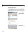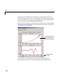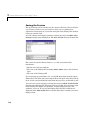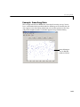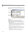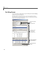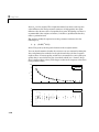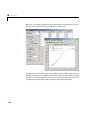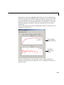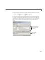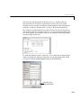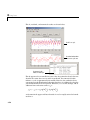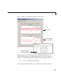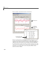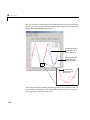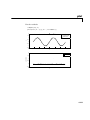
1
Curve Fitting Toolbox For Use with MATLAB ® Computation Visualization Programming User’s Guide Version 1 How to Contact The MathWorks: www.mathworks.com comp.soft-sys.matlab Web Newsgroup [email protected] Technical support Product enhancement suggestions Bug reports Documentation error reports Order status, license renewals, passcodes Sales, pricing, and general information 508-647-7000 Phone 508-647-7001 Fax The MathWorks, Inc. 3 Apple Hill Drive Natick, MA 01760-2098 Mail [email protected] [email protected] [email protected] [email protected] [email protected] For contact information about worldwide offices, see the MathWorks Web site. Curve Fitting Toolbox User’s Guide COPYRIGHT 2001-2002 by The MathWorks, Inc. The software described in this document is furnished under a license agreement. The software may be used or copied only under the terms of the license agreement. No part of this manual may be photocopied or reproduced in any form without prior written consent from The MathWorks, Inc. FEDERAL ACQUISITION: This provision applies to all acquisitions of the Program and Documentation by or for the federal government of the United States. By accepting delivery of the Program, the government hereby agrees that this software qualifies as "commercial" computer software within the meaning of FAR Part 12.212, DFARS Part 227.7202-1, DFARS Part 227.7202-3, DFARS Part 252.227-7013, and DFARS Part 252.227-7014. The terms and conditions of The MathWorks, Inc. Software License Agreement shall pertain to the government’s use and disclosure of the Program and Documentation, and shall supersede any conflicting contractual terms or conditions. If this license fails to meet the government’s minimum needs or is inconsistent in any respect with federal procurement law, the government agrees to return the Program and Documentation, unused, to MathWorks. MATLAB, Simulink, Stateflow, Handle Graphics, and Real-Time Workshop are registered trademarks, and TargetBox is a trademark of The MathWorks, Inc. Other product or brand names are trademarks or registered trademarks of their respective holders. Printing History: July 2001 July 2002 First printing Second printing New for Version 1 (Release 12.1) Revised for Version 1.1 (Release 13) Contents Preface What Is the Curve Fitting Toolbox? . . . . . . . . . . . . . . . . . . . . . . vi Exploring the Toolbox . . . . . . . . . . . . . . . . . . . . . . . . . . . . . . . . . . vi Related Products . . . . . . . . . . . . . . . . . . . . . . . . . . . . . . . . . . . . . viii Using This Guide . . . . . . . . . . . . . . . . . . . . . . . . . . . . . . . . . . . . . . ix Expected Background . . . . . . . . . . . . . . . . . . . . . . . . . . . . . . . . . . ix How This Guide Is Organized . . . . . . . . . . . . . . . . . . . . . . . . . . . . ix Documentation Examples and Data Sets . . . . . . . . . . . . . . . . . . . . x Installation Information . . . . . . . . . . . . . . . . . . . . . . . . . . . . . . . . xi Typographical Conventions . . . . . . . . . . . . . . . . . . . . . . . . . . . . . xii Getting Started with the Curve Fitting Toolbox 1 Opening the Curve Fitting Tool . . . . . . . . . . . . . . . . . . . . . . . . 1-2 Importing the Data . . . . . . . . . . . . . . . . . . . . . . . . . . . . . . . . . . . 1-3 Fitting the Data . . . . . . . . . . . . . . . . . . . . . . . . . . . . . . . . . . . . . . 1-5 The Data Fitting Procedure . . . . . . . . . . . . . . . . . . . . . . . . . . . . 1-5 Determining the Best Fit . . . . . . . . . . . . . . . . . . . . . . . . . . . . . . 1-8 Saving the Fit Results . . . . . . . . . . . . . . . . . . . . . . . . . . . . . . . . 1-13 Analyzing the Fit . . . . . . . . . . . . . . . . . . . . . . . . . . . . . . . . . . . . 1-15 Saving the Analysis Results . . . . . . . . . . . . . . . . . . . . . . . . . . . 1-16 i Saving Your Work . . . . . . . . . . . . . . . . . . . . . . . . . . . . . . . . . . . . 1-17 Saving the Session . . . . . . . . . . . . . . . . . . . . . . . . . . . . . . . . . . . 1-18 Generating an M-File . . . . . . . . . . . . . . . . . . . . . . . . . . . . . . . . 1-19 Importing, Viewing, and Preprocessing Data 2 Importing Data Sets . . . . . . . . . . . . . . . . . . . . . . . . . . . . . . . . . . . 2-2 Example: Importing Data . . . . . . . . . . . . . . . . . . . . . . . . . . . . . . 2-4 Viewing Data . . . . . . . . . . . . . . . . . . . . . . . . . . . . . . . . . . . . . . . . . 2-6 Viewing Data Graphically . . . . . . . . . . . . . . . . . . . . . . . . . . . . . . 2-6 Viewing Data Numerically . . . . . . . . . . . . . . . . . . . . . . . . . . . . . 2-8 Smoothing Data . . . . . . . . . . . . . . . . . . . . . . . . . . . . . . . . . . . . . . . 2-9 Moving Average Filtering . . . . . . . . . . . . . . . . . . . . . . . . . . . . . 2-12 Lowess and Loess: Local Regression Smoothing . . . . . . . . . . . 2-14 Savitzky-Golay Filtering . . . . . . . . . . . . . . . . . . . . . . . . . . . . . . 2-19 Example: Smoothing Data . . . . . . . . . . . . . . . . . . . . . . . . . . . . . 2-21 Excluding and Sectioning Data . . . . . . . . . . . . . . . . . . . . . . . . Marking Outliers . . . . . . . . . . . . . . . . . . . . . . . . . . . . . . . . . . . . Sectioning . . . . . . . . . . . . . . . . . . . . . . . . . . . . . . . . . . . . . . . . . . Example: Excluding and Sectioning Data . . . . . . . . . . . . . . . . Example: Sectioning Periodic Data . . . . . . . . . . . . . . . . . . . . . . 2-25 2-27 2-30 2-32 2-35 Additional Preprocessing Steps . . . . . . . . . . . . . . . . . . . . . . . 2-40 Transforming the Response Data . . . . . . . . . . . . . . . . . . . . . . . 2-40 Removing Infs, NaNs, and Outliers . . . . . . . . . . . . . . . . . . . . . 2-41 Selected Bibliography . . . . . . . . . . . . . . . . . . . . . . . . . . . . . . . . 2-42 ii Contents Fitting Data 3 The Fitting Process . . . . . . . . . . . . . . . . . . . . . . . . . . . . . . . . . . . 3-2 Parametric Fitting . . . . . . . . . . . . . . . . . . . . . . . . . . . . . . . . . . . . 3-4 Basic Assumptions About the Error . . . . . . . . . . . . . . . . . . . . . . 3-5 The Least Squares Fitting Method . . . . . . . . . . . . . . . . . . . . . . . 3-6 Library Models . . . . . . . . . . . . . . . . . . . . . . . . . . . . . . . . . . . . . . 3-16 Custom Equations . . . . . . . . . . . . . . . . . . . . . . . . . . . . . . . . . . . 3-20 Specifying Fit Options . . . . . . . . . . . . . . . . . . . . . . . . . . . . . . . . 3-23 Evaluating the Goodness of Fit . . . . . . . . . . . . . . . . . . . . . . . . . 3-27 Example: Rational Fit . . . . . . . . . . . . . . . . . . . . . . . . . . . . . . . . 3-41 Example: Fitting with Custom Equations . . . . . . . . . . . . . . . . 3-46 Example: Robust Fit . . . . . . . . . . . . . . . . . . . . . . . . . . . . . . . . . 3-61 Nonparametric Fitting . . . . . . . . . . . . . . . . . . . . . . . . . . . . . . . Interpolants . . . . . . . . . . . . . . . . . . . . . . . . . . . . . . . . . . . . . . . . Smoothing Spline . . . . . . . . . . . . . . . . . . . . . . . . . . . . . . . . . . . . Example: Nonparametric Fit . . . . . . . . . . . . . . . . . . . . . . . . . . . 3-68 3-68 3-70 3-72 Selected Bibliography . . . . . . . . . . . . . . . . . . . . . . . . . . . . . . . . 3-75 Function Reference 4 Functions – By Category . . . . . . . . . . . . . . . . . . . . . . . . . . . . . . Fitting Data . . . . . . . . . . . . . . . . . . . . . . . . . . . . . . . . . . . . . . . . Getting Information and Help . . . . . . . . . . . . . . . . . . . . . . . . . . Getting and Setting Properties . . . . . . . . . . . . . . . . . . . . . . . . . Preprocessing Data . . . . . . . . . . . . . . . . . . . . . . . . . . . . . . . . . . Postprocessing Data . . . . . . . . . . . . . . . . . . . . . . . . . . . . . . . . . . General Purpose . . . . . . . . . . . . . . . . . . . . . . . . . . . . . . . . . . . . . 4-78 4-78 4-78 4-78 4-78 4-79 4-79 Functions – Alphabetical List . . . . . . . . . . . . . . . . . . . . . . . . . 4-80 iii iv Contents Preface This chapter provides an overview of the Curve Fitting Toolbox, as well as information about this documentation. The sections are as follows. What Is the Curve Fitting Toolbox? (p. vi) The toolbox and the kinds of tasks it can perform Related Products (p. viii) MathWorks products related to this toolbox Using This Guide (p. ix) An overview of this guide Installation Information (p. xi) How to determine whether the toolbox is installed on your system Typographical Conventions Typographical conventions that this guide uses (p. xii) Preface What Is the Curve Fitting Toolbox? The Curve Fitting Toolbox is a collection of graphical user interfaces (GUIs) and M-file functions built on the MATLAB® technical computing environment. The toolbox provides you with these main features: • Data preprocessing such as sectioning and smoothing • Parametric and nonparametric data fitting: - You can perform a parametric fit using a toolbox library equation or using a custom equation. Library equations include polynomials, exponentials, rationals, sums of Gaussians, and so on. Custom equations are equations that you define to suit your specific curve fitting needs. - You can perform a nonparametric fit using a smoothing spline or various interpolants. • Standard linear least squares, nonlinear least squares, weighted least squares, constrained least squares, and robust fitting procedures • Fit statistics to assist you in determining the goodness of fit • Analysis capabilities such as extrapolation, differentiation, and integration • A graphical environment that allows you to: - Explore and analyze data sets and fits visually and numerically - Save your work in various formats including M-files, binary files, and workspace variables Exploring the Toolbox The Curve Fitting Toolbox consists of two different environments: a graphical user interface (GUI) environment and the usual MATLAB command line environment. Although the two environments are functionally equivalent, you generally cannot mix the two when performing a given curve fitting task. For example, you cannot generate a fit at the command line and then import that fit into the graphical environment. However, you can create a fit in the graphical environment and then generate an associated M-file. You can then recreate the fit from the command line and modify the M-file according to your needs. For this reason, as well as for the enhanced data analysis and exploration tools that are available, we recommend you use the graphical environment for most tasks. vi What Is the Curve Fitting Toolbox? You can explore the graphical environment by typing cftool Click the GUI Help buttons to learn how to proceed. Additionally, you can follow the examples in the tutorial sections of this guide, which are all GUI oriented. To explore the command line environment, you can list the toolbox functions by typing help curvefit To view the code for any function, type type function_name To view the help for any function, type help function_name You can change the way any toolbox function works by copying and renaming the M-file, and then modifying your copy. However, these changes will not be reflected in the graphical environment. You can also extend the toolbox by adding your own M-files, or by using it in combination with other products such as the Statistics Toolbox or the Optimization Toolbox. vii Preface Related Products The Curve Fitting Toolbox requires MATLAB 6.5 (Release 13). Additionally, The MathWorks provides several related products that are especially relevant to the kinds of tasks you can perform with the Curve Fitting Toolbox. For more information about any of these products, see either • The online documentation for that product if it is installed or if you are reading the documentation from the CD • The MathWorks Web site, at http://www.mathworks.com; see the “products” section Note The toolboxes listed below all include functions that extend the capabilities of MATLAB. viii Product Description Optimization Toolbox Solve standard and large-scale optimization problems Spline Toolbox Create and manipulate spline approximation models of data Statistics Toolbox Apply statistical algorithms and probability models Using This Guide Using This Guide Expected Background This guide assumes that you already have background knowledge in the subject of curve fitting data. If you do not yet have this background, then you should read a standard curve fitting text, some of which are listed in “Selected Bibliography” on page 3-75. When learning to use the toolbox, you should start with Chapter 1, “Getting Started with the Curve Fitting Toolbox,” which illustrates the major toolbox features by fitting census data to several equations and then evaluating the best fit. More detailed information about the features discussed in this chapter is available elsewhere in the guide, and you should browse the documentation according to your needs. How This Guide Is Organized The organization of this guide is described below. Chapter Description Getting Started with the Curve Fitting Toolbox Describes a particular example in detail to help you get started with the toolbox. Importing, Viewing, and Preprocessing Data Describes how to import, view, and smooth data sets, and how to exclude one or more data points in a data set from subsequent fits. Fitting Data Describes how to fit data using library or custom equations, a smoothing spline, or an interpolant. Several detailed examples are included as well. Function Reference Describes all toolbox functions in detail. ix Preface Documentation Examples and Data Sets To learn how to use the Curve Fitting Toolbox, you can follow the examples included in this guide. A quick way to locate these examples is with the example index, which you can access via the Help browser. Some examples use data that is generated as part of the example, while other examples use data sets that are included with the toolbox or with MATLAB. These data sets are stored as MAT-files and are listed below. Data Set Description carbon12alpha Generated data associated with the nuclear reaction 12 C(e,e’,α)8Be. The data set is based on the experiment described by reference [8] in Chapter 3, “Fitting Data.” census United States population figures for the years 1790 to 1990 in 10-year increments. The data set is included with MATLAB. enso Measured data of monthly averaged atmospheric pressure differences between Easter Island and Darwin, Australia. flvote2k 2000 U. S. presidential election results for the state of Florida. The data set was obtained from http://election.dos.state.fl.us/. gauss3 Generated data consisting of two poorly resolved Gaussian peaks on an exponential background. hahn1 Measured data of the thermal expansion of copper as a function of temperature. The enso, gauss3, and hahn1 data sets were obtained from the Statistical Reference Datasets collection, which is provided by the Information Technology Laboratory of the National Institute of Standards and Technology. The Web site is http://www.itl.nist.gov/div898/strd. x Installation Information Installation Information To determine if the Curve Fitting Toolbox is installed on your system, type ver at the MATLAB prompt. MATLAB displays information about the version of MATLAB you are running, including a list of installed add-on products and their version numbers. Check the list to see if the Curve Fitting Toolbox appears. For information about installing the toolbox, refer to the MATLAB Installation Guide for your platform. If you experience installation difficulties and have Web access, look for the installation and license information at the MathWorks Web site http://www.mathworks.com/support. xi Preface Typographical Conventions This guide uses some or all of these conventions. Item Convention Example Example code Monospace font To assign the value 5 to A, enter A = 5 Function names, syntax, filenames, directory/folder names, and user input Monospace font The cos function finds the cosine of each array element. Syntax line example is MLGetVar ML_var_name Buttons and keys Boldface with book title caps Press the Enter key. Literal strings (in syntax descriptions in reference chapters) Monospace bold for literals f = freqspace(n,'whole') Italics for variables This vector represents the polynomial p = x2 + 2x + 3. Mathematical expressions MATLAB output Standard text font for functions, operators, and constants Monospace font MATLAB responds with A = 5 xii Menu and dialog box titles Boldface with book title caps Choose the File Options menu. New terms and for emphasis Italics An array is an ordered collection of information. Omitted input arguments (...) ellipsis denotes all of the input/output arguments from preceding syntaxes. [c,ia,ib] = union(...) String variables (from a finite list) Monospace italics sysc = d2c(sysd,'method') 1 Getting Started with the Curve Fitting Toolbox This chapter describes a particular example in detail to help you get started with the Curve Fitting Toolbox. In this example, you will fit census data to several toolbox library models, find the best fit, and extrapolate the best fit to predict the US population in future years. In doing so, the basic steps involved in any curve fitting scenario are illustrated. These steps include Opening the Curve Fitting Tool (p. 1-2) The Curve Fitting Tool is the main toolbox interface. Importing the Data (p. 1-3) The data must exist as vectors in the MATLAB workspace. After importing, you can view the data, mark data points to be excluded from the fit, and smooth the data. Fitting the Data (p. 1-5) Explore various parametric and nonparametric fits, and compare fit results graphically and numerically. Analyzing the Fit (p. 1-15) Evaluate (interpolate or extrapolate), differentiate, or integrate the fit. Saving Your Work (p. 1-17) Save your work for documentation purposes or for later analysis. 1 Getting Started with the Curve Fitting Toolbox Opening the Curve Fitting Tool The Curve Fitting Tool is a graphical user interface (GUI) that allows you to • Visually explore one or more data sets and fits as scatter plots. • Graphically evaluate the goodness of fit using residuals and prediction bounds. • Access additional interfaces for - Importing, viewing, and smoothing data - Fitting data, and comparing fits and data sets - Marking data points to be excluded from a fit - Selecting which fits and data sets are displayed in the tool - Interpolating, extrapolating, differentiating, or integrating fits You open the Curve Fitting Tool with the cftool command. cftool 1-2 Importing the Data Importing the Data Before you can import data into the Curve Fitting Tool, the data variables must exist in the MATLAB workspace. For this example, the data is stored in the file census.mat, which is provided with MATLAB. load census The workspace now contains two new variables, cdate and pop: • cdate is a column vector containing the years 1790 to 1990 in 10-year increments. • pop is a column vector with the US population figures that correspond to the years in cdate. You can import data into the Curve Fitting Tool with the Data GUI. You open this GUI by clicking the Data button on the Curve Fitting Tool. As shown below, the Data GUI consists of two panes: Data sets and Smooth. The Data Sets pane allows you to • Import predictor (X) data, response (Y) data, and weights. If you do not import weights, then they are assumed to be 1 for all data points. • Specify the name of the data set. • Preview the data. 1-3 1 Getting Started with the Curve Fitting Toolbox To load cdate and pop into the Curve Fitting Tool, select the appropriate variable names from the X Data and Y Data lists. The data is then displayed in the Preview window. Click the Create data set button to complete the data import process. Select the data variable names. Click Create data set to import the data. The Smooth pane is described in Chapter 2, “Importing, Viewing, and Preprocessing Data.” 1-4 Fitting the Data Fitting the Data You fit data with the Fitting GUI. You open this GUI by clicking the Fitting button on the Curve Fitting Tool. The Fitting GUI consists of two parts: the Fit Editor and the Table of Fits. The Fit Editor allows you to • Specify the fit name, the current data set, and the exclusion rule. • Explore various fits to the current data set using a library or custom equation, a smoothing spline, or an interpolant. • Override the default fit options such as the coefficient starting values. • Compare fit results including the fitted coefficients and goodness of fit statistics. The Table of Fits allows you to • Keep track of all the fits and their data sets for the current session. • Display a summary of the fit results. • Save or delete the fit results. The Data Fitting Procedure For this example, begin by fitting the census data with a second degree polynomial. Then continue fitting the data using polynomial equations up to sixth degree, and a single-term exponential equation. The data fitting procedure follows these general steps: 1 From the Fit Editor, click New Fit. Note that this action always defaults to a linear polynomial fit type. You use New Fit at the beginning of your curve fitting session, and when you are exploring different fit types for a given data set. 2 Because the initial fit uses a second degree polynomial, select quadratic polynomial from the Polynomial list. Name the fit poly2. 3 Click the Apply button or select the Immediate apply check box. The library model, fitted coefficients, and goodness of fit statistics are displayed in the Results area. 1-5 1 Getting Started with the Curve Fitting Toolbox 4 Fit the additional library equations. For fits of a given type (for example, polynomials), you should use Copy Fit instead of New Fit because copying a fit retains the current fit type state thereby requiring fewer steps than creating a new fit each time. The Fitting GUI is shown below with the results of fitting the census data with a quadratic polynomial. The Fit Editor allows you to select a data set and a fit name, and to explore and compare various library and custom fits. The Table of Fits allows you to keep track of all the fits, their data sets, and fit results for the current session. 1-6 Fitting the Data The data, fit, and residuals are shown below. You display the residuals as a line plot by selecting the menu item View->Residuals->Line plot from the Curve Fitting Tool. These residuals indicate that a better fit may be possible. The residuals indicate that a better fit may be possible. Therefore, you should continue fitting the census data following the procedure outlined in the beginning of this section. The residuals from a good fit should look random with no apparent pattern. A pattern, such as a tendency for consecutive residuals to have the same sign, can be an indication that a better model exists. 1-7 1 Getting Started with the Curve Fitting Toolbox When you fit higher degree polynomials, the Results area displays this warning: Equation is badly conditioned. Remove repeated data points or try centering and scaling. The warning arises because the fitting procedure uses the cdate values as the basis for a matrix with very large values. The spread of the cdate values results in scaling problems. To address this problem, you can normalize the cdate data. Normalization is a process of scaling the predictor data to improve the accuracy of the subsequent numeric computations. A way to normalize cdate is to center it at zero mean and scale it to unit standard deviation. (cdate - mean(cdate))./std(cdate) To normalize data with the Curve Fitting Tool, select the Center and scale X data check box. Note Because the predictor data changes after normalizing, the values of the fitted coefficients also change when compared to the original data. However, the functional form of the data and the resulting goodness of fit statistics do not change. Additionally, the data is displayed in the Curve Fitting Tool using the original scale. Determining the Best Fit To determine the best fit, you should examine both the graphical and numerical fit results. Examining the Graphical Fit Results Your initial approach in determining the best fit should be a graphical examination of the fits and residuals. The graphical fit results shown below indicate that • The fits and residuals for the polynomial equations are all similar, making it difficult to choose the best one. 1-8 Fitting the Data • The fit and residuals for the single-term exponential equation indicate it is a poor fit overall. Therefore, it is a poor choice for extrapolation. To easily view all the data, fits, and residuals, turn the legend off. The residuals for the polynomial fits are all similar making it difficult to choose the best one. The residuals for the exponential fit indicate it is a poor fit overall. Use the Plotting GUI to remove exp1 from the scatter plot display. Remove this fit from the scatter plot. 1-9 1 Getting Started with the Curve Fitting Toolbox Because the goal of fitting the census data is to extrapolate the best fit to predict future population values, you should explore the behavior of the fits up to the year 2050. You can change the axes limits of the Curve Fitting Tool by selecting the menu item Tools->Axes Limit Control. The census data and fits are shown below for an upper abscissa limit of 2050. The behavior of the sixth degree polynomial fit beyond the data range makes it a poor choice for extrapolation. The sixth degree polynomial fit beyond the data range makes it a poor choice for extrapolation. Change the upper abscissa limit to 2050. As you can see, you should exercise caution when extrapolating with polynomial fits because they can diverge wildly outside the data range. 1-10 Fitting the Data Examining the Numerical Fit Results Because you can no longer eliminate fits by examining them graphically, you should examine the numerical fit results. There are two types of numerical fit results displayed in the Fitting GUI: goodness of fit statistics and confidence intervals on the fitted coefficients. The goodness of fit statistics help you determine how well the curve fits the data. The confidence intervals on the coefficients determine their accuracy. Some goodness of fit statistics are displayed in the Results area of the Fit Editor for a single fit. All goodness of fit statistics are displayed in the Table of Fits for all fits, which allows for easy comparison. In this example, the sum of squares due to error (SSE) and the adjusted R-square statistics are used to help determine the best fit. As described in “Goodness of Fit Statistics” on page 3-29, the SSE statistic is the least squares error of the fit, with a value closer to zero indicating a better fit. The adjusted R-square statistic is generally the best indicator of the fit quality when you add additional coefficients to your model. You can modify the information displayed in the Table of Fits with the Table Options GUI. You open this GUI by clicking the Table options button on the Fitting GUI. As shown below, select the adjusted R-square statistic and clear the R-square statistic. Do not display the R-square statistic in the Table of Fits. Display the adjusted R-square statistic in the Table of Fits. 1-11 1 Getting Started with the Curve Fitting Toolbox The numerical fit results are shown below. You can click the Table of Fits column headings to sort by statistics results. The SSE for exp1 indicates it is a poor fit, which was already determined by examining the fit and residuals. The lowest SSE value is associated with poly6. However, the behavior of this fit beyond the data range makes it a poor choice for extrapolation. The next best SSE value is associated with the fifth degree polynomial fit, poly5, suggesting it may be the best fit. However, the SSE and adjusted R-square values for the remaining polynomial fits are all very close to each other. Which one should you choose? The confidence bounds for the p1-p3 coefficients suggest that a fifth degree polynomial overfits the census data. Click this column heading to sort the fits by the SSE values. The SSE and adjusted R-square values suggest that the fifth degree polynomial fit is the best one. 1-12 Fitting the Data To resolve this issue, examine the confidence bounds for the remaining fits. By default, 95% confidence bounds are calculated. You can change this level by selecting the menu item View->Confidence Level from the Curve Fitting Tool. The p1, p2, and p3 coefficients for the fifth degree polynomial suggest that it overfits the census data. However, the confidence bounds for the quadratic fit, poly2, indicate that the fitted coefficients are known fairly accurately. Therefore, after examining both the graphical and numerical fit results, it appears that you should use poly2 to extrapolate the census data. Note The fitted coefficients associated with the constant, linear, and quadratic terms are nearly identical for each polynomial equation. However, as the polynomial degree increases, the coefficient bounds associated with the higher degree terms increase, which suggests overfitting. For more information about confidence bounds, refer to “Confidence and Prediction Bounds” on page 3-32. Saving the Fit Results By clicking the Save to workspace button, you can save the selected fit and the associated fit results to the MATLAB workspace. The fit is saved as a MATLAB object and the associated fit results are saved as structures. This example saves all the fit results for the best fit, poly2. fittedmodel1 is saved as a Curve Fitting Toolbox cfit object. whos fittedmodel1 Name fittedmodel1 Size 1x1 Bytes 6178 Class cfit object Grand total is 386 elements using 6178 bytes 1-13 1 Getting Started with the Curve Fitting Toolbox The cfit object display includes the model, the fitted coefficients, and the confidence bounds for the fitted coefficients. fittedmodel1 fittedmodel1 = Linear model Poly2: fittedmodel1(x) = p1*x^2 + p2*x + p3 Coefficients (with 95% confidence bounds): p1 = 0.006541 (0.006124, 0.006958) p2 = -23.51 (-25.09, -21.93) p3 = 2.113e+004 (1.964e+004, 2.262e+004) The goodness1 structure contains goodness of fit results. goodness1 goodness1 = sse: rsquare: dfe: adjrsquare: rmse: 159.0293 0.9987 18 0.9986 2.9724 The output1 structure contains additional information associated with the fit. output1 output1 = numobs: numparam: residuals: Jacobian: exitflag: algorithm: 1-14 21 3 [21x1 double] [21x3 double] 1 'QR factorization and solve' Analyzing the Fit Analyzing the Fit You can evaluate (interpolate or extrapolate), differentiate, or integrate a fit over a specified data range with the Analysis GUI. You open this GUI by clicking the Analysis button on the Curve Fitting Tool. For this example, you will extrapolate the quadratic polynomial fit to predict the US population from the year 2000 to the year 2050 in 10 year increments, and then plot both the analysis results and the data. To do this: • Enter the appropriate MATLAB vector in the Analyze at Xi field. • Select the Evaluate fit at Xi check box. • Select the Plot results and Plot data set check boxes. • Click the Apply button. The numerical extrapolation results are shown below. Specify the fit and data to analyze. Select this check box to extrapolate. Plot both the analysis results and the data. 1-15 1 Getting Started with the Curve Fitting Toolbox The extrapolated values and the census data set are displayed together in a new figure window. Saving the Analysis Results By clicking the Save to workspace button, you can save the extrapolated values as a structure to the MATLAB workspace. The resulting structure is shown below. analysisresults1 analysisresults1 = xi: [6x1 double] yfit: [6x1 double] 1-16 Saving Your Work Saving Your Work The Curve Fitting Toolbox provides you with several options for saving your work. For example, as described in “Saving the Fit Results” on page 1-13, you can save one or more fits and the associated fit results as variables to the MATLAB workspace. You can then use this saved information for documentation purposes, or to extend your data exploration and analysis. In addition to saving your work to MATLAB workspace variables, you can • Save the session. • Generate an M-file. Before performing any of these tasks, you may want to remove unwanted data sets and fits from the Curve Fitting Tool display. An easy way to do this is with the Plotting GUI. The Plotting GUI shown below is configured to display only the census data and the best fit, poly2. Clear the remaining fits associated with the census data except the best fit. 1-17 1 Getting Started with the Curve Fitting Toolbox Saving the Session The curve fitting session is defined as the current collection of fits for all data sets. You may want to save your session so that you can continue data exploration and analysis at a later time using the Curve Fitting Tool without losing any current work. Save the current curve fitting session by selecting the menu item File->Save Session from the Curve Fitting Tool. The Save Session dialog is shown below. The session is stored in binary form in a cfit file, and contains this information: • All data sets and associated fits • The state of the Fitting GUI, including Table of Fits entries and exclusion rules • The state of the Plotting GUI To avoid saving unwanted data sets, you should delete them from the Curve Fitting Tool. You delete data sets using the Data Sets pane of the Data GUI. If there are fits associated with the unwanted data sets, they are deleted as well. You can load a saved session by selecting the menu item File->Load Session from the Curve Fitting Tool. When the session is loaded, the saved state of the Curve Fitting Tool display is reproduced, and may display the data, fits, residuals, and so on. If you open the Fitting GUI, then the loaded fits are displayed in the Table of Fits. Select a fit from this table to continue your curve fitting session. 1-18 Saving Your Work Generating an M-File You may want to generate an M-file so that you can continue data exploration and analysis from the MATLAB command line. You can run the M-file without modification to recreate the fits and results that you created with the Curve Fitting Tool, or you can edit and modify the file as needed. For detailed descriptions of the functions provided by the toolbox, refer to Chapter 4, “Function Reference.” If you have many data sets to fit and you want to automate the fitting process, you should use the Curve Fitting Tool to select the appropriate model and fit options, generate an M-file, and then run the M-file in batch mode. Save your work to an M-file by selecting the menu item File->Save M-file from the Curve Fitting Tool. The Save M-File dialog is shown below. The M-file can capture this information from the Curve Fitting Tool: • All data set variable names, associated fits, and residuals • Fit options such as whether the data should be normalized, the fit starting points, and the fitting method You can recreate the saved fits in a new figure window by typing the name of the M-file at the MATLAB command line. Note that you must provide the appropriate data variables as inputs to the M-file. These variables are given in the M-file help. 1-19 1 Getting Started with the Curve Fitting Toolbox For example, the help for the censusfit M-file indicates that the variables cdate and pop are required to recreate the saved fit. help censusfit CENSUSFIT Create plot of datasets and fits CENSUSFIT(CDATE,POP) Creates a plot, similar to the plot in the main curve fitting window, using the data that you provide as input. You can apply this function to the same data you used with cftool or with different data. You may want to edit the function to customize the code and this help message. Number of datasets: Number of fits: 6 1-20 1 2 Importing, Viewing, and Preprocessing Data This chapter describes how to import, view, and preprocess data with the Curve Fitting Toolbox. You import data with the Data GUI, and view data graphically as a scatter plot using the Curve Fitting Tool. The main preprocessing steps are smoothing, and excluding and sectioning data. You smooth data with the Data GUI, and exclude and section data with the Exclude GUI. The sections are as follows. Importing Data Sets (p. 2-2) Select workspace variables that compose the data set, list all imported and generated data sets, and delete one or more data sets. Viewing Data (p. 2-6) View the data graphically as a scatter plot. Smoothing Data (p. 2-9) Reduce noise in a data set using moving average filtering, lowess or robust lowess, loess or robust loess, or Savitzky-Golay filtering. Excluding and Sectioning Data (p. 2-25) Mark individual data points (outliers) to be excluded from a fit, or mark a range of data points (sectioning) to be excluded from a fit. Additional Preprocessing Steps (p. 2-40) Additional preprocessing steps not available through the Data GUI, such as transforming the response data and removing Infs, NaNs, and outliers from a data set. Selected Bibliography (p. 2-42) Resources for additional information. 2 Importing, Viewing, and Preprocessing Data Importing Data Sets You import data sets into the Curve Fitting Tool with the Data Sets pane of the Data GUI. Using this pane, you can • Select workspace variables that compose a data set • Display a list of all imported data sets • View, delete, or rename one or more data sets The Data Sets pane is shown below followed by a description of its features. Construct and name the data set. Data sets list 2-2 Importing Data Sets Construct and Name the Data Set • Import workspace vectors — All selected variables must be the same length. You can import only vectors, not matrices or scalars. Infs and NaNs are ignored because you cannot fit data containing these values, and only the real part of a complex number is used. To perform any curve-fitting task, you must select at least one vector of data: - X data — Select the predictor data. - Y data — Select the response data. - Weights — Select the weights associated with the response data. If weights are not imported, they are assumed to be 1 for all data points. • Preview — The selected workspace vectors are displayed graphically in the preview window. Weights are not displayed. • Data set name — The name of the imported data set. The toolbox automatically creates a unique name for each imported data set. You can change the name by editing this field. Click the Create data set button to complete the data import process. Data Sets List • Data sets — Lists all data sets added to the Curve Fitting Tool. The data sets can be created from workspace variables, or from smoothing an existing imported data set. When you select a data set, you can perform these actions: - Click View to open the View Data Set GUI. Using this GUI, you can view a single data set both graphically and numerically. Additionally, you can display data points to be excluded in a fit by selecting an exclusion rule. - Click Rename to change the name of a single data set. - Click Delete to delete one or more data sets. To select multiple data sets, you can use the Ctrl key and the mouse to select data sets one by one, or you can use the Shift key and the mouse to select a range of data sets. 2-3 2 Importing, Viewing, and Preprocessing Data Example: Importing Data This example imports the ENSO data set into the Curve Fitting Toolbox using the Data Sets pane of the Data GUI. The first step is to load the data from the file enso.mat into the MATLAB workspace. load enso The workspace contains two new variables, pressure and month: • pressure is the monthly averaged atmospheric pressure differences between Easter Island and Darwin, Australia. This difference drives the trade winds in the southern hemisphere. • month is the relative time in months. Alternatively, you can import data by specifying the variable names as arguments to the cftool function. cftool(month,pressure) In this case, the Data GUI is not opened. Data Import Process The data import process is described below: 1 Select workspace variables. The predictor and response data are displayed graphically in the Preview window. Weights and data points containing Infs or NaNs are not displayed. 2 Specify the data set name. You should specify a meaningful name when you import multiple data sets. If you do not specify a name, the default name, which is constructed from the selected variable names, is used. 2-4 Importing Data Sets 3 Click the Create data set button. The Data sets list box displays all the data sets added to the toolbox. Note that you can construct data sets from workspace variables, or by smoothing an existing data set. If your data contains Infs or complex values, a warning message such as the message shown below is displayed. The Data Sets pane shown below displays the imported ENSO data in the Preview window. After you click the Create data set button, the data set enso is added to the Data sets list box. You can then view, rename, or delete enso by selecting it in the list box and clicking the appropriate button. Select the workspace variable names. Specify the data set name. Click Create data set to import the data. 2-5 2 Importing, Viewing, and Preprocessing Data Viewing Data The Curve Fitting Toolbox provides two ways to view imported data: • Graphically in a scatter plot • Numerically in a table Viewing Data Graphically After you import a data set, it is automatically displayed as a scatter plot in the Curve Fitting Tool. The response data is plotted on the vertical axis and the predictor data is plotted on the horizontal axis. The scatter plot is a powerful tool because it allows you to view the entire data set at once, and it can easily display a wide range of relationships between the two variables. You should examine the data carefully to determine whether preprocessing is required, or to deduce a reasonable fitting approach. For example, it’s typically very easy to identify outliers in a scatter plot, and to determine whether you should fit the data with a straight line, a periodic function, a sum of Gaussians, and so on. Enhancing the Graphical Display The Curve Fitting Toolbox provides several tools for enhancing the graphical display of a data set. These tools are available through the Tools menu, the GUI toolbar, and right-click menus. You can zoom in, zoom out, display data and fit tips, and so on using the Tools menu and the GUI toolbar shown below. GUI toolbar Tools menu 2-6 Viewing Data You can change the color, line width, line style, and marker type of the displayed data points using the right-click menu shown below. You activate this menu by placing your mouse over a data point and right-clicking. Note that a similar menu is available for fitted curves. Right-click menu The ENSO data is shown below after the display has been enhanced using several of these tools. Display the legend for the ENSO data set. Display data tips for the maximum response value. Change the color, marker type and line style for the data. Display the grid. Change the axis limits. 2-7 2 Importing, Viewing, and Preprocessing Data Viewing Data Numerically You can view the numerical values of a data set, as well as data points to be excluded from subsequent fits, with the View Data Set GUI. You open this GUI by selecting a name in the Data sets list box of the Data GUI and clicking the View button. The View Data Set GUI for the ENSO data set is shown below, followed by a description of its features. • Data set — Lists the names of the viewed data set and the associated variables. The data is displayed graphically below this list. The index, predictor data (X), response data (Y), and weights (if imported) are displayed numerically in the table. If the data contains Infs or NaNs, those values are labeled “ignored.” If the data contains complex numbers, only the real part is displayed. • Exclusion rules — Lists all the exclusion rules that are compatible with the viewed data set. When you select an exclusion rule, the data points marked for exclusion are grayed in the table, and are identified with an “x” in the graphical display. To exclude the data points while fitting, you must select the exclusion rule in the Fitting GUI. An exclusion rule is compatible with the viewed data set if their lengths are the same, or if it is created by sectioning only. 2-8 Smoothing Data Smoothing Data If your data is noisy, you might need to apply a smoothing algorithm to expose its features, and to provide a reasonable starting approach for parametric fitting. The two basic assumptions that underlie smoothing are • The relationship between the response data and the predictor data is smooth. • The smoothing process results in a smoothed value that is a better estimate of the original value because the noise has been reduced. The smoothing process attempts to estimate the average of the distribution of each response value. The estimation is based on a specified number of neighboring response values. You can think of smoothing as a local fit because a new response value is created for each original response value. Therefore, smoothing is similar to some of the nonparametric fit types supported by the toolbox, such as smoothing spline and cubic interpolation. However, this type of fitting is not the same as parametric fitting, which results in a global parameterization of the data. Note You should not fit data with a parametric model after smoothing, because the act of smoothing invalidates the assumption that the errors are normally distributed. Instead, you should consider smoothing to be a data exploration technique. There are two common types of smoothing methods: filtering (averaging) and local regression. Each smoothing method requires a span. The span defines a window of neighboring points to include in the smoothing calculation for each data point. This window moves across the data set as the smoothed response value is calculated for each predictor value. A large span increases the smoothness but decreases the resolution of the smoothed data set, while a small span decreases the smoothness but increases the resolution of the smoothed data set. The optimal span value depends on your data set and the smoothing method, and usually requires some experimentation to find. 2-9 2 Importing, Viewing, and Preprocessing Data The Curve Fitting Toolbox supports these smoothing methods: • Moving average filtering — Lowpass filter that takes the average of neighboring data points. • Lowess and loess — Locally weighted scatter plot smooth. These methods use linear least squares fitting, and a first-degree polynomial (lowess) or a second-degree polynomial (loess). Robust lowess and loess methods that are resistant to outliers are also available. • Savitzky-Golay filtering — A generalized moving average where you derive the filter coefficients by performing an unweighted linear least squares fit using a polynomial of the specified degree. Note that you can also smooth data using a smoothing spline. Refer to “Nonparametric Fitting” on page 3-68 for more information. You smooth data with the Smooth pane of the Data GUI. The pane is shown below followed by a description of its features. Data sets Smoothing method and parameters Data sets list 2-10 Smoothing Data Data Sets • Original data set — Select the data set you want to smooth. • Smoothed data set — Specify the name of the smoothed data set. Note that the process of smoothing the original data set always produces a new data set containing smoothed response values. Smoothing Method and Parameters • Method — Select the smoothing method. Each response value is replaced with a smoothed value that is calculated by the specified smoothing method. - Moving average — Filter the data by calculating an average. - Lowess — Locally weighted scatter plot smooth using linear least squares fitting and a first-degree polynomial. - Loess — Locally weighted scatter plot smooth using linear least squares fitting and a second-degree polynomial. - Savitzky-Golay — Filter the data with an unweighted linear least squares fit using a polynomial of the specified degree. - Robust Lowess — Lowess method that is resistant to outliers. - Robust Loess — Loess method that is resistant to outliers. • Span — The number of data points used to compute each smoothed value. For the moving average and Savitzky-Golay methods, the span must be odd. For all locally weighted smoothing methods, if the span is less than 1, it is interpreted as the percentage of the total number of data points. • Degree — The degree of the polynomial used in the Savitzky-Golay method. The degree must be smaller than the span. Data Sets List • Smoothed data sets — Lists all the smoothed data sets. You add a smoothed data set to the list by clicking the Create smoothed data set button. When you select a data set from the list, you can perform these actions: - Click View to open the View Data Set GUI. Using this GUI, you can view a single data set both graphically and numerically. Additionally, you can display data points to be excluded in a fit by selecting an exclusion rule. - Click Rename to change the name of a single data set. 2-11 2 Importing, Viewing, and Preprocessing Data - Click Delete to delete one or more data sets. To select multiple data sets, you can use the Ctrl key and the mouse to select data sets one by one, or you can use the Shift key and the mouse to select a range of data sets. - Click Save to workspace to save a single data set to a structure. Moving Average Filtering A moving average filter smooths data by replacing each data point with the average of the neighboring data points defined within the span. This process is equivalent to lowpass filtering with the response of the smoothing given by the difference equation 1 y s ( i ) = ------------------ ( y ( i + N ) + y ( i + N – 1 ) + … + y ( i – N ) ) 2N + 1 where ys(i) is the smoothed value for the ith data point, N is the number of neighboring data points on either side of ys(i), and 2N+1 is the span. The moving average smoothing method used by the Curve Fitting Toolbox follows these rules: • The span must be odd. • The data point to be smoothed must be at the center of the span. • The span is adjusted for data points that cannot accommodate the specified number of neighbors on either side. • The end points are not smoothed because a span cannot be defined. Note that you can use MATLAB’s filter function to implement difference equations such as the one shown above. However, because of the way that the end points are treated, the toolbox moving average result will differ from the result returned by filter. Refer to “Difference Equations and Filtering” in the MATLAB documentation for more information. For example, suppose you smooth data using a moving average filter with a span of 5. Using the rules described above, the first four elements of ys are given by ys(1) ys(2) ys(3) ys(4) 2-12 = = = = y(1) (y(1)+y(2)+y(3))/3 (y(1)+y(2)+y(3)+y(4)+y(5))/5 (y(2)+y(3)+y(4)+y(5)+y(6))/5 Smoothing Data Note that ys(1), ys(2), ... ,ys(end) refer to the order of the data after sorting, and not necessarily the original order. The smoothed values and spans for the first four data points of a generated data set are shown below. Moving Average Smoothing 80 80 Data Smoothed value Data Smoothed value 60 60 40 40 20 20 0 0 2 4 6 8 0 0 2 4 (a) 80 8 6 8 80 Data Smoothed value Data Smoothed value 60 60 40 40 20 20 0 6 (b) 0 2 4 6 (c) 8 0 0 2 4 (d) Plot (a) indicates that the first data point is not smoothed because a span cannot be constructed. Plot (b) indicates that the second data point is smoothed using a span of three. Plots (c) and (d) indicate that a span of five is used to calculate the smoothed value. 2-13 2 Importing, Viewing, and Preprocessing Data Lowess and Loess: Local Regression Smoothing The names “lowess” and “loess” are derived from the term “locally weighted scatter plot smooth,” as both methods use locally weighted linear regression to smooth data. The smoothing process is considered local because, like the moving average method, each smoothed value is determined by neighboring data points defined within the span. The process is weighted because a regression weight function is defined for the data points contained within the span. In addition to the regression weight function, you can use a robust weight function, which makes the process resistant to outliers. Finally, the methods are differentiated by the model used in the regression: lowess uses a linear polynomial, while loess uses a quadratic polynomial. The local regression smoothing methods used by the Curve Fitting Toolbox follow these rules: • The span can be even or odd. • You can specify the span as a percentage of the total number of data points in the data set. For example, a span of 0.1 uses 10% of the data points. The regression smoothing and robust smoothing procedures are described in detail below. Local Regression Smoothing Procedure The local regression smoothing process follows these steps for each data point: 1 Compute the regression weights for each data point in the span. The weights are given by the tricube function shown below. x–x 3 3 w i = 1 – -------------i d(x ) x is the predictor value associated with the response value to be smoothed, xi are the nearest neighbors of x as defined by the span, and d(x) is the distance along the abscissa from x to the most distant predictor value within the span. The weights have these characteristics: - The data point to be smoothed has the largest weight and the most influence on the fit. - Data points outside the span have zero weight and no influence on the fit. 2-14 Smoothing Data 2 A weighted linear least squares regression is performed. For lowess, the regression uses a first degree polynomial. For loess, the regression uses a second degree polynomial. 3 The smoothed value is given by the weighted regression at the predictor value of interest. If the smooth calculation involves the same number of neighboring data points on either side of the smoothed data point, the weight function is symmetric. However, if the number of neighboring points is not symmetric about the smoothed data point, then the weight function is not symmetric. Note that unlike the moving average smoothing process, the span never changes. For example, when you smooth the data point with the smallest predictor value, the shape of the weight function is truncated by one half, the leftmost data point in the span has the largest weight, and all the neighboring points are to the right of the smoothed value. The weight function for an end point and for an interior point is shown below for a span of 31 data points. Local Regression Weight Function 1.2 1 The weight function for the leftmost data point 0.8 0.6 0.4 0.2 0 0 20 40 60 80 100 60 80 100 1.2 1 The weight function for an interior data point 0.8 0.6 0.4 0.2 0 0 20 40 2-15 2 Importing, Viewing, and Preprocessing Data Using the lowess method with a span of five, the smoothed values and associated regressions for the first four data points of a generated data set are shown below. Lowess Smoothing 80 80 Data Smoothed value Data Smoothed value 60 60 40 40 20 20 0 0 2 4 6 8 0 0 2 4 (a) 80 8 6 8 80 Data Smoothed value Data Smoothed value 60 60 40 40 20 20 0 6 (b) 0 2 4 6 (c) 8 0 0 2 4 (d) Notice that the span does not change as the smoothing process progresses from data point to data point. However, depending on the number of nearest neighbors, the regression weight function might not be symmetric about the data point to be smoothed. In particular, plots (a) and (b) use an asymmetric weight function, while plots (c) and (d) use a symmetric weight function. For the loess method, the graphs would look the same except the smoothed value would be generated by a second-degree polynomial. 2-16 Smoothing Data Robust Smoothing Procedure If your data contains outliers, the smoothed values can become distorted, and not reflect the behavior of the bulk of the neighboring data points. To overcome this problem, you can smooth the data using a robust procedure that is not influenced by a small fraction of outliers. For a description of outliers, refer to “Marking Outliers” on page 2-27. The Curve Fitting Toolbox provides a robust version for both the lowess and loess smoothing methods. These robust methods include an additional calculation of robust weights, which is resistant to outliers. The robust smoothing procedure follows these steps: 1 Calculate the residuals from the smoothing procedure described in the previous section. 2 Compute the robust weights for each data point in the span. The weights are given by the bisquare function shown below. ( 1 – ( r i ⁄ 6MAD ) 2 ) wi = 0 2 r i < 6MAD r i ≥ 6MAD ri is the residual of the ith data point produced by the regression smoothing procedure, and MAD is the median absolute deviation of the residuals: MAD = median ( r ) The median absolute deviation is a measure of how spread out the residuals are. If ri is small compared to 6MAD, then the robust weight is close to 1. If ri is greater than 6MAD, the robust weight is 0 and the associated data point is excluded from the smooth calculation. 3 Smooth the data again using the robust weights. The final smoothed value is calculated using both the local regression weight and the robust weight. 4 Repeat the previous two steps for a total of five iterations. 2-17 2 Importing, Viewing, and Preprocessing Data The smoothing results of the lowess procedure are compared below to the results of the robust lowess procedure for a generated data set that contains a single outlier. The span for both procedures is 11 data points. Robust Lowess Smoothing 10 data lowess 5 0 0 1 2 3 4 5 6 (a) 5 residuals 0 −5 0 1 2 3 4 5 6 (b) 10 data robust lowess 5 0 0 1 2 3 4 5 6 (c) Plot (a) shows that the outlier influences the smoothed value for several nearest neighbors. Plot (b) suggests that the residual of the outlier is greater than six median absolute deviations. Therefore, the robust weight is zero for this data point. Plot (c) shows that the smoothed values neighboring the outlier reflect the bulk of the data. 2-18 Smoothing Data Savitzky-Golay Filtering Savitzky-Golay filtering can be thought of as a generalized moving average. You derive the filter coefficients by performing an unweighted linear least squares fit using a polynomial of a given degree. For this reason, a Savitzky-Golay filter is also called a digital smoothing polynomial filter or a least squares smoothing filter. Note that a higher degree polynomial makes it possible to achieve a high level of smoothing without attenuation of data features. The Savitzky-Golay filtering method is often used with frequency data or with spectroscopic (peak) data. For frequency data, the method is effective at preserving the high-frequency components of the signal. For spectroscopic data, the method is effective at preserving higher moments of the peak such as the line width. By comparison, the moving average filter tends to filter out a significant portion of the signal’s high-frequency content, and it can only preserve the lower moments of a peak such as the centroid. However, Savitzky-Golay filtering can be less successful than a moving average filter at rejecting noise. The Savitzky-Golay smoothing method used by the Curve Fitting Toolbox follows these rules: • The span must be odd. • The polynomial degree must be less than the span. • The data points are not required to have uniform spacing. Normally, Savitzky-Golay filtering requires uniform spacing of the predictor data. However, the algorithm provided by the Curve Fitting Toolbox supports nonuniform spacing. Therefore, you are not required to perform an additional filtering step to create data with uniform spacing. The plot shown below displays generated Gaussian data and several attempts at smoothing using the Savitzky-Golay method. The data is very noisy and the peak widths vary from broad to narrow. The span is equal to 5% of the number of data points. 2-19 2 Importing, Viewing, and Preprocessing Data Savitzky−Golay Smoothing 80 noisy data 60 40 20 0 1 2 3 4 5 6 7 8 (a) 80 data S−G quadratic 60 40 20 0 1 2 3 4 5 6 7 8 (b) 80 data S−G quartic 60 40 20 0 1 2 3 4 5 6 7 8 (c) Plot (a) shows the noisy data. To more easily compare the smoothed results, plots (b) and (c) show the data without the added noise. Plot (b) shows the result of smoothing with a quadratic polynomial. Notice that the method performs poorly for the narrow peaks. Plot (c) shows the result of smoothing with a quartic polynomial. In general, higher degree polynomials can more accurately capture the heights and widths of narrow peaks, but can do poorly at smoothing wider peaks. 2-20 Smoothing Data Example: Smoothing Data This example smooths the ENSO data set using the moving average, lowess, loess, and Savitzky-Golay methods with the default span. As shown below, the data appears noisy. Smoothing might help you visualize patterns in the data, and provide insight toward a reasonable approach for parametric fitting. Because the data appears noisy, smoothing might help uncover its structure. 2-21 2 Importing, Viewing, and Preprocessing Data The Smooth pane shown below displays all the new data sets generated by smoothing the original ENSO data set. Whenever you smooth a data set, a new data set of smoothed values is created. The smoothed data sets are automatically displayed in the Curve Fitting Tool. You can also display a single data set graphically and numerically by clicking the View button. A new data set composed of smoothed values is created from the original data set. All smoothed data sets are listed here. Click the View button to display the selected data set. The View Data Set GUI displays the selected data set graphically and numerically. 2-22 Smoothing Data Use the Plotting GUI to display only the data sets of interest. As shown below, the periodic structure of the ENSO data set becomes apparent when it is smoothed using a moving average filter with the default span. Not surprisingly, the uncovered structure is periodic, which suggests that a reasonable parametric model should include trigonometric functions. Display only the data set created with the moving average method. The smoothing process uncovers obvious periodic structure in the data. Refer to “General Equation: Fourier Series Fit” on page 3-52 for an example that fits the ENSO data using a sum of sine and cosine functions. 2-23 2 Importing, Viewing, and Preprocessing Data Saving the Results By clicking the Save to workspace button, you can save a smoothed data set as a structure to the MATLAB workspace. This example saves the moving average results contained in the enso (ma) data set. The saved structure contains the original predictor data x and the smoothed data y. smootheddata1 smootheddata1 = x: [168x1 double] y: [168x1 double] 2-24 Excluding and Sectioning Data Excluding and Sectioning Data If there is justification, you might want to exclude part of a data set from a fit. Typically, you exclude data so that subsequent fits are not adversely affected. For example, if you are fitting a parametric model to measured data that has been corrupted by a faulty sensor, the resulting fit coefficients will be inaccurate. The Curve Fitting Toolbox provides two methods to exclude data: • Marking Outliers — Outliers are defined as individual data points that you exclude because they are inconsistent with the statistical nature of the bulk of the data. • Sectioning — Sectioning excludes a window of response or predictor data. For example, if many data points in a data set are corrupted by large systematic errors, you might want to section them out of the fit. For each of these methods, you must create an exclusion rule, which captures the range, domain, or index of the data points to be excluded. To exclude data while fitting, you use the Fitting GUI to associate the appropriate exclusion rule with the data set to be fit. Refer to “Example: Robust Fit” on page 3-61 for more information about fitting a data set using an exclusion rule. 2-25 2 Importing, Viewing, and Preprocessing Data You mark data to be excluded from a fit with the Exclude GUI, which you open from the Curve Fitting Tool. The GUI is shown below followed by a description of its features. Exclusion rule. Exclude individual data points. Exclude data sections by domain or range. Exclusion Rule • Exclusion rule name — Specify the name of the exclusion rule that identifies the data points to be excluded from subsequent fits. • Existing exclusion rules — Lists the names of all exclusion rules created during the current session. When you select an existing exclusion rule, you can perform these actions: - Click Copy to copy the exclusion rule. The exclusions associated with the original exclusion rule are recreated in the GUI. You can modify these exclusions and then click Create exclusion rule to save them to the copied rule. - Click Rename to change the name of the exclusion rule. - Click Delete to delete the exclusion rule. To select multiple exclusion rules, you can use the Ctrl key and the mouse to select exclusion rules one by one, or you can use the Shift key and the mouse to select a range of exclusion rules. - Click View to display the exclusion rule graphically. If a data set is associated with the exclusion rule, the data is also displayed. 2-26 Excluding and Sectioning Data Exclude Individual Data Points • Select data set — Select the data set from which data points will be marked as excluded. You must select a data set to exclude individual data points. • Exclude graphically — Open a GUI that allows you to exclude individual data points graphically. Individually excluded data points are marked by an “x” in the GUI, and are automatically identified in the Check to exclude point table. • Check to exclude point — Select individual data points to exclude. You can sort this table by clicking on any of the column headings. Exclude Data Sections by Domain or Range • Section — Specify a vertical window, a horizontal window, or a box of data points to include. The excluded data lie outside these windows. You do not need to select a data set to create an exclusion rule by sectioning. - Exclude X — Section the predictor data by specifying the domain outside of which data is excluded. - Exclude Y — Section the response data by specifying the range outside of which data is excluded. Marking Outliers Outliers are defined as individual data points that you exclude from a fit because they are inconsistent with the statistical nature of the bulk of the data, and will adversely affect the fit results. Outliers are often readily identified by a scatter plot of response data versus predictor data. Marking outliers with the Curve Fitting Toolbox follows these rules: • You must specify a data set before creating an exclusion rule. In general, you should use the exclusion rule only with the specific data set it was based on. However, the toolbox does not prevent you from using the exclusion rule with another data set provided the size is the same. • Using the Exclude GUI, you can exclude outliers either graphically or numerically. As described in “Parametric Fitting” on page 3-4, one of the basic assumptions underlying curve fitting is that the data is statistical in nature and is described 2-27 2 Importing, Viewing, and Preprocessing Data by a particular distribution, which is often assumed to be Gaussian. The statistical nature of the data implies that it contains random variations along with a deterministic component. data = deterministic component + random component However, your data set might contain one or more data points that are nonstatistical in nature, or are described by a different statistical distribution. These data points might be easy to identify, or they might be buried in the data and difficult to identify. A nonstatistical process can involve the measurement of a physical variable such as temperature or voltage in which the random variation is negligible compared to the systematic errors. For example, if your sensor calibration is inaccurate, the data measured with that sensor will be systematically inaccurate. In some cases, you might be able to quantify this nonstatistical data component and correct the data accordingly. However, if the scatter plot reveals that a handful of response values are far removed from neighboring response values, these data points are considered outliers and should be excluded from the fit. Outliers are usually difficult to explain away. For example, it might be that your sensor experienced a power surge or someone wrote down the wrong number in a log book. If you decide there is justification, you should mark outliers to be excluded from subsequent fits — particularly parametric fits. Removing these data points can have a dramatic effect on the fit results because the fitting process minimizes the square of the residuals. If you do not exclude outliers, the resulting fit will be poor for a large portion of your data. Conversely, if you do exclude the outliers and choose the appropriate model, the fit results should be reasonable. Because outliers can have a significant effect on a fit, they are considered influential data. However, not all influential data points are outliers. For example, your data set can contain valid data points that are far removed from the rest of the data. The data is valid because it is well described by the model used in the fit. The data is influential because its exclusion will dramatically affect the fit results. 2-28 Excluding and Sectioning Data Two types of influential data points are shown below for generated data. Also shown are cubic polynomial fits and a robust fit that is resistant to outliers. Influential Data Points 150 data cubic fit 100 These outliers adversely affect the fit. 50 0 1 2 3 4 5 6 7 8 9 10 (a) 150 data cubic fit 100 These data points are consistent with the model. 50 0 1 2 3 4 5 6 7 8 9 10 (b) 150 data robust cubic fit 100 50 0 1 2 3 4 5 6 7 8 9 10 (c) Plot (a) shows that the two influential data points are outliers and adversely affect the fit. Plot (b) shows that the two influential data points are consistent with the model and do not adversely affect the fit. Plot (c) shows that a robust fitting procedure is an acceptable alternative to marking outliers for exclusion. Robust fitting is described in “Robust Least Squares” on page 3-11. 2-29 2 Importing, Viewing, and Preprocessing Data Sectioning Sectioning involves specifying a range of response data or a range of predictor data to exclude. You might want to section a data set because different parts of the data set are described by different models or many contiguous data points are corrupted by noise, large systematic errors, and so on. Sectioning data with the Curve Fitting Toolbox follows these rules: • If you are only sectioning data and not excluding individual data points, then you can create an exclusion rule without specifying a data set name. Note that you can associate the exclusion rule with any data set provided that the range or domain of the exclusion rule overlaps with the range or domain of the data set. This is useful if you have multiple data sets from which you want to exclude data points using the same range or domain. • Using the Exclude GUI, you specify a range or domain of data to include. The excluded data lies outside this specification. Additionally, you can specify only a single range, domain, or box (range and domain) of included data points. Therefore, at most, you can define two vertical strips, two horizontal strips, or a border of excluded data. Refer to “Example: Excluding and Sectioning Data” on page 2-32 for an example. To exclude multiple sections of data, you can use the excludedata function from the MATLAB command line. 2-30 Excluding and Sectioning Data Two examples of sectioning by domain are shown below for generated data. Sectioning Data 400 data linear fit cubic fit 200 0 −200 −400 −600 −800 1000 1200 0 2 4 6 8 10 (a) 12 14 16 18 20 400 data linear fit cubic fit 200 0 −200 −400 −600 −800 1000 1200 0 2 4 6 8 10 (b) 12 14 16 18 20 Plot (a) shows the data set sectioned by fit type. The left section is fit with a linear polynomial, while the right section is fit with a cubic polynomial. Plot (b) shows the data set sectioned by fit type and by valid data. Here, the rightmost section is not part of any fit because the data is corrupted by noise. Note that reproducing these plots using the toolbox is a multistep process. For example, to reproduce plot (a), the steps are 1 Create an exclusion rule by sectioning the predictor data such that the data points described by the linear polynomial are excluded. 2 Create a different exclusion rule by sectioning the predictor data such that the data points described by the cubic polynomial are excluded. 3 Fit the data twice (once for each exclusion rule) using the appropriate model. 2-31 2 Importing, Viewing, and Preprocessing Data Example: Excluding and Sectioning Data This example modifies the ENSO data set to illustrate excluding and sectioning data. First, copy the ENSO response data to a new variable and add two outliers that are far removed from the bulk of the data. rand('state',0) yy = pressure; yy(ceil(length(month)*rand(1))) = mean(pressure)*2.5; yy(ceil(length(month)*rand(1))) = mean(pressure)*3.0; Import the variables month and yy as the new data set enso1, and open the Exclude GUI. Assume that the first and last eight months of the data set are unreliable, and should be excluded from subsequent fits. The simplest way to exclude these data points is to section the predictor data. To do this, specify the range of data you want to include in the Exclude X outside of field of the Section pane. Data points outside the specified domain are marked for exclusion. There are two ways to exclude individual data points: using the Check to exclude point table or graphically. For this example, the simplest way to exclude the outliers is graphically. To do this, select the data set name and click the Exclude graphically button, which opens the Select Points for Exclusion Rule GUI. Select the data set. Open the GUI to exclude data points graphically. 2-32 Excluding and Sectioning Data To mark data points for exclusion in the GUI, place the mouse cursor over the data point and left-click. The excluded data point is marked with a red X. To include an excluded data point, right-click the data point or select the Include Them radio button and left-click. Included data points are marked with a blue circle. To select multiple data points, click the left mouse button and drag the selection rubber band so that the rubber band box encompasses the desired data points. Note that the GUI identifies sectioned data with gray strips. You cannot graphically include sectioned data. As shown below, the first and last eight months of data are excluded from the data set by sectioning, and the two outliers are excluded graphically. Note that the graphically excluded data points are identified in the Check to exclude point table. If you decide to include an excluded data point using the table, the graph is automatically updated. The x’s indicate data points excluded manually. The vertical gray strips indicate data points sectioned by domain. If there are fits associated with the data, you can exclude data points based on the residuals of the fit by selecting the residual data in the Y list. 2-33 2 Importing, Viewing, and Preprocessing Data The Exclude GUI for this example is shown below. Individual data points marked for exclusion. Data points outside the specified domain are marked for exclusion. To save the exclusion rule, click the Create exclusion rule button. To exclude the data from a fit, you must select the exclusion rule from the Fitting GUI. Because the exclusion rule created in this example uses individually excluded data points, you can use it only with data sets that are the same size as the ENSO data set. 2-34 Excluding and Sectioning Data Viewing the Exclusion Rule To view the exclusion rule, select an existing exclusion rule name and click the View button. The View Exclusion Rule GUI shown below displays the modified ENSO data set and the excluded data points, which are grayed in the table. The excluded data points are grayed in the table. Example: Sectioning Periodic Data For all parametric equations, the toolbox provides coefficient starting values. For certain types of data sets such as periodic data containing many periods, the starting values may not lead to satisfactory results. In this case, sectioning the data can provide you with improved starting values for the fit. This example uses generated sine data with noise added. The time vector is given by t and the amplitude, frequency, and phase constant of the data are given by the vector cf. rand('state',0); t = [0:0.005:1.0]'; cf = [10 16*pi pi/4]; noisysine = cf(1)*(sin(cf(2)*t+cf(3))) + (rand(size(t))-0.5); Import the variables t and noisysine, and fit the data with a single-term sine equation. The Fitting GUI, Fit Options GUI, and Curve Fitting Tool are shown below. To display the fit starting values, click the Fit options button. Note that 2-35 2 Importing, Viewing, and Preprocessing Data the amplitude starting point is reasonably close to the expected value, but the frequency and phase constant are not, which produces a poor fit. The amplitude starting point is reasonably close to the expected value, but the frequency and phase constant are not. 2-36 Excluding and Sectioning Data To produce a reasonable fit, follow these steps: 1 Create an exclusion rule that includes one or two periods, and excludes the remaining data. As shown below, an exclusion rule is created graphically by using the selection rubber band to exclude all data points outside the first period. The exclusion rule is named 1Period. Exclude data graphically. Use the selection rubber band to exclude data points outside the first period. 2-37 2 Importing, Viewing, and Preprocessing Data 2 Create a new fit using the single-term sine equation with the exclusion rule 1Period applied. The fit looks reasonable throughout the entire data set. However, because the global fit was based on a small fraction of data, goodness of fit statistics will not provide much insight into the fit quality. Apply exclusion rule to the single-term exponential fit. The global fit looks reasonable although an accurate evaluation of the goodness of fit is not possible. 2-38 Excluding and Sectioning Data 3 Fit the entire data set using the fitted coefficient values from the previous step as starting values. The Fitting GUI, Fit Options GUI, and Curve Fitting Tool are shown below. Both the numerical and graphical fit results indicate a reasonable fit. The coefficient starting values are given by the previous fit results. 2-39 2 Importing, Viewing, and Preprocessing Data Additional Preprocessing Steps Additional preprocessing steps not available through the Curve Fitting Toolbox GUIs include • Transforming the response data • Removing Infs, NaNs, and outliers Transforming the Response Data In some circumstances, you might want to transform the response data. Common transformations include the logarithm ln(y), and power functions such as y1/2, y-1, and so on. Using these transformations, you can linearize a nonlinear model, contract response data that spans one or more orders of magnitude, or simplify a model so that it involves fewer coefficients. Note You must transform variables at the MATLAB command line, and then import those variables into the Curve Fitting Toolbox. You cannot transform variables using any of the graphical user interfaces. For example, suppose you want to use the following model to fit your data. 1 y = ------------------------------2 ax + bx + c If you decide to use the power transform y-1, then the transformed model is given by y –1 2 = ax + bx + c As another example, the equation y = ae bx becomes linear if you take the log transform of both sides. ln ( y ) = ln ( a ) + bx You can now use linear least squares fitting procedures. 2-40 Additional Preprocessing Steps There are several disadvantages associated with performing transformations: • For the log transformation, negative response values cannot be processed. • For all transformations, the basic assumption that the residual variance is constant is violated. To avoid this problem, you could plot the residuals on the transformed scale. For the power transformation shown above, the transformed scale is given by the residuals ri = yi –1 –1 – yˆ i Note that the residual plot associated with the Curve Fitting Tool does not support transformed scales. Deciding on a particular transformation is not always obvious. However, a scatter plot will often reveal the best form to use. In practice you can experiment with various transforms and then plot the residuals from the command line using the transformed scale. If the errors are reasonable (they appear random with minimal scatter, and don’t exhibit any systematic behavior), the transform is a good candidate. Removing Infs, NaNs, and Outliers Although the Curve Fitting Toolbox ignores Infs and NaNs when fitting data, and you can exclude outliers during the fitting process, you might still want to remove this data from your data set. To do so, you modify the associated data set variables from the MATLAB command line. For example, when using toolbox functions such as fit from the command line, you must supply predictor and response vectors that contain finite numbers. To remove Infs, you can use the isinf function. ind = find(isinf(xx)); xx(ind) = []; yy(ind) = []; To remove NaNs, you can use the isnan function. For examples that remove NaNs and outliers from a data set, refer to “Data Preprocessing” in the MATLAB documentation. 2-41 2 Importing, Viewing, and Preprocessing Data Selected Bibliography [1] Cleveland, W.S., “Robust Locally Weighted Regression and Smoothing Scatterplots,” Journal of the American Statistical Association, Vol. 74, pp. 829-836, 1979. [2] Cleveland, W.S. and S.J. Devlin, “Locally Weighted Regression: An Approach to Regression Analysis by Local Fitting,” Journal of the American Statistical Association, Vol. 83, pp. 596-610, 1988. [3] Chambers, J., W.S. Cleveland, B. Kleiner, and P. Tukey, Graphical Methods for Data Analysis, Wadsworth International Group, Belmont, CA, 1983. [4] Press, W.H., S.A. Teukolsky, W.T. Vetterling, and B.P. Flannery, Numerical Recipes in C, The Art of Scientific Computing, Cambridge University Press, Cambridge, England, 1993. [5] Goodall, C., “A Survey of Smoothing Techniques,” Modern Methods of Data Analysis, (J. Fox and J.S. Long, eds.), Sage Publications, Newbury Park, CA, pp. 126-176, 1990. [6] Hutcheson, M.C., “Trimmed Resistant Weighted Scatterplot Smooth,” Master’s Thesis, Cornell University, Ithaca, NY, 1995. [7] Orfanidis, S.J., Introduction to Signal Processing, Prentice-Hall, Englewood Cliffs, NJ, 1996. 2-42 3 Fitting Data Curve fitting refers to fitting curved lines to data. The curved line comes from regression techniques, a spline calculation, or interpolation. The data can be measured from a sensor, generated from a simulation, historical, and so on. The goal of curve fitting is to gain insight into your data. The insight will enable you to improve data acquisition techniques for future experiments, accept or refute a theoretical model, extract physical meaning from fitted coefficients, and draw conclusions about the data’s parent population. This chapter describes how to fit data and evaluate the goodness of fit with the Curve Fitting Toolbox. The sections are as follows. The Fitting Process (p. 3-2) The general steps you use when fitting any data set. Parametric Fitting (p. 3-4) Fit your data using parametric models such as polynomials and exponentials, specify fit options such as the fitting algorithm and coefficient starting points, and evaluate the goodness of fit using graphical and numerical techniques. Parametric fitting produces coefficients that describe the data globally, and often have physical meaning. Nonparametric Fitting (p. 3-68) Fit your data using nonparametric fit types such as splines and interpolants. Nonparametric fitting is useful when you want to fit a smooth curve through your data, and you are not interested in interpreting fitted coefficients. Selected Bibliography (p. 3-75) Resources for additional information. 3 Fitting Data The Fitting Process You fit data using the Fitting GUI. To open the Fitting GUI, click the Fitting button from the Curve Fitting Tool. The Fitting GUI is shown below for the census data described in “Getting Started with the Curve Fitting Toolbox” on page 1-1, followed by the general steps you use when fitting any data set. 1. Select a data set and specify a fit name. 2. Select an exclusion rule. 3. Select a fit type, select fit options, fit the data, and evaluate the goodness of fit. 4. Compare the current fit and data set to other fits and data sets. 5. Save the selected fit results to the workspace. 3-2 The Fitting Process 1 Select a data set and fit name. - Select the name of the current fit. When you click New fit or Copy fit, a default fit name is automatically created in the Fit name field. You can specify a new fit name by editing this field. - Select the name of the current data set from the Data set list. All imported and smoothed data sets are listed. 2 Select an exclusion rule. If you want to exclude data from a fit, select an exclusion rule from the Exclusion rule list. The list contains only exclusion rules that are compatible with the current data set. An exclusion rule is compatible with the current data set if their lengths are identical, or if it is created by sectioning only. 3 Select a fit type and fit options, fit the data, and evaluate the goodness of fit. - The fit type can be a library or custom parametric model, a smoothing spline, or an interpolant. - Select fit options such as the fitting algorithm, and coefficient starting points and constraints. Depending on your data and model, accepting the default fit options often produces an excellent fit. - Fit the data by clicking the Apply button or by selecting the Immediate apply check box. - Examine the fitted curve, residuals, goodness of fit statistics, confidence bounds, and prediction bounds for the current fit. 4 Compare fits. - Compare the current fit and data set to previous fits and data sets by examining the goodness of fit statistics. - Use the Table Options GUI to modify which goodness of fit statistics are displayed in the Table of Fits. You can sort the table by clicking on any column heading. 5 Save the fit results. If the fit is good, save the results as a structure to the MATLAB workspace. Otherwise, modify the fit options or select another model. 3-3 3 Fitting Data Parametric Fitting Parametric fitting involves finding coefficients (parameters) for one or more models that you fit to data. The data is assumed to be statistical in nature and is divided into two components: a deterministic component and a random component. data = deterministic component + random component The deterministic component is given by the fit and the random component is often described as error associated with the data. data = fit + error The fit is given by a model that is a function of the independent (predictor) variable and one or more coefficients. The error represents random variations in the data that follow a specific probability distribution (usually Gaussian). The variations can come from many different sources, but are always present at some level when you are dealing with measured data. Systematic variations can also exist, but they can be difficult to quantify. The fitted coefficients often have physical significance. For example, suppose you have collected data that corresponds to a single decay mode of a radioactive nuclide, and you want to find the half-life (T1/2) of the decay. The law of radioactive decay states that the activity of a radioactive substance decays exponentially in time. Therefore, the model to use in the fit is given by y = y0 e – λt where y0 is the number of nuclei at time t = 0, and λ is the decay constant. Therefore, the data can be described by data = y 0 e – λt + error Both y0 and λ are coefficients determined by the fit. Because T1/2 = ln(2)/λ, the fitted value of the decay constant yields the half-life. However, because the data contains some error, the deterministic component of the equation cannot completely describe the variability in the data. Therefore, the coefficients and half-life calculation will have some uncertainty associated with them. If the uncertainty is acceptable, then you are done fitting the data. If the uncertainty is not acceptable, then you might have to take steps to reduce the error and repeat the data collection process. 3-4 Parametric Fitting Basic Assumptions About the Error When fitting data that contains random variations, there are two important assumptions that are usually made about the error: • The error exists only in the response data, and not in the predictor data. • The errors are random and follow a normal (Gaussian) distribution with zero mean and constant variance, σ2. The second assumption is often expressed as 2 error ∼ N ( 0, σ ) The components of this expression are described below. Normal Distribution The errors are assumed to be normally distributed because the normal distribution often provides an adequate approximation to the distribution of many measured quantities. Although the least squares fitting method does not assume normally distributed errors when calculating parameter estimates, the method works best for data that does not contain a large number of random errors with extreme values. The normal distribution is one of the probability distributions in which extreme random errors are uncommon. However, statistical results such as confidence and prediction bounds do require normally distributed errors for their validity. Zero Mean If the mean of the errors is zero, then the errors are purely random. If the mean is not zero, then it might be that the model is not the right choice for your data, or the errors are not purely random and contain systematic errors. Constant Variance A constant variance in the data implies that the “spread” of errors is constant. Data that has the same variance is sometimes said to be of equal quality. The assumption that the random errors have constant variance is not implicit to weighted least squares regression. Instead, it is assumed that the weights provided in the fitting procedure correctly indicate the differing levels of quality present in the data. The weights are then used to adjust the amount of influence each data point has on the estimates of the fitted coefficients to an appropriate level. 3-5 3 Fitting Data The Least Squares Fitting Method The Curve Fitting Toolbox uses the method of least squares when fitting data. The fitting process requires a model that relates the response data to the predictor data with one or more coefficients. The result of the fitting process is an estimate of the “true” but unknown coefficients of the model. To obtain the coefficient estimates, the least squares method minimizes the summed square of residuals. The residual for the ith data point ri is defined as the difference between the observed response value yi and the fitted response value yˆ i , and is identified as the error associated with the data. r i = y i – yˆ i residual = data – fit The summed square of residuals is given by n n S = ∑ 2 ri = i=1 ∑ ( yi – yˆ i ) 2 i=1 where n is the number of data points included in the fit and S is the sum of squares error estimate. The supported types of least squares fitting include • Linear least squares • Weighted linear least squares • Robust least squares • Nonlinear least squares Linear Least Squares The Curve Fitting Toolbox uses the linear least squares method to fit a linear model to data. A linear model is defined as an equation that is linear in the coefficients. For example, polynomials are linear but Gaussians are not. To illustrate the linear least squares fitting process, suppose you have n data points that can be modeled by a first-degree polynomial. y = p 1 x + p2 3-6 Parametric Fitting To solve this equation for the unknown coefficients p1 and p2, you write S as a system of n simultaneous linear equations in two unknowns. If n is greater than the number of unknowns, then the system of equations is overdetermined. n ∑ ( y i – ( p 1 xi + p 2 ) ) S = 2 i=1 Because the least squares fitting process minimizes the summed square of the residuals, the coefficients are determined by differentiating S with respect to each parameter, and setting the result equal to zero. n ∂S = –2 ∂ p1 ∑ x i ( yi – ( p 1 x i + p 2 ) ) = 0 i=1 n ∂S = –2 ∂ p2 ∑ ( yi – ( p1 x i + p 2 ) ) = 0 i=1 The estimates of the true parameters are usually represented by b. Substituting b1 and b2 for p1 and p2, the previous equations become ∑ xi ( yi – ( b1 xi + b2 ) ) ∑ ( yi – ( b1 xi + b2 ) ) = 0 = 0 where the summations run from i =1 to n. The normal equations are defined as b1 2 ∑ xi + b 2 ∑ x i = ∑ xi y i b1 ∑ xi + nb 2 = ∑ yi Solving for b1 ∑ ∑ ∑ n xi yi – xi yi b 1 = ---------------------------------------------------2 2 n x i – x i ∑ ∑ 3-7 3 Fitting Data Solving for b2 using the b1 value 1 b 2 = --- n ∑ yi – b1 ∑ xi As you can see, estimating the coefficients p1 and p2 requires only a few simple calculations. Extending this example to a higher degree polynomial is straightforward although a bit tedious. All that is required is an additional normal equation for each linear term added to the model. In matrix form, linear models are given by the formula y = Xβ + ε where • y is an n-by-1 vector of responses. • β is a m-by-1 vector of coefficients. • X is the n-by-m design matrix for the model. • ε is an n-by-1 vector of errors. For the first-degree polynomial, the n equations in two unknowns are expressed in terms of y, X, and β as y1 x1 1 y2 x2 1 y3 = . . . yn x3 1 . . . × p1 p2 xn 1 The least squares solution to the problem is a vector b, which estimates the unknown vector of coefficients β. The normal equations are given by T T ( X X )b = X y 3-8 Parametric Fitting where XT is the transpose of the design matrix X. Solving for b, –1 T T b = (X X) X y In MATLAB, you can use the backslash operator to solve a system of simultaneous linear equations for unknown coefficients. Because inverting XTX can lead to unacceptable rounding errors, MATLAB uses QR decomposition with pivoting, which is a very stable algorithm numerically. Refer to “Arithmetic Operators” in the MATLAB documentation for more information about the backslash operator and QR decomposition. You can plug b back into the model formula to get the predicted response values, yˆ . yˆ = Xb = Hy T –1 H = X (X X) X T A hat (circumflex) over a letter denotes an estimate of a parameter or a prediction from a model. The projection matrix H is called the hat matrix, because it puts the hat on y. The residuals are given by r = y – yˆ = ( 1 – H )y Refer to [1] or [2] for a complete description of the matrix representation of least squares regression. Weighted Linear Least Squares As described in “Basic Assumptions About the Error” on page 3-5, it is usually assumed that the response data is of equal quality and, therefore, has constant variance. If this assumption is violated, your fit might be unduly influenced by data of poor quality. To improve the fit, you can use weighted least squares regression where an additional scale factor (the weight) is included in the fitting process. Weighted least squares regression minimizes the error estimate n S = ∑ wi ( yi – yˆ i ) 2 i=1 3-9 3 Fitting Data where wi are the weights. The weights determine how much each response value influences the final parameter estimates. A high-quality data point influences the fit more than a low-quality data point. Weighting your data is recommended if the weights are known, or if there is justification that they follow a particular form. The weights modify the expression for the parameter estimates b in the following way, –1 T T b = βˆ = ( X WX ) X Wy where W is given by the diagonal elements of the weight matrix w. You can often determine whether the variances are not constant by fitting the data and plotting the residuals. In the plot shown below, the data contains replicate data of various quality and the fit is assumed to be correct. The poor quality data is revealed in the plot of residuals, which has a “funnel” shape where small predictor values yield a bigger scatter in the response values than large predictor values. 100 data fitted curve 80 y 60 40 20 0 0 1 2 3 x 4 5 6 15 residuals 10 5 0 −5 −10 −15 3-10 0 1 2 3 4 5 6 Parametric Fitting The weights you supply should transform the response variances to a constant value. If you know the variances of your data, then the weights are given by wi = 1 ⁄ σ 2 If you don’t know the variances, you can approximate the weights using an equation such as n 2 1 w i = --( yi – y ) n i=1 –1 ∑ This equation works well if your data set contains replicates. In this case, n is the number of sets of replicates. However, the weights can vary greatly. A better approach might be to plot the variances and fit the data using a sensible model. The form of the model is not very important — a polynomial or power function works well in many cases. Robust Least Squares As described in “Basic Assumptions About the Error” on page 3-5, it is usually assumed that the response errors follow a normal distribution, and that extreme values are rare. Still, extreme values called outliers do occur. The main disadvantage of least squares fitting is its sensitivity to outliers. Outliers have a large influence on the fit because squaring the residuals magnifies the effects of these extreme data points. To minimize the influence of outliers, you can fit your data using robust least squares regression. The toolbox provides these two robust regression schemes: • Least absolute residuals (LAR) — The LAR scheme finds a curve that minimizes the absolute difference of the residuals, rather than the squared differences. Therefore, extreme values have a lesser influence on the fit. • Bisquare weights — This scheme minimizes a weighted sum of squares, where the weight given to each data point depends on how far the point is from the fitted line. Points near the line get full weight. Points farther from 3-11 3 Fitting Data the line get reduced weight. Points that are farther from the line than would be expected by random chance get zero weight. For most cases, the bisquare weight scheme is preferred over LAR because it simultaneously seeks to find a curve that fits the bulk of the data using the usual least squares approach, and it minimizes the effect of outliers. Robust fitting with bisquare weights uses an iteratively reweighted least squares algorithm, and follows this procedure: 1 Fit the model by weighted least squares. 2 Compute the adjusted residuals and standardize them. The adjusted residuals are given by ri r adj = ------------------1 – hi ri are the usual least squares residuals and hi are leverages that adjust the residuals by downweighting high-leverage data points, which have a large effect on the least squares fit. The standardized adjusted residuals are given by r adj u = ---------Ks K is a tuning constant equal to 4.685, and s is the robust variance given by MAD/0.6745 where MAD is the median absolute deviation of the residuals. Refer to [7] for a detailed description of h, K, and s. 3 Compute the robust weights as a function of u. The bisquare weights are given by ( 1 – ( ui )2 ) wi = 0 2 ui < 1 ui ≥ 1 Note that if you supply your own regression weight vector, the final weight is the product of the robust weight and the regression weight. 3-12 Parametric Fitting 4 If the fit converges, then you are done. Otherwise, perform the next iteration of the fitting procedure by returning to the first step. The plot shown below compares a regular linear fit with a robust fit using bisquare weights. Notice that the robust fit follows the bulk of the data and is not strongly influenced by the outliers. 30 Data Regular linear fit Robust fit w/bisquare weights 25 20 y 15 10 5 0 −5 0 2 4 6 8 10 x 12 14 16 18 20 Instead of minimizing the effects of outliers by using robust regression, you can mark data points to be excluded from the fit. Refer to “Excluding and Sectioning Data” on page 2-25 for more information. 3-13 3 Fitting Data Nonlinear Least Squares The Curve Fitting Toolbox uses the nonlinear least squares formulation to fit a nonlinear model to data. A nonlinear model is defined as an equation that is nonlinear in the coefficients, or a combination of linear and nonlinear in the coefficients. For example, Gaussians, ratios of polynomials, and power functions are all nonlinear. In matrix form, nonlinear models are given by the formula y = f ( X, β ) + ε where • y is an n-by-1 vector of responses. • f is a function of β and X. • β is a m-by-1 vector of coefficients. • X is the n-by-m design matrix for the model. • ε is an n-by-1 vector of errors. Nonlinear models are more difficult to fit than linear models because the coefficients cannot be estimated using simple matrix techniques. Instead, an iterative approach is required that follows these steps: 1 Start with an initial estimate for each coefficient. For some nonlinear models, a heuristic approach is provided that produces reasonable starting values. For other models, random values on the interval [0,1] are provided. 2 Produce the fitted curve for the current set of coefficients. The fitted response value yˆ is given by yˆ = f ( X, b ) and involves the calculation of the Jacobian of f(X,b), which is defined as a matrix of partial derivatives taken with respect to the coefficients. 3-14 Parametric Fitting 3 Adjust the coefficients and determine whether the fit improves. The direction and magnitude of the adjustment depend on the fitting algorithm. The toolbox provides these algorithms: - Trust-region — This is the default algorithm and must be used if you specify coefficient constraints. It can solve difficult nonlinear problems more efficiently than the other algorithms and it represents an improvement over the popular Levenberg-Marquardt algorithm. - Levenberg-Marquardt — This algorithm has been used for many years and has proved to work most of the time for a wide range of nonlinear models and starting values. If the trust-region algorithm does not produce a reasonable fit, and you do not have coefficient constraints, you should try the Levenberg-Marquardt algorithm. - Gauss-Newton — This algorithm is potentially faster than the other algorithms, but it assumes that the residuals are close to zero. It’s included with the toolbox for pedagogical reasons and should be the last choice for most models and data sets. For more information about the trust region algorithm, refer to [4] and to “Trust Region Methods for Nonlinear Minimization” in the Optimization Toolbox documentation. For more information about the Levenberg-Marquardt and Gauss-Newton algorithms, refer to “Nonlinear Least Squares Implementation” in the same guide. Additionally, the Levenberg-Marquardt algorithm is described in [5] and [6]. 4 Iterate the process by returning to step 2 until the fit reaches the specified convergence criteria. You can use weights and robust fitting for nonlinear models, and the fitting process is modified accordingly. Because of the nature of the approximation process, no algorithm is foolproof for all nonlinear models, data sets, and starting points. Therefore, if you do not achieve a reasonable fit using the default starting points, algorithm, and convergence criteria, you should experiment with different options. Refer to “Specifying Fit Options” on page 3-23 for a description of how to modify the default options. Because nonlinear models can be particularly sensitive to the starting points, this should be the first fit option you modify. 3-15 3 Fitting Data Library Models The parametric library models provided by the Curve Fitting Toolbox are described below. Exponentials The toolbox provides a one-term and a two-term exponential model. y = ae y = ae bx bx + ce dx Exponentials are often used when the rate of change of a quantity is proportional to the initial amount of the quantity. If the coefficient associated with e is negative, y represents exponential decay. If the coefficient is positive, y represents exponential growth. For example, a single radioactive decay mode of a nuclide is described by a one-term exponential. a is interpreted as the initial number of nuclei, b is the decay constant, x is time, and y is the number of remaining nuclei after a specific amount of time passes. If two decay modes exist, then you must use the two-term exponential model. For each additional decay mode, you add another exponential term to the model. Examples of exponential growth include contagious diseases for which a cure is unavailable, and biological populations whose growth is uninhibited by predation, environmental factors, and so on. Fourier Series The Fourier series is a sum of sine and cosine functions that is used to describe a periodic signal. It is represented in either the trigonometric form or the exponential form. The toolbox provides the trigonometric Fourier series form shown below, n y = a0 + ∑ ai cos ( nwx ) + bi sin ( nwx ) i=1 where a0 models any DC offset in the signal and is associated with the i = 0 cosine term, w is the fundamental frequency of the signal, n is the number of terms (harmonics) in the series, and 1 ≤ n ≤ 8 . 3-16 Parametric Fitting For more information about the Fourier series, refer to “Fourier Analysis and the Fast Fourier Transform” in the MATLAB documentation. For an example that fits the ENSO data to a custom Fourier series model, refer to “General Equation: Fourier Series Fit” on page 3-52. Gaussian The Gaussian model is used for fitting peaks, and is given by the equation n y= ∑ ai e x – bi 2 – ------------- ci i=1 where a is the amplitude, b is the centroid (location), c is related to the peak width, n is the number of peaks to fit, and 1 ≤ n ≤ 8 . Gaussian peaks are encountered in many areas of science and engineering. For example, line emission spectra and chemical concentration assays can be described by Gaussian peaks. For an example that fits two Gaussian peaks and an exponential background, refer to “General Equation: Gaussian Fit with Exponential Background” on page 3-57. Polynomials Polynomial models are given by n+1 y = ∑ pi x n+1–i i=1 where n + 1 is the order of the polynomial, n is the degree of the polynomial, and 1 ≤ n ≤ 9 . The order gives the number of coefficients to be fit, and the degree gives the highest power of the predictor variable. In this guide, polynomials are described in terms of their degree. For example, a third-degree (cubic) polynomial is given by 3 2 y = p 1 x + p 2 x + p 3 x + p4 Polynomials are often used when a simple empirical model is required. The model can be used for interpolation or extrapolation, or it can be used to characterize data using a global fit. For example, the temperature-to-voltage 3-17 3 Fitting Data conversion for a Type J thermocouple in the 0o to 760o temperature range is described by a seventh-degree polynomial. Note If you do not require a global parametric fit and want to maximize the flexibility of the fit, piecewise polynomials might provide the best approach. Refer to “Nonparametric Fitting” on page 3-68 for more information. The main advantages of polynomial fits include reasonable flexibility for data that is not too complicated, and they are linear, which means the fitting process is simple. The main disadvantage is that high-degree fits can become unstable. Additionally, polynomials of any degree can provide a good fit within the data range, but can diverge wildly outside that range. Therefore, you should exercise caution when extrapolating with polynomials. Refer to “Determining the Best Fit” on page 1-8 for examples of good and poor polynomial fits to census data. Note that when you fit with high-degree polynomials, the fitting procedure uses the predictor values as the basis for a matrix with very large values, which can result in scaling problems. To deal with this, you should normalize the data by centering it at zero mean and scaling it to unit standard deviation. You normalize data by selecting the Center and scale X data check box on the Fitting GUI. Power Series The toolbox provides a one-term and a two-term power series model. y = ax b y = a + bx c Power series models are used to describe a variety of data. For example, the rate at which reactants are consumed in a chemical reaction is generally proportional to the concentration of the reactant raised to some power. 3-18 Parametric Fitting Rationals Rational models are defined as ratios of polynomials and are given by n+1 ∑ pi x n+1–i i=1 y = ------------------------------------------m x m ∑ qi x + m–i i=1 where n is the degree of the numerator polynomial and 0 ≤ n ≤ 5 , while m is the degree of the denominator polynomial and 1 ≤ m ≤ 5 . Note that the coefficient m associated with x is always 1. This makes the numerator and denominator unique when the polynomial degrees are the same. In this guide, rationals are described in terms of the degree of the numerator/the degree of the denominator. For example, a quadratic/cubic rational equation is given by 2 p1 x + p2 x + p3 y = ----------------------------------------------------3 2 x + q 1 x + q 2 x + q3 Like polynomials, rationals are often used when a simple empirical model is required. The main advantage of rationals is their flexibility with data that has complicated structure. The main disadvantage is that they become unstable when the denominator is around zero. For an example that uses rational polynomials of various degrees, refer to “Example: Rational Fit” on page 3-41. Sum of Sines The sum of sines model is used for fitting periodic functions, and is given by the equation n y = ∑ a i sin ( bi x + ci ) i=1 where a is the amplitude, b is the frequency, and c is the phase constant for each sine wave term. n is the number of terms in the series and 1 ≤ n ≤ 8 . This equation is closely related to the Fourier series described previously. The main 3-19 3 Fitting Data difference is that the sum of sines equation includes the phase constant, and does not include a DC offset term. Weibull Distribution The Weibull distribution is widely used in reliability and life (failure rate) data analysis. The toolbox provides the two-parameter Weibull distribution y = abx b – 1 – ax b e where a is the scale parameter and b is the shape parameter. Note that there is also a three-parameter Weibull distribution with x replaced by x – c where c is the location parameter. Additionally, there is a one-parameter Weibull distribution where the shape parameter is fixed and only the scale parameter is fitted. To use these distributions, you must create a custom equation. Note that the Curve Fitting Toolbox does not fit Weibull probability distributions to a sample of data. Instead, it fits curves to response and predictor data such that the curve has the same shape as a Weibull distribution. Custom Equations If the toolbox library does not contain the desired parametric equation, you must create your own custom equation. However, if possible, you should use the library equations because they offer the best chance for rapid convergence. This is because • For most models, optimal default coefficient starting points are calculated. For custom equations, the default starting points are chosen at random on the interval [0,1]. Refer to “Default Coefficient Parameters” on page 3-26 for more information. • An analytic Jacobian is used instead of finite differencing. • When using the Analysis GUI, analytic derivatives are calculated as well as analytic integrals if the integral can be expressed in closed form. Note To save custom equations for later use, you should save the curve-fitting session with the File-> Save Session menu item. 3-20 Parametric Fitting You create custom equations with the Create Custom Equation GUI. The GUI contains two panes: a pane for creating linear equations and a pane for creating general (nonlinear) equations. These panes are described below. Linear Equations Linear equations are defined as equations that are linear in the parameters. For example, the polynomial library equations are linear. The Linear Equations pane is shown below followed by a description of its parameters. • Independent variable — Symbol representing the independent (predictor) variable. The default symbol is x. • Equation — Symbol representing the dependent (response) variable followed by the linear equation. The default symbol is y. - Unknown Coefficients — The unknown coefficients to be determined by the fit. The default symbols are a, b, c, and so on. - Terms — Functions that depend only on the independent variable and constants. Note that if you attempt to define a term that contains a coefficient to be fitted, an error is returned. - Unknown constant coefficient — If selected, a constant term is included in the equations to be fit. Otherwise, a constant term is not included. - Add a term — Add a term to the equation. An unknown coefficient is automatically added for each new term. - Remove last term — Remove the last term added to the equation. 3-21 3 Fitting Data • Equation — The custom equation. • Equation name — The name of the equation. By default, the name is automatically updated to be identical to the custom equation given by Equation. If you override the default, the name is no longer automatically updated. General Equations General (nonlinear) equations are defined as equations that are nonlinear in the parameters, or are a combination of linear and nonlinear in the parameters. For example, the exponential library equations are nonlinear. The General Equations pane is shown below followed by a brief description of its parameters. • Independent variable — Symbol representing the independent (predictor) variable. The default symbol is x. • Equation — Symbol representing the dependent (response) variable followed by the general equation. As you type in the terms of the equation, the unknown coefficients, associated starting values, and constraints automatically populate the table. By default, the starting values are randomly selected on the interval [0,1] and are unconstrained. You can immediately change the default starting values and constraints in this table, or you can change them later using the Fit Options GUI. 3-22 Parametric Fitting • Equation name — The name of the equation. By default, the name is automatically updated to be identical to the custom equation given by Equation. If you override the default, the name is no longer automatically updated. Note that even if you define a linear equation, a nonlinear fitting procedure is used. Although this is allowed by the toolbox, it is an inefficient process and can result in less than optimal fitted coefficients. Instead, you should use the Linear Equations pane to define the equation. Specifying Fit Options You specify fit options with the Fit Options GUI. The fit options for the single-term exponential are shown below. The coefficient starting values and constraints are for the census data. Fitting method and algorithm Finite differencing parameters Fit convergence criteria Coefficient parameters The available GUI options depend on whether you are fitting your data using a linear model, a nonlinear model, or a nonparametric fit type. All the options described below are available for nonlinear models. Method, Robust, and coefficient constraints (Lower and Upper) are available for linear models. Interpolants and smoothing splines include Method, but no configurable options. 3-23 3 Fitting Data Fitting Method and Algorithm • Method — The fitting method. The method is automatically selected based on the library or custom model you use. For linear models, the method is LinearLeastSquares. For nonlinear models, the method is NonlinearLeastSquares. • Robust — Specify whether to use the robust least squares fitting method. The values are - Off — Do not use robust fitting (default). - On — Fit with default robust method (bisquare weights). - LAR — Fit by minimizing the least absolute residuals (LAR). - Bisquare — Fit by minimizing the summed square of the residuals, and downweight outliers using bisquare weights. In most cases, this is the best choice for robust fitting. • Algorithm — Algorithm used for the fitting procedure: - Trust-Region — This is the default algorithm and must be used if you specify coefficient constraints. - Levenberg-Marquardt — If the trust-region algorithm does not produce a reasonable fit, and you do not have coefficient constraints, you should try the Levenberg-Marquardt algorithm. - Gauss-Newton — This algorithm is included for pedagogical reasons and should be the last choice for most models and data sets. Finite Differencing Parameters • DiffMinChange — Minimum change in coefficients for finite difference Jacobians. The default value is 10-8. • DiffMaxChange — Maximum change in coefficients for finite difference Jacobians. The default value is 0.1. Fit Convergence Criteria • MaxFunEvals — Maximum number of function (model) evaluations allowed. The default value is 600. • MaxIter — Maximum number of fit iterations allowed. The default value is 400. 3-24 Parametric Fitting • TolFun — Termination tolerance used on stopping conditions involving the function (model) value. The default value is 10-6. • TolX — Termination tolerance used on stopping conditions involving the coefficients. The default value is 10-6. Coefficient Parameters • Unknowns — Symbols for the unknown coefficients to be fitted. • StartPoint — The coefficient starting values. The default values depend on the model. For rational, Weibull, and custom models, default values are randomly selected within the range [0,1]. For all other nonlinear library models, the starting values depend on the data set and are calculated heuristically. • Lower — Lower bounds on the fitted coefficients. The bounds are used only with the trust region fitting algorithm. The default lower bounds for most library models are -Inf, which indicates that the coefficients are unconstrained. However, a few models have finite default lower bounds. For example, Gaussians have the width parameter constrained so that it cannot be less than 0. • Upper — Upper bounds on the fitted coefficients. The bounds are used only with the trust region fitting algorithm. The default upper bounds for all library models are Inf, which indicates that the coefficients are unconstrained. For more information about these fit options, refer to “Optimization Options Parameters” in the Optimization Toolbox documentation. 3-25 3 Fitting Data Default Coefficient Parameters The default coefficient starting points and constraints for library and custom models are given below. If the starting points are optimized, then they are calculated heuristically based on the current data set. Random starting points are defined on the interval [0,1] and linear models do not require starting points. If a model does not have constraints, the coefficients have neither a lower bound nor an upper bound. You can override the default starting points and constraints by providing your own values using the Fit Options GUI. Table 3-1: Default Starting Points and Constraints Model Starting Points Constraints Custom linear N/A None Custom nonlinear Random None Exponentials Optimized None Fourier series Optimized None Gaussians Optimized ci > 0 Polynomials N/A None Power series Optimized None Rationals Random None Sum of sines Optimized bi > 0 Weibull Random a, b > 0 Note that the sum of sines and Fourier series models are particularly sensitive to starting points, and the optimized values might be accurate for only a few terms in the associated equations. For an example that overrides the default starting values for the sum of sines model, refer to “Example: Sectioning Periodic Data” on page 2-35. 3-26 Parametric Fitting Evaluating the Goodness of Fit After fitting data with one or more models, you should evaluate the goodness of fit. A visual examination of the fitted curve displayed in the Curve Fitting Tool should be your first step. Beyond that, the toolbox provides these goodness of fit measures for both linear and nonlinear parametric fits: • Residuals • Goodness of fit statistics • Confidence and prediction bounds You can group these measures into two types: graphical and numerical. The residuals and prediction bounds are graphical measures, while the goodness of fit statistics and confidence bounds are numerical measures. Generally speaking, graphical measures are more beneficial than numerical measures because they allow you to view the entire data set at once, and they can easily display a wide range of relationships between the model and the data. The numerical measures are more narrowly focused on a particular aspect of the data and often try to compress that information into a single number. In practice, depending on your data and analysis requirements, you might need to use both types to determine the best fit. Note that it is possible that none of your fits can be considered the best one. In this case, it might be that you need to select a different model. Conversely, it is also possible that all the goodness of fit measures indicate that a particular fit is the best one. However, if your goal is to extract fitted coefficients that have physical meaning, but your model does not reflect the physics of the data, the resulting coefficients are useless. In this case, understanding what your data represents and how it was measured is just as important as evaluating the goodness of fit. Residuals The residuals from a fitted model are defined as the differences between the response data and the fit to the response data at each predictor value. residual = data - fit You display the residuals in the Curve Fitting Tool by selecting the menu item View->Residuals. 3-27 3 Fitting Data Mathematically, the residual for a specific predictor value is the difference between the response value y and the predicted response value yˆ . r = y – yˆ Assuming the model you fit to the data is correct, the residuals approximate the random errors. Therefore, if the residuals appear to behave randomly, it suggests that the model fits the data well. However, if the residuals display a systematic pattern, it is a clear sign that the model fits the data poorly. A graphical display of the residuals for a first degree polynomial fit is shown below. The top plot shows that the residuals are calculated as the vertical distance from the data point to the fitted curve. The bottom plot shows that the residuals are displayed relative to the fit, which is the zero line. 12 Data Linear Fit 10 8 6 4 2 0 0 1 2 3 4 5 6 7 8 9 10 11 2 3 4 5 6 7 8 9 10 11 Residuals 3 2 1 0 −1 −2 −3 0 1 The residuals appear randomly scattered around zero indicating that the model describes the data well. 3-28 Parametric Fitting A graphical display of the residuals for a second-degree polynomial fit is shown below. The model includes only the quadratic term, and does not include a linear or constant term. 12 Data Quadratic Fit 10 8 6 4 2 0 0 1 2 3 4 5 6 7 8 9 10 11 2 3 4 5 6 7 8 9 10 11 Residuals 3 2 1 0 −1 −2 −3 0 1 The residuals are systematically positive for much of the data range indicating that this model is a poor fit for the data. Goodness of Fit Statistics After using graphical methods to evaluate the goodness of fit, you should examine the goodness of fit statistics. The Curve Fitting Toolbox supports these goodness of fit statistics for parametric models: • The sum of squares due to error (SSE) • R-square • Adjusted R-square • Root mean squared error (RMSE) 3-29 3 Fitting Data For the current fit, these statistics are displayed in the Results list box in the Fit Editor. For all fits in the current curve-fitting session, you can compare the goodness of fit statistics in the Table of fits. Sum of Squares Due to Error. This statistic measures the total deviation of the response values from the fit to the response values. It is also called the summed square of residuals and is usually labeled as SSE. n SSE = ∑ wi ( yi – yˆ i ) 2 i=1 A value closer to 0 indicates a better fit. Note that the SSE was previously defined in “The Least Squares Fitting Method” on page 3-6. R-Square. This statistic measures how successful the fit is in explaining the variation of the data. Put another way, R-square is the square of the correlation between the response values and the predicted response values. It is also called the square of the multiple correlation coefficient and the coefficient of multiple determination. R-square is defined as the ratio of the sum of squares of the regression (SSR) and the total sum of squares (SST). SSR is defined as n SSR = ∑ wi ( yˆ i – y ) 2 i=1 SST is also called the sum of squares about the mean, and is defined as n SST = ∑ wi ( yi – y ) 2 i=1 where SST = SSR + SSE. Given these definitions, R-square is expressed as SSR SSE R-square = ------------- = 1 – ------------SST SST R-square can take on any value between 0 and 1, with a value closer to 1 indicating a better fit. For example, an R2 value of 0.8234 means that the fit explains 82.34% of the total variation in the data about the average. 3-30 Parametric Fitting If you increase the number of fitted coefficients in your model, R-square might increase although the fit may not improve. To avoid this situation, you should use the degrees of freedom adjusted R-square statistic described below. Note that it is possible to get a negative R-square for equations that do not contain a constant term. If R-square is defined as the proportion of variance explained by the fit, and if the fit is actually worse than just fitting a horizontal line, then R-square is negative. In this case, R-square cannot be interpreted as the square of a correlation. Degrees of Freedom Adjusted R-Square. This statistic uses the R-square statistic defined above, and adjusts it based on the residual degrees of freedom. The residual degrees of freedom is defined as the number of response values n minus the number of fitted coefficients m estimated from the response values. v = n–m v indicates the number of independent pieces of information involving the n data points that are required to calculate the sum of squares. Note that if parameters are bounded and one or more of the estimates are at their bounds, then those estimates are regarded as fixed. The degrees of freedom is increased by the number of such parameters. The adjusted R-square statistic is generally the best indicator of the fit quality when you add additional coefficients to your model. SSE ( n – 1 ) adjusted R-square = 1 – ------------------------------SST ( v – 1 ) The adjusted R-square statistic can take on any value less than or equal to 1, with a value closer to 1 indicating a better fit. Root Mean Squared Error. This statistic is also known as the fit standard error and the standard error of the regression RMSE = s = MSE where MSE is the mean square error or the residual mean square SSE MSE = ------------v A RMSE value closer to 0 indicates a better fit. 3-31 3 Fitting Data Confidence and Prediction Bounds With the Curve Fitting Toolbox, you can calculate confidence bounds for the fitted coefficients, and prediction bounds for new observations or for the fitted function. Additionally, for prediction bounds, you can calculate simultaneous bounds, which take into account all predictor values, or you can calculate nonsimultaneous bounds, which take into account only individual predictor values. The confidence bounds are numerical, while the prediction bounds are displayed graphically. The available confidence and prediction bounds are summarized below. Table 3-2: Types of Confidence and Prediction Bounds Interval Type Description Fitted coefficients Confidence bounds for the fitted coefficients New observation Prediction bounds for a new observation (response value) New function Prediction bounds for a new function value Note Prediction bounds are often described as confidence bounds because you are calculating a confidence interval for a predicted response. Confidence and prediction bounds define the lower and upper values of the associated interval, and define the width of the interval. The width of the interval indicates how uncertain you are about the fitted coefficients, the predicted observation, or the predicted fit. For example, a very wide interval for the fitted coefficients can indicate that you should use more data when fitting before you can say anything very definite about the coefficients. The bounds are defined with a level of certainty that you specify. The level of certainty is often 95%, but it can be any value such as 90%, 99%, 99.9%, and so on. For example, you might want to take a 5% chance of being incorrect about predicting a new observation. Therefore, you would calculate a 95% prediction interval. This interval indicates that you have a 95% chance that the new observation is actually contained within the lower and upper prediction bounds. 3-32 Parametric Fitting Calculating and Displaying Confidence Bounds. The confidence bounds for fitted coefficients are given by C = b±t S where b are the coefficients produced by the fit, t is the inverse of Student’s T cumulative distribution function, and S is a vector of the diagonal elements from the covariance matrix of the coefficient estimates, (XTX)-1s2. X is the design matrix, XT is the transpose of X, and s2 is the mean squared error. Refer to the tinv function, included with the Statistics Toolbox, for a description of t. Refer to “Linear Least Squares” on page 3-6 for more information about X and XT. The confidence bounds are displayed in the Results list box in the Fit Editor using the following format. p1 = 1.275 (1.113, 1.437) The fitted value for the coefficient p1 is 1.275, the lower bound is 1.113, the upper bound is 1.437, and the interval width is 0.324. By default, the confidence level for the bounds is 95%. You can change this level to any value with the View->Confidence Level menu item in the Curve Fitting Tool. You can calculate confidence intervals at the command line with the confint function. Calculating and Displaying Prediction Bounds. As mentioned previously, you can calculate prediction bounds for a new observation or for the fitted curve. In both cases, the prediction is based on an existing fit to the data. Additionally, the bounds can be simultaneous and measure the confidence for all predictor values, or they can be nonsimultaneous and measure the confidence only for a single predetermined predictor value. If you are predicting a new observation, nonsimultaneous bounds measure the confidence that the new observation lies within the interval given a single predictor value. Simultaneous bounds measure the confidence that a new observation lies within the interval regardless of the predictor value. 3-33 3 Fitting Data The nonsimultaneous prediction bounds for a new observation at the predictor value x are given by 2 P n, o = yˆ ± t s + xSx' where s2 is the mean squared error, t is the inverse of Student’s T cumulative distribution function, and S is the covariance matrix of the coefficient estimates, (XTX)-1s2. Note that x is defined as a row vector of the Jacobian evaluated at a specified predictor value. The simultaneous prediction bounds for a new observation and for all predictor values are given by 2 P s, o = yˆ ± f s + xSx' where f is the inverse of the F cumulative distribution function. Refer to the finv function, included with the Statistics Toolbox, for a description of f. The nonsimultaneous prediction bounds for the function at a single predictor value x are given by P n, f = yˆ ± t xSx' The simultaneous prediction bounds for the function and for all predictor values are given by P s, f = yˆ ± f xSx' You can graphically display prediction bounds two ways: using the Curve Fitting Tool or using the Analysis GUI. With the Curve Fitting Tool, you can display nonsimultaneous prediction bounds for new observations with View->Prediction Bounds. By default, the confidence level for the bounds is 95%. You can change this level to any value with View->Confidence Level. With the Analysis GUI, you can display nonsimultaneous prediction bounds for the function or for new observations. You can display numerical prediction bounds of any type at the command line with the predint function. 3-34 Parametric Fitting To understand the quantities associated with each type of prediction interval, recall that the data, fit, and residuals (random errors) are related through the formula data = fit + residuals Suppose you plan to take a new observation at the predictor value xn+1. Call the new observation yn+1(xn+1) and the associated error en+1. Then yn+1(xn+1) satisfies the equation yn + 1 ( xn + 1 ) = f ( xn + 1 ) + en + 1 where f(xn+1) is the true but unknown function you want to estimate at xn+1. The likely values for the new observation or for the estimated function are provided by the nonsimultaneous prediction bounds. If instead you want the likely value of the new observation to be associated with any predictor value, the previous equation becomes yn + 1 ( x ) = f ( x ) + e The likely values for this new observation or for the estimated function are provided by the simultaneous prediction bounds. The types of prediction bounds are summarized below. Table 3-3: Types of Prediction Bounds Type of Bound Observation Function Associated Equation Nonsimultaneous yn+1(xn+1) Simultaneous yn+1(x), globally for any x Nonsimultaneous f(xn+1) Simultaneous f(x), simultaneously for all x The nonsimultaneous and simultaneous prediction bounds for a new observation and the fitted function are shown below. Each graph contains three curves: the fit, the lower confidence bounds, and the upper confidence bounds. The fit is a single-term exponential to generated data and the bounds reflect a 95% confidence level. Note that the intervals associated with a new observation 3-35 3 Fitting Data are wider than the fitted function intervals because of the additional uncertainty in predicting a new response value (the fit plus random errors). Nonsimultaneous bounds for function Nonsimultaneous bounds for observation 2.5 2.5 data fitted curve prediction bounds 2 data fitted curve prediction bounds 2 1.5 y y 1.5 1 1 0.5 0.5 0 0 0 2 4 6 8 −0.5 10 0 2 4 x 6 8 10 x Simultaneous bounds for function Simultaneous bounds for observation 2.5 2.5 data fitted curve prediction bounds 2 data fitted curve prediction bounds 2 1.5 y y 1.5 1 1 0.5 0.5 0 0 0 2 4 6 x 3-36 8 10 −0.5 0 2 4 6 x 8 10 Parametric Fitting Example: Evaluating the Goodness of Fit This example fits several polynomial models to generated data and evaluates the goodness of fit. The data is cubic and includes a range of missing values. rand('state',0) x = [1:0.1:3 9:0.1:10]'; c = [2.5 -0.5 1.3 -0.1]; y = c(1) + c(2)*x + c(3)*x.^2 + c(4)*x.^3 + (rand(size(x))-0.5); After you import the data, fit it using a cubic polynomial and a fifth degree polynomial. The data, fits, and residuals are shown below. You display the residuals in the Curve Fitting Tool with the View->Residuals menu item. Both fits appear to model the data well. The residuals for both fits appear to be randomly distributed. Both models appear to fit the data well, and the residuals appear to be randomly distributed around zero. Therefore, a graphical evaluation of the fits does not reveal any obvious differences between the two equations. 3-37 3 Fitting Data The numerical fit results are shown below. The cubic fit coefficients are accurately known. The quintic fit coefficients are not accurately known. As expected, the fit results for poly3 are reasonable because the generated data is cubic. The 95% confidence bounds on the fitted coefficients indicate that they are acceptably accurate. However, the 95% confidence bounds for poly5 indicate that the fitted coefficients are not known accurately. The goodness of fit statistics are shown below. By default, the adjusted R-square and RMSE statistics are not displayed in the Table of Fits. To display these statistics, open the Table Options GUI by clicking the Table options button. The statistics do not reveal a substantial difference between the two equations. The statistics do not reveal a substantial difference between the two equations. Open the Table Options GUI and select Adj R-sq and RMSE. 3-38 Parametric Fitting The 95% nonsimultaneous prediction bounds for new observations are shown below. To display prediction bounds in the Curve Fitting Tool, select the View->Prediction Bounds menu item. Alternatively, you can view prediction bounds for the function or for new observations using the Analysis GUI. The prediction bounds for poly3 indicate that new observations can be predicted accurately throughout the entire data range. This is not the case for poly5. It has wider prediction bounds in the area of the missing data, apparently because the data does not contain enough information to estimate the higher degree polynomial terms accurately. In other words, a fifth-degree polynomial overfits the data. You can confirm this by using the Analysis GUI to compute bounds for the functions themselves. The 95% prediction bounds for poly5 are shown below. As you can see, the uncertainty in estimating the function is large in the area of the missing data. 3-39 3 Fitting Data Therefore, you would conclude that more data must be collected before you can make accurate predictions using a fifth-degree polynomial. In conclusion, you should examine all available goodness of fit measures before deciding on the best fit. A graphical examination of the fit and residuals should always be your initial approach. However, some fit characteristics are revealed only through numerical fit results, statistics, and prediction bounds. 3-40 Parametric Fitting Example: Rational Fit This example fits measured data using a rational model. The data describes the coefficient of thermal expansion for copper as a function of temperature in degrees Kelvin. To get started, load the thermal expansion data from the file hahn1.mat, which is provided with the toolbox. load hahn1 The workspace now contains two new variables, temp and thermex: • temp is a vector of temperatures in degrees Kelvin. • thermex is a vector of thermal expansion coefficients for copper. Import these two variables into the Curve Fitting Tool and name the data set CuThermEx. For this data set, you will find the rational equation that produces the best fit. As described in “Library Models” on page 3-16, rational models are defined as a ratio of polynomials n n–1 + … + pn + 1 p1 x + p2 x y = -----------------------------------------------------------------------m m–1 + … + qm x + q1 x where n is the degree of the numerator polynomial and m is the degree of the denominator polynomial. Note that the rational equations are not associated with physical parameters of the data. Instead, they provide a simple and flexible empirical model that you can use for interpolation and extrapolation. 3-41 3 Fitting Data As you can see by examining the shape of the data, a reasonable initial choice for the rational model is quadratic/quadratic. The Fitting GUI configured for this equation is shown below. Begin the fitting process with a quadratic/quadratic rational fit. 3-42 Parametric Fitting The data, fit, and residuals are shown below. The fit clearly misses some of the data. The residuals show a strong pattern indicating a better fit is possible. The fit clearly misses the data for the smallest and largest predictor values. Additionally, the residuals show a strong pattern throughout the entire data set indicating that a better fit is possible. 3-43 3 Fitting Data For the next fit, try a cubic/cubic equation. The data, fit, and residuals are shown below. The fit exhibits several discontinuities around the zeros of the denominator. The numerical results shown below indicate that the fit did not converge. The fit did not converge, which indicates that the model might be a poor choice for the data. 3-44 Parametric Fitting Although the message in the Results window indicates that you might improve the fit if you increase the maximum number of iterations, a better choice at this stage of the fitting process is to use a different rational equation because the current fit contains several discontinuities. These discontinuities are due to the function blowing up at predictor values that correspond to the zeros of the denominator. As the next try, fit the data using a cubic/quadratic equation. The data, fit, and residuals are shown below. The fit is well behaved over the entire data range. The residuals are randomly scattered about zero. The fit is well behaved over the entire data range, and the residuals are randomly scattered about zero. Therefore, you can confidently use this fit for further analysis. 3-45 3 Fitting Data Example: Fitting with Custom Equations You can define your own equations with the Create Custom Equation GUI. You open this GUI one of two ways: • From the Curve Fitting Tool, select Tools->Custom Equation. • From the Fitting GUI, select Custom Equations from the Type of fit list, then click the New Equation button. The Create Custom Equation GUI contains two panes: one for creating linear custom equations and one for creating general (nonlinear) custom equations. These panes are described in the following examples. Linear Equation: Legendre Polynomial Fit This example fits data using several custom linear equations. The data is generated, and is based on the nuclear reaction 12C(e,e’α)8Be. The equations use sums of Legendre polynomial terms. Consider an experiment in which 124 MeV electrons are scattered from 12C nuclei. In the subsequent reaction, alpha particles are emitted and produce the residual nuclei 8Be. By analyzing the number of alpha particles emitted as a function of angle, you can deduce certain information regarding the nuclear dynamics of 12C. The reaction kinematics are shown below. e’ e 12 θe’ C q e is the incident electron. 12 C is the carbon target. q is the momentum transferred to 8Be. e’ is the scattered electron. α is the emitted alpha particle. θe’ is the electron scattering angle. θα is the alpha scattering angle. θα α The data is collected by placing solid state detectors at values of θα ranging from 10o to 240o in 10o increments. 3-46 Parametric Fitting It is sometimes useful to describe a variable expressed as a function of angle in terms of Legendre polynomials ∞ y( x) = ∑ an Pn ( x ) n=0 where Pn(x) is a Legendre polynomial of degree n, x is cos(θα), and an are the coefficients of the fit. Refer to MATLAB’s legendre function for information about generating Legendre polynomials. For the alpha-emission data, you can directly associate the coefficients with the nuclear dynamics by invoking a theoretical model, which is described in [8]. Additionally, the theoretical model introduces constraints for the infinite sum shown above. In particular, by considering the angular momentum of the reaction, a fourth-degree Legendre polynomial using only even terms should describe the data effectively. You can generate Legendre polynomials with Rodrigues’ formula: n 1 d n 2 - ------- ( x – 1 ) P n ( x ) = ----------n dx 2 n! The Legendre polynomials up to fourth degree are given below. Table 3-4: Legendre Polynomials up to Fourth Degree n Pn(x) 0 1 1 x 2 (1/2)(3x2– 1) 3 (1/2)(5x3 – 3x) 4 (1/8)(35x4 – 30x2 + 3) 3-47 3 Fitting Data The first step is to load the 12C alpha-emission data from the file carbon12alpha.mat, which is provided with the toolbox. load carbon12alpha The workspace now contains two new variables, angle and counts: • angle is a vector of angles (in radians) ranging from 10o to 240o in 10o increments. • counts is a vector of raw alpha particle counts that correspond to the emission angles in angle. Import these two variables into the Curve Fitting Toolbox and name the data set C12Alpha. The Fit Editor for a custom equation fit type is shown below. Specify a meaningful fit name, the data set, and the type of fit. Open the Create Custom Equations GUI. 3-48 Parametric Fitting Fit the data using a fourth-degree Legendre polynomial with only even terms: 1 2 1 4 2 y 1 ( x ) = a 0 + a 2 --- ( 3x – 1 ) + a 4 --- ( 35x – 30x + 3 ) 2 8 Because the Legendre polynomials depend only on the predictor variable and constants, you use the Linear Equations pane on the Create Custom Equation GUI. This pane is shown below for the model given by y1(x). Note that because angle is given in radians, the argument of the Legendre terms is given by cos(θα). Create a custom linear equation using even Legendre terms up to fourth degree. Specify a meaningful equation name. 3-49 3 Fitting Data The fit and residuals are shown below. The fit appears to follow the trend of the data well, while the residuals appear to be randomly distributed and do not exhibit any systematic behavior. The numerical fit results are shown below. The 95% confidence bounds indicate that the coefficients associated with P0(x) and P4(x) are known fairly accurately, but that the P2(x) coefficient has a relatively large uncertainty. The coefficients associated with P0(x) and P4(x) are known accurately, but the P2(x) coefficient has a larger uncertainty. 3-50 Parametric Fitting To confirm the theoretical argument that the alpha-emission data is best described by a fourth-degree Legendre polynomial with only even terms, fit the data using both even and odd terms: 1 3 y 2 ( x ) = y 1 ( x ) + a 1 x + a3 --- ( 5x – 3x ) 2 The Linear Equations pane of the Create Custom Equation GUI is shown below for the model given by y2(x). Create a custom linear equation using even and odd Legendre terms up to fourth degree. Click Add a term to add the odd Legendre terms. Specify a meaningful equation name. The numerical results indicate that the odd Legendre terms do not contribute significantly to the fit, and the even Legendre terms are essentially unchanged from the previous fit. This confirms that the initial model choice is the best one. The odd Legendre coefficients should not be included in the fit because their values are small and their confidence bounds are large. 3-51 3 Fitting Data General Equation: Fourier Series Fit This example fits the ENSO data using several custom nonlinear equations. The ENSO data consists of monthly averaged atmospheric pressure differences between Easter Island and Darwin, Australia. This difference drives the trade winds in the southern hemisphere. As shown in “Example: Smoothing Data” on page 2-21, the ENSO data is clearly periodic, which suggests it can be described by a Fourier series ∞ y ( x ) = a0 + x x ∑ ai cos 2π ---c-i + bi sin 2π c----i i=1 where ai and bi are the amplitudes, and ci are the periods (cycles) of the data. The question to be answered in this example is how many cycles exist? As a first attempt, assume a 12 month cycle and fit the data using one sine term and one cosine term. x x y 1 ( x ) = a 0 + a 1 cos 2π ----- + b 1 sin 2π ----- c 1 c 1 If the fit does not describe the data well, add additional sine and cosine terms with unique period coefficients until a good fit is obtained. Because there is an unknown coefficient c1 included as part of the trigonometric function arguments, the equation is nonlinear. Therefore, you must specify the equation using the General Equations pane of the Create Custom Equation GUI. This pane is shown below for the equation given by y1(x). Assume one 12 month cycle. By default, the coefficients are unbounded and have random starting values between 0 and 1. Specify a meaningful equation name. 3-52 Parametric Fitting Note that the toolbox includes the Fourier series as a nonlinear library equation. However, the library equation does not meet the needs of this example because its terms are defined as fixed multiples of the fundamental frequency w. Refer to “Fourier Series” on page 3-16 for more information. The numerical results shown below indicate that the fit does not describe the data well. In particular, the fitted value for c1 is unreasonably small. Because the starting points are randomly selected, your initial fit results might differ from the results shown here. To assist the fitting procedure, constrain c1 to a value between 10 and 14. To define constraints for unknown coefficients, use the Fit Options GUI, which you open by clicking the Fit options button in the Fitting GUI. Constrain the cycle to be between 10 and 14 months. 3-53 3 Fitting Data The fit, residuals, and numerical results are shown below. The fit for one cycle. The residuals indicate that at least one more cycle exists. The numerical results indicate a 12 month cycle. The fit appears to be reasonable for some of the data points but clearly does not describe the entire data set very well. As predicted, the numerical results indicate a cycle of approximately 12 months. However, the residuals show a systematic periodic distribution indicating that there are additional cycles that you should include in the fit equation. Therefore, as a second attempt, add an additional sine and cosine term to y1(x) x x y 2 ( x ) = y 1 ( x ) + a 2 cos 2π ----- + b 2 sin 2π ----- c 2 c 2 and constrain the upper and lower bounds of c2 to be roughly twice the bounds used for c1. 3-54 Parametric Fitting The fit, residuals, and numerical results are shown below. The fit for two cycles. The residuals indicate that one more cycle might exist. The numerical results indicate an additional 22 month cycle. The fit appears to be reasonable for most of the data points. However, the residuals indicate that you should include another cycle to the fit equation. Therefore, as a third attempt, add an additional sine and cosine term to y2(x) x x y 3 ( x ) = y 2 ( x ) + a 3 cos 2π ----- + b 3 sin 2π ----- c 3 c 3 and constrain the lower bound of c3 to be roughly three times the value of c1. 3-55 3 Fitting Data The fit, residuals, and numerical results are shown below. The fit for three cycles. The residuals appear fairly random for most of the data set. The numerical results indicate 12, 22, and 44 month cycles. The fit is an improvement over the previous two fits, and appears to account for most of the cycles present in the ENSO data set. The residuals appear random for most of the data, although a pattern is still visible indicating that additional cycles may be present, or you can improve the fitted amplitudes. In conclusion, Fourier analysis of the data reveals three significant cycles. The annual cycle is the strongest, but cycles with periods of approximately 44 and 22 months are also present. These cycles correspond to El Nino and the Southern Oscillation (ENSO). 3-56 Parametric Fitting General Equation: Gaussian Fit with Exponential Background This example fits two poorly resolved Gaussian peaks on a decaying exponential background using a general (nonlinear) custom model. To get started, load the data from the file gauss3.mat, which is provided with the toolbox. load gauss3 The workspace now contains two new variables, xpeak and ypeak: • xpeak is a vector of predictor values. • ypeak is a vector of response values. Import these two variables into the Curve Fitting Toolbox and accept the default data set name ypeak vs. xpeak. You will fit the data with the following equation y ( x ) = ae – bx + a1 e x – b1 2 – -------------- c1 + a2 e x – b2 2 – -------------- c2 where ai are the peak amplitudes, bi are the peak centroids, and ci are related to the peak widths. Because there are unknown coefficients included as part of the exponential function arguments, the equation is nonlinear. Therefore, you must specify the equation using the General Equations pane of the Create Custom Equation GUI. This pane is shown below for y(x). Two Gaussian peaks on an exponential background. By default, the coefficients are unbounded and have random starting values between 0 and 1. 3-57 3 Fitting Data The data, fit, and numerical fit results are shown below. Clearly, the fit is poor. Because the starting points are randomly selected, your initial fit results might differ from the results shown here. 3-58 Parametric Fitting The results include this warning message. Fit computation did not converge: Maximum number of function evaluations exceeded. Increasing MaxFunEvals (in fit options) may allow for a better fit, or the current equation may not be a good model for the data. To improve the fit for this example, specify reasonable starting points for the coefficients. Deducing the starting points is particularly easy for the current model because the Gaussian coefficients have a straightforward interpretation and the exponential background is well defined. Additionally, as the peak amplitudes and widths cannot be negative, constrain a1, a2, c1, and c2 to be greater then zero. To define starting values and constraints for unknown coefficients, use the Fit Options GUI, which you open by clicking the Fit options button. The starting values and constraints are shown below. Specify reasonable coefficient starting values and constraints. 3-59 3 Fitting Data The data, fit, residuals, and numerical results are shown below. 3-60 Parametric Fitting Example: Robust Fit This example fits data that is assumed to contain one outlier. The data consists of the 2000 United States presidential election results for the state of Florida. The fit model is a first degree polynomial and the fit method is robust linear least squares with bisquare weights. In the 2000 presidential election, many residents of Palm Beach County, Florida, complained that the design of the election ballot was confusing, which they claim led them to vote for the Reform candidate Pat Buchanan instead of the Democratic candidate Al Gore. The so-called “butterfly ballot” was used only in Palm Beach County and only for the election-day ballots for the presidential race. As you will see, the number of Buchanan votes for Palm Beach is far removed from the bulk of data, which suggests that the data point should be treated as an outlier. To get started, load the Florida election result data from the file flvote2k.mat, which is provided with the toolbox. load flvote2k The workspace now contains these three new variables: • buchanan is a vector of votes for the Reform Party candidate Pat Buchanan. • bush is a vector of votes for the Republican Party candidate George Bush. • gore is a vector of votes for the Democratic Party candidate Al Gore. Each variable contains 68 elements, which correspond to the 67 Florida counties plus the absentee ballots. The names of the counties are given in the variable counties. From these variables, create two data sets with the Buchanan votes as the response data: buchanan vs. bush and buchanan vs. gore. For this example, assume that the relationship between the response and predictor data is linear with an offset of zero. buchanan votes = (bush votes)(m1) buchanan votes = (gore votes)(m2) m1 is the number of Bush votes expected for each Buchanan vote, and m2 is the number of Gore votes expected for each Buchanan vote. 3-61 3 Fitting Data To create a first-degree polynomial equation with zero offset, you must create a custom linear equation. As described in “Example: Fitting with Custom Equations” on page 3-46, you can create a custom equation using the Fitting GUI by selecting Custom Equations from the Type of fit list, and then clicking the New Equation button. The Linear Equations pane of the Create Custom Equation GUI is shown below. Create a first-degree polynomial with zero offset. Clear this check box. Assign a meaningful name to the equation. Before fitting, you should exclude the data point associated with the absentee ballots from each data set because these voters did not use the butterfly ballot. As described in “Marking Outliers” on page 2-27, you can exclude individual data points from a fit either graphically or numerically using the Exclude GUI. For this example, you should exclude the data numerically. The index of the absentee ballot data is given by ind = find(strcmp(counties,'Absentee Ballots')) ind = 68 3-62 Parametric Fitting The Exclude GUI is shown below. Mark the absentee votes to be excluded. The exclusion rule is named AbsenteeVotes. You use the Fitting GUI to associate an exclusion rule with the data set to be fit. For each data set, perform a robust fit with bisquare weights using the FlaElection equation defined above. For comparison purposes, also perform a regular linear least squares fit. Refer to “Robust Least Squares” on page 3-11 for a description of the robust fitting methods provided by the toolbox. You can identify the Palm Beach County data in the scatter plot by using the data tips feature, and knowing the index number of the data point. ind = find(strcmp(counties,'Palm Beach')) ind = 50 3-63 3 Fitting Data The Fit Editor and the Fit Options GUI are shown below for a robust fit. Associate the excluded absentee votes with the fit. Choose robust fitting with bisquare weights. Open the Fit Options GUI. The data, robust and regular least squares fits, and residuals for the buchanan vs. bush data set are shown below. The data tip shows that Buchanan received 3411 votes in Palm Beach County. The Palm Beach County residual is very large. The Miami/Dade County residual is also very large. 3-64 Parametric Fitting The graphical results show that the linear model is reasonable for the majority of data points, and the residuals appear to be randomly scattered around zero. However, two residuals stand out. The largest residual corresponds to Palm Beach County. The other residual is at the largest predictor value, and corresponds to Miami/Dade County. The numerical results are shown below. The inverse slope of the robust fit indicates that Buchanan should receive one vote for every 197.4 Bush votes. The data, robust and regular least squares fits, and residuals for the buchanan vs. gore data set are shown below. The Palm Beach County residual is very large. The Miami/Dade and Broward County residuals are also very large. 3-65 3 Fitting Data Again, the graphical results show that the linear model is reasonable for the majority of data points, and the residuals appear to be randomly scattered around zero. However, three residuals stand out. The largest residual corresponds to Palm Beach County. The other residuals are at the two largest predictor values, and correspond to Miami/Dade County and Broward County. The numerical results are shown below. The inverse slope of the robust fit indicates that Buchanan should receive one vote for every 189.3 Gore votes. Using the fitted slope value, you can determine the expected number of votes that Buchanan should have received for each fit. For the Buchanan versus Bush data, you evaluate the fit at a predictor value of 152,951. For the Buchanan versus Gore data, you evaluate the fit at a predictor value of 269,732. These results are shown below for both data sets and both fits. Table 3-5: Expected Buchanan Votes in Palm Beach County Data Set Fit Expected Buchanan Votes Buchanan vs. Bush Regular least squares 814 Robust least squares 775 Regular least squares 1246 Robust least squares 1425 Buchanan vs. Gore The robust results for the Buchanan versus Bush data suggest that Buchanan received 3411 – 775 = 2636 excess votes, while robust results for the Buchanan versus Gore data suggest that Buchanan received 3411 – 1425 = 1986 excess votes. 3-66 Parametric Fitting The margin of victory for George Bush is given by margin = sum(bush)–sum(gore) margin = 537 Therefore, the voter intention comes into play because in both cases, the margin of victory is less than the excess Buchanan votes. In conclusion, the analysis of the 2000 United States presidential election results for the state of Florida suggests that the Reform Party candidate received an excess number of votes in Palm Beach County, and that this excess number was a crucial factor in determining the election outcome. However, additional analysis is required before a final conclusion can be made. 3-67 3 Fitting Data Nonparametric Fitting In some cases, you are not concerned about extracting or interpreting fitted parameters. Instead, you might simply want to draw a smooth curve through your data. Fitting of this type is called nonparametric fitting. The Curve Fitting Toolbox supports these nonparametric fitting methods: • Interpolants — Estimate values that lie between known data points. • Smoothing spline — Create a smooth curve through the data. You adjust the level of smoothness by varying a parameter that changes the curve from a least squares straight-line approximation to a cubic spline interpolant. For more information about interpolation, refer to “Polynomials and Interpolation” and the interp1 function in the MATLAB documentation. For more information about smoothing splines, refer to “Tutorial” and the csaps function in the Spline Toolbox documentation. Interpolants Interpolation is a process for estimating values that lie between known data points. The supported interpolant methods are shown below. Table 3-6: Interpolant Methods 3-68 Method Description Linear Linear interpolation. This method fits a different linear polynomial between each pair of data points. Nearest neighbor Nearest neighbor interpolation. This method sets the value of an interpolated point to the value of the nearest data point. Therefore, this method does not generate any new data points. Cubic spline Cubic spline interpolation. This method fits a different cubic polynomial between each pair of data points. Shape-preserving Piecewise cubic Hermite interpolation (PCHIP). This method preserves monotonicity and the shape of the data. Nonparametric Fitting The type of interpolant you should use depends on the characteristics of the data being fit, the required smoothness of the curve, speed considerations, postfit analysis requirements, and so on. The linear and nearest neighbor methods are fast, but the resulting curves are not very smooth. The cubic spline and shape-preserving methods are slower, but the resulting curves are often very smooth. For example, the nuclear reaction data from the file carbon12alpha.mat is shown below with a nearest neighbor interpolant fit and a shape-preserving (PCHIP) interpolant fit. Clearly, the nearest neighbor interpolant does not follow the data as well as the shape-preserving interpolant. The difference between these two fits can be important if you are interpolating. However, if you want to integrate the data to get a sense of the total unormalized strength of the reaction, then both fits provide nearly identical answers for reasonable integration bin widths. 350 C12Alpha nearest pchip 300 250 counts 200 150 100 50 0 0 0.5 1 1.5 2 2.5 3 3.5 4 4.5 angle 3-69 3 Fitting Data Note Goodness of fit statistics, prediction bounds, and weights are not defined for interpolants. Additionally, the fit residuals are always zero (within computer precision) because interpolants pass through the data points. Interpolants are defined as piecewise polynomials because the fitted curve is constructed from many “pieces.” For cubic spline and PCHIP interpolation, each piece is described by four coefficients, which are calculated using a cubic (third-degree) polynomial. Refer to the spline function for more information about cubic spline interpolation. Refer to the pchip function for more information about shape-preserving interpolation, and for a comparison of the two methods. Parametric polynomial fits result in a global fit where one set of fitted coefficients describes the entire data set. As a result, the fit can be erratic. Because piecewise polynomials always produce a smooth fit, they are more flexible than parametric polynomials and can be effectively used for a wider range of data sets. Smoothing Spline If your data is noisy, you might want to fit it using a smoothing spline. Alternatively, you can use one of the smoothing methods described in “Smoothing Data” on page 2-9. The smoothing spline s is constructed for the specified smoothing parameter p and the specified weights wi. The smoothing spline minimizes 2 p ∑ i 2 d s 2 w i ( y i – s ( x i ) ) + ( 1 – p ) 2 dx dx ∫ If the weights are not specified, they are assumed to be 1 for all data points. p is defined between 0 and 1. p = 0 produces a least squares straight line fit to the data, while p = 1 produces a cubic spline interpolant. If you do not specify the smoothing parameter, it is automatically selected in the “interesting range.” The interesting range of p is often near 1/(1+h3/6) where h is the average spacing of the data points, and it is typically much smaller than the allowed range of the parameter. Because smoothing splines have an associated 3-70 Nonparametric Fitting parameter, you can consider these fits to be parametric. However, smoothing splines are also piecewise polynomials like cubic spline or shape-preserving interpolants and are considered a nonparametric fit type in this guide. Note The smoothing spline algorithm used by the Curve Fitting Toolbox is based on the csaps function included with the Spline Toolbox. Refer to the csaps reference pages for detailed information about smoothing splines. The nuclear reaction data from the file carbon12alpha.mat is shown below with three smoothing spline fits. The default smoothing parameter (p = 0.99) produces the smoothest curve. The cubic spline curve (p = 1) goes through all the data points, but is not quite as smooth. The third curve (p = 0.95) misses the data by wide margin and illustrates how small the “interesting range” of p can be. 350 C12Alpha p=default p=1 p=0.95 300 250 counts 200 150 100 50 0 −50 0 0.5 1 1.5 2 2.5 3 3.5 4 4.5 angle 3-71 3 Fitting Data Example: Nonparametric Fit This example fits the following data using a cubic spline interpolant and several smoothing splines. rand('state',0); x = (4*pi)*[0 1 rand(1,25)]; y = sin(x) + .2*(rand(size(x))-.5); As shown below, you can fit the data with a cubic spline by selecting Interpolant from the Type of fit list. The results shown below indicate that goodness of fit statistics are not defined for interpolants. As described in “Interpolants” on page 3-68, cubic spline interpolation is defined as a piecewise polynomial that results in a structure of coefficients. The number of “pieces” in the structure is one less than the number of fitted data points, and the number of coefficients for each piece is four because the polynomial degree is three. The toolbox does not allow you to access the structure of coefficients. 3-72 Nonparametric Fitting As shown below, you can fit the data with a smoothing spline by selecting Smoothing Spline in the Type of fit list. The default smoothing parameter is based on the data set you fit. The level of smoothness is given by the Smoothing Parameter. The default smoothing parameter value depends on the data set, and is automatically calculated by the toolbox after you click the Apply button. For this data set, the default smoothing parameter is close to 1, indicating that the smoothing spline is nearly cubic and comes very close to passing through each data point. Create a fit for the default smoothing parameter and name it Smooth1. If you do not like the level of smoothing produced by the default smoothing parameter, you can specify any value between 0 and 1. A value of 0 produces a piecewise linear polynomial fit, while a value of 1 produces a piecewise cubic polynomial fit, which passes through all the data points. For comparison purposes, create another smoothing spline fit using a smoothing parameter of 0.5 and name the fit Smooth2. The numerical results for the smoothing spline fit Smooth1 are shown below. 3-73 3 Fitting Data The data and fits are shown below. The default abscissa scale was increased to show the fit behavior beyond the data limits. You change the axes limits with Tools->Axes Limit Control menu item. The cubic spline and default smoothing spline results are similar for interior points. The cubic spline and default smoothing spline results diverge at the end points. The default smoothing parameter produces the smoothest result. Note that the default smoothing parameter produces the smoothest curve. As the smoothing parameter increases beyond the default value, the associated curve approaches the cubic spline curve. 3-74 Selected Bibliography Selected Bibliography [1] Draper, N.R and H. Smith, Applied Regression Analysis, 3rd Ed., John Wiley & Sons, New York, 1998. [2] Bevington, P.R. and D.K. Robinson, Data Reduction and Error Analysis for the Physical Sciences, 2nd Ed., WCB/McGraw-Hill, Boston, 1992. [3] Daniel, C. and F.S. Wood, Fitting Equations to Data, John Wiley & Sons, New York, 1980. [4] Branch, M.A., T.F. Coleman, and Y. Li, “A Subspace, Interior, and Conjugate Gradient Method for Large-Scale Bound-Constrained Minimization Problems,” SIAM Journal on Scientific Computing, Vol. 21, Number 1, pp. 1-23, 1999. [5] Levenberg, K., “A Method for the Solution of Certain Problems in Least Squares,” Quart. Appl. Math, Vol. 2, pp. 164-168, 1944. [6] Marquardt, D., “An Algorithm for Least Squares Estimation of Nonlinear Parameters,” SIAM J. Appl. Math, Vol. 11, pp. 431-441, 1963. [7] DuMouchel, W. and F. O’Brien, “Integrating a Robust Option into a Multiple Regression Computing Environment,” in Computing Science and Statistics: Proceedings of the 21st Symposium on the Interface, (K. Berk and L. Malone, eds.), American Statistical Association, Alexandria, VA, pp. 297-301, 1989. [8] DeAngelis, D.J., J.R. Calarco, J.E. Wise, H.J. Emrich, R. Neuhausen, and H. Weyand, “Multipole Strength in 12C from the (e,e'α) Reaction for Momentum Transfers up to 0.61 fm-1,” Phys. Rev. C, Vol. 52, Number 1, pp. 61-75 (1995). 3-75 3 Fitting Data 3-76 4 Function Reference This chapter describes the toolbox M-file functions that you use directly. A number of other M-file helper functions are provided with this toolbox to support the functions listed below. These helper functions are not documented because they are not intended for direct use. Functions – By Category (p. 4-78) Contains a series of tables that group functions by category Functions – Alphabetical List (p. 4-80) Lists all the functions alphabetically 4 Function Reference Functions – By Category Fitting Data cfit Create a cfit object fit Fit data using a library or custom model, a smoothing spline, or an interpolant fitoptions Create or modify a fit options object fittype Create a fit type object Getting Information and Help cflibhelp Display information about library models, splines, and interpolants disp Display descriptive information for Curve Fitting Toolbox objects Getting and Setting Properties get Return properties for a fit options object set Configure or display property values for a fit options object Preprocessing Data 4-78 excludedata Specify data to be excluded from a fit smooth Smooth the response data Functions – By Category Postprocessing Data confint Compute confidence bounds for fitted coefficients differentiate Differentiate a fit result object integrate Integrate a fit result object predint Compute prediction bounds for new observations or for the function General Purpose cftool Open the Curve Fitting Tool datastats Return descriptive statistics about the data feval Evaluate a fit result object or a fit type object plot Plot data, fit, prediction bounds, outliers, and residuals 4-79 4 Function Reference Functions – Alphabetical List This section contains detailed descriptions of all toolbox functions. Each function reference page contains some or all of this information: • The function name • The purpose of the function • The function syntax All valid input argument and output argument combinations are shown. In some cases, an ellipsis (. . .) is used for the input arguments. This means that all preceding input argument combinations are valid for the specified output argument(s). • A description of each argument • A description of the function • Additional remarks about usage • An example of usage • Related functions 4-80 cfit Purpose 4cfit Create a cfit object Syntax fmodel = cfit(ftype,coef1,coef2,...) Arguments ftype A fit type object representing a custom or library model. coef1,coef2,... The model coefficients. fmodel Description The cfit object. fmodel = cfit(ftype,coef1,coef2,...) creates the cfit object fmodel based on the custom or library model specified by ftype, and with the coefficients specified by coef1, coef2, and so on. You create ftype with the fittype function. Remarks cfit is called by the fit function. You should call cfit directly if you want to assign coefficients and problem parameters to a model without performing a fit. Example Create a fit type object and assign values to the coefficients and to the problem parameter. m = fittype('a*x^2+b*exp(n*x)','prob','n'); f = cfit(m,pi,10.3,3); See Also fit, fittype 4-81 cflibhelp Purpose Syntax 4cflibhelp Display information about library models, splines, and interpolants cflibhelp cflibhelp group Arguments group Description cflibhelp displays the names, equations, and descriptions for all the fit types The name of the fit type group. in the curve fitting library. You can use the fit type name as an input parameter to the fit, cfit, and fittype functions. cflibhelp group displays the names, equations, and descriptions for the fit type group specified by group. The supported fit type groups are given below. Group Description distribution Distribution models such as Weibull exponential One-term and two-term exponential equations fourier Sums of sine and cosine equations up to eight terms gaussian Sums of Gaussian equations up to eight terms interpolant Interpolant fit types including linear, nearest neighbor, cubic spline, and shape-preserving interpolation polynomial Polynomial equations up to ninth degree power One-term and two-term power equations rational Ratios of polynomial equations up to degree 5 in both numerator and denominator sin Sums of sine equations up to eight terms spline Cubic spline and smoothing spline fit types For more information about the toolbox library models, refer to “Library Models” on page 3-16. For more information about the toolbox library interpolants and splines, refer to “Nonparametric Fitting” on page 3-68. 4-82 cflibhelp Example Display the names and descriptions for the spline fit type group. cflibhelp spline SPLINES SPLINETYPE DESCRIPTION cubicspline smoothingspline cubic interpolating spline smoothing spline Display the model names and equations for the polynomial fit type group. cflibhelp polynomial POLYNOMIAL MODELS MODELNAME poly1 poly2 poly3 ... poly9 See Also EQUATION Y = p1*x+p2 Y = p1*x^2+p2*x+p3 Y = p1*x^3+p2*x^2+...+p4 Y = p1*x^9+p2*x^8+...+p10 cfit, fit, fittype 4-83 cftool Purpose Syntax Arguments Description 4cftool Open the Curve Fitting Tool cftool cftool(xdata,ydata) xdata A vector of predictor data. ydata A vector of response data. cftool opens the Curve Fitting Tool. cftool(xdata,ydata) opens the Curve Fitting Tool with predictor data specified by xdata and response data specified by ydata. xdata and ydata must be vectors of the same size. Infs and NaNs are ignored because you cannot fit data containing these values. Additionally, only the real component of a complex value is used. Remarks The Curve Fitting Tool is a graphical user interface (GUI) that allows you to • Visually explore data and fits as scatter plots • Graphically evaluate the goodness of fit using residuals and prediction bounds • Access GUIs for importing, preprocessing, and fitting data, and for plotting and analyzing fits to the data 4-84 cftool The Curve Fitting Tool is shown below. The data is from the census MAT-file, and the fit is a quadratic polynomial. The residuals are shown as a line plot below the data and fit. The Curve Fitting Tool provides several features that facilitate data and fit exploration. Refer to “Viewing Data” on page 2-6 for a description of these features. By clicking the Data, Fitting, Exclude, Plotting, or Analysis buttons, you can open the associated GUIs, which are described below. For a complete example that uses many of these GUIs, refer to Chapter 1, “Getting Started with the Curve Fitting Toolbox.” 4-85 cftool The Data GUI The Data GUI allows you to • Import, preview, name, and delete data sets • Smooth noisy data The Data GUI is shown below with the census data loaded. Refer to Chapter 2, “Importing, Viewing, and Preprocessing Data” for more information about the Data GUI. 4-86 cftool The Fitting GUI The Fitting GUI allows you to • Fit data using a parametric or nonparametric equation • Examine and compare fit results including fitted coefficient values and goodness of fit statistics • Keep track of all the data sets and fits for the current session The Fitting GUI shown below displays the results of fitting the census data to a quadratic polynomial. 4-87 cftool The Exclude GUI The Exclude GUI allows you to create exclusion rules for a data set. An exclusion rule identifies data to be excluded while fitting. The excluded data can be individual data points, or a section of predictor or response data. The Exclude GUI shown below indicates that the first two data points of the census data are marked for exclusion, and that this exclusion rule is named exc1. The Plotting GUI The Plotting GUI allows you to control the data sets and fits displayed by the Curve Fitting Tool. The Plotting GUI shown below indicates that the census data and the fit poly2 are displayed by the Curve Fitting Tool. 4-88 cftool The Analysis GUI The Analysis GUI allows you to • Evaluate (interpolate or extrapolate), differentiate, or integrate a fit • Plot the analysis results and the data set The Analysis GUI shown below displays the numerical results of extrapolating the census data from the year 2000 to the year 2050 in 10-year increments. Refer to “Analyzing the Fit” on page 1-15 for an example that uses the Analysis GUI. 4-89 confint Purpose Syntax Arguments Description 4confint Compute confidence bounds for fitted coefficients ci = confint(fresult) ci = confint(fresult,level) fresult A fit result object. level The confidence level. ci An array of confidence bounds. ci = confint(fresult) returns 95% confidence bounds to ci for the fit coefficients associated with fresult. fresult is the fit result object returned by the fit function. ci is a 2-by-n array where n is the number of coefficients associated with fresult. The top row of the array contains the lower bound, while the bottom row of the array contains the upper bound for each coefficient ci = confint(fresult,level) returns the confidence level specified by level to ci. You specify level on the interval (0,1). For example, if level is 0.99, then 99% confidence bounds are calculated. Remarks To calculate confidence bounds, confint uses R-1 (the inverse R factor from QR decomposition of the Jacobian), the degrees of freedom for error, and the root mean squared error. This information is automatically returned by the fit function and contained within the fit result object. The fit function automatically returns 95% confidence bounds for coefficients. If coefficients are bounded and one or more of the estimates are at their bounds, those estimates are regarded as fixed and do not have confidence bounds. Note that you cannot calculate confidence bounds for the smoothing spline and interpolant fit types. 4-90 confint Example Fit the census data to a second-degree polynomial. The display for fresult includes the 95% confidence bounds for the fitted coefficients. load census fresult = fit(cdate,pop,'poly2') fresult = Linear model Poly2: fresult(x) = p1*x^2 + p2*x + p3 Coefficients (with 95% confidence bounds): p1 = 0.006541 (0.006124, 0.006958) p2 = -23.51 (-25.09, -21.93) p3 = 2.113e+004 (1.964e+004, 2.262e+004) Calculate 95% confidence bounds for the fitted coefficients using confint. ci = confint(fresult,0.95) ci = 0.0061242 0.0069581 -25.086 -21.934 19641 22618 Note that the fit display and the array returned by confint present the confidence bounds using slightly different formats. The fit display mimics an n-by-3 array where n is the number of coefficients, the first column is the coefficient variable, the second column is the fitted coefficient value, and the third column is the lower and upper bound. confint returns a 2-by-n array where the top row contains the lower bound and the bottom row contains the upper bound for each coefficient. See Also fit 4-91 datastats Purpose Syntax Arguments Description 4datastats Return descriptive statistics about the data xds = datastats(xdata) [xds,yds] = datastats(xdata,ydata) xdata A column vector of predictor data. ydata A column vector of response data. xds A structure containing descriptive statistics for xdata. yds A structure containing descriptive statistics for ydata. xds = datastats(xdata) returns statistics for xdata to the structure xds. The structure contains the fields shown below. Field Description num The number of data values max The maximum data value min The minimum data value mean The mean value of the data median The median value of the data range The range of the data std The standard deviation of the data [xds,yds] = datastats(xdata,ydata) returns statistics for xdata and ydata to the structures xds and yds, respectively. xds and yds contain the fields shown above. xdata and ydata are column vectors of the same size. Remarks 4-92 If xdata or ydata contains complex values, only the real part of the value is used in the statistics computations. If the data contains Infs or NaNs, they are processed using the usual MATLAB rules. datastats Example Return data statistics for the census data. load census [xds,yds] = datastats(cdate,pop) xds = num: max: min: mean: median: range: std: 21 1990 1790 1890 1890 200 62.048 yds = num: max: min: mean: median: range: std: 21 248.7 3.9 85.729 62.9 244.8 78.601 4-93 differentiate Purpose Syntax Arguments Description 4differentiate Differentiate a fit result object deriv1 = differentiate(fitresult,x) [deriv1,deriv2] = differentiate(...) fresult A fit result object. x A column vector of values at which fresult is differentiated. deriv1 A column vector of first derivatives. deriv2 A column vector of second derivatives. deriv1 = differentiate(fitresult,x) differentiates the fit result object fresult at the points specified by x and returns the result to deriv1. You can generate fresult with the fit function or the cfit function. [deriv1,deriv2] = differentiate(...) computes the first derivative deriv1, and the second derivative deriv2 for the specified fit result object. Remarks For library equations with closed forms, analytic derivatives are calculated. For all other equations, the first derivative is calculated using the central difference quotient yx + h – yx – h y’ = --------------------------------2h where x is the predictor value at which the derivative is calculated, h is a small number, yx+h is fresult evaluated at x+h, and yx-h is fresult evaluated at x-h. The second derivative is calculated using the expression y x + h + y x – h – 2y x y’’ = -----------------------------------------------2 h 4-94 differentiate Example Create a noisy sine wave on the interval [0, 4π]. rand('state',0); x = linspace(0,4*pi,200)'; y = sin(x) + (rand(size(x))-0.5)*0.2; Create a custom fit type, and fit the data using reasonable starting values. ftype = fittype('a*sin(b*x)'); fopts = fitoptions('Method','Nonlinear','start',[1 1]); fit1 = fit(x,y,ftype,fopts); Calculate the first derivative for each value of x. deriv1 = differentiate(fit1,x); Plot the data, the fit to the data, and the first derivatives. plot(fit1,'k-',x,y,'b.');hold on plot(x,deriv1,'ro') legend('data','fitted curve','derivatives') 1.5 data fitted curve derivatives 1 y 0.5 0 −0.5 −1 −1.5 0 2 4 6 8 10 12 14 x See Also cfit, fit, integrate 4-95 disp Purpose Syntax Arguments Description 4disp Display descriptive information for Curve Fitting Toolbox objects obj disp(obj) A Curve Fitting Toolbox object. obj obj or disp(obj) displays descriptive information for obj. You can create obj with the fit or cfit function, the fitoptions function, or the fittype function. Example The display for a custom fit type object is shown below. ftype = fittype('a*x^2+b*x+c+d*exp(-e*x)') ftype = General model: ftype(a,b,c,d,e,x) = a*x^2+b*x+c+d*exp(-e*x) The display for a fit options object is shown below. fopts = fitoptions('Method','Nonlinear','Normalize','on') fopts = Normalize: Exclude: Weights: Method: Robust: StartPoint: Lower: Upper: Algorithm: DiffMinChange: DiffMaxChange: Display: MaxFunEvals: MaxIter: TolFun: TolX: 4-96 'on' [] [] 'NonlinearLeastSquares' 'Off' [] [] [] 'Trust-Region' 1e-008 0.1 'Notify' 600 400 1e-006 1e-006 disp Note that all fit types have the Normalize, Exclude, Weights, and Method fit options. Additional fit options are available depending on the Method value. For example, if Method is SmoothingSpline, the SmoothingParam fit option is available. The display for a fit result object is shown below. fresult = fit(cdate,pop,ftype,fopts) Warning: Start point not provided, choosing random start point. Maximum number of function evaluations exceeded. Increasing MaxFunEvals (in fit options) may allow for a better fit, or the current equation may not be a good model for the data. fresult = General model: fresult(x) = a*x^2+b*x+c+d*exp(-e*x) where x is normalized by mean 1890 and std 62.05 Coefficients (with 95% confidence bounds): a = 21.14 (-27.61, 69.89) b = 64.49 (-188.5, 317.4) c = 49.92 (-421.5, 521.4) d = 11.96 (-458, 481.9) e = -0.7745 (-10.25, 8.701) See Also cfit, fit, fitoptions, fittype 4-97 excludedata Purpose 4excludedata Specify data to be excluded from a fit Syntax outliers = excludedata(xdata,ydata,’MethodName’,MethodValue) Arguments xdata A column vector of predictor data. ydata A column vector of response data. 'MethodName' The data exclusion method. Description MethodValue The value associated with MethodName. outliers A logical vector that defines data to be excluded from a fit. outliers = excludedata(xdata,ydata,’MethodName’,MethodValue) identifies data to be excluded from a fit using the specified MethodName and MethodValue. outliers is a logical vector containing 1’s marking data points to exclude while fitting, and 0’s marking data points to include while fitting. The data exclusion methods are given below. 4-98 Method Description box A four-element vector that specifies a box of data to include in a fit. Data outside the box is excluded. You specify the box as [xmin xmax ymin ymax]. domain A two-element vector that specifies the domain of data to include in a fit. Data outside this domain is excluded. You specify the domain as [xmin xmax]. indices A vector specifying the indices of the data points to be excluded. range A two-element vector that specifies the range of data to include in a fit. Data outside this range is excluded. You specify the range as [ymin ymax]. excludedata Remarks You can combine data exclusion methods using logical operators. For example, to combine methods using the | (OR) operator outliers = excludedata(xdata,ydata,'indices',[3 5]); outliers = outliers|excludedata(xdata,ydata,'box',[1 10 0 90]); In some cases, you might want to use the ~ (NOT) operator to specify a box that contains all the data to exclude. outliers = ~excludedata(xdata,ydata,'box',[1 10 0 90]); Example Generate random data in the interval [0, 15], create a sine wave with noise, and add two outliers with the value 2. rand('state',0); x = 15*rand(150,1); y = sin(x) + (rand(size(x))-0.5)*0.5; y(ceil(length(x)*rand(2,1))) = 2; Identify outliers that are outside the interval [-1.5, 1.5] using the range method. outliers = excludedata(x,y,'range',[-1.5 1.5]); Identify the same outliers using the indices method. ind = find((y>1.5)|(y<-1.5)); outliers = excludedata(x,y,'indices',ind); You can pass outliers to the fit function to exclude the specified data points from a fit. ftype = fittype('a*sin(b*x)'); fresult = fit(x,y,ftype,'startpoint',[1 1],'exclude',outliers); See Also fit 4-99 feval Purpose Syntax Arguments 4feval Evaluate a fit result object or a fit type object f = feval(fresult,x) f = feval(ftype,coef1,coef2,...,x) fresult A fit result object. x A column vector of values at which fresult or ftype is evaluated. ftype A fit type object. coef1,coef2,... The model coefficients assigned to ftype. f Description A column vector containing the result of evaluating fresult or ftype at x. f = feval(fresult,x) evaluates the fit result object fresult at the values specified by x, and returns the result to f. You create a fit result object with the fit function. f = feval(ftype,coef1,coef2,...,x) evaluates the fit type object ftype using the coefficients specified by coef1, coef2, and so on. You create a fit type object with the fittype function. Remarks You can also evaluate a fit result or a fit type object using the following syntax. f = fresult(x); f = ftype(coef1,coef2,...,x); Example Create a fit type object and evaluate the object at x using the specified model coefficients. x = (0:0.1:10)'; ftype = fittype('a*x^2+b*x'); f = feval(ftype,1,2,x); 4-100 feval Create a fit result object and evaluate the object over a finer range in x. y = x.^2+(rand(size(x))-0.5); xx = (0:0.05:10)'; fresult = fit(x,y,ftype); f = feval(fresult,xx); See Also fit, fittype 4-101 fit Purpose Syntax Arguments Description 4fit Fit data using a library or custom model, a smoothing spline, or an interpolant fresult = fit(xdata,ydata,'ltype') fresult = fit(xdata,ydata,'ltype','PropertyName',PropertyValue,…) fresult = fit(xdata,ydata,'ltype',opts) fresult = fit(xdata,ydata,'ltype',...,'problem',values) fresult = fit(xdata,ydata,ftype,...) [fresult,gof] = fit(…) [fresult,gof,output] = fit(…) xdata A column vector of predictor data. ydata A column vector of response data. 'ltype' The name of a library model, spline, or interpolant. 'PropertyName' The name of a fit options property. PropertyValue A valid value for PropertyName. opts A fit options object. 'problem' Specify problem parameters. values A cell array of problem parameter values. ftype A fit type object. fresult The fit result object. gof Goodness of fit statistics. output A structure containing information that is associated with the fitting procedure. fresult = fit(xdata,ydata,'ltype') fits the data specified by xdata and ydata to the library model, interpolant, or smoothing spline specified by ltype. The fit result is returned to fresult. You can display the library fit type names with the cflibhelp function. xdata and ydata cannot contain Infs or NaNs. Additionally, only the real part of a complex value is used. 4-102 fit fresult = fit(xdata,ydata,'ltype','PropertyName', PropertyValue,...) fits the data using the options specified by PropertyName and PropertyValue. You can display the fit options available for the specified library fit type with the fitoptions function. fresult = fit(xdata,ydata,'ltype',opts) fits the data using options specified by the fit options object opts. You create a fit options object with the fitoptions function. This is an alternative syntax to specifying property name/property value pairs. fresult = fit(xdata,ydata,'ltype',...,'problem',values) assigns values to problem parameters. values is a cell array with one element per parameter. Problem parameters are problem-dependent constants that you define as part of your model. See fittype for more information on problem parameters. fresult = fit(xdata,ydata,ftype,...) fits the data to the fit type object specified by ftype. You create a fit type object with the fittype function. [fresult,gof] = fit(...) returns goodness of fit statistics to the structure gof. The gof structure includes the fields shown below. Field Description sse Sum of squares due to error rsquare Coefficient of determination dfe Degrees of freedom adjrsquare Degree-of-freedom adjusted coefficient of determination rmse Root mean squared error (standard error) [fresult,gof,output] = fit(...) returns the structure output, which contains information that is associated with the fitting procedure used. Supported fitting procedures include linear least squares, robust nonlinear least squares, and so on. Some information applies to all fitting procedures, while other information is relevant only for particular fitting procedures. For 4-103 fit example, the information returned for nonlinear least squares fits is given below. Remarks Field Description numobs Number of observations (response values). numparam Number of unknown parameters to fit. residuals Vector of residuals. Jacobian Jacobian matrix. exitflag Describes the exit condition. If exitflag > 0, the function converged to a solution. If exitflag = 0, the maximum number of function evaluations or iterations was exceeded. If exitflag < 0, the function did not converge to a solution. iterations Number of iterations used to complete the fit. funcCount Number of function evaluations used to complete the fit. firstorderopt Measure of first-order optimality. algorithm Fitting algorithm used. For rationals and Weibull library models, the coefficient starting values are randomly selected in the range [0,1]. Therefore, if you perform multiple fits to a data set using the same equation, you might get different coefficient results due to different starting values. To avoid this situation, you should pass in a vector of starting values each time you fit, or define a specific state for the random number generator, rand or randn, before fitting. For all other library models, optimal starting points are automatically calculated. These values depend on the data, and are based on model-specific heuristics. 4-104 fit Example Fit the census data with a second-degree polynomial library model and return the goodness of fit statistics and the output structure. load census [fit1,gof1,out1] = fit(cdate,pop,'poly2'); Normalize the data and fit with a third-degree polynomial. [fit1,gof1,out1] = fit(cdate,pop,'poly3','Normalize','on'); Fit the data with a single-term exponential library model. [fit2,gof2,out2] = fit(cdate,pop,'exp1','Normalize','on'); Create a fit options object, and try to find a better fit by overriding the default starting points for the fit coefficients. opts = fitoptions('exp1','Norm','on','start',[100 0.1]); [fit3,gof3,out3] = fit(cdate,pop,'exp1',opts); Fit the data to a custom model that contains the problem parameter n. mymodel = fittype('a*exp(b*n*x)+c','problem','n'); opts = fitoptions(mymodel); set(opts,'normalize','on') [fit4,gof4,out4] = fit(cdate,pop,mymodel,opts,'problem',{2}); Warning: Start point not provided, choosing random start point. The warning occurs whenever you fit data with a custom nonlinear model and do not provide starting points. See Also cflibhelp, fitoptions, fittype 4-105 fitoptions Purpose Syntax Arguments Description 4fitoptions Create or modify a fit options object opts opts opts opts opts opts opts = = = = = = = fitoptions fitoptions('ltype') fitoptions('ltype','PropertyName',PropertyValue,...) fitoptions('method',value) fitoptions('method',value,'PropertyName',PropertyValue,...) fitoptions(opts,'PropertyName',PropertyValue,...) fitoptions(opts,newopts) 'ltype' The name of a library model, spline, or interpolant. 'PropertyName' The name of a fit options property. PropertyValue A valid value for PropertyName. ’method’ Specify a toolbox fitting method. value A supported fitting method. opts,newopts A fit options object. opts = fitoptions creates the empty fit options object opts. The returned options are supported by all fitting methods, and are given by the following properties. Note that curly braces denote default property values. 4-106 Property Description Normalize Specifies whether the data is centered and scaled. The value can be {'off'} or 'on'. Exclude A vector of one or more data points to exclude from the fit. You can use the excludedata function to create this vector. Weights A vector of weights associated with the response data. Method The fitting method. The value is None for an empty object. A complete list of supported fitting methods is given below. fitoptions opts = fitoptions('ltype') creates a default fit options object for the library or custom fit type specified by ltype. You can display the library model, interpolant, and smoothing spline names with the cflibhelp function. opts = fitoptions('ltype','PropertyName',PropertyValue,...) creates a fit options object for the specified library fit type, and with the specified property names and property values. Note that you can specify PropertyName or PropertyValue without regard to case, and you can make use of name completion by supplying the minimum number of characters that uniquely identify the string. opts = fitoptions('method',value) creates a default fit options object for the fitting method specified by value. A complete list of supported fitting methods is given below. opts = fitoptions('method',value,'PropertyName',PropertyValue,...) creates a default fit options object for the specified fitting method, and with the specified property names and property values. opts = fitoptions(opts,'PropertyName',PropertyValue,...) modifies the existing fit options object with the specified property names and property values. opts = fitoptions(opts,newopts) combines the existing fit options object opts with a new fit options object newopts. If both objects have the same Method value, the nonempty properties in newopts override the corresponding properties in opts. If the objects have different Method values, the output object will have the same Method as opts, and only the Normalize, Exclude, and Weights properties of newopts will override the corresponding properties in opts. Remarks To display the possible fit options property values, use the set function. set(opts) To display the current fit options property values, use the get function. get(opts) Note that you can configure or display a single property value using the dot notation. See below for an example. 4-107 fitoptions Additional Fit Options If Method is NearestInterpolant, LinearInterpolant, PchipInterpolant, or CubicSplineInterpolant, there are no additional fit options. If Method is SmoothingSpline, the SmoothingParam property is available to configure the smoothing parameter. You can specify any value between 0 and 1. The default value depends on the data set. If Method is LinearLeastSquares, the additional fit option properties shown below are available. 4-108 Property Description Robust Specifies whether to use the robust linear least squares fitting method. The value can be {'off'} or 'on'. Lower A vector of lower bounds on the coefficients to be fitted. The default value is an empty vector indicating that the fit is not constrained by lower bounds. If bounds are specified, the vector length must equal the number of coefficients. An unconstrained lower bound is specified by -Inf. Upper A vector of upper bounds on the coefficients to be fitted. The default value is an empty vector indicating that the fit is not constrained by upper bounds. If bounds are specified, the vector length must equal the number of coefficients. An unconstrained upper bound is specified by Inf. fitoptions If Method is NonlinearLeastSquares, the additional fit option properties shown below are available. Property Description Robust Specifies whether to use the robust nonlinear least squares fitting method. The value can be {'off'} or 'on’. Lower A vector of lower bounds on the coefficients to be fitted. The default value is an empty vector indicating that the fit is not constrained by lower bounds. If bounds are specified, the vector length must equal the number of coefficients. An unconstrained lower bound is specified by -Inf. Upper A vector of upper bounds on the coefficients to be fitted. The default value is an empty vector indicating that the fit is not constrained by upper bounds. If bounds are specified, the vector length must equal the number of coefficients. An unconstrained upper bound is specified by Inf. StartPoint Vector of coefficient starting values. The default value is an empty vector. If the default value is passed to the fit function, then starting points for some library models are determined heuristically. For other models, the values are selected randomly on the interval (0,1). Algorithm Algorithm used for the fitting procedure. The value can be 'Levenberg-Marquardt','Gauss-Newton', or {'Trust-Region'}. DiffMax Change Maximum change in coefficients for finite difference gradients. The default value is 0.1. DiffMin Change Minimum change in coefficients for finite difference gradients. The default value is 10-8. Display Level of display. {'notify'} displays output only if the fit does not converge. 'final' displays only the final output. 'iter' displays output at each iteration. 'off' displays no output. 4-109 fitoptions Example Property Description (Continued) MaxFunEvals Maximum number of function (model) evaluations allowed. The default value is 600. MaxIter Maximum number of fit iterations allowed. The default value is 400. TolFun Termination tolerance on the function (model) value. The default value is 10-6. TolX Termination tolerance on coefficients. The default value is 10-6. Create an empty fit options object and configure the object so that data is normalized before fitting. opts = fitoptions; opts.Normal = 'on' opts = Normalize: Exclude: Weights: Method: 'on' [] [] 'None' Creating an empty fit options object is particularly useful when you want to configure only the Normalize, Exclude, or Weights properties for a data set, and then fit the data using the same fit options object, but with different fitting methods. For example, fit the census data using a third-degree polynomial, a one-term exponential, and a cubic spline. load f1 = f2 = f3 = 4-110 census fit(cdate,pop,'poly3',opts); fit(cdate,pop,'exp1',opts); fit(cdate,pop,'cubicsp',opts); fitoptions You can return values for some fit options with the fit function. For example, fit the census data using a smoothing spline and return the default smoothing parameter. Note that this value is based on the data passed to fit. [f,gof,out] = fit(cdate,pop,'smooth'); smoothparam = out.p smoothparam = 0.0089 Increase the default smoothing parameter by about 10% and fit again. opts = fitoptions('Method','Smooth','SmoothingParam',0.0098); [f,gof,out] = fit(cdate,pop,'smooth',opts); Create two noisy Gaussian peaks — one with a small width, and one with a large width. a1 = 15; b1 = 3; c1 = 0.02; a2 = 35; b2 = 7.5; c2 = 4; x = (1:0.01:10)'; rand('state',0) gdata = a1*exp(-((x-b1)/c1).^2) + a2*exp(-((x-b2)/c2).^2) ... + 5*(rand(size(x))-.5); Fit the data using the two-term Gaussian library model. ftype = fittype('gauss2'); gfit = fit(x,gdata,ftype); Maximum number of function evaluations exceeded. Increasing MaxFunEvals (in fit options) may allow for a better fit, or the current equation may not be a good model for the data. Because the Display property is set to its default value Notify, a message is included as part of the display due to the fit not converging. The message indicates that you should try increasing the number of function evaluations. 4-111 fitoptions The fit results are shown below. gfit gfit = General model Gauss2: gfit(x) = a1*exp(-((x-b1)/c1)^2) + a2*exp(-((x-b2)/c2)^2) Coefficients (with 95% confidence bounds): a1 = 43.59 (-411.9, 499.1) b1 = 7.803 (0.7442, 14.86) c1 = 4.371 (-3.065, 11.81) a2 = -10.86 (-373.4, 351.7) b2 = 11.05 (-190.4, 212.5) c2 = 6.985 (-124.6, 138.5) As you can see by examining the fitted coefficients, it is clear that the algorithm has difficulty fitting the narrow peak, and does a good job fitting the broad peak. In particular, note that the fitted value of the a2 coefficient is negative. To help the fitting procedure converge, specify that the lower bounds of the amplitude and width parameters for both peaks must be greater than zero. To do this, create a fit options object for the gauss2 model and configure the Lower property to zero for a1, c1, a2, and c2, but leave b1 and b2 unconstrained. opts = fitoptions('gauss2'); opts.Lower = [0 -Inf 0 0 -Inf 0]; Fit the data using the new constraints. gfit = fit(x,gdata,ftype,opts) gfit = General model Gauss2: gfit(x) = a1*exp(-((x-b1)/c1)^2) + a2*exp(-((x-b2)/c2)^2) Coefficients (with 95% confidence bounds): a1 = 35 (34.82, 35.17) b1 = 7.48 (7.455, 7.504) c1 = 3.993 (3.955, 4.03) a2 = 4.824 (2.964, 6.684) b2 = 3 (2.99, 3.01) c2 = 0.03209 (0.01774, 0.04643) This is a much better fit, although you can still improve the a2 value. See Also 4-112 cflibhelp, fit, get, set fittype Purpose 4fittype Create a fit type object Syntax ftype = fittype('ltype') ftype = fittype('expr') ftype = fittype('expr','PropertyName',PropertyValue,...) Arguments 'ltype' The name of a library model, spline, or interpolant. 'expr' An expression representing a custom model. 'PropertyName' The name of a fit type object property. PropertyValue A valid value for PropertyName. ftype A fit type object. Description ftype = fittype('ltype') creates the fit type object ftype from the library model, spline, or interpolant specified by ltype. You can display the library fit type names with the cflibhelp function. ftype = fittype('expr') creates the fit type object from the expression specified by expr. The expression expr represents the custom model you will use to fit your data. To create a general (nonlinear) custom model, specify the entire equation as one expression. To create a linear custom model, pass in a cell array of expressions to expr but do not include the coefficients. Each element of the cell array corresponds to one term of the model. If there is a constant term, use “1” as the corresponding element in the cell array. By default, the independent variable is assumed to be x, the dependent variable is assumed to be y, there are no problem-dependent variables, and all other variables are assumed to be coefficients of the model. All coefficients must be scalars. 4-113 fittype ftype = fittype('expr','PropertyName',PropertyValue,...) creates a fit type object using the specified property name/property value pairs. The supported property names are given below. Example Property Name Description coefficients Specify the coefficient names. Use a cell array if there are multiple names. dependent Specify the dependent (response) variable name. independent Specify the independent (predictor) variable name. options Specify the default fit options for the current expression. problem Specify the problem-dependent (constant) names. Use a cell array if there are multiple names. Create a fit type object for a custom general equation and define the problem-dependent name to be n. ftype = fittype('a*x+b*exp(n*x)','problem','n'); Define the independent variable to be chan. ftype = fittype('a*chan+b*exp(n*chan)','ind','chan','prob','n') ftype = General model: ftype(a,b,n,chan) = a*chan+b*exp(n*chan) Create a fit type object for a custom linear equation and specify names for the coefficients. ftype = fittype({'cos(x)','1'},'coeff',{'a1','a2'}) ftype = Linear model: ftype(a1,a2,x) = a1*cos(x) + a2 4-114 fittype Create a fit type object for the rat33 library model. Note that the display includes the full equation. ftype = fittype('rat33') ftype = General model Rat33: ftype(p1,p2,p3,p4,q1,q2,q3,x) = (p1*x^3 + p2*x^2 + p3*x + p4)/ (x^3 + q1*x^2 + q2*x + q3) Create a fit type object and include the existing fit options object opts, and fit to the census data. load census opts = fitoptions('Method','Nonlinear','Normalize','On'); ftype = fittype('a*exp(b*x)+c','options',opts); f1 = fit(cdate,pop,ftype); 4-115 get Purpose 4get Return properties for a fit options object Syntax get(opts) a = get(opts) a = get(opts,'PropertyName') Arguments opts A fit options object. ’PropertyName’ The name of a fit options property, or a cell array of property names. a A structure or cell array of fit options property values. Description get(opts) returns all property names and their current values to the command line for the fit options object opts. a = get(opts) returns the structure a where each field name is the name of a property of opts, and each field contains the value of that property. a = get(opts,'PropertyName') returns the value of the property specified by PropertyName for opts. If PropertyName is replaced by a cell array of strings containing property names, get returns a cell array of values to a. Example Create a fit options object for a second-degree polynomial, and return the current property values to the command line. opts = fitoptions('poly2'); get(opts) ans = Normalize: Exclude: Weights: Method: Robust: Lower: Upper: See Also 4-116 set 'off' [] [] 'LinearLeastSquares' 'Off' [] [] integrate Purpose 4integrate Integrate a fit result object Syntax inty = integrate(fresult,x,x0) Arguments fresult A fit result object. x The values at which fresult is integrated. x0 The integration starting point. inty A vector of integration values. Description inty = integrate(fresult,x,x0) integrates the fit result object fresult at the values specified by x starting from x0, and returns the result to inty. The fresult object is a fit result object generated by the fit function. x is a scalar or column vector and inty is the same size as x. x0 is a scalar. Example Create a noisy sine wave on the interval [-2π, 2π]. rand('state',0); x = (-2*pi:0.1:2*pi)'; y = sin(x) + (rand(size(x))-0.5)*0.2; Create a custom fit type, and fit the data using reasonable starting values. ftype = fittype('a*sin(b*x)'); fit1 = fit(x,y,ftype,'startpoint',[1 1]); Calculate the integral for each value of x starting at -2*pi inty = integrate(fit1,x,x(1)); See Also differentiate, cfit, fit, quad 4-117 plot Purpose 4plot Plot data, fit, prediction bounds, outliers, and residuals Syntax plot(fresult) plot(fresult,xdata,ydata) plot(fresult,xdata,ydata,'s') plot(fresult,'s1',xdata,ydata,'s2') plot(fresult,xdata,ydata,outliers) plot(fresult,xdata,ydata,outliers,'s') plot(...,'ptype1','ptype2',...) plot(...,'ptype1','ptype2',...,conflev) h = plot(…) Arguments fresult A fit result object. xdata A column vector of predictor data. ydata A column vector of response data. s,s1,s2 The plot symbols, plot colors, and line type. outliers A vector of outliers. 'ptype' The plot type. You can specify multiple plot types as a cell array of strings. conflev The confidence level. h A vector of plot handles. Description plot(fresult) plots the fit result object fresult. fresult is a fit result object generated by the fit function. plot(fresult,xdata,ydata) plots the fit result object, the predictor data specified by xdata, and the response data specified by ydata. plot(fresult,xdata,ydata,'s') plots the predictor and response data using the color, symbol, and line type specified by the string s. Refer to the built-in plot function for color, symbol, and line type options. 4-118 plot plot(fresult,'s1',xdata,ydata,'s2') plots the fit result object using the color, symbol, and line type specified by the string s1, and plots the predictor and response data using the color, symbol, and line type specified by the string s2. plot(fresult,xdata,ydata,outliers) plots the outliers specified by outliers in a different color. outliers must be the same size as xdata and ydata. You identify data points as outliers with the excludedata function. plot(fresult,xdata,ydata,outliers,'s') plots the outliers using the color, symbol, and line type specified by the string s. plot(...,'ptype1','ptype2',...) plots the plot types specified by ptype1, ptype2, and so on. ptype can be a single plot type or multiple plot types, which you can specify as a cell array of strings. For one plot type or none (the default), plot behaves like the built-in plot command and draws into the current figure and axes. This way, you can use commands like subplot and hold to arrange plots in a figure window and to superimpose multiple fits into the same graph. For multiple plot types, plot uses subplot to create one set of axes per plot type. The supported plot types are given below. Plot Type Description fit Plot the data and the fit (default). predfunc Same as fit but with prediction bounds for the function. predobs Same as fit but with prediction bounds for a new observation. residuals Plot the residuals. The fit corresponds to the zero line. stresiduals Plot the standardized residuals. The fit corresponds to the zero line. Standardized residuals are the ordinary residuals divided by their standard deviation. Standardizing puts all residuals on a common scale (units of standard deviations) and makes it easier to quantify how far a point is from the fitted curve. 4-119 plot plot(...,'ptype1','ptype2',...,conflev) plots prediction bounds with the confidence level specified by conflev. conflev must be between 0 and 1. The default value is 0.95 for 95% confidence levels. h = plot(…) returns a vector of handles to h. Remarks To plot error bars, use the errorbar function. For example, if you have a vector of weights w (reciprocal variances) associated with the response data ydata, you can plot symmetric error bars with the following command. errorbar(xdata,ydata,1./sqrt(w)) Example Create a noisy sine wave on the interval [-2π, 2π] and add two outliers with the value 2. rand('state',2); x = (-2*pi:0.1:2*pi)'; y = sin(x) + (rand(size(x))-0.5)*0.2; y(ceil(length(x)*rand(2,1))) = 2; Identify outliers that are outside the interval [-1.5, 1.5] using the range method. outliers = excludedata(x,y,'range',[-1.5 1.5]); Create a custom fit type, define fit options that exclude the outliers from the fit and define reasonable starting values, and fit the data. ftype = fittype('a*sin(b*x)'); opts = fitoptions('Method','NonLinear','excl',outliers,... 'Start',[1 1]); fit1 = fit(x,y,ftype,opts); Plot the data, the fit to the data, and mark the outliers. subplot(2,1,1) plot(fit1,'k-',x,y,'b.',outliers,'ro'); 4-120 plot Plot the residuals. subplot(2,1,2) plot(fit1,'k-',x,y,'b.','residuals'); 2 data excluded data fitted curve 1.5 1 y 0.5 0 −0.5 −1 −1.5 −8 −6 −4 −2 0 x 2 4 6 8 2 data zero line y residual 1.5 1 0.5 0 −0.5 −8 −6 −4 −2 0 x 2 4 6 8 4-121 plot Plot 99% confidence and prediction bounds for the function and for a new observation. plot(fit1,'k-',x,y,'b.','predf','predo',0.99); 2 data fitted curve confidence bounds 1.5 1 y 0.5 0 −0.5 −1 −1.5 −8 −6 −4 −2 0 x 2 4 6 8 2 data fitted curve confidence bounds 1.5 1 y 0.5 0 −0.5 −1 −1.5 −8 See Also 4-122 −6 −4 −2 errorbar, plot (built-in), subplot 0 x 2 4 6 8 predint Purpose Syntax Arguments Description 4predint Compute prediction bounds for new observations or for the function ci = predint(fresult,x) ci = predint(fresult,x,level) ci = predint(fresult,x,level,'intopt','simopt') [ci,ypred] = predint(...) fresult A fit result object. x The values at which predictions are calculated. level Confidence level. The value must be between 0 and 1. The default value is 0.95. 'intopt' Can be observation (the default) to compute bounds for new response values, or functional to compute bounds for the fit evaluated at x. 'simopt' Can be off (the default) to compute nonsimultaneous bounds, or on to compute simultaneous bounds. ci An array of upper and lower prediction bounds. ypred The predicted (fitted) value of fresult evaluated at x. ci = predint(fresult,x) returns prediction bounds for new response (observation) values at the predictor values specified by x. The confidence level of the predictions is 95%. ci contains the upper and lower prediction bounds. fresult is the fit result object returned by the fit function. You can compute prediction bounds only for parametric fits. To compute confidence bounds for the fitted parameters, use the confint function. ci = predint(fresult,x,level) returns prediction bounds with a confidence level specified by level. ci = predint(fitresult,x,level,'intopt','simopt') specifies the type of bounds to compute. If intopt is functional, the bounds measure the uncertainty in estimating the function (the fitted curve). If intopt is observation, the bounds are wider to represent the additional uncertainty in predicting a new response value (the fitted curve plus random noise). 4-123 predint If simopt is off, nonsimultaneous bounds are calculated. If simopt is on, simultaneous bounds are calculated. Nonsimultaneous bounds take into account only individual x values. Simultaneous bounds take into account all x values. [ci,ypred] = predint(...) returns the predicted (fitted) value of fresult evaluated at x. Example Generate some data and add noise. x = (0:0.2:10)'; coef = [2 -0.2]; rand('state',0) y = coef(1)*exp(coef(2)*x) + (rand(size(x))-0.5)*0.5; Fit the data using a single-term exponential and define the range over which prediction bounds are calculated. fresult = fit(x,y,'exp1'); Return the prediction bounds for the function as well as the predicted values of the fit using nonsimultaneous and simultaneous bounds with a 95% confidence level. For nonsimultaneous bounds, given a single predetermined predictor value, you have 95% confidence that the true function lies between the confidence bounds. For simultaneous bounds, you have 95% confidence that the function at all predictor values lies between the bounds. [c1,ypred1] = predint(fresult,x,0.95,'fun','off'); [c2,ypred2] = predint(fresult,x,0.95,'fun','on'); Return the prediction bounds for new observations as well as the predicted values of the fit using nonsimultaneous and simultaneous bounds with a 95% confidence level. For nonsimultaneous bounds, given a single predictor value, you have 95% confidence that a new observation lies between the confidence bounds. For simultaneous bounds, regardless of the predictor value, you have 95% confidence that a new observation lies between the bounds. [c3,ypred3] = predint(fresult,x,0.95,'obs','off'); [c4,ypred4] = predint(fresult,x,0.95,'obs','on'); 4-124 predint Plot the data, fit, and confidence bounds. subplot(2,2,1), plot(fresult,x,y), hold on, plot(x,c1,'k-.') legend('data','fitted curve','prediction bounds') title('Nonsimultaneous bounds for function') subplot(2,2,3), plot(fresult,x,y), hold on, plot(x,c2,'k-.') legend('data','fitted curve','prediction bounds') title('Simultaneous bounds for function') subplot(2,2,2), plot(fresult,x,y), hold on; plot(x,c3,'k-.') legend('data','fitted curve','prediction bounds') title('Nonsimultaneous bounds for observation') subplot(2,2,4), plot(fresult,x,y), hold on, plot(x,c4,'k-.') legend('data','fitted curve','prediction bounds') title('Simultaneous bounds for observation') Nonsimultaneous bounds for function Nonsimultaneous bounds for observation 2.5 2.5 data fitted curve prediction bounds 2 data fitted curve prediction bounds 2 1.5 y y 1.5 1 1 0.5 0.5 0 0 0 2 4 6 8 −0.5 10 0 2 4 x 6 8 10 x Simultaneous bounds for function Simultaneous bounds for observation 2.5 2.5 data fitted curve prediction bounds 2 data fitted curve prediction bounds 2 1.5 y y 1.5 1 1 0.5 0.5 0 0 0 2 4 6 x See Also 8 10 −0.5 0 2 4 6 8 10 x confint, fit 4-125 set Purpose Syntax Arguments Description 4set Configure or display property values for a fit options object set(opts) a = set(opts) set(opts,'PropertyName',PropertyValue,...) set(opts,PN,PV) set(opts,S) opts A fit options object. ’PropertyName’ A property name for opts. PropertyValue A property value supported by PropertyName. PN A cell array of property names. PV A cell array of property values. S A structure with property names and property values. a A structure array whose field names are the property names for opts, or cell array of possible values. set(opts) displays all configurable property values for the fit options object opts. If a property has a finite list of possible string values, these values are also displayed. a = set(opts) returns all configurable properties and their possible values for opts to the structure a. The field names of a are the property names of opts, and the field values are cell arrays of possible property values. If the property does not have a finite set of possible values, the cell array is empty. set(opts,'PropertyName',PropertyValue,...) configures multiple property values with a single command. set(opts,PN,PV) configures the properties specified in the cell array of strings PN to the corresponding values in the cell array PV. set(opts,S) configures the named properties to the specified values for opts. The structure S has field names given by the fit options object properties, and the field values are the values of the corresponding properties. 4-126 set Example Create a custom nonlinear model, and create a default fit options object for the model. mymodel = fittype('a*x^2+b*exp(n*c*x)','prob','n'); opts = fitoptions(mymodel); Configure the Robust and Normalize properties using property name/property value pairs. set(opts,'Robust','LAR','Normalize','On') Configure the Display, Lower, and Algorithm properties using cell arrays of property names and property values. set(opts,{'Disp','Low','Alg'},{'Final',[0 0 0],'Levenberg'}) See Also fitoptions, get 4-127 smooth Purpose Syntax Arguments Description 4smooth Smooth the response data yy yy yy yy yy yy yy = = = = = = = smooth(ydata) smooth(ydata,span) smooth(ydata,'method') smooth(ydata,span,'method') smooth(ydata,'sgolay',degree) smooth(ydata,span,'sgolay',degree) smooth(xdata,ydata,...) ydata A column vector of response data. span The number of data points to include for each smooth calculation. 'method' The smoothing method. ’sgolay’ Use Savitzky-Golay smoothing. degree The polynomial degree for the Savitzky-Golay method. xdata A column vector of predictor data. yy A vector of smoothed response data. yy = smooth(ydata) smooths the response data specified by ydata using the moving average method. The default number of data points in the average (the span) is five. yy is the smoothed response data. Note that you need not specify the predictor data if it is sorted and uniform. yy = smooth(ydata,span) uses the number of data points specified by span in the moving average calculation. span must be odd. yy = smooth(ydata,'method') smooths the response data using the method specified by method and the default span. The supported smoothing methods 4-128 smooth are given below. For the Savitzky-Golay method, the default polynomial degree is 2. Method Description moving Moving average filter. lowess Locally weighted scatter plot smooth using least squares linear polynomial fitting. loess Locally weighted scatter plot smooth using least squares quadratic polynomial fitting. sgolay Savitzky-Golay filter. Note that the algorithm used by the toolbox can accept nonuniform predictor data. rlowess Lowess smoothing that is resistant to outliers. rloess Loess smoothing that is resistant to outliers. yy = smooth(ydata,span,'method') smooths data using the specified span and method. For the loess and lowess methods, you can specify span as a percentage of the total number of data points. In this case, span must be less than or equal to 1. For the moving average and Savitzky-Golay methods, span must be odd. If an even span is specified, it is reduced by 1. yy = smooth(ydata,'sgolay',degree) uses the Savitzky-Golay method with polynomial degree specified by degree. yy = smooth(ydata,span,'sgolay',degree) uses the number of data points specified by span in the Savitzky-Golay calculation. span must be odd and degree must be less than span. yy = smooth(xdata,ydata,...) smooths the data specified by ydata and the associated predictor data, xdata. You should specify the predictor data when it is not uniformly spaced or it is not sorted. If xdata is not uniform and you do not specify method, lowess is used. If the smoothing method requires xdata to be sorted, the sorting occurs automatically. 4-129 smooth Remarks For the moving average and Savitzky-Golay methods, span must be odd. If an even span is specified, it is reduced by 1. If span is greater than the length of ydata, it is reduced to the length of ydata. Use robust smoothing when you want to assign lower weight to outliers. The robust smoothing algorithm uses the 6MAD method, which assigns zero weight to data outside six mean absolute deviations. Another way to generate a vector of smoothed response values is to fit your data using a smoothing spline. Refer to the fit function for more information. Example Suppose you want to smooth traffic count data with a moving average filter to see the average traffic flow over a 5-hour window (span is 5). load count.dat y = count(:,1); yy = smooth(y); Plot the original data and the smoothed data. t = 1:length(y); plot(t,y,'r-.',t,yy,'b-') legend('Original Data','Smoothed Data Using ''moving''',2) 120 Original Data Smoothed Data Using ’moving’ 100 80 60 40 20 0 4-130 0 5 10 15 20 25 smooth The first four elements of yy are given by yy(1) yy(2) yy(3) yy(4) = = = = y(1) (y(1)+y(2)+y(3))/3 (y(1)+y(2)+y(3)+y(4)+y(5))/5 (y(2)+y(3)+y(4)+y(5)+y(6))/5 Because of the way that the end points are treated, the result shown above differs from the result returned by the filter function described in “Difference Equations and Filtering” in the MATLAB documentation. In this example, generate random data between 0 and 15, create a sine wave with noise, and add two outliers with the value 3. rand('state',2); x = 15*rand(150,1); y = sin(x) + (rand(size(x))-0.5)*0.5; y(ceil(length(x)*rand(2,1))) = 3; Smooth the data using the loess and rloess methods with the span specified as 10% of the data. yy1 = smooth(x,y,0.1,'loess'); yy2 = smooth(x,y,0.1,'rloess'); Plot original data and the smoothed data. [xx,ind] = sort(x); subplot(2,1,1) plot(xx,y(ind),'r.',xx,yy1(ind),'k-') set(gca,'YLim',[-1.5 3.5]) legend('Original Data','Smoothed Data Using ''loess''',2) subplot(2,1,2) plot(xx,y(ind),'r.',xx,yy2(ind),'k-') set(gca,'YLim',[-1.5 3.5]) legend('Original Data','Smoothed Data Using ''rloess''',2) 4-131 smooth Note how the outliers have less effect with the robust method. 3 Original Data Smoothed Data Using ’loess’ 2 1 0 −1 0 5 10 15 10 15 3 Original Data Smoothed Data Using ’rloess’ 2 1 0 −1 0 See Also 4-132 fit, sort 5 Index Numerics 6MAD robust fitting 3-12 robust smoothing 2-17 A adjusted residuals 3-12 adjusted R-square 3-31 algorithms 3-15 Analysis GUI census data example 1-15 description 4-89 axes limit control census data example 1-10 nonparametric fit example 3-74 B backslash operator 3-9 batch mode 1-19 best fit 1-8 bisquare weights robust fitting 3-11 robust smoothing 2-17 bounds confidence census data example 1-13 definition 3-32 prediction definition 3-32 goodness of fit example 3-37 C carbon12alpha data set 3-46 census data example 1-3 center and scale 1-8 cfit function 4-81 cflibhelp function 4-82 cftool function 4-84 coefficient confidence bounds 3-33 constraints Fit Options GUI 3-23 Fourier series example 3-53 Gaussian example 3-59 starting values Fit Options GUI 3-23 Gaussian example 3-59 structure piecewise polynomials 3-72 coefficient of multiple determination 3-30 complex data importing 2-3 confidence bounds census data example 1-13 definition 3-32 Legendre polynomial example 3-50 confint function 4-90 constraints Fit Options GUI 3-23 Fourier series example 3-53 Gaussian example 3-59 covariance matrix of coefficient estimates 3-34 Create Custom Equation GUI definition 3-21 Legendre polynomial example 3-46 cubic spline interpolation 3-68 curve fitting session saving custom equations 3-20 saving fit results 1-18 I-1 Index Curve Fitting Tool Fourier series example 3-54 Gaussian example 3-58 Legendre polynomial example 3-50 nonparametric fit example 3-74 opening with cftool 4-84 prediction bounds 3-39 rational example 3-43 residuals 3-37 robust fit example 3-64 starting 1-2 custom equations definition 3-20 general Fourier series example 3-52 Gaussian example 3-57 robust fit example 3-61 linear Legendre polynomial example 3-46 robust fitting example 3-61 saving 3-20 D data 3-61 excluding 2-25 fitting procedure census data example 1-5 general steps 3-2 importing 1-3 quality 3-5 sectioning 2-25 smoothing 2-9 statistics 4-92 See also predictor data, response data Data GUI Data Sets pane 2-2 I-2 Smooth pane 2-10 data sets deleting 2-3 enso 3-52 flvote2k 3-61 gauss3 3-57 hahn1 3-41 importing 2-2 renaming 2-3 Data Sets pane census data example 1-4 description 2-2 data tips accessing 2-6 robust fit example 3-64 datastats function 4-92 default coefficient parameters fit options 3-26 confidence level for bounds 3-33 smoothing parameter 3-70 degrees of freedom 3-31 deleting data sets 2-3 exclusion rules 2-26 design matrix 3-8 determining the best fit 1-8 differentiate function 4-94 disp function 4-96 E enso data set 3-52 equations custom 3-20 library 3-16 error distribution 3-5 Index error sum of squares 3-30 evaluating the goodness of fit available measures 3-27 example 3-37 examples evaluating the goodness of fit 3-37 excluding and sectioning data 2-32 Fourier series fit 3-52 Gaussian fit 3-57 importing data 2-4 Legendre polynomial fit 3-46 nonparametric fit 3-72 rational fit 3-41 robust fit 3-61 sectioning periodic data 2-35 smoothing data 2-21 Exclude GUI description 2-26 example 2-34 robust fit example 3-63 excludedata function 4-98 excluding data example 2-32 marking outliers 2-27 sectioning 2-30 exclusion rule definition 2-25 robust fitting example 3-63 exponentials fit type definition 3-16 extrapolation census data example 1-15 F feval function 4-100 filtering data moving average 2-12 Savitzky-Golay 2-19 finite differencing parameters 3-24 fit convergence criteria 3-24 Fit Editor census data example 1-5 Legendre polynomial example 3-48 nonparametric fit example 3-72 robust fit example 3-64 fit function 4-102 Fit Options GUI description 3-23 Fourier series example 3-53 Gaussian example 3-59 fit tips 2-6 fitoptions function 4-106 fitting algorithms 3-15 batch mode 1-19 fit options 3-23 least squares method definition 3-6 linear 3-6 nonlinear 3-14 nonparametric 3-68 numerical results 1-11 parametric 3-4 procedure census data example 1-5 general steps 3-2 visual results 1-8 Fitting GUI census data example 1-6 Fit Editor 1-5 fitting process 3-2 nonparametric fit example 3-72 numerical fit results 1-11 I-3 Index robust fit example 3-64 Table of Fits 1-5 fittype function 4-113 flvote2k data set 3-61 Fourier series example 3-52 fit type definition 3-16 functions cfit 4-81 cflibhelp 4-82 cftool 4-84 confint 4-90 datastats 4-92 differentiate 4-94 disp 4-96 excludedata 4-98 feval 4-100 fit 4-102 fitoptions 4-106 fittype 4-113 get 4-116 integrate 4-117 plot 4-118 predint 4-123 set 4-126 smooth 4-128 G gauss3 data set 3-57 Gaussian error distribution 3-5 example 3-57 fit type definition 3-17 Gauss-Newton algorithm 3-15 general equations 3-22 General Equations pane I-4 description 3-22 Fourier series example 3-52 Gaussian example 3-57 generating an M-file 1-19 get function 4-116 goodness of fit available measures 3-27 census data example 1-8 statistics 3-29 graphically viewing data 2-6 GUI Analysis census data example 1-15 description 4-89 Create Custom Equation definition 3-21 Legendre polynomial example 3-46 Data 2-2 Exclude 2-26 Fit Options description 3-23 Fourier series example 3-53 Gaussian example 3-59 Fitting census data example 1-6 Legendre polynomial example 3-48 nonparametric fit example 3-72 rational example 3-42 robust fit example 3-64 Plotting census data example 1-17 description 4-88 smoothing data example 2-23 Table Options census data example 1-11 goodness of fit evaluation 3-38 Index H hahn1 data set 3-41 hat matrix 3-9 I importing data 1-3 description 2-2 example 2-4 influential data 2-28 Infs importing 2-3 removing 2-41 integrate function 4-117 interpolants 3-68 iteratively reweighted least squares 3-12 linear equations custom 3-21 fit options 3-23 fitting 3-6 Linear Equations pane description 3-21 Legendre polynomial example 3-49 robust fit example 3-62 linear interpolation 3-68 linear least squares 3-6 loading the curve-fitting session 1-18 local regression smoothing 2-14 loess 2-14 lowess 2-14 M J Jacobian 3-14 L LAR 3-11 least absolute residuals 3-11 least squares fitting definition 3-6 linear 3-6 nonlinear 3-14 robust 3-11 weighted linear 3-9 Legendre polynomials example 3-46 generating 3-47 Levenberg-Marquardt algorithm 3-15 leverages 3-12 library models 3-16 MAD robust fitting 3-12 robust smoothing 2-17 marking outliers 2-27 median absolute deviation robust fitting 3-12 robust smoothing 2-17 M-file generation 1-19 models custom 3-20 library 3-16 moving average filtering 2-12 multiple correlation coefficient 3-30 N NaNs importing 2-3 removing 2-41 nearest neighbor interpolation 3-68 I-5 Index nonlinear equations custom 3-22 fit options 3-23 fitting 3-14 nonlinear least squares 3-14 nonparametric fitting example 3-72 methods 3-68 normal distribution 3-5 normal equations 3-7 normalization 1-8 numerically viewing data 2-8 O objects cfit 4-81 fit result 4-102 fittype 4-113 outliers definition 2-25 marking 2-27 removing 2-41 robust fit 3-11 overdetermined system of equations 3-7 overfitting census data example 1-13 goodness of fit evaluation 3-39 P parametric fitting 3-4 pchip 3-70 piecewise polynomials 3-70 plot function 4-118 Plotting GUI census data example 1-17 I-6 description 4-88 smoothing data example 2-23 polynomials census data example 1-5 fit type definition 3-17 Legendre 3-47 piecewise 3-70 rational models 3-19 power series fit type definition 3-18 prediction bounds definition 3-32 goodness of fit example 3-37 predictor data census data example 1-3 importing 2-3 sectioning 2-27 viewing numerically 2-8 predint function 4-123 preprocessing data 2-41 excluding and sectioning 2-25 smoothing 2-9 transforming the response data 2-40 Preview window 2-5 problem parameter passing to fit 4-105 projection matrix 3-9 Q QR decomposition 3-9 quality of data definition 3-5 weighted linear least squares 3-9 Index R rationals example 3-41 fit type definition 3-19 regression sum of squares 3-30 weights least squares 3-9 smoothing 2-14 removing Infs, NaNs, and outliers 2-41 renaming data sets 2-3 exclusion rules 2-26 residual degrees of freedom 3-31 residuals adjusted 3-12 comparing multiple fits 1-8 definition 3-27 displaying census data example 1-7 goodness of fit evaluation 3-27 excluding data with 2-33 response data census data example 1-3 error distribution 3-5 importing 2-3 sectioning 2-27 transforming 2-40 viewing numerically 2-8 right-click menu 2-6 RMSE 3-31 robust fitting alternative to excluding data 2-29 example 3-61 regression schemes 3-11 smoothing 2-17 robust least squares 3-11 robust weights fitting 3-12 smoothing 2-17 Rodrigues’ formula 3-47 root mean squared error 3-31 R-square 3-30 adjusted 3-31 negative values 3-31 rubber band selection 2-33 S saving analysis results workspace variables 1-16 fit results curve fitting session 1-18 M-file 1-19 workspace variables 1-13 Savitzky-Golay filtering 2-19 scatter plot 2-6 scatter plot smooth 2-14 sectioning data definition 2-25 example 2-32 periodic data example 2-35 rules 2-30 session 1-18 set function 4-126 shape-preserving interpolation 3-68 sine functions 3-19 smooth function 4-128 Smooth pane description 2-10 example 2-22 I-7 Index smoothing data definition 2-9 example 2-21 local regression 2-14 moving average filtering 2-12 robust procedure 2-17 Savitzky-Golay filtering 2-19 smoothing spline 3-70 span 2-9 spline cubic interpolant 3-68 smoothing 3-70 spline 3-70 SSE, SSR, SST 3-30 standard error 3-31 standardized residuals 4-119 starting values Fit Options GUI 3-23 Gaussian example 3-59 structure of coefficients 3-72 sum of sine functions fit type definition 3-19 sum of squares 3-6 error 3-30 regression 3-30 total 3-30 T Table of Fits 1-5 Table Options GUI census data example 1-11 goodness of fit evaluation 3-38 toolbar 2-6 Tools menu 2-6 total sum of squares 3-30 transforming the response data 2-40 I-8 tricube weights 2-14 trust-region algorithm 3-15 V variances 3-11 viewing data graphically 2-6 numerically 2-8 W Weibull distribution fit type definition 3-20 weighted linear least squares 3-9 weights 3-11 regression least squares 3-9 smoothing 2-14 robust least squares 3-11 smoothing 2-17 viewing numerically 2-8